MICROSTRUCTURE-SENSITIVE FATIGUE MODELINGOF MEDICAL-GRADE FINE WIRE
A ThesisPresented to
The Academic Faculty
by
Brian Charles Clark
In Partial Fulfillmentof the Requirements for the Degree
Master of Science in theGeorge W. Woodruff School of Mechanical Engineering
Georgia Institute of TechnologyDecember 2016
Copyright c© 2016 by Brian Charles Clark

MICROSTRUCTURE-SENSITIVE FATIGUE MODELINGOF MEDICAL-GRADE FINE WIRE
Approved by:
Dr. Richard W. Neu, AdvisorGeorge W. Woodruff School of MechanicalEngineeringSchool of Materials Science and EngineeringGeorgia Institute of Technology
Dr. David L. McDowellGeorge W. Woodruff School of MechanicalEngineeringSchool of Materials Science and EngineeringGeorgia Institute of Technology
D.I. Dr. Markus ReitererSr. Principle ScientistCorporate Core TechnologiesMedtronic, PLC.
Date Approved: November 03, 2016

ACKNOWLEDGEMENTS
This work would not have come to fruition were it not for the assistance and support
I received from a great many people. I would like to express my thanks to my
advisor, Dr. Richard Neu for providing direction throughout the research process,
and for his expertise and helpful advice. I would also like to thank the members of
my committee, Dr. David McDowell and Dr. Markus Reiterer for their feedback and
input to the development of the model. The financial sponsorship of Dr. Reiterer of
Medtronic, PLC through a grant to the Center for Computational Materials Design is
gratefully acknowledged. Furthermore, the calibration data provided by Jim Hallquist
of Medtronic, PLC was critical to the success of the model. I would also like to thank
a number of my colleagues at Georgia Tech for their helpful insights and suggestions.
I am particularly indebted to Dr. Gustavo Castelluccio, whose frequent consultations
were a great aid to my development as a researcher and to the thoroughness of
the research. I would also like to thank Dr. William Musinski for conversations on
modeling techniques and my lab-mates Kyle Brindley and Ashley Nelson for providing
a sounding board for new ideas. Lastly, I would like to express my gratitude to my
parents, for nurturing my interest in the sciences and to my wife, Audrey for her love,
patience and encouragement throughout my studies.
iii

TABLE OF CONTENTS
ACKNOWLEDGEMENTS . . . . . . . . . . . . . . . . . . . . . . . . . . iii
LIST OF TABLES . . . . . . . . . . . . . . . . . . . . . . . . . . . . . . . vi
LIST OF FIGURES . . . . . . . . . . . . . . . . . . . . . . . . . . . . . . vii
SUMMARY . . . . . . . . . . . . . . . . . . . . . . . . . . . . . . . . . . . . x
I INTRODUCTION . . . . . . . . . . . . . . . . . . . . . . . . . . . . . 1
1.1 Motivation . . . . . . . . . . . . . . . . . . . . . . . . . . . . . . . . 1
1.2 Research Objective . . . . . . . . . . . . . . . . . . . . . . . . . . . 2
1.3 Thesis Layout . . . . . . . . . . . . . . . . . . . . . . . . . . . . . . 3
II BACKGROUND . . . . . . . . . . . . . . . . . . . . . . . . . . . . . . 4
2.1 MP35N Material Specifications . . . . . . . . . . . . . . . . . . . . . 4
2.1.1 Characterization of Microstructure Attributes . . . . . . . . . 5
2.2 Rotating Beam Bending Fatigue . . . . . . . . . . . . . . . . . . . . 8
2.3 Schaffer Fatigue Results . . . . . . . . . . . . . . . . . . . . . . . . . 11
2.4 Microstructure-sensitive Fatigue Modeling . . . . . . . . . . . . . . . 12
2.5 Fatigue Life Considerations . . . . . . . . . . . . . . . . . . . . . . . 14
III MODELING METHODOLOGY . . . . . . . . . . . . . . . . . . . . 16
3.1 Microstructure Generation and SVEs . . . . . . . . . . . . . . . . . 16
3.2 Constitutive Model . . . . . . . . . . . . . . . . . . . . . . . . . . . 17
3.2.1 Inelastic Constitutive Equations . . . . . . . . . . . . . . . . 17
3.3 Fatigue Indicator Parameters . . . . . . . . . . . . . . . . . . . . . . 19
3.3.1 Fatemi-Socie Parameter . . . . . . . . . . . . . . . . . . . . . 20
3.3.2 Selection of Averaging Volumes . . . . . . . . . . . . . . . . . 21
3.4 Extreme Value Statistics . . . . . . . . . . . . . . . . . . . . . . . . 24
3.5 Correlation to Life . . . . . . . . . . . . . . . . . . . . . . . . . . . . 25
iv

IV COMPUTATIONAL IMPLEMENTATION . . . . . . . . . . . . . 26
4.1 Microstructure Generation and Meshing . . . . . . . . . . . . . . . . 28
4.1.1 User Input Parameters . . . . . . . . . . . . . . . . . . . . . 28
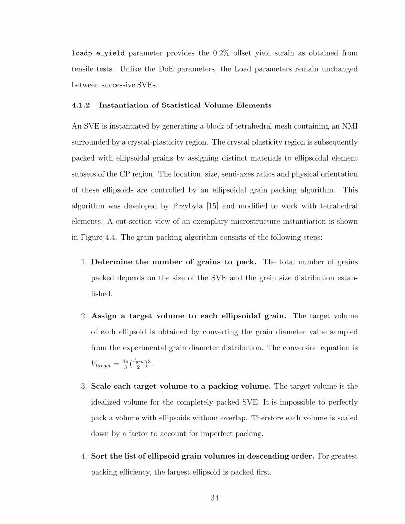
4.1.2 Instantiation of Statistical Volume Elements . . . . . . . . . 34
4.1.3 Mesh Quality Study . . . . . . . . . . . . . . . . . . . . . . . 38
4.2 Constitutive Model Parameter Fitting . . . . . . . . . . . . . . . . . 46
4.2.1 Calibration Experiments . . . . . . . . . . . . . . . . . . . . 46
4.2.2 Initial Parameter Calibration . . . . . . . . . . . . . . . . . . 49
4.2.3 Intermediate Parameter Calibration . . . . . . . . . . . . . . 51
4.2.4 Revised Parameter Calibration . . . . . . . . . . . . . . . . . 52
V RESULTS AND DISCUSSION . . . . . . . . . . . . . . . . . . . . . 55
5.1 FIP-Life Correlations . . . . . . . . . . . . . . . . . . . . . . . . . . 55
5.1.1 Effect of Inclusion Proximity to Surface . . . . . . . . . . . . 55
5.1.2 Identifying the Crack Incubation to Microcrack Growth Tran-sition . . . . . . . . . . . . . . . . . . . . . . . . . . . . . . . 64
VI CONCLUSIONS . . . . . . . . . . . . . . . . . . . . . . . . . . . . . . 73
VII RECOMMENDATIONS FOR FURTHER STUDY . . . . . . . . 75
7.1 Ranking of Microstructure Attributes by Fatigue Potency . . . . . . 75
7.1.1 NMI Morphology . . . . . . . . . . . . . . . . . . . . . . . . 75
7.1.2 NMI-matrix Interface . . . . . . . . . . . . . . . . . . . . . . 76
7.1.3 Alternative Crack Initiation Sites . . . . . . . . . . . . . . . 76
REFERENCES . . . . . . . . . . . . . . . . . . . . . . . . . . . . . . . . . . 78
v

LIST OF TABLES
2.1 Nominal chemical compositions of MP35N & 35N-LT given as wt %.From [2]. . . . . . . . . . . . . . . . . . . . . . . . . . . . . . . . . . . 5
3.1 Summary of main constitutive equations implemented by the UMAT 19
3.2 Volumes (in µm3) of the FIP AVs for a 4 µm cubic NMI. . . . . . . . 24
4.1 Independent (user defined) input parameters for microstructure gener-ation . . . . . . . . . . . . . . . . . . . . . . . . . . . . . . . . . . . . 29
4.2 Summary of size and run-time measures for the eight mesh density levels 41
4.3 Variables, parameters and coefficients used in constitutive relations . 45
4.4 Values of the constitutive parameters for the initial model calibration(UMAT v28) . . . . . . . . . . . . . . . . . . . . . . . . . . . . . . . 49
4.5 Results of DFT atomistic calculations for Ni-35Co-20Cr-10Mo alloycalculated at 0 Kelvin (ShunLi Shang, personal communication, 14August 2013). . . . . . . . . . . . . . . . . . . . . . . . . . . . . . . . 50
4.6 Values of the constitutive parameters for the intermediate model cali-bration (UMAT v110) . . . . . . . . . . . . . . . . . . . . . . . . . . 51
4.7 Values of the constitutive parameters for the revised model calibration(UMAT v110e) . . . . . . . . . . . . . . . . . . . . . . . . . . . . . . 53
5.1 Values of NMI geometry parameters at each level of the virtual DoE . 57
5.2 Relationships between beam-bending stress reported at the wire apex(Sa) and stress (SY Y ) and strain (εa) amplitudes applied to the SVE . 59
5.3 Fitting Parameters for GEV CDFs . . . . . . . . . . . . . . . . . . . 63
5.4 Fitting Parameters for Gumbel CDFs . . . . . . . . . . . . . . . . . . 64
vi
LIST OF FIGURES
2.1 Inclusions in MP35N fine wire. (a) Sharp cuboidal TiN inclusion, par-tially debonded from the matrix. (b) Globular Al2O3 (alumina) inclu-sion near the wire surface. Note differences in scale. From [19] . . . . 5
2.2 FIB cross-section micrograph illustrating the fine grain structure anddeformation twins. From [14]. . . . . . . . . . . . . . . . . . . . . . . 6
2.3 Grain size distributions of four wire cross-sections Af-1 through Af-4.From [7]. . . . . . . . . . . . . . . . . . . . . . . . . . . . . . . . . . . 7
2.4 EBSD accompanied by pole figures of low-Ti MP35N showing strong〈111〉 texture. From [14]. . . . . . . . . . . . . . . . . . . . . . . . . . 8
2.5 Configuration of wire fixed in a RBBF test system showing relevantparameters for fatigue loading. Taken from [2]. . . . . . . . . . . . . . 9
2.6 Illustration of the variation of normal stress across a wire cross-section 10
2.7 Schematic illustrating the dependence of Syy stress amplitude on thelocation of a material point within the wire. Point A experiences twicethe maximum stress of point B. . . . . . . . . . . . . . . . . . . . . . 10
2.8 CDFs of fatigue lives of MP35N and 35N-LT under RBBF at 827 MPastress amplitude. From [20] . . . . . . . . . . . . . . . . . . . . . . . 11
2.9 Effect of inclusion depth (filled circles) and size (open circles) on fatiguelife of MP35N wire at a stress amplitude of 620 MPa. From [20]. . . . 12
3.1 Schematic showing the positioning and naming conventions of selectedFS AVs with respect to a 50% debonded cuboidal inclusion. . . . . . 22
3.2 Measurement conventions for the FIP AVs with respect to a 50%debonded cuboidal NMI. . . . . . . . . . . . . . . . . . . . . . . . . . 23
4.1 Block diagram of information flow through the component parts of themodel, showing the software tools used for each step. . . . . . . . . . 27
4.2 Stress-fields around a cuboidal NMI with various interface debondingscenarios. (2) Top-only debond. (3) Upper-half debond (4) All butbottom debond. The NMI has been removed for clarity. . . . . . . . . 31
4.3 Volume fraction breakdown of texture components for four differentMP35N wire samples with four texture components each. From [7]. . 33
4.4 Cut-section view of an exemplary microstructure instantiation with1000 grains. Grains are delineated by color. The cuboidal TiN NMIparticle is shown in grey in the center. The width of the NMI is 4 µmand the SVE is 20 µm on each side. . . . . . . . . . . . . . . . . . . . 35
vii

4.5 2D illustration of ellipsoid grain placement showing coordinate systemsand naming conventions used. For clarity, only a few elements areshown, and the inclusion is excluded. . . . . . . . . . . . . . . . . . . 37
4.6 PDF of a representative microstructure instantiation with 1000 grainscomparing the achieved grain size distribution to the target distribution. 38
4.7 Targeted grain semi-axes ratios of a representative microstructure in-stantiation with 1000 grains. . . . . . . . . . . . . . . . . . . . . . . . 39
4.8 Cut-section view of SVE generated for mesh quality study showing 64cubic grains and central NMI. . . . . . . . . . . . . . . . . . . . . . . 40
4.9 Run-time (in seconds) for increasing number of elements along NMIedge. . . . . . . . . . . . . . . . . . . . . . . . . . . . . . . . . . . . . 42
4.10 Volume-averaged Full-Face FS response for increasing number of ele-ments along NMI edge. . . . . . . . . . . . . . . . . . . . . . . . . . . 43
4.11 Volume-averaged Mid-Face FS response for increasing number of ele-ments along NMI edge. . . . . . . . . . . . . . . . . . . . . . . . . . . 44
4.12 Strain-rate jump test on low-Ti MP35N as-drawn wire with strain ratealternating every 0.5% increment of strain. From [14]. . . . . . . . . . 47
4.13 Strain Ratcheting Experiments showing the accumulation of strain over300 cycles for Smax
1 = 1400 MPa and Smax2 = 1500 MPa. . . . . . . . 48
4.14 Plot of log(N) vs peak strain (mm/mm) for the LCF1 experiment.The rate of strain accumulation stabilizes after 10 cycles. . . . . . . . 48
4.15 Comparisons of the initial and intermediate parameter calibrations tothe rate jump uniaxial tension test. Experimental data from [14]. . . 52
4.16 Comparisons of the initial and intermediate parameter calibrations tothe LCF1 strain ratcheting experiment. . . . . . . . . . . . . . . . . . 53
4.17 Sensitivity of the effective elastic modulus to SVE texture. . . . . . . 54
5.1 Subset of an SVE showing definitions of TiN particle geometry as re-lated to the wire surface. . . . . . . . . . . . . . . . . . . . . . . . . . 56
5.2 Loading profile applied to each SVE to simulate RBBF. Points A andB are the step endpoints used in the FS FIP calculations. . . . . . . . 57
5.3 Selection of stress amplitude for an SVE. Stress amplitude SY Y de-creases linearly with NMI depth xc due to the stress gradient generatedin bending. Note that the x axis for depth is opposite the global X axis. 60
5.4 Extreme-value FS parameter values for four distinct NMI depths andcorresponding stress amplitudes . . . . . . . . . . . . . . . . . . . . . 61
viii
5.5 Life correlations of the model fit to experimental data. The modifiedT-M fit is performed at the 0.75 µm level resulting in a correlationcoefficient α of 1.129× 10⁻⁵ µm-cycles. . . . . . . . . . . . . . . . . . 62
5.6 CDFs of the Fatigue-life correlations with corresponding GEV distri-butions. . . . . . . . . . . . . . . . . . . . . . . . . . . . . . . . . . . 63
5.7 CDFs of the fatigue-life correlations with fitted Gumbel distributions. 64
5.8 Prasad et al. S-N data for as-drawn low-Ti MP35N wire [14]. . . . . . 66
5.9 Comparison of Extreme-Value FS parameter responses using weightingcoefficients k∗ = 1 and k∗ = 0.2. . . . . . . . . . . . . . . . . . . . . . 68
5.10 Fatigue-life correlation to Prasad et al. RBBF data at 620 MPa withT-M correlation coefficient α = 4.995× 10⁻⁷ µm-cycles. . . . . . . . . 69
5.11 Close-in view of the point of divergence between the T-M correlationto the RBBF data at 680 MPa and 1× 10⁵ cycles. . . . . . . . . . . . 70
5.12 Weighted variability (ΩFS) in EV FS response parameters at the fivestress amplitudes modeled with 10 microstructure instantiations each. 72
ix
SUMMARY
This work presents a model to assess the microstructure-sensitive high-cycle
fatigue (HCF) performance of thin MP35N alloy wires used as conductors in cardiac
leads. The major components of this model consist of a microstructure generator
that creates a mesh of a statistically representative microstructure, a finite element
analysis using a crystal plasticity constitutive model to determine the local response
behavior of the microstructure, and a postscript employing fatigue indicating param-
eters (FIPs) to assess the fatigue crack incubation potency at fatigue hotspots.
The crystal structure of the MP35N alloy, which contains major elements (wt %)
35Ni-35Co-20Cr-10Mo, is modeled as single-phase, face-centered cubic (fcc) material,
and the calibration of the constitutive behavior is based on monotonic tensile and
cyclic ratcheting stress-strain response data generated on the wire. A non-random
texture generation scheme is introduced to approximate the strong fiber texture de-
veloped by wire drawing. Non-metallic inclusions (NMIs) have been shown to be
detrimental in fatigue of MP35N wires by serving as fatigue crack nucleation sites.
The model developed here considers the detrimental effects of NMIs using a stochas-
tic framework. By evaluating multiple statistical volume elements (SVEs), the inher-
ent statistical variability of inclusion-grain and grain-grain interactions at the NMI-
matrix interface can be assessed. The fatigue crack incubation potency for selected
microstructure attributes, boundary and interface conditions, and loading profiles is
determined by computing the Fatemi-Socie (FS) multi-axial FIP over an appropriate
volume of scale.
The extreme-value FS distributions were successfully correlated to rotating beam
bending fatigue (RBBF) life data collected for MP35N fine wire. The correlation
x

indicates that the fatigue potency in RBBF is strongly influenced by the NMI prox-
imity to the wire surface with the most severe case occurring when the NMI intersects
the surface. A significant drop in fatigue potency is observed when the NMI is fully
embedded in the wire. Fatigue-life correlations to a second set of RBBF data were
performed in order to identify a transition life value between crack incubation and
microcrack growth fatigue mechanisms. The transition life was identified as 1 × 10⁵
cycles. The model has applications in numerous additional aspects of microstructure-
sensitive HCF which can be explored in a future work.
xi

CHAPTER I
INTRODUCTION
1.1 Motivation
A robust understanding of component fatigue behavior is critical for the medical
device industry especially for permanently implantable, life sustaining applications
where minimizing invasive procedures and treatments is highly desirable. In the case
of cardiac pacing leads, the in-situ loading conditions are variable and difficult to
quantify. Heart contractions create a low-amplitude, high-frequency load, and torso
and arm movements add higher amplitude, but low frequency loading. In the high
cycle fatigue regime, the fatigue life of fine wires is dominated by crack incubation.
Once formed, a fatigue crack grows quickly to reach the instability point due to the
geometric constraints of the wire, after which ductile (fast) fracture occurs. Fatigue
crack nucleation in fine wires is a stochastic process controlled by defects within the
microstructure. These defects occur in the drawn wire as surface scratches or non-
metallic inclusions (NMIs). Understanding the role these defects play in fatigue life
variability is critical to the design of fatigue resistant lead wires.
Past studies [20] have employed statistical Monte Carlo initiation life models to
predict such variability. However, these models are constrained by a limited capability
to represent the microstructure of the lead wires. Through the use of a crystal plas-
ticity finite element model (CPFEM) governed by a set of constitutive laws, many
different microstructural attributes can be modeled and quickly assessed for their
impact on fatigue. Analysis of process-structure-properties relationships using com-
putational tools is a key aspect of the Materials Genome Initiative (MGI) [12]. MGI
1

calls on governmental agencies, academic institutions and industrial partners to coop-
erate in accelerating the pace of materials development. The goal is to reduce by half
the typical material design lifecycle. The MGI infrastructure consists of three parts:
experimental tools, computational tools and data science tools. Once developed, these
tools can be adapted rapidly to collect and analyze material performance for different
materials, applications and processing routes. The current project contributes to the
computational tools aspect of materials development by creating software tools to
predict the high-cycle fatigue (HCF) performance of the MP35N alloy in the fine wire
configuration. Knowledge of the salient microstructure attributes also contributes to
the fundamental materials science understanding of this alloy.
1.2 Research Objective
The work presented in this thesis aims to link microstructure attributes of MP35N
fine wire with its HCF performance under application-relevant loading conditions
through the application of structure-property relations. At the present time, no
known CPFEM models have been developed for MP35N fine wire or for MP35N in
the bulk form. Although Schaffer [19] developed a numerical model for fine wire
MP35N incorporating the influence of a number of microstructural inputs via Monte
Carlo methods, his model does not account for polycrystalline plasticity which is
known to play a significant role in HCF. The objective of this research is to develop a
computational CPFEM model for MP35N fine wire capable of elucidating differences
in fatigue performance due to variability of microstructure attributes. This includes:
1. Formulation of constitutive relations that capture the rate sensitivity and kine-
matic hardening behavior of MP35N fine wire
2. Calibration of these constitutive relations to experimental data
3. Development of a microstructure generation and meshing protocol to recreate
2

salient MP35N microstructure attributes in a stochastic, finite-element frame-
work
4. Selection of appropriate response parameters to assess fatigue performance
5. Characterization of the extreme-value distributions of the selected response pa-
rameters
6. Validation of the newly-developed CPFEM model against experimental data
1.3 Thesis Layout
Chapter 2 provides background on the MP35N alloy system and the microstructure of
MP35N fine wires and reviews previous fatigue models and fatigue testing techniques.
Chapter 3 describes the modeling methodology employed in this research, including
the generation of virtual microstructures, constitutive model framework, selection of
fatigue indicating parameters and life correlation methods. Chapter 4 details the
computational implementation of the model into software codes and considers the
calibration of the constitutive model behavior using selected experiments. Chapter 5
presents the results of two studies using the newly developed model: (1) the effect of
NMI-surface proximity and (2) the identification of crack incubation to microcrack
growth transition life value. The implications of each study are also discussed. Chap-
ter 6 summarizes the main conclusions from the research. Finally, Chapter 7 proposes
some recommendations for further study to extend the development and applications
of the model in relation to the current effort.
3
CHAPTER II
BACKGROUND
2.1 MP35N Material Specifications
MP35N (ASTM F562) is a quaternary, low temperature superalloy. It has a nominal
composition of 35% nickel, 35% cobalt, 20% chromium and 10% molybdenum. The
full composition by weight percent as specified by ASTM [2] is given in Table 2.1.
The high amount of nickel produces a metastable fcc crystal structure. MP35N in the
bulk form was first developed by SPS technologies for use in NASA cryogenic fastener
applications. The fine wire form of MP35N has found use in surgical implants due
its excellent corrosion resistance and biocompatibility [13] as well as its high strength
and fatigue resistance. Applications include catheters, stylets and pacing leads.
Production of wires is accomplished by drawing a rod through successively smaller
dies with intermediate annealing steps. The drawing process produces significant
anisotropy in the material with strong texture components in the 001, 111 and
113 [7,14,23]. Drawing also contributes to a fine grain structure. Grain size for fine
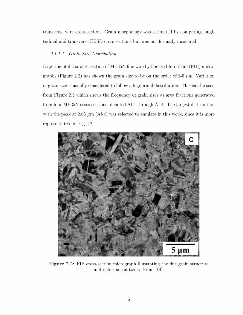
wire is typically 1-5 µm, compared with 35 µm or greater for the bulk material. Figure
2.2 is a FIB micrograph of a transverse section of the wire, revealing the fine grain
structure. In the bulk material, HCP platelets form through the Suzuki mechanism
[1, 5]. The HCP phase has not been observed in fine wire specimens [14, 23] or bulk
specimens under room-temperature deformation [17], leading to its characterization
as a single-phase material. Plastic deformation is accommodated through both slip
and intra-granular twinning [23]. Twins are found to be between 1-10 nm in thickness.
Once formed, deformation twins also act as a hardening mechanism, impeding the
motion of dislocations.
4
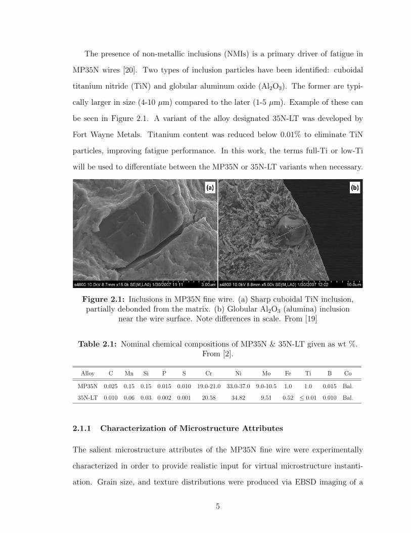
The presence of non-metallic inclusions (NMIs) is a primary driver of fatigue in
MP35N wires [20]. Two types of inclusion particles have been identified: cuboidal
titanium nitride (TiN) and globular aluminum oxide (Al2O3). The former are typi-
cally larger in size (4-10 µm) compared to the later (1-5 µm). Example of these can
be seen in Figure 2.1. A variant of the alloy designated 35N-LT was developed by
Fort Wayne Metals. Titanium content was reduced below 0.01% to eliminate TiN
particles, improving fatigue performance. In this work, the terms full-Ti or low-Ti
will be used to differentiate between the MP35N or 35N-LT variants when necessary.
Figure 2.1: Inclusions in MP35N fine wire. (a) Sharp cuboidal TiN inclusion,partially debonded from the matrix. (b) Globular Al2O3 (alumina) inclusion
near the wire surface. Note differences in scale. From [19]
Table 2.1: Nominal chemical compositions of MP35N & 35N-LT given as wt %.From [2].
Alloy C Mn Si P S Cr Ni Mo Fe Ti B Co
MP35N 0.025 0.15 0.15 0.015 0.010 19.0-21.0 33.0-37.0 9.0-10.5 1.0 1.0 0.015 Bal.
35N-LT 0.010 0.06 0.03 0.002 0.001 20.58 34.82 9.51 0.52 ≤ 0.01 0.010 Bal.
2.1.1 Characterization of Microstructure Attributes
The salient microstructure attributes of the MP35N fine wire were experimentally
characterized in order to provide realistic input for virtual microstructure instanti-
ation. Grain size, and texture distributions were produced via EBSD imaging of a
5
transverse wire cross-section. Grain morphology was estimated by comparing longi-
tudinal and transverse EBSD cross-sections but was not formally measured.
2.1.1.1 Grain Size Distribution
Experimental characterization of MP35N fine wire by Focused Ion Beam (FIB) micro-
graphs (Figure 2.2) has shown the grain size to be on the order of 1-5 µm. Variation
in grain size is usually considered to follow a lognormal distribution. This can be seen
from Figure 2.3 which shows the frequency of grain sizes as area fractions generated
from four MP35N cross-sections, denoted Af-1 through Af-4. The largest distribution
with the peak at 2.05 µm (Af-4) was selected to emulate in this work, since it is more
representative of Fig 2.2.
Figure 2.2: FIB cross-section micrograph illustrating the fine grain structureand deformation twins. From [14].
6

Figure 2.3: Grain size distributions of four wire cross-sections Af-1 throughAf-4. From [7].
2.1.1.2 Texture
MP35N in its cold-drawn condition exhibits a strong fiber texture produced as a result
of the wire drawing. The texture is shown in Figure 2.4. The texture map on the left
and pole figures on the right illustrate the concentrations around the 〈111〉 and 〈100〉
orientations.
7

Figure 2.4: EBSD accompanied by pole figures of low-Ti MP35N showingstrong 〈111〉 texture. From [14].
2.2 Rotating Beam Bending Fatigue
One type of fatigue experiment commonly conducted for fine wires is known as Ro-
tating Beam Bending Fatigue (RBBF). RBBF is an ASTM standardized test method
(E2948-14). A schematic of the wire configuration in the test system is shown in
Figure 2.5.
A length of wire is bent into a 180 degree arc and fixed at both ends by a rotary
chuck and bushing. Applying a rotational moment to the chuck results in a fully
reversed (R = −1) bending load as the wire rotates about its neutral axis. The
stresses and strains generated by RBBF can be determined from beam bending theory,
assuming purely elastic deformation and a homogeneous, isotropic material response.
The bending stress amplitude scales with the local wire curvature which is highest at
the wire apex, and approaches zero at either end. The magnitude of bending strain
at the apex is related to the minimum bend radius ρmin by the relation
8

Figure 2.5: Configuration of wire fixed in a RBBF test system showingrelevant parameters for fatigue loading. Taken from [2].
εa =d/2
ρmin(2.1)
where d is the wire diameter. The minimum bend radius is controlled by the center
distance C according to
ρmin = 0.417C (2.2)
and
C = 1.198E d
Sa(2.3)
where E is the elastic modulus of the wire, and Sa is the fully-reversed stress ampli-
tude. The wire length L and loop height h are related to C by constant factors. The
bending produces a non-uniform stress profile across the wire cross-section, driven by
the bending moment about the neutral axis as shown in Figure 2.6.
The outer fiber of the wire is loaded in tension while the inner fiber undergoes
compression. The maximum tensile and compressive stresses have equal magnitude
but opposite sign. As the wire rotates about its neutral axis each material point in
9
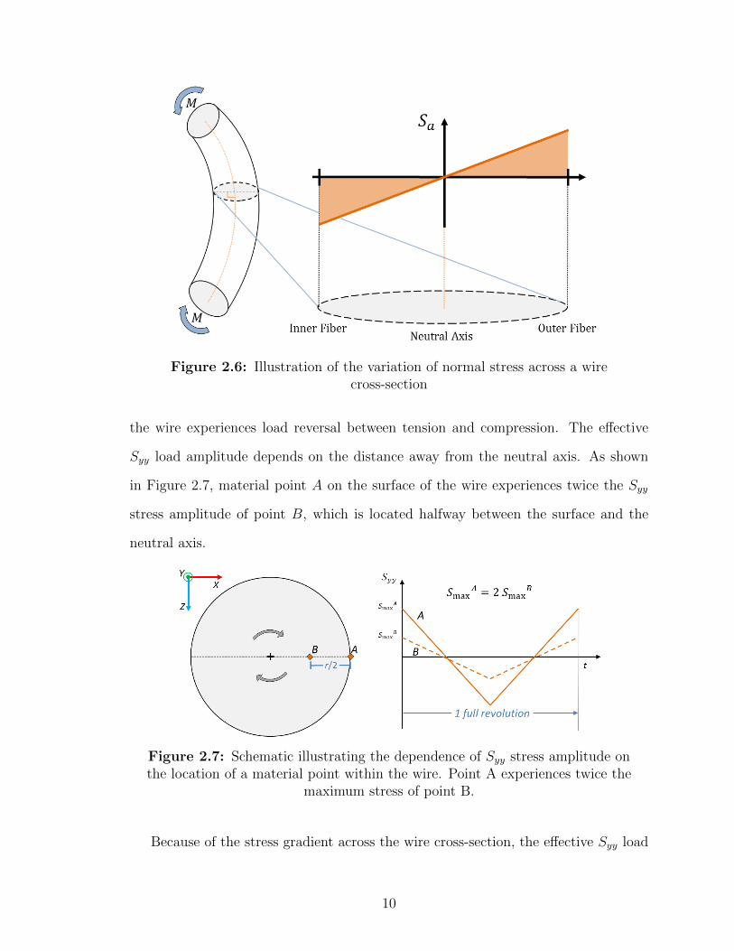
Figure 2.6: Illustration of the variation of normal stress across a wirecross-section
the wire experiences load reversal between tension and compression. The effective
Syy load amplitude depends on the distance away from the neutral axis. As shown
in Figure 2.7, material point A on the surface of the wire experiences twice the Syy
stress amplitude of point B, which is located halfway between the surface and the
neutral axis.
Figure 2.7: Schematic illustrating the dependence of Syy stress amplitude onthe location of a material point within the wire. Point A experiences twice the
maximum stress of point B.
Because of the stress gradient across the wire cross-section, the effective Syy load
10

amplitude at the site of crack initiation depends strongly on the distance of the site
from the neutral axis. In the absence of complicating microstructural factors, the
far-field loading conditions favor crack formation at the free surface. However, it is
conceivable for a fatigue crack to initiate away from the surface if microstructural
attributes located there combine to provide a significant driving force.
2.3 Schaffer Fatigue Results
An in-depth study of RBBF fatigue of the MP35N alloy system was conducted by
Schaffer [19] in both the LCF and HCF regimes. Both the low and full Ti alloy variants
were investigated. It was shown that the low-Ti alloy variant, 35N-LT performed
better in RBBF than its counterpart, as seen in the cumulative distribution function
(CDF) of Figure 2.8. Moreover, the 35N-LT data revealed a bimodal life distribution,
with one group of failures occurring in the range between 2.2×10⁵ and 2×10⁶ cycles,
while a separate group of failures occurred in a higher range at greater than 1× 10⁷
cycles.
Figure 2.8: CDFs of fatigue lives of MP35N and 35N-LT under RBBF at 827MPa stress amplitude. From [20]
11

The separation between the two groups was attributed to differences in the crack
initiation site: in the lower range group cracks predominantly formed by small (1-5
µm) alumina inclusions at or very near the surface, while in the higher cycle group
cracks initiated at subsurface particles greater than 0.5 µm below the surface. The
dependence of fatigue life on inclusion particle depth from the surface is also present
in the full-Ti version of the alloy albeit at lower stress amplitudes. This trend is
illustrated in Figure 2.9. Here filled circles denote the inclusion depth from the wire
surface and open circles represent the size of each inclusion, such that each fatigue
experiment performed is displayed by two points – one filled and one open – on the
plot.
Figure 2.9: Effect of inclusion depth (filled circles) and size (open circles) onfatigue life of MP35N wire at a stress amplitude of 620 MPa. From [20].
2.4 Microstructure-sensitive Fatigue Modeling
Microstructure-sensitive fatigue models are attempts to represent scatter in fatigue life
by explicitly considering the effects of microstructure. The microstructure attributes
12

considered may include grain size and texture, phases, precipitates, non-metallic in-
clusions, voids or other pre-existing flaws at the scale of the microstructure.
The major components of a microstructure-sensitive fatigue model involve:
1. A representation of one or more microstructural attributes which vary in con-
formance to some prescribed distributions
2. A method for applying representative fatigue loading and tracking the evolution
of local stresses and strains
3. A metric to evaluate fatigue damage potency. This involves combining key re-
sponse parameters in a manner that provide an indication of the fatigue damage
potency of the applied loading in light of the microstructure attributes repre-
sented. Response parameters include stress-based, strain-based, energy-based
or critical-plane based response parameters.
Historically, empirical methods of have been used to provide an estimation of fa-
tigue life. The most well-known of these approaches are the Basquin equation for
HCF and the Coffin-Manson equation for LCF [24]. The combination of these two
equations via Hookes law provides a fatigue equation which spans high and low cycle
fatigue. Various modifications have been proposed to adapt this model to non-zero
mean stress, notch effects, etc. These empirical methods rely on extensive fatigue
experiments to fit their coefficients and convey no information about the microstruc-
ture. Microstructure-sensitive fatigue models implemented with modern computa-
tional tools can better represent known physical phenomena that lead to fatigue in-
cluding slip localization and plastic strain heterogeneity due to geometrical features
(notches etc) and grain-grain and grain-inclusion interactions.
Some of the specific applications of microstructure-sensitive fatigue models are as
follows:
13

1. Link experimentally observed scatter in fatigue life data to known damage mech-
anisms
2. Provide an estimate of minimum fatigue life for a given alloy, processing, and
cyclic loading history
3. Establish rankings of microstructure attributes most detrimental to life.
These applications have been considered in recent work. Musinski [11] imple-
mented a crystal plasticity finite element model to examine microstructurally small
fatigue crack growth in both smooth and notched Ni-base superalloy specimens in-
corporating the effect of debonded inclusion particles and grain boundary effects.
Przybyla [16] used extreme-value marked correlation functions to identify and rank
the influence of coupled microstructure attributes (grain orientation, misorientation
and size) on fatigue damage in a Ni-base superalloy and two Ti alloys. Salajeghah [18]
used weighted probability functions to investigate the surface to bulk transition in
HCF crack initiations in both IN100 and C61 martensitic gear steel.
2.5 Fatigue Life Considerations
Life to failure of a metallic component is traditionally divided into initiation life and
propagation life according to the equation
Nf = Ninc +Np (2.4)
Here, Ninc is the number of cycles required to incubate a crack, Np is the number of
cycles for the crack to propagate to failure. Propagation life can be further subdivided
three crack growth regimes as
Np = Nmsc +Npsc +Nlc (2.5)
14

where Nmsc is the number of cycles from formation to a microstructurally small
crack, Npsc is the number of cycles to grow to a physically small crack, and Nlc
defines the long crack growth regime, which typically begins when the crack reaches
the visual inspection limit through the onset of fast fracture. The boundaries of the
crack growth regimes are not well defined. For the purposes of this model, we neglect
the contribution of propagation life to the total life in MP35N wire fatigue based on
the following reasoning:
1. Once incubated, cracks propagate to reach the instability point in relatively few
cycles due to the small cross-sections of the fine wires.
2. The change in Np with decreasing stress amplitude is minimal.
3. Under HCF and VHCF conditions the total cycles to failure is large, and the
great majority of these contribute to crack incubation.
A simple example can illustrate this reasoning. Suppose the propagation life for
any stress amplitude is the same, Np = 10, 000 cycles. Now consider two HCF RBBF
specimens, one failing at Nf = 100, 000 cycles, and another at Nf = 1, 000, 000 cycles.
For the first specimen, 10% of all cycles are propagation, and for the second specimen
only 1% of the total life is propagation. Based on this consideration, it is judged that
the contribution to the fatigue life from crack propagation in the HCF regime will be
less than 10% and can be neglected for the purposes of this model.
15

CHAPTER III
MODELING METHODOLOGY
3.1 Microstructure Generation and SVEs
In order to model the stochastic nature of metallic microstructures in a computation-
ally feasible way, it is useful to employ Statistical Volume Elements (SVEs). These
idealized volumes are constructed such that each identically-sized volume is a sample
of the underlying distributions of the microstructure attributes. Each SVE contains a
unique, random arrangement of grains and crystallographic textures which are sam-
pled from experimentally characterized grain size and texture distributions.
The size of the volume must meet certain criteria to qualify as an SVE. The
volume must be of the same length scale as the response parameters of interest, i.e.
grain-scale plasticity. Additionally, the volume must be small enough such that the
distribution of the local response parameters of interest within each SVE comprises
a subset of all possible values. The SVE volume should be large enough relative to
the grain size that the average stress-strain responses of multiple SVEs converges to
the macroscopic stress-strain response determined by experiment.
The use of SVEs for numerical fatigue modeling offers advantages in computa-
tional efficiency. A limited number of SVEs (< 100) at each loading condition can
adequately characterize the distribution of the desired response parameter. Variation
of microstructure attributes between successive SVEs results in differences in the local
stress-strain response. These differences can be quantified using Fatigue Indicating
Parameters (FIPs) which serve as a proxy measure for fatigue crack formation.
16
3.2 Constitutive Model
The constitutive model for fine wire MP35N is adapted from a previous model by
Shenoy [21] for Inconel 100, a Ni-based superalloy. The constitutive model describes
the elastic and inelastic deformation through a set of equations derived from crystal
plasticity and continuum mechanics. The shear strain rate γ depends on shear stress
τ , and the evolution of two internal state variables (ISVs) – dislocation density ρ and
backstress χ. In the fine wire configuration, MP35N consists of a single-phase FCC
structure with intra-granular deformation twins. Slip is permitted only on the 12
octahedral systems 〈110〉 111. Deformation twins are not explicitly modeled, but
are accounted for phenomenologically through two input parameters: twin volume
fraction ftw and twin spacing, t. Homogenization over deformation twins is necessary
due to the limited spatial resolution of finite element modeling. The model seeks to
predict damage processes at the scale of microns, while deformation twins have been
shown by TEM imaging to have thicknesses of 1-10 nanometers [14,23].
3.2.1 Inelastic Constitutive Equations
The inelastic shear strain rate on slip system α is given by a single-term flow rule
γ(α) = γo
⟨|τ (α) − χ(α)|−κ(α)
D(α)
⟩nsgn(τ (α) − χ(α)) (3.1)
where γo is a shear strain rate constant, D is the drag stress, n is the flow exponent
and κ is the threshold hardening parameter. D and n are fitting parameters that
describe the resistance to plastic flow and the strain rate sensitivity, respectively.
The second term used by Shenoy to account for thermally activated flow is removed
for this isothermal model. Inelastic shear strain is zero until an isotropic threshold
stress κ is attained. The threshold hardening equation depends on dislocation density
ρ through a Taylor relation
κ(α) = κ(α)o + αtµb
√ρ(α) (3.2)
17
where b is the burgers vector of MP35N, µ is the (resolved) shear modulus, αt is a
constant and κo is the initial critical resolved shear stress (CRSS) given by
κ(α)o = [(τ (α)
o )nk + cgr(dgr)−0.5 + cgr(ftw)]
1nk (3.3)
which depends on the lattice resistance, τo, the nominal grain size, dgr, and the twin
volume fraction ftw as well as constants cgr and nk. Dislocation density ρ evolves by
the equation
ρ(α) =12∑β=1
h(αβ)
(k1
bΛ(β)− k2ρ
(β)
)|γ(β)| (3.4)
Here k1 and k2 are constants, h(αβ) is the hardening coefficient matrix, and Λ is the
mean free path (MFP) for dislocation motion. The dislocation density affects both
isotropic and kinematic hardening, as seen in Eqs. 3.2 and 3.7. At high dislocation
densities typical of strongly cold-worked components, competition between dislocation
formation and annihilation results in saturation of ρ due to the dynamic equilibrium
between the first and second terms of Eq. 3.4. The hardening coefficient matrix takes
the form
h(αβ) = hoδ(αβ) (3.5)
where ho is a constant and δ is the Kronecker delta. Here α = β represents self-
hardening slip systems and α 6= β represents latent slip or cross-hardening. Due to the
low stacking-fault energy (SFE) of MP35N, cross-slip is assumed to be negligible. The
MFP Λ is a measure of the obstacle-free movement distance available to a dislocation
on a given slip system. In MP35N, it is described by the harmonic mean of three
distances: the grain size dgr, twin spacing t and the spacing of immobile dislocations
which scales inversely with the square root of dislocation density.
1
Λ(β)=
1
dgr+
1
t+ k3
√ρ(β) (3.6)
The backstress evolves according to
χ(α) = Cχ[ηµb√ρ(α)sgn(τ (α) − χ(α))− χ(α)]|γ(α)| (3.7)
18

where Cχ is a fitting parameter and η depends on dgr, t and Λ by the relation
η = ηoΛ(α)
(1
dgr+
1
t
)(3.8)
The backstress equation contains two terms: an accumulation term that depends on
the dislocation density on the current slip system, and a dynamaic recovery term
dependent on the current value of χ representing the influence of dislocation anni-
hilation. The backstress ISV captures the Bauschinger effect and plastic ratcheting
that occurs under cyclic loading as a result of non-uniform dislocation pile-up at
grain and twin boundaries. The constitutive equations implemented by the model
are summarized in Table 3.1.
Table 3.1: Summary of main constitutive equations implemented by the UMAT
Flow Rule γ(α) = γo
⟨|τ (α)−χ(α)|−κ(α)
D(α)
⟩nsgn(τ (α) − χ(α))
Threshold Hardening κ(α) = κ(α)o + αtµb
√ρ(α)
Initial CRSS κ(α)o = [(τ
(α)o )nk + cgr(dgr)
−0.5 + cgr(ftw)]1nk
Backstress Evolution χ(α) = Cχ[ηµb√ρ(α)sgn(τ (α) − χ(α))− χ(α)]|γ(α)|
Eta η = ηoΛ(α)
(1dgr
+ 1t
)Dislocation Density Evolution ρ(α) =
∑12β=1 h
(αβ)
(k1
bΛ(β) − k2ρ(β)
)|γ(β)|
Hardening Coefficients h(αβ) = hoδ(αβ)
Mean Free Path 1Λ(β) = 1
dgr+ 1
t+ k3
√ρ(β)
3.3 Fatigue Indicator Parameters
Fatigue Indicator Parameters (FIPs) provide a way to determine the location and
relative potency of fatigue hot-spots within a component after the application of
19

fatigue loading. FIPs are physically-based metrics that combine tensor quantities
such as stresses or plastic strains occurring over a representative load cycle into a
single scalar value which can be used to judge the relative fatigue potency. Numerous
FIPs have been proposed and utilized for different materials and crack formation
mechanisms.
3.3.1 Fatemi-Socie Parameter
The Fatemi-Socie (FS) parameter [6] was selected for use with the model for its ability
to predict fatigue response in materials where crack formation is driven by localized
cyclic shear strain. The parameter is based on the observation that cyclic fatigue
cracks tend to form on planes aligned with the direction of maximum shear strain
amplitude, but that magnitude of shear strain amplitude alone does not explain the
lower rates of cracking in torsional fatigue compared to uniaxial. To account for this,
the maximum plastic shear strain amplitude over a cycle is modified by the normal
stress to the plane of maximum plastic shear strain. The FS parameter is given by
PFS =∆γpmax
2
[1 + k∗
σmaxn
σY
](3.9)
where ∆γpmax is the maximum range of plastic shear strain on the critical plane over
a cycle and σmaxn is the maximum stress normal to the critical plane. The maximum
normal stress is normalized by the yield stress σY and weighted by the coefficient
k∗. The weighting coefficient can be estimated by correlating uniaxial to torsional
fatigue data. Lacking torsional data for MP35N fine wire, k∗ has been arbitrarily
set to 1, which is within the range of values found in fatigue literature [3, 11]. The
FS parameter as formulated in Eq. 3.9 is termed a critical plane type FIP since
it accounts for preferential crack nucleation on cyclic shear planes. Musinski [9]
considered two distinct critical plane types, crystallographic or non-crystallographic.
The crystallographic formulation finds the critical plane by searching all available
slip systems, while the non-crystallographic formulation takes the plane of maximum
20
cyclic shear strain in 3D space. The non-crystallographic formulation is used in this
work to simplify computation. The choice of critical plane calculation methodology
is not expected to significantly impact the parameter scaling.
3.3.2 Selection of Averaging Volumes
The FS parameter must be evaluated over an appropriate volume in order to provide
a meaningful indication of fatigue crack formation potency. Two important consider-
ations for averaging volume (AV) selection are size and sampling location within the
SVE.
3.3.2.1 Size Considerations
Volume size is dictated by (a) the finite size of fatigue crack incubation, (b) regu-
larization to eliminate mesh-size dependency and (c) desired level of smoothing over
microstructural features such as grains. The term incubation is not well-defined in
literature, having no single agreed-upon criteria. For the purposes of this research,
a fatigue crack is considered incubated when the cracked area within the matrix
approaches 1 µm2. Therefore, the size of the volumes used will be of this same scale.
3.3.2.2 Sampling Location Considerations
Sampling location is associated with the locations of stress risers within the mi-
crostructure which provide the driving force for crack initiation. In many cases, the
locations of stress risers are unknown a-priori so the entire SVE must be interro-
gated to locate them. However, when a hard NMI is present within the SVE, stress
concentrations will occur along the inclusion-matrix interface, permitting a targeted
application of sampling locations there. Salajegheh [18] found that inclusions which
are half debonded from the matrix in an orientation perpendicular to the loading axis
will generate their maximum stresses along the debonding perimeter. Under HCF
conditions, stresses quickly approach their far-field values moving radially outward
21
away from the NMI surface, resulting in insufficient driving force to generate plas-
ticity more than a few microns from the NMI interface. Because of this, AVs are
sampled immediately adjacent to the NMI. Salajegheh showed that this sampling lo-
cation corresponded to the locations of largest FIP magnitude for the 50% debonded
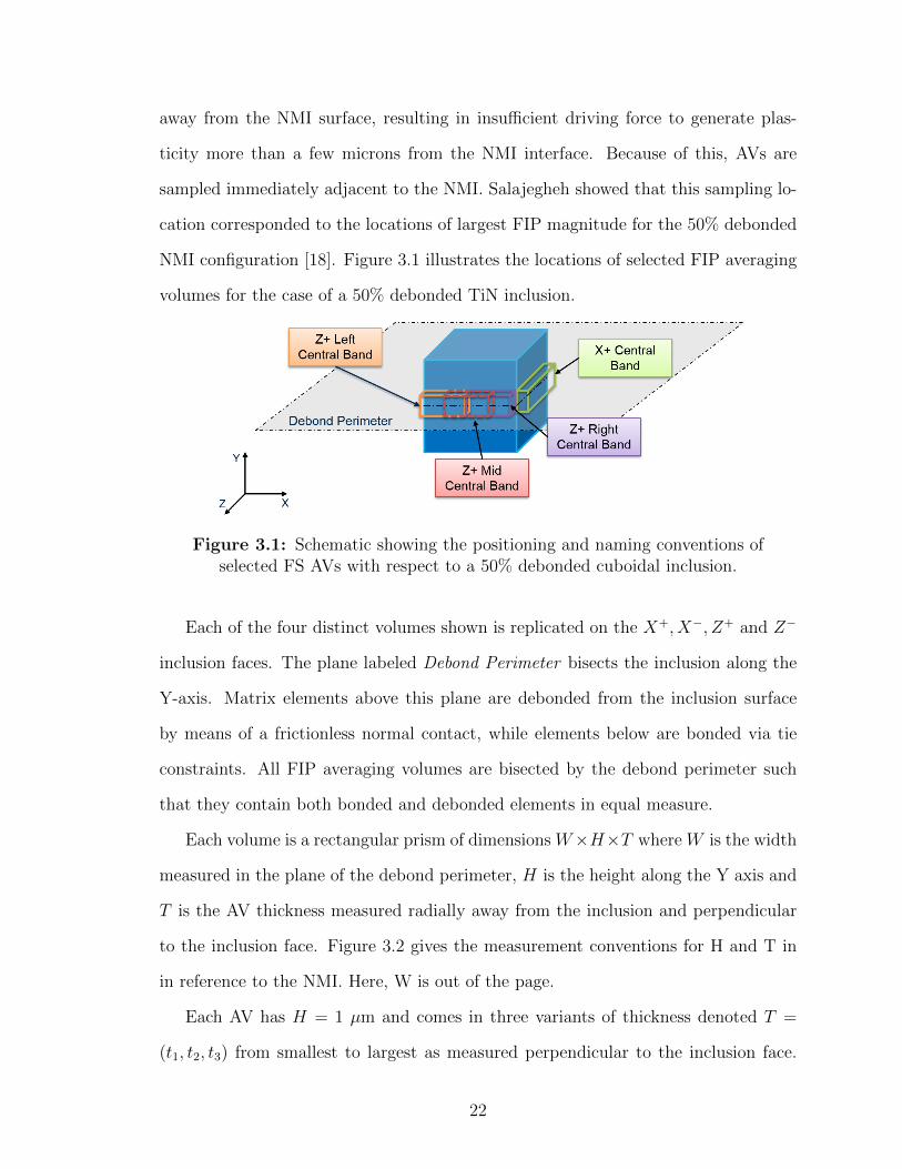
NMI configuration [18]. Figure 3.1 illustrates the locations of selected FIP averaging
volumes for the case of a 50% debonded TiN inclusion.
Figure 3.1: Schematic showing the positioning and naming conventions ofselected FS AVs with respect to a 50% debonded cuboidal inclusion.
Each of the four distinct volumes shown is replicated on the X+, X−, Z+ and Z−
inclusion faces. The plane labeled Debond Perimeter bisects the inclusion along the
Y-axis. Matrix elements above this plane are debonded from the inclusion surface
by means of a frictionless normal contact, while elements below are bonded via tie
constraints. All FIP averaging volumes are bisected by the debond perimeter such
that they contain both bonded and debonded elements in equal measure.
Each volume is a rectangular prism of dimensions W×H×T where W is the width
measured in the plane of the debond perimeter, H is the height along the Y axis and
T is the AV thickness measured radially away from the inclusion and perpendicular
to the inclusion face. Figure 3.2 gives the measurement conventions for H and T in
in reference to the NMI. Here, W is out of the page.
Each AV has H = 1 µm and comes in three variants of thickness denoted T =
(t1, t2, t3) from smallest to largest as measured perpendicular to the inclusion face.
22
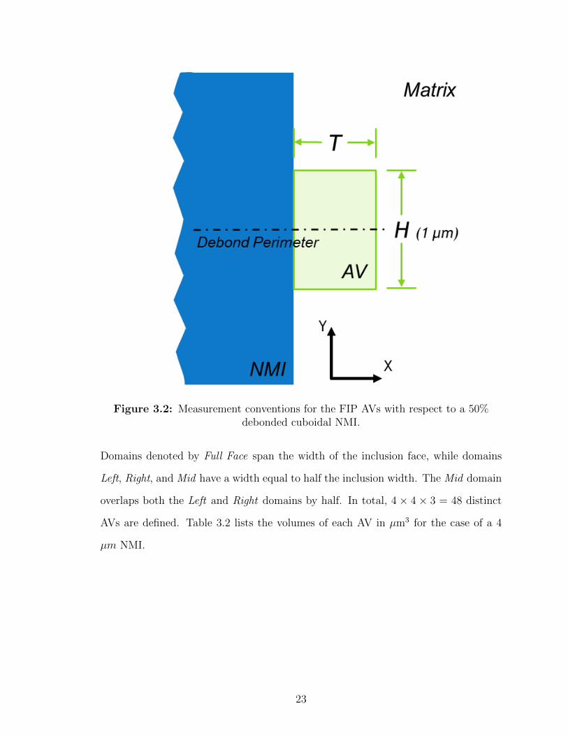
Figure 3.2: Measurement conventions for the FIP AVs with respect to a 50%debonded cuboidal NMI.
Domains denoted by Full Face span the width of the inclusion face, while domains
Left, Right, and Mid have a width equal to half the inclusion width. The Mid domain
overlaps both the Left and Right domains by half. In total, 4 × 4 × 3 = 48 distinct
AVs are defined. Table 3.2 lists the volumes of each AV in µm3 for the case of a 4
µm NMI.
23

Table 3.2: Volumes (in µm3) of the FIP AVs for a 4 µm cubic NMI.
AV Identifier t1(0.10 µm)
t2(0.25 µm)
t3(0.50 µm)
Full Face 0.4 1.0 2.0
Left Face 0.2 0.5 1.0
Mid Face 0.2 0.5 1.0
Right Face 0.2 0.5 1.0
3.4 Extreme Value Statistics
Statistics of extreme values (ie maxima and minima) are useful in the study of the
fatigue behavior of engineering components. Engineering components used in life-
critical applications must be designed to make the likelihood of fatigue failure ex-
tremely small. Prediction of reliability requires characterization of the behavior of
the tail end of the population which fails prior to its designed lifespan. Extreme value
statistics characterize this tail. Three classes of extreme-value distributions – Gumbel
(Type I), Frechet (Type II) and Weibull (Type III) – can be described by a single
distribution through the addition of a shape parameter. This combined distribution
is known as the Generalized Extreme Value (GEV) distribution. The cumulative
distribution function (CDF) for the GEV distribution is given by
FGEV(x;µ, σ, ξ) = e−[1+ξ(x−µσ
)]−1/ξ
(3.10)
where µ is the location parameter, σ is the scale parameter and ξ is the shape param-
eter. Parameters µ and σ are permitted to be any real number, but ξ is restricted to
the interval [-1,1]. The shape parameter significantly alters the behavior of the GEV
distribution depending on whether ξ > 0, ξ = 0 or ξ < 0. In the case of ξ = 0, Eq.
3.10 is undefined and must be replaced by the limit as ξ → 0 resulting in
FGumbel(x;µ, σ, 0) = e−e(−x−µ
σ )
(3.11)
24

also known as the Gumbel or Type I GEV distribution. In this work, the GEV distri-
bution (Eq. 3.10) is used to fit the distributions of the volume-averaged FS parameter
and the corresponding fatigue life correlations. The GEV fit is also compared to the
Gumbel distribution fit of Eq. 3.11 for the same data.
3.5 Correlation to Life
Once a sufficiently large sample of the extreme-value FS response values has been
constructed from multiple microstructure instantiations, the sample can then be cor-
related to a life distribution using a modified Tanaka-Mura (T-M) approach [25] [3].
The Tanaka-Mura equation considers that the number of cycles required to incubate
a crack along a slip band under HCF loading is related to the energy required to
form new surfaces which is inversely proportional to the square of the cyclic plastic
shear strain range ∆γp. By substituting the extreme-value FS parameter for ∆γp,
the following relation emerges [22]:
Ninc =α
dgr(PFS)−2 (3.12)
where Ninc is the number of cycles required to incubate a fatigue crack, dgr is a
scaling parameter associated with the microstructural size scale and α is a correlation
coefficient, determined by fitting the extreme-value FS distribution to an experimental
life distribution.
25

CHAPTER IV
COMPUTATIONAL IMPLEMENTATION
The CPFEM model developed in this work consists of three main components:
1. A microstructure generation tool that creates the stochastic arrangement of
grains within the defined volume;
2. A finite element solver coupling to a physically based constitutive model imple-
mented numerically though a UMAT that iteratively solves for the local stress
and strain states;
3. A postprocessing script to extract the local response variables, specifically the
volume-averaged Fatemi-Socie Parameter.
This chapter will deal with the implementation of these components within a
computational framework including all necessary data inputs and expected outputs.
Figure 4.1 provides a summary of the CPFEM model highlighting the flow of infor-
mation and the necessary software tools for implementation.
The finite element meshes are created with python scripting for ABAQUS, and
the grains are assigned via a Matlab [8] script. Each microstructure instantiation
undergoes a simulated fatigue loading history in the commercial finite element soft-
ware package ABAQUS [4]. ABAQUS calls to a custom-built crystal-plasticity User
MATerial subroutine (UMAT) implemented in Fortran, which computes the stress-
strain response over the entire mesh at each timestep. Prior to analysis, both the
microstructure generation tool and the UMAT are calibrated using a combination
of experimental data and values from literature. The continuum mechanics basis
for the UMAT is presented in Sec 3.2. After the simulated fatigue cycling has been
26

Figure 4.1: Block diagram of information flow through the component partsof the model, showing the software tools used for each step.
completed, a Matlab post-script computes the volume-averaged FS FIPs for each mi-
crostructure instantiation based on the local values of the stress and plastic strain
tensors.
Once the FIPs have been calculated, the extreme-value FS distribution is popu-
lated from the maximum FS value of each microstructure instantiation. The distri-
bution of extreme-value FIPs are then correlated to the distribution of fatigue life
values found by experiment though a modified Tanaka-Mura approach as described
in Sec 3.5. The fatigue life correlation provides a direct quantitative comparison of
the CPFEM model data to experimental fatigue data and can be used to predict
fatigue life curves. The following sections provide detailed explanations of the model
implementation in the code.
27

4.1 Microstructure Generation and Meshing
The microstructure is created using an ellipsoid packing algorithm developed by
Przybyla [15] and uses a meshing algorithm based on Musinski’s work [10]. The
target microstructure is a small volume of a MP35N fine-wire matrix surrounding a
cuboidal TiN inclusion particle. Since the goal of the model is to examine rare event
phenomenon associated with NMIs, the inclusion is input deterministically to each
instantiation with full control of inclusion size, position and interface. The loading,
interface and boundary conditions around the NMI can all be manipulated to examine
their effect on fatigue potency.
4.1.1 User Input Parameters
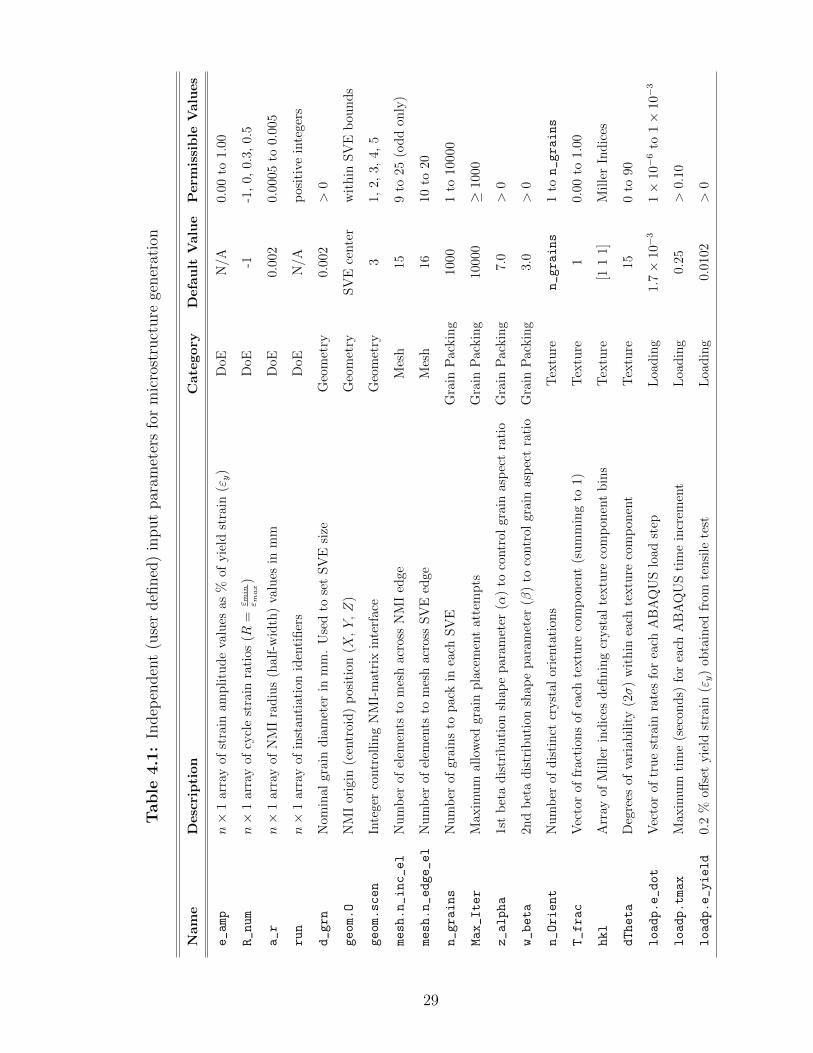
Table 4.1 summarizes the user input parameters for microstructure generation, along
with their default and permissible values. Each input parameter is the name of a
variable in the Matlab code which can be set by the user. The input parameters
are broken out into six categories: DoE, Geometry, Mesh, Grain Packing, Texture
and Loading. The following sections describe the functions of each of the user input
parameters by category.
28
Table
4.1
:In
dep
enden
t(u
ser
defi
ned
)in
put
par
amet
ers
for
mic
rost
ruct
ure
gener
atio
n
Nam
eD
esc
ripti
on
Cate
gory
Defa
ult
Valu
eP
erm
issi
ble
Valu
es
e_amp
n×
1ar
ray
ofst
rain
amp
litu
de
valu
esas
%of
yie
ldst
rain
(εy)
DoE
N/A
0.00
to1.
00
R_num
n×
1ar
ray
ofcy
cle
stra
inra
tios
(R=
ε min
ε max)
DoE
-1-1
,0,
0.3,
0.5
a_r
n×
1ar
ray
ofN
MI
rad
ius
(hal
f-w
idth
)va
lues
inm
mD
oE0.
002
0.00
05to
0.00
5
run
n×
1ar
ray
ofin
stan
tiat
ion
iden
tifi
ers
DoE
N/A
pos
itiv
ein
tege
rs
d_grn
Nom
inal
grai
nd
iam
eter
inm
m.
Use
dto
set
SV
Esi
zeG
eom
etry
0.00
2>
0
geom.O
NM
Ior
igin
(cen
troi
d)
pos
itio
n(X,Y,Z
)G
eom
etry
SV
Ece
nte
rw
ith
inS
VE
bou
nd
s
geom.scen
Inte
ger
contr
olli
ng
NM
I-m
atri
xin
terf
ace
Geo
met
ry3
1,2,
3,4,
5
mesh.n_inc_el
Nu
mb
erof
elem
ents
tom
esh
acro
ssN
MI
edge
Mes
h15
9to
25(o
dd
only
)
mesh.n_edge_el
Nu
mb
erof
elem
ents
tom
esh
acro
ssS
VE
edge
Mes
h16
10to
20
n_grains
Nu
mb
erof
grai
ns
top
ack
inea
chS
VE
Gra
inP
ackin
g10
001
to10
000
Max_Iter
Max
imu
mal
low
edgr
ain
pla
cem
ent
atte
mp
tsG
rain
Pac
kin
g10
000
≥10
00
z_alpha
1st
bet
ad
istr
ibu
tion
shap
ep
aram
eter
(α)
toco
ntr
olgr
ain
asp
ect
rati
oG
rain
Pac
kin
g7.
0>
0
w_beta
2nd
bet
ad
istr
ibu
tion
shap
epar
amet
er(β
)to
contr
olgr
ain
asp
ect
rati
oG
rain
Pac
kin
g3.
0>
0
n_Orient
Nu
mb
erof
dis
tin
ctcr
yst
alor
ienta
tion
sT
extu
ren_grains
1to
n_grains
T_frac
Vec
tor
offr
acti
ons
ofea
chte
xtu
reco
mp
onen
t(s
um
min
gto
1)T
extu
re1
0.00
to1.
00
hkl
Arr
ayof
Mil
ler
ind
ices
defi
nin
gcr
yst
alte
xtu
reco
mp
onen
tb
ins
Tex
ture
[11
1]M
ille
rIn
dic
es
dTheta
Deg
rees
ofva
riab
ilit
y(2σ
)w
ith
inea
chte
xtu
reco
mp
onen
tT
extu
re15
0to
90
loadp.e_dot
Vec
tor
oftr
ue
stra
inra
tes
for
each
AB
AQ
US
load
step
Loa
din
g1.
7×
10−
31×
10−
6to
1×
10−
3
loadp.tmax
Max
imu
mti
me
(sec
ond
s)fo
rea
chA
BA
QU
Sti
me
incr
emen
tL
oad
ing
0.25
>0.
10
loadp.e_yield
0.2
%off
set
yie
ldst
rain
(εy)
obta
ined
from
ten
sile
test
Loa
din
g0.
0102
>0
29

4.1.1.1 DoE Parameters
The four DoE parameters e_amp, R_num, a_r and run, are used to construct the SVEs
necessary to run an arbitrary sized virtual Design of Experiements (DoE). The DoE
has three factors associated with strain amplitude (e_amp), strain ratio (R_num) and
NMI half-width (a_r). Each factor may have an arbitrary number of levels taking on
any of the permissible values as set by the user. At least one SVE is created for every
combination of factor levels. The number of microstructure instantiations created at
each point in the DoE is determined by the run parameter. The run parameter is the
set of sequential positive integers which provides a unique run ID to each microstruc-
ture created. By way of example, the input e_amp = [0.30, 0.45, 0.60], R_num = [−1],
a_r = [0.002], run = [1, 2, 3, 4, 5] generates five microstructure instantiations at each
of three strain amplitudes with R = −1 and rNMI = 0.002 mm, resulting a total of
15 parameterized SVEs.
4.1.1.2 Geometry Parameters
The geometry parameters d_grn, geom.O and geom.scen control the nominal grain
size, NMI centroid position and NMI matrix-interface condition respectively. The
SVE edge length is ten times d_grn in order to avoid undue influence of a single grain
on the SVE mechanical response behavior. The NMI origin (centroid) is set by geom.O
which is a vector in SVE global coordinates (X, Y , Z). The geom.scen parameter
is an integer which selects from five preset NMI interface conditions. The five preset
interface conditions are (1) completely bonded, (2) Top-only bonded, (3) Upper-half
debond, (4) all but bottom debond and (5) solid mesh without NMI. Figure 4.2
illustrates scenarios 2-4 and the resulting stress fields. The red highlighting indicates
the mesh regions where tie constraints are applied to create a bonded interface.
30

Figure 4.2: Stress-fields around a cuboidal NMI with various interfacedebonding scenarios. (2) Top-only debond. (3) Upper-half debond (4) All but
bottom debond. The NMI has been removed for clarity.
4.1.1.3 Mesh Parameters
The mesh parameters mesh.n_inc_el and mesh.n_edge_el set the number of ele-
ments to mesh across the NMI and the SVE edge respectively. The ratio of these
two parameters together with the differences in edge lengths of the NMI and SVE
controls the mesh density gradient from the SVE edge to the NMI-matrix interface.
4.1.1.4 Grain Packing Parameters
The grain packing parameters are used to pack each SVE with ellipsoidal grains drawn
from distributions of grain size and shape, which are best approximations of experi-
mentally characterized grain size and shape distributions as described in section 2.1.1.
The parameter n_grains sets the total number of grains to pack in each SVE, while
the Max_Iter parameter establishes the maximum allowable placement attempts for
each grain. The parameters z_alpha and w_beta are the shape parameters α and
β of the beta distribution which is used to control the semi-aspect ratios b/a and
31

c/a of grain ellipsoids. The beta distribution is defined on the interval [0, 1] and has
cumulative distribution function
Fβ(x;α, β) =B(x;α, β)
B(α, β)(4.1)
where B(x;α, β) is the incomplete beta function defined as
B(x;α, β) =
∫ x
0
tα−1(1− t)β−1dt (4.2)
and B(α, β) is the beta function, expressed as
B(α, β) =
∫ 1
0
tα−1(1− t)β−1dt (4.3)
with the requirements that α and β are real numbers greater than zero.
4.1.1.5 Texture Parameters
Texture parameters are used to generate the crystal orientations of the grains to
match experimentally characterized texture distributions as described in section 2.1.1.
Past studies [10,15] have employed random grain texture for bulk materials, but the
strong fiber texture of MP35N necessitates a reconsidered approach. A new texture
algorithm was developed that allows the user to generate SVEs with any number of
grain orientation bins weighted by relative frequency in order to approximate texture
component by volume-fraction breakdowns from EBSD scans such as that given by
Fig 4.3.
The algorithm is best understood by examining the steps involved sequentially:
1. Choose the number of distinct grain orientations to generate using n_Orient as
well as the number of bins (q) for texture components. The value of n_Orient
defaults to n_grains, but can be made smaller.
2. Select q crystal direction vectors (Miller indices) in the fcc coordinate system to
become the center of each texture component bin. The Miller indices are with
reference to the global Y axis of the SVE and form the q × 3 array hkl.
32
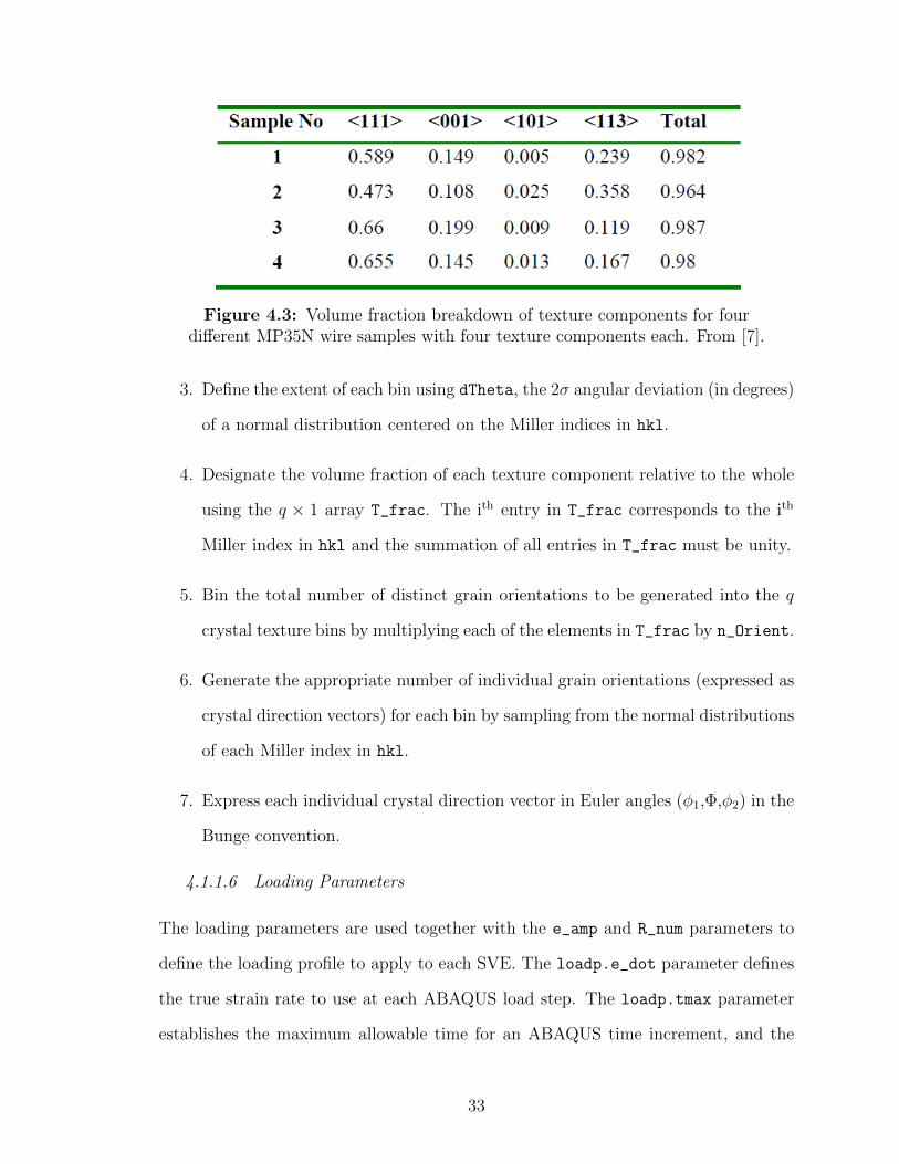
Figure 4.3: Volume fraction breakdown of texture components for fourdifferent MP35N wire samples with four texture components each. From [7].
3. Define the extent of each bin using dTheta, the 2σ angular deviation (in degrees)
of a normal distribution centered on the Miller indices in hkl.
4. Designate the volume fraction of each texture component relative to the whole
using the q × 1 array T_frac. The ith entry in T_frac corresponds to the ith
Miller index in hkl and the summation of all entries in T_frac must be unity.
5. Bin the total number of distinct grain orientations to be generated into the q
crystal texture bins by multiplying each of the elements in T_frac by n_Orient.
6. Generate the appropriate number of individual grain orientations (expressed as
crystal direction vectors) for each bin by sampling from the normal distributions
of each Miller index in hkl.
7. Express each individual crystal direction vector in Euler angles (φ1,Φ,φ2) in the
Bunge convention.
4.1.1.6 Loading Parameters
The loading parameters are used together with the e_amp and R_num parameters to
define the loading profile to apply to each SVE. The loadp.e_dot parameter defines
the true strain rate to use at each ABAQUS load step. The loadp.tmax parameter
establishes the maximum allowable time for an ABAQUS time increment, and the
33
loadp.e_yield parameter provides the 0.2% offset yield strain as obtained from
tensile tests. Unlike the DoE parameters, the Load parameters remain unchanged
between successive SVEs.
4.1.2 Instantiation of Statistical Volume Elements
An SVE is instantiated by generating a block of tetrahedral mesh containing an NMI
surrounded by a crystal-plasticity region. The crystal plasticity region is subsequently
packed with ellipsoidal grains by assigning distinct materials to ellipsoidal element
subsets of the CP region. The location, size, semi-axes ratios and physical orientation
of these ellipsoids are controlled by an ellipsoidal grain packing algorithm. This
algorithm was developed by Przybyla [15] and modified to work with tetrahedral
elements. A cut-section view of an exemplary microstructure instantiation is shown
in Figure 4.4. The grain packing algorithm consists of the following steps:
1. Determine the number of grains to pack. The total number of grains
packed depends on the size of the SVE and the grain size distribution estab-
lished.
2. Assign a target volume to each ellipsoidal grain. The target volume
of each ellipsoid is obtained by converting the grain diameter value sampled
from the experimental grain diameter distribution. The conversion equation is
Vtarget = 4π3
(dgrn2
)3.
3. Scale each target volume to a packing volume. The target volume is the
idealized volume for the completely packed SVE. It is impossible to perfectly
pack a volume with ellipsoids without overlap. Therefore each volume is scaled
down by a factor to account for imperfect packing.
4. Sort the list of ellipsoid grain volumes in descending order. For greatest
packing efficiency, the largest ellipsoid is packed first.
34

Figure 4.4: Cut-section view of an exemplary microstructure instantiationwith 1000 grains. Grains are delineated by color. The cuboidal TiN NMI
particle is shown in grey in the center. The width of the NMI is 4 µm and theSVE is 20 µm on each side.
5. Assign ellipsoid shapes. Ellipsoid morphologies are defined by the semi-axis
ratios b/c and c/a. These axes ratios are sampled from a beta distribution which
is a best estimate of MP35N grain morphology since experimental grain aspect
ratio data was unavailable. The beta distribution parameters are discussed in
Sec 4.1.1.4.
6. Assign crystal orientation. Each grain is assigned a set of Euler angles in
Bunge convention (φ1,Φ, φ2) based on the output of the texture generation algo-
rithm in section 4.1.1.5 defining the crystals rotation from the global coordinate
axes. This is unrelated to the semi-axes orientation.
35

7. Seed an ellipsoid into the SVE. Ellipsoids are placed in decreasing order of
volume to maximize packing efficiency. A random seed point (X0, Y0, Z0) within
the bounds of the SVE is chosen as the ellipsoid centroid. At the same time, a
random orientation of the semi-axes is picked.
8. Check for grain overlap. The newly placed ellipsoid must not overlap with
any previously packed grains. To check this, it is required that every element
within the ellipsoid boundary Rb is unassigned. If overlap occurs, a new random
seed point is chosen.
9. Assign elements to current grain. If no elements within Rb are previously
assigned, the space is available. All elements inside Rb are assigned to the
current grain.
10. Repeat steps 7-9 until all ellipsoids have been placed or the jamming limit
is reached. The jamming limit sets the number of grain placement attempts
allowed for a single grain. If this limit is reached and not all grains have been
placed, the algorithm quits because not enough empty space remains to finish
grain placement.
11. Grow grains until all CP elements are assigned. At this point, all ellip-
soids have been placed, but some unassigned elements remain between them.
To fill the SVE volume, these remaining elements are assigned to their nearest
grains. In this way, the grains ”grow” uniformly to fill the SVE.
A 2-dimensional illustration of the grain placement scheme, and associated coor-
dinate systems used is shown in Figure 4.5. As long as the element centroid falls
within the ellipsoid boundary Rb, it is considered to belong to the current grain.
As stated, the grain packing algorithm attempts to match an experimental grains
size distribution. Because of the domain discretization imposed by the finite element
36
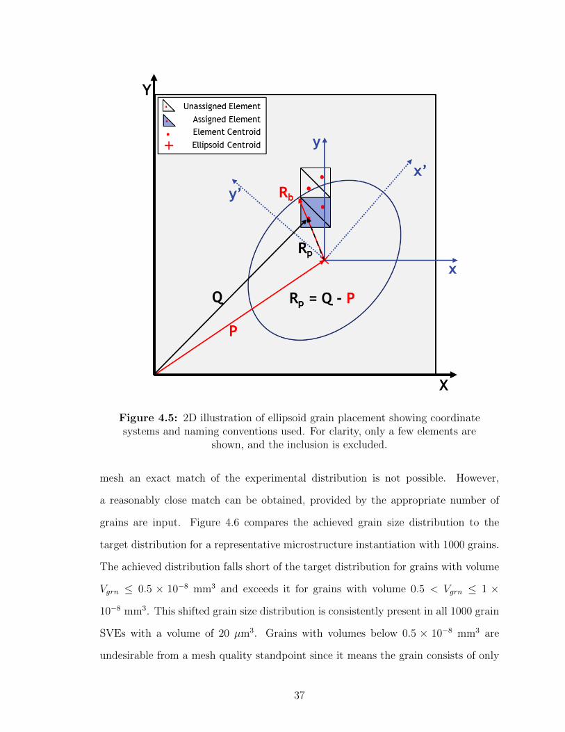
Figure 4.5: 2D illustration of ellipsoid grain placement showing coordinatesystems and naming conventions used. For clarity, only a few elements are
shown, and the inclusion is excluded.
mesh an exact match of the experimental distribution is not possible. However,
a reasonably close match can be obtained, provided by the appropriate number of
grains are input. Figure 4.6 compares the achieved grain size distribution to the
target distribution for a representative microstructure instantiation with 1000 grains.
The achieved distribution falls short of the target distribution for grains with volume
Vgrn ≤ 0.5 × 10⁻⁸ mm3 and exceeds it for grains with volume 0.5 < Vgrn ≤ 1 ×
10−8 mm3. This shifted grain size distribution is consistently present in all 1000 grain
SVEs with a volume of 20 µm3. Grains with volumes below 0.5 × 10⁻⁸ mm3 are
undesirable from a mesh quality standpoint since it means the grain consists of only
37

a handful of elements.
Figure 4.6: PDF of a representative microstructure instantiation with 1000grains comparing the achieved grain size distribution to the target distribution.
Grain morphology of the ellipsoids are specified by the ratios b/a and c/a, where
a, b, c are the semi-axes of the ellipsoid, satisfying a > b > c. These axes ratios
are taken from a beta distribution which is a best estimate of actual MP35N grain
aspect ratios since experimental grain aspect ratio data is not available. The values
of the shape parameters α and β used in the beta distribution are listed in Table
4.1. A point cloud of the targeted semi-axes ratios from an exemplary 1000 grain
microstructure instantiation is presented in Figure 4.7. All points lie below the line
b/a = c/a since b > c in all cases. Actual semi-axes ratios may deviate slightly from
the targets due to the grain growth step.
4.1.3 Mesh Quality Study
The finite element mesh utilized in this model is comprised of linear tetrahedral con-
tinuum elements (C3D4). These elements permit mesh refinement around areas of
38
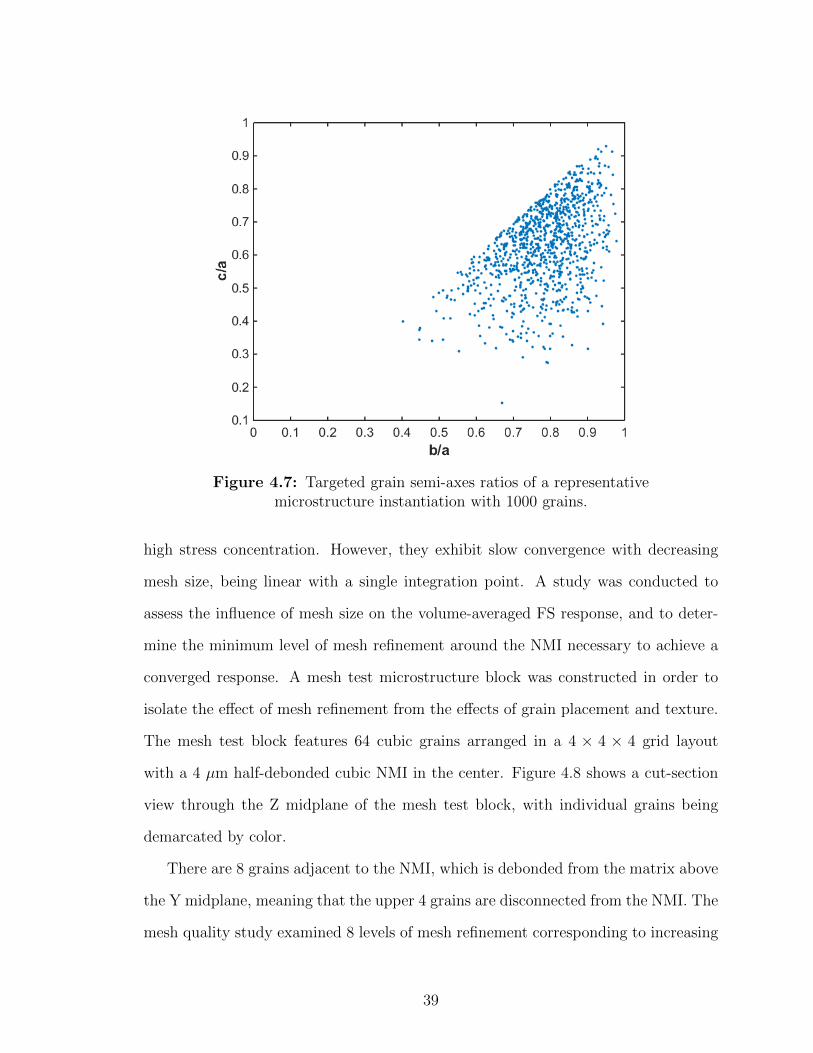
Figure 4.7: Targeted grain semi-axes ratios of a representativemicrostructure instantiation with 1000 grains.
high stress concentration. However, they exhibit slow convergence with decreasing
mesh size, being linear with a single integration point. A study was conducted to
assess the influence of mesh size on the volume-averaged FS response, and to deter-
mine the minimum level of mesh refinement around the NMI necessary to achieve a
converged response. A mesh test microstructure block was constructed in order to
isolate the effect of mesh refinement from the effects of grain placement and texture.
The mesh test block features 64 cubic grains arranged in a 4 × 4 × 4 grid layout
with a 4 µm half-debonded cubic NMI in the center. Figure 4.8 shows a cut-section
view through the Z midplane of the mesh test block, with individual grains being
demarcated by color.
There are 8 grains adjacent to the NMI, which is debonded from the matrix above
the Y midplane, meaning that the upper 4 grains are disconnected from the NMI. The
mesh quality study examined 8 levels of mesh refinement corresponding to increasing
39

Figure 4.8: Cut-section view of SVE generated for mesh quality studyshowing 64 cubic grains and central NMI.
the number of elements along the NMI edge. Table 4.2 shows the mesh densities,
model size and run times for each of the 8 mesh density levels. The model size is the
total number of elements present in the model and is the sum of the matrix and NMI
elements. All mesh instantiations are evaluated over the third fully-reversed tension-
compression cycle with a loading amplitude of 0.55 εy to ensure non-zero plastic strain
values within the FS AVs. Grains retain the same position, size and crystal orientation
for all mesh density levels.
The mesh is most dense at the NMI edge and gradually becomes coarser towards
the SVE boundary. As the number of elements along the NMI increases, the model
size also increases, resulting in an increase in the run time. Figure 4.9 shows the
time to run the model for increasing mesh density. The models were run in a Linux
40

Table 4.2: Summary of size and run-time measures for the eight mesh density levels
Mesh Density Level ElementsalongNMIEdge
ElementsalongSVEEdge
ModelSize
MatrixModelSize
RunTime(s)
1 9 12 27,924 24,880 1,513
2 11 12 34,951 29,987 1,924
3 13 16 62,235 54,054 3,533
4 15 16 78,184 66,871 4,585
5 17 16 89,012 73,718 5,204
6 19 16 99,395 79,122 7,140
7 21 20 144,947 120,027 11,193
8 25 20 169,320 131,036 21,935
high-performance computing environment utilizing parallel processing on a total of 40
CPUs. A mesh density of 17 elements along the NMI can be considered a transitional
value for computational efficiency. Above this value, the run-time begins to increase
rapidly, while below it the run-time increases slowly and stays below 5000 seconds.
Based on this data, it is seen that higher computational efficiency is achieved using
a mesh density at or below 17 elements along the NMI edge, so long as the volume-
averaged FS values using that mesh density can be considered converged.
Convergence of FS values can be evaluated by comparing the change in FS values
as mesh density is increased. Figure 4.10 shows the FS response of the Full-Face AV
along the X−, X+, Z−, Z+ NMI faces against the number of elements along the NMI
edge which can be thought of as the linear element density. The AV located along the
Z− face showed an elevated FS response compared to the other three faces, due to
higher levels of plasticity resulting from grains oriented favorably for slip. The other
three face volumes have nearly identical response values to one another. The Z−
Face AV and the others share a similar response profile as mesh density is increased,
41

Figure 4.9: Run-time (in seconds) for increasing number of elements alongNMI edge.
however the profile is exaggerated for the Z− Face AV due to the intensified FS
response there. Between 9 and 11 the FS response is essentially unchanged. From 11
to 15, the FS response increases sharply by 50% from 0.8×10⁻³ to 1.2×10⁻³. Above
15, the FS response value stabilizes, rising only 13% over a linear element density
increase of 10. Based on this analysis, the FS response for the Full-Face AVs were
considered converged at a linear NMI density of 15 elements.
The FS value convergence response was also checked on the Mid AV to confirm
the smaller AVs with one-half NMI width behaved similarly. Figure 4.11 shows the
FS response of the Mid AV along each of the X−, X+, Z−, Z+ NMI faces, plotted
on the same axes as Figure 4.10. The Z− Mid-Face AV response has been translated
upward by roughly 0.2× 10⁻³ compared to the Z- Full-Face AV while maintaining a
similar profile shape. As in Figure 4.10, the FS response value rises between 11 to
42

Figure 4.10: Volume-averaged Full-Face FS response for increasing numberof elements along NMI edge.
15 and flattens out at higher densities. The other three Mid-Face AVs responses are
nearly unchanged compared to their Full-Face counterparts. Because of this, a mesh
density of 15 elements along the NMI edge was the mesh density selected for use in
further studies, being the minimum mesh density needed for converged FS response
values.
43

Figure 4.11: Volume-averaged Mid-Face FS response for increasing numberof elements along NMI edge.
44

Table
4.3
:V
aria
ble
s,par
amet
ers
and
coeffi
cien
tsuse
din
const
ituti
vere
lati
ons
Typ
eN
am
eSym
bol
UM
AT
equiv
ale
nt
Desc
ripti
on
ind
exsl
ip-s
yst
emα
nor
kC
ryst
alsl
ip-s
yst
emid
enti
fier
.R
ange
sfr
om1-
12fo
roct
ahed
ral
syst
ems.
vari
able
shea
rst
rain
rate
γgamma_dot
Inel
asti
csh
ear
stra
inra
te
coeff
.sh
ear
rate
coeff
.γo
gamma_dot_zero
Inel
asti
csh
ear
stra
inra
teco
effici
ent
vari
able
reso
lved
shea
rst
ress
τtau
Res
olve
dsh
ear
stre
ss.
vari
able
bac
kst
ress
χa
Inte
rnal
,kin
emat
icst
ress
wh
ich
resu
lts
from
pil
e-u
pof
dis
loca
tion
sal
ong
grai
nor
oth
erb
oun
dar
ies.
vari
able
thre
shol
dst
ress
κg
Isot
rop
icst
ress
that
contr
ols
the
onse
tof
inel
asti
cd
efor
mat
ion
.
phys.
par
am.
dra
gst
ress
Dd
Str
ess
gove
rnin
gin
tern
alre
sist
ance
top
last
icfl
ow.
phys.
par
am.
flow
exp
onen
tn
flow_exp1
Exp
onen
tgo
vern
ing
the
mat
eria
lst
rain
-rat
ese
nsi
tivit
y.
phys.
par
am.
init
ial
thre
shol
dst
ress
κo
tau_0
Init
ial
thre
shol
dst
ress
valu
e.
coeff
.d
islo
cati
onar
ran
gem
ent
coeffi
cien
tαt
alpha
Coeffi
cien
tto
acco
unt
for
dis
loca
tion
arra
nge
men
tin
mic
rost
ruct
ure
.
phys.
par
am.
shea
rm
od
ulu
sµ
pmeu_matrix
Sh
ear
mod
ulu
sof
MP
35N
.
phys.
par
am.
Bu
rger
’sve
ctor
bc_b
Bu
rger
’sve
ctor
mag
nit
ud
efo
rM
P35
N.
vari
able
dis
loca
tion
den
sity
ρrho
Dis
loca
tion
den
sity
ona
give
nsl
ip-s
yst
em.
45

4.2 Constitutive Model Parameter Fitting
The parameters of the constitutive model outlined in Sec 3.2 were calibrated using a
combination of existing values from literature, first principles calculations, and itera-
tive fitting against cyclic mechanical test data. The material response is a function of
both the parameter values and the crystallographic texture of the microstructure, so
the parameter fits must be adjusted for significant changes in texture. Three distinct
model calibrations were performed: an initial calibration that was a first-order ap-
proximation targeting a microstructure with a single texture distribution around the
〈111〉, an intermediate calibration to improve the kinematic hardening response and
a revised calibration targeting a microstructure with multiple texture components in
the 〈001〉, 〈113〉 and 〈111〉. The parameter fitting for the initial, intermediate and
revised calibrations as well as the calibration experiments undertaken are described
in the following sections.
4.2.1 Calibration Experiments
Data from two main calibration experiments was collected on MP35N fine wire in
order to appropriately fit the constitutive model parameters to the material response
behavior. In order to calibrate the isotropic hardening behavior and the strain-rate
sensitivity, uniaxial tensile test data was collected from [14]. This test was conducted
on a 10 in length of low-Ti as-drawn MP35N wire in displacement control alternating
every 0.5% strain between high and low strain rates of 1.7× 10⁻³ and 1.7× 10⁻⁵ s−1
respectively. Figure 4.12 shows the stress-strain plot for the so-called strain-rate jump
test illustrating the jump test. The sensitivity of the stress response to the strain rate
becomes evident beyond 1% strain when the wire response is no longer purely elastic.
The parameters governing the kinematic hardening behavior were determined by
fitting to the model to cyclic tension-tension experiments. Two 10 in lengths of
low-Ti MP35N as-drawn wire were cycled in load control for 10,000 cycles under a
46

Figure 4.12: Strain-rate jump test on low-Ti MP35N as-drawn wire withstrain rate alternating every 0.5% increment of strain. From [14].
R = SminSmax
= 0.5 load ratio. The tests had different maximum stress values of Smax1 =
1400 MPa and Smax2 = 1500 MPa referred to as LCF1 and LCF2, respectively. After
hundreds of cycles, the difference in accumulated strain between the two tests caused
by the non-zero mean stress could be compared to determine the increment of strain
over each cycle. Figure 4.13 shows the results of the first 300 cycles of each test.
The total accumulated strain for LCF 2 is larger than for LCF 1. To determine
the rate of plastic strain accumulation, the peak strain values for LCF 1 are plotted
against the base-10 log of cycles log(N) as shown in Figure 4.14. Each data point is
the peak strain over a single cycle. The rate of strain accumulation stabilizes to a
logarithmic relationship after ten cycles. A similar logarithmic fit was calculated for
LCF 2. The difference in strain accumulation between LCF 1 and LCF 2 was used
to calibrate the backstress evolution parameters.
47

Figure 4.13: Strain Ratcheting Experiments showing the accumulation ofstrain over 300 cycles for Smax
1 = 1400 MPa and Smax2 = 1500 MPa.
Figure 4.14: Plot of log(N) vs peak strain (mm/mm) for the LCF1experiment. The rate of strain accumulation stabilizes after 10 cycles.
48

4.2.2 Initial Parameter Calibration
The initial model calibration was a first order estimate targeting a microstructure with
a single texture component distribution around the 〈111〉 orientation. The parameter
values for the initial calibration are given in Table 4.4.
Table 4.4: Values of the constitutive parameters for the initial model calibration(UMAT v28)
C11 C12 C44 γo n Do τo ρo
179,789(MPa)
89,485(MPa)
70,285(MPa)
6.1× 10¹⁶
(s−1)15 150
(MPa)85.15(MPa)
7.0×10⁹
(mm−2)
αt µ b nk cgr dgr ftw
0.1 70,285(MPa)
0.407(nm)
1 9.432(MPa
√mm)
0.002(mm)
0.1
Cχ ηo t ho k1 k2 k3
2 2.82 0.0001(mm)
0.4 100,000(mm−1)
3.162 0.1
Parameters n, Do, τo, αt, b, nk, cgr, Cχ, ηo and ho are unchanged from the values
in [21] used for IN100. The values of these parameters for MP35N are expected
to be similar to those for IN100, since both are fcc alloys containing significant Ni
content. Parameters dgr, ftw, t and k3 were added to account for the strengthening
effect of the small grain size and nano-scale twins. The value of dgr was set to the
median grain size of 2 µm and t was given a value of 10 nm consistent with the twin
spacing revealed by TEM [14, 23]. The values of ftw and k3 were chosen to reflect
physically reasonable values. The shear strain rate coefficient γo is set to 6.1×10¹⁶ s−1.
The initial dislocation density ρo was given a value of 7.0 × 109 mm2 reflecting the
high initial dislocation density from 36% cold work in the as-drawn MP35N wire.
Additional cyclic deformation from fatigue type loading is not expected to further
increase ρ, so the ratio of k1 and k2 is selected such that ρ saturates above ρo.
The values of the elastic parameters C11, C12 and C44 needed for the 4th rank
49
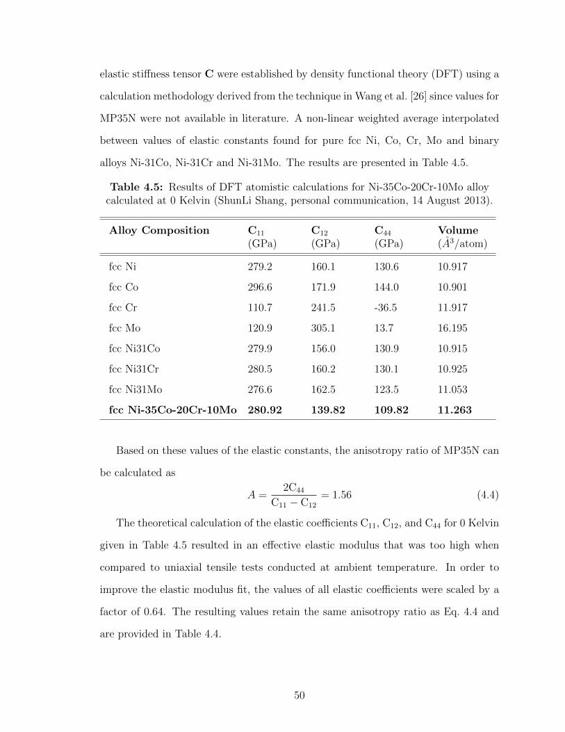
elastic stiffness tensor C were established by density functional theory (DFT) using a
calculation methodology derived from the technique in Wang et al. [26] since values for
MP35N were not available in literature. A non-linear weighted average interpolated
between values of elastic constants found for pure fcc Ni, Co, Cr, Mo and binary
alloys Ni-31Co, Ni-31Cr and Ni-31Mo. The results are presented in Table 4.5.
Table 4.5: Results of DFT atomistic calculations for Ni-35Co-20Cr-10Mo alloycalculated at 0 Kelvin (ShunLi Shang, personal communication, 14 August 2013).
Alloy Composition C11
(GPa)C12
(GPa)C44
(GPa)Volume(A3/atom)
fcc Ni 279.2 160.1 130.6 10.917
fcc Co 296.6 171.9 144.0 10.901
fcc Cr 110.7 241.5 -36.5 11.917
fcc Mo 120.9 305.1 13.7 16.195
fcc Ni31Co 279.9 156.0 130.9 10.915
fcc Ni31Cr 280.5 160.2 130.1 10.925
fcc Ni31Mo 276.6 162.5 123.5 11.053
fcc Ni-35Co-20Cr-10Mo 280.92 139.82 109.82 11.263
Based on these values of the elastic constants, the anisotropy ratio of MP35N can
be calculated as
A =2C44
C11 − C12
= 1.56 (4.4)
The theoretical calculation of the elastic coefficients C11, C12, and C44 for 0 Kelvin
given in Table 4.5 resulted in an effective elastic modulus that was too high when
compared to uniaxial tensile tests conducted at ambient temperature. In order to
improve the elastic modulus fit, the values of all elastic coefficients were scaled by a
factor of 0.64. The resulting values retain the same anisotropy ratio as Eq. 4.4 and
are provided in Table 4.4.
50

4.2.3 Intermediate Parameter Calibration
An intermediate calibration was undertaken to improve isotropic and kinematic hard-
ening behavior of the model to the monotonic tensile and cyclic tension-tension tests.
Several parameters were adjusted from the initial fit of Table 4.4 including γo, n,
Do, τo, ρo, ηo and the elastic constants. The adjusted parameter values used in the
intermediate calibration are given in Table 4.6. Comparisons of the model fits using
the initial and intermediate model calibrations against the strain-rate jump and LCF
1 experiments are provided in Figures 4.15 and 4.16, respectively. In these plots, the
terms ”original” and ”latest” refer to the initial and intermediate parameter calibra-
tions.
Table 4.6: Values of the constitutive parameters for the intermediate modelcalibration (UMAT v110)
C11 C12 C44 γo n Do τo ρo
165,406(MPa)
82,326(MPa)
64,662(MPa)
7.2× 10¹⁶
(s−1)18 195
(MPa)75.15(MPa)
3.0×10⁹
(mm−2)
αt µ b nk cgr dgr ftw
0.1 64,662(MPa)
0.407(nm)
1 9.432(MPa
√mm)
0.002(mm)
0.1
Cχ ηo t ho k1 k2 k3
2 68.0 0.0001(mm)
1 100,000(mm−1)
1.0 0.1
An increase of the flow exponent n from 15 to 18 improves the rate sensitivity
of the model as evidence by the deeper trough features in the ”latest” model fit.
The amount of isotropic hardening seen post-yield is also increased by enhancing the
value of ηo to better reflect the experiment. The value of the elastic coefficients C11,
C12 and C44 are reduced proportionately from the initial fit, resulting in a poorer
fit of the elastic portion of the curve. This reduction was a compromise in order to
better fit the cyclic value of the elastic modulus in Fig 4.16. In this plot, the first
51
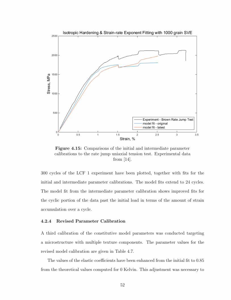
Figure 4.15: Comparisons of the initial and intermediate parametercalibrations to the rate jump uniaxial tension test. Experimental data
from [14].
300 cycles of the LCF 1 experiment have been plotted, together with fits for the
initial and intermediate parameter calibrations. The model fits extend to 24 cycles.
The model fit from the intermediate parameter calibration shows improved fits for
the cyclic portion of the data past the initial load in terms of the amount of strain
accumulation over a cycle.
4.2.4 Revised Parameter Calibration
A third calibration of the constitutive model parameters was conducted targeting
a microstructure with multiple texture components. The parameter values for the
revised model calibration are given in Table 4.7.
The values of the elastic coefficients have been enhanced from the initial fit to 0.85
from the theoretical values computed for 0 Kelvin. This adjustment was necessary to
52

Figure 4.16: Comparisons of the initial and intermediate parametercalibrations to the LCF1 strain ratcheting experiment.
Table 4.7: Values of the constitutive parameters for the revised model calibration(UMAT v110e)
C11 C12 C44 γo n Do τo ρo
237,321(MPa)
118,120(MPa)
92,756(MPa)
7.2× 10¹⁶
(s−1)18 195
(MPa)75.15(MPa)
3.0×10⁹
(mm−2)
αt µ b nk cgr dgr ftw
0.1 92,756(MPa)
0.407(nm)
1 9.432(MPa
√mm)
0.002(mm)
0.1
Cχ ηo t ho k1 k2 k3
2 68.0 0.0001(mm)
1 100,000(mm−1)
1.0 0.1
correct for the inherent reduction in elastic stiffness from reduced volume fraction of
53

〈111〉 texture. The sensitivity of the effective elastic modulus to changes in crystal-
lographic texture can be seen from Fig 4.17 which plots the results of the rate jump
test run on a 1000 grain SVE for pure 〈111〉, pure 〈001〉 and mixed texture using the
intermediate fit of the elastic constants found in Table 4.6.
Figure 4.17: Sensitivity of the effective elastic modulus to SVE texture.
The material stiffness is highest for a pure 〈111〉 crystallographic texture, and
reduces as the volume fraction of 〈111〉 is reduced to zero.
54

CHAPTER V
RESULTS AND DISCUSSION
5.1 FIP-Life Correlations
Several studies were undertaken using the newly developed CPFEM model in order
to assess its efficacy for generating fatigue-life correlations in MP35N fine wires. The
model results were compared to MP35N fatigue data available in literature and are
presented in this chapter.
5.1.1 Effect of Inclusion Proximity to Surface
A parametric study was conducted to investigate the ability of the model to predict
the effect of NMI surface proximity on fatigue life. The aim of the study was to
replicate the inclusion surface proximity versus fatigue life trend of Full-Ti MP35N
wire as demonstrated experimentally by the solid trend line in Figure 2.9. A Virtual
Design of Experiments (VDoE) was created with four levels Li corresponding to
different NMI distances from the wire surface. Twenty microstructure instantiations
were run at each level, in order to estimate the median fatigue life and scatter.
Each microstructure instantiation is a 20 µm3 SVE occupying a volume immedi-
ately adjacent to the outer surface of the MP35N wire. The positive X-face is along
the wire outer surface, and all other SVE faces are interior. Periodic boundary con-
ditions are prescribed for the Y and Z faces and all edges. The positive X-face is
traction-free and unconstrained, while the negative X-face is given a node-wise dis-
placement boundary condition to mimic a periodic boundary. The negative X-face
displacement boundary conditions are extracted from a reference analysis having fully
3D boundary conditions but identical mesh and loading history.
Each SVE was instantiated with 1000 grains according to the ellipsoid packing
55

method described in Sec 4.1.2. The grains were given a fiber texture with a single
texture component normally distributed about the 111 orientation with standard
deviation defined such that 2σ = 15. The full set of constitutive parameter values
used in the study are given in Table 4.4.
The NMI distance from the wire surface xsurf was defined as the perpendicular
distance from the wire surface to the nearest point of the NMI. Similarly, the centroid
distance xc was defined as the perpendicular distance from the wire surface to the
NMI centroid. These and other geometry parameters for the NMI are illustrated in
Figure 5.1. NMI size was fixed at 4 µm for all VDoE levels. The NMIs were oriented
such that the inclusion faces were parallel to the SVE faces. All NMIs had their upper
halves debonded from the matrix, as described in Sec 3.3.2. Values of the parameters
relating to the NMI position at each level of the VDoE are given in Table 5.1.
Figure 5.1: Subset of an SVE showing definitions of TiN particle geometryas related to the wire surface.
The loading profile applied to each microstructure instantiation was in the form
of three fully-reversed R = −1 displacement controlled cycles. Figure 5.2 shows the
form of the loading profile applied to the SVEs. This history is intended to replicate
56
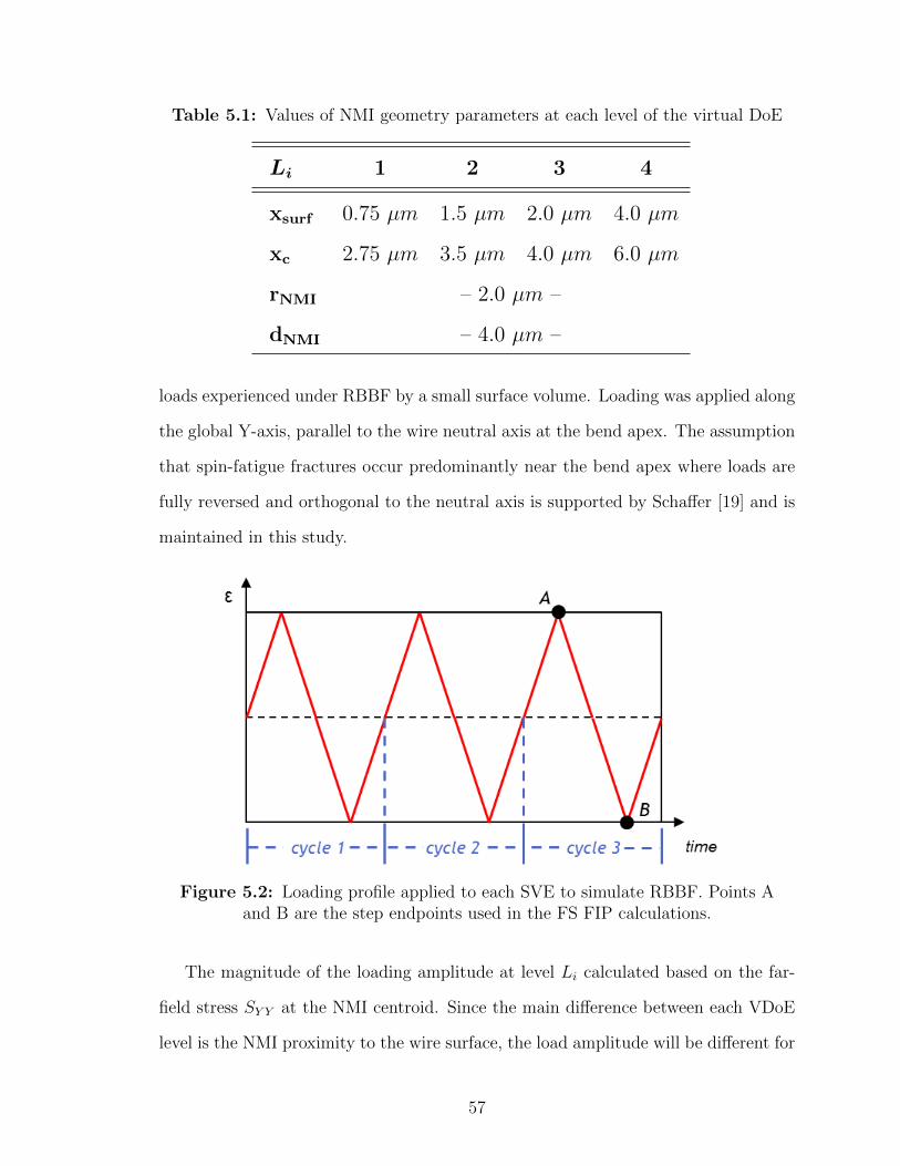
Table 5.1: Values of NMI geometry parameters at each level of the virtual DoE
Li 1 2 3 4
xsurf 0.75 µm 1.5 µm 2.0 µm 4.0 µm
xc 2.75 µm 3.5 µm 4.0 µm 6.0 µm
rNMI – 2.0 µm –
dNMI – 4.0 µm –
loads experienced under RBBF by a small surface volume. Loading was applied along
the global Y-axis, parallel to the wire neutral axis at the bend apex. The assumption
that spin-fatigue fractures occur predominantly near the bend apex where loads are
fully reversed and orthogonal to the neutral axis is supported by Schaffer [19] and is
maintained in this study.
Figure 5.2: Loading profile applied to each SVE to simulate RBBF. Points Aand B are the step endpoints used in the FS FIP calculations.
The magnitude of the loading amplitude at level Li calculated based on the far-
field stress SY Y at the NMI centroid. Since the main difference between each VDoE
level is the NMI proximity to the wire surface, the load amplitude will be different for
57

each level. The far-field stress parallel to neutral axis of a wire in rotating bending is
a strong function of the depth x beneath the wire surface. At the outer fiber, SY Y is
a maximum, equal to the stress amplitude Sa in Eq. 2.3. At the neutral axis SY Y is
zero. In general, neglecting microstructural inhomogeneity, the far-field stress SY Y is
a linear function of depth x beneath the wire surface, expressed as
SY Y (x) = − Sarwire
(x) + Sa (5.1)
where rwire is the radius of the wire undergoing RBBF, and the quantity − Sarwire
is the
far-field stress gradient along the x-axis. In the ideal case, the SVE would be loaded
with a linearly varying load along X as described by Eq. 5.1. However, non-uniform
loads are incompatible with periodic boundary conditions due to the need to drive
displacement boundary conditions from a single reference node. In order to maintain
periodic boundary conditions while matching the stress state in the region of interest
as closely as possible, the displacement on the reference node was determined by
conversion from the far-field stress at the NMI centroid. This value was computed by
inputting the appropriate value of xc for each level Li of the VDoE, such that
SLiY Y = − Sarwire
(xLic ) + Sa (5.2)
The far-field stress value determined for each level was converted into a strain ampli-
tude and then to displacement amplitude by
εa =SLiY YE
(5.3)
and
Ya = 20 µm · εa (5.4)
with E being the elastic modulus of the MP35N wire and 20 µm being the length
dimension of an SVE along the loading axis. This step was taken to closely match
58

of the far-field stresses in the FS AVs positioned along the NMI debond perimeter to
the actual localized stresses generated by the RBBF experiments. Table 5.2 presents
the relationships between the beam-bending stress amplitude at the wire apex, NMI
surface proximity and SVE applied stress and strain amplitudes for the VDoE.
Table 5.2: Relationships between beam-bending stress reported at the wire apex(Sa) and stress (SY Y ) and strain (εa) amplitudes applied to the SVE
Li xsurf
(µm)Sa
(MPa)SY Y
(MPa)εa(% of εy)
1 0.75 620 586 0.331
2 1.5 620 577 0.325
3 2.0 620 570 0.322
4 4.0 620 546 0.308
The fidelity near the NMI comes at the expense of accuracy far from the NMI
centroid along the X axis, but this is considered acceptable since the material response
in these regions does not enter into the FS calculations. Figure 5.3 shows how the
SVE stress amplitude used in the study compares to the SY Y stress gradient between
the outer surface and the neutral axis.
Twenty microstructure instantiations were run at each of the four NMI depths
0.75, 1.5, 2.0 and 4.0 µm. The maximum volume-averaged FS parameter was com-
puted for each run as described in Sec 3.3.1 and Sec 3.3.2. Figure 5.4 shows the EV
FS values plotted against NMI distance from surface.
The EV FS values plotted in Figure 5.4 were correlated to fatigue life values
through the Modified Tanaka-Mura approach from Sec 3.5. The correlation to life
was performed at the 0.75 µm level assuming negligible propagation life. The median
EV FS value was correlated to the linear regression fit the experimental data points
with dgr = 1.5 µm. A correlation coefficient α = 1.129×10⁻⁵ µm–cycles was found to
59

Figure 5.3: Selection of stress amplitude for an SVE. Stress amplitude SY Ydecreases linearly with NMI depth xc due to the stress gradient generated in
bending. Note that the x axis for depth is opposite the global X axis.
correlate well to experiment. The three remaining VDoE levels were correlated using
the same values of α and dgr. The resulting life-correlations are plotted against the
experimental data points in Figure 5.5.
As expected, the life-correlation results show increasing life values as the NMI
depth from the free surface is increased. Moreover, the model results show good over-
lap with the linear regression trend computed from the experimental data points at all
depths considered in the VDoE. The minimum lives predicted by the model at each
level is below the 5% confidence bound. This indicates that the model gives a more
conservative prediction of minimum fatigue life than the regression fit. The accuracy
60
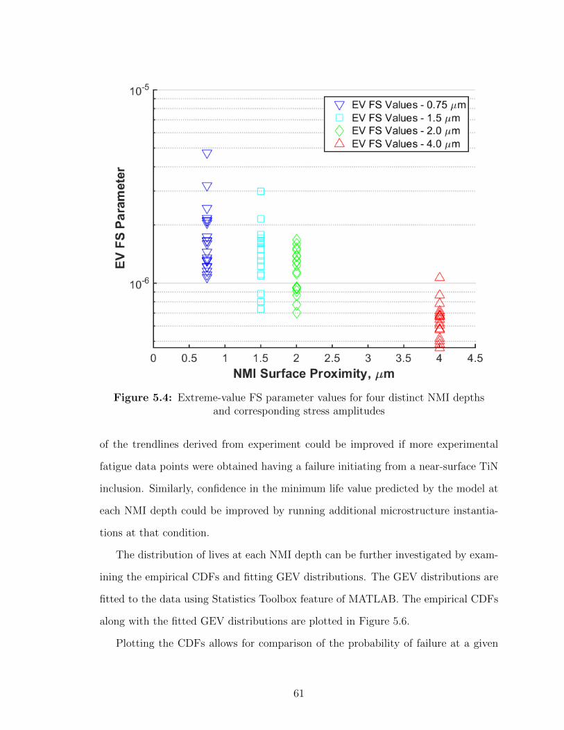
Figure 5.4: Extreme-value FS parameter values for four distinct NMI depthsand corresponding stress amplitudes
of the trendlines derived from experiment could be improved if more experimental
fatigue data points were obtained having a failure initiating from a near-surface TiN
inclusion. Similarly, confidence in the minimum life value predicted by the model at
each NMI depth could be improved by running additional microstructure instantia-
tions at that condition.
The distribution of lives at each NMI depth can be further investigated by exam-
ining the empirical CDFs and fitting GEV distributions. The GEV distributions are
fitted to the data using Statistics Toolbox feature of MATLAB. The empirical CDFs
along with the fitted GEV distributions are plotted in Figure 5.6.
Plotting the CDFs allows for comparison of the probability of failure at a given
61
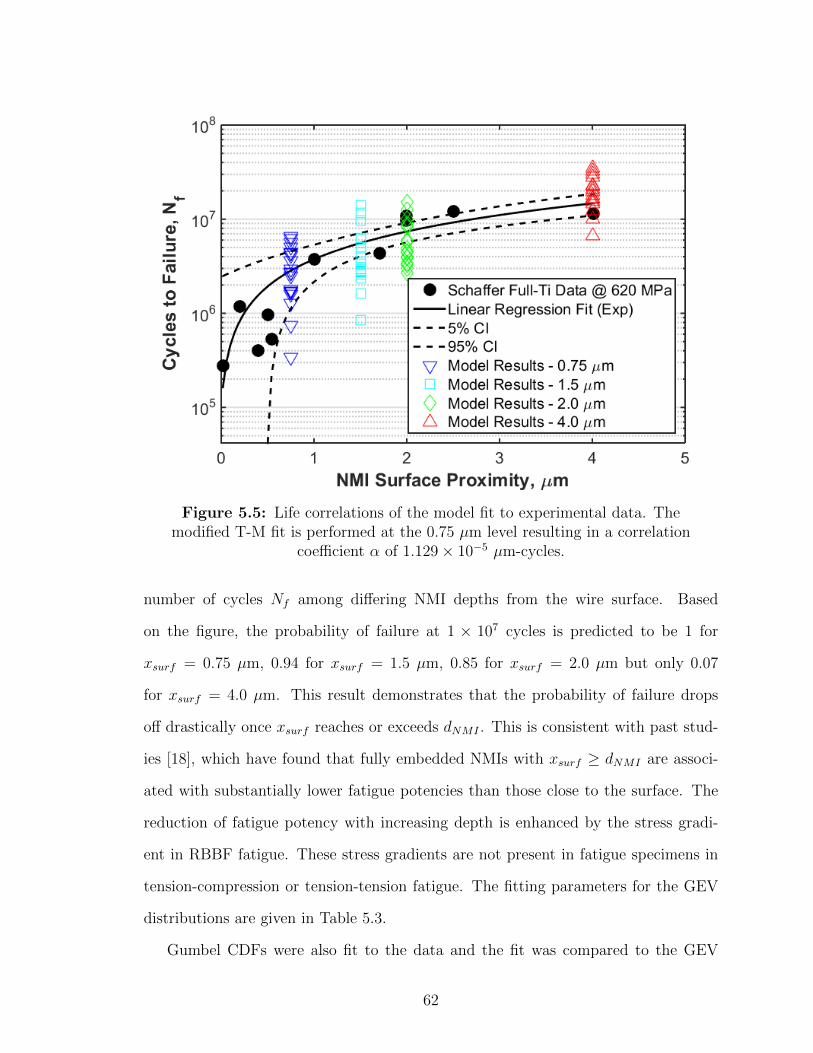
Figure 5.5: Life correlations of the model fit to experimental data. Themodified T-M fit is performed at the 0.75 µm level resulting in a correlation
coefficient α of 1.129× 10⁻⁵ µm-cycles.
number of cycles Nf among differing NMI depths from the wire surface. Based
on the figure, the probability of failure at 1 × 10⁷ cycles is predicted to be 1 for
xsurf = 0.75 µm, 0.94 for xsurf = 1.5 µm, 0.85 for xsurf = 2.0 µm but only 0.07
for xsurf = 4.0 µm. This result demonstrates that the probability of failure drops
off drastically once xsurf reaches or exceeds dNMI . This is consistent with past stud-
ies [18], which have found that fully embedded NMIs with xsurf ≥ dNMI are associ-
ated with substantially lower fatigue potencies than those close to the surface. The
reduction of fatigue potency with increasing depth is enhanced by the stress gradi-
ent in RBBF fatigue. These stress gradients are not present in fatigue specimens in
tension-compression or tension-tension fatigue. The fitting parameters for the GEV
distributions are given in Table 5.3.
Gumbel CDFs were also fit to the data and the fit was compared to the GEV
62

Figure 5.6: CDFs of the Fatigue-life correlations with corresponding GEVdistributions.
Table 5.3: Fitting Parameters for GEV CDFs
xsurf (µm) µ σ ξ Type
0.75 2.554× 10⁶ 1.679× 10⁶ −0.214 III (Weibull)
1.5 2.727× 10⁶ 1.780× 10⁶ 0.314 II (Frechet)
2.0 4.937× 10⁶ 2.250× 10⁶ 0.250 II (Frechet)
4.0 1.668× 10⁷ 6.336× 10⁶ −0.131 III (Weibull)
case. The fit is shown in Figure 5.7. By comparing to Figure 5.6, it can be seen that
the GEV CDFs give a better fit, especially at probabilities of failure from 0 to 0.2.
The Gumbel distribution fit is especially poor for xsurf = 1.5µm.
The Gumbel distributions predict no minimum life value for the values of xsurf
investigated because the CDFs approach zero probability of failure slowly as Nf
goes to zero. Table 5.4 lists the fitting parameters for the Gumbel distributions. The
63

restriction of ξ to 0 results in the poor fits to the empirical CDFs at the low likelyhood
end of the distributions.
Figure 5.7: CDFs of the fatigue-life correlations with fitted Gumbeldistributions.
Table 5.4: Fitting Parameters for Gumbel CDFs
xsurf (µm) µ σ ξ
0.75 4.163× 10⁶ 1.733× 10⁶ 0
1.5 6.394× 10⁶ 4.273× 10⁶ 0
2.0 8.600× 10⁶ 3.712× 10⁶ 0
4.0 2.337× 10⁷ 7.511× 10⁶ 0
5.1.2 Identifying the Crack Incubation to Microcrack Growth Transition
A second study was conducted to identify the transition life between fatigue crack
incubation and microcrack growth regimes using Eq. 3.12 to correlate to an additional
64
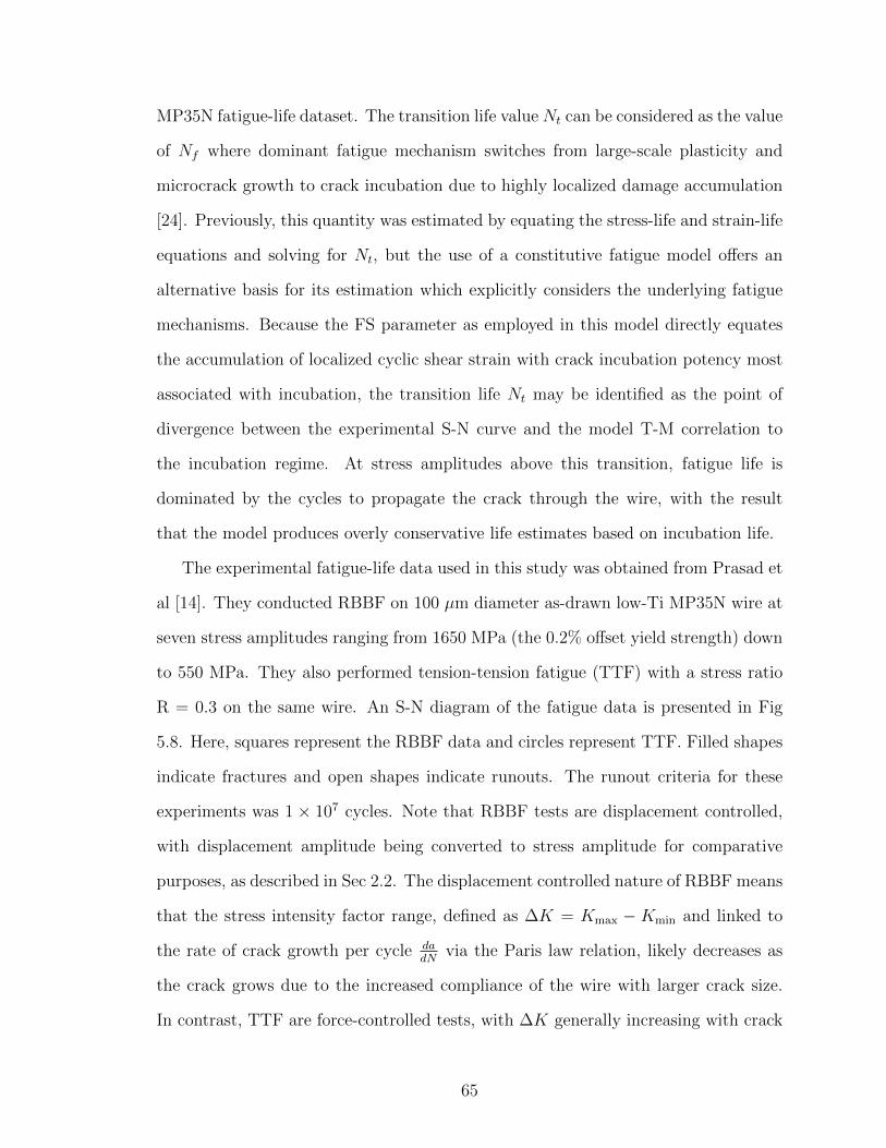
MP35N fatigue-life dataset. The transition life value Nt can be considered as the value
of Nf where dominant fatigue mechanism switches from large-scale plasticity and
microcrack growth to crack incubation due to highly localized damage accumulation
[24]. Previously, this quantity was estimated by equating the stress-life and strain-life
equations and solving for Nt, but the use of a constitutive fatigue model offers an
alternative basis for its estimation which explicitly considers the underlying fatigue
mechanisms. Because the FS parameter as employed in this model directly equates
the accumulation of localized cyclic shear strain with crack incubation potency most
associated with incubation, the transition life Nt may be identified as the point of
divergence between the experimental S-N curve and the model T-M correlation to
the incubation regime. At stress amplitudes above this transition, fatigue life is
dominated by the cycles to propagate the crack through the wire, with the result
that the model produces overly conservative life estimates based on incubation life.
The experimental fatigue-life data used in this study was obtained from Prasad et
al [14]. They conducted RBBF on 100 µm diameter as-drawn low-Ti MP35N wire at
seven stress amplitudes ranging from 1650 MPa (the 0.2% offset yield strength) down
to 550 MPa. They also performed tension-tension fatigue (TTF) with a stress ratio
R = 0.3 on the same wire. An S-N diagram of the fatigue data is presented in Fig
5.8. Here, squares represent the RBBF data and circles represent TTF. Filled shapes
indicate fractures and open shapes indicate runouts. The runout criteria for these
experiments was 1 × 10⁷ cycles. Note that RBBF tests are displacement controlled,
with displacement amplitude being converted to stress amplitude for comparative
purposes, as described in Sec 2.2. The displacement controlled nature of RBBF means
that the stress intensity factor range, defined as ∆K = Kmax − Kmin and linked to
the rate of crack growth per cycle dadN
via the Paris law relation, likely decreases as
the crack grows due to the increased compliance of the wire with larger crack size.
In contrast, TTF are force-controlled tests, with ∆K generally increasing with crack
65

growth. Because the increased rate of crack growth as well as the positive mean
stress, it is expected that the life to failure in TTF is controlled by crack formation
at all stress amplitudes and does not exhibit a crack growth dominated regime.
Figure 5.8: Prasad et al. S-N data for as-drawn low-Ti MP35N wire [14].
Comparing the RBBF and TTF fatigue data in Fig 5.8, it is seen that the TTF
life distribution is below that of the RBBF at every comparable stress amplitude.
One contributing factor is the difference in the highly stressed volume due to the
test geometry. For equivalent Smax, assuming uniform spatial defect distributions,
the likelihood of finding a fatigue hotspot with sufficient driving force to nucleate a
fatigue crack increases in proportion to the size of the highly stressed volume. A larger
highly stressed volume samples a much larger subset of the defect population within
an individual test specimen and biases the fracture initiation toward higher potency
flaws leading to earlier crack nucleation and reduced fatige life. In addition, the
likelihood of multiple cracks forming independently and later coalescing into a single
66
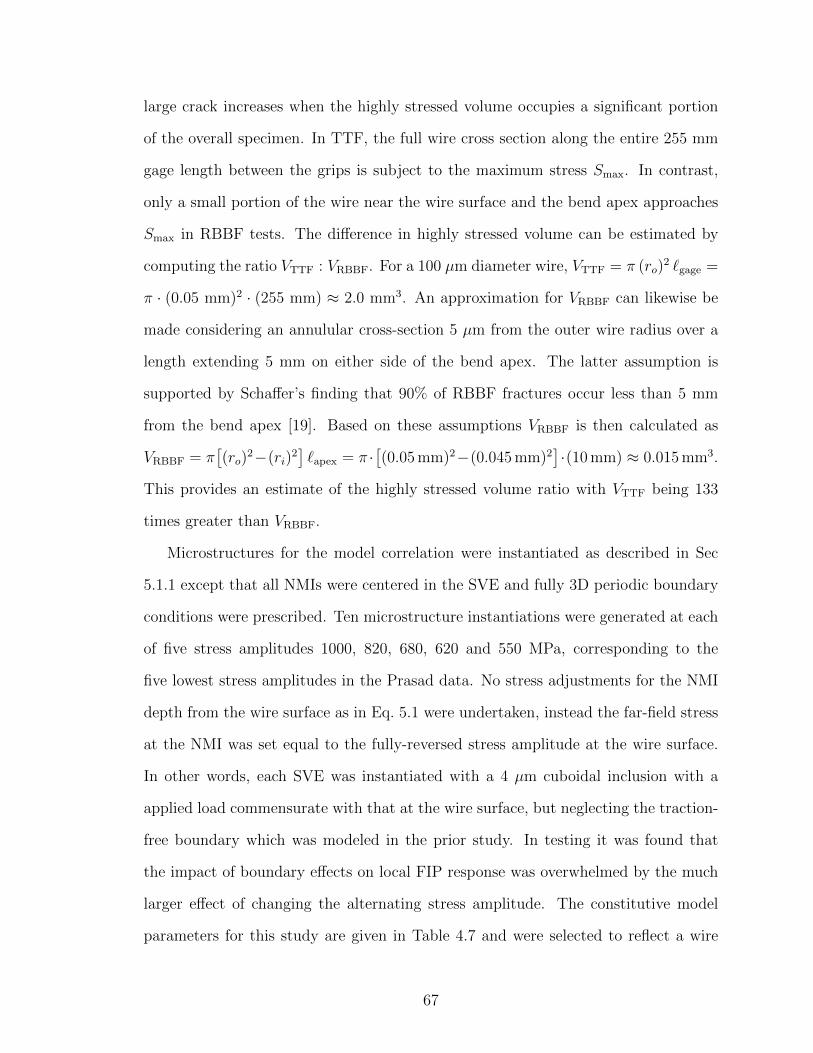
large crack increases when the highly stressed volume occupies a significant portion
of the overall specimen. In TTF, the full wire cross section along the entire 255 mm
gage length between the grips is subject to the maximum stress Smax. In contrast,
only a small portion of the wire near the wire surface and the bend apex approaches
Smax in RBBF tests. The difference in highly stressed volume can be estimated by
computing the ratio VTTF : VRBBF. For a 100 µm diameter wire, VTTF = π (ro)2 `gage =
π · (0.05 mm)2 · (255 mm) ≈ 2.0 mm3. An approximation for VRBBF can likewise be
made considering an annulular cross-section 5 µm from the outer wire radius over a
length extending 5 mm on either side of the bend apex. The latter assumption is
supported by Schaffer’s finding that 90% of RBBF fractures occur less than 5 mm
from the bend apex [19]. Based on these assumptions VRBBF is then calculated as
VRBBF = π[(ro)
2−(ri)2]`apex = π ·
[(0.05 mm)2−(0.045 mm)2
]·(10 mm) ≈ 0.015 mm3.
This provides an estimate of the highly stressed volume ratio with VTTF being 133
times greater than VRBBF.
Microstructures for the model correlation were instantiated as described in Sec
5.1.1 except that all NMIs were centered in the SVE and fully 3D periodic boundary
conditions were prescribed. Ten microstructure instantiations were generated at each
of five stress amplitudes 1000, 820, 680, 620 and 550 MPa, corresponding to the
five lowest stress amplitudes in the Prasad data. No stress adjustments for the NMI
depth from the wire surface as in Eq. 5.1 were undertaken, instead the far-field stress
at the NMI was set equal to the fully-reversed stress amplitude at the wire surface.
In other words, each SVE was instantiated with a 4 µm cuboidal inclusion with a
applied load commensurate with that at the wire surface, but neglecting the traction-
free boundary which was modeled in the prior study. In testing it was found that
the impact of boundary effects on local FIP response was overwhelmed by the much
larger effect of changing the alternating stress amplitude. The constitutive model
parameters for this study are given in Table 4.7 and were selected to reflect a wire
67
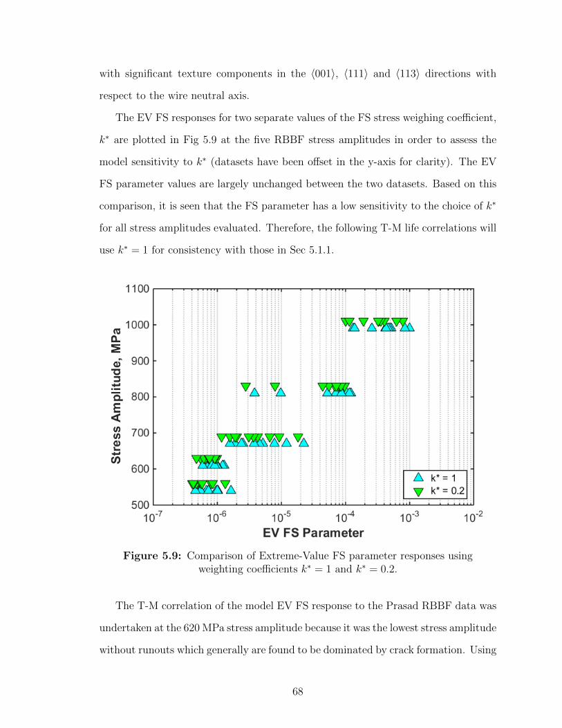
with significant texture components in the 〈001〉, 〈111〉 and 〈113〉 directions with
respect to the wire neutral axis.
The EV FS responses for two separate values of the FS stress weighing coefficient,
k∗ are plotted in Fig 5.9 at the five RBBF stress amplitudes in order to assess the
model sensitivity to k∗ (datasets have been offset in the y-axis for clarity). The EV
FS parameter values are largely unchanged between the two datasets. Based on this
comparison, it is seen that the FS parameter has a low sensitivity to the choice of k∗
for all stress amplitudes evaluated. Therefore, the following T-M life correlations will
use k∗ = 1 for consistency with those in Sec 5.1.1.
Figure 5.9: Comparison of Extreme-Value FS parameter responses usingweighting coefficients k∗ = 1 and k∗ = 0.2.
The T-M correlation of the model EV FS response to the Prasad RBBF data was
undertaken at the 620 MPa stress amplitude because it was the lowest stress amplitude
without runouts which generally are found to be dominated by crack formation. Using
68
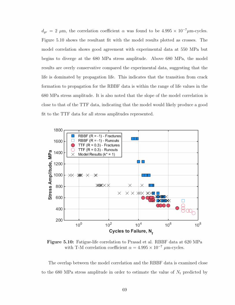
dgr = 2 µm, the correlation coefficient α was found to be 4.995 × 10⁻⁷µm-cycles.
Figure 5.10 shows the resultant fit with the model results plotted as crosses. The
model correlation shows good agreement with experimental data at 550 MPa but
begins to diverge at the 680 MPa stress amplitude. Above 680 MPa, the model
results are overly conservative compared the experimental data, suggesting that the
life is dominated by propagation life. This indicates that the transition from crack
formation to propagation for the RBBF data is within the range of life values in the
680 MPa stress amplitude. It is also noted that the slope of the model correlation is
close to that of the TTF data, indicating that the model would likely produce a good
fit to the TTF data for all stress amplitudes represented.
Figure 5.10: Fatigue-life correlation to Prasad et al. RBBF data at 620 MPawith T-M correlation coefficient α = 4.995× 10⁻⁷ µm-cycles.
The overlap between the model correlation and the RBBF data is examined close
to the 680 MPa stress amplitude in order to estimate the value of Nt predicted by
69
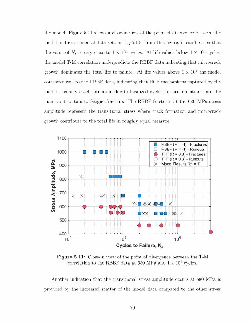
the model. Figure 5.11 shows a close-in view of the point of divergence between the
model and experimental data sets in Fig 5.10. From this figure, it can be seen that
the value of Nt is very close to 1 × 10⁵ cycles. At life values below 1 × 10⁵ cycles,
the model T-M correlation underpredicts the RBBF data indicating that microcrack
growth dominates the total life to failure. At life values above 1 × 10⁵ the model
correlates well to the RBBF data, indicating that HCF mechanisms captured by the
model - namely crack formation due to localized cyclic slip accumulation - are the
main contributors to fatigue fracture. The RBBF fractures at the 680 MPa stress
amplitude represent the transitional stress where crack formation and microcrack
growth contribute to the total life in roughly equal measure.
Figure 5.11: Close-in view of the point of divergence between the T-Mcorrelation to the RBBF data at 680 MPa and 1× 10⁵ cycles.
Another indication that the transitional stress amplitude occurs at 680 MPa is
provided by the increased scatter of the model data compared to the other stress
70
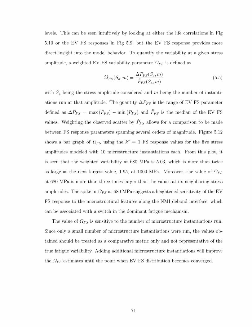
levels. This can be seen intuitively by looking at either the life correlations in Fig
5.10 or the EV FS responses in Fig 5.9, but the EV FS response provides more
direct insight into the model behavior. To quantify the variability at a given stress
amplitude, a weighted EV FS variability parameter ΩFS is defined as
ΩFS(Sa,m) =∆PFS(Sa,m)
PFS(Sa,m)(5.5)
with Sa being the stress amplitude considered and m being the number of instanti-
ations run at that amplitude. The quantity ∆PFS is the range of EV FS parameter
defined as ∆PFS = max (PFS) − min (PFS) and PFS is the median of the EV FS
values. Weighting the observed scatter by PFS allows for a comparison to be made
between FS response parameters spanning several orders of magnitude. Figure 5.12
shows a bar graph of ΩFS using the k∗ = 1 FS response values for the five stress
amplitudes modeled with 10 microstructure instantiations each. From this plot, it
is seen that the weighted variability at 680 MPa is 5.03, which is more than twice
as large as the next largest value, 1.95, at 1000 MPa. Moreover, the value of ΩFS
at 680 MPa is more than three times larger than the values at its neighboring stress
amplitudes. The spike in ΩFS at 680 MPa suggests a heightened sensitivity of the EV
FS response to the microstructural features along the NMI debond interface, which
can be associated with a switch in the dominant fatigue mechanism.
The value of ΩFS is sensitive to the number of microstructure instantiations run.
Since only a small number of microstructure instantiations were run, the values ob-
tained should be treated as a comparative metric only and not representative of the
true fatigue variability. Adding additional microstructure instantiations will improve
the ΩFS estimates until the point when EV FS distribution becomes converged.
71
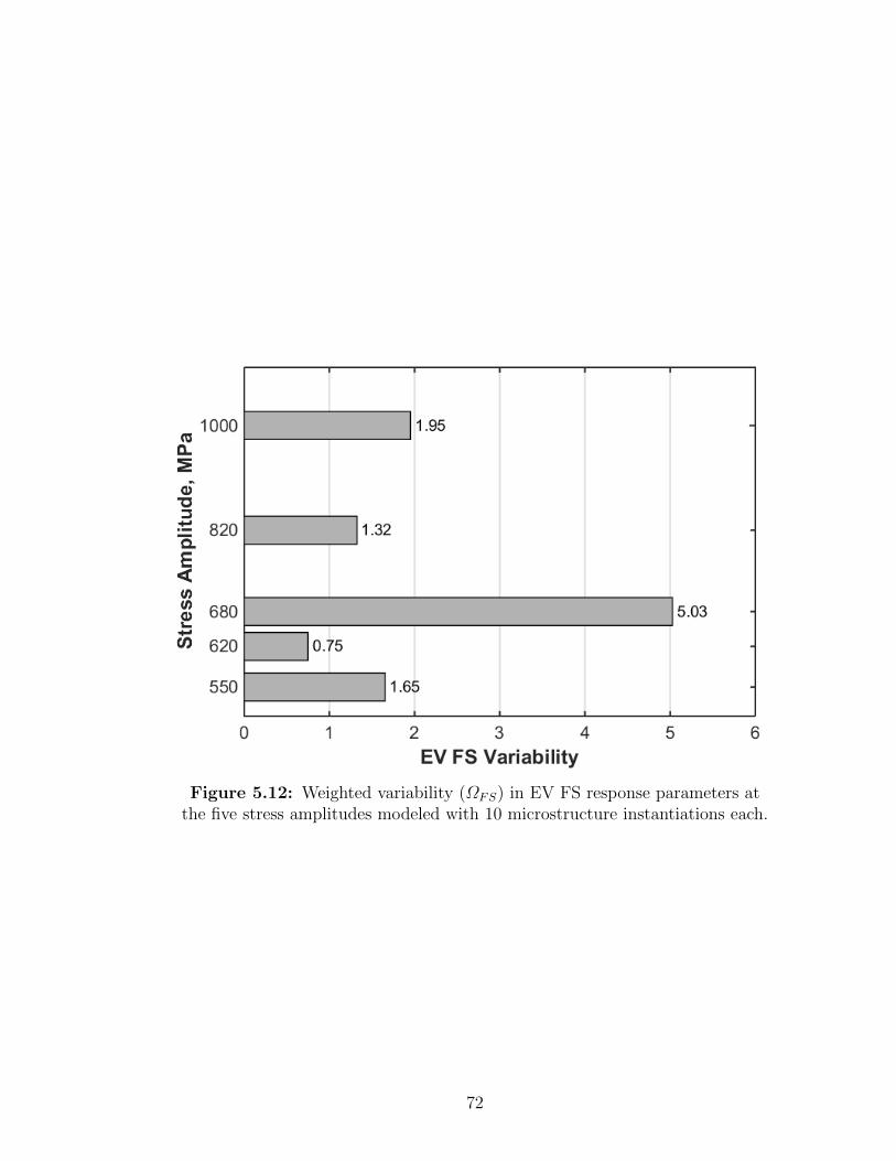
Figure 5.12: Weighted variability (ΩFS) in EV FS response parameters atthe five stress amplitudes modeled with 10 microstructure instantiations each.
72

CHAPTER VI
CONCLUSIONS
A physically-based, rate-dependent crystal viscoplasticity constitutive model was de-
veloped building off the work of Shenoy [21] which represents the isothermal mechan-
ical behavior of single-phase fcc MP35N alloy material. Deformation processes at and
above the grain scale are modeled, including accumulation of plastic shear strain on
preferred slip systems and isotropic and kinematic hardening. The model also ac-
counts for hardening due to nano-scale twinning through a homogenization approach.
The model parameters were fit to experimental monotonic tensile loading curves and
cyclic tension-tension experiments promoting strain ratcheting and adequately model
the material behavior under monotonic and cyclic loading conditions.
A microstructure generation tool was developed to construct statistical volume
elements (SVEs) reflecting the fine-grained microstructure and fiber texture charac-
teristic of MP35N fine wire. This includes (1) an algorithm for seeding ellipsoidal
grains by sampling from a lognormal distribution matched to experimentally charac-
terized grain size distributions for MP35N wire, (2) the ability to impose non-random
grain texture distributions mimicking MP35N EBSD scans with fiber texture, (3)
a scheme for placing hard non-metallic inclusions (NMIs) into SVEs with control
over the NMI-matrix interface, and (4) a meshing algorithm to maximize resolution
of stress gradients near the NMI while maintaining computational efficiency to run
fatigue loading cycles within the ABAQUS finite-element solver.
A modified Tanaka-Mura incubation life correlation methodology was employed to
73

correlate the volume-averaged extreme-value Fatemi-Socie parameter near the NMI-
matrix interface with the HCF behavior of MP35N wire. The model correctly pre-
dicted the fatigue life behavior resulting from variation of NMI proximity to the wire
surface in full-Ti MP35N wires run under rotating beam bending fatigue (RBBF)
loading at 620 MPa. A significant reduction in fatigue potency was found when
NMIs became fully embedded (xsurf ≥ dNMI) in the wire, consistent with experi-
mental results. The same correlation scheme was also used to identify the transition
life Nt between crack incubation and microcrack growth dominated fatigue regimes
for low-Ti MP35N wire loaded in RBBF. The transition life was estimated to be
Nt = 1 × 10⁵ cycles based on the point of divergence between the model correlation
at 680 MPa and the S-N curve. At life values above Nt, the model fit showed good
overlap with the experimental data, but a life values below Nt the model fit was overly
conservative for RBBF, indicating that crack formation was no longer the dominant
fatigue mechanism. It is anticipated that the model would correlate well to the TTF
dataset due to the reduced amount of microcrack growth present in force-controlled
modes of fatigue.
74

CHAPTER VII
RECOMMENDATIONS FOR FURTHER STUDY
The results presented in this work are by no means an exhaustive exploration of all
applications and uses for the model. A number of recommendations for continued
study are put forth here which go beyond the scope of the current work.
7.1 Ranking of Microstructure Attributes by Fatigue Po-tency
A ranking scheme to categorize and rank the microstructure attributes by fatigue
potency could be employed to identify the microstructure configurations with the
highest impact on fatigue life. The impact of NMI proximity to the free surface has
already been considered in Ch. 5. Additional microstructure attributes which may be
of interest include the morphology, size and composition of the NMI, the configuration
of the NMI-matrix interface, and the presence of other defect types such as surface
scratches or sub-surface voids. These attributes can be compared and ranked through
the use of extreme-value marked correlation functions as employed by Przybyla [16].
The use of these functions allows different microstructure attributes to be ranked
by their impact on fatigue and can also assess the impact of interactions between
microstructure attributes.
7.1.1 NMI Morphology
It is of interest to study the impact of inclusion morphology on fatigue crack initia-
tion potency. In addition to the cuboidal shapes considered in this work, spherical,
elliptical and octahedral inclusion geometries may also be considered. In the cases of
octahedral or cuboidal inclusions, the presence of sharp corners may add stress risers
75

in addition to those which are already present due to the strain mismatch between
the matrix and the embedded NMI particle. In these cases, the orientation of the
NMI with respect to the principle loading axis is an additional consideration that
should not be neglected.
7.1.2 NMI-matrix Interface
The condition of the NMI-matrix interface should also be considered in assessing
the microstructure for fatigue initiation potency. Interface delamination between the
matrix and the NMI particle can cause a heightened stress state and serve as an
embryonic crack from which the crack can propagate into the matrix. The extent of
the NMI-matrix delamination along with its orientation in relation to cyclic loading
axis dictates its potency to drive the generation and growth of fatigue cracks. Some
common interface conditions observed include fully bonded, partially debonded, fully
debonded and cracked NMIs.
While the present work has investigated partially debonded NMIs due to a pre-
liminary assessment that this condition represented a high driver for crack initiation,
the relative potency of these NMI-matrix interface conditions has not been rigorously
established. The microstructure generation tool has options to select from several
NMI-matrix interface scenarios on a cuboidal inclusion, and could be adapted to
mesh others. Figure 4.2 shows some of the NMI-matrix debonding scenarios available
in the microstructure generation tool.
7.1.3 Alternative Crack Initiation Sites
In the prior discussion, it has been assumed that fatigue cracks initiate at NMIs asso-
ciated with the generation of local stress risers and elastic mismatch strains. However,
other types of crack initiation sites are possible and are sometimes observed in fine
MP35N wires. Other defects which have been observed in MP35N wires are sur-
face scratches from the die drawing process and large grain-mediated crack initiation.
76

Surface scratches act in a similar manner to notches. Fatigue crack initiation due to
notches was explored by Musinski [11]. The role of large-grain mediated crack forma-
tion in HCF can also be addressed using the current methodology, provided data on
large-grain distributions in the drawn wire is available.
77

REFERENCES
[1] Asgari, S., El-Danaf, E., Shaji, E., R., K. S., and Doherty, R. D.,“The secondary hardening phenomenon in strain-hardened MP35N alloy,” ActaMetallurgica, vol. 46, no. 16, pp. 5795–5806, 1998.
[2] ASTM F562-13, “Standard specification for wrought 35cobalt-35nickel-20chromium-10molybdenum alloy for surgical implant applications (UNSR30035),” 2013.
[3] Castelluccio, G. M. and McDowell, D. L., “Assesment of small fatiguecrack growth driving forces in single crystals with and without slip bands,” In-ternational Journal of Fracture, vol. 176, pp. 49–64, 2012.
[4] Dassault Systemes, “Abaqus v6.14-1,” 2014. Providence, RI, USA.
[5] El-Danaf, E., Kalidindi, S. R., and Doherty, R. D., “Influence of de-formation path on the strain hardening behavior and microstructure evolutionin low SFE FCC metals,” International Journal of Plasticity, vol. 17, pp. 1245–1265, 2001.
[6] Fatemi, A. and Socie, D., “A critical plane approach to multiaxial fatiguedamage including out-of-phase loading,” Fatigue and Fracture of EngineeringMaterials and Structures, vol. 11, no. 3, pp. 149–165, 1988.
[7] Li, B. and Steigauf, T., “Crystallography texture and mechanical propertiesof MP35N wire,” in Materials Processes for Medical Devices Conference, ASM,September 2007.
[8] MathWorks, Inc, “Matlab, R2014b,” 2014. Natick, MA, USA.
[9] Musinski, W., Modeling the Effects of Shot-Peened Residual Stresses and In-clusions on Microstructure-sensitive Fatigue of Ni-Base Superalloy Components.PhD thesis, Georgia Institute of Technology, August 2014.
[10] Musinski, W. D., “Novel methods for microstructure-sensitive probabilisticfatigue notch factor,” Master’s thesis, Georgia Institute of Technology, August2010.
[11] Musinski, W. D. and McDowell, D. L., “Microstructure-sensitive proba-bilistic modeling of HCF crack initiation and early crack growth in Ni-base su-peralloy IN100 notched components,” International Journal of Fatigue, vol. 37,pp. 41–53, 2012.
78

[12] Office of Science and Technology Policy, “Materials genome initia-tive for global competitiveness,” white paper, National Science and TechnologyCouncil, June 2011.
[13] Ornberg, A., Pan, J., Herstedt, M., and Leygraf, C., “Corrosion resis-tance, chemical passivation, and metal release of 35N LT and MP35N for biomed-ical material application,” Journal of the Electrochemical Society, vol. 154, no. 9,pp. C546–C551, 2007.
[14] Prasad, M., Reiterer, M., and Kumar, K., “Microstructure and mechanicalbehavior of an as-drawn MP35N alloy wire,” Material Science & Engineering A,vol. 610, pp. 326–337, 2014.
[15] Przybyla, C. P., Microstructure-sensitive Extreme Value Probabilities of Fa-tigue in Advanced Engineering Alloys. PhD thesis, Georgia Institute of Technol-ogy, 2010.
[16] Przybyla, C. P. and McDowell, D. L., “Simulated microstructure-sensitiveextreme value probabilities for high cycle fatigue of duplex Ti-6Al-4V,” Interna-tional Journal of Plasticity, 2011.
[17] Raghavan, M., Berkowitz, B. J., and Kane, R. D., “A transmission elec-tron microscopic investigation of phase transformations in MP35N,” Metallur-gical and Materials Transactions A: Physical Metallurgy and Materials Science,vol. 11A, pp. 203–207, 1980.
[18] Salajegheh, N. and McDowell, D. L., “Microstructure-sensitive weightedprobability approach for modeling surface to bulk transition of high cycle fa-tigue failures dominated by primary inclusions,” International Journal of Fa-tigue, vol. 59, pp. 188–199, 2014.
[19] Schaffer, J. E., “A hierarchical initiation mechanism approach to modelingfatigue life variability in 35Co-35Ni-20Cr-10Mo alloy medical grade fine wire,”Master’s thesis, Purdue University, 2007.
[20] Schaffer, J. E., “An examination of fatigue initiation mechanism in thin35Co-35Ni-20Cr-10Mo medical grade wires,” ASTM International, vol. 5, pp. 1–10, July 2008.
[21] Shenoy, M., Tjiptowidjojo, Y., and McDowell, D. M., “Microstructure-sensitive modeling of polycrystalline IN 100,” International Journal of Plasticity,vol. 24, pp. 1694–1730, 2008.
[22] Shenoy, M., Zhang, J., and McDowell, D. L., “Estimating fatigue sen-sitivity to polycrystalline ni-base superalloy microstructures using a computa-tional approach,” Fatigue and Fracture of Engineering Materials and Structures,vol. 30, pp. 889–904, 2007.
79

[23] Sorensen, D., Li, B., Gerberich, W., and Mkyoyan, K., “Investigationof secondary hardening in Co-35Ni-20Cr-10Mo alloy using analytical scanningtransmission microscopy,” Acta Materialia, 2013.
[24] Suresh, S., Fatigue of Materials. Cambridge University Press, second ed., 1998.
[25] Tanaka, K. and Mura, T., “A dislocation model for fatigue crack initiation,”Journal of Applied Mechanics, vol. 48, pp. 97–103, 1981.
[26] Wang, Y., Wang, J. J., Zhang, H., Manga, V. R., Shang, S. L., Chen,L.-Q., and Liu, Z.-K., “A first-principles approach to finite temperature elasticconstants,” Journal of Physics: Condensed Matter, vol. 22, pp. 225404–225412,2010.
80