


1
METHODOLOGIES AND PROGRAMMING DEVELOPMENT OF APPLICATIONS ON MODELING, IDENTIFICATION AND SIMULATION
EPN JOURNAL, VOL. 33, NO. 1, MAY 2013
1. INTRODUCTION
Modeling, simulation and identification of prototypes are a
fundamental part of controllers design, obtained by
mathematical modeling expressed as state variables, transfer
functions and differential equations. From control system
focusing, the goal of modeling is to find a system’s analytic
model which allows designing the right controller to close the
system’s loop to implement a correct dynamic system’s
operation, saving resources and let system quality get better.
This paper introduces different methods of modeling that
makes it easier to obtain its state variables, transfer function
and differential equations. These methods [1] use
interconnection restrictions to flux and effort, theory of
electrical nets by applying node matrix equations and
interconnection restrictions based on Lagrangian calculation.
Simulation is useful due to mathematical problem solutions
in systems which analytic solution is unknown or in
mathematical processes where the solution is complex when
trying to calculate the analytic solution without any
computational device. The simulation allows finding
solutions to problems where experimentation is expensive
and allows the investigation of possible control strategies,
while providing a more realistic replica of a system.
Presenting a modeling and identification software allows
obtaining the system answers according to the input
specifications. Identification is acquired from experimental
data by applying several iterations applied to the approximate
equation of the line with nearby points and neglecting the
experimental points coming out of the expected range of
measurements.
Methodologies and Programming Development of Applications on Modeling,
Identification and Simulation
Cabezas L.*, Rosales A.*, Burbano P.*
*Escuela Politécnica Nacional, Departamento de Automatización y Control Industrial, Quito, Ecuador
(e-mail:[email protected]; [email protected]; [email protected])
Resumen: La modelación, simulación e identificación de prototipos permiten realizar
predicciones acertadas del comportamiento de los sistemas, además de hallar las expresiones
matemáticas tales como funciones de transferencia, ecuaciones diferenciales y variables de
estado necesarias para la implementación de controladores, sin necesidad de la
implementación de los prototipos reales, lo que permite simular en un entorno similar las
perturbaciones o simplemente observar su respuesta en condiciones normales. Este trabajo
presenta la modelación de varios sistemas, utilizando diversos métodos sean éstos directos, de
redes o variacional, además del desarrollo de metodologías enfocadas al desarrollo de casos
de estudio, a través de los cuales se implementa cinemática inversa, transformaciones
homogéneas, métodos de Newton-Euler, Euler-Lagrange y otros que facilitan la simulación
de sistemas a través de Matlab.
Palabras clave: Robótica, Modelación, Simulación, Identificación, Procesos.
Abstract: Modeling, simulation and identification of prototypes allow people to make right
predictions about the behavior of systems also finding mathematical expressions such as
transfer functions, differential equations and state variables needed to control implementation
without being necessary to implement real prototypes which allow to simulate in a similar
environment as the one with perturbation or simply observe the dynamical response in normal
conditions. This paper is focused on modeling various systems, using diverse modeling
methods as direct, net method or variational, also the development of methodologies dedicated
on study cases developing through which is implemented inverted kinematics, homogenous
transformations, Newton-Euler method, Euler-Lagrange method and some other methods that
makes it simple to run system simulations on Matlab
Keywords: Modeling, Identification, Simulation, Robotics, Process.

2
METHODOLOGIES AND PROGRAMMING DEVELOPMENT OF APPLICATIONS ON MODELING, IDENTIFICATION AND SIMULATION
EPN JOURNAL, VOL. 33, NO. 1, MAY 2013
2. DEVELOPMENT OF METHODOLOGIES FOR
MODELING AND IDENTIFICATION
A model is a simplified representation of a system which
answers to questions about the specified system are obtained
without using experimentation.
For identification, reaction curve is used for obtaining steady-
state value of the system, this value is obtained by
performing a measurement of the process and make a curve
with the input and output values over time.
2.1 Direct Method
The procedure of modeling by using the direct method lets
select the variables involved in a system, whether it is
physical, electrical, mechanical, fluid, etc. The direct method
allows the visualization of the direction of the forces
applying physics by Newton's laws (Figure1).
Figure 1. Mechanic System
The system of Figure 1 is used for analysis by the direct
method, for which it has several steps to obtain its differential
equations and state variables.
1. Write a free body diagram, considering forces that act
over it.
2. Applying Newton's second law, which intervenes the
sum of the forces acting on the body, in the system acts
four forces and are represented according to the direction
of the mass 1.
1kf = force produced by the spring
1Bf = force produced by the buffer
1mf = reaction effort produced by the action of force
f= force produced by action
3. Write the sum of forces accordingly to the body free
diagram.
=
==
===
=++
=
•
•••
∑
111
11111
1111111
111
0
ykf
yBvBf
ymvmamf
ffff
f
k
B
m
kBm
fykyBym =++•••
11111 (1)
4. Write the state variables according to the input and
output applied to the system, in this case the system
input is the action force f and output variables are the
displacement and speed.
=
2
1
1
1
x
x
v
y
1yy
fu
=
=
5. To describe each of the variables to obtain the matrices
corresponding to the state variables.
1v = mass speed 1 and equivalent to the first
derivative of displacement and equal to
dtdy /1
11 xy = = movement performed by the mass1
121
•
== xxv = mass 1 speed
6. Replace the state variables in equation 1 for the state
matrix.
um
xm
Bx
m
kx
uxkxBxm
fykyBym
1
2
1
11
1
12
112121
111111
1+−−=
=++
=++
•
•
•••
Figure 2. Free body diagram

3
METHODOLOGIES AND PROGRAMMING DEVELOPMENT OF APPLICATIONS ON MODELING, IDENTIFICATION AND SIMULATION
EPN JOURNAL, VOL. 33, NO. 1, MAY 2013
( ) 001
1010
2
1
12
1
1
1
1
1
2
1
=
=
+
−−=
•
•
Dx
xy
u
mx
x
m
B
m
k
x
x
(2)
Equation 2 represents the matrix of variable states resulting
A, B, C, D.
−−=
1
1
1
1
10
m
B
m
kA = State Matrix
=
1
10
m
B = Input Matrix
( )01=C = Output matrix
0=D =Zero matrix or direct transition matrix.
2.2 Nets method
The method of generalized nets or nets is formed by the
interconnection of elements and widespread sources that
represent different kinds of physical elements and variables
involved in it allows obtaining quantities that describe the
dynamic behavior of the same system. An electrical
equivalent from a mechanical system benchmarks required
for processing and proper connection. It is necessary to
identify whether the variables are transvariables or per
variables.
1) Transvariables: those variables that require two
points to be measured and are obtained through
resistors, inductors or capacitors.
2) Pervariables: those variables that are propagated by
the elements and for which measurement is required
only one point.
Table 1 is analyzed considering the mechanical, fluid and
electrical equivalent that facilitates the resolution of problems
that arise around the modeling of systems.
Table 1. Mechanical and electrical analogies
The mechanical system shown in Figure 2 is transformed
toan electrical system through respectively equivalents
according to Table 1.Observing the elements of the system
and performing a comparison table to facilitate the
transformation of electrical into mechanical elements, in this
case the system comprises a damper and a spring supported
mass through these elements to a reference system which the
wall and the floor. which is subject of the aforementioned
elements.
The characteristics of the processed electrical mechanical
elements are deduced from this comparison:
ifluxforcef
velocityvefforte
===
===
positionyOutput
ufnput
==
==I
.
1
1
i
i
a i
div L
dt
div dt L dt
dt
e v dt x Li Lf
f x kxL
Lk
=
=
= = = =
= =
=
∫ ∫
∫
Force produced by the buffer vBfB .= goes like B/1
∴==flux
effort
Bf
v 1 It is equivalent to RI
V=
Bf
vR
1==
Construction begins with the equivalent circuit for the main
mass of the system as it is transformed into a grounded
4
METHODOLOGIES AND PROGRAMMING DEVELOPMENT OF APPLICATIONS ON MODELING, IDENTIFICATION AND SIMULATION
EPN JOURNAL, VOL. 33, NO. 1, MAY 2013
capacitor mentioned, we consider each point mass or speed
for the circuit node, in this case comes only a node that is
connects the elements in the system. It is recommended that
in order of appearance in the circuit elements with reference
to the capacitor referred to ground, the coil must be placed to
the left of it and the resistor on the right side of the capacitor.
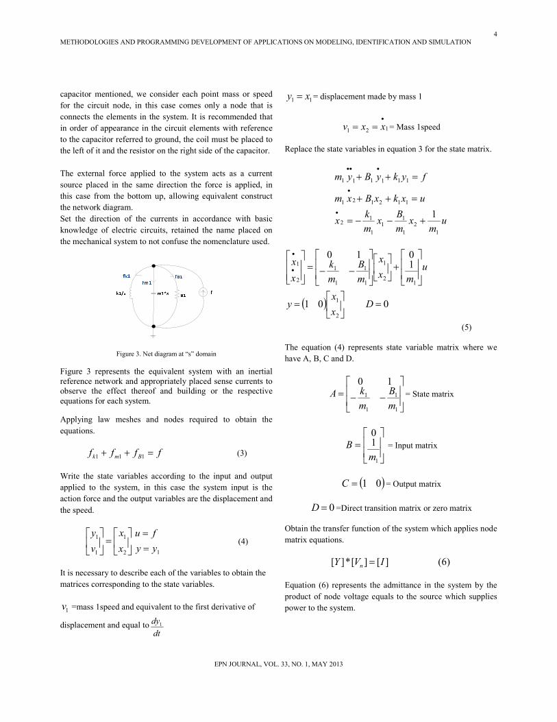
The external force applied to the system acts as a current
source placed in the same direction the force is applied, in
this case from the bottom up, allowing equivalent construct
the network diagram.
Set the direction of the currents in accordance with basic
knowledge of electric circuits, retained the name placed on
the mechanical system to not confuse the nomenclature used.
Figure 3. Net diagram at “s” domain
Figure 3 represents the equivalent system with an inertial
reference network and appropriately placed sense currents to
observe the effect thereof and building or the respective
equations for each system.
Applying law meshes and nodes required to obtain the
equations.
ffff Bmk =++ 111 (3)
Write the state variables according to the input and output
applied to the system, in this case the system input is the
action force and the output variables are the displacement and
the speed.
=
2
1
1
1
x
x
v
y
1yy
fu
=
= (4)
It is necessary to describe each of the variables to obtain the
matrices corresponding to the state variables.
1v =mass 1speed and equivalent to the first derivative of
displacement and equal todt
dy1
11 xy = = displacement made by mass 1
121
•
== xxv = Mass 1speed
Replace the state variables in equation 3 for the state matrix.
um
xm
Bx
m
kx
uxkxBxm
fykyBym
1
2
1
11
1
12
112121
111111
1+−−=
=++
=++
•
•
•••
( ) 001
1010
2
1
12
1
1
1
1
1
2
1
=
=
+
−−=
•
•
Dx
xy
u
mx
x
m
B
m
k
x
x
(5)
The equation (4) represents state variable matrix where we
have A, B, C and D.
−−=
1
1
1
1
10
m
B
m
kA = State matrix
=
1
10
m
B = Input matrix
( )01=C = Output matrix
0=D =Direct transition matrix or zero matrix
Obtain the transfer function of the system which applies node
matrix equations.
)6(][][*][ IVY n =
Equation (6) represents the admittance in the system by the
product of node voltage equals to the source which supplies
power to the system.

5
METHODOLOGIES AND PROGRAMMING DEVELOPMENT OF APPLICATIONS ON MODELING, IDENTIFICATION AND SIMULATION
EPN JOURNAL, VOL. 33, NO. 1, MAY 2013
++==
==
++
=
111
1
1111
1
)(
)(
][][*][
Bsms
kINPUT
OUTPUT
sF
sV
fIVBsms
k
IVY n
)()(
)(1
11
2
1
1 sGksBsm
s
sF
sV=
++=
(7)
Correctly applying the equivalent net for mechanical systems
and other fluid is readily to write differential equations, state
variables and transfer function posed systems without
considering free body diagrams, physical laws and direction
of forces applied.
2.3Variational method
The mathematical models of physical systems (mechanical,
electrical, etc.) can be derived from energy considerations
without applying Newton's laws or Kirchhoff’s laws. The
mechanical equations of motion feature need to be derived,
by using for the potential and kinetic energy thereof.
In deriving the equations of motion for a complicated
mechanical system, it should be done using two different
methods (one based on Newton's second law and the other by
considering energy acting on the system). The Lagrange
method is a successful appeal to derive equations for this
system class.
To derive the Lagrange equations of motion is necessary to
define the generalized coordinates and the Lagrangian, to
establish the principle of Hamilton[1]. Simplified model of a
manipulator without considering the moment of inertia of the
masses of each end of the robotic arm is considered. It
disregards the moments of inertia for an idealized model of
the system and easily to deduce the mathematical model.
Figure 4. Simplified manipulator
To apply the variational method is necessary to consider the
initial conditions:
• Rotation of the masses schedule.
• Set point mass 2, the floor is subject to where the first
link, the reference is moved to the second link.
1. Performing speed diagram to determine the net rate at
which the mass 2 moves, it is necessary to move in the
same diagram references to relate vectors and
complementary and supplementary angles.
α
Figure 5. Relative speed diagram.
2. Performing the sum of the angles corresponding to the
mass such that two have a supplementary angle, the sum
is equals to 180 °, and thus obtain the equivalent angle
α .
2
2 1809090
θα
θα
=
=−++

6
METHODOLOGIES AND PROGRAMMING DEVELOPMENT OF APPLICATIONS ON MODELING, IDENTIFICATION AND SIMULATION
EPN JOURNAL, VOL. 33, NO. 1, MAY 2013
3. Applying cosine law to determine once found the
equivalent in terms of known angles relative speed of the
second link is a function of the angle 1 and speed 2 2θ :
= + − 2 cos180 − = + + 2 cos (8)
4. Selecting generalized coordinates, these coordinates are
independent and are necessary to describe the motion of
the system, the number of variables depends on the
degrees of freedom possessed by the system. In this case,
are two coordinates: , .
5. Selecting variational coordinates, these are the variables
that place restrictions and permissible variations must be
allowed throughout the operation of the: , .
6. Calculate the Lagrangian, co-energy and co-contained, it
is necessary to obtain the kinetic and potential energy of
the system in a single expression that allows to apply the
Euler-Lagrange equation based on terms of work and
energy, all shares not generate a job are not considered
for the system in this method.
= ∗ − ,. This method derives the equations of motion for a
complicated mechanical system. It should be done using two
variables.
*U = co-energy directly related to the kinetic energy of the
system components, these are capacitive elements electrically
and mechanically mass. Kinetic energy of the entire system
thus comprises the sum of the partial kinetic energies of each
link with proper mass.
= ∗ = 12
∗ = + (9)
The expression (9) links the angular speed with which the
linear speed:
=v linear speed link
==•
θw angular speed
=θ angular displacement
=l length of each link
= ! (10)
7. Replacing the expression (10) in (9) to obtain an
expression in terms of the system parameters, they are:
nnn lm θ,, .
∗ = !" + #$!" % + $!" % +2!!" " cos & (10)
' = 12()* = 12+, = 0
- = ∗ − '; ' = 0
- = ∗ Non dissipative and inductive elements or G and L which are
zero and calculating Lagrangian depends only on the co-
energy stored in capacitive effect devices such as each link of
the robotic arm with two degrees of freedom because it has
masses own.
- = !" + #$!" % + $!" % +2!!" " cos & (11)
8. For each variational coordinate apply the Euler-Lagrange
equation, the Lagrangian L is subjected to referral for
each acting variable on the system.
For:
//0 1 2-2" 3 − 2-2 + 2*2" = 4
//0 1 2-2" 3 = //0 1 22" 512!" + 12 #$!" % + $!" %+ 2!!" " cos &63
7
METHODOLOGIES AND PROGRAMMING DEVELOPMENT OF APPLICATIONS ON MODELING, IDENTIFICATION AND SIMULATION
EPN JOURNAL, VOL. 33, NO. 1, MAY 2013
//0 1 2-2" 3 = 7!8 +!8 +!!8 cos −!!" sin = 4; +!8 + !!$8 <=> − " sin % = 4
(12)
For :
//0 1 2-2" 3 − 2-2 + 2*2" = 4
//0 1 2-2" 3 = //0 ?12! ∗ 2 ∗ " + 12 ∗ ∗ 2∗ !!"<=>@ 2-2 = −12 ∗ 2 ∗ !!"">AB
222121221212122
2
22 cos τθθθθθθθθ =+
−+
•••••••
senllmsenllmlm (13)
Equations (12) and (13) are the differential equations that
representing the system, and they are obtained by
differentiating the Lagrangian with respect of each variational
coordinate obtained from the sum of energies that act on the
system.
9. State variables Model given the parameters of the system
allows the nonlinear model of proposed system.
The equation sets the inverse dynamic model of a robot,
giving couples who must provide actuators for joint variables
follow a certain path =θ , where:
=)(θH inertia matrix
=•
),( θθc matrix centrifugal and Coriol is accelerations
=)(θg gravity matrix
=τ torque or twisting torque applied to each link
τθθθθθ =++•••
)(),(*)( gcH
=
+
+
•
•
••
••
2
1
2
1
2
1
2221
1211
2
1
2221
1211
ττ
θ
θ
θ
θg
g
cc
cc
hh
hh
(14)
Equation (14) represents a simplified general dynamic model
of a robot.
( )
0)(
0)(
),(
),(
),(
0),(
)(
cos)(
cos)(
)(
2
1
2121222
22212221221
221212
11
2
2222
221221
221212
2
12
2
1111
=
=
=
+−=
−=
=
=
=
=
+=
••
••
•
•
θ
θθθθθ
θθθθθ
θθθ
θθ
θ
θθ
θθθ
g
g
senllmc
senllmsenllmc
senllmc
c
lmh
llmh
llmh
lmlmh
3. DEVELOPMENT CASE STUDIES
The approach presented in the case studies covers areas of
robotics, process and other areas of interest in the “Escuela
Politécnica Nacional”, identification and robot modeling
approach facilitates control solutions also allows testing in
this model before implemented by simulation, generating
research and resource depletion when placing controllers,
actuators and other already known since the system behavior
is available.
3.1 ROBOTINO ®
To obtain the mathematical model of the omnidirectional
mobile robot Robotino is necessary to consider the three
degrees of mobility it possesses due to its three wheels.
Omnidirectional wheels, in addition to the basic movements
back and forth, allowed complicated movements: movements
in all directions, diagonally, laterally and even 360 °.

8
METHODOLOGIES AND PROGRAMMING DEVELOPMENT OF APPLICATIONS ON MODELING, IDENTIFICATION AND SIMULATION
EPN JOURNAL, VOL. 33, NO. 1, MAY 2013
Figure 6. Robotino Geometry for the kinematic model
Figure 6 shows a top view of the configuration of the mobile
robot, this identifies the mobile framework Xr, Yr situated
in the center of the vehicle. The fixed reference axis is the
XY, which travel speeds Vector:
T
w vvvv ][ 321= (15)
Unit vector:
( )( )ψψ
ψψ
+=⋅
+⋅=⋅
11
1111
cos
cos
r
r
XD
XDXD (16)
The speed of each wheel and the speed of the robot is
expressed by rotation of a unit vector in the direction Xr.
( ) ( )( ) ( )
( )( )
+
+=
+−+
++=
ψϕψϕ
ψϕψϕψϕψϕ
i
i
ii
ii
isensen
senv
cos
0
1
cos
cos (17)
To get the cosine term of robot movement is necessary to
rotate the wheel, and the sine is obtained by moving the
wheels laterally.
Equation (17) indicates the movement of the wheels and the
robot without considering the rotation angle which arises in
equation (18) as the rotation part in the cosine and the
tangential rotationΩ , according to movement of
omnidirectional wheels .2/90 πψ =°= [2]
( ) ( )( ) ( )( ) ( )
Ω
⋅
++−
++−
++−
=
=
•
•
ω
ω
ϕθϕθϕθϕθϕθϕθ
y
x
R
R
R
rv
v
v
rw
w
w
33
22
11
3
2
1
3
2
1
cossin
cossin
cossin11 (18)
The dynamic model of the mobile robot is obtained from the
Euler-Lagrange method. For which it is considered that the
center of mass G is at the origin of the reference axes mobile.
It follows the dynamic model of the system in the form:
τBQQCQD =
+
••••
(19)
+
+
+
=
2
2
2
2
2
300
02
30
002
3
r
IrRI
Mr
Ir
Mr
Ir
D
R
R
R
−
=•
•
•
000
00
00
2
3)(
2ϕ
ϕ
r
IrQC
(20)
+−+
+−+−
=
RRR
sen
sensen
rϕϕθϕθϕϕθϕθ
β )cos()cos(
cos)()(1
3.2 Helicopter Two Degrees of Freedom
A helicopter flies by a plane same principles, but in the case
of helicopters lift is achieved by rotating blades. These make
the lift possible. Its shape produces a force when the air
passes through them. The rotor blades are profiles designed
specifically for the flight characteristics. [3]
Figure 7. Helicopter Dynamics [4]
The chopper rotates over an angle Ψ Z and Y with respect to
an angle θ, so it considers the position of the center of mass
with respect to a fixed coordinate system [5].
We use homogeneous transformation matrixes
ψ,0zRot y θ,yRot

9
METHODOLOGIES AND PROGRAMMING DEVELOPMENT OF APPLICATIONS ON MODELING, IDENTIFICATION AND SIMULATION
EPN JOURNAL, VOL. 33, NO. 1, MAY 2013
−=
1000
100
0010
001
,,
2
0 10 h
l
RotRotT
mc
yz θψ
(21)
Is linearized around 0=θ
(22)
The values obtained for the state variables depends on the
value we assign to θ .
3.3 Identification in Time Tranche Pipeline
The section of pipeline that experimental data is discussed
was taken from SOTE (Sistema del Oleoducto Trans
Ecuatoriano) and the test was done in normal operating
conditions, a change is made passage of small amplitude set
point as an unscheduled stop produce consequences of time
and money [6].
Table 2. Variation of discharge pressure function of time
In the time domain response of anon-oscillatory system has
the form:
nt
n
tttekekekekAtC //
3
/
2
/
1 .......)( 321 −−−− +++++= τττ(23)
For a proper identification system requires multiple iterations
approaching a line of a first order type.
Where:
A= variation amplitude of the output signal,
iτ = system time constants.
n= order system,
ik =constant of proportionality.
If any dominant time constant is so large times the terms of
equation (23) having small time constants tend to zero, while
the end of the large time constant is still different from zero,
so that approaches:
0.......00)( 1/
1 +++++≈ − τtekAtC (24)
1/
1)(τt
ekAtC−+=
(25)
Fig. 8 Step function response, identifying the system
According to the actual model graphic representation of the
variation of the discharge pressure versus time, when excited
closed loop system a step function, and the model identified
according to the data transfer function allows to validate de
transfer function models after a few iterations.
10
METHODOLOGIES AND PROGRAMMING DEVELOPMENT OF APPLICATIONS ON MODELING, IDENTIFICATION AND SIMULATION
EPN JOURNAL, VOL. 33, NO. 1, MAY 2013
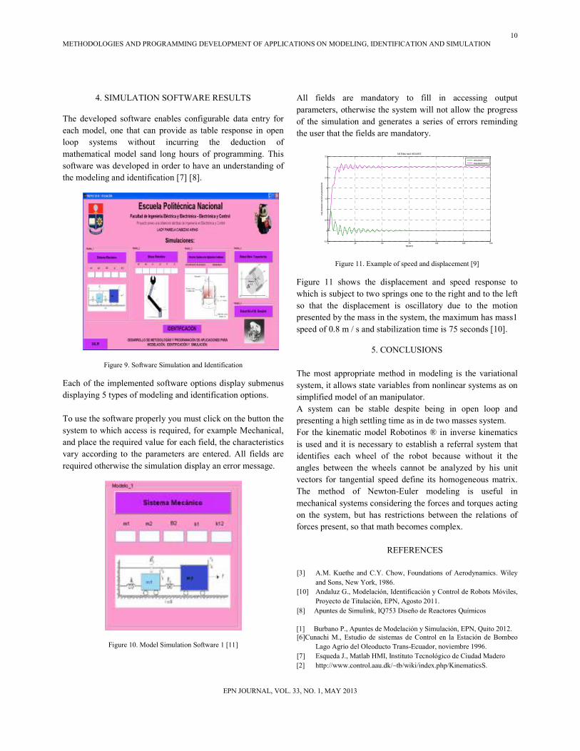
4. SIMULATION SOFTWARE RESULTS
The developed software enables configurable data entry for
each model, one that can provide as table response in open
loop systems without incurring the deduction of
mathematical model sand long hours of programming. This
software was developed in order to have an understanding of
the modeling and identification [7] [8].
Figure 9. Software Simulation and Identification
Each of the implemented software options display submenus
displaying 5 types of modeling and identification options.
To use the software properly you must click on the button the
system to which access is required, for example Mechanical,
and place the required value for each field, the characteristics
vary according to the parameters are entered. All fields are
required otherwise the simulation display an error message.
Figure 10. Model Simulation Software 1 [11]
All fields are mandatory to fill in accessing output
parameters, otherwise the system will not allow the progress
of the simulation and generates a series of errors reminding
the user that the fields are mandatory.
Figure 11. Example of speed and displacement [9]
Figure 11 shows the displacement and speed response to
which is subject to two springs one to the right and to the left
so that the displacement is oscillatory due to the motion
presented by the mass in the system, the maximum has mass1
speed of 0.8 m / s and stabilization time is 75 seconds [10].
5. CONCLUSIONS
The most appropriate method in modeling is the variational
system, it allows state variables from nonlinear systems as on
simplified model of an manipulator.
A system can be stable despite being in open loop and
presenting a high settling time as in de two masses system.
For the kinematic model Robotinos ® in inverse kinematics
is used and it is necessary to establish a referral system that
identifies each wheel of the robot because without it the
angles between the wheels cannot be analyzed by his unit
vectors for tangential speed define its homogeneous matrix.
The method of Newton-Euler modeling is useful in
mechanical systems considering the forces and torques acting
on the system, but has restrictions between the relations of
forces present, so that math becomes complex.
REFERENCES
[3] A.M. Kuethe and C.Y. Chow, Foundations of Aerodynamics. Wiley
and Sons, New York, 1986.
[10] Andaluz G., Modelación, Identificación y Control de Robots Móviles,
Proyecto de Titulación, EPN, Agosto 2011.
[8] Apuntes de Simulink, IQ753 Diseño de Reactores Químicos
[1] Burbano P., Apuntes de Modelación y Simulación, EPN, Quito 2012.
[6]Cunachi M., Estudio de sistemas de Control en la Estación de Bombeo
Lago Agrio del Oleoducto Trans-Ecuador, noviembre 1996.
[7] Esqueda J., Matlab HMI, Instituto Tecnológico de Ciudad Madero
[2] http://www.control.aau.dk/~tb/wiki/index.php/KinematicsS.
0 25 50 75 100 125 150-0.5
0
0.5
1
1.5
2
2.5
3
3.5
SISTEMA MAS RESORTE
TIEMPO
VELOCIDAD DESPLAZAMIENTO
velocidad1
desplazamiento1

11
METHODOLOGIES AND PROGRAMMING DEVELOPMENT OF APPLICATIONS ON MODELING, IDENTIFICATION AND SIMULATION
EPN JOURNAL, VOL. 33, NO. 1, MAY 2013
[9] Kuo Benjamín, “Sistemas de Control Automático” Séptima Edición
[5] M. Spong and M. Vidyasagar.Robot Dynamics and Control. John
Wiley & Sons, New York, 1 edition, 1989.
[11] Rosales A., Apuntes Control Computarizado, Escuela Politécnica
Nacional, Quito, 2012. [4] Vivas E., Control Helicóptero 2D usando métodos de control robusto


![SOFTWARE REQUIREMENTS ENGINEERING LECTURE # 2 AGILE METHODOLOGIES · 2013-04-11 · Extreme programming [21] Extreme Programming (XP) is a software development methodology which is](https://static.cupdf.com/doc/110x72/5f85cbd6ec5b2c0b897e977d/software-requirements-engineering-lecture-2-agile-methodologies-2013-04-11-extreme.jpg)


