ME 1020 Engineering Programming with MATLAB
Chapter 5 In-Class Assignment: 5.3, 5.6, 5.8, 5.12, 5.15, 5.18, 5.21, 5.26, 5.28, 5.30
Topic Covered:
xy Plotting Functions
Additional Commands and Plot Types
Interactive Plotting in MATLAB
Three-Dimensional Plots
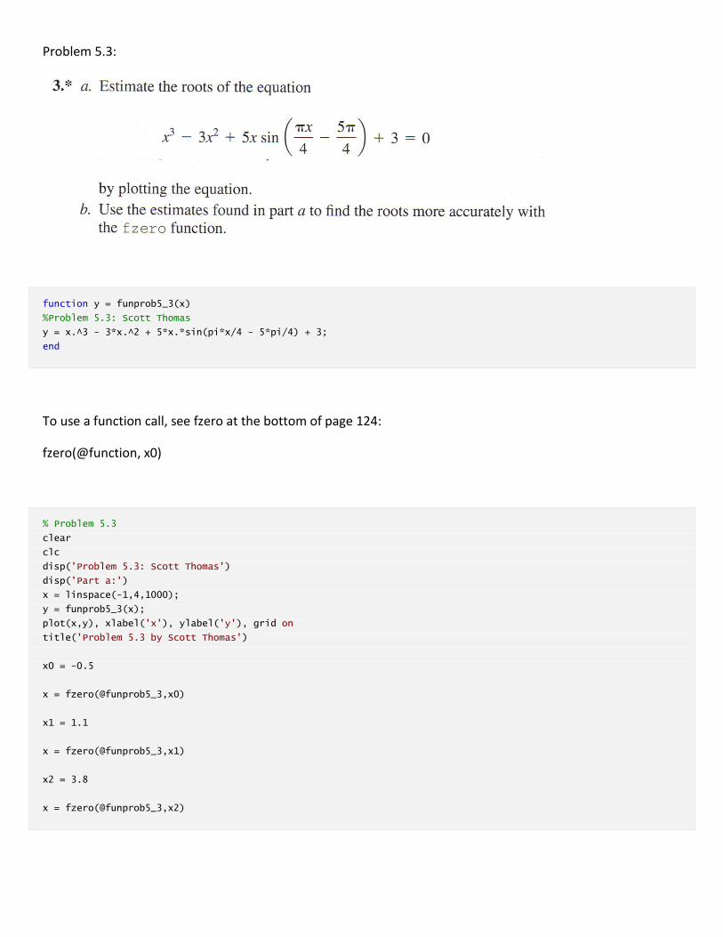
Problem 5.3:
function y = funprob5_3(x)
%Problem 5.3: Scott Thomas
y = x.^3 - 3*x.^2 + 5*x.*sin(pi*x/4 - 5*pi/4) + 3;
end
To use a function call, see fzero at the bottom of page 124:
fzero(@function, x0)
% Problem 5.3
clear
clc
disp('Problem 5.3: Scott Thomas')
disp('Part a:')
x = linspace(-1,4,1000);
y = funprob5_3(x);
plot(x,y), xlabel('x'), ylabel('y'), grid on
title('Problem 5.3 by Scott Thomas')
x0 = -0.5
x = fzero(@funprob5_3,x0)
x1 = 1.1
x = fzero(@funprob5_3,x1)
x2 = 3.8
x = fzero(@funprob5_3,x2)
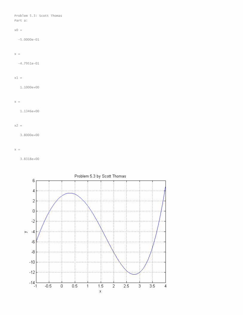
Problem 5.3: Scott Thomas
Part a:
x0 =
-5.0000e-01
x =
-4.7951e-01
x1 =
1.1000e+00
x =
1.1346e+00
x2 =
3.8000e+00
x =
3.8318e+00

Problem 5.6:
function V = funprob5_6(t)
V = 10^9 + 10^8*(1 - exp(-t/100)) - 10^7*t;
end
% Problem 5.6
clear
clc
disp('Problem 5.6: Scott Thomas')
xmin = 0;
xmax = 100;
fnc = @funprob5_6;
fplot(fnc,[xmin xmax]),xlabel('Time (days)'), ylabel('Reservoir Water Volume (liters)'),grid on
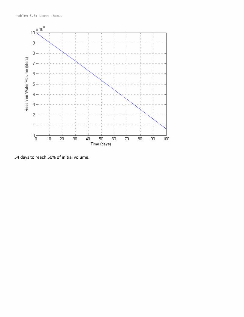
Problem 5.6: Scott Thomas
54 days to reach 50% of initial volume.
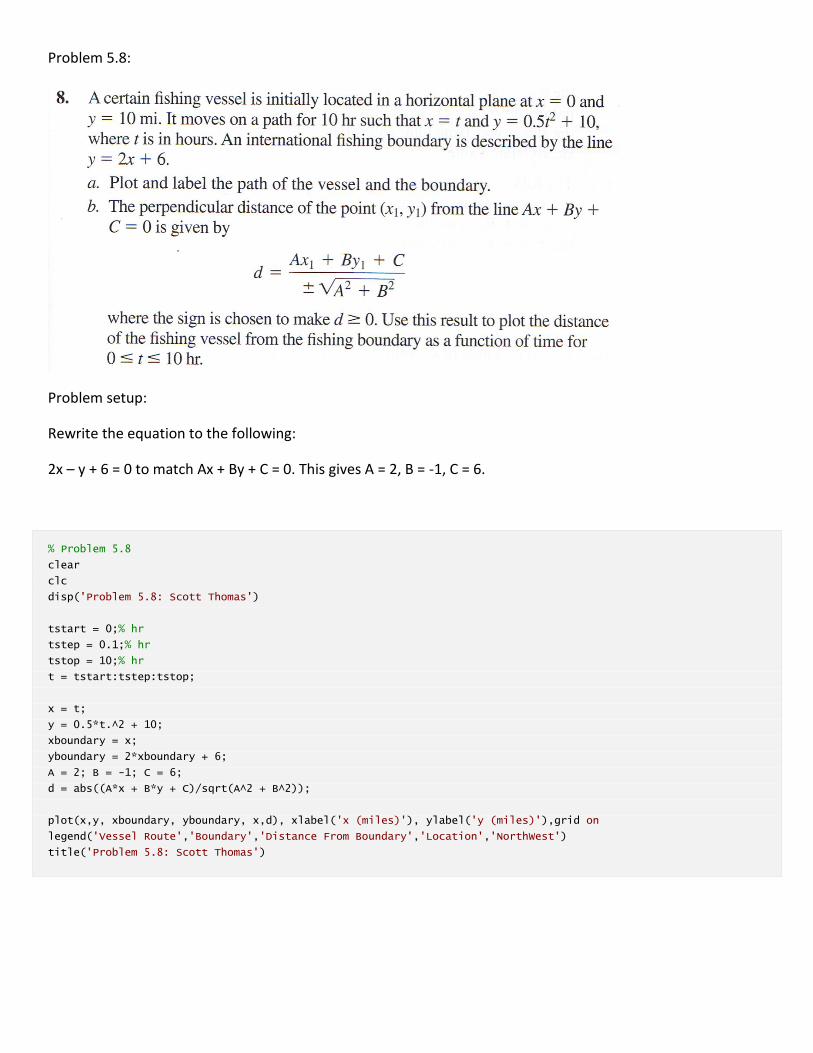
Problem 5.8:
Problem setup:
Rewrite the equation to the following:
2x – y + 6 = 0 to match Ax + By + C = 0. This gives A = 2, B = -1, C = 6.
% Problem 5.8
clear
clc
disp('Problem 5.8: Scott Thomas')
tstart = 0;% hr
tstep = 0.1;% hr
tstop = 10;% hr
t = tstart:tstep:tstop;
x = t;
y = 0.5*t.^2 + 10;
xboundary = x;
yboundary = 2*xboundary + 6;
A = 2; B = -1; C = 6;
d = abs((A*x + B*y + C)/sqrt(A^2 + B^2));
plot(x,y, xboundary, yboundary, x,d), xlabel('x (miles)'), ylabel('y (miles)'),grid on
legend('Vessel Route','Boundary','Distance From Boundary','Location','NorthWest')
title('Problem 5.8: Scott Thomas')

Problem 5.8: Scott Thomas
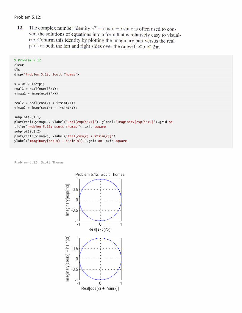
Problem 5.12:
% Problem 5.12
clear
clc
disp('Problem 5.12: Scott Thomas')
x = 0:0.01:2*pi;
real1 = real(exp(i*x));
yimag1 = imag(exp(i*x));
real2 = real(cos(x) + i*sin(x));
yimag2 = imag(cos(x) + i*sin(x));
subplot(2,1,1)
plot(real1,yimag1), xlabel('Real[exp(i*x)]'), ylabel('Imaginary[exp(i*x)]'),grid on
title('Problem 5.12: Scott Thomas'), axis square
subplot(2,1,2)
plot(real2,yimag2), xlabel('Real[cos(x) + i*sin(x)]')
ylabel('Imaginary[cos(x) + i*sin(x)]'),grid on, axis square
Problem 5.12: Scott Thomas
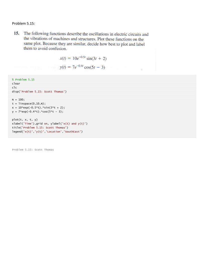
Problem 5.15:
% Problem 5.15
clear
clc
disp('Problem 5.15: Scott Thomas')
N = 100;
t = linspace(0,10,N);
x = 10*exp(-0.5*t).*sin(3*t + 2);
y = 7*exp(-0.4*t).*cos(5*t - 3);
plot(t, x, t, y)
xlabel('Time'),grid on, ylabel('x(t) and y(t)')
title('Problem 5.15: Scott Thomas')
legend('x(t)','y(t)','Location','SouthEast')
Problem 5.15: Scott Thomas


Problem 5.18:
% Problem 5.18
clear
clc
disp('Problem 5.18: Scott Thomas')
R = 286.7;% J/(kg-K)
T = 293;% degrees Kelvin
N = 1000;
V = linspace(20,100,N);% m^3
m = [1 3 7];% kg
p1 = m(1)*R*T./V;% (N/m^2)
p2 = m(2)*R*T./V;% (N/m^2)
p3 = m(3)*R*T./V;% (N/m^2)
plot(V, p1, V, p2, V, p3)
xlabel('Volume (m^3)'),grid on, ylabel('Pressure (N/m^2)')
legend('m = 1 kg','m = 3 kg','m = 7 kg','Location','NorthEast')
title('Problem 5.18: Scott Thomas')

Problem 5.18: Scott Thomas
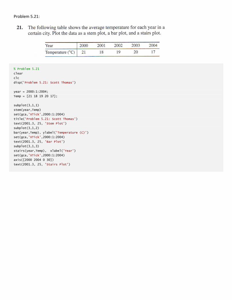
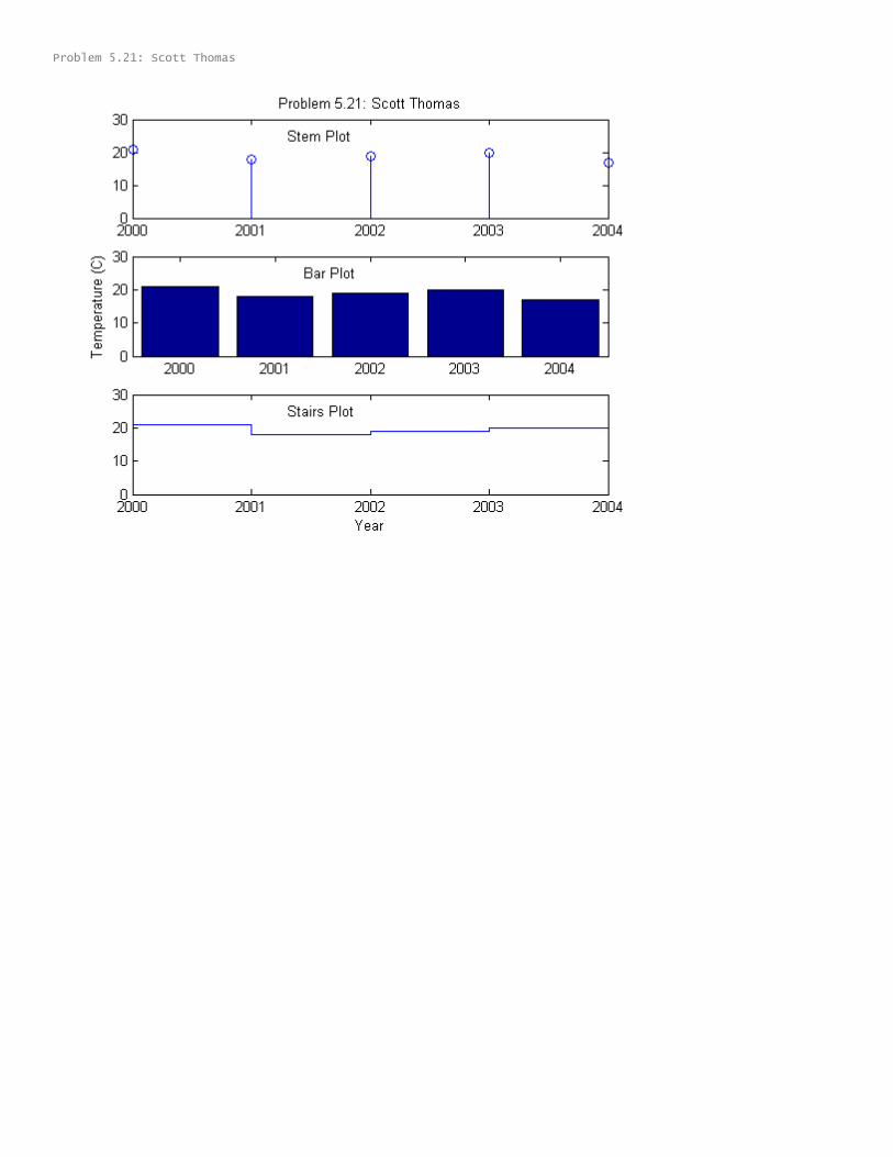
Problem 5.21:
% Problem 5.21
clear
clc
disp('Problem 5.21: Scott Thomas')
year = 2000:1:2004;
Temp = [21 18 19 20 17];
subplot(3,1,1)
stem(year,Temp)
set(gca,'XTick',2000:1:2004)
title('Problem 5.21: Scott Thomas')
text(2001.3, 25, 'Stem Plot')
subplot(3,1,2)
bar(year,Temp), ylabel('Temperature (C)')
set(gca,'XTick',2000:1:2004)
text(2001.3, 25, 'Bar Plot')
subplot(3,1,3)
stairs(year,Temp), xlabel('Year')
set(gca,'XTick',2000:1:2004)
axis([2000 2004 0 30])
text(2001.3, 25, 'Stairs Plot')
Problem 5.21: Scott Thomas

Problem 5.26:
% Problem 5.26
clear
clc
disp('Problem 5.26: Scott Thomas')
RC = 0.1;% seconds
N = 1000;
omega = logspace(0,2,N);
ratio = abs(1./(RC*omega.*(1i) + 1));
%
%semilogy
loglog(omega,ratio)
ylabel('|A_o/A_i|'), xlabel('\omega (1/sec = Hz)')
title('Problem 5.26: Scott Thomas')
set(gca,'YTick',linspace(0.1,1,10))
grid on
%legend('n = 1', 'n = 4', 'n = 12', 'Location', 'NorthWest')

Problem 5.26: Scott Thomas
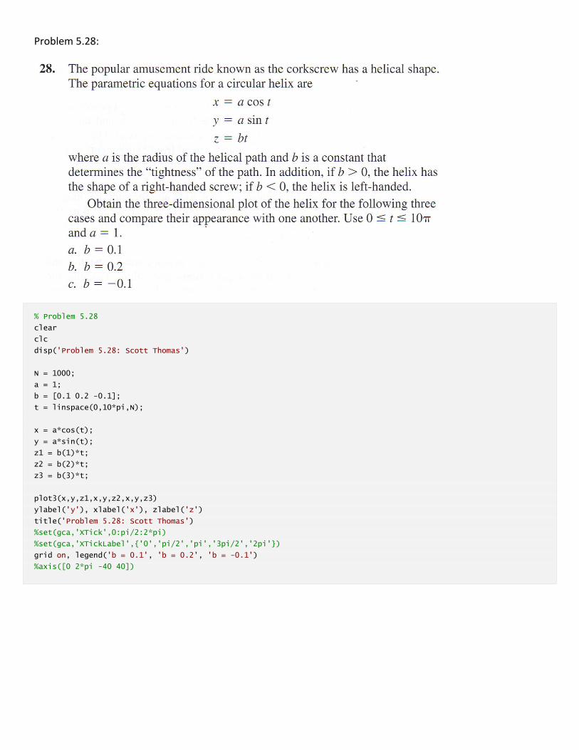
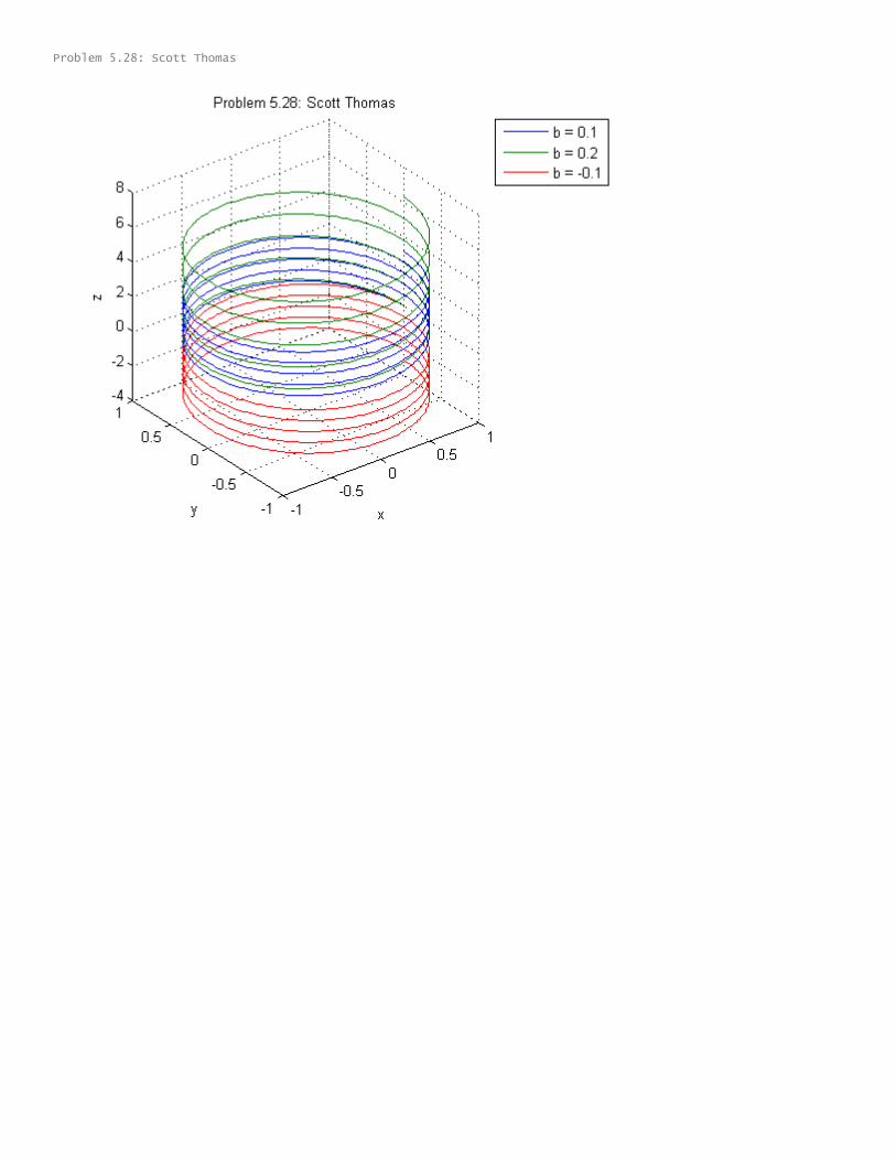
Problem 5.28:
% Problem 5.28
clear
clc
disp('Problem 5.28: Scott Thomas')
N = 1000;
a = 1;
b = [0.1 0.2 -0.1];
t = linspace(0,10*pi,N);
x = a*cos(t);
y = a*sin(t);
z1 = b(1)*t;
z2 = b(2)*t;
z3 = b(3)*t;
plot3(x,y,z1,x,y,z2,x,y,z3)
ylabel('y'), xlabel('x'), zlabel('z')
title('Problem 5.28: Scott Thomas')
%set(gca,'XTick',0:pi/2:2*pi)
%set(gca,'XTickLabel',{'0','pi/2','pi','3pi/2','2pi'})
grid on, legend('b = 0.1', 'b = 0.2', 'b = -0.1')
%axis([0 2*pi -40 40])
Problem 5.28: Scott Thomas

Problem 5.30:
% Problem 5.30
clear
clc
disp('Problem 5.30: Scott Thomas')
N = 30;
x = linspace(-10,10,N);
y = linspace(-10,10,N);
[X,Y] = meshgrid(x,y);
Z = X.^2 - 2*X.*Y + 4*Y.^2;
mesh(X,Y,Z)
%contour(X,Y,Z)
ylabel('y'), xlabel('x'), zlabel('z')
title('Problem 5.30: Scott Thomas')
grid on
Problem 5.30: Scott Thomas
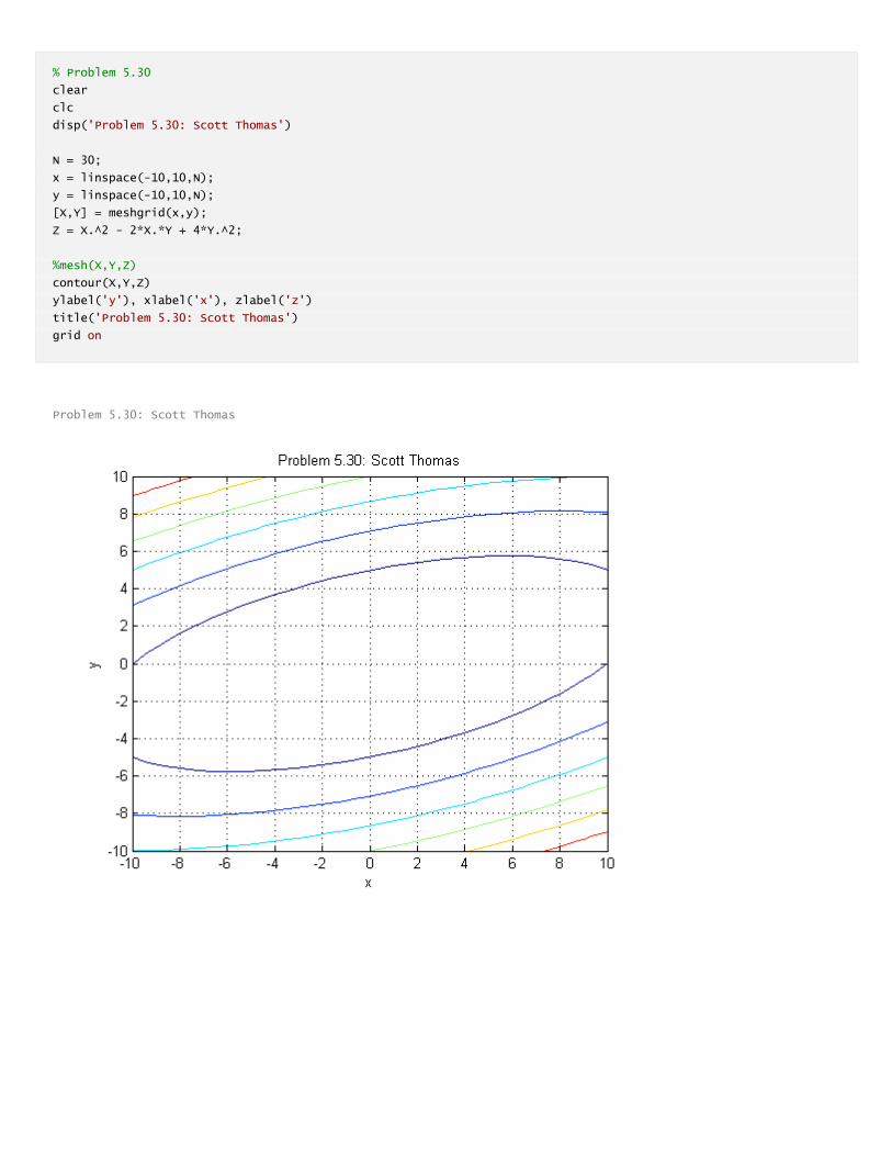
% Problem 5.30
clear
clc
disp('Problem 5.30: Scott Thomas')
N = 30;
x = linspace(-10,10,N);
y = linspace(-10,10,N);
[X,Y] = meshgrid(x,y);
Z = X.^2 - 2*X.*Y + 4*Y.^2;
%mesh(X,Y,Z)
contour(X,Y,Z)
ylabel('y'), xlabel('x'), zlabel('z')
title('Problem 5.30: Scott Thomas')
grid on
Problem 5.30: Scott Thomas