Matrix Factorization and FactorizationMachines for Recommender Systems
Chih-Jen LinDepartment of Computer Science
National Taiwan University
Talk at 4th Workshop on Large-Scale Recommender Systems,
ACM RecSys, 2016Chih-Jen Lin (National Taiwan Univ.) 1 / 47

Outline
1 Matrix factorization
2 Factorization machines
3 Field-aware factorization machines
4 Optimization methods for large-scale training
5 Discussion and conclusions
Chih-Jen Lin (National Taiwan Univ.) 2 / 47

Matrix factorization
Outline
1 Matrix factorization
2 Factorization machines
3 Field-aware factorization machines
4 Optimization methods for large-scale training
5 Discussion and conclusions
Chih-Jen Lin (National Taiwan Univ.) 3 / 47

Matrix factorization
Matrix Factorization
Matrix Factorization is an effective method forrecommender systems (e.g., Netflix Prize and KDDCup 2011)A group of users give ratings to some items
User Item Rating1 5 1001 13 30. . . . . . . . .u v r. . . . . . . . .
The information can be represented by a ratingmatrix R
Chih-Jen Lin (National Taiwan Univ.) 4 / 47

Matrix factorization
Matrix Factorization (Cont’d)
R
m × n
m
:
u
:2
1
1 2 .. v .. .. .. n
ru,v
?2,2
m, n: numbers of users and items
u, v : index for uth user and vth item
ru,v : uth user gives a rating ru,v to vth itemChih-Jen Lin (National Taiwan Univ.) 5 / 47

Matrix factorization
Matrix Factorization (Cont’d)
R
m × n
≈ ×
PT
m × k
Q
k × n
m:u:21
1 2 .. v .. .. .. n
ruv
?2,2
pT1
pT2
:
pTu
:
pTm
q1 q2 .. qv .. .. .. qn
k : number of latent dimensions
ru,v = pTu qv
?2,2 = pT2 q2
Chih-Jen Lin (National Taiwan Univ.) 6 / 47

Matrix factorization
Matrix Factorization (Cont’d)
A non-convex optimization problem:
minP,Q
∑(u,v)∈R
((ru,v − pT
u qv)2 + λP ‖pu‖2F + λQ ‖qv‖2F)
λP and λQ are regularization parameters
Many optimization methods have been successfullyapplied
Overall MF is a mature technique
Chih-Jen Lin (National Taiwan Univ.) 7 / 47
Factorization machines
Outline
1 Matrix factorization
2 Factorization machines
3 Field-aware factorization machines
4 Optimization methods for large-scale training
5 Discussion and conclusions
Chih-Jen Lin (National Taiwan Univ.) 8 / 47
Factorization machines
MF versus Classification/Regression
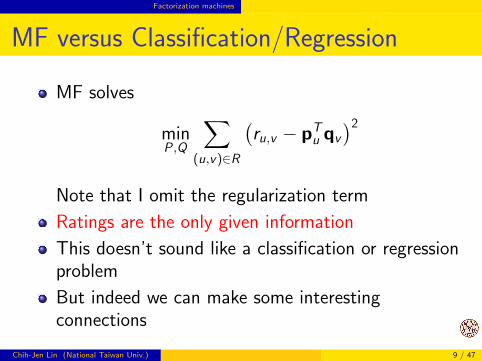
MF solves
minP,Q
∑(u,v)∈R
(ru,v − pT
u qv
)2Note that I omit the regularization term
Ratings are the only given information
This doesn’t sound like a classification or regressionproblem
But indeed we can make some interestingconnections
Chih-Jen Lin (National Taiwan Univ.) 9 / 47
Factorization machines
Handling User/Item Features
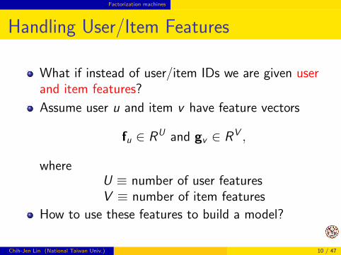
What if instead of user/item IDs we are given userand item features?
Assume user u and item v have feature vectors
fu ∈ RU and gv ∈ RV ,
whereU ≡ number of user featuresV ≡ number of item features
How to use these features to build a model?
Chih-Jen Lin (National Taiwan Univ.) 10 / 47

Factorization machines
Handling User/Item Features (Cont’d)
We can consider a regression problem where datainstances are
value features...
...ruv
[fTu gT
v
]...
...
and solve
minw
∑u,v∈R
(ru,v −wT
[fugv
])2
Chih-Jen Lin (National Taiwan Univ.) 11 / 47

Factorization machines
Feature Combinations
However, this does not take the interaction betweenusers and items into account
Following the concept of degree-2 polynomialmappings in SVM, we can generate new features
(fu)t(gv)s , t = 1, . . . ,U , s = 1, . . .V
and solve
minwt,s ,∀t,s
∑u,v∈R
(ru,v −U∑t=1
V∑s=1
wt,s(fu)t(gv)s)2
Chih-Jen Lin (National Taiwan Univ.) 12 / 47
Factorization machines
Feature Combinations (Cont’d)
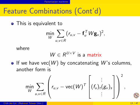
This is equivalent to
minW
∑u,v∈R
(ru,v − fTu Wgv)2,
whereW ∈ RU×V is a matrix
If we have vec(W ) by concatenating W ’s columns,another form is
minW
∑u,v∈R
ru,v − vec(W )T
...(fu)t(gv)s
...
2
,
Chih-Jen Lin (National Taiwan Univ.) 13 / 47

Factorization machines
Feature Combinations (Cont’d)
However, this setting fails for extremely sparsefeatures
Consider the most extreme situation. Assume wehave
user ID and item ID
as features
Then
U = m, J = n,
fi = [0, . . . , 0︸ ︷︷ ︸i−1
, 1, 0, . . . , 0]T
Chih-Jen Lin (National Taiwan Univ.) 14 / 47

Factorization machines
Feature Combinations (Cont’d)
The optimal solution is
Wu,v =
{ru,v , if u, v ∈ R
0, if u, v /∈ R
We can never predict
ru,v , u, v /∈ R
Chih-Jen Lin (National Taiwan Univ.) 15 / 47
Factorization machines
Factorization Machines
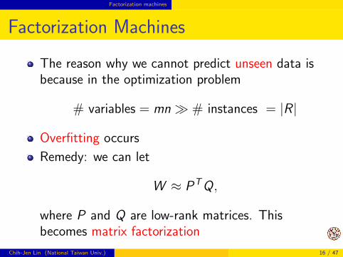
The reason why we cannot predict unseen data isbecause in the optimization problem
# variables = mn� # instances = |R |
Overfitting occurs
Remedy: we can let
W ≈ PTQ,
where P and Q are low-rank matrices. Thisbecomes matrix factorization
Chih-Jen Lin (National Taiwan Univ.) 16 / 47
Factorization machines
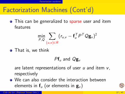
Factorization Machines (Cont’d)
This can be generalized to sparse user and itemfeatures
minP,Q
∑(u,v)∈R
(ru,v − fTu PTQgv)2
That is, we think
Pfu and Qgv
are latent representations of user u and item v ,respectivelyWe can also consider the interaction betweenelements in fu (or elements in gv)
Chih-Jen Lin (National Taiwan Univ.) 17 / 47
Factorization machines
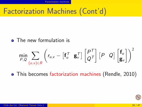
Factorization Machines (Cont’d)
The new formulation is
minP,Q
∑(u,v)∈R
(ru,v −
[fTu gT
v
] [PT
QT
] [P Q
] [ fugv
])2
This becomes factorization machines (Rendle, 2010)
Chih-Jen Lin (National Taiwan Univ.) 18 / 47
Factorization machines
Factorization Machines (Cont’d)
Similar ideas have been used in other places such asStern et al. (2009)
We see that such ideas can be used for not onlyrecommender systems.
They may be useful for any classification problemswith very sparse features
Chih-Jen Lin (National Taiwan Univ.) 19 / 47

Factorization machines
FM for Classification
In a classification setting assume a data instance isx ∈ Rn
Linear model:wTx
Degree-2 polynomial mapping:
xTW x
Chih-Jen Lin (National Taiwan Univ.) 20 / 47

Factorization machines
FM for Classification (Cont’d)
FM:xTPTPx
or alternatively ∑i ,j
xipTi pjxj ,
wherepi ,pj ∈ Rk
That is, in FM each feature is associated with alatent factor
Chih-Jen Lin (National Taiwan Univ.) 21 / 47

Field-aware factorization machines
Outline
1 Matrix factorization
2 Factorization machines
3 Field-aware factorization machines
4 Optimization methods for large-scale training
5 Discussion and conclusions
Chih-Jen Lin (National Taiwan Univ.) 22 / 47
Field-aware factorization machines
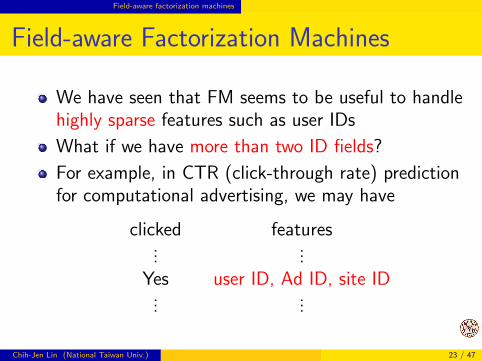
Field-aware Factorization Machines
We have seen that FM seems to be useful to handlehighly sparse features such as user IDs
What if we have more than two ID fields?
For example, in CTR (click-through rate) predictionfor computational advertising, we may have
clicked features...
...Yes user ID, Ad ID, site ID
......
Chih-Jen Lin (National Taiwan Univ.) 23 / 47
Field-aware factorization machines
Field-aware Factorization Machines(Cont’d)
FM can be generalized to handle differentinteractions between fields
Two latent matrices for user ID and Ad IDTwo latent matrices for user ID and site ID...
We call this approach FFM (field-aware factorizationmachines)
An early study on three fields is Rendle andSchmidt-Thieme (2010)
Chih-Jen Lin (National Taiwan Univ.) 24 / 47

Field-aware factorization machines
FFM for CTR Prediction
It’s used by Jahrer et al. (2012) to win the 2nd prizeof KDD Cup 2012
In 2014 my students used FFM to win two KaggleCTR competitions
After we used FFM to win the first competition, inthe second competition all top teams use FFM
Note that for CTR prediction, logistic rather thansquared loss is used
Chih-Jen Lin (National Taiwan Univ.) 25 / 47

Field-aware factorization machines
Practical Use of FFM
Recently we conducted a detailed study on FFM(Juan et al., 2016)
Here I briefly discuss some results there
Chih-Jen Lin (National Taiwan Univ.) 26 / 47
Field-aware factorization machines
Numerical Features
For categorical features like IDs, we have
ID: field ID index: feature
Each field has many 0/1 features
But how about numerical features?
Two possibilities
Dummy fields: The field has only onereal-valued featureDiscretization: transform a numerical feature toa categorical one and then many binary features
Chih-Jen Lin (National Taiwan Univ.) 27 / 47
Field-aware factorization machines
Normalization
After obtaining the feature vector, empirically wefind that instance-wise normalization is useful
Faster convergence and better test accuracy
Chih-Jen Lin (National Taiwan Univ.) 28 / 47

Field-aware factorization machines
Impact of Parameters
We have the following parameters
k : number of latent factors
λ: regularization parameter
parameters of the optimization methods (e.g.,learning rate of stochastic gradient)
Their sensitivity to the performance varies
Chih-Jen Lin (National Taiwan Univ.) 29 / 47

Field-aware factorization machines
Example: Regularization Parameter λ
Epochs20 40 60 80 100 120 140
Logloss
0.44
0.45
0.46
0.47
0.48
0.49
0.5λ = 1e− 6
λ = 1e− 5
λ = 1e− 4
λ = 1e− 3
Too large λ: model not goodToo small λ: better model but easily overfittingSimilar situations occur for SG learning ratesEarly stopping by a validation procedure is needed
Chih-Jen Lin (National Taiwan Univ.) 30 / 47
Field-aware factorization machines
Experiments: Two CTR Sets
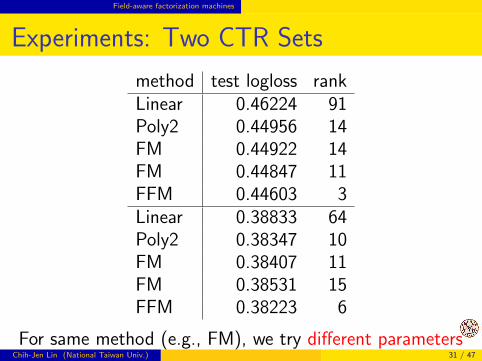
method test logloss rankLinear 0.46224 91Poly2 0.44956 14FM 0.44922 14FM 0.44847 11FFM 0.44603 3Linear 0.38833 64Poly2 0.38347 10FM 0.38407 11FM 0.38531 15FFM 0.38223 6
For same method (e.g., FM), we try different parametersChih-Jen Lin (National Taiwan Univ.) 31 / 47

Field-aware factorization machines
Experiments: Two CTR Sets (Cont’d)
For these two sets, FFM is the best
For winning competitions, some additional tricks areused
Chih-Jen Lin (National Taiwan Univ.) 32 / 47
Field-aware factorization machines
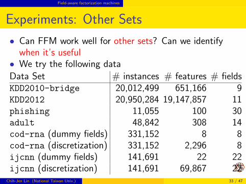
Experiments: Other Sets
• Can FFM work well for other sets? Can we identifywhen it’s useful• We try the following data
Data Set # instances # features # fieldsKDD2010-bridge 20,012,499 651,166 9KDD2012 20,950,284 19,147,857 11phishing 11,055 100 30adult 48,842 308 14cod-rna (dummy fields) 331,152 8 8cod-rna (discretization) 331,152 2,296 8ijcnn (dummy fields) 141,691 22 22ijcnn (discretization) 141,691 69,867 22
Chih-Jen Lin (National Taiwan Univ.) 33 / 47

Field-aware factorization machines
Experiments: Other Sets (Cont’d)
Data Set LM Poly2 FM FFMKDD2010-bridge 0.30910 0.27448 0.28437 0.26899KDD2012 0.49375 0.49640 0.49292 0.48700phishing 0.11493 0.09659 0.09461 0.09374adult 0.30897 0.30757 0.30959 0.30760cod-rna (dummy fields) 0.13829 0.12874 0.12580 0.12914cod-rna (discretization) 0.16455 0.17576 0.16570 0.14993ijcnn (dummy fields) 0.20627 0.09209 0.07696 0.07668ijcnn (discretization) 0.21686 0.22546 0.22259 0.18635
Best results are underlined
Chih-Jen Lin (National Taiwan Univ.) 34 / 47

Field-aware factorization machines
Experiments: Other Sets (Cont’d)
For data with categorical data, FFM works well
For some data (e.g., adult), feature interactionsare not useful
It’s not easy for FFM to handle numerical features
Chih-Jen Lin (National Taiwan Univ.) 35 / 47

Optimization methods for large-scale training
Outline
1 Matrix factorization
2 Factorization machines
3 Field-aware factorization machines
4 Optimization methods for large-scale training
5 Discussion and conclusions
Chih-Jen Lin (National Taiwan Univ.) 36 / 47
Optimization methods for large-scale training
Solving the Optimization Problem
MF, FM, and FFM all involve optimization problems
Optimization techniques for them are related butdifferent due to different problem structures
With time constraint I will only briefly discuss someoptimization techniques for matrix factorization
Chih-Jen Lin (National Taiwan Univ.) 37 / 47
Optimization methods for large-scale training
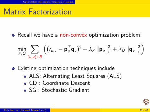
Matrix Factorization
Recall we have a non-convex optimization problem:
minP,Q
∑(u,v)∈R
((ru,v − pT
u qv)2 + λP ‖pu‖2F + λQ ‖qv‖2F)
Existing optimization techniques include
ALS: Alternating Least Squares (ALS)CD : Coordinate DescentSG : Stochastic Gradient
Chih-Jen Lin (National Taiwan Univ.) 38 / 47

Optimization methods for large-scale training
Complexity in Training MF
To update P ,Q once
ALS: O(|R |k2 + (m + n)k3)
CD: O(|R |k)
To go through |R | elements once
SG: O(|R |k)
I don’t discuss details, but this indicates that CD and SGare generally more efficient
Chih-Jen Lin (National Taiwan Univ.) 39 / 47
Optimization methods for large-scale training
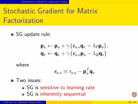
Stochastic Gradient for MatrixFactorization
SG update rule:
pu ← pu + γ (eu,vqv − λPpu) ,
qv ← qv + γ (eu,vpu − λQqv)
whereeu,v ≡ ru,v − pT
u qv
Two issues:
SG is sensitive to learning rateSG is inherently sequential
Chih-Jen Lin (National Taiwan Univ.) 40 / 47

Optimization methods for large-scale training
SG’s Learning Rate
We can apply advanced settings such as ADAGRAD(Duchi et al., 2011)
Each element of latent vectors pu, qv has its ownlearning rate
Maintaining so many learning rates can be quiteexpensive
How about a modification to let the whole pu (orthe whole qv) associates with a rate? (Chin et al.,2015b)
This is an example that we take MF’s property intoaccount
Chih-Jen Lin (National Taiwan Univ.) 41 / 47
Optimization methods for large-scale training
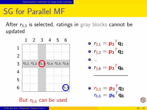
SG for Parallel MF
After r3,3 is selected, ratings in gray blocks cannot beupdated
r3,1 r3,2 r3,3 r3,4 r3,5 r3,6
r6,6
1 2 3 4 5 6
1
2
3
4
5
6
But r6,6 can be used
r3,1 = p3Tq1
r3,2 = p3Tq2
..
r3,6 = p3Tq6
——————
r3,3 = p3Tq3
r6,6 = p6Tq6
Chih-Jen Lin (National Taiwan Univ.) 42 / 47

Optimization methods for large-scale training
SG for Parallel MF (Cont’d)
We can split the matrix to blocks and update thosewhich don’t share p or q
1 2 3 4 5 6
1
2
3
4
5
6
This concept is simple, but there are many issues to havea right implementation under the given architecture
Chih-Jen Lin (National Taiwan Univ.) 43 / 47

Optimization methods for large-scale training
SG for Parallel MF (Cont’d)
Past developments of SG for parallel MF includeGemulla et al. (2011); Chin et al. (2015a); Yunet al. (2014)
However, the idea of block splits applies to MF only
We haven’t seen an easy way to extend it to FM orFFM
This is another example where we take problemstructure into account
Chih-Jen Lin (National Taiwan Univ.) 44 / 47

Discussion and conclusions
Outline
1 Matrix factorization
2 Factorization machines
3 Field-aware factorization machines
4 Optimization methods for large-scale training
5 Discussion and conclusions
Chih-Jen Lin (National Taiwan Univ.) 45 / 47
Discussion and conclusions
Discussion and Conclusions
In this talk we briefly discuss three models forrecommender systems
MF, FM, and FFM
They are related, but are useful in differentsituations
Different algorithms may be needed due to differentproperties of the optimization problems
Chih-Jen Lin (National Taiwan Univ.) 46 / 47

Discussion and conclusions
Acknowledgments
Past and current students who have contributed to thiswork:
Wei-Sheng Chin
Yu-Chin Juan
Meng-Yuan Yang
Bo-Wen Yuan
Yong Zhuang
We thank the support from Ministry of Science andTechnology in Taiwan
Chih-Jen Lin (National Taiwan Univ.) 47 / 47


![Robust Factorization Machines for User Response Predictionwnzhang.net/share/rtb-papers/rfm- · Factorization machines (FMs) proposed in [22] have recently gained popularity as an](https://static.cupdf.com/doc/110x72/5ed73068c30795314c175d04/robust-factorization-machines-for-user-response-factorization-machines-fms-proposed.jpg)


![Factorization Machines with libFMb97053/paper/Factorization...Factorization Machines with libFM 57:3 Fig. 1. Example (from Rendle [2010]) for representing a recommender problem with](https://static.cupdf.com/doc/110x72/5e671c5cbd644c7e8d06c310/factorization-machines-with-libfm-b97053paperfactorization-factorization-machines.jpg)