Mathematical Models of Malaria Control withArtificial Feeders, Odorants and Bed Nets
by
Pius Ariho
BSc with Educ., Mbarara University, 2007
A Dissertation Submitted in Partial Fulfillment of theRequirements for the Degree of
Doctor of Philosophy
in the Graduate Academic Unit ofMathematics and Statistics
Supervisor: James Watmough, PhD, Dept. of Math & StatsExamining Board: Lin Wang, PhD, Dept. of Math & Stats
Sanjeev Seahra, PhD, Dept. of Math & StatsPaul Peters, PhD, Dept. of SociologyJohn Kershaw, PhD, SGS, Chairperson
External Examiner: Abba Gumel, PhD, Arizona State University
This dissertation is accepted by theDean of Graduate Studies
THE UNIVERSITY OF NEW BRUNSWICK
September, 2015
c©Pius Ariho, 2015
Abstract
Vector behaviour influences the speed of disease spread in populations. The
presence of vector bias towards hosts with special characteristics suggests
the need for new or tactical disease-control approaches. Malaria parasites
produce volatile mosquito attractants. As a result, mosquitoes have bias
towards malaria-infected humans. The control of mosquito-borne diseases
can be improved by targeting mosquito bias. The attractiveness of humans to
mosquitoes can be masked using appropriate odorants. Further, vectors can
be artificially blood-fed using simplified devices to prevent infectious bites.
In this study, we focus on the use of mosquito feeders, mosquito attractants,
repellents and bed nets, knowing that such a multifaceted approach has not
been explored previously using mathematical models.
Three models of malaria control are developed using systems of nonlinear
differential equations. The models are based on the Ross-Macdonald Theory
and recent studies of vector-host interactions. In the artificial-feeder model,
all infected humans acquire protective odorants at the onset of the infectious
stage. The model is analyzed to examine the effect of repellents and artificial
ii

feeders on disease transmission and spread. The second model is without
artificial feeders and assumes that infected individuals are recruited to use
protective odorants during the infectious stage. The resulting mosquito-bias
model is analyzed to examine how the recruitment rate affects disease spread.
The third model combines the use of artificial feeders and protective odorants
with the use of bed nets. The resulting bed-net model is analyzed to examine
the effect of bed nets and protective odorants on disease transmission and
spread in the presence of artificial feeders.
The results of this study suggest that artificial feeders can slow disease
spread, but eradication is easily done if mosquito bias is increased towards
uninfected individuals. Increasing repellent-usage during the infectious stage
decreases disease spread. The disease persists if mosquitoes are less attracted
to bed-net users than to non-users. The conclusion is that the transmis-
sion and spread of mosquito-borne pathogens can be stopped by using arti-
ficial feeders that are attractive to mosquitoes, by increasing repellent-usage
throughout the infectious stage, and by ensuring optimal bed-net coverage
with protective odorants for all bed-net non-users.
iii

Dedication
I dedicate this dissertation to my wife, Claire Kesande, and my children,
Achilles and Albert, who missed me so much and sacrificed a lot for me
when I was a PhD student.
iv

Acknowledgements
I would like to give thanks and appreciation to Professor James Watmough,
my supervisor, for being a tremendous mentor for me. I thank him for guiding
me, for teaching me Mathematical Biology, for encouraging my research and
for allowing me to grow as a research scientist.
I thank Lin Wang for teaching me Differential Equations, and Sanjeev
Seahra for teaching me Numerical Methods using MAPLE. I thank my Oral
Examination Committee: James Watmough, Lin Wang, Sanjeev Seahra,
Paul Peters, Abba Gumel and John Kershaw (Chairperson), for reading my
dissertation, for their brilliant comments and suggestions, and for letting my
oral defence be an enjoyable moment.
I thank Julius Tumwiine, for introducing me to Biomathematics, and
for being kind and supportive. I also thank the School of Graduate Studies
and the Department of Mathematics and Statistics at the University of New
Brunswick, for supporting me. I thank Nilmika and Patricia for proofreading
my drafts. Finally, I would like to thank my Classmates, Family and Friends.
Your prayers and support are what sustained me thus far.
v

Table of Contents
Abstract ii
Dedication iv
Acknowledgments v
Table of Contents viii
List of Tables ix
List of Figures x
1 Introduction 1
1.1 Introduction . . . . . . . . . . . . . . . . . . . . . . . . . . . . 1
1.2 Epidemiological Background . . . . . . . . . . . . . . . . . . . 9
1.3 Mathematics for Malaria control . . . . . . . . . . . . . . . . . 11
1.4 Mathematical Background . . . . . . . . . . . . . . . . . . . . 21
1.4.1 Basic system properties . . . . . . . . . . . . . . . . . . 21
1.4.2 Stability analysis . . . . . . . . . . . . . . . . . . . . . 24
1.4.3 Backward bifurcation . . . . . . . . . . . . . . . . . . . 27
vi

2 A mathematical model of Malaria control with artificial
feeders and protective odorants 29
2.1 Introduction . . . . . . . . . . . . . . . . . . . . . . . . . . . . 29
2.2 The artificial-feeder model . . . . . . . . . . . . . . . . . . . . 32
2.2.1 Model formulation . . . . . . . . . . . . . . . . . . . . 32
2.2.2 Well-posedness . . . . . . . . . . . . . . . . . . . . . . 37
2.3 Equilibria and their stability . . . . . . . . . . . . . . . . . . . 41
2.3.1 Disease-free equilibrium . . . . . . . . . . . . . . . . . 41
2.3.2 Endemic equilibria . . . . . . . . . . . . . . . . . . . . 46
2.3.3 Bifurcation analysis . . . . . . . . . . . . . . . . . . . . 52
2.4 Parameter values . . . . . . . . . . . . . . . . . . . . . . . . . 56
2.5 Discussion of results . . . . . . . . . . . . . . . . . . . . . . . 59
2.6 Concluding remarks . . . . . . . . . . . . . . . . . . . . . . . . 65
3 A mosquito-bias model with protective odorants for hosts
in the infectious stage 67
3.1 Introduction . . . . . . . . . . . . . . . . . . . . . . . . . . . . 67
3.2 The mosquito-bias model . . . . . . . . . . . . . . . . . . . . . 68
3.2.1 Model formulation . . . . . . . . . . . . . . . . . . . . 68
3.2.2 Well-posedness . . . . . . . . . . . . . . . . . . . . . . 74
3.3 Equilibria and their stability . . . . . . . . . . . . . . . . . . . 75
3.3.1 Disease-free equilibrium . . . . . . . . . . . . . . . . . 75
3.3.2 Endemic equilibria . . . . . . . . . . . . . . . . . . . . 79
vii

3.4 Results and discussion . . . . . . . . . . . . . . . . . . . . . . 82
3.5 Summary and conclusion . . . . . . . . . . . . . . . . . . . . . 88
4 A bed-net model for Malaria control with artificial feeders
and protective odorants 90
4.1 Introduction . . . . . . . . . . . . . . . . . . . . . . . . . . . . 90
4.2 The bed-net model . . . . . . . . . . . . . . . . . . . . . . . . 93
4.2.1 Model formulation . . . . . . . . . . . . . . . . . . . . 93
4.2.2 Rescaled bed-net model . . . . . . . . . . . . . . . . . 97
4.2.3 Well-posedness . . . . . . . . . . . . . . . . . . . . . . 101
4.3 Equilibria and their stability . . . . . . . . . . . . . . . . . . . 104
4.3.1 Disease-free equilibrium . . . . . . . . . . . . . . . . . 104
4.3.2 Endemic equilibria . . . . . . . . . . . . . . . . . . . . 109
4.3.3 Elasticity analysis of Rc . . . . . . . . . . . . . . . . . 112
4.4 Discussion of results . . . . . . . . . . . . . . . . . . . . . . . 114
4.5 Conclusion . . . . . . . . . . . . . . . . . . . . . . . . . . . . . 122
5 Results and Future work 124
5.1 Summary . . . . . . . . . . . . . . . . . . . . . . . . . . . . . 124
5.2 Results and Implications . . . . . . . . . . . . . . . . . . . . . 127
5.3 Future work . . . . . . . . . . . . . . . . . . . . . . . . . . . . 129
Bibliography 131
Vita
viii

List of Tables
2.1 Parameters for the artificial-feeder model . . . . . . . . . . . 36
2.2 Parameter values used for simulations . . . . . . . . . . . . . 59
3.1 Parameters for the mosquito-bias model . . . . . . . . . . . . 73
3.2 Parameter values used for simulations . . . . . . . . . . . . . 83
4.1 Parameters for the bed-net model . . . . . . . . . . . . . . . 100
4.2 Parameter values used for simulations . . . . . . . . . . . . . 115
List of Figures
1.1 Insect repellents . . . . . . . . . . . . . . . . . . . . . . . . . . 5
1.2 Schematic representation of the artificial feeder . . . . . . . . 5
1.3 Ceiling hung mosquito netting . . . . . . . . . . . . . . . . . . 6
1.4 Schematic diagram for malaria transmission dynamics . . . . . 16
2.1 Bifurcations in the c-A plane . . . . . . . . . . . . . . . . . . . 60
ix
2.2 Effect of A on subcritical bifurcation . . . . . . . . . . . . . . 61
2.3 Effect of c on I∗h with A negligible . . . . . . . . . . . . . . . . 62
2.4 Effect of c on I∗h with δh negligible . . . . . . . . . . . . . . . . 63
2.5 Stability of the disease-free equilibrium . . . . . . . . . . . . . 64
2.6 Stability of the endemic equilibrium . . . . . . . . . . . . . . . 64
3.1 Effect of odorant acquisition on Rc . . . . . . . . . . . . . . . 84
3.2 Bifurcations in the c-νp plane . . . . . . . . . . . . . . . . . . 85
3.3 Effect of c on I∗u . . . . . . . . . . . . . . . . . . . . . . . . . . 85
3.4 Stability of the disease-free equilibrium . . . . . . . . . . . . . 86
3.5 Stability of the endemic equilibrium . . . . . . . . . . . . . . . 87
4.1 Bifurcation in the φ-A plane . . . . . . . . . . . . . . . . . . . 116
4.2 Stability of the disease-free equilibrium . . . . . . . . . . . . . 117
4.3 Malaria prevalence for bed-net users (I1) . . . . . . . . . . . . 118
4.4 Malaria prevalence for bed-net non-users (I2) . . . . . . . . . . 118
4.5 Effect of φ on Rc with A negligible . . . . . . . . . . . . . . . 120
4.6 Effect of φ on Rc with A small . . . . . . . . . . . . . . . . . . 121
4.7 Effect of φ on Rc with A large . . . . . . . . . . . . . . . . . . 122
x

Chapter 1
Introduction
1.1 Introduction
The resurgence of vector-borne diseases presents a global health problem.
According to Gubler [37], the problem has come as a result of “changes
in public health policy, insecticide and drug resistance, shift in emphasis
from prevention to emergency response, demographic and societal changes,
and genetic changes in pathogens”. Every year there are more than one
billion cases and over one million deaths from vector-borne diseases such
as malaria, dengue, Chagas disease, yellow fever, plague, human African
trypanosomiasis (sleeping sickness), schistosomiasis, leishmaniasis, Japanese
encephalitis and onchocerciasis, globally (World Health Organization [112]).
Although the diseases are preventable through informed protective measures,
the resurgence suggests the need for more effective disease control approaches.
1

Vectors are living organisms that can transmit infectious diseases from
animals to humans or between humans. Many vectors are bloodsucking in-
sects, which ingest disease-producing pathogens during a blood meal from an
infected host and later inject them into a new host during a subsequent blood
meal. Vectors include mosquitoes, ticks, flies, triatomine bugs, sandflies, fleas
and some freshwater aquatic snails. Mosquitoes are the most common dis-
ease vectors. Mosquitoes transmit malaria, dengue, Rift Valley fever, yellow
fever, Chikungunya, lymphatic filariasis, Japanese encephalitis, and West
Nile fever through bites [94, 95, 77, 109, 112].
Vector behaviour influences the speed of disease spread among hosts.
Many studies of vector dynamics assume that vector-host interactions are
random. Evidence suggests that mosquitoes do not choose hosts randomly
[17, 52, 91, 93]. Carey and Carlson [17] suggest that a mosquito relies on its
sense of smell (olfaction) for locating food sources, hosts and egg-deposition
sites. A mosquito finds a host using chemical, visual, and thermal cues.
According to Tauxe et al. [101], a mosquito’s cpA neuron detector of skin and
carbon dioxide is used to locate humans. This dependence of host-selection
on mosquito behaviour and cues is called mosquito bias.
Malaria parasites produce volatile mosquito attractants [27, 45, 52, 93].
In a study by Lacroix et al [52], the presence of gametocytes in malaria-
infected children increased mosquito attraction. Considering the difference
between the proportions of the mosquitoes attracted to gametocyte carriers
before and after treatment, a statistical analysis suggested that mosquito
2
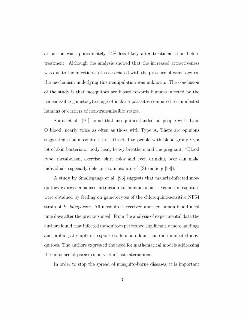
attraction was approximately 14% less likely after treatment than before
treatment. Although the analysis showed that the increased attractiveness
was due to the infection status associated with the presence of gametocytes,
the mechanism underlying this manipulation was unknown. The conclusion
of the study is that mosquitoes are biased towards humans infected by the
transmissible gametocyte stage of malaria parasites compared to uninfected
humans or carriers of non-transmissible stages.
Shirai et al. [91] found that mosquitoes landed on people with Type
O blood, nearly twice as often as those with Type A. There are opinions
suggesting that mosquitoes are attracted to people with blood group O, a
lot of skin bacteria or body heat, heavy breathers and the pregnant. “Blood
type, metabolism, exercise, shirt color and even drinking beer can make
individuals especially delicious to mosquitoes” (Stromberg [98]).
A study by Smallegange et al. [93] suggests that malaria-infected mos-
quitoes express enhanced attraction to human odour. Female mosquitoes
were obtained by feeding on gametocytes of the chloroquine-sensitive NF54
strain of P. falciparum. All mosquitoes received another human blood meal
nine days after the previous meal. From the analysis of experimental data the
authors found that infected mosquitoes performed significantly more landings
and probing attempts in response to human odour than did uninfected mos-
quitoes. The authors expressed the need for mathematical models addressing
the influence of parasites on vector-host interactions.
In order to stop the spread of mosquito-borne diseases, it is important
3

to influence mosquito bias. Mosquito bias can be influenced using protective
odorants such as mosquito attractants and insect repellents. Following [17],
Potter [83] asks whether a mosquito would still be able to target a human
host if it lacked its olfactory senses, and if odorants could be used to trick
the mosquito into avoiding humans! According to Potter, recent studies by
Tauxe et al. [101] and several others have started to address the answers.
The study by Tauxe et al. [101] suggests that a mosquito’s cpA dual
detector of skin odour and carbon dioxide can be blocked by an inhibitory
odorant, thus blocking attraction of mosquitoes to human skin. That said,
Potter [83] concludes that host seeking involves multiple sensory modalities,
and abolishing one sense might not be sufficient to completely eliminate
biting. To improve disease control, there is need to study and identify the
mechanisms by which other sensory cues are detected by the mosquito, and
the potential strategies to block them.
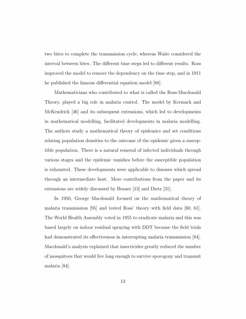
Insect repellents and other protective odorants (see Figure 1.1) can be
used to prevent bites. Further, mosquitoes can be artificially blood-fed to
prevent mosquito bites. It is known that animals can be used to blood-feed
mosquitoes but the practice has diminished due to the implementation of
strict guidelines governing the use of live animals (see Section 2.4.10 of MR4
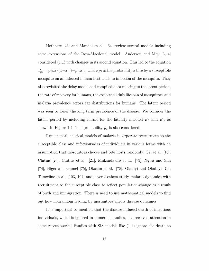
Staff [72]). Artificial feeders [26, 34] are simplified devices which can be
distributed in multiple places to provide blood meals to mosquitoes. They
include the recently developed “Glytube” [25] (see Figure 1.2) and mem-
brane feeders such as the Mishra feeder [67], the Mourya feeder [71], and the
4

Tseng feeder [102]. Further, artificial feeders can be treated with mosquito
attractants to increase the attractiveness of the feeders to mosquitoes.
Figure 1.1: Insect repellents. Left-Right: Off Family with aloe vera (cream),Nopikex (square soap with 22% Deet), Off Deep Woods (spray), BushmanPlus Water Resistant (80% Deet with sunscreen), Fly Out (pump spray),Mosquito F.O! (pump spray), and Bugs Lock (wrist/ankle bands).
system. Furthermore, other reports which published differentartificial feeders also just compared feeding efficiency in relation tolive animals [12,17,20].
Feeding efficiency is a relevant parameter which needs to beobserved in development of artificial feeder devices. Unfortunate-ly, the differences in experimental conditions between articles thatshowed other blood feeders are enormous and impose difficulties
Figure 1. Materials used to assemble the Glytube blood feeder device. A. A conical tube (50 mL) filled with 40 mL warmed 100% glyceroland top sealed with Dura Seal
TM
heat-resistant sealing film. The sealing film is laterally held to the tube using a Parafilm-MH thin strip (2.5 cm65.0 cm).B. Screw cap of the conical tube. Dashed circular black line indicates the cap region where plastic is removed by cutting to generate the feedingelement. C. Screw cap with 2.5 cm diameter hole. D. Screw cap covered externally with stretched Parafilm-M. A strip of Parafilm is fixing the feedingmembrane to the cap. E. A piece of Parafilm-M (5 cm65 cm) as a feeding membrane. Parafilm must be stretched to cover the screw cap. F. A piece ofDura Seal heat-resistant sealing film is used to sealing the conical tube filled with pre-heated 100% glycerol. G. Blood supplying the feeding elementat internal side of the screw cap with the stretched Parafilm membrane. H. Heating and feeding elements assembled together to feed the Ae. aegyptifemales. I. Non blood-fed (black arrowhead) and artificially blood-fed females with dilated abdomens (black arrows).doi:10.1371/journal.pone.0053816.g001
Figure 2. Schematic representation of the Glytube. A. Exploded drawing showing the materials used to prepare the device and elements orderto assemble the in-house feeder. B. View of assembled Glytube before mosquito feeding.doi:10.1371/journal.pone.0053816.g002
Novel Device to Blood-Feed Aedes aegypti
PLOS ONE | www.plosone.org 3 January 2013 | Volume 8 | Issue 1 | e53816
Figure 1.2: Schematic representation of the artificial feeder. Diagram Ashows the materials used to prepare the device and the order of assemblyof the feeder. Diagram B shows the assembled Glytube before mosquitofeeding. Source: Costa-da-Silva et al. (2013) [25], page 3.
5

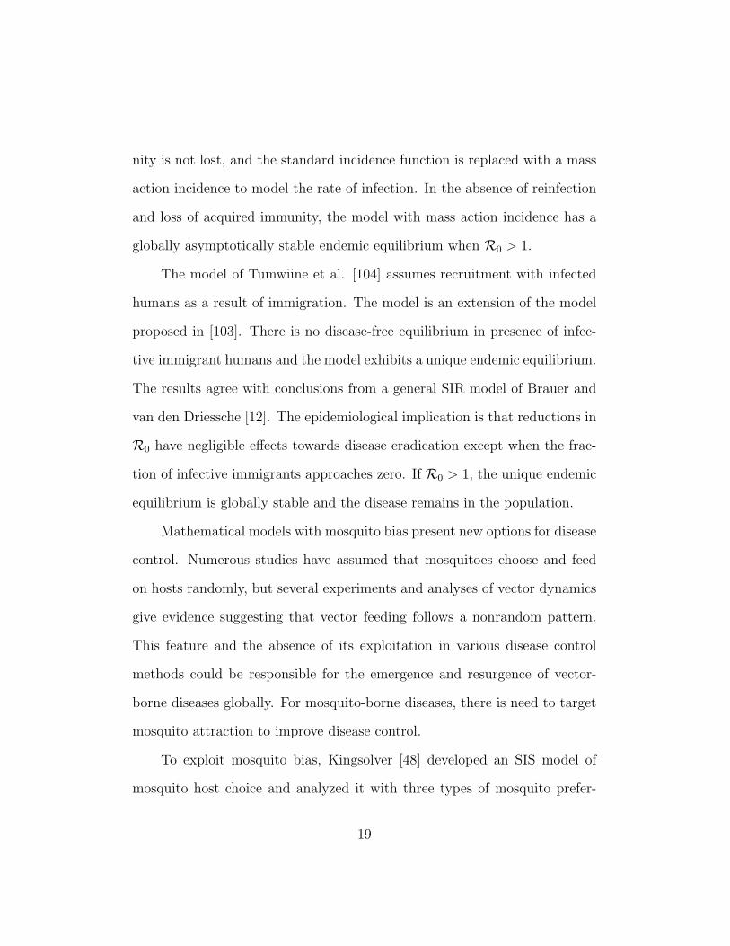
Several studies [2, 15, 22, 40, 111, 112] suggest that people can acquire
protection against mosquito bites through regular use of insecticide-treated
bed nets (see Figure 1.3). On the other hand, it is challenging to control
mosquito-borne diseases using bed nets alone because bed nets are only used
for a fraction of each day. It is important to examine how combining bed-net
usage with other disease-control approaches affects disease spread.
Photo taken by Tjeerd Wiersma from Amsterdam, The Netherlands.
Figure 1.3: Bed net: Ceiling hung mosquito netting.
To influence mosquito bias requires a combination of disease control
strategies, such as artificial feeders, attractants, repellents and bed nets,
but the effectiveness of such a multifaceted approach has not been studied
previously using mathematical models. In this study, we examine the effect
of influencing mosquito bias on disease transmission and spread. To do this
6

we develop three mathematical models of malaria incorporating a controlled
attractiveness of hosts to mosquitoes. The models are analyzed to examine
the effect of artificial feeders, attractants, repellents, and bed nets on disease
transmission and spread. Throughout this study, and wherever applicable,
the following explanation is implied for simplicity.
Hosts and vectors carrying transmissible stages of malaria parasites
are referred to as being ‘infectious’, whereas uninfected individu-
als and carriers of non-transmissible stages are referred to as being
‘noninfectious’. Individuals who successfully recover with immunity
to the pathogen are referred to as being ‘recovered’.
Given below are the main objectives of this study.
OB1: To find out if artificial feeders affect disease spread, and if so, find out
if they are a viable control measure.
OB2: To assess how the relative attractiveness of infectious humans using
protective odorants affects disease transmission and spread.
OB3: To examine how the odorant-acquisition rate during the infectious stage
affects disease transmission and spread.
OB4: To assess the effect of bed nets on disease spread and find out if the
disease can be eliminated with bed nets alone.
OB5: To examine the combined effect of odorants and bed nets on disease
spread in the presence of artificial feeders.
7

The artificial-feeder model is studied to examine the effect of mosquito
feeders and protective odorants or repellents on disease transmission and
spread. Mosquito bias is modelled by a dependence of the relative biting
rates on the attractiveness of infectious hosts. We show that mosquito bias
has a significant (and nonlinear) effect on disease spread.
The artificial-feeder model is modified to study the case without the
feeders and where infected humans acquire protective odorants during the
infectious stage. The resulting mosquito-bias model assumes that infectious
humans are either odorant users or non-users. The odorants are acquired to
manipulate the attractiveness of the users. The model is analyzed to examine
the effect of the odorant-acquisition rate on disease spread. The effect of the
odorant on disease control is also discussed.
Our third model combines the use of artificial feeders and protective
odorants with the use of bed nets, where a fraction of the human population
accounts for bed-net users. People can use protective odorants or bed nets
to prevent mosquito bites. Thus, mosquito bias is modelled by a dependence
of the relative biting rates on bed-net usage. The resulting bed-net model
is used to examine how the use of odorants or mosquito repellents and bed
nets affects disease transmission and spread. The effect of mosquito feeders
on disease-control outcomes is also discussed.
Although the three models are designed with a specific focus on malaria
control, they are applicable to many vector-borne pathogens. The proposed
disease control strategies are applicable to all mosquito-borne diseases.
8

1.2 Epidemiological Background
Malaria is a vector-borne disease caused by protozoan parasites of the genus
Plasmodium. According to the World Health Organisation [111], malaria is
caused by five parasite species in humans: Plasmodium falciparum, P. vivax,
P. ovale, P. malariae and P. knowlesi. Of these, P. falciparum and P. vivax
are the most common with P. falciparum being the most dangerous. The
pathogens are transmitted from host to host by infected female Anopheles
mosquitoes, which bite mainly between dusk and dawn [94, 77, 109, 111, 112].
Blood is required by the female mosquito for the protein needed to produce
eggs [23, 109]. An uninfected mosquito can acquire the pathogen when biting
an infected host and infect a new host during a subsequent bite.
The symptoms of malaria in an infected human include bouts of fever
and anaemia. On average, the latent period is about ten days in humans
[68] and about 11 days in mosquitoes [20]. The presentation may include
headache, fever, shivering, joint pain, vomiting, haemolytic anaemia, jaun-
dice, haemoglobin in the urine, retinal damage, and convulsions [11, 20]. If
left untreated, malaria can lead to severe complications and death [112].
Malaria is a public health problem causing many deaths around the
world. Malaria-related deaths can be reduced through disease control. In
1998, the World Health Organization in conjunction with other main inter-
national health agencies launched the Roll Back Malaria Global Partnership
with the goal of halving the global burden of malaria by 2010. This was
9

done by supporting numerous anti-malarial activities and research efforts
which can be seen in [111], A.10 of Chitnis [20] and other relevant sources.
The methods used in controlling malaria include larval control, which is
the destruction of breeding sites to reduce the number of mosquitoes; indoor
residual spraying, which reduces mosquito longevity and fertility; prompt and
effective case management to quickly identify and treat malaria cases, and
insecticide-treated bed nets. Bed nets are used to reduce mosquito-human
contacts. Preventing mosquito-human contacts can lead to mosquitoes biting
alternative hosts or not biting at all.
Further, certain disease-control approaches are undergoing research and
development. These include insecticide-treated livestock, which involves
treating cattle and other livestock with insecticides; intermittent prophy-
lactic treatment, which involves administering antimalarial drugs at regular
intervals to reduce parasitemia load; intermittent prophylactic treatment in
pregnancy, intermittent prophylactic treatment for infants to reduce infant
mortality, and gametocytocidal drugs targeting the reproduction of para-
sites in humans to reduce human-to-mosquito disease transmission. There
are plans to develop transmission-blocking vaccines [70, 100] and genetically
manipulated insect vectors [24, 65] to control the disease.
Malaria is endemic and widespread in tropical and subtropical regions,
including much of sub-Saharan Africa, Asia, and the Americas. According
to the World Health Organization’s World Malaria Report 2013 [111], there
were around 207 million cases of malaria in 2012 killing around 627 thousand
10

people. Malaria mortality rates were reduced by about 42% globally within
the period 2000-2012. During the same period, malaria incidence declined by
25% around the world. The reductions result from improvements in vector
control interventions, diagnostic testing and treatment. This represents a
substantial progress towards the World Health Assembly target of reducing
malaria mortality rates by 75% by the year 2015 [111].
Malaria transmission still occurs in 97 countries, putting more than 3.4
billion people at risk of illness. Four out of ten people who die of malaria live
in the two highest burden countries: the Democratic Republic of the Congo
and Nigeria [112]. Challenges such as drug resistance [5, 50, 77, 111], infected
travellers [77, 104, 111, 112], mosquito bias [19, 48, 52], and debilitating
effects of the disease burden on economic growth [38, 110] make malaria
control increasingly difficult. More effective approaches are needed to stop
the spread of the disease.
1.3 Mathematics for Malaria control
Although there are historical records1 suggesting that malaria has been killing
humans for thousands of years, the study of malaria using mathematics did
not begin until the 20th century. In fact, according to the Roll Back Malaria
Partnership [84], mathematical modelling began influencing public health
policy in 1766 when Daniel Bernoulli published a model of smallpox. Ronald
1Ancient Chinese, Indian, Greek and Roman writings (see A.2 of Chitnis [20]).
11

Ross began the study of malaria using mathematics at the beginning of the
20th century. A study by Smith et al. [95] gives a historical account in
which we see that Ross published his first dynamic malaria model in 1908
and coined the phrase “a priori pathometry” to describe the scientific activity
of modelling transmission dynamics. As seen in the account [95], the field
“a priori pathometry”, or “constructive epidemiology” [89], is now widely
known as mathematical epidemiology.
Following Ross’ ideas relating mosquito flight distances and densities to
larval control [85, 86], mathematical tools can be used to develop or support
malaria control strategies. Ross invented the idea of a threshold condition
defining a critical density of mosquitoes below which the malaria parasite
would die out. The threshold condition implied that it was not necessary
to kill every mosquito to eradicate malaria. Because of his work, malaria
control and elimination efforts focused on larval control.
Lotka [59] and Waite [107] further developed the dynamic model [86]
leading to a single difference equation model
Xt+1 = β0Xt(1−Xt
N)− αhXt,
where N is the constant human population size; Xt is the number of infected
humans at time t; αh is the recovery rate of each infected human; β0 is
Ross’ vectorial capacity describing the potential intensity of transmission by
mosquitoes. Ross’ time step was one month within which a mosquito made
12
two bites to complete the transmission cycle, whereas Waite considered the
interval between bites. The different time steps led to different results. Ross
improved the model to remove the dependency on the time step, and in 1911
he published the famous differential equation model [88].
Mathematicians who contributed to what is called the Ross-Macdonald
Theory, played a big role in malaria control. The model by Kermack and
McKendrick [46] and its subsequent extensions, which led to developments
in mathematical modelling, facilitated developments in malaria modelling.
The authors study a mathematical theory of epidemics and set conditions
relating population densities to the outcome of the epidemic given a suscep-
tible population. There is a natural removal of infected individuals through
various stages and the epidemic vanishes before the susceptible population
is exhausted. These developments were applicable to diseases which spread
through an intermediate host. More contributions from the paper and its
extensions are widely discussed by Brauer [13] and Dietz [31].
In 1950, George Macdonald focused on the mathematical theory of
malaria transmission [95] and tested Ross’ theory with field data [60, 61].
The World Health Assembly voted in 1955 to eradicate malaria and this was
based largely on indoor residual spraying with DDT because the field trials
had demonstrated its effectiveness in interrupting malaria transmission [84].
Macdonald’s analysis explained that insecticides greatly reduced the number
of mosquitoes that would live long enough to survive sporogony and transmit
malaria [84].
13

Macdonald, Irwin and Dietz worked together to develop a model that
incorporated immunity acquired after reinfection. A function accounting
for superinfection was considered by Macdonald and Irwin, and this was
improved later by Dietz. The model was tested in the Garki project [30, 68]
and was able to qualitatively reproduce the age-specific patterns in malaria
prevalence. With equations similar to Ross’ first model, Macdonald’s ideas
further led to the formulation of the Ross-Macdonald model [63] which has
driven much of the recent malaria modelling. The model and its subsequent
extensions are available in many forms [3, 7, 95]. We notice that in 1982,
Aron and May [7] first wrote the Ross-Macdonald model as
x′h = m0p1βxm(1− xh)− αhxh,
x′m = βxh(1− xm)− µmxm,(1.1)
where xh is the fraction of infectious humans at time t; xm is the fraction
of infectious female mosquitoes at time t; β is the biting rate per female
mosquito; p1 is the probability a bite by an infected mosquito on a susceptible
human host leads to infection of the human; m0 is the ratio of the total female
mosquito population size to the total human population size; αh is the rate
at which each human recovers from infection; and µm is the death rate of
adult female mosquitoes.
Models of the form (1.1) are widely studied. They are known to admit
two kinds of equilibria: a disease-free equilibrium if xh = xm = 0, and an
endemic equilibrium if xh, xm 6= 0. As a tradition, analysis of the disease-free
14

equilibrium includes a derivation of the threshold condition. Ross’ threshold
condition was redefined by Macdonald to become the basic reproduction ratio
R0 for malaria [62]. R0 for malaria is the expected number of new infected
hosts as a result of introducing one infected host in a completely susceptible
population. For history of R0 and its usage, see Heesterbeek and Dietz
[41, 42]. Koella [49] studies a Ross-Macdonald model and gives an algebraic
derivation of R0 showing that its threshold value is unity. For the malaria
model (1.1), the derivation gives
R0 =m0p1β
2
αhµm.
R0 is a measure of transmission intensity. It defines the extent to which a
given disease threatens a susceptible population in absence of disease control
measures. The larger the value of R0 the more severe is the disease spread.
The disease dies out if R0 < 1 and spreads in the population if R0 > 1.
Epidemic models in general divide a population into compartments based
on the number in each disease-state: S for susceptible; E for latently infected;
I for infectious; and R for recovered individuals. Thus, models are SIS, SIR,
SIRS, or SEIRS, where S, E, I, and R denote the numbers of individuals in
each of these compartments. Figure 1.4 illustrates a mathematical model
with SEIRS for the human population and SEI for the female mosquitoes.
Our models are based on this framework with notations such as ShEhIhRh
for the humans and SmEmIm for the mosquitoes.
15

Figure 1.4: A schematic diagram of the dynamics for malaria transmission.Susceptible populations Sh and Sm can acquire malaria pathogens throughcontacts with infectious groups Im and Ih respectively.
Extensions and modifications of the Ross-Macdonald model exist with
changes in the number of population compartments. We notice that models
like (1.1) are SIS. They assume all infected mosquitoes are infectious and
ignore a transmission-delay due to the latent period. Aron and May [7]
consider a second version of the Ross-Macdonald model which is a delay
model with the delay to account for the latent period. In both models,
immunity to the disease is boosted as a result of reinfection. The immunity
boost acquired by repeated infection was further studied by Aron [8, 9, 10].
Models represented by Figure 1.4 assume that recovered humans become
susceptible when the acquired immunity is lost.
16
Hethcote [43] and Mandal et al. [64] review several models including
some extensions of the Ross-Macdonal model. Anderson and May [3, 4]
considered (1.1) with changes in its second equation. This led to the equation
x′m = p2βxh(1−xm)−µmxm, where p2 is the probability a bite by a susceptible
mosquito on an infected human host leads to infection of the mosquito. They
also revisited the delay model and compiled data relating to the latent period,
the rate of recovery for humans, the expected adult lifespan of mosquitoes and
malaria prevalence across age distributions for humans. The latent period
was seen to lower the long term prevalence of the disease. We consider the
latent period by including classes for the latently infected Eh and Em as
shown in Figure 1.4. The probability p2 is also considered.
Recent mathematical models of malaria incorporate recruitment to the
susceptible class and infectiousness of individuals in various forms with an
assumption that mosquitoes choose and bite hosts randomly. Cai et al. [16],
Chitnis [20], Chitnis et al. [21], Mukandavire et al. [73], Ngwa and Shu
[74], Niger and Gumel [75], Okosun et al. [78], Olaniyi and Obabiyi [79],
Tumwiine et al. [103, 104] and several others study malaria dynamics with
recruitment to the susceptible class to reflect population-change as a result
of birth and immigration. There is need to use mathematical models to find
out how nonrandom feeding by mosquitoes affects disease dynamics.
It is important to mention that the disease-induced death of infectious
individuals, which is ignored in numerous studies, has received attention in
some recent works. Studies with SIS models like (1.1) ignore the death to
17

simplify analysis. This can also be seen in Koella and Antia [50] where
deaths are balanced by births into the susceptible class and the disease-
induced death is ignored to simplify analysis of disease control options. In
some cases, such as [16, 20, 75, 78, 79], the additional death may facilitate a
backward bifurcation leading to subcritical endemic equilibria for R0 < 1.
Ngwa and Shu [74] proposed a compartmental model for malaria with
varying population size. The SEIRS model was later studied and analyzed
by Chitnis [20] in a Ph.D. dissertation. The density-dependent and density-
independent death rates assumed in [20] led to the existence of two disease-
free equilibria: one in absence of mosquitoes and another in presence of both
populations. A unique endemic equilibrium was confirmed. Two reasonable
sets of baseline values for the parameters in the model were compiled, for high
and for low transmission regions. The sets were used to compute sensitivity
indices of R0. It was found out that the mosquito biting rate was the most
sensitive parameter in both high and low transmission regions, making it a
possible target for control with bed nets.
The model of Niger and Gumel [75] extends some earlier models of
malaria by including multiple infected and recovered classes to account for
the effect of reinfection. A backward bifurcation arises due to reinfection or
the use of standard incidence, and this cannot be averted by interchanging
standard incidence with a mass action incidence. The backward bifurcation
region increases with decreasing average life span of mosquitoes. However,
the phenomenon can be averted if reinfection does not occur, acquired immu-
18
nity is not lost, and the standard incidence function is replaced with a mass
action incidence to model the rate of infection. In the absence of reinfection
and loss of acquired immunity, the model with mass action incidence has a
globally asymptotically stable endemic equilibrium when R0 > 1.
The model of Tumwiine et al. [104] assumes recruitment with infected
humans as a result of immigration. The model is an extension of the model
proposed in [103]. There is no disease-free equilibrium in presence of infec-
tive immigrant humans and the model exhibits a unique endemic equilibrium.
The results agree with conclusions from a general SIR model of Brauer and
van den Driessche [12]. The epidemiological implication is that reductions in
R0 have negligible effects towards disease eradication except when the frac-
tion of infective immigrants approaches zero. If R0 > 1, the unique endemic
equilibrium is globally stable and the disease remains in the population.
Mathematical models with mosquito bias present new options for disease
control. Numerous studies have assumed that mosquitoes choose and feed
on hosts randomly, but several experiments and analyses of vector dynamics
give evidence suggesting that vector feeding follows a nonrandom pattern.
This feature and the absence of its exploitation in various disease control
methods could be responsible for the emergence and resurgence of vector-
borne diseases globally. For mosquito-borne diseases, there is need to target
mosquito attraction to improve disease control.
To exploit mosquito bias, Kingsolver [48] developed an SIS model of
mosquito host choice and analyzed it with three types of mosquito prefer-
19
ence for infected hosts: consistent preference, increasing preference, and a
switching behaviour with preference depending on the relative abundance of
infected and uninfected hosts. Kingsolver followed the results of Edman et al.
[33] showing that nonrandom feeding is expressed at three stages: attraction
and penetration, probing and the location of blood, and blood intake. The
author [48] discussed several laboratory experiments suggesting that mosqui-
toes prefer infected hosts to ones that are not infected. Thus, nonrandom
feeding was incorporated in the model to study how such feeding behaviour
could alter the conditions for the existence, stability, and levels of infection
at equilibrium. The author suggested that a more detailed study was needed
to better understand the dynamics of malaria.
Mosquito bias can influence the impact of bed-net usage on disease
spread. Agusto et al. [2] and Buonomo [15] model bed nets by a mosquito-
human contact rate, which is a linearly decreasing function of bed-net usage.
The models [2, 15] ignore bites during the day, which implies that bed nets
are 100% effective at all times. The bed-net model in [15] assumes mosquito
bias, where the bias refers to the enhanced relative attractiveness of infec-
tious humans to mosquitoes. The model suggests that mosquito bias may
negatively affect disease control as bed-net usage increases.
Bed nets can be used with other approaches to influence disease-control
outcomes. According to Lengeler [56], bed-net usage reduced malaria cases
by 50%. Bed nets provide complete protection from mosquitoes, but they are
only used by a fraction of the human population for a fraction of each day.
20

Protection from mosquito bites can be acquired through regular use of bed
nets [22, 40, 111, 112]. It is important to mention that there are no previous
studies showing how the use of bed nets together with repellents [1, 69, 93]
or artificial feeders could affect disease transmission and spread.
1.4 Mathematical Background
1.4.1 Basic system properties
Consider an infectious-disease model with n population compartments X1,
X2, . . . , Xn presented as a system of nonlinear differential equations:
X ′1 = f1(X1, X2, . . . , Xn),
X ′2 = f2(X1, X2, . . . , Xn),
...
X ′n = f1(X1, X2, . . . , Xn).
Using vector notation, let X = (X1, X2, . . . , Xn). The above system can be
written as
X ′ = f(X), (1.2)
where f = (f1, ..., fn) : U → Rn is continuous on set U , that is, f ∈ C(U).
In this case U is an open subset of Rn.
Definition 1.4.1 ([81], A solution of a system). A function X is a solution
21

of System (1.2) on an interval T 3 0 if X is differentiable on T and if for
all t ∈ T , X ∈ U satisfying (1.2). Given X0 ∈ U , X is a solution of the
initial value problem
X ′ = f(X), X(0) = X0, (1.3)
on an interval T 3 0 if X(0) = X0 and X is a solution of (1.2) on the
interval T ; X(0) = X0 is then called an initial condition of System (1.2).
Definition 1.4.2 ([81], The flow of a system). Let φ(t,X0) denote the so-
lution of the initial value problem (1.3) defined on its maximal interval of
existence, T (X0), then for t ∈ T (X0), the set of mapping φt defined by
φt(X0) = φ(t,X0)
is called the flow of System (1.2); φt is also referred to as the flow of the
vector field f(X).
Definition 1.4.3 ([81], Invariant Set). A set D ⊂ U is called invariant with
respect to the flow φt if φt(D) ⊂ D for all t ∈ Rn. Further, D is called
positively invariant with respect to the flow φt if φt(D) ⊂ D for all t ≥ 0.
Theorem 1.4.1 ([81], The Fundamental Existence-Uniqueness Theorem).
Let U 3 X0 be an open subset of Rn and assume that f is continuously
differentiable on U , then there exists τ > 0 such that the initial value problem
(1.3) has a unique solution X on the interval [−τ, τ ].
22
Theorem 1.4.2 ([80], Theorem 2.2.2, Comparison Theorem). Let f(t, x) be
continuous in an open set U containing a point (τ0, x0), and suppose that the
initial value problem
z′(t) = f(t, z(t)), z(τ0) = x0,
has a maximal solution z = z(t) with domain τ0 ≤ t ≤ τ1. If x is any
differentiable function on [τ0, τ1] such that (t, x(t)) ∈ U for t ∈ [τ0, τ1] and
x′(t) ≤ f(t, x(t)), τ0 ≤ t ≤ τ1, x(τ0) ≤ x0, (1.4)
then
x(t) ≤ z(t), τ0 ≤ t ≤ τ1. (1.5)
Moreover, the result remains valid if ‘maximal’ is replaced by ‘minimal’ and
< is replaced by > in both (1.4) and (1.5).
Definition 1.4.4 ([108], Equilibrium solution). An equilibrium solution of
System (1.2) is a particular point X∗ ∈ Rn such that f(X∗) = 0.
Theorem 1.4.3 ([82], Descartes Theorem). The number of positive roots
(counted according to their multiplicity) of a polynomial Pn(x) with real co-
efficients is either equal to the number of sign alterations in the sequence of
its coefficients or is by an even number less.
23

Definition 1.4.5 ([108], Definition 1.2.1, Liapunov stability). An equilibrium
solution X∗ is said to be Liapunov stable if for ε > 0, there exists a δ =
δ(ε) > 0, such that, for any solution X(t,X0) of (1.3), ||X0 − X∗|| < δ
implies ||X −X∗|| < ε for t > 0. An equilibrium which is not stable is called
unstable. In this case || · || denotes a norm in Rn.
Definition 1.4.6 ([108], Definition 1.2.2, Asymptotic stability). An equilib-
rium solution X∗ is said to be asymptotically stable if it is Liapunov stable
and if there exists a constant δ > 0 such that ||X0 −X∗|| < δ implies
limt→∞||X −X∗|| = 0.
Definition 1.4.7 ([97], Basin of attraction). The basin of attraction of an
equilibrium solution X∗ is the set of initial conditions X0 such that X → X∗
as t→∞.
1.4.2 Stability analysis
The stability of an equilibrium solution tells whether small perturbations
that start away from the solution decay or grow larger with time. For an
equilibrium solution, stability analysis is done by linearising f(X) using the
Jacobian matrix evaluated at the solution.
Theorem 1.4.4 ([108], Theorem 1.2.5). Suppose all of the eigenvalues of
J(X∗) have negative real parts. Then the equilibrium solution X = X∗ of the
nonlinear vector field X ′ = f(X) is asymptotically stable.
24

From (1.3), the Jacobian matrix of f(X) is defined as
J =
∂f1
∂X1
∂f1
∂X2
· · · ∂f1
∂Xn∂f2
∂X1
∂f2
∂X2
· · · ∂f2
∂Xn...
.... . .
...
∂fn∂X1
∂fn∂X2
· · · ∂fn∂Xn
.
Let X0 denote a disease-free equilibrium solution of (1.3). It follows
that the disease-free equilibrium is locally asymptotically stable if all eigen-
values of J(X0) have negative real parts. If applicable, the decomposition
method of van den Driessche and Watmough [106] is equivalent to checking
the eigenvalues of the Jacobian and is always sufficient.
Following [106], (1.3) can be written in terms of new functions as
X ′ = f(X) = g(X)− v(X), (1.6)
with v(X) = v−(X)−v+(X), where g(X) is the rate at which new infections
come into the system; v+(X) is the rate of transfer of individuals into the
system by all other means; and v−(X) is the rate of transfer of individuals
out of the system. Sort the compartments so that X = (Xa, Xb), where Xa
is a vector of compartments with infected individuals and Xb corresponds
to compartments with uninfected individuals. Similarly, define f = (fa, fb)
with fa = ga − va and fb = gb − vb.
If System (1.3) admits a disease-free equilibrium X0 and the functions
25

in (1.6) satisfy Lemma 1 of [106], then J(X0) admits the partitions below.
J(X0) =∂f
∂X(X0) =
[∂g
∂X(X0)− ∂v
∂X(X0)
]=
F 0
0 0
− V 0
Va Vb
,where F and V are square matrices with entries from Xa. F is nonnegative,
V is nonsingular and all eigenvalues of Vb have positive real parts.
F =
[∂ga∂Xa
(X0)
], V =
[∂va∂Xa
(X0)
],
and we can see that J(X0) admits a submatrix Jaa(X0) of the structure
Jaa(X0) = F − V. (1.7)
The product FV −1 is called the model’s next generation matrix. It fol-
lows that all eigenvalues of J(X0) have negative real parts if all eigenvalues
of Jaa(X0) have negative real parts. According to [106], all eigenvalues of
Jaa(X0) have negative real parts if and only if ρ(FV −1) < 1, where ρ denotes
the spectral radius. We square ρ(FV −1) and define a reproduction number
Rc =(ρ(FV −1)
)2. (1.8)
We refer to Rc as the control reproduction number for (1.3) in the presence
of disease control methods. The square is introduced for Rc to be consistent
with Macdonald’s definition of the reproduction number [62]. (ρ(FV −1))2
is
26

used if the cycle of infection has two generations, whereas ρ(FV −1) applies
to the case with one generation. If the controls are absent, then Rc = R0.
Theorem 1.4.5 ([106], Theorem 2). Consider the disease transmission model
given by (1.6). If X0 is a disease-free equilibrium of the model, then it is lo-
cally asymptotically stable if ρ(FV −1) < 1, but unstable if ρ(FV −1) > 1.
By Theorem 1.4.5, the Rc-definition (1.8) can be used to claim the
local stability status of the disease-free equilibrium. In fact X0 is locally
asymptotically stable if Rc < 1 and unstable if Rc > 1.
1.4.3 Backward bifurcation
Although the Rc-condition tells that the disease dies out if Rc < 1 and grows
if Rc > 1, some models admit subcritical endemic equilibria for Rc < 1 and
a bistability arises whereby a stable endemic equilibrium co-exists with the
stable disease-free equilibrium. This is because of a backward bifurcation
[18, 97, 105, 106] at the critical value Rc = 1. It is important to find a
subcritical value, denotedR∗c , below which the stable disease-free equilibrium
exists alone in its neighbourhood. We do this using the centre manifold
theory of bifurcation analysis found in [18, 81, 106] and several other texts.
First, choose a bifurcation parameter, say c, whose critical value c1 sat-
isfies Rc = 1. The Jacobian J(X0) computed at the disease-free equilibrium
is recomputed with c = c1 giving J(X0, c1) whose eigenvalues have negative
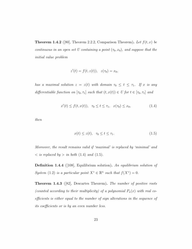
real parts except for a simple zero eigenvalue. Let u = (u1, u2, . . . , un) and
27
r = (r1, r2, . . . , rn) be the left and right eigenvectors respectively correspond-
ing to the simple zero eigenvalue. The eigenvectors satisfy
uJ(X0, c1) = J(X0, c1)r = 0.
The direction of the bifurcation at Rc = 1 is determined by the signs of the
bifurcation coefficients aB and bB computed as follows:
aB =n∑
k,i,j=1
ukrirj∂2fk
∂Xi∂Xj
(X0, c1),
bB =n∑
k,i=1
ukri∂2fk∂Xi∂c
(X0, c1).
If bB > 0 and aB > 0, then the model (1.6) exhibits a subcritical bifurcation
at Rc = 1. The direction of the bifurcation at Rc = 1 is backward, hence
backward bifurcation. The curve aB = 0 corresponds to Rc−R∗c = 0, giving
the stricter threshold below which the stable disease-free equilibrium exists
alone in its neighbourhood. At Rc = R∗c , the bifurcation is forward.
28

Chapter 2
A mathematical model of
Malaria control with artificial
feeders and protective odorants
2.1 Introduction
The transmission and spread of vector-borne diseases such as malaria, dengue,
West Nile virus and several others, is greatly influenced by vector behaviour.
Evidence suggests that mosquitoes do not choose hosts randomly [17, 52, 91,
93]. Carey and Carlson [17] suggest that a mosquito relies on its sense of
smell (olfaction) for locating food sources, hosts and egg-deposition sites. In
a study by Lacroix et al [52], the presence of gametocytes in malaria-infected
children increased mosquito attraction. In a controlled setting, Shirai et
29

al. [91] found that mosquitoes landed on people with Type O blood nearly
twice as often as those with Type A. This dependence of host-selection on
behaviour and cues is called mosquito bias.
Many mathematical models of vector-borne diseases incorporate several
features of population dynamics with the assumption that vectors bite hosts
randomly. For a survey of malaria models and their features, see recent works
by Cai et al. [16], Chitnis [20], Chitnis et al. [21], Mukandavire et al. [73],
Ngwa and Shu [74], Niger and Gumel [75], Okosun et al. [78], Olaniyi and
Obabiyi [79], Tumwiine et al. [104] and many others. The basic reproduction
number, which depends on disease-specific parameters, is used to analyze and
assess options for disease control without considering the effect of mosquito
bias on disease transmission and spread.
Following Kingsolver [48] and Lacroix et al [52] (reviewed in Chapter 1),
Chamchod and Britton [19] model mosquito bias towards infected humans
and measure mosquito attraction in terms of differing probabilities depending
on disease-status of the host. A mosquito arrives at a human host depending
on whether the human is infected or susceptible. The model is later studied
by Buonomo and Vargas-De-Leon [14] incorporating a disease induced death
rate. The studies [14, 19] suggest that the increased preference of humans
infected with malaria over uninfected individuals favours the high prevalence
of the parasites. This indicates the need to control mosquito bias.
From Chapter 1, mosquito bias can be influenced using odorants such
as mosquito attractants and repellents. A mosquito’s detector of a host can
30

be targeted using attractants (Potter [83] and Tauxe et al. [101]) to lure
mosquitoes away or into traps. Infected humans can use mosquito repellents
for protection against bites. Further, simplified devices–such as “glytube”
(Costa-da-Silva et al. [25]) and other simple membrane feeders–can be used
to artificially blood-feed mosquitoes.
We develop and analyze an artificial-feeder model to study the effect of
artificial feeders, mosquito attractants and repellents on disease transmission
and spread. Humans and mosquitoes with parasites in the infectious stage
are said to be infectious, whereas uninfected individuals and carriers of non-
transmissible stages are referred to as noninfectious. The model is used to
examine if artificial feeders affect disease spread, and if so, find out if the
feeders present a viable control measure. A disease control reproduction
number is derived to examine epidemiological conditions governing disease
spread. Analysis is done to assess the effect of repellents and attractants on
disease transmission and spread. The centre manifold theory of bifurcation
analysis is used to explore the existence of subcritical endemic equilibria and
bistability. We also examine the dependence of the direction of bifurcation on
the control parameters. Numerical simulations are done to support analytical
results which are also discussed.
31

2.2 The artificial-feeder model
2.2.1 Model formulation
The human population is divided into compartments depending on disease-
states Sh, Eh, Ih, Rh, where Sh is the number of susceptible humans, Eh is
the number of humans latently infected (not infectious), Ih is the number of
infectious humans, and Rh is the number of recovered humans with immunity
to the disease. Let Nh(t) be the total human population at time t; thus
Nh(t) = Sh(t) + Eh(t) + Ih(t) +Rh(t).
People are recruited to the susceptible class through birth at a constant
rate µhλh, which is assumed to be balanced by deaths, where µh is the per
capita natural death rate and λh is the constant human population in the
absence of the disease. Susceptible individuals may become infected through
contacts with infectious mosquitoes. It is assumed that only infectious mos-
quitoes can transmit infection to susceptible humans through bites. Infected
individuals go through a latent period, during which they do not transmit in-
fection. They progress from the latent stage to the infectious stage at the rate
γh. Infectious individuals recover at the rate αh with temporary immunity
to the disease or leave the population through an additional disease-induced
death rate, δh. Recovered humans lose the immunity and return to the sus-
ceptible class at the rate ρh.
32

Let Nm be the total mosquito population with three compartments
where Sm is the number of susceptible mosquitoes, Em is the number of
latently infected mosquitoes, and Im is the number of infectious mosquitoes.
At time t,
Nm(t) = Sm(t) + Em(t) + Im(t).
Mosquitoes enter the susceptible class through birth at a constant rate
µmλm, which is assumed to be balanced by deaths, where µm is the per capita
natural death rate and λm is the constant mosquito population in the absence
of the disease. It is probable that the parasite enters the mosquito through
biting an infectious human. It is assumed that only infectious humans can
transmit infection to susceptible mosquitoes through bites. Infected mosqui-
toes go through a latent period, during which they do not transmit infection.
Mosquitoes progress from the latent stage to the infectious stage at the rate
γm, and remain infectious for life. It is not clear if there are disease-induced
deaths among infectious mosquitoes. We assume that mosquitoes leave the
population through natural death.
From Smallegange et al. [93], malaria-infected mosquitoes express in-
creased attraction to human odour. Let β1 be the increased biting rate of
an infected mosquito and β2 denote the average biting rate of a susceptible
mosquito, where β1 ≥ β2. A mosquito approaches the vicinity of a host, but
this does not always translate into biting. In the presence of artificial feeders,
mosquito attraction to the feeder depends on the lure.
33

The formulation of the incidence function follows the conservation law,
that is, the total number of bites made by mosquitoes balances those received
by the hosts. Let Na be the number of feeders. Let ci, i = 1, 2, 3 be the
probability of a mosquito biting a noninfectious human, an infectious human
or an artificial feeder, respectively, given an encounter with such a host. In
this case, the distribution of bites depends on the probabilities ci. Given an
encounter rate θ (per day), a mosquito is likely to bite
θ(c1(Sh + Eh +Rh) + c2Ih + c3Na)
hosts per day. The probability a host bitten by a mosquito is a susceptible
human isc1Sh
(c1(Sh + Eh +Rh) + c2Ih + c3Na). Similarly, the probability a host
bitten is an infectious human isc2Ih
(c1(Sh + Eh +Rh) + c2Ih + c3Na).
The daily number of potentially infectious bites from mosquitoes is β1Im.
Let p1 be the probability a bite by an infectious mosquito on a susceptible hu-
man leads to infection of the human. Thus,c1p1β1ShIm
c1(Sh + Eh +Rh) + c2Ih + c3Na
is the incidence of new human infections. The daily number of bites from
susceptible mosquitoes is β2Sm. Let p2 be the probability a bite by a sus-
ceptible mosquito on an infectious human leads to infection of the mosquito.
The incidence of new mosquito infections isc2p2β2SmIh
c1(Sh + Eh +Rh) + c2Ih + c3Na
.
We introduce the following parameters to simplify the incidence terms.
βh = p1β1; βm = p2β2; c =c2c1
; A =c3c1Na. (2.1)
34

It is clear that if we set β1 = β2 = β, we can compensate for the actual
differences between β1 and β2 by choosing appropriate values for p1 and p2.
With the above description, our mathematical model consists of the
following system of differential equations.
S ′h = µh(λh − Sh)−βhShIm
Sh + Eh + cIh +Rh + A+ ρhRh,
S ′m = µm(λm − Sm)− cβmSmIhSh + Eh + cIh +Rh + A
,
E ′h =βhShIm
Sh + Eh + cIh +Rh + A− (γh + µh)Eh,
E ′m =cβmSmIh
Sh + Eh + cIh +Rh + A− (γm + µm)Em,
I ′h = γhEh − (αh + µh + δh)Ih,
I ′m = γmEm − µmIm,
R′h = αhIh − (ρh + µh)Rh.
(2.2)
Using vector notationX = (Sh, Sm, Eh, Em, Ih, Im, Rh), System (2.2) can
be studied as an initial value problem X ′ = f(X) with nonnegative initial
data X0, where X0 = X(0) = (Sh0, Sm0, Eh0, Em0, Ih0, Im0, Rh0).
The malaria model (2.2) is based on the following set of assumptions.
A1: There is a constant recruitment to the susceptible human population
as a result of birth, which is balanced by natural deaths.
A2: There is a constant recruitment to the susceptible mosquito population
as a result of birth, which is balanced by natural deaths.
35
A3: Transmission takes place only from infectious mosquitoes to susceptible
humans and from infectious humans to susceptible mosquitoes.
A4: Infected mosquitoes do not live long enough to recover from infection.
A5: Recovered humans have full immunity to the disease for a few years
after which the individuals become susceptible.
A6: Artificial feeders do not harbour or preserve disease parasites.
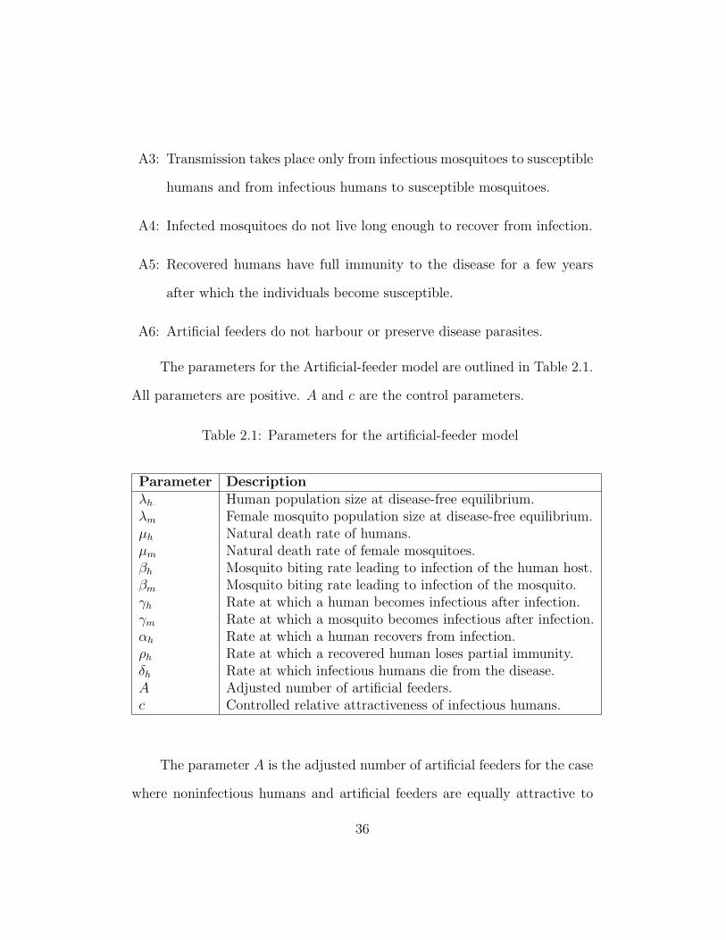
The parameters for the Artificial-feeder model are outlined in Table 2.1.
All parameters are positive. A and c are the control parameters.
Table 2.1: Parameters for the artificial-feeder model
Parameter Descriptionλh Human population size at disease-free equilibrium.λm Female mosquito population size at disease-free equilibrium.µh Natural death rate of humans.µm Natural death rate of female mosquitoes.βh Mosquito biting rate leading to infection of the human host.βm Mosquito biting rate leading to infection of the mosquito.γh Rate at which a human becomes infectious after infection.γm Rate at which a mosquito becomes infectious after infection.αh Rate at which a human recovers from infection.ρh Rate at which a recovered human loses partial immunity.δh Rate at which infectious humans die from the disease.A Adjusted number of artificial feeders.c Controlled relative attractiveness of infectious humans.
The parameter A is the adjusted number of artificial feeders for the case
where noninfectious humans and artificial feeders are equally attractive to
36

mosquitoes. c is the controlled relative attractiveness of infectious humans to
mosquitoes. The attractiveness is measured relative to that of noninfectious
individuals. Previous mosquito-bias models [14, 19, 48] are SIS, hence they
assume bias to all infected humans, with c > 1. Based on experimental
studies [52], the bias is towards humans who can transmit the parasite, and
these belong to the infectious class of the SEIRS model such as System (2.2).
For this study, c takes the following cases.
c > 1 : A mosquito is more likely to bite an infected human in the infectious
stage than a noninfectious individual upon encounter.
c = 1 : A mosquito is equally likely to bite an infected human in the infec-
tious stage and a noninfectious individual upon encounter.
c < 1 : A mosquito is less likely to bite an infected human in the infectious
stage than a noninfectious individual upon encounter.
2.2.2 Well-posedness
A mathematical model is well-posed (in the sense of Hadamard), if a solution
exists, the solution is unique, and the solution depends continuously on initial
data. By the basic theory of ordinary differential equations (Theorem 1.4.1),
the right hand side of (2.2) is differentiable on R7, which implies that a
unique solution X exists for every initial condition in R7.
Further, the model is epidemiologically well-posed if the solution is
always positive and bounded given nonnegative initial data. Thus, there
37
exists a domain of attraction for all positive solutions. All solutions with
Eh = Em = Ih = Im = 0 exist in the Sh − Sm − Rh plane, which we refer to
as a disease-free plane.
The following theorems and proofs show that the malaria model (2.2)
is epidemiologically well-posed with a solution which is always positive and
bounded given nonnegative initial data.
Theorem 2.2.1. For Model (2.2), the disease-free plane is invariant. All
solutions starting with Eh = Em = Ih = Im = 0 remain in the disease-free
plane for all time t > 0 with Sh > 0, Sm > 0, and Rh ≥ 0.
Proof . With Eh = Em = Ih = Im = 0, System (2.2) gives
S ′h = µh(λh − Sh) + ρhRh, S′m = µm(λm − Sm), R′h = −(ρh + µh)Rh, and
E ′h = E ′m = I ′h = I ′m = 0. Solving these yields Eh = Em = Ih = Im = 0,
Sh = λh−Sh0e−µht−Rh0e−(ρh+µh)t > 0, Sm = λm+(Sm0−λm)e−µmt > 0, and
Rh = Rh0e−(ρh+µh)t ≥ 0. The solutions exist in the disease-free plane.
Theorem 2.2.2 (Positivity of solutions). Model (2.2) is mathematically and
epidemiologically well-posed with a unique solution. Given nonnegative initial
data X0, the solution X is positive for all time t ≥ 0.
Proof . Consider System (2.2) with X = (Sh, Sm, Eh, Em, Ih, Im, Rh).
Suppose X0 > 0 and that at least one component of X is negative at some
time t > 0. By continuity and differentiability of X, there must be some
time t0 such that X(t) > 0 ∀t ∈ [0, t0) and one or more components of X(t0)
are zero with nonpositive derivatives. By the equation for S ′h, if Sh(t0) = 0
38

and µhλh + ρhRh(t0) ≤ 0, then Rh(t0) < 0 and Rh must be zero somewhere
on (0, t0). Hence Sh(t0) > 0. By the equation for S ′m, if Sm(t0) = 0, then
S ′m(t0) = µmλm, S ′m(t0) > 0 and hence Sm(t0) > 0. If Rh(t0) = 0 with R′h(t0)
nonpositive, then Ih(t0) must be nonpositive. Similarly, if Ih(t0) = 0 and
I ′h(t0) ≤ 0, then Eh(t0) ≤ 0; if Eh(t0) = 0 and E ′h(t0) ≤ 0, then Im(t0) ≤ 0
because Sh(t0) > 0; if Im(t0) = 0 and I ′m(t0) ≤ 0, then Em(t0) ≤ 0; and if
Em(t0) = 0 with E ′m(t0) ≤ 0, then Ih(t0) ≤ 0 because Sm(t0) > 0. Hence,
if X(t) > 0 on [0, t0) and any component of X(t0) is zero, then it must be
that at t0, Eh, Em, Ih, Im = 0 with E ′h, E′m, I
′h, I′m = 0. From the invariance of
the disease-free set (Theorem 2.2.1) and the uniqueness of solutions, having
Eh, Em, Ih, Im = 0 at t0 implies that ∀t > 0, Eh, Em, Ih, Im = 0, Sh > 0, Sm >
0, and Rh ≥ 0, contradicting the supposition that X(t) > 0 ∀t ∈ [0, t0).
Theorem 2.2.3 (Boundedness of solutions). Model (2.2) is mathematically
and epidemiologically well-posed. The solution X is bounded given nonnega-
tive initial data X0.
Proof . By the definitions of Nh and Nm, and Equations (2.2),
N ′h = (Sh + Eh + Ih + Rh)′ = S ′h + E ′h + I ′h + R′h ≤ µhλh − µhNh; and
N ′m = (Sm + Em + Im)′ = S ′m + E ′m + I ′m = µmλm − µmNm.
By the Comparison Theorem (see Theorem 1.4.2), integration gives
Nh ≤ λh + (Nh0 − λh)e−µht,
Nm = λm + (Nm0 − λm)e−µmt,(2.3)
39

∀t ≥ 0, where Nh0 and Nm0 are initial values. By positivity, Nh and Nm are
bounded between 0 and the solutions of (2.3), hence so are all components
of X (by positivity of each component).
Corollary 2.2.4 (Domain of attraction). For Model (2.2) with nonnegative
initial data X0, there exists a domain attracting all solutions X ∈ R7+.
Proof . Let the domain be denoted by D. From Equations (2.3), as t→∞,
Nh ≤ λh and Nm = λm. Nh < λh and Nm < λm for all time if this holds at
any time. Hence D is positive invariant and attracts all solutions.
By Theorem 2.2.2, if Sh = 0, then S ′h > 0; if Sm = 0, then S ′m > 0;
if Eh = 0, then E ′h ≥ 0; if Em = 0, then E ′m ≥ 0; if Ih = 0, then I ′h ≥ 0;
if Im = 0, then I ′m ≥ 0; and if Rh = 0, then R′h ≥ 0. Thus, the solutions
are bounded below by 0. Theorem 2.2.3 guarantees that the solutions are
bounded above. Given X0 ∈ R7+, the components of X are always contained
in the bounded domain given as follows.
D =
X ∈ R7
+
∣∣∣∣∣∣∣∣∣∣∣∣∣∣∣∣
Sh > 0, Sm > 0,
Eh ≥ 0, Em ≥ 0,
Ih ≥ 0, Im ≥ 0, Rh ≥ 0
Sh + Eh + Ih +Rh ≤ λh
Sm + Em + Im = λm
.
Consequently, System (2.2) has no orbits leaving D and all solutions are
attracted to this domain.
40

2.3 Equilibria and their stability
2.3.1 Disease-free equilibrium
A constant solution to a system of equations is referred to as an equilibrium
solution. A disease-free equilibrium refers to the equilibrium that exists in
the absence of the disease. For System (2.2), the equilibrium solutions satisfy
the following equations:
µh(λh − Sh)−βhShIm
Sh + Eh + cIh +Rh + A+ ρhRh = 0, (2.4a)
µm(λm − Sm)− cβmSmIhSh + Eh + cIh +Rh + A
= 0, (2.4b)
βhShImSh + Eh + cIh +Rh + A
− (γh + µh)Eh = 0, (2.4c)
cβmSmIhSh + Eh + cIh +Rh + A
− (γm + µm)Em = 0, (2.4d)
γhEh − (αh + µh + δh)Ih = 0, (2.4e)
γmEm − µmIm = 0, (2.4f)
αhIh − (ρh + µh)Rh = 0. (2.4g)
Theorem 2.3.1 (Boundary equilibria). System (2.2) has a unique disease-
free equilibrium and no other equilibria on the boundary of D.
Proof . Consider Equations (2.4). Suppose X∗ is a nonnegative equilibrium
solution of (2.4). By Equation (2.4a), X∗ ≥ 0 ⇒ S∗h > 0. Similarly, (2.4b)
⇒ S∗m > 0, (2.4c) ⇒ E∗h ≥ 0, (2.4d) ⇒ E∗m ≥ 0, (2.4e) ⇒ I∗h ≥ 0, (2.4f)
⇒ I∗m ≥ 0, and (2.4g) ⇒ R∗h ≥ 0. In addition, if R∗h = 0, then I∗h = 0; if
41

I∗h = 0, then E∗h = 0; if E∗h = 0, then I∗m = 0; if I∗m = 0, then E∗m = 0; if
E∗m = 0, then I∗h = 0; and if I∗h = 0, then R∗h = 0. Thus, at equilibrium, if
any of Eh, Em, Ih, Im, Rh is zero, then Eh = Em = Ih = Im = Rh = 0, and
hence the solution is on the disease-free set. Setting Eh, Em, Ih, Im, Rh = 0
in equations (2.4a) and (2.4b) proves uniqueness.
Theorem 2.3.1 implies that if X∗ is an equilibrium solution of System
(2.2) in the boundary of D, then Eh = Em = Ih = Im = Rh = 0. Let X0
denote the disease-free equilibrium solution. It follows that
X0 = (λh, λm, 0, 0, 0, 0, 0).
Stability of an equilibrium solution is investigated using linearization of
the system at the equilibrium. By Theorem 1.4.4, X0 is locally asymptoti-
cally stable if all eigenvalues of the Jacobian matrix, evaluated at X0, have
negative real parts. Let Rc be the control reproduction number for System
(2.2). The following definition for Rc is used to describe the stability of X0.
Definition 2.3.1. For the malaria model (2.2), the control reproduction
number Rc is defined as
Rc =cβhβmλhλmγhγm
(λh + A)2(γh + µh)(αh + µh + δh)(γm + µm)µm. (2.5)
From the definition, Rc is a function of disease-specific parameters and
control parameters. βhλh and βmλm are the rates of infection, 1/(αh+µh+δh)
42

and 1/µm are the life expectancies, γh/(γh + µh) and γm/(γm + µm) are the
fractions of the populations that progress to the infectious stage, whereas
c/(λh + A)2 is the control factor. Thus, Rc is the expected number of new
infected hosts as a result of introducing one infected host in a completely
susceptible population in the presence of mosquito bias and artificial feeders.
Theorem 2.3.2. For System (2.2), the disease-free equilibrium is locally
asymptotically stable if Rc < 1 and unstable if Rc > 1.
Proof . Let J(X0) denote the Jacobian matrix at X0. It follows that J(X0)
has the block structure
J(X0) =
J11 J12 J13
0 J22 0
0 J32 −(ρh + µh)
,
with submatrices
J11 =
−µh 0
0 −µm
, J12 =
0 0 0 − βhλhλh + A
0 0 − cβmλmλh + A
0
,
J22 =
−γh − µh 0 0βhλhλh + A
0 −γm − µmcβmλmλh + A
0
γh 0 −αh − µh − δh 0
0 γm 0 −µm
,
43

J32 = [ 0 0 αh 0 ], and J13 = [ ρh 0 ]T .
By the block structure of J(X0), X0 is locally asymptotically stable if all
eigenvalues of J11 and J22 have negative real parts. This is obvious for J11.
Note that J22 arises from the linear subsystem involving the infected compart-
ments. Hence, we can apply the decomposition method of van den Driessche
and Watmough [106] to derive a threshold condition for stability involving
the control reproduction number for the system. By equation (1.7), the sub-
matrix J22 admits the partition J22 = F − V , with
F =
0 0 0βhλhλh + A
0 0cβmλmλh + A
0
0 0 0 0
0 0 0 0
,
and
V =
γh + µh 0 0 0
0 γm + µm 0 0
−γh 0 αh + µh + δh 0
0 −γm 0 µm
.
Let ρ(·) denote the spectral radius of a matrix. Following [106], all eigenvalues
of J22 have negative real parts iff ρ(FV −1) < 1. There are two generations in
the cycle of infection. Thus, we square ρ(FV −1) and define a reproduction
number Rc = (ρ(FV −1))2, yielding the formula (2.5). The conclusion of
44

the proof follows from the fact that ρ(FV −1) < 1 implies (ρ(FV −1))2 < 1
(Theorem 1.4.5).
The product FV −1 is called the model’s next generation matrix. The
spectral radius ρ(FV −1) is also referred to as the dominant eigenvalue of
the matrix. Squaring ρ(FV −1) gives the traditional reproduction number
for vector-host models (Macdonald [62]). Rc is a function of the the control
parameters. In the absence of the controls, Rc gives the basic reproduction
number, R0, which is independent of mosquito bias and artificial feeders. It
is computed from Rc by setting c = 1 and A = 0, which yields
R0 =βhβmλmγhγm
λh(γh + µh)(αh + µh + δh)(γm + µm)µm. (2.6)
R0 is the expected number of new infected hosts as a result of introducing
one infected host in a completely susceptible population in the absence of
mosquito bias and artificial feeders.
Equations (2.5) and (2.6) give the Rc-R0 relation:
Rc = R0cλ2
h
(λh + A)2. (2.7)
If Rc < 1, then each infected human produces, on average, less than one
new infected human over the course of their infectious period in the presence
of malaria control methods, and the disease cannot invade the population.
Conversely, if Rc > 1, then each infected human produces, on average, more
45

than one new infected human in the presence of malaria control methods and
the disease can invade the population.
Equation (2.7) shows that Rc increases linearly with c and decreases
with A. Reducing mosquito bias towards infectious hosts reduces the control
reproduction number. In addition, Rc is decreasing with the number of
artificial feeders, A. Therefore, Rc can be reduced by reducing vector bias
for infectious hosts or increasing the number of artificial feeders until Rc < 1.
If this condition is not achieved, then Rc ≥ 1 and the disease persists.
2.3.2 Endemic equilibria
For System (2.2), any equilibrium solution in the interior of D is referred to
as an endemic equilibrium. Let X∗ denote the endemic equilibrium solution
for System (2.2) with Sh = S∗h, Sm = S∗m, Eh = E∗h, Em = E∗m, Ih = I∗h,
Im = I∗m, and Rh = R∗h. Solve for E∗h, E∗m and R∗h directly from equations
(2.4e), (2.4f) and (2.4g), respectively, in terms of I∗h and I∗m.
E∗h =(αh + µh + δh)I
∗h
γh, E∗m =
µmI∗m
γm, R∗h =
αhI∗h
ρh + µh. (2.8)
Further, S∗h + E∗h + I∗h +R∗h = λh − δhI∗h/µh, and S∗m + E∗m + I∗m = λm.
It follows that
S∗h = λh − ηhI∗h and S∗m = λm −(γm + µm)I∗m
γm, (2.9)
46

where
ηh = 1 +δhµh
+αh + µh + δh
γh+
αhρh + µh
. (2.10)
Solve for I∗m in terms of I∗h from (2.4a) using (2.8) and (2.9) and obtain
I∗m =
(λh + A− (1 +δhµh− c)I∗h)(γh + µh)(αh + µh + δh)I
∗h
βhγh(λh − ηhI∗h). (2.11)
Solve for I∗m in terms of I∗h from (2.4b) using (2.8) and (2.9) and obtain
I∗m =cβmλmγmI
∗h
(γm + µm)[cβmI∗h + µm(λh + A− (1 +δhµh− c)I∗h)]
. (2.12)
Notice that (2.11) and (2.12) can be equated and solved to give I∗h = 0, for
the disease-free equilibrium, which is obtained by factoring out I∗h. For the
endemic equilibria, let g1 and g2 be functions of I∗h derived from equations
(2.11) and (2.12), respectively, by dividing the equations by I∗h, where I∗h 6= 0.
The following are the resulting simultaneous equations.
g1 =I∗mI∗h
=(λh + A− (ξ2 − c)I∗h)(γh + µh)(αh + µh + δh)
βhγh(λh − ηhI∗h),
g2 =I∗mI∗h
=cβmλmγm
(γm + µm)(µm(λh + A)− (µm + βm)(ξ1 − c)I∗h)),
where
ξ1 =µm
µm + βm
(1 +
δhµh
), and ξ2 =
(1 +
δhµh
). (2.13)
47
By inspection, ξ2 > ξ1, and g1 and g2 give rectangular hyperbolas whose
properties change as c passes ξ1 and ξ2. The endemic equilibria are positive
solutions satisfying g1 − g2 = 0. Later we show that both g1 and g2 have to
be positive for the endemic equilibria to exist. Equating g1 and g2 leads to a
quadratic equation. The equation is written by making use of the formulae
for Rc and R0 to give
q2I∗2h + q1I
∗h + q0 = 0, (2.14)
where
q2 = (µm + βm)(ξ1 − c)(ξ2 − c),
q1 = cµmηhλhR0 + (λh + A)[cβm + 2µm(c− ξ2)],
q0 = µm(λh + A)2(1−Rc).
The endemic equilibria satisfy Equation (2.14). The solutions,
I∗h =−q1 ±
√q21 − 4q2q0
2q2,
correspond to the endemic equilibria of System (2.2) if I∗h ∈ D. The number
of positive solutions depends on the signs of the coefficients q2, q1 and q0. By
expansion, q0 = µm((λh +A)2 − cR0λ2h), and it is obvious that the solutions
are nonlinear functions of the control parameters A and c. As a result, it is
not clear how c affects I∗h.
Given −q1/q2 > 0, there exists a critical value of c below which, or above
which, c gives two positive values of I∗h. Let the value be denoted by c∗; we
compute it from the discriminant. Thus, c∗ is the solution of the equation
48
q21−4q2q0 = 0, and the two positive solutions exist if c satisfies q2
1−4q2q0 > 0.
Theorem 2.3.3. System (2.2) has no endemic equilibria if c = 0.
Proof . c = 0⇒ Rc = 0 and Equation (2.14) gives
I∗2h − 2(λh + A)
(1 + δh/µh)I∗h +
(λh + A)2
(1 + δh/µh)2= 0.
The result is a perfect square with I∗h = (λh +A)/(1 + δh/µh) > (λh +A)/ηh.
Consequently, equation (2.9) gives S∗h < 0, which nullifies the solution.
Although the quadratic equation (2.14) has two positive solutions for
c = 0 (or as c→ 0), the solutions are neither in D nor positive. By definition,
endemic equilibria have all components positive. All solutions that do not
satisfy this criterion are void, giving no corresponding endemic equilibria.
Thus, c∗ is the minimum value of c that gives two positive solutions. It
is still not clear if the two positive solutions exist for all c ≥ c∗. We study
the properties of g1 and g2 to examine how increasing c affects the number
of endemic equilibrium solutions. For the endemic equilibria, I∗h, I∗m > 0,
which implies that I∗m/I∗h > 0, hence g1, g2 > 0. Further, the denominator of
g1 must be positive, since it is βhγhS∗h, with S∗h from (2.9). Also, g1 and g2
must both be positive, hence the numerator of g1 and the denominator of g2
must be positive. Furthermore, S∗h > 0 ⇒ I∗h < λh/ηh. Thus, I∗h must be in
the interval (0, λh/ηh). For 0 ≤ c < ξ1, both the vertical and the horizontal
asymptotes of g1 are positive; the vertical asymptote of g2 is positive; and
49

the horizontal asymptote of g2 is at zero. In the positive quadrant with
0 < I∗h < λh/ηh, g1 and g2 intersect once or twice or never intersect.
For ξ1 ≤ c < ξ2, both the vertical and the horizontal asymptotes of
g1 are positive; and either g2 is a horizontal line or a rectangular hyperbola
with a negative vertical asymptote and a horizontal asymptote at zero. In
the positive quadrant with 0 < I∗h < λh/ηh, the functions intersect only once
or never intersect.
For ξ2 ≤ c <∞, the vertical asymptote of g1 is positive; the horizontal
asymptote of g1 is nonpositive; the vertical asymptote of g2 is negative; and
the horizontal asymptote of g2 is at zero. In the positive quadrant with
0 < I∗h < λh/ηh, the functions intersect only once or never intersect.
Thus, System (2.2) has two or no endemic equilibria or exactly one
endemic equilibrium for 0 ≤ c < ξ1, and the system has exactly one endemic
equilibrium or no endemic equilibria for ξ1 ≤ c < ∞. It is now clear that
c∗ < ξ1, and there must exist a minimum value of c for which the system
has exactly one endemic equilibrium. Let the value be denoted by c1. It is
clear that c∗ ≤ c1 < ξ1. In the special case if c∗ = c1, then the system has no
endemic equilibria (below c1) or exactly one endemic equilibrium (above c1).
By inspecting the quadratic equation (2.14), we conjecture on the existence
of endemic equilibria for the system.
Definition 2.3.2. Let c1 be a value of c satisfying Rc = 1. For System (2.2),
c1 =1
R0
(1 +
A
λh
)2
. (2.15)
50

Since Rc < 1⇔ c < c1 and Rc > 1⇔ c > c1, we conjecture using c1.
Conjecture 2.3.4. Let c1 be a value of c satisfying Rc = 1. For System
(2.2), there exists a subcritical value c∗ ≤ c1 such that,
(i) if 0 ≤ c < c∗, then the system has no endemic equilibria;
(ii) if c∗ < c < c1, then the system has two endemic equilibria; and
(iii) if c1 ≤ c <∞, then the system has exactly one endemic equilibrium.
In the special case if c∗ = c1, then there are no endemic equilibria for c < c1
and there is exactly one endemic equilibrium for c ≥ c1.
From the stability analysis of the disease-free equilibrium, the disease
can invade the population if c > c1. Conjecture 2.3.4 can be extended by
suggesting that the system (2.2) has exactly one endemic equilibrium which
is globally stable if Rc > 1. This leads to the following conjecture on the
stability of the endemic equilibrium.
Conjecture 2.3.5 (Stability of the endemic equilibrium). Let c1 be a value
of c satisfying Rc = 1. If c > c1, then the endemic equilibrium of System
(2.2) is globally asymptotically stable.
Conjectures 2.3.4 and 2.3.5 claim that if the system has exactly one
endemic equilibrium in addition to the disease-free equilibrium, then the
disease-free equilibrium is unstable and the endemic equilibrium is globally
stable for c > c1, that is, if Rc > 1. Analytic-global stability results are
51

not available for SEIRS vector-bias models. For the SIS vector-bias model
of Buonomo and Vargas-De-Leon [14], the geometric method due to Li and
Muldowney [57] is used to show that the endemic equilibrium is globally
asymptomatically stable in the interior of the domain of attraction if R0 > 1.
For vector-borne diseases with bilinear incidence terms, Lashari and Zaman
[54], Xiao [113] and Yang et al. [114] analyzed global stability for SEIR, SEI,
SI, and SIR models in which it is concluded that the endemic equilibrium is
globally stable if R0 > 1. Later we use numerical simulations to illustrate
the stability properties of the equilibria.
2.3.3 Bifurcation analysis
Several studies [16, 20, 75, 78, 79] show that the disease-induced death rate
δh facilitates a backward bifurcation by which at least two endemic equilibria
exist for Rc < 1. Later, we examine if the same effect of δh applies to System
(2.2). Conjecture 2.3.4 states that the system admits two endemic equilibria
if c∗ < c < c1. Since the disease-free equilibrium is stable for 0 ≤ c < c1
(Theorem 2.3.2), a bistability may arise as a result of one of the two endemic
equilibria being stable for c∗ < c < c1. This means that, with c∗ < c1,
reducing c below c1 may not necessarily guarantee disease eradication.
There exists exactly one endemic equilibrium for c ≥ c1, and c = c1
gives Rc = 1, which is a bifurcation point. The bifurcation point is when the
Jacobian of the system, evaluated at the equilibrium solution, has a simple
eigenvalue with zero real part. We examine the bifurcation and find out if
52
the direction of the bifurcation is forward or backward, and if the direction
really depends on any of the control parameters A and c or δh. A backward
bifurcation at c = c1 refers to the slope at the bifurcation point, and implies
that subcritical endemic equilibria may coexist with the stable disease-free
equilibrium if c < c1. In the following calculations, we use the centre manifold
theory of bifurcation analysis (discussed in [18, 81, 105, 106]) to show that a
subcritical bifurcation exists for some values of A and c or δh.
Let c be the bifurcation parameter. At the bifurcation point, set c = c1,
which is given in (2.15). Let J(X0, c1) be the Jacobian matrix computed
at the disease-free equilibrium X0, where c1 is the bifurcation value. The
eigenvalues of J(X0, c1) have negative real parts except for the simple zero
eigenvalue. Let u = (u1, u2, . . . , u7) and r = (r1, r2, . . . , r7) be the left and
right eigenvectors respectively corresponding to the simple zero eigenvalue,
that is, uJ(X0, c1) = J(X0, c1)r = 0.
Solving for u and r in terms of u3 and r3 gives
r1 = − [(γh + µh)(αh + µh + δh)(ρh + µh)− γhαhρh]r3(αh + µh + δh)(ρh + µh)µh
,
r2 =(λh + A)(γh + µh)(γm + µm)r3
βhγmλh,
u1 = 0, u2 = 0, u7 = 0, u4 =βhγmλhu3
(λh + A)(γm + µm)µm, u5 =
(γh + µh)u3
γh,
u6 =βhλhu3
(λh + A)µm, r4 =
(λh + A)(γh + µh)µmr3βhγmλh
, r5 =γhr3
(αh + µh + δh),
r6 =(γh + µh)(λh + A)r3
βhλh, and r7 =
αhγhr3(ρh + µh)(αh + µh + δh)
.
53
Evaluate second-order partial derivatives of the system at (X0, c1) and
use them to compute the bifurcation coefficients aB and bB given by
aB =7∑
k,i,j=1
ukrirj∂2fk
∂Xi∂Xj
(X0, c1),
bB =7∑
k,i=1
ukri∂2fk∂Xi∂c
(X0, c1).
The second-order partial derivatives of f5, f6 and f7 give zeros when evaluated
at (X0, c1), and the products with u1, u2 and u7 vanish because u1, u2, u7 = 0.
Further, it is important to note that
∂2fk∂Xi∂X4
= 0 : 1 ≤ k, i ≤ 7.
The surviving components of the calculations are given below:
∂2f3
∂X1∂X6
=∂2f3
∂X6∂X1
=βhA
(λh + A)2;
∂2f3
∂X3∂X6
=∂2f3
∂X6∂X3
=∂2f3
∂X6∂X7
=∂2f3
∂X7∂X6
= − βhλh(λh + A)2
;
∂2f3
∂X5∂X6
=∂2f3
∂X6∂X5
= −c∗ βhλh(λh + A)2
;
∂2f4
∂X1∂X5
=∂2f4
∂X5∂X1
=∂2f4
∂X5∂X3
=∂2f4
∂X3∂X5
= −c∗2 βmλm(λh + A)2
;
∂2f4
∂X5∂X7
=∂2f4
∂X7∂X5
= −c∗2 βmλm(λh + A)2
;
54

∂2f4
∂X2∂X5
=∂2f4
∂X5∂X2
= c∗2βm
λh + A;
∂2f4
∂X5∂X5
= −2c∗2βmλm
(λh + A)2.
The partial derivatives of the Jacobian with respect to c vanish except for
∂2f2
∂X5∂c= − βmλm
λh + A; and
∂2f4
∂X5∂c=
βmλmλh + A
.
Computing aB and bB with u3 = r3 = 1 gives
aB = λ2h(−(A/λh)
2 − 2(A/λh) + η1(1− A/λh) + η0),
bB =βhβmγhγmλhλm
(λh + A)2(αh + µh + δh)(γm + µm)µm,
where
η1 =µmR0
2µm + βm
[(γh + µh)(αh + µh + δh)(ρh + µh)− γhαhρh
γhµh(ρh + µh)
],
η0 =2µmR0
2µm + βm
(1 +
δhµh
)− 1.
η1 > 0 by inspection. Since bB > 0, a backward bifurcation exists if aB > 0.
Given that c is the bifurcation parameter, consider aB as a function of A.
Notice that aB(A) is decreasing with A, and aB(0) = λ2h(η1 + η0). Further,
aB(0) is increasing with δh, which gives support to the aforementioned effect
of δh on backward bifurcation. If αh >> δh, thenR0 and η1 are approximately
independent of δh and the only dependence of aB on δh is through η0. It is
55

now easy to see the effect of A and δh on the direction of the bifurcation.
Solving aB = 0 gives
Amin =λh2
(−2− η1 +
√4 + 8η1 + η2
1 + 4η0
), (2.16)
which is the minimum value of A required for the switch from aB > 0 to
aB < 0. A large value of δh/µh gives a large η0, which leads to aB > 0, hence
δh facilitates a backward bifurcation. A > Amin gives aB < 0, which leads to
a forward bifurcation. Thus, given aB > 0, the direction of bifurcation can
be switched from backward to forward by increasing A beyond Amin.
2.4 Parameter values
The artificial-feeder model is studied with the following parameter values.
There are no special restrictions on the parameter values except that they
should be positive and reasonable for mosquito-borne pathogens. Thus, the
values presented below are selected from literature or randomly assigned for
numerical simulations and to illustrate theoretical results from this study.
Included is the source or description of how each parameter value is obtained.
λh : Human population size in the absence of the disease. Assume 20,000
people. Reasonable range: 0 < λh <∞.
λm : Female-mosquito population size in the absence of the disease. Assume
40,000 mosquitoes. Reasonable range: 0 < λm <∞.
56

µh : Natural death rate of humans. Let the life expectancy be 70 years or
70×365 days. This gives µh = 1/25550 = 0.00004 per day. Reasonable
range: 0.000001 < µh < 0.001.
µm : Natural death rate of female mosquitoes. Several values have been
compiled by Chitnis [20] from different sources. Life expectancy for
Anopheles gambiae is 15.4 days (Garrett-Jones and Shidrawi (1969)).
µm = 1/15.4 = 0.065 per day. Reasonable range: 0.001 < µm < 0.1.
βh : Mosquito biting rate leading to infection of the human (p1β). β is the
average biting rate of a mosquito, and p1 is the probability a bite by
an infected mosquito on a susceptible human leads to infection of the
human. β = 0.4 (Peters and Standfast (1960) in [20]). p1 ∈ [0.05, 0.13]
(Krafsur and Armstrong (1978) in [20]). Suppose p1 = 0.05. It follows
that βh = 0.02 per day. Reasonable range: 0.001 < βh < 0.2.
βm : Mosquito biting rate leading to infection of the mosquito (p2β). p2 is
the probability a bite by a susceptible mosquito on an infected human
leads to infection of the mosquito. With p2 = 0.48 (Boyd (1941) and
Nedelman (1984) in [20]), βm = 0.192 per day. Reasonable range:
0.005 < βm < 0.4.
γh : Rate at which a human becomes infectious after infection. Latent period
for P. falciparum is 9− 10 days in humans (Molineaux and Gramiccia
[68]). Using 10 days, γh = 1/10 = 0.10 per day. Reasonable range:
0.06 < γh < 0.2.
57

γm : Rate at which a mosquito becomes infectious after infection. Latent
period for P. falciparum is 11 days in mosquitoes (Baker (1966) in [20]).
γm = 1/11 = 0.09 per day. Reasonable range: 0.02 < γm < 0.4.
αh : Rate at which a human recovers from infection. Estimated recovery
period for each human with P. falciparum is 9.5 months [68]. Using 30
days for each month, αh = 1/(9.5× 30) = 0.0035 per day. Reasonable
range: 0.001 < αh < 0.02.
ρh : Rate at which a recovered human loses partial immunity. Use 5 years
for the duration of acquired immunity and 365 days for each year. Thus
ρh = 1/(5× 365) = 0.0005 per day. Reasonable range: 0 < ρh < 0.01.
δh : Rate at which infectious humans die from the disease. Assume 220
deaths per year per 1000 infected people. δh = 0.0006 per day. If
disease-induced deaths are ignored, then δh = 0 per day. Reasonable
range: 0 < δh < 0.001.
A : Adjusted number of artificial feeders depending on the attractiveness of
artificial feeders to mosquitoes relative to that of humans. This is a
control parameter with A ∈ [0,∞). Reasonable range: 0 < A <∞.
c : Relative attractiveness of infectious humans to mosquitoes. This is a
control parameter with c ∈ [0,∞). Reasonable range: 0 < c <∞.
58

2.5 Discussion of results
In this section, the theoretical results are discussed with supporting figures.
All numerical simulations are done using parameter values in Table 2.2. A
discussion of the values and range can be found in Section 2.4.
Table 2.2: Parameter values used for simulations
Parameter Value Range Sourceλh 20,000 people (0,∞) §2.4λm 40,000 mosquitoes (0,∞) §2.4µh 0.00004 per day (0, 0.001) §2.4µm 0.065 per day (0.001, 0.1) [20]βh 0.02 per day (0.001, 0.2) [20]βm 0.192 per day (0.005, 0.4) [20]γh 0.10 per day (0.06, 0.2) [68]γm 0.09 per day (0.02, 0.4) [20]αh 0.0035 per day (0.001, 0.02) [68]ρh 0.0005 per day (0, 0.01) [20]δh 0.0006 per day (0, 0.001) §2.4A 0−∞ (0,∞) §2.4c 0−∞ (0,∞) §2.4
From Equation (2.6), R0 is a constant derived from disease-specific pa-
rameters whereas from Equation (2.7), Rc depends on the control parameters
A and c. It is clear that Rc decreases with increasing A, but the reductions
in Rc are negligible if A is negligible compared with λh. Taking the limit
as A → ∞ gives Rc = 0. For disease eradication based on artificial feeders,
A should be increased to be comparable to λh for all endemic equilibria to
vanish. This effect is illustrated in Figure 2.1.
59

By Equation (2.7), Rc increases linearly with c. The number of positive
real roots admitted by (2.14) is 0 or 2 or 1, depending on A and c. For
disease eradication based on mosquito bias, c should be reduced to near zero
for all endemic equilibria to vanish. This effect is illustrated in Figure 2.1.
The dependence of Rc on the control parameters has an effect on the
number of endemic equilibria. A and c have a combined effect on the number
of endemic equilibria. Figure 2.1 is used to illustrate Conjecture 2.3.4 which
states that there are subcritical endemic equilibria at small values of c, given
A. For disease eradication based on the value of Rc, c should satisfy c < c∗
depending on A, which gives region 0 of Figure 2.1.
Figure 2.1: Bifurcations in the c-A plane. The solid curve is Rc = 1, whichgives c = c1, whereas the dashed curve is q2
1 = 4q2q0, giving c = c∗. Inaddition to the disease-free equilibrium, given A, the number of endemicequilibria can be 0 for c < c∗; 2 for c∗ < c < c1; or 1 for c ≥ c1.
60

Recall from Equation (2.1) that A is the number of feeders scaled by
the relative attraction of mosquitoes to feeders. Hence, increasing A means
increasing the number of feeders or increasing the attractiveness of the feeders
relative to humans.
Bifurcation analysis suggests that there exists a backward bifurcation
giving rise to two endemic equilibria depending on A, c or δh. Using c as the
bifurcation parameter, the analysis shows that the direction of bifurcation
can be backward or forward, depending on A and δh. This is illustrated in
Figure 2.2 with the curve of Amin from Equation (2.16). A > Amin gives
aB < 0, hence the bifurcation becomes forward.
Figure 2.2: Effect of A on subcritical bifurcation. The curve aB = 0 givesAmin. Given δh, the bifurcation is backward if aB > 0, which applies toA < Amin, and A > Amin gives aB < 0 and hence a forward bifurcation.
61

Conjecture 2.3.4 states that, given c∗ and c1, a backward bifurcation
exists for c∗ < c1. The analysis shows that a large value of δh/µh facilitates
a backward bifurcation with aB > 0. The properties of g1 and g2 show that
there is exactly one endemic equilibrium for c ≥ ξ1. The sign change in aB as
A increases implies that c∗ and c1 are two different values. Thus, the curve
aB = 0 should match the intersection of c∗ and c1. The curve of Figure 2.2
is the locus of the fold bifurcation of Figure 2.1 following the intersection of
the dashed (c∗) and solid (c1) curves in the figure. With c∗ = c1, there are no
endemic equilibria for c < c1 and there is exactly one endemic equilibrium for
c > c1. This gives support to Conjecture 2.3.4. Moreover, the monotonicity
of aB with A implies that Figure 2.1 is generic, which gives further support
to the conjecture. Since A = 0 gives aB > 0 for large δh/µh, two endemic
equilibria I∗h exist for c∗ ≤ c < c1 or region 2 of Figure 2.3.
Figure 2.3: Effect of c on I∗h with A negligible. aB > 0 for δh/µh large and Anegligible. Two endemic equilibria exist for c∗ ≤ c < c1 inside region 2.
62

As a consequence of Conjecture 2.3.4, if c∗ < c1, then there is a backward
bifurcation at c1 with large δh/µh and there are two endemic equilibria as
well as a bistability for c∗ ≤ c < c1 (region 2 of Figure 2.3). In Figure
2.4, the curve with δh = 0.0006 illustrates that the backward bifurcation is
pronounced with large δh/µh. In contrast, for δh/µh small, c∗ does not exist,
hence there is no region of bistability for c. As illustrated in Figure 2.2, the
backward bifurcation disappears as δh → 0. This is the reason why Figure
2.4 gives a forward bifurcation with δh = 0.
Figure 2.4: Effect of c on I∗h with δh negligible. Setting A = 500 givesA/λh small. With A small, there is a backward bifurcation for δh/µh large(δh = 0.0006) and a forward bifurcation for δh/µh negligible (δh = 0).
By Theorem 2.3.2, the disease-free equilibrium is stable for Rc < 1 and
unstable for Rc > 1. Figure 2.5 illustrates the result that the disease-free
equilibrium is stable for Rc < 1, that is, for c < c1. Conjecture 2.3.5 implies
63
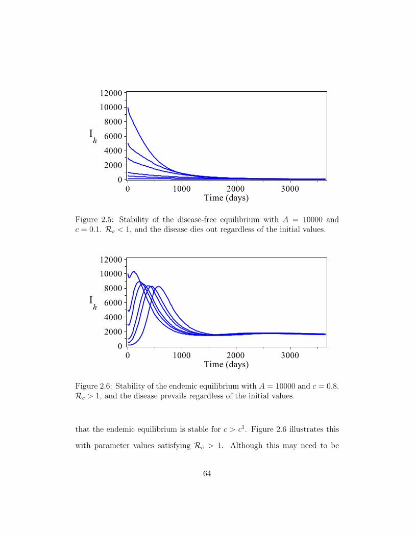
Figure 2.5: Stability of the disease-free equilibrium with A = 10000 andc = 0.1. Rc < 1, and the disease dies out regardless of the initial values.
Figure 2.6: Stability of the endemic equilibrium with A = 10000 and c = 0.8.Rc > 1, and the disease prevails regardless of the initial values.
that the endemic equilibrium is stable for c > c1. Figure 2.6 illustrates this
with parameter values satisfying Rc > 1. Although this may need to be
64

explored further, Figure 2.5 and Figure 2.6 illustrate the properties of the
equilibria in favour of Conjecture 2.3.5. Thus, it can be concluded that the
disease-free equilibrium is globally stable in region 0 of Figure 2.1, whereas
the endemic equilibrium is globally stable in region 1 of Figure 2.1.
2.6 Concluding remarks
The artificial-feeder model allows a critical analysis of disease-control options.
The objective was to examine the effect of artificial feeders and mosquito bias
on disease transmission and spread. c large and δh/µh large give a backward
bifurcation, whereas A/λh large facilitates a forward bifurcation. c small and
A/λh large give Rc small. Thus, the direction of bifurcation can be switched
from backward to forward by increasing A/λh or by decreasing c and δh/µh,
and disease spread can be stopped by increasing A/λh or by decreasing c.
Disease spread can be stopped by increasing A. Increasing A implies
increasing artificial feeders relative to humans and increasing the attractive-
ness of the feeders relative to uninfected humans. Potter [83] and Tauxe et
al. [101] suggest that mosquito attraction can be manipulated using attrac-
tants. In the artificial-feeder model, the attractiveness of the feeders can be
boosted using attractants. Thus, disease spread can be stopped by increasing
the number and attractiveness of artificial feeders relative to humans.
Disease spread can be stopped by decreasing c. From the bifurcation
analysis, disease eradication is not guaranteed even when mosquito bias c
65

is very small. Decreasing c implies decreasing the relative attractiveness of
infectious humans. There are subcritical endemic equilibria at a relatively
low attractiveness of infectious humans. Thus, the disease persists in the
populations for some values of c for which the control reproduction number
is less than unity. Our analysis shows that the endemic equilibria vanish by
increasing A/λh and by further decreasing c to near zero, which guarantees
disease eradication and global stability of the disease-free equilibrium.
There are no analytic global-stability results for the endemic equilibria.
Global stability of the endemic equilibrium has not been analyzed previously
for SEIRS models with mosquito bias. For SIS models, Buonomo and Vargas-
De-Leon [14] use the geometric method due to Li and Muldowney [57] and
show that the endemic equilibrium is globally stable if R0 > 1. Analysis is
available for single-population models (Korobeinikov [51]) and vector-borne
models without mosquito bias ([54], [113] and [114]) where it is concluded
that the endemic equilibrium is globally stable if R0 > 1. The models are
SEIR, SEI, SI or SIR. For [51, 54, 113], Lyapunov functions are used. System
(2.2) is SEIRS with mosquito bias. The analysis of the endemic equilibria
will be improved in future work to better understand the dynamics of the
disease with the proposed controls.
66
Chapter 3
A mosquito-bias model with
protective odorants for hosts in
the infectious stage
3.1 Introduction
Mosquito bias increases the speed of disease spread among humans. The
bias is expressed by the increased preference of infectious humans relative
to uninfected individuals (as discussed in Chapter 2). Mosquito bias can
be influenced by increasing or reducing mosquito attraction to hosts. From
Chapter 2, reducing attractiveness of infected humans to mosquitoes reduces
the disease control reproduction number. Thus, reducing the attractiveness
of infected humans in the infectious stage can slow or stop disease spread.
67

The attractiveness of hosts to vectors can be masked using protective
odorants or repellents to prevent infectious bites. In the artificial-feeder
model, the protective odorant is applied immediately at the onset of the
infectious period of infected humans. In this study we consider the case
where protective odorants are acquired by recruitment at the rate which can
be increased or decreased to improve the outcomes of disease control.
Repellents provide partial protection from bites, and the rate at which
the repellent is acquired may influence the effect of the repellent on disease
spread. We develop and analyze a mosquito-bias model to examine how the
recruitment rate for infected humans to use odorants affects disease spread.
The dependence of disease spread on the effectiveness of the odorant is also
discussed. Mosquito bias is modelled following the approach of Chapter 2.
3.2 The mosquito-bias model
3.2.1 Model formulation
The human population is divided into compartments Sh, Eh, Iu, Ip and Rh,
where Sh is the number of susceptible humans, Eh is the number of latently
infected humans (noninfectious), Iu is the number of unprotected-infectious
humans, Ip is the number of protected-infectious humans, and Rh is the
number of recovered humans. Let Nh(t) be the total human population at
time t; thus Nh(t) = Sh(t) + Eh(t) + Iu(t) + Ip(t) +Rh(t).
Humans are recruited to the susceptible class through birth at the rate
68

µhλh assumed to be balanced by deaths, where µh is the per capita natural
death rate and λh is the constant human population in the absence of the
disease. People may become infected through contacts with infectious mos-
quitoes. It is assumed that only infectious mosquitoes can transmit infection
to susceptible humans through bites. Infected humans go through a latent
period, during which they do not transmit infection, and they progress to
the infectious stage at the rate γh. Infectious individuals are recruited at the
rate νp (odorant-acquisition rate) to use protective odorants and recover at
the rate αh with temporary immunity to the disease or suffer disease-related
death at the rate δh. Recovered humans lose their immunity and return to
the susceptible class at the rate ρh.
Let Nm be the total vector-mosquito population with three compart-
ments where Sm is the number of susceptible mosquitoes, Em is the number
of latently infected mosquitoes (not infectious), and Im is the number of
infectious mosquitoes. Thus, at time t, Nm(t) = Sm(t) + Em(t) + Im(t).
Mosquitoes are assumed susceptible at birth. As with humans, mosqui-
toes are born at the rate µmλm balanced by deaths, where µm is the per
capita death rate and λm is the constant mosquito population in the absence
of the disease. It is probable that the parasite enters the mosquito through
biting an infectious human and we assume that only infectious humans can
transmit the infection to susceptible mosquitoes. Mosquitoes progress to the
infectious stage at the rate γm and remain infectious for life. Mosquitoes
leave the population through natural death.
69

Let β be the average biting rate of a mosquito. Following Chapter 2, let
ci, i = 1, 2, 3 be the probability of a mosquito biting a noninfectious host, a
protected infectious host or an unprotected infectious host, respectively, given
an encounter with such a host. It is assumed that every mosquito makes (on
average) β bites per day, regardless of the sequence in which they encounter
hosts. In this case, the distribution of bites depends on the probabilities ci.
The daily number of potentially infectious bites from mosquitoes is βIm.
Let p1 be the probability a bite by an infectious mosquito on a susceptible
host leads to infection of the host. Thus
c1p1βShImc1(Sh + Eh +Rh) + c2Ip + c3Iu
is the incidence of new human infections. Similarly, let p2 be the probability
a bite by a susceptible mosquito on an infectious host leads to infection of
the mosquito. Thus the incidence of new mosquito infections is
p2βSm(c2Ip + c3Iu)
c1(Sh + Eh +Rh) + c2Ip + c3Iu.
c3 > c2 if the odorant repels mosquitoes and c3 = c2 in the absence of the
protective odorant. Unlike in Chapter 2 where the protective odorant is
acquired by all infected humans at the onset of the infectious period, we
focus on the case where some infected humans do not acquire the repellent
and hence attract mosquitoes more than repellent-users do.
With the above description, the mosquito-bias model consists of the
70

following system of differential equations.
S ′h = µh(λh − Sh)−βhShIm
Sh + Eh + cIp + εIu +Rh
+ ρhRh,
S ′m = µm(λm − Sm)− βmSm(cIp + εIu)
Sh + Eh + cIp + εIu +Rh
,
E ′h =βhShIm
Sh + Eh + cIp + εIu +Rh
− (γh + µh)Eh,
E ′m =βmSm(cIp + εIu)
Sh + Eh + cIp + εIu +Rh
− (γm + µm)Em,
I ′u = γhEh − (αh + µh + δh)Iu − νpIu,
I ′p = νpIu − (αh + µh + δh)Ip,
I ′m = γmEm − µmIm,
R′h = αh(Ip + Iu)− (ρh + µh)Rh,
where
βh = p1β; βm = p2β; c =c2c1
; and ε =c3c1
(3.1)
to simplify the incidence terms. ε represents the natural mosquito-preference
of infectious humans over noninfectious individuals, thus ε > 1. c is the
controlled relative attractiveness of infectious humans who use the repellent.
In the absence of the protective repellent, c = ε
The above system can easily be written in a rescaled form. We scale
the number of individuals in each class by the constant species population.
This enables us to study proportions of the populations with respect to the
71
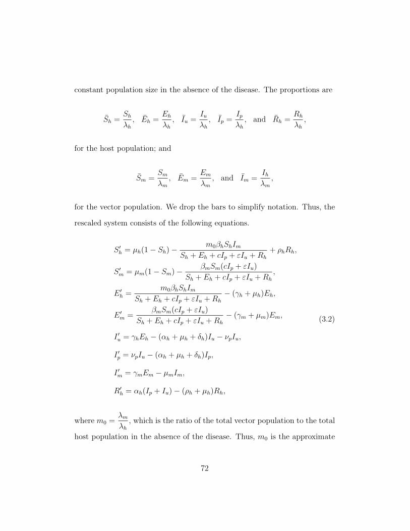
constant population size in the absence of the disease. The proportions are
Sh =Shλh, Eh =
Ehλh, Iu =
Iuλh, Ip =
Ipλh, and Rh =
Rh
λh,
for the host population; and
Sm =Smλm
, Em =Emλm
, and Im =Ihλm
,
for the vector population. We drop the bars to simplify notation. Thus, the
rescaled system consists of the following equations.
S ′h = µh(1− Sh)−m0βhShIm
Sh + Eh + cIp + εIu +Rh
+ ρhRh,
S ′m = µm(1− Sm)− βmSm(cIp + εIu)
Sh + Eh + cIp + εIu +Rh
,
E ′h =m0βhShIm
Sh + Eh + cIp + εIu +Rh
− (γh + µh)Eh,
E ′m =βmSm(cIp + εIu)
Sh + Eh + cIp + εIu +Rh
− (γm + µm)Em,
I ′u = γhEh − (αh + µh + δh)Iu − νpIu,
I ′p = νpIu − (αh + µh + δh)Ip,
I ′m = γmEm − µmIm,
R′h = αh(Ip + Iu)− (ρh + µh)Rh,
(3.2)
where m0 =λmλh
, which is the ratio of the total vector population to the total
host population in the absence of the disease. Thus, m0 is the approximate
72

number of female mosquitoes per person in the absence of the disease.
The malaria model (3.2) is based on the assumptions A1-A5 of the
artificial-feeder model discussed in Chapter 2.
Using vector notation, let X = (Sh, Sm, Eh, Em, Iu, Ip, Im, Rh) denote a
solution of System (3.2) and X0 = (Sh0, Sm0, Eh0, Em0, Iu0, Ip0, Im0, Rh0) be
the nonnegative initial data, where X0 = X(0).
The parameters for the mosquito-bias model are outlined in Table 3.1.
All parameters are positive. c and νp are the control parameters.
Table 3.1: Parameters for the mosquito-bias model
Parameter Descriptionµh Natural death rate of humans.µm Natural death rate of female mosquitoes.βh Mosquito biting rate leading to infection of the human host.βm Mosquito biting rate leading to infection of the mosquito.γh Rate at which a human becomes infectious after infection.γm Rate at which a mosquito becomes infectious after infection.αh Rate at which a human recovers from infection.ρh Rate at which a recovered human loses partial immunity.δh Malaria-induced death rate of infectious humans.m0 Ratio of total mosquito population to human population.ε Natural relative attractiveness of infectious humans.c Controlled relative attractiveness of infectious humans.νp Recruitment rate for infectious humans to use odorants.
73

3.2.2 Well-posedness
Following similar approaches of Chapter 2, the right hand side of (3.2) is
differentiable on R8, which implies that a unique solution X exists for every
initial condition. The following theorems guarantee that System (3.2) is
mathematically and epidemiologically well-posed with a solution which is
always positive and bounded given nonnegative initial data.
Theorem 3.2.1. For Model (3.2), the disease-free plane is invariant. All
solutions starting with Eh = Em = Iu = Ip = Im = 0 remain in the disease-
free plane for all time t > 0 with Sh > 0, Sm > 0, and Rh ≥ 0.
Theorem 3.2.2 (Positivity of solutions). Model (3.2) is mathematically and
epidemiologically well-posed with a unique solution. Given nonnegative initial
data X0, the solution X is positive for all time t ≥ 0.
Theorem 3.2.3 (Boundedness of solutions). Model (3.2) is mathematically
and epidemiologically well-posed. The solution X is bounded given nonnega-
tive initial data X0.
Corollary 3.2.4 (Domain of attraction). For Model (3.2) with nonnegative
initial data X0, there exists a domain attracting all solutions X ∈ R8+.
Following a similar approach of Chapter 2, it can be shown that there
exists a domain of attraction such that for any trajectory that starts in the
domain, the solution X is always contained in the interior and boundary
of the domain. Let the domain of attraction be denoted by D. Since the
74

components of X are positive and bounded, we write
D =
X ∈ R8
+
∣∣∣∣∣∣∣∣∣∣∣∣∣
Sh > 0, Sm > 0, Eh ≥ 0, Em ≥ 0,
Iu ≥ 0, Ip ≥ 0, Im ≥ 0, Rh ≥ 0
Sh + Eh + Iu + Ip +Rh ≤ 1
Sm + Em + Im = 1
.
3.3 Equilibria and their stability
3.3.1 Disease-free equilibrium
As seen in Chapter 2, a constant solution to a system of equations is referred
to as an equilibrium solution. The Equilibrium solutions of System (3.2)
satisfy the following equations.
µh(1− Sh)−m0βhShIm
Sh + Eh + εIu + cIp +Rh
+ ρhRh = 0, (3.3a)
µm(1− Sm)− βmSm(εIu + cIp)
Sh + Eh + εIu + cIp +Rh
= 0, (3.3b)
m0βhShImSh + Eh + εIu + cIp +Rh
− (γh + µh)Eh = 0, (3.3c)
βmSm(εIu + cIp)
Sh + Eh + εIu + cIp +Rh
− (γm + µm)Em = 0, (3.3d)
γhEh − (αh + µh + δh)Iu − νpIu = 0, (3.3e)
νpIu − (αh + µh + δh)Ip = 0, (3.3f)
γmEm − µmIm = 0, (3.3g)
αh(Iu + Ip)− (ρh + µh)Rh = 0. (3.3h)
75

For a disease-free equilibrium, there is no disease and hence all components
corresponding to infected individuals are empty.
Theorem 3.3.1 (Boundary equilibria). System (3.2) has a unique disease-
free equilibrium and no other equilibria on the boundary of D.
This theorem is similar to Theorem 2.3.1. The domain D is positively
invariant and the equilibrium in the boundary is the only equilibrium of (3.2)
without the disease. By Theorem 3.2.2 and Equations (3.3), it is straight
forward that if any of Eh, Em, Iu, Ip, Im, Rh, is positive, then all components
of X are positive and the equilibrium is strictly positive. Let X0 denote the
disease-free equilibrium solution. It follows that
X0 = (1, 1, 0, 0, 0, 0, 0, 0).
Local stability analysis of X0 follows similar analyses in Chapter 2. Let Rc
denote the control reproduction number for System (3.2). Further, let
ωh = αh + µh + δh. (3.4)
ωh is the rate at which infected humans leave the infectious stage.
Definition 3.3.1. For the malaria model (3.2), the control reproduction
number Rc is defined as
Rc =m0βhβmγhγm(ωhε+ νpc)
(γh + µh)(ωh + νp)(γm + µm)ωhµm. (3.5)
76

Rc is the expected number of new infected hosts as a result of introducing
one infected host in a completely susceptible population in the presence of
disease control methods.
Theorem 3.3.2. For System (3.2), the disease-free equilibrium is locally
asymptotically stable if Rc < 1 and unstable if Rc > 1.
Proof . Let J(X0) denote the Jacobian matrix at X0. The Jacobian matrix
has the block structure
J(X0) =
J11 J12 J13
0 F − V 0
0 J32 −(ρh + µh)
,
with
J11 =
−µh 0
0 −µm
, J12 =
0 0 0 0 −m0βh
0 0 −εβm −cβm 0
,
J13 =
ρh
0
, J32 =
0
0
αh
αh
0
T
, F =
0 0 0 0 m0βh
0 0 εβm cβm 0
0 0 0 0 0
0 0 0 0 0
0 0 0 0 0
,
77

and
V =
γh + µh 0 0 0 0
0 γm + µm 0 0 0
−γh 0 ωh + νp 0 0
0 0 −νp ωh 0
0 −γm 0 0 µm
,
where ωh = αh + µh + δh from Equation (3.4). X0 is locally asymptotically
stable if all eigenvalues of J(X0) have negative real parts (Theorem 1.4.4).
From the structure of J(X0), all eigenvalues of [F−V ] must have negative real
parts. By the decomposition method of van den Driessche and Watmough
[106], all eigenvalues of [F −V ] have negative real parts iff ρ(FV −1) < 1. We
set Rc = (ρ(FV −1))2, which yields Equation (3.5). The conclusion of the
proof follows from Theorem 1.4.5.
Rc is referred to as the control reproduction number for System (3.2).
The corresponding basic reproduction numberR0 accounts for disease spread
without protection, that is for νp = 0 and c = ε. It follows that
R0 =εm0βhβmγhγm
(γh + µh)(γm + µm)ωhµm. (3.6)
Equations (3.5) and (3.6) give
Rc = R0
ωh +c
ενp
ωh + νp
. (3.7)
78

For the malaria model (3.2), R0 is the expected number of new infected
hosts as a result of introducing one infected host in a completely susceptible
population in the absence of the protection.
From Equation (3.7), Rc increases linearly with c, whereas the effect
of νp depends on the ratio c/ε. Increasing νp decreases Rc if c < ε. If
Rc < 1, then each infected human produces, on average, less than one new
infected human over the course of their infectious period in the presence of the
protection, and the infection cannot grow. Conversely, if Rc > 1, then each
infected human produces, on average, more than one new infected human in
the presence of the protection and the disease can invade the population.
3.3.2 Endemic equilibria
For System (3.2), any equilibrium solution in the interior of D is referred to
as an endemic equilibrium. Let X∗ = (S∗h, S∗m, E
∗h, E
∗m, I
∗u, I
∗p , I
∗m, R
∗h) denote
the endemic equilibrium solution of System (3.2) satisfying Equations (3.3).
Solving Equations (3.3) in terms of I∗u and I∗m gives
S∗h = 1− ηpI∗u, E∗h =
(ωh + νp)I∗u
γh, I∗p =
νpI∗u
ωh,
R∗h =αh(ωh + νp)I
∗u
ωh(ρh + µh), S∗m = 1− (γm + µm)I∗m
γm, E∗m =
µmI∗m
γm,
(3.8)
where
ηp =(ωh + νp)[γh(ρh + µh)(µh + δh) + γhαhµh + (ρh + µh)ωhµh]
(ρh + µh)γhωhµh. (3.9)
79

We continue to solve for I∗u and I∗m and obtain the simultaneous equations
g1 =I∗mI∗u
=(γh + µh)(ωh + νp)(ωh − νp(ξ∗2 − c)I∗u)
m0βhγhωh(1− ηpI∗u),
g2 =I∗mI∗u
=βmγm(ωhε+ νpc)
(γm + µm)(µmωh − νp(µm + βm)(ξ∗1 − c)I∗u),
where
ξ∗1 =µm
µm + βm
(1 +
δhµh
)(1 +
ωhνp
)− ωhνpε,
and
ξ∗2 =
(1 +
δhµh
)(1 +
ωhνp
)− ωhνpε.
The functions g1 and g2 are obtained following the approach of Chapter 2.
Equating g1 and g2 leads to the quadratic equation
q2I∗2u + q1I
∗u + µmω
2h(1−Rc) = 0, (3.10)
where
q2 = ν2p(µm + βm)(ξ∗1 − c)(ξ∗2 − c),
q1 = ω2hµmηpRc − ωhνp[(µm + βm)(ξ∗1 − c) + µm(ξ∗2 − c)].
The positive solutions of (3.10) correspond to the endemic equilibria of
(3.2) if they are in the interior of D. By Equations (3.8), the solutions satisfy
0 ≤ I∗u < 1/ηp. The number of positive solutions depends on the signs of q2,
q1 and 1−Rc. ξ∗1 and ξ∗2 are two critical values of c giving q2 = 0 and exactly
80

one solution. To examine the existence of endemic equilibria for c from 0
to ∞, we use a similar approach of Chapter 2. Notice that g1 and g2 give
rectangular hyperbolas whose properties change as c passes ξ∗1 and ξ∗2 . The
hyperbolas intersect only once in the positive quadrant with 0 ≤ I∗u < 1/ηp
if c ≥ ξ∗1 . Since ξ∗2 > ξ∗1 , a deduction can be made leading to a conjecture on
the existence of two endemic equilibria. In fact, if 0 ≤ c < ξ∗1 , then System
(3.2) has two or no endemic equilibria or exactly one endemic equilibrium.
If ξ∗1 ≤ c < ∞, then the system has no endemic equilibria or exactly one
endemic equilibrium. Let c∗ be the positive solution of the equation
q21 − 4q2µmω
2h(1−Rc) = 0.
Given −q1/q2 > 0, Equation (3.10) has two positive real roots for c satisfying
q21 − 4q2µmω
2h(1−Rc) > 0.
Since q1, q2 and Rc increase with c, the inequality holds for c > c∗ if Rc < 1,
and if Rc = 1, then Equation (3.10) has exactly one root and the inequality
holds for a relatively higher value of c. It is now clear that for Rc < 1, there
are two positive roots for c > c∗ or one root for c >> c∗.
Definition 3.3.2. Let c1 be a value of c satisfying Rc = 1. For System (3.2),
c1 =ε
R0
(1− (R0 − 1)
ωhνp
). (3.11)
81
Since Rc < 1⇔ c < c1 and Rc > 1⇔ c > c1, we conjecture using c1.
Conjecture 3.3.3. Let c1 be a value of c satisfying Rc = 1. For System
(3.2), there exists a subcritical value c∗ ≤ c1 such that,
(i) if 0 ≤ c < c∗, then the system has no endemic equilibria;
(ii) if c∗ < c < c1, then the system has two endemic equilibria; and
(iii) if c1 ≤ c <∞, then the system has exactly one endemic equilibrium.
In the special case if c∗ = c1, then there are no endemic equilibria for c < c1
and there is exactly one endemic equilibrium for c ≥ c1.
The disease-free equilibrium is unstable if Rc > 1. Conjecture 3.3.3
implies that the malaria model (3.2) has exactly one endemic equilibrium
and an unstable disease-free equilibrium if Rc > 1. There are no analytic
global-stability results for the endemic equilibria of System (3.2). The control
parameters c and νp and ratio c/ε are still under investigation.
3.4 Results and discussion
Given below are the results of the model together with supporting figures.
All numerical simulations are done using parameter values in Table 3.2. A
discussion of the values and range can be found in Section 2.4.
Equation (3.7) shows that Rc increases linearly with c. Since protection
is a repellent, improved protection is modelled by decreasing c. Reducing the
82

Table 3.2: Parameter values used for simulations
Parameter Value Range Sourceµh 0.00004 per day (0, 0.001) §2.4µm 0.065 per day (0.001, 0.1) [20]βh 0.02 per day (0.001, 0.2) [20]βm 0.192 per day (0.005, 0.4) [20]γh 0.10 per day (0.06, 0.2) [68]γm 0.09 per day (0.02, 0.4) [20]αh 0.0035 per day (0.001, 0.02) [68]ρh 0.0005 per day (0, 0.01) [20]δh 0.0006 per day (0, 0.001) §2.4m0 2.0 mosquitoes per person (0, 10) §2.4ε 1.5 (1.0, 2.0)c 0− ε (0, ε) §2.4νp 0−∞ per day (0,∞)
relative attractiveness of infectious humans who use the repellent decreases
the disease control reproduction number. The ratio c/ε is the preference for
protected humans over unprotected individuals, given both are infectious.
For a mosquito repellent c/ε < 1, hence c < ε. Rc increases linearly with c
from R0ωh
ωh + νpto R0 as c increases from 0 to ε.
Further, Equation (3.7) shows that Rc increases or reduces nonlinearly
with νp, depending on c. Rc = R0 when νp = 0, and Rc = R0c
εas νp →∞.
Thus Rc is decreasing (hyperbolically) with νp if c < ε. If c > ε, then Rc
increases with νp. The combined effect is that Rc → 0 if νp →∞ and c→ 0.
The dependence of Rc on the control parameters is illustrated in Figure 3.1.
With ε = 1.5, Rc decreases with increasing νp for c < 1.5.
83
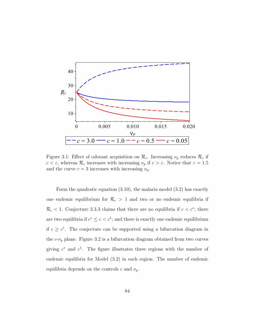
Figure 3.1: Effect of odorant acquisition on Rc. Increasing νp reduces Rc ifc < ε, whereas Rc increases with increasing νp if c > ε. Notice that ε = 1.5and the curve c = 3 increases with increasing νp.
Form the quadratic equation (3.10), the malaria model (3.2) has exactly
one endemic equilibrium for Rc > 1 and two or no endemic equilibria if
Rc < 1. Conjecture 3.3.3 claims that there are no equilibria if c < c∗; there
are two equilibria if c∗ ≤ c < c1; and there is exactly one endemic equilibrium
if c ≥ c1. The conjecture can be supported using a bifurcation diagram in
the c-νp plane. Figure 3.2 is a bifurcation diagram obtained from two curves
giving c∗ and c1. The figure illustrates three regions with the number of
endemic equilibria for Model (3.2) in each region. The number of endemic
equilibria depends on the controls c and νp.
84

Figure 3.2: Bifurcations in the c-νp plane. The solid curve is Rc = 1, whichgives c1, whereas the dashed curve is q2
1 = 4q2µmω2h(1−Rc), which gives c∗.
In addition to the disease-free equilibrium, the number of endemic equilibriais 0 or 2 for Rc < 1 and 1 for Rc > 1, depending on c and νp.
Figure 3.3: Effect of c on I∗u. We use νp = 0.2. As c increases, the number ofendemic equilibria changes according to regions 0, 2 and 1.
85
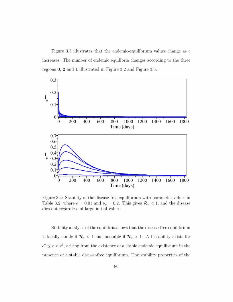
Figure 3.3 illustrates that the endemic-equilibrium values change as c
increases. The number of endemic equilibria changes according to the three
regions 0, 2 and 1 illustrated in Figure 3.2 and Figure 3.3.
Figure 3.4: Stability of the disease-free equilibrium with parameter values inTable 3.2, where c = 0.01 and νp = 0.2. This gives Rc < 1, and the diseasedies out regardless of large initial values.
Stability analysis of the equilibria shows that the disease-free equilibrium
is locally stable if Rc < 1 and unstable if Rc > 1. A bistability exists for
c∗ ≤ c < c1, arising from the existence of a stable endemic equilibrium in the
presence of a stable disease-free equilibrium. The stability properties of the
86

Figure 3.5: Stability of the endemic equilibrium with parameter values inTable 3.2, where c = 0.01 and νp = 0.002. This gives Rc > 1, and the diseasepersists regardless of small initial values.
equilibria are illustrated in the figures 3.4 and 3.5. From the figures, it can be
guessed that the disease-free equilibrium is globally stable if c < c∗, that is,
in region 0 of Figure 3.3. It remains to be shown if the endemic equilibrium is
stable for c ≥ c1, that is, in region 1 of Figure 3.3. As mentioned in Chapter
2, global stability of endemic equilibria has not been studied previously for
SEIRS models with dynamics involving mosquito bias.
87

3.5 Summary and conclusion
This study is focussed on the formulation and analysis of the mosquito-bias
model to examine the effect of a repellent for infectious humans on disease
transmission and spread. The effectiveness of a protective repellent depends
on the relative attractiveness of infectious humans who use the repellent.
The model is a modification of the artificial-feeder model of Chapter 2, with
the infectious humans progressing to the class of repellent users to prevent
bites, and without artificial feeders.
The disease control reproduction number was derived together with the
corresponding basic reproduction number to examine the effect of the controls
on disease spread. The control reproduction number is a function of the
relative attractiveness of infectious humans who use repellents and the rate
at which the repellent is obtained after the onset of the infectious stage. This
number increases linearly with the relative attractiveness of repellent users,
and changes nonlinearly with the repellent-acquisition rate.
For effective disease control based on odorant usage, the rate at which
the odorant is acquired by infected humans should be inversely proportional
to the relative attractiveness of odorant users. In other words, to reduce
disease spread, the repellent-acquisition rate should be directly proportional
to the effectiveness of the repellent. If there is increased attractiveness of
odorant users relative to non-users, then increasing the odorant-acquisition
rate for infected humans increases disease spread. Conversely, if the relative
88

attractiveness of odorant users is decreased, then increasing the odorant-
acquisition rate for infected humans decreases disease spread. There are
subcritical endemic equilibria for a relatively low attractiveness of infected
repellent users, and no endemic equilibria if the relative attractiveness of
infected repellent users is decreased beyond the subcritical value c∗, and
if the odorant-acquisition rate is maximized in the infectious stage. Thus,
disease elimination requires decreasing the relative attractiveness of infected
repellent users and increasing the repellent-acquisition rate at the same time.
89

Chapter 4
A bed-net model for Malaria
control with artificial feeders
and protective odorants
4.1 Introduction
Humans are plagued by vector-borne diseases. Every year there are more
than one billion cases and over one million deaths from vector-borne diseases
such as malaria, dengue, yellow fever, Chagas disease, Japanese encephalitis,
African trypanosomiasis, schistosomiasis, leishmaniasis and onchocerciasis,
globally [112]. The diseases are preventable through informed protective
measures, but the need for more effective disease control approaches has
come as a result of global challenges such as insecticide and drug resistance,
90
genetic variations in pathogens, and demographic changes [37].
The prevention and control of vector-borne diseases requires reducing
vector-human contacts. Many vectors are bloodsucking insects, which ingest
disease-producing pathogens during a blood meal from an infected host and
later inject it into a new host during a subsequent blood meal. Mosquitoes
are the most common disease vectors. Mosquitoes transmit malaria, dengue,
Rift Valley fever, yellow fever, Chikungunya, lymphatic filariasis, Japanese
encephalitis, and West Nile fever through bites [94, 95, 77, 109, 112]. Female
mosquitoes require a blood meal to initiate and develop eggs [23, 109].
From Chapter 1, mosquito-human contacts can be reduced by using
bed nets, protective odorants or repellents and artificial feeders. The use
of bed nets, also known as mosquito nets, has been dated to prehistoric
times. Further, the artificial-feeder model (Chapter 2) suggests that disease
control can be boosted with mosquito feeders. Simplified devices can be used
to artificially blood-feed mosquitoes. Artificial feeders can be treated with
attractants to increase their relative attractiveness to mosquitoes. Thus,
we investigate disease-control dynamics with a combination of bed nets and
artificial feeders.
Bed nets are usually treated with insecticides to divert or kill mosquitoes
and prevent mosquito-human contacts. Lengeler [56] studied the effectiveness
of insecticide-treated bed nets and concluded that bed-net usage reduced
malaria cases by 50%. Agusto et al. [2] and Buonomo [15] model bed nets
by a mosquito-human contact rate that is a linearly decreasing function of
91

bed-net usage. With bed nets, the contact rate is maximized if there are no
users, or minimized if all hosts are users. The models [2, 15] ignore bites
during the day, and so assume that bed nets are 100% effective. In reality,
bed nets are not 100% effective. They are only used by a fraction of the
population for a fraction of each day.
We develop a mathematical model of malaria control to study disease
dynamics in a region where mosquito feeders, untreated bed nets and pro-
tective odorants are used. The human population is divided into two main
classes. The first class is made up of bed-net users, and the second class is
for bed-net non-users. Protective odorants can be used by bed-net users and
this increases the relative attractiveness of bed-net non-users to mosquitoes.
Conversely, if the odorants are used by bed-net non-users, then the relative
attractiveness of bed-net users increases and mosquitoes are more biased to-
wards bed-net users. Thus, mosquito bias is modelled by a dependence of
the relative biting rates on bed-net usage. The resulting bed-net model is
analyzed to examine the effectiveness of an integrated disease-control ap-
proach where mosquito nets, protective odorants and mosquito feeders are
used. We derive a disease control reproduction number to measure transmis-
sion intensity in the presence of the proposed control methods. The model
is used to examine the effect of increasing or decreasing the relative attrac-
tiveness of bed-net users (to mosquitoes) on disease spread. It is shown that
the dynamics are completely determined by the disease control reproduction
number.
92

4.2 The bed-net model
4.2.1 Model formulation
Let N1 +N2 be the total host population where N1 is the number of bed-net
users and N2 is the number of bed-net non-users. Either protective odorants
are used by all bed-net users or the odorants are used by all bed-net non-
users. Further decompose the host population into Si, Ei, Ii, and Ri, where
Si is the number of susceptible humans; Ei is the number of latently infected
humans (noninfectious); Ii is the number of infectious humans; and Ri is the
number of recovered humans, given that i = 1 denotes bed-net users and
i = 2 denotes bed-net non-users. Thus, at time t,
N1(t) = S1(t) + E1(t) + I1(t) +R1(t),
N2(t) = S2(t) + E2(t) + I2(t) +R2(t).
People are recruited to the susceptible class through birth at a constant
rate µhλh assumed to be balanced by death, where µh is the per capita natural
death rate, and λh is the constant human population in the absence of the
disease. A proportion φ accounts for the people recruited to the susceptible
population of bed-net users, whereas 1− φ accounts for the people recruited
to the susceptible class of bed-net non-users. Susceptible individuals may
become infected through contacts with infectious mosquitoes. It is assumed
that only infectious mosquitoes can transmit infection to susceptible humans
93

through bites. Infected individuals go through a latent period, during which
they do not transmit infection. They progress from the latent stage to the
infectious stage at the rate γh. Infectious individuals recover at the rate
αh with temporary immunity to the disease. Recovered humans lose their
immunity and return to the susceptible class at the rate ρh. Although there is
evidence of disease-related deaths, the death rate is negligible compared to all
the other disease-specific parameters, and we assume this can be ignored to
simplify analysis. Thus humans leave the population only by natural death.
Let Nm be the number of female mosquitoes of which Sm are susceptible,
Em are latently infected (non-infectious) and Im are infectious. At time t,
Nm(t) = Sm(t) + Em(t) + Im(t).
Mosquitoes enter the susceptible class through birth at a constant rate
µmλm assumed to be balanced by deaths, where µm is the per capita natural
death rate, and λm is the constant mosquito population in the absence of the
disease. It is probable that the parasite enters the mosquito through biting
an infectious human. It is assumed that only infectious humans can transmit
infection to susceptible mosquitoes through bites. Infected mosquitoes go
through a latent period, during which they do not transmit infection. They
progress from the latent stage to the infectious stage at the rate γm, and
remain infectious for life. Mosquitoes leave the population only through
natural death.
94
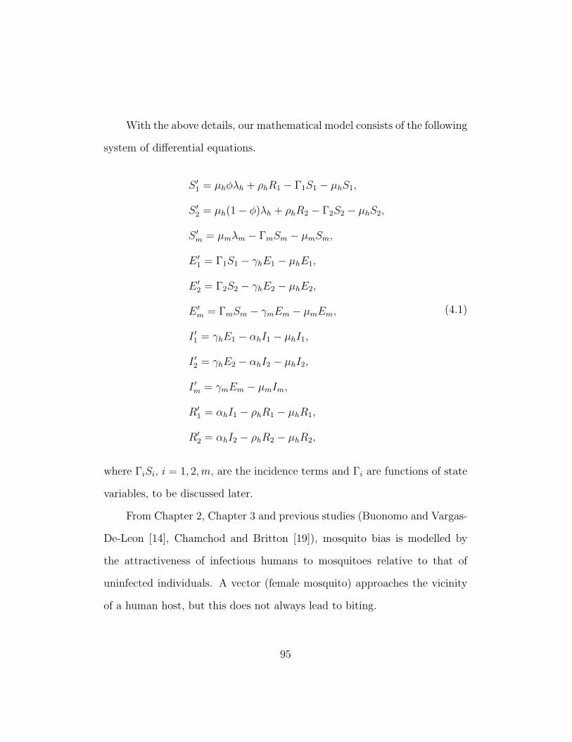
With the above details, our mathematical model consists of the following
system of differential equations.
S ′1 = µhφλh + ρhR1 − Γ1S1 − µhS1,
S ′2 = µh(1− φ)λh + ρhR2 − Γ2S2 − µhS2,
S ′m = µmλm − ΓmSm − µmSm,
E ′1 = Γ1S1 − γhE1 − µhE1,
E ′2 = Γ2S2 − γhE2 − µhE2,
E ′m = ΓmSm − γmEm − µmEm,
I ′1 = γhE1 − αhI1 − µhI1,
I ′2 = γhE2 − αhI2 − µhI2,
I ′m = γmEm − µmIm,
R′1 = αhI1 − ρhR1 − µhR1,
R′2 = αhI2 − ρhR2 − µhR2,
(4.1)
where ΓiSi, i = 1, 2,m, are the incidence terms and Γi are functions of state
variables, to be discussed later.
From Chapter 2, Chapter 3 and previous studies (Buonomo and Vargas-
De-Leon [14], Chamchod and Britton [19]), mosquito bias is modelled by
the attractiveness of infectious humans to mosquitoes relative to that of
uninfected individuals. A vector (female mosquito) approaches the vicinity
of a human host, but this does not always lead to biting.
95

Let Na be the number of artificial feeders. Let β be the average biting
rate of a female mosquito. Let ci, i = 1, 2, 3 be the probability of a mosquito
biting a bed-net user, a bed-net non-user or an artificial feeder, respectively,
given an encounter with such a host. Thus, the distribution of bites depends
on the probabilities ci ignoring the natural mosquito bias towards infectious
individuals. Given an encounter rate θ (per day), a mosquito is likely to bite
θ(c1N1 + c2N2 + c3Na)
hosts per day. Further, let b, 0 ≤ b < 1, be the fraction of each day for which
a bed net is used. Thus 1 − b is the fraction of each day without bed-net
protection, and b = 0 if the bed net is not used for the whole day.
The total daily number of potentially infectious bites from mosquitoes is
βIm. Let p1 be the probability a bite by an infected mosquito on a susceptible
human host leads to infection of the human. The incidence of new human
infections among bed-net users is Γ1S1, where
Γ1 =c1p1(1− b)βIm
c1N1 + c2N2 + c3Na
is the force of infection among bed-net users. Similarly, the incidence of new
human infections among bed-net non-users is Γ2S2, where
Γ2 =c2p1βIm
c1N1 + c2N2 + c3Na
96

is the force of infection among individuals who never use bed nets. The daily
number of bites by susceptible mosquitoes is βSm. Let p2 be the probability
a bite by a susceptible mosquito on an infected human host leads to infection
of the mosquito. The incidence of new mosquito infections is ΓmSm, where
Γm =c1p1(1− b)βI1 + c2p2βI2c1N1 + c2N2 + c3Na
is the force of infection among susceptible mosquitoes.
4.2.2 Rescaled bed-net model
We introduce the following parameters to simplify the incidence terms.
βh = p1β; βm = p2β; and c =c2c1.
Following the technique of Chapter 3, we re-write System (4.1) in a rescaled
form by scaling human and mosquito populations using λh and λm, respec-
tively. Thus, we study proportions of the populations with respect to the
constant population size in the absence of the disease. For i = 1, 2, let
Si =Siλh, Ei =
Eiλh, Ii =
Iiλh, and Ri =
Ri
λh,
for the human population; and
Sm =Smλm
, Em =Emλm
, and Im =Ihλm
,
97

for the mosquito population. Further, let
A =c3c1
Na
λhand m0 =
λmλh. (4.2)
Keeping the same notation as in System (4.1) (for simplicity), the rescaled
system consists of the following differential equations.
S ′1 = µhφ+ ρhR1 − Γ1S1 − µhS1,
S ′2 = µh(1− φ) + ρhR2 − Γ2S2 − µhS2,
S ′m = µm − ΓmSm − µmSm,
E ′1 = Γ1S1 − γhE1 − µhE1,
E ′2 = Γ2S2 − γhE2 − µhE2,
E ′m = ΓmSm − γmEm − µmEm,
I ′1 = γhE1 − αhI1 − µhI1,
I ′2 = γhE2 − αhI2 − µhI2,
I ′m = γmEm − µmIm,
R′1 = αhI1 − ρhR1 − µhR1,
R′2 = αhI2 − ρhR2 − µhR2,
(4.3)
where
Γ1 =m0(1− b)βhImN1 + cN2 + A
, Γ2 =cΓ1
1− b, Γm =
(1− b)βmI1 + cβmI2N1 + cN2 + A
. (4.4)
98
Let X = (S1, S2, Sm, E1, E2, Em, I1, I2, Im, R1, R2) denote a solution of
the system to be studied with initial data X0 = X(0). We write Si(0) = Si0,
Ei(0) = Ei0, Ii(0) = Ii0, Ri(0) = Ri0, and Ni(0) = Ni0, i = 1, 2,m.
The malaria model 4.3 is based on the following set of assumptions.
A1: There is a constant recruitment to the susceptible human population
as a result of birth, which is balanced by natural deaths.
A2: There is a constant recruitment to the susceptible mosquito population
as a result of birth, which is balanced by natural deaths.
A3: Transmission takes place only from infectious mosquitoes to susceptible
humans and from infectious humans to susceptible mosquitoes.
A4: Infected mosquitoes do not live long enough to recover from infection.
A5: Recovered humans have full immunity to the disease for a few years
after which the individuals become susceptible.
A6: Artificial feeders do not harbour or preserve disease parasites.
A7: Disease-related deaths are ignored to simplify analysis.
A8: Humans don’t switch status with regards to bed-net usage.
Assumption A6 ensures that there is no possibility for the transfer and
survival of the pathogen in the artificial feeder should an infectious mosquito
feed from the feeder, otherwise this may lead to unintended effects.
99

Assumption A7 enables analysis with constant population. There are
studies (such as [16, 20, 75, 78, 79], and Chapter 2) suggesting that the
disease-induced death may facilitate a backward bifurcation. In that case,
disease eradication may not be guaranteed even when the disease control
reproduction number is less than unity.
Table 4.1: Parameters for the bed-net model
Parameter Descriptionµh Natural death rate of humans.µm Natural death rate of female mosquitoes.βh Mosquito biting rate leading to infection of the human host.βm Mosquito biting rate leading to infection of the mosquito.γh Rate at which a human becomes infectious after infection.γm Rate at which a mosquito becomes infectious after infection.αh Rate at which a human recovers from infection.ρh Rate at which a recovered human loses partial immunity.m0 Ratio of total mosquito population to human population.b Effectiveness of bed nets (as a fraction of each day).A Ratio of adjusted number of feeders to number of humans.c Relative attractiveness of bed-net non-users to mosquitoes.φ Bed-net coverage or usage (a proportion for bed-net users).
The parameters for the model are outlined in Table 4.1. All parameters
are positive. The parameter m0 is the ratio of the total vector population
to the total host population in the absence of the disease. A is the ratio of
the adjusted number of artificial feeders to total human population when a
mosquito is equally attracted to susceptible humans and artificial feeders. c
represents the attractiveness of bed-net non-users (to mosquitoes) compared
100

to that of bed-net users. For System (4.3), c takes the following cases.
c > 1 : A mosquito is more attracted to a bed-net non-user than to a bed-net
user upon encounter, that is, the odorant is used by bed-net users.
c = 1 : A mosquito is equally attracted to a bed-net user and a bed-net
non-user upon encounter, that is, no odorant usage and mosquito bias.
c < 1 : A mosquito is less attracted to a bed-net non-user than to a bed-net
user upon encounter, that is, the odorant is used by bed-net non-users.
4.2.3 Well-posedness
By the basic theory of ordinary differential equations (Theorem 1.4.1), the
right hand side of (4.3) is differentiable on R11, which implies that a unique
solution X exists for every initial condition. Following the approaches of
Chapter 2, it can be shown that System (4.3) has positive and bounded
solutions. In fact, it is found that the positive cone R11+ is forward-invariant
and the unique solution X is positive for all t ≥ 0.
Theorem 4.2.1. For Model (4.3), the disease-free plane is invariant. All
solutions starting with Ei = Em = Ii = Im = 0 (for i=1,2) remain in the
disease-free plane for all time t > 0 with Si > 0, Sm > 0, and Ri ≥ 0.
Proof . With Ei = Em = Ii = Im = 0, i = 1, 2, it follows that Γi = Γm = 0.
Hence System (4.3) gives S ′1 = µh(φ−S1)+ρhR1, S′2 = µh(1−φ−S2)+ρhR2,
S ′m = µm(1− Sm), R′i = −(ρh + µh)Ri, and E ′i = E ′m = I ′i = I ′m = 0. Solving
101
these yields Ei = Em = Ii = Im = 0, S1 = φ− S10e−µht − R10e
−(ρh+µh)t > 0,
S2 = 1 − φ − S20e−µht − R20e
−(ρh+µh)t > 0, Sm = 1 + (Sm0 − λm)e−µmt > 0,
and Ri = Ri0e−(ρh+µh)t ≥ 0. The solutions exist in the disease-free plane and
form the disease-free set {S1, S2, Sm, R1, R2}.
Theorem 4.2.2 (Positivity of solutions). Model (4.3) is mathematically and
epidemiologically well-posed with a unique solution. Given nonnegative initial
data X0, the solution X is positive for all time t ≥ 0.
Proof . For System (4.3), suppose X0 > 0 and that at least one component
of X is negative at some time t > 0. By continuity and differentiability of X,
there must be some time t0 such that X(t) > 0 ∀t ∈ [0, t0) and one or more
components of X(t0) are zero with nonpositive derivatives. By the equation
for S ′1, if S1(t0) = 0 and µhφ+ρhR1(t0) ≤ 0, then R1(t0) < 0 and R1 must be
zero somewhere on (0, t0). Hence S1(t0) > 0. Continuing with the approach
used for the proof of Theorem 2.2.2 in Chapter 2, it is found that if X(t) > 0
on [0, t0) and any component of X(t0) is zero, then Ei, Em, Ii, Im = 0 at t0
with E ′i, E′m, I
′i, I′m = 0, i = 1, 2. From the invariance of the disease-free set
(Theorem 4.2.1) and the uniqueness of solutions, having Ei, Em, Ii, Im = 0
at t0 implies that Ei, Em, Ii, Im = 0, Si > 0, Sm > 0 and Ri ≥ 0 ∀t > 0,
contradicting the supposition that X(t) > 0 ∀t ∈ [0, t0).
Theorem 4.2.3 (Boundedness of solutions). Model (4.3) is mathematically
and epidemiologically well-posed. The unique solution X is bounded given
nonnegative initial data X0.
102

Proof . By the definitions of N1, N2 and Nm, and Equations (4.3), we obtain
N ′1 = S ′1 + E ′1 + I ′1 +R′1, N′2 = S ′2 + E ′2 + I ′2 +R′2 and N ′m = S ′m + E ′m + I ′m.
We solve the derivatives to give
N1 = φ+ (N10 − φ)e−µht,
N2 = 1− φ+ (N20 − 1− φ)e−µht,
Nm = 1 + (Nm0 − 1)e−µmt,
(4.5)
∀t ≥ 0, where N10, N20 and Nm0 are initial values. By positivity, N1, N2
and Nm are bounded between 0 and the solutions of (4.5), hence so are all
components of X (by positivity of each component).
Corollary 4.2.4 (Domain of attraction). For Model (4.3) with nonnegative
initial data X0, there exists a domain attracting all solutions X ∈ R11+ .
By theorems 4.2.2 and 4.2.3, define a domain D such that
D =
X ∈ R11
+
∣∣∣∣∣∣∣∣∣∣∣∣∣∣∣∣
S1 > 0, S2 > 0, Sm > 0, E1 ≥ 0, E2 ≥ 0, Em ≥ 0
I1 ≥ 0, I2 ≥ 0, Im ≥ 0, R1 ≥ 0, R2 ≥ 0
S1 + E1 + I1 +R1 = φ
S2 + E2 + I2 +R2 = (1− φ)
Sm + Em + Im = 1
.
It can be verified from (4.5) that for any initial data X0 ∈ D, the solution
X is always contained in the interior and boundary of D, and there are no
orbits leaving D. Thus the domain D is invariant and attracting.
103

4.3 Equilibria and their stability
4.3.1 Disease-free equilibrium
A constant solution to a system of equations is referred to as an equilibrium
solution. If in addition, Ei = Ii = 0, i = 1, 2,m, then X is referred to
as a disease-free equilibrium. Otherwise, X is referred to as an endemic
equilibrium. Below we show that System (4.3) has a unique disease-free
equilibrium, and that any endemic equilibria are strictly positive.
An equilibrium solution of Equations (4.3) satisfies
µhφ+ ρhR1 − Γ1S1 − µhS1 = 0, (4.6a)
µh(1− φ) + ρhR2 − Γ2S2 − µhS2 = 0, (4.6b)
µm − ΓmSm − µmSm = 0, (4.6c)
Γ1S1 − (γh + µh)E1 = 0, (4.6d)
Γ2S2 − (γh + µh)E2 = 0, (4.6e)
ΓmSm − (γm + µm)Em = 0, (4.6f)
γhE1 − (αh + µh)I1 = 0, (4.6g)
γhE2 − (αh + µh)I2 = 0, (4.6h)
γmEm − µmIm = 0, (4.6i)
αhI1 − (ρh + µh)R1 = 0, (4.6j)
αhI2 − (ρh + µh)R2 = 0. (4.6k)
104

Theorem 4.3.1 (Boundary Equilibria). System (4.3) has a unique disease-
free equilibrium and no other equilibria on the boundary of D.
The above theorem can be proven by following a similar approach of
Chapter 2 (see Theorem 2.3.1). For System (4.3), there exists exactly one
disease-free equilibrium. In addition, any equilibrium that exists in the
boundary of D ⊂ R11+ does so with Ei = Em = Ii = Im = Ri = 0, where
i = 1, 2, and the equilibrium is disease-free. Otherwise, the equilibrium is
strictly positive and endemic. The domain D is positively invariant and
the disease-free equilibrium in the boundary is the only equilibrium of (4.3)
without the disease. By Theorem 4.2.2 and Equations (4.6), it is straight
forward that if any of Ei, Em, Ii, Im, Ri, is positive, where i = 1, 2, then all
components of X are positive and the equilibrium is strictly positive.
Let X0 denote the disease-free equilibrium. It follows that
X0 = (φ, (1− φ), 1, 0, 0, 0, 0, 0, 0, 0, 0).
Next we investigate the stability of the disease-free equilibrium using the
Jacobian matrix of the system, evaluated at X0.
An equilibrium of Equations (4.3) is said to be (locally asymptotically)
stable if solutions with initial conditions in a sufficiently small neighbourhood
of the equilibrium asymptotically approach the equilibrium.
Epidemiologically, stability of the disease-free equilibrium implies that
small introductions of infected individuals into a population do not lead to
105

an outbreak. Thus, stability of the disease-free equilibrium can be described
using the disease control reproduction number.
Definition 4.3.1. The control reproduction number for System (4.3) is
Rc =m0βhβmγhγm[(1− b)2φ+ c2(1− φ)]
(φ+ c(1− φ) + A)2(γh + µh)(αh + µh)(γm + µm)µm. (4.7)
As seen in the previous chapters, Rc is the expected number of new
infected humans as a result of introducing one infected human in a population
at a disease-free equilibrium in the presence of disease control methods.
Theorem 4.3.2. For System (4.3), the disease-free equilibrium is locally
asymptotically stable if Rc < 1 and unstable if Rc > 1.
Proof . From Theorem 1.4.4, an equilibrium solution is locally asymptoti-
cally stable if all eigenvalues of the Jacobian matrix have negative real parts.
The Jacobian matrix evaluated at X0 has the block structure
J(X0) =
J11 J12 J13
0 J22 0
0 J32 J33
,
with submatrices
J11 =
−µh 0 0
0 −µh 0
0 0 −µm
, J13 =
ρh 0
0 ρh
0 0
,
106

J12 =
0 0 0 0 0
−m0(1− b)φβhφ+ c(1− φ) + A
0 0 0 0 0−m0c(1− φ)βhφ+ c(1− φ) + A
0 0 0−(1− b)βm
φ+ c(1− φ) + A
−cβmφ+ c(1− φ) + A
0
,
J32 =
0 0 0 αh 0 0
0 0 0 0 αh 0
, J33 =
−ρh − µh 0
0 −ρh − µh
.X0 is stable if all eigenvalues of J(X0) have negative real parts. By the
block structure of J(X0), its eigenvalues are those of J11, J22 and J33. Since,
by inspection, the eigenvalues of J11 and J33 have negative real parts, X0 is
stable if all eigenvalues of J22 have negative real parts. By the decomposition
method of van den Driessche and Watmough [106], the submatrix J22 has the
structure F − V , and all eigenvalues of J22 have negative real parts if and
only if ρ(FV −1) < 1, where ρ denotes the spectral radius. It follows that
J22 = F − V where
F =
0 0 0 0 0m0(1− b)φβh
φ+ c(1− φ) + A
0 0 0 0 0m0c(1− φ)βh
φ+ c(1− φ) + A
0 0 0(1− b)βm
φ+ c(1− φ) + A
cβmφ+ c(1− φ) + A
0
0 0 0 0 0 0
0 0 0 0 0 0
0 0 0 0 0 0
,
107

and
V =
γh + µh 0 0 0 0 0
0 γh + µh 0 0 0 0
0 0 γm + µm 0 0 0
−γh 0 0 αh + µh 0 0
0 −γh 0 0 αh + µh 0
0 0 −γm 0 0 µm
.
We compute ρ(FV −1) and set Rc = (ρ(FV −1))2. Stability follows from the
fact that ρ(FV −1) < 1 implies (ρ(FV −1))2 < 1.
In the special case where c = 1 and φ,A = 0, the control reproduction
number Rc gives the basic reproduction number, denoted R0. Thus,
R0 =m0βhβmγhγm
(γh + µh)(αh + µh)(γm + µm)µm. (4.8)
For System (4.3), R0 is the expected number of new infected humans as a
result of introducing one infected human in a population at a disease-free
equilibrium in the absence of disease control methods.
From (4.7) and (4.8), it is immediately apparent that
Rc = R0(1− b)2φ+ c2(1− φ)
(φ+ c(1− φ) + A)2. (4.9)
A, c and φ are the control parameters. Given c and φ, Rc is decreasing with
108

A, but Rc may either increase or decrease with c and φ, so they are not
necessarily good control parameters. Later we use Elasticity analysis of Rc
to examine the effectiveness of the controls.
IfRc < 1, then on average an infected human produces less than one new
human infection over the course of the infectious period in the presence of
disease control methods, and malaria will not spread. Conversely, if Rc > 1,
then each infected human produces, on average, more than one new human
infection in the presence of disease control methods and malaria can invade
the population.
4.3.2 Endemic equilibria
Theorem 4.3.3 (Existence of endemic equilibria). For the malaria model
(4.3), there are no endemic equilibria if Rc < 1 and there is exactly one
endemic equilibrium if Rc > 1.
Proof . Let X∗ = (S∗1 , S∗2 , S
∗m, E
∗1 , E
∗2 , E
∗m, I
∗1 , I
∗2 , I
∗m, R
∗1, R
∗2) be an equilib-
rium solution of System (4.3). Thus X∗ satisfies Equations (4.6). Since
N1 = S1 + E1 + I1 + R1 and N2 = S2 + E2 + I2 + R2, Equations (4.6) give
N∗1 = φ and N∗2 = 1− φ. Substituting for N1 and N2 in Equation (4.4) gives
Γ∗1 =m0(1− b)βhI∗mφ+ c(1− φ) + A
and Γ∗m =βm((1− b)I∗1 + cI∗2 )
φ+ c(1− φ) + A, (4.10)
with Γ∗2 = cΓ∗1/(1 − b). Below we solve Equations (4.6) for the endemic
equilibria. First solve for S∗1 in terms of Γ∗1, S∗2 in terms of Γ∗2, and S∗m in
109
terms of Γ∗m. It follows that
S∗1 =µhφ
ω1Γ∗1 + µh, S∗2 =
µh(1− φ)
ω1Γ∗2 + µh, and S∗m =
µmΓ∗m + µm
, (4.11)
where
ω1 =(γh + µh)(αh + µh)(ρh + µh)− γhαhρh
(γh + µh)(αh + µh)(ρh + µh).
0 < ω1 < 1 by inspection.
Express E∗1 in terms of Γ∗1 using the relationship with S∗1 from (4.6d)
and (4.11). The process continues for the rest of the state variables yielding
E∗1 =µhφΓ∗1
(γh + µh)(ω1Γ∗1 + µh), I∗1 =
ω2φΓ∗1(ω1Γ∗1 + µh)
,
E∗2 =µh(1− φ)Γ∗2
(γh + µh)(ω1Γ∗2 + µh), I∗2 =
ω2(1− φ)Γ∗2(ω1Γ∗2 + µh)
,
E∗m =µmΓ∗m
(γm + µm)(Γ∗m + µm), I∗m =
γmΓ∗m(γm + µm)(Γ∗m + µm)
,
R∗1 =ω2αhφΓ∗1
(ρh + µh)(ω1Γ∗1 + µh), R∗2 =
ω2αh(1− φ)Γ∗2(ρh + µh)(ω1Γ∗2 + µh)
,
(4.12)
where
ω2 =γhµh
(γh + µh)(αh + µh). (4.13)
In the next step, I∗1 , I∗2 , I∗m, Γ∗1, Γ∗2, and Γ∗m are used to obtain an equation
involving only Γ∗1. Substitute I∗1 and I∗2 (4.12) into Γ∗m (4.4), and use the
relation Γ∗2 = cΓ∗1/(1− b), to yield
Γ∗m =βmΓ∗1ω2
(φ+ c(1− φ) + A)
((1− b)φω1Γ∗1 + µh
+c2(1− φ)
ω1cΓ∗1 + (1− b)µh
). (4.14)
110

Using Γ∗m, I∗m and Γ∗1 gives a cubic equation q2Γ∗31 + q1Γ
∗21 + q0Γ
∗1 = 0 with
the coefficients
q2 =ω1ω2cβm((1− b)φ+ c(1− φ))
(φ+ c(1− φ) + A)+ cµmω
21,
q1 =µhω2cβm((1− b)2φ+ c2(1− φ))
(φ+ c(1− φ) + A)+ µmµhω1(1− b+ c)(1− ψ0Rc),
q0 = µmµ2h(1− b)(1−Rc),
where
ψ0 =c(1− b)2φ+ c2(1− b)(1− φ)
(1− b+ c)((1− b)2φ+ c2(1− φ)).
By inspection, 0 < ψ0 < 1 and q2 is always positive.
The cubic equation has a trivial solution, Γ∗1 = 0, which corresponds to the
disease-free equilibrium. The non-trivial solutions satisfy
q2Γ∗21 + q1Γ
∗1 + q0 = 0. (4.15)
If Rc < 1, then q1 > 0 and q0 > 0, and since q2 > 0, Descartes’ Rule of Signs
(Theorem 1.4.3) suggests that equation (4.15) has no positive real roots.
Conversely, if Rc > 1, then q0 < 0 and, by Theorem 1.4.3, the equation has
exactly one positive real root regardless of the sign of q1.
Let Γ∗1a and Γ∗1b denote the roots of equation (4.15) given by
Γ∗1a =−q1 +
√q21 − 4q2q0
2q2and Γ∗1b =
−q1 −√q21 − 4q2q0
2q2.
111

Equation (4.15) has no positive real roots if Rc < 1 and there is exactly one
positive real root if Rc > 1. In fact Γ∗1a > 0 and Γ∗1b < 0 if Rc > 1. Compute
Γ∗1, Γ∗2 and Γ∗m for substitution into Equations (4.11) and (4.12). It follows
that there is exactly one endemic equilibrium solution if Rc > 1, and the
equilibrium coexists with an unstable disease-free equilibrium.
Conjecture 4.3.4 (Global stability of the disease-free equilibrium). For
System (4.3), the disease-free equilibrium is globally asymptotically stable if
Rc < 1 and unstable if Rc > 1.
As discussed in Chapter 2, global-stability analysis of endemic equilibria
for SEIRS models with vector bias requires further consideration. For the
SIS vector-bias model of Buonomo and Vargas-De-Leon [14], it is shown that
the endemic equilibrium is globally stable if R0 > 1. Some SEIR, SEI, SI or
SIR models without mosquito bias ([54], [113], [114]) have a globally stable
endemic equilibrium if R0 > 1. System (4.3) has no endemic equilibria for
Rc < 1, hence we conjecture that the disease-free equilibrium is globally
stable in the absence of endemic equilibria (Conjecture 4.3.4). Later we use
numerical simulations to illustrate the stability properties of the equilibria.
4.3.3 Elasticity analysis of Rc
Elasticity of a function is the ratio of the percentage change in the function’s
output with respect to the percentage change in its input, for infinitesimal
changes from a point (Hanoch [39], Sydsaeter and Hammond [99]). In this
112

section, Elasticity analysis measures the ratio of the relative change in Rc to
the relative change in each of the control parameters A, c and φ.
Definition 4.3.2 (Sydsaeter and Hammond [99]). Suppose a function Rc is
differentiable at x. If Rc(x) 6= 0, the elasticity of Rc with respect to x is
ElxRc(x) =x
Rc(x)R′c(x).
From Equation (4.9), it is seen that Rc is continuous in its parameters.
Below are the Elasticities of Rc with respect to the controls A, c and φ.
ElARc =A
Rc
∂Rc
∂A=
−2A
φ+ c(1− φ) + A,
ElcRc =c
Rc
∂Rc
∂c=
2c(1− φ)(c(A+ φ)− (1− b)2φ)
(φ+ c(1− φ) + A)((1− b)2φ+ c2(1− φ)),
ElφRc =φ
Rc
∂Rc
∂φ=φ(((1− b)2 − c2)(c+ A− (1− c)φ)− 2(1− c)c2)
((1− b)2φ+ c2(1− φ))(φ+ c(1− φ) + A).
Since Rc is positive for positive parameters, the elasticities ElARc, ElcRc
and ElφRc define the percentage change as well as the slope of Rc with
respect to A, c and φ, respectively, when other parameters are fixed.
ElARc = 0 for A = 0, and ElARc < 0 for all A > 0, which implies that
Rc decreases with A. The elasticity with respect to A is monotone in A,
ranging from 0 to −2 as A increases. For large A (relative to c), a percentage
change in A leads to a 2% change in Rc.
113

ElcRc = 0 for c = 0 or φ = 1 or c = cmax, where
cmax =(1− b)2φ
(A+ φ)< 1.
Since the denominator of ElcRc is positive, ElcRc < 0 for c < cmax and
ElcRc > 0 for c > cmax. This implies that Rc (versus c) has a local minimum
at c = cmax. Thus cmax is an optimal target for c. c should be increased if it
is below cmax and decreased if it is above cmax.
ElφRc = 0 if φ = 0 or φ = φmin where
φmin =c+ A
1− c− 2c2
(1− b)2 − c2.
Rc (versus φ) has a local maximum at φmin if (1− c)((1− b)2 − c2) > 0 and
a local minimum at φmin if (1 − c)((1 − b)2 − c2) < 0. The latter holds if
and only if 1 − b < c < 1, which gives φmin > 1 and hence φmin does not
exist for φ ∈ [0, 1]. As a result, the optimal value for φ is 1 if 1− b < c < 1
and φ should be increased to 1. Conversely, the optimal value is 0 or 1 if
(1− c)(1− b− c) > 0 and φ should be decreased to 0 or increased to 1.
4.4 Discussion of results
Given below are the results of the bed-net model together with supporting
figures. The figures are obtained using parameter values in Table 4.2. A
discussion of the values and range can be found in Section 2.4.
114

Table 4.2: Parameter values used for simulations
Parameter Value Range Sourceµh 0.00004 per day (0, 0.001) §2.4µm 0.065 per day (0.001, 0.1) [20]βh 0.02 per day (0.001, 0.2) [20]βm 0.192 per day (0.005, 0.4) [20]γh 0.10 per day (0.06, 0.2) [68]γm 0.09 per day (0.02, 0.4) [20]αh 0.0035 per day (0.001, 0.02) [68]ρh 0.0005 per day (0, 0.01) [20]m0 2 mosquitoes per person (0, 10) §2.4b 0.5 (0, 1)A 0−∞ (0,∞) §2.4c 0−∞ (0,∞) §2.4φ 0− 1 (0, 1)
The control reproduction number determines the dynamics of the disease
in response to the control parameters A, c and φ. From Theorem 4.3.3,
System (4.3) has no endemic equilibria if Rc < 1, and the system has exactly
one endemic equilibrium in addition to the disease-free equilibrium if Rc > 1.
Setting Rc = 1 gives a threshold condition for the existence of the equilibria.
Figure 4.1 illustrates the curve Rc = 1 in the φ-A plane for c = 2.0, c = 1.0,
and c = 0.2. Points in the region above the curve give Rc < 1, which
is when the system has only the disease-free equilibrium, and the disease
cannot spread or invade the population.
From Equation 4.9, we write Rc = Rc(A, c, φ). Note that Rc(A, c, 1) is
independent of c. This implies that at φ = 1, Rc is purely determined by A
115

Figure 4.1: Bifurcation in the φ-A plane. Each level curve gives Rc = 1 for agiven c. For each curve, points in the region above the curve satisfy Rc < 1,and points below each curve satisfy Rc > 1.
for all c. Rc > 1 for the region below the curve in Figure 4.1 and the disease
can spread or invade the population. The endemic region (below the curve)
can be reduced by decreasing c. Reducing c decreases the height of the curve
at φ = 0, hence Rc < 1 can be obtained easily if A is large relative to c.
Thus Figure 4.1 illustrates that eradication is easily done at a relatively low
attractiveness of bed-net non-users.
Local-stability analysis suggest that the disease-free equilibrium is stable
if Rc < 1 and unstable if Rc > 1 (Theorem 4.3.2). Theorem 4.3.3 guarantees
that System (4.3) has an unstable disease-free equilibrium and exactly one
116

endemic equilibrium for Rc > 1. The stability properties of the equilibria are
illustrated in Figures 4.2, 4.3 and 4.4. In Figure 4.2, all solutions appear to
converge to the disease-free set for Rc < 1 regardless of large initial values.
In Figure 4.3 and Figure 4.4, the solutions appear to converge to the endemic
equilibrium for Rc > 1 regardless of small initial values.
Figure 4.2: Stability of the disease-free equilibrium. Rc < 1 with A = 2,c = 0.5 and φ = 0.5. The solutions converge to the disease-free equilibriumregardless of large initial values.
By Elasticity ElARc, Rc decreases with A. This means that increasing
A can slow disease spread. Eradication is easily done if A is large relative
to c. Recall from Equation (4.2) that A is the number of feeders scaled by
the human population and the relative attraction of mosquitoes to feeders.
Hence, increasing A means increasing the number or the attractiveness of the
feeders relative to humans. Thus, disease spread can be stopped by increasing
the number or attractiveness of artificial feeders relative to humans.
117

Figure 4.3: Malaria prevalence for bed-net users (I1). Rc > 1 with A = 2,c = 2 and φ = 0.5. The endemic equilibrium appears to be stable regardlessof small initial values.
Figure 4.4: Malaria prevalence for bed-net non-users (I2). Rc > 1 withA = 2, c = 2 and φ = 0.5. The endemic equilibrium appears to be stableregardless of small initial values.
118
By Elasticity ElcRc, Rc decreases with c for c < cmax and increases with
c for c > cmax. To slow or stop disease spread, the relative attractiveness of
bed-net non-users should be increased if it is below cmax and decreased if it
is above cmax. By inspection cmax < 1. Thus, the optimal value of c exists
only for a relatively low attractiveness of bed-net non-users.
From ElφRc, Rc increases and decreases with φ for 0 < φ < φmin and
φmin < φ < 1, respectively. The value of φmin depends on A and c. By
inspection, if A is small or negligible and c is large, then Rc is large but
φmin is small or negative. If A is small or negligible and c is small, then Rc is
large and φmin is large. φmin large means that it is difficult to reduce Rc with
bed nets alone, whereas φmin small implies that it is easy to reduce Rc with
bed nets alone. It follows that if mosquitoes are more attracted to bed-net
non-users than to bed-net users (if the repellent is used by bed-net users),
then increasing bed-net coverage decreases Rc, but Rc is always large.
With bed nets alone, disease eradication is difficult. From Equation 4.9,
if A = 0 and c = 1, thenRc(0, 1, φ) = R0[(1−b)2φ+(1−φ)]. For the case with
no bed-net usage, Rc(0, 1, 0) = R0. For the case with full bed-net coverage,
Rc(0, 1, 1) = R0(1−b)2. The disease cannot be eradicated with bed nets alone
if R0(1− b)2 > 1, that is, if R0 > 4, assuming b = 0.5. Estimates for R0 are
16.63 and 24.94 from Chapter 2 and Chapter 3, respectively. For the bed-net
model (4.6), R0 = 19.44, and eradication is possible if 19.44(1 − b)2 < 1.
This holds if φ = 1 and b > 0.94, that is, if all people use bed nets for more
than 94% of the day, which may not be realistic.
119

Figure 4.5 illustrates the effect of φ on Rc for the given values of c with
A = 0. It is seen that Rc is largely decreasing with φ as c decreases. Notice
that A is negligible and Rc is large for all φ. At φ = 1, Rc attains a value
determined purely by A for all c. In Figure 4.6, the effect of φ on Rc is
illustrated with A = 0.1. It is seen that Rc is largely decreasing with φ as c
decreases. Notice that A is small (A = 0.1) and Rc is still large for all φ.
Figure 4.5: Effect of φ on Rc with A negligible. Let A = 0. At φ = 1, Rc
attains a value determined by A for all c.
If A is large and c is large, then Rc is large but φmin is small or negative.
If A is large and c is small, then Rc is small and φmin is large. It follows
that if mosquitoes are less attracted to bed-net non-users than to bed-net
users (if the repellent is used by bed-net non-users), then increasing bed-net
120
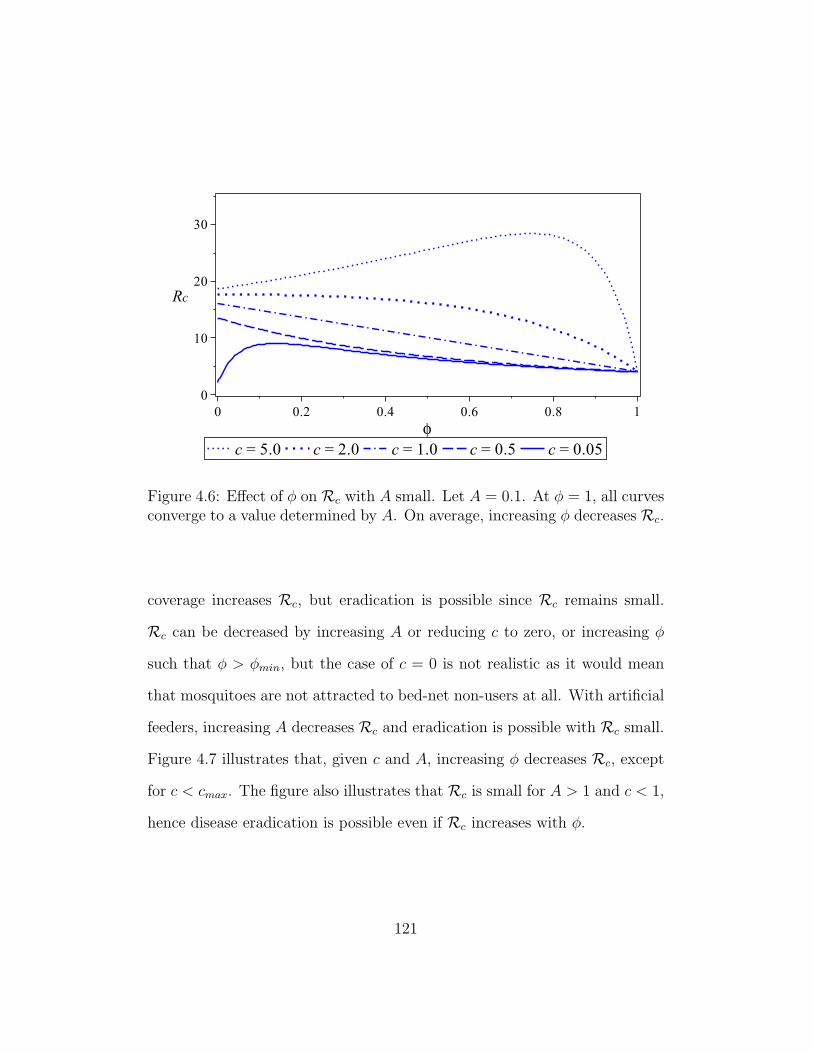
Figure 4.6: Effect of φ on Rc with A small. Let A = 0.1. At φ = 1, all curvesconverge to a value determined by A. On average, increasing φ decreases Rc.
coverage increases Rc, but eradication is possible since Rc remains small.
Rc can be decreased by increasing A or reducing c to zero, or increasing φ
such that φ > φmin, but the case of c = 0 is not realistic as it would mean
that mosquitoes are not attracted to bed-net non-users at all. With artificial
feeders, increasing A decreases Rc and eradication is possible with Rc small.
Figure 4.7 illustrates that, given c and A, increasing φ decreases Rc, except
for c < cmax. The figure also illustrates that Rc is small for A > 1 and c < 1,
hence disease eradication is possible even if Rc increases with φ.
121

Figure 4.7: Effect of φ on Rc with A large. Let A = 2. The values of Rc
have reduced compared to the values with A small or negligible. Increasingφ decreases Rc, except for the curve with c < cmax.
4.5 Conclusion
The bed-net model allows a critical analysis of a multifaceted disease-control
approach to examine the effect of bed nets, protective odorants and mosquito
feeders on disease spread using the control reproduction number. Protective
odorants are used by all bed-net users or all bed-net non-users. Elasticity
analysis of Rc is used to examine how changes in the control parameters A,
c and φ effect disease spread.
Our analysis shows that increasing artificial feeders decreases disease
spread. Previously, Buonomo [15] suggested that increasing relative mosquito
122

attraction towards infected humans may negatively impact the response of
malaria dynamics to bed-net usage. We have shown that such negative effects
associated with increasing bed-net usage can be offset by increasing artificial
feeders and encouraging bed-net non-users to use protective odorants.
For a relatively high mosquito attraction to non-users, increasing bed
nets can worsen disease spread, except if a threshold proportion is reached.
Agusto et al. [2] suggested that if 75% of the population were to use bed
nets, malaria could be eliminated, but result ignores the exposure of bed-net
users to mosquitoes. We have shown that 100% bed-net coverage does not
guarantee disease eradication. The disease persists with bed nets alone. For
a relatively low attractiveness of bed-net non-users, the negative effects of
increasing bed-net coverage are limited by a reduced spread. To achieve this,
bed-net non-users can use protective odorants. We conclude that disease
spread can be stopped using a multifaceted approach where bed nets and
artificial feeders are used, and the relative mosquito attraction towards bed-
net non-users is reduced by encouraging the use of protective odorants.
123

Chapter 5
Results and Future work
5.1 Summary
Vector behaviour influences the speed of disease spread among humans. The
biting behaviour of mosquitoes, expressed by nonrandom feeding, involves
bias towards hosts with special characteristics as discussed in Chapter 1.
Recent studies show that mosquitoes are more attracted to infected humans
than to uninfected individuals [27, 45, 52, 93]. This suggests that mosquito
bias can influence disease spread among populations. In order to eradicate
vector-borne diseases, it is important to influence vector-host interactions.
For mosquito-borne pathogens such as malaria, dengue, Rift Valley fever,
yellow fever, Chikungunya, lymphatic filariasis, Japanese encephalitis, and
West Nile fever, it is important to influence mosquito bias.
As discussed in Chapter 1, targeting mosquito bias requires a tactical
124

disease control approach with artificial feeders for mosquitoes, protective
odorants and bed nets. A mosquito’s detector of a host can be targeted
using attractants (Potter [83] and Tauxe et al. [101]) or protective odorants.
By this approach, attractants can be applied to artificial feeders such as
glytubes (Costa-da-Silva et al. [25]) to increase mosquito attraction to the
feeders. Further, several studies [2, 15, 22, 40, 111, 112] have suggested that
people can acquire protection against mosquito bites through regular use of
bed nets. To study the effectiveness of such a multifaceted control approach,
three mathematical models are developed where people are the hosts and
mosquitoes are the vectors.
For the artificial-feeder model (Chapter 2), mosquito bias is modelled
by the relative attractiveness of infectious humans to mosquitoes, keeping
in mind that this can be manipulated by disease [27, 45, 52, 93] or man
[1, 69, 83, 101]. The model is used to study the effect of influencing mosquito
bias on malaria transmission and spread in the presence of artificial feeders.
Our analysis suggests that decreasing the attractiveness of infectious humans
relative to uninfected individuals, facilitates disease eradication. Artificial
feeders reduce disease spread. Malaria can be eradicated through the use of
artificial feeders alone, but eradication is easily done if mosquitoes are more
attracted to uninfected hosts than to infectious individuals.
Our second model is a modification of the artificial-feeder model without
the artificial feeders, where there is an additional class of infectious humans
who have not acquired a protective odorant to prevent bites. The resulting
125

mosquito-bias model is analyzed to examine how the odorant-acquisition rate
for infectious hosts, affects disease spread. The effectiveness of the repellent
depends on the relative attractiveness of the user. Our analysis suggests that,
in order to stop disease spread using the odorant, the odorant-acquisition
rate should be inversely proportional to the relative attractiveness of the
odorant-user. Thus, disease spread can be stopped by minimizing the rela-
tive attractiveness of infectious humans while maximizing the rate at which
infectious individuals acquire the protective repellent.
The bed-net model (Chapter 4) combines the use of artificial feeders
with the use of untreated bed nets, where a proportion of the human popula-
tion accounts for bed-net users. The model assumes the case where bed-net
users or bed-net non-users can acquire protective odorants. Mosquito bias
is modelled by a dependence of the relative biting rates on bed-net usage.
The resulting bed-net model is used to study the effect of untreated bed
nets, protective odorants and artificial feeders on disease transmission and
spread. Our analysis suggests that increasing bed-net coverage increases dis-
ease transmission and spread if mosquitoes are more attracted to bed-net
non-users than to bed-net users. The disease can be eliminated by increasing
bed-net coverage and attractive mosquito feeders while reducing the relative
attractiveness of bed-net non-users using protective odorants.
126

5.2 Results and Implications
We note from Chapter 1 that ‘infectious’ hosts and vectors are carriers
of transmissible gametocyte stages of malaria parasites, whereas uninfected
individuals and carriers of non-transmissible stages are referred to as being
‘noninfectious’. We also note that the disease control reproduction number
is a measure of transmission intensity in the presence of the controls. The
results and epidemiological implications of the models studied in the previous
sections include (and are not limited to) the following.
RE1: From Chapter 2, increasing A relative to λh switches the direction of
bifurcation from backward to forward and decreases the disease control
reproduction number Rc. Malaria can be effectively controlled with
artificial feeders by increasing the number and attractiveness of the
feeders relative to humans.
RE2: From Chapters 2 and 3, decreasing c decreases Rc and vanishes all
endemic equilibria. Malaria can be effectively controlled by decreasing
the relative attractiveness of infectious individuals.
RE3: Chapters 2 and 3 show that mosquito bias complicates disease control.
Decreasing c below c1 gives two endemic equilibria, but no endemic
equilibria exist for c < c∗, where c∗ ≤ c1. Thus, disease spread can be
stopped by minimizing the relative attractiveness of infectious humans
and maximizing the odorant-acquisition rate at the same time.
127

RE4: Bed nets are beneficial in controlling mosquito-borne pathogens, but
the method does better in the presence of artificial feeders. With bed
nets alone, disease eradication is less likely because humans use bed
nets for only a fraction of each day. Even with 100% bed-net coverage,
the bed-net model in Chapter 4 suggests that disease eradication is not
guaranteed for diseases with R0 > 4, unless bed nets are combined
with other disease-control methods.
RE5: Bed-net users who also use protective repellents increase disease spread.
For a relatively high mosquito attraction to non-users, increasing bed
nets can worsen disease spread, except if a threshold proportion is
reached. The disease persists with bed nets alone. The negative effects
associated with increasing bed-net usage can be off-set by increasing
mosquito feeders and reducing the attractiveness of bed-net non-users
to facilitate disease eradication.
RE6: Following the above results, disease-control outcomes are influenced by
the attractiveness of hosts to mosquitoes. Increasing the attractiveness
of infected and unprotected humans increases the reproduction number
and hence the speed of disease spread. Decreasing the attractiveness to
zero can stop disease spread, but this may not be realistic. A tactical
disease-control approach should aim at decreasing the attractiveness of
infectious humans to mosquitoes by encouraging the use of protective
odorants, artificial feeders, and optimizing bed-net coverage.
128

Our mathematical models are applicable to all mosquito-borne diseases. The
proposed disease controls can be applied to all vector-borne pathogens. The
multifaceted disease-control approach based on the proposed controls can be
used to facilitate eradication. We conclude that the transmission and spread
of mosquito-borne pathogens can be stopped by using artificial feeders that
are attractive to mosquitoes, by increasing repellent-usage throughout the
infectious stage, and by ensuring optimal bed-net coverage with protective
odorants for all bed-net non-users.
5.3 Future work
The analysis of the three mathematical models can be improved in future to
better understand disease dynamics in the presence of the proposed controls.
The models follow the SEIRS framework with a large parameter space, which
complicates some analyses.
SEIRS vector bias models have not been studied previously and there are
no analytic global-stability results for the endemic equilibria. The results are
available for SIS vector-bias models (Buonomo and Vargas-De-Leon [14]), and
other models without mosquito bias [54, 55, 113, 114]. The authors use the
geometric method for global-stability analysis due to Li and Muldowney [57]
or the method of Lyapunov functions to show that the endemic equilibrium
is globally stable in the domain of attraction if R0 > 1. For the SEIRS
models developed in this study, global-stability analysis is cumbersome due
129

to the nonlinearities and a large control-parameter space. With supporting
illustrations, the endemic equilibrium is conjectured to be globally stable for
Rc > 1. The analysis is left as part of future work.
The results of the artificial-feeder model and the mosquito-bias model
suggest that increasing mosquito attraction towards infected humans in-
creases disease spread. Previously, Kingsolver [48] suggested that models
with random choice or consistent preference predict either a stable disease-
free equilibrium or a stable endemic equilibrium, but increasing the consistent
host preference makes it easier to obtain a stable endemic equilibrium rel-
ative to random choice models. Chapter 4 ignores mosquito bias towards
infectious hosts. Increasing mosquito attraction of bed-net users facilitates
disease eradication. It is not clear how the relative attractiveness of infectious
hosts affects the stability of the equilibria.
In Chapter 4, the bed-net model assumes that there is no disease-induced
death. This was a special case to simplify analysis of disease control options
with a large model. From the models of Chapter 2 and 3, the disease-induced
death facilitates the existence of subcritical endemic equilibria. The bed-net
model can be revisited in future to find out the effect of the disease-induced
death rate on the results of the model.
All in all, the models present challenging opportunities in mathematical
modelling and disease control which can be explored in future to improve the
effectiveness of disease control methods.
130

Bibliography
[1] N.L. Achee, M.J. Bangs, R. Farlow, G.F. Killeen, S. Lindsay, J.G. Logan,
S.J. Moore, M. Rowland, K. Sweeney, S.J. Torr, L.J. Zwiebel and J.P.
Grieco, Spatial repellents: from discovery and development to evidence-
based validation, Malaria Journal 2012, 11:164.
[2] F.B. Agusto, S.Y. Del Valle, K.W. Blayneh, C.N. Ngonghala, M.J.
Goncalves, N. Li, R. Zhao, and H. Gong, The impact of bed-net use
on malaria prevalence, NIH-PA J Theor. Biol., 320 (2013), 58-65.
[3] R.M. Anderson and R.M. May, Mathematical epidemiology, Oxford Uni-
versity Press, Oxford, 1991.
[4] R.M. Anderson and R.M. May, Infectious diseases of humans: dynamics
and control, Oxford University Press, London, 1991.
[5] S.J. Aneke, Mathematical modelling of drug resistant malaria parasites
and vector populations, Math. Meth. Appl. Sci., 25 (2002), 335-346.
131

[6] J. Arino, C. Bowman, A. Gumel, and S. Portet, Effect of pathogen-
resistant vectors on the transmission dynamics of a vector-borne disease,
Journal of Biological Dynamics, 1 (2007), 320-346.
[7] J.L. Aron and R.M. May, The population dynamics of malaria, in: The
Population Dynamics of Infectious Diseases. Theory and Applications,
R.M. Anderson (Ed.), Chapman and Hall, London, 1982, 139-179.
[8] J.L. Aron, Dynamics of Acquired Immunity Boosted by Exposure to In-
fection, Math. Biosc., 64 (1983), 249-259.
[9] J.L. Aron, Acquired immunity dependent upon exposure in an SIRS epi-
demic model, Math. Biosc., 88 (1988), 37-47.
[10] J.L. Aron, Mathematical modelling of immunity to malaria, Math.
Biosc., 90 (1988), 385-396.
[11] N.A.V. Beare, T.E. Taylor, S.P. Harding, S. Lewallen, and M.E.
Molyneux, Malarial Retinopathy: A Newly Established Diagnostic Sign
In Severe Malaria, Am. J. Trop. Med. Hyg., 75 (2006), 790-797.
[12] F. Brauer and P. van den Driessche, Models of transmission of diseases
with immigration of infectives, Math. Biosci., 171 (2001), 143-154.
[13] F. Brauer, Mathematical epidemiology is not an oxymoron, BMC Public
Health, 9 (2009), (Suppl 1):S2.
132

[14] B. Buonomo and C. Vargas-De-Leon, Stability and bifurcation analysis of
a vector-bias model of malaria transmission, Mathematical Biosciences,
242 (2013), 59-67.
[15] B. Buonomo, Analysis of a malaria model with mosquito host choice
and bed-net control, University of Naples Federico II, Naples, 2013,
arXiv:1311.3209 [math.CA].
[16] L-M. Cai, A.A. Lashari, I.H. Jung, K.O. Okosun, and Y.I. Seo, Mathe-
matical Analysis of a Malaria Model with Partial Immunity to Reinfec-
tion, Abstract and Applied Analysis, 2013, Article ID 405258, 17 pages,
doi:10.1155/2013/405258.
[17] A.F. Carey and J.R. Carlson, Insect olfaction from model systems to
disease control, Proc. Natl. Acad. Sci., USA, 108 (2011), 12987-12995.
[18] C. Castillo-Chavez and B. Song, Dynamical Models of Tuberculosis and
their Applications, Math. Biosc. and Eng., 1 (2004), 361-404.
[19] F. Chamchod, N.F. Britton, Analysis of a vector-bias model on malaria
transmission, Bull. Math. Biol., 73 (2011), 639-657.
[20] N. Chitnis, Using mathematical models in controlling the spread of
malaria, Ph.D. Thesis, University of Arizona, Tucson, Arizona, 2005.
[21] N. Chitnis, J.M. Cushing, and J.M. Hyman, Bifurcation analysis of a
mathematical model for malaria transmission, SIAM Journal of Appl.
Math., 67 (2006), 24-45.
133

[22] N. Chitnis, A. Schapira, T. Smith, and R. Steketee, Comparing the
Effectiveness of Malaria Vector-Control Interventions Through a Math-
ematical Model, Am. J. Trop. Med. Hyg., 83 (2010), 230-240.
[23] A.N. Clements, The biology of mosquitoes, Chapman and Hall, London,
1992, 509 pp.
[24] A. Clemons, M. Haugen, E. Flannery, M. Tomchaney, K. Kast, C. Ja-
cowski, C. Le, A. Mori, W.S. Holland, J. Sarro, D. Severson, and M.
Duman-Scheel, Aedes aegypti: an Emerging Model for Vector Mosquito
Development, Cold Spring Harbor Protocols, 2010, pdb.emo141.
[25] A.L. Costa-da-Silva, F.R. Navarrete, F.S. Salvador, M. Karina-Costa,
R.S. Ioshino, D.S. Azevedo, D.R. Rocha, C.M. Romano, and M.L. Ca-
purro, Glytube: A Conical Tube and Parafilm M-Based Method as a
Simplified Device to Artificially Blood-Feed the Dengue Vector Mosquito,
Aedes aegypti, PLoS One, 8(1) (2013), e53816.
[26] A.L. Costa-da-Silva, D.O. Carvalho, B.B. Kojin, and M.L. Capurro,
Implementation of the Artificial Feeders in Hematophagous Arthropod
Research Cooperates to the Vertebrate Animal Use Replacement, Reduc-
tion and Refinement (3Rs) Principle, J Clin Res Bioeth, 2014, 5:1.
[27] C.M. De Moraes, N.M. Stanczyk, H.S. Betz, H. Pulido, D.G. Sim, A.F.
Read, M.C. Mescher, Malaria-induced changes in host odors enhance
mosquito attraction, PNAS, 2014, DOI:10.1073/pnas.1405617111.
134

[28] A.P.K. De Zoysa, C. Mendis, A.C. Gamage-Mendis, S. Weerasinghe,
P.R.J.Herath, and K.N. Mendis, A mathematical model for Plasmodium
vivax malaria transmission: estimation of the impact of transmission-
blocking immunity in an endemic area, Bulletin of the World Health
Organization, 69 (1991), 725-734.
[29] O. Diekmann and J.A.P. Heesterbeek, Mathematical epidemiology of
infectious diseases: model building, analysis and interpretation, Wiley,
New York, 2000.
[30] K. Dietz, L. Molineaux, and A. Thomas, A malaria model tested in the
African savannah, Bull. World Health Organ., 50 (1974), 347-357.
[31] K. Dietz, Epidemics: the fitting of the first dynamic models to data,
Journal of Contemporary Mathematical analysis, 44 (2009), 97-104.
[32] L. Edelstein-Keshet, Mathematical Models in Biology, SIAM, Random
House, New York, 2005.
[33] J. Edman, J. Day, and E. Walker, Vector-host interplay - factors affect-
ing disease transmission, in: Ecology of mosquitoes, L.P. Lounibos, J.R.
Rey, and J.H. Frank, (Eds.), Chapman and Hall, NY, 1985, 273-285.
[34] M. Egeth and R. Kurzban, Artificial natural selection: can supplemen-
tal feeding domesticate mosquitoes and control mosquito-borne diseases?,
Evol. Psychol., 10 (2012), 602-610.
135

[35] L. Esteva, A.B. Gumel, and C. Vargas-De-Leon, Qualitative study of
transmission dynamics of drug-resistant malaria, Mathematical and
Computer Modelling, 50 (2009), 611-630.
[36] S.M. Garba, A.B. Gumel, M.R.A. Bakar, Backward bifurcations in
dengue transmission dynamics, Math. Biosc., 215 (2008), 11-25.
[37] D.J. Gubler, Resurgent Vector-Borne Diseases as a Global Health Prob-
lem, Emerging Infectious Diseases, 4 (1998), 442-450.
[38] J.L. Gallup and J.D. Sachs, The Economic Burden Of Malaria, Am. J.
Trop. Med. Hyg., 64 (2001), 85-96.
[39] G. Hanoch, The elasticity of scale and the shape of average costs, Amer-
ican Economic Review, 65 (1975), 492-497.
[40] W.A. Hawley, F.O. ter Kuile, R.S. Steketee, B.L. Nahlen, D.J. Terlouw,
J.E. Gimnig, Y.P. Shi, J.M. Vulule, J.A. Alaii, A.W. Hightower, M.S.
Kolczak, S.K. Kariuki, and P.A. Phillips-Howard, Implications of the
western Kenya permethrin-treated bed net study for policy, program im-
plementation, and future research, Amer. Journal of Trop. Med. and
Hygiene, 68 (2003), 168-173.
[41] J.A.P. Heesterbeek and K. Dietz, The concept of R0 in epidemic theory,
Statistica Neerlandica, 50 (1996), 89-110.
[42] J.A.P. Heesterbeek, A brief history of R0 and a recipe for its calculation,
Acta Biotheoretica, 50 (2002), 189-204.
136

[43] H.W. Hethcote, The mathematics of infectious diseases, SIAM Review,
42 (2000), 599-653.
[44] G.R. Hosack, P.A. Rossignol, and P. van den Driessche, The control of
vector-borne disease epidemics, J Theor. Biol., 255 (2008), 16-25.
[45] M. Kelly, C-Y. Su, C. Schaber, J.R. Crowley, F-F. Hsu, J.R. Carl-
son, A.R. Odom, Malaria parasites produce volatile mosquito attractants,
mBio, 6 (2015), e00235-15, DOI:10.1128/ mBio.00235-15.
[46] W.O. Kermack and A.G. McKendrick, A contribution to the mathemat-
ical theory of epidemics, Proceedings of the Royal Society of London
Series A, 115 (1927), 700-721.
[47] G.F. Killeen and T.A. Smith, Exploring the contributions of bed nets,
cattle, insecticides and excitorepellency to malaria control: a determin-
istic model of mosquito host-seeking behaviour and mortality, Trans R
Soc Trop Med Hyg., 101 (2007), 867-880.
[48] J.G. Kingsolver, Mosquito Host Choice and the Epidemiology of Malaria,
American Naturalist, 130 (1987), 811-827.
[49] J.C. Koella, On the use of mathematical models of malaria transmission,
Acta Tropica, 49 (1991), 1-25.
[50] J.C. Koella and R. Antia, Epidemiological models for the spread of anti-
malarial resistance, Malaria Journal, 2003, 2:3.
137

[51] A. Korobeinikov, Lyapunov Functions and Global Stability for SIR and
SIRS Epidemiological Models with Non-linear Transmission, Bulletin of
Mathematical Biology, 30 (2006), 615-626.
[52] R. Lacroix, W.R. Mukabana, L.C. Gouagna, and J.C. Koella, Malaria
infection increases attractiveness of humans to mosquitoes, PLoS Biol.,
3 (2005), 1590-1593.
[53] K.D. Lafferty and A.M. Kuris, Ecological consequences of manipulative
parasites. Host Manipulation by Parasites, (eds D.P. Hughes, J. Brodeur,
and F. Thomas), Oxford Univ Press, New York, 2012, 158-179.
[54] A.A. Lashari and G. Zaman, Global dynamics of vector-borne disease
with horizontal transmission in host population, Comput. Math. Appl.,
61 (2011), 745-754.
[55] A.A. Lashari, Mathematical modeling and optimal control of a vector-
borne disease, Ph.D. Thesis, Centre for Adv. Math. and Phys., National
University of Sciences and Technology, H-12, Islamabad, 2012.
[56] C. Lengeler, Insecticide-treated bed nets and curtains for preventing
malaria, Cochrane Database of Systematic Reviews 2004, Issue 2. Art.
No.: CD000363.
[57] M.Y. Li and J.S. Muldowney, A geometric approach to global-stability
problems, SIAM J. Math. Anal., 27 (1996), 1070-1083.
138

[58] G. Li and Z. Jin, Global stability of a SEIR epidemic model with infec-
tious force in latent, infected and immune period, Chaos. Solit. Frac., 25
(2005), 1177-1184.
[59] A.J. Lotka, Contributions to the analysis of malaria epidemiology. II.
General part (continued). Comparison of two formulae given by Sir
Ronald Ross. Am J Hyg., 3 (1923), 38-54.
[60] G. Macdonald, The analysis of malaria parasite rates in infants, Tropical
Diseases Bulletin, 47 (1950), 915-938.
[61] G. Macdonald, The analysis of the sporozoite rate, Tropical Diseases
Bulletin, 49 (1952), 569-585.
[62] G. Macdonald, The analysis of equilibrium in malaria, Trop. Dis. Bull.
49 (1952), 813-1129.
[63] G. Macdonald, The epidemiology and control of malaria, Oxford Uni-
versity Press, London, 1957, 201 p.
[64] S. Mandal, R.R. Sarkar, and S. Sinha, Mathematical models of malaria
- a review, Malaria Journal, 2011, 10:202.
[65] C.D. Marsden, A. Cornel, Y. Lee, M.R. Sanford, L.C. Norris, P.B. Good-
ell, C.C. Nieman, S.Han, A. Rodrigues, J. Denis, A. Ouledi, and G.C.
Lanzaro, An analysis of two island groups as potential sites for trials of
transgenic mosquitoes for malaria control, Blackwell Publishing Ltd, 6
(2013), 706-720.
139

[66] E. Massad and F.A.B. Coutinho, Vectorial capacity, basic reproduction
number, force of infection and all that: formal notation to complete and
adjust their classical concepts and equations, Mem. Inst. Oswaldo Cruz,
Rio de Janeiro, 107 (2012), 564-567.
[67] K. Mishra, R.D. Kumar, R.K. Hazra, and A.P. Dash, A simple, artificial-
membrane feeding method for the radio-isotope labelling of Aedes aegypti
polypeptides in vivo, Ann. Trop. Med. Parasitol., 99 (2005), 803-806.
[68] L. Molineaux and G. Gramiccia, The Garki Project, Research on the
Epidemiology and Control of Malaria in the Sudan Savanna of West
Africa, World Health Organization, Geneva, 1980.
[69] S.J. Moore, S.T. Darling, M. Sihuincha, N. Padilla and G.J. Devine,
A low-cost repellent for malaria vectors in the Americas: results of two
field trials in Guatemala and Peru, Malaria Journal 2007, 6:101.
[70] V.S. Moorthy, M.F. Good, and A.V.S. Hill, Malaria vaccine develop-
ments, The Lancet, 363 (2004), 150-156.
[71] D.T. Mourya, M.D. Gokhale, P.V. Barde, and V.S. Padbidri, A simple
artificial membrane-feeding method for mosquitoes, Trans. R. Soc. Trop.
Med. Hyg., 94 (2000), 460.
[72] MR4 Staff, Methods in Anopheles Research, 2nd Edn., Malaria Research
and Reference Reagent Resource Center, 2010.
140

[73] Z. Mukandavire, A.B. Gumel, W. Garira, J.M. Tchuenche, Mathematical
Analysis of a Model for HIV-Malaria Co-Infection, Math. Biosci. and
Eng., 6 (2009), 333-362.
[74] G.A. Ngwa and W.S. Shu, A Mathematical Model for Endemic Malaria
with Variable Human and Mosquito Populations, Mathematical and
Computer Modelling, 32 (2000), 747-763.
[75] A.M. Niger and A.B. Gumel, Mathematical Analysis of the Role of Re-
peated Exposure on Malaria Transmission Dynamics, Int. Journal for
Theory, Real World Modelling and Simulations, 16 (2008), 251-287.
[76] V.O. Nyasembe, P.E. Teal, P. Sawa, J.H. Tumlinson, C. Borgemeister,
and B. Torto, Plasmodium Falciparum Infection Increases Anopheles
Gambiae Attraction to Nectar Sources and Sugar Uptake, Current Biol-
ogy, 24(2) (2014), 217-221.
[77] S.C. Oaks, Malaria: Obstacles and Opportunities : a Report of the Com-
mittee for the Study on Malaria Prevention and Control: Status Review
and Alternative Strategies, Division of International Health, Institute of
Medicine, National Academy Press, Washington, D.C., 1991.
[78] K.O. Okosun and O.D. Makinde, Optimal Control Analysis of Malaria
in the Presence of Non-linear Incidence Rate, Appl. Comput. Math., 12
(2013), 20-32.
141

[79] S. Olaniyi and O.S. Obabiyi, Mathematical Model for Malaria Trans-
mission Dynamics in Human and Mosquito Populations with Non-linear
Forces of Infection, Int J of Pure and Appl. Math., 88 (2013), 125-156.
[80] B.G. Pachpatte, Inequalities for differential and integral equations, Aca-
demic Press, San Diego, CA, 1998, pp. 100-102.
[81] L. Perko, Differential Equations and Dynamical systems, 3rd Edition,
Texts in Applied Math., Vol. 7, Springer-Verlag, New York, 2001.
[82] A.D. Polyanin and A.V. Manzhirov, Handbook of mathematics for engi-
neers and scientists, Chapman and Hall/CRC, Florida, 2007.
[83] C.J. Potter, Stop the Biting: Targeting a Mosquitos Sense of Smell, Cell,
156 (2014), 878-881.
[84] Roll Back Malaria Partnership Secretariat, Mathematical Modelling to
Support Malaria Control and Elimination, Progress and Impact Series,
Geneva, 5 (2010).
[85] R. Ross, The logical basis of the sanitary policy of mosquito reduction,
Science, 22 (1905), 689-699.
[86] R. Ross, Report on the prevention of malaria in Mauritius, Waterlow
and Sons Ltd, London, 1908, 254 p.
[87] R. Ross, Some quantitative studies in epidemiology, Nature, 87 (1911),
466-467.
142

[88] R. Ross, The prevention of malaria, 2nd Edition, John Murray, London,
1911, 651-686.
[89] R. Ross, Constructive epidemiology, BMJ, 1 (1929), 673-674.
[90] O. Sharomi, C.N. Podder, A.B. Gumel, E.H. Elbasha, J. Watmough,
Role of incidence function in vaccine-induced backward bifurcation in
some HIV models, Math. Biosc., 210 (2007), 436-463.
[91] Y. Shirai, H. Funada, T. Seki, M. Morohashi, and K. Kamimura, Land-
ing preference of Aedes albopictus (Diptera: Culicidae) on human skin
among ABO blood groups, secretors or nonsecretors, and ABH antigens,
Journal of Medical Entomology, 41 (2004), 796-799.
[92] H. Shu, L. Wang, and J. Watmough, Sustained and transient oscillations
and chaos induced by delayed antiviral immune response in an immuno-
suppressive infection model, J. Math. Biol., 68 (2014), 477-503.
[93] R.C. Smallegange, G-J. van Gemert, M. van de Vegte-Bolmer, S. Gezan,
W. Takken, R.W. Sauerwein, J.G. Logan, Malaria Infected Mosquitoes
Express Enhanced Attraction to Human Odor, PLoS ONE, 8(5) (2013).
[94] D.L. Smith and F.E. McKenzie, Statics and Dynamics of Malaria Infec-
tion in Anopheles Mosquitoes, Malaria Journal (2004), 3:13.
[95] D.L. Smith, K.E. Battle, S.I. Hay, C.M. Barker, T.W. Scott, and F.E.
McKenzie, Ross, Macdonald, and a Theory for the Dynamics and Con-
trol of Mosquito-Transmitted Pathogens, PLoS Pathogens, 8(4) (2012).
143

[96] J. Stewart, Calculus: Early Transcendentals, Seventh Edition, Brooks
Cole, Belmont, CA, 2010.
[97] S.H. Strogatz, Nonlinear Dynamics and Chaos, with Applications to
Physics, Biology, Chemistry, and Eng., Perseus Books Publishing, 2000.
[98] J. Stromberg, Why do mosquitoes bite some people more than others?,
SMITHSONIAN.COM, Science, Nature, JULY 12, 2013.
[99] K. Sydsaeter and P.J. Hammond, Mathematics for Economic Analysis,
Prentice Hall, Upper Saddle River, NJ, 1995, pp. 173-175.
[100] G.A.T. Targett, Malaria vaccines - now and the future, Trans. of The
Royal Soc. of Trop. Med. and Hygiene, 89 (1995), 585-587.
[101] G.M. Tauxe, D. MacWilliam, S.M. Boyle, T. Guda, and A. Ray, Target-
ing a Dual Detector of Skin and CO2 to Modify Mosquito Host Seeking,
Cell, 155 (2013), 1365-1379.
[102] M. Tseng, A simple parafilm M-based method for blood-feeding Aedes
aegypti and Aedes albopictus (Diptera: Culicidae), J. Med. Entomol. 40
(2003), 588-589.
[103] J. Tumwiine, J.Y.T. Mugisha, and L.S. Luboobi, A mathematical model
for the dynamics of malaria in a human host and mosquito vector with
temporary immunity, Appl. Math. Comput., 189 (2007), 1953-1965.
144

[104] J. Tumwiine, J.Y.T. Mugisha, and L.S. Luboobi, A host-vector model
for malaria with infective immigrants, Journal of Math. Anal. Appl., 361
(2010), 139-149.
[105] P. van den Driessche and J. Watmough, A simple SIS epidemic model
with a backward bifurcation, J of Math. Biology, 40 (2000), 525-540.
[106] P. van den Driessche and J. Watmough, Reproduction numbers and
the sub-threshold endemic equilibria for compartmental models of disease
transmission, Math. Biosci., 180 (2002), 29-48.
[107] H. Waite, Mosquitoes and malaria. A study of the relation between the
number of mosquitoes in a locality and the malaria rate, Biometrika, 7
(1910), 421-436.
[108] S. Wiggins, Introduction to Applied Nonlinear Dynamical Systems and
Chaos, Springer-Verlag, Berlin, 1990.
[109] D.M. Wood, P.T. Dang, and R.A. Ellis, The Insects and arachnids
of Canada: Part 6. The Mosquitoes of Canada (Diptera: Culicidae),
Biosystematics Research Institute, Ottawa, Ontario, 1979.
[110] E. Worrall, S. Basu, and K. Hanson, Is malaria a disease of poverty?
A review of the literature, Trop. Med. Int. Health, 10 (2005), 1047-1059.
[111] World Health Organisation, World Malaria Report 2013, WHO Global
Malaria Programme, Geneva 2013.
145
[112] World Health Organisation, Vector-borne diseases, WHO Factsheet,
Factsheet No. 387, Geneva, 2014.
[113] Y. Xiao, Study of malaria transmission dynamics by mathematical mod-
els, Ph.D. Thesis, University of Western Ontario, London, ON, 2011.
[114] H. Yang, H. Wei and X. Li, Global Stability Of An Epidemic Model For
Vector-Borne Disease, J. Syst. Sci. Complex., 23 (2010), 279-292.
146
Vita
Name: Pius Ariho
University Education:
Ph.D. Candidate, University of New Brunswick, 2009-2015BSc with Education, Mbarara University, 2004-2007
Publications (to be submitted):
P. Ariho and J. Watmough, A mathematical model of Malaria control withartificial feeders and protective odorants, to be submitted.
P. Ariho and J. Watmough, A mosquito-bias model with protective odorantsfor hosts in the infectious stage, to be submitted.
P. Ariho and J. Watmough, A bed-net model for Malaria control with ar-tificial feeders and protective odorants, to be submitted.
Conference Presentations:
A mathematical model of Malaria control with artificial feeders and bed nets,Graduate Research Conference, University of New Brunswick, Fredericton,Canada, April 23, 2015.

Awards:
Intl. Differential Scholarship, University of New Brunswick, 2009-2013Gov’t Sponsorship on National Merit, Mbarara University, 2004-2007
Experience:
Research Assistant, Math & Stats, University of New Brunswick, 2009-2015Tutor, Math Learning Centre, University of New Brunswick, 2012-2015Teaching Assistant, Math & Stats, University of New Brunswick, 2012-2014Graduate Teacher, Ntungamo High School, Uganda, 2007-2009
Related Accomplishments:
Monitoring & Evaluation of Malaria Programs, MEASURE Evaluation (2014)Data Management for Clinical Research, Vanderbilt University MOOC (2014)Bioinformatics: Introduction & Methods, Peking University MOOC (2014)Data Analysis and Statistical Inference, Duke University MOOC (2014)