


Mathematical Models of Mixing With Applications of
Viscosity and Load Capacities
A Final Paper
Presented to the
School of General Engineering
Kennedy-Western University
In Partial Fulfillment
Of the Requirements for the Degree of
Bachelor of Science in
General Engineering
Herbert Norman Sr.
Arvada, Colorado

TABLE OF CONTENTS
CHAPTER 1 INTRODUCTION …………………………………… 1
Statement of the Problem …………………………. 1
Purpose of the Study ………………………………. 2
Importance of the Study …………………………… 3
Scope of the Study …………………………………. 3
Rationale of the Study ……………………………… 4
Definition of Terms …………………………………. 6
Overview of the Study ……………………………… 8
CHAPTER 2 REVIEW OF RELATED LITERATURE …………… 19
Solvents, Oils, Resins & Driers ……………………. 19
Introduction to Paint Chemistry ……………………. 22
Viscosity & Flow Measurement ……………………. 26
Paint Flow & Pigment Dispersion …………………. 29
Printing & Litho Inks …………………..…………….. 34
Physical Chemistry (Suspensions) ……………….. 36
Fluid Mechanics & Hydraulics …………………..…. 37
Chemical Engineering Calculations ………………. 40
Ordinary Differential Equations ……………………. 42
Geometric Series Application …..………………… 49
CHAPTER 3 METHODOLOGY …………………………………… 51
Approach …………………………………………….. 51

TABLE OF CONTENTS
Data Gathering Method …………………………….. 52
Database of Study …………………………………... 53
Validity of Data ………………………………………. 53
Originality and Limitation of Data ………………….. 54
Summary …………………………………………….. 54
CHAPTER 4 DATA ANALYSIS …………………………………… 56
The Observed Flush Process ……………………... 56
Treatment-I Model A ……………………………….. 58
Treatment-II Model B ……………………………….. 63
Treatment-III Model C ……..……………………….. 69
CHAPTER 5 SUMMARY AND CONCLUSIONS ……………….. 80
BIBLIOGRAPHY ……………………………………………………….. 86
APPENDICES ………………………………………………………….. AB
Flush Formulae ……………………………………... A1
BASIC Program Code (Model-A) …………………. A4
BASIC Program Code (Model-B) …………………. A6
BASIC Program Code (Model-C) …………………. A8
BASIC Program Reports (Model-A) ………………. A11
BASIC Program Reports (Model-B) ………………. A12
BASIC Program Reports (Model-C) ………………. A13
MathCAD (Model-A) ……………….………………. A14
TABLE OF CONTENTS
MathCAD (Model-B) ……………….………………. A16
MathCAD (Model-C1) …………….………………. A18
MathCAD (Model-C2) …………….………………. A20
Flush Formulae Derivations ………………………. B1
ABSTRACT
i
Mathematical Models of Mixing With Applications of
Viscosity and Load Capacities
By
Herbert Norman Sr.
Kennedy-Western University
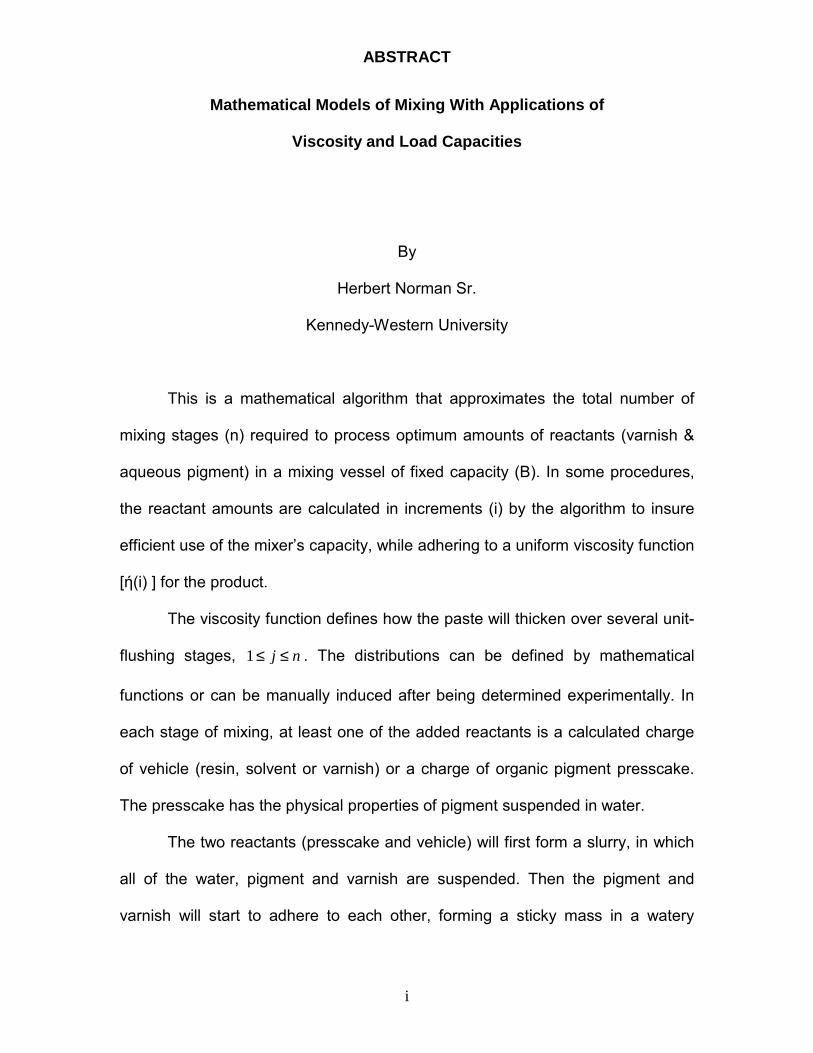
This is a mathematical algorithm that approximates the total number of
mixing stages (n) required to process optimum amounts of reactants (varnish &
aqueous pigment) in a mixing vessel of fixed capacity (B). In some procedures,
the reactant amounts are calculated in increments (i) by the algorithm to insure
efficient use of the mixer�s capacity, while adhering to a uniform viscosity function
[ή(i) ] for the product.
The viscosity function defines how the paste will thicken over several unit-
flushing stages, 1≤ ≤j n . The distributions can be defined by mathematical
functions or can be manually induced after being determined experimentally. In
each stage of mixing, at least one of the added reactants is a calculated charge
of vehicle (resin, solvent or varnish) or a charge of organic pigment presscake.
The presscake has the physical properties of pigment suspended in water.
The two reactants (presscake and vehicle) will first form a slurry, in which
all of the water, pigment and varnish are suspended. Then the pigment and
varnish will start to adhere to each other, forming a sticky mass in a watery

ABSTRACT
ii
environment, thus displacing the water molecules in the aqueous pigment slurry.
The resin and solvent (varnish) particles are more attracted to the pigment
particles than the water, thus wetting the pigment and displacing the water in an
environment where the vehicle the vehicle-to-pigment ratio is greater than one.
The displaced water can be extracted from the system by means of pour-off and
vacuum. The complete process is known as flushing.
The initial objective of this research is to develop general mathematical
models, which will simulate the observed optimized flushing procedures. Given a
minimum of input parameters, the model calculates the flush output parameters
such as the increments of pigment and vehicle charges as generated by the
viscosity distribution function. The results of the research for this thesis led to the
development of three models, which are referred to as Treatments I, II and III. All
three of the models produce feasible outputs, some of which were verified by
processes used on actual manufacturing work orders. Since the simulations are
math models, the procedures can be programmed on a computer. In this thesis,
all source code for programs will be provided and written in QuickBasic. The
procedures will also be modeled in MathCad worksheets.
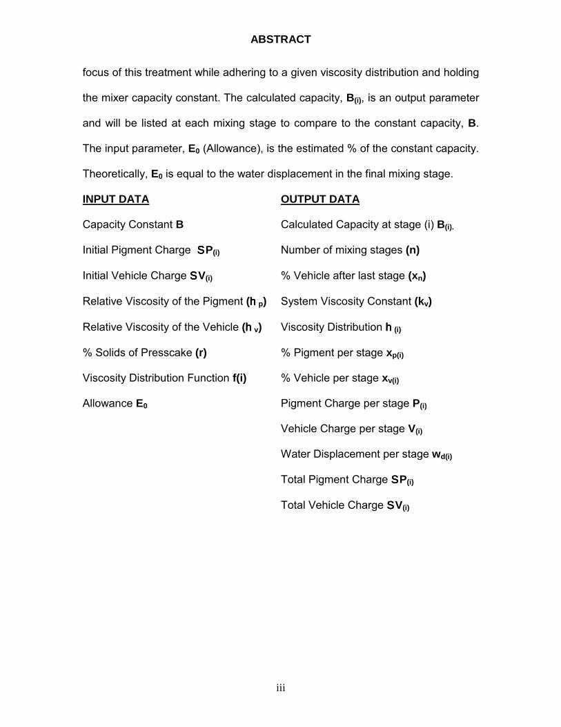
Treatment-I requires initial amounts of pigment and vehicle to be charged to the
mixer. The model calculates the amounts of pigment and vehicle charges that
are required for each mixing stage so that the sum of the increment charges will
equal the optimized total charge. In other words, this model distributes the total
charge to agree with the given viscosity distribution. Optimization is the primary
ABSTRACT
iii
focus of this treatment while adhering to a given viscosity distribution and holding
the mixer capacity constant. The calculated capacity, B(i), is an output parameter
and will be listed at each mixing stage to compare to the constant capacity, B.
The input parameter, E0 (Allowance), is the estimated % of the constant capacity.
Theoretically, E0 is equal to the water displacement in the final mixing stage.
INPUT DATA OUTPUT DATA
Capacity Constant B Calculated Capacity at stage (i) B(i).
Initial Pigment Charge SSSSP(i) Number of mixing stages (n)
Initial Vehicle Charge SSSSV(i) % Vehicle after last stage (xn)
Relative Viscosity of the Pigment (hhhhp) System Viscosity Constant (kv)
Relative Viscosity of the Vehicle (hhhhv) Viscosity Distribution hhhh(i)
% Solids of Presscake (r) % Pigment per stage xp(i)
Viscosity Distribution Function f(i) % Vehicle per stage xv(i)
Allowance E0 Pigment Charge per stage P(i)
Vehicle Charge per stage V(i)
Water Displacement per stage wd(i)
Total Pigment Charge SSSSP(i)
Total Vehicle Charge SSSSV(i)
ABSTRACT
iv
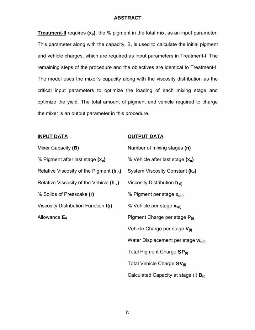
Treatment-II requires (xp), the % pigment in the total mix, as an input parameter.
This parameter along with the capacity, B, is used to calculate the initial pigment
and vehicle charges, which are required as input parameters in Treatment-I. The
remaining steps of the procedure and the objectives are identical to Treatment-I.
The model uses the mixer�s capacity along with the viscosity distribution as the
critical input parameters to optimize the loading of each mixing stage and
optimize the yield. The total amount of pigment and vehicle required to charge
the mixer is an output parameter in this procedure.
INPUT DATA OUTPUT DATA
Mixer Capacity (B) Number of mixing stages (n)
% Pigment after last stage (xp) % Vehicle after last stage (xn)
Relative Viscosity of the Pigment (hhhhp) System Viscosity Constant (kv)
Relative Viscosity of the Vehicle (hhhhv) Viscosity Distribution hhhh(i)
% Solids of Presscake (r) % Pigment per stage xp(i)
Viscosity Distribution Function f(i) % Vehicle per stage xv(i)
Allowance E0 Pigment Charge per stage P(i)
Vehicle Charge per stage V(i)
Water Displacement per stage wd(i)
Total Pigment Charge SSSSP(i)
Total Vehicle Charge SSSSV(i)
Calculated Capacity at stage (i) B(i)

ABSTRACT
v
Treatment-III uses the input parameter, Total Pigment Charge SSSSP(i), to create
the pigment distribution, P(i). In this model, the pigment distribution is a
geometric progression, whose sum is equal to the input total pigment charge,
SSSSP(i). The number of terms in the geometric progression, (n), is treated as the
number of mixing stages in the flush procedure. The viscosity distribution is an
output parameter based on the actual % pigment, xp(i), calculated at each
incremental stage (i). The mixer capacity, B, is held constant through out the
procedure. The calculated capacity B(i), is is an output parameter and will be
listed at each mixing stage to compare to the constant capacity, B. In this
treatment, the allowance, E0, is not required or used.
INPUT DATA OUTPUT DATA
Total Pigment Charge SSSSP(i) Number of mixing stages (n)
Total Vehicle Charge SSSSV(i) % Vehicle after last stage (xn)
Relative Viscosity of the Pigment (hhhhp) System Viscosity Constant (kv)
Relative Viscosity of the Vehicle (hhhhv) Viscosity Distribution hhhh (i)
% Solids of Presscake (r) % Pigment per stage xp(i)
Pigment Distribution Function f(i) % Vehicle per stage xv(i)
In a Geometric Progression model, Pigment Charge per stage P(i)
Capacity B(i) is Constant for all Vehicle Charge per stage V(i)
stages. (1 < i < n) Water Displacement per stage wd(i)
Total Pigment Charge SSSSP(i)
Total Vehicle Charge SSSSV(i)
ABSTRACT
vi
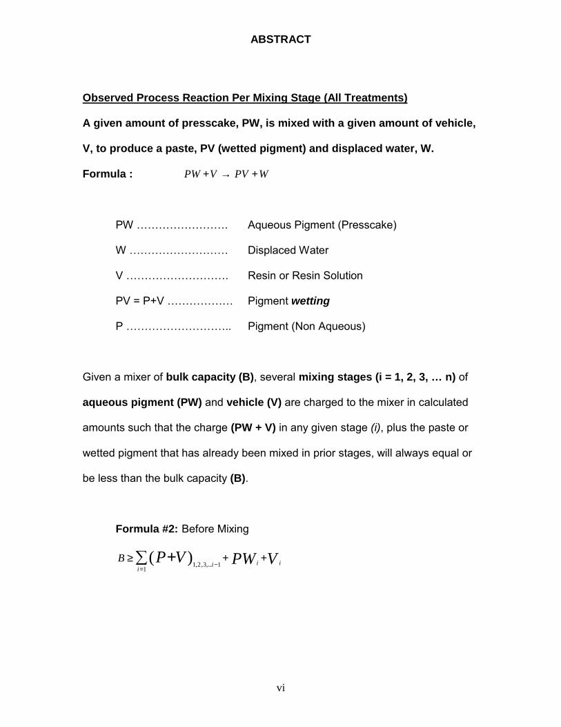
Observed Process Reaction Per Mixing Stage (All Treatments)
A given amount of presscake, PW, is mixed with a given amount of vehicle,
V, to produce a paste, PV (wetted pigment) and displaced water, W.
Formula : PW V PV W+ → +
PW ��������. Aqueous Pigment (Presscake)
W ��������� Displaced Water
V ���������. Resin or Resin Solution
PV = P+V ������ Pigment wetting
P ���������.. Pigment (Non Aqueous)
Given a mixer of bulk capacity (B), several mixing stages (i = 1, 2, 3, … n) of
aqueous pigment (PW) and vehicle (V) are charged to the mixer in calculated
amounts such that the charge (PW + V) in any given stage (i), plus the paste or
wetted pigment that has already been mixed in prior stages, will always equal or
be less than the bulk capacity (B).
Formula #2: Before Mixing
Bi
ii iP V PW V≥ + +
−=
+∑ 1 2 3 11
, , ,...( )

ABSTRACT
vii
Formula #3: After Mixing WPVVP iii
iB ++≥∑ +
=−
11,...3,2,1)(
The discharge of water, (Wi), after any stage of mixing creates the net capacity
for the next stage of additives, (Pi+1 + Vi+1).

LIST OF FIGURES/TABLES
Figure 1.01a Growth Function
Figure 1.01b
LIST OF FIGURES/TABLES
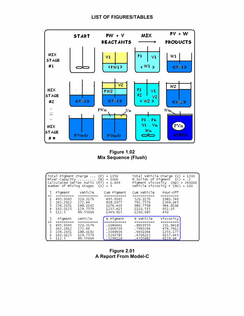
Figure 1.02 Mix Sequence (Flush)
Figure 2.01 A Report From Model-C

LIST OF FIGURES/TABLES
Ball-Mill Formulation Example
%
Pigment 10.0 Stage I (grinding), Then add: Resin 1.0 Solvent 3.0 Resin 1.0 Stage II (let down), Empty mill – then add: Solvent 3.0 Resin 29.0 Stage III (completion of formula) Solvent 51.5 Additives 1.5 100.0
Types of Viscometers
I. Capillary Viscometers Absolute viscometers Relative viscometers
II. Falling Body Viscometers The Falling Sphere Viscometers The Rolling Sphere Viscometers The Falling Coaxial Cylinder Viscometer The Band Viscometer
III. Rotational Viscometers Coaxial Cylinder Viscometer Cone-plate Viscometers
IV. Vibration Viscometers

LIST OF FIGURES/TABLES
Table 1-1: Typical Viscosities and Shears Shear Stress Shear Rate Viscosity . (dynes/cm2) (sec-1) (poises) Emulsion 280 7 40 500 29 17 625 72 9 Vinyl Plastisol 710 36 20 1430 58 25 2130 77 28 Rotation of Fuid Masses – Open Vessels
Proof that the form of the free surface of the liquid in a rotating vessel is that of a paraboloid of revolution. The equation of the parabola is
22
2x
gy ω=
LIST OF FIGURES/TABLES
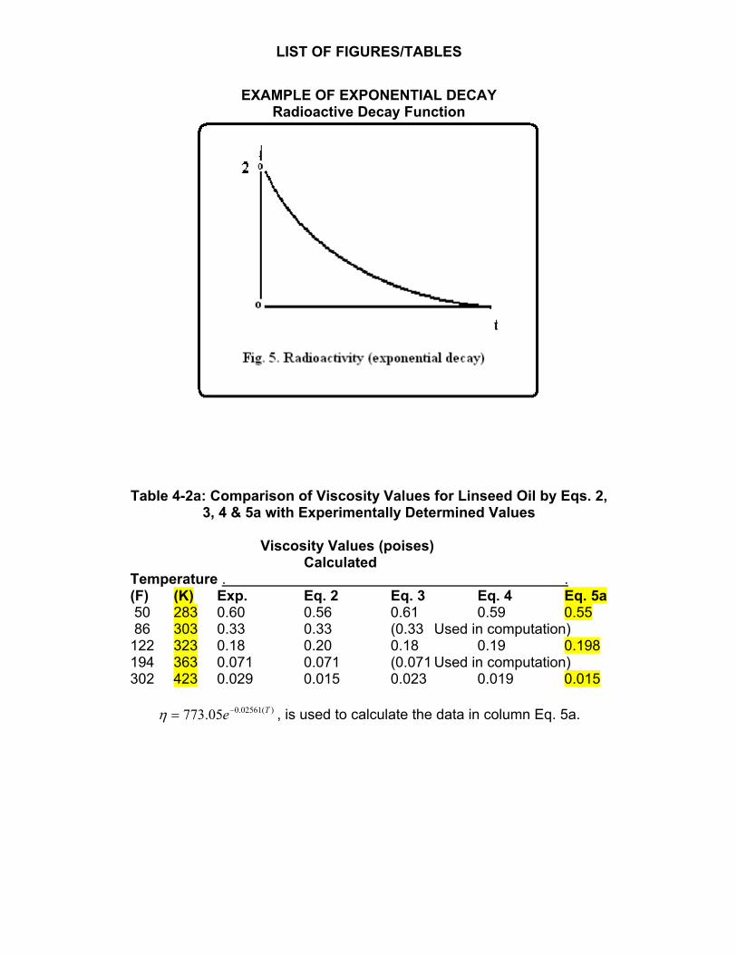
EXAMPLE OF EXPONENTIAL DECAY Radioactive Decay Function
Table 4-2a: Comparison of Viscosity Values for Linseed Oil by Eqs. 2, 3, 4 & 5a with Experimentally Determined Values
Viscosity Values (poises)
Calculated Temperature . . (F) (K) Exp. Eq. 2 Eq. 3 Eq. 4 Eq. 5a 50 283 0.60 0.56 0.61 0.59 0.55 86 303 0.33 0.33 (0.33 Used in computation) 122 323 0.18 0.20 0.18 0.19 0.198 194 363 0.071 0.071 (0.071 Used in computation) 302 423 0.029 0.015 0.023 0.019 0.015
)(02561.005.773 Te−=η , is used to calculate the data in column Eq. 5a.
CHAPTER 1
INTRODUCTION
Statement of the Problem:
Most of the written references on pigment dispersion focus on the
chemistry of organic colorants and the physical chemical properties of the
mixes and suspensions. The flushing process has progressed over the
years from grinding in a mixing vessel to movement through conduits to
complex helical mixing chambers.
The former method involves adding aqueous pigment (presscake)
and oil based vehicles into a sigma-blade mixing vessel over several
stages. The mixing displaces the water from the pigment-presscake and
encapsulates the pigment particles with the oil-based vehicles. The water
is poured off of the pigment dispersion and the cycle is repeated until the
vessel is filled to near capacity. The process is called flushing and it is as
much of an art as it is a science. Process operators modify the procedures
much like a cook uses a recipe. Very few processes are identical. Some
pigment and organic ink manufactures still use this process.
Quantifying this flush process is the primary focus of this project. By
using the above general description of the flushing process, models can
be created to simulate the procedure. These models will use bulk load
capacity and viscosity as the major constraints to produce the number of
Page 1
CHAPTER 1
mixing stages that are required to optimize the quantities of presscake and
vehicle.
There are an infinite number of ways to load the ratio of vehicle to
pigment charges for each addition. The ratio used for each charge, is
usually determined by experimental methods in a laboratory environment.
One of the objectives in this project is to create some models and
methodologies that simulate this experimental process. By using the bulk
load capacity and viscosity as input parameters, these models will
calculate the required quantities of vehicle and pigment needed at each
mixing stage.
Purpose of the Study:
The purpose of this project is to show how the models are created
and used to predict and analyze the viscosities of resin solutions and
pigment dispersions prior to actual mixing. The models are mathematical
functions, which show how temperature, concentrations and other
parameters relate to the flow of end mixed product.
Further development of these models will show how mathematical
logic can be used to simulate and analyze complex mixing procedures
using relative viscosity and mixing capacity. These models will simulate
the paint flow and pigment dispersion dynamics used in industry.
Page 2
CHAPTER 1
Importance of the Study:
The procedure for getting projects from concept to production
works much the same as it did decades ago, except for the upgrades in
plant, lab and computer equipment. Hopefully the system is more
productive and efficient. The need for analysis still remains and is even
more important. The experience of the technologist is just as important
now, if not more so. The procedure that is run in the lab is a model of
expected results in a production environment. The skill set of the
technologist, the quality of the lab equipment used and the quality of the
analysis of the results, will determine how well the lab results correlates to
the production application.
Scope of the Study:
Good models will yield plausible results, which can save time and
resources in development and production. If it is useful, it can be a
valuable tool. The models developed in this project have been created
with Math Cad and Microsoft Excel spreadsheets and will be detailed in
the appendices.
This project will refer to calculated or relative values of viscosity
(poise). In no way is it intended for these values to be interpreted as the
Page 3
CHAPTER 1
absolute viscosity nor the coefficient of viscosity of the dispersion. At best,
the calculated viscosities and yield values are intended to estimate and
quantify the relative thickness of paints, pigments, resins and solutions
with respect to each other.
In this project, the bulk load capacity is the maximum pounds
required to optimize the mixer and produce the desired output. The unit of
measure used for the amounts of vehicle and pigment to be charged to
the mixing vessel will also be pounds.
The treatment of the models uses mathematics, which range from
Summation Algebra to Linear First Order Differential Equations. Most of
the mathematical expressions will be derived from logical statements,
much like postulates and proofs that are used in geometry. The proofs and
derivations, when required, will be detailed in the appendices.
The Rationale of the Study:
A few years ago, the typical industrial coatings development group
consisted of several gifted and creative people with many years of
rheological and analytical backgrounds. Their expertise ranged from the
graphic arts to Ph.D. in Engineering and Chemistry. It has been my
privilege to work with some of these individuals in the pigment
manufacturing and finished ink industry. At that time, microcomputer
Page 4
CHAPTER 1
technology was being introduced into the color and coatings industry. A
typical pigment design problem would have required a senior technical
person to outline or sketch a flush color procedure and assign it to a junior
technician or engineer to work on. The technologist would review the lab
procedure, make the final calculated adjustments and gather the materials
needed to complete the lab procedure. Upon completion of the lab work,
the technologist reviews the results, completes the analysis and returns
the document to the senior technologist.
The primary objective of the methodologies and models that are
created in this project is to emphasize their importance and improve the
quality of the analysis and project management in a laboratory
environment.
More specifically, this project will show how models are created and
used to estimate viscosities of resin solutions. The models are comprised
of mathematical functions, which show how temperature, concentrations
and mixer capacity affect the flow of resin and pigment dispersions.
Further development of these models, show how mathematical
logic is used to simulate and analyze complex mixing procedures using
relative viscosities and mixing capacities. These models simulate the paint
flow and pigment dispersion dynamics that are currently used in industry.
Page 5
CHAPTER 1
Definition of Terms:
Apparent Viscosity
Building up the body with respect to viscosity
Binding The maximum load in pounds a flush mixer will handle. Bulk Capacity Property of certain pigment dispersion systems which causes them to
exhibit an abnormally high resistance to flow when the force which causes them to flow is suddenly increased.
Colloid Dispersions of small particles of one material in another. Dilatant The movement of wetted particles into the body of the liquid or
suspension. Dispersion Same as wetting. Encapsulate The reciprocal of Newtonian viscosity. Unit of measure is (Rhe) Flocculation In the flushing process the moist cakes from the filter press are
introduced into a jacketed kneading type mixer together with the calculated quantity of vehicle. During subsequent mixing, the oil or vehicle displaces the water by preferential wetting, the separated water being drawn off periodically; the final traces of water being removed, when necessary, by heat and partial vacuum. The batch is then sometimes given several grinds through a roller mill to complete the process.
Fluidity The mechanical breakup and separation of the particle clusters to isolated primary particles.
Flushing "True liquid:" A liquid in which the rate of flowis directly proportional to the applied force
Grinding The solid portion of printing inks which impart the characteristics of color, opacity, and to a certain part of the printing ink that is visible to the eye when viewing printed matter.
Newtonian Liquid
A viscous liquid which exhibits Plastic Flow. A liquid that has yield value in addition to viscosity, and a definite finite force must first be applied to the material to overcome the static effect of the yield value before the material may be made to flow.
Oil Absorption The minimum amount of oil or varnish required to “wet” completely a unit weight of pigment of dry color. Raw linseed oil is the reference vehicle in the plant industry, while litho varnish of about twelve poises viscosity (#0 varnish) is the testing vehicle more commonly used in the printing ink industry.
Pigment The moist cakes from the filter press are used in the flush process
Page 6
CHAPTER 1
Plastic Material that has variable fluidity and no yield value. Presscakes The science of plastic flow Pseudoplastic Characteristic of false body or high yield value at rest. Applied aggitation
breaks down the false body to near newtonian flow, but will return to high yield upon standing
Rheology The proportionality constant between a shearing force per unit area (F/A) and velocity gradient (dv/dx).
Thixotropy Wetting refers to the displacement of gases (such as air) or other contaminants (such as water) that are absorbed on the surface of the pigment particle with subsequent attachment of the wetting medium to the pigment surface.
Viscosity The action of a dispersed particles coming back together and forming clusters. As a result, the body builds up thus causing a higher viscosity or yield value.
Wetting The permanent property of an ink that is a measure of its inherent rigidity. It refers to a certain minimum shear stress tha must be exceeded before flow takes place
Yield Value Term used to indicate that the viscosity is that of a non-Newtonian liquid. The adjective apparent is not meant to imply that the viscosity is an illusory value, but rather that the viscosity pertains to only one shear rate condition.
Page 7

CHAPTER 1
OVERVIEW OF THE STUDY
Elementary science and basic chemistry taught us that mater
existed in one of three states; solid, liquid or gas. As we grew older, we
learned that substances exist in physical states, which are none of these
three basic states, but fall somewhere in between. Smoke, molasses,
varnish and paint are examples. P. W. Atkins, Physical Chemistry (1982),
p. 842, a college textbook, defines a colloid as “… dispersions of small
particles of one material in another.”
This project will focus on the methodology and model development
to approximate the flow and general rheological parameters combined
with the load capacities of the mixing vessel using aqueous displacement.
Herbert J. Wolfe, Printing and Litho Inks, (1967), p. 90, describes aqueous
displacement (flushing), “In the flushing process the moist cakes from the
filter press are introduced into a jacketed kneading type mixer together
with the calculated quantity of vehicle. During subsequent mixing, the oil
or vehicle displaces the water by preferential wetting, the separated water
being drawn off periodically; the final traces of water being removed, when
necessary, by heat and partial vacuum. The batch is then sometimes
given several grinds through a roller mill to complete the process.”
Page 8

CHAPTER 1
The part of the above definition, which refers to the “… calculated
quantities of vehicle.”, is the primary focus of this project. Given a
quantity of pigment paste, there are an infinite number of given quantities
of vehicle that can be mixed with the paste, such that the ratio of vehicle to
pigment solids is greater than one. The definition of wetting, according to
Temple C. Patton, Paint Flow and Pigment Dispersion, 1st edition, (1963),
p. 217, “Wetting refers to the displacement of gases (such as air) or other
contaminants (such as water) that are absorbed on the surface of the
pigment particle with subsequent attachment of the wetting medium to the
pigment surface.”
This mixing process is repeated until a mass of flushed pigment,
suspended in vehicles (oils, varnishes and resin). The relative viscosity of
the end product is usually greater than the viscosity or yield value of the
first mixing stage. The first and early mixing stages are usually where
wetting takes place. Vehicle to pigment ratio is at its highest values during
wetting, to maximize the dispersion and encapsulation of the pigment
particles. Wetting is followed by a series of grinding and binding stages,
where the vehicle to pigment ratio is gradually decreased. Sometimes
vehicles of higher relative viscosities are used in these later stages in
order to build the body of the mix.
Page 9

CHAPTER 1
The relative viscosity increases sharply in the early stages and
levels off as the number of mixing stages approaches the final stage (n). A
function that will model the building of the incremental viscosities, (hi),
over the stages, (1≤ i ≤ n), could be an exponential function (1 – ex) or a
logarithmic function, a[ln(x)]. Refer to Figure 1.01 below.
Figure 1.01a
Figure 1.01b
Page 10

CHAPTER 1
In theory, there is no limit to the number of mixing stages that could
be used, but in reality, mixing capacity and the capacity to mix, is one the
key parameters, which implies a logical end point to stop the process.
Given a beaker and a spatula as the mixing utility, the capacity (B),
of the beaker and the ability to apply shear to the mixture of paste and
vehicles, tends to identify the some of the practical limits of the process.
The contents of the beaker and the energy required to mix the vehicle and
displace the water, should not exceed the beaker volume of the mixing
unit and cause overflow. Once the water is squeezed from the sticky mass
of wetted pigment, the water is discarded.
If the beaker volume is optimized prior to mixing, the new volume
for the next addition is equal to the volume of water discarded. This mixing
cycle is repeated until the working capacity of the mixer is reached and
there is no more room to mix without overflow. The number of mixing
stages (n) required to flush (P) amount of pigment is also determined
experimentally and is one of the parameters that will be used in this
project. For the sake of symbolic variables, (PW) will be assigned to
aqueous pigment paste, since it is composed of pigment, (P), and water,
(W). The variable assigned to vehicle is (V). The colloidal suspension or
pigment dispersion is assigned the variable (PV). Refer to Figure 1.02
below.
Page 11

CHAPTER 1
Figure 1.02 (Flush Sequence)
The general mixing reaction equation is expressed as follows:
Formula #1: PW + V = PV + W
Given a mixer of capacity (B), several increments (n) of aqueous pigment
(PW), and vehicle (V), are charged to the mixer in amounts such that the
incremental charge (PW + V), will not overflow the mixer vessel. At the
end of each mixing stage, the water (W), becomes insoluble in the mixture
(PV + W), and is discharged from the vessel leaving only a sticky mass of
pigment dispersed in the vehicle (PV).
Page 12
CHAPTER 1
Formula #2: Before Mixing: ∑−
=
+++≥1
1)(
i
iiii VPWVPB
Formula #3: After Mixing: ∑−
=
+++≥1
1)(
i
iiii WPVVPB
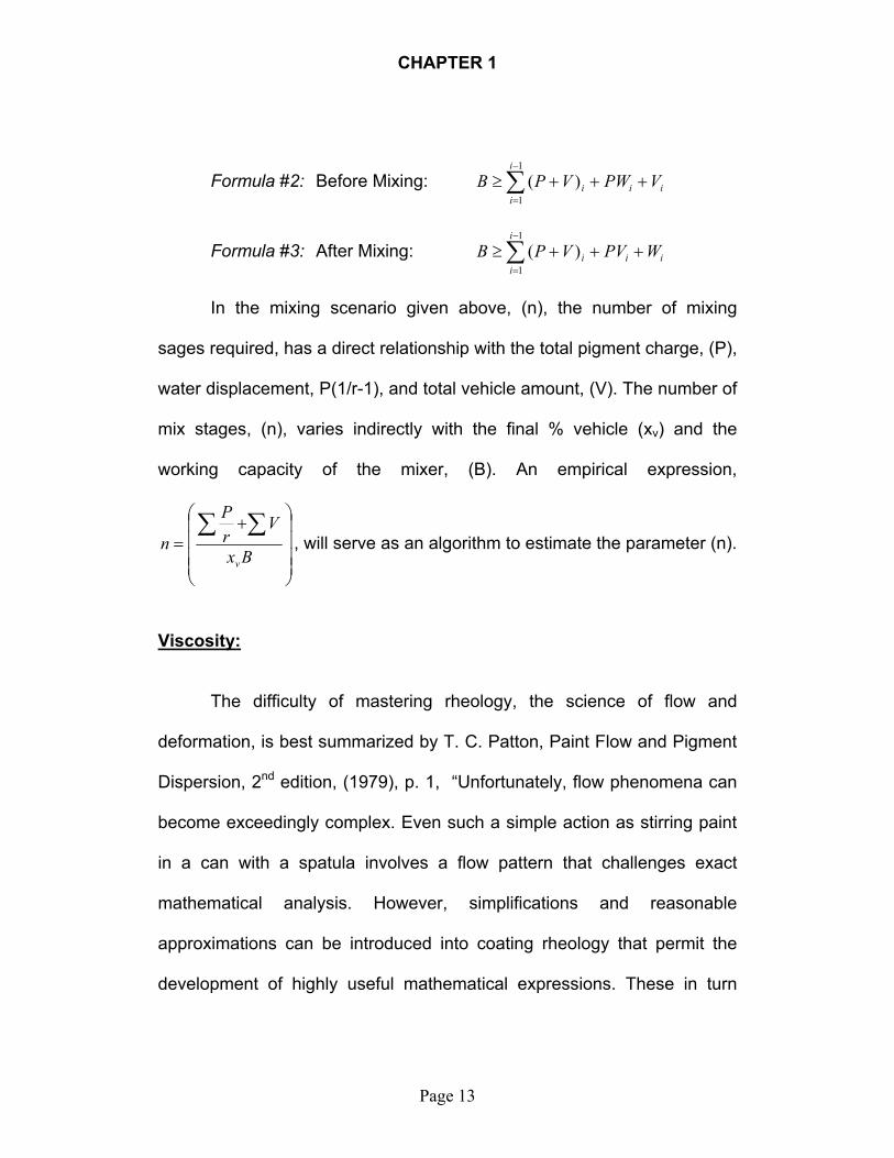
In the mixing scenario given above, (n), the number of mixing
sages required, has a direct relationship with the total pigment charge, (P),
water displacement, P(1/r-1), and total vehicle amount, (V). The number of
mix stages, (n), varies indirectly with the final % vehicle (xv) and the
working capacity of the mixer, (B). An empirical expression,
+=
∑∑Bx
VrP
nv
, will serve as an algorithm to estimate the parameter (n).
Viscosity:
The difficulty of mastering rheology, the science of flow and
deformation, is best summarized by T. C. Patton, Paint Flow and Pigment
Dispersion, 2nd edition, (1979), p. 1, “Unfortunately, flow phenomena can
become exceedingly complex. Even such a simple action as stirring paint
in a can with a spatula involves a flow pattern that challenges exact
mathematical analysis. However, simplifications and reasonable
approximations can be introduced into coating rheology that permit the
development of highly useful mathematical expressions. These in turn
Page 13

CHAPTER 1
allow the ink or paint engineer to proceed with confidence in controlling
and predicting the flow performance of inks or paint coatings.”
Viscosity is defined as the opposition to fluidity. Water passes
through a funnel quickly; boiled oil slowly, while treacle would pass
through very slowly. An explanation for such varied rates of liquid
movement is as follows. When a liquid is caused to move, a resistance to
the motion, is set up between adjacent layers of the liquid, just as when a
block of wood is dragged along the floor. In the latter case, friction arises
between the two solid surfaces; in the case of a liquid, friction arises
between moving surfaces within it. This internal friction is called viscosity.
The frictional force, which opposes motion is felt when one moves a hand
through a tub of water. All liquids show a resistance to flow. Although
forces applied externally, affect the rate of liquid flow, viscosity is
concerned only with the internal frictional effect.
If two layers of a liquid are moving at different speeds the faster
moving layer experiences resistance to its motion, while the slower
moving layer experiences a force which increases its velocity. The
coefficient of viscosity is defined as the force in dynes required per square
centimeter to maintain a difference in velocity of 1 cm/sec between two
parallel layers of the fluid, which are ( d∆ ), 1 cm apart. This is best
represented in the following expression from James F. Shackelford,
Page 14

CHAPTER 1
Introduction to Materials Science for Engineers, (1985), p.329, vadf
∆∆
=η ,
where (η ) is the coefficient of viscosity in poise, ( ) is the area in cma 2,
( ν∆ ) is change in velocity in cm/sec and ( ) is the applied force in dynes. f
shearofratestress
__
f
=η
The liquids for whose rate of flow varies directly with the applied
force ( ), are called Newtonian Liquids. However, Non-Newtonian flow
is observed when the dispersed molecules are elongated, when there are
strong attractions between them or when dissolved or suspended matter is
present, as in resin and paint solutions. Most paint and pigment solutions
show Non-Newtonian viscosity to some degree.
Newtonian (Simple Flow):
An ideal liquid having a constant viscosity at any given temperature for low
to moderate shear rates.
Page 15

CHAPTER 1
Non-Newtonian (Plastic Flow):
Flow with a yield value. This is a minimum shear stress value that must be
exceeded before flow will take place. Below yield value, the substance has
elastic properties. (Pigment-Resin-Solvent Solutions.)
Non-Newtonian (Pseudoplastic Flow):
A hybrid flow, which simulates plastic flow at moderate to high shear rates,
and Newtonian flow at low shear rates. (Paint and Ink Solutions.)
Non-Newtonian (Dilatant Flow):
Viscosity is reduced as shear stress is increased. This type of solution
gets thicker on increased agitation. (Rare Paint Systems)
Non-Newtonian (Thixotropic Flow):
Much like Pseudoplastic flow, but more complex and plasticized. In
general, thixotropic breakdown (loss of viscosity) is fostered by an
increase in the shear stress, by prolonging the shear time. When the
shear stress is removed, recovery of thixotropic viscosity ensues as
thixotropic structure is again built up throughout the paint system.
Page 16

CHAPTER 1
Dispersions:
As a vehicle is incorporated with pigment by a mixing action, a
good dispersion initially displays significant resistance to sudden pressure,
turning dull in appearance. With further vehicle addition, the mixture
reaches a point where it coalesces into a smooth glossy mass. A small
additional increment of vehicle converts the mass into a mobile dilatant
dispersion.
Physically, this dispersion is characterized by deflocculated
particles, fully separated by a minimum of dispersion vehicle to give a
relatively closely packed system. If the shear stress applied to this
dispersion is low, sufficient time is allowed for the particles to slip and slide
around each other without contact. As a result of this action, a minimum
viscosity resistance results. If the shear stress is high, then adjacent
particles ram through the mix barrier separating themselves to establish
solid-to-solid contact. Without the lubrication afforded by the intervening
dispersion vehicle, major viscous resistance is exhibited.
Besides mixing the vehicle with the pigment particles, there is
another phenomena taking place which affects the body and consistency
of the dispersion. This action is absorption. The amount of absorption that
takes place depends on the interactive properties of the surface of the
pigment and the properties of the vehicle. The absorption causes some
Page 17
CHAPTER 1
puffiness about the surface of the pigment particles and thus the same is
observed on a larger sampled mass. This puffiness causes a slight build
up in viscosity of the dispersion and also contributes to the flocculation.
The above properties will provide the basic resource for
constructing the logic and math models to simulate the flushing process.
Page 18

CHAPTER 2
REVIEW OF RELATED LITERATURE
Paint Technology Manuals
PART TWO – Solvents, Oils, Resins and Driers
Published on behalf of The Oil & Colour Chemists’ Association – 1961
This manual covers the chemistry and physical chemical
characteristics of oils and resins. The book was very popular with
technologists in the coatings industry because it covered the chemical
derivations and practical applications with regard to paint manufacturing
and ink making. Regarding this project, it was a very useful resource for
information on resins and solvents.
Sometimes the technologist encounters significant chemical
reactions when mixing certain resin solutions such as driers. Without
taking into account the basic chemistry of solvents and resins, one might
assume that just mixing some oil with resin, a varnish like substance will
result. And by adding more oil or solvent to the mix, one would expect the
result to be a thinner solution, which should flow more easily. But what if
there is a reaction with the oxygen in the air, solvent and the resin and the
mix begins to thicken. This is what happens when a drier is created.
Page 19
CHAPTER 2
Coatings of all resin solutions have a tendency to dry because of a
chemical process called oxidation. But what categorizes a resin solution
as a drier is the relative rate of drying, resin concentration and sometimes
temperature.
“Paints have been made for centuries by mixing pigments such as
red lead, white lead and umber with drying oils, and it became
obvious that these paints dried faster than the raw oils. Eventually it
was discovered that oils stored in the presence of lead or
manganese compounds, e.g. red lead or manganese dioxide, or
better still if heated in the presence of these compounds so as to
produce oil-soluble products, developed improved drying
properties; this formed the basis of the production of boiled linseed
oil; one of the foundations of paint formulation. “ (Atherton, 1961, p.
31)
Drying is just one of the many challenges that a coating technologist will
encounter. Because of various degrees of chemical reactions, there are
numerous levels of compatibility of solvents, resins and pigments. Today
these dispersions are classified into solvent and resin systems.
This project employs non-drying dispersions, which will allow
wetting to take place without rapid oxidation and aggregation. The mixing
Page 20
CHAPTER 2
methodology assumes ideal systems of resins and solvents. This manual
on resins and solvents gave me a great appreciation on the complexity
and sophistication of the behavior of pigment and resin dispersions. There
is much room for further development of this mixing model using non-
idealistic resin solutions as vehicles. The ink chemistry and physics
involved in the actual rheology of pigment dispersions go far beyond the
level of mathematics used in this project.
Page 21

CHAPTER 2
Introduction to Paint Chemistry
By G. P. A. Turner - 1967
Turner’s treatment of paint chemistry is somewhat of a general
treatment of the physics and chemistry of paint. It reviews the inorganic
and organic systems of paint chemistry. Turner also incorporates some of
the information that was previously covered on oils, solvents, resins and
driers. This book on paint chemistry is more of a general textbook on the
manufacturing and production of paint. It covers general atomic theory as
it relates to molecular bonding of compounds used in paint. He discusses
viscosity of suspensions and colloids. There is an introduction to
substrates and color theory, where the science of polymer coating is
explained quite clearly.
The chapter on pigmentation describes the dough mixer, which are
used by many pigment manufactures to produce distributions.
“A fourth type of mill is the heavy duty or ,‘pug’ mixer, in which
roughly S-shaped blades revolve in opposite directions and at
different speeds in adjacent troughs. A stiff paste is required.
Several alternative mills are available, which the reader may
discover elsewhere.” (Turner, 1967, p. 119)
Page 22

CHAPTER 2
The dough mixers mentioned above is an accurate description of the
mixing vessels used in processing flush-color dispersions. The S-shaped
blades are called sigma blades. The paint mixing procedure is much like
the flush procedure. The primary stages and their functions are described
as follows.
“It is obvious from the mention of stiff pastes that the whole paint is not
charged into the mill. In fact, the paint maker aims to put in the
maximum amount of pigment of pigment and the minimum amount of
varnish to get the largest possible paint yield from his mill. This
mixture forms the grinding or first stage. When the dispersion is
complete (after a period varying from10 minutes to 48 hours according
to the materials and machinery involved), the consistency is reduced
with further resin solution or solvent, so that the mill can be emptied as
cleanly as possible. This is the ‘let-down’ or second stage and may
take up two hours. The third or final stage (carried out in a mixing
tank) consists of the completion of the formula by addition of the
remaining ingredients. A break-down of a possible ball mill formula
looks like this:
Page 23

CHAPTER 2
%
Pigment 10.0 Stage I (grinding), Then add:
Resin 1.0
Solvent 3.0
Resin 1.0 Stage II (let down), Empty mill – then add:
Solvent 3.0
Resin 29.0 Stage III (completion of formula)
Solvent 51.5
Additives 1.5
100.0
The exact composition of Stage I is found by experiment, to give the
minimum grinding time and the most stable and complete dispersion.
Stages II and III also require care, as hasty additions in an incorrect
order can cause the pigment to re-aggregate (flocculate).
The amount of pigment in the formula is that required for the
appropriate colour, hiding power, gloss, consistency and durability. As
a rough guide, the amount might vary from one third of the binder
weight to an equal weight (for a glossy pastel shade).” (Turner, 1967,
p. 119)
Page 24
CHAPTER 2
The above procedure is very much like the total flush procedure. This
project is focused on the referenced grinding Stage I where the pigment is
introduced into the system. In flushing, several stages are required to
introduce all of the pigment into the system. The first stage of the series of
grinding stages is called the wetting stage. In the wetting stage of flushing,
usually the largest charge of pigment and vehicle is introduced to the
mixer, where the vehicle charge is greater than the pigment. The purpose
for the vehicle-to-pigment ratio being greater than one is to allow for the
encapsulation of the pigment particles and maximum displacement of
water. A low viscosity, due to the large amount of vehicle present,
generally characterizes the wetting stage.
The subsequent stages are grinding stages, where the rest of the
pigment is charged to the mixer in lesser amounts. The vehicle-to-pigment
ratio for these stages is usually less than one. A graph of the viscosity of
the dispersion with respect to the number of stages, usually looks similar
to an exponential growth function. Refer to Figures 1.01a and 1.01b.
The 10.0% of pigment in the total paint dispersion shown above is
71.4% of Stage I. In flush procedures after the last stage of pigment
charge, the percent pigment is usually in the range of 50% to 60%.
Page 25
CHAPTER 2
Ferranti Instrument Manual
The Measurement and Control of Viscosity
And Related Flow Properties
McKennell, R., Ferranti Ltd., Moston & Mancheser (1960)
The Ferranti Instrument Manual was written to give the ink
technician an overview of the complexity of measuring viscosity. The
manual lists four major types of viscometers and some examples of each.
Several types of non-Newtonian fluids are discussed. Different types of
non-Newtonian measurements are exemplified and matched with the best
type of viscometer. There are suggestions and examples of experimental
techniques for measuring various types of non-Newtonian substances for
experimental purposes as well as calibration.
A brief overview is given of how viscometers generate automatic
flow-curve recordings and the curves are analyzed. Basic viscosity
formulae are listed and discussed. Specific flow problems and suggested
solutions are discussed.
The list of the four major types of viscometers is listed below. It is
taken from the table of contents of the manual.
Page 26
CHAPTER 2
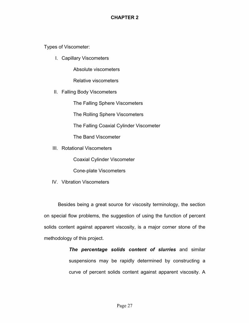
Types of Viscometer:
I. Capillary Viscometers
Absolute viscometers
Relative viscometers
II. Falling Body Viscometers
The Falling Sphere Viscometers
The Rolling Sphere Viscometers
The Falling Coaxial Cylinder Viscometer
The Band Viscometer
III. Rotational Viscometers
Coaxial Cylinder Viscometer
Cone-plate Viscometers
IV. Vibration Viscometers
Besides being a great source for viscosity terminology, the section
on special flow problems, the suggestion of using the function of percent
solids content against apparent viscosity, is a major corner stone of the
methodology of this project.
The percentage solids content of slurries and similar
suspensions may be rapidly determined by constructing a
curve of percent solids content against apparent viscosity. A
Page 27

CHAPTER 2
suitable shear rate must be chosen and adopted as standard
and equilibrium apparent viscosity readings taken on a number
of slurries of known percentage solids content. Determination
can be made in a fraction of the time required using
conventional gravimetric techniques, with an accuracy which is
acceptable for many applications. (Ferranti and McKennell,
1955, “Liquid Flow Problems and Their Solution”: Reprint from
Chemical Product)
Figure 2.01 is a report that was generated from one of the computer
programs written by the author for this project. It shows how percent
content is compared to apparent viscosity can be used as part of the flush
dispersion analysis.
Figure 2.01
A Report From Model-C
Page 28

CHAPTER 2
Paint Flow and Pigment Dispersion
Patton, T. C., 1st edition (1963) & 2nd edition (1979)
Patton takes more of a mathematical approach to explore the
dynamic properties of resin and pigment dispersions. Both editions
provide a practical and comprehensive overview of rheological aspects of
paint and coatings technology. The second edition includes expanded
material on pigment-binder geometry, the theoretical aspects of
dispersion; and a more detailed breakdown of grinding equipment.
The sections that are most referenced for this project are the ones
which elaborate on viscosity, the effects of temperature and resin
concentration on viscosity and pigment dispersion theory.
Viscosity
The treatment of viscosity theory is the same as the other resources.
Patton uses tables which lists various substances and their viscosities to
help the reader better understand the concept of flow. He also uses tables
to show how well viscosity formulae correlate to actual experimental data.
The models in this project will also use tables. I considered this illustrative
technique to be very effective especially in showing results for analysis.
Page 29
CHAPTER 2
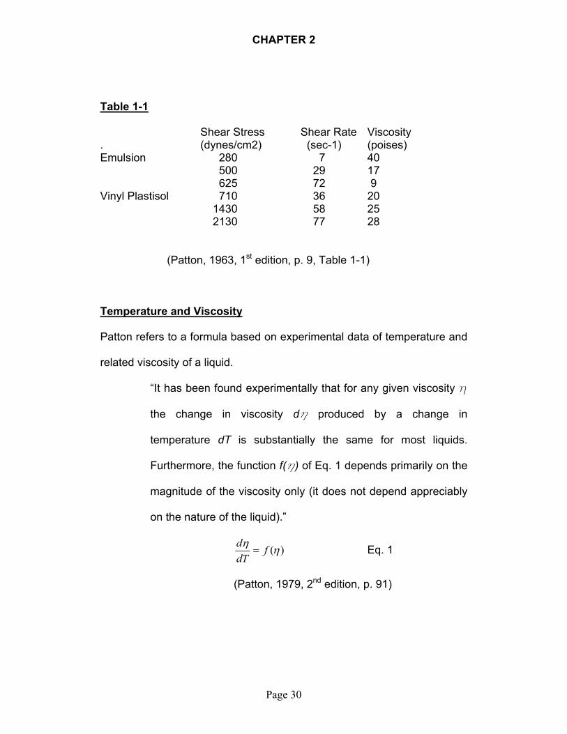
Table 1-1 Shear Stress Shear Rate Viscosity . (dynes/cm2) (sec-1) (poises) Emulsion 280 7 40 500 29 17 625 72 9 Vinyl Plastisol 710 36 20 1430 58 25 2130 77 28
(Patton, 1963, 1st edition, p. 9, Table 1-1)
Temperature and Viscosity
Patton refers to a formula based on experimental data of temperature and
related viscosity of a liquid.
“It has been found experimentally that for any given viscosity h
the change in viscosity dh produced by a change in
temperature dT is substantially the same for most liquids.
Furthermore, the function f(h) of Eq. 1 depends primarily on the
magnitude of the viscosity only (it does not depend appreciably
on the nature of the liquid).”
)(ηη fdTd
= Eq. 1
(Patton, 1979, 2nd edition, p. 91)
Page 30

CHAPTER 2
“Of the many equations that have been proposed for relating
viscosity to temperature, one appears to represent the
viscosity/temperature relationship most accurately. It is commonly
referred to as Andrade’s equation (Eq. 2).
TBA /10(=η Eq. 2
Equation 2 can be expressed alternatively in logarithmic form as Eq. 3.
TBA += logηlog Eq. 3
Temperature T must be expressed in absolute units (K = 273 + C or
R = 460 + F), and A and B are constants for the liquid in question.
If subscripts 1 and 2 are used to denote the conditions for two
different temperatures, it can be readily shown (by subtraction) that the
two conditions are related by Eq. 4.”
)11(log212
1
TTB −=
ηη Eq. 4
(Patton, 1979, 2nd edition, p. 93)
The following table shows how temperature effects the viscosity of linseed
oil and also how well the above equations fit actual experimental data.
This table will also serve as a resource to measure the accuracy of the
formulae and models which will be developed in this project.
Page 31

CHAPTER 2
Table 4-2: Comparison of Viscosity Values for Linseed Oil by Eqs. 2,
3 & 4 with Experimentally Determined Values
Viscosity Values (poises) Calculated
Temperature . . (F) Exp. Eq. 2 Eq. 3 Eq. 4 50 0.60 0.56 0.61 0.59 86 0.33 0.33 (0.33 Used in computation) 122 0.18 0.20 0.18 0.19 194 0.071 0.071 (0.071 Used in computation) 302 0.029 0.015 0.023 0.019
(Patton, 1979, 1st edition, p. 85, Table 4-2)
Resin Concentration
“A common viscosity problem calls for calculating the change in a solution
viscosity produced by a change in resin concentration. Such a change
may be due to addition of let-down thinner, or it may occur as a result of
blending together two compatible resin solutions.” (Patton, 1979, 1st
edition, p. 88)
Equations Relating Viscosity to Resin Concentration
“The simplest expression and possibly a fully adequate one for most
purposes for relating solution viscosity to resin concentration takes the
Page 32

CHAPTER 2
form of Eq. 9, where x is the fractional content of nonvolatile resin in the
resin solution and A and B are constants.
)10( BxA=η or BxA += loglogη Eq. 9
To evaluate the constants A and B, solution viscosities at two different
resin concentrations must be known. Once A and B are determined, a
viscosity for any third resin concentration is obtained by straightforward
substitution in Eq. 9.” (Patton, 1979, 1st edition, p. 88)
The data in the above tables will be referenced in later chapters to
illustrate how other methodologies compare for accuracy and use in
several models. Patton uses logarithms to the base-10 in the above
methodologies. The formulae that will be used in the development of the
flush models will use logarithms to the base-e or natural logs.
Page 33
CHAPTER 2
Printing and Litho Inks
Wolfe, H. J. (1967)
Printing and Litho Inks blends the history and art of ink making with
the world of science and technology. It is the source of many ink-making
terms that are used in this project. Flushing is described as follows.
“As is well known, the kneading type of mixer also is employed in the
“flushing” of pulp colors, i.e., the production of pigment-in-oil pastes
directly from pigment-in-water pastes, by introducing the water-pulp
color and the varnish into the mixer and agitating until the varnish has
displaced the water. Steam-jacketed mixers are generally employed
for this purpose. Air-tight covers also may be fitted to these mixers so
that vacuum may be employed to remove the water from the pulp
more rapidly.” (Wolfe, 1967, p. 445)
The viscosity of the dispersion, relative particle size and oil absorption of
the pigment are very important characteristics that help determine the
point at which to stop mixing. Wolfe provides tables and details about the
properties of the different classes and types of pigment in dry color state.
These dry properties directly relate to the flush procedure (pigment
suspended in water) because the resulting dispersion after displacing the
water (flushing), will have the same properties as if it were mixed dry. If
Page 34

CHAPTER 2
the pigment particle size and the vehicles are the same, then the end
result should be the same. The only difference will be the grinding
methods. Regarding pigments, resins and solvents, Wolfe lists standard
testing procedures, test equipment and test methods used in the printing
ink industry. For example:
The term “oil absorption” as used in the dry color and printing ink
industries refers to the minimum amount of oil or varnish required to
“wet” completely a unit weight of pigment of dry color. Raw linseed oil
is the reference vehicle in the plant industry, while litho varnish of
about twelve poises viscosity (#0 varnish) is the testing vehicle more
commonly used in the printing ink industry. (Wolfe, 1967, p. 472)
Viscosity is without a doubt, the most important characteristic of a printing
ink vehicle, since it determines the length, tack and fluidity of the vehicle;
which in turn in a large measure, determines the working qualities of the
resulting inks. Although listed separately, the properties of viscosity are
directly related to those of oil absorption and particle size. These three
topics are key to the flush models developed in this project.
Page 35
CHAPTER 2
Physical Chemistry
Atkins, P. W. (1982)
The concepts of suspensions and viscosity are covered quite
extensively in physical chemistry. To get more clarification on these terms,
Atkins’ “Physical Chemistry” is a good resource. For example:
“A major characteristic of liquids is their ability to flow. Highly viscous
liquids, such as glass and molten polymers, flow very slowly because
their large molecules get entangled. Mobile liquids like benzene have
low viscosities. Water has a higher viscosity than benzene because its
molecules bond together more strongly and this hinders the flow.
We can expect viscosities to decrease with increasing
temperatures because the molecules then move more energetically
and can escape from their neighbors more easily. (Atkins, 1982, p.18)
Regarding the relationship of viscosity to particle size as stated
above in Wolfe, Atkins confirms this as follows:
The presence of macromolecules affects the viscosity of the
medium, and so its measurement can be expected to give
information about size and shape. The effect is large even at low
concentrations, because the big molecules affect the surrounding
fluid’s flow over a long range.” (Atkins, 1982, p.825)
Page 36
CHAPTER 2
Fluid Mechanics and Hydraulics
Giles, R. V. (June, 1962)
Fluid mechanics and hydraulics explained the viscosity in such an
abstract manner that it was somewhat limited as a resource in this project.
However, the viscosity units of measure were clearly explained and came
in very handy when the property of density was introduced.
Absolute or Dynamic Viscosity (m)
Viscosity of a fluid is that property which determines the amount of
its resistance to a shearing force. Viscosity is due primarily to
interaction between fluid molecules. (Poise, lb-sec/ft2)
Kinematic Viscosity (n)
Kinematic coefficient of viscosity is defined as the ratio of absolute
viscosity to that of mass density (r). (Stokes, ft2/sec = m/r)
(Giles, 1962, p.3)
Page 37

CHAPTER 2
Rotation of Fuid Masses – Open Vessels
The form of the free surface of the liquid in a rotating vessel is that
of a paraboloid of revolution. Any vertical plane through the axis of
rotation which cuts the fluid will produce a parabola. The equation
of the parabola is, 22
2x
gy ω= where x and y are coordinates, in feet,
of any point in the surface measured from the vertex in the axis of
revolution and w is the constant angular velocity in rad/sec. Proof
of this equation is given in Problem 7. (Giles, 1962, p.42)
Problem 7. An open vessel partly filled with a liquid rotates about a vertical axis at constant angular velocity. Determine the equation of the free surface of the liquid after it has acquired the same angular velocity as the vessel.
Page 38
CHAPTER 2
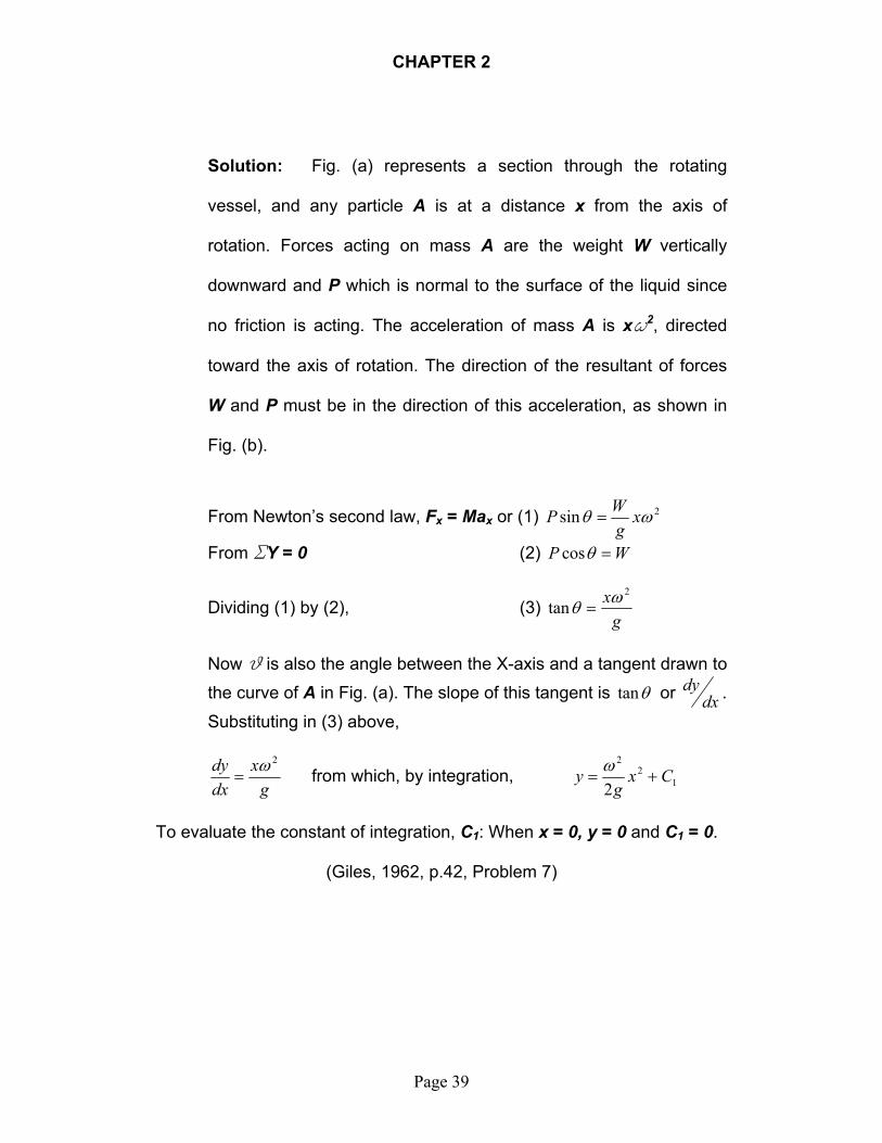
Solution: Fig. (a) represents a section through the rotating
vessel, and any particle A is at a distance x from the axis of
rotation. Forces acting on mass A are the weight W vertically
downward and P which is normal to the surface of the liquid since
no friction is acting. The acceleration of mass A is xw2, directed
toward the axis of rotation. The direction of the resultant of forces
W and P must be in the direction of this acceleration, as shown in
Fig. (b).
From Newton’s second law, Fx = Max or (1) 2sin ωθ xgWP =
From SY = 0 (2) P W=θcos
Dividing (1) by (2), (3) gx 2ωθ =tan
Now q is also the angle between the X-axis and a tangent drawn to
the curve of A in Fig. (a). The slope of this tangent is θtan or dxdy .
Substituting in (3) above,
gx
dxdy 2ω
= from which, by integration, 12
2
2Cx
gy +=
ω
To evaluate the constant of integration, C1: When x = 0, y = 0 and C1 = 0.
(Giles, 1962, p.42, Problem 7)
Page 39

CHAPTER 2
Manual of Chemical Engineering Calculations & Shortcuts
New Analysis Provides Formula to Solve Mixing Problems
Brothman, A, Wollan, G, & Feldman, S. (1947)
Universally used by the process industries, mixing operations have
been the subject of considerable study and research for several years.
Despite these efforts, mixing has remained an empirical art with little
foundation of scientific analysis as found in other important unit
operations. A new approach based on a study of kinetics and on the
concept that mixing is essentially an operation of three-dimensional
shuffling, has resulted in a formula for solving practical problems.
“Mixing is that unit operation in which energy is applied to a mass of
material for the purpose of altering the initial particle arrangement so
as to effect a more desirable particle arrangement. While the object of
this treatment is usually to blend two or more materials into a more
homogenous mixture, it may also serve to promote accompanying
reactions, or it may support other unit operations such as heat
transfer.” (Brothman, Wollan and Feldman, 1947, p.175)
Page 40
CHAPTER 2
The above referenced chapter is about applications of analytical
methods, which brings forth a new relationship between mixing time and
mixing completion. Based on the theory of probability and resulting from a
study of mixing kinetics, the derived expression and its implications may
well lead the way to closer and more reliable correlation of mechanical
design and functional performance of mixers. The concepts and mixing
methodologies are explained in shuffling operation, blending, turbulence
and liquid mixing. Most of the concepts and methodologies referenced in
this book included the mixing time.
After careful consideration, the author decided to omit these
methodologies from this book because their complexity was beyond the
scope of this project. However, the time of mixing, though not used directly
in my models, will have an indirect correlation to the algorithm that will be
used to estimate number of mixing stages required. These mixing
concepts related to functions that are continuous, where my models are
more mathematically discrete.
Page 41
CHAPTER 2
Advanced Engineering Mathematics
Kreyszig, E. (August 1988)
Modeling Physical Applications
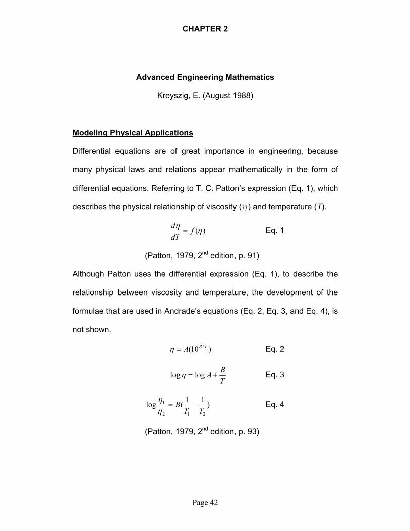
Differential equations are of great importance in engineering, because
many physical laws and relations appear mathematically in the form of
differential equations. Referring to T. C. Patton’s expression (Eq. 1), which
describes the physical relationship of viscosity (h) and temperature (T).
)(ηη fdTd
= Eq. 1
(Patton, 1979, 2nd edition, p. 91)
Although Patton uses the differential expression (Eq. 1), to describe the
relationship between viscosity and temperature, the development of the
formulae that are used in Andrade’s equations (Eq. 2, Eq. 3, and Eq. 4), is
not shown.
)10( /TBA=η Eq. 2
TBA += logηlog Eq. 3
)11(log212
1
TTB −=
ηη Eq. 4
(Patton, 1979, 2nd edition, p. 93)
Page 42

CHAPTER 2
Kreyszig describes the development process in a detailed step by step
example of a radioactive decay problem below.
EXAMPLE 5. Radioactivity, exponential decay
Experiments show that a radioactive substance decomposes at a rate
proportional to the amount present. Starting with a given amount of
substance, say, 2 grams, at a certain time, say, t = 0, what can be
said about the amount available at a later time?
Solution. 1st Step. Setting up a mathematical model (a differential
equation) of the physical process.
We denote by y(t) the amount of substance still present at time t. the
rate of change is dy/dt. According to the physical law governing the
process of radiation, dy/dt is proportional to y.
(9) kydtdy
=
Here k is a definite physical constant whose numerical value is known
for various radioactive substances. (For example, in the case of
radium 88Ra226 we have k ~ -1.4 x 10⁻¹¹ sec-1.) Clearly, since the
amount of substance is positive and decreases with time, dy/dt is
negative, and so is k. We see that the physical process under
Page 43

CHAPTER 2
consideration is described mathematically by an ordinary differentia
equation of the first order. Hence this equation is the mathematical
model of that process. Whenever a physical law involves a rate of
change of a function, such as velocity, acceleration, etc., it will
lead to a differential equation. For this reason differentia
equations occur frequently in physics and engineering.
2nd Step. Solving the differential equation. At this early stage of our
discussion no systematic method for solving (9) is at our disposal.
However, (9) tells us that if there is a solution y(t), its derivative must
be proportional to y. From calculus we remember that exponential
functions have this property. In fact the function ekt or more generally
(10) ktcety =)(
where c is any constant, is a solution of (9) for all t, as can readily be
verified by substituting (10) into (9). [We shall see later (in Sec. 1.2)
that (10) includes all solutions of (9); that is (9) does not have singular
solutions.]
3rd Step. Determination of a particular solution. It is clear that our
physical process has a unique behavior. Hence we can expect that by
using further given information we shall be able to select a definite
Page 44

CHAPTER 2
numerical value of c in (10) so that the resulting particular solution will
describe the process properly. The amount of substance y(t) still
present at time t will depend on the initial amount of substance given.
This amount is 2 grams at t = 0. Hence we have to specify the value
of c so that y = 2 when t = 0. This condition is called an initial
condition, since it refers to the initial state of the physical system. By
inserting this condition
(11) 2)0( =y
in (10) we obtain
y(0) = ce0 = 2 or c = 2
If we use this value of c, then the solution (10) takes the particular form
(12) ktety 2)( =
Page 45

CHAPTER 2
This particular solution of (9) characterizes the amount of substance
still present at any time . The physical constant k is negative, and
y(t) decreases, as shown in Fig. 5.
0≥t
4th Step. Checking. From (12) we have
kykedtdy kt == 2 and =y 22)0( 0 =e
We see that the function (12) satisfies the equation (9) as well as the
initial condition (11). The student should never forget to carry out
this important final step, which shows whether the function is (or
is not) the solution of the problem.
(Kreyszig, 1988, p.8)
Based on the Kreyszig modeling example, (Eq. 1), )(ηη fdTd
= , has the
following solution.
ηη∝
dTd
kdTd=
ηη
∫∫ = dTkdηη
ckT +=ηln
Page 46
CHAPTER 2
ckTe +=η
kTCe=η given; ceC =
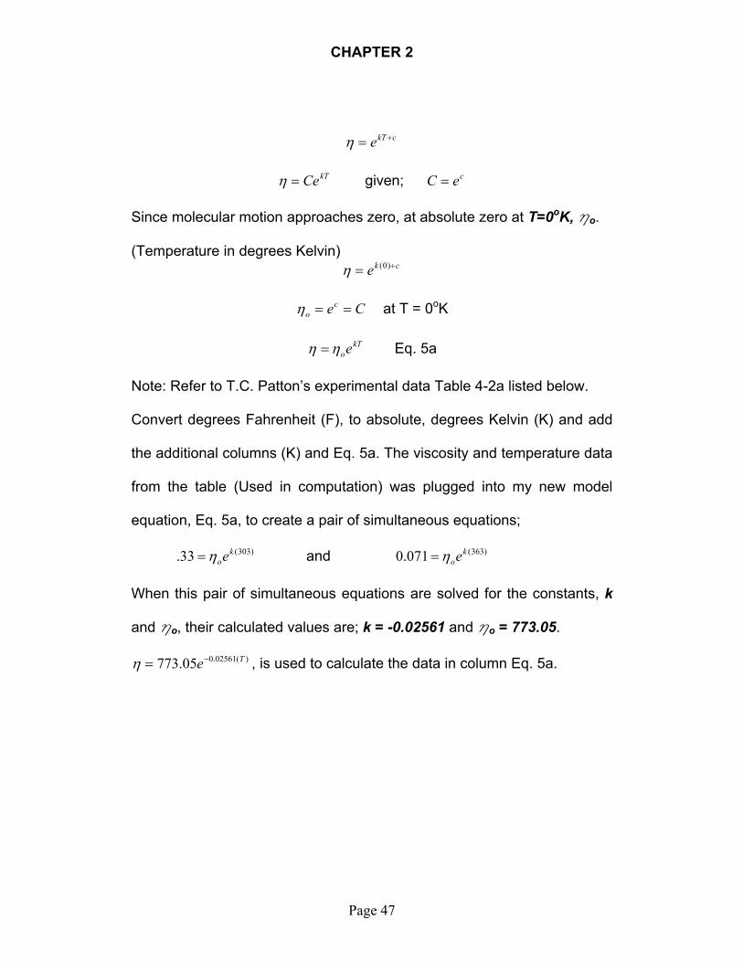
Since molecular motion approaches zero, at absolute zero at T=0oK, ho.
(Temperature in degrees Kelvin) cke += )0(η
Ceco ==η at T = 0oK
kToeηη = Eq. 5a
Note: Refer to T.C. Patton’s experimental data Table 4-2a listed below.
Convert degrees Fahrenheit (F), to absolute, degrees Kelvin (K) and add
the additional columns (K) and Eq. 5a. The viscosity and temperature data
from the table (Used in computation) was plugged into my new model
equation, Eq. 5a, to create a pair of simultaneous equations;
)303(33. koeη= and )363(071.0 k
oeη=
When this pair of simultaneous equations are solved for the constants, k
and ho, their calculated values are; k = -0.02561 and ho = 773.05.
)(02561.005.773 Te−=η , is used to calculate the data in column Eq. 5a.
Page 47
CHAPTER 2
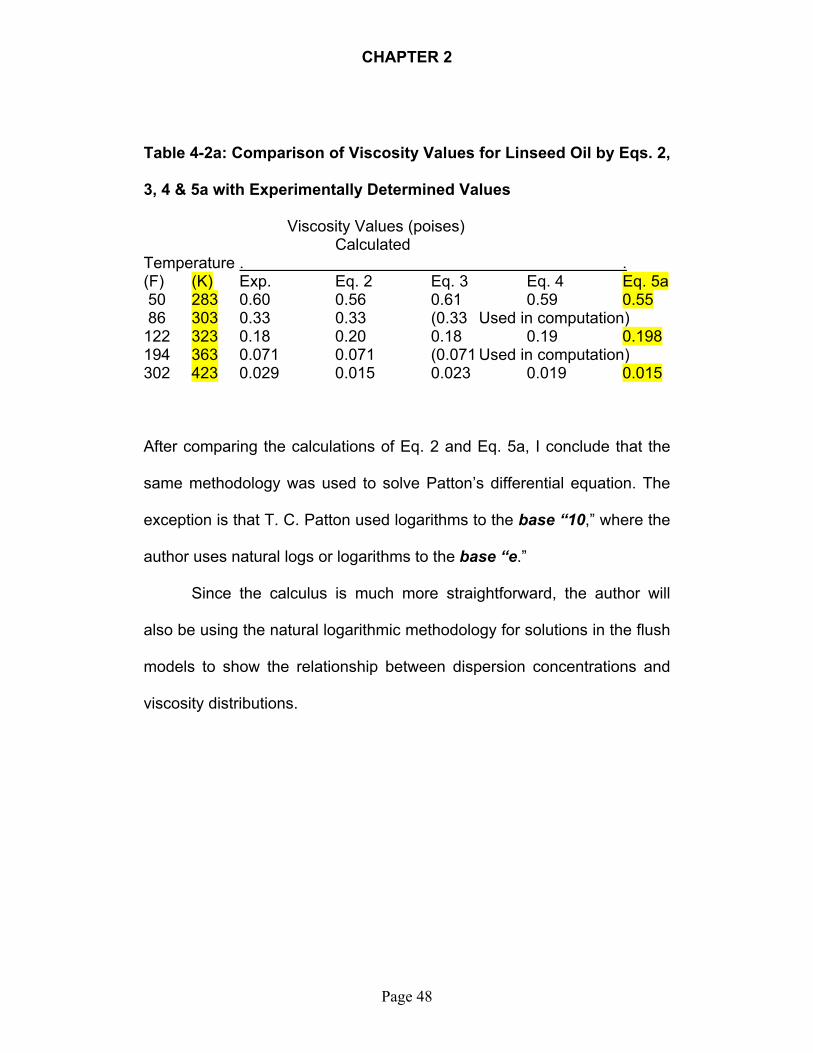
Table 4-2a: Comparison of Viscosity Values for Linseed Oil by Eqs. 2,
3, 4 & 5a with Experimentally Determined Values
Viscosity Values (poises) Calculated
Temperature . . (F) (K) Exp. Eq. 2 Eq. 3 Eq. 4 Eq. 5a 50 283 0.60 0.56 0.61 0.59 0.55 86 303 0.33 0.33 (0.33 Used in computation) 122 323 0.18 0.20 0.18 0.19 0.198 194 363 0.071 0.071 (0.071 Used in computation) 302 423 0.029 0.015 0.023 0.019 0.015
After comparing the calculations of Eq. 2 and Eq. 5a, I conclude that the
same methodology was used to solve Patton’s differential equation. The
exception is that T. C. Patton used logarithms to the base “10,” where the
author uses natural logs or logarithms to the base “e.”
Since the calculus is much more straightforward, the author will
also be using the natural logarithmic methodology for solutions in the flush
models to show the relationship between dispersion concentrations and
viscosity distributions.
Page 48
CHAPTER 2
Engineering Mathematics
Stroud, K.A., 5th edition (2001)
One of the models, Model-C, that will be created is based on the
geometric progression. The author found Stroud to be an excellent source
for reviewing the concepts relating to the Geometric Series. The
applications of geometric progression that first came to mind were
problems of finance, like compound interest.
Model-C uses sequences the pigment concentrations after each
break as a geometric series. If the pigment concentrations are geometric
in nature, then their pigment charges are geometric. A geometric model
will allow the progression elements to be summed by formula. The very
first illustration that Stroud uses in his chapter, Series 1, “Geometric series
(geometric progression), denoted by GP,” problem 11:
An example of a GP is the series:
1 + 3 + 9 + 27 + 81 + … etc.
Here you can see that any term can be written from the previous term
by multiplying it by a constant factor 3. This constant factor is called
the common ratio and is found by selecting any term and dividing it
by the previous one:
e.g. 27 39 =÷ ; 9 33 =÷ ; … etc.
Page 49

CHAPTER 2
A GP therefore has the form:
...32 ++++ ararara etc.
where, a = first term, r = common ratio.
(Stroud, 2001, p. 752)
When the author saw this example, he thought of the flush distribution of
pigment charges. The graph of the geometric sequence 1, 3 ,9, 27, 81, is
shown below.
0
10
20
30
40
50
60
70
80
90
1 2 3 4 5
Series1
To the author, it looks like the upside-down version of the exponential
graph in chapter 1. Therefore he felt that he should be able to manipulate
the sequence, mathematically and produce the exponential pattern. This is
what led to the creation of “Model-C, The Geometric Series.”
Page 50
CHAPTER 3
Page 51
METHODOLOGY
Approach
The initial idea which led to the development of this project was
conceived while serving in the capacity of a formulator whose duties were
to prepare the work orders and process the procedures in a pigment
manufacturing plant. The senior technologist was the person who initiated
the process by preparing the small research batches in the laboratory and
in the plant. Upon completion of the development stage, the plant
formulator would scale the procedure up so that it could be run in a
production size mixer.
After preparing numerous plant procedures for flush dispersions, a
common pattern was noticed about all of the procedures and that was the
pigment and vehicle charge distribution. As the mixing stages progressed
from the initial stage to the final stage, both the pigment and the vehicle
charges were always decreasing in amount. It was also noticed that the
viscosity of the dispersions seemed to be building in an exponential
growth curve pattern. It was also noticed that as the skeletal development
procedures were scaled up to production capacities, adjustments had to
be made because of a non-linear relationship between the material
distribution and the production mixer capacities.

CHAPTER 3
Page 52
Data Gathering Method
The need to make the connection between material distribution and
the mixer capacity sparked an interest and curiosity, which led to an in-
depth journey into the research of pigment and paint dispersions. The
subject matter was a scientific and mathematical excursion into the world
of measurement of viscosity and its applications.
Creating a mathematical model to simulate the flush procedure was
the best way try to produce the same patterns that kept showing up in the
plant work orders. The method by which the models were created can
best be described as mathematical. Most of the math focused on the
dynamics of growth functions and their applications. The viscosity
applications required the use of first order differential equations and the
algebra of exponential functions. The mixer capacity applications involved
summation algebra.
The methodology of the flush models had to be created with pure
mathematics and then modeled into programs. Once the models were
coded into program logic and math scripts, it was easier to experiment
with the parameters and their inter-relationship.
CHAPTER 3
Page 53
Database of Study
Most of the research literature was focused on dispersions and the
viscosity of resin solutions. Temple C. Patton’s “Paint Flow and Pigment
Dispersion” was the best resource for this project because of his
mathematical treatment of the subject.
Most of the math that was used in this project was a result of
cumulated mathematical training over the years. Some of the advanced
math required some review in the area of applied differential equations.
The mathematics of finance was a great resource for reviewing
applications of the infinite series.
MathCAD and Basic Programming were very useful tools in
creating and testing the models. They were very good resources for
producing quick results with minimum effort. My programming experience
came in very handy.
Validity of Data
The resource literature contained tables of experimental data that
served as a target for the models to reproduce. The primary strategy was
to use logical empirical modeling to reproduce the experimental results.
The validity of the output from the models will rely entirely on analysis. A
good model will closely mimic the experimental data.

CHAPTER 3
Page 54
Originality and Limitations of Data
There was very little literature found that would imply that this
approach to creating flush models has been attempted. The concept is
quite simple in nature, but because of the complexity of the technology
related to viscosity measurement and fluid dynamics, it gets quite involved
mathematically. The model output is empirical and it’s objective is to serve
as a tool for the ink technologist when analyzing flush procedures.
After the models were completed, they only opened the door to
more questions. These models only address the mixing stages as a
discrete function. There is so much more to be learned from the mixing
dynamics that take place between the stages. The focus of this project
limited and simplified the units of measure to obtain its objective.
However, there is much potential to advance this project and incorporate
the concepts of energy usage and manufacturing cost analysis.
Summary of Chapter 3
Most of the methods and techniques used in creating the models
for this project are simple and straightforward. The output of the models
can only be analyzed and compared to data that is documented within the
resource literature.

CHAPTER 3
Page 55
The core of the creation of the models lies within the chapters that
show the steps in the longhand mathematical development of the logical
functions and relationships from which the models are built. The proof
development will be shown in the appendix.

CHAPTER 4
Page 56
DATA ANALYSIS
Observed Process Reaction Per Mixing Stage (All Treatments)
A given amount of presscake, PW, is mixed with a given amount of vehicle,
V, to produce a paste, PV (wetted pigment) and displaced water, W.
Formula #23: PW V PV W
PW ……………………. Aqueous Pigment (Presscake)
W ……………………… Displaced Water
V ………………………. Resin or Resin Solution
PV = P+V ……………… Pigment wetting
P ……………………….. Pigment (Non Aqueous)
Given a mixer of bulk capacity (B), several mixing stages (i = 1, 2, 3, … n) of
aqueous pigment (PW) and vehicle (V) are charged to the mixer in calculated
amounts such that the charge (PW + V) in any given stage (i), plus the paste or
wetted pigment that has already been mixed in prior stages, will always equal or
be less than the bulk capacity (B).
Formula #24: Before Mixing
Bi
ii iP V PW V
1 2 3 11
, , ,...( )

CHAPTER 4
Page 57
Formula #25: After Mixing
WPVVP iii
iB
11,...3,2,1)(
The discharge of water, (Wi), after any stage of mixing creates the net capacity
for the next stage of additives, (Pi+1 + V i+1).
11 iii VPWW
221 iii VPWW
332 iii VPWW
…
WVPWW 1 given i1
Theoretically, this process could go on forever; i , but a point is rapidly
approached where a decision must be made to end the process. This final stage
is designated as the nth or last stage (n). So the final expression that shows Wn
is; nnnn WVPWW 1 given ni 1
The function or algorithm which approximates the number of stages required to
mix a total amount of pigment,
n
iiP
1
, having a solids contents of (r), with a total
amount of vehicle or resin solution,
n
iiV
1
, into a mixer vessel of bulk capacity (B),
is Formula #8;Bx
VPrn
np
n
i
n
ii
1 1
))(/1(. The ratio of total pigment charge

CHAPTER 4
Page 58
to total charge is designated as Formula #11, xpn.
n
iii
n
ii
pn
VP
Px
1
1
)(. This ratio
also is indirectly related to the number of stages (n) in Formula #8 above, which
is required to completely mix the pigment with the resin solution and displace all
of the water.
Treatment – I: MODEL (A) requires initial amounts of pigment and vehicle (non-
optimized) to be charged to the mixer. The model calculates the amounts of
pigment and vehicle charges that are required for each mixing stage so that the
sum of the increment charges will equal the optimized total charge. In other
words, this model distributes the total charge to agree with the given viscosity
distribution. Optimization is the primary focus of this treatment while adhering to
a given viscosity distribution and holding the mixer capacity constant. The
calculated capacity, B(i), is is an output parameter and will be listed at each
mixing stage to compare to the constant capacity, B. The input parameter, E0
(Allowance), is the estimated % of the constant capacity. Theoretically, E0 is
equal to the water displacement in the final mixing stage.
INPUT DATA OUTPUT DATA
Capacity Constant B Calculated Capacity at stage (i) B(i).
Initial Pigment Charge SP(i) Number of mixing stages (n)
Initial Vehicle ChargeSV(i) % Vehicle after last stage (xn)
Relative Viscosity of the Pigment (hp) System Viscosity Constant (kv)
Relative Viscosity of the Vehicle (hv) Viscosity Distribution h(i)

CHAPTER 4
Page 59
INPUT DATA (Continued) OUTPUT DATA (Continued)
% Solids of Presscake (r) % Pigment per stage xp(i)
Viscosity Distribution Function f(i) % Vehicle per stage xv(i)
Allowance E0 Pigment Charge per stage P(i)
Vehicle Charge per stage V(i)
Water Displacement per stage wd(i)
Total Pigment Charge SP(i)
Total Vehicle Charge SV(i)
Example Problem MODEL-A:
Given the non-optimized charge, SP(i) = 1350 lbs. SV(i) = 1200 lbs.
Relative Viscosity of the Pigment (hp) = 240,000 poise. Relative Viscosity of the
Vehicle (hv) = 100 poise. % Solids of Presscake (r) = 20%: (0.20). Capacity
Allowance E0 = 15%: (Eff% = 85% Refer to Formula #22). Optimize the flush
procedure to be mixed in a vessel of Capacity, B = 3000 lbs.
Solution Steps MODEL-A:
Step #1
Using Formula #11: Calculate the % pigment (xp)in total charge.
)58.120242.1347(42.1347
)(1
1))((%
1
n
iii
n
ii
BEff
P
p
VP
Px
n
ii
= 0.5294
1 pv xx ; pv xx 1 5294.01vx 4706.0vx
Step #2

CHAPTER 4
Page 60
Using Formula #8: Estimate the number of required mixing stages (n)
Formula #8 n = 4706.04706.0))(85.0()1( 20.0
)5294.00
n
p
v
vrx
xxE
= 5.7813
Round (5.7813) up to n = 6 Stage counter i, (1 to n); ni 1
Step #3
Using Formula #15 )ln(v
vk Viscosity Constant for the mix
7832.7)240000
100ln( vk
Step #4
Using Formula #16 vvxkpn e Viscosity of the mix
19.6159240000 )4706.0)(7832.7( en
Step #5
Using Formula #17)1ln(
n
a n Relative Viscosity Constant
1975.3165)16ln(
871.6110
a
Step #6
Using Formula #18 )]1[ln( iai Viscosity Distribution ni 1
Viscosity ( i) = (1) 2193.9477, (2) 3477.3249, (3) 4387.8955,
(4) 5094.1889, (5) 5671.2726, (6) 6159.1900

CHAPTER 4
Page 61
Step #7
Using Formula #26v
p
i
v kx
i
)ln(
% Vehicle Distribution given ( ni 1 )
ivx (1) 0.6032, (2) 0.5440, (3) 0.5142, (4) 0.4950, (5) 0.4812, (6) 0.4706
1 pv xx ; vp xx 1
ipx (1) 0.3968, (2) 0.4560, (3) 0.4858, (4) 0.5050, (5) 0.5188, (6) 0.5294
Step #8
Using Formula #19 Pi
Bx Pi
x
pii
i
r vi r
1
1
1 11( ) Pigment Distribution for ni 1
iP (1) 460.1058, (2) 321.4687, (3) 229.6540, (4) 166.8274,
(5) 123.0372, (6) 92.1022
n
iiP
11953.1393 Optimized
Step #9
Using Formula #6 ii
i PrPW Water displacement distribution ni 1
iW (1) 1840.4232, (2) 1285.8750, (3) 918.6159, (4) 667.3095,
(5) 492.1489, (6) 368.4088
Step #10
Using logic, 111 WPBV : 4232.18401058.46030001 V 4710.6991 V
rP
VBV 212 :
20.04687.321
4710.69930002 V 0795.2332 V
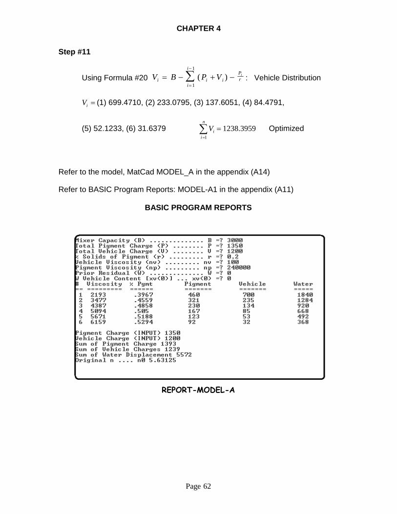
CHAPTER 4
Page 62
Step #11
Using Formula #20 V B P Vi i iPr
i
ii
( )1
1
: Vehicle Distribution
iV (1) 699.4710, (2) 233.0795, (3) 137.6051, (4) 84.4791,
(5) 52.1233, (6) 31.6379 3959.12381
n
iiV Optimized
Refer to the model, MatCad MODEL_A in the appendix (A14)
Refer to BASIC Program Reports: MODEL-A1 in the appendix (A11)
BASIC PROGRAM REPORTS
REPORT-MODEL-A

CHAPTER 4
Page 63
Treatment – II- MODEL-B requires (xp), the % pigment in the total mix, as an
input parameter. This parameter along with the capacity, B, is used to calculate
the initial pigment and vehicle charges, which are required as input parameters in
Treatment-I. The remaining steps of the procedure and the objectives are
identical to Treatment-I. The model uses the mixer’s capacity along with the
viscosity distribution as the critical input parameters to optimize the loading of
each mixing stage and optimize the yield. The total amount of pigment and
vehicle required to charge the mixer is an output parameter in this procedure.
INPUT DATA OUTPUT DATA
Mixer Capacity (B) Number of mixing stages (n)
% Pigment after last stage (xp) % Vehicle after last stage (xn)
Relative Viscosity of the Pigment ( p ) System Viscosity Constant (kv)
Relative Viscosity of the Vehicle ( v ) Viscosity Distribution )( i
% Solids of Presscake (r) % Pigment per stage xp(i)
Viscosity Distribution Function f(i) % Vehicle per stage xv(i)
Allowance E0 Pigment Charge per stage P(i)
Vehicle Charge per stage V(i)
Water Displacement per stage wd(i)
Total Pigment Charge SP(i))
Total Vehicle Charge SV(i)
Calculated Capacity at stage (i) B(i)

CHAPTER 4
Page 64
Example Problem MODEL-B:
Given the Pigment Content of the mix (xp)=0.5294, Relative Viscosity of
the Pigment (hp) = 240,000 poise. Relative Viscosity of the Vehicle (hv) = 100
poise. % Solids of Presscake (r) = 20%: (0.20). Capacity Allowance E0 = 15%:
(Eff% = 85% Refer to Formula #22). Optimize the flush procedure to be mixed in
a vessel of Capacity, B = 3000 lbs.
Note: Given the same input parameters of MODEL-A with the exception
being (xp), which is a calculated output parameter, the output of MODEL-B is
expected to be the same as the optimized output of MODEL-A.
Solution Steps MODEL-B:
Step #1
Calculate the % vehicle (xv)in the total charge.
1 pv xx ; pv xx 1 5294.01vx 4706.0vx
Step #2
Using Formula #8: Estimate the number of required mixing stages (n)
#8 n =4706.0
4706.0))(85.0()1( 20.0)5294.0
0
n
p
v
vrx
xxE
= 5.7813
Round (5.781) up to n = 6 Stage counter i, (1 to n); ni 1
Step #3
Using Formula #15 )ln(v
vk Viscosity Constant for the mix
7832.7)240000
100ln( vk
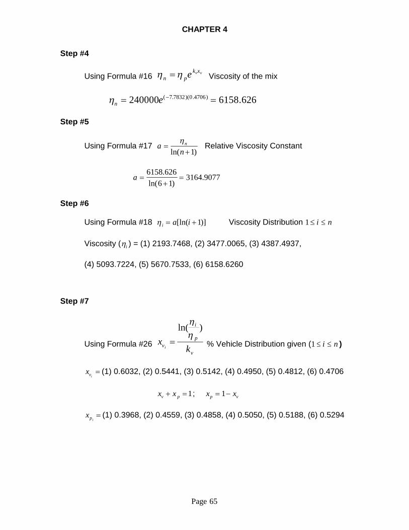
CHAPTER 4
Page 65
Step #4
Using Formula #16 vvxkpn e Viscosity of the mix
626.6158240000 )4706.0)(7832.7( en
Step #5
Using Formula #17)1ln(
n
a n Relative Viscosity Constant
9077.3164)16ln(
626.6158
a
Step #6
Using Formula #18 )]1[ln( iai Viscosity Distribution ni 1
Viscosity ( i) = (1) 2193.7468, (2) 3477.0065, (3) 4387.4937,
(4) 5093.7224, (5) 5670.7533, (6) 6158.6260
Step #7
Using Formula #26v
p
i
v kx
i
)ln(
% Vehicle Distribution given ( ni 1 )
ivx (1) 0.6032, (2) 0.5441, (3) 0.5142, (4) 0.4950, (5) 0.4812, (6) 0.4706
1 pv xx ; vp xx 1
ipx (1) 0.3968, (2) 0.4559, (3) 0.4858, (4) 0.5050, (5) 0.5188, (6) 0.5294
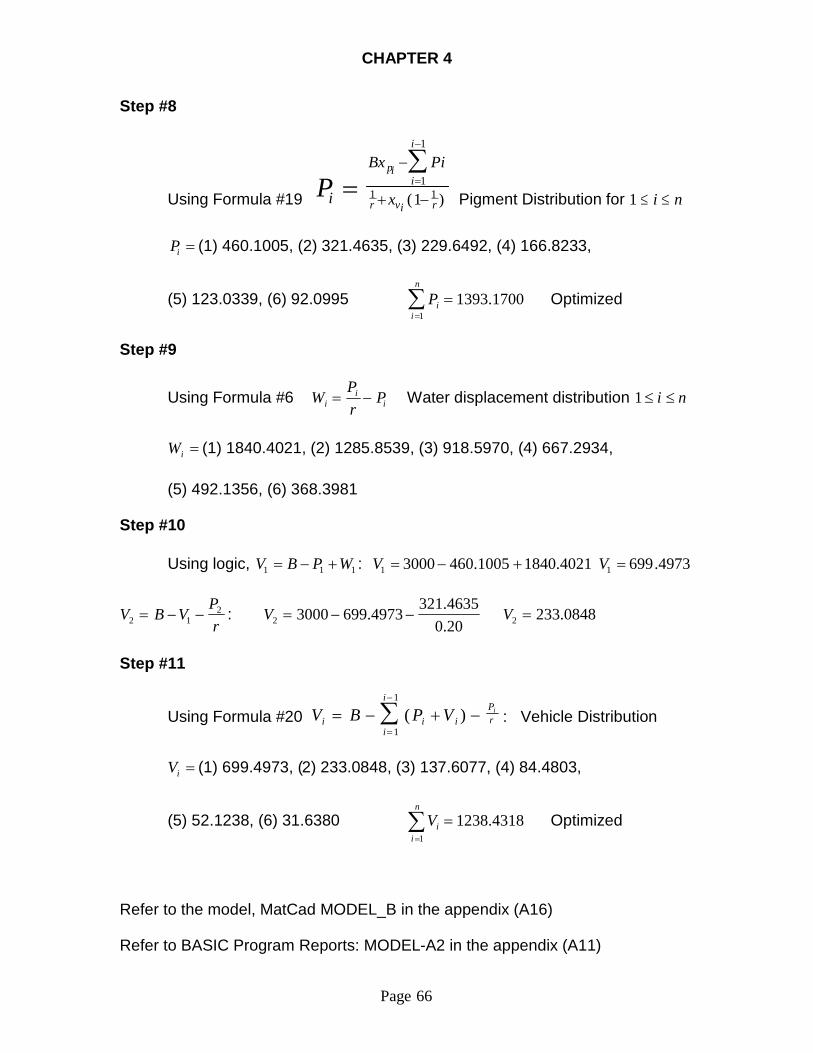
CHAPTER 4
Page 66
Step #8
Using Formula #19 Pi
Bx Pi
x
pii
i
r vi r
1
1
1 11( ) Pigment Distribution for ni 1
iP (1) 460.1005, (2) 321.4635, (3) 229.6492, (4) 166.8233,
(5) 123.0339, (6) 92.0995
n
iiP
11700.1393 Optimized
Step #9
Using Formula #6 ii
i PrP
W Water displacement distribution ni 1
iW (1) 1840.4021, (2) 1285.8539, (3) 918.5970, (4) 667.2934,
(5) 492.1356, (6) 368.3981
Step #10
Using logic, 111 WPBV : 4021.18401005.46030001 V 4973.6991 V
rP
VBV 212 :
20.04635.321
4973.69930002 V 0848.2332 V
Step #11
Using Formula #20 V B P Vi i iPr
i
ii
( )1
1
: Vehicle Distribution
iV (1) 699.4973, (2) 233.0848, (3) 137.6077, (4) 84.4803,
(5) 52.1238, (6) 31.6380 4318.12381
n
iiV Optimized
Refer to the model, MatCad MODEL_B in the appendix (A16)
Refer to BASIC Program Reports: MODEL-A2 in the appendix (A11)

CHAPTER 4
Page 67
BASIC PROGRAM REPORTS
REPORT-MODEL-B
Graph Actual Relative Viscosity vs Stage
Stage Viscosity1 21912 34733 43824 50875 56646 6151
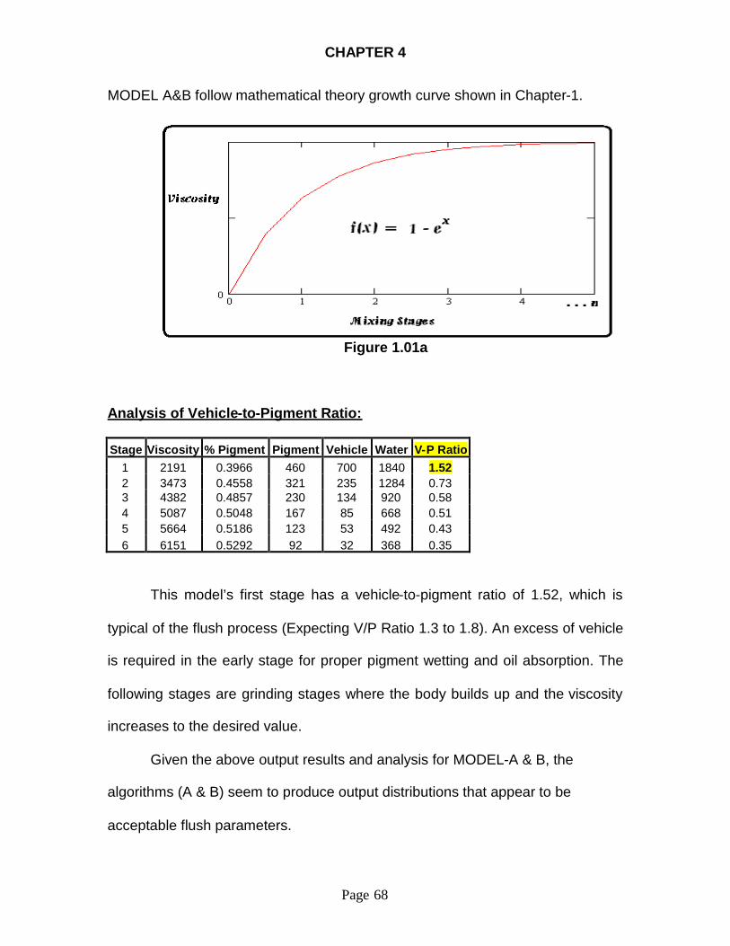
CHAPTER 4
Page 68
MODEL A&B follow mathematical theory growth curve shown in Chapter-1.
Figure 1.01a
Analysis of Vehicle-to-Pigment Ratio:
Stage Viscosity % Pigment Pigment Vehicle Water V-P Ratio1 2191 0.3966 460 700 1840 1.522 3473 0.4558 321 235 1284 0.733 4382 0.4857 230 134 920 0.584 5087 0.5048 167 85 668 0.515 5664 0.5186 123 53 492 0.436 6151 0.5292 92 32 368 0.35
This model’s first stage has a vehicle-to-pigment ratio of 1.52, which is
typical of the flush process (Expecting V/P Ratio 1.3 to 1.8). An excess of vehicle
is required in the early stage for proper pigment wetting and oil absorption. The
following stages are grinding stages where the body builds up and the viscosity
increases to the desired value.
Given the above output results and analysis for MODEL-A & B, the
algorithms (A & B) seem to produce output distributions that appear to be
acceptable flush parameters.

CHAPTER 4
Page 69
Treatment – III-MODEL-C uses the input parameter, Total Pigment Charge
SP(i), to create the pigment distribution, P(i). In this model, the pigment
distribution is a geometric progression, whose sum is equal to the input total
pigment charge, SP(i). The number of terms in the geometric progression, (n), is
treated as the number of mixing stages in the flush procedure. The viscosity
distribution is an output parameter based on the actual % pigment, xp(i),
calculated at each incremental stage (i). The mixer capacity, B, is held constant
through out the procedure. The calculated capacity B(i), is is an output parameter
and will be listed at each mixing stage to compare to the constant capacity, B. In
this treatment, the allowance, E0, is not required or used.
INPUT DATA OUTPUT DATA
Total Pigment Charge SP(i) Number of mixing stages (n)
Total Vehicle Charge SV(i) % Vehicle after last stage (xn)
Relative Viscosity of the Pigment (hp) System Viscosity Constant (kv)
Relative Viscosity of the Vehicle (hv) Viscosity Distribution h (i)
% Solids of Presscake (r) % Pigment per stage xp(i)
Pigment Distribution Function f(i) % Vehicle per stage xv(i)
In a Geometric Progression model, Pigment Charge per stage P(i)
Capacity B(i) is Constant for all Vehicle Charge per stage V(i)
stages. (1 < i < n) Water Displacement per stage wd(i)
Total Pigment Charge SP(i)
Total Vehicle Charge SV(i)

CHAPTER 4
Page 70
Example Problem MODEL-C1 (Non-Optimized):
Given the charge, SP(i) = 1350 lbs. SV(i) = 1200 lbs. Relative Viscosity of
the Pigment (hp) = 240,000 poise. Relative Viscosity of the Vehicle (hv) = 100
poise. % Solids of Presscake (r) = 20%: (0.20). Capacity Allowance E0 = 15%:
(Eff% = 85% Refer to Formula #22). Optimize the flush procedure to be mixed in
a vessel of Capacity, B = 3000 lbs.
Solution Steps MODEL-C1 (Non-Optimized):
Step #1
Using Formula #11: Calculate the % pigment (xp)in total charge.
)58.120242.1347(42.1347
)(1
1))((%
1
n
iii
n
ii
BEff
P
p
VP
Px
n
ii
= 0.5294
1 pv xx ; pv xx 1 5294.01vx 4706.0vx
Step #2
Using Formula #8: Estimate the number of required mixing stages (n)
Formula #8 n =4706.0
4706.0))(85.0()1( 20.0)5294.0
0
n
p
v
vrx
xxE
= 5.7813
Round (5.781) up to n = 6 Stage counter i, (1 to n); ni 1
Step #3
Using Formula #22Bw
E n0 ; BEwn 0 450nw
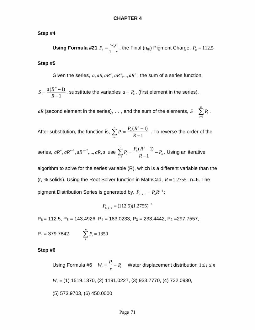
CHAPTER 4
Page 71
Step #4
Using Formula #21rrw
P nn
1, the Final (nth) Pigment Charge, 5.112nP
Step #5
Given the series, naRaRaRaRa ,...,,,, 32 , the sum of a series function,
1)1(
RRaS
n
, substitute the variables nPa , (first element in the series),
aR (second element in the series), … , and the sum of the elements,
n
iiPS
1.
After substitution, the function is,1
)1(1
RRP
Pn
nn
ii . To reverse the order of the
series, aaRaRaRaR nnn ,,...,,, 21 use n
nn
n
ii P
RRP
P
1
)1(1
. Using an iterative
algorithm to solve for the series variable (R), which is a different variable than the
(r, % solids). Using the Root Solver function in MathCad, 2755.1R ; n=6. The
pigment Distribution Series is generated by, 11
i
nin RPP :
116 )2755.1)(5.112( i
iP
P6 = 112.5, P5 = 143.4926, P4 = 183.0233, P3 = 233.4442, P2 =297.7557,
P1 = 379.7842 n
iiP 1350
Step #6
Using Formula #6 ii
i PrP
W Water displacement distribution ni 1
iW (1) 1519.1370, (2) 1191.0227, (3) 933.7770, (4) 732.0930,
(5) 573.9703, (6) 450.0000

CHAPTER 4
Page 72
Step #7
Using, 111 WPBV : 1370.15197842.37930001 V 0788.11011 V
Using,rP
VBV 212 :
20.07557.297
7842.37930002 V 3586.302 V
Using Formula #20
1
1)(
i
i
iiii r
PVPBV , given ni 1 ; generates
Vi = (1); 1101.0788, (2); 30.3586, (3); 23.8015, (4); 18.6607, (5); 14.6302,
(6); 11.4703 n
iiV 1200
Step #8
Using Formula #15 )ln(v
vk Viscosity Constant for the mix
7832.7)240000
100ln( vk
Step #9
Using Formula #16 vvxkpn e Viscosity of the mix
19.6159240000 )4706.0)(7832.7( en
Step #10
Using
i
iii
i
ii
p
VP
Px
i
1
1
)(,
ii pv xx 1 generates,
xpi = (1); 0.2585, (2); 0.3745, (3); 0.4409, (4); 0.4824, (5); 0.5101, (6); 0.5294
xvi = (1); 0.7435, (2); 0.6255, (3); 0.5591, (4); 0.5176, (5); 0.4899, (6); 0.4706
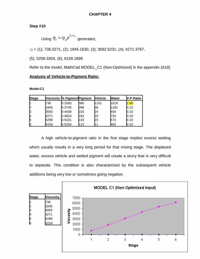
CHAPTER 4
Page 73
Step #10
Usingivvxk
pi e generates,
hi = (1); 736.0271, (2); 1845.1630, (3); 3092.5231, (4); 4271.3767,
(5); 5299.3304, (6); 6159.1899
Refer to the model, MathCad MODEL_C1 (Non-Optimized) in the appendix (A18)
Analysis of Vehicle-to-Pigment Ratio:
Model-C1
Stage Viscosity % PigmentPigment Vehicle Water V-P Ratio1 736 0.2565 380 1101 1519 2.902 1845 0.3745 298 30 1191 0.103 3093 0.4409 233 24 934 0.104 4271 0.4824 183 19 732 0.105 5299 0.5101 143 15 574 0.106 6159 0.5294 113 11 450 0.10
A high vehicle-to-pigment ratio in the first stage implies excess wetting
which usually results in a very long period for that mixing stage. The displaced
water, excess vehicle and wetted pigment will create a slurry that is very difficult
to separate. This condition is also characterized by the subsequent vehicle
additions being very low or sometimes going negative.
Stage Viscosity1 7362 18453 30934 42715 52996 6159

CHAPTER 4
Page 74
The graphic characteristic is a slow rise from the low viscosities to the end
mix viscosity. Too sharp of an increase implies a low vehicle-to-pigment ratio and
aggregation or large pigment clusters result. In summary, any drastic departure
from the exponential growth pattern below, is an indication of abnormality.
Figure 1.01a
Example Problem MODEL-C2 (Optimized):
Given the charge, SP(i) = 1393.1953 lbs. SV(i) = 1238.3959 lbs. Relative
Viscosity of the Pigment (hp) = 240,000 poise. Relative Viscosity of the Vehicle
(hv) = 100 poise. % Solids of Presscake (r) = 20%: (0.20). Capacity Allowance E0
= 15%: (Eff% = 85% Refer to Formula #22). Optimize the flush procedure to be
mixed in a vessel of Capacity, B = 3000 lbs.
Solution Steps MODEL-C2 (Optimized):

CHAPTER 4
Page 75
Step #1
Using Formula #11: Calculate the % pigment (xp)in total charge.
)58.120242.1347(42.1347
)(1
1))((%
1
n
iii
n
ii
BEff
P
p
VP
Px
n
ii
= 0.5294
1 pv xx ; pv xx 1 5294.01vx 4706.0vx
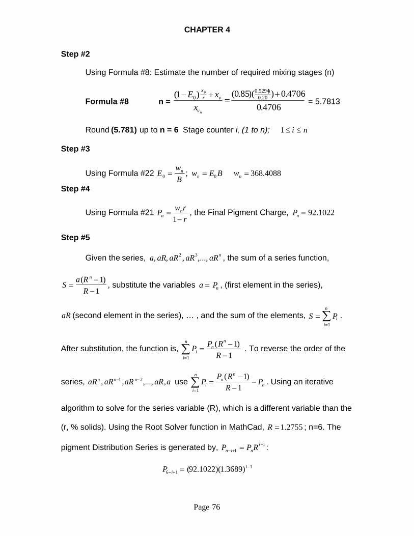
CHAPTER 4
Page 76
Step #2
Using Formula #8: Estimate the number of required mixing stages (n)
Formula #8 n =4706.0
4706.0))(85.0()1( 20.0)5294.0
0
n
p
v
vrx
xxE
= 5.7813
Round (5.781) up to n = 6 Stage counter i, (1 to n); ni 1
Step #3
Using Formula #22Bw
E n0 ; BEwn 0 4088.368nw
Step #4
Using Formula #21rrwP n
n
1, the Final Pigment Charge, 1022.92nP
Step #5
Given the series, naRaRaRaRa ,...,,,, 32 , the sum of a series function,
1)1(
RRa
Sn
, substitute the variables nPa , (first element in the series),
aR (second element in the series), … , and the sum of the elements,
n
iiPS
1
.
After substitution, the function is,1
)1(1
R
RPPn
nn
ii . To reverse the order of the
series, aaRaRaRaR nnn ,,...,,, 21 use n
nn
n
ii P
RRP
P
1
)1(1
. Using an iterative
algorithm to solve for the series variable (R), which is a different variable than the
(r, % solids). Using the Root Solver function in MathCad, 2755.1R ; n=6. The
pigment Distribution Series is generated by, 11
i
nin RPP :
116 )3689.1)(1022.92(
iiP

CHAPTER 4
Page 77
P6 = 92.1022, P5 = 126.0796, P4 = 172.5917, P3 = 236.2626, P2 =323.4222,
P1 = 442.7360 n
iiP 1943.1393
Step #6
Using Formula #6 ii
i PrPW Water displacement distribution ni 1
iW (1) 1770.9440, (2) 1293.6889, (3) 945.0502, (4) 690.3668,
(5) 504.3186, (6) 368.4088
Step #7
Using, 111 WPBV : 9440.17707360.44230001 V 3201.7861 V
Using,rP
VBV 212 :
20.04222.323736.44230002 V 8328.1532 V
Using Formula #20
1
1)(
i
i
iiii r
PVPBV , given ni 1 ; generates
Vi = (1); 786.3201, (2); 153.8328, (3); 112.3761, (4); 82.0917,
(5); 59.9686, (6); 43.8076 n
iiV 3969.1238
Step #8
Using Formula #15 )ln(v
vk Viscosity Constant for the mix
7832.7)240000
100ln( vk
Step #9
Using Formula #16 vvxkpn e Viscosity of the mix
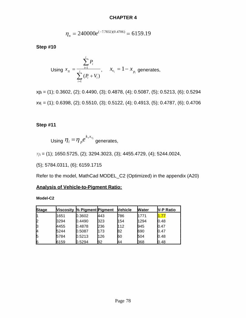
CHAPTER 4
Page 78
19.6159240000 )4706.0)(7832.7( en
Step #10
Using
i
iii
i
ii
p
VP
Px
i
1
1
)(,
ii pv xx 1 generates,
xpi = (1); 0.3602, (2); 0.4490, (3); 0.4878, (4); 0.5087, (5); 0.5213, (6); 0.5294
xvi = (1); 0.6398, (2); 0.5510, (3); 0.5122, (4); 0.4913, (5); 0.4787, (6); 0.4706
Step #11
Usingivvxk
pi e generates,
hi = (1); 1650.5725, (2); 3294.3023, (3); 4455.4729, (4); 5244.0024,
(5); 5784.0311, (6); 6159.1715
Refer to the model, MathCad MODEL_C2 (Optimized) in the appendix (A20)
Analysis of Vehicle-to-Pigment Ratio:
Model-C2
Stage Viscosity % Pigment Pigment Vehicle Water V-P Ratio1 1651 0.3602 443 786 1771 1.772 3294 0.4490 323 154 1294 0.483 4455 0.4878 236 112 945 0.474 5244 0.5087 173 82 690 0.475 5784 0.5213 126 60 504 0.486 6159 0.5294 92 44 368 0.48
CHAPTER 4
Page 79
This model’s first stage has a vehicle-to-pigment ratio of 1.77, which is
within the acceptable range (V/P Ratio 1.3 to 1.8). Comparing the ratio to
MODEL-A & MODEL-B, the expectation would be an adequate, but slightly
longer mixing period in the first wetting stage.
Given the above output results and analysis for MODEL-C2, the algorithm
(A & B) seems to produce the best output distributions if the pigment and vehicle
input charges are optimized.
CHAPTER 5
Page 80
SUMMARY, CONCLUSION AND RECCOMENDATIONS
Restatement of the Problem:
Quantifying the flush process is the primary focus of this project. By using
the general description of the flushing process, models can be created to
simulate the procedure. The three models, (MODEL-A, MODEL-B, MODEL-C),
uses bulk load capacity and viscosity as the major constraints to produce the
number of mixing stages and the component quantities that are required to
optimize the mixing process.
Since the vehicle-pigment ratio for each mixing stage is usually
determined by experimental methods in a laboratory environment, the main
objective in this project is to create some models and methodologies that
simulate this experimental process. If this objective is met, then this methodology
could possibly serve as a design and analysis tool which will increase the
productivity of the technologist.
SUMMARY
MODEL-A and MODEL-B
These two models are essentially the same in that they produce the same
output. The difference between the two models is that MODEL-B uses the end
mix pigment content and the mixer capacity to calculate the initial (non-
optimized) quantities. MODEL-B is more efficient in that it requires one less input
parameter while producing the same output. The end mix pigment content is also
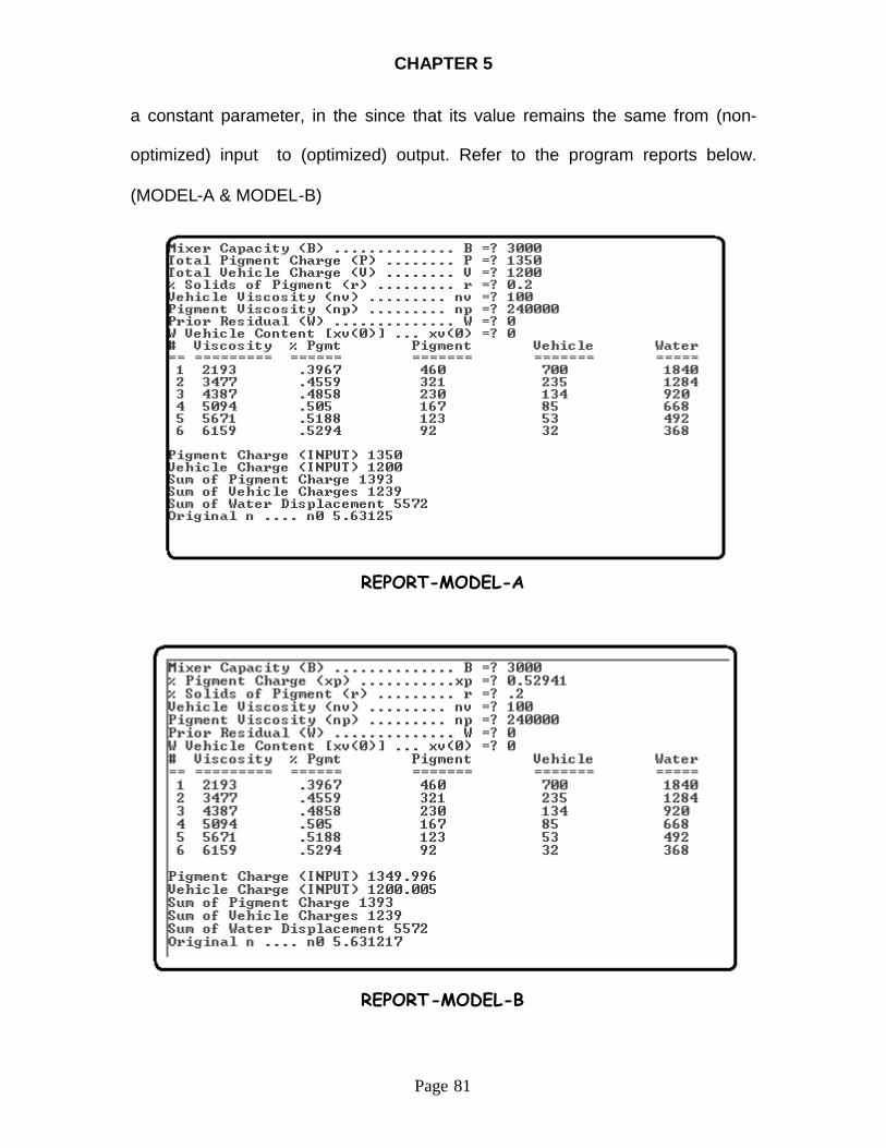
CHAPTER 5
Page 81
a constant parameter, in the since that its value remains the same from (non-
optimized) input to (optimized) output. Refer to the program reports below.
(MODEL-A & MODEL-B)
REPORT-MODEL-A
REPORT-MODEL-B

CHAPTER 5
Page 82
Using Formula #11: Calculate the % pigment (xp)in total charge in MODEL-A is:
)12001350(1350
)(1
1))((%
1
n
iii
n
ii
BEff
P
p
VP
Px
n
ii
= 0.52941,
which is the same as the INPUT % Pigment Charge xp in MODEL-B. Also note
the (non-optimized) INPUT Pigment Charge = 1349.996 & Vehicle Charge =
1200.005, are calculated by the program. Both program OUTPUT distributions
are very nearly identical.
The OUTPUT distributions of the two models resemble the beaker-spatula
mixing example shown below from Chapter-1 as Figure 1.02
Figure 1.02 (Flush Sequence)

CHAPTER 5
Page 83
MODEL-C1 & C2 (Geometric Series)
These two models, MODEL-C1 and MODEL-C2, use the geometric
function to determine the pigment content distribution, xp(i), instead of the
exponential growth function used in MODEL-A & B. The MODEL-C series does
not optimize the input charges, but creates the output distributions based on the
bulk capacity, B, and the allowance, E. The sum of the output charge distribution
is always equal to the total input charge.
VPINPUT ;: equals
n
i
n
iii VPOUTPUT
1 1;:
For comparative purposes, MODEL-C1 was created to use the (Non-
Optimized) pigment and vehicle charges that are inputs in MODEL-A & B, and
MODEL-C2 was created to use the (Optimized) charges that are outputs from
MODEL-A & B. Refer to the analysis of MODEL-C1 and MODEL-C2.
CONCLUSION
The output distributions generated form the flush models show that the
empirical derivations and implied relationships are accurate enough to serve as a
general outline for more complex models, which will provide further in-depth
analysis. I am certainly convinced that it is possible to model the flush procedure
with mathematical algorithms. There is much room for expansion of the models
to include more useful constraints such as temperature, time and energy
requirements. More detail design is needed prior to committing laboratory labor
CHAPTER 5
Page 84
and equipment to correlate and test the theoretical results to real dispersion
procedures.
As the project progressed into the analysis and summary phase, more
questions than answers were generated. I plan to continue working on this
project by fine-tuning the models and programs to be user-friendlier. There are
so many conditions, which need to be analyzed, but time and project format
constraints do not permit this at this time. I am very please with the development
of the mathematical logic and procedures, because the math is the foundation of
the modeling efforts.
RECOMENDATIONS
This phase of the project focused on the end result of the mixing (flushing)
stages and can best be characterized as empirical. The next phase of this project
is to do further analysis by testing more input conditions. There seems to be
some input values that will generate errors in the program during processing.
This needs to be investigated. The algorithm, which estimates the number of
required, mixing stages, needs more development.
Other conditions that were not addressed were the use of multiple input
vehicles and pigments of various viscosities. The use of solvents that evaporate
and agents that serve as catalysts, are also potential development
enhancements.

CHAPTER 5
Page 85
The related literature shows that temperature, shearing, pigment
absorption rates, evaporation rates, particle size and mixing speed are just some
of the many parameters that are directly related to the energy of mixing. The
action that occurs between the mixing stages is the most important part of the
flushing procedure and will require more detail treatment in the subsequent
phases. These and all of the items that were mentioned above are the
recommendations for future expansion and development. After all, the action that
occurs between the mixing stages is what is called “flushing.”

BIBLIOGRAPHY
Page 86
Atherton, D., Hedley, B, Greaves, J., Marks, S., Martin, S. & Smith, M.(1961). Paint Technology Manuals: PART TWO - Solvents, Oils, Resins and Driers: Published on behalf of The Oil & ColourChemists' Association
Atkins, P. W. (1982). Physical Chemistry. (2nd ed.). New York, SanFrancisco: W. H. Freeman and Company
Brothman, A, Wollan, G, & Feldman, S. (1947). Manual of ChemicalEngineering Calculations & Shortcuts: New Analysis ProvidesFormula to Solve Mixing Problems. New York: McGraw-HillPublishing Co., Inc.. Page 175
Giles, R. V. (June, 1962). Fluid Mechanics and Hydraulics: Schaum'sOutline Series. (2nd ed.). New York, St. Louis, San Francisco,Toronto, Sidney: McGraw-Hill Book Company
Kreyszig, E. (August 1988) Advanced Engineering Mathematics. (6th ed.).New York, Chichester, Brisbane, Toronto, Singapore: John Wiley &Sons
McKennell, R., Ferranti Ltd., Moston & Mancheser. (1960). A Reprint fromthe "Instrument Manual", 1960, Section XI: Ferranti InstrumentManual: The Measurement and Control of Viscosity And RelatedFlow Properties.
Patton, T. C. (1963). Paint Flow and Pigment Dispersion. (1st ed.). NewYork, Chichester, Brisbane, Toronto: John Wiley & Sons.
Patton, T. C. (1979). Paint Flow and Pigment Dispersion. (2nd ed.). NewYork, Chichester, Brisbane, Toronto: John Wiley & Sons.
Stroud, K.A., (2001). Engineering Mathematics. (5th ed.). New York:Industrial Press, Inc.
Turner, G. P. A (1967). Introduction to Paint Chemistry. London: Chapmanand Hall
Wolfe, H. J. (1967). Printing and Litho Inks. New York City: MacNair-Dorland Company

APPENDIX
A 1
FLUSH MODEL FORMULAE #1 r ( )0 1< <r :constant Solids content of aqueous pigment
#2 r P
P Wi
i ii
n
+=∑
1 Calculation of solids content
#3 i ( )0 ≤ ≤i n :integer Incremental flush stages #4 P Pi Pigment charge at stage, (i)
#5 V Vi Vehicle charge at stage, (i)
#6 W Wi Water displacement at stage, (i)
#7 W B P Vn ii
n
ii
n
= − += =∑ ∑( )
1 1 Water displacement at last stage, (n)
#8 n = ( / )( )1
11r P V
x B
ii
n
i
n
pn
+==∑∑
Calculation of the number of stages
required to flush the total charge of pigment and vehicle
#9 )(1
VP i
n
ii +∑
=
Total charge after water displacement
#10 B = Eff
VPn
iii
%
)(1∑
=
+ Bulk capacity or working mixer capacity
at % Effective (~ 85%; Decimal)
#11 xp
P
Eff B
ii
n
= =∑
1(% )( ) % pigment in total charge

APPENDIX
A 2
FLUSH MODEL FORMULAE
#12 x xp v= −1 % pigment in total charge
#13 xv
V
Eff Bi
i
n
= =∑
1(% )( ) % vehicle in total charge
#14 x xv p= −1
#15 kvv
p= ln( )η
η Viscosity constant in the Exponential
Viscosity Distribution
#16 η ηn pk xe v v= Relative End-Viscosity of the mix at stage (n)
#17 a nn= +η
ln( )1 Relative Viscosity Distribution Constant
#18 ηi a i= +ln( )1 Viscosity Distribution Function 1≤ ≤i n
#19 Pi
Bx Pi
x
pii
i
r vi r=
∑−
+ −=
−
1
1
1 11( ) Pigment Charge Distribution given 1≤ ≤i n

APPENDIX
A 3
FLUSH MODEL FORMULAE
#20 V B P Vi i i
Pr
i
ii= − + −
=
−
∑( )1
1
Vehicle Charge Distribution given 1≤ ≤i n
#21 Pw r
rnn=
−1 Final (nth) Pigment Charge given Pr n nn P w= +
#22 E wB
n0 = Allowance = (100 - % Effective)
#23 PW V PV W+ → + Physical reaction of presscake (PW),
mixing with vehicle, (V), to produce a paste of wetted pigment, (PV), and displaced water, (W).
#24 ∑−
=
+++≥1
1)(
i
iiii VPWVPB Expression of capacity (B), before
mixing and water displacement.
#25 ∑−
=
+++≥1
1)(
i
iiii WPVVPB Expression of capacity (B), after
mixing and water displacement.

APPENDIX
A 4
BASIC PROGRAMS MODEL-A
REM Pigment Distribution Bsaed On Viscosity Function Algorithm REM Created by Herb Norman Sr. for Mixer Problem Project (MODEL-A) REM 03/02/2005 - MODEL_A.BAS REM******************************************************* CLS REM Input Parameters REM ================= INPUT "Mixer Capacity (B) .............. B ="; B INPUT "Total Pigment Charge (P) ........ P ="; P INPUT "Total Vehicle Charge (V) ........ V ="; V INPUT "% Solids of Pigment (r) ......... r ="; r INPUT "Vehicle Viscosity (nv) ......... nv ="; nv INPUT "Pigment Viscosity (np) ......... np ="; np INPUT "Prior Residual (W) .............. W ="; W INPUT "W Vehicle Content [xv(0)] ... xv(0) ="; xv(0) REM B = 3000 REM P = 1350 REM V = 1200 REM r = .2 REM nv = 100 REM np = 240000 REM W = 0: xv(0) = 0 REM xv(0) = 0 REM Calculate Constants REM =================== P(0) = W * (1 - xv(0)) V(0) = W * xv(0) kv = LOG(nv / np) xv = V / (P + V): xp = (1 - xv) nmix = np * EXP(kv * xv) n = INT((P / r + V) / (xv * B) + .5) n0 = (P / r + V) / (xv * B) a = nmix / (LOG(n + 1)) REM Calculate Viscosity Distribution n(j)
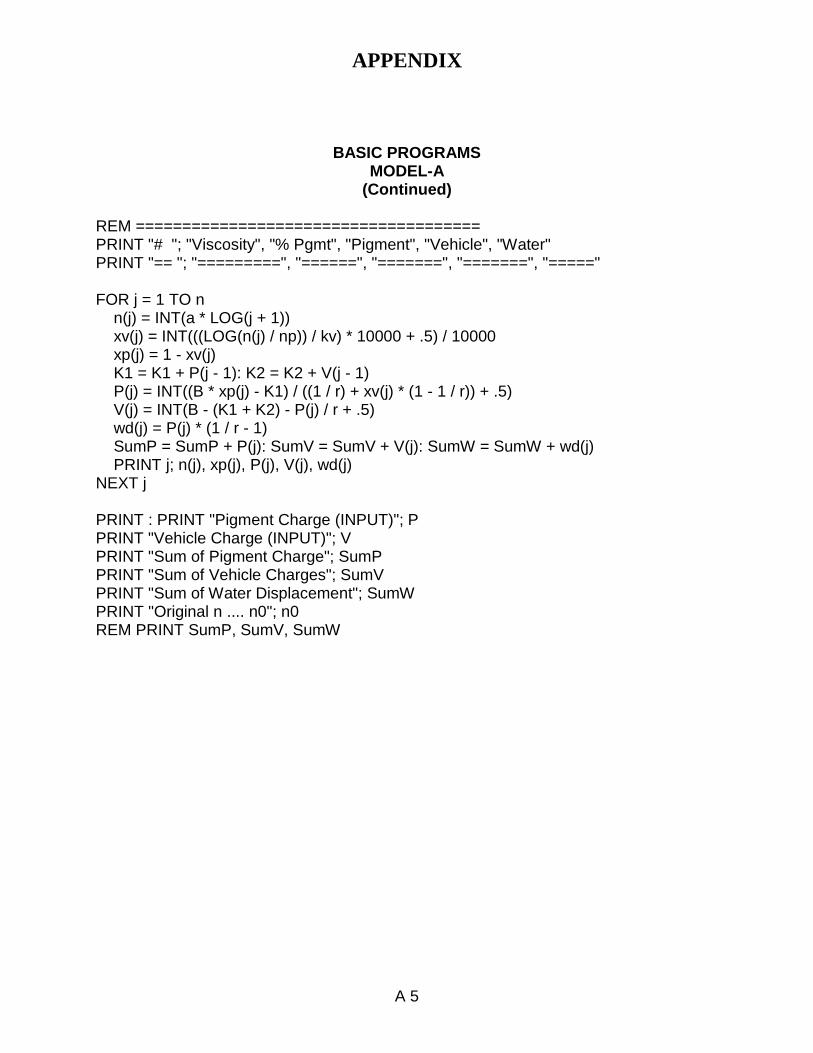
APPENDIX
A 5
BASIC PROGRAMS MODEL-A
(Continued) REM ===================================== PRINT "# "; "Viscosity", "% Pgmt", "Pigment", "Vehicle", "Water" PRINT "== "; "=========", "======", "=======", "=======", "=====" FOR j = 1 TO n n(j) = INT(a * LOG(j + 1)) xv(j) = INT(((LOG(n(j) / np)) / kv) * 10000 + .5) / 10000 xp(j) = 1 - xv(j) K1 = K1 + P(j - 1): K2 = K2 + V(j - 1) P(j) = INT((B * xp(j) - K1) / ((1 / r) + xv(j) * (1 - 1 / r)) + .5) V(j) = INT(B - (K1 + K2) - P(j) / r + .5) wd(j) = P(j) * (1 / r - 1) SumP = SumP + P(j): SumV = SumV + V(j): SumW = SumW + wd(j) PRINT j; n(j), xp(j), P(j), V(j), wd(j) NEXT j PRINT : PRINT "Pigment Charge (INPUT)"; P PRINT "Vehicle Charge (INPUT)"; V PRINT "Sum of Pigment Charge"; SumP PRINT "Sum of Vehicle Charges"; SumV PRINT "Sum of Water Displacement"; SumW PRINT "Original n .... n0"; n0 REM PRINT SumP, SumV, SumW
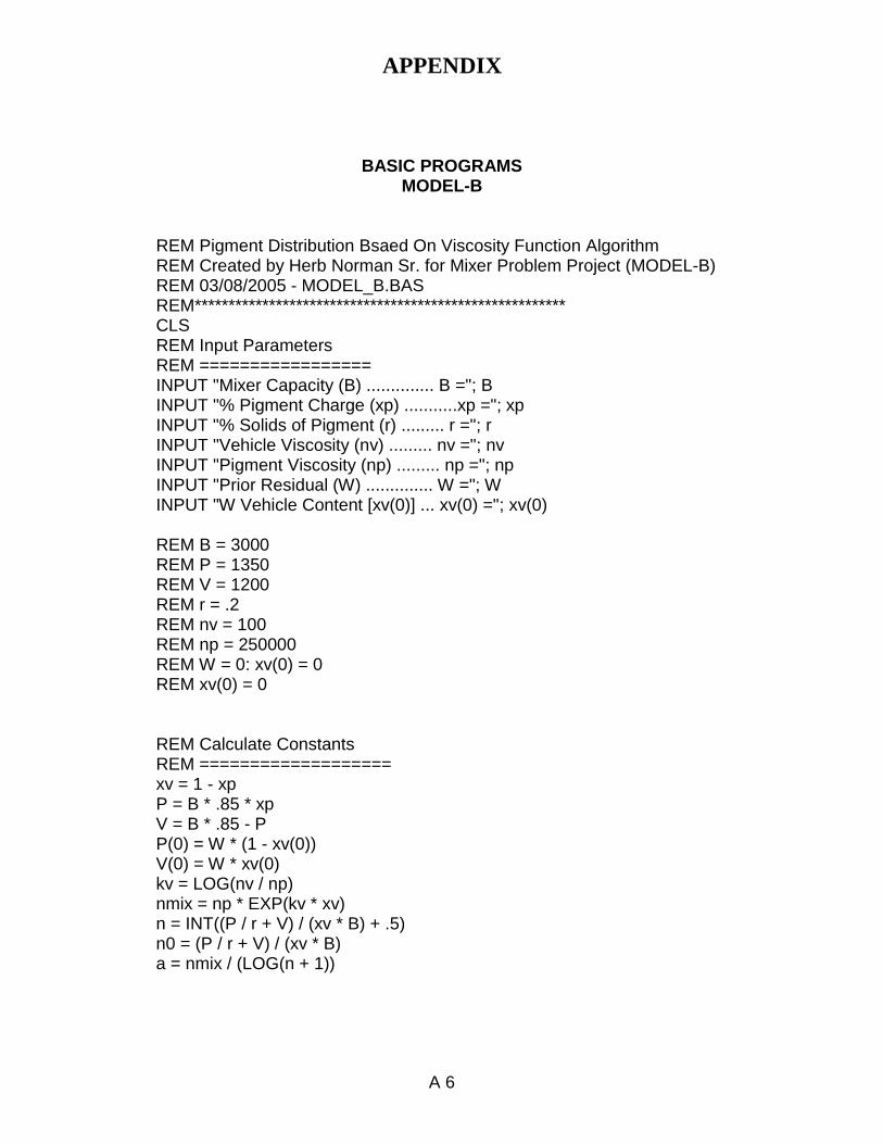
APPENDIX
A 6
BASIC PROGRAMS MODEL-B
REM Pigment Distribution Bsaed On Viscosity Function Algorithm REM Created by Herb Norman Sr. for Mixer Problem Project (MODEL-B) REM 03/08/2005 - MODEL_B.BAS REM******************************************************* CLS REM Input Parameters REM ================= INPUT "Mixer Capacity (B) .............. B ="; B INPUT "% Pigment Charge (xp) ...........xp ="; xp INPUT "% Solids of Pigment (r) ......... r ="; r INPUT "Vehicle Viscosity (nv) ......... nv ="; nv INPUT "Pigment Viscosity (np) ......... np ="; np INPUT "Prior Residual (W) .............. W ="; W INPUT "W Vehicle Content [xv(0)] ... xv(0) ="; xv(0) REM B = 3000 REM P = 1350 REM V = 1200 REM r = .2 REM nv = 100 REM np = 250000 REM W = 0: xv(0) = 0 REM xv(0) = 0 REM Calculate Constants REM =================== xv = 1 - xp P = B * .85 * xp V = B * .85 - P P(0) = W * (1 - xv(0)) V(0) = W * xv(0) kv = LOG(nv / np) nmix = np * EXP(kv * xv) n = INT((P / r + V) / (xv * B) + .5) n0 = (P / r + V) / (xv * B) a = nmix / (LOG(n + 1))

APPENDIX
A 7
BASIC PROGRAMS MODEL-B
(Continued) REM Calculate Viscosity Distribution n(j) REM ===================================== PRINT "# "; "Viscosity", "% Pgmt", "Pigment", "Vehicle", "Water" PRINT "== "; "=========", "======", "=======", "=======", "=====" FOR j = 1 TO n n(j) = INT(a * LOG(j + 1)) xv(j) = INT(((LOG(n(j) / np)) / kv) * 10000 + .5) / 10000 xp(j) = 1 - xv(j) K1 = K1 + P(j - 1): K2 = K2 + V(j - 1) P(j) = INT((B * xp(j) - K1) / ((1 / r) + xv(j) * (1 - 1 / r)) + .5) V(j) = INT(B - (K1 + K2) - P(j) / r + .5) wd(j) = P(j) * (1 / r - 1) SumP = SumP + P(j): SumV = SumV + V(j): SumW = SumW + wd(j) PRINT j; n(j), xp(j), P(j), V(j), wd(j) NEXT j PRINT : PRINT "Pigment Charge (INPUT)"; P PRINT "Vehicle Charge (INPUT)"; V PRINT "Sum of Pigment Charge"; SumP PRINT "Sum of Vehicle Charges"; SumV PRINT "Sum of Water Displacement"; SumW PRINT "Original n .... n0"; n0 REM PRINT SumP, SumV, SumW

APPENDIX
A 8
BASIC PROGRAMS MODEL-C
REM Iteration to find Ri factor in the Geometric Series REM Calculate Compoment Distribution & Relavive Viscosity Distribution REM Created by Herb Norman Sr. for Mixer Problem Thesis REM QBASIC PROGRAM - 03/15/2005 REM 1st Draft Thesis - 07/04/2005 REM Mathematical Model For A Mixing Optimizing Algorithm REM With Aqueous Displacement And Extraction REM Using Relative Viscosity And Mixer Capacity REM As the Primary Physical Constraints REM - An Application Of Geometric Series Distributions REM************************************************************************ CLS INPUT "Mixer Capacity (B) .............. B ="; B INPUT "Total Pigment Charge (P) ........ P ="; P INPUT "Total Vehicle Charge (V) ........ V ="; V INPUT "% Solids of Pigment (r) ......... r ="; r INPUT "Vehicle Viscosity (nv) ......... nv ="; nv INPUT "Pigment Viscosity (np) ......... np ="; np e = 2.7183 ex = .5 np = 240000! nv = 100 kv = LOG(nv / np) xp = P / (P + V) n = INT(((P / r + V) / (xp * B)) + .5) pn = (r / (1 - r)) * (B - (P + V)) REM *** Start Iteration - Solve for (Ri) & Final Pigment Charge P(n) FOR x = 1 TO 1000 Ri = 1 + (x / 1000) y = (pn * ((Ri ^ n) - 1)) / (Ri - 1) IF y >= (P - ex) THEN IF y <= (P + ex) THEN Rx = Ri END IF END IF NEXT x
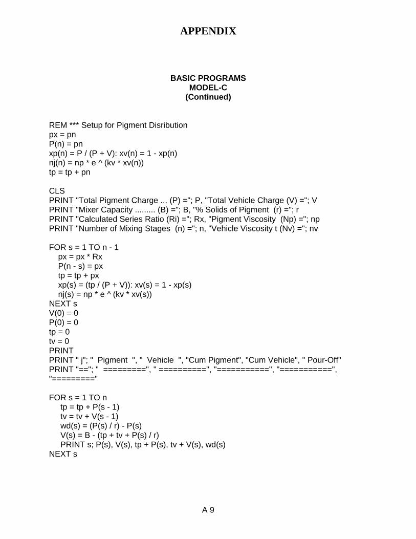
APPENDIX
A 9
BASIC PROGRAMS MODEL-C
(Continued) REM *** Setup for Pigment Disribution px = pn P(n) = pn xp(n) = P / (P + V): xv(n) = 1 - xp(n) nj(n) = np * e ^ (kv * xv(n)) tp = tp + pn CLS PRINT "Total Pigment Charge ... (P) ="; P, "Total Vehicle Charge (V) ="; V PRINT "Mixer Capacity ......... (B) ="; B, "% Solids of Pigment (r) ="; r PRINT "Calculated Series Ratio (Ri) ="; Rx, "Pigment Viscosity (Np) ="; np PRINT "Number of Mixing Stages (n) ="; n, "Vehicle Viscosity t (Nv) ="; nv FOR s = 1 TO n - 1 px = px * Rx P(n - s) = px tp = tp + px xp(s) = (tp / (P + V)): xv(s) = 1 - xp(s) nj(s) = np * e ^ (kv * xv(s)) NEXT s V(0) = 0 P(0) = 0 tp = 0 tv = 0 PRINT PRINT " j"; " Pigment ", " Vehicle ", "Cum Pigment", "Cum Vehicle", " Pour-Off" PRINT "=="; " =========", " ==========", "===========", "===========", "=========" FOR s = 1 TO n tp = tp + P(s - 1) tv = tv + V(s - 1) wd(s) = (P(s) / r) - P(s) V(s) = B - (tp + tv + P(s) / r) PRINT s; P(s), V(s), tp + P(s), tv + V(s), wd(s) NEXT s
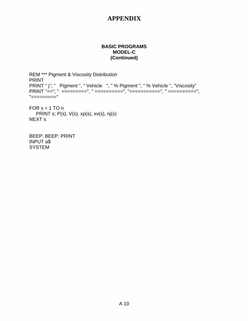
APPENDIX
A 10
BASIC PROGRAMS MODEL-C
(Continued) REM *** Pigment & Viscosity Distribution PRINT PRINT " j"; " Pigment ", " Vehicle ", " % Pigment ", " % Vehicle ", "Viscosity" PRINT "=="; " =========", " ==========", "===========", " ==========", "=========" FOR s = 1 TO n PRINT s; P(s), V(s), xp(s), xv(s), nj(s) NEXT s BEEP: BEEP: PRINT INPUT a$ SYSTEM

APPENDIX
A 11
BASIC PROGRAM REPORTS
REPORT-MODEL-A1
REPORT MODEL-A2

APPENDIX
A 12
BASIC PROGRAM REPORTS
REPORT MODEL-B1
REPORT MODEL-B2
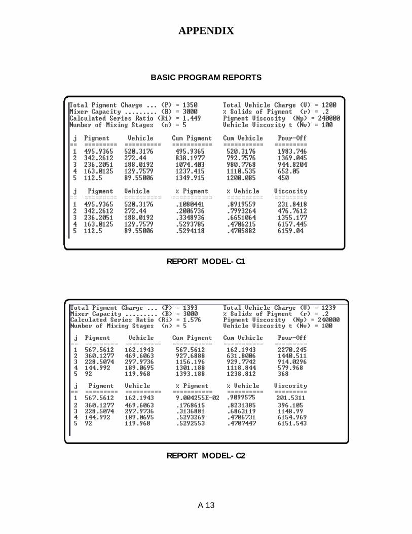
APPENDIX
A 13
BASIC PROGRAM REPORTS
REPORT MODEL-C1
REPORT MODEL-C2

A 14
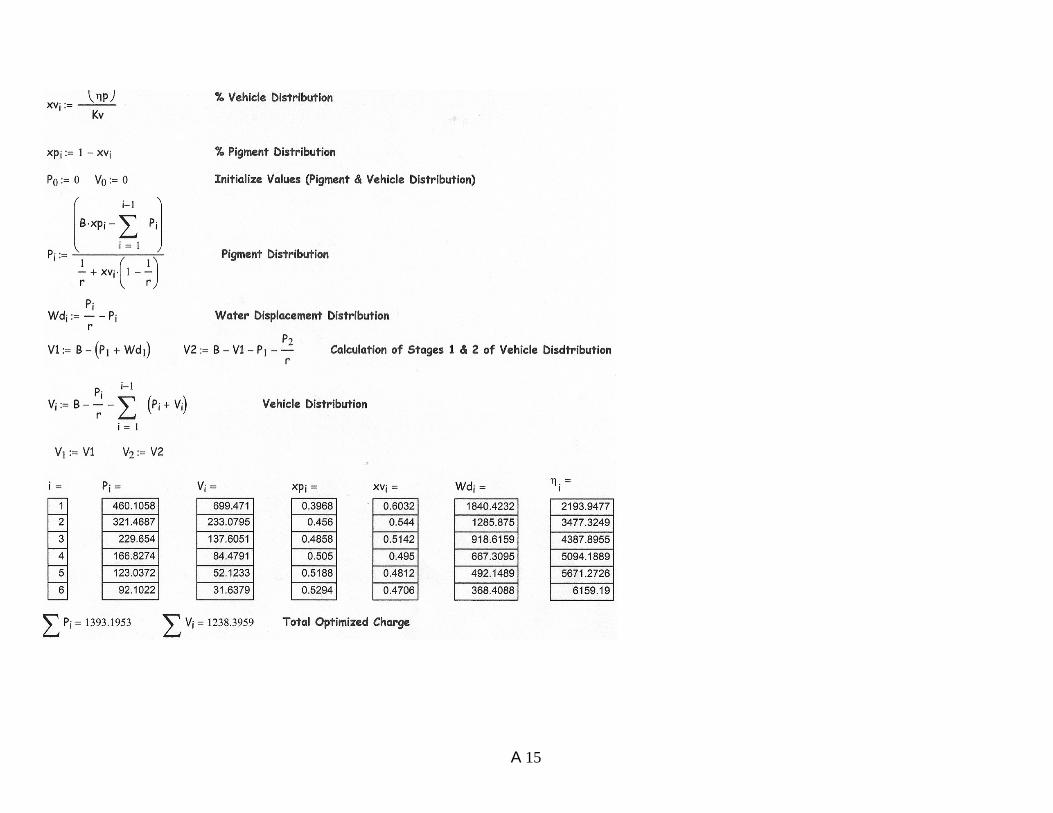
A 15

A 16
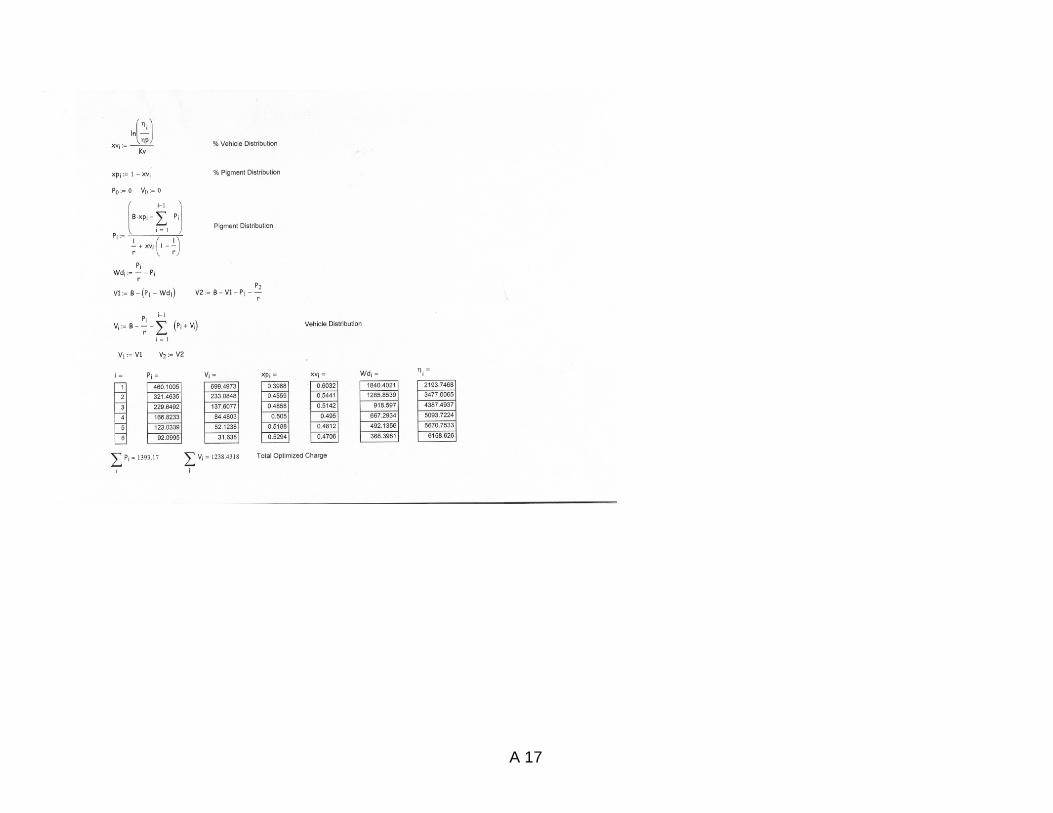
A 17

A 18

A 19
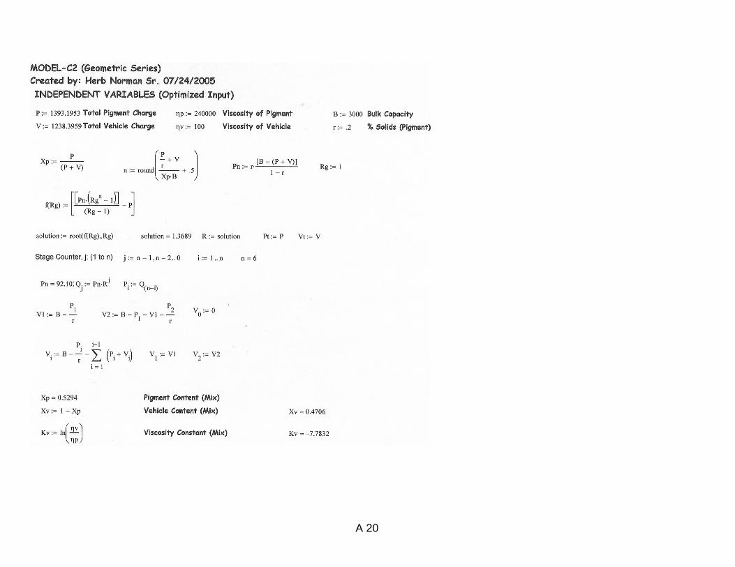
A 20
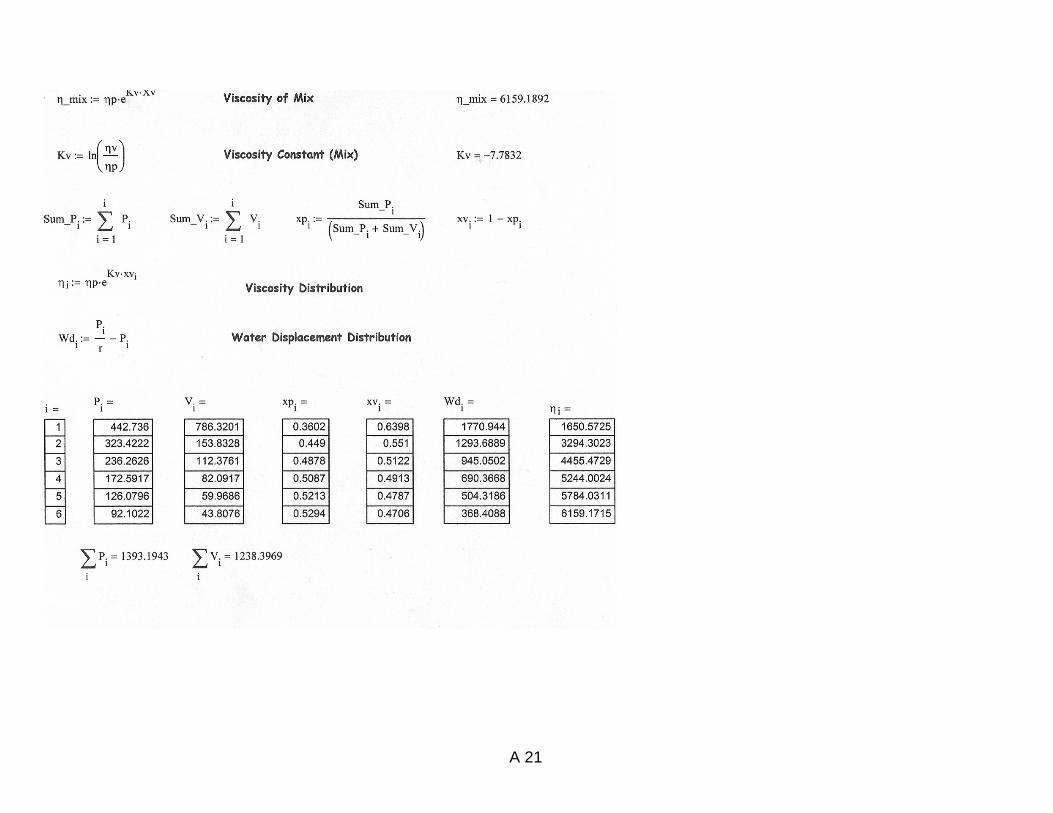
A 21

APPENDIX – B
B 1
FLUSH FORMULA DERIVATIONS
Solids Content of Pigment Presscake (r)Formula #2
Given the total pigment charge,
n
iiP
1
, the presscake is;
n
ii
n
ii
n
ii
WPr
P
11
1
rWP
P
i
n
ii
n
ii
)(1
1
Water Displacement at stage (i)Formula #6
Given the charge of presscake at stage (i),rPi
iii PW
rP
iii WP
rP
ii Wr
P )11
(

APPENDIX – B
B 2
Water Displacement (W) at stage (n)Formula #7
Given the capacity, B:
1
1
)(n
innnii VWPVPB
n
inii WVPB
1)(
)(11
n
ii
n
iin VPBW
Bulk Capacity, Allowance & % Effective (B), (E0) & (%Eff)Formula #10
Given capacity,
n
inii WVPB
1)( and )1% EoEff
0
11
1
)(
%
)(
E
VP
Eff
VPB
n
iii
n
iii
)()(%1
i
n
ii VPBEff
01 1
)(% E
B
VPEff
n
iii
BEBEffVPn
iii )1()(%)( 0
1
% Pigment in Total Charge xpFormula #11
Given Total Charge,
n
i
n
iii
n
iii VPVP
1 11)(
)(%)(
1
1
1
BEff
P
VP
Px
n
ii
n
iii
n
ii
p
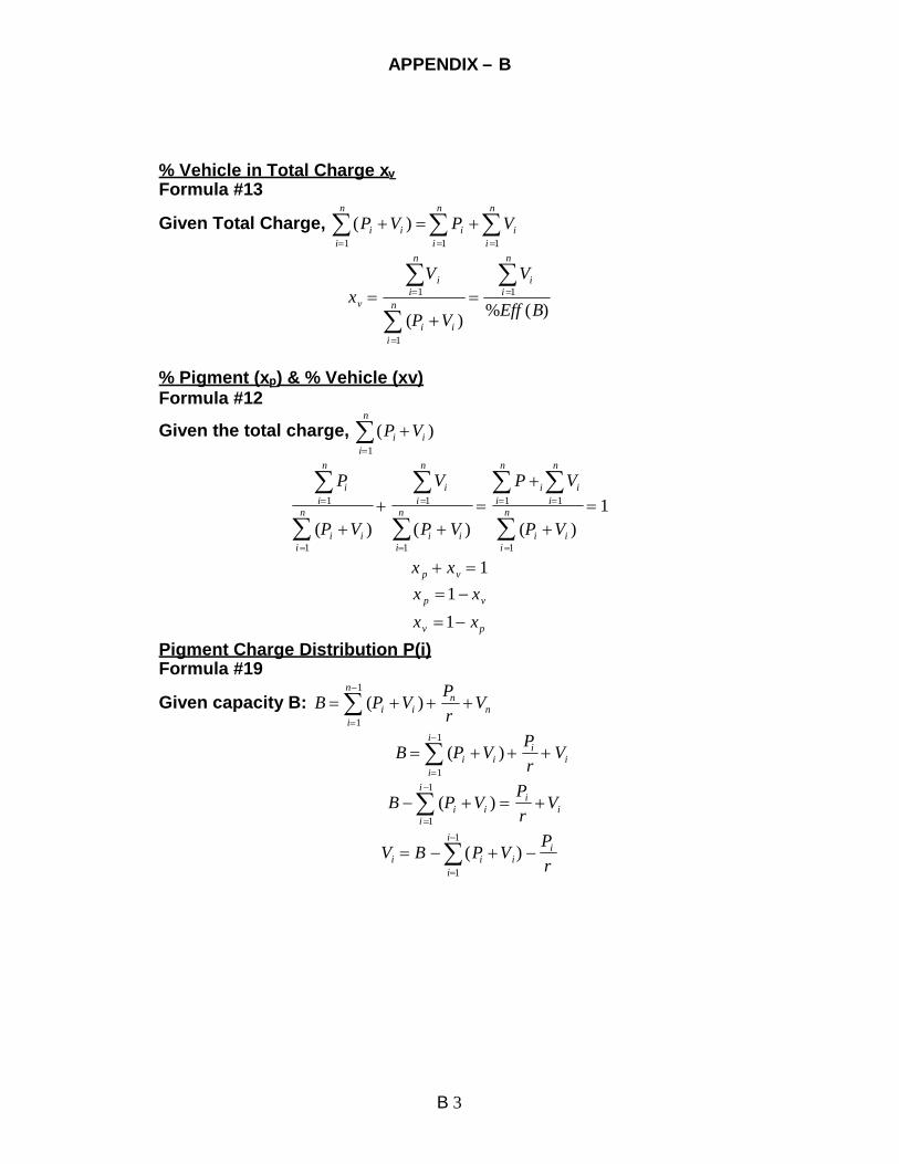
APPENDIX – B
B 3
% Vehicle in Total Charge xvFormula #13
Given Total Charge,
n
i
n
iii
n
iii VPVP
1 11
)(
)(%)(
1
1
1
BEff
V
VP
Vx
n
ii
n
iii
n
ii
v
% Pigment (xp) & % Vehicle (xv)Formula #12
Given the total charge,
n
iii VP
1
)(
1)()()(
1
11
1
1
1
1
n
iii
n
ii
n
ii
n
iii
n
ii
n
iii
n
ii
VP
VP
VP
V
VP
P
1 vp xx
vp xx 1
pv xx 1Pigment Charge Distribution P(i)Formula #19
Given capacity B:
1
1
)(n
in
nii V
rP
VPB
1
1
)(i
ii
iii V
rP
VPB
1
1)(
i
ii
iii V
rP
VPB
1
1
)(i
i
iiii r
PVPBV

APPENDIX – B
B 4
Pigment Charge Distribution P(i) (Continued)
n
iii
j
iji
j
VP
VVxv
v
1
1
1
)(
1
11
)(j
iji
j
iiij VVVPxv
1
11
)(j
iji
j
iiij VVVPxv
Equation Set:
1
1)(
i
i
iiii r
PVPBV
1
111
)(j
i
j
iiijj VVPxvV
jj VV
1
1
1
1
1
1
1
1)()()(
j
ii
j
i
j
i
jiijiij
j
i
jii V
rP
VPBPVPxvrP
VPB
1
1
1
1)(
j
ii
jjj
j
i
jii VB
rP
PxvrP
VPB
1
1
1
1
1
1
j
ii
jjj
j
i
jj
iii VB
rP
PxvrP
VPB
Br
PxvVrP
VPB jj
j
ii
j
i
jj
iii )
11(
1
1
1
1
1
1
Bxvr
PxvrP
PB jjj
j
i
ji
)1
1(1
1
)1
1(1
1 rPxv
rP
PBxvB jjj
j
iij
)1
1(1
)1(1
1 rxv
rPPxvB jj
j
iij

APPENDIX – B
B 5
Pigment Charge Distribution P(i) (Continued)
j
j
j
iij
P
rxv
r
PxvB
)1
1(1
)(1
1
Vehicle Charge Distribution V(i)Given: jj xvxp 1
Then:rP
VPBV jj
iiij
1
1)(


![REVIEW Mixing rules for excess free energy models · · 2016-08-19Mixing rules for excess free energy models BOJAN D. DJORDJEVI] #, MIRJANA LJ. ... Twu et al. mixing rules 9. ...](https://static.cupdf.com/doc/110x72/5b06791a7f8b9a93418cd9f9/review-mixing-rules-for-excess-free-energy-rules-for-excess-free-energy-models-bojan.jpg)
