Mike Bowles – Machine Learning on Big Data using Map Reduce Winter, 2012
Machine Learning Big Data using
Map Reduce
By
Michael Bowles, PhD

Mike Bowles – Machine Learning on Big Data using Map Reduce Winter, 2012
Where Does Big Data Come From?
-Web data (web logs, click histories) -e-commerce applications (purchase histories) -Retail purchase histories (Walmart) -Bank and credit card transactions

Mike Bowles – Machine Learning on Big Data using Map Reduce Winter, 2012
What is Data Mining?
-What page will visitor next visit? Given: Visitor's browsing history Visitor's demographics -Should card company approve transaction that's waiting? Given: User's usage history Item being purchased Location of merchant. -What isn't data mining
What pages did visitors view most often? What products are most popular?
Data mining tells us something that isn't in the data or isn't a simple summary.

Mike Bowles – Machine Learning on Big Data using Map Reduce Winter, 2012
Approaches for Data Mining Large Data
-Data Mine a Sample
Take a manageable subset (fits in memory, runs in reasonable time) Develop models -Limitations of this method?
Generally, more data supports finer grained models e.g. making specific purchase recommendations "customers who bought …. " requires much more data than "top ten most popular are …"
Mike Bowles – Machine Learning on Big Data using Map Reduce Winter, 2012
Side Note on Large Data:
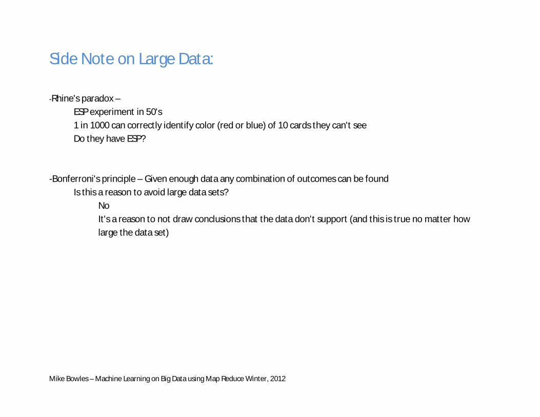
-Rhine's paradox – ESP experiment in 50's 1 in 1000 can correctly identify color (red or blue) of 10 cards they can't see Do they have ESP?
-Bonferroni's principle – Given enough data any combination of outcomes can be found
Is this a reason to avoid large data sets? No
It's a reason to not draw conclusions that the data don't support (and this is true no matter how large the data set)

Mike Bowles – Machine Learning on Big Data using Map Reduce Winter, 2012
Use Multiple Processor Cores
-What if we want to use the full data set? How can we devote more computational power to our job?
-There are always performance limits with a single processor core => Use multiple cores simulataneously.
-Traditional approach – add structure to programming language (C++, Java) -Issues with this approach
High communication costs (if data must be distributed over a network)
Difficult to deal with CPU failures at this level – (Processor failures are inevitable as scale increases) -To deal with these issues Google developed Map-Reduce Paradigm

Mike Bowles – Machine Learning on Big Data using Map Reduce Winter, 2012
What is Map-Reduce?
-Arrangement of compute tasks enabling relatively easy scaling. -Includes:
Hardware arrangement – racks of CPU's with direct access to local disk, networked to one another File System – Distributed storage across multiple disks, redundancy -Software processes running on various CPU in the assembly
Controller – manages mapper and reducer tasks, fault detection and recovery Mapper – Identical tasks assigned to multiple CPU's for each to run over its local data. Reducer – Aggregates output from several mappers to form end product
-Programmer only needs to author mapper and reducer. The rest of the structure is provided.
Dean, Jeff and Ghemawat, Sanjay. MapReduce: Simplified Data Processing on Large Clusters http://labs.google.com/papers/mapreduce-osdi04.pdf

Mike Bowles – Machine Learning on Big Data using Map Reduce Winter, 2012
Simple Code Example (using mrJob) – (this is running code) from mrjob.job import MRJob from math import sqrt import json class mrMeanVar(MRJob): DEFAULT_PROTOCOL = 'json' def mapper(self, key, line): num = json.loads(line) var = [num,num*num] yield 1,var def reducer(self, n, vars): N = 0.0 sum = 0.0 sumsq = 0.0 for x in vars: N += 1 sum += x[0] sumsq += x[1] mean = sum/N sd = sqrt(sumsq/N - mean*mean) results = [mean,sd] yield 1,results if __name__ == '__main__': mrMeanVar.run()
Mike Bowles – Machine Learning on Big Data using Map Reduce Winter, 2012
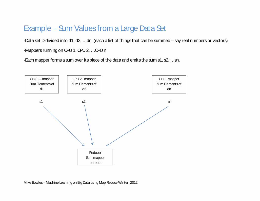
Example – Sum Values from a Large Data Set -Data set D divided into d1, d2, … dn (each a list of things that can be summed – say real numbers or vectors)
-Mappers running on CPU 1, CPU 2, … CPU n
-Each mapper forms a sum over its piece of the data and emits the sum s1, s2, … sn.
CPU 1 – mapper Sum Elements of
d1
CPU 2 - mapper Sum Elements of
d2
CPU - mapper Sum Elements of
dn
s1 s2 sn
Reducer Sum mapper
outputs

Mike Bowles – Machine Learning on Big Data using Map Reduce Winter, 2012
Machine Learning w. Map Reduce
-Statistical Query Model (see ref below) – A two-step process 1. Compute sufficient statistics by summing some functions over the data 2. Perform calculation on sums to yield data mining model 3. Conceptually similar to the "sum" example above.
-Consider ordinary least squares regression
Given m outputs yi (also called labels, observations, etc.) And m corresponding attribute vectors xi (also called regressors, predictors, etc.)
Fit a model of the form y = θT x by solving θ* = minθ ∑ (휃 푥 − 푦 )
Θ* = A-1 b where A = ∑ (푥 푥 ) and b = ∑ 푥 푦 -See the natural division into mapper and reducer? (Hint: Look for a ∑ ) Map-Reduce for Machine Learning on Multicore http://www.cs.stanford.edu/people/ang/papers/nips06-mapreducemulticore.pdf
Mike Bowles – Machine Learning on Big Data using Map Reduce Winter, 2012
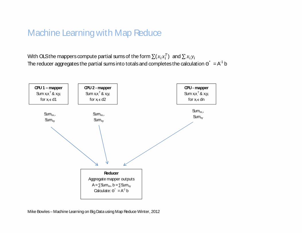
Machine Learning with Map Reduce With OLS the mappers compute partial sums of the form ∑(푥 푥 )and ∑푥 푦 The reducer aggregates the partial sums into totals and completes the calculation Θ* = A-1 b
CPU 1 – mapper Sum xix,
T & xiyi
for xi ϵ d1
CPU 2 - mapper Sum xix,
T & xiyi
for xi ϵ d2
CPU - mapper Sum xix,
T & xiyi
for xi ϵ dn
Sumxx,, Sumxy
Reducer Aggregate mapper outputs
A = ∑Sumxx, b = ∑Sumxy Calculate: Θ* = A-1 b
Sumxx,, Sumxy
Sumxx,, Sumxy

Mike Bowles – Machine Learning on Big Data using Map Reduce Winter, 2012
Machine Learning w. Map Reduce
-Referenced paper demonstrates that the following algorithms can all be arranged in this Statistical Query Model form:
Locally Weighted Linear Regression, Naïve Bayes, Gaussian Discriminative Analysis, k-Means, Neural Networks, Principal Component Analysis, Independent Component Analysis, Expectation Maximization, Support Vector Machines
-In some cases, iteration is required. Each iterative step involves a map-reduce sequence -Other machine learning algorithms can be arranged for map reduce – but not in Statistical Query Model form (e.g. canopy clustering or binary decision trees)

Mike Bowles – Machine Learning on Big Data using Map Reduce Winter, 2012
More Map Reduce Detail
-Mappers emit a key-value pair <key, value>
controller sorts key-value pairs <key, value> by key Reducer gets pairs grouped by key
-Mapper can be a two-step process
-With OLS, for example, we might have had the mapper emit each xixiT and xiyi, instead of emitting sums of
these quantities Post processing the mapper output (e.g. forming ∑ ) is a mapper function called "combiner" Reduces network traffic

Mike Bowles – Machine Learning on Big Data using Map Reduce Winter, 2012
Some Algorithms
-Canopy Cluster - -K-means -EM algo for Gaussian Mixture Model -Glmnet -SVM

Mike Bowles – Machine Learning on Big Data using Map Reduce Winter, 2012
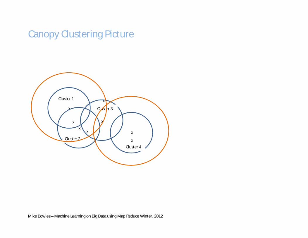
Canopy Clustering
-Usually used as rough clustering to reduce computation (e.g. search zip code for the closest pizza versus search the world) -Find well distributed initial conditions for other clustering also (e.g. kmeans) -Algorithm: Given set of points P and distance measure d(,) Pick two distance thresholds T1 > T2 > 0 Step 1: Find cluster centers
1. Initialize set of centers C = null 2. Iterate over points pi ϵ P
If there isn't c ϵ C s.t. d(c,pi) < T2 Add pi to C get next pi
Step 2: Assign point to clusters For pi ϵ P assign pi to {c ϵ C : d(pi , c) < T1} -Notice that points generally get assigned to more than one cluster. McCallum, Nigam, and Ungar "Efficient Clustering of High-Dimensional Data Sets with Application to Reference Matching", http://www.kamalnigam.com/papers/canopy-kdd00.pdf
Mike Bowles – Machine Learning on Big Data using Map Reduce Winter, 2012
Canopy Clustering Picture
x x
x
x
x
x
x
x
Cluster 1
Cluster 2
Cluster 3
Cluster 4

Mike Bowles – Machine Learning on Big Data using Map Reduce Winter, 2012
Canopy Clustering w Map Reduce
1st Pass – find centers
Mappers – Run canopy clustering on subset, pass centers to reducer Reducer – Run canopy clustering on centers from mappers.
2nd Pass – Make cluster assignments (if necessary)
Mappers – compare points pi to centers to form set ci = {c ϵ C | d(pi , c) < T1} Emit <key, value> = <c , pi > for each c ϵ ci
Reducer – Since the reducer input is sorted on key value (here, that's cluster center), the reducer input will be a list of all the points assigned to a given center.
-One small problem is that the centers picked by the reducer may not cover all the points of the combined original set. Pick T1 > 2*T2 or use larger T2 in reducer in order to insure that all points are covered. The Apache Mahout project has a lot of great algorithms and documentation. https://cwiki.apache.org/MAHOUT/canopy-clustering.html
Mike Bowles – Machine Learning on Big Data using Map Reduce Winter, 2012
K-Means Clustering
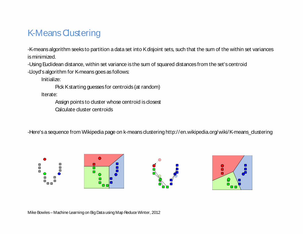
-K-means algorithm seeks to partition a data set into K disjoint sets, such that the sum of the within set variances is minimized. -Using Euclidean distance, within set variance is the sum of squared distances from the set's centroid -Lloyd's algorithm for K-means goes as follows: Initialize: Pick K starting guesses for centroids (at random) Iterate: Assign points to cluster whose centroid is closest Calculate cluster centroids -Here's a sequence from Wikipedia page on k-means clustering http://en.wikipedia.org/wiki/K-means_clustering

Mike Bowles – Machine Learning on Big Data using Map Reduce Winter, 2012
K-means in Map Reduce
Mapper – given K initial guesses, run through local data and for each point, determine which centroid is closest, accumulate vector sum of points closest to each centroid, combiner emits <centroidi , ( sumi , ni)> for each of the i centroids. Reducer – for each old centroidi , aggregate sum and n from all mappers and calculate new centroid. This map-reduce pair completes an iteration of Lloyd's algorithm.

Mike Bowles – Machine Learning on Big Data using Map Reduce Winter, 2012
Support Vector Machine - SVM
-For classification, SVM finds separating hyperplane -H3 does not separate classes. H1 separates, but not with max margin. H2 separates with max margin Figure from http://en.wikipedia.org/wiki/Support_vector_machine

Mike Bowles – Machine Learning on Big Data using Map Reduce Winter, 2012
SVM as Mathematical Optimization Problem
-Given a training set S = {(푥 , 푦 )} -Where xi ϵ Rn and yi ϵ { +1, -1} -We can write any linear functional of x as wTx +b, where w ϵ Rn and b is scalar Find weight vector w and constant b to minimize
푚푖푛 , 12||푤|| +
퐶푚 푙(푤, 푏; (푥,푦))
( , )∈
Where l(w,b;(x,y)) = max{0, 1 – y (wTx + b)}

Mike Bowles – Machine Learning on Big Data using Map Reduce Winter, 2012
Solution by Batch Gradient Descent -We can solve this by using batch gradient descent. Take a derivative wrt w & b. Notice that if the 1 - y (wTx + b) < 0, then l() = 0 and∇ , 푙( ) = 0. Denote by S+ = {(x,y) ϵ S | 1 - y (wTx + b) > 0 }. Then the gradient wrt w is
w + ∑ −푦푥( , )∈
and wrt b is:
∑ −푦( , )∈ For reference see "Map Reduce for Machine Learning on Multicore" mentioned earlier. Also see Shalev-Shwartz, "Pegasos: Primal Estimated sub-Gradient Solver for SVM"

Mike Bowles – Machine Learning on Big Data using Map Reduce Winter, 2012
Calculating a Gradient Step
-What's important about what we just developed? Several things
1. In the equation we wound up with terms like (w + ∑ −푦푥( , )∈ ), only the term inside the sum is
data dependent. 2. The data dependent terms sum(-yx) is summed over the points in the input data where the constraints
are active. -Let's summarize by drawing up the mapper and reducer functions. Initialize w and b, C and m (# of instances). Iterate Mapper – Each mapper has access to a subset Sm of S. For points (x,y) ϵ Sm check 1 - y (wTx + b) > 0. If yes, accumulate – y and – yx. Emit <,(∑-y, ∑ -yx)>. We'll put in a dummy key value, but all the output gets summarized in a single (vector) quantity to be processed by a single reducer Reducer – Accumulate ∑-y and ∑ -yx and update estimate of w and b using
wnew = wold - ϵ (wold + ∑-yx)
and
bnew = bold - ϵ ( ∑-y)

Mike Bowles – Machine Learning on Big Data using Map Reduce Winter, 2012
GLMNet Algorithm -Regularized Regression -To avoid over-fitting have to exert control over degrees of freedom in regression -cut back on attributes – subset selection -penalize regression coefficients – coefficient shrinkage, ridge regression, lasso regression -With Coefficient Shrinkage, different penalties give solutions with different properties "Regularization Paths for Generalized Linear Models, via Coordinate Descent" Friedman, Hastie and Tibshirani http://www.stanford.edu/~hastie/Papers/glmnet.pdf

Mike Bowles – Machine Learning on Big Data using Map Reduce Winter, 2012
Regularizing Regression with Coefficient Shrinkage -Start with OLS problem formulation and add a penalty to OLS error -Suppose
y ϵ R and vector of predictors x ϵ Rn -As with OLS, seek a fit for y of the form
y ≈ β0 + xTβ -Assume that xi have been standardized to mean zero and unit variance -Find
푚푖푛( , ) ∑ 푦 −훽 −푥 훽 + 휋푃 (훽)
-The part in the sum is the ordinary least squares penalty. The bit at the end (휋푃 (훽)) is new. -Notice that the minimizing set of β's is a function of the parameter π. If π = 0 we get OLS coefficients.

Mike Bowles – Machine Learning on Big Data using Map Reduce Winter, 2012
Penalty Term -The coefficient penalty term is given by
Pα(β) = ∑ (1 − 훼)훽 + 훼|훽 |
-This is called "elasticnet" penalty (see ref below).
- α = 1 gives l1 penalty (sum of absolute values) - α = 0 gives l2 – squared penalty (sum of squares)
-Why is this important? The choice of penalty influences that nature of the solutions. l1 gives sparse solutions. It ignores attributes. l2 tends to average correlated attributes. -Consider the coefficient paths as functions of the parameter π. H. Zou and T. Hastie. Regularization and variable selection via the elastic net. J. Royal. Stat. Soc. B., 67(2):301{320, 2005.

Mike Bowles – Machine Learning on Big Data using Map Reduce Winter, 2012
Coefficient Trajectories -Here's Figure 1 from Friedman et. al. paper

Mike Bowles – Machine Learning on Big Data using Map Reduce Winter, 2012
Pathwise Solution -This algorithm works as follows: Initialize with value of π large enough that all β's are 0. Decrease π slightly and update β's by taking a gradient step from the old β based on new value of π. Small changes in π means that the update converges quickly. In many cases faster to generate entire coefficient trajectory with this algo, than to generate point solution -Friedman et. al. show that the elements of the coefficient vector βj satisfies
βj = ∑ ( ) ,
( )
where the function S() is given by S(z,γ) = z – γ if z > 0 and γ < |z| = z + γ if z < 0 and γ < |z| = 0 if γ >= |z| -The point is:
This algorithm fits the Statistical Query Model. The sum inside the function S() can be spread over any number of mappers This algorithm handles elasticnet regularized regressions, logistic regression and multiclass logistic
regression

Mike Bowles – Machine Learning on Big Data using Map Reduce Winter, 2012
Summary -Here's what we covered 1. Where do big-data machine learning problems arise? -e-commerce, retail, narrow targeting, bank and credit cards 2. What ways are there to deal with big-data machine learning problems? -sample, language level parallelization, map-reduce 3. What is map-reduce? -programming formalism that isolates programming task to mapper and reducer functions 3. Application of map-reduce to some familiar machine learning algorithms
Hope you learned something from the class. To get into more detail, come to the big-data class.