• Today: isostasy and Earth rheology, paper discussion
• Next week: sea level and glacial isostatic adjustment
• Email – did you get my email today?
• Class notes, website
• Your presentations: – November 3rd and 10th
– 30 minutes each, plus additional time for questions– Individual or in pairs (say what each contributed if in pairs)– 40% of final grade
Course Business

• Required elements (90% of grade):– Reference list, including foundational and most recent work (the
references you would include in the introduction section to a paper that will be reviewed by experts in the field)
– Discussion of relevant data, models, physical processes at play, and methods of analysis
– Slides (turn in a PDF and any auxilliary files)– Optional: your own analysis
• Feedback (10% of grade): You will be asked to give written positive and constructive feedback for each presentation. We will collect your feedback forms, grade the quality of the feedback, and then pass it on to the presenters along with our own feedback. (Giving useful feedback is an essential life skill – I encourage you to read up on how to do it well before the presentations start)
• You will be assessed on the content and quality (clarity, structure, use of visuals, engagement of the audience, etc.) of your presentatio
Presentations
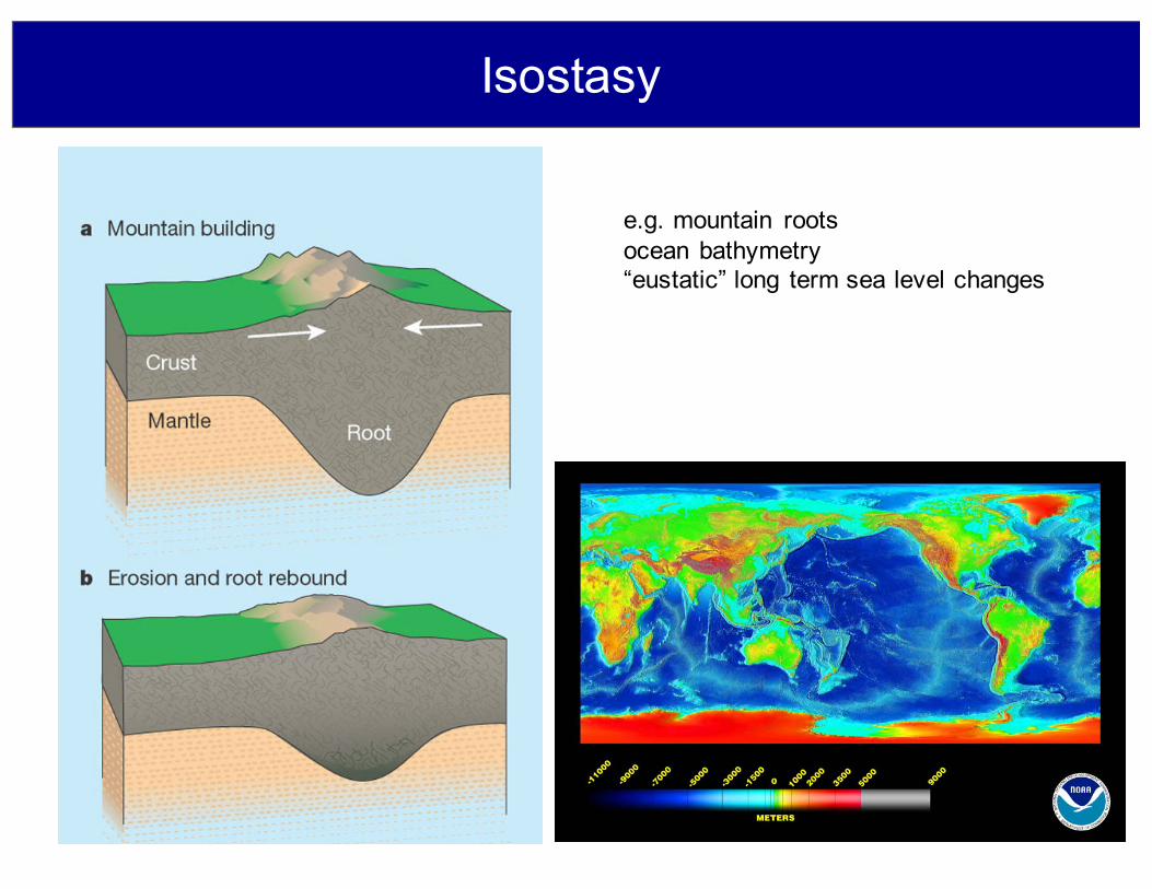
Isostasy
e.g. mountain rootsocean bathymetry “eustatic” long term sea level changes
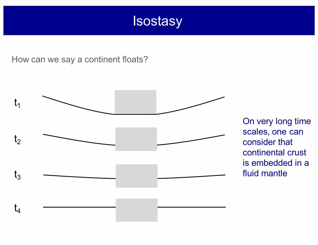
How can we say a continent floats?
t1
t2
t3
t4
On very long time scales, one can consider that continental crust is embedded in a fluid mantle
Isostasy

Now, treat the continent as a block of wood floating on a sea of mantle rock:
h
AWhat is the equilibrium position of the continent?
ρcb
Isostasy
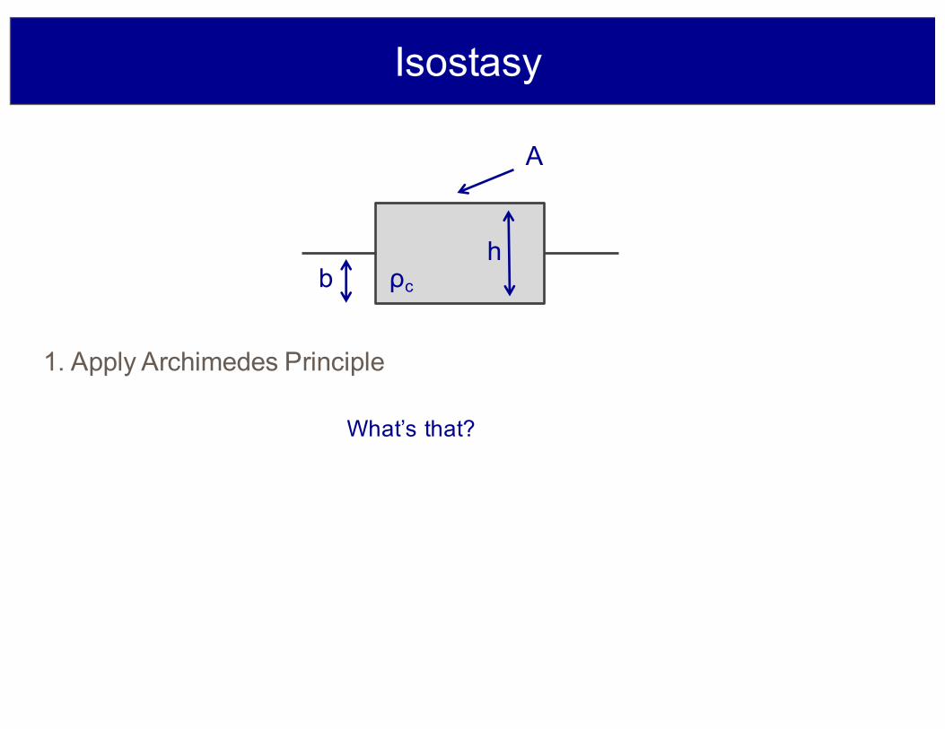
1. Apply Archimedes Principle
h
A
What’s that?
ρcb
Isostasy

1. Apply Archimedes Principle
h
A
Buoyancy force on material = weight of material it displaces
ρcb
Jerry Mitrovica
⇥Ag (1)
⇤yyA = ⇥ ⌅Ag (2)
⇤yy = ⇥ ⌅g (3)
�A (4)
⇥m (5)
⇥c (6)
⇥chAg = ⇥mbAg (7)
b
h=
⇥c⇥m
(8)
h� b = h
1� ⇥c
⇥m
�(9)
⇥c ! ⇥m (10)
h� b ! 0 (11)
⇥m >> ⇥c (12)
b ! 0 (13)
⇥chg = ⇥mbg (14)
⇥chAg + ⇥m(D � b)Ag (15)
⇥mDAg (16)
⇥chAg + ⇥m(D � b)Ag = ⇥mDAg (17)
⇥ch+ ⇥m(D � b) = ⇥mD (18)
1
Jerry Mitrovica
⇥Ag (1)
⇤yyA = ⇥ ⌅Ag (2)
⇤yy = ⇥ ⌅g (3)
�A (4)
⇥m (5)
⇥c (6)
⇥chAg = ⇥mbAg (7)
b
h=
⇥c⇥m
(8)
h� b = h
1� ⇥c
⇥m
�(9)
⇥c ! ⇥m (10)
h� b ! 0 (11)
⇥m >> ⇥c (12)
b ! 0 (13)
⇥chg = ⇥mbg (14)
⇥chAg + ⇥m(D � b)Ag (15)
⇥mDAg (16)
⇥chAg + ⇥m(D � b)Ag = ⇥mDAg (17)
⇥ch+ ⇥m(D � b) = ⇥mD (18)
1
Jerry Mitrovica
⇥Ag (1)
⇤yyA = ⇥ ⌅Ag (2)
⇤yy = ⇥ ⌅g (3)
�A (4)
⇥m (5)
⇥c (6)
⇥chAg = ⇥mbAg (7)
b
h=
⇥c⇥m
(8)
h� b = h
1� ⇥c
⇥m
�(9)
⇥c ! ⇥m (10)
h� b ! 0 (11)
⇥m >> ⇥c (12)
b ! 0 (13)
⇥chg = ⇥mbg (14)
⇥chAg + ⇥m(D � b)Ag (15)
⇥mDAg (16)
⇥chAg + ⇥m(D � b)Ag = ⇥mDAg (17)
⇥ch+ ⇥m(D � b) = ⇥mD (18)
1
Isostasy
Jerry Mitrovica
⇥Ag (1)
⇤yyA = ⇥ ⌅Ag (2)
⇤yy = ⇥ ⌅g (3)
�A (4)
⇥m (5)
⇥c (6)
⇥chAg = ⇥mbAg (7)
b
h=
⇥c⇥m
(8)
h� b = h
1� ⇥c
⇥m
�(9)
⇥c ! ⇥m (10)
h� b ! 0 (11)
⇥m >> ⇥c (12)
b ! 0 (13)
⇥chg = ⇥mbg (14)
⇥chAg + ⇥m(D � b)Ag (15)
⇥mDAg (16)
⇥chAg + ⇥m(D � b)Ag = ⇥mDAg (17)
⇥ch+ ⇥m(D � b) = ⇥mD (18)
1
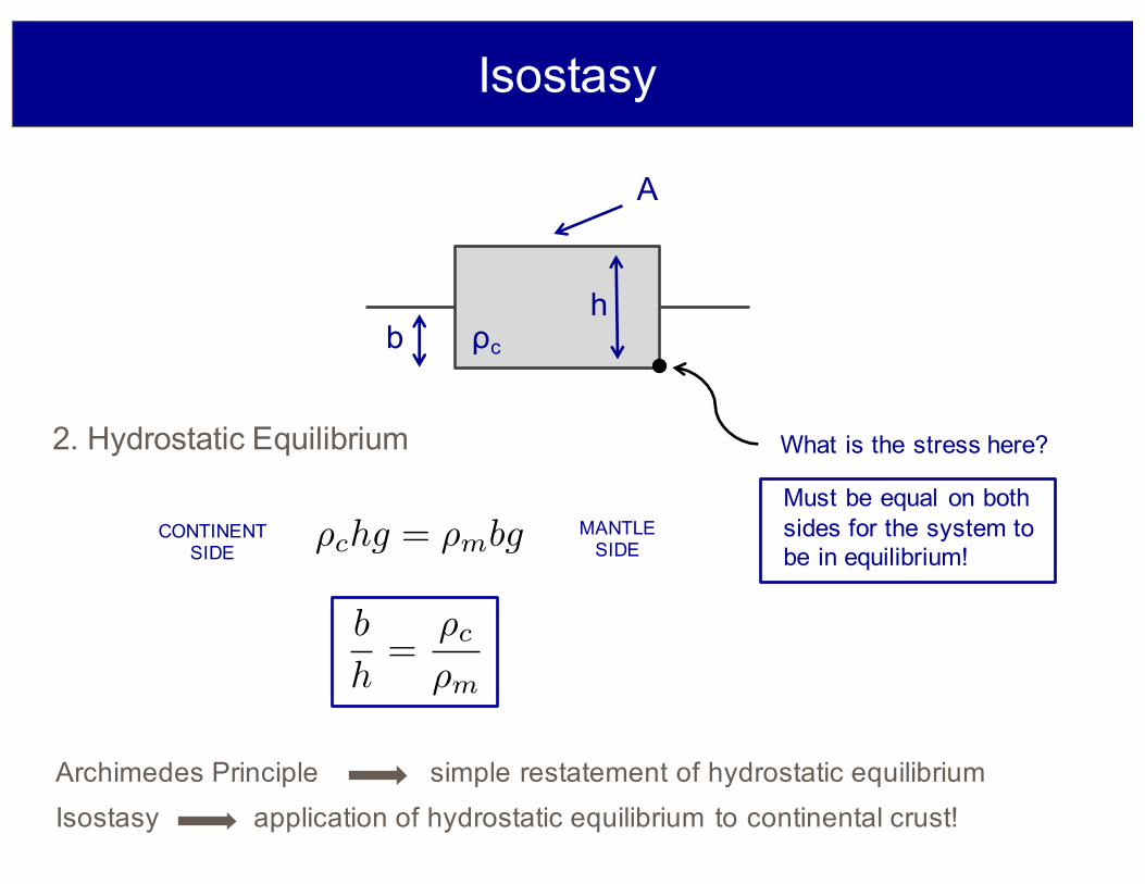
2. Hydrostatic Equilibrium
h
A
What is the stress here?
ρcb
Must be equal on both sides for the system to be in equilibrium!
Jerry Mitrovica
⇥Ag (1)
⇤yyA = ⇥ ⌅Ag (2)
⇤yy = ⇥ ⌅g (3)
�A (4)
⇥m (5)
⇥c (6)
⇥chAg = ⇥mbAg (7)
b
h=
⇥c⇥m
(8)
h� b = h
1� ⇥c
⇥m
�(9)
⇥c ! ⇥m (10)
h� b ! 0 (11)
⇥m >> ⇥c (12)
b ! 0 (13)
⇥chg = ⇥mbg (14)
⇥chAg + ⇥m(D � b)Ag (15)
⇥mDAg (16)
⇥chAg + ⇥m(D � b)Ag = ⇥mDAg (17)
⇥ch+ ⇥m(D � b) = ⇥mD (18)
1
CONTINENTSIDE
MANTLESIDE
Archimedes Principle simple restatement of hydrostatic equilibriumIsostasy application of hydrostatic equilibrium to continental crust!
Isostasy

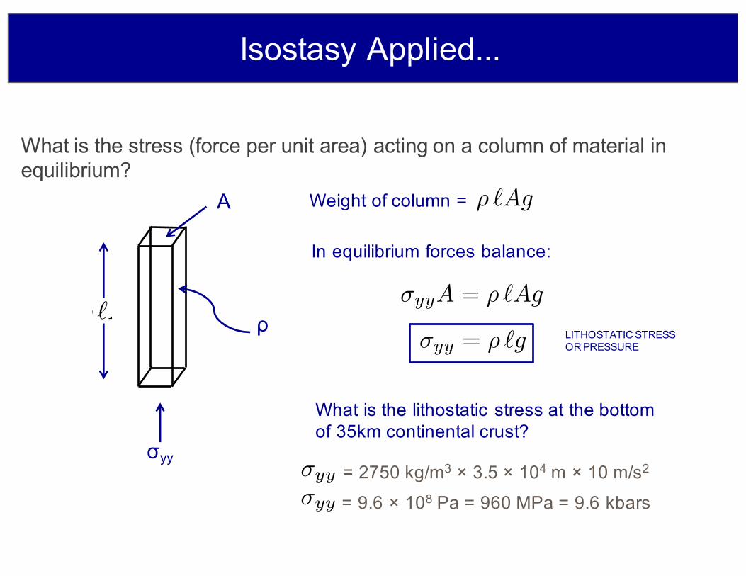
What is the stress (force per unit area) acting on a column of material in equilibrium?
σyy
Lρ
A
Isostasy
What is the stress (force per unit area) acting on a column of material in equilibrium?
σyy
ρ
A Weight of column =
In equilibrium forces balance:
What is the lithostatic stress at the bottom of 35km continental crust?
LITHOSTATIC STRESSOR PRESSURE
= 2750 kg/m3 × 3.5 × 104 m × 10 m/s2
= 9.6 × 10⁸ Pa = 960 MPa = 9.6 kbars
Jerry Mitrovica
⇥Ag (1)
⇤yyA = ⇥ ⌅Ag (2)
⇤yy = ⇥ ⌅g (3)
�A (4)
⇥m (5)
⇥c (6)
⇥chAg = ⇥mbAg (7)
b
h=
⇥c⇥m
(8)
h� b = h
1� ⇥c
⇥m
�(9)
⇥c ! ⇥m (10)
h� b ! 0 (11)
⇥m >> ⇥c (12)
b ! 0 (13)
⇥chg = ⇥mbg (14)
⇥chAg + ⇥m(D � b)Ag (15)
⇥mDAg (16)
⇥chAg + ⇥m(D � b)Ag = ⇥mDAg (17)
⇥ch+ ⇥m(D � b) = ⇥mD (18)
1
Jerry Mitrovica
⇥Ag (1)
⇤yyA = ⇥ ⌅Ag (2)
⇤yy = ⇥ ⌅g (3)
�A (4)
⇥m (5)
⇥c (6)
⇥chAg = ⇥mbAg (7)
b
h=
⇥c⇥m
(8)
h� b = h
1� ⇥c
⇥m
�(9)
⇥c ! ⇥m (10)
h� b ! 0 (11)
⇥m >> ⇥c (12)
b ! 0 (13)
⇥chg = ⇥mbg (14)
⇥chAg + ⇥m(D � b)Ag (15)
⇥mDAg (16)
⇥chAg + ⇥m(D � b)Ag = ⇥mDAg (17)
⇥ch+ ⇥m(D � b) = ⇥mD (18)
1
Jerry Mitrovica
⇥Ag (1)
⇤yyA = ⇥ ⌅Ag (2)
⇤yy = ⇥ ⌅g (3)
�A (4)
⇥m (5)
⇥c (6)
⇥chAg = ⇥mbAg (7)
b
h=
⇥c⇥m
(8)
h� b = h
1� ⇥c
⇥m
�(9)
⇥c ! ⇥m (10)
h� b ! 0 (11)
⇥m >> ⇥c (12)
b ! 0 (13)
⇥chg = ⇥mbg (14)
⇥chAg + ⇥m(D � b)Ag (15)
⇥mDAg (16)
⇥chAg + ⇥m(D � b)Ag = ⇥mDAg (17)
⇥ch+ ⇥m(D � b) = ⇥mD (18)
1
Jerry Mitrovica
⇥Ag (1)
⇤yyA = ⇥ ⌅Ag (2)
⇤yy = ⇥ ⌅g (3)
�A (4)
⇥m (5)
⇥c (6)
⇥chAg = ⇥mbAg (7)
b
h=
⇥c⇥m
(8)
h� b = h
1� ⇥c
⇥m
�(9)
⇥c ! ⇥m (10)
h� b ! 0 (11)
⇥m >> ⇥c (12)
b ! 0 (13)
⇥chg = ⇥mbg (14)
⇥chAg + ⇥m(D � b)Ag (15)
⇥mDAg (16)
⇥chAg + ⇥m(D � b)Ag = ⇥mDAg (17)
⇥ch+ ⇥m(D � b) = ⇥mD (18)
1
Jerry Mitrovica
⇥Ag (1)
⇤yyA = ⇥ ⌅Ag (2)
⇤yy = ⇥ ⌅g (3)
�A (4)
⇥m (5)
⇥c (6)
⇥chAg = ⇥mbAg (7)
b
h=
⇥c⇥m
(8)
h� b = h
1� ⇥c
⇥m
�(9)
⇥c ! ⇥m (10)
h� b ! 0 (11)
⇥m >> ⇥c (12)
b ! 0 (13)
⇥chg = ⇥mbg (14)
⇥chAg + ⇥m(D � b)Ag (15)
⇥mDAg (16)
⇥chAg + ⇥m(D � b)Ag = ⇥mDAg (17)
⇥ch+ ⇥m(D � b) = ⇥mD (18)
1
Jerry Mitrovica
⇥Ag (1)
⇤yyA = ⇥ ⌅Ag (2)
⇤yy = ⇥ ⌅g (3)
�A (4)
⇥m (5)
⇥c (6)
⇥chAg = ⇥mbAg (7)
b
h=
⇥c⇥m
(8)
h� b = h
1� ⇥c
⇥m
�(9)
⇥c ! ⇥m (10)
h� b ! 0 (11)
⇥m >> ⇥c (12)
b ! 0 (13)
⇥chg = ⇥mbg (14)
⇥chAg + ⇥m(D � b)Ag (15)
⇥mDAg (16)
⇥chAg + ⇥m(D � b)Ag = ⇥mDAg (17)
⇥ch+ ⇥m(D � b) = ⇥mD (18)
1
Isostasy Applied...

3. Isostasy in Geophysics
hρcb
Isostasy: The total mass in any vertical column through the crust must be equal no matter where the column is (when in isostatic equilibrium)
Depth ofCompensation
Column 1 Weight:
Column 2 Weight:
Equate:
Jerry Mitrovica
⇥Ag (1)
⇤yyA = ⇥ ⌅Ag (2)
⇤yy = ⇥ ⌅g (3)
�A (4)
⇥m (5)
⇥c (6)
⇥chAg = ⇥mbAg (7)
b
h=
⇥c⇥m
(8)
h� b = h
1� ⇥c
⇥m
�(9)
⇥c ! ⇥m (10)
h� b ! 0 (11)
⇥m >> ⇥c (12)
b ! 0 (13)
⇥chg = ⇥mbg (14)
⇥chAg + ⇥m(D � b)Ag (15)
⇥mDAg (16)
⇥chAg + ⇥m(D � b)Ag = ⇥mDAg (17)
⇥ch+ ⇥m(D � b) = ⇥mD (18)
1
Jerry Mitrovica
⇥Ag (1)
⇤yyA = ⇥ ⌅Ag (2)
⇤yy = ⇥ ⌅g (3)
�A (4)
⇥m (5)
⇥c (6)
⇥chAg = ⇥mbAg (7)
b
h=
⇥c⇥m
(8)
h� b = h
1� ⇥c
⇥m
�(9)
⇥c ! ⇥m (10)
h� b ! 0 (11)
⇥m >> ⇥c (12)
b ! 0 (13)
⇥chg = ⇥mbg (14)
⇥chAg + ⇥m(D � b)Ag (15)
⇥mDAg (16)
⇥chAg + ⇥m(D � b)Ag = ⇥mDAg (17)
⇥ch+ ⇥m(D � b) = ⇥mD (18)
1
Jerry Mitrovica
⇥Ag (1)
⇤yyA = ⇥ ⌅Ag (2)
⇤yy = ⇥ ⌅g (3)
�A (4)
⇥m (5)
⇥c (6)
⇥chAg = ⇥mbAg (7)
b
h=
⇥c⇥m
(8)
h� b = h
1� ⇥c
⇥m
�(9)
⇥c ! ⇥m (10)
h� b ! 0 (11)
⇥m >> ⇥c (12)
b ! 0 (13)
⇥chg = ⇥mbg (14)
⇥chAg + ⇥m(D � b)Ag (15)
⇥mDAg (16)
⇥chAg + ⇥m(D � b)Ag = ⇥mDAg (17)
⇥ch+ ⇥m(D � b) = ⇥mD (18)
1
Jerry Mitrovica
⇥Ag (1)
⇤yyA = ⇥ ⌅Ag (2)
⇤yy = ⇥ ⌅g (3)
�A (4)
⇥m (5)
⇥c (6)
⇥chAg = ⇥mbAg (7)
b
h=
⇥c⇥m
(8)
h� b = h
1� ⇥c
⇥m
�(9)
⇥c ! ⇥m (10)
h� b ! 0 (11)
⇥m >> ⇥c (12)
b ! 0 (13)
⇥chg = ⇥mbg (14)
⇥chAg + ⇥m(D � b)Ag (15)
⇥mDAg (16)
⇥chAg + ⇥m(D � b)Ag = ⇥mDAg (17)
⇥ch+ ⇥m(D � b) = ⇥mD (18)
1
Jerry Mitrovica
⇥Ag (1)
⇤yyA = ⇥ ⌅Ag (2)
⇤yy = ⇥ ⌅g (3)
�A (4)
⇥m (5)
⇥c (6)
⇥chAg = ⇥mbAg (7)
b
h=
⇥c⇥m
(8)
h� b = h
1� ⇥c
⇥m
�(9)
⇥c ! ⇥m (10)
h� b ! 0 (11)
⇥m >> ⇥c (12)
b ! 0 (13)
⇥chg = ⇥mbg (14)
⇥chAg + ⇥m(D � b)Ag (15)
⇥mDAg (16)
⇥chAg + ⇥m(D � b)Ag = ⇥mDAg (17)
⇥ch+ ⇥m(D � b) = ⇥mD (18)
1
Isostasy Applied...

Application to Cooling of the Oceanic Lithosphere and Ocean Bathymetry
Isostasy Applied...
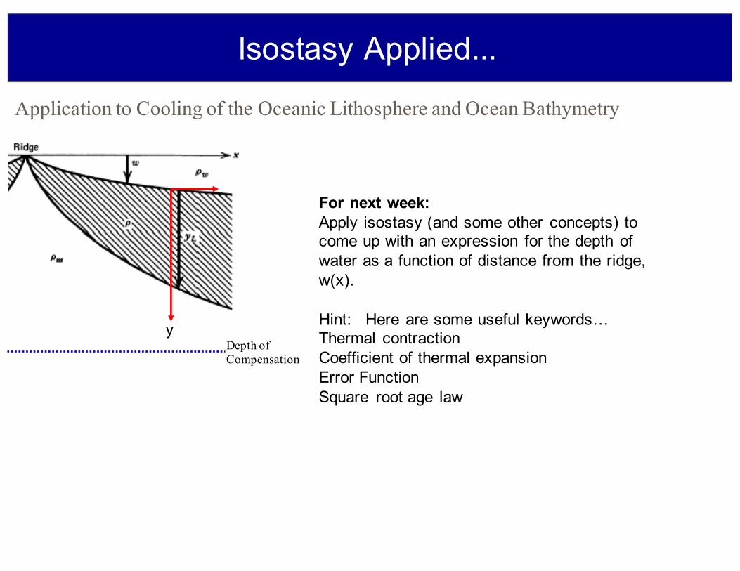
yDepth ofCompensation
Application to Cooling of the Oceanic Lithosphere and Ocean Bathymetry
For next week: Apply isostasy (and some other concepts) to come up with an expression for the depth of water as a function of distance from the ridge, w(x).
Hint: Here are some useful keywords…Thermal contractionCoefficient of thermal expansionError FunctionSquare root age law
Isostasy Applied...

Isostasy Applied...
At the Last Glacial Maximum (LGM), ~ 20 ky ago, ~3 km of ice covered North America. Assuming the continent is close to isostatic equilibrium today, how much lower was Montreal at the LGM?
LGM Modern

But! North America is not in isostatic equilibrium! [ still O(100 m) of rebound to go ]
Isostasy Applied...
GPS vertical velocities from Sella et al. (2007)

We may come back to isostasy in the context of discussing long term sea level over timescales of millions of years and longer. Topics here include: - cautionary tales in sequence stratigraphy- interpreting the Exxon Vail Curves as “eustatic”- changes in sea level caused by changes in tectonic
plate spreading rates, continental collisions, dynamic topography, …
But for now, on to Earth rheology on shorter timescales.
Isostasy Applied...

t1
t2
t3
t4
Isostasy à Rheology
“T’ain’t what you do it, it’s the way that you do it.”Written by Melvin Oliver and James Young (1939),
first sung on recording by Ella Fitzgerald

Fapp
M
What happens?
Elastic
Viscous
Viscoelastic
Rheology: The macroscopic response of a material to stress (applied forcing)
Brittle
What is the Earth’s rheology?
Why does it matter?
Earth Rheology
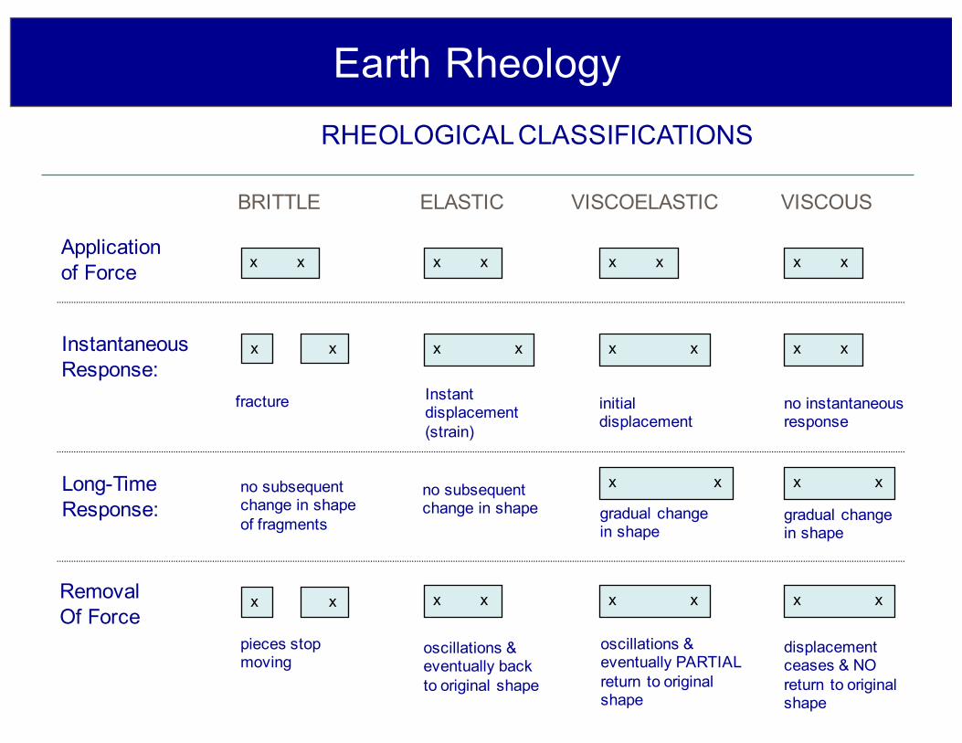
RHEOLOGICAL CLASSIFICATIONS
Applicationof Force
RemovalOf Force
BRITTLE ELASTIC VISCOELASTIC VISCOUS
x x x x x x x x
x x x x x x x xInstantaneousResponse:
Long-TimeResponse:
fracture Instantdisplacement(strain)
initialdisplacement
no instantaneousresponse
no subsequentchange in shape of fragments
no subsequentchange in shape gradual change
in shape gradual changein shape
x x x x
x x x x x x x x
pieces stopmoving
oscillations &eventually backto original shape
oscillations &eventually PARTIALreturn to original shape
displacementceases & NOreturn to original shape
Earth Rheology

1-D MODELS OF RHEOLOGY
Stress: force/unit area FStrain: δlength/length e
1) Elastic spring:
F
L
Hooke’s Law states:
Stress is proportional to strain & constant of proportionality‘k’ is spring constant (called “Young’s modulus” in materials)
Earth Rheology

1-D MODELS OF RHEOLOGY
2) Viscous Dashpot
L
F
Pot filled with viscous fluid & piston
Newtonian fluid:
Stress is proportional to strain rate & constant of proportionality‘η’ is coefficient of viscosity (units: Pa s = N m-2s)
Earth Rheology

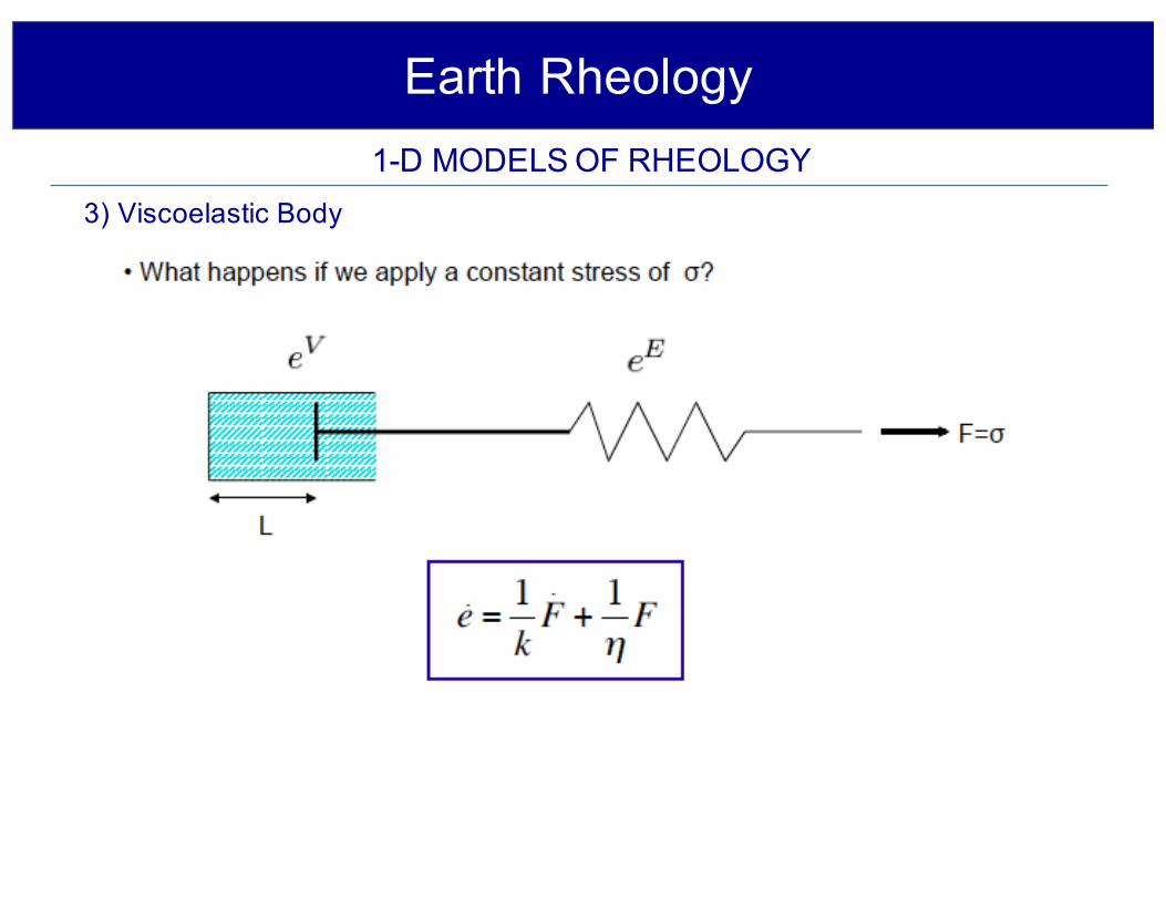
1-D MODELS OF RHEOLOGY3) Viscoelastic Body
L
F
• many ways to define such a material• assume the following 1-D linear response: “Maxwell Body”
Physics?
Earth Rheology

1-D MODELS OF RHEOLOGY3) Viscoelastic Body
L
F
• many ways to define such a material• assume the following 1-D linear response: “Maxwell Body”
• application of stress yields immediate elastic (E) response and a subsequent viscous (v) response
How are stresses on each element related? What is the total strain?
Earth Rheology

1-D MODELS OF RHEOLOGY3) Viscoelastic Body
L
F
• many ways to define such a material• assume the following 1-D linear response: “Maxwell Body”
• application of stress yields immediate elastic (E) response and a subsequent viscous (v) response:
Constitutive equation (i.e. equation relating stress & strain) for a Maxwell viscoelastic 1-D body
. .
Earth Rheology

1-D MODELS OF RHEOLOGY3) Viscoelastic Body
L
F
• many ways to define such a material• assume the following 1-D linear response: “Maxwell Body”
• constitutive equation:
. .
End members: Viscous bodyElastic body
Earth Rheology
1-D MODELS OF RHEOLOGY3) Viscoelastic Body
Earth Rheology

1-D MODELS OF RHEOLOGY3) Viscoelastic Body
Earth Rheology

1-D MODELS OF RHEOLOGY3) Viscoelastic Body
Earth Rheology

1-D MODELS OF RHEOLOGY3) Viscoelastic Body
Earth Rheology

1-D MODELS OF RHEOLOGY3) Viscoelastic Body
L
F
. .
• What happens if we apply a constant strain of at
Earth Rheology

• constitutive equation relates stress & strain• in our examples: 1-D elastic, viscous, or Maxwell (linear) viscoelastic• in general, require 3-D formulation for Earth’s response --> tensor algebra
(e.g. Hooke’s Law in 3-D)• viscoelastic rheology need not be linear, i.e.,• Complications (and the exciting part!!): a single type of material can
behave as a brittle, elastic, viscoelastic or viscous body depending on:
RHEOLOGICAL CLASSIFICATIONS
.
• Pressure• Temperature• Force Magnitude• Force Duration
Physical Environment
Material rheology depends on P, T, FM,FD
e.g., silly putty, tar, glass
Nature of Applied Forcing
Earth Rheology
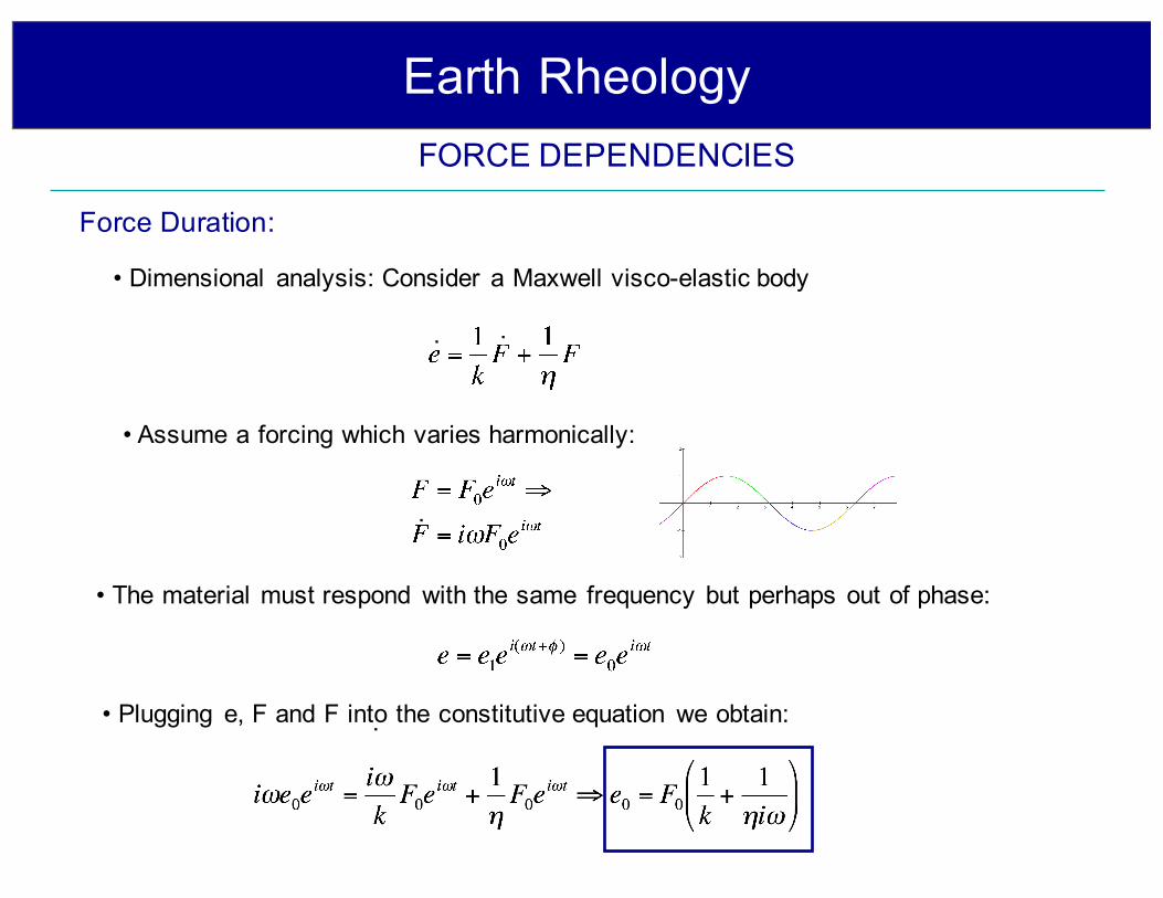
FORCE DEPENDENCIES
• Dimensional analysis: Consider a Maxwell visco-elastic body
• Assume a forcing which varies harmonically:
.
• The material must respond with the same frequency but perhaps out of phase:
• Plugging e, F and F into the constitutive equation we obtain:.
Force Duration:
. .
Earth Rheology

FORCE DEPENDENCIES
(A) Short-time scale forces: Elastic response
(B) Long-time scale forces: Viscous response
(C) Intermediate time scale forces: visco-elastic response - body can behave as a ‘fluid’ or a ‘solid’ depending on the time scale of the applied forcing
• The Earth has different rheological responses to different forcings•Seismic, tides: Elastic•Wobble, post-glacial rebound, polar wander: Visco-elastic•Convection: viscous
• By studying these forcings and the Earth’s response to them, we can determine information on the Earth’s interior
Force Duration:
.
Earth Rheology

THE EARTH AS A VISCOUS SOLID!
.
MAXWELL TIME
t (seconds)104100 108 10161012
free oscillations tides wobble
Glacialisostatic
adjustmentmantle
convection
• The Earth has different rheological responses to different forcings• By studying these forcings and the Earth’s response to them, we can
determine information on the Earth’s interior
Earth Rheology

Cases:(1) Cold … means η large so:
(2) Hot … means η small so:
(3) Warm … intermediate T so: viscoelastic response … similar to tar
ENVIRONMENT DEPENDENCIES.
• Both k & η are functions of pressure P & temperature T
• ν is a much stronger function of P,T (in general)
• to a first approximation:
• experiments have shown:
• “a” is a complex function of thermodynamic properties
• thus, small changes in temperature produce exponentially large changes in viscosity!!!
.
. .
Elastic response
.
.
Viscous response
.
.
Earth Rheology
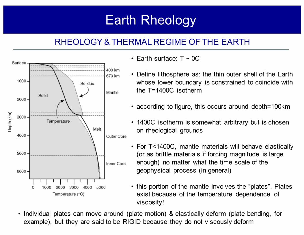
RHEOLOGY & THERMAL REGIME OF THE EARTH
• Earth surface: T ~ 0C
• Define lithosphere as: the thin outer shell of the Earth whose lower boundary is constrained to coincide with the T=1400C isotherm
• according to figure, this occurs around depth=100km
• 1400C isotherm is somewhat arbitrary but is chosen on rheological grounds
• For T<1400C, mantle materials will behave elastically (or as brittle materials if forcing magnitude is large enough) no matter what the time scale of the geophysical process (in general)
• this portion of the mantle involves the “plates”. Plates exist because of the temperature dependence of viscosity!
• Individual plates can move around (plate motion) & elastically deform (plate bending, for example), but they are said to be RIGID because they do not viscously deform
Earth Rheology

• To understand questions like: What is a plate?Why does it exist?What drives the plates?
we require knowledge of the Earth’s rheological behaviour
• Rheology of Earth materials tells us how Earth responds to forcings associated with:
Forcing: Response:•Large earthquakes ---> seismic waves•Gravitational pull of the sun and moon ---> tides•Melting of glaciers ---> post-glacial rebound•Temperature contrast between
CMB & surface + internal heating ---> mantle convection
• These forcings have a wide range of characteristic time scales• We can observe the responses and use this information to constrain elastic and
viscous properties of the Earth’s interior• examples: seismology tells us about the Earth’s elastic structure
post-glacial rebound tells us about the Earth’s viscosity profile
Why we care

•Free oscillations (earth ringing due to forcing like an earthquake)
Seismology

•Body wave data (track paths of seismic rays through Earth)
Preliminary Reference Earth Model“PREM” gives density and seismic
wave speeds as a function of radius-wave speeds related to Young’s
modulus (elastic property)
Seismology
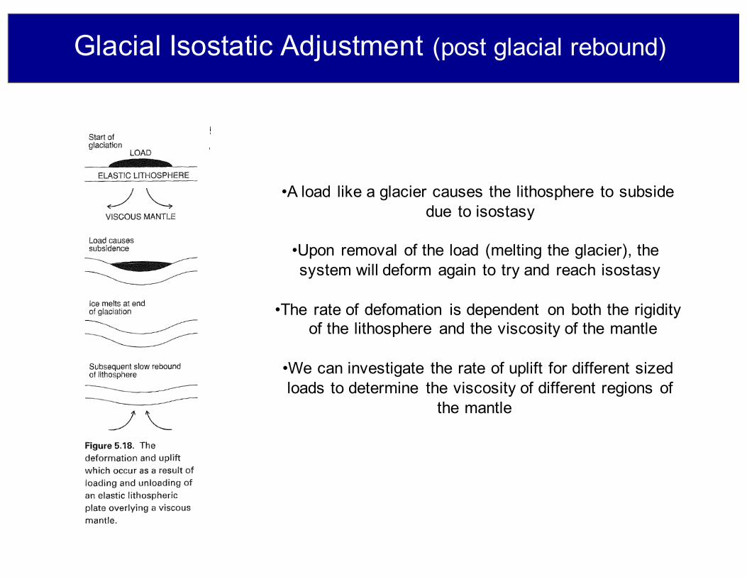
•A load like a glacier causes the lithosphere to subsidedue to isostasy
•Upon removal of the load (melting the glacier), the system will deform again to try and reach isostasy
•The rate of defomation is dependent on both the rigidityof the lithosphere and the viscosity of the mantle
•We can investigate the rate of uplift for different sizedloads to determine the viscosity of different regions of
the mantle
Glacial Isostatic Adjustment (post glacial rebound)