LEARNING ENERGY-BASED APPROXIMATE
INFERENCE NETWORKS
FOR STRUCTURED APPLICATIONS IN NLP
Lifu Tu
August 2021
A DISSERTATION SUBMITTED AT
TOYOTA TECHNOLOGICAL INSTITUTE AT CHICAGO
IN PARTIAL FULFILLMENT OF THE REQUIREMENTS
FOR THE DEGREE OF
DOCTOR OF PHILOSOPHY IN COMPUTER SCIENCE
Thesis Committee:
Kevin Gimpel (Thesis Advisor)
Karen Livescu
Sam Wiseman
Kyunghyun Cho
Marc’Aurelio Ranzato
arX
iv:2
108.
1252
2v1
[cs
.CL
] 2
7 A
ug 2
021

© Copyright by Lifu Tu 2021
All Rights Reserved
ii
Abstract
Structured prediction in natural language processing (NLP) has a long history. The complex models of
structured application come at the difficulty of learning and inference. These difficulties lead researchers
to focus more on models with simple structure components (e.g., local classifier). Deep representation
learning has become increasingly popular in recent years. The structure components of their method, on the
other hand, are usually relatively simple. We concentrate on complex structured models in this dissertation.
We provide a learning framework for complicated structured models as well as an inference method with a
better speed/accuracy/search error trade-off.
The dissertation begins with a general introduction to energy-based models. In NLP and other applica-
tions, an energy function is comparable to the concept of a scoring function. In this dissertation, we discuss
the concept of the energy function and structured models with different energy functions. Then, we propose
a method in which we train a neural network to do argmax inference under a structured energy function,
referring to the trained networks as "inference networks" or "energy-based inference networks". We then
develop ways of jointly learning energy functions and inference networks using an adversarial learning
framework. Despite the inference and learning difficulties of energy-based models, we present approaches
in this thesis that enable energy-based models more easily to be applied in structured NLP applications.
iii
Acknowledgments
First and foremost, I’d like to express my gratitude to Kevin Gimpel, my advisor. Before working with
him, I didn’t know much about NLP. I’ve learnt a lot from him, not only in terms of knowledge, but also
in terms of how to dig deeply into research problems. It’s good to be able to formalize a research problem
and enjoy research process, even if there’s a little pressure or no obvious path sometimes. Kevin give me
a lot of freedom for my research directions and provide lots of help kindly. I’m honored to have been his
first graduated Ph.D. student at Toyota Technological Institute in Chicago (TTIC). Thank you for being a
mentor to me.
Next, I’d like to express my gratitude to Kyunghyun Cho, Karen Livescu, Marc’Aurelio Ranzato, and
Sam Wiseman, other members of my committee. It’s fantastic to have so many accomplished researchers
on my committee. Even though their schedules are really, they are still glad to provide help. Some of them,
I did not know them before. I really appreciate their time and great help. Thanks for your input, which
has helped me improve the presentation of my research work, and rethink my research. I’ve learned a lot,
especially when it comes to relating my study to earlier work.
During my Ph.D. path, I benefited immensely from my internship experience. I’d want to express my
gratitude to Dong Yu for hosting me at the Tencent AI lab. It’s great to be able to take in the sights of Seattle
while working on my research internship project. In my second internship, I was lucky to do some research
work at AWS AI. Interaction with He He, Spandana Gella, Garima Lalwani, Alex Smola, and others in the
AWS AI Lex and Comprehend groups has been beneficial. The internships listed above allowed me to learn
more about industry.
I’d want to thank everyone at TTIC for making my Ph.D. path so enjoyable. Jinbo Xu, my temporary
advisor, who is assisting me with my application for the TTIC Ph.D. program. I’m grateful to David
McAllester for assisting me in seeing my work from numerous angles. I think the fellow students, including
Heejin Choi, Mingda Chen, Zewei Chu, Falcon Dai, Xiaoan Ding, Lingyu Gao, Ruotian Luo, Jianzhu Ma,
Mohammadreza Mostajabi, Takeshi Onishi, Freda Shi, Siqi Sun, Hao Tang, Qingming Tang, Shubham
Toshniwal, Hai Wang, Zhiyong Wang, John wieting, Davis Yoshida. Thanks to Aynaz Taheri and Xiang
Li. We work on my first NLP project together. I thank visiting students, Jon Cai, Yuanzhe (Richard) Pang,
Tianyu Liu, and Manasvi Sagarkar, for our wonderful collaborations. I would also like to thank friends in
Chicago.
Finally, thanks to my family for their support over the years, unconditionally! Thank you for everything!
iv
Contents
Abstract iii
Acknowledgments iv
Introduction 21.1 Structured Prediction in NLP . . . . . . . . . . . . . . . . . . . . . . . . . . . . . . . . . 2
1.2 The Benefits of Energy-Based Modeling for Structured Prediction . . . . . . . . . . . . . 4
1.3 The Difficulties of Energy-Based Models . . . . . . . . . . . . . . . . . . . . . . . . . . 4
1.4 Overview and Contributions . . . . . . . . . . . . . . . . . . . . . . . . . . . . . . . . . 5
Background 72.1 What are Energy-Based Models . . . . . . . . . . . . . . . . . . . . . . . . . . . . . . . 7
2.1.1 Connection with NLP . . . . . . . . . . . . . . . . . . . . . . . . . . . . . . . . 8
2.1.2 Energy-Based Models for Structured Applications in NLP . . . . . . . . . . . . . 8
2.2 Learning of Energy-Based Models . . . . . . . . . . . . . . . . . . . . . . . . . . . . . . 12
2.2.1 Log loss . . . . . . . . . . . . . . . . . . . . . . . . . . . . . . . . . . . . . . . . 12
2.2.2 Margin Loss . . . . . . . . . . . . . . . . . . . . . . . . . . . . . . . . . . . . . 15
2.2.3 Some Discussion on Different Losses . . . . . . . . . . . . . . . . . . . . . . . . 16
2.3 Inference . . . . . . . . . . . . . . . . . . . . . . . . . . . . . . . . . . . . . . . . . . . 18
Inference Networks 243.1 Inference Networks . . . . . . . . . . . . . . . . . . . . . . . . . . . . . . . . . . . . . . 24
3.2 Improving Training for Inference Networks . . . . . . . . . . . . . . . . . . . . . . . . . 26
3.3 Connections with Previous Work . . . . . . . . . . . . . . . . . . . . . . . . . . . . . . . 27
3.4 General Energy Function . . . . . . . . . . . . . . . . . . . . . . . . . . . . . . . . . . . 28
3.5 Experimental Setup . . . . . . . . . . . . . . . . . . . . . . . . . . . . . . . . . . . . . . 28
3.6 Training Objective . . . . . . . . . . . . . . . . . . . . . . . . . . . . . . . . . . . . . . 30
3.7 BLSTM-CRF Results. . . . . . . . . . . . . . . . . . . . . . . . . . . . . . . . . . . . . 31
3.8 BLSTM-CRF+ Results . . . . . . . . . . . . . . . . . . . . . . . . . . . . . . . . . . . . 33
3.8.1 Methods to Improve Inference Networks . . . . . . . . . . . . . . . . . . . . . . 34
3.8.2 Speed, Accuracy, and Search Error . . . . . . . . . . . . . . . . . . . . . . . . . . 34
3.9 Conclusion . . . . . . . . . . . . . . . . . . . . . . . . . . . . . . . . . . . . . . . . . . 36
Energy-Based Inference Networks for Non-Autoregressive Machine Translation 374.1 Background . . . . . . . . . . . . . . . . . . . . . . . . . . . . . . . . . . . . . . . . . . 37
4.1.1 Autoregressive Machine Translation . . . . . . . . . . . . . . . . . . . . . . . . . 37
4.1.2 Non-autoregresive Machine Translation System . . . . . . . . . . . . . . . . . . . 38
v
4.2 Generalized Energy and Inference Network for NMT . . . . . . . . . . . . . . . . . . . . 39
4.3 Choices for Operators . . . . . . . . . . . . . . . . . . . . . . . . . . . . . . . . . . . . . 41
4.4 Experimental Setup . . . . . . . . . . . . . . . . . . . . . . . . . . . . . . . . . . . . . . 43
4.4.1 Autoregressive Energies . . . . . . . . . . . . . . . . . . . . . . . . . . . . . . . 43
4.4.2 Inference Network Architectures . . . . . . . . . . . . . . . . . . . . . . . . . . . 43
4.4.3 Hyperparameters . . . . . . . . . . . . . . . . . . . . . . . . . . . . . . . . . . . 45
4.4.4 Predicting Target Sequence Lengths . . . . . . . . . . . . . . . . . . . . . . . . . 45
4.5 Results . . . . . . . . . . . . . . . . . . . . . . . . . . . . . . . . . . . . . . . . . . . . . 45
4.6 Analysis of Translation Results . . . . . . . . . . . . . . . . . . . . . . . . . . . . . . . . 46
4.7 Conclusion . . . . . . . . . . . . . . . . . . . . . . . . . . . . . . . . . . . . . . . . . . 47
SPEN Training Using Inference Networks 485.1 Introduction . . . . . . . . . . . . . . . . . . . . . . . . . . . . . . . . . . . . . . . . . . 48
5.2 Joint Training of SPENs and Inference Networks . . . . . . . . . . . . . . . . . . . . . . 49
5.3 Test-Time Inference . . . . . . . . . . . . . . . . . . . . . . . . . . . . . . . . . . . . . . 50
5.4 Variations and Special Cases . . . . . . . . . . . . . . . . . . . . . . . . . . . . . . . . . 50
5.5 Improving Training for Inference Networks . . . . . . . . . . . . . . . . . . . . . . . . . 51
5.6 Adversarial Training. . . . . . . . . . . . . . . . . . . . . . . . . . . . . . . . . . . . . . 52
5.7 Results . . . . . . . . . . . . . . . . . . . . . . . . . . . . . . . . . . . . . . . . . . . . . 52
5.7.1 Multi-Label Classification . . . . . . . . . . . . . . . . . . . . . . . . . . . . . . 52
5.7.2 Sequence Labeling . . . . . . . . . . . . . . . . . . . . . . . . . . . . . . . . . . 54
5.7.3 Tag Language Model . . . . . . . . . . . . . . . . . . . . . . . . . . . . . . . . . 57
5.8 CONCLUSIONS . . . . . . . . . . . . . . . . . . . . . . . . . . . . . . . . . . . . . . . 59
Joint Parameterizations for Inference Networks 606.1 Previous Pipeline . . . . . . . . . . . . . . . . . . . . . . . . . . . . . . . . . . . . . . . 60
6.2 An Objective for Joint Learning of Inference Networks . . . . . . . . . . . . . . . . . . . 61
6.3 Training Stability and Effectiveness . . . . . . . . . . . . . . . . . . . . . . . . . . . . . 63
6.3.1 Removing Zero Truncation . . . . . . . . . . . . . . . . . . . . . . . . . . . . . . 63
6.3.2 Local Cross Entropy (CE) Loss . . . . . . . . . . . . . . . . . . . . . . . . . . . 64
6.3.3 Multiple Inference Network Update Steps . . . . . . . . . . . . . . . . . . . . . . 64
6.4 Energies for Sequence Labeling . . . . . . . . . . . . . . . . . . . . . . . . . . . . . . . 65
6.5 Experimental Setup . . . . . . . . . . . . . . . . . . . . . . . . . . . . . . . . . . . . . . 66
6.6 Results and Analysis . . . . . . . . . . . . . . . . . . . . . . . . . . . . . . . . . . . . . 67
6.7 Constituency Parsing Experiments . . . . . . . . . . . . . . . . . . . . . . . . . . . . . . 69
6.8 Conclusions . . . . . . . . . . . . . . . . . . . . . . . . . . . . . . . . . . . . . . . . . . 69
Exploration of Arbitrary-Order Sequence Labeling 717.1 Introduction . . . . . . . . . . . . . . . . . . . . . . . . . . . . . . . . . . . . . . . . . . 71
7.2 Energy Functions . . . . . . . . . . . . . . . . . . . . . . . . . . . . . . . . . . . . . . . 72
7.2.1 Linear Chain Energies . . . . . . . . . . . . . . . . . . . . . . . . . . . . . . . . 73
7.2.2 Skip-Chain Energies . . . . . . . . . . . . . . . . . . . . . . . . . . . . . . . . . 73
7.2.3 High-Order Energies . . . . . . . . . . . . . . . . . . . . . . . . . . . . . . . . . 74
7.2.4 Fully-Connected Energies . . . . . . . . . . . . . . . . . . . . . . . . . . . . . . 75
7.3 Related Work . . . . . . . . . . . . . . . . . . . . . . . . . . . . . . . . . . . . . . . . . 75
7.4 Experimental Setup . . . . . . . . . . . . . . . . . . . . . . . . . . . . . . . . . . . . . . 76
vi
7.4.1 Datasets . . . . . . . . . . . . . . . . . . . . . . . . . . . . . . . . . . . . . . . . 76
7.5 Training . . . . . . . . . . . . . . . . . . . . . . . . . . . . . . . . . . . . . . . . . . . . 77
7.6 Results . . . . . . . . . . . . . . . . . . . . . . . . . . . . . . . . . . . . . . . . . . . . . 77
7.7 Results on Noisy Datasets . . . . . . . . . . . . . . . . . . . . . . . . . . . . . . . . . . 79
7.8 Incorporating BERT . . . . . . . . . . . . . . . . . . . . . . . . . . . . . . . . . . . . . . 80
7.9 Analysis of Learned Energies . . . . . . . . . . . . . . . . . . . . . . . . . . . . . . . . . 81
7.10 Conclusion . . . . . . . . . . . . . . . . . . . . . . . . . . . . . . . . . . . . . . . . . . 82
Conclusion and Future Work 849.1 Summary of Contributions . . . . . . . . . . . . . . . . . . . . . . . . . . . . . . . . . . 84
9.2 Future Work . . . . . . . . . . . . . . . . . . . . . . . . . . . . . . . . . . . . . . . . . . 84
9.2.1 Exploring Energy Terms . . . . . . . . . . . . . . . . . . . . . . . . . . . . . . . 85
9.2.2 Learning Methods for Energy-based Models . . . . . . . . . . . . . . . . . . . . 86
vii
List of Tables
1.1 Here we show one example from POS Tagging, which is a sequence labeling task. The
above example is from PTB [Marcus et al., 1993]. For a sequence label task, every token
(shown with black text) in the sequence has a label (shown with red text in the above ex-
ample) . The output space is all the possible label sequence with the same length as input
sequence. So the size of the space is usually exponentially large. . . . . . . . . . . . . . 2
1.2 One translation pair from IWSLT14 German (DE) → English (EN) is shown above. Ma-
chine translation is a hard task. The output space of a machine translation system is all
possible translations given a source language sequence. The output space size is infinite. . 2
2.3 Comparisons of different structured models. D is the set of training pairs, 〈xi,yi〉 is one
pair in the set, [f ]+ = max(0, f), and 4(y,y′) is a structured cost function that returns a
non-negative value indicating the difference between y and y′. . . . . . . . . . . . . . . . 8
2.4 Comparisons of different learning objectives. [f ]+ = max(0, f), and 4(y,y′) is a struc-
tured cost function that returns a nonnegative value indicating the difference between y and
y′. . . . . . . . . . . . . . . . . . . . . . . . . . . . . . . . . . . . . . . . . . . . . . . . 16
3.5 Test results for all tasks. Inference networks, gradient descent, and Viterbi are all optimizing
the BLSTM-CRF energy. Best result per task is in bold. . . . . . . . . . . . . . . . . . . 31
3.6 Development results for CNNs with two filter sets (H = 100). . . . . . . . . . . . . . . . 32
3.7 Speed comparison of inference networks across tasks and architectures (examples/sec). . . 32
3.8 Test results with BLSTM-CRF+. For local baseline and inference network architectures,
we use CNN for POS, seq2seq for NER, and BLSTM for CCG. . . . . . . . . . . . . . . 33
3.9 NER test results (for BLSTM-CRF+) with more layers in the BLSTM inference network. . 33
3.10 Test set results of approximate inference methods for three tasks, showing performance
metrics (accuracy and F1) as well as average energy of the output of each method. The
inference network architectures in the above experiments are: CNN for POS, seq2seq for
NER, and BLSTM for CCG. N is the number of epochs for GD inference or instance-
tailored fine-tuning. . . . . . . . . . . . . . . . . . . . . . . . . . . . . . . . . . . . . . 35
4.11 Let O(z)∈∆|V|−1 be the result of applying an O1 or O2 operation to logits z output by
the inference network. Also let z = z + g, where g is Gumbel noise, q = softmax(z), and
q = softmax(z). We show the Jacobian (approximation) ∂O(z)∂z we use when computing
∂`loss
∂z = ∂`loss
∂O(z)∂O(z)∂z , for each O(z) considered. . . . . . . . . . . . . . . . . . . . . . . 43
4.12 Comparison of operator choices in terms of energies (BLEU scores) on the IWSLT14 DE-
EN dev set with two energy/inference network combinations. Oracle lengths are used for
decoding. O1 is the operation for feeding inference network outputs into the decoder input
slots in the energy. O2 is the operation for computing the energy on the output. Each row
corresponds to the same O1, and each column corresponds to the same O2. . . . . . . . . 43
viii
4.13 Test results of non-autoregressive models when training with the references (“baseline”),
distilled outputs (“distill”), and energy (“ENGINE”). Oracle lengths are used for decod-
ing. Here, ENGINE uses BiLSTM inference networks and pretrained seq2seq AR energies.
ENGINE outperforms training on both the references and a pseudocorpus. . . . . . . . . 45
4.14 Test BLEU scores of non-autoregressive models using no refinement (# iterations = 1) and
using refinement (# iterations = 10). Note that the # iterations = 1 results are purely non-
autoregressive. ENGINE uses a CMLM as the inference network architecture and the trans-
former AR energy. The length beam size is 5 for CMLM and 3 for ENGINE. . . . . . . . 46
4.15 BLEU scores on two datasets for several non-autoregressive methods. The inference net-
work architecture is the CMLM. For methods that permit multiple refinement iterations
(CMLM, AXE CMLM, ENGINE), one decoding iteration is used (meaning the methods
are purely non-autoregressive). †Results are from the corresponding papers. . . . . . . . . 46
4.16 Examples of translation outputs from ENGINE and CMLM on WMT16 RO-EN without
refinement iterations. . . . . . . . . . . . . . . . . . . . . . . . . . . . . . . . . . . . . . 47
5.17 Test F1 when comparing methods on multi-label classification datasets. . . . . . . . . . . 52
5.18 Statistics of the multi-label classification datasets. . . . . . . . . . . . . . . . . . . . . . . 53
5.19 Development F1 for Bookmarks when comparing hinge losses for SPEN (InfNet) and
whether to retune the inference network. . . . . . . . . . . . . . . . . . . . . . . . . . . . 54
5.20 Training and test-time inference speed comparison (examples/sec). . . . . . . . . . . . . 54
5.21 Comparison of inference network stabilization terms and showing impact of retuning when
training SPENs with margin-rescaled hinge (Twitter POS validation accuracies). . . . . . . 55
5.22 Comparison of SPEN hinge losses and showing the impact of retuning (Twitter POS vali-
dation accuracies). Inference networks are trained with the cross entropy term. . . . . . . 56
5.23 Twitter POS accuracies of BLSTM, CRF, and SPEN (InfNet), using our tuned SPEN config-
uration (slack-rescaled hinge, inference network trained with cross entropy term). Though
slowest to train, the SPEN matches the test-time speed of the BLSTM while achieving the
highest accuracies. . . . . . . . . . . . . . . . . . . . . . . . . . . . . . . . . . . . . . . 56
5.24 Twitter POS validation/test accuracies when adding tag language model (TLM) energy term
to a SPEN trained with margin-rescaled hinge. . . . . . . . . . . . . . . . . . . . . . . . 57
5.25 Examples of improvements in Twitter POS tagging when using tag language model (TLM).
In all of these examples, the predicted tag when using the TLM matches the gold standard. 58
6.26 Test set results for Twitter POS tagging and NER of several SPEN configurations. Results
with * correspond to the setting of Section 4.7. . . . . . . . . . . . . . . . . . . . . . . . 67
6.27 Test set results for Twitter POS tagging and NER. |T | is the number of trained parameters;
|I| is the number of parameters needed during the inference procedure. Training speeds
(examples/second) are shown for joint parameterizations to compare them in terms of effi-
ciency. Best setting (highest performance with fewest parameters and fastest training) is in
boldface. . . . . . . . . . . . . . . . . . . . . . . . . . . . . . . . . . . . . . . . . . . . 67
6.28 Top: differences in accuracy/F1 between test-time inference networks AΨ and cost-augmented
networks FΦ (on development sets). The “margin-rescaled” row uses a SPEN with the local
CE term and without zero truncation, where AΨ is obtained by fine-tuning FΦ as done by
Tu and Gimpel [2018]. Bottom: most frequent output differences between AΨ and FΦ on
the development set. . . . . . . . . . . . . . . . . . . . . . . . . . . . . . . . . . . . . . 68
6.29 NER test F1 scores with global energy terms. . . . . . . . . . . . . . . . . . . . . . . . . 69
ix
7.30 Time complexity and number of parameters of different methods during training and in-
ference, where T is the sequence length, L is the label set size, Θ are the parameters of
energy function, and Φ,Ψ are the parameters of two energy-based inference networks. For
arbitrary-order energy functions or different parameterizations, the size of Θ can be differ-
ent. . . . . . . . . . . . . . . . . . . . . . . . . . . . . . . . . . . . . . . . . . . . . . . 73
7.31 Development results for different parameterizations of high-order energies when increasing
the window size M of consecutive labels, where “all” denotes the whole relaxed label se-
quence. The inference network architecture is a one-layer BiLSTM. We ran t-tests for the
mean performance (over five runs) of our proposed energies (the settings in bold) and the
linear-chain energy. All differences are significant at p < 0.001 for NER and p < 0.005 for
other tasks. . . . . . . . . . . . . . . . . . . . . . . . . . . . . . . . . . . . . . . . . . . 78
7.32 Test results on all tasks for local classifiers (BiLSTM) and different structured energy func-
tions. POS/CCG use accuracy while NER/SRL use F1. The architecture of inference net-
works is one-layer BiLSTM. More results are shown in the appendix. . . . . . . . . . . . 79
7.33 Test results when inference networks have 2 layers (so the local classifier baseline also has
2 layers). . . . . . . . . . . . . . . . . . . . . . . . . . . . . . . . . . . . . . . . . . . . 79
7.34 UnkTest setting for NER: words in the test set are replaced by the unknown word symbol
with probability α. For CNN energies (the settings in bold) and linear-chain energy, they
differ significantly with p < 0.001. . . . . . . . . . . . . . . . . . . . . . . . . . . . . . . 80
7.35 UnkTrain setting for NER: training on noisy text, evaluating on noisy test sets. Words are
replaced by the unknown word symbol with probability α. For CNN energies (the settings
in bold) and linear-chain energy, they differ significantly with p < 0.001. . . . . . . . . . 80
7.36 Test results for NER when using BERT. When using energy-based inference networks (our
framework), BERT is used in both the energy function and as the inference network archi-
tecture. . . . . . . . . . . . . . . . . . . . . . . . . . . . . . . . . . . . . . . . . . . . . 81
7.37 Top 10 CNN filters with high inner product with 3 consecutive labels for NER. . . . . . . 81
x
List of Figures
1.1 An example from CoNLL 2003 Named Entity Recognition [Tjong Kim Sang and De Meul-
der, 2003]. The second occurrence of the token “Tanjug” is unclear whether it is a person
or organization. The first occurrence of “Tanjug” provides evidence that it is an organiza-
tion. In order to enforce label consistency for the two occurrences, high-order energies are
needed. The example is from Finkel et al. [2005]. . . . . . . . . . . . . . . . . . . . . . . 3
1.2 Contributions of this thesis. . . . . . . . . . . . . . . . . . . . . . . . . . . . . . . . . . . 6
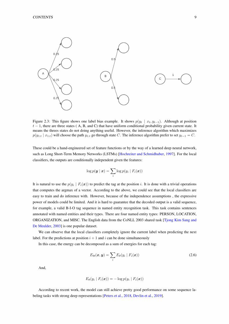
2.3 This figure shows one label bias example. It shows p(yt | xt, yt−1). Although at position
t − 1, there are three states ( A, B, and C) that have uniform conditional probability given
current state. It means the threes states do not doing anything useful. However, the inference
algorithm which maximizes p(y1:t | x1:t) will choose the path y1:t go through state C. The
inference algorithm prefer to set yt−1 = C. . . . . . . . . . . . . . . . . . . . . . . . . . 9
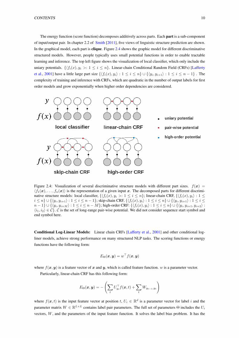
2.4 Visualization of several discriminative structure models with different part sizes. f(x) =
〈f1(x), . . . , fn(x)〉 is the representation of a given input x. The decomposed parts for
different discriminative structure models: local classifier, {〈fi(x), yi >: 1 ≤ i ≤ n};linear-chain CRF, {〈fi(x), yi〉 : 1 ≤ i ≤ n}∪{〈yi, yi+1〉 : 1 ≤ i ≤ n−1}; skip-chain CRF,
{〈fi(x), yi〉 : 1 ≤ i ≤ n}∪ {〈yi, yi+1〉 : 1 ≤ i ≤ n− 1}∪ {〈yi, yi+M 〉 : 1 ≤ i ≤ n−M};high-order CRF: {〈fi(x), yi〉 : 1 ≤ i ≤ n}∪{〈yi, yi+1, yi+2〉 : 〈i1, i2〉 ∈ C}. C is the set of
long-range pair-wise potential. We did not consider sequence start symbol and end symbol
here. . . . . . . . . . . . . . . . . . . . . . . . . . . . . . . . . . . . . . . . . . . . . . 10
2.5 A beam search example with beam size = 2. The top score hypothesis is shown in green.
The blue numbers are score(x,y) = −E(x,y). So the top score hypothesis is the hypoth-
esis with larger score in the beam. . . . . . . . . . . . . . . . . . . . . . . . . . . . . . . 21
2.6 Discrete structured output can be represented using one-hot vectors. . . . . . . . . . . . . 22
2.7 In the relaxed continuous output space, each tag output can be treat as a distribution vector
over tags. . . . . . . . . . . . . . . . . . . . . . . . . . . . . . . . . . . . . . . . . . . . 23
3.8 The architectures of inference network AΨ and energy network EΘ. . . . . . . . . . . . . 25
3.9 Discrete structured output can be represented using one-hot vectors. . . . . . . . . . . . . 25
3.10 In the relaxed continuous output space, each tag output can be treat as a distribution vector
over tags. . . . . . . . . . . . . . . . . . . . . . . . . . . . . . . . . . . . . . . . . . . . 26
3.11 Several inference network architectures. . . . . . . . . . . . . . . . . . . . . . . . . . . . 29
3.12 Development results for inference networks with different architectures and hidden sizes
(H). . . . . . . . . . . . . . . . . . . . . . . . . . . . . . . . . . . . . . . . . . . . . . . 31
3.13 Speed and accuracy comparisons of three difference inference methods: Viterbi, gradient
descent and inference network. . . . . . . . . . . . . . . . . . . . . . . . . . . . . . . . 34
3.14 Speed and search error comparisons of three difference inference methods: Viterbi, gradient
descent and inference network. . . . . . . . . . . . . . . . . . . . . . . . . . . . . . . . 36
xi
3.15 CCG test results for inference methods (GD = gradient descent). The x-axis is the total
inference time for the test set. The numbers on the GD curve are the number of gradient
descent iterations. . . . . . . . . . . . . . . . . . . . . . . . . . . . . . . . . . . . . . . 36
4.16 The performance of autogressive models and non-autoregressive models on WMT16 RO-
EN dataset. . . . . . . . . . . . . . . . . . . . . . . . . . . . . . . . . . . . . . . . . . . 39
4.17 The autogressive model can be used to score a sequence of words. The beam search algo-
rithm is also to minimize the score (Energy) . . . . . . . . . . . . . . . . . . . . . . . . . 40
4.18 The autoregressive models can be used to score a sequence of word distributions with
argmax operations. . . . . . . . . . . . . . . . . . . . . . . . . . . . . . . . . . . . . . . 40
4.19 The model for learning test-time inference networks for NAT-NMT when the energy func-
tion EΘ(x,y) is a pretrained seq2seq model with attention. . . . . . . . . . . . . . . . . 42
4.20 The architecture of CMLM. Predicting target sequence length T according to the encoder. 44
4.21 The architecture of CMLM. The decoder inputs arethe special masked tokens [M]. . . . . 44
5.22 The architectures of inference network AΨ and energy network EΘ. . . . . . . . . . . . . 50
5.23 Learned pairwise potential matrix for Twitter POS tagging. . . . . . . . . . . . . . . . . . 56
6.24 Parameterizations for cost-augmented inference network FΦ and test-time inference net-
work AΨ. . . . . . . . . . . . . . . . . . . . . . . . . . . . . . . . . . . . . . . . . . . . 62
6.25 Part-of-speech tagging training trajectories. The three curves in each setting correspond
to different random seeds. (a) Without the local CE loss, training fails when using zero
truncation. (b) The CE loss reduces the number of epochs for training. In the previous
work, we always use zero truncation and CE during training. . . . . . . . . . . . . . . . . 63
6.26 POS training trajectories with different numbers of I steps. The three curves in each setting
correspond to different random seeds. (a) cost-augmented loss after I steps; (b) margin-
rescaled hinge loss after I steps; (c) gradient norm of energy function parameters after E
steps; (d) gradient norm of test-time inference network parameters after I steps. . . . . . . 64
7.27 Visualization of the models with different orders. . . . . . . . . . . . . . . . . . . . . . . 73
7.28 Learned pairwise potential matrices W1 and W3 for NER with skip-chain energy. The rows
correspond to earlier labels and the columns correspond to subsequent labels. . . . . . . . 82
7.29 Learned 2nd-order VKP energy matrix beginning with B-PER in NER dataset. . . . . . . . 83
7.30 Visualization of the scores of 50 CNN filters on a sampled label sequence. We can observe
that filters learn the sparse set of label trigrams with strong local dependency. . . . . . . . 83
xii

Contents
1
Introduction
1.1 Structured Prediction in NLP
Structured Prediction (or Structure Prediction): In NLP applications, there exists strong complex de-
pendency between the structured outputs. We call them as structured applications here. Structured pre-
diction is a machine learning term that refers to predict the structured output in structured applications.
Such applications also appear in computer vision (e.g., image segmentation that interpreting an image of
different objects ), computational biology (e.g., protein folding that translates a protein sequence into a
three-dimensional structure). In NLP, there are lots of linguistic structure [Smith, 2011], for example,
phonology, morphology, semantic etc.
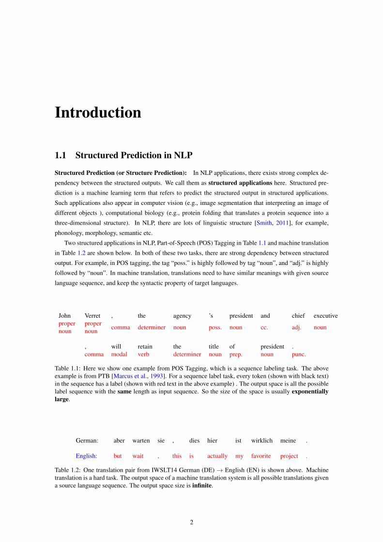
Two structured applications in NLP, Part-of-Speech (POS) Tagging in Table 1.1 and machine translation
in Table 1.2 are shown below. In both of these two tasks, there are strong dependency between structured
output. For example, in POS tagging, the tag “poss.” is highly followed by tag “noun”, and “adj.” is highly
followed by “noun”. In machine translation, translations need to have similar meanings with given source
language sequence, and keep the syntactic property of target languages.
John Verret , the agency ’s president and chief executivepropernoun
propernoun comma determiner noun poss. noun cc. adj. noun
, will retain the title of president .comma modal verb determiner noun prep. noun punc.
Table 1.1: Here we show one example from POS Tagging, which is a sequence labeling task. The aboveexample is from PTB [Marcus et al., 1993]. For a sequence label task, every token (shown with black text)in the sequence has a label (shown with red text in the above example) . The output space is all the possiblelabel sequence with the same length as input sequence. So the size of the space is usually exponentiallylarge.
German: aber warten sie , dies hier ist wirklich meine .
English: but wait , this is actually my favorite project .
Table 1.2: One translation pair from IWSLT14 German (DE) → English (EN) is shown above. Machinetranslation is a hard task. The output space of a machine translation system is all possible translations givena source language sequence. The output space size is infinite.
2
CONTENTS 3
In natural language processing, many tasks(e.g., sequence labeling, semantic role labeling, parsing, ma-
chine translation) involve predicting structured outputs. structured outputs can be a Part-of-Speech (POS)
sequence, a parser tree for parsing, an English translation, etc. There are dependencies among the labels.
It is crucial to model the dependencies between the structured output. And complex structures can ex-
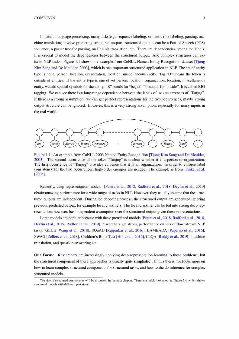
ist in NLP tasks. Figure 1.1 shows one example from CoNLL Named Entity Recognition dataset [Tjong
Kim Sang and De Meulder, 2003], which is one important structured application in NLP. The set of entity
type is none, person, location, organization, location, miscellaneous entity. Tag “O” means the token is
outside of entities. If the entity type is one of set person, location, organization, location, miscellaneous
entity, we add special symbols for the entity. “B” stands for “begin”, “I” stands for “inside”. It is called BIO
tagging. We can see there is a long-range dependence between the labels of two occurrences of “Tanjug”.
If there is a strong assumption: we can get perfect representations for the two occurrences, maybe strong
output structure can be ignored. However, this is a very strong assumption, especially for noisy inputs in
the real world.
Figure 1.1: An example from CoNLL 2003 Named Entity Recognition [Tjong Kim Sang and De Meulder,2003]. The second occurrence of the token “Tanjug” is unclear whether it is a person or organization.The first occurrence of “Tanjug” provides evidence that it is an organization. In order to enforce labelconsistency for the two occurrences, high-order energies are needed. The example is from Finkel et al.[2005].
Recently, deep representation models [Peters et al., 2018, Radford et al., 2018, Devlin et al., 2019]
obtain amazing performance for a wide range of tasks in NLP. However, they usually assume that the struc-
tured outputs are independent. During the decoding process, the structured output are generated ignoring
previous predicted output, for example local classifiers. The local classifier can be fed into strong deep rep-
resentation, however, has independent assumption over the structured output given these representations.
Large models are popular because with these pretrained models [Peters et al., 2018, Radford et al., 2018,
Devlin et al., 2019, Radford et al., 2019], researchers get strong performance on lots of downstream NLP
tasks: GLUE [Wang et al., 2018], SQuAD [Rajpurkar et al., 2016], LAMBADA [Paperno et al., 2016],
SWAG [Zellers et al., 2018], Children’s Book Test [Hill et al., 2016], CoQA [Reddy et al., 2019], machine
translation, and question answering etc.
Our Focus: Researchers are increasingly applying deep representation learning to these problems, but
the structured component of these approaches is usually quite simplistic1. In this thesis, we focus more on
how to learn complex structured components for structured tasks, and how to the do inference for complex
structured models.1The size of structured components will be discussed in the next chapter. There is a quick look about at Figure 2.4, which shows
structured models with different part sizes.
CONTENTS 4
1.2 The Benefits of Energy-Based Modeling for Structured Predic-tion
For previous structured models, the dependence of their expressivity on the structured output is limited.
Here, we present the concept of "energy-based modeling" [LeCun et al., 2006, Belanger and McCallum,
2016] to model complex dependencies between structured outputs.
Give an input sequence x and a output sequence y pair, energy-based modeling [LeCun et al., 2006,
Belanger and McCallum, 2016] associates a scalar measure E(x,y) of compatibility to each configuration
of input x and output variables y. Belanger and McCallum [2016] formulated deep energy-based models
for structured prediction, which they called structured prediction energy networks (SPENs). SPENs use
arbitrary neural networks to define the scoring function over input/output pairs. Compared with other
structured models, they are much more powerful. Energy-based models do not place any limits on the size
of the structured parts.
The potential benefits of Energy-Based modeling is to model complex structured components. For
example, sequence labeling tasks usually learn a linear-chain CRFs that only learn the weight between
successive labels and neural machine translation systems use unstructured training of local factors. For
the energy model, it could capture the arbitrary dependence, especially the long-range dependency. For
the generation, energy-based models could be used to generate outputs that favor fewer repetitions, higher
BLEU scores, or high semantic similarity with golden outputs with complex energy terms.
1.3 The Difficulties of Energy-Based Models
The energy captures dependencies between labels with flexible neural networks. However, this flexibility
of the deep energy-based models leads to challenges for learning and inference.
For inference, given the input x, we need to find a sequence y in the output space with lowest energy:
minyEΘ(x,y)
The output space is exponentially-large output space. This step is hard to jointly predict the label sequence
for a task with complex structured components because there are no strong independent assumptions. The
process can be intractable for general energy functions. Other inference problems (e.g., cost-augmented
inference and marginal inference) also require calculations over an exponentially-large output space.
The original work on SPENs used gradient descent for structured inference [Belanger and McCallum,
2016, Belanger et al., 2017]. In order to apply gradient descent for training and inference, they relax the
output space from discrete to continuous. However, it is hard to guarantee the convergence for gradient
descent inference. Furthermore, a lot of iterations could be needed for the convergence. Both of these could
slow down the inference step and decrease the performance.
In our work, we replace this use of gradient descent with a neural network trained to approximate struc-
tured inference. The neural network is called "energy-based inference network". It outputs continuous
values that we treat as the output structure.
In summary, the contributions of this thesis are as follows:
• Developing a novel inference method called "inference networks" or "energy-based inference net-
work" for structured tasks;
CONTENTS 5
• Demonstrating our proposed method achieves a better speed/accuracy/search error trade-off than gra-
dient descent, while also being faster than exact inference at similar accuracy levels;
• Applying our method on lots of structured NLP tasks, such as multi-label classification, part-of-
speech tagging, named entity recognition, semantic role labeling, and non-autoregressive machine
translation. Especially, we achieve state-of-the-art purely non-autoregressive machine translation on
the IWSLT 2014 DE-EN and WMT 2016 RO-EN datasets;
• Developing a new margin-based framework that jointly learns energy functions and inference net-
works. The proposed framework enables us to explore rich energy functions for sequence labeling
tasks.
1.4 Overview and Contributions
The thesis is organized as follows.
• In chapter 2, we summarize the history of energy-based models and some connections with previous
structured models in natural language processing. Some previous wildly used learning and inference
approaches are also discussed.
• In chapter 3, we replace this use of gradient descent with a neural network trained to approx-
imate structured argmax inference. The "inference network" outputs continuous values that we
treat as the output structure. According to our experiments, “Inference networks” achieves a bet-
ter speed/accuracy/search error trade-off than gradient descent, while also being faster than exact
inference at similar accuracy levels.
• In chapter 4, inference networks are used for non-autoregressive machine translation model training
with pretrained autoregrssive energies. We achieve state-of-the-art purely non-autoregressive results
on the IWSLT 2014 DE-EN and WMT 2016 RO-EN datasets, approaching the performance of au-
toregressive models.
• In chapter 5, we design large-margin training objectives to jointly train deep energy functions and
inference networks adversarially. As we know, it is the first that adversarial training approach is used
in structured prediction. Our training objectives resemble the alternating optimization framework of
generative adversarial networks [Goodfellow et al., 2014].
• We find that alternating optimization is a little unstable. In chapter 6, we contribute several strategies
to stabilize and improve this joint training of energy functions and inference networks for structured
prediction. We design a compound objective to jointly train both cost-augmented and test-time infer-
ence networks along with the energy function. It also simpifies our learning pipline.
• In chapter 7, we apply our framework to learn high-order models in structured applications. Neural
parameterizations of linear chain CRFs or high-order CRFs are learned with the framework proposed
in chapter 6. We empirically demonstrate that this approach achieves substantial improvement using a
variety of high-order energy terms. We also find high-order energies to help in noisy data conditions.
• Chapter 8 summarizes the contributions of the thesis and discuss some future research directions.
Our hope is that energy-based models to be applied to a larger set of natural language processing
applications, especially text generation tasks in the future.
CONTENTS 6
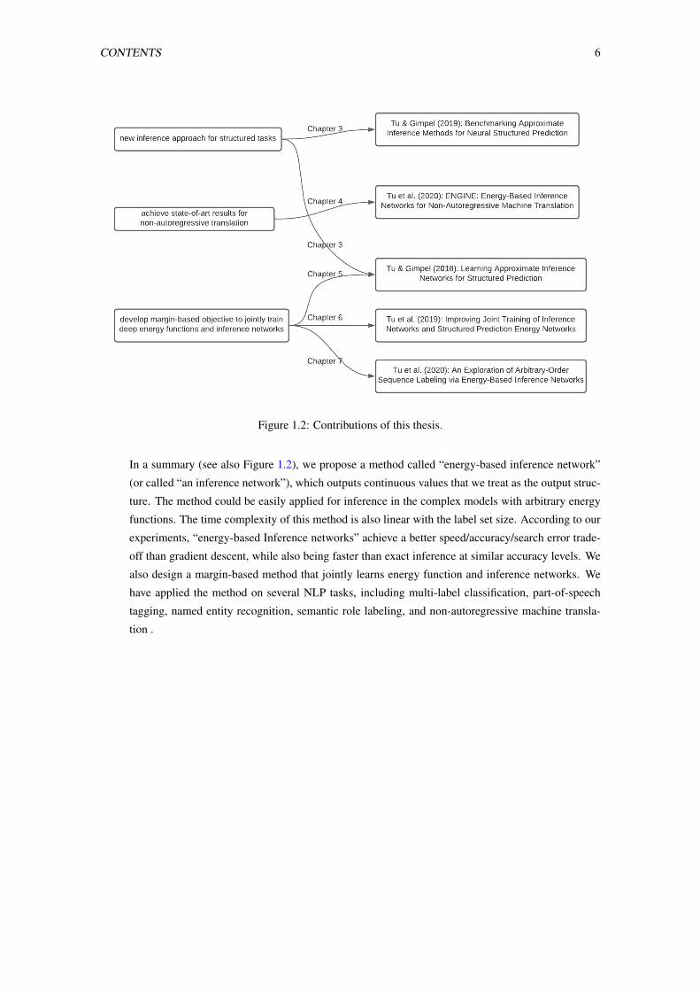
Figure 1.2: Contributions of this thesis.
In a summary (see also Figure 1.2), we propose a method called “energy-based inference network”
(or called “an inference network”), which outputs continuous values that we treat as the output struc-
ture. The method could be easily applied for inference in the complex models with arbitrary energy
functions. The time complexity of this method is also linear with the label set size. According to our
experiments, “energy-based Inference networks” achieve a better speed/accuracy/search error trade-
off than gradient descent, while also being faster than exact inference at similar accuracy levels. We
also design a margin-based method that jointly learns energy function and inference networks. We
have applied the method on several NLP tasks, including multi-label classification, part-of-speech
tagging, named entity recognition, semantic role labeling, and non-autoregressive machine transla-
tion .
Background
In this chapter, we introduce the energy-based models approach to structure prediction in NLP. The connec-
tions between energy-based models and previous approaches are discussed in particular. We then go over
some related learning and inference methods for energy-based models. We will discuss our approaches to
learning and inference for energy-based models in NLP structured applications in the following chapters.
2.1 What are Energy-Based Models
Energy-based models [Hinton, 2002, LeCun et al., 2006, Ranzato et al., 2007, Belanger and McCallum,
2016] associate a function that maps each point of a space to a scalar, which is called “energy”. The
map is called “energy function”. It is a general framework. The point of the space could be a sequence
of acoustic signals, an image, or a sequence of tokens, etc. We can treat these models as part of them:
language model [Jelinek and Mercer, 1980, Bengio et al., 2001, Peters et al., 2018, Devlin et al., 2019],
Autoencoder [Vincent et al., 2008, Vincent, 2011, Zhao et al., 2016, Xiao et al., 2021], etc.
For structured applications in NLP, the energy input space is input-output pairs X × Y . We denote
X as the set of all possible inputs, and Y as the set of all possible outputs. For a given input x ∈ X ,
we denote the space of legal structured outputs by Y(x). We denote the entire space of structured outputs
by Y = ∪x∈XY(x). Here we use Y(x) to filter ill-formed outputs [Smith, 2011]. Typically, |Y(x)| is
exponential in the size of x. The output space size is infinity in some cases (e.g., machine translation task).
The concept of an energy function Eθ used in my thesis:
EΘ : X × Y → R
is parameterized by Θ that uses a functional architecture to compute a scalar energy for an input/output
pair. The energy function can be an arbitrary function of the entire input/output pair, such as a deep neural
network.
Given an energy function, the inference step is to find the output with lowest energy:
y = argminy∈Y(x)
EΘ(x,y) (2.1)
However, solving the above search problem requires combinatorial algorithms because Y is a discrete struc-
tured space. It could become intractable when EΘ does not decompose into a sum over small “parts” of
y.
7

CONTENTS 8
2.1.1 Connection with NLP
In the NLP community, the concept “score function” is wildly used. The book by Smith [Smith, 2011],
shows that many examples of linguistic structure are considered as output to be predicted from the text.
They also demonstrate the standard approach in the NLP task is to define a score function:
score : X × Y → R (2.2)
The scoring function is generally defined as a linear model:
score(x,y) = W>F (x,y) (2.3)
Where F (x,y) is a feature extraction function and W is a weight vector.
Search-based structured prediction is formulated over possible structure:
predict(x) = argmaxy∈Y(x)
score(x,y) (2.4)
Where Y(x) is the set of all valid structures over x.
In recent years, score replace the linear scoring function over parts with a neural network.
score(x,y) =∑
part∈yNN(x, part) (2.5)
Where part is a small part in y.
We can see that the concepts of scoring function and energy function are similar. Both of them define
a function that map any point in one space to a scalar. Given an input x, the goal of learning is to make the
sample with ground truth label y have highest score.
2.1.2 Energy-Based Models for Structured Applications in NLP
In this section, we show several widely used models in NLP. Table 2.3 lists four different structured predic-
tion methods, which are widely used before.
All of them can be treated as special cases of energy-based models.
modeling learning
transition-basedP (y | x) = ΠtP (yt | x, yt−1) maxΘ
∑〈xi,yi〉∈D
logPΘ(yi | xi)
locally normalized Previous gold label is used during training.
CRFA linear model; P (y | x) is usually defined by maxΘ
∑〈xi,yi〉∈D
logPΘ(yi | xi)
uniary potential and pair-wise potential.
perceptronThe score function S is usually linear weighted minΘ
∑〈xi,yi〉∈D
[ maxy(SΘ(xi,y)−sum of the features, S(x, y) = W>f(x,y) −SΘ(xi,yi))]+
large marginThe score function S is usually linear weighted minΘ
∑〈xi,yi〉∈D
[ maxy(4(y,yi)+
sum of the features, S(x, y) = W>f(x,y) SΘ(xi,y)− SΘ(xi,yi))]+
Table 2.3: Comparisons of different structured models. D is the set of training pairs, 〈xi,yi〉 is one pairin the set, [f ]+ = max(0, f), and 4(y,y′) is a structured cost function that returns a non-negative valueindicating the difference between y and y′.
Local classifiers: This is a widely used framework. Assume we have the features for a given sequence x:
F (x) = (F1(x), F2(x), . . . , F|x|(x))
CONTENTS 9
Figure 2.3: This figure shows one label bias example. It shows p(yt | xt, yt−1). Although at positiont − 1, there are three states ( A, B, and C) that have uniform conditional probability given current state. Itmeans the threes states do not doing anything useful. However, the inference algorithm which maximizesp(y1:t | x1:t) will choose the path y1:t go through state C. The inference algorithm prefer to set yt−1 = C.
These could be a hand-engineered set of feature functions or by the way of a learned deep neural network,
such as Long Short-Term Memory Networks (LSTMs) [Hochreiter and Schmidhuber, 1997]. For the local
classifiers, the outputs are conditionally independent given the features:
log p(y | x) =∑i
log p(yi | Fi(x))
It is natural to use the p(yi | Fi(x)) to predict the tag at the position i. It is done with a trivial operations
that computes the argmax of a vector. According to the above, we could see that the local classifiers are
easy to train and do inference with. However, because of the independence assumptions , the expressive
power of models could be limited. And it is hard to guarantee that the decoded output is a valid sequence,
for example, a valid B-I-O tag sequence in named entity recognition task. This task contains sentences
annotated with named entities and their types. There are four named entity types: PERSON, LOCATION,
ORGANIZATION, and MISC. The English data from the CoNLL 2003 shared task [Tjong Kim Sang and
De Meulder, 2003] is one popular dataset.
We can observe that the local classifiers completely ignore the current label when predicting the next
label. For the predictions at position i+ 1 and i can be done simultaneously
In this case, the energy can be decomposed as a sum of energies for each tag:
EΘ(x,y) =∑i
Eθ(yi | Fi(x)) (2.6)
And,
Eθ(yi | Fi(x)) = − log p(yi | Fi(x))
According to recent work, the model can still achieve pretty good performance on some sequence la-
beling tasks with strong deep representations [Peters et al., 2018, Devlin et al., 2019].
CONTENTS 10
The energy function (score function) decomposes additively across parts. Each part is a sub-component
of input/output pair. In chapter 2.2 of Smith [2011], five views of linguistic structure prediction are shown.
In the graphical model, each part is clique. Figure 2.4 shows the graphic model for different discriminative
structured models. However, people typically uses small potential functions in order to enable tractable
learning and inference. The top left figure shows the visualization of local classifier, which only include the
uniary potentials. {〈fi(x), yi >: 1 ≤ i ≤ n}. Linear-chain Conditional Random Field (CRFs) [Lafferty
et al., 2001] have a little large part size {〈fi(x), yi〉 : 1 ≤ i ≤ n} ∪ {〈yi, yi+1〉 : 1 ≤ i ≤ n − 1} . The
complexity of training and inference with CRFs, which are quadratic in the number of output labels for first
order models and grow exponentially when higher order dependencies are considered.
Figure 2.4: Visualization of several discriminative structure models with different part sizes. f(x) =〈f1(x), . . . , fn(x)〉 is the representation of a given input x. The decomposed parts for different discrimi-native structure models: local classifier, {〈fi(x), yi >: 1 ≤ i ≤ n}; linear-chain CRF, {〈fi(x), yi〉 : 1 ≤i ≤ n} ∪ {〈yi, yi+1〉 : 1 ≤ i ≤ n− 1}; skip-chain CRF, {〈fi(x), yi〉 : 1 ≤ i ≤ n} ∪ {〈yi, yi+1〉 : 1 ≤ i ≤n− 1} ∪ {〈yi, yi+M 〉 : 1 ≤ i ≤ n−M}; high-order CRF: {〈fi(x), yi〉 : 1 ≤ i ≤ n} ∪ {〈yi, yi+1, yi+2〉 :〈i1, i2〉 ∈ C}. C is the set of long-range pair-wise potential. We did not consider sequence start symbol andend symbol here.
Conditional Log-Linear Models: Linear chain CRFs [Lafferty et al., 2001] and other conditional log-
liner models, achieve strong performance on many structured NLP tasks. The scoring functions or energy
functions have the following form:
EΘ(x,y) = w>f(x,y)
where f(x,y) is a feature vector of x and y, which is called feature function. w is a parameter vector.
Particularly, linear-chain CRF has this following form:
EΘ(x,y) = −
(∑t
U>ytf(x, t) +∑t
Wyt−1,yt
)
where f(x, t) is the input feature vector at position t, Ui ∈ Rd is a parameter vector for label i and the
parameter matrix W ∈ RL×L contains label pair parameters. The full set of parameters Θ includes the Uivectors, W , and the parameters of the input feature function. It solves the label bias problem. It has the
CONTENTS 11
efficient training and decoding based on dynamic programming for linear-chain CRF. However, it could be
computationally expensive given a large label space. And the inference could be challenging for a general
CRF framework.
Transition-Based Model: We can rewrite the conditional probability p(y | x)) as follows:
log p(y | x) =∑i
log p(yi | y1:i−1,x)
In particular, we can rewrite the above equation
EΘ(x,y) =
|y|∑t=1
et(x,y) (2.7)
where
et(x,y) = −y>t log pΘ(· | y0,y1, . . . ,yt−1,x) (2.8)
Where yt is the relaxed continuous representation of yt. In the discrete case, it is a one-hot vector. In
the continuous case, it can be probability of the tth position2. E(x,y) can be used to score a given
language pair. p(yi | y1:i−1x) can be parameterized by Recurrent Neural Networks (RNNs) or Long
Short-Term Memory Networks (LSTMs). The whole energy function Eθ(x,y) can be represented by
Sequence-to-sequence (seq2seq; Sutskever et al. 2014) models. It is common to augment models with an
attention mechanism that focuses on particular positions of the input sequence while generating the output
sequence [Bahdanau et al., 2015]. Recently, transformer-based models [Vaswani et al., 2017] are commonly
used in machine translation, summarization, question answer, or other text-based generation tasks.
The joint conditional is modeled as the product of locally normalized probability distribution over all
positions. During training, the true previous label is always used. This could cause mismatch between
training and test time, which is exposure bias [Ranzato et al., 2016]. It could also lead label bias is-
sue [Bottou, 1991]: non-generative finite-state models based on next-state classifiers (e.g., discriminative
markov models, maximum entropy Markov models [McCallum et al., 2000]), which are locally normalized,
could ignore the current observation when predicting the next label. Figure 2.3 shows one example. In the
work of [Wiseman and Rush, 2016], they use beam-search training scheme to learn global sequence scores.
General Complex Energy There has been a lot of work on using neural networks to define the potential
functions in the discriminative structure models, e.g., neural CRF [Passos et al., 2014], RNN-CRF [Huang
et al., 2015, Lample et al., 2016], CNN-CRF [Collobert et al., 2011] etc. However the potential functions
are still limited in size. Belanger and McCallum [2016] formulated deep energy-based models for struc-
tured prediction, which they called structured prediction energy networks (SPENs). SPENs use arbitraryneural networks to define the scoring function over input/output pairs. For example, they define the energy
function for multi-label classification (MLC) as the sum of two terms:
EΘ(x,y) = Eloc(x,y) + Elab(y)
2We will use the formulation in chapter 4.
CONTENTS 12
Eloc(x,y) is the sum of linear models:
Eloc(x,y) =
L∑i=1
yib>i F (x) (2.9)
where bi is a parameter vector for label i and F (x) is a multi-layer perceptron computing a feature repre-
sentation for the input x. Elab(y) scores y independent of x:
Elab(y) = c>2 g(C1y) (2.10)
where c2 is a parameter vector, g is an elementwise non-linearity function, and C1 is a parameter matrix.
Recently, structured models have been combined with deep nets [Passos et al., 2014, Huang et al., 2015,
Lample et al., 2016, Collobert et al., 2011, Hu et al., 2019, Mostajabi et al., 2018, Hwang et al., 2019,
Graber et al., 2018, Zhang et al., 2019]. However the potential functions are still limited. To address the
shortcoming, energy-based models are proposed, for instance, SPENs [Belanger and McCallum, 2016] and
GSPEN [Graber and Schwing, 2019]. They do not allow for the explicit specification of output structure.
Recently, Grathwohl et al. [2020] also demonstrate that energy based training of the joint distribution
improves calibration and robustness.
Although energy-based models have the strong ability to model complex structured components, they
have had limited application in NLP due to the computational challenges involved in learning and inference
in extremely large search spaces. In the next two subsections, we describe background on learning and
inference. It is mainly from the perspective in NLP community.
2.2 Learning of Energy-Based Models
At first, we discuss several ways for energy-based learning. There are two different approaches: probabilis-
tic and non-probabilistic learning.
2.2.1 Log loss
Probabilistic We can learn the model parameters θ, by maximizing the probability of a training set D of
data:
L =1
N
∑y∈D
log pθ(y) =1
N
∑y∈D
logexp(−Eθ(y))
Z(θ)= − logZ(θ)− 1
N
∑y∈D
Eθ(y)
N is the number of examples in training set D.
Z(θ) =
∫y
exp(−Eθ(y))
And,
p(θ) =exp(−Eθ(y))
Z(θ)
CONTENTS 13
We will derive the gradient equation by firstly writing down the partial derivative:
∂L∂θ
= −∂ logZ(θ)
∂θ− 1
N
∑y∈D
∂Eθ(y)
∂θ(2.11)
The first term compute the gradient from the partition function Z(θ), which involves an integration over y.
Then we have:
∂ logZ(θ)
∂θ=
1
Z(θ)
∂Z(θ)
∂θ
=1
Z(θ)
∂∫y
exp(−Eθ(y))
∂θ
=1
Z(θ)
∫y
∂ exp(−Eθ(y))
∂θ
=1
Z(θ)
∫y
exp(−Eθ(x))∂Eθ(y)
∂θ
=− exp(−Eθ(y))
Z(θ)
∫y
∂Eθ(y)
∂θ
=−∫y
pθ(y)∂Eθ(y)
∂θ
By putting above results into Equation 2.11:
∂L∂θ
=
∫y
pθ(y)∂Eθ(y)
∂θ− 1
N
∑y∈D
∂Eθ(y)
∂θ(2.12)
The first term could be hard and intractable. The expectation is over the model distribution.
For conditional models, we parameterize the conditional probability pθ(y | x), similarly we can get:
∂L∂θ
=∂ − log pθ(y | x)
∂θ
=∂Eθ(x,y)
∂θ−∫y′pθ(y
′ | x)∂Eθ(x,y
′)
∂θ
Typically, it is not easy to do the sampling from the model distribution. It leads in interesting research
question how to approximate the gradient. Following are several previous methods.
Contrastive Divergence: To avoid the computation difficulty of log-likelihood gradient, Hinton [2002]
uses contrastive divergence to approximate the gradient.
∂L∂θ
= Ey∈p∂Eθ(y)
∂θ− Ey∈pd
∂Eθ(y)
∂θ(2.13)
where p is the Markov Chain Monte Carlo sampling distribution from data distribution pd. In the work,
they run the chain for a small number of steps (e.g. 1). However, this technique relies on the particular form
of the energy function in the case of products of experiments, which is naturally fit to Gibbs sampling. The
intuition behind is that after a few iterations, the data moves towards the proposed distribution.
Importance Sampling: It is hard to sample from model distribution in the above equation especially if
vocabulary size is large. The idea of importance sampling is to generate k samples y1, y2, . . . , yk from an
CONTENTS 14
easy-to-sample-from distribution Q. This can be a n-gram language model. If y is a token or sequence of
tokens, The first term in Equation 2.11 can be approximate as following:
∫y
pθ(y)∂Eθ(y)
∂θ≈
k∑j=1
v(yj)
V
∂Eθ(yj)
∂θ(2.14)
where V =∑k v(yj) and v(y) = exp(−Eθ)
Q(w=y) . The normalization by V is computed with unnormalized
model distribution Eθ(y). However, the weight term v(y) = exp(−Eθ)Q(w=y) can make learn unstable because
value is with high variance. In order to reduce the variance, one way is to increase the number of samples
during training. In the work of Bengio and Senecal [2003], a few sampled negative example words are
used for language model training. A very significant speed-up is obtained.
Score Matching [Hyvärinen, 2005] and Langevin dynamics [Neal, 1993, Ranzato et al., 2007]: These
two method are not applicable when input is discrete. Both of the two method need to calculate the gra-
dient w.r.t. the random variable y. For score matching [Hyvärinen, 2005], the object bypass the intractable
unnormalized constant term Z as the following objective:
L = 0.5 ∗ Ey∈pd ||∂ log pd(y)
∂y− ∂Eθ(y)
∂y||2
where const is a constant number and pd is the data distribution.
For Langevin dynamics, it iterative update from initial sample x0 to draw sample from model distribu-
tion as following:
yt+1 = yt − 0.5 ∗ η ∗ ∂Eθ(yt)∂yt
+ ω
η is the step size and ω ∈ N (0, η) is Gaussian noise. With these samples y0,y1, . . . , the gradient from
normalization term Z is approximated.
Noise-Contrastive Estimation (NCE) [Gutmann and Hyvarinen, 2010] NCE is a more stable method
for effective training. It uses logistic regression to distinguish between the data samples from the distribution
pθ and noise samples that are generated from a noise distribution pn. If we assume the noise samples are
k times more frequent than data samples, then the posterior probability that sample w came from the data
distribution is :
P (D = 1 | w) =pd(w)
pd(w) + k ∗ pn(w)
where pd is the data distribution. We use pθ in place of pd in abve equation, then
P (D = 1 | w) =pθ(w)
pθ(w) + k ∗ pn(w)
With this posterior probability, the training objective is to maximized the following:
L = Ew∈pd logP (D = 1 | w) + k ∗ Ew∈pn logP (D = 0 | w)
CONTENTS 15
And the gradient can be expressed as:
∂L∂θ
=Ew∈pd logpd(w)
pθ(w) + k ∗ pn(w)+ k ∗ Ew∈pn log
k ∗ pn(w)
pθ(w) + k ∗ pn(w)+ k ∗ Ew∈pn
=Ew∈pdk ∗ pn(w)
pθ(w) + k ∗ pn(w)
∂ log pθ(w)
∂θ− k ∗ Ew∈pn
pθ(w)
pθ(w) + k ∗ pn(w)
∂ log pθ(w)
∂θ
=∑w
k ∗ pn(w)
pθ(w) + k ∗ pn(w)(pd − pθ)
∂ log pθ(w)
∂θ
We can see that k →∞ then:
∂L∂θ→∑w
(pd − pθ)∂ log pθ(w)
∂θ(2.15)
The gradient is 0 when the model distribution pθ match the empirical distribution pdThe good property is that the weight pd(w)
pθ(w)+k∗pn(w) are always between 0 and 1. This leads NCE
training more stable than importance sampling.
Chris’s note [Dyer, 2014] shows some analysis on NCE and negative sampling. Negative sampling
method is used in the paper [Mikolov et al., 2013]. It is similar to a special case for NCE. If there is self-
normalized assumption for the learned model distribution Pd, and the noise distribution pn = 1V and k = V .
The objective is not to optimize the likelihood of the language model. It is appropriate for representation
learning, which is not consistent with language model probabilities.
2.2.2 Margin Loss
The one wildly used objective for binary classification is the support vector machine (SVM; Cortes and
Vapnik 1995). Instead of a probabilistic view that transform score(x,y) or E(x,y) into a probability, it
takes a geometric view [Smith, 2011]. Hinge loss with multiclass setting attempts to score the correct class
above all other classes with a margin. The margin is generally set as 1. In some tasks, the margin is set as
hamming loss, L1, or L2 loss.
Ranking Loss: In some settings, there is no any supervision (with labels). However, there are a pair of
correct and incorrect one y and y′. We can use pairwise ranking approach [Cohen et al., 1998]. It is a
popular loss in NLP applications.
L(y,y′) = [4+ E(y)− E(y′)] (2.16)
In the work of Collobert et al. [2011], y is one possible text windows, y′ is the text window that the central
word of text y by another word. They use the ranking loss for learning word embeddings. In the next part,
we will talk about hinge loss used in strucutred application in NLP.
Margin-based loss: Structured Perceptron [Collins, 2002] describe an algorithm for training discrimi-
native models, for example CRF. Usually Viterbi algorithm or other algorithms are used rather than an
exhausive search in the exponentially large label space.
L =∑
〈x,y〉∈D
maxy
[E(x,y)− E(x, y)]+
CONTENTS 16
where D is the set of training pairs, [f ]+ = max(0, f). As argued in ( LeCun et al. 2006, Section 5), the
perceptron loss may not be a good loss function when training structured prediction neural networks as it
does not have a margin.
Max-margin structured learning [Tsochantaridis et al., 2004, Taskar et al., 2003] uses the following loss:
L =∑
〈x,y〉∈D
maxy
[4(y, y)− (E(x, y)− E(x,y))]+
where4 is an non-negative term, which could be a constant number. It is to measure the difference between
the candidate output y and ground-truth output y.
In the previous work, this loss is used to learning a linear modelE(x,y) = −S(x,y) = −W>f(x,y).
Recently, Belanger and McCallum [2016] use above objective to learn Structured Prediction Energy Net-
works. “cost-augmented inference step” maxy(4(y, y) − E(x, y)) is done with gradient descent based
inference. We describe gradient descent based inference in the next subsection.
There are some theory analysis and learning bounds in the work [Taskar et al., 2003, Tsochantaridis
et al., 2004]. However, in the neural-network framework, the objectives are no longer convex, and so lack
the formal guarantees and bounds associated with convex optimization problems. Similarly, the theory,
learning bounds, and guarantees associated with the algorithms do not automatically transfer to the neural
versions.
A model trained with this objective is often called a structure SVM. It enforces the model to learn good
scoring functions when incorporating cost function4.
There are also several other losses mentioned in Section 2 in the tutorial [LeCun et al., 2006].
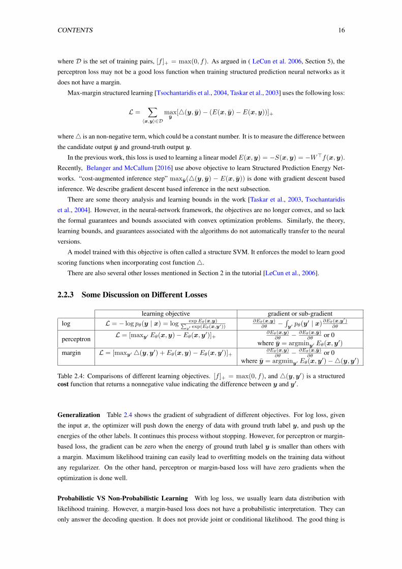
2.2.3 Some Discussion on Different Losses
learning objective gradient or sub-gradientlog L = − log pθ(y | x) = log expEθ(x,y)∑
y′ exp(Eθ(x,y′))∂Eθ(x,y)
∂θ −∫y′pθ(y
′ | x)∂Eθ(x,y′)∂θ
perceptron L = [maxy′ Eθ(x,y)− Eθ(x,y′)]+ ∂Eθ(x,y)∂θ − ∂Eθ(x,y)
∂θ or 0where y = argminy′ Eθ(x,y
′)
margin L = [maxy′ 4(y,y′) + Eθ(x,y)− Eθ(x,y′)]+ ∂Eθ(x,y)∂θ − ∂Eθ(x,y)
∂θ or 0where y = argminy′ Eθ(x,y
′)−4(y,y′)
Table 2.4: Comparisons of different learning objectives. [f ]+ = max(0, f), and 4(y,y′) is a structuredcost function that returns a nonnegative value indicating the difference between y and y′.
Generalization Table 2.4 shows the gradient of subgradient of different objectives. For log loss, given
the input x, the optimizer will push down the energy of data with ground truth label y, and push up the
energies of the other labels. It continues this process without stopping. However, for perceptron or margin-
based loss, the gradient can be zero when the energy of ground truth label y is smaller than others with
a margin. Maximum likelihood training can easily lead to overfitting models on the training data without
any regularizer. On the other hand, perceptron or margin-based loss will have zero gradients when the
optimization is done well.
Probabilistic VS Non-Probabilistic Learning With log loss, we usually learn data distribution with
likelihood training. However, a margin-based loss does not have a probabilistic interpretation. They can
only answer the decoding question. It does not provide joint or conditional likelihood. The good thing is
CONTENTS 17
that the margin-based learning use cost function 4, which is defined by the task and is related to goal or
performance metric. This provides an opportunity to learn models.
For probabilistic learning, as mentioned in ( LeCun et al. 2006, Section 1.3), it constrains∫y
exp(−E(x,y))
converges and domain Y that can be used. Hence probabilistic learning comes with a higher price. LeCun
stated that probabilistic modeling should be avoided when the application does not require it. More discus-
sions or experiments could be done in the future.
Negative Examples In the log loss, the gradient term from partition function:∫y′pθ(y
′ | x)∂Eθ(x,y
′)
∂θ
All the structured output space is considered during training. They are all “negative examples”. The com-
putation could be intractable. So approximation is done: contrastive divergence and importance sampling
are used.
In the SSVM loss, there is one step called “cost-augmented inference step”:
y = argminy′
Eθ(x,y′)−4(y,y′)
Only one negative example is used during training. However, this step could be hard and intractable.
We can see the learning signal of different objectives depend on the negative examples used.
Smith and Eisner [2005] use contrastive criterion which estimates the likelihood of the data conditioned
to a “negative neighborhood”: all sequences generated by deleting a single symbol, transposing any pair of
adjacent words, deleting any contiguous subsequence of words. Collobert et al. [2011] uses ranking loss
to learn word embedding. The negative examples are the text window that the central word of text x by
another word. So hinge loss can “inject domain knowledge“: not only the observed positive examples, but
also a set of similar but deprecated negative examples.
And “cost-augmented inference step” can be intractable and/or exact maximization has some undesir-
able quality (e.g., it’s an alternative viable prediction). In this case, maximization is replaced by sampling
Wieting et al. [2016] select the negative samples from the current minibatch.
Noise-Contrastive Estimation [Gutmann and Hyvarinen, 2010] are used for energy-based models train-
ing in some recently work [Wang and Ou, 2018b, Bakhtin et al., 2020]. The noise samples that are generated
from the noise distribution can be understood as “negative examples”. The negative examples are sampled
from pre-trained language models. Importance of negative examples also been shown in multimodel learn-
ing [Kiros et al., 2014], open-domain question answering [Karpukhin et al., 2020], model robustness [Tu
et al., 2020a] etc.
Directly Optimizing Task Metrics It is a popular approach to use maximum likelihood estimation (MLE)
for learning models. However, the performance of these models is typically evaluated with task metrics,
e.g., accuracy, F1, BLEU [Papineni et al., 2002], ROUGE [Lin, 2004]. In the previous work, reinforcement
learning (RL) objective [Ranzato et al., 2016, Norouzi et al., 2016], which is to maximize the expect reward
(task metrics) over trajectories by the policy, is used. In particular, the actor-critic approach [Barto et al.,
1983] train the actor by policy gradient with advantages of the critic. AlphaGo [Silver et al., 2016] use the
actor-critic method for self-learning in the game of Go: a value network (critic) is to evaluate positions, and
a policy network (actor) is to sample actions. However, there are still many challenges in RL for sparse
rewards.
CONTENTS 18
Gygli et al. [2017] proposes a deep value network (DVN) to estimate task metrics on different structured
outputs. In their work, the deep value network is trained on tuples comprises an input, an output, and a
corresponding oracle value (task metrics). Gradient descent3 is used for inference to iteratively find better
output, which is with lower value. It would be interesting to explore other ways of learning energy functions,
which can estimate task metrics on structured output.
2.3 Inference
In the structured applications, we need to search of y with the lowest energy over the structured output
space Y(x), which is generally exponentially large. The search space size could be even infinity if the
target sequence length is unknown. The inference problem is challenging.
argminy∈Y(x)
EΘ(x,y)
In this section, several popular inference methods in NLP are summarized here.
Greedy Decoding One simple decoding method used in the structured applications is greed decoding.
Once we know probability p(yi | .), we can do the argmax operation for position i over distribution vector.
y = argmaxyi
p(yi | .)
We can do the heuristic operations over the whole inference process for each position. It is a faster
decoding method. However, there are some constraints.
If the model is a local classifier, greed decoding is a natural choice. However, a local classifier have a
strong conditional independent assumption, which can limit model performance.
For other models, like a transition-based model, the greedy approach suffers from error propagation.
The mistakes in early decisions influence later decisions. For autoregressive models,
minyEθ(x,y) = min
y− log pθ(y | x) = min
y−∑i
log pθ(yi | y<i,x)
= miny−∑i
log pθ(yi | y<i,x)
To solve above optimization problem, one easy solution is to do argmin operation for each term y′i =
minyi − log pθ(yi | y<i,x), which is called greedy decoding. However, the greed decoding output y′ is
usually sub-optimal, because
miny−∑i
log pθ(yi | y<i,x) ≤∑i
miny′− log pθ(y
′i | y′<i,x)
Dynamic Programming Viterbi algorithm [Viterbi, 1967] is one of the popular dynamic programming
algorithms for finding the most likely sequence in NLP. In CRF or HMM, the conditional probability
3We will discuss this inference method in the next subsection.
CONTENTS 19
log p(y | x) could be decomposed similarly.
log p(y | x) =
|x|∑i=1
score1(yi, yi−1) + score2(yi,x)
here score1(yi, yi−1) is a bigram score between the label yi and yi−1, score2(yi,x) is a uniary score at
position i with label yi. Particularly, in HMM, score1(yi, yi−1) = log pη(yi | yi−1), and score2(yi,x) =
log pτ (xi | yi). The inference in HMMs or CRF is done with the following optimization:
argmaxy
|x|∑i=1
score1(yi, yi−1) + score2(yi,x) (2.17)
The above optimization problem could be solved with the dynamic programming algorithm. We set a
variable V (m, y′), which means the probability of sequence starting with label y′ at the position m. Then
we have:
V (1, y) =score1(y, 〈s〉) + score2(y,x)
V (m, y) =maxy′(score1(y, y′) + score2(y,x) + V (m− 1, y′))
〈s〉 is the start sequence symbol.The second equation could be done recursively. If we consider that the last
symbol is the end symbol 〈/s〉, then the output sequence y|x| is:
argmaxy′
score1(< /s >, y′) + V (|x|, y′)
y|x|−1, y|x|−2,..., y2, y1 are computed recursively. The time complexity is O(nL2), where n is the se-
quence length and L is the size of the label space.
For energy function has the similar form:
Eθ(x,y) =
|x|∑i=1
score1(yi, yi−1) + score2(yi,x)
Then, Viterbi algorithm can be used for decoding. However, the time complexity is O(nL2). If the label
set size L is larger, e.g., large word vocabulary size, it is not doable.
Coordinate Descent Coordinate descent algorithms [Wright, 2015] solve optimization problems by suc-
cessively performing approximate minimization along coordinate directions or coordinate hyperplanes.
When the number of coordinates is large, it is computationally expensive to solve the optimization
problem. To find the optimal solution, it makes sense to search each coordinate direction, decreasing
the objective. One potential benefit is that it is computationally cheap to search along each coordinate.
Algorithm 1 is shown below
CONTENTS 20
Algorithm 1: Coordinate Descent for finding argminy∈Y(x)EΘ(x,y)
Input: Given Energy Function:EΘ, Max Iteration Number TmaxOutput: yinitialization y(0) ;
while t < Tmax dochoose index i ∈ {1, 2, . . . , n};y
(t+1)i ← argminyi EΘ(x, yi,y
(t)−i) ;
end
y−i represent all other coordinates except i.
There are mainly two ways to choose y−i and many ways to choose the coordinate:
• Gauss-Seidel style
y(t)−i = (y
(t+1)1 , . . . , y
(t+1)i , y
(t)i+1, . . . , y
(t)n )
when updating each coordinate, the Gauss-Seidel style fixes the rest coordinates to be most up-to-date
solution. It generally converges faster.
• Jacobi style
y(t)−i = (y
(t)1 , . . . , y
(t)i , y
(t)i+1, . . . , y
(t)n )
When updating each coordinate, the Jacobi style fixes the rest coordinates to the solution from previ-
ous circle. So the Jacobi style can update coordinate in parallel for each circle.
Rules for selecting coordinates:
• Cyclic Order: choose coordinate in cyclic order, i.e. 1→ 2 · · · → n
• Randomly Sampling: randomly select coordinates
• Easy-First (Gauss−Southwell): pick coordinate i so that i = argmax1≤i≤n5Eθ(x, y1, . . . , yn)
Beam Search As mentioned in the above paragraphs, the greedy decoding approach likely does not find
the optimal solutions for autoregressive models. Algorithm 2 is shown below.
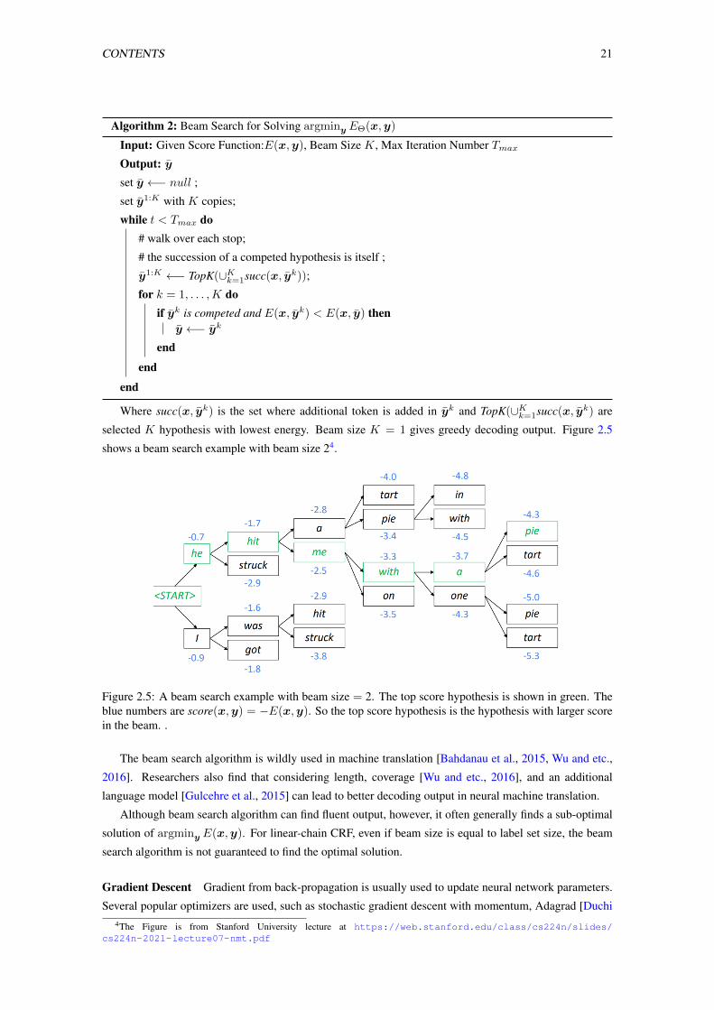
CONTENTS 21
Algorithm 2: Beam Search for Solving argminy EΘ(x,y)
Input: Given Score Function:E(x,y), Beam Size K, Max Iteration Number TmaxOutput: yset y ←− null ;
set y1:K with K copies;
while t < Tmax do# walk over each stop;
# the succession of a competed hypothesis is itself ;
y1:K ←− TopK(∪Kk=1succ(x, yk));
for k = 1, . . . ,K doif yk is competed and E(x, yk) < E(x, y) then
y ←− yk
end
end
end
Where succ(x, yk) is the set where additional token is added in yk and TopK(∪Kk=1succ(x, yk) are
selected K hypothesis with lowest energy. Beam size K = 1 gives greedy decoding output. Figure 2.5
shows a beam search example with beam size 24.
Figure 2.5: A beam search example with beam size = 2. The top score hypothesis is shown in green. Theblue numbers are score(x,y) = −E(x,y). So the top score hypothesis is the hypothesis with larger scorein the beam. .
The beam search algorithm is wildly used in machine translation [Bahdanau et al., 2015, Wu and etc.,
2016]. Researchers also find that considering length, coverage [Wu and etc., 2016], and an additional
language model [Gulcehre et al., 2015] can lead to better decoding output in neural machine translation.
Although beam search algorithm can find fluent output, however, it often generally finds a sub-optimal
solution of argminy E(x,y). For linear-chain CRF, even if beam size is equal to label set size, the beam
search algorithm is not guaranteed to find the optimal solution.
Gradient Descent Gradient from back-propagation is usually used to update neural network parameters.
Several popular optimizers are used, such as stochastic gradient descent with momentum, Adagrad [Duchi4The Figure is from Stanford University lecture at https://web.stanford.edu/class/cs224n/slides/
cs224n-2021-lecture07-nmt.pdf
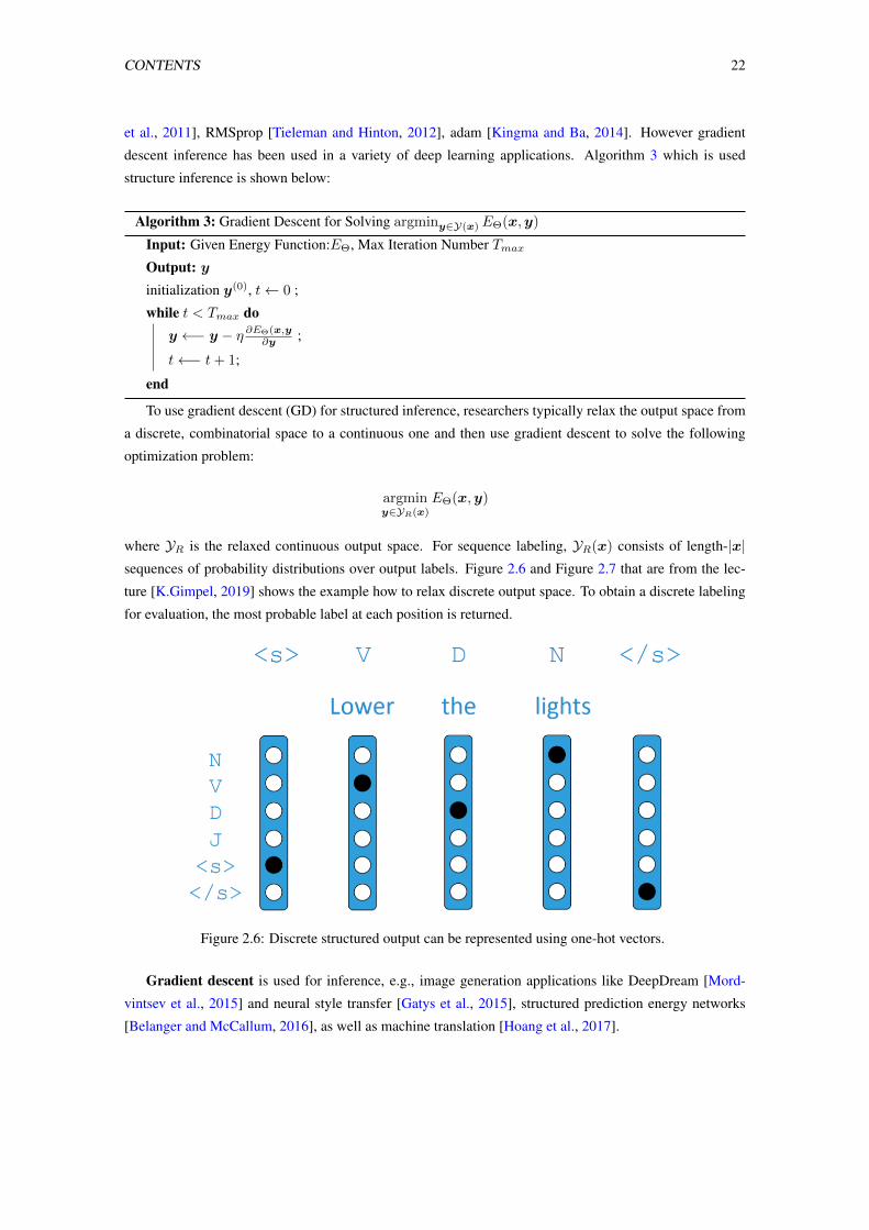
CONTENTS 22
et al., 2011], RMSprop [Tieleman and Hinton, 2012], adam [Kingma and Ba, 2014]. However gradient
descent inference has been used in a variety of deep learning applications. Algorithm 3 which is used
structure inference is shown below:
Algorithm 3: Gradient Descent for Solving argminy∈Y(x)EΘ(x,y)
Input: Given Energy Function:EΘ, Max Iteration Number TmaxOutput: yinitialization y(0), t← 0 ;
while t < Tmax doy ←− y − η ∂EΘ(x,y
∂y ;
t←− t+ 1;
end
To use gradient descent (GD) for structured inference, researchers typically relax the output space from
a discrete, combinatorial space to a continuous one and then use gradient descent to solve the following
optimization problem:
argminy∈YR(x)
EΘ(x,y)
where YR is the relaxed continuous output space. For sequence labeling, YR(x) consists of length-|x|sequences of probability distributions over output labels. Figure 2.6 and Figure 2.7 that are from the lec-
ture [K.Gimpel, 2019] shows the example how to relax discrete output space. To obtain a discrete labeling
for evaluation, the most probable label at each position is returned.
Figure 2.6: Discrete structured output can be represented using one-hot vectors.
Gradient descent is used for inference, e.g., image generation applications like DeepDream [Mord-
vintsev et al., 2015] and neural style transfer [Gatys et al., 2015], structured prediction energy networks
[Belanger and McCallum, 2016], as well as machine translation [Hoang et al., 2017].
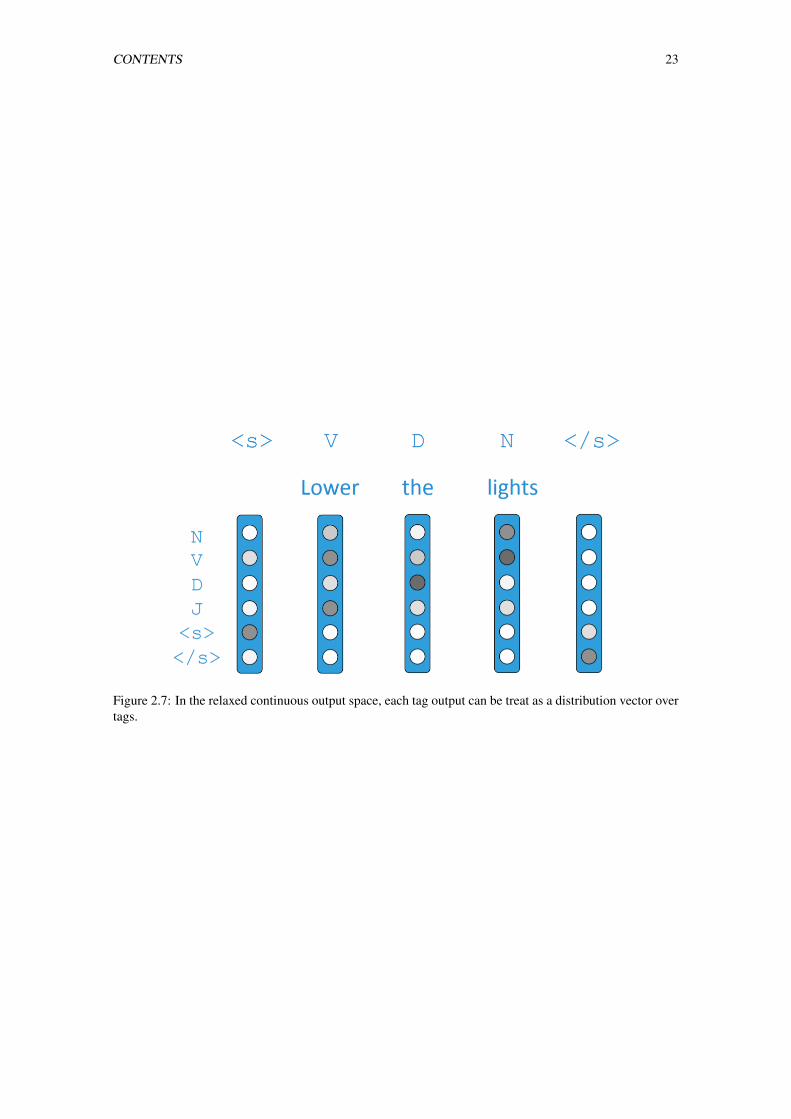
CONTENTS 23
Figure 2.7: In the relaxed continuous output space, each tag output can be treat as a distribution vector overtags.
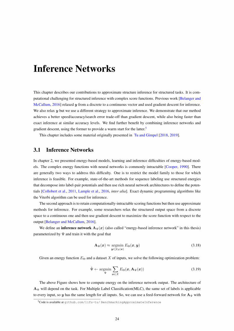
Inference Networks
This chapter describes our contributions to approximate structure inference for structured tasks. It is com-
putational challenging for structured inference with complex score functions. Previous work [Belanger and
McCallum, 2016] relaxed y from a discrete to a continuous vector and used gradient descent for inference.
We also relax y but we use a different strategy to approximate inference. We demonstrate that our method
achieves a better speed/accuracy/search error trade-off than gradient descent, while also being faster than
exact inference at similar accuracy levels. We find further benefit by combining inference networks and
gradient descent, using the former to provide a warm start for the latter.5
This chapter includes some material originally presented in Tu and Gimpel [2018, 2019].
3.1 Inference Networks
In chapter 2, we presented energy-based models, learning and inference difficulties of energy-based mod-
els. The complex energy functions with neural networks is commonly intractable [Cooper, 1990]. There
are generally two ways to address this difficulty. One is to restrict the model family to those for which
inference is feasible. For example, state-of-the-art methods for sequence labeling use structured energies
that decompose into label-pair potentials and then use rich neural network architectures to define the poten-
tials [Collobert et al., 2011, Lample et al., 2016, inter alia]. Exact dynamic programming algorithms like
the Viterbi algorithm can be used for inference.
The second approach is to retain computationally-intractable scoring functions but then use approximate
methods for inference. For example, some researchers relax the structured output space from a discrete
space to a continuous one and then use gradient descent to maximize the score function with respect to the
output [Belanger and McCallum, 2016].
We define an inference network AΨ(x) (also called “energy-based inference network” in this thesis)
parameterized by Ψ and train it with the goal that
AΨ(x) ≈ argminy∈YR(x)
EΘ(x,y) (3.18)
Given an energy function EΘ and a dataset X of inputs, we solve the following optimization problem:
Ψ← argminΨ
∑x∈X
EΘ(x,AΨ(x)) (3.19)
The above Figure shows how to compute energy on the inference network output. The architecture of
AΨ will depend on the task. For Multiple Label Classification(MLC), the same set of labels is applicable
to every input, so y has the same length for all inputs. So, we can use a feed-forward network for AΨ with
5Code is available at github.com/lifu-tu/ BenchmarkingApproximateInference
24
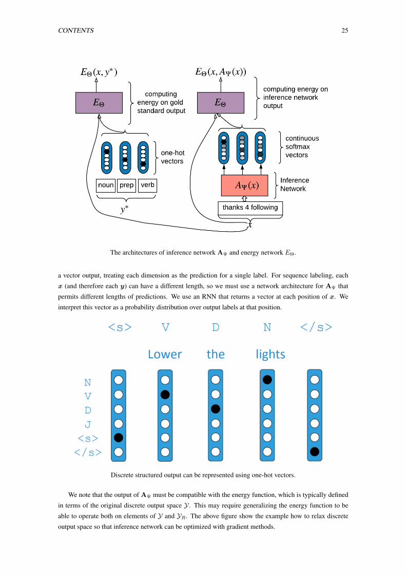
CONTENTS 25
The architectures of inference network AΨ and energy network EΘ.
a vector output, treating each dimension as the prediction for a single label. For sequence labeling, each
x (and therefore each y) can have a different length, so we must use a network architecture for AΨ that
permits different lengths of predictions. We use an RNN that returns a vector at each position of x. We
interpret this vector as a probability distribution over output labels at that position.
Discrete structured output can be represented using one-hot vectors.
We note that the output of AΨ must be compatible with the energy function, which is typically defined
in terms of the original discrete output space Y . This may require generalizing the energy function to be
able to operate both on elements of Y and YR. The above figure show the example how to relax discrete
output space so that inference network can be optimized with gradient methods.
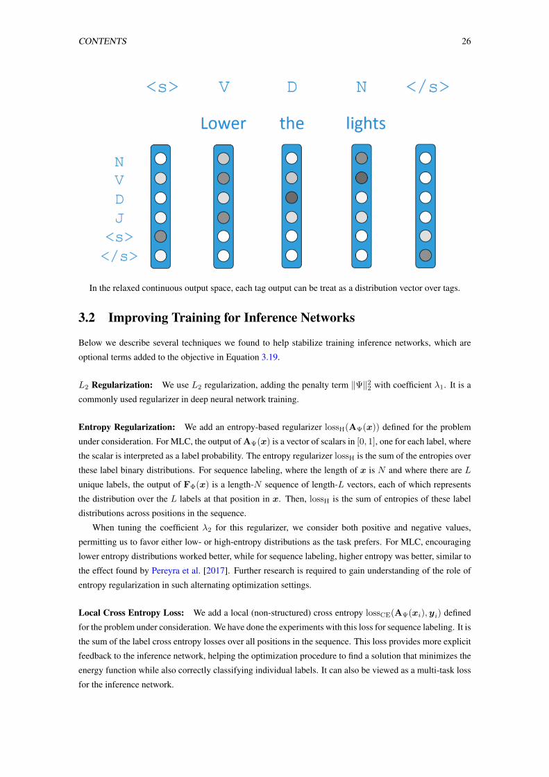
CONTENTS 26
In the relaxed continuous output space, each tag output can be treat as a distribution vector over tags.
3.2 Improving Training for Inference Networks
Below we describe several techniques we found to help stabilize training inference networks, which are
optional terms added to the objective in Equation 3.19.
L2 Regularization: We use L2 regularization, adding the penalty term ‖Ψ‖22 with coefficient λ1. It is a
commonly used regularizer in deep neural network training.
Entropy Regularization: We add an entropy-based regularizer lossH(AΨ(x)) defined for the problem
under consideration. For MLC, the output of AΨ(x) is a vector of scalars in [0, 1], one for each label, where
the scalar is interpreted as a label probability. The entropy regularizer lossH is the sum of the entropies over
these label binary distributions. For sequence labeling, where the length of x is N and where there are L
unique labels, the output of FΦ(x) is a length-N sequence of length-L vectors, each of which represents
the distribution over the L labels at that position in x. Then, lossH is the sum of entropies of these label
distributions across positions in the sequence.
When tuning the coefficient λ2 for this regularizer, we consider both positive and negative values,
permitting us to favor either low- or high-entropy distributions as the task prefers. For MLC, encouraging
lower entropy distributions worked better, while for sequence labeling, higher entropy was better, similar to
the effect found by Pereyra et al. [2017]. Further research is required to gain understanding of the role of
entropy regularization in such alternating optimization settings.
Local Cross Entropy Loss: We add a local (non-structured) cross entropy lossCE(AΨ(xi),yi) defined
for the problem under consideration. We have done the experiments with this loss for sequence labeling. It is
the sum of the label cross entropy losses over all positions in the sequence. This loss provides more explicit
feedback to the inference network, helping the optimization procedure to find a solution that minimizes the
energy function while also correctly classifying individual labels. It can also be viewed as a multi-task loss
for the inference network.
CONTENTS 27
Regularization Toward Pretrained Inference Network: We add the penalty ‖Φ− Φ0‖22 where Φ0 is a
pretrained network, e.g., a local classifier trained to independently predict each part of y.
3.3 Connections with Previous Work
Comparison to knowledge distillation: [Ba and Caruana, 2014, Hinton et al., 2015], which refers to
strategies in which one model (a “student”) is trained to mimic another (a “teacher”). Typically, the teacher
is a larger, more accurate model but which is too computationally expensive to use at test time. Urban
et al. [2016] train shallow networks using image classification data labeled by an ensemble of deep teacher
nets. Geras et al. [2016] train a convolutional network to mimic an LSTM for speech recognition. Others
have explored knowledge distillation for sequence-to-sequence learning [Kim and Rush, 2016] and pars-
ing [Kuncoro et al., 2016]. It has been empirically observed that distillation can improve generalization,
Mobahi et al. [2020] provides a theoretical analysis of distillation when the teacher and student architectures
are identical. In our methods, there is no limitation for model size of “student” and “teacher”.
Connection to amortized inference: Since we train a single inference network for an entire dataset, our
approach is also related to “amortized inference” [Srikumar et al., 2012, Gershman and Goodman, 2014,
Paige and Wood, 2016, Chang et al., 2015]. Such methods precompute or save solutions to subproblems
for faster overall computation. Our inference networks likely devote more modeling capacity to the most
frequent substructures in the data. A kind of inference network is used in variational autoencoders [Kingma
and Welling, 2013] to approximate posterior inference in generative models.
Our methods are also related to work in structured prediction that seeks to approximate structured mod-
els with factorized ones, e.g., mean-field approximations in graphical models [Koller and Friedman, 2009,
Krähenbühl and Koltun, 2011]. Like our use of inference networks, there have been efforts in designing
differentiable approximations of combinatorial search procedures [Martins and Kreutzer, 2017, Goyal et al.,
2018] and structured losses for training with them [Wiseman and Rush, 2016]. Since we relax discrete out-
put variables to be continuous, there is also a connection to recent work that focuses on structured prediction
with continuous valued output variables [Wang et al., 2016]. They also propose a formulation that yields an
alternating optimization problem, but it is based on proximal methods.
Actor-Critic: The actor-critic method is a popular reinforcement learning method, which trains a “critic”
network to provide an estimation of value given the policy of an actor network. It avoids sampling from
the policy’s (actor’s) action space, which can be expensive. The method have been applied to structure
prediction [Bahdanau et al., 2017, Zhang et al., 2017]. Comparing to the actor-critic method, In our work,
the energy function behaves as a critic network, and the inference network is similar to an actor.
Gradient descent: There are other settings in which gradient descent is used for inference, e.g., image
generation applications like DeepDream [Mordvintsev et al., 2015] and neural style transfer [Gatys et al.,
2015], as well as machine translation [Hoang et al., 2017]. In these and related settings, gradient descent has
started to be replaced by inference networks, especially for image transformation tasks [Johnson et al., 2016,
Li and Wand, 2016]. Our results below provide more evidence for making this transition. An alternative
to what we pursue here would be to obtain an easier convex optimization problem for inference via input
convex neural networks [Amos et al., 2017].
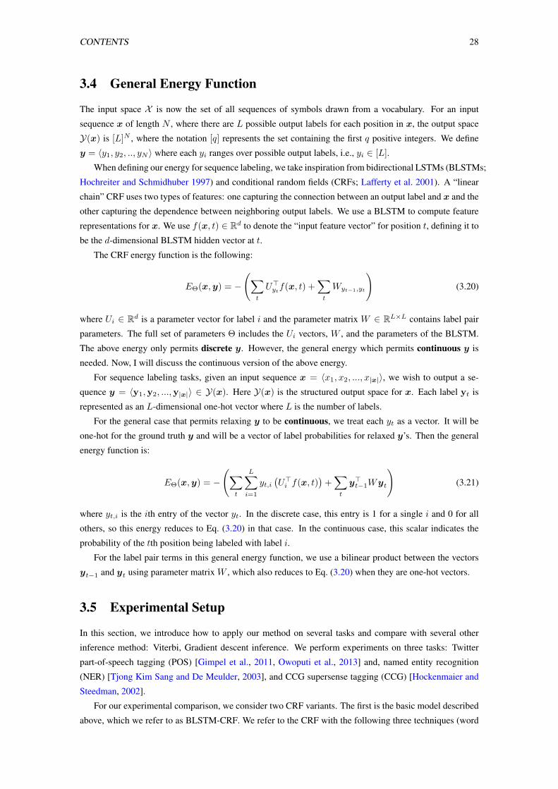
CONTENTS 28
3.4 General Energy Function
The input space X is now the set of all sequences of symbols drawn from a vocabulary. For an input
sequence x of length N , where there are L possible output labels for each position in x, the output space
Y(x) is [L]N , where the notation [q] represents the set containing the first q positive integers. We define
y = 〈y1, y2, .., yN 〉 where each yi ranges over possible output labels, i.e., yi ∈ [L].
When defining our energy for sequence labeling, we take inspiration from bidirectional LSTMs (BLSTMs;
Hochreiter and Schmidhuber 1997) and conditional random fields (CRFs; Lafferty et al. 2001). A “linear
chain” CRF uses two types of features: one capturing the connection between an output label and x and the
other capturing the dependence between neighboring output labels. We use a BLSTM to compute feature
representations for x. We use f(x, t) ∈ Rd to denote the “input feature vector” for position t, defining it to
be the d-dimensional BLSTM hidden vector at t.
The CRF energy function is the following:
EΘ(x,y) = −
(∑t
U>ytf(x, t) +∑t
Wyt−1,yt
)(3.20)
where Ui ∈ Rd is a parameter vector for label i and the parameter matrix W ∈ RL×L contains label pair
parameters. The full set of parameters Θ includes the Ui vectors, W , and the parameters of the BLSTM.
The above energy only permits discrete y. However, the general energy which permits continuous y is
needed. Now, I will discuss the continuous version of the above energy.
For sequence labeling tasks, given an input sequence x = 〈x1, x2, ..., x|x|〉, we wish to output a se-
quence y = 〈y1,y2, ...,y|x|〉 ∈ Y(x). Here Y(x) is the structured output space for x. Each label yt is
represented as an L-dimensional one-hot vector where L is the number of labels.
For the general case that permits relaxing y to be continuous, we treat each yt as a vector. It will be
one-hot for the ground truth y and will be a vector of label probabilities for relaxed y’s. Then the general
energy function is:
EΘ(x,y) = −
(∑t
L∑i=1
yt,i(U>i f(x, t)
)+∑t
y>t−1Wyt
)(3.21)
where yt,i is the ith entry of the vector yt. In the discrete case, this entry is 1 for a single i and 0 for all
others, so this energy reduces to Eq. (3.20) in that case. In the continuous case, this scalar indicates the
probability of the tth position being labeled with label i.
For the label pair terms in this general energy function, we use a bilinear product between the vectors
yt−1 and yt using parameter matrix W , which also reduces to Eq. (3.20) when they are one-hot vectors.
3.5 Experimental Setup
In this section, we introduce how to apply our method on several tasks and compare with several other
inference method: Viterbi, Gradient descent inference. We perform experiments on three tasks: Twitter
part-of-speech tagging (POS) [Gimpel et al., 2011, Owoputi et al., 2013] and, named entity recognition
(NER) [Tjong Kim Sang and De Meulder, 2003], and CCG supersense tagging (CCG) [Hockenmaier and
Steedman, 2002].
For our experimental comparison, we consider two CRF variants. The first is the basic model described
above, which we refer to as BLSTM-CRF. We refer to the CRF with the following three techniques (word
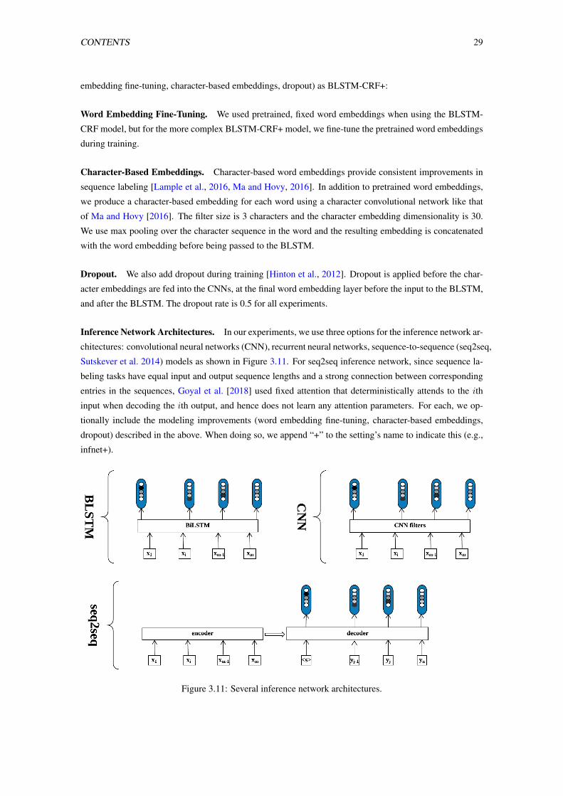
CONTENTS 29
embedding fine-tuning, character-based embeddings, dropout) as BLSTM-CRF+:
Word Embedding Fine-Tuning. We used pretrained, fixed word embeddings when using the BLSTM-
CRF model, but for the more complex BLSTM-CRF+ model, we fine-tune the pretrained word embeddings
during training.
Character-Based Embeddings. Character-based word embeddings provide consistent improvements in
sequence labeling [Lample et al., 2016, Ma and Hovy, 2016]. In addition to pretrained word embeddings,
we produce a character-based embedding for each word using a character convolutional network like that
of Ma and Hovy [2016]. The filter size is 3 characters and the character embedding dimensionality is 30.
We use max pooling over the character sequence in the word and the resulting embedding is concatenated
with the word embedding before being passed to the BLSTM.
Dropout. We also add dropout during training [Hinton et al., 2012]. Dropout is applied before the char-
acter embeddings are fed into the CNNs, at the final word embedding layer before the input to the BLSTM,
and after the BLSTM. The dropout rate is 0.5 for all experiments.
Inference Network Architectures. In our experiments, we use three options for the inference network ar-
chitectures: convolutional neural networks (CNN), recurrent neural networks, sequence-to-sequence (seq2seq,
Sutskever et al. 2014) models as shown in Figure 3.11. For seq2seq inference network, since sequence la-
beling tasks have equal input and output sequence lengths and a strong connection between corresponding
entries in the sequences, Goyal et al. [2018] used fixed attention that deterministically attends to the ith
input when decoding the ith output, and hence does not learn any attention parameters. For each, we op-
tionally include the modeling improvements (word embedding fine-tuning, character-based embeddings,
dropout) described in the above. When doing so, we append “+” to the setting’s name to indicate this (e.g.,
infnet+).
Figure 3.11: Several inference network architectures.
CONTENTS 30
Gradient Descent for Inference Details To use gradient descent (GD) for structured inference, we need
to solve the following optimization problem:
argminy∈YR(x)
EΘ(x,y)
where YR is the relaxed continuous output space. For sequence labeling, YR(x) consists of length-|x|sequences of probability distributions over output labels. To obtain a discrete labeling for evaluation, the
most probable label at each position is returned.
Gradient descent has the advantage of simplicity. Standard autodifferentiation toolkits can be used to
compute gradients of the energy with respect to the output once the output space has been relaxed. However,
one challenge is maintaining constraints on the variables being optimized.
Therefore, we actually perform gradient descent in an relaxed output space YR′(x) which consists of
length-|x| sequences of vectors, where each vector yt ∈ RL. When computing the energy, we use a softmax
transformation on each yt, solving the following optimization problem with gradient descent:
argminy∈YR′ (x)
EΘ(x, softmax(y)) (3.22)
where the softmax operation above is applied independently to each vector yt in the output structure y.
For the number of epochs N , we consider values in the set {5, 10, 20, 30, 40, 50, 100, 500, 1000}. For
each N , we tune the learning rate over the set {1e4, 5e3, 1e3, 500, 100, 50, 10, 5, 1}). These learning rates
may appear extremely large when we are accustomed to choosing rates for empirical risk minimization, but
we generally found that the most effective learning rates for structured inference are orders of magnitude
larger than those effective for learning. To provide as strong performance as possible for the gradient
descent method, we tune N and the learning rate via oracle tuning, i.e., we choose them separately for each
input to maximize performance (accuracy or F1 score) on that input.
3.6 Training Objective
For training the inference network parameters Ψ, we find that a local cross entropy loss consistently worked
well for sequence labeling. We use this local cross entropy loss in this proposal, so we perform learning by
solving the following:
argminΨ
∑〈x,y〉
EΘ(x,AΨ(x))+λ`token(y,AΨ(x))
where the sum is over 〈x,y〉 pairs in the training set. The token-level loss is defined:
`token(y,A(x)) =
|y|∑t=1
CE(yt,A(x)t) (3.23)
where yt is the L-dimensional one-hot label vector at position t in y, A(x)t is the inference network’s
output distribution at position t, and CE stands for cross entropy. `token is the loss used in our non-
structured baseline models.
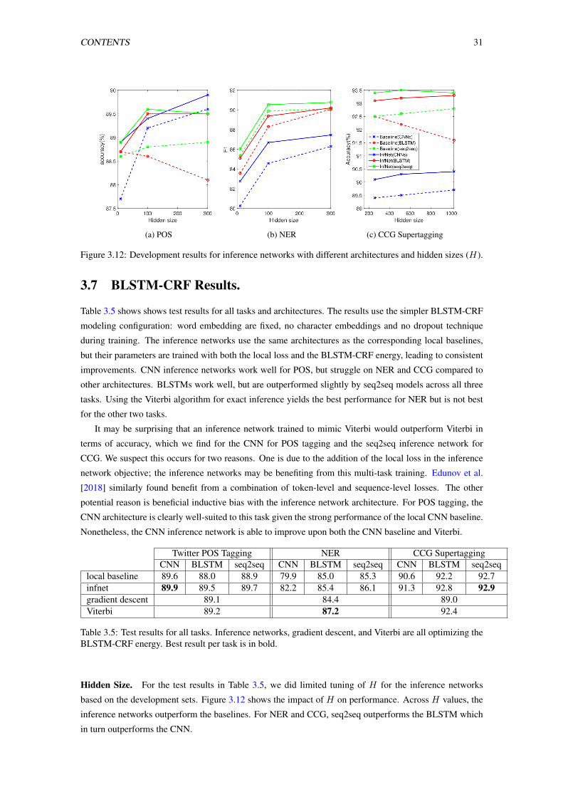
CONTENTS 31
(a) POS (b) NER (c) CCG Supertagging
Figure 3.12: Development results for inference networks with different architectures and hidden sizes (H).
3.7 BLSTM-CRF Results.
Table 3.5 shows shows test results for all tasks and architectures. The results use the simpler BLSTM-CRF
modeling configuration: word embedding are fixed, no character embeddings and no dropout technique
during training. The inference networks use the same architectures as the corresponding local baselines,
but their parameters are trained with both the local loss and the BLSTM-CRF energy, leading to consistent
improvements. CNN inference networks work well for POS, but struggle on NER and CCG compared to
other architectures. BLSTMs work well, but are outperformed slightly by seq2seq models across all three
tasks. Using the Viterbi algorithm for exact inference yields the best performance for NER but is not best
for the other two tasks.
It may be surprising that an inference network trained to mimic Viterbi would outperform Viterbi in
terms of accuracy, which we find for the CNN for POS tagging and the seq2seq inference network for
CCG. We suspect this occurs for two reasons. One is due to the addition of the local loss in the inference
network objective; the inference networks may be benefiting from this multi-task training. Edunov et al.
[2018] similarly found benefit from a combination of token-level and sequence-level losses. The other
potential reason is beneficial inductive bias with the inference network architecture. For POS tagging, the
CNN architecture is clearly well-suited to this task given the strong performance of the local CNN baseline.
Nonetheless, the CNN inference network is able to improve upon both the CNN baseline and Viterbi.
Twitter POS Tagging NER CCG SupertaggingCNN BLSTM seq2seq CNN BLSTM seq2seq CNN BLSTM seq2seq
local baseline 89.6 88.0 88.9 79.9 85.0 85.3 90.6 92.2 92.7infnet 89.9 89.5 89.7 82.2 85.4 86.1 91.3 92.8 92.9gradient descent 89.1 84.4 89.0Viterbi 89.2 87.2 92.4
Table 3.5: Test results for all tasks. Inference networks, gradient descent, and Viterbi are all optimizing theBLSTM-CRF energy. Best result per task is in bold.
Hidden Size. For the test results in Table 3.5, we did limited tuning of H for the inference networks
based on the development sets. Figure 3.12 shows the impact of H on performance. Across H values, the
inference networks outperform the baselines. For NER and CCG, seq2seq outperforms the BLSTM which
in turn outperforms the CNN.
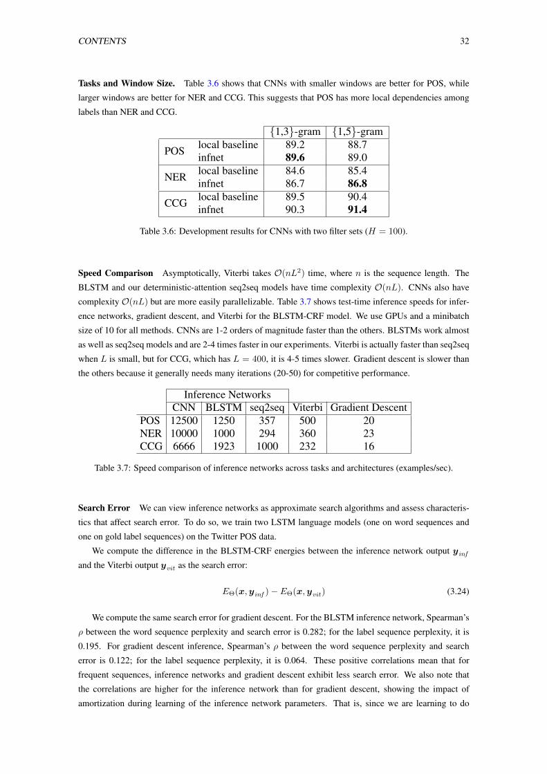
CONTENTS 32
Tasks and Window Size. Table 3.6 shows that CNNs with smaller windows are better for POS, while
larger windows are better for NER and CCG. This suggests that POS has more local dependencies among
labels than NER and CCG.
{1,3}-gram {1,5}-gram
POS local baseline 89.2 88.7infnet 89.6 89.0
NER local baseline 84.6 85.4infnet 86.7 86.8
CCG local baseline 89.5 90.4infnet 90.3 91.4
Table 3.6: Development results for CNNs with two filter sets (H = 100).
Speed Comparison Asymptotically, Viterbi takes O(nL2) time, where n is the sequence length. The
BLSTM and our deterministic-attention seq2seq models have time complexity O(nL). CNNs also have
complexity O(nL) but are more easily parallelizable. Table 3.7 shows test-time inference speeds for infer-
ence networks, gradient descent, and Viterbi for the BLSTM-CRF model. We use GPUs and a minibatch
size of 10 for all methods. CNNs are 1-2 orders of magnitude faster than the others. BLSTMs work almost
as well as seq2seq models and are 2-4 times faster in our experiments. Viterbi is actually faster than seq2seq
when L is small, but for CCG, which has L = 400, it is 4-5 times slower. Gradient descent is slower than
the others because it generally needs many iterations (20-50) for competitive performance.
Inference NetworksCNN BLSTM seq2seq Viterbi Gradient Descent
POS 12500 1250 357 500 20NER 10000 1000 294 360 23CCG 6666 1923 1000 232 16
Table 3.7: Speed comparison of inference networks across tasks and architectures (examples/sec).
Search Error We can view inference networks as approximate search algorithms and assess characteris-
tics that affect search error. To do so, we train two LSTM language models (one on word sequences and
one on gold label sequences) on the Twitter POS data.
We compute the difference in the BLSTM-CRF energies between the inference network output yinf
and the Viterbi output yvit as the search error:
EΘ(x,yinf )− EΘ(x,yvit) (3.24)
We compute the same search error for gradient descent. For the BLSTM inference network, Spearman’s
ρ between the word sequence perplexity and search error is 0.282; for the label sequence perplexity, it is
0.195. For gradient descent inference, Spearman’s ρ between the word sequence perplexity and search
error is 0.122; for the label sequence perplexity, it is 0.064. These positive correlations mean that for
frequent sequences, inference networks and gradient descent exhibit less search error. We also note that
the correlations are higher for the inference network than for gradient descent, showing the impact of
amortization during learning of the inference network parameters. That is, since we are learning to do
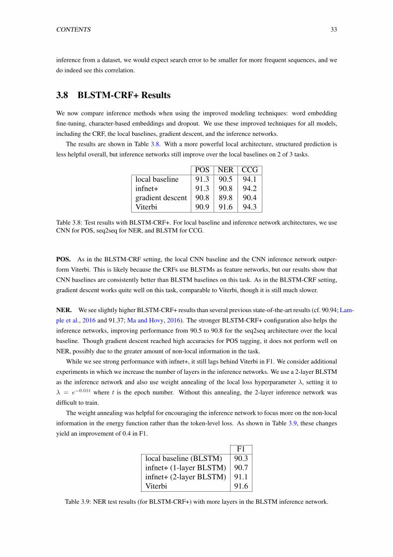
CONTENTS 33
inference from a dataset, we would expect search error to be smaller for more frequent sequences, and we
do indeed see this correlation.
3.8 BLSTM-CRF+ Results
We now compare inference methods when using the improved modeling techniques: word embedding
fine-tuning, character-based embeddings and dropout. We use these improved techniques for all models,
including the CRF, the local baselines, gradient descent, and the inference networks.
The results are shown in Table 3.8. With a more powerful local architecture, structured prediction is
less helpful overall, but inference networks still improve over the local baselines on 2 of 3 tasks.
POS NER CCGlocal baseline 91.3 90.5 94.1infnet+ 91.3 90.8 94.2gradient descent 90.8 89.8 90.4Viterbi 90.9 91.6 94.3
Table 3.8: Test results with BLSTM-CRF+. For local baseline and inference network architectures, we useCNN for POS, seq2seq for NER, and BLSTM for CCG.
POS. As in the BLSTM-CRF setting, the local CNN baseline and the CNN inference network outper-
form Viterbi. This is likely because the CRFs use BLSTMs as feature networks, but our results show that
CNN baselines are consistently better than BLSTM baselines on this task. As in the BLSTM-CRF setting,
gradient descent works quite well on this task, comparable to Viterbi, though it is still much slower.
NER. We see slightly higher BLSTM-CRF+ results than several previous state-of-the-art results (cf. 90.94; Lam-
ple et al., 2016 and 91.37; Ma and Hovy, 2016). The stronger BLSTM-CRF+ configuration also helps the
inference networks, improving performance from 90.5 to 90.8 for the seq2seq architecture over the local
baseline. Though gradient descent reached high accuracies for POS tagging, it does not perform well on
NER, possibly due to the greater amount of non-local information in the task.
While we see strong performance with infnet+, it still lags behind Viterbi in F1. We consider additional
experiments in which we increase the number of layers in the inference networks. We use a 2-layer BLSTM
as the inference network and also use weight annealing of the local loss hyperparameter λ, setting it to
λ = e−0.01t where t is the epoch number. Without this annealing, the 2-layer inference network was
difficult to train.
The weight annealing was helpful for encouraging the inference network to focus more on the non-local
information in the energy function rather than the token-level loss. As shown in Table 3.9, these changes
yield an improvement of 0.4 in F1.
F1local baseline (BLSTM) 90.3infnet+ (1-layer BLSTM) 90.7infnet+ (2-layer BLSTM) 91.1Viterbi 91.6
Table 3.9: NER test results (for BLSTM-CRF+) with more layers in the BLSTM inference network.
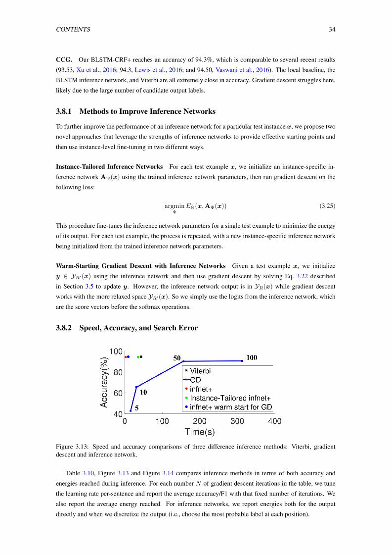
CONTENTS 34
CCG. Our BLSTM-CRF+ reaches an accuracy of 94.3%, which is comparable to several recent results
(93.53, Xu et al., 2016; 94.3, Lewis et al., 2016; and 94.50, Vaswani et al., 2016). The local baseline, the
BLSTM inference network, and Viterbi are all extremely close in accuracy. Gradient descent struggles here,
likely due to the large number of candidate output labels.
3.8.1 Methods to Improve Inference Networks
To further improve the performance of an inference network for a particular test instance x, we propose two
novel approaches that leverage the strengths of inference networks to provide effective starting points and
then use instance-level fine-tuning in two different ways.
Instance-Tailored Inference Networks For each test example x, we initialize an instance-specific in-
ference network AΨ(x) using the trained inference network parameters, then run gradient descent on the
following loss:
argminΨ
EΘ(x,AΨ(x)) (3.25)
This procedure fine-tunes the inference network parameters for a single test example to minimize the energy
of its output. For each test example, the process is repeated, with a new instance-specific inference network
being initialized from the trained inference network parameters.
Warm-Starting Gradient Descent with Inference Networks Given a test example x, we initialize
y ∈ YR′(x) using the inference network and then use gradient descent by solving Eq. 3.22 described
in Section 3.5 to update y. However, the inference network output is in YR(x) while gradient descent
works with the more relaxed space YR′(x). So we simply use the logits from the inference network, which
are the score vectors before the softmax operations.
3.8.2 Speed, Accuracy, and Search Error
Figure 3.13: Speed and accuracy comparisons of three difference inference methods: Viterbi, gradientdescent and inference network.
Table 3.10, Figure 3.13 and Figure 3.14 compares inference methods in terms of both accuracy and
energies reached during inference. For each number N of gradient descent iterations in the table, we tune
the learning rate per-sentence and report the average accuracy/F1 with that fixed number of iterations. We
also report the average energy reached. For inference networks, we report energies both for the output
directly and when we discretize the output (i.e., choose the most probable label at each position).
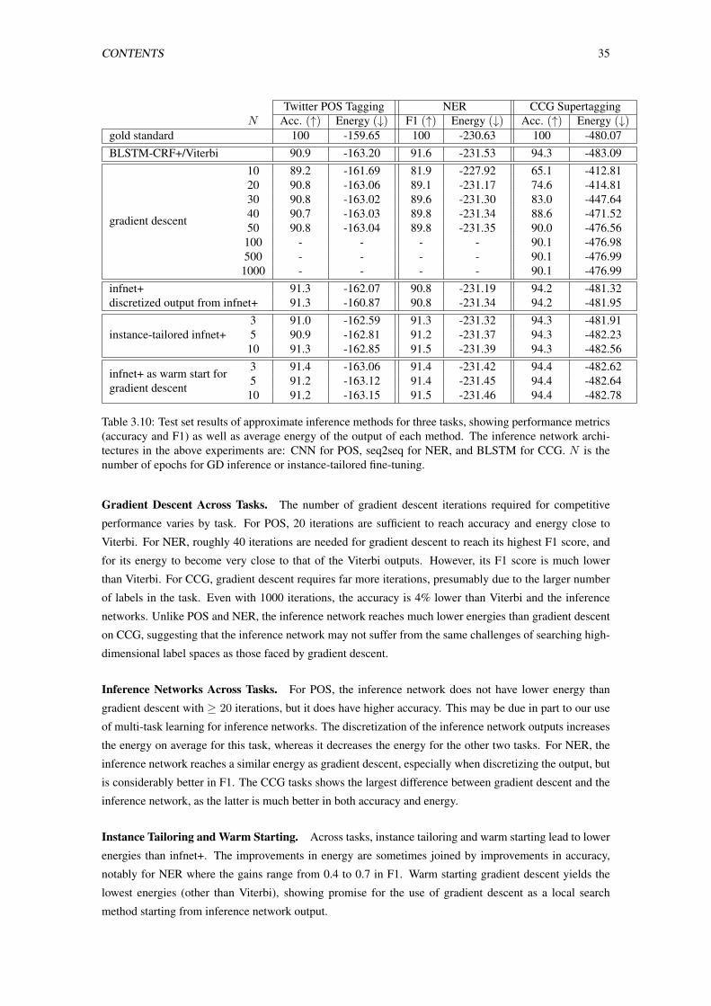
CONTENTS 35
Twitter POS Tagging NER CCG SupertaggingN Acc. (↑) Energy (↓) F1 (↑) Energy (↓) Acc. (↑) Energy (↓)
gold standard 100 -159.65 100 -230.63 100 -480.07BLSTM-CRF+/Viterbi 90.9 -163.20 91.6 -231.53 94.3 -483.09
10 89.2 -161.69 81.9 -227.92 65.1 -412.8120 90.8 -163.06 89.1 -231.17 74.6 -414.8130 90.8 -163.02 89.6 -231.30 83.0 -447.64
gradient descent 40 90.7 -163.03 89.8 -231.34 88.6 -471.5250 90.8 -163.04 89.8 -231.35 90.0 -476.56100 - - - - 90.1 -476.98500 - - - - 90.1 -476.99
1000 - - - - 90.1 -476.99infnet+ 91.3 -162.07 90.8 -231.19 94.2 -481.32discretized output from infnet+ 91.3 -160.87 90.8 -231.34 94.2 -481.95
3 91.0 -162.59 91.3 -231.32 94.3 -481.91instance-tailored infnet+ 5 90.9 -162.81 91.2 -231.37 94.3 -482.23
10 91.3 -162.85 91.5 -231.39 94.3 -482.56
infnet+ as warm start for 3 91.4 -163.06 91.4 -231.42 94.4 -482.62
gradient descent 5 91.2 -163.12 91.4 -231.45 94.4 -482.6410 91.2 -163.15 91.5 -231.46 94.4 -482.78
Table 3.10: Test set results of approximate inference methods for three tasks, showing performance metrics(accuracy and F1) as well as average energy of the output of each method. The inference network archi-tectures in the above experiments are: CNN for POS, seq2seq for NER, and BLSTM for CCG. N is thenumber of epochs for GD inference or instance-tailored fine-tuning.
Gradient Descent Across Tasks. The number of gradient descent iterations required for competitive
performance varies by task. For POS, 20 iterations are sufficient to reach accuracy and energy close to
Viterbi. For NER, roughly 40 iterations are needed for gradient descent to reach its highest F1 score, and
for its energy to become very close to that of the Viterbi outputs. However, its F1 score is much lower
than Viterbi. For CCG, gradient descent requires far more iterations, presumably due to the larger number
of labels in the task. Even with 1000 iterations, the accuracy is 4% lower than Viterbi and the inference
networks. Unlike POS and NER, the inference network reaches much lower energies than gradient descent
on CCG, suggesting that the inference network may not suffer from the same challenges of searching high-
dimensional label spaces as those faced by gradient descent.
Inference Networks Across Tasks. For POS, the inference network does not have lower energy than
gradient descent with ≥ 20 iterations, but it does have higher accuracy. This may be due in part to our use
of multi-task learning for inference networks. The discretization of the inference network outputs increases
the energy on average for this task, whereas it decreases the energy for the other two tasks. For NER, the
inference network reaches a similar energy as gradient descent, especially when discretizing the output, but
is considerably better in F1. The CCG tasks shows the largest difference between gradient descent and the
inference network, as the latter is much better in both accuracy and energy.
Instance Tailoring and Warm Starting. Across tasks, instance tailoring and warm starting lead to lower
energies than infnet+. The improvements in energy are sometimes joined by improvements in accuracy,
notably for NER where the gains range from 0.4 to 0.7 in F1. Warm starting gradient descent yields the
lowest energies (other than Viterbi), showing promise for the use of gradient descent as a local search
method starting from inference network output.
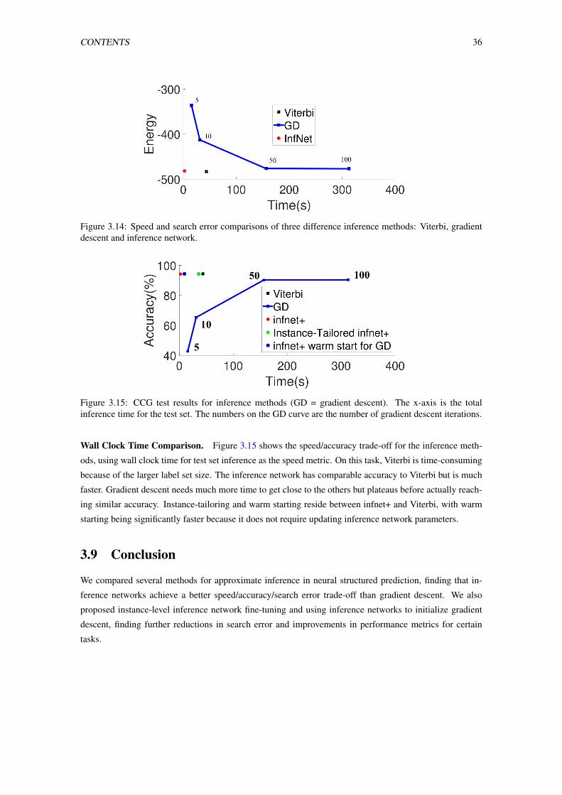
CONTENTS 36
Figure 3.14: Speed and search error comparisons of three difference inference methods: Viterbi, gradientdescent and inference network.
Figure 3.15: CCG test results for inference methods (GD = gradient descent). The x-axis is the totalinference time for the test set. The numbers on the GD curve are the number of gradient descent iterations.
Wall Clock Time Comparison. Figure 3.15 shows the speed/accuracy trade-off for the inference meth-
ods, using wall clock time for test set inference as the speed metric. On this task, Viterbi is time-consuming
because of the larger label set size. The inference network has comparable accuracy to Viterbi but is much
faster. Gradient descent needs much more time to get close to the others but plateaus before actually reach-
ing similar accuracy. Instance-tailoring and warm starting reside between infnet+ and Viterbi, with warm
starting being significantly faster because it does not require updating inference network parameters.
3.9 Conclusion
We compared several methods for approximate inference in neural structured prediction, finding that in-
ference networks achieve a better speed/accuracy/search error trade-off than gradient descent. We also
proposed instance-level inference network fine-tuning and using inference networks to initialize gradient
descent, finding further reductions in search error and improvements in performance metrics for certain
tasks.
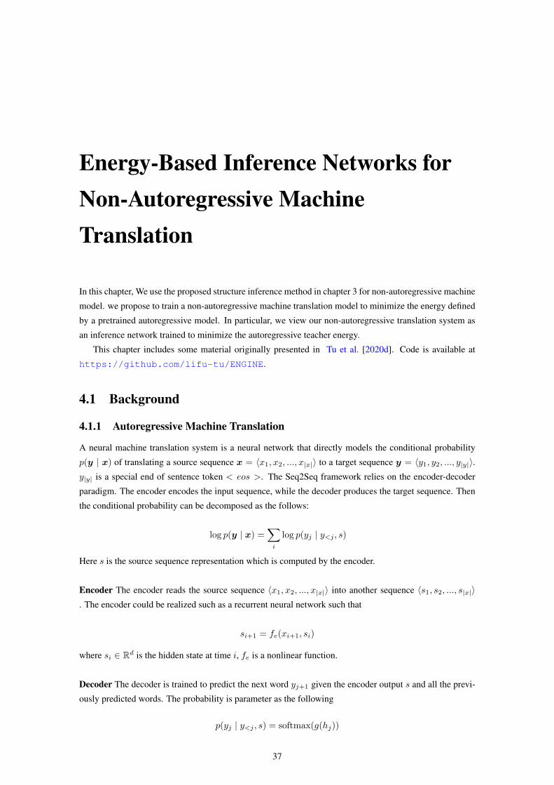
Energy-Based Inference Networks forNon-Autoregressive MachineTranslation
In this chapter, We use the proposed structure inference method in chapter 3 for non-autoregressive machine
model. we propose to train a non-autoregressive machine translation model to minimize the energy defined
by a pretrained autoregressive model. In particular, we view our non-autoregressive translation system as
an inference network trained to minimize the autoregressive teacher energy.
This chapter includes some material originally presented in Tu et al. [2020d]. Code is available at
https://github.com/lifu-tu/ENGINE.
4.1 Background
4.1.1 Autoregressive Machine Translation
A neural machine translation system is a neural network that directly models the conditional probability
p(y | x) of translating a source sequence x = 〈x1, x2, ..., x|x|〉 to a target sequence y = 〈y1, y2, ..., y|y|〉.y|y| is a special end of sentence token < eos >. The Seq2Seq framework relies on the encoder-decoder
paradigm. The encoder encodes the input sequence, while the decoder produces the target sequence. Then
the conditional probability can be decomposed as the follows:
log p(y | x) =∑i
log p(yj | y<j , s)
Here s is the source sequence representation which is computed by the encoder.
Encoder The encoder reads the source sequence 〈x1, x2, ..., x|x|〉 into another sequence 〈s1, s2, ..., s|x|〉. The encoder could be realized such as a recurrent neural network such that
si+1 = fe(xi+1, si)
where si ∈ Rd is the hidden state at time i, fe is a nonlinear function.
Decoder The decoder is trained to predict the next word yj+1 given the encoder output s and all the previ-
ously predicted words. The probability is parameter as the following
p(yj | y<j , s) = softmax(g(hj))
37
CONTENTS 38
with g is a transformation function that outputs a vocabulary-sized vector. Here hj is also the RNN hidden
unit of the decoder at time step j, which is could computed as:
hj = fd(hj−1, yj−1) (4.26)
Here fd is also a nonlinear function.
For the attention-based models, the attention hidden state h is difference from the above. It is computed as
follows:
hj = f(Wc[hj , cj ])
Here cj is the source-side context vector.
p(yj | y<j , s) = softmax(Wdhj)
The aligned vector at, whose size is equal the number of time step on the source sentence.
aj(i) =exp(score(hj , si))∑i′ exp(score(hj , si′))
There are three different alternatives to compute the score. In my experiment, I just use the following
general one:
score(hj , si) = hTj Wasi
The context vector cj is then computed as the weighted sum of the source hidden vector hi as follow:
cj =
|x|∑i=1
aj(i)si
The computation graph is simple, we can go from hj → aj(i)→ cj → hj → yj , which follow Luong
et al. [2015] ’s step. Bahdanau et al. [2015] at each time j, go from hj−1 → aj(i)→ cj → hj → yj .
4.1.2 Non-autoregresive Machine Translation System
In the work [Gu et al., 2018], they introduce non-autoregressive neural machine translation (NAT) systems
based on transformer network [Vaswani et al., 2017] in order to remove the autoregressive connection and
do parallel decoding. The naive solution is to have the following assumption:
log pθ(y | x) =
|y|∑t=1
log pθ(yt | x)
The target token is independent given the input. Unfortunately, the performance of non-autoregressive
models fall far behind autoregressive models.
The performance of non-autoregressive neural machine translation (NAT) systems, which predict tokens
in the target language independently of each other conditioned on the source sentence, has been improving
steadily in recent years [Lee et al., 2018, Ghazvininejad et al., 2019, Ma et al., 2019]. The performance
of several non-autoregressive modes are shown in Figure 4.16. One common ingredient in getting non-
autoregressive systems to perform well is to train them on a corpus of distilled translations [Kim and Rush,
2016]. This distilled corpus consists of source sentences paired with the translations produced by a pre-
trained autoregressive “teacher” system.
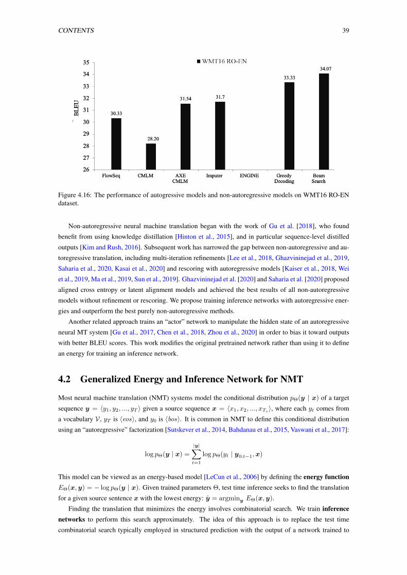
CONTENTS 39
Figure 4.16: The performance of autogressive models and non-autoregressive models on WMT16 RO-ENdataset.
Non-autoregressive neural machine translation began with the work of Gu et al. [2018], who found
benefit from using knowledge distillation [Hinton et al., 2015], and in particular sequence-level distilled
outputs [Kim and Rush, 2016]. Subsequent work has narrowed the gap between non-autoregressive and au-
toregressive translation, including multi-iteration refinements [Lee et al., 2018, Ghazvininejad et al., 2019,
Saharia et al., 2020, Kasai et al., 2020] and rescoring with autoregressive models [Kaiser et al., 2018, Wei
et al., 2019, Ma et al., 2019, Sun et al., 2019]. Ghazvininejad et al. [2020] and Saharia et al. [2020] proposed
aligned cross entropy or latent alignment models and achieved the best results of all non-autoregressive
models without refinement or rescoring. We propose training inference networks with autoregressive ener-
gies and outperform the best purely non-autoregressive methods.
Another related approach trains an “actor” network to manipulate the hidden state of an autoregressive
neural MT system [Gu et al., 2017, Chen et al., 2018, Zhou et al., 2020] in order to bias it toward outputs
with better BLEU scores. This work modifies the original pretrained network rather than using it to define
an energy for training an inference network.
4.2 Generalized Energy and Inference Network for NMT
Most neural machine translation (NMT) systems model the conditional distribution pΘ(y | x) of a target
sequence y = 〈y1, y2, ..., yT 〉 given a source sequence x = 〈x1, x2, ..., xTs〉, where each yt comes from
a vocabulary V , yT is 〈eos〉, and y0 is 〈bos〉. It is common in NMT to define this conditional distribution
using an “autoregressive” factorization [Sutskever et al., 2014, Bahdanau et al., 2015, Vaswani et al., 2017]:
log pΘ(y | x) =
|y|∑t=1
log pΘ(yt | y0:t−1,x)
This model can be viewed as an energy-based model [LeCun et al., 2006] by defining the energy functionEΘ(x,y) = − log pΘ(y | x). Given trained parameters Θ, test time inference seeks to find the translation
for a given source sentence x with the lowest energy: y = argminy EΘ(x,y).
Finding the translation that minimizes the energy involves combinatorial search. We train inferencenetworks to perform this search approximately. The idea of this approach is to replace the test time
combinatorial search typically employed in structured prediction with the output of a network trained to
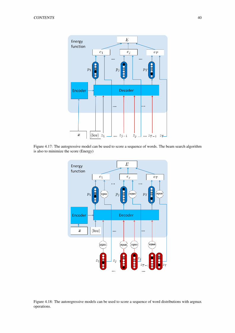
CONTENTS 40
Figure 4.17: The autogressive model can be used to score a sequence of words. The beam search algorithmis also to minimize the score (Energy)
Figure 4.18: The autoregressive models can be used to score a sequence of word distributions with argmaxoperations.
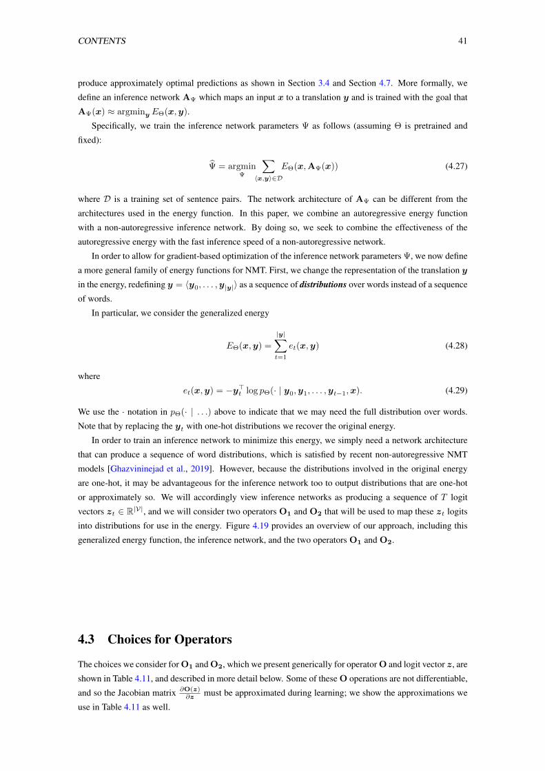
CONTENTS 41
produce approximately optimal predictions as shown in Section 3.4 and Section 4.7. More formally, we
define an inference network AΨ which maps an input x to a translation y and is trained with the goal that
AΨ(x) ≈ argminy EΘ(x,y).
Specifically, we train the inference network parameters Ψ as follows (assuming Θ is pretrained and
fixed):
Ψ = argminΨ
∑〈x,y〉∈D
EΘ(x,AΨ(x)) (4.27)
where D is a training set of sentence pairs. The network architecture of AΨ can be different from the
architectures used in the energy function. In this paper, we combine an autoregressive energy function
with a non-autoregressive inference network. By doing so, we seek to combine the effectiveness of the
autoregressive energy with the fast inference speed of a non-autoregressive network.
In order to allow for gradient-based optimization of the inference network parameters Ψ, we now define
a more general family of energy functions for NMT. First, we change the representation of the translation y
in the energy, redefining y = 〈y0, . . . ,y|y|〉 as a sequence of distributions over words instead of a sequence
of words.
In particular, we consider the generalized energy
EΘ(x,y) =
|y|∑t=1
et(x,y) (4.28)
where
et(x,y) = −y>t log pΘ(· | y0,y1, . . . ,yt−1,x). (4.29)
We use the · notation in pΘ(· | . . .) above to indicate that we may need the full distribution over words.
Note that by replacing the yt with one-hot distributions we recover the original energy.
In order to train an inference network to minimize this energy, we simply need a network architecture
that can produce a sequence of word distributions, which is satisfied by recent non-autoregressive NMT
models [Ghazvininejad et al., 2019]. However, because the distributions involved in the original energy
are one-hot, it may be advantageous for the inference network too to output distributions that are one-hot
or approximately so. We will accordingly view inference networks as producing a sequence of T logit
vectors zt ∈ R|V|, and we will consider two operators O1 and O2 that will be used to map these zt logits
into distributions for use in the energy. Figure 4.19 provides an overview of our approach, including this
generalized energy function, the inference network, and the two operators O1 and O2.
4.3 Choices for Operators
The choices we consider for O1 and O2, which we present generically for operator O and logit vector z, are
shown in Table 4.11, and described in more detail below. Some of these O operations are not differentiable,
and so the Jacobian matrix ∂O(z)∂z must be approximated during learning; we show the approximations we
use in Table 4.11 as well.
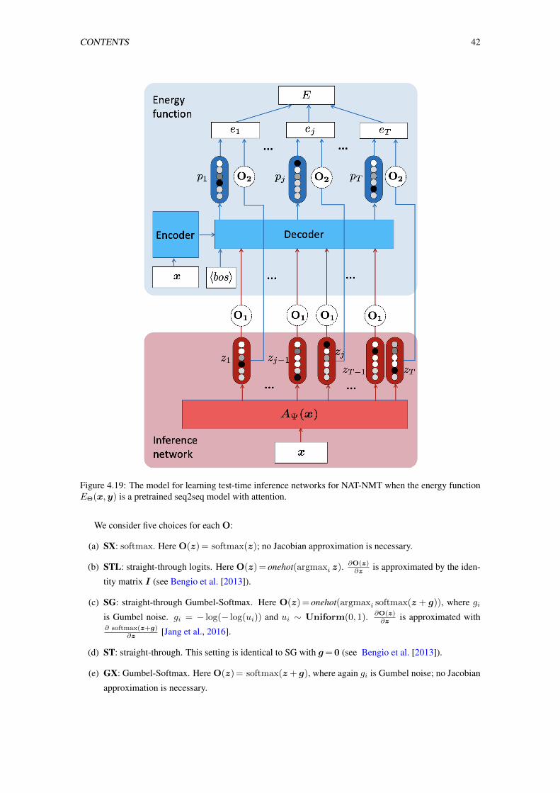
CONTENTS 42
Figure 4.19: The model for learning test-time inference networks for NAT-NMT when the energy functionEΘ(x,y) is a pretrained seq2seq model with attention.
We consider five choices for each O:
(a) SX: softmax. Here O(z) = softmax(z); no Jacobian approximation is necessary.
(b) STL: straight-through logits. Here O(z) = onehot(argmaxi z). ∂O(z)∂z is approximated by the iden-
tity matrix I (see Bengio et al. [2013]).
(c) SG: straight-through Gumbel-Softmax. Here O(z) = onehot(argmaxi softmax(z + g)), where giis Gumbel noise. gi = − log(− log(ui)) and ui ∼ Uniform(0, 1). ∂O(z)
∂z is approximated with∂ softmax(z+g)
∂z [Jang et al., 2016].
(d) ST: straight-through. This setting is identical to SG with g =0 (see Bengio et al. [2013]).
(e) GX: Gumbel-Softmax. Here O(z) = softmax(z + g), where again gi is Gumbel noise; no Jacobian
approximation is necessary.
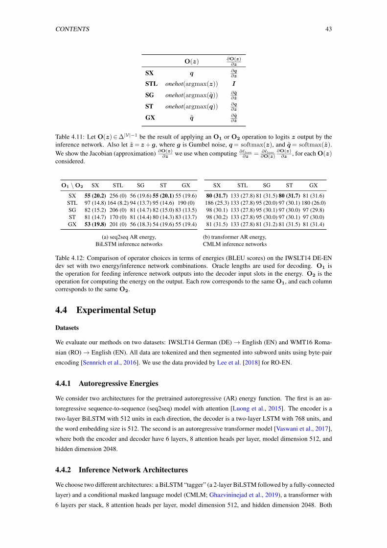
CONTENTS 43
O(z) ∂O(z)∂z
SX q ∂q∂z
STL onehot(argmax(z)) I
SG onehot(argmax(q)) ∂q∂z
ST onehot(argmax(q)) ∂q∂z
GX q ∂q∂z
Table 4.11: Let O(z)∈∆|V|−1 be the result of applying an O1 or O2 operation to logits z output by theinference network. Also let z = z + g, where g is Gumbel noise, q = softmax(z), and q = softmax(z).We show the Jacobian (approximation) ∂O(z)
∂z we use when computing ∂`loss
∂z = ∂`loss
∂O(z)∂O(z)∂z , for each O(z)
considered.
O1 \O2 SX STL SG ST GX
SX 55 (20.2) 256 (0) 56 (19.6) 55 (20.1) 55 (19.6)STL 97 (14.8) 164 (8.2) 94 (13.7) 95 (14.6) 190 (0)SG 82 (15.2) 206 (0) 81 (14.7) 82 (15.0) 83 (13.5)ST 81 (14.7) 170 (0) 81 (14.4) 80 (14.3) 83 (13.7)GX 53 (19.8) 201 (0) 56 (18.3) 54 (19.6) 55 (19.4)
(a) seq2seq AR energy,BiLSTM inference networks
SX STL SG ST GX
80 (31.7) 133 (27.8) 81 (31.5) 80 (31.7) 81 (31.6)186 (25.3) 133 (27.8) 95 (20.0) 97 (30.1) 180 (26.0)98 (30.1) 133 (27.8) 95 (30.1) 97 (30.0) 97 (29.8)98 (30.2) 133 (27.8) 95 (30.0) 97 (30.1) 97 (30.0)81 (31.5) 133 (27.8) 81 (31.2) 81 (31.5) 81 (31.4)
(b) transformer AR energy,CMLM inference networks
Table 4.12: Comparison of operator choices in terms of energies (BLEU scores) on the IWSLT14 DE-ENdev set with two energy/inference network combinations. Oracle lengths are used for decoding. O1 isthe operation for feeding inference network outputs into the decoder input slots in the energy. O2 is theoperation for computing the energy on the output. Each row corresponds to the same O1, and each columncorresponds to the same O2.
4.4 Experimental Setup
Datasets
We evaluate our methods on two datasets: IWSLT14 German (DE)→ English (EN) and WMT16 Roma-
nian (RO)→ English (EN). All data are tokenized and then segmented into subword units using byte-pair
encoding [Sennrich et al., 2016]. We use the data provided by Lee et al. [2018] for RO-EN.
4.4.1 Autoregressive Energies
We consider two architectures for the pretrained autoregressive (AR) energy function. The first is an au-
toregressive sequence-to-sequence (seq2seq) model with attention [Luong et al., 2015]. The encoder is a
two-layer BiLSTM with 512 units in each direction, the decoder is a two-layer LSTM with 768 units, and
the word embedding size is 512. The second is an autoregressive transformer model [Vaswani et al., 2017],
where both the encoder and decoder have 6 layers, 8 attention heads per layer, model dimension 512, and
hidden dimension 2048.
4.4.2 Inference Network Architectures
We choose two different architectures: a BiLSTM “tagger” (a 2-layer BiLSTM followed by a fully-connected
layer) and a conditional masked language model (CMLM; Ghazvininejad et al., 2019), a transformer with
6 layers per stack, 8 attention heads per layer, model dimension 512, and hidden dimension 2048. Both
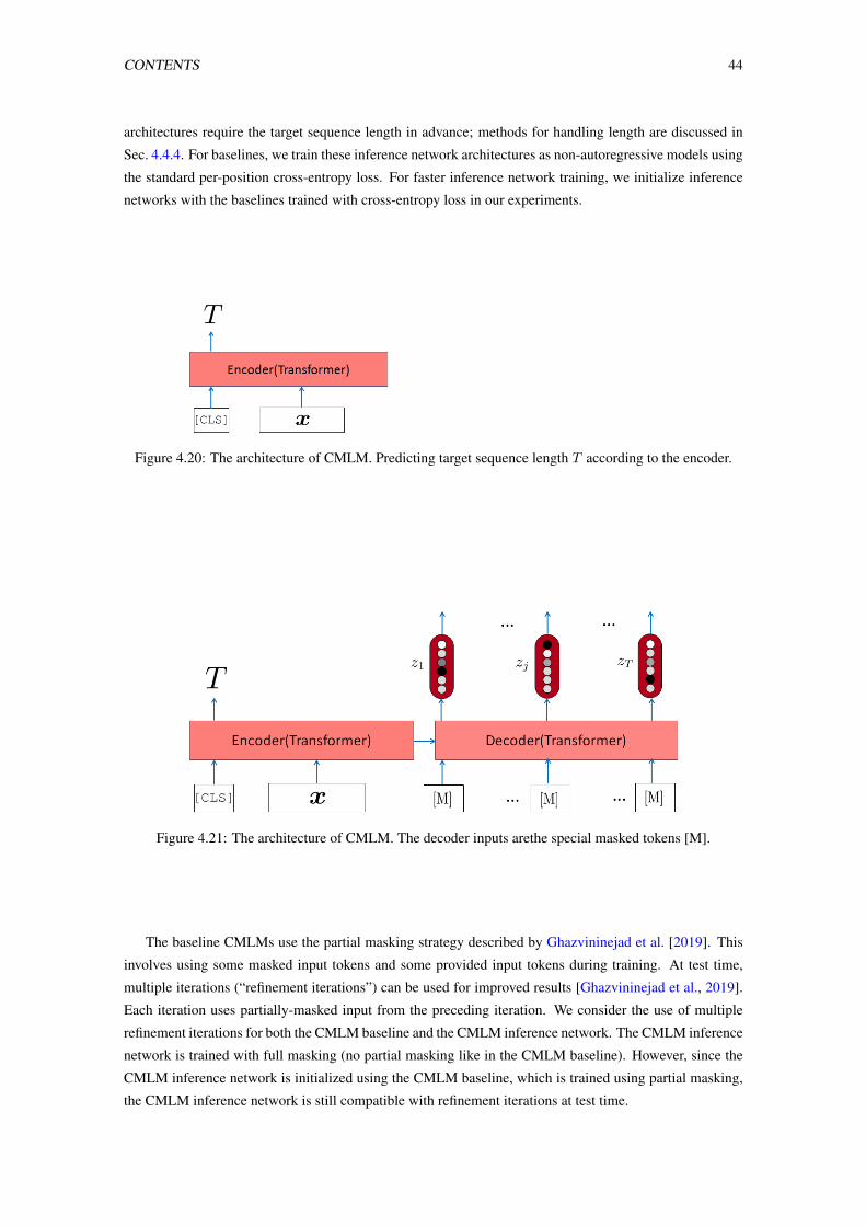
CONTENTS 44
architectures require the target sequence length in advance; methods for handling length are discussed in
Sec. 4.4.4. For baselines, we train these inference network architectures as non-autoregressive models using
the standard per-position cross-entropy loss. For faster inference network training, we initialize inference
networks with the baselines trained with cross-entropy loss in our experiments.
Figure 4.20: The architecture of CMLM. Predicting target sequence length T according to the encoder.
Figure 4.21: The architecture of CMLM. The decoder inputs arethe special masked tokens [M].
The baseline CMLMs use the partial masking strategy described by Ghazvininejad et al. [2019]. This
involves using some masked input tokens and some provided input tokens during training. At test time,
multiple iterations (“refinement iterations”) can be used for improved results [Ghazvininejad et al., 2019].
Each iteration uses partially-masked input from the preceding iteration. We consider the use of multiple
refinement iterations for both the CMLM baseline and the CMLM inference network. The CMLM inference
network is trained with full masking (no partial masking like in the CMLM baseline). However, since the
CMLM inference network is initialized using the CMLM baseline, which is trained using partial masking,
the CMLM inference network is still compatible with refinement iterations at test time.
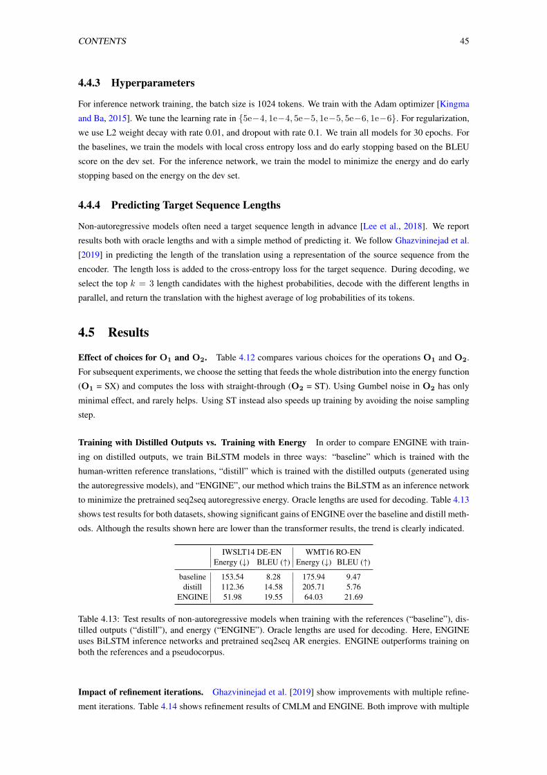
CONTENTS 45
4.4.3 Hyperparameters
For inference network training, the batch size is 1024 tokens. We train with the Adam optimizer [Kingma
and Ba, 2015]. We tune the learning rate in {5e−4, 1e−4, 5e−5, 1e−5, 5e−6, 1e−6}. For regularization,
we use L2 weight decay with rate 0.01, and dropout with rate 0.1. We train all models for 30 epochs. For
the baselines, we train the models with local cross entropy loss and do early stopping based on the BLEU
score on the dev set. For the inference network, we train the model to minimize the energy and do early
stopping based on the energy on the dev set.
4.4.4 Predicting Target Sequence Lengths
Non-autoregressive models often need a target sequence length in advance [Lee et al., 2018]. We report
results both with oracle lengths and with a simple method of predicting it. We follow Ghazvininejad et al.
[2019] in predicting the length of the translation using a representation of the source sequence from the
encoder. The length loss is added to the cross-entropy loss for the target sequence. During decoding, we
select the top k = 3 length candidates with the highest probabilities, decode with the different lengths in
parallel, and return the translation with the highest average of log probabilities of its tokens.
4.5 Results
Effect of choices for O1 and O2. Table 4.12 compares various choices for the operations O1 and O2.
For subsequent experiments, we choose the setting that feeds the whole distribution into the energy function
(O1 = SX) and computes the loss with straight-through (O2 = ST). Using Gumbel noise in O2 has only
minimal effect, and rarely helps. Using ST instead also speeds up training by avoiding the noise sampling
step.
Training with Distilled Outputs vs. Training with Energy In order to compare ENGINE with train-
ing on distilled outputs, we train BiLSTM models in three ways: “baseline” which is trained with the
human-written reference translations, “distill” which is trained with the distilled outputs (generated using
the autoregressive models), and “ENGINE”, our method which trains the BiLSTM as an inference network
to minimize the pretrained seq2seq autoregressive energy. Oracle lengths are used for decoding. Table 4.13
shows test results for both datasets, showing significant gains of ENGINE over the baseline and distill meth-
ods. Although the results shown here are lower than the transformer results, the trend is clearly indicated.
IWSLT14 DE-EN WMT16 RO-ENEnergy (↓) BLEU (↑) Energy (↓) BLEU (↑)
baseline 153.54 8.28 175.94 9.47distill 112.36 14.58 205.71 5.76
ENGINE 51.98 19.55 64.03 21.69
Table 4.13: Test results of non-autoregressive models when training with the references (“baseline”), dis-tilled outputs (“distill”), and energy (“ENGINE”). Oracle lengths are used for decoding. Here, ENGINEuses BiLSTM inference networks and pretrained seq2seq AR energies. ENGINE outperforms training onboth the references and a pseudocorpus.
Impact of refinement iterations. Ghazvininejad et al. [2019] show improvements with multiple refine-
ment iterations. Table 4.14 shows refinement results of CMLM and ENGINE. Both improve with multiple
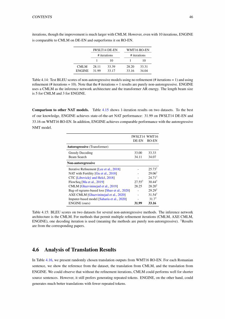
CONTENTS 46
iterations, though the improvement is much larger with CMLM. However, even with 10 iterations, ENGINE
is comparable to CMLM on DE-EN and outperforms it on RO-EN.
IWSLT14 DE-EN WMT16 RO-EN
# iterations # iterations
1 10 1 10
CMLM 28.11 33.39 28.20 33.31ENGINE 31.99 33.17 33.16 34.04
Table 4.14: Test BLEU scores of non-autoregressive models using no refinement (# iterations = 1) and usingrefinement (# iterations = 10). Note that the # iterations = 1 results are purely non-autoregressive. ENGINEuses a CMLM as the inference network architecture and the transformer AR energy. The length beam sizeis 5 for CMLM and 3 for ENGINE.
Comparison to other NAT models. Table 4.15 shows 1-iteration results on two datasets. To the best
of our knowledge, ENGINE achieves state-of-the-art NAT performance: 31.99 on IWSLT14 DE-EN and
33.16 on WMT16 RO-EN. In addition, ENGINE achieves comparable performance with the autoregressive
NMT model.
IWSLT14 WMT16DE-EN RO-EN
Autoregressive (Transformer)
Greedy Decoding 33.00 33.33Beam Search 34.11 34.07
Non-autoregressive
Iterative Refinement [Lee et al., 2018] - 25.73†
NAT with Fertility [Gu et al., 2018] - 29.06†
CTC [Libovický and Helcl, 2018] - 24.71†
FlowSeq [Ma et al., 2019] 27.55† 30.44†
CMLM [Ghazvininejad et al., 2019] 28.25 28.20†
Bag-of-ngrams-based loss [Shao et al., 2020] - 29.29†
AXE CMLM [Ghazvininejad et al., 2020] - 31.54†
Imputer-based model [Saharia et al., 2020] - 31.7†
ENGINE (ours) 31.99 33.16
Table 4.15: BLEU scores on two datasets for several non-autoregressive methods. The inference networkarchitecture is the CMLM. For methods that permit multiple refinement iterations (CMLM, AXE CMLM,ENGINE), one decoding iteration is used (meaning the methods are purely non-autoregressive). †Resultsare from the corresponding papers.
4.6 Analysis of Translation Results
In Table 4.16, we present randomly chosen translation outputs from WMT16 RO-EN. For each Romanian
sentence, we show the reference from the dataset, the translation from CMLM, and the translation from
ENGINE. We could observe that without the refinement iterations, CMLM could performs well for shorter
source sentences. However, it still prefers generating repeated tokens. ENGINE, on the other hand, could
generates much better translations with fewer repeated tokens.
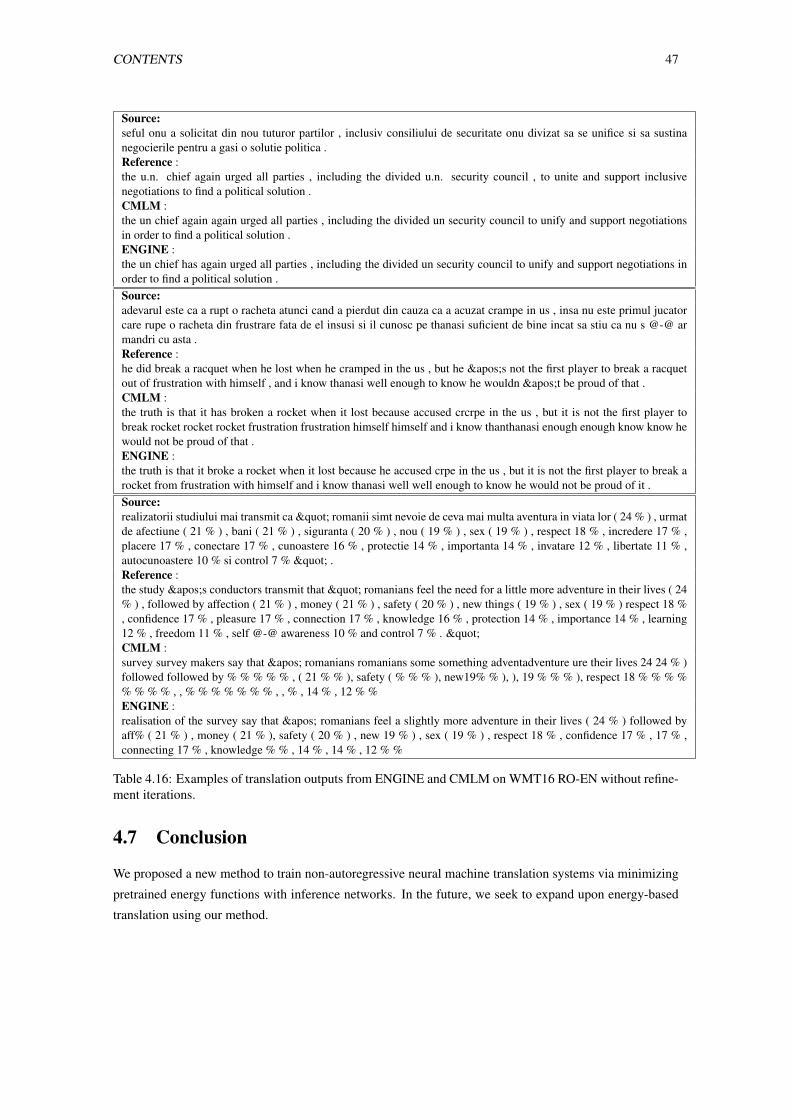
CONTENTS 47
Source:seful onu a solicitat din nou tuturor partilor , inclusiv consiliului de securitate onu divizat sa se unifice si sa sustinanegocierile pentru a gasi o solutie politica .Reference :the u.n. chief again urged all parties , including the divided u.n. security council , to unite and support inclusivenegotiations to find a political solution .CMLM :the un chief again again urged all parties , including the divided un security council to unify and support negotiationsin order to find a political solution .ENGINE :the un chief has again urged all parties , including the divided un security council to unify and support negotiations inorder to find a political solution .Source:adevarul este ca a rupt o racheta atunci cand a pierdut din cauza ca a acuzat crampe in us , insa nu este primul jucatorcare rupe o racheta din frustrare fata de el insusi si il cunosc pe thanasi suficient de bine incat sa stiu ca nu s @-@ armandri cu asta .Reference :he did break a racquet when he lost when he cramped in the us , but he 's not the first player to break a racquetout of frustration with himself , and i know thanasi well enough to know he wouldn 't be proud of that .CMLM :the truth is that it has broken a rocket when it lost because accused crcrpe in the us , but it is not the first player tobreak rocket rocket rocket frustration frustration himself himself and i know thanthanasi enough enough know know hewould not be proud of that .ENGINE :the truth is that it broke a rocket when it lost because he accused crpe in the us , but it is not the first player to break arocket from frustration with himself and i know thanasi well well enough to know he would not be proud of it .Source:realizatorii studiului mai transmit ca " romanii simt nevoie de ceva mai multa aventura in viata lor ( 24 % ) , urmatde afectiune ( 21 % ) , bani ( 21 % ) , siguranta ( 20 % ) , nou ( 19 % ) , sex ( 19 % ) , respect 18 % , incredere 17 % ,placere 17 % , conectare 17 % , cunoastere 16 % , protectie 14 % , importanta 14 % , invatare 12 % , libertate 11 % ,autocunoastere 10 % si control 7 % " .Reference :the study 's conductors transmit that " romanians feel the need for a little more adventure in their lives ( 24% ) , followed by affection ( 21 % ) , money ( 21 % ) , safety ( 20 % ) , new things ( 19 % ) , sex ( 19 % ) respect 18 %, confidence 17 % , pleasure 17 % , connection 17 % , knowledge 16 % , protection 14 % , importance 14 % , learning12 % , freedom 11 % , self @-@ awareness 10 % and control 7 % . "CMLM :survey survey makers say that ' romanians romanians some something adventadventure ure their lives 24 24 % )followed followed by % % % % % , ( 21 % % ), safety ( % % % ), new19% % ), ), 19 % % % ), respect 18 % % % %% % % % , , % % % % % % % , , % , 14 % , 12 % %ENGINE :realisation of the survey say that ' romanians feel a slightly more adventure in their lives ( 24 % ) followed byaff% ( 21 % ) , money ( 21 % ), safety ( 20 % ) , new 19 % ) , sex ( 19 % ) , respect 18 % , confidence 17 % , 17 % ,connecting 17 % , knowledge % % , 14 % , 14 % , 12 % %
Table 4.16: Examples of translation outputs from ENGINE and CMLM on WMT16 RO-EN without refine-ment iterations.
4.7 Conclusion
We proposed a new method to train non-autoregressive neural machine translation systems via minimizing
pretrained energy functions with inference networks. In the future, we seek to expand upon energy-based
translation using our method.
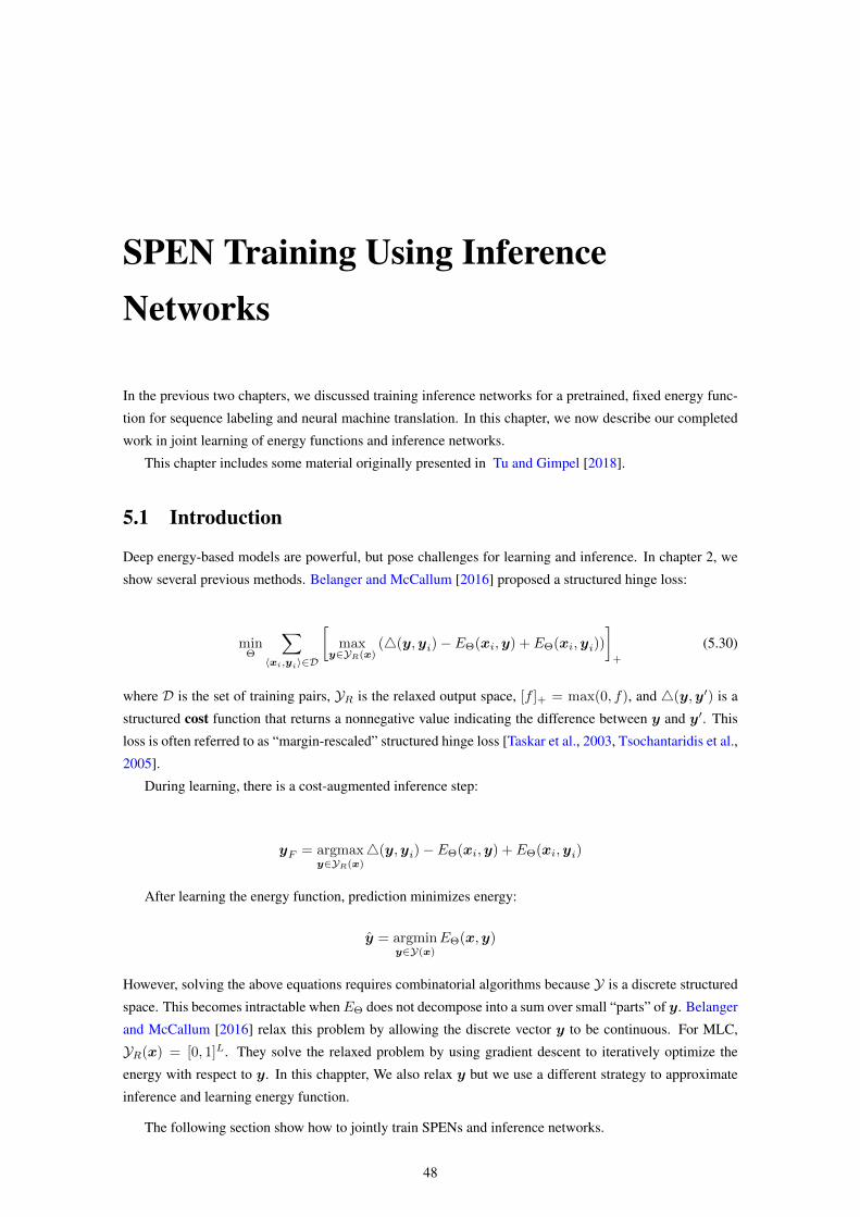
SPEN Training Using InferenceNetworks
In the previous two chapters, we discussed training inference networks for a pretrained, fixed energy func-
tion for sequence labeling and neural machine translation. In this chapter, we now describe our completed
work in joint learning of energy functions and inference networks.
This chapter includes some material originally presented in Tu and Gimpel [2018].
5.1 Introduction
Deep energy-based models are powerful, but pose challenges for learning and inference. In chapter 2, we
show several previous methods. Belanger and McCallum [2016] proposed a structured hinge loss:
minΘ
∑〈xi,yi〉∈D
[max
y∈YR(x)(4(y,yi)− EΘ(xi,y) + EΘ(xi,yi))
]+
(5.30)
where D is the set of training pairs, YR is the relaxed output space, [f ]+ = max(0, f), and 4(y,y′) is a
structured cost function that returns a nonnegative value indicating the difference between y and y′. This
loss is often referred to as “margin-rescaled” structured hinge loss [Taskar et al., 2003, Tsochantaridis et al.,
2005].
During learning, there is a cost-augmented inference step:
yF = argmaxy∈YR(x)
4(y,yi)− EΘ(xi,y) + EΘ(xi,yi)
After learning the energy function, prediction minimizes energy:
y = argminy∈Y(x)
EΘ(x,y)
However, solving the above equations requires combinatorial algorithms because Y is a discrete structured
space. This becomes intractable whenEΘ does not decompose into a sum over small “parts” of y. Belanger
and McCallum [2016] relax this problem by allowing the discrete vector y to be continuous. For MLC,
YR(x) = [0, 1]L. They solve the relaxed problem by using gradient descent to iteratively optimize the
energy with respect to y. In this chappter, We also relax y but we use a different strategy to approximate
inference and learning energy function.
The following section show how to jointly train SPENs and inference networks.
48
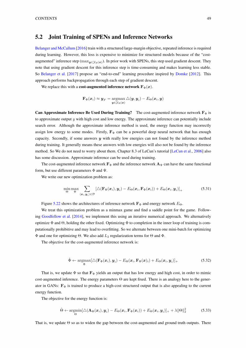
CONTENTS 49
5.2 Joint Training of SPENs and Inference Networks
Belanger and McCallum [2016] train with a structured large-margin objective, repeated inference is required
during learning. However, this loss is expensive to minimize for structured models because of the “cost-
augmented” inference step (maxy∈YR(x)). In prior work with SPENs, this step used gradient descent. They
note that using gradient descent for this inference step is time-consuming and makes learning less stable.
So Belanger et al. [2017] propose an “end-to-end” learning procedure inspired by Domke [2012]. This
approach performs backpropagation through each step of gradient descent.
We replace this with a cost-augmented inference network FΦ(x).
FΦ(xi) ≈ yF = argmaxy∈YR(x)
4(y,yi)− EΘ(xi,y)
Can Approximate Inference Be Used During Training? The cost-augmented inference network FΦ is
to approximate output y with high cost and low energy. The approximate inference can potentially include
search error. Although the approximate inference method is used, the energy function may incorrectly
assign low energy to some modes. Firstly, FΦ can be a powerful deep neural network that has enough
capacity. Secondly, if some answers y with really low energies can not found by the inference method
during training. It generally means these answers with low energies will also not be found by the inference
method. So We do not need to worry about them. Chapter 8.3 of LeCun’s tutorial [LeCun et al., 2006] also
has some discussion. Approximate inference can be used during training.
The cost-augmented inference network FΦ and the inference network AΨ can have the same functional
form, but use different parameters Φ and Ψ.
We write our new optimization problem as:
minΘ
maxΦ
∑〈xi,yi〉∈D
[4(FΦ(xi),yi)− EΘ(xi,FΦ(xi)) + EΘ(xi,yi)]+ (5.31)
Figure 5.22 shows the architectures of inference network FΦ and energy network EΘ.
We treat this optimization problem as a minmax game and find a saddle point for the game. Follow-
ing Goodfellow et al. [2014], we implement this using an iterative numerical approach. We alternatively
optimize Φ and Θ, holding the other fixed. Optimizing Φ to completion in the inner loop of training is com-
putationally prohibitive and may lead to overfitting. So we alternate between one mini-batch for optimizing
Φ and one for optimizing Θ. We also add L2 regularization terms for Θ and Φ.
The objective for the cost-augmented inference network is:
Φ← argmaxΦ
[4(FΦ(xi),yi)− EΘ(xi,FΦ(x)i) + EΘ(xi,yi)]+ (5.32)
That is, we update Φ so that FΦ yields an output that has low energy and high cost, in order to mimic
cost-augmented inference. The energy parameters Θ are kept fixed. There is an analogy here to the gener-
ator in GANs: FΦ is trained to produce a high-cost structured output that is also appealing to the current
energy function.
The objective for the energy function is:
Θ← argminΘ
[4(AΦ(xi),yi)− EΘ(xi,FΦ(xi)) + EΘ(xi,yi)]+ + λ‖Θ‖22 (5.33)
That is, we update Θ so as to widen the gap between the cost-augmented and ground truth outputs. There
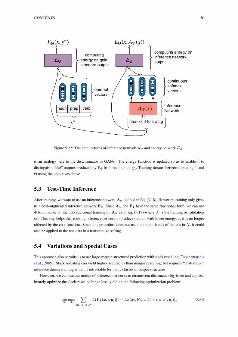
CONTENTS 50
Figure 5.22: The architectures of inference network AΨ and energy network EΘ.
is an analogy here to the discriminator in GANs. The energy function is updated so as to enable it to
distinguish “fake” outputs produced by FΦ from real outputs yi. Training iterates between updating Φ and
Θ using the objectives above.
5.3 Test-Time Inference
After training, we want to use an inference network AΨ defined in Eq. (3.18). However, training only gives
us a cost-augmented inference network FΦ. Since AΨ and FΦ have the same functional form, we can use
Φ to initialize Ψ, then do additional training on AΨ as in Eq. (3.19) where X is the training or validation
set. This step helps the resulting inference network to produce outputs with lower energy, as it is no longer
affected by the cost function. Since this procedure does not use the output labels of the x’s in X , it could
also be applied to the test data in a transductive setting.
5.4 Variations and Special Cases
This approach also permits us to use large-margin structured prediction with slack rescaling [Tsochantaridis
et al., 2005]. Slack rescaling can yield higher accuracies than margin rescaling, but requires “cost-scaled”
inference during training which is intractable for many classes of output structures.
However, we can use our notion of inference networks to circumvent this tractability issue and approx-
imately optimize the slack-rescaled hinge loss, yielding the following optimization problem:
minΘ
maxΦ
∑〈xi,yi〉∈D
4(FΦ(xi),yi)[1− EΘ(xi,FΦ(xi)) + EΘ(xi,yi)]+ (5.34)
CONTENTS 51
Using the same argument as above, we can also break this into alternating optimization of Φ and Θ.
We can optimize a structured perceptron [Collins, 2002] version by using the margin-rescaled hinge loss
(Eq. (6.40)) and fixing 4(FΦ(xi),yi) = 0. When using this loss, the cost-augmented inference network
is actually a test-time inference network, because the cost is always zero, so using this loss may lessen the
need to retune the inference network after training.
When we fix 4(FΦ(xi),yi) = 1, then margin-rescaled hinge is equivalent to slack-rescaled hinge.
While using 4 = 1 is not useful in standard max-margin training with exact argmax inference (because
the cost has no impact on optimization when fixed to a positive constant), it is potentially useful in our
setting.
Consider our SPEN objectives with4 = 1:
[1− EΘ(xi,FΦ(xi)) + EΘ(xi,yi)]+ (5.35)
There will always be a nonzero difference between the two energies because FΦ(xi) will never exactly
equal the discrete vector yi.
Since there is no explicit minimization over all discrete vectors y, this case is more similar to a “con-
trastive” hinge loss which seeks to make the energy of the true output lower than the energy of a particular
“negative sample” by a margin of at least 1.
5.5 Improving Training for Inference Networks
We found that the alternating nature of the optimization led to difficulties during training. Similar observa-
tions have been noted about other alternative optimization settings, especially those underlying generative
adversarial networks [Salimans et al., 2016].
Below we describe several techniques we found to help stabilize training, which are optional terms
added to the objective in Eq. (5.32).
L2 Regularization: We use L2 regularization, adding the penalty term ‖Φ‖22 with coefficient λ1.
Entropy Regularization: We add an entropy-based regularizer lossH(FΦ(x)) defined for the problem
under consideration. For MLC, the output of FΦ(x) is a vector of scalars in [0, 1], one for each label, where
the scalar is interpreted as a label probability. The entropy regularizer lossH is the sum of the entropies over
these label binary distributions.
For sequence labeling, where the length of x is N and where there are L unique labels, the output of
FΦ(x) is a length-N sequence of length-L vectors, each of which represents the distribution over the L
labels at that position in x. Then, lossH is the sum of entropies of these label distributions across positions
in the sequence.
When tuning the coefficient λ2 for this regularizer, we consider both positive and negative values,
permitting us to favor either low- or high-entropy distributions as the task prefers.6
Local Cross Entropy Loss: We add a local (non-structured) cross entropy lossCE(FΦ(xi),yi) defined
for the problem under consideration. We only experiment with this loss for sequence labeling.
It is the sum of the label cross entropy losses over all positions in the sequence. This loss provides
more explicit feedback to the inference network, helping the optimization procedure to find a solution that
minimizes the energy function while also correctly classifying individual labels. It can also be viewed as a
multi-task loss for the inference network.6For MLC, encouraging lower entropy distributions worked better, while for sequence labeling, higher entropy was better, similar
to the effect found by Pereyra et al. [2017]. Further research is required to gain understanding of the role of entropy regularization insuch alternating optimization settings.
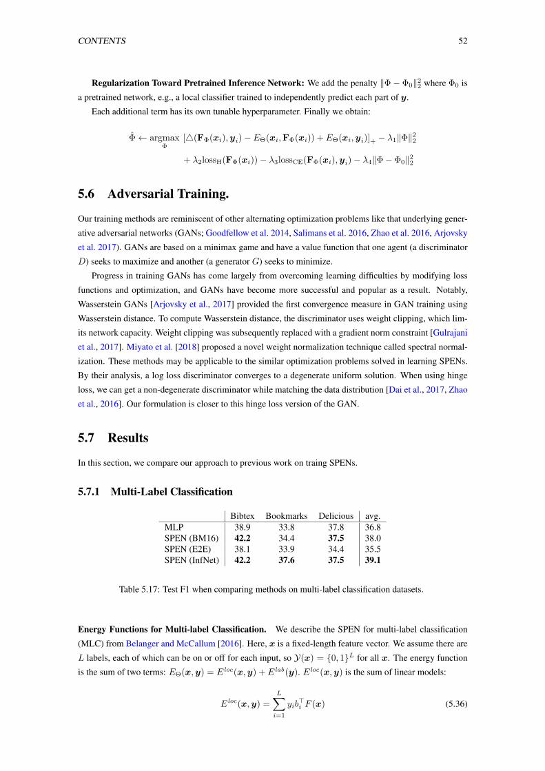
CONTENTS 52
Regularization Toward Pretrained Inference Network: We add the penalty ‖Φ− Φ0‖22 where Φ0 is
a pretrained network, e.g., a local classifier trained to independently predict each part of y.
Each additional term has its own tunable hyperparameter. Finally we obtain:
Φ← argmaxΦ
[4(FΦ(xi),yi)− EΘ(xi,FΦ(xi)) + EΘ(xi,yi)]+ − λ1‖Φ‖22
+ λ2lossH(FΦ(xi))− λ3lossCE(FΦ(xi),yi)− λ4‖Φ− Φ0‖22
5.6 Adversarial Training.
Our training methods are reminiscent of other alternating optimization problems like that underlying gener-
ative adversarial networks (GANs; Goodfellow et al. 2014, Salimans et al. 2016, Zhao et al. 2016, Arjovsky
et al. 2017). GANs are based on a minimax game and have a value function that one agent (a discriminator
D) seeks to maximize and another (a generator G) seeks to minimize.
Progress in training GANs has come largely from overcoming learning difficulties by modifying loss
functions and optimization, and GANs have become more successful and popular as a result. Notably,
Wasserstein GANs [Arjovsky et al., 2017] provided the first convergence measure in GAN training using
Wasserstein distance. To compute Wasserstein distance, the discriminator uses weight clipping, which lim-
its network capacity. Weight clipping was subsequently replaced with a gradient norm constraint [Gulrajani
et al., 2017]. Miyato et al. [2018] proposed a novel weight normalization technique called spectral normal-
ization. These methods may be applicable to the similar optimization problems solved in learning SPENs.
By their analysis, a log loss discriminator converges to a degenerate uniform solution. When using hinge
loss, we can get a non-degenerate discriminator while matching the data distribution [Dai et al., 2017, Zhao
et al., 2016]. Our formulation is closer to this hinge loss version of the GAN.
5.7 Results
In this section, we compare our approach to previous work on traing SPENs.
5.7.1 Multi-Label Classification
Bibtex Bookmarks Delicious avg.MLP 38.9 33.8 37.8 36.8SPEN (BM16) 42.2 34.4 37.5 38.0SPEN (E2E) 38.1 33.9 34.4 35.5SPEN (InfNet) 42.2 37.6 37.5 39.1
Table 5.17: Test F1 when comparing methods on multi-label classification datasets.
Energy Functions for Multi-label Classification. We describe the SPEN for multi-label classification
(MLC) from Belanger and McCallum [2016]. Here, x is a fixed-length feature vector. We assume there are
L labels, each of which can be on or off for each input, so Y(x) = {0, 1}L for all x. The energy function
is the sum of two terms: EΘ(x,y) = Eloc(x,y) + Elab(y). Eloc(x,y) is the sum of linear models:
Eloc(x,y) =
L∑i=1
yib>i F (x) (5.36)
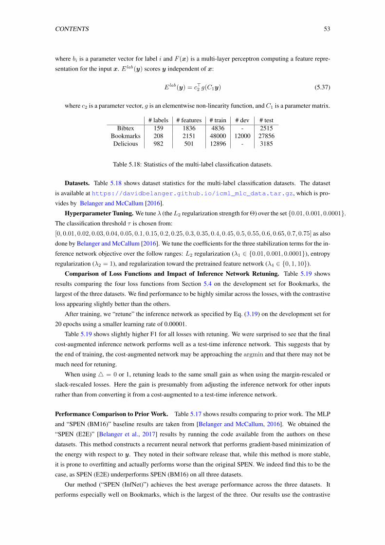
CONTENTS 53
where bi is a parameter vector for label i and F (x) is a multi-layer perceptron computing a feature repre-
sentation for the input x. Elab(y) scores y independent of x:
Elab(y) = c>2 g(C1y) (5.37)
where c2 is a parameter vector, g is an elementwise non-linearity function, andC1 is a parameter matrix.
# labels # features # train # dev # testBibtex 159 1836 4836 - 2515
Bookmarks 208 2151 48000 12000 27856Delicious 982 501 12896 - 3185
Table 5.18: Statistics of the multi-label classification datasets.
Datasets. Table 5.18 shows dataset statistics for the multi-label classification datasets. The dataset
is available at https://davidbelanger.github.io/icml_mlc_data.tar.gz, which is pro-
vides by Belanger and McCallum [2016].
Hyperparameter Tuning. We tune λ (theL2 regularization strength for Θ) over the set {0.01, 0.001, 0.0001}.The classification threshold τ is chosen from:
[0, 0.01, 0.02, 0.03, 0.04, 0.05, 0.1, 0.15, 0.2, 0.25, 0.3, 0.35, 0.4, 0.45, 0.5, 0.55, 0.6, 0.65, 0.7, 0.75] as also
done by Belanger and McCallum [2016]. We tune the coefficients for the three stabilization terms for the in-
ference network objective over the follow ranges: L2 regularization (λ1 ∈ {0.01, 0.001, 0.0001}), entropy
regularization (λ2 = 1), and regularization toward the pretrained feature network (λ4 ∈ {0, 1, 10}).Comparison of Loss Functions and Impact of Inference Network Retuning. Table 5.19 shows
results comparing the four loss functions from Section 5.4 on the development set for Bookmarks, the
largest of the three datasets. We find performance to be highly similar across the losses, with the contrastive
loss appearing slightly better than the others.
After training, we “retune” the inference network as specified by Eq. (3.19) on the development set for
20 epochs using a smaller learning rate of 0.00001.
Table 5.19 shows slightly higher F1 for all losses with retuning. We were surprised to see that the final
cost-augmented inference network performs well as a test-time inference network. This suggests that by
the end of training, the cost-augmented network may be approaching the argmin and that there may not be
much need for retuning.
When using 4 = 0 or 1, retuning leads to the same small gain as when using the margin-rescaled or
slack-rescaled losses. Here the gain is presumably from adjusting the inference network for other inputs
rather than from converting it from a cost-augmented to a test-time inference network.
Performance Comparison to Prior Work. Table 5.17 shows results comparing to prior work. The MLP
and “SPEN (BM16)” baseline results are taken from [Belanger and McCallum, 2016]. We obtained the
“SPEN (E2E)” [Belanger et al., 2017] results by running the code available from the authors on these
datasets. This method constructs a recurrent neural network that performs gradient-based minimization of
the energy with respect to y. They noted in their software release that, while this method is more stable,
it is prone to overfitting and actually performs worse than the original SPEN. We indeed find this to be the
case, as SPEN (E2E) underperforms SPEN (BM16) on all three datasets.
Our method (“SPEN (InfNet)”) achieves the best average performance across the three datasets. It
performs especially well on Bookmarks, which is the largest of the three. Our results use the contrastive
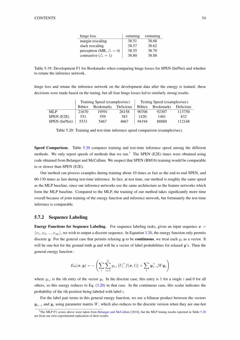
CONTENTS 54
hinge loss -retuning +retuningmargin rescaling 38.51 38.68slack rescaling 38.57 38.62perceptron (MR,4 = 0) 38.55 38.70contrastive (4 = 1) 38.80 38.88
Table 5.19: Development F1 for Bookmarks when comparing hinge losses for SPEN (InfNet) and whetherto retune the inference network.
hinge loss and retune the inference network on the development data after the energy is trained; these
decisions were made based on the tuning, but all four hinge losses led to similarly strong results.
Training Speed (examples/sec) Testing Speed (examples/sec)Bibtex Bookmarks Delicious Bibtex Bookmarks Delicious
MLP 21670 19591 26158 90706 92307 113750SPEN (E2E) 551 559 383 1420 1401 832SPEN (InfNet) 5533 5467 4667 94194 88888 112148
Table 5.20: Training and test-time inference speed comparison (examples/sec).
Speed Comparison. Table 5.20 compares training and test-time inference speed among the different
methods. We only report speeds of methods that we ran.7 The SPEN (E2E) times were obtained using
code obtained from Belanger and McCallum. We suspect that SPEN (BM16) training would be comparable
to or slower than SPEN (E2E).
Our method can process examples during training about 10 times as fast as the end-to-end SPEN, and
60-130 times as fast during test-time inference. In fact, at test time, our method is roughly the same speed
as the MLP baseline, since our inference networks use the same architecture as the feature networks which
form the MLP baseline. Compared to the MLP, the training of our method takes significantly more time
overall because of joint training of the energy function and inference network, but fortunately the test-time
inference is comparable.
5.7.2 Sequence Labeling
Energy Functions for Sequence Labeling. For sequence labeling tasks, given an input sequence x =
〈x1, x2, ..., x|x|〉, we wish to output a discrete sequence. In Equation 3.20, the energy function only permits
discrete y. For the general case that permits relaxing y to be continuous, we treat each yt as a vector. It
will be one-hot for the ground truth y and will be a vector of label probabilities for relaxed y’s. Then the
general energy function :
EΘ(x,y) = −
(∑t
L∑i=1
yt,i(U>i f(x, t)
)+∑t
y>t−1Wyt
)
where yt,i is the ith entry of the vector yt. In the discrete case, this entry is 1 for a single i and 0 for all
others, so this energy reduces to Eq. (3.20) in that case. In the continuous case, this scalar indicates the
probability of the tth position being labeled with label i.
For the label pair terms in this general energy function, we use a bilinear product between the vectors
yt−1 and yt using parameter matrix W , which also reduces to the discrete version when they are one-hot
7The MLP F1 scores above were taken from Belanger and McCallum [2016], but the MLP timing results reported in Table 5.20are from our own experimental replication of their results.
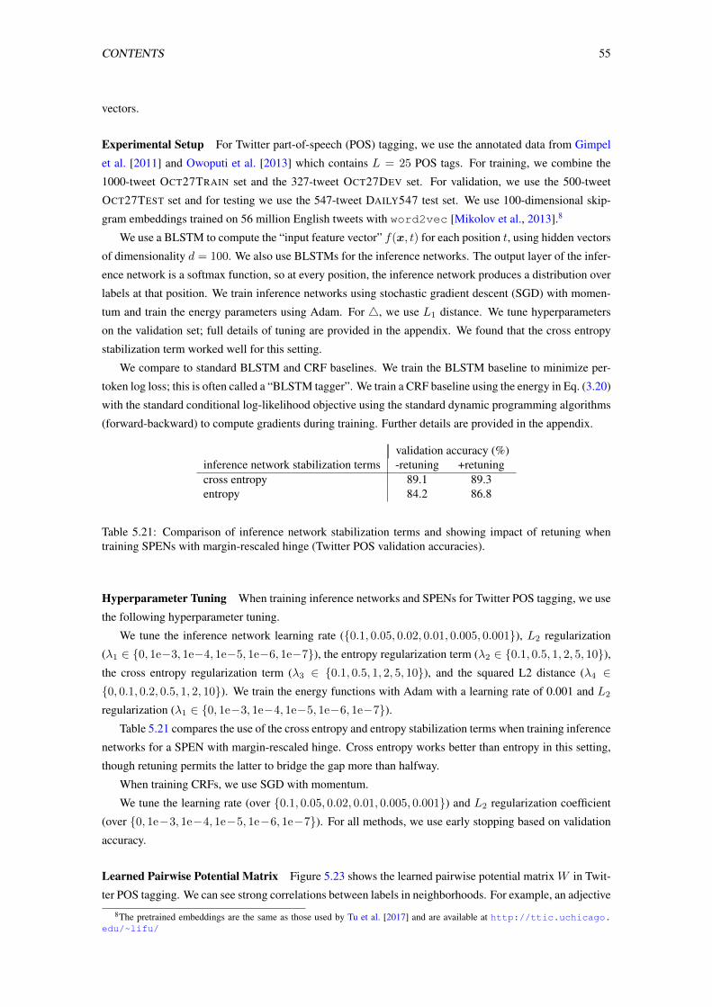
CONTENTS 55
vectors.
Experimental Setup For Twitter part-of-speech (POS) tagging, we use the annotated data from Gimpel
et al. [2011] and Owoputi et al. [2013] which contains L = 25 POS tags. For training, we combine the
1000-tweet OCT27TRAIN set and the 327-tweet OCT27DEV set. For validation, we use the 500-tweet
OCT27TEST set and for testing we use the 547-tweet DAILY547 test set. We use 100-dimensional skip-
gram embeddings trained on 56 million English tweets with word2vec [Mikolov et al., 2013].8
We use a BLSTM to compute the “input feature vector” f(x, t) for each position t, using hidden vectors
of dimensionality d = 100. We also use BLSTMs for the inference networks. The output layer of the infer-
ence network is a softmax function, so at every position, the inference network produces a distribution over
labels at that position. We train inference networks using stochastic gradient descent (SGD) with momen-
tum and train the energy parameters using Adam. For 4, we use L1 distance. We tune hyperparameters
on the validation set; full details of tuning are provided in the appendix. We found that the cross entropy
stabilization term worked well for this setting.
We compare to standard BLSTM and CRF baselines. We train the BLSTM baseline to minimize per-
token log loss; this is often called a “BLSTM tagger”. We train a CRF baseline using the energy in Eq. (3.20)
with the standard conditional log-likelihood objective using the standard dynamic programming algorithms
(forward-backward) to compute gradients during training. Further details are provided in the appendix.
validation accuracy (%)inference network stabilization terms -retuning +retuningcross entropy 89.1 89.3entropy 84.2 86.8
Table 5.21: Comparison of inference network stabilization terms and showing impact of retuning whentraining SPENs with margin-rescaled hinge (Twitter POS validation accuracies).
Hyperparameter Tuning When training inference networks and SPENs for Twitter POS tagging, we use
the following hyperparameter tuning.
We tune the inference network learning rate ({0.1, 0.05, 0.02, 0.01, 0.005, 0.001}), L2 regularization
(λ1 ∈ {0, 1e−3, 1e−4, 1e−5, 1e−6, 1e−7}), the entropy regularization term (λ2 ∈ {0.1, 0.5, 1, 2, 5, 10}),the cross entropy regularization term (λ3 ∈ {0.1, 0.5, 1, 2, 5, 10}), and the squared L2 distance (λ4 ∈{0, 0.1, 0.2, 0.5, 1, 2, 10}). We train the energy functions with Adam with a learning rate of 0.001 and L2
regularization (λ1 ∈ {0, 1e−3, 1e−4, 1e−5, 1e−6, 1e−7}).Table 5.21 compares the use of the cross entropy and entropy stabilization terms when training inference
networks for a SPEN with margin-rescaled hinge. Cross entropy works better than entropy in this setting,
though retuning permits the latter to bridge the gap more than halfway.
When training CRFs, we use SGD with momentum.
We tune the learning rate (over {0.1, 0.05, 0.02, 0.01, 0.005, 0.001}) and L2 regularization coefficient
(over {0, 1e−3, 1e−4, 1e−5, 1e−6, 1e−7}). For all methods, we use early stopping based on validation
accuracy.
Learned Pairwise Potential Matrix Figure 5.23 shows the learned pairwise potential matrix W in Twit-
ter POS tagging. We can see strong correlations between labels in neighborhoods. For example, an adjective
8The pretrained embeddings are the same as those used by Tu et al. [2017] and are available at http://ttic.uchicago.edu/~lifu/
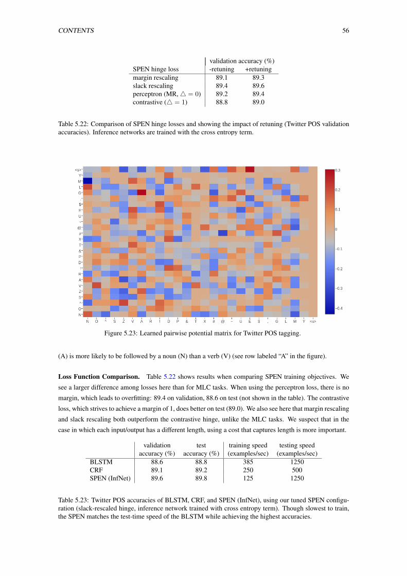
CONTENTS 56
validation accuracy (%)SPEN hinge loss -retuning +retuningmargin rescaling 89.1 89.3slack rescaling 89.4 89.6perceptron (MR,4 = 0) 89.2 89.4contrastive (4 = 1) 88.8 89.0
Table 5.22: Comparison of SPEN hinge losses and showing the impact of retuning (Twitter POS validationaccuracies). Inference networks are trained with the cross entropy term.
Figure 5.23: Learned pairwise potential matrix for Twitter POS tagging.
(A) is more likely to be followed by a noun (N) than a verb (V) (see row labeled “A” in the figure).
Loss Function Comparison. Table 5.22 shows results when comparing SPEN training objectives. We
see a larger difference among losses here than for MLC tasks. When using the perceptron loss, there is no
margin, which leads to overfitting: 89.4 on validation, 88.6 on test (not shown in the table). The contrastive
loss, which strives to achieve a margin of 1, does better on test (89.0). We also see here that margin rescaling
and slack rescaling both outperform the contrastive hinge, unlike the MLC tasks. We suspect that in the
case in which each input/output has a different length, using a cost that captures length is more important.
validation test training speed testing speedaccuracy (%) accuracy (%) (examples/sec) (examples/sec)
BLSTM 88.6 88.8 385 1250CRF 89.1 89.2 250 500SPEN (InfNet) 89.6 89.8 125 1250
Table 5.23: Twitter POS accuracies of BLSTM, CRF, and SPEN (InfNet), using our tuned SPEN configu-ration (slack-rescaled hinge, inference network trained with cross entropy term). Though slowest to train,the SPEN matches the test-time speed of the BLSTM while achieving the highest accuracies.
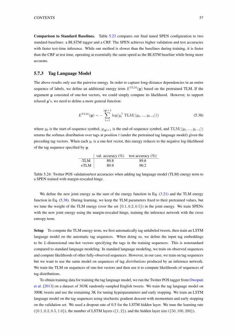
CONTENTS 57
Comparison to Standard Baselines. Table 5.23 compares our final tuned SPEN configuration to two
standard baselines: a BLSTM tagger and a CRF. The SPEN achieves higher validation and test accuracies
with faster test-time inference. While our method is slower than the baselines during training, it is faster
than the CRF at test time, operating at essentially the same speed as the BLSTM baseline while being more
accurate.
5.7.3 Tag Language Model
The above results only use the pairwise energy. In order to capture long-distance dependencies in an entire
sequence of labels, we define an additional energy term ETLM(y) based on the pretrained TLM. If the
argument y consisted of one-hot vectors, we could simply compute its likelihood. However, to support
relaxed y’s, we need to define a more general function:
ETLM(y) = −|y|+1∑t=1
log(y>t TLM(〈y0, ..., yt−1〉)) (5.38)
where y0 is the start-of-sequence symbol, y|y|+1 is the end-of-sequence symbol, and TLM(〈y0, ..., yt−1〉)returns the softmax distribution over tags at position t (under the pretrained tag language model) given the
preceding tag vectors. When each yt is a one-hot vector, this energy reduces to the negative log-likelihood
of the tag sequence specified by y.
val. accuracy (%) test accuracy (%)-TLM 89.8 89.6+TLM 89.9 90.2
Table 5.24: Twitter POS validation/test accuracies when adding tag language model (TLM) energy term toa SPEN trained with margin-rescaled hinge.
We define the new joint energy as the sum of the energy function in Eq. (3.21) and the TLM energy
function in Eq. (5.38). During learning, we keep the TLM parameters fixed to their pretrained values, but
we tune the weight of the TLM energy (over the set {0.1, 0.2, 0.5}) in the joint energy. We train SPENs
with the new joint energy using the margin-rescaled hinge, training the inference network with the cross
entropy term.
Setup To compute the TLM energy term, we first automatically tag unlabeled tweets, then train an LSTM
language model on the automatic tag sequences. When doing so, we define the input tag embeddings
to be L-dimensional one-hot vectors specifying the tags in the training sequences. This is nonstandard
compared to standard language modeling. In standard language modeling, we train on observed sequences
and compute likelihoods of other fully-observed sequences. However, in our case, we train on tag sequences
but we want to use the same model on sequences of tag distributions produced by an inference network.
We train the TLM on sequences of one-hot vectors and then use it to compute likelihoods of sequences of
tag distributions.
To obtain training data for training the tag language model, we run the Twitter POS tagger from Owoputi
et al. [2013] on a dataset of 303K randomly-sampled English tweets. We train the tag language model on
300K tweets and use the remaining 3K for tuning hyperparameters and early stopping. We train an LSTM
language model on the tag sequences using stochastic gradient descent with momentum and early stopping
on the validation set. We used a dropout rate of 0.5 for the LSTM hidden layer. We tune the learning rate
({0.1, 0.2, 0.5, 1.0}), the number of LSTM layers ({1, 2}), and the hidden layer size ({50, 100, 200}).
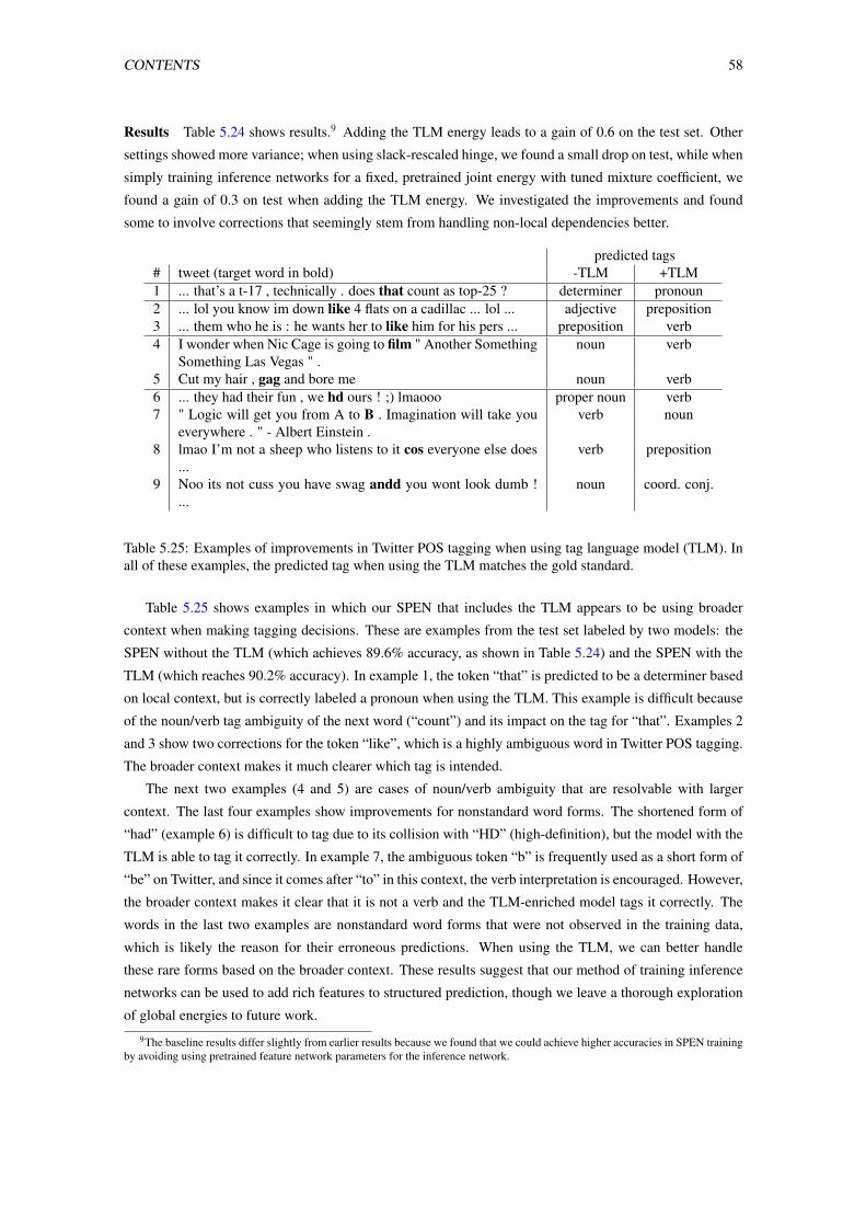
CONTENTS 58
Results Table 5.24 shows results.9 Adding the TLM energy leads to a gain of 0.6 on the test set. Other
settings showed more variance; when using slack-rescaled hinge, we found a small drop on test, while when
simply training inference networks for a fixed, pretrained joint energy with tuned mixture coefficient, we
found a gain of 0.3 on test when adding the TLM energy. We investigated the improvements and found
some to involve corrections that seemingly stem from handling non-local dependencies better.
predicted tags# tweet (target word in bold) -TLM +TLM1 ... that’s a t-17 , technically . does that count as top-25 ? determiner pronoun2 ... lol you know im down like 4 flats on a cadillac ... lol ... adjective preposition3 ... them who he is : he wants her to like him for his pers ... preposition verb4 I wonder when Nic Cage is going to film " Another Something
Something Las Vegas " .noun verb
5 Cut my hair , gag and bore me noun verb6 ... they had their fun , we hd ours ! ;) lmaooo proper noun verb7 " Logic will get you from A to B . Imagination will take you
everywhere . " - Albert Einstein .verb noun
8 lmao I’m not a sheep who listens to it cos everyone else does...
verb preposition
9 Noo its not cuss you have swag andd you wont look dumb !...
noun coord. conj.
Table 5.25: Examples of improvements in Twitter POS tagging when using tag language model (TLM). Inall of these examples, the predicted tag when using the TLM matches the gold standard.
Table 5.25 shows examples in which our SPEN that includes the TLM appears to be using broader
context when making tagging decisions. These are examples from the test set labeled by two models: the
SPEN without the TLM (which achieves 89.6% accuracy, as shown in Table 5.24) and the SPEN with the
TLM (which reaches 90.2% accuracy). In example 1, the token “that” is predicted to be a determiner based
on local context, but is correctly labeled a pronoun when using the TLM. This example is difficult because
of the noun/verb tag ambiguity of the next word (“count”) and its impact on the tag for “that”. Examples 2
and 3 show two corrections for the token “like”, which is a highly ambiguous word in Twitter POS tagging.
The broader context makes it much clearer which tag is intended.
The next two examples (4 and 5) are cases of noun/verb ambiguity that are resolvable with larger
context. The last four examples show improvements for nonstandard word forms. The shortened form of
“had” (example 6) is difficult to tag due to its collision with “HD” (high-definition), but the model with the
TLM is able to tag it correctly. In example 7, the ambiguous token “b” is frequently used as a short form of
“be” on Twitter, and since it comes after “to” in this context, the verb interpretation is encouraged. However,
the broader context makes it clear that it is not a verb and the TLM-enriched model tags it correctly. The
words in the last two examples are nonstandard word forms that were not observed in the training data,
which is likely the reason for their erroneous predictions. When using the TLM, we can better handle
these rare forms based on the broader context. These results suggest that our method of training inference
networks can be used to add rich features to structured prediction, though we leave a thorough exploration
of global energies to future work.
9The baseline results differ slightly from earlier results because we found that we could achieve higher accuracies in SPEN trainingby avoiding using pretrained feature network parameters for the inference network.

CONTENTS 59
5.8 CONCLUSIONS
We presented ways to jointly train structured energy functions and inference networks using large-margin
objectives. The energy function captures arbitrary dependencies among the labels, while theinference net-
works learns to capture the properties of the energy in an efficient manner, yielding fasttest-time inference.
Future work includes exploring the space of network architectures for inferencenetworks to balance accu-
racy and efficiency, experimenting with additional global terms in structuredenergy functions, and exploring
richer structured output spaces such as trees and sentences.
Joint Parameterizations for InferenceNetworks
In the previous chapter, we develop an efficient framework for energy-based models by training “inference
networks” to approximate structured inference instead of using gradient descent. However, their alternating
optimization approach suffers from instabilities during training, requiring additional loss terms and careful
hyperparameter tuning. In this paper, we contribute several strategies to stabilize and improve this joint
training of energy functions and inference networks for structured prediction. We design a compound ob-
jective to jointly train both cost-augmented and test-time inference networks along with the energy function.
We propose joint parameterizations for the inference networks that encourage them to capture complemen-
tary functionality during learning. We empirically validate our strategies on two sequence labeling tasks,
showing easier paths to strong performance than prior work, as well as further improvements with global
energy terms.
This chapter includes some material originally presented in Tu et al. [2020c].
6.1 Previous Pipeline
In the previous chapter, we jointly train the cost-augmented inference network and energy network, then do
fine-tuning of the cost-augmented inference network to make it more like a test-time inference network. In
our previous work, there are two steps in order to get the test-time inference network AΨ(x).
Step 1:
Θ, Φ = minΘ
maxΦ
∑〈xi,yi〉∈D
[4(FΦ(xi),yi)− EΘ(xi,FΦ(xi)) + EΘ(xi,yi)]+
Update Φ to yield output with low energy and high cost
Step 2: :
Ψ = argminΨ
EΘ(x,AΨ(x))
where AΨ is initialized by trained FΦ.
60
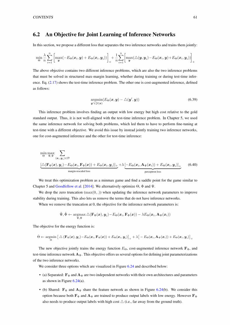
CONTENTS 61
6.2 An Objective for Joint Learning of Inference Networks
In this section, we propose a different loss that separates the two inference networks and trains them jointly:
minΘ
λ
n
n∑i=1
[maxy
(−EΘ(xi,y) + EΘ(xi,yi))
]+
+1
n
n∑i=1
[maxy
(4(y,yi)−EΘ(xi,y)+EΘ(xi,yi))
]+
The above objective contains two different inference problems, which are also the two inference problems
that must be solved in structured max-margin learning, whether during training or during test-time infer-
ence. Eq. (2.17) shows the test-time inference problem. The other one is cost-augmented inference, defined
as follows:
argminy′∈Y(x)
(EΘ(x,y)−4(y′,y)) (6.39)
This inference problem involves finding an output with low energy but high cost relative to the gold
standard output. Thus, it is not well-aligned with the test-time inference problem. In Chapter 5, we used
the same inference network for solving both problems, which led them to have to perform fine-tuning at
test-time with a different objective. We avoid this issue by instead jointly training two inference networks,
one for cost-augmented inference and the other for test-time inference:
minΘ
maxΦ,Ψ
∑〈xi,yi〉∈D
[4(FΦ(x),yi)−EΘ(xi,FΦ(x)) + EΘ(xi,yi)]+︸ ︷︷ ︸margin-rescaled loss
+λ [−EΘ(xi,AΨ(xi)) + EΘ(xi,yi)]+︸ ︷︷ ︸perceptron loss
(6.40)
We treat this optimization problem as a minmax game and find a saddle point for the game similar to
Chapter 5 and Goodfellow et al. [2014]. We alternatively optimize Θ, Φ and Ψ.
We drop the zero truncation (max(0, .)) when updating the inference network parameters to improve
stability during training. This also lets us remove the terms that do not have inference networks.
When we remove the truncation at 0, the objective for the inference network parameters is:
Ψ, Φ← argmaxΨ,Φ
4(FΦ(x),yi)−EΘ(xi,FΦ(x))− λEΘ(xi,AΨ(xi))
The objective for the energy function is:
Θ← argminΘ
[4 (FΦ(x),yi)−EΘ(xi,FΦ(x)) + EΘ(xi,yi)
]+
+ λ[− EΘ(xi,AΨ(xi)) + EΘ(xi,yi)
]+
The new objective jointly trains the energy function EΘ, cost-augmented inference network FΦ, and
test-time inference network AΨ. This objective offers us several options for defining joint parameterizations
of the two inference networks.
We consider three options which are visualized in Figure 6.24 and described below:
• (a) Separated: FΦ and AΨ are two independent networks with their own architectures and parameters
as shown in Figure 6.24(a).
• (b) Shared: FΦ and AΨ share the feature network as shown in Figure 6.24(b). We consider this
option because both FΦ and AΨ are trained to produce output labels with low energy. However FΦ
also needs to produce output labels with high cost4 (i.e., far away from the ground truth).
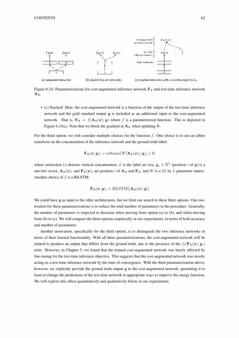
CONTENTS 62
Figure 6.24: Parameterizations for cost-augmented inference network FΦ and test-time inference networkAΨ.
• (c) Stacked: Here, the cost-augmented network is a function of the output of the test-time inference
network and the gold standard output y is included as an additional input to the cost-augmented
network. That is, FΦ = f(AΨ(x),y) where f is a parameterized function. This is depicted in
Figure 6.24(c). Note that we block the gradient at AΨ when updating Ψ.
For the third option, we will consider multiple choices for the function f . One choice is to use an affine
transform on the concatenation of the inference network and the ground truth label:
FΦ(x,y)i = softmax(W [AΨ(x)i;yi] + b)
where semicolon (;) denotes vertical concatenation, L is the label set size, yi ∈ RL (position i of y) is a
one-hot vector, AΨ(x)i and FΦ(x)i are position i of AΨ and FΦ, and W is a 2L by L parameter matrix.
Another choice of f is a BiLSTM:
FΦ(x,y)i = BiLSTM([AΨ(x);y])
We could have y as input to the other architectures, but we limit our search to these three options. One mo-
tivation for these parameterizations is to reduce the total number of parameters in the procedure. Generally,
the number of parameters is expected to decrease when moving from option (a) to (b), and when moving
from (b) to (c). We will compare the three options empirically in our experiments, in terms of both accuracy
and number of parameters.
Another motivation, specifically for the third option, is to distinguish the two inference networks in
terms of their learned functionality. With all three parameterizations, the cost-augmented network will be
trained to produce an output that differs from the ground truth, due to the presence of the 4(FΦ(x),yi)
term. However, in Chapter 5, we found that the trained cost-augmented network was barely affected by
fine-tuning for the test-time inference objective. This suggests that the cost-augmented network was mostly
acting as a test-time inference network by the time of convergence. With the third parameterization above,
however, we explicitly provide the ground truth output y to the cost-augmented network, permitting it to
learn to change the predictions of the test-time network in appropriate ways to improve the energy function.
We will explore this effect quantitatively and qualitatively below in our experiments.
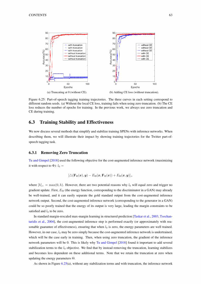
CONTENTS 63
(a) Truncating at 0 (without CE). (b) Adding CE loss (without truncation).
Figure 6.25: Part-of-speech tagging training trajectories. The three curves in each setting correspond todifferent random seeds. (a) Without the local CE loss, training fails when using zero truncation. (b) The CEloss reduces the number of epochs for training. In the previous work, we always use zero truncation andCE during training.
6.3 Training Stability and Effectiveness
We now discuss several methods that simplify and stabilize training SPENs with inference networks. When
describing them, we will illustrate their impact by showing training trajectories for the Twitter part-of-
speech tagging task.
6.3.1 Removing Zero Truncation
Tu and Gimpel [2018] used the following objective for the cost-augmented inference network (maximizing
it with respect to Φ): l0 =
[4(FΦ(x),y)− EΘ(x,FΦ(x)) + EΘ(x,y)]+
where [h]+ = max(0, h). However, there are two potential reasons why l0 will equal zero and trigger no
gradient update. First, EΘ (the energy function, corresponding to the discriminator in a GAN) may already
be well-trained, and it can easily separate the gold standard output from the cost-augmented inference
network output. Second, the cost-augmented inference network (corresponding to the generator in a GAN)
could be so poorly trained that the energy of its output is very large, leading the margin constraints to be
satisfied and l0 to be zero.
In standard margin-rescaled max-margin learning in structured prediction [Taskar et al., 2003, Tsochan-
taridis et al., 2004], the cost-augmented inference step is performed exactly (or approximately with rea-
sonable guarantee of effectiveness), ensuring that when l0 is zero, the energy parameters are well trained.
However, in our case, l0 may be zero simply because the cost-augmented inference network is undertrained,
which will be the case early in training. Then, when using zero truncation, the gradient of the inference
network parameters will be 0. This is likely why Tu and Gimpel [2018] found it important to add several
stabilization terms to the l0 objective. We find that by instead removing the truncation, learning stabilizes
and becomes less dependent on these additional terms. Note that we retain the truncation at zero when
updating the energy parameters Θ.
As shown in Figure 6.25(a), without any stabilization terms and with truncation, the inference network
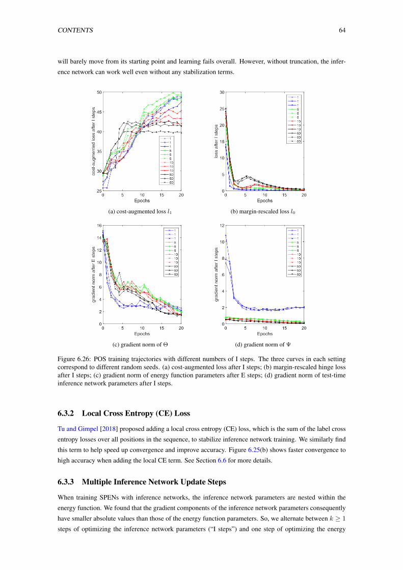
CONTENTS 64
will barely move from its starting point and learning fails overall. However, without truncation, the infer-
ence network can work well even without any stabilization terms.
(a) cost-augmented loss l1 (b) margin-rescaled loss l0
(c) gradient norm of Θ (d) gradient norm of Ψ
Figure 6.26: POS training trajectories with different numbers of I steps. The three curves in each settingcorrespond to different random seeds. (a) cost-augmented loss after I steps; (b) margin-rescaled hinge lossafter I steps; (c) gradient norm of energy function parameters after E steps; (d) gradient norm of test-timeinference network parameters after I steps.
6.3.2 Local Cross Entropy (CE) Loss
Tu and Gimpel [2018] proposed adding a local cross entropy (CE) loss, which is the sum of the label cross
entropy losses over all positions in the sequence, to stabilize inference network training. We similarly find
this term to help speed up convergence and improve accuracy. Figure 6.25(b) shows faster convergence to
high accuracy when adding the local CE term. See Section 6.6 for more details.
6.3.3 Multiple Inference Network Update Steps
When training SPENs with inference networks, the inference network parameters are nested within the
energy function. We found that the gradient components of the inference network parameters consequently
have smaller absolute values than those of the energy function parameters. So, we alternate between k ≥ 1
steps of optimizing the inference network parameters (“I steps”) and one step of optimizing the energy
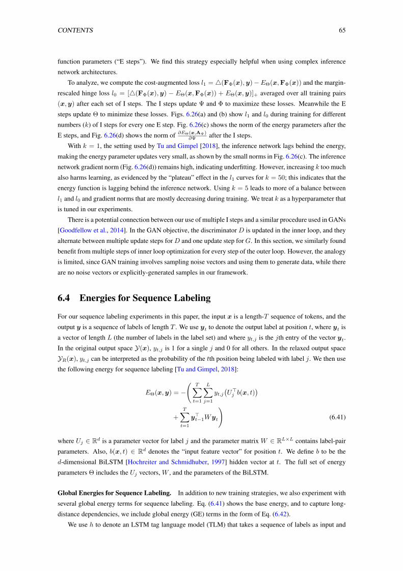
CONTENTS 65
function parameters (“E steps”). We find this strategy especially helpful when using complex inference
network architectures.
To analyze, we compute the cost-augmented loss l1 = 4(FΦ(x),y)−EΘ(x,FΦ(x)) and the margin-
rescaled hinge loss l0 = [4(FΦ(x),y) − EΘ(x,FΦ(x)) + EΘ(x,y)]+ averaged over all training pairs
(x,y) after each set of I steps. The I steps update Ψ and Φ to maximize these losses. Meanwhile the E
steps update Θ to minimize these losses. Figs. 6.26(a) and (b) show l1 and l0 during training for different
numbers (k) of I steps for every one E step. Fig. 6.26(c) shows the norm of the energy parameters after the
E steps, and Fig. 6.26(d) shows the norm of ∂EΘ(x,AΨ)∂Ψ after the I steps.
With k = 1, the setting used by Tu and Gimpel [2018], the inference network lags behind the energy,
making the energy parameter updates very small, as shown by the small norms in Fig. 6.26(c). The inference
network gradient norm (Fig. 6.26(d)) remains high, indicating underfitting. However, increasing k too much
also harms learning, as evidenced by the “plateau” effect in the l1 curves for k = 50; this indicates that the
energy function is lagging behind the inference network. Using k = 5 leads to more of a balance between
l1 and l0 and gradient norms that are mostly decreasing during training. We treat k as a hyperparameter that
is tuned in our experiments.
There is a potential connection between our use of multiple I steps and a similar procedure used in GANs
[Goodfellow et al., 2014]. In the GAN objective, the discriminator D is updated in the inner loop, and they
alternate between multiple update steps forD and one update step forG. In this section, we similarly found
benefit from multiple steps of inner loop optimization for every step of the outer loop. However, the analogy
is limited, since GAN training involves sampling noise vectors and using them to generate data, while there
are no noise vectors or explicitly-generated samples in our framework.
6.4 Energies for Sequence Labeling
For our sequence labeling experiments in this paper, the input x is a length-T sequence of tokens, and the
output y is a sequence of labels of length T . We use yt to denote the output label at position t, where yt is
a vector of length L (the number of labels in the label set) and where yt,j is the jth entry of the vector yt.
In the original output space Y(x), yt,j is 1 for a single j and 0 for all others. In the relaxed output space
YR(x), yt,j can be interpreted as the probability of the tth position being labeled with label j. We then use
the following energy for sequence labeling [Tu and Gimpel, 2018]:
EΘ(x,y) = −
(T∑t=1
L∑j=1
yt,j(U>j b(x, t)
)+
T∑t=1
y>t−1Wyt
)(6.41)
where Uj ∈ Rd is a parameter vector for label j and the parameter matrix W ∈ RL×L contains label-pair
parameters. Also, b(x, t) ∈ Rd denotes the “input feature vector” for position t. We define b to be the
d-dimensional BiLSTM [Hochreiter and Schmidhuber, 1997] hidden vector at t. The full set of energy
parameters Θ includes the Uj vectors, W , and the parameters of the BiLSTM.
Global Energies for Sequence Labeling. In addition to new training strategies, we also experiment with
several global energy terms for sequence labeling. Eq. (6.41) shows the base energy, and to capture long-
distance dependencies, we include global energy (GE) terms in the form of Eq. (6.42).
We use h to denote an LSTM tag language model (TLM) that takes a sequence of labels as input and
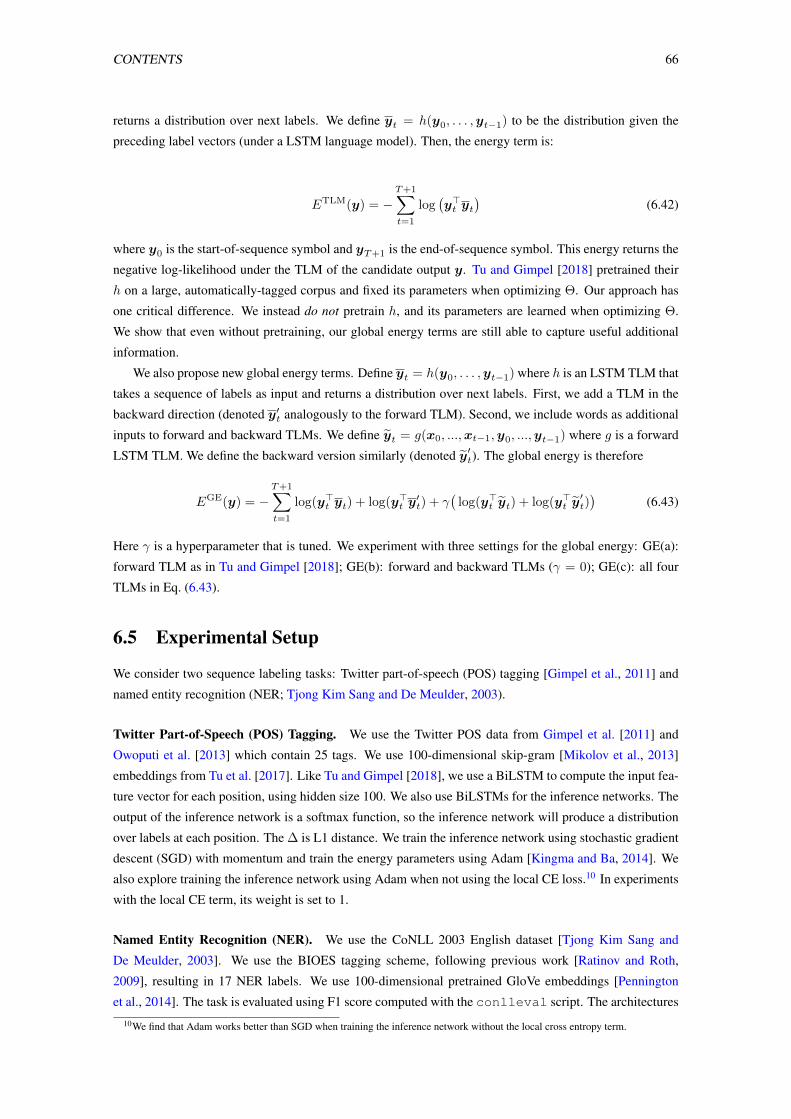
CONTENTS 66
returns a distribution over next labels. We define yt = h(y0, . . . ,yt−1) to be the distribution given the
preceding label vectors (under a LSTM language model). Then, the energy term is:
ETLM(y) = −T+1∑t=1
log(y>t yt
)(6.42)
where y0 is the start-of-sequence symbol and yT+1 is the end-of-sequence symbol. This energy returns the
negative log-likelihood under the TLM of the candidate output y. Tu and Gimpel [2018] pretrained their
h on a large, automatically-tagged corpus and fixed its parameters when optimizing Θ. Our approach has
one critical difference. We instead do not pretrain h, and its parameters are learned when optimizing Θ.
We show that even without pretraining, our global energy terms are still able to capture useful additional
information.
We also propose new global energy terms. Define yt = h(y0, . . . ,yt−1) where h is an LSTM TLM that
takes a sequence of labels as input and returns a distribution over next labels. First, we add a TLM in the
backward direction (denoted y′t analogously to the forward TLM). Second, we include words as additional
inputs to forward and backward TLMs. We define yt = g(x0, ...,xt−1,y0, ...,yt−1) where g is a forward
LSTM TLM. We define the backward version similarly (denoted y′t). The global energy is therefore
EGE(y) = −T+1∑t=1
log(y>t yt) + log(y>t y′t) + γ
(log(y>t yt) + log(y>t y
′t))
(6.43)
Here γ is a hyperparameter that is tuned. We experiment with three settings for the global energy: GE(a):
forward TLM as in Tu and Gimpel [2018]; GE(b): forward and backward TLMs (γ = 0); GE(c): all four
TLMs in Eq. (6.43).
6.5 Experimental Setup
We consider two sequence labeling tasks: Twitter part-of-speech (POS) tagging [Gimpel et al., 2011] and
named entity recognition (NER; Tjong Kim Sang and De Meulder, 2003).
Twitter Part-of-Speech (POS) Tagging. We use the Twitter POS data from Gimpel et al. [2011] and
Owoputi et al. [2013] which contain 25 tags. We use 100-dimensional skip-gram [Mikolov et al., 2013]
embeddings from Tu et al. [2017]. Like Tu and Gimpel [2018], we use a BiLSTM to compute the input fea-
ture vector for each position, using hidden size 100. We also use BiLSTMs for the inference networks. The
output of the inference network is a softmax function, so the inference network will produce a distribution
over labels at each position. The ∆ is L1 distance. We train the inference network using stochastic gradient
descent (SGD) with momentum and train the energy parameters using Adam [Kingma and Ba, 2014]. We
also explore training the inference network using Adam when not using the local CE loss.10 In experiments
with the local CE term, its weight is set to 1.
Named Entity Recognition (NER). We use the CoNLL 2003 English dataset [Tjong Kim Sang and
De Meulder, 2003]. We use the BIOES tagging scheme, following previous work [Ratinov and Roth,
2009], resulting in 17 NER labels. We use 100-dimensional pretrained GloVe embeddings [Pennington
et al., 2014]. The task is evaluated using F1 score computed with the conlleval script. The architectures
10We find that Adam works better than SGD when training the inference network without the local cross entropy term.
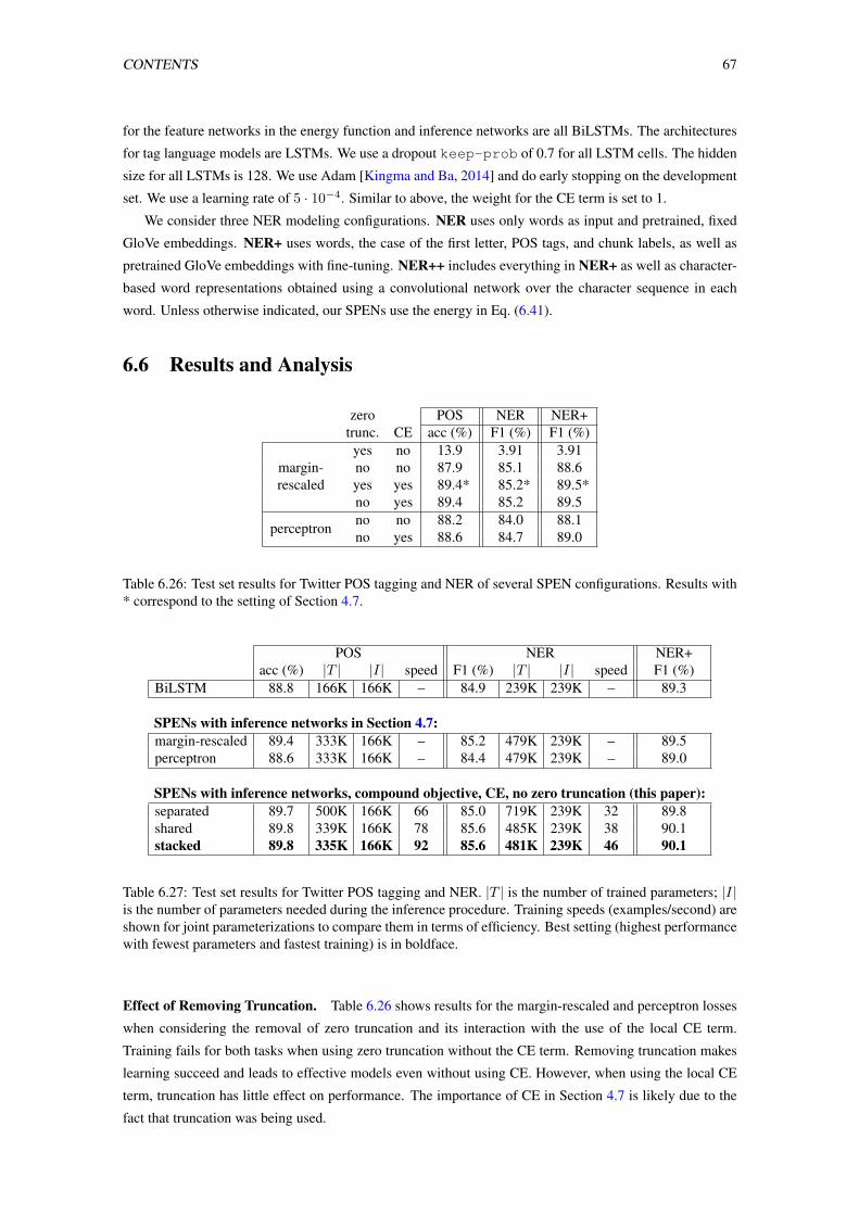
CONTENTS 67
for the feature networks in the energy function and inference networks are all BiLSTMs. The architectures
for tag language models are LSTMs. We use a dropout keep-prob of 0.7 for all LSTM cells. The hidden
size for all LSTMs is 128. We use Adam [Kingma and Ba, 2014] and do early stopping on the development
set. We use a learning rate of 5 · 10−4. Similar to above, the weight for the CE term is set to 1.
We consider three NER modeling configurations. NER uses only words as input and pretrained, fixed
GloVe embeddings. NER+ uses words, the case of the first letter, POS tags, and chunk labels, as well as
pretrained GloVe embeddings with fine-tuning. NER++ includes everything in NER+ as well as character-
based word representations obtained using a convolutional network over the character sequence in each
word. Unless otherwise indicated, our SPENs use the energy in Eq. (6.41).
6.6 Results and Analysis
zero POS NER NER+trunc. CE acc (%) F1 (%) F1 (%)yes no 13.9 3.91 3.91
margin- no no 87.9 85.1 88.6rescaled yes yes 89.4* 85.2* 89.5*
no yes 89.4 85.2 89.5
perceptron no no 88.2 84.0 88.1no yes 88.6 84.7 89.0
Table 6.26: Test set results for Twitter POS tagging and NER of several SPEN configurations. Results with* correspond to the setting of Section 4.7.
POS NER NER+acc (%) |T | |I| speed F1 (%) |T | |I| speed F1 (%)
BiLSTM 88.8 166K 166K – 84.9 239K 239K – 89.3
SPENs with inference networks in Section 4.7:margin-rescaled 89.4 333K 166K – 85.2 479K 239K – 89.5perceptron 88.6 333K 166K – 84.4 479K 239K – 89.0
SPENs with inference networks, compound objective, CE, no zero truncation (this paper):separated 89.7 500K 166K 66 85.0 719K 239K 32 89.8shared 89.8 339K 166K 78 85.6 485K 239K 38 90.1stacked 89.8 335K 166K 92 85.6 481K 239K 46 90.1
Table 6.27: Test set results for Twitter POS tagging and NER. |T | is the number of trained parameters; |I|is the number of parameters needed during the inference procedure. Training speeds (examples/second) areshown for joint parameterizations to compare them in terms of efficiency. Best setting (highest performancewith fewest parameters and fastest training) is in boldface.
Effect of Removing Truncation. Table 6.26 shows results for the margin-rescaled and perceptron losses
when considering the removal of zero truncation and its interaction with the use of the local CE term.
Training fails for both tasks when using zero truncation without the CE term. Removing truncation makes
learning succeed and leads to effective models even without using CE. However, when using the local CE
term, truncation has little effect on performance. The importance of CE in Section 4.7 is likely due to the
fact that truncation was being used.
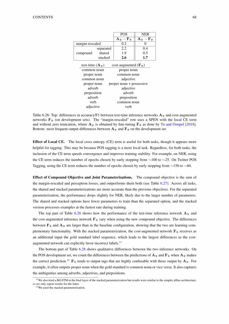
CONTENTS 68
POS NERAΨ − FΦ AΨ − FΦ
margin-rescaled 0.2 0separated 2.2 0.4
compound shared 1.9 0.5stacked 2.6 1.7
test-time (AΨ) cost-augmented (FΦ)common noun proper nounproper noun common noun
common noun adjectiveproper noun proper noun + possessive
adverb adjectivepreposition adverb
adverb prepositionverb common noun
adjective verb
Table 6.28: Top: differences in accuracy/F1 between test-time inference networks AΨ and cost-augmentednetworks FΦ (on development sets). The “margin-rescaled” row uses a SPEN with the local CE termand without zero truncation, where AΨ is obtained by fine-tuning FΦ as done by Tu and Gimpel [2018].Bottom: most frequent output differences between AΨ and FΦ on the development set.
Effect of Local CE. The local cross entropy (CE) term is useful for both tasks, though it appears more
helpful for tagging. This may be because POS tagging is a more local task. Regardless, for both tasks, the
inclusion of the CE term speeds convergence and improves training stability. For example, on NER, using
the CE term reduces the number of epochs chosen by early stopping from ∼100 to ∼25. On Twitter POS
Tagging, using the CE term reduces the number of epochs chosen by early stopping from ∼150 to ∼60.
Effect of Compound Objective and Joint Parameterizations. The compound objective is the sum of
the margin-rescaled and perceptron losses, and outperforms them both (see Table 6.27). Across all tasks,
the shared and stacked parameterizations are more accurate than the previous objectives. For the separated
parameterization, the performance drops slightly for NER, likely due to the larger number of parameters.
The shared and stacked options have fewer parameters to train than the separated option, and the stacked
version processes examples at the fastest rate during training.
The top part of Table 6.28 shows how the performance of the test-time inference network AΨ and
the cost-augmented inference network FΦ vary when using the new compound objective. The differences
between FΦ and AΨ are larger than in the baseline configuration, showing that the two are learning com-
plementary functionality. With the stacked parameterization, the cost-augmented network FΦ receives as
an additional input the gold standard label sequence, which leads to the largest differences as the cost-
augmented network can explicitly favor incorrect labels.11
The bottom part of Table 6.28 shows qualitative differences between the two inference networks. On
the POS development set, we count the differences between the predictions of AΨ and FΦ when AΨ makes
the correct prediction.12 FΦ tends to output tags that are highly confusable with those output by AΨ. For
example, it often outputs proper noun when the gold standard is common noun or vice versa. It also captures
the ambiguities among adverbs, adjectives, and prepositions.
11We also tried a BiLSTM in the final layer of the stacked parameterization but results were similar to the simpler affine architecture,so we only report results for the latter.
12We used the stacked parameterization.
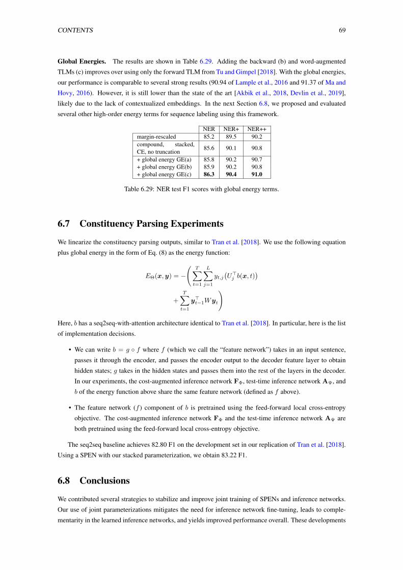
CONTENTS 69
Global Energies. The results are shown in Table 6.29. Adding the backward (b) and word-augmented
TLMs (c) improves over using only the forward TLM from Tu and Gimpel [2018]. With the global energies,
our performance is comparable to several strong results (90.94 of Lample et al., 2016 and 91.37 of Ma and
Hovy, 2016). However, it is still lower than the state of the art [Akbik et al., 2018, Devlin et al., 2019],
likely due to the lack of contextualized embeddings. In the next Section 6.8, we proposed and evaluated
several other high-order energy terms for sequence labeling using this framework.
NER NER+ NER++margin-rescaled 85.2 89.5 90.2compound, stacked,CE, no truncation
85.6 90.1 90.8
+ global energy GE(a) 85.8 90.2 90.7+ global energy GE(b) 85.9 90.2 90.8+ global energy GE(c) 86.3 90.4 91.0
Table 6.29: NER test F1 scores with global energy terms.
6.7 Constituency Parsing Experiments
We linearize the constituency parsing outputs, similar to Tran et al. [2018]. We use the following equation
plus global energy in the form of Eq. (8) as the energy function:
EΘ(x,y) = −
(T∑t=1
L∑j=1
yt,j(U>j b(x, t)
)+
T∑t=1
y>t−1Wyt
)
Here, b has a seq2seq-with-attention architecture identical to Tran et al. [2018]. In particular, here is the list
of implementation decisions.
• We can write b = g ◦ f where f (which we call the “feature network”) takes in an input sentence,
passes it through the encoder, and passes the encoder output to the decoder feature layer to obtain
hidden states; g takes in the hidden states and passes them into the rest of the layers in the decoder.
In our experiments, the cost-augmented inference network FΦ, test-time inference network AΨ, and
b of the energy function above share the same feature network (defined as f above).
• The feature network (f ) component of b is pretrained using the feed-forward local cross-entropy
objective. The cost-augmented inference network FΦ and the test-time inference network AΨ are
both pretrained using the feed-forward local cross-entropy objective.
The seq2seq baseline achieves 82.80 F1 on the development set in our replication of Tran et al. [2018].
Using a SPEN with our stacked parameterization, we obtain 83.22 F1.
6.8 Conclusions
We contributed several strategies to stabilize and improve joint training of SPENs and inference networks.
Our use of joint parameterizations mitigates the need for inference network fine-tuning, leads to comple-
mentarity in the learned inference networks, and yields improved performance overall. These developments

CONTENTS 70
offer promise for SPENs to be more easily applied to a broad range of NLP tasks. Future work will ex-
plore other structured prediction tasks, such as parsing and generation. We have taken initial steps in this
direction, considering constituency parsing with the sequence-to-sequence model of Tran et al. [2018]. Pre-
liminary experiments are positive,13 but significant challenges remain, specifically in defining appropriate
inference network architectures to enable efficient learning.
13On NXT Switchboard [Calhoun et al., 2010], the baseline achieves 82.80 F1 on the development set and the SPEN (stackedparameterization) achieves 83.22. More details are in the appendix.
Exploration of Arbitrary-OrderSequence Labeling
A major challenge with CRFs is the complexity of training and inference, which are quadratic in the number
of output labels for first order models and grow exponentially when higher order dependencies are consid-
ered. This explains why the most common type of CRF used in practice is a first order model, also referred
to as a “linear chain” CRF.
In the previous chapter, we propose a framework that can Jointly train of energy functions and inference
networks. In this section, we leverage the frameworks to explore high-order energy functions for sequence
labeling. Naively instantiating high-order energy terms can lead to a very large number of parameters to
learn, so we instead develop concise neural parameterizations for high-order terms. In particular, we draw
from vectorized Kronecker products, convolutional networks, recurrent networks, and self-attention.
This chapter includes some material originally presented in Tu et al. [2020b].
7.1 Introduction
Conditional random fields (CRFs; Lafferty et al., 2001) have been shown to perform well in various se-
quence labeling tasks. Recent work uses rich neural network architectures to define the “unary” potentials,
i.e., terms that only consider a single position’s label at a time [Collobert et al., 2011, Lample et al., 2016,
Ma and Hovy, 2016, Strubell et al., 2018]. However, “binary” potentials, which consider pairs of adjacent
labels, are usually quite simple and may consist solely of a parameter or parameter vector for each unique
label transition. Models with unary and binary potentials are generally referred to as “first order” models.
A major challenge with CRFs is the complexity of training and inference, which are quadratic in the
number of output labels for first order models and grow exponentially when higher order dependencies are
considered. This explains why the most common type of CRF used in practice is a first order model, also
referred to as a “linear chain” CRF.
One promising alternative to CRFs is structured prediction energy networks (SPENs; Belanger and Mc-
Callum, 2016), which use deep neural networks to parameterize arbitrary potential functions for structured
prediction. While SPENs also pose challenges for learning and inference, in the previous chapters, we
proposed a way to train SPENs jointly with “inference networks”, neural networks trained to approximate
structured argmax inference.
In this paper, we leverage the frameworks of SPENs and inference networks to explore high-order
energy functions for sequence labeling. Naively instantiating high-order energy terms can lead to a very
large number of parameters to learn, so we instead develop concise neural parameterizations for high-
order terms. In particular, we draw from vectorized Kronecker products, convolutional networks, recurrent
networks, and self-attention. We also consider “skip-chain” connections [Sutton and McCallum, 2004] with
71
CONTENTS 72
various skip distances and ways of reducing their total parameter count for increased learnability.
Our experimental results on four sequence labeling tasks show that a range of high-order energy func-
tions can yield performance improvements. While the optimal energy function varies by task, we find strong
performance from skip-chain terms with short skip distances, convolutional networks with filters that con-
sider label trigrams, and recurrent networks and self-attention networks that consider large subsequences of
labels.
We also demonstrate that modeling high-order dependencies can lead to significant performance im-
provements in the setting of noisy training and test sets. Visualizations of the high-order energies show
various methods capture intuitive structured dependencies among output labels.
Throughout, we use inference networks that share the same architecture as unstructured classifiers for
sequence labeling, so test time inference speeds are unchanged between local models and our method.
Enlarging the inference network architecture by adding one layer leads consistently to better results, rivaling
or improving over a BiLSTM-CRF baseline, suggesting that training efficient inference networks with high-
order energy terms can make up for errors arising from approximate inference. While we focus on sequence
labeling in this paper, our results show the potential of developing high-order structured models for other
NLP tasks in the future.
7.2 Energy Functions
Considering sequence labeling tasks, the input x is a length-T sequence of tokens where xt denotes the
token at position t. The output y is a sequence of labels also of length T . We use yt to denote the output
label at position t, where yt is a vector of length L (the number of labels in the label set) and where yt,j is
the jth entry of the vector yt. In the original output space Y(x), yt,j is 1 for a single j and 0 for all others.
In the relaxed output space YR(x), yt,j can be interpreted as the probability of the tth position being labeled
with label j. We use the following energy:
EΘ(x,y) = −
(T∑t=1
L∑j=1
yt,j(U>j b(x, t)
)+ EW (y)
)(7.44)
where Uj ∈ Rd is a parameter vector for label j and EW (y) is a structured energy term parameterized by
parameters W . In a linear chain CRF, W is a transition matrix for scoring two adjacent labels. Different
instantiations of EW will be detailed in the sections below. Also, b(x, t) ∈ Rd denotes the “input feature
vector” for position t. We define it to be the d-dimensional BiLSTM [Hochreiter and Schmidhuber, 1997]
hidden vector at t. The full set of energy parameters Θ includes the Uj vectors, W , and the parameters of
the BiLSTM.
Table 7.30 shows the training and test-time inference requirements of our method compared to previous
methods. For different formulations of the energy function, the inference network architecture is the same
(e.g., BiLSTM). So the inference complexity is the same as the standard neural approaches that do not use
structured prediction, which is linear in the label set size. However, even for the first order model (linear-
chain CRF), the time complexity is quadratic in the label set size. The time complexity of higher-order
CRFs grows exponentially with the order.
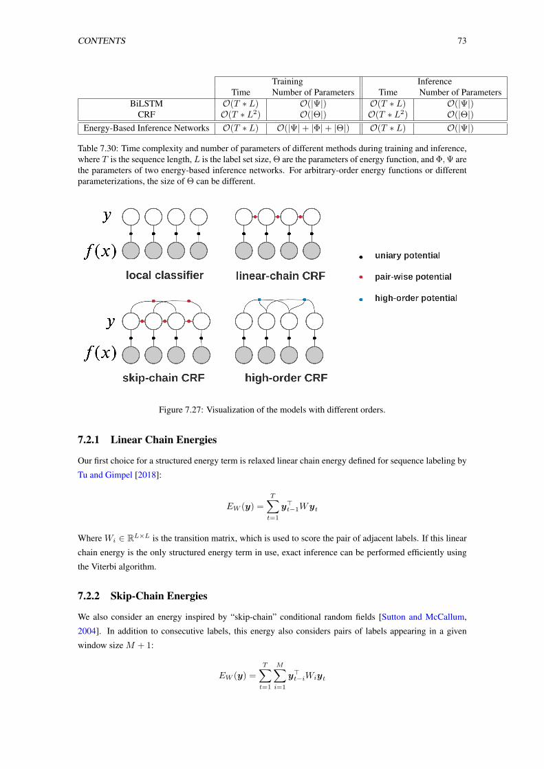
CONTENTS 73
Training InferenceTime Number of Parameters Time Number of Parameters
BiLSTM O(T ∗ L) O(|Ψ|) O(T ∗ L) O(|Ψ|)CRF O(T ∗ L2) O(|Θ|) O(T ∗ L2) O(|Θ|)
Energy-Based Inference Networks O(T ∗ L) O(|Ψ|+ |Φ|+ |Θ|) O(T ∗ L) O(|Ψ|)
Table 7.30: Time complexity and number of parameters of different methods during training and inference,where T is the sequence length, L is the label set size, Θ are the parameters of energy function, and Φ,Ψ arethe parameters of two energy-based inference networks. For arbitrary-order energy functions or differentparameterizations, the size of Θ can be different.
Figure 7.27: Visualization of the models with different orders.
7.2.1 Linear Chain Energies
Our first choice for a structured energy term is relaxed linear chain energy defined for sequence labeling by
Tu and Gimpel [2018]:
EW (y) =
T∑t=1
y>t−1Wyt
Where Wi ∈ RL×L is the transition matrix, which is used to score the pair of adjacent labels. If this linear
chain energy is the only structured energy term in use, exact inference can be performed efficiently using
the Viterbi algorithm.
7.2.2 Skip-Chain Energies
We also consider an energy inspired by “skip-chain” conditional random fields [Sutton and McCallum,
2004]. In addition to consecutive labels, this energy also considers pairs of labels appearing in a given
window size M + 1:
EW (y) =
T∑t=1
M∑i=1
y>t−iWiyt
CONTENTS 74
where each Wi ∈ RL×L and the max window size M is a hyperparameter. While linear chain energies
allow efficient exact inference, using skip-chain energies causes exact inference to require time exponential
in the size of M .
7.2.3 High-Order Energies
We also consider M th-order energy terms. We use the function F to score the M + 1 consecutive labels
yt−M , . . . ,yt, then sum over positions:
EW (y) =
T∑t=M
F (yt−M , . . . ,yt) (7.45)
We consider several different ways to define the function F , detailed below.
Vectorized Kronecker Product (VKP): A naive way to parameterize a high-order energy term would
involve using a parameter tensor W ∈ RLM+1
with an entry for each possible label sequence of length
M+1. To avoid this exponentially-large number of parameters, we define a more efficient parameterization
as follows. We first define a label embedding lookup table ∈ RL×nl and denote the embedding for label j
by ej . We consider M = 2 as an example. Then, for a tensor W ∈ RL×L×L, its value Wi,j,k at indices
(i, j, k) is calculated as
v>LayerNorm([ei; ej ; ek] + MLP([ei; ej ; ek]))
where v ∈ R(M+1)nl is a parameter vector and ‘;′ denotes vector concatenation. MLP expects and returns
vectors of dimension (M + 1)× nl and is parameterized as a multilayer perceptron. Then, the energy is
computed:
F (yt−M , . . . ,yt) = VKP(yt−M , . . . ,yt−1)Wyt
where W is reshaped as ∈ RLM×L. The operator VKP is somewhat similar to the Kronecker product of
the k vectors v1, . . . ,vk14. However it will return a vector, not a tensor:
VKP(v1, . . . ,vk) =v1 k = 1
vec(v1v>2 ) k = 2
vec(VKP(v1, . . . ,vk−1)v>k ) k > 2
Where vec is the operation that vectorizes a tensor into a (column) vector.
CNN: Convolutional neural networks (CNN) are frequently used in NLP to extract features based on
words or characters [Collobert et al., 2011, Kim, 2014]. We apply CNN filters over the sequence of M + 1
consecutive labels. The F function is computed as follows:
F (yt−M , . . . ,yt) =∑n
fn(yt−M , . . . ,yt)
fn(yt−M , . . . ,yt) = g(Wn[yt−M ; ...;yt] + bn)
14There are some work [Lei et al., 2014, Srikumar and Manning, 2014, Yu et al., 2016] that use Kronecker product for higher orderfeature combinations with low-rank tensors. Here we use this form to express the computation when scoring the consecutive labels.
CONTENTS 75
where g is a ReLU nonlinearity and the vector Wn ∈ RL(M+1) and scalar bn ∈ R are the parameters for
filter n. The filter size of all filters is the same as the window size, namely, M + 1. The F function sums
over all CNN filters. When viewing this high-order energy as a CNN, we can think of the summation in
Eq. 7.45 as corresponding to sum pooling over time of the feature map outputs.
Tag Language Model (TLM): Tu and Gimpel [2018] defined an energy term based on a pretrained “tag
language model”, which computes the probability of an entire sequence of labels. We also use a TLM,
scoring a sequence of M + 1 consecutive labels in a way similar to Tu and Gimpel [2018]; however, the
parameters of the TLM are trained in our setting:
F (yt−M , . . . ,yt) =
−t∑
t′=t−M+1
y>t′ log(TLM(〈yt−M , ...,yt′−1〉))
where TLM(〈yt−M , ..., yt′−1〉) returns the softmax distribution over tags at position t′ (under the tag lan-
guage model) given the preceding tag vectors. When each yt′ is a one-hot vector, this energy reduces to the
negative log-likelihood of the tag sequence specified by yt−M , . . . ,yt.
Self-Attention (S-Att): We adopt the multi-head self-attention formulation from Vaswani et al. [2017].
Given a matrix of the M + 1 consecutive labels Q = K = V = [yt−M ; . . . ;yt] ∈ R(M+1)×L:
H = attention(Q,K, V )
F (yt−M , . . . ,yt) =∑
H
where attention is the general attention mechanism: the weighted sum of the value vectors V using query
vectors Q and key vectors K [Vaswani et al., 2017]. The energy on the M + 1 consecutive labels is defined
as the sum of entries in the feature map H ∈ RL×(M+1) after the self-attention transformation.
7.2.4 Fully-Connected Energies
We can simulate a “fully-connected” energy function by setting a very large value for M in the skip-chain
energy (Section 7.2.2). For efficiency and learnability, we use a low-rank parameterization for the many
translation matrices Wi that will result from increasing M . We first define a matrix S ∈ RL×d that all Wi
will use. Each i has a learned parameter matrix Di ∈ RL×d and together S and Di are used to compute
Wi:
Wi = SD>i
where d is a tunable hyperparameter that affects the number of learnable parameters.
7.3 Related Work
Linear chain CRFs [Lafferty et al., 2001], which consider dependencies between at most two adjacent labels
or segments, are commonly used in practice [Sarawagi and Cohen, 2005, Lample et al., 2016, Ma and Hovy,
2016].
CONTENTS 76
There have been several efforts in developing efficient algorithms for handling higher-order CRFs. Qian
et al. [2009] developed an efficient decoding algorithm under the assumption that all high-order features
have non-negative weights. Some work has shown that high-order CRFs can be handled relatively effi-
ciently if particular patterns of sparsity are assumed [Ye et al., 2009, Cuong et al., 2014]. Mueller et al.
[2013] proposed an approximate CRF using coarse-to-fine decoding and early updating. Loopy belief
propagation [Murphy et al., 1999] has been used for approximate inference in high-order CRFs, such as
skip-chain CRFs [Sutton and McCallum, 2004], which form the inspiration for one category of energy
function in this paper. .
CRFs are typically trained by maximizing conditional log-likelihood. Even assuming that the graph
structure underlying the CRF admits tractable inference, it is still time-consuming to compute the partition
function. Margin-based methods have been proposed [Taskar et al., 2003, Tsochantaridis et al., 2004] to
avoid the summation over all possible outputs. Similar losses are used when training SPENs [Belanger and
McCallum, 2016, Belanger et al., 2017], including in this paper. . The energy-based inference network
learning framework has been used for multi-label classification [Tu and Gimpel, 2018], non-autoregressive
machine translation [Tu et al., 2020d], and previously for sequence labeling [Tu and Gimpel, 2019].
Moving beyond CRFs and sequence labeling, there has been a great deal of work in the NLP community
in designing non-local features, often combined with the development of approximate algorithms to incor-
porate them during inference. These include n-best reranking [Och et al., 2004], beam search [Lowerre,
1976], loopy belief propagation [Sutton and McCallum, 2004, Smith and Eisner, 2008], Gibbs sampling
[Finkel et al., 2005], stacked learning [Cohen and de Carvalho, 2005, Krishnan and Manning, 2006], se-
quential Monte Carlo algorithms [Yang and Eisenstein, 2013], dynamic programming approximations like
cube pruning [Chiang, 2007, Huang and Chiang, 2007], dual decomposition [Rush et al., 2010, Martins
et al., 2011], and methods based on black-box optimization like integer linear programming [Roth and Yih,
2004]. These methods are often developed or applied with particular types of non-local energy terms in
mind. By contrast, here we find that the framework of SPEN learning with inference networks can support
a wide range of high-order energies for sequence labeling.
7.4 Experimental Setup
We perform experiments on four tasks: Twitter part-of-speech tagging (POS), named entity recognition
(NER), CCG supertagging (CCG), and semantic role labeling (SRL).
7.4.1 Datasets
POS. We use the annotated data from Gimpel et al. [2011] and Owoputi et al. [2013] which contains 25
POS tags. We use the 100-dimensional skip-gram embeddings from Tu et al. [2017] which were trained on
a dataset of 56 million English tweets using word2vec [Mikolov et al., 2013]. The evaluation metric is
tagging accuracy.
NER. We use the CoNLL 2003 English data [Tjong Kim Sang and De Meulder, 2003]. We use the BIOES
tagging scheme, so there are 17 labels. We use 100-dimensional pretrained GloVe [Pennington et al., 2014]
embeddings. The task is evaluated with micro-averaged F1 score.
CCG. We use the standard splits from CCGbank [Hockenmaier and Steedman, 2002]. We only keep
sentences with length less than 50 in the original training data during training. We use only the 400 most
CONTENTS 77
frequent labels. The training data contains 1,284 unique labels, but because the label distribution has a long
tail, we use only the 400 most frequent labels, replacing the others by a special tag ∗. The percentages of
∗ in train/development/test are 0.25/0.23/0.23%. When the gold standard tag is ∗, the prediction is always
evaluated as incorrect. We use the same GloVe embeddings as in NER. . The task is evaluated with per-
token accuracy.
SRL. We use the standard split from CoNLL 2005 [Carreras and Màrquez, 2005]. The gold predicates
are provided as part of the input. We use the official evaluation script from the CoNLL 2005 shared task
for evaluation. We again use the same GloVe embeddings as in NER. To form the inputs to our models,
an embedding of a binary feature indicating whether the word is the given predicate is concatenated to the
word embedding.15
7.5 Training
Local Classifiers. We consider local baselines that use a BiLSTM trained with the local loss `token. For
POS, NER and CCG, we use a 1-layer BiLSTM with hidden size 100, and the word embeddings are fixed
during training. For SRL, we use a 4-layer BiLSTM with hidden size 300 and the word embeddings are
fine-tuned.
BiLSTM-CRF. We also train BiLSTM-CRF models with the standard conditional log-likelihood objec-
tive. A 1-layer BiLSTM with hidden size 100 is used for extracting input features. The CRF part uses a
linear chain energy with a single tag transition parameter matrix. We do early stopping based on develop-
ment sets. The usual dynamic programming algorithms are used for training and inference, e.g., the Viterbi
algorithm is used for inference. The same pretrained word embeddings as for the local classifiers are used.
Inference Networks. When defining architectures for the inference networks, we use the same architec-
tures as the local classifiers. However, the objective of the inference networks is different. λ = 1 and τ = 1
are used for training. We do early stopping based on the development set.
Energy Terms. The unary terms are parameterized using a one-layer BiLSTM with hidden size 100. For
the structured energy terms, the VKP operation uses nl = 20, the number of CNN filters is 50, and the tag
language model is a 1-layer LSTM with hidden size 100. For the fully-connected energy, d = 20 for the
approximation of the transition matrix and M = 20 for the approximation of the fully-connected energies.
Hyperparameters. For the inference network training, the batch size is 100. We update the energy func-
tion parameters using the Adam optimizer [Kingma and Ba, 2014] with learning rate 0.001. For POS,
NER, and CCG, we train the inference networks parameter with stochastic gradient descent with momen-
tum as the optimizer. The learning rate is 0.005 and the momentum is 0.9. For SRL, we train the inference
networks using Adam with learning rate 0.001.
7.6 Results
15Our SRL baseline is most similar to Zhou and Xu [2015], though there are some differences. We use GloVe embeddings whilethey train word embeddings on Wikipedia. We both use the same predicate context features.
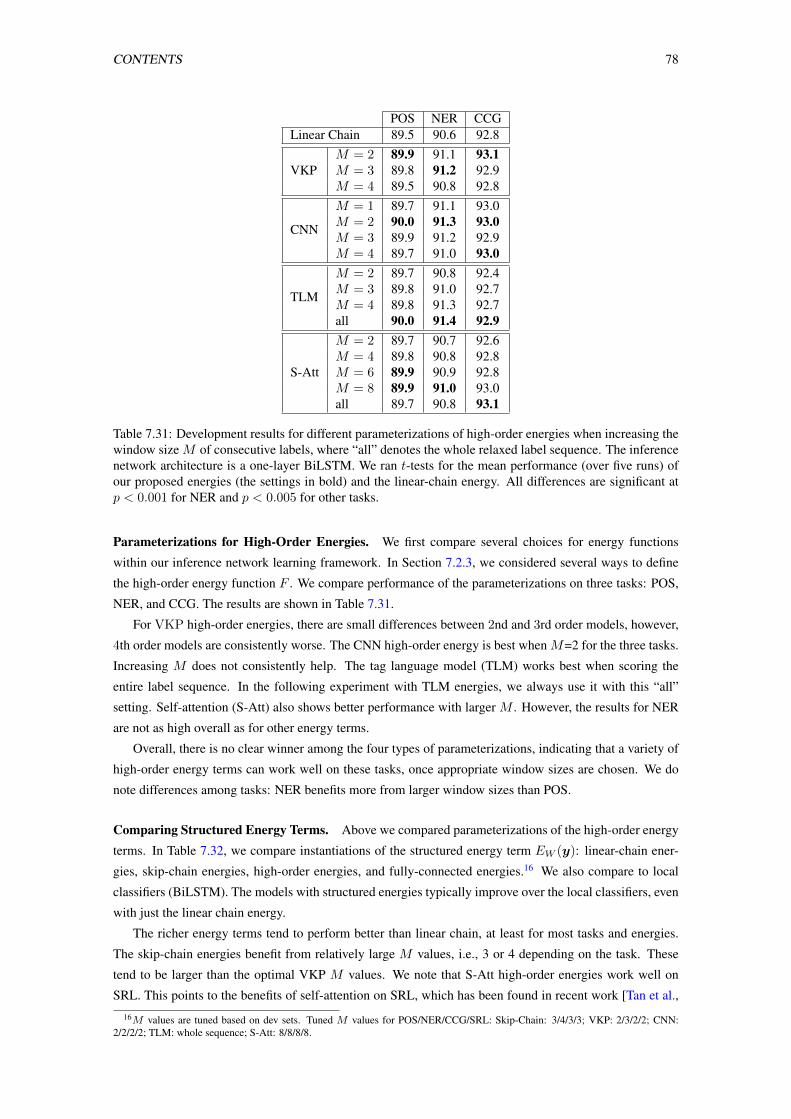
CONTENTS 78
POS NER CCGLinear Chain 89.5 90.6 92.8
VKPM = 2 89.9 91.1 93.1M = 3 89.8 91.2 92.9M = 4 89.5 90.8 92.8M = 1 89.7 91.1 93.0
CNN M = 2 90.0 91.3 93.0M = 3 89.9 91.2 92.9M = 4 89.7 91.0 93.0M = 2 89.7 90.8 92.4
TLM M = 3 89.8 91.0 92.7M = 4 89.8 91.3 92.7all 90.0 91.4 92.9M = 2 89.7 90.7 92.6M = 4 89.8 90.8 92.8
S-Att M = 6 89.9 90.9 92.8M = 8 89.9 91.0 93.0all 89.7 90.8 93.1
Table 7.31: Development results for different parameterizations of high-order energies when increasing thewindow size M of consecutive labels, where “all” denotes the whole relaxed label sequence. The inferencenetwork architecture is a one-layer BiLSTM. We ran t-tests for the mean performance (over five runs) ofour proposed energies (the settings in bold) and the linear-chain energy. All differences are significant atp < 0.001 for NER and p < 0.005 for other tasks.
Parameterizations for High-Order Energies. We first compare several choices for energy functions
within our inference network learning framework. In Section 7.2.3, we considered several ways to define
the high-order energy function F . We compare performance of the parameterizations on three tasks: POS,
NER, and CCG. The results are shown in Table 7.31.
For VKP high-order energies, there are small differences between 2nd and 3rd order models, however,
4th order models are consistently worse. The CNN high-order energy is best when M=2 for the three tasks.
Increasing M does not consistently help. The tag language model (TLM) works best when scoring the
entire label sequence. In the following experiment with TLM energies, we always use it with this “all”
setting. Self-attention (S-Att) also shows better performance with larger M . However, the results for NER
are not as high overall as for other energy terms.
Overall, there is no clear winner among the four types of parameterizations, indicating that a variety of
high-order energy terms can work well on these tasks, once appropriate window sizes are chosen. We do
note differences among tasks: NER benefits more from larger window sizes than POS.
Comparing Structured Energy Terms. Above we compared parameterizations of the high-order energy
terms. In Table 7.32, we compare instantiations of the structured energy term EW (y): linear-chain ener-
gies, skip-chain energies, high-order energies, and fully-connected energies.16 We also compare to local
classifiers (BiLSTM). The models with structured energies typically improve over the local classifiers, even
with just the linear chain energy.
The richer energy terms tend to perform better than linear chain, at least for most tasks and energies.
The skip-chain energies benefit from relatively large M values, i.e., 3 or 4 depending on the task. These
tend to be larger than the optimal VKP M values. We note that S-Att high-order energies work well on
SRL. This points to the benefits of self-attention on SRL, which has been found in recent work [Tan et al.,
16M values are tuned based on dev sets. Tuned M values for POS/NER/CCG/SRL: Skip-Chain: 3/4/3/3; VKP: 2/3/2/2; CNN:2/2/2/2; TLM: whole sequence; S-Att: 8/8/8/8.
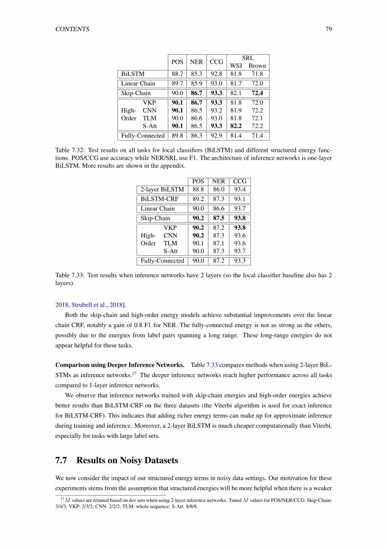
CONTENTS 79
POS NER CCG SRLWSJ Brown
BiLSTM 88.7 85.3 92.8 81.8 71.8Linear Chain 89.7 85.9 93.0 81.7 72.0Skip-Chain 90.0 86.7 93.3 82.1 72.4
VKP 90.1 86.7 93.3 81.8 72.0High- CNN 90.1 86.5 93.2 81.9 72.2Order TLM 90.0 86.6 93.0 81.8 72.1
S-Att 90.1 86.5 93.3 82.2 72.2Fully-Connected 89.8 86.3 92.9 81.4 71.4
Table 7.32: Test results on all tasks for local classifiers (BiLSTM) and different structured energy func-tions. POS/CCG use accuracy while NER/SRL use F1. The architecture of inference networks is one-layerBiLSTM. More results are shown in the appendix.
POS NER CCG2-layer BiLSTM 88.8 86.0 93.4BiLSTM-CRF 89.2 87.3 93.1Linear Chain 90.0 86.6 93.7Skip-Chain 90.2 87.5 93.8
VKP 90.2 87.2 93.8High- CNN 90.2 87.3 93.6Order TLM 90.1 87.1 93.6
S-Att 90.0 87.3 93.7Fully-Connected 90.0 87.2 93.3
Table 7.33: Test results when inference networks have 2 layers (so the local classifier baseline also has 2layers).
2018, Strubell et al., 2018].
Both the skip-chain and high-order energy models achieve substantial improvements over the linear
chain CRF, notably a gain of 0.8 F1 for NER. The fully-connected energy is not as strong as the others,
possibly due to the energies from label pairs spanning a long range. These long-range energies do not
appear helpful for these tasks.
Comparison using Deeper Inference Networks. Table 7.33 compares methods when using 2-layer BiL-
STMs as inference networks.17 The deeper inference networks reach higher performance across all tasks
compared to 1-layer inference networks.
We observe that inference networks trained with skip-chain energies and high-order energies achieve
better results than BiLSTM-CRF on the three datasets (the Viterbi algorithm is used for exact inference
for BiLSTM-CRF). This indicates that adding richer energy terms can make up for approximate inference
during training and inference. Moreover, a 2-layer BiLSTM is much cheaper computationally than Viterbi,
especially for tasks with large label sets.
7.7 Results on Noisy Datasets
We now consider the impact of our structured energy terms in noisy data settings. Our motivation for these
experiments stems from the assumption that structured energies will be more helpful when there is a weaker
17M values are retuned based on dev sets when using 2-layer inference networks. Tuned M values for POS/NER/CCG: Skip-Chain:3/4/3; VKP: 2/3/2; CNN: 2/2/2; TLM: whole sequence; S-Att: 8/8/8.
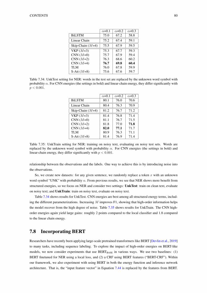
CONTENTS 80
α=0.1 α=0.2 α=0.3BiLSTM 75.0 67.2 58.8Linear Chain 75.2 67.4 59.1Skip-Chain (M=4) 75.5 67.9 59.5VKP (M=3) 75.3 67.7 59.3CNN (M=0) 75.7 67.9 59.4CNN (M=2) 76.3 68.6 60.2CNN (M=4) 76.7 69.8 60.4TLM 76.0 67.8 59.9S-Att (M=8) 75.6 67.6 59.7
Table 7.34: UnkTest setting for NER: words in the test set are replaced by the unknown word symbol withprobability α. For CNN energies (the settings in bold) and linear-chain energy, they differ significantly withp < 0.001.
α=0.1 α=0.2 α=0.3BiLSTM 80.1 76.0 70.6Linear Chain 80.4 76.3 70.9Skip-Chain (M=4) 81.2 76.7 71.2VKP (M=3) 81.4 76.8 71.4CNN (M=0) 81.1 76.7 71.5CNN (M=2) 81.8 77.0 71.8CNN (M=4) 82.0 77.1 71.7TLM 80.9 76.3 71.1S-Att (M=8) 81.4 76.9 71.4
Table 7.35: UnkTrain setting for NER: training on noisy text, evaluating on noisy test sets. Words arereplaced by the unknown word symbol with probability α. For CNN energies (the settings in bold) andlinear-chain energy, they differ significantly with p < 0.001.
relationship between the observations and the labels. One way to achieve this is by introducing noise into
the observations.
So, we create new datasets: for any given sentence, we randomly replace a token x with an unknown
word symbol “UNK” with probability α. From previous results, we see that NER shows more benefit from
structured energies, so we focus on NER and consider two settings: UnkTest: train on clean text, evaluate
on noisy text; and UnkTrain: train on noisy text, evaluate on noisy text.
Table 7.34 shows results for UnkTest. CNN energies are best among all structured energy terms, includ-
ing the different parameterizations. Increasing M improves F1, showing that high-order information helps
the model recover from the high degree of noise. Table 7.35 shows results for UnkTrain. The CNN high-
order energies again yield large gains: roughly 2 points compared to the local classifier and 1.8 compared
to the linear chain energy.
7.8 Incorporating BERT
Researchers have recently been applying large-scale pretrained transformers like BERT [Devlin et al., 2019]
to many tasks, including sequence labeling. To explore the impact of high-order energies on BERT-like
models, we now consider experiments that use BERTBASE in various ways. We use two baselines: (1)
BERT finetuned for NER using a local loss, and (2) a CRF using BERT features (“BERT-CRF”). Within
our framework, we also experiment with using BERT in both the energy function and inference network
architecture. That is, the “input feature vector” in Equation 7.44 is replaced by the features from BERT.
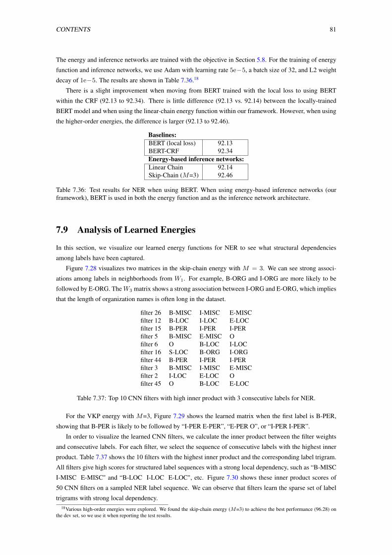
CONTENTS 81
The energy and inference networks are trained with the objective in Section 5.8. For the training of energy
function and inference networks, we use Adam with learning rate 5e−5, a batch size of 32, and L2 weight
decay of 1e−5. The results are shown in Table 7.36.18
There is a slight improvement when moving from BERT trained with the local loss to using BERT
within the CRF (92.13 to 92.34). There is little difference (92.13 vs. 92.14) between the locally-trained
BERT model and when using the linear-chain energy function within our framework. However, when using
the higher-order energies, the difference is larger (92.13 to 92.46).
Baselines:BERT (local loss) 92.13BERT-CRF 92.34Energy-based inference networks:Linear Chain 92.14Skip-Chain (M=3) 92.46
Table 7.36: Test results for NER when using BERT. When using energy-based inference networks (ourframework), BERT is used in both the energy function and as the inference network architecture.
7.9 Analysis of Learned Energies
In this section, we visualize our learned energy functions for NER to see what structural dependencies
among labels have been captured.
Figure 7.28 visualizes two matrices in the skip-chain energy with M = 3. We can see strong associ-
ations among labels in neighborhoods from W1. For example, B-ORG and I-ORG are more likely to be
followed by E-ORG. TheW3 matrix shows a strong association between I-ORG and E-ORG, which implies
that the length of organization names is often long in the dataset.
filter 26 B-MISC I-MISC E-MISCfilter 12 B-LOC I-LOC E-LOCfilter 15 B-PER I-PER I-PERfilter 5 B-MISC E-MISC Ofilter 6 O B-LOC I-LOCfilter 16 S-LOC B-ORG I-ORGfilter 44 B-PER I-PER I-PERfilter 3 B-MISC I-MISC E-MISCfilter 2 I-LOC E-LOC Ofilter 45 O B-LOC E-LOC
Table 7.37: Top 10 CNN filters with high inner product with 3 consecutive labels for NER.
For the VKP energy with M=3, Figure 7.29 shows the learned matrix when the first label is B-PER,
showing that B-PER is likely to be followed by “I-PER E-PER”, “E-PER O”, or “I-PER I-PER”.
In order to visualize the learned CNN filters, we calculate the inner product between the filter weights
and consecutive labels. For each filter, we select the sequence of consecutive labels with the highest inner
product. Table 7.37 shows the 10 filters with the highest inner product and the corresponding label trigram.
All filters give high scores for structured label sequences with a strong local dependency, such as “B-MISC
I-MISC E-MISC" and “B-LOC I-LOC E-LOC", etc. Figure 7.30 shows these inner product scores of
50 CNN filters on a sampled NER label sequence. We can observe that filters learn the sparse set of label
trigrams with strong local dependency.18Various high-order energies were explored. We found the skip-chain energy (M=3) to achieve the best performance (96.28) on
the dev set, so we use it when reporting the test results.
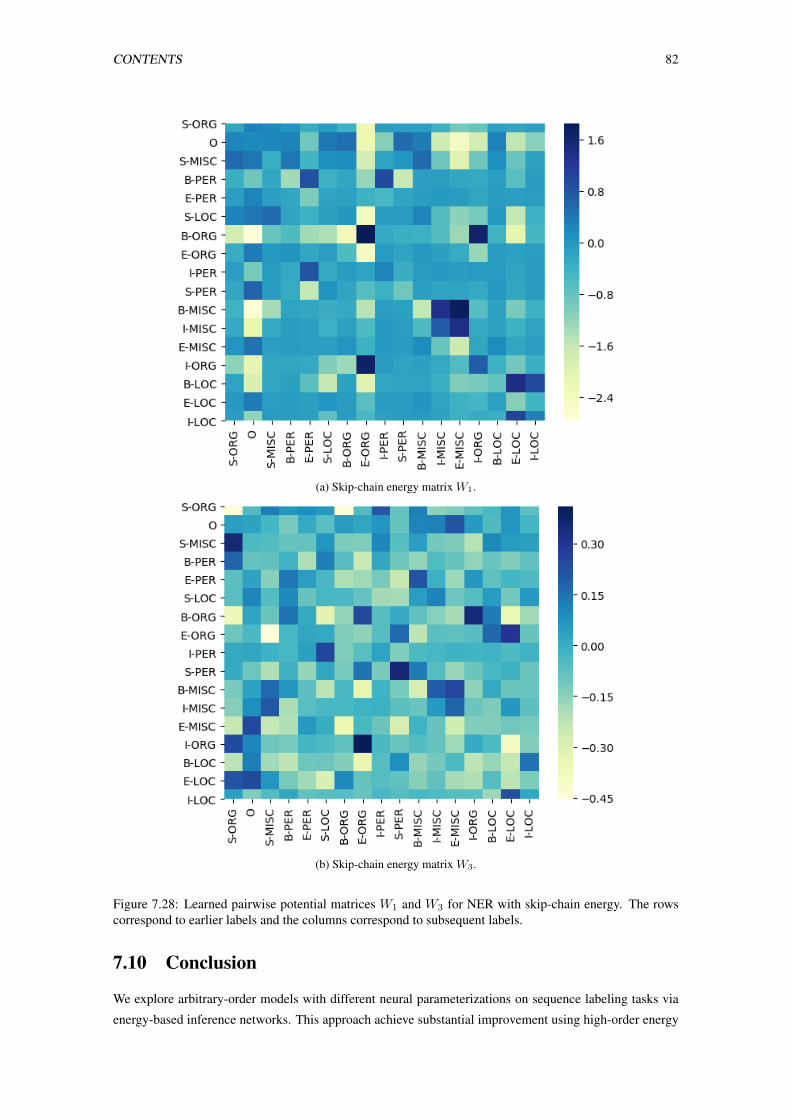
CONTENTS 82
(a) Skip-chain energy matrix W1.
(b) Skip-chain energy matrix W3.
Figure 7.28: Learned pairwise potential matrices W1 and W3 for NER with skip-chain energy. The rowscorrespond to earlier labels and the columns correspond to subsequent labels.
7.10 Conclusion
We explore arbitrary-order models with different neural parameterizations on sequence labeling tasks via
energy-based inference networks. This approach achieve substantial improvement using high-order energy
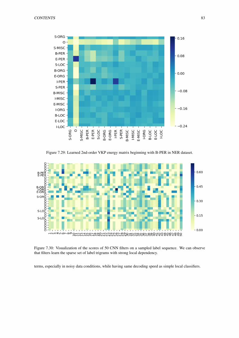
CONTENTS 83
Figure 7.29: Learned 2nd-order VKP energy matrix beginning with B-PER in NER dataset.
Figure 7.30: Visualization of the scores of 50 CNN filters on a sampled label sequence. We can observethat filters learn the sparse set of label trigrams with strong local dependency.
terms, especially in noisy data conditions, while having same decoding speed as simple local classifiers.

Conclusion and Future Work
We conclude this thesis by summarizing our key contribution and discussing some directions of future
research.
9.1 Summary of Contributions
In this thesis, we made the following contributions:
• We summarize the history of energy-based models and several commonly used learning and inference
methods. Especially, what are the main benefit and difficulties of energy-based models (Chapter 1
and Chapter 2)? What is the connection of previous models (Chapter 2)? We also show several wildly
used energy-based models in structured application in NLP (Chapter 2). This can be useful material
for people who are interested in energy-based models.
• For the structure tasks, the inference problem is very challenging due to the exponential large label
space. Previously, the Viterbi algorithm and gradient descent were used for inference if considering
structured components of complex NLP tasks. We develop a new decoding method called “energy-based inference network” which outputs structured continuous values. In our method, the time
complexity for the inference is linear with the label set size. In Chapter 3, we shows “energy-based
inference network” achieves a better speed/accuracy/search error trade off than gradient descent,
while also being faster than exact inference at similar accuracy levels.
• We have worked on several NLP tasks, including multi-label classification, part-of-speech tagging,
named entity recognition, semantic role labeling, and non-autoregressive machine translation. We
train a non-autoregressive machine translation model to minimize the energy defined by a pretrained
autoregressive model, which achieves state-of-the-art non-autoregressive results on the IWSLT 2014
DE-EN and WMT 2016 RO-EN datasets, approaching the performance of autoregressive models.
This indicates that the methods can be very possibly applied to a larger set of applications, especially
more text-based generation tasks.
• We also design a margin-based method for training energy-based models such as linear-chain CRF
or high-order CRF. According to the visualization of the energy and performance improvements, we
demonstrate We empirically demonstrate that this approach achieves substantial improvement using
a variety of high-order energy terms on four sequence labeling tasks while having the same decoding
speed as simple, local classifiers. We also find high-order energies to help in noisy data conditions.
9.2 Future Work
In this section, we propose several future directions.
84
CONTENTS 85
9.2.1 Exploring Energy Terms
We use the linear-chain CRF energy, Tag Language model and high-order energy terms for sequence label-
ing task. It is worth to explore some other energy terms to capture complex label dependency. These terms
can be used for sequence labeling or text generation tasks.
Language Coherence Terms The way to improve the language coherence, we could use an additional
energy term, the log-likelihood of y under the pretrained language models. The standard LSTM language
model or the masked language model(e.g., BERT [Devlin et al., 2019], RoBERTa [Liu et al., 2019]). The
pretrained language models are the vital resources to exploit large monolingual corpora for NMT in our
framework.
Another approach for the repetition is modeling coverage of the source sentence [Tu et al., 2016, Mi
et al., 2016]. And Holtzman et al. [2018] designed an energy term specifically targeting the prevention of
repetition in the output.
Relating Attention to Alignment Since the learned attention function may diverge from alignment pat-
terns between languages, several researchers have experimented with adding inductive biases to the atten-
tion function [Cohn et al., 2016, Feng et al., 2016]. This is often motivated by known characteristics about
the alignment between the source and target language, particularly those related to monotonicity, distortion,
and fertility. It is worth to try similar terms with [Cohn et al., 2016, Feng et al., 2016].
Local Cross Entropy Term The standard log-likelihood scoring function that is used by nearly all NMT
systems. However, it is still not explored how to incorporate the standard cross entropy term with the
other proposed energy terms. According to sequence labeling experiments results in Chapter 5, chapter
6, and chapter 7, the local cross entropy loss could contribute the performance of the inference networks.
The weight for the term can be carefully tuned for higher performance. In Chapter 3, we use the weight
annealing scheme.
However, the local cross entropy term has some limitations: it does not assign partial credit to the
hypotheses if the word order of hypotheses is different from the reference and it could penalize semantically
correct hypotheses if they differ lexically from the reference.
BLEU Recently, there are several work that directly optimize the evaluation metrics such as BLEU to
improve the translation systems. The only issue is that we need to consider how to do backpropagation
through the non-differentiable term. With the similar approximate BLEU from Tromble et al. [2008], we
could directly optimized the BLEU score for translation task or other generation tasks.
Beyond BLEU Wieting et al. [2019] proposes a new metric based on semantic similarity in order to
get partial credit and reduces the penalties on semantically correct hypotheses. This term could potentially
lead the inference networks search better hypotheses with semantically similar hypotheses. The embedding
model to evaluate similarity allows the range of possible scores to be continuous. The inference networks
could get the gradient directly from the term.
SIM(r, h) = cos(g(r), g(h)) (9.46)
where r is the reference and h are the generate hypothesis. g is the encoder for a token sequence. Further-
more, one variation of the metric could be based on the semantic similarity between the source sentence

CONTENTS 86
and the hypotheses. This term potentially fine-tuning the hypotheses that have different semantic meaning
from source sentence.
9.2.2 Learning Methods for Energy-based Models
In our work , we use margin-based training metric for the energy function training. The objective for the
energy function is:
Θ← argminΘ
[4 (FΦ(x),yi)−EΘ(xi,FΦ(x)) + EΘ(xi,yi)
]+
or training two inference networks FΦ and AΨ jointly,
Θ← argminΘ
[4 (FΦ(x),yi)−EΘ(xi,FΦ(x)) + EΘ(xi,yi)
]+
+ λ[− EΘ(xi,AΨ(xi)) + EΘ(xi,yi)
]+
The other interesting approach for energy training is noise-contrastive estimation [Gutmann and Hyvari-
nen, 2010, Wang and Ou, 2018b,a, Bakhtin et al., 2020] (NCE). NCE is proposed for learning unnormalized
statistical models. It use logistic regression to discriminate between the data samples drawn from the data
distribution and noise samples drawn from a noise distribution. They assume that the learned models are
“self-normalized”.
It would be interesting to see some analysis on two different approaches. Or as we know, NCE need a
predefined well-formed noise distribution. So it is hard to inject “domain knowledge“ of text understand-
ing. We can add “negative examples” even the noise distribution form is unknown. In addition, inference
networks can model more complex noise distribution so that a better energy model can be learned.
Bibliography
A. Akbik, D. Blythe, and R. Vollgraf. Contextual string embeddings for sequence labeling. In Proceedings
of the 27th International Conference on Computational Linguistics, pages 1638–1649, Santa Fe, New
Mexico, USA, Aug. 2018. Association for Computational Linguistics. URL https://www.aclweb.
org/anthology/C18-1139.
B. Amos, L. Xu, and J. Z. Kolter. Input convex neural networks. In Proc. of ICML, 2017.
M. Arjovsky, S. Chintala, and L. Bottou. Wasserstein generative adversarial networks. In Proceedings of
the 34th International Conference on Machine Learning, 2017.
J. Ba and R. Caruana. Do deep nets really need to be deep? In Advances in NIPS, 2014.
D. Bahdanau, K. Cho, and Y. Bengio. Neural machine translation by jointly learning to align and translate.
In Proceedings of International Conference on Learning Representations (ICLR), 2015.
D. Bahdanau, P. Brakel, K. Xu, A. Goyal, R. Lowe, J. Pineau, A. C. Courville, and Y. Bengio. An actor-
critic algorithm for sequence prediction. ArXiv, abs/1607.07086, 2017.
A. Bakhtin, Y. Deng, S. Gross, M. Ott, M. Ranzato, and A. Szlam. Energy-based models for text, 2020.
A. G. Barto, R. S. Sutton, and C. W. Anderson. Neuronlike adaptive elements that can solve difficult
learning control problems. IEEE Transactions on Systems, Man, and Cybernetics, SMC-13(5):834–846,
1983. doi: 10.1109/TSMC.1983.6313077.
D. Belanger and A. McCallum. Structured prediction energy networks. In Proceedings of the 33rd Inter-
national Conference on Machine Learning - Volume 48, ICML’16, pages 983–992, 2016.
D. Belanger, B. Yang, and A. McCallum. End-to-end learning for structured prediction energy networks.
In Proc. of ICML, 2017.
Y. Bengio and J.-S. Senecal. Quick training of probabilistic neural nets by importance sampling. In AIS-
TATS, 2003.
Y. Bengio, R. Ducharme, and P. Vincent. A neural probabilistic language model. In T. Leen, T. Dietterich,
and V. Tresp, editors, Advances in Neural Information Processing Systems. MIT Press, 2001.
Y. Bengio, N. Léonard, and A. Courville. Estimating or propagating gradients through stochastic neurons
for conditional computation. arXiv preprint arXiv:1308.3432, 2013.
L. Bottou. Une Approche théorique de l’Apprentissage Connexionniste: Applications à la Reconnaissance
de la Parole. PhD thesis, Université de Paris XI, Orsay, France, 1991. URL http://leon.bottou.
org/papers/bottou-91a.
87
BIBLIOGRAPHY 88
S. Calhoun, J. Carletta, J. M. Brenier, N. Mayo, D. Jurafsky, M. Steedman, and D. Beaver. The NXT-format
Switchboard Corpus: a rich resource for investigating the syntax, semantics, pragmatics and prosody of
dialogue. Language resources and evaluation, 44(4):387–419, 2010.
X. Carreras and L. Màrquez. Introduction to the CoNLL-2005 shared task: Semantic role labeling. In
Proceedings of the Ninth Conference on Computational Natural Language Learning (CoNLL-2005),
pages 152–164, Ann Arbor, Michigan, June 2005. Association for Computational Linguistics. URL
https://www.aclweb.org/anthology/W05-0620.
K.-W. Chang, S. Upadhyay, G. Kundu, and D. Roth. Structural learning with amortized inference. In Proc.
of AAAI, 2015.
Y. Chen, V. O. Li, K. Cho, and S. Bowman. A stable and effective learning strategy for trainable greedy
decoding. In Proceedings of the 2018 Conference on Empirical Methods in Natural Language Process-
ing, pages 380–390, Brussels, Belgium, Oct.-Nov. 2018. Association for Computational Linguistics. doi:
10.18653/v1/D18-1035. URL https://www.aclweb.org/anthology/D18-1035.
D. Chiang. Hierarchical phrase-based translation. Computational Linguistics, 33(2):201–228, 2007. doi:
10.1162/coli.2007.33.2.201. URL https://www.aclweb.org/anthology/J07-2003.
W. W. Cohen and V. R. de Carvalho. Stacked sequential learning. In IJCAI-05, Proceedings of the Nine-
teenth International Joint Conference on Artificial Intelligence, Edinburgh, Scotland, UK, July 30 - Au-
gust 5, 2005, pages 671–676, 2005. URL http://ijcai.org/Proceedings/05/Papers/
0378.pdf.
W. W. Cohen, R. E. Schapire, and Y. Singer. Learning to order things. In Advances in Neural Information
Processing Systems, 1998.
T. Cohn, C. D. V. Hoang, E. Vymolova, K. Yao, C. Dyer, and G. Haffari. Incorporating structural alignment
biases into an attentional neural translation model. In Proceedings of the 2016 Conference of the North
American Chapter of the Association for Computational Linguistics: Human Language Technologies,
pages 876–885, San Diego, California, June 2016. Association for Computational Linguistics. doi: 10.
18653/v1/N16-1102. URL https://www.aclweb.org/anthology/N16-1102.
M. Collins. Discriminative training methods for hidden Markov models: Theory and experiments with
perceptron algorithms. In Proc. of EMNLP, 2002.
R. Collobert, J. Weston, L. Bottou, M. Karlen, K. Kavukcuoglu, and P. P. Kuksa. Natural language process-
ing (almost) from scratch. Journal of Machine Learning Research, 12:2493–2537, 2011.
G. F. Cooper. The computational complexity of probabilistic inference using Bayesian belief networks
(research note). Artif. Intell., 42(2-3), Mar. 1990.
C. Cortes and V. Vapnik. Support vector networks. Machine Learning, 1995.
N. V. Cuong, N. Ye, W. S. Lee, and H. L. Chieu. Conditional random field with high-order dependencies for
sequence labeling and segmentation. Journal of Machine Learning Research, 15(28):981–1009, 2014.
URL http://jmlr.org/papers/v15/cuong14a.html.
Z. Dai, A. Almahairi, B. Philip, E. Hovy, and A. Courville. Calibrating energy-based generative adversarial
networks. In Proc. of ICLR, 2017.
BIBLIOGRAPHY 89
J. Devlin, M.-W. Chang, K. Lee, and K. Toutanova. BERT: Pre-training of deep bidirectional transformers
for language understanding. In Proceedings of the 2019 Conference of the North American Chapter of the
Association for Computational Linguistics: Human Language Technologies, Volume 1 (Long and Short
Papers), pages 4171–4186, Minneapolis, Minnesota, June 2019. Association for Computational Linguis-
tics. doi: 10.18653/v1/N19-1423. URL https://www.aclweb.org/anthology/N19-1423.
J. Domke. Generic methods for optimization-based modeling. In Proc. of AISTATS, 2012.
J. Duchi, E. Hazan, and Y. Singer. Adaptive subgradient methods for online learning and stochastic opti-
mization. 2011.
C. Dyer. Notes on noise contrastive estimation and negative sampling. CoRR, abs/1410.8251, 2014. URL
http://arxiv.org/abs/1410.8251.
S. Edunov, M. Ott, M. Auli, D. Grangier, and M. Ranzato. Classical structured prediction losses for se-
quence to sequence learning. In Proceedings of the 2018 Conference of the North American Chapter
of the Association for Computational Linguistics: Human Language Technologies, Volume 1 (Long Pa-
pers), pages 355–364, New Orleans, Louisiana, June 2018. Association for Computational Linguistics.
doi: 10.18653/v1/N18-1033. URL https://www.aclweb.org/anthology/N18-1033.
S. Feng, S. Liu, N. Yang, M. Li, M. Zhou, and K. Q. Zhu. Improving attention modeling with im-
plicit distortion and fertility for machine translation. In Proceedings of COLING 2016, the 26th In-
ternational Conference on Computational Linguistics: Technical Papers, pages 3082–3092, Osaka,
Japan, Dec. 2016. The COLING 2016 Organizing Committee. URL https://www.aclweb.org/
anthology/C16-1290.
J. R. Finkel, T. Grenager, and C. Manning. Incorporating non-local information into information extrac-
tion systems by Gibbs sampling. In Proceedings of the 43rd Annual Meeting of the Association for
Computational Linguistics (ACL’05), pages 363–370, Ann Arbor, Michigan, June 2005. Association for
Computational Linguistics. doi: 10.3115/1219840.1219885. URL https://www.aclweb.org/
anthology/P05-1045.
L. A. Gatys, A. S. Ecker, and M. Bethge. A neural algorithm of artistic style. CoRR, abs/1508.06576, 2015.
K. J. Geras, A. rahman Mohamed, R. Caruana, G. Urban, S. Wang, O. Aslan, M. Philipose, M. Richardson,
and C. Sutton. Blending LSTMs into CNNs. In Proc. of ICLR (workshop track), 2016.
S. Gershman and N. Goodman. Amortized inference in probabilistic reasoning. In Proc. of the Cognitive
Science Society, 2014.
M. Ghazvininejad, O. Levy, Y. Liu, and L. Zettlemoyer. Mask-predict: Parallel decoding of conditional
masked language models. In Proceedings of the 2019 Conference on Empirical Methods in Natural Lan-
guage Processing and the 9th International Joint Conference on Natural Language Processing (EMNLP-
IJCNLP), pages 6111–6120, Hong Kong, China, Nov. 2019. Association for Computational Linguistics.
doi: 10.18653/v1/D19-1633. URL https://www.aclweb.org/anthology/D19-1633.
M. Ghazvininejad, V. Karpukhin, L. Zettlemoyer, and O. Levy. Aligned cross entropy for non-
autoregressive machine translation. arXiv preprint arXiv:2004.01655, 2020.
K. Gimpel, N. Schneider, B. O’Connor, D. Das, D. Mills, J. Eisenstein, M. Heilman, D. Yogatama, J. Flani-
gan, and N. A. Smith. Part-of-speech tagging for twitter: Annotation, features, and experiments. In
BIBLIOGRAPHY 90
Proceedings of the 49th Annual Meeting of the Association for Computational Linguistics: Human Lan-
guage Technologies, pages 42–47, Portland, Oregon, USA, June 2011. Association for Computational
Linguistics. URL https://www.aclweb.org/anthology/P11-2008.
I. Goodfellow, J. Pouget-Abadie, M. Mirza, B. Xu, D. Warde-Farley, S. Ozair, A. Courville, and Y. Bengio.
Generative adversarial nets. In Advances in NIPS, 2014.
K. Goyal, G. Neubig, C. Dyer, and T. Berg-Kirkpatrick. A continuous relaxation of beam search for end-
to-end training of neural sequence models. In Proc. of AAAI, 2018.
C. Graber and A. G. Schwing. Graph Structured Prediction Energy Networks. In Proc. NeurIPS, 2019.
C. Graber, O. Meshi, and A. Schwing. Deep structured prediction with nonlinear output
transformations. In S. Bengio, H. Wallach, H. Larochelle, K. Grauman, N. Cesa-Bianchi,
and R. Garnett, editors, Advances in Neural Information Processing Systems 31, pages
6320–6331. Curran Associates, Inc., 2018. URL http://papers.nips.cc/paper/
7869-deep-structured-prediction-with-nonlinear-output-transformations.
pdf.
W. Grathwohl, K.-C. Wang, J.-H. Jacobsen, D. Duvenaud, M. Norouzi, and K. Swersky. Your classifier is
secretly an energy based model and you should treat it like one. In International Conference on Learning
Representations, 2020. URL https://openreview.net/forum?id=Hkxzx0NtDB.
J. Gu, K. Cho, and V. O. Li. Trainable greedy decoding for neural machine translation. In Proceedings of
the 2017 Conference on Empirical Methods in Natural Language Processing, pages 1968–1978, Copen-
hagen, Denmark, Sept. 2017. Association for Computational Linguistics. doi: 10.18653/v1/D17-1210.
URL https://www.aclweb.org/anthology/D17-1210.
J. Gu, J. Bradbury, C. Xiong, V. O. Li, and R. Socher. Non-autoregressive neural machine translation. In
Proceedings of International Conference on Learning Representations (ICLR), 2018.
C. Gulcehre, O. Firat, K. Xu, K. Cho, L. Barrault, H.-C. Lin, F. Bougares, H. Schwenk, and Y. Bengio. On
Using Monolingual Corpora in Neural Machine Translation. arXiv e-prints, 2015.
I. Gulrajani, F. Ahmed, M. Arjovsky, V. Dumoulin, and A. C. Courville. Improved train-
ing of Wasserstein GANs. In I. Guyon, U. V. Luxburg, S. Bengio, H. Wallach,
R. Fergus, S. Vishwanathan, and R. Garnett, editors, Advances in Neural Information Pro-
cessing Systems 30, pages 5767–5777. 2017. URL http://papers.nips.cc/paper/
7159-improved-training-of-wasserstein-gans.pdf.
M. Gutmann and A. Hyvarinen. Noise-contrastive estimation: A new estimation principle for unnormalized
statistical models. In Proceedings of the Thirteenth International Conference on Artificial Intelligence
and Statistics, 2010.
M. Gygli, M. Norouzi, and A. Angelova. Deep value networks learn to evaluate and iteratively refine
structured outputs. In ICML, 2017.
F. Hill, A. Bordes, S. Chopra, and J. Weston. The goldilocks principle: Reading children’s books with
explicit memory representations. In Y. Bengio and Y. LeCun, editors, 4th International Conference
on Learning Representations, ICLR 2016, San Juan, Puerto Rico, May 2-4, 2016, Conference Track
Proceedings, 2016.
BIBLIOGRAPHY 91
G. Hinton, O. Vinyals, and J. Dean. Distilling the knowledge in a neural network. In NIPS Deep Learning
Workshop, 2015.
G. E. Hinton. Training Products of Experts by Minimizing Contrastive Divergence. Neural Computation,
2002.
G. E. Hinton, N. Srivastava, A. Krizhevsky, I. Sutskever, and R. Salakhutdinov. Improving neural networks
by preventing co-adaptation of feature detectors. CoRR, abs/1207.0580, 2012.
C. D. V. Hoang, G. Haffari, and T. Cohn. Towards decoding as continuous optimisation in neural machine
translation. In Proc. of EMNLP, 2017.
S. Hochreiter and J. Schmidhuber. Long short-term memory. Neural Computation, 1997.
J. Hockenmaier and M. Steedman. Acquiring compact lexicalized grammars from a cleaner treebank. In
Proceedings of the Third International Conference on Language Resources and Evaluation (LREC’02),
Las Palmas, Canary Islands - Spain, May 2002. European Language Resources Association (ELRA).
URL http://www.lrec-conf.org/proceedings/lrec2002/pdf/263.pdf.
A. Holtzman, J. Buys, M. Forbes, A. Bosselut, D. Golub, and Y. Choi. Learning to write with coopera-
tive discriminators. In Proceedings of the 56th Annual Meeting of the Association for Computational
Linguistics (Volume 1: Long Papers), pages 1638–1649, Melbourne, Australia, July 2018. Association
for Computational Linguistics. doi: 10.18653/v1/P18-1152. URL https://www.aclweb.org/
anthology/P18-1152.
K. Hu, Z. Ou, M. Hu, and J. Feng. Neural crf transducers for sequence labeling. In ICASSP 2019 - 2019
IEEE International Conference on Acoustics, Speech and Signal Processing (ICASSP), pages 2997–3001,
2019.
L. Huang and D. Chiang. Forest rescoring: Faster decoding with integrated language models. In Pro-
ceedings of the 45th Annual Meeting of the Association of Computational Linguistics, pages 144–
151, Prague, Czech Republic, June 2007. Association for Computational Linguistics. URL https:
//www.aclweb.org/anthology/P07-1019.
Z. Huang, W. Xu, and K. Yu. Bidirectional LSTM-CRF models for sequence tagging. CoRR,
abs/1508.01991, 2015. URL http://arxiv.org/abs/1508.01991.
J.-J. Hwang, T.-W. Ke, J. Shi, and S. X. Yu. Adversarial structure matching for structured prediction tasks.
In Proceedings of the IEEE Conference on Computer Vision and Pattern Recognition, pages 4056–4065,
2019.
A. Hyvärinen. Estimation of non-normalized statistical models by score matching. Journal of
Machine Learning Research, 6(24):695–709, 2005. URL http://jmlr.org/papers/v6/
hyvarinen05a.html.
E. Jang, S. Gu, and B. Poole. Categorical reparameterization with gumbel-softmax. In Proceedings of
International Conference on Learning Representations (ICLR), 2016.
F. Jelinek and R. L. Mercer. Interpolated estimation of Markov source parameters from sparse data. In
Proceedings, Workshop on Pattern Recognition in Practice. 1980.
J. Johnson, A. Alahi, and L. Fei-Fei. Perceptual losses for real-time style transfer and super-resolution. In
Proc. of ECCV, 2016.
BIBLIOGRAPHY 92
L. Kaiser, S. Bengio, A. Roy, A. Vaswani, N. Parmar, J. Uszkoreit, and N. Shazeer. Fast decoding in
sequence models using discrete latent variables. In International Conference on Machine Learning,
pages 2395–2404, 2018.
V. Karpukhin, B. Oguz, S. Min, P. Lewis, L. Wu, S. Edunov, D. Chen, and W.-t. Yih. Dense pas-
sage retrieval for open-domain question answering. In Proceedings of the 2020 Conference on Em-
pirical Methods in Natural Language Processing (EMNLP), pages 6769–6781, Online, Nov. 2020.
Association for Computational Linguistics. doi: 10.18653/v1/2020.emnlp-main.550. URL https:
//www.aclweb.org/anthology/2020.emnlp-main.550.
J. Kasai, J. Cross, M. Ghazvininejad, and J. Gu. Parallel machine translation with disentangled context
transformer, 2020.
K.Gimpel. Lecture 10 - inference and learning in structured prediction. 2019.
Y. Kim. Convolutional neural networks for sentence classification. In Proceedings of the 2014 Conference
on Empirical Methods in Natural Language Processing (EMNLP), pages 1746–1751, Doha, Qatar, Oct.
2014. Association for Computational Linguistics. doi: 10.3115/v1/D14-1181. URL https://www.
aclweb.org/anthology/D14-1181.
Y. Kim and A. M. Rush. Sequence-level knowledge distillation. In Proc. of EMNLP, 2016.
D. Kingma and M. Welling. Auto-encoding variational Bayes. CoRR, abs/1312.6114, 2013.
D. P. Kingma and J. Ba. Adam: A method for stochastic optimization. arXiv preprint arXiv:1412.6980,
2014.
D. P. Kingma and J. Ba. Adam: A method for stochastic optimization. In Y. Bengio and Y. LeCun, editors,
3rd International Conference on Learning Representations, ICLR 2015, San Diego, CA, USA, May 7-9,
2015, Conference Track Proceedings, 2015. URL http://arxiv.org/abs/1412.6980.
R. Kiros, R. Salakhutdinov, and R. Zemel. Unifying visual-semantic embeddings with multimodal neural
language models. ArXiv, abs/1411.2539, 2014.
D. Koller and N. Friedman. Probabilistic Graphical Models: Principles and Techniques. 2009.
P. Krähenbühl and V. Koltun. Efficient inference in fully connected CRFs with Gaussian edge potentials.
In Advances in NIPS, 2011.
V. Krishnan and C. D. Manning. An effective two-stage model for exploiting non-local dependencies
in named entity recognition. In Proceedings of the 21st International Conference on Computational
Linguistics and 44th Annual Meeting of the Association for Computational Linguistics, pages 1121–
1128, Sydney, Australia, July 2006. Association for Computational Linguistics. doi: 10.3115/1220175.
1220316. URL https://www.aclweb.org/anthology/P06-1141.
A. Kuncoro, M. Ballesteros, L. Kong, C. Dyer, and N. A. Smith. Distilling an ensemble of greedy depen-
dency parsers into one MST parser. In Proc. of EMNLP, 2016.
J. D. Lafferty, A. McCallum, and F. C. N. Pereira. Conditional random fields: Probabilistic models for
segmenting and labeling sequence data. In Proceedings of the Eighteenth International Conference on
Machine Learning, ICML ’01, pages 282–289, 2001. ISBN 1-55860-778-1.
BIBLIOGRAPHY 93
G. Lample, M. Ballesteros, S. Subramanian, K. Kawakami, and C. Dyer. Neural architectures for named
entity recognition. In Proceedings of the 2016 Conference of the North American Chapter of the As-
sociation for Computational Linguistics: Human Language Technologies, pages 260–270, San Diego,
California, June 2016. Association for Computational Linguistics. doi: 10.18653/v1/N16-1030. URL
https://www.aclweb.org/anthology/N16-1030.
Y. LeCun, S. Chopra, R. Hadsell, M. Ranzato, and F. Huang. A tutorial on energy-based learning. In
Predicting Structured Data. MIT Press, 2006.
J. Lee, E. Mansimov, and K. Cho. Deterministic non-autoregressive neural sequence modeling by iterative
refinement. In Proceedings of the 2018 Conference on Empirical Methods in Natural Language Process-
ing, pages 1173–1182, Brussels, Belgium, Oct.-Nov. 2018. Association for Computational Linguistics.
doi: 10.18653/v1/D18-1149. URL https://www.aclweb.org/anthology/D18-1149.
T. Lei, Y. Xin, Y. Zhang, R. Barzilay, and T. Jaakkola. Low-rank tensors for scoring dependency struc-
tures. In Proceedings of the 52nd Annual Meeting of the Association for Computational Linguistics
(Volume 1: Long Papers), pages 1381–1391, Baltimore, Maryland, June 2014. Association for Compu-
tational Linguistics. doi: 10.3115/v1/P14-1130. URL https://www.aclweb.org/anthology/
P14-1130.
M. Lewis, K. Lee, and L. Zettlemoyer. Lstm ccg parsing. In Proceedings of the 2016 Conference of the
North American Chapter of the Association for Computational Linguistics: Human Language Technolo-
gies, pages 221–231, San Diego, California, June 2016. Association for Computational Linguistics. doi:
10.18653/v1/N16-1026. URL https://www.aclweb.org/anthology/N16-1026.
C. Li and M. Wand. Precomputed real-time texture synthesis with Markovian generative adversarial net-
works. CoRR, abs/1604.04382, 2016.
J. Libovický and J. Helcl. End-to-end non-autoregressive neural machine translation with connection-
ist temporal classification. In Proceedings of the 2018 Conference on Empirical Methods in Natural
Language Processing, pages 3016–3021, Brussels, Belgium, Oct.-Nov. 2018. Association for Computa-
tional Linguistics. doi: 10.18653/v1/D18-1336. URL https://www.aclweb.org/anthology/
D18-1336.
C.-Y. Lin. ROUGE: A package for automatic evaluation of summaries. In Text Summarization Branches
Out, pages 74–81, Barcelona, Spain, July 2004. Association for Computational Linguistics. URL
https://www.aclweb.org/anthology/W04-1013.
Y. Liu, M. Ott, N. Goyal, J. Du, M. Joshi, D. Chen, O. Levy, M. Lewis, L. Zettlemoyer, and V. Stoyanov.
Roberta: A robustly optimized BERT pretraining approach. CoRR, abs/1907.11692, 2019. URL http:
//arxiv.org/abs/1907.11692.
B. T. Lowerre. The HARPY Speech Recognition System. PhD thesis, Pittsburgh, PA, USA, 1976.
T. Luong, H. Pham, and C. D. Manning. Effective approaches to attention-based neural machine translation.
In Proceedings of the 2015 Conference on Empirical Methods in Natural Language Processing, pages
1412–1421, Lisbon, Portugal, Sept. 2015. Association for Computational Linguistics. doi: 10.18653/v1/
D15-1166. URL https://www.aclweb.org/anthology/D15-1166.
X. Ma and E. Hovy. End-to-end sequence labeling via bi-directional LSTM-CNNs-CRF. In Proceedings
of the 54th Annual Meeting of the Association for Computational Linguistics (Volume 1: Long Papers),
BIBLIOGRAPHY 94
pages 1064–1074, Berlin, Germany, Aug. 2016. Association for Computational Linguistics. doi: 10.
18653/v1/P16-1101. URL https://www.aclweb.org/anthology/P16-1101.
X. Ma, C. Zhou, X. Li, G. Neubig, and E. Hovy. FlowSeq: Non-autoregressive conditional sequence gener-
ation with generative flow. In Proceedings of the 2019 Conference on Empirical Methods in Natural Lan-
guage Processing and the 9th International Joint Conference on Natural Language Processing (EMNLP-
IJCNLP), pages 4281–4291, Hong Kong, China, Nov. 2019. Association for Computational Linguistics.
doi: 10.18653/v1/D19-1437. URL https://www.aclweb.org/anthology/D19-1437.
M. P. Marcus, M. A. Marcinkiewicz, and B. Santorini. Building a large annotated corpus of english: The
penn treebank. Comput. Linguist., 1993.
A. Martins, N. Smith, M. Figueiredo, and P. Aguiar. Dual decomposition with many overlapping compo-
nents. In Proceedings of the 2011 Conference on Empirical Methods in Natural Language Processing,
pages 238–249, Edinburgh, Scotland, UK., July 2011. Association for Computational Linguistics. URL
https://www.aclweb.org/anthology/D11-1022.
A. F. T. Martins and J. Kreutzer. Learning what’s easy: Fully differentiable neural easy-first taggers. In
Proc. of EMNLP, 2017.
A. McCallum, D. Freitag, and F. C. N. Pereira. Maximum entropy markov models for information extraction
and segmentation. In Proceedings of the Seventeenth International Conference on Machine Learning,
ICML ’00, 2000.
H. Mi, B. Sankaran, Z. Wang, and A. Ittycheriah. Coverage embedding models for neural machine
translation. In Proceedings of the 2016 Conference on Empirical Methods in Natural Language Pro-
cessing, pages 955–960, Austin, Texas, Nov. 2016. Association for Computational Linguistics. doi:
10.18653/v1/D16-1096. URL https://www.aclweb.org/anthology/D16-1096.
T. Mikolov, I. Sutskever, K. Chen, G. S. Corrado, and J. Dean. Distributed representations of words and
phrases and their compositionality. In Advances in NIPS, 2013.
T. Miyato, T. Kataoka, M. Koyama, and Y. Yoshida. Spectral normalization for generative adversarial
networks. In Proceedings of International Conference on Learning Representations (ICLR), 2018.
H. Mobahi, M. Farajtabar, and P. L. Bartlett. Self-distillation amplifies regularization in hilbert space.
CoRR, abs/2002.05715, 2020. URL https://arxiv.org/abs/2002.05715.
A. Mordvintsev, C. Olah, and M. Tyka. DeepDream-a code example for visualizing neural networks.
Google Research, 2015.
M. Mostajabi, M. Maire, and G. Shakhnarovich. Regularizing deep networks by modeling and predicting
label structure. In Computer Vision and Pattern Recognition (CVPR), 2018.
T. Mueller, H. Schmid, and H. Schütze. Efficient higher-order CRFs for morphological tagging. In
Proceedings of the 2013 Conference on Empirical Methods in Natural Language Processing, pages
322–332, Seattle, Washington, USA, Oct. 2013. Association for Computational Linguistics. URL
https://www.aclweb.org/anthology/D13-1032.
K. P. Murphy, Y. Weiss, and M. I. Jordan. Loopy belief propagation for approximate inference: An empirical
study. In UAI, 1999.
BIBLIOGRAPHY 95
R. M. Neal. Probabilistic inference using markov chain monte carlo methods. Technical report, 1993.
M. Norouzi, S. Bengio, z. Chen, N. Jaitly, M. Schuster, Y. Wu, and D. Schuurmans. Reward aug-
mented maximum likelihood for neural structured prediction. In D. Lee, M. Sugiyama, U. Luxburg,
I. Guyon, and R. Garnett, editors, Advances in Neural Information Processing Systems, volume 29. Cur-
ran Associates, Inc., 2016. URL https://proceedings.neurips.cc/paper/2016/file/
2f885d0fbe2e131bfc9d98363e55d1d4-Paper.pdf.
F. J. Och, D. Gildea, S. Khudanpur, A. Sarkar, K. Yamada, A. Fraser, S. Kumar, L. Shen, D. Smith,
K. Eng, V. Jain, Z. Jin, and D. Radev. A smorgasbord of features for statistical machine transla-
tion. In Proceedings of the Human Language Technology Conference of the North American Chapter
of the Association for Computational Linguistics: HLT-NAACL 2004, pages 161–168, Boston, Mas-
sachusetts, USA, May 2 - May 7 2004. Association for Computational Linguistics. URL https:
//www.aclweb.org/anthology/N04-1021.
O. Owoputi, B. O’Connor, C. Dyer, K. Gimpel, N. Schneider, and N. A. Smith. Improved part-of-speech
tagging for online conversational text with word clusters. In Proceedings of the 2013 Conference of
the North American Chapter of the Association for Computational Linguistics: Human Language Tech-
nologies, pages 380–390, Atlanta, Georgia, June 2013. Association for Computational Linguistics. URL
https://www.aclweb.org/anthology/N13-1039.
B. Paige and F. Wood. Inference networks for sequential Monte Carlo in graphical models. In Proc. of
ICML, 2016.
D. Paperno, G. Kruszewski, A. Lazaridou, N. Q. Pham, R. Bernardi, S. Pezzelle, M. Baroni, G. Boleda, and
R. Fernández. The LAMBADA dataset: Word prediction requiring a broad discourse context. In Pro-
ceedings of the 54th Annual Meeting of the Association for Computational Linguistics (Volume 1: Long
Papers), pages 1525–1534, Berlin, Germany, Aug. 2016. Association for Computational Linguistics. doi:
10.18653/v1/P16-1144. URL https://www.aclweb.org/anthology/P16-1144.
K. Papineni, S. Roukos, T. Ward, and W.-J. Zhu. Bleu: a method for automatic evaluation of machine
translation. In Proceedings of the 40th Annual Meeting of the Association for Computational Linguistics,
pages 311–318, Philadelphia, Pennsylvania, USA, July 2002. Association for Computational Linguistics.
doi: 10.3115/1073083.1073135. URL https://www.aclweb.org/anthology/P02-1040.
A. Passos, V. Kumar, and A. McCallum. Lexicon infused phrase embeddings for named entity resolution.
In Proceedings of the Eighteenth Conference on Computational Natural Language Learning, pages 78–
86, Ann Arbor, Michigan, June 2014. Association for Computational Linguistics. doi: 10.3115/v1/
W14-1609. URL https://www.aclweb.org/anthology/W14-1609.
J. Pennington, R. Socher, and C. Manning. Glove: Global vectors for word representation. In Proceedings
of the 2014 Conference on Empirical Methods in Natural Language Processing (EMNLP), pages 1532–
1543, Doha, Qatar, Oct. 2014. Association for Computational Linguistics. doi: 10.3115/v1/D14-1162.
URL https://www.aclweb.org/anthology/D14-1162.
G. Pereyra, G. Tucker, J. Chorowski, L. Kaiser, and G. E. Hinton. Regularizing neural networks by penal-
izing confident output distributions. CoRR, 2017.
M. Peters, M. Neumann, M. Iyyer, M. Gardner, C. Clark, K. Lee, and L. Zettlemoyer. Deep contextualized
word representations. In Proceedings of the 2018 Conference of the North American Chapter of the
BIBLIOGRAPHY 96
Association for Computational Linguistics: Human Language Technologies, Volume 1 (Long Papers),
pages 2227–2237, New Orleans, Louisiana, June 2018. Association for Computational Linguistics. doi:
10.18653/v1/N18-1202. URL https://www.aclweb.org/anthology/N18-1202.
X. Qian, X. Jiang, Q. Zhang, X. Huang, and L. Wu. Sparse higher order conditional random fields for
improved sequence labeling. In ICML, 2009.
A. Radford, K. Narasimhan, T. Salimans, and I. Sutskever. Improving language understanding by generative
pre-training. In Technical report, OpenAI, 2018.
A. Radford, J. Wu, R. Child, D. Luan, D. Amodei, and I. Sutskever. Language models are unsupervised
multitask learners. 2019.
P. Rajpurkar, J. Zhang, K. Lopyrev, and P. Liang. SQuAD: 100,000+ questions for machine comprehension
of text. In Proceedings of the 2016 Conference on Empirical Methods in Natural Language Processing,
pages 2383–2392, Austin, Texas, Nov. 2016. Association for Computational Linguistics. doi: 10.18653/
v1/D16-1264. URL https://www.aclweb.org/anthology/D16-1264.
M. Ranzato, Y.-L. Boureau, S. Chopra, and Y. LeCun. A unified energy-based framework for unsupervised
learning. In M. Meila and X. Shen, editors, Proceedings of the Eleventh International Conference on
Artificial Intelligence and Statistics, volume 2 of Proceedings of Machine Learning Research, pages
371–379, San Juan, Puerto Rico, 21–24 Mar 2007. PMLR. URL http://proceedings.mlr.
press/v2/ranzato07a.html.
M. Ranzato, S. Chopra, M. Auli, and W. Zaremba. Sequence level training with recurrent neural networks.
In 4th International Conference on Learning Representations, ICLR 2016, San Juan, Puerto Rico, May
2-4, 2016, Conference Track Proceedings, 2016.
L. Ratinov and D. Roth. Design challenges and misconceptions in named entity recognition. In Proceedings
of the Thirteenth Conference on Computational Natural Language Learning (CoNLL-2009), pages 147–
155, June 2009. URL https://www.aclweb.org/anthology/W09-1119.
S. Reddy, D. Chen, and C. D. Manning. CoQA: A conversational question answering challenge. Trans-
actions of the Association for Computational Linguistics, 7:249–266, Mar. 2019. doi: 10.1162/tacl_a_
00266. URL https://www.aclweb.org/anthology/Q19-1016.
D. Roth and W.-t. Yih. A linear programming formulation for global inference in natural language tasks.
In Proceedings of the Eighth Conference on Computational Natural Language Learning (CoNLL-2004)
at HLT-NAACL 2004, pages 1–8, Boston, Massachusetts, USA, May 6 - May 7 2004. Association for
Computational Linguistics. URL https://www.aclweb.org/anthology/W04-2401.
A. M. Rush, D. Sontag, M. Collins, and T. Jaakkola. On dual decomposition and linear programming relax-
ations for natural language processing. In Proceedings of the 2010 Conference on Empirical Methods in
Natural Language Processing, pages 1–11, Cambridge, MA, Oct. 2010. Association for Computational
Linguistics. URL https://www.aclweb.org/anthology/D10-1001.
C. Saharia, W. Chan, S. Saxena, and M. Norouzi. Non-autoregressive machine translation with latent
alignments. arXiv preprint arXiv:2004.07437, 2020.
T. Salimans, I. Goodfellow, W. Zaremba, V. Cheung, A. Radford, and X. Chen. Improved techniques for
training GANs. In D. D. Lee, M. Sugiyama, U. V. Luxburg, I. Guyon, and R. Garnett, editors, Advances in
BIBLIOGRAPHY 97
Neural Information Processing Systems 29, pages 2234–2242. 2016. URL http://papers.nips.
cc/paper/6125-improved-techniques-for-training-gans.pdf.
S. Sarawagi and W. W. Cohen. Semi-Markov conditional random fields for information extrac-
tion. In L. K. Saul, Y. Weiss, and L. Bottou, editors, Advances in Neural Information Processing
Systems 17, pages 1185–1192. MIT Press, 2005. URL http://papers.nips.cc/paper/
2648-semi-markov-conditional-random-fields-for-information-extraction.
pdf.
R. Sennrich, B. Haddow, and A. Birch. Neural machine translation of rare words with subword units. In
Proceedings of the 54th Annual Meeting of the Association for Computational Linguistics (Volume 1:
Long Papers), pages 1715–1725, Berlin, Germany, Aug. 2016. Association for Computational Linguis-
tics. doi: 10.18653/v1/P16-1162. URL https://www.aclweb.org/anthology/P16-1162.
C. Shao, J. Zhang, Y. Feng, F. Meng, and J. Zhou. Minimizing the bag-of-ngrams difference for non-
autoregressive neural machine translation. In AAAI, 2020.
D. Silver, A. Huang, C. J. Maddison, A. Guez, L. Sifre, G. van den Driessche, J. Schrittwieser,
I. Antonoglou, V. Panneershelvam, M. Lanctot, S. Dieleman, D. Grewe, J. Nham, N. Kalchbren-
ner, I. Sutskever, T. Lillicrap, M. Leach, K. Kavukcuoglu, T. Graepel, and D. Hassabis. Mastering
the game of Go with deep neural networks and tree search. Nature, 2016. ISSN 0028-0836. doi:
10.1038/nature16961.
D. Smith and J. Eisner. Dependency parsing by belief propagation. In Proceedings of the 2008 Conference
on Empirical Methods in Natural Language Processing, pages 145–156, Honolulu, Hawaii, Oct. 2008.
Association for Computational Linguistics. URL https://www.aclweb.org/anthology/
D08-1016.
N. A. Smith. Linguistic Structure Prediction. Synthesis Lectures on Human Language Technologies.
Morgan and Claypool, May 2011.
N. A. Smith and J. Eisner. Contrastive estimation: Training log-linear models on unlabeled data. In
Proceedings of the 43rd Annual Meeting of the Association for Computational Linguistics (ACL’05),
pages 354–362, Ann Arbor, Michigan, June 2005. Association for Computational Linguistics. doi: 10.
3115/1219840.1219884. URL https://www.aclweb.org/anthology/P05-1044.
V. Srikumar and C. D. Manning. Learning distributed representations for structured out-
put prediction. In Advances in Neural Information Processing Systems 27, pages 3266–
3274. Curran Associates, Inc., 2014. URL http://papers.nips.cc/paper/
5323-learning-distributed-representations-for-structured-output-prediction.
pdf.
V. Srikumar, G. Kundu, and D. Roth. On amortizing inference cost for structured prediction. In Proc. of
EMNLP, 2012.
E. Strubell, P. Verga, D. Andor, D. Weiss, and A. McCallum. Linguistically-informed self-attention for
semantic role labeling. In Proceedings of the 2018 Conference on Empirical Methods in Natural Lan-
guage Processing, pages 5027–5038, Brussels, Belgium, Oct.-Nov. 2018. Association for Computa-
tional Linguistics. doi: 10.18653/v1/D18-1548. URL https://www.aclweb.org/anthology/
D18-1548.
BIBLIOGRAPHY 98
Z. Sun, Z. Li, H. Wang, D. He, Z. Lin, and Z. Deng. Fast structured decoding
for sequence models. In Advances in Neural Information Processing Systems 32, pages
3016–3026. Curran Associates, Inc., 2019. URL http://papers.nips.cc/paper/
8566-fast-structured-decoding-for-sequence-models.pdf.
I. Sutskever, O. Vinyals, and Q. V. Le. Sequence to sequence learning with neural networks. In Z. Ghahra-
mani, M. Welling, C. Cortes, N. D. Lawrence, and K. Q. Weinberger, editors, Proc. NeurIPS, pages
3104–3112. 2014.
C. Sutton and A. McCallum. Collective segmentation and labeling of distant entities in information ex-
traction. In ICML Workshop on Statistical Relational Learning and Its Connections to Other Fields,
2004.
Z. Tan, M. Wang, J. Xie, Y. Chen, and X. Shi. Deep semantic role labeling with self-attention. In Proceed-
ings of AAAI, 2018.
B. Taskar, C. Guestrin, and D. Koller. Max-margin Markov networks. In Advances in Neural In-
formation Processing Systems, pages 25–32, 2003. URL http://papers.nips.cc/paper/
2397-max-margin-markov-networks.pdf.
T. Tieleman and G. Hinton. Lecture 6.5 - rmsprop: Divide the gradient by a running average of its recent
magnitude. 2012.
E. F. Tjong Kim Sang and F. De Meulder. Introduction to the CoNLL-2003 shared task: Language-
independent named entity recognition. In Proceedings of the Seventh Conference on Natural Lan-
guage Learning at HLT-NAACL 2003, pages 142–147, 2003. URL https://www.aclweb.org/
anthology/W03-0419.
T. Tran, S. Toshniwal, M. Bansal, K. Gimpel, K. Livescu, and M. Ostendorf. Parsing speech: a neural
approach to integrating lexical and acoustic-prosodic information. In Proceedings of the 2018 Conference
of the North American Chapter of the Association for Computational Linguistics: Human Language
Technologies, Volume 1 (Long Papers), pages 69–81, New Orleans, Louisiana, June 2018. Association
for Computational Linguistics. doi: 10.18653/v1/N18-1007. URL https://www.aclweb.org/
anthology/N18-1007.
R. Tromble, S. Kumar, F. Och, and W. Macherey. Lattice Minimum Bayes-Risk decoding for statistical
machine translation. In Proceedings of the 2008 Conference on Empirical Methods in Natural Language
Processing, pages 620–629, Honolulu, Hawaii, Oct. 2008. Association for Computational Linguistics.
URL https://www.aclweb.org/anthology/D08-1065.
I. Tsochantaridis, T. Hofmann, T. Joachims, and Y. Altun. Support vector machine learning for interde-
pendent and structured output spaces. In Proceedings of the Twenty-first International Conference on
Machine Learning, 2004.
I. Tsochantaridis, T. Joachims, T. Hofmann, and Y. Altun. Large margin methods for structured and inter-
dependent output variables. JMLR, 2005.
L. Tu and K. Gimpel. Learning approximate inference networks for structured prediction. In Proceedings
of International Conference on Learning Representations (ICLR), 2018.
BIBLIOGRAPHY 99
L. Tu and K. Gimpel. Benchmarking approximate inference methods for neural structured prediction.
In Proceedings of the 2019 Conference of the North American Chapter of the Association for Com-
putational Linguistics: Human Language Technologies, Volume 1 (Long and Short Papers), pages
3313–3324, Minneapolis, Minnesota, June 2019. Association for Computational Linguistics. doi:
10.18653/v1/N19-1335. URL https://www.aclweb.org/anthology/N19-1335.
L. Tu, K. Gimpel, and K. Livescu. Learning to embed words in context for syntactic tasks. In Proc. of
RepL4NLP, 2017.
L. Tu, G. Lalwani, S. Gella, and H. He. An empirical study on robustness to spurious correlations using
pre-trained language models. Transactions of the Association of Computational Linguistics, 2020a. URL
https://arxiv.org/abs/2007.06778.
L. Tu, T. Liu, and K. Gimpel. An Exploration of Arbitrary-Order Sequence Labeling via Energy-Based
Inference Networks. In Proceedings of the 2020 Conference on Empirical Methods in Natural Language
Processing (EMNLP), pages 5569–5582, Online, Nov. 2020b. Association for Computational Linguis-
tics. doi: 10.18653/v1/2020.emnlp-main.449. URL https://www.aclweb.org/anthology/
2020.emnlp-main.449.
L. Tu, R. Y. Pang, and K. Gimpel. Improving joint training of inference networks and structured prediction
energy networks. In Proceedings of the Fourth Workshop on Structured Prediction for NLP, pages 62–73,
Online, Nov. 2020c. Association for Computational Linguistics. doi: 10.18653/v1/2020.spnlp-1.8. URL
https://www.aclweb.org/anthology/2020.spnlp-1.8.
L. Tu, R. Y. Pang, S. Wiseman, and K. Gimpel. ENGINE: Energy-based inference networks for non-
autoregressive machine translation. In Proceedings of the 58th Annual Meeting of the Association for
Computational Linguistics, pages 2819–2826, Online, July 2020d. Association for Computational Lin-
guistics. doi: 10.18653/v1/2020.acl-main.251. URL https://www.aclweb.org/anthology/
2020.acl-main.251.
Z. Tu, Z. Lu, Y. Liu, X. Liu, and H. Li. Modeling coverage for neural machine translation. In Proceedings
of the 54th Annual Meeting of the Association for Computational Linguistics (Volume 1: Long Papers),
pages 76–85, Berlin, Germany, Aug. 2016. Association for Computational Linguistics. doi: 10.18653/
v1/P16-1008. URL https://www.aclweb.org/anthology/P16-1008.
G. Urban, K. J. Geras, S. Ebrahimi Kahou, O. Aslan, S. Wang, R. Caruana, A.-r. Mohamed, M. Philipose,
and M. Richardson. Do deep convolutional nets really need to be deep? arXiv preprint arXiv:1603.05691,
2016.
A. Vaswani, Y. Bisk, K. Sagae, and R. Musa. Supertagging with LSTMs. In Proceedings of the 2016 Confer-
ence of the North American Chapter of the Association for Computational Linguistics: Human Language
Technologies, pages 232–237, San Diego, California, June 2016. Association for Computational Linguis-
tics. doi: 10.18653/v1/N16-1027. URL https://www.aclweb.org/anthology/N16-1027.
A. Vaswani, N. Shazeer, N. Parmar, J. Uszkoreit, L. Jones, A. N. Gomez, L. u. Kaiser, and I. Polo-
sukhin. Attention is all you need. In I. Guyon, U. V. Luxburg, S. Bengio, H. Wallach, R. Fer-
gus, S. Vishwanathan, and R. Garnett, editors, Advances in Neural Information Processing Systems
30, pages 5998–6008. Curran Associates, Inc., 2017. URL http://papers.nips.cc/paper/
7181-attention-is-all-you-need.pdf.
BIBLIOGRAPHY 100
P. Vincent. A connection between score matching and denoising autoencoders. Neural Computation, 2011.
P. Vincent, H. Larochelle, Y. Bengio, and P.-A. Manzagol. Extracting and composing robust features with
denoising autoencoders. In ICML, 2008.
A. J. Viterbi. Error bounds for convolutional codes and an asymptotically optimum decoding algo-
rithm. IEEE Trans. Inf. Theory, 13(2):260–269, 1967. URL http://dblp.uni-trier.de/db/
journals/tit/tit13.html#Viterbi67.
A. Wang, A. Singh, J. Michael, F. Hill, O. Levy, and S. Bowman. GLUE: A multi-task benchmark and
analysis platform for natural language understanding. In Proceedings of the 2018 EMNLP Workshop
BlackboxNLP: Analyzing and Interpreting Neural Networks for NLP, pages 353–355, Brussels, Belgium,
Nov. 2018. Association for Computational Linguistics. doi: 10.18653/v1/W18-5446. URL https:
//www.aclweb.org/anthology/W18-5446.
B. Wang and Z. Ou. Learning neural trans-dimensional random field language models with noise-
contrastive estimation. 2018a.
B. Wang and Z. Ou. Improved training of neural trans-dimensional random field language models with
dynamic noise-contrastive estimation. 2018b.
S. Wang, S. Fidler, and R. Urtasun. Proximal deep structured models. In Advances in NIPS, 2016.
B. Wei, M. Wang, H. Zhou, J. Lin, and X. Sun. Imitation learning for non-autoregressive neural machine
translation. In Proceedings of the 57th Annual Meeting of the Association for Computational Linguistics,
pages 1304–1312, Florence, Italy, July 2019. Association for Computational Linguistics. doi: 10.18653/
v1/P19-1125. URL https://www.aclweb.org/anthology/P19-1125.
J. Wieting, M. Bansal, K. Gimpel, and K. Livescu. Towards universal paraphrastic sentence embeddings.
In Proceedings of International Conference on Learning Representations, 2016.
J. Wieting, T. Berg-Kirkpatrick, K. Gimpel, and G. Neubig. Beyond BLEU:training neural machine transla-
tion with semantic similarity. In Proceedings of the 57th Annual Meeting of the Association for Computa-
tional Linguistics, pages 4344–4355, Florence, Italy, July 2019. Association for Computational Linguis-
tics. doi: 10.18653/v1/P19-1427. URL https://www.aclweb.org/anthology/P19-1427.
S. Wiseman and A. M. Rush. Sequence-to-sequence learning as beam-search optimization. In Proceed-
ings of the 2016 Conference on Empirical Methods in Natural Language Processing, pages 1296–1306,
Austin, Texas, Nov. 2016. Association for Computational Linguistics. doi: 10.18653/v1/D16-1137. URL
https://www.aclweb.org/anthology/D16-1137.
S. J. Wright. Coordinate descent algorithms. Math. Program., 2015.
Y. Wu and etc. Google’s neural machine translation system: Bridging the gap between human and machine
translation. CoRR, abs/1609.08144, 2016. URL http://arxiv.org/abs/1609.08144.
Z. Xiao, K. Kreis, J. Kautz, and A. Vahdat. Vaebm: A symbiosis between variational autoencoders and
energy-based models. In Proceedings of International Conference on Learning Representations (ICLR),
2021.
W. Xu, M. Auli, and S. Clark. Expected f-measure training for shift-reduce parsing with recurrent neural
networks. In Proceedings of the 2016 Conference of the North American Chapter of the Association
BIBLIOGRAPHY 101
for Computational Linguistics: Human Language Technologies, pages 210–220, San Diego, California,
June 2016. Association for Computational Linguistics. doi: 10.18653/v1/N16-1025. URL https:
//www.aclweb.org/anthology/N16-1025.
Y. Yang and J. Eisenstein. A log-linear model for unsupervised text normalization. In Proceedings of the
2013 Conference on Empirical Methods in Natural Language Processing, pages 61–72, Seattle, Wash-
ington, USA, Oct. 2013. Association for Computational Linguistics. URL https://www.aclweb.
org/anthology/D13-1007.
N. Ye, W. S. Lee, H. L. Chieu, and D. Wu. Conditional random fields with high-order fea-
tures for sequence labeling. In Y. Bengio, D. Schuurmans, J. D. Lafferty, C. K. I. Williams,
and A. Culotta, editors, Advances in Neural Information Processing Systems 22, pages
2196–2204. Curran Associates, Inc., 2009. URL http://papers.nips.cc/paper/
3815-conditional-random-fields-with-high-order-features-for-sequence-labeling.
pdf.
M. Yu, M. Dredze, R. Arora, and M. R. Gormley. Embedding lexical features via low-rank ten-
sors. In Proceedings of the 2016 Conference of the North American Chapter of the Association
for Computational Linguistics: Human Language Technologies, pages 1019–1029, San Diego, Cal-
ifornia, June 2016. Association for Computational Linguistics. doi: 10.18653/v1/N16-1117. URL
https://www.aclweb.org/anthology/N16-1117.
R. Zellers, Y. Bisk, R. Schwartz, and Y. Choi. SWAG: A large-scale adversarial dataset for grounded com-
monsense inference. In Proceedings of the 2018 Conference on Empirical Methods in Natural Language
Processing, pages 93–104, Brussels, Belgium, Oct.-Nov. 2018. Association for Computational Linguis-
tics. doi: 10.18653/v1/D18-1009. URL https://www.aclweb.org/anthology/D18-1009.
L. Zhang, F. Sung, F. Liu, T. Xiang, S. Gong, Y. Yang, and T. M. Hospedales. Actor-critic sequence training
for image captioning. ArXiv, abs/1706.09601, 2017.
Z. Zhang, X. Ma, and E. Hovy. An empirical investigation of structured output modeling for graph-based
neural dependency parsing. In Proceedings of the 57th Annual Meeting of the Association for Computa-
tional Linguistics, pages 5592–5598, Florence, Italy, July 2019. Association for Computational Linguis-
tics. doi: 10.18653/v1/P19-1562. URL https://www.aclweb.org/anthology/P19-1562.
J. J. Zhao, M. Mathieu, and Y. LeCun. Energy-based generative adversarial network. In Proceedings of
International Conference on Learning Representations (ICLR), 2016.
C. Zhou, J. Gu, and G. Neubig. Understanding knowledge distillation in non-autoregressive machine
translation. In International Conference on Learning Representations (ICLR), April 2020. URL
https://arxiv.org/abs/1911.02727.
J. Zhou and W. Xu. End-to-end learning of semantic role labeling using recurrent neural networks. In
Proceedings of the 53rd Annual Meeting of the Association for Computational Linguistics and the 7th
International Joint Conference on Natural Language Processing (Volume 1: Long Papers), pages 1127–
1137, Beijing, China, July 2015. Association for Computational Linguistics. doi: 10.3115/v1/P15-1109.
URL https://www.aclweb.org/anthology/P15-1109.