Title Page
Language Family Analysis and Geocomputation:
Machine Learning Methodologies and Geospatial Considerations for Language
Phylogenetic Analysis in R
by
Daniel Alexander Crawford
Bachelor of Science in Mathematics, University of Pittsburgh, 2020
Submitted to the Graduate Faculty of the
University Honors College in partial fulfillment
of the requirements for the degree of
Bachelor of Philosophy
University of Pittsburgh

ii
2020
ii
Committee Page
UNIVERSITY OF PITTSBURGH
UNIVERSITY HONORS COLLEGE
This thesis was presented
by
Daniel Alexander Crawford
It was defended on
April 16, 2020
and approved by
Dr. Michael Schneier, Institute for Computational & Experimental Research in Mathematics,
Brown University
Dr. Na-Rae Han, Senior Lecturer, Department of Linguistics
Dr. Laura Dice, Assistant Dean, Dietrich School of Arts and Sciences
Thesis Advisor: Dr. Jeffrey Wheeler, Lecturer 2, Department of Mathematics
iii
Copyright © by Daniel Alexander Crawford
2020
iv
Abstract
Language Family Analysis and Geocomputation:
Machine Learning Methodologies and Geospatial Considerations for Language
Phylogenetic Analysis in R
Daniel Alexander Crawford, BPhil
University of Pittsburgh, 2020
With the fast-growing pace of advancements in computer science, mathematics, and
linguistics, great strides have been made in each field. Here, work regarding the analysis of
language families will be presented in an argument for the acceptance of results that are derived
from a computational means. Specially, this research leverages machine learning methodologies
to gain insight into the relationship between, and classification of, different languages and
language families. Further, the higher rate of the availability of data regarding the geospatial
aspects of a language spreading allows for the incorporation of this data into an analysis of
language spread. This research lays the foundation and establishes a framework in which these
two aspects, computational analysis and geospatial data, are intertwined to offer a perspective and
glean insight into language.
v
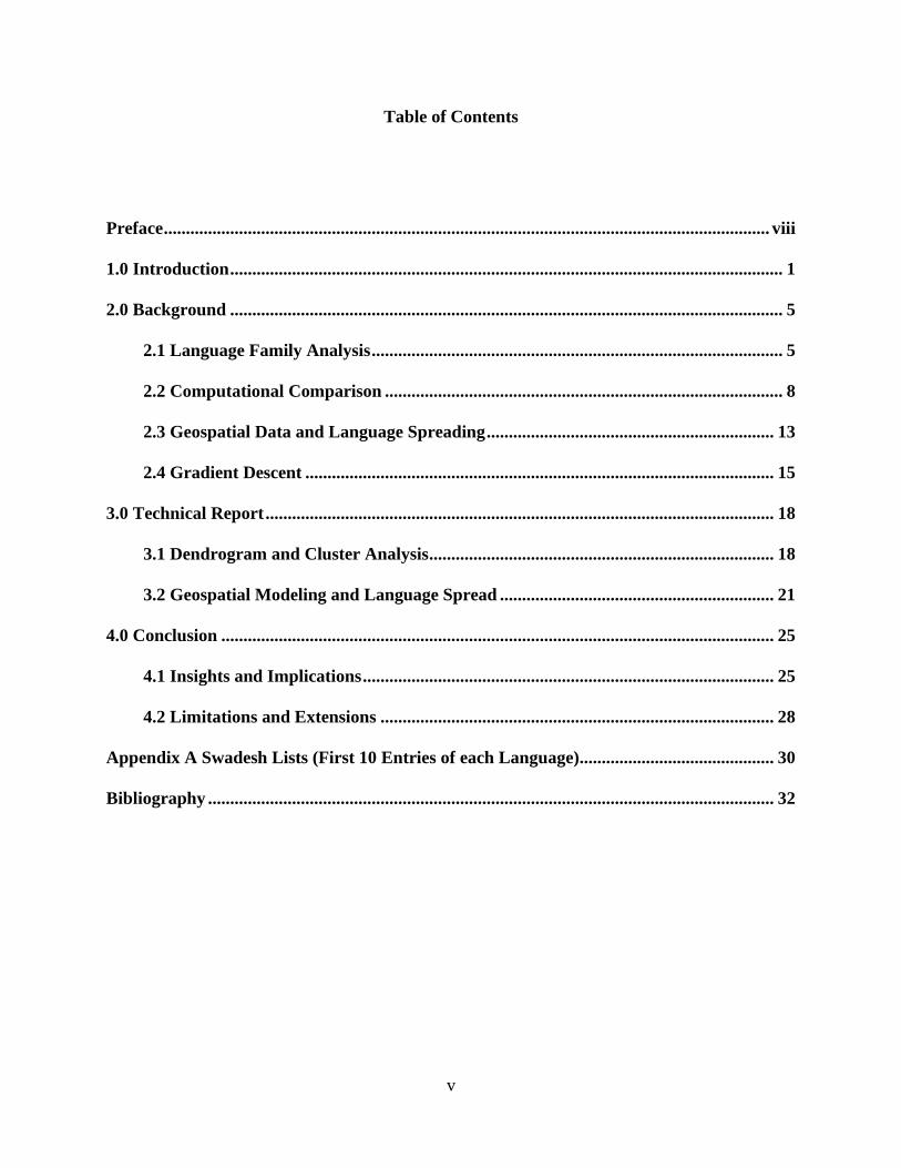
Table of Contents
Preface ......................................................................................................................................... viii
1.0 Introduction ............................................................................................................................. 1
2.0 Background ............................................................................................................................. 5
2.1 Language Family Analysis ............................................................................................. 5
2.2 Computational Comparison .......................................................................................... 8
2.3 Geospatial Data and Language Spreading ................................................................. 13
2.4 Gradient Descent .......................................................................................................... 15
3.0 Technical Report ................................................................................................................... 18
3.1 Dendrogram and Cluster Analysis .............................................................................. 18
3.2 Geospatial Modeling and Language Spread .............................................................. 21
4.0 Conclusion ............................................................................................................................. 25
4.1 Insights and Implications ............................................................................................. 25
4.2 Limitations and Extensions ......................................................................................... 28
Appendix A Swadesh Lists (First 10 Entries of each Language)............................................ 30
Bibliography ................................................................................................................................ 32
vi
List of Tables
Table 1. Examples of edit operations .......................................................................................... 9
Table 2. Example of minimum edit distance ............................................................................ 10
vii
List of Figures
Figure 1. An abbreviated family tree example of Indo-European Languages ........................ 7
Figure 2. An example surface, with the path of steepest descent shown in red. (Gillis 2006)
................................................................................................................................................... 16
Figure 3. A contour map of Figure 2, again with the path of steepest descent shown in red
(Gillis 2006) .............................................................................................................................. 16
Figure 4. The outputted family tree model using the clustering algorithm. .......................... 19
Figure 5. A already established family tree model for comparison (Gawron n.d.). ............. 19
Figure 6. Elevation map of the British Isles, light colors reflect higher elevation. ............... 22
Figure 7. A gradient flow imposed on the surface. .................................................................. 23
Figure 8. The movement of different initial conditions. .......................................................... 24
Figure 9. A dialectal map of British Isles (Jonathan 2015) ..................................................... 27
viii
Preface
This research is the culmination of extensive interviews about the facets of language and
computation and would not be possible with out the aide of many individuals. Thank you to
Professor Alan Juffs, Professor Melinda Fricke, and Professor Na-Rae Han for linguistic expertise
and fostering a sense curiosity. Thank you to the several mathematics instructors that have aided
this research both directly and indirectly. Thank you to the University of Pittsburgh for establishing
the BPhil program and supporting the students through it, particularly Mr. Jason Sepac, and Dean
David Hornyak.
Special gratitude is shown to those individuals willing to sit and member the defense
committee: Dr. Michael Schneier, Dr. Na-Rae Han, Dean Laura Dice.
The grandest thanks of all to Dr. Jeffrey Wheeler, who insisted he not be mentioned.
Without you, barely anything in my college career, particularly in research, would have been
accomplished.
This research focuses on languages and their spreading. In discussions “languages
spreading” will be taken to mean “people(s) who speak the language migrating over time”. That
is, the spread of language is synonymous with the spread of people.
1
1.0 Introduction
With many advancements in the world of computing, vastly different fields of study have
found advancements achievable with the use of computational methods. Researchers’ goals have
been given a new perspective on what is possible by leveraging the methodologies of computing
science. Further, some of these areas of study have seen the development of entirely novel sub-
fields due to the increase in application of technology. One of the greatest examples is linguistics.
Linguistics is the study of language in all of its facets: from the pronunciation of words
(phonetics), to how thoughts are constructed and articulated (morphology and syntax), to how it is
acquired and processed in the brain (psycho-linguistics). As mentioned, a new sub-area has
emerged applying the developments in computing: computational linguistics. We can see the new
technologies of this in everyday life. Speech-to-text, auto-correct applications, and even language-
learning software are results of this discipline that combines linguistics studies and practices with
computing methodologies to create these new products.
One of the areas of linguistics that has seen less involvement with computational methods
is phylogenetic analysis. This is the branch of linguistics that studies the way languages are
grouped and classified together in terms of language family. The study is predicated on the axiom
that languages change and evolve over time and have been doing so since their inception. The goal
of phylogenetic analysis is to figure out which languages are related to which in the phylogeny,
and further, to trace the history of languages and offer a complete anthology regarding their origin.
The classical approach in this area of linguistics, referred to also as historical or comparative
linguistics, has been a primarily qualitative examination of languages, referencing both temporal
(the natural chronological change of words) and the spatial (using certain words for certain objects
2
in one’s environment) aspect of language, as well as drawing upon the field of anthropology to
supplement information. This line of effort has long been treated as a purely human endeavor, but
this report will offer a computational approach to phylogenetic analysis.
The computational approach is key to this research: this study leverages developments in
the area of machine learning to gain insights into phylogenetic analysis. Machine learning is an
often-misunderstood term, synonymous with artificial intelligence. In the sense for this study,
machine learning will be the umbrella term which covers a range of computing methods that a
computer can employ to reveal insights into pattern recognition. It is these patterns that are being
sought in the area of phylogenetic analysis. That is, machine learning will be used to determine
patterns among language change.
The main machine learning methods that will be used in this study are clustering and
gradient descent. Clustering is an algorithm that allows a user to input a group of items, each
compared to each other by some metric of similarity and offers a hierarchical structure to them.
This means that, given a list of items and a way to realize how similar or different each item on
the list is to the other items, a computer can use a rigorous algorithm to generate groupings of the
items. The closer one item is grouped to another reflects a closeness in similarity. With this is
mind, it is a natural extension to see how this method would have applications in phylogenetic
analysis.
The second machine learning method that is used in this study is gradient descent. This is
a method that, when given a slope of a function, is able to find the direction that has the steepest
decline. The surface that is used to give an image of the function is the gradient, and any decline
from an original point is a descent, hence the term gradient descent. But when the focus is on a
real-world model of languages and how they spread across the Earth, capturing the spatial travel
3
of the people who speak a language will of course be important. In order to resolve this, geospatial
data is necessary. This study uses this data in order to inform the model of which direction
languages are likely to spread.
Crucial to the understanding of languages and the ways that they can evolve over time is
the concept of geospatial considerations. That is, where a people who speak a language are located
has a supreme bearing on its development and change. The way a language spreads cannot be
isolated from its geography. Given this, research here offers a way to incorporate at least some of
these considerations into a computational model of how language spreads. This is another natural
application of the gradient descent method discussed earlier.
This study will use elevation as a key informatic to influence a model of how languages
change. The natural formation of the area over which the way people who speak a language move
will of course dictate to some extent how isolated languages are and can decrease the likelihood
to evolve and change together. For example, the languages of the Indian sub-continent and present-
day China have long been separated by the Himalayan Mountains. Thus, comparative and
historical linguists can confidently conclude that there has been little interaction between the two
and the speakers of one were not able to travel to the speakers of another, due to this barrier.
Indeed, we see this principle’s effects when comparing different regions.
Geographic areas with mountainous terrain, such as the island of Papua New Guinea or the
Caucus Mountains have a dramatically high number of languages spoken in them, while vast
spaces of planes and rolling hills, such as Central and Norther Asia as well as parts of North Africa,
at different times through history, saw the spread of one single language or small language family
(Mongol and Arabic, respectively).
4
As discussed, there appears to be a natural connection between the classical methods of
language family analysis, and the spread of languages and the machine learning methods available
to researchers today. Thus, blending the two together is suggested to provide a fruitful line of effort
that will achieve results that can be considered to add to the understanding of these topics. This
research leverages machine learning algorithms to analyze the similarity of languages and
computationally group them into phylogeny, as well and provide a model for gaining insight into
how these languages would have spread.
As mentioned, there have been many advancements in computing leading to large leaps in,
and the formation of, computational linguistics. However, the focus has remained largely in things
regarding information technology, such as text-to-speech and autocorrect. And while these things
have been profitable, many large-scale endeavors, such as analyzing language families have been
left alone and inspected through classical methods. Linguists and anthropologists have worked
together to trace human languages over time and space seeking to piece together a historical
narrative of both people and language. These lines of effort have primarily focused on archeologic
and anthropologic excavations as well as the comparative method in linguistics. This research
offers not only new insights into these fields but expands upon new line of effort working in
tandem with already established methods to learn more about the very same narrative.
5
2.0 Background
As with any multidisciplinary study, this research draws upon broad concepts and research
from across multiple fields. This section will prove an organized background of previous methods
which served as both inspiration and foundation for this research project.
2.1 Language Family Analysis
The origin of historical linguistics, the sub-field focused on the history of languages
diverging from one another, traces its inception to the late 1700s (Campbell 2013), even though
the questions of language origin and similarities have been investigated through antiquity. Notable
names throughout history, such as Aristotle and the Brothers Grimm, have thought about language,
and indeed any person learning a new language or even coming across one would draw upon the
conventions of their mother tongue to expedite the learning process of a novel language. (A fact
leveraged by some language teachers (Saphiu 2016).)
This project focuses on the comparative linguistic branch of historical linguistics, the
discipline with the goal of comparing languages and ultimately placing them into families. This
article aims to provide computational evidence for comparing the languages of the Indo-European
language family. Indo-European is the term given to the languages which share a common
ancestor, termed Proto-Indo-European (PIE), and have thus spread from Iceland to Eastern India.
(Indeed, to the present day, the languages have spread farther than that, with the colonial era of
English and Spanish speakers, as well as present day human migration.) A few languages to
6
represent the scope of Indo-European languages are given here: Albanian, languages of ancient
Anatolia (Hittite), Armenian, Balto-Slavic Languages (Russian, Czech, Latvian,) Celtic languages
(Gaelic, Irish) , Germanic languages (German, English, Icelandic), Greek, Indo-Iranian languages
(Kurdish, Persian, Sanskrit, Urdu), Italic (Latin, Spanish, Italian)
While certainly not the first to make the claim, Sir William Jones, a judge from England,
presiding in India at the time is most widely credited with bringing the idea of Proto-Indo European
to the forefront of western language study (Patil 2003). Speaking English, Latin, and Greek, Jones
began to notice similarities between the ancient sacred language of India and the European
languages. Thus, a great leap forward in comparative linguistics was made.
Today, linguists have classified thousands of languages. But up until recently, these
classifications have been made using what is termed, the comparative method. This is the classical
method of determining the relationship of one language to another. While the precise and lengthy
details of this process are outside the scope of this background, a summary would typically follow
an outline such as:
1. Assemble words of same/similar meanings of the two languages
2. Establish the smallest possible correspondence
3. Determine if there is enough similarity to justify significant relationships.
Of course, a great deal of training and care must be taken to set out on tasks such as these.
The next step for comparative linguistics is to then take this process and determine a history
of language change, which typically manifests itself as a language family tree. (It is important to
note that there are of course competing theories of how languages change, but this research is
primarily focused on the family tree model, which is most prevalent.) This family tree reflects the
7
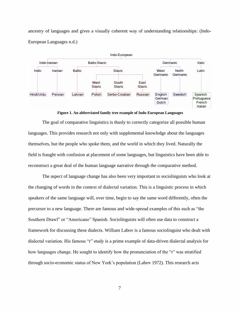
ancestry of languages and gives a visually coherent way of understanding relationships: (Indo-
European Languages n.d.)
The goal of comparative linguistics is thusly to correctly categorize all possible human
languages. This provides research not only with supplemental knowledge about the languages
themselves, but the people who spoke them, and the world in which they lived. Naturally the
field is fraught with confusion at placement of some languages, but linguistics have been able to
reconstruct a great deal of the human language narrative through the comparative method.
The aspect of language change has also been very important to sociolinguists who look at
the changing of words in the context of dialectal variation. This is a linguistic process in which
speakers of the same language will, over time, begin to say the same word differently, often the
precursor to a new language. There are famous and wide-spread examples of this such as “the
Southern Drawl” or “Americano” Spanish. Sociolinguists will often use data to construct a
framework for discussing these dialects. William Labov is a famous sociolinguist who dealt with
dialectal variation. His famous “r” study is a prime example of data-driven dialectal analysis for
how languages change. He sought to identify how the pronunciation of the “r” was stratified
through socio-economic status of New York’s population (Labov 1972). This research acts
Figure 1. An abbreviated family tree example of Indo-European Languages
8
similarly in trying to determine what factors may influence language change and how they be
able to be modeled.
2.2 Computational Comparison
The primary aim of this research is to offer a viable and reliable alternative to the discussed
comparative method. As computational efficiency grows, so does the scope of its application.
Researchers have already applied computational methods to linguistics, and this research presents
arguments for its continual use in historical and comparative aspects as well.
Thus far, many of these researchers have looked at comparative linguistics through the lens
of computation. Much of their work has had a heavy statistic lean to it, and incorporates a variety
of different strategies. Gerhard Jager of the University of Tubingen has written extensively on this
topic. In 2019, he published a comprehensive approach to using computational methods in
comparative analysis, going so far as to propose an entire workflow of the comparative method
(Jager 2019). This article also offers multiple case studies to demonstrate that validity of these
computational methods.
The key concepts that lay the foundation of these studies are phylogenetic relatedness and
Bayesian statistics. Jager published work establishing the support of predicted language families
with these statistical methods, that even the classical comparative method had struggled to
conclude definitively (Jager, Support for linguistic macrofamilies from weighted sequence
alignment 2015). This paper, among others, uses the ideas of posterior and prior probabilities,
trademarks of Bayesian statistics. Chang et al. also used computational methods to support claims
predicted by classical methods in linguistics. Their research provides evidence for the Proto-Indo-
9
European originating in the Kurgen Steppe (present day Ukraine), a long standing and popular
conjecture. It makes use of both the Bayesian statistics mentioned earlier and a probability
structure known as Markov chains to establish conclusions about the time of divergence based on
their phylogenetic relatedness (Will Chang 2015). Another important article which served as
inspiration for this research also drew upon Bayesian statistics when analyzing Semitic languages
(Arabic, Hebrew, Amharic, etc). These languages were not only analyzed with phylogenetic
analysis to establish genetic relationships, but considerations were given to inferred dispersal of
the people who spoke the language (Andrew Kitchen 2009). This indicates the importance of
geospatial data, and these projects indicate the fruitful application of computational methods in
comparative linguistics.
These projects all had a very high level of statistical basis for them. This present research
focuses on a new strategy for analyzing languages in a more discrete and non-parametric strategy.
This research employs edit distance as a way to establish similarity between two languages. Edit
distance is a measure of how much one word needs to be changed to become another. Words like
“cat” and “hat” have a small edit distance, while words like “cat” and “hippopotamus” have a
much larger one, as intuition would indicate. Formally, edit distance is often thought of as the
minimum number of edits (usually from a predetermined set of possible operations) that can be
done on a string of characters in order for one string to match another.
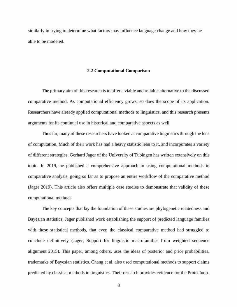
The most common forms of edits are insertion, deletion, swapping, and switching. These
are all intuitive with examples following:
Table 1. Examples of edit operations
Operation Pre-Edit Post-Edit
Insertion “sat” “stat”
10
Deletion “star” “star”
Swapping “sign” “sing”
Switching “crate” “grate”
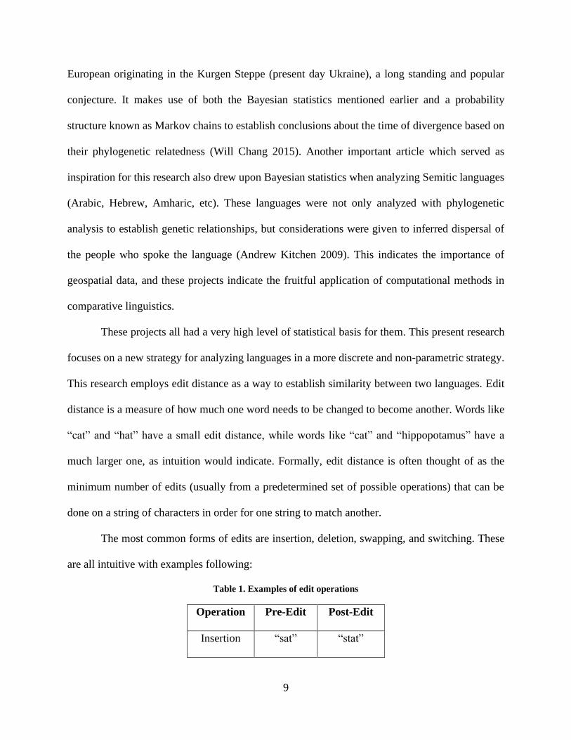
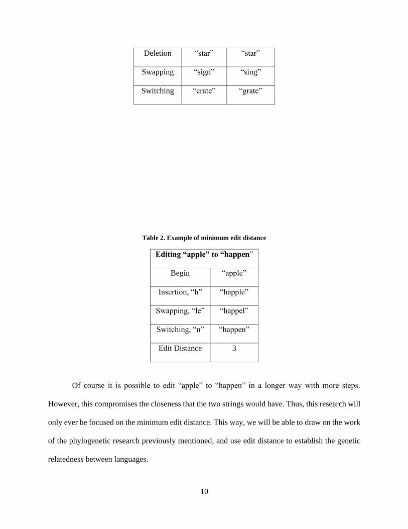
Table 2. Example of minimum edit distance
Editing “apple” to “happen”
Begin “apple”
Insertion, “h” “happle”
Swapping, “le” “happel”
Switching, “n” “happen”
Edit Distance 3
Of course it is possible to edit “apple” to “happen” in a longer way with more steps.
However, this compromises the closeness that the two strings would have. Thus, this research will
only ever be focused on the minimum edit distance. This way, we will be able to draw on the work
of the phylogenetic research previously mentioned, and use edit distance to establish the genetic
relatedness between languages.
11
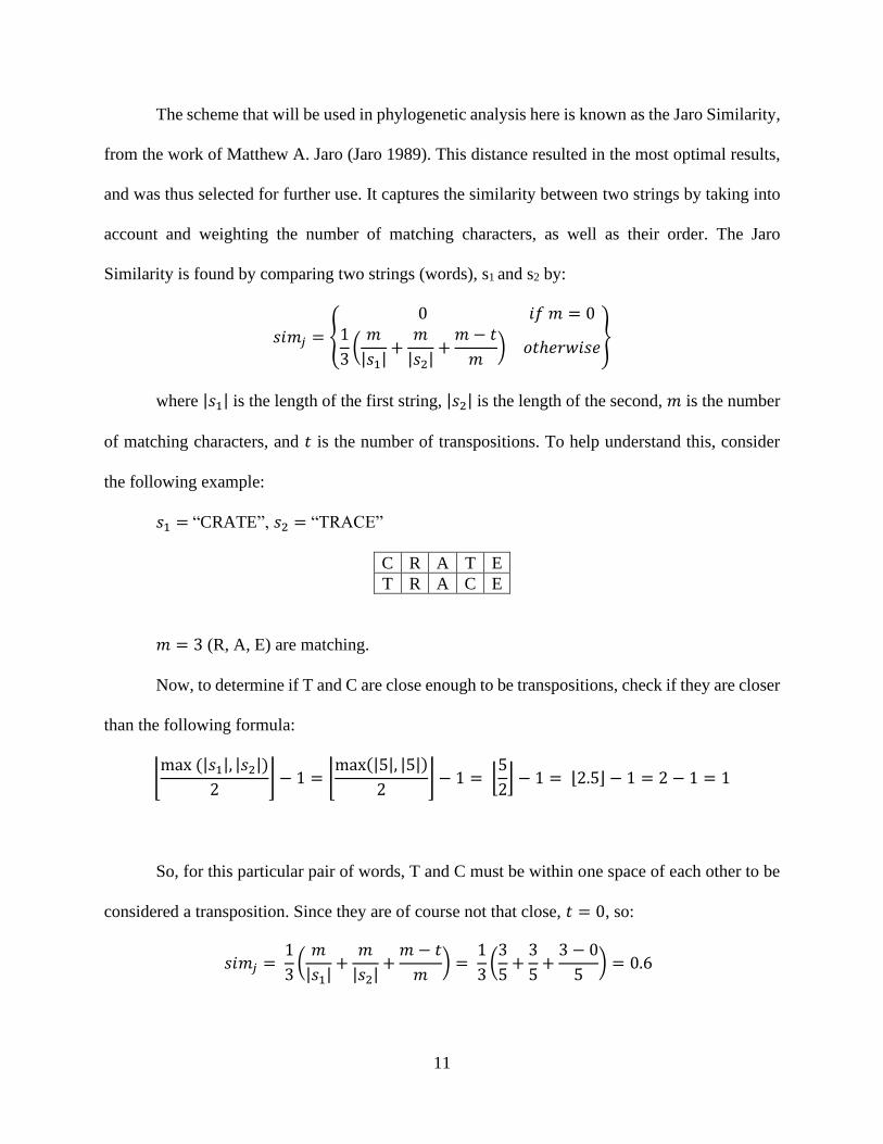
The scheme that will be used in phylogenetic analysis here is known as the Jaro Similarity,
from the work of Matthew A. Jaro (Jaro 1989). This distance resulted in the most optimal results,
and was thus selected for further use. It captures the similarity between two strings by taking into
account and weighting the number of matching characters, as well as their order. The Jaro
Similarity is found by comparing two strings (words), s1 and s2 by:
𝑠𝑖𝑚𝑗 = {
0 𝑖𝑓 𝑚 = 01
3(
𝑚
|𝑠1|+
𝑚
|𝑠2|+
𝑚 − 𝑡
𝑚) 𝑜𝑡ℎ𝑒𝑟𝑤𝑖𝑠𝑒
}
where |𝑠1| is the length of the first string, |𝑠2| is the length of the second, 𝑚 is the number
of matching characters, and 𝑡 is the number of transpositions. To help understand this, consider
the following example:
𝑠1 = “CRATE”, 𝑠2 = “TRACE”
C R A T E
T R A C E
𝑚 = 3 (R, A, E) are matching.
Now, to determine if T and C are close enough to be transpositions, check if they are closer
than the following formula:
⌊max (|𝑠1|, |𝑠2|)
2⌋ − 1 = ⌊
max(|5|, |5|)
2⌋ − 1 = ⌊
5
2⌋ − 1 = ⌊2.5⌋ − 1 = 2 − 1 = 1
So, for this particular pair of words, T and C must be within one space of each other to be
considered a transposition. Since they are of course not that close, 𝑡 = 0, so:
𝑠𝑖𝑚𝑗 = 1
3(
𝑚
|𝑠1|+
𝑚
|𝑠2|+
𝑚 − 𝑡
𝑚) =
1
3(
3
5+
3
5+
3 − 0
5) = 0.6
12
Thus, “CRATE” and “TRACE” have a Jaro Similarity of of 0.6. This with the range of 0
for no similarity, and 1 for an exact match.
To compare entire languages, of course, is much more involved. Instead of simply
comparing one word from each language, this research uses the field standard list of wards, known
as the Swadesh list. This is a formalized list of approximately 200-word meanings (depending on
version) that have been used by comparative linguistics to establish phylogeny. Published multiple
times in the 1950s, Morris Swadesh created a list of word meanings that are theoretically less likely
to change. This makes them prime candidates for establishing language families, as linguists are
less likely to get thrown off by language change phenomena.
The lists contain different classes of words, though ones that are crucial to everyday speech
and survival. Some deal with personhood, such as pronouns, and familial relationships. Others are
words for things found in the environment, such as trees and game. Still, other classes refer to
things such as numerals or abstract concepts. For this research Swadesh lists were gathered from
Wiktionary, an open source research with a vast array of Swadesh lists available (Wiktionary
2020). Validating the lists is outside the scope of this research, however, accurate results were able
to be obtained using them. An important note is that to ensure the integrity of linguistic processing,
all the lists were converted to a Roman alphabet, with the nearest orthographic equivalent. An
appendix with the entirety of the Swadesh List database is included for examination, as well as a
resource to continue this research.
Another important computational tool that will be used is clustering. Clustering is a basic
machine learning algorithm that takes a set of points, each with some notion of distance from one
another, and determines from them the optimal way to cluster. These clusters are then considered
to be groups with some form of relation to one another. These are then graphically represented in
13
a clustergram, also called a dendrogram, which reflects each level of clustering. One will note the
similarity between the dendrogram and the family tree model of language phylogenetics, making
an intuitive connection between the two.
2.3 Geospatial Data and Language Spreading
The other aim of this research is to add to the computational understanding the way
languages spread spatially across the surface of the earth. This is dictated, naturally, by the way
humans, the beings that carry a language move over time. Important to this research is the
deviation from the anthropological and archeological lines of effort, and the establishment of a
new conceptual framework for understanding human migration.
The feature that will be used in the model here is the idea of traversability. Even though
there are multiple definitions and specific parameters to measure traversability, here it will be
understood as a measure of the ease of a group of people to cross a space of land. Many factors
must be taken into account, as this is a very abstract concept. The University of Massachusetts,
with USDA Forest Service General Technical Report , and Oregon State University offer
FRAGSTATS as a way to understand and measure traversability (Kevin McGarigal 1994).
University of Massachusetts gives:
“Traversability index is computed at the cell level and then averaged across cells in the
focal patch. As a result, this metric requires substantial computations and may take considerable
time to compute for a large landscape. In addition, this metric requires the user to specify an
appropriate resistance matrix containing coefficients for each pairwise combination of patch types,
as well as a scaling factor that governs the size of the maximum least cost hull; that is, the size of
14
the area surrounding the focal cell that is accessible given minimum resistance. The size of
maximum least cost hull is based on a user-specified maximum distance or neighborhood distance.
Based on this distance, FRAGSTATS computes the “bank account” needed to achieve a circular
least cost hull with a radius equal to this distance.” (umass.edu/landeco n.d.)
While this research does not incorporate a resource bank, there are important features of
note here. The first is that traversability is calculated for individual areas of land. That is, the terrain
is considered to be a series of adjacent plots of arbitrary, but uniform, sizes such that each has its
own measure of traversability. As the research today is concerned with Indo-European languages
at large, data degrading minimum least cost hull and resource data is not available. To maintain a
notion of traversability, this research use elevation to consider the way languages may move.
This does tend to reflect observations seen in the real world. As mentioned, flat plains
ecosystems, such as the Mongolian Empire or North African coastal plains see a high level of
uniformity throughout, while mountainous regions such as Papua New Guinea and the Caucus
Regions have a great deal of language diversity. The reasons for this are often cited to be the
terrain; the fact the mountains and valleys create pockets for languages to change independent of
one another is the reason we see such stark contrasts. Thus, elevation will be the primary measure
of the traversability for this research. For this research, elevation data was taken from the open
source site GeoNames (GeoNames 2020)
15
2.4 Gradient Descent
The notion of traversability as a function of elevation gives way to a natural method in
machine learning known as gradient descent. This is a technique that is found in the area of convex
optimization. Developed by the famed mathematician Cauchy in 1847 (Lemaréchal 2012), it is
employed to find the minimum value of a 2- or 3-dimenstional function, by using the derivative,
which in 3 dimensions is called a gradient, to determine minimum values. The algorithm works by
assuming that the direction which has the steepest descent is the direction that needs to be taken in
order to find the minimum values. The algorithm terminates when the rate of improvement
becomes negligible; that is when moving around the surface no longer results in a significant
enough decrease in the value of the function, gradient descent end. This suggests that the process
is not guaranteed to give an exact value, nor even a global minimum.
But, what is important here is not necessarily the minimum value that is achieved, but the
path that gradient descent prescribes in its solution finding process. When taking the steps across
the surface, and finding the gradient along it, the process records the path taken, the path of steepest
descent. This is what will be useful in the research here. Considering the surface of the Earth to be
like a function, we can consider that this path of steepest descent can be considered the path of
least resistance for a group of people to take (ie. Not climbing over mountains), which in turn could
be considered to be the route that has the highest degree of traversability. Thus, the use of gradient
descent is a natural addition to this research, fitting in well with considerations for traversability.
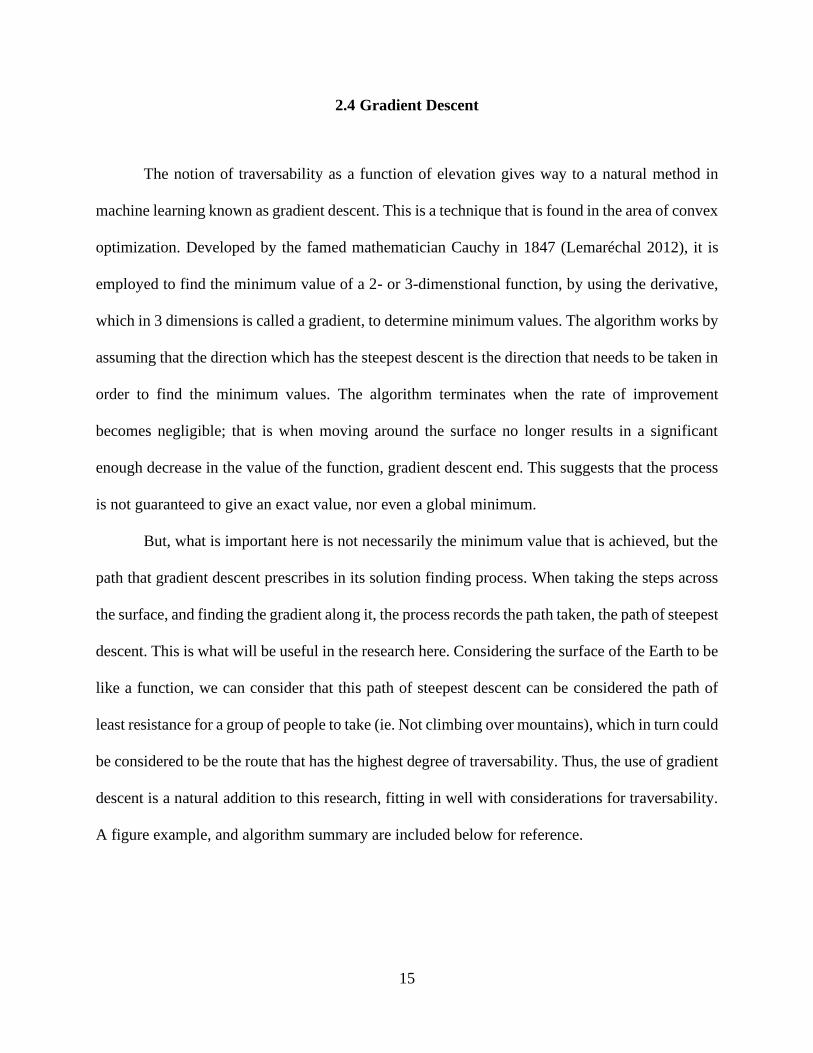
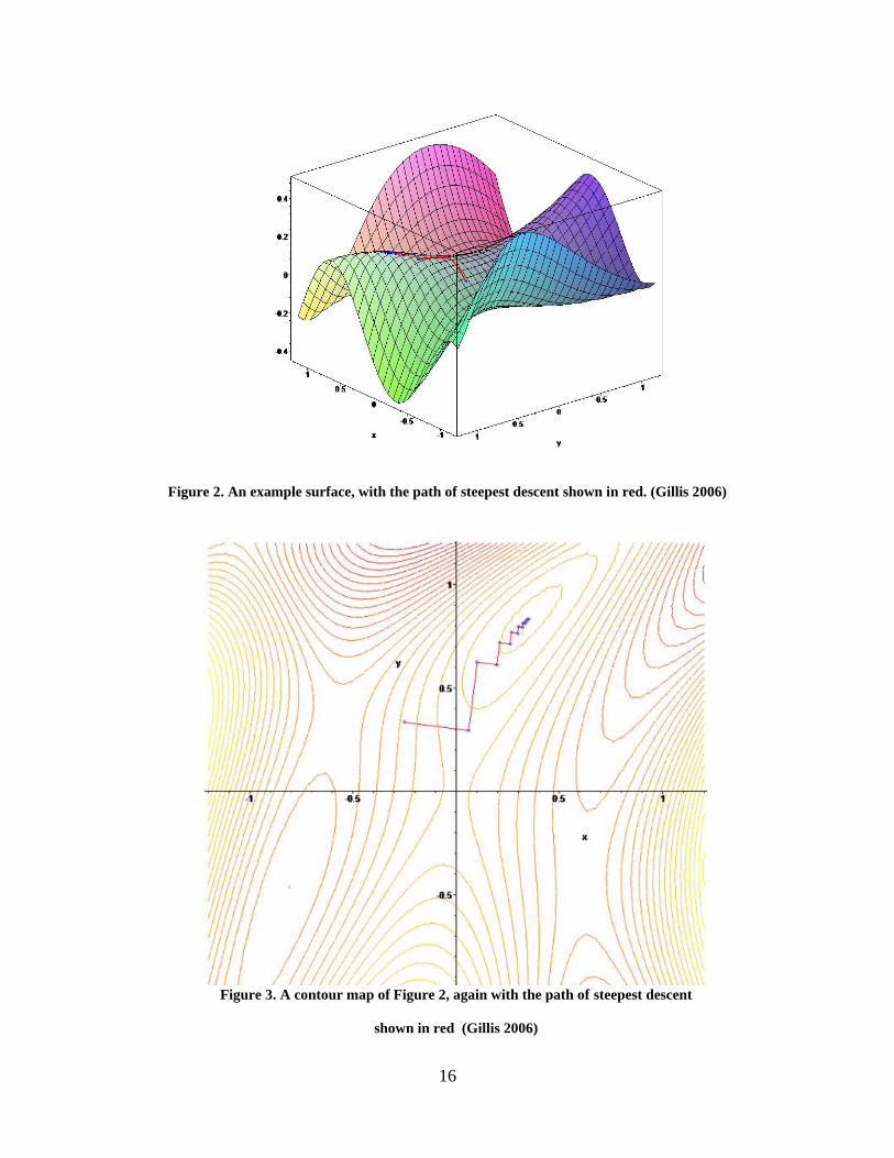
A figure example, and algorithm summary are included below for reference.
16
Figure 2. An example surface, with the path of steepest descent shown in red. (Gillis 2006)
Figure 3. A contour map of Figure 2, again with the path of steepest descent
shown in red (Gillis 2006)
17
Specifically, what this research will implement is an array of starting points. These will be
representative of different starting points that groups of humans, the beings that carry language.
Then, the gradient flow algorithm will be allowed to ensue, and these objects, the people, will be,
predictably, find their local minima. This will of course exclude a lot of typical movement of
people and emphasize things such as coastward movement, but the elevation will serve as a basis
on which to expand.
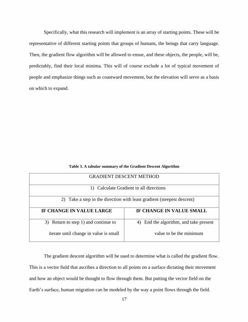
Table 3. A tabular summary of the Gradient Descent Algorithm
GRADIENT DESCENT METHOD
1) Calculate Gradient in all directions
2) Take a step in the direction with least gradient (steepest descent)
IF CHANGE IN VALUE LARGE IF CHANGE IN VALUE SMALL
3) Return to step 1) and continue to
iterate until change in value is small
4) End the algorithm, and take present
value to be the minimum
The gradient descent algorithm will be used to determine what is called the gradient flow.
This is a vector field that ascribes a direction to all points on a surface dictating their movement
and how an object would be thought to flow through them. But putting the vector field on the
Earth’s surface, human migration can be modeled by the way a point flows through the field.
18
3.0 Technical Report
This section is focused on a summary and technical report of what was accomplished in
this research. Contained here is a discussion of the methods used, as well as outputs from various
portions of code. The software used is the open source software R Statistical Programming, along
with various packages.
3.1 Dendrogram and Cluster Analysis
The first step in the program is the phylogenetic analysis. To create the desired graphics,
the Swadesh lists were compiled and aggregated. To ensure the best possible results, the textual
data had to be cleaned: all white space removed and characterized Romanized. Then, a distance
matrix was created. A distance matrix is a data structure which allows hierarchical clustering to
take place. This clustering is what gives rise to the family tree model as explained previously. The
clusters can be considered to be the language family, and in order to see the clusters, similarity
must be established. To do this, the Jaro Similarity was used.
The result of this is a similarity matrix. This is a data structure that contains the average
similarity of one language to another, by finding the mean similarity of each that is paired on the
Swadesh list. Conceptually, each word in the Swadesh lists for the language has its own similarity
matrix, and all of these matrices are averaged to determine the overall similarity. This final matrix
was then put through the clustering algorithm to create the clusters which would ultimately result
in the following dendrogram:
19
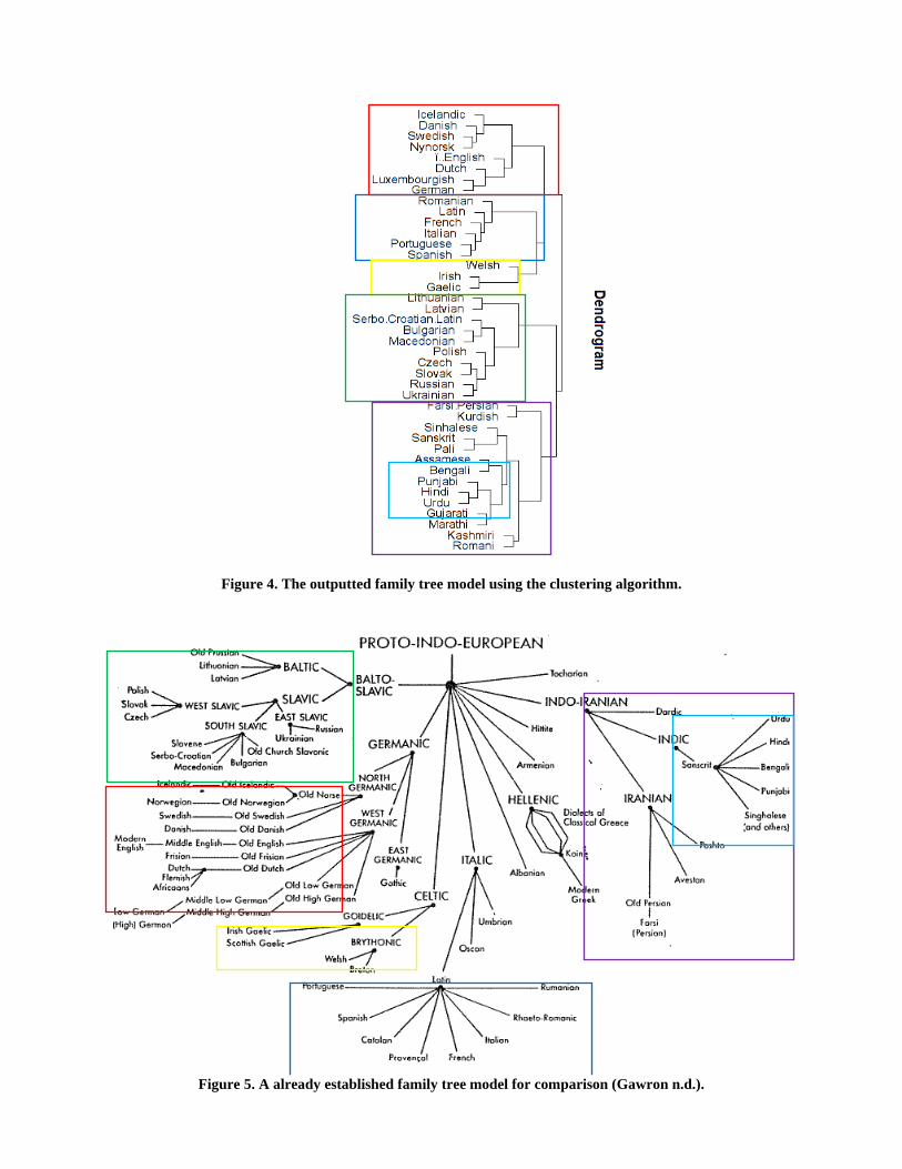
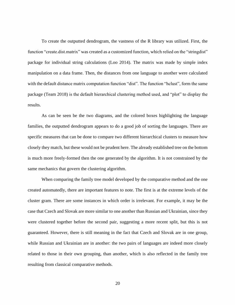
Figure 4. The outputted family tree model using the clustering algorithm.
Figure 5. A already established family tree model for comparison (Gawron n.d.).
20
To create the outputted dendrogram, the vastness of the R library was utilized. First, the
function “create.dist.matrix” was created as a customized function, which relied on the “stringdist”
package for individual string calculations (Loo 2014). The matrix was made by simple index
manipulation on a data frame. Then, the distances from one language to another were calculated
with the default distance matrix computation function “dist”. The function “hclust”, form the same
package (Team 2018) is the default hierarchical clustering method used, and “plot” to display the
results.
As can be seen be the two diagrams, and the colored boxes highlighting the language
families, the outputted dendrogram appears to do a good job of sorting the languages. There are
specific measures that can be done to compare two different hierarchical clusters to measure how
closely they match, but these would not be prudent here. The already established tree on the bottom
is much more freely-formed then the one generated by the algorithm. It is not constrained by the
same mechanics that govern the clustering algorithm.
When comparing the family tree model developed by the comparative method and the one
created automatedly, there are important features to note. The first is at the extreme levels of the
cluster gram. There are some instances in which order is irrelevant. For example, it may be the
case that Czech and Slovak are more similar to one another than Russian and Ukrainian, since they
were clustered together before the second pair, suggesting a more recent split, but this is not
guaranteed. However, there is still meaning in the fact that Czech and Slovak are in one group,
while Russian and Ukrainian are in another: the two pairs of languages are indeed more closely
related to those in their own grouping, than another, which is also reflected in the family tree
resulting from classical comparative methods.
21
The second caveat is at the higher levels of clustering. Even though the Slavic languages
are predicted to be more closely related to the Indo-Iranian languages than to the Germanic
languages, one should be hesitant to affirm such strong claims. But, the notion that Indic languages
are a subset of Indo-Iranian languages is of course true. A qualitative examination of these outputs
does suggest validity for both the clustering method to modeling how languages spread, and the
use of the Jaro Distance to determining word similarity.
It is not abundantly clear as to why the Jaro distance appeared to output the highest
similarity between the computational and comparative methods. This may be considered a “black-
box” programming method. However, reasons for this may include the fact that the Jaro similarity
has much more a sliding scale approach. While elementary methods simply count steps, the Jaro
distance considers things such as position distance between letters, and how much the characters
of one string match another. With much more robust detection, the Jaro similarity is suggested to
be useful for this line of effort.
3.2 Geospatial Modeling and Language Spread
As discussed, the second main focus of this research is to find a way to computationally
understand how people could move through the environment. The program here will be utilizing
gradient descent to capture the movement of people. To do this, gradient descent algorithms will
be conducted across multiple areas to construct a gradient flow, which will serve as a reference for
how an group of people may flow through the environment. First, a geospatial map was constructed
22
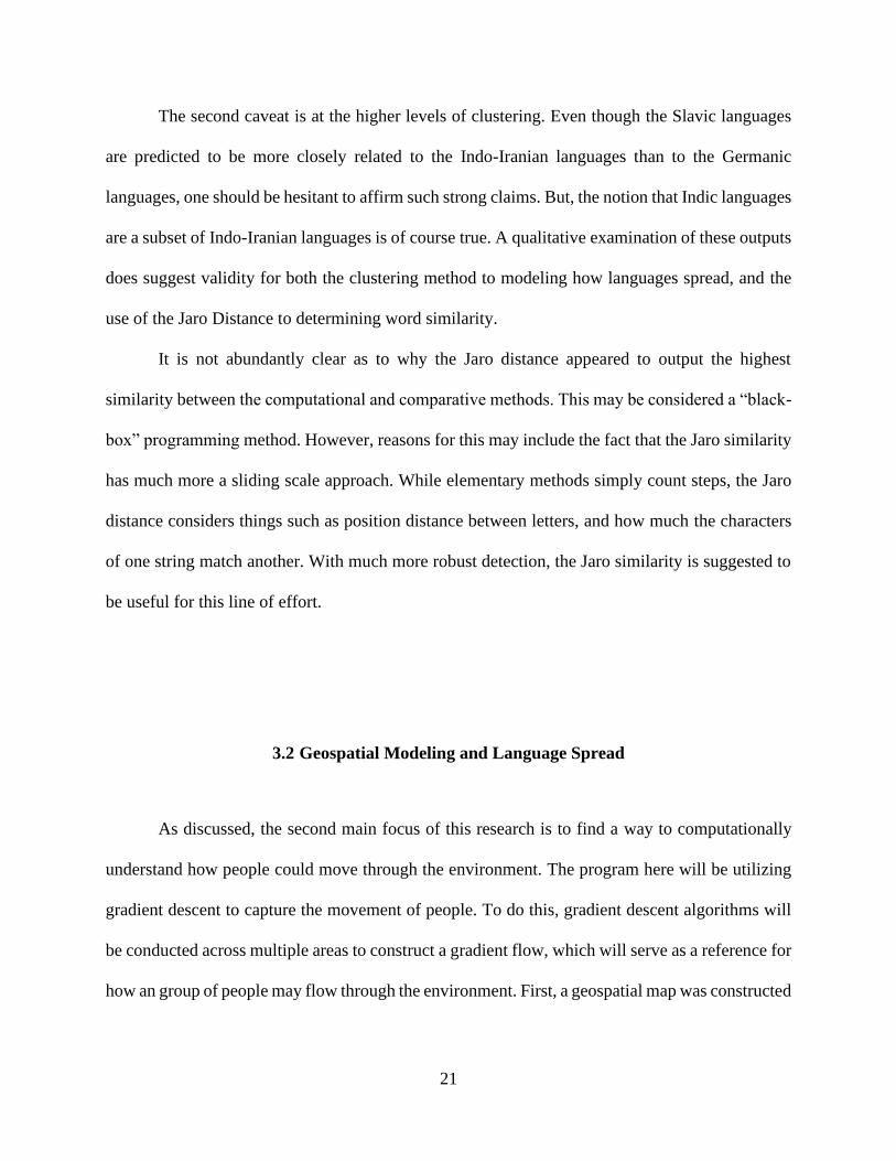
in R, and then from GeoNames.org, elevation data was imported for each of a series of coordinates,
relating the positions on a map. A example is given below:
Figure 6. Elevation map of the British Isles, light colors reflect higher elevation.
This is an elevation map of the British Isles, along with northwestern France. Clearly
visible are the Scottish Highlands, the English Lowlands, along with the mountainous regions in
Wales. To construct high resolution elevation plots, especially for wider areas, requires higher
levels of computing than is capable for research of this scope.
However, proceeding with the steps reveals interesting results. By using gradient descent
and creating a gradient flow, or a vector field, we find a model of the world’s surface for predicting
the movement of people:
23
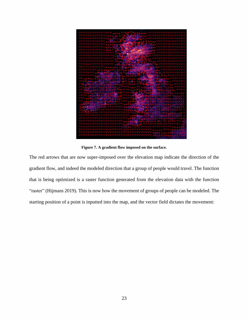
Figure 7. A gradient flow imposed on the surface.
The red arrows that are now super-imposed over the elevation map indicate the direction of the
gradient flow, and indeed the modeled direction that a group of people would travel. The function
that is being optimized is a raster function generated from the elevation data with the function
“raster” (Hijmans 2019). This is now how the movement of groups of people can be modeled. The
starting position of a point is inputted into the map, and the vector field dictates the movement:
24
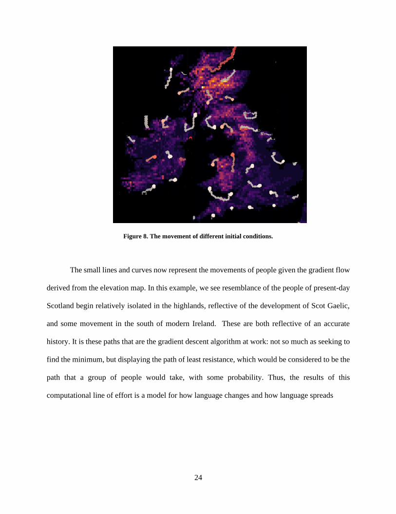
Figure 8. The movement of different initial conditions.
The small lines and curves now represent the movements of people given the gradient flow
derived from the elevation map. In this example, we see resemblance of the people of present-day
Scotland begin relatively isolated in the highlands, reflective of the development of Scot Gaelic,
and some movement in the south of modern Ireland. These are both reflective of an accurate
history. It is these paths that are the gradient descent algorithm at work: not so much as seeking to
find the minimum, but displaying the path of least resistance, which would be considered to be the
path that a group of people would take, with some probability. Thus, the results of this
computational line of effort is a model for how language changes and how language spreads
25
4.0 Conclusion
Thys, what this research is able to present is two-fold. The first is an argument for the
validity and usefulness of the Jaro distance for similarity, and the clustering algorithm for structure.
These are two powerful computational tools that when combined, offer results closely mirroring
those of already established methods, suggesting that the line of effort in computational studies
offer useful results. The second insight offered is a basis for a computational model of the world.
While only elevation was considered, the gradient approach was shown, regarding how to model
the spread of people throughout the world.
Here will be the discussion of the results presented previously. Also included are
implications from this research as well as limitations of what was able to be conducted. Further
extensions are offered, some of which are underway now.
4.1 Insights and Implications
First, considering the phylogenetic aspects of the project, what was shown was a successful
method for classifying languages into families based on their Swadesh lists. What can be learned
from this is twofold: first, that the metric used, the Jaro similarity, is able to, in some capacity,
capture language change. This implies that a model of language change that uses the Jaro similarity
to define edit distance may be useful and accurate. The second implication from this line of effort
is the hypotheses that may be conjectured from output. Particularly if more data is used,
anthropologists, linguists and computer scientists may be able to begin to make conjecture of a
26
farther-reaching nature. The ideas of large language families, branching over multiple major
classifications of Indo-European languages have swirled around the linguistic community for
decades, but have failed to gain much traction. With this advancement in phylogenetic analysis,
the greater pattern recognition of computers can be used to make conjectures of these macro-
families.
Secondly, concerning the modeling of the Earth’s surface, while a truly accurate model
may be very elusive as there is a great abundance of variable to consider, the spread of language
may indeed be able to be based on the spread of people still. This presents the possibility that
geospatial data can yield important insights into the spread of language. Here, elevation was used,
and was seen to have some insights into the way language travels. It is seen in the example that
there are some similarities between real-world history and the computational line of effort shown
here. Perhaps even further conjectures can be made based on what is computationally available.
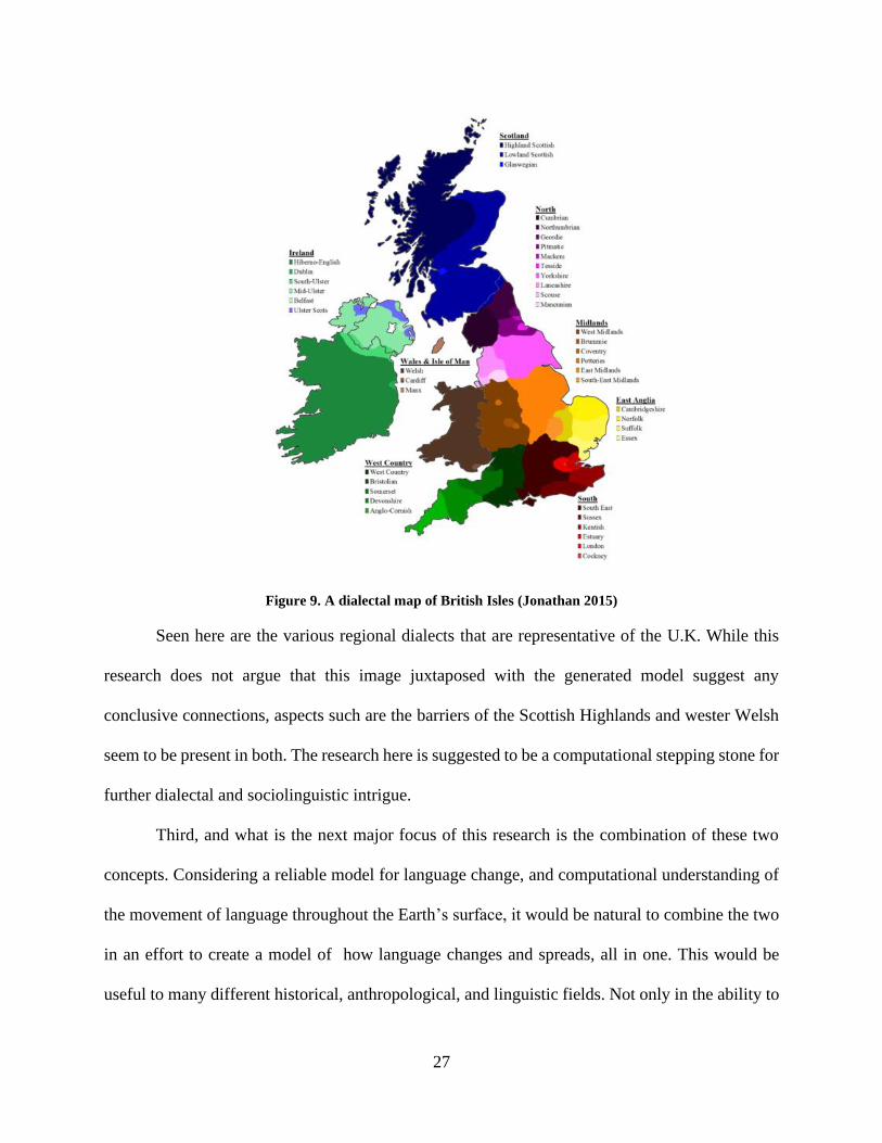
The map of Britain containing the representation of the movements of people across the
surface does offer some interesting possibilities itself. Consider the following figure of the
dialectal map of the same region:
27
Figure 9. A dialectal map of British Isles (Jonathan 2015)
Seen here are the various regional dialects that are representative of the U.K. While this
research does not argue that this image juxtaposed with the generated model suggest any
conclusive connections, aspects such are the barriers of the Scottish Highlands and wester Welsh
seem to be present in both. The research here is suggested to be a computational stepping stone for
further dialectal and sociolinguistic intrigue.
Third, and what is the next major focus of this research is the combination of these two
concepts. Considering a reliable model for language change, and computational understanding of
the movement of language throughout the Earth’s surface, it would be natural to combine the two
in an effort to create a model of how language changes and spreads, all in one. This would be
useful to many different historical, anthropological, and linguistic fields. Not only in the ability to
28
confirm theories through a new line of effort, diverse from the previous ones, but to offer new and
further reaching explanations and hypotheses.
4.2 Limitations and Extensions
As with any modeling project, limitations, often in the form of assumptions, are required
to have a functional output, but can result in lower fidelity results. The first limitation appears in
the limitation of computational capabilities. As with any big computational undertaking,
limitations will occur. For this project, in particular, the incorporation of elevation data presented
a challenge. Covering the entirety of the over 8,000 km distance that the Indo-European Language
Family has spread with fine grain elevation data requires a significant amount of time to retrieve
the data from the online source.
Another important factor regarding the geospatial data is other factors, such as habitability.
Consider for example things such as climate and agriculture potential. These things have such a
large bearing on human migration that a model would much less useful without them. Consider
the planes of Siberia. Even though the model here would say that there would be high rates of
language spreading, history would disagree, as the region is difficult to inhabit due to a hostile
climate.
Another real-world consideration that is left out of the model is the role of empires. Vast
empires and kingdoms are often the reason that one language succeeds over another. This is a
smaller subset of a larger considerations, that of competition. Competition modeling is a rich field,
which is often applied to languages. Incorporating these into the model will produce higher fidelity
results.
29
Concerning the phylogenetic clustering methods, departure from orthographic
representation of words can be used to determine the way language changes over time. For this
research, the Romanized versions of these words was used because of data availability and the fact
that orthography can reveal relations. Work has already been conducted to use the International
Phonetic Alphabet as a way to transcribe the Swadesh lists, so that differences in script and spelling
will not hinder this method. While there is still validity in what was done here, as the results appear
to match already established methods, one would want to use the purest transcription possible
(IPA) to conjecture about specific sound changes.
Perhaps the most crucial extension for this project is the combination of modeling language
change and language spreading. The two lines of the effort can be combined together to gain
information about the way languages change. What is important about this is the possibilities of
simulations. These simulations which can span centuries, can help determine the correct past,
because a model which incorporates a lot of data, can simulate many possibilities, and the one that
results in the most accuracy to real-world occurrences, may offer insight as to how languages have
truly changed and evolved over time.
30
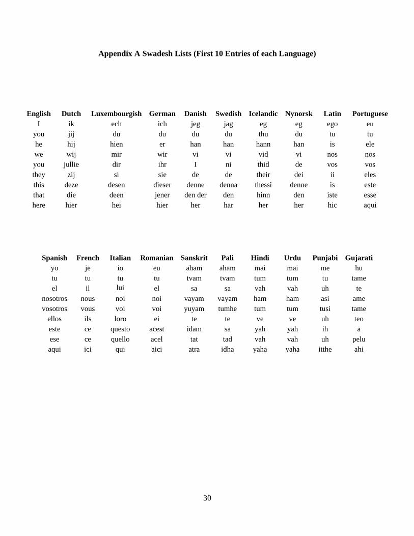
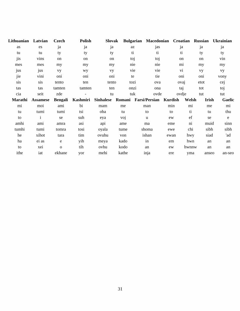
Appendix A Swadesh Lists (First 10 Entries of each Language)
English Dutch Luxembourgish German Danish Swedish Icelandic Nynorsk Latin Portuguese
I ik ech ich jeg jag eg eg ego eu
you jij du du du du thu du tu tu
he hij hien er han han hann han is ele
we wij mir wir vi vi vid vi nos nos
you jullie dir ihr I ni thid de vos vos
they zij si sie de de their dei ii eles
this deze desen dieser denne denna thessi denne is este
that die deen jener den der den hinn den iste esse
here hier hei hier her har her her hic aqui
Spanish French Italian Romanian Sanskrit Pali Hindi Urdu Punjabi Gujarati
yo je io eu aham aham mai mai me hu
tu tu tu tu tvam tvam tum tum tu tame
el il lui el sa sa vah vah uh te
nosotros nous noi noi vayam vayam ham ham asi ame
vosotros vous voi voi yuyam tumhe tum tum tusi tame
ellos ils loro ei te te ve ve uh teo
este ce questo acest idam sa yah yah ih a
ese ce quello acel tat tad vah vah uh pelu
aqui ici qui aici atra idha yaha yaha itthe ahi
31
Marathi Assamese Bengali Kashmiri Sinhalese Romani Farsi/Persian Kurdish Welsh Irish Gaelic
mi moi ami bi mam me man min mi me mi
tu tumi tumi tsi oba tu to to ti tu thu
to i se suh eya voj u ew ef se e
amhi ami amra asi api ame ma eme ni muid sinn
tumhi tumi tomra tosi oyala tume shoma ewe chi sibh sibh
he xihot tara tim ovuhu von ishan ewan hwy siad 'ad
ha ei as e yih meya kado in em hwn an an
to xei o tih ovhu kodo an ew hwnnw an an
ithe iat ekhane yor mehi kathe inja ere yma anseo an-seo
Lithuanian Latvian Czech Polish Slovak Bulgarian Macedonian Croatian Russian Ukrainian
as es ja ja ja az jas ja ja ja
tu tu ty ty ty ti ti ti ty ty
jis vins on on on toj toj on on vin
mes mes my my my nie nie mi my my
jus jus vy wy vy vie vie vi vy vy
jie vini oni oni oni te tie oni oni vony
sis sis tento ten tento tozi ova ovaj etot cej
tas tas tamten tamten ten onzi ona taj tot toj
cia seit zde - tu tuk ovde ovdje tut tut
32
Bibliography
Andrew Kitchen, Christopher Ehret, Shiferaw Assefa, Connie J. Mulligan. 2009. "Bayesian
phylogenetic analysis of Semetic languages identifies an Early Bronze age origin of
Semetic in the Near East." Proceedings of the Royal Society B 2703-2710.
Campbell, Lyle. 2013. Historical Linguistics: An Introduction 3rd Edition. Cambridge, MA: MIT
Press.
Gawron, Jean Mark. n.d. Language Change. Accessed March 2020.
https://gawron.sdsu.edu/fundamentals/course_core/lectures/historical/historical.htm.
2020. GeoNames. April. Accessed February - March 2020. geonames.org.
Gillis, Joris. 2006. The gradient descent algorithmn in action.
Hijmans, Robert J. 2019. "raster: Geographic Data." R package version 3.0-7. https://CRAN.R-
project.org/package=raster.
n.d. "Indo-European Languages." Essential Humanities. Accessed April 2, 2020.
http://www.essential-humanities.net/history-supplementary/indo-european-languages/.
Jager, Gerhard. 2019. "Computational historical linguistics." Theoretical Linguistics 151-182.
Jager, Gerhard. 2015. "Support for linguistic macrofamilies from weighted sequence alignment."
Proceedings of the National Academy of Sciences 12752-12757.
Jaro, M. A. 1989. "Advances in record linkage methodology as applied to the 1985 census of
Tampa Florida." Journal of the American Statistical Association 414-420.
Jonathan. 2015. Algotopia.net. June 12. Accessed April 16, 2020.
https://www.anglotopia.net/british-identity/english-language/english-language-map-of-
the-various-accents-in-the-british-isles-british-accent-map/.
33
Kevin McGarigal, Barbara J. Marks. 1994. FRAGSTATS: Spatial Pattern Analysis Program for
Quantifying Landscape Structure. Oregon State University.
Labov, William. 1972. "The Social Stratification of (r) in New York City Department Store."
Sociolinguistic Patterns 43-54.
Lemaréchal, C. 2012. "Cauchy and the Gradient Method." Math Extra 251-254.
Loo, M.P.J. van der. 2014. "The stringdist package for approximate string matching." R 111-122.
Patil, Narendranath B. 2003. The Variegated Plumage: Encounters with Indian Philosophy : a
Commemoration Volume in Honour of Pandit Jankinath Kaul "Kamal". Delhi: Motilal
Banarsidass Publications.
Saphiu, Dr. Isa. 2016. "Using Native Language in ESL Classroom." IJ-ELTS: International
Journal of English Language & Translation Studies 243-248.
Team, R Core. 2018. "R: A language and environment for statistical computing." Vienna: R
Foundation for Statistical Computing. https://www.R-project.org/.
n.d. umass.edu/landeco. Accessed February 2020.
http://www.umass.edu/landeco/research/fragstats/documents/Metrics/Connectivity%20M
etrics/Metrics/C123%20-%20TRAVERSE.htm.
Wiktionary. 2020. "Appendix: Swadish Lists." Wikipedia. March 30. Accessed January-March
2020. https://en.wiktionary.org/wiki/Appendix:Swadesh_lists.
Will Chang, Chundra Cathcart, David Hall, Andrew Garrett. 2015. "Ancestry-constrained
phylogenetic analysis supports the Indo-European steppe hypothesis." Language 194-244.

34