U N I V E R S I T Y O F B A L A M A N D ELEN 443
PROJECT 2
BPSK, FSK, AND ASK COMMUNICATION SYSTEMS
DIGITAL COMMINCATIOM
SUBMITTED BY RAYANE KHODOR, REWA SHOUJAA,
HAROUT GHAZARIAN & JAD ARAYJI
SUBMITTED TO DR. JIHAD DABA
PART I - PBSK SIMULATOR
THEORRETICAL APPROACHES AND MODELING
In phase shift keying (PSK), the phase of a carrier is changed according to the
modulating waveform which is a digital signal. Binary Phase Shift Keying (BPSK) is
a type of phase modulation using 2 distinct carrier phases to signal ones and zeros.
BPSK is the simplest form of PSK. This modulation is the most robust of all the PSKs
since it takes serious distortion to make the demodulator reach an incorrect decision
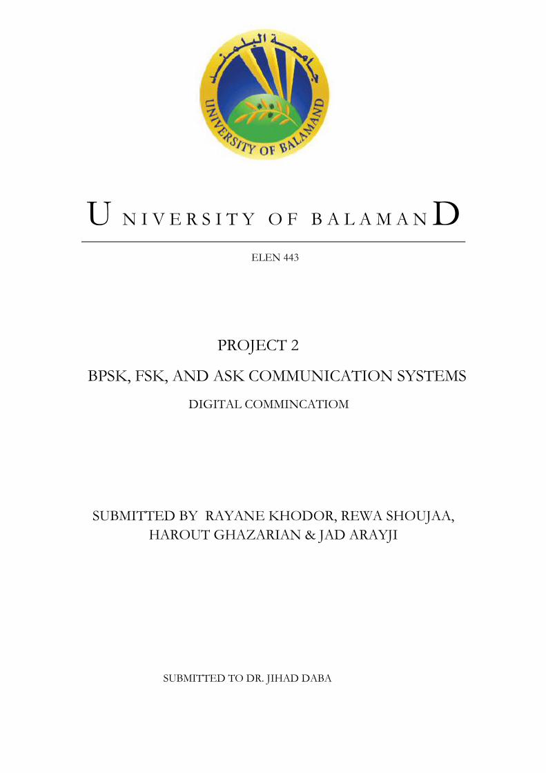
In BPSK, the transmitted signal is a sinusoid of fixed amplitude. It has one fixed
phase when the data is at one level and when the data is at the other level, phase is
different by 180 degree. A Binary Phase Shift Keying (BPSK) signal can be defined
as
Si(t) = (-1)i+1
Ac cos(2πfct)
Where Ac represents the peak value of sinusoidal carrier, b(t) = +1 or -1, fc is the
carrier frequency, and T is the bit duration.
The Generator Structure:
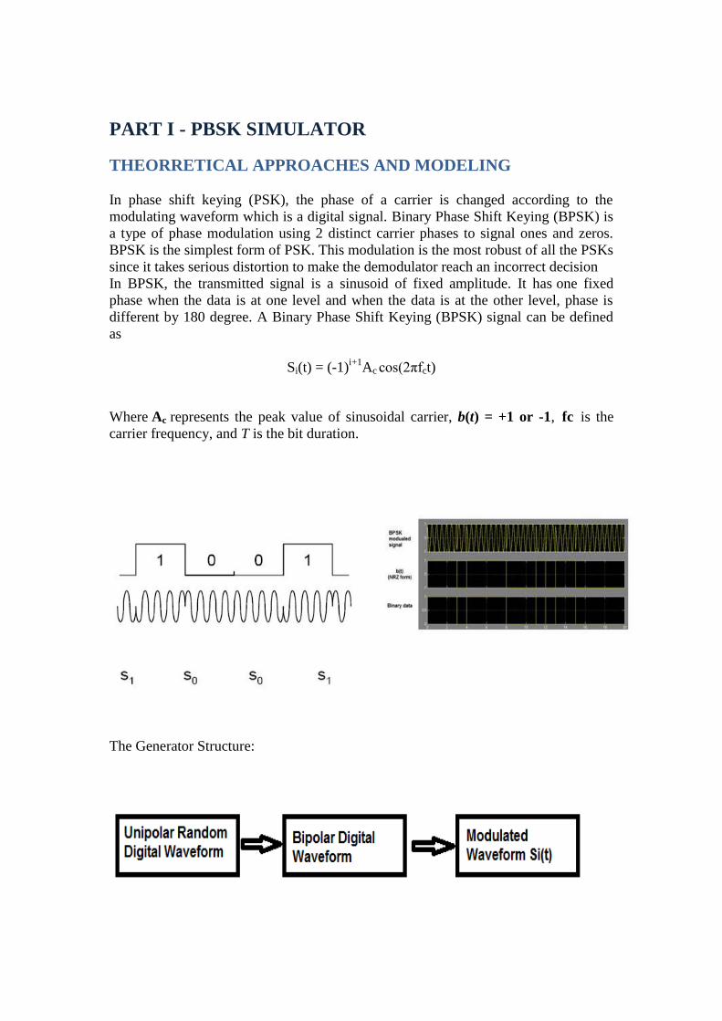
The Receiver Structure:
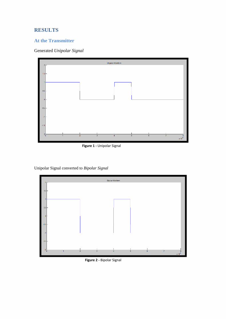
We generated a random unipolar signal with equally probable binary symbols. Then
we converted it into a bipolar digital waveform and finally we generated the
modulated signal si(t) using BPSK. At the receiver, we received a noisy signal with a
white Gaussian noise so a match filter is used for maximizing the signal to noise
ratio (SNR) in the presence of additive stochastic noise. Finally the signal is sampled
at the bit period Tb and a decision is made on whether a bit is 1 or 0 depending if the
signal is more or less than the computed threshold.
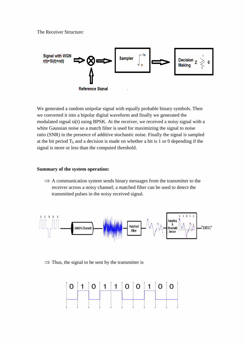
Summary of the system operation:
A communication system sends binary messages from the transmitter to the
receiver across a noisy channel; a matched filter can be used to detect the
transmitted pulses in the noisy received signal.
Thus, the signal to be sent by the transmitter is
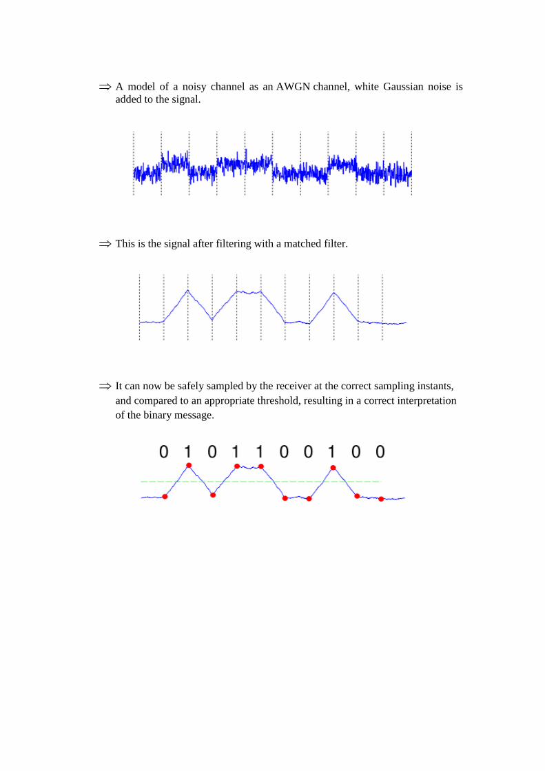
A model of a noisy channel as an AWGN channel, white Gaussian noise is
added to the signal.
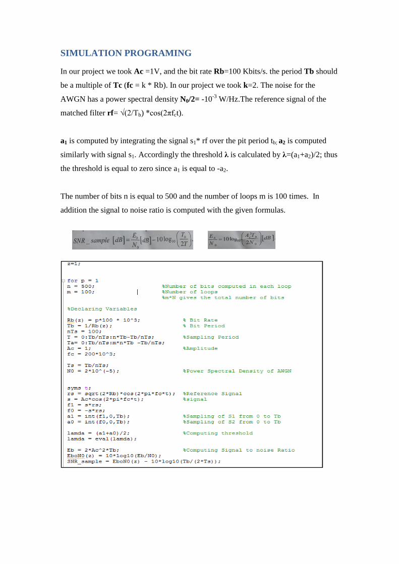
This is the signal after filtering with a matched filter.
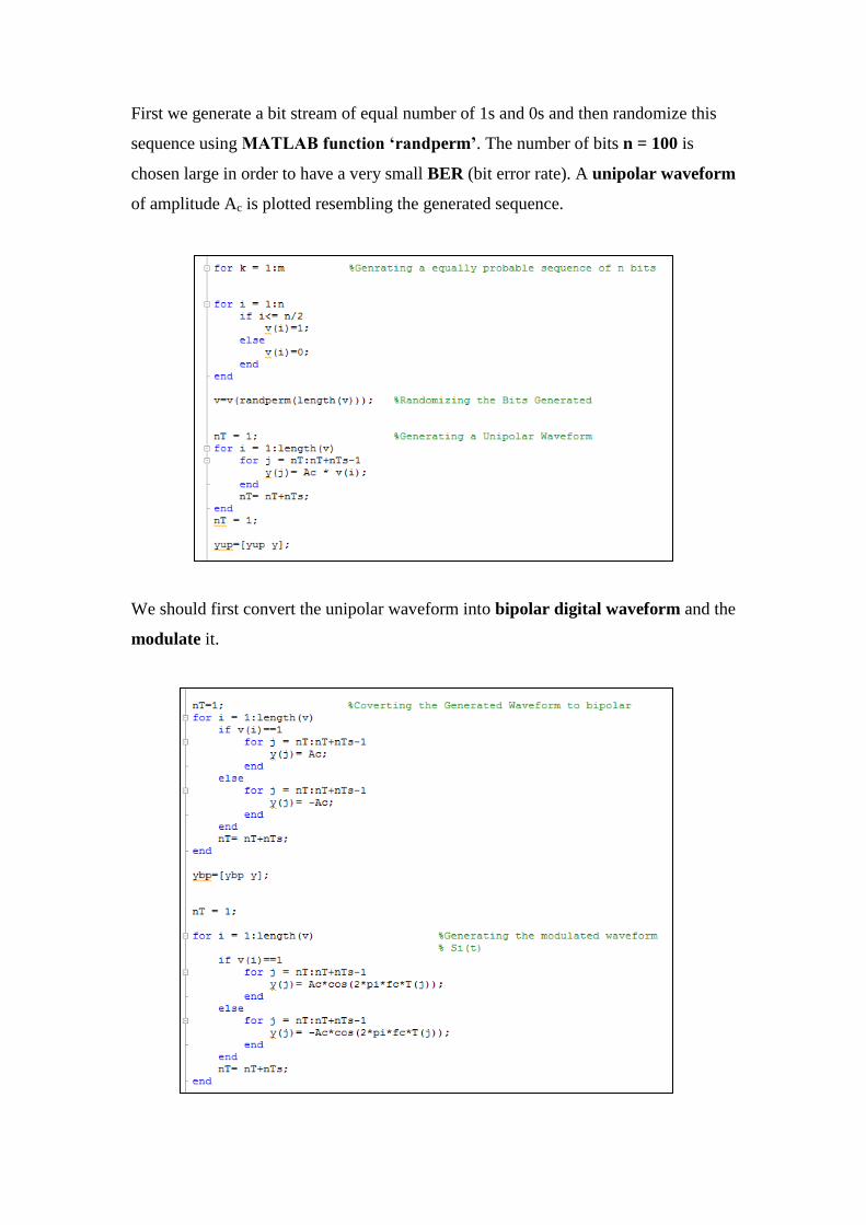
It can now be safely sampled by the receiver at the correct sampling instants,
and compared to an appropriate threshold, resulting in a correct interpretation
of the binary message.
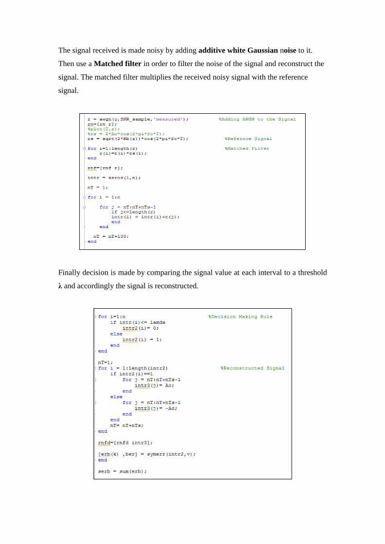
SIMULATION PROGRAMING
In our project we took Ac =1V, and the bit rate Rb=100 Kbits/s. the period Tb should
be a multiple of Tc (fc = k * Rb). In our project we took k=2. The noise for the
AWGN has a power spectral density N0/2= -10-3
W/Hz.The reference signal of the
matched filter rf= √(2/Tb) *cos(2πfct).
a1 is computed by integrating the signal s1* rf over the pit period tb; a2 is computed
similarly with signal s1. Accordingly the threshold λ is calculated by λ=(a1+a2)/2; thus
the threshold is equal to zero since a1 is equal to -a2.
The number of bits n is equal to 500 and the number of loops m is 100 times. In
addition the signal to noise ratio is computed with the given formulas.
First we generate a bit stream of equal number of 1s and 0s and then randomize this
sequence using MATLAB function ‘randperm’. The number of bits n = 100 is
chosen large in order to have a very small BER (bit error rate). A unipolar waveform
of amplitude Ac is plotted resembling the generated sequence.
We should first convert the unipolar waveform into bipolar digital waveform and the
modulate it.
The signal received is made noisy by adding additive white Gaussian noise to it.
Then use a Matched filter in order to filter the noise of the signal and reconstruct the
signal. The matched filter multiplies the received noisy signal with the reference
signal.
Finally decision is made by comparing the signal value at each interval to a threshold
λ and accordingly the signal is reconstructed.

The signal to noise ratio per sample and the probability of error is calculated. A
comparison between the theoretical and the experimental BER is made. The value of
n should be chosen so that the ration should be small typically 1 %. The BER is
plotted against the signal to noise ration Eb/n0 and N the number of bits.
RESULTS
At the Transmitter
Generated Unipolar Signal
Unipolar Signal converted to Bipolar Signal
Figure 1 - Unipolar Signal
Figure 2 - Bipolar Signal
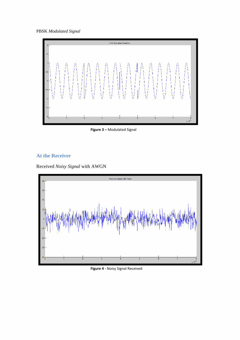
PBSK Modulated Signal
At the Receiver
Received Noisy Signal with AWGN
Figure 4 - Noisy Signal Received
Figure 3 – Modulated Signal
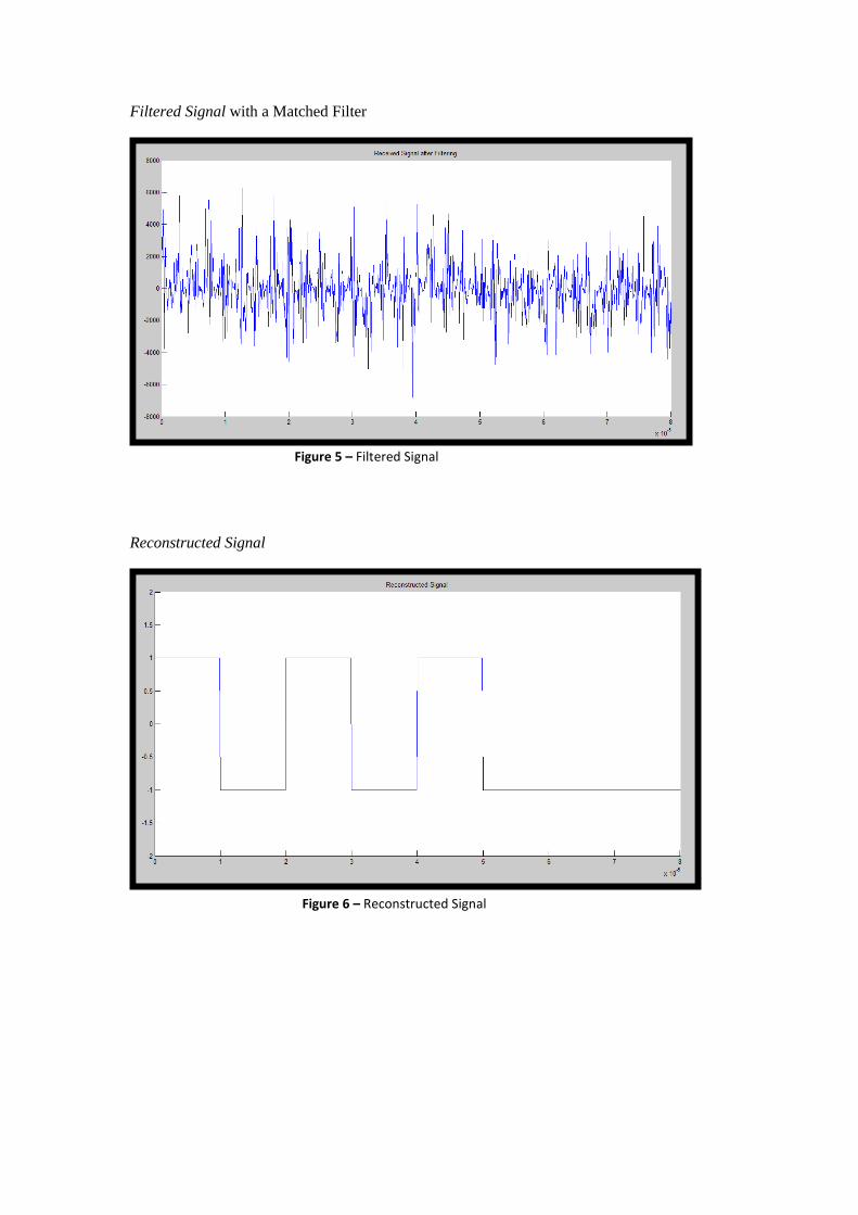
Filtered Signal with a Matched Filter
Reconstructed Signal
Figure 6 – Reconstructed Signal
Figure 5 – Filtered Signal
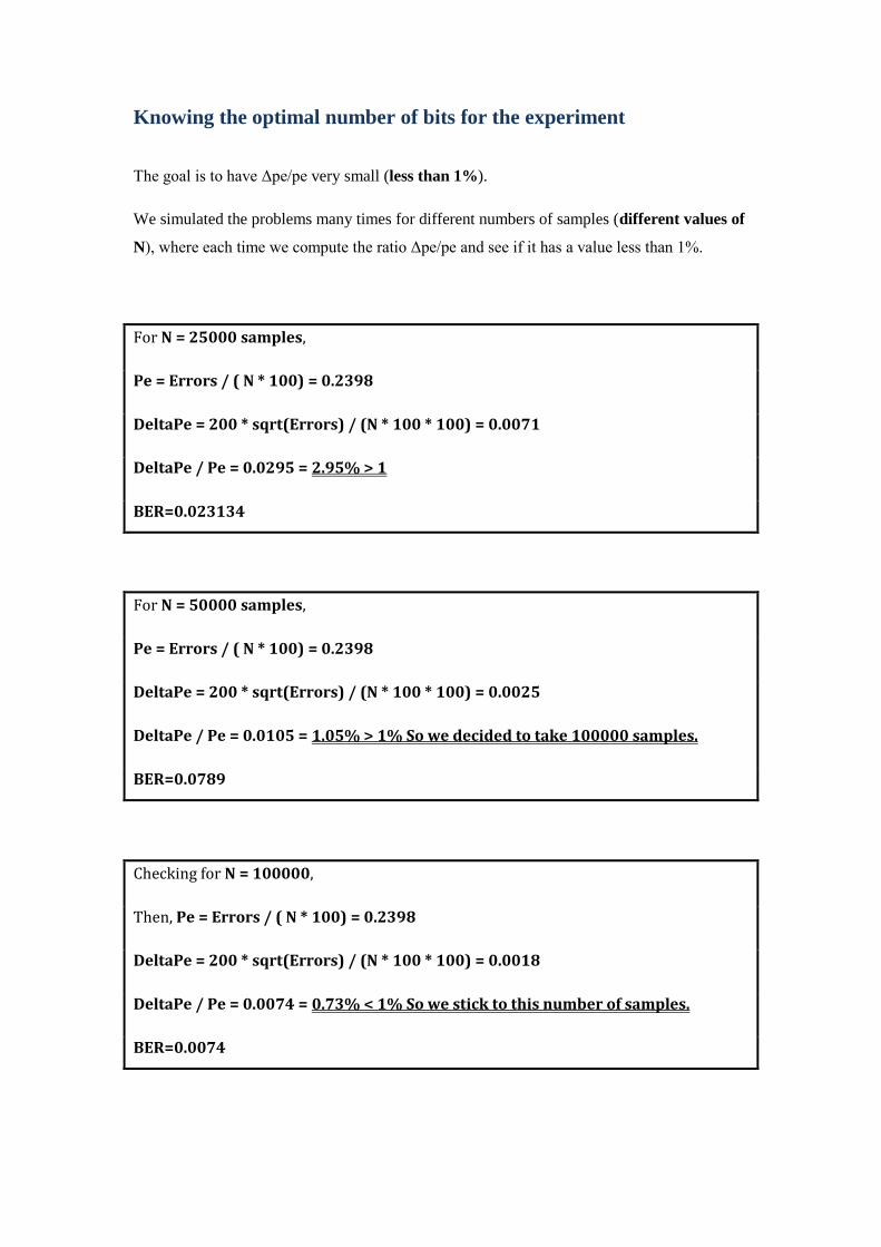
Knowing the optimal number of bits for the experiment
The goal is to have Δpe/pe very small (less than 1%).
We simulated the problems many times for different numbers of samples (different values of
N), where each time we compute the ratio Δpe/pe and see if it has a value less than 1%.
For N = 25000 samples,
Pe = Errors / ( N * 100) = 0.2398
DeltaPe = 200 * sqrt(Errors) / (N * 100 * 100) = 0.0071
DeltaPe / Pe = 0.0295 = 2.95% > 1
BER=0.023134
For N = 50000 samples,
Pe = Errors / ( N * 100) = 0.2398
DeltaPe = 200 * sqrt(Errors) / (N * 100 * 100) = 0.0025
DeltaPe / Pe = 0.0105 = 1.05% > 1% So we decided to take 100000 samples.
BER=0.0789
Checking for N = 100000,
Then, Pe = Errors / ( N * 100) = 0.2398
DeltaPe = 200 * sqrt(Errors) / (N * 100 * 100) = 0.0018
DeltaPe / Pe = 0.0074 = 0.73% < 1% So we stick to this number of samples.
BER=0.0074
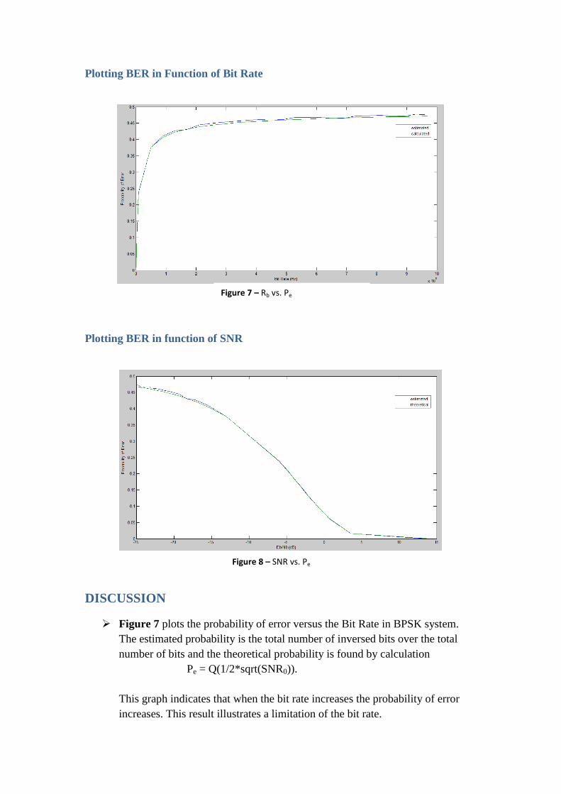
Plotting BER in Function of Bit Rate
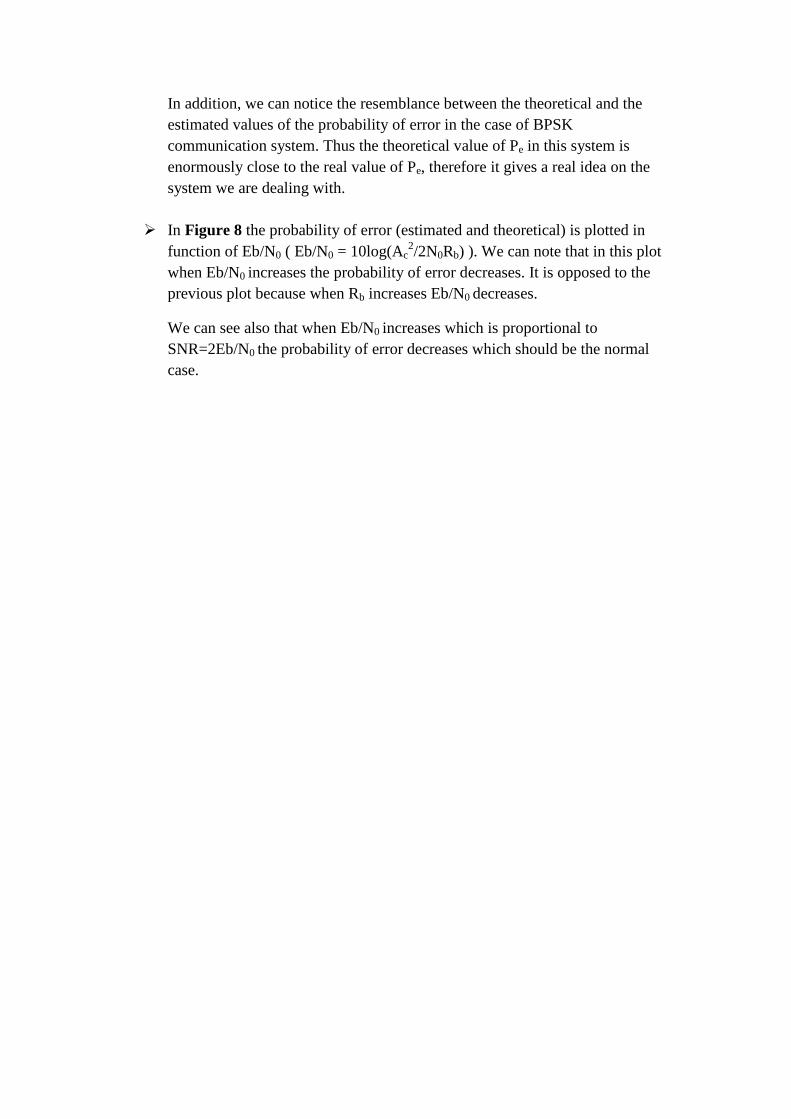
Plotting BER in function of SNR
DISCUSSION
Figure 7 plots the probability of error versus the Bit Rate in BPSK system.
The estimated probability is the total number of inversed bits over the total
number of bits and the theoretical probability is found by calculation
Pe = Q(1/2*sqrt(SNR0)).
This graph indicates that when the bit rate increases the probability of error
increases. This result illustrates a limitation of the bit rate.
Figure 7 – Rb vs. Pe
Figure 8 – SNR vs. Pe
In addition, we can notice the resemblance between the theoretical and the
estimated values of the probability of error in the case of BPSK
communication system. Thus the theoretical value of Pe in this system is
enormously close to the real value of Pe, therefore it gives a real idea on the
system we are dealing with.
In Figure 8 the probability of error (estimated and theoretical) is plotted in
function of Eb/N0 ( Eb/N0 = 10log(Ac2/2N0Rb) ). We can note that in this plot
when Eb/N0 increases the probability of error decreases. It is opposed to the
previous plot because when Rb increases Eb/N0 decreases.
We can see also that when Eb/N0 increases which is proportional to
SNR=2Eb/N0 the probability of error decreases which should be the normal
case.
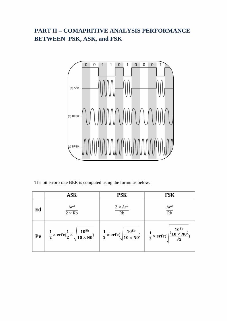
PART II – COMAPRITIVE ANALYSIS PERFORMANCE
BETWEEN PSK, ASK, and FSK
The bit erroro rate BER is computed using the formulas below.
ASK PSK FSK
Ed
Pe
√
√
√
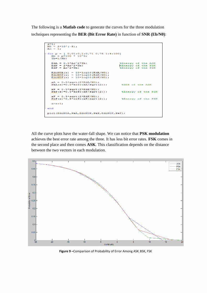
The following is a Matlab code to generate the curves for the three modulation
techniques representing the BER (Bit Error Rate) in function of SNR (Eb/N0):
All the curve plots have the water-fall shape. We can notice that PSK modulation
achieves the best error rate among the three. It has less bit error rates. FSK comes in
the second place and then comes ASK. This classification depends on the distance
between the two vectors in each modulation.
Figure 9 –Comparison of Probability of Error Among ASK, BSK, FSK
DISCUSSION AND CONCLUSION
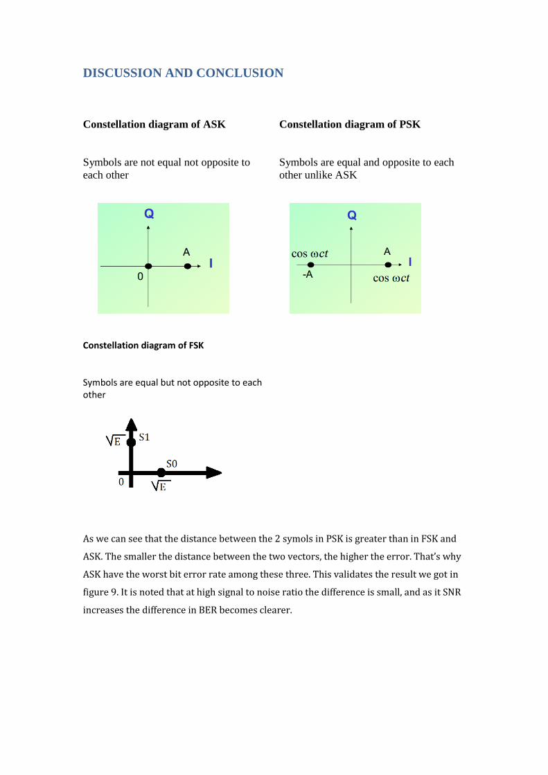
Constellation diagram of ASK
Symbols are not equal not opposite to
each other
Constellation diagram of PSK
Symbols are equal and opposite to each
other unlike ASK
Constellation diagram of FSK Symbols are equal but not opposite to each other
As we can see that the distance between the 2 symols in PSK is greater than in FSK and
ASK. The smaller the distance between the two vectors, the higher the error. That’s why
ASK have the worst bit error rate among these three. This validates the result we got in
figure 9. It is noted that at high signal to noise ratio the difference is small, and as it SNR
increases the difference in BER becomes clearer.