Is Agricultural Zoning Exclusionary?
Paul D. Gottlieb *
Department of Agricultural, Food, and Resource Economics, Rutgers University
Thomas Rudel, Karen O’Neill, and Melanie McDermott
Department of Human Ecology, Rutgers University
* contact at
55 Dudley Road, New Brunswick, NJ, 08901
(732) 932‐9155 x223
Selected Paper prepared for presentation at the Agricultural & Applied Economics Association
2011 AAEA & NAREA Joint Annual Meeting, Pittsburgh, Pennsylvania, July24‐26, 2011
Copyright 2011 by Gottlieb, Rudel, O’Neill, and McDermott.
All rights reserved. Readers may make verbatim copies of this document for non‐commercial
purposes by any means, provided that this copyright notice appears on all such copies.
2
Abstract
In rapidly suburbanizing areas, minimum lot sizes of ten acres or greater are often used to
discourage residential development and to maintain agricultural critical mass. Because of
significant development pressure in these places, there is a good chance these lot size
regulations will bind. Such “down‐zoning” often appears alongside the purchase of agricultural
and conservation easements that reduce housing development even more.
Whatever the benefits of such policies for agriculture and the environment, they raise obvious
concerns about housing supply and affordability. The issue of affordability should be analyzed
at the regional scale, since we would normally expect some high‐income, low density enclaves
to exist within any metropolitan area. In addition, the analyst should look beyond median
home price to compare the distribution of a region’s available housing stock to the distribution
of its income. A primary hypothesized effect of large‐lot zoning is that it skews the distribution
of available housing upward relative to the distribution of income.
The present study will use a unique dataset on the New Jersey Highlands region to help answer
the fundamental question posed by its title. This dataset includes historical data on the lot size
minima imposed on every residential acre in the 83 Highlands municipalities, as well as real
estate listing data on thousands of residential transactions in these 83 municipalities. Data
from the U.S. Census are used to examine the distribution of income among New Jersey
residents who ought to be served by the housing stock in the Highlands.
The study finds that in the 1990s and 2000s, the stock of Highlands housing was skewed high
relative to the metropolitan incomes available to purchase it, even with renters excluded from
the analysis. Using a simple threshold of three times household income, the bottom 30% of
households were consistently able to afford fewer than 30% of the homes coming on the
market, while the top earners could afford a disproportionately large share of the available
housing. At the same time, the study was unable to document a deterioration in Highlands
housing affordability in the 1990s and 2000s that was attributable to anything other than the
national housing bubble. Down‐zoning is likely to affect the mix of housing types on the
margin, while the majority of real estate transactions involve homes that were built several
decades ago. This suggests either a separate analysis of new construction, or a longer time
series on home types and prices that would capture the effects of restrictive zoning over
several decades.
3
Introduction
This paper presents new data on whether agricultural zoning is exclusionary. This claim is often
made by the opponents of such zoning, including farmers’ trade associations. It is also made
by low‐income housing advocates who seek greater access to rural areas for low‐income
populations.
We begin by defining the relevant terms. “Agricultural zoning” will be defined as large
minimum lot sizes (e.g., four to twenty acres) on land that is undeveloped and is suitable for
either agriculture or residential development. In our study area within New Jersey, zones
labeled agricultural generally allow homebuilding by right. The only thing that makes these
zones agricultural is that they are currently farmed and existing lot‐size regulations greatly
reduce their development potential. Either the land in these zones continues in agriculture, or
it is subdivided into five‐acre estates (or larger) that few New Jerseyans can afford. No other
uses are permitted according to the zoning ordinance.1
“Exclusionary zoning” is the term normally applied to zoning that effectively excludes
homebuyers below a certain income level: for example, below the average income of
incumbent residents. The term is also used to denote attempts to exclude minorities from a
particular town (Pendall 2000). Given the lower average income of minorities in the U.S., the
first of these effects virtually guarantees the second, so that the true motive behind
exclusionary zoning can be difficult to discern (Ihlanfeldt 2004; Bogart 1993).
1 Some large‐lot zoning ordinances have a lot‐size averaging feature, which encourages homes on lots smaller than ten acres
next to open space that is permanently preserved. When this option is selected, overall density at the subdivision scale must still be one unit per ten acres. In some cases it can be slightly higher as part of an incentive to cluster development rather than build homes at the maximum density in the usual checkerboard pattern. This incentive is known as a “cluster bonus.”
4
Given these definitions, it would seem that a ten‐acre lot size minimum in an area designated
agricultural would automatically qualify as exclusionary. The reality, however, is more
complicated. A community that enforced ten‐acre zoning in its agricultural zone, but
permitted ten units per acre in a large residential zone nearby, could hardly be characterized as
a place that allows only large country estates. To many urban planners, agricultural zoning has
three goals that are fully consistent with residential inclusion. These planners would argue that
agricultural zoning maintains critical mass in farming in the short run, concentrates residential
development elsewhere in the community, and maintains a contiguous stock of land that can
be deployed in the future if necessary. Agricultural zoning is thus viewed as part of a process of
orderly development, not permanent preservation. The expectation is that large‐lot zoning in
agricultural zones will be relaxed as soon as population pressure becomes great enough to
justify doing so.
What we need, then, is a definition of exclusionary zoning that is more forgiving in terms of
time and space. For purposes of the present paper, exclusionary zoning will be said to exist if it
leads to a distribution of housing stock within the metropolitan area (or a sufficiently large
portion of the metropolitan area) that is skewed high relative to the income distribution of
potential homebuyers. This more regional definition of exclusion also helps to address the
argument – common among academics if not practitioners – that exclusionary zoning by
individual communities is benign, even efficiency‐enhancing, provided that a large selection of
communities and housing types exists at the level of the metropolitan area (Hamilton 1976;
Fischel 2005).
This definition of exclusionary zoning will be explored using a unique cross‐section time series
dataset on agricultural/residential zoning in the New Jersey Highlands, an area encompassing
83 municipalities that became the subject of a new regional planning initiative in 2004 (see
Gottlieb, 2005). We argue that this region is so large, it really ought to accommodate the full
diversity of incomes in northern New Jersey. Over the last thirty years, however, minimum lot
sizes on agricultural land in the Highlands have been increasing, while a significant amount of
open space has been permanently barred from development (Rudel, et al., 2011). Our
5
hypothesis is that these policy choices increased the average price of housing in the Highlands
and contributed to an increase in the proportion of housing units at the upper end of the price
distribution. These trends, in turn, should cause a comprehensive measure of housing
affordability to deteriorate.
A literature review is followed by a description of the data. The results section includes
histograms for zoned acres, residential transaction prices, and the lot sizes of homes that have
been sold in multiple years. The key indicator of affordability is based on home prices as a
multiple of household income. Using an innovative method that is similar to the Lorenz curve
(Gan and Hill 2009), the entire distribution of home prices in each year is compared to the
entire distribution of northern New Jersey incomes. The effect of the national housing bubble
is controlled away by adjusting mean income upward over time so that it tracks the time trend
in the quality‐controlled price of housing in the New York metropolitan area. This allows us to
isolate the main hypothesized effect of restrictive zoning, which is to skew the distribution of
available housing upward. Without this adjustment, the effects of zoning and of the housing
bubble are effectively combined. Those results are also reported.
Past literature on exclusionary zoning
The last decade’s housing bubble generated new concerns about housing affordability, along
with many works seeking to explain both the causes of the bubble and the differences in its
intensity across metropolitan areas. Among the more influential works in the latter category
have been those by Glaeser and Gyourko (Glaeser and Gyourko 2003; Glaeser, Gyourko, and
Saks 2005). These authors argue that what needs to be explained is not the gap between U.S.
home prices and incomes, but rather the gap between home prices and construction costs.
This is because construction costs provide us with a market standard of a fair price that can be
used as a starting point for affordability analysis. Glaeser and Gyourko are especially
concerned that metropolitan areas with very large gaps between home prices and construction
costs use zoning and other regulations to restrict new housing supply. Their theoretical
arguments and empirical results provide support for this view, as against alternative
6
explanations like especially strong business demand or a shortage of developable land. Thus
Glaeser and Gyourko have given new life to the old critique of suburban zoning as exclusionary,
a theme that has also been taken up by a handful of academic planners (Levine, 2006).
The idea that large‐lot zoning and related regulatory restrictions increase home prices is, of
course, not new. In a review of the relevant literature, Keith Ihlanfeldt (2004) concludes that
the empirical evidence for this proposition is strong, and includes both supply‐ and demand‐
side effects (e.g., large‐lot zoning creates higher amenity neighborhoods that fetch higher
prices per square foot). Two empirical articles within the group reviewed by Ihlanfeldt are
worth mentioning because they focus on the poor (Zorn, Hansen, and Schwartz, 1986) and on
minorities (Pendall 2000). Pendall’s work yielded especially strong results for density
restrictions, as opposed to other types of local land use control. Other review articles agree
with Ihlanfeldt that zoning restrictions are correlated with higher home prices, but they are
more circumspect about the literature’s overall reliability (Pogodzinski and Sass 1991; Quigley
and Rosenthal 2005). The primary caution in these latter articles is that the direction of
causation between zoning and home prices ‐‐ or between zoning and obvious correlates of
home prices, like income ‐‐ remains unclear.
The present study will not attempt to prove a causal link between changes in zoning and
changes in residential transaction prices in the Highlands region. Instead, it will demonstrate a
mild correlation between these two concepts over time. It must be remembered that the
increase in minimum lot sizes observed in the region over the last thirty years affects a
relatively small proportion of the homes brought to market in a given year, mostly new
construction. That being said, residential transaction prices increased continuously in the
Highlands region between 1996 and 2004, while the rightward skewness of prices increased up
until the recession of the early 2000s. We know that the decade after 1995 witnessed a
significant degree of down‐zoning statewide (Adelaja and Gottlieb 2009), coinciding with the
effects of the national housing bubble. What remains to be seen is if housing in the region
became less affordable over this period, using a measure that captures the full distribution of
home prices and of the incomes of potential buyers.
7
The inferential approach taken here is similar to that used in a companion piece analyzing the
same region (Rudel, et al. 2011). That piece also noted the increase in minimum lot sizes in the
Highlands and the significant amount of open space set‐asides occurring there in recent years.
But its measure of exclusion was even more direct: It reported evidence of a redistribution of
population growth from the Highlands region to the inner suburbs of New Jersey in the 1990s.
Because metropolitan development normally moves outward, this was seen as evidence that
communities in the Highlands had effectively “pulled up the drawbridge” over this period
(Rudel, et al. 2011). The title of this earlier article, “from middle to upper‐class sprawl?”,
captures the hypothesized changeover to larger residential lots enforced by increasing lot size
restrictions.
The present paper uses Rudel et al’s data on minimum lot‐size zoning to make an argument not
about supply, but about the related issue of affordability. This requires, of course, some data
on home prices. The articles by economists cited above have paid a great deal of attention to
prices; the problem is that they tend to ignore the most obvious exclusionary effect of region‐
wide zoning restrictions. This is zoning’s effect on the mix of homes brought to market, rather
than on the price of a quality‐adjusted home. Hedonic analysis, which makes up the majority
of economic research on the price effects of zoning, intentionally controls away the attributes
of homes that make them more expensive, such as lot size and the number of rooms. Similarly,
by focusing only on the gap between market prices and construction costs, Glaeser and
Gyourko ignore the regional distribution of dwelling construction costs (i.e., types of homes)
that zoning may encourage or discourage in a given housing market. The distribution of
available housing products matters a great deal, of course, to lower‐income residents. Thus the
present study explores exclusionary zoning in a common‐sense way that is largely missing from
the existing literatures in agricultural and urban economics.
Data and approach
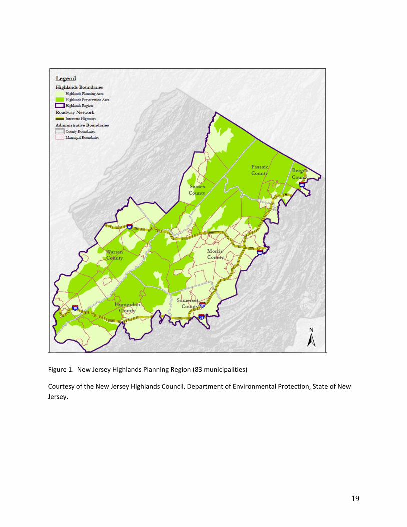
The study region consists of 83 municipalities in the New Jersey Highlands, an exurban area in
the northwestern part of the state (Figure 1). The southern half of this region tends toward

8
agricultural use, while the northern half is mountainous with significant forest cover. A
significant amount of land use and regulatory data are available on these 83 communities. This
is because they were placed under the authority of a new regional planning board in 2005, on
the basis of federal research that highlighted the importance of this region to the state’s water
supply (Gottlieb, 2005; Phelps and Hoppe, 2002).
For purposes of the present study, two things should be noted about the study region. First, it
is large enough that one can argue it ought to provide the full range of housing to serve all
income groups in New Jersey (see the map in Figure 1). It should be noted that under New
Jersey’s Mount Laurel court decisions, each municipality is theoretically obligated to provide its
own “fair share” of affordable housing. Extending this obligation to a multi‐county region is
presumably justified. Second, the zoning and homebuilding decisions in this region occurred
largely before the Highlands Planning Act was passed in 2004—and certainly before binding
state regulations were promulgated. For the most part, then, they reflect private market
decisions constrained by local rather than state regulations. In the conclusion we return to the
question of whether our empirical findings are tainted by these two types of state‐level control:
Statewide affordable housing regulations that were on the books before the study period
began, and a regional planning regime that began just after the study period ended.
GIS data on minimum lot size zoning for 1995 were collected by Rutgers University’s Grant
Walton Center for Remote Sensing and Spatial Analysis, as part of the body of work that helped
inform the Highlands Planning Act of 2004. This dataset was then extended back and forward
in time under the terms of a Human Systems Dynamics grant from the National Science
Foundation. This data collection effort provided minimum lot sizes in each residential zone
shown on municipal zoning maps for various years, as well as a complete inventory of acres
permanently preserved by municipalities, by the state, and to a lesser degree by private
conservation organizations (see Rudel, et al., 2011).
Data on home prices and characteristics were collected from the web site of the Garden State
Multiple Listing Service (MLS), which is the primary sales support and tracking tool used by
licensed real estate brokers. All of the MLS data used in this study are actual closing prices;
9
ordinary homebuyers using the website see only offer prices. The data contained in the MLS
database are rich, including closing date, closing price, location, and just about all of the home
characteristics one would expect to see on a broker’s spec sheet. There are two drawbacks,
however. Computer‐readable data go back only to the mid‐1990s, and they need a lot of
cleaning because they are entered by brokerage staff who have no need to standardize input
with a view to creating analyzable datasets. In particular, data on the lot sizes of sold homes
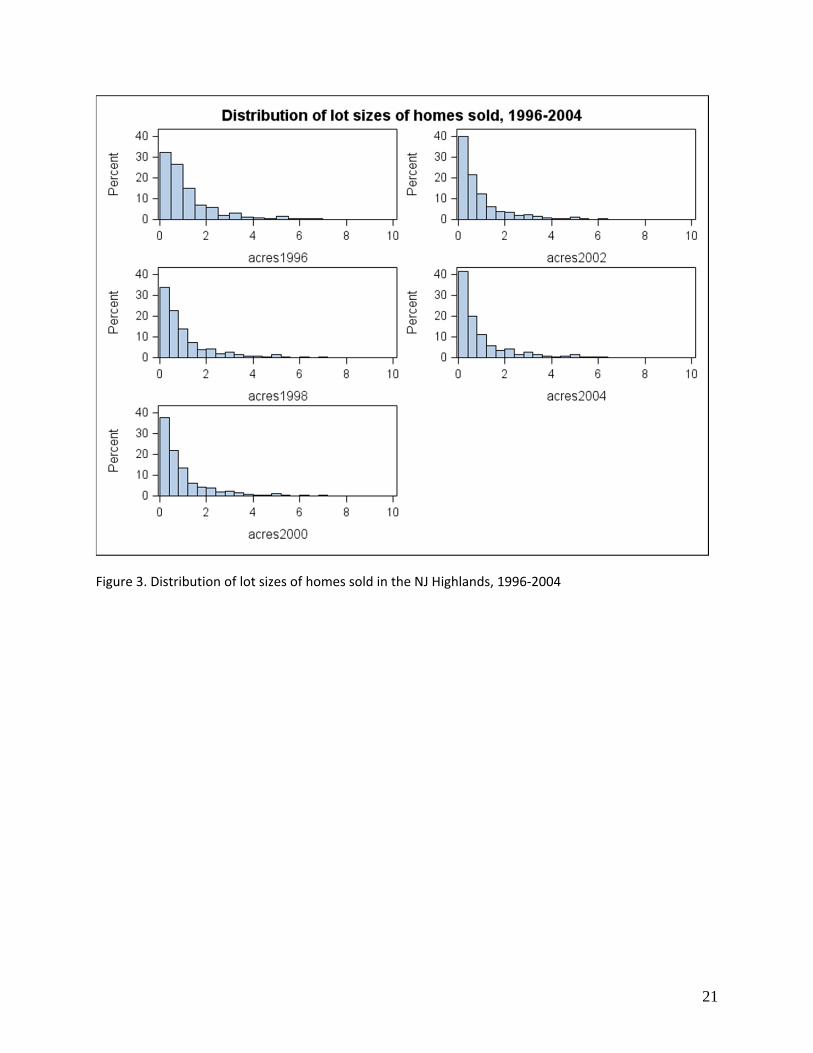
are available for only 41% of the observations in the Highlands MLS dataset (these data are
described in Figure 3 and Table 2).
These three variables ‐‐ minimum lot sizes, lot sizes of sold homes, and closing prices ‐‐ are
explored in the Highlands region using histograms and simple univariate statistics. The goal is
to see how the moments of the distributions change over time. In order to determine if the
distribution of housing in the Highlands has been getting more or less affordable for a given
reference population, it is necessary to define that population and then measure the
distribution of its household income. For simplicity, we assume that the mix of housing in the
Highlands should be affordable to the range of incomes that existed in northern New Jersey in
the year 1990. Northern New Jersey is defined as the following twelve counties: Bergen, Essex,
Hudson, Hunterdon, Mercer, Middlesex, Morris, Passaic, Somerset, Sussex, Union, and Warren.
The distribution of household income is available in the 1990 census for each of these counties,
and is easily aggregated. We collected the income distribution for owner‐occupiers only. This
is because we only have 1995‐2004 multiple listing service data for single‐family detached
homes. To include renters among the potential buyers of such homes without including multi‐
family units on the supply side appears misleading. This choice of reference population,
however, parallels arguments made in our earlier work entitled “from middle to upper class
sprawl.”
One goal of this study is to look for inequities in the distribution of the housing stock at a single
point in time, such as 1995 or 2000. A second goal is to see if a measure of affordability
changes with changes in the housing stock, holding the distribution of income constant. We
intentionally measure the household income distribution in the start year only, because we

10
want to ensure that it is exogenous to subsequent changes in the mix of housing supply. This
does not mean that our measure of 1990 income remains fixed in nominal terms: It shouldn’t.
Two different methods are used to inflate the bracket endpoints from the 1990 income
distribution data to years for which we have a good number of home price observations: 1995,
2000, and 2004. For the first affordability analysis, we inflate 1990 income using the federal
Consumer Price Index for the New York metropolitan area. This is a standard method of
estimating actual income in a year for which there is no census survey. For the second
affordability analysis, we inflate 1990 income using the Case‐Schiller quality‐adjusted home
price index for the New York metropolitan area, which is available on the website of Standard
and Poor’s. We do this in an effort to control away the effects of the 2000s housing bubble. If
1990 incomes are increased by exactly enough to cover the New York “bubble premium,” than
any remaining gap in affordability must be the result of a change in the housing stock.
An innovative housing affordability graphic is used to compare the distribution of incomes to
the distribution of home prices. As described in Gan and Hill (2009), this technique allows one
to look at both distributions together, while standard approaches, such as those that track
median home prices, ignore much of the distributional information available on both the
demand and supply sides. And yet the technique is not difficult to understand, especially if
you are familiar with the Lorenz curve that is commonly used to summarize a country’s income
distribution with a single comprehensive graph and parameter.
In this technique, all households are lined up in rank order on the horizontal axis, with the
richest ones on the left and the poorest on the right. We then calculate and graph a set of
coordinate pairs according to the following example: The richest 10% of the population can
afford, say, 86% of the homes on the market given the distribution of incomes and home prices
we have collected. The definition of “afford” is the realtor’s simple rule‐of‐thumb: In the case
of the present study, a home is regarded as affordable if its price is no more than three times a
household’s income.
11
The reason why the richest 10% can afford only 86% of the homes on the market (or 93% or
90% or 82%) is that the poorest member of the top 10% sets the limit. Every member of the
top 10% must be able to afford every home in the cumulative percentage of homes for this
group. The poorest member of the top tenth might have an income that is only one‐third of
the number sitting at the 86th percentile of home prices. If that is true, then everybody in the
top 10% will be able to afford 86% of the homes‐‐‐but nothing more. By the same logic, the
top 100% of incomes can afford 0% of the homes, because the income on the very bottom will
typically be unable to afford anything (using the multiple of three times income). Note that the
45‐degree line describes an equitable affordability profile, with the percentage of homes
affordable to each group exactly proportional to the group’s distribution in the population.
See figures 5 and 6.
Results
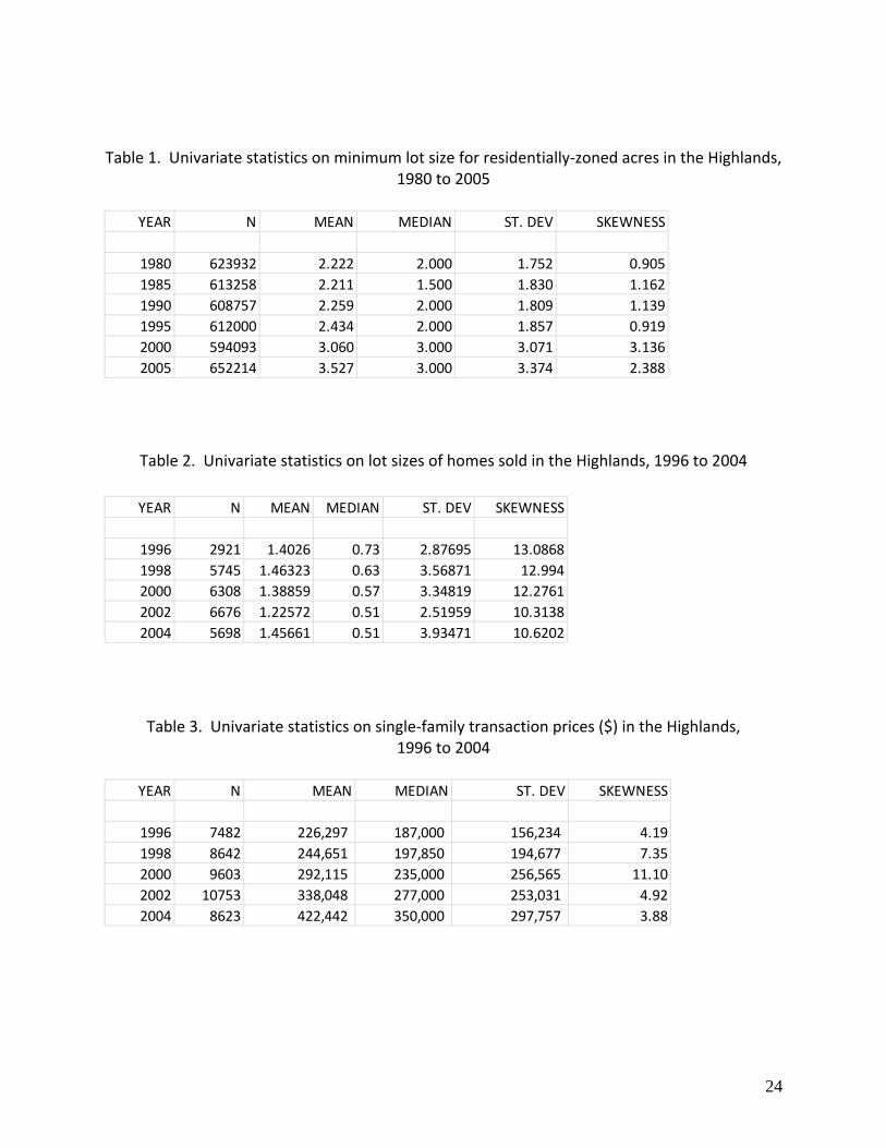
The data show a consistent increase in the average minimum lot size of residentially‐zoned
acres after the year 1990 (Table 1). Minimum lot sizes are not normally distributed, but they
spike at several common numbers, like half an acre or five acres. Figure 2 shows that the
percentage of residential acres zoned for a minimum of five acres rose from below 20% in 1985
to more than 30% twenty years later. This is the most popular lot size minimum for
agricultural and forested acres in the Highlands. Four‐acre minimum lot size zoning has also
increased from less than 1% of the total to close to 8%. Meanwhile, the smallest lot size
categories have fallen to less than 20% of total acres. There were also increases in the
prevalence of both 10‐ and 20‐acre minima, but the latter are a small minority of total acres
and are omitted for readability.
Table 2, based on the 41% of homes in the real estate dataset that have lot size data, does not
show a consistent increase in the lot sizes of the homes actually sold in each year. Instead
these data look cyclical, with smaller‐lot homes sold during the 2001‐2002 recession than
during the boom periods of the late 1990s and mid‐2000s. These data remind us that real
estate transaction data reflect not only the underlying stock of housing potentially available for
12
purchase, but also changes in demand that might be driven by purchasing power. The
cyclicality in the data also suggests the need for a longer time series, currently unavailable from
the MLS, that would capture structural changes on both the demand side and the supply side.
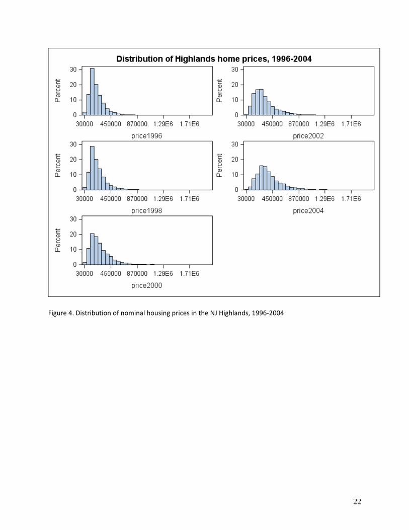
Table 3 and Figure 4 measure the distribution of nominal home prices for selected years
between 1996 and 2004. The steady increase in mean home prices reflects both regulatory
restrictions (possibly) and the national housing bubble; there is a marked acceleration in home
prices in the early 2000s. Of greater interest, perhaps, is the statistic on rightward skewness,
which increased through 2000 before falling back down. This trend may be related to the up
and down trend in the lot sizes of homes sold shown in Table 2.
Figures 5 and 6 compare the distribution of home prices in multiple years to the distribution of
household income (excluding renters) in the twelve counties surrounding the Highlands in
1990. In Figure 5, the New York metro CPI is used to inflate the breakpoints of the 1990
income distribution to match the years for which home price data are available. In Figure 6,
the Case‐Schiller index for the New York metro is used for the same purpose. Thus Figure 6
corrects more completely for the housing bubble, since it uses a price index for a market basket
that contains quality‐adjusted housing only.
Before discussing the time trend, we observe that the distribution of home prices is generally
inequitable using the 45‐degree line criterion based on the 3 x income standard. Unlike the
Lorenz curve for income distribution, observations in Figures 5 and 6 can lie above or below the
45‐degree line. Equity problems might be indicated when points at the upper end of the
income distribution lie “Northeast” of a 45‐degree line and points at the lower end of the
income distribution lie “Southwest” of a 45‐degree line. This backwards S‐shape of the
affordability profile is evident in all scenarios except those where affordability is poor for
everybody, such as year 2004 in Figure 5.
While zoning regulations could have contributed to the relative lack of Highlands homes priced
at less than three times the lowest incomes, Figures 5 and 6 would be more persuasive if they
were compared to the same graph from an unregulated region. Even in the absence of supply
restrictions, it is rarely the case that people choose to spend exactly the same proportion of

13
their incomes on a good like housing, no matter how much they earn. The standard
affordability threshold of three times income should presumably be adjusted to account for the
possibility that the income elasticity of demand for housing is less than 1.0.2
If a backwards S‐curve in the data is to be expected, then zoning restrictions might cause
affordability problems that increase for northern New Jerseyans over time, since we know that
the average minimum lot size has been increasing. So the goal now is to see if all or most of
the points in Figures 5 and 6 move northeast or southwest over time.
In both figures, the changes in affordability over time are systematic but run in opposite
directions. Figure 5 shows the change in affordability using our best estimate of what incomes
actually were in 1995, 2000, and 2004. Housing became less affordable for all quantiles in this
period, increasing markedly between 2000 and 2004. The most likely explanation for this result
is the across‐the‐board increase in transaction prices caused by the housing bubble. A simple
way to remove the effects of the bubble is to inflate the incomes of potential buyers using the
best available index of bubble prices. This is done in Figure 6, and the points now move to the
northeast over time, with the possible exception of the very poorest quantiles. We are
therefore unable to measure any decline in housing affordability in the Highlands that was
driven by any cause other than the national housing bubble. Indeed, controlling for the housing
bubble, there actually appears to be a slight increase in affordability over this period when
home prices are measured using transaction price data.
Conclusion
This study uses a straightforward – we would argue correct – method to measure the
exclusionary impact of lot size restrictions in a single metropolitan area. That is because such
zoning has three exclusionary effects, in theory: (1) It lowers the overall stock of housing that is
allowed in the long run; (2) It raises the price‐per‐square‐foot of homes in the short run by
2 The income elasticity of demand for housing has been estimated in the range of .6 to .7 using permanent income (Carliner,
1973). For more recent estimates using US data, see Hansen, Formby, and Smith (1998).
14
increasing amenities and making the homes harder to build; (3) It skews the distribution of
available homes in an upscale direction, even if the incomes of those who might buy the homes
are not similarly skewed.
Theoretical reason #1 is an arithmetic fact, but its impact on prices in the short run is unclear.
Theoretical reason #2 is where the bulk of work by economists has taken place. It seems to us
that this pathway ignores the dominant exclusionary effect, which is that homes are simply
bigger and more expensive in those metropolitan areas where small homes are prohibited on a
significant percentage of the developable acres.
The fact that we have selected the most logical pathway for zoning to be exclusionary does not
mean that it is the easiest one to measure or to prove. Because the geographic unit of analysis
is an entire housing market, we effectively have only one observation in this study. Minimum
lot sizes and home prices (as well as other relevant factors) have increased over time, giving us
what is effectively a time series problem on this single geographic observation. Moreover, the
covariates in such a time series analysis would consist of the moments of various distributions,
the argument being that one distribution (lot size minima) must eventually influence others
(delivered lot sizes and associated prices), all in a world where much of the housing stock is a
legacy handed down to us from before the study period began. Indeed, one insight from the
analysis is that changes in zoning affect the distribution of housing transactions through their
effects on new construction, so it may take decades for such effects to be observed. Yet MLS
price data are not available before 1994.
One obvious criticism of our housing price data is that they do not measure supply as shaped by
zoning, but rather by the intersection of supply and demand. The first question to be asked is
if some kinds of homes change hands more frequently than other kinds of homes. If so, then a
database of transaction prices will not reflect the true underlying distribution of the stock of
housing. The frequency with which certain types of homes change hands can also change over
time in response to cyclical or demographic demand considerations, as we suggested in our
discussion of Table 2. The solution to this problem is to use home price data from census
questionnaires or tax assessment records. The census approach also permits a longer time‐
15
span of home price data to be collected in a consistent way; the downside is that prices are self‐
reported. We are currently pursuing this line of additional research.
The study area chosen for this analysis presents two additional challenges. First, each of the 83
Highlands municipalities is required to supply a certain amount of affordable housing under the
regulatory framework of New Jersey’s Council on Affordable Housing. In our opinion this has
not affected the present paper’s results for two reasons: (1) The provision of Mount Laurel
housing throughout the state is well below targets because of chronic litigation and foot‐
dragging; (2) Mount Laurel Housing is mostly multi‐family.
Second, we have examined home prices in a ten‐year period immediately preceding the
enactment of a regional planning law that developers worried would significantly close off land
to development. This could, in fact, be one explanation for the observed fall in the lot sizes
delivered in 2002, as developers scrambled to build as much as they could before the Highlands
planning law went into effect.
The regional planning law moved through the legislature very rapidly, however, and developers
would have to have been excellent political forecasters to put such projects into their pipelines
in 1999 or 2000. And because most transactions involve homes that are not even new, the
recession seems a more convincing explanation of the trend in Table 2.
The solution to this problem, as with so many of the others, is to collect home price data in the
Highlands for the same period as the available zoning data, roughly 1975 to 2005.
References
Adelaja, A.O., and P.D. Gottlieb. 2009. The political economy of downzoning. Agricultural and Resource Economics Review 38(2):1‐10.
Bogart, William T. 1993. “‘What Big Teeth You Have!’: Identifying the Motivations for
Exclusionary Zoning.” Urban Studies 30 (10) (December 1): 1669‐1681.
16
Carliner, Geoffrey. 1973. “Income Elasticity of Housing Demand.” The Review of Economics and Statistics 55 (4) (November 1): 528‐532.
Fischel, William. 2005. The Homevoter Hypothesis. Cambridge, MA: Harvard University Press.
Gan, Quan, and Robert Hill. 2009. “Measuring housing affordability: Looking beyond the median.” Journal of Housing Economics 18: 115‐125.
Glaeser, EL, and J. Gyourko. 2003. “The impact of zoning on housing affordability.” Economic Policy Review 9 (2): 21‐39.
Glaeser, E, Joseph Gyourko, and Raven Saks. 2005. “Why have housing prices gone up?” AEA Papers and Proceedings (May).
Gottlieb, P. 2005. Summary of the New Jersey Highlands Water Protection and Planning Act. Online Fact Sheet of Rutgers Cooperative Extension, New Jersey Agricultural Experiment Station. Accessed on 4/27/09 at http://njaes.rutgers.edu/highlands/.
Hamilton, B., 1976. "Capitalization of interjurisdictional differences in local tax prices." American Economic Review 66, 743‐753.
Hansen, Julia L., John P. Formby, and W. James Smith. 1998. “Estimating the Income Elasticity of Demand for Housing: A Comparison of Traditional and Lorenz‐Concentration Curve Methodologies.” Journal of Housing Economics 7 (4) (December): 328‐342.
Ihlanfeldt, Keith R. 2004. “Exclusionary Land‐use Regulations within Suburban Communities: A Review of the Evidence and Policy Prescriptions.” Urban Studies 41 (2) (February): 261‐283.
Levine, Jonathan. 2006. Zoned out: Regulations, markets, and choices in transportation and
metropolitan land‐use. Washington, DC: Resources for the Future.
Pendall, Rolf. 2000. “Local land use regulation and the chain of exclusion.” Journal of the American Planning Association 66 (2): 125‐142.
Phelps, M., Hoppe, M., eds., 2002. New York‐New Jersey Highlands Regional Study: 2002 Update. US Forest Service, United States Department of Agriculture, Report NA‐TP‐02‐03.
Pogodzinski, J.M., and Tim Sass. 1991. “Measuring the effects of municipal zoning regulations: A survey.” Urban Studies 28 (4): 597‐621.
17
Quigley, John, and L.A. Rosenthal. 2005. “The effects of land use regulation on the price of housing: What do we know? What can we learn?” Cityscape 8 (1): 69‐137.
Rudel, Thomas K., Karen O’Neill, Paul D. Gottlieb, Melanie McDermott, and Colleen Hatfield.
2011. “From middle to upper class sprawl? Land use controls and changing Patterns of real
estate development in northern New Jersey.” Annals of the Association of American
Geographers 101 (3): 609.
Zorn, Peter M., David E. Hansen, and Seymour I. Schwartz. 1986. “Mitigating the Price Effects of Growth Control: A Case Study of Davis, California.” Land Economics 62 (1) (February 1): 46‐57.

18
Figures and tables
19
Figure 1. New Jersey Highlands Planning Region (83 municipalities)
Courtesy of the New Jersey Highlands Council, Department of Environmental Protection, State of New
Jersey.
20
1980
1995
1985
2000*
1990
2005*
Figure 2. Distribution of residential acres by minimum lot size in NJ Highlands communities, 1980‐2005
(* a small right‐hand tail is omitted for readability and comparability.)
05
1015
20P
erce
nt
0 2 4 6 8 10mls
05
10
15
20
25
Pe
rce
nt
0 2 4 6 8 10mls
05
1015
2025
Per
cent
0 2 4 6 8 10mls
05
10
15
20
25
Pe
rce
nt
0 2 4 6 8 10mls
05
1015
2025
Per
cent
0 2 4 6 8 10mls
010
2030
Per
cent
0 2 4 6 8 10mls
21
Figure 3. Distribution of lot sizes of homes sold in the NJ Highlands, 1996‐2004
22
Figure 4. Distribution of nominal housing prices in the NJ Highlands, 1996‐2004

23
Figure 5. Housing affordability Lorenz curve with 1990 incomes adjusted using the New York metropolitan area Consumer Price Index.
Figure 6. Housing affordability Lorenz curve with 1990 incomes adjusted using the Case‐Schiller housing price index for the New York metropolitan area.
0%
10%
20%
30%
40%
50%
60%
70%
80%
90%
100%
0% 20% 40% 60% 80% 100%Cumulative % of homes affordab
le
Cumulative % of households
1995 2000 2004
0%
10%
20%
30%
40%
50%
60%
70%
80%
90%
100%
0% 20% 40% 60% 80% 100%Cumulative % of homes affordab
le
Cumulative % of households
1995 2000 2004
24
Table 1. Univariate statistics on minimum lot size for residentially‐zoned acres in the Highlands, 1980 to 2005
Table 2. Univariate statistics on lot sizes of homes sold in the Highlands, 1996 to 2004
Table 3. Univariate statistics on single‐family transaction prices ($) in the Highlands, 1996 to 2004
YEAR N MEAN MEDIAN ST. DEV SKEWNESS
1980 623932 2.222 2.000 1.752 0.905
1985 613258 2.211 1.500 1.830 1.162
1990 608757 2.259 2.000 1.809 1.139
1995 612000 2.434 2.000 1.857 0.919
2000 594093 3.060 3.000 3.071 3.136
2005 652214 3.527 3.000 3.374 2.388
YEAR N MEAN MEDIAN ST. DEV SKEWNESS
1996 2921 1.4026 0.73 2.87695 13.0868
1998 5745 1.46323 0.63 3.56871 12.994
2000 6308 1.38859 0.57 3.34819 12.2761
2002 6676 1.22572 0.51 2.51959 10.3138
2004 5698 1.45661 0.51 3.93471 10.6202
YEAR N MEAN MEDIAN ST. DEV SKEWNESS
1996 7482 226,297 187,000 156,234 4.19
1998 8642 244,651 197,850 194,677 7.35
2000 9603 292,115 235,000 256,565 11.10
2002 10753 338,048 277,000 253,031 4.92
2004 8623 422,442 350,000 297,757 3.88


![THE ECONOMICS OF EXCLUSIONARY ZONING … collapse of the U.S. housing bubble has led to a massive oversupply of housing, ... 2009] Economics of Exclusionary Zoning and Affordable Housing](https://static.cupdf.com/doc/110x72/5ad867f27f8b9a98098e020c/the-economics-of-exclusionary-zoning-collapse-of-the-us-housing-bubble-has.jpg)