Ionospheric electron densities at Mars: Comparison
of Mars Express ionospheric sounding and MAVEN
local measurementsF. Nemec
1, D. D. Morgan
2, C. M. Fowler
3, A. J. Kopf
2, L. Andersson
3, D. A.
Gurnett2, D. J. Andrews
4, V. Truhlık
5
Frantisek Nemec, [email protected]
1Faculty of Mathematics and Physics,
Charles University, Prague, Czech Republic
2Department of Physics and Astronomy,
University of Iowa, Iowa City, Iowa, USA
3Laboratory for Atmospheric and Space
Physics, University of Colorado Boulder,
Boulder, Colorado, USA
4Swedish Institute of Space Physics,
Uppsala, Sweden
5Institute of Atmospheric Physics, The
Czech Academy of Sciences, Prague, Czech
Republic
This article has been accepted for publication and undergone full peer review but has not been throughthe copyediting, typesetting, pagination and proofreading process, which may lead to differencesbetween this version and the Version of Record. Please cite this article as doi: 10.1002/2017JA024629
c⃝2017 American Geophysical Union. All Rights Reserved.

Abstract. We present the first direct comparison of Martian ionospheric
electron densities measured by the Mars Advanced Radar for Subsurface and
Ionospheric Sounding (MARSIS) topside radar sounder on board the Mars
Express spacecraft and by the Langmuir Probe and Waves (LPW) instru-
ment on board the Mars Atmosphere and Volatile Evolution Mission (MAVEN)
spacecraft. As low electron densities are not measured by MARSIS due to
the low power radiated at low sounding frequencies, MARSIS electron den-
sity profiles between the local electron density and the first data point from
the ionospheric sounding (≈ 104 cm−3) rely on an empirical electron den-
sity profile shape. We use the LPW electron density measurements to im-
prove this empirical description, and thereby the MARSIS derived electron
density profiles. We further analyze four coincident events, where the two
instruments were measuring within a five degree solar zenith angle (SZA)
interval within one hour. The differences between the electron densities mea-
sured by the MARSIS and LPW instruments are found to be within a fac-
tor of two in 90% of measurements. Taking into account the measurement
precision and different locations and times of the measurements, these dif-
ferences are within the estimated uncertainties.
c⃝2017 American Geophysical Union. All Rights Reserved.

Keypoints:
• MAVEN LPW electron density measurements used to improve the re-
sults of MARSIS ionospheric sounding
• LPW and MARSIS electron densities compared for four coincident events
• Good agreement between the two data sets, MARSIS electron densities
typically slightly larger
c⃝2017 American Geophysical Union. All Rights Reserved.

1. Introduction
Electron densities in the Martian ionosphere are now routinely measured both by
the Mars Advanced Radar for Subsurface and Ionospheric Sounding (MARSIS) topside
radar sounder on board the Mars Express spacecraft and by the Langmuir Probe and
Waves (LPW) instrument on board the Mars Atmosphere and Volatile Evolution Mission
(MAVEN) spacecraft. The MARSIS data start back in 2005, while the MAVEN data
begin in 2014, so there is already a significant overlap of the two missions. Given that
the two instruments use completely different physical principles to determine the elec-
tron densities, each with its own possible drawbacks, it is of importance to compare the
measured electron densities and to identify any possible systematic biases.
Given that electron densities lower than about 104 cm−3 are usually not detectable by
the MARSIS instrument [Nemec et al., 2010], we will limit the analysis to the dayside.
The electron densities in the dayside ionosphere are controlled primarily by photoioniza-
tion [Withers , 2009]. Two principally different altitudinal regions can be distinguished
[Nemec et al., 2011]. At altitudes close to the peak electron density, the ionosphere is
dominated by photochemistry, and the electron density profiles typically follow well the
profile shapes predicted by a classical Chapman theory [Chapman, 1931a, b], as docu-
mented by, e.g., Fox and Yeager [2006], Gurnett et al. [2005, 2008], and Morgan et al.
[2008]. The Chapman theory also successfully predicts the peak electron density behavior
as a function of solar zenith angle (SZA) [Mendillo et al., 2013] and solar irradiance [Gi-
razian and Withers , 2013]. At higher altitudes, the plasma transport becomes important.
Although the ionospheric structure may be sometimes rather complex [Withers et al.,
c⃝2017 American Geophysical Union. All Rights Reserved.

2012a], an exponential decrease of the electron density with altitude is typically observed
[Duru et al., 2008, 2011; Andrews et al., 2013]. The transition altitude between the two
different parts of the profile is typically about 200 km [Ergun et al., 2015; Vogt et al.,
2016].
The dayside ionosphere exhibits short-duration/small-scale turbulence-like density fluc-
tuations at time scales on the order of minutes and characteristic spatial correlation scales
not more than 20 to 50 km [Gurnett et al., 2010]. A mean variation in the peak electron
density is found to be about 6% [Wang et al., 2012], and it progressively increases toward
higher altitudes, being a few tens of percent at altitudes of about 300 km [Gurnett et al.,
2010]. However, when limited to altitudes below about 200 km, one may in the first
approximation assume that if two spacecraft pass through the same region with a time
delay less than a couple of hours, they should observe comparable electron densities. One
may possibly even weaken the criteria and require the spacecraft to pass not necessarily
through the same region, but through the same SZA interval. Considering that the main
part of the ionospheric variability is due to the SZA and incoming solar radiation flux,
this condition should also ensure a comparable ionospheric situation. It assumes that the
dayside ionosphere is not significantly driven by crustal magnetic fields, which is prudent
at low altitudes, but no longer completely correct at altitudes above the transition altitude
[Andrews et al., 2013; Nemec et al., 2016a].
No direct assessment between the Mars Express/MARSIS radar sounding and
MAVEN/LPW electron density measurements has been done according to the best of
our knowledge. In fact, intercomparisons of electron densities measured in the Martian
ionosphere by different instruments appear to be rather rare. This may be due to the fact
c⃝2017 American Geophysical Union. All Rights Reserved.

that the measurements seldom take place at comparable times and locations, resulting in
natural discrepancies because of different data coverage both in space and time, which
are difficult to account for. Vogt et al. [2016] compared electron densities determined
from the MARSIS radar sounding with Mariner 9, Viking, and Mars Global Surveyor
radio occultation experiments. They showed that the MARSIS data agree well with the
radio occultation measurements close to the peak altitude. However, at higher altitudes,
MARSIS-derived electron densities are consistently larger than the radio occultation den-
sities. This is probably due to a bias in the MARSIS electron density profiles related a
detection threshold of the radar sounding and associated ambiguities in the ionospheric
trace inversion [Nemec et al., 2016b].
The presented study uses MARSIS radar sounding and LPW electron density data for
two main purposes: i) MAVEN has lower perigee than Mars Express, and it thus allows
us to conveniently cover the altitude region where the electron densities cannot be locally
evaluated by MARSIS nor measured – due to the lower detection threshold – by the
MARSIS radar sounding. The relevant LPW measurements are statistically evaluated to
derive an empirical electron density profile shape in this MARSIS return signal gap region,
and to increase the overall quality of the MARSIS electron density profiles. ii) We perform
the first direct comparison of MARSIS and LPW electron density measurements in order
to demonstrate whether the electron density profiles derived from the two instruments via
different physical principles are in good agreement or not. Here we use the time intervals
that coincident observations are available when the two instruments are located within a
five degree SZA interval within one hour.
c⃝2017 American Geophysical Union. All Rights Reserved.
The MARSIS and LPW electron density measurements used in the present analysis are
briefly described in section 2. The results obtained concerning the transition region and
the improvement of the MARSIS ionospheric trace inversion are presented in section 3.
Coincident observations of approximately the same ionospheric region within a one hour
time interval both by Mars Express and MAVEN spacecraft are described in section 4.
The obtained results are discussed in section 5. Finally, the main results are briefly
summarized in section 6.
2. Data set
The Mars Express spacecraft has an eccentric orbit with an inclination of 86◦ and an
orbital period of about seven hours. The spacecraft orbit evolved slightly during the
mission duration, with the periapsis altitude typically about 300 km and the apoapsis
altitude of more than 10,000 km. The MARSIS instrument on board was designed for
ionospheric and subsurface radar sounding [Picardi et al., 2004; Gurnett et al., 2005;
Jordan et al., 2009]. In the ionospheric sounding mode, the time delay ∆t until the
sounding signal is reflected from the ionosphere and detected by the instrument receiver
is measured as a function of the sounding signal frequency f . The ∆t(f) dependence can
be then “inverted” to obtain an electron density profile from the spacecraft altitude down
to the altitude of the peak electron density in the ionosphere [Morgan et al., 2008, 2013].
However, due to the low power radiated by the instrument antenna at low frequencies,
the ionospheric reflections at low sounding frequencies are generally not detected. This
effectively corresponds to a return signal gap between the locally evaluated electron density
[Duru et al., 2008] and the lowest electron density detectable by the radar sounding
(about 104 cm−3, see Nemec et al. [2010]). As a consequence, the inversion process is not
c⃝2017 American Geophysical Union. All Rights Reserved.

unambiguous, and a unique solution is found by assuming a predefined electron density
profile shape in the return signal gap region [Nemec et al., 2016b]. The electron densities
are generally assumed to monotonically increase with decreasing altitude down to the
altitude of the peak, i.e., any density voids in the altitude profile/transient layers [Kopf
et al., 2008; Kim et al., 2012; Withers et al., 2012b] cannot be evaluated.
Following Morgan et al. [2008], only the MARSIS ionospheric traces which meet the
predefined quality criteria were included in this analysis. The following conditions have
been imposed. (1) The spacecraft altitude at the time of the measurement must be lower
than 500 km in order to minimize the return signal gap. (2) The maximum gap in the
detected ionospheric trace must be less than 0.4 MHz, in order to avoid large gaps in the
ionospheric trace. (3) The maximum allowed jump in delay time is 0.2 ms, in order to
avoid the ionospheric cusps indicative of transient layers [Kopf et al., 2008]. (4) The time
delay of the ionospheric trace at the highest sounding frequency point must be larger than
the time delay at the frequency point just before, in order to ensure that the trace ends
with a discernible cusp. (5) Maximum detected frequency of the ionospheric trace must
not be within 2.25 MHz and 2.30 MHz, in order to avoid falling in the receiver gap known
to exist in this frequency range. (6) The minimum frequency of the ionospheric trace must
be lower than 1.27 MHz (corresponding to the electron density of 2× 104 cm−3), in order
to minimize the return signal gap and ensure a reasonable length of the ionospheric traces.
(7) The resulting electron density profiles must be monotonic, which is occasionally not the
case for ionospheric traces with a sudden decrease in the time delay. (8) The SZA of the
spacecraft at the time of the measurement must be lower than 80 degrees, in order to avoid
low electron densities and possible further complications close to the terminator [Duru
c⃝2017 American Geophysical Union. All Rights Reserved.
et al., 2010]. Altogether, 27,629 electron density profiles which fulfill the aforementioned
conditions were measured by the MARSIS instrument from July 2005 until the end of
2015, digitized, and included in the analysis. We note that this corresponds to only about
10% of the total number of digitized ionospheric traces. Unfortunately, the remaining
measurements cannot be used to derive reliable electron density profiles.
The MAVEN spacecraft has a periapsis altitude of about 150 km, and the apoapsis
altitude of some 6,200 km [Jakosky et al., 2015]. The orbital inclination is about 70◦ and
the orbital period is about 4.5 hours. The LPW instrument consists of two independent
probes which measure the current-voltage (I-V) dependence, one after the other in time.
The electron densities and temperatures used in this study are derived from fitting the
I-V curves, resulting in the most likely values (“main values”) and their lower and upper
estimates. As the two probes have minor differences in probe properties, the main values
obtained from the two probes are slightly different, but well within the upper and lower
estimates of the two derived quantities. In order not to be distracted by this, only data
from boom 1 are used in the present study. The usage of boom 1 is recommended by
the LPW instrument team for two reasons: i) it is capable to measure slightly lower tem-
peratures (down to ≈ 525 K as compared to ≈ 700 K for boom 2, Ergun et al. [2015]),
and ii) science quality electron densities and temperatures from boom 2 are only sporad-
ically available after mid-2015 due to operational difficulties. The LPW instrument can
also derive the local electron density based on wave sounding of the local plasma line.
However, the upper frequency range of the measurements limits the measurable densities
to below about 2.3 × 104 cm−3 [Fowler et al., 2017]. This upper density limit is too low
to allow for an intended comparison with the MARSIS data. Further, the waves derived
c⃝2017 American Geophysical Union. All Rights Reserved.

electron densities are not regularly available after mid-December 2015 due to a change in
the instrument operation mode. The electron densities derived from the wave sounding
were thus not used in this study. A more detailed description of the LPW instrument was
given by Andersson et al. [2015].
MARSIS electron density profile parts based on the radar sounding have typically al-
titudes lower than about 250 km. At higher altitudes, electron densities are below the
lower detection threshold of the MARSIS radar sounding. Further, electron densities at
altitudes higher than about 325 km generally follow a simple exponential decrease with
the altitude [e.g. Duru et al., 2008, 2011], which has been statistically well mapped using
the MARSIS locally evaluated electron densities [Nemec et al., 2011; Andrews et al., 2015].
In the present study, LPW electron density measurements are important for the two main
reasons: i) Due to the lower perigee of MAVEN as compared to Mars Express they allow
us to fill the altitudinal gap between the MARSIS radar sounding and MARSIS locally
evaluated electron densities, and ii) at lower altitudes, one can compare LPW in-situ mea-
surements with electron density profiles obtained by the MARSIS radar sounding. Only
the LPW electron densities measured at altitudes lower than 325 km are thus used in the
present study. Altogether, 1,012,433 data points measured between October 2014 and
January 2017 were included in the analysis.
3. Empirical dependence in the transition region
Electron densities corresponding to plasma frequencies between the local plasma fre-
quency and the lowest frequency detectable by the ionospheric sounding are not measured
by the MARSIS instrument. However, they affect the interpretation of sounding signals
at higher frequencies, and their knowledge is thus needed to properly calculate electron
c⃝2017 American Geophysical Union. All Rights Reserved.

density profiles from MARSIS ionospheric traces. As discussed in detail by Nemec et al.
[2016b], this limitation of the MARSIS instrument can be partly overcome by assuming a
reasonable electron density profile shape in the return signal gap region. Following former
statistical results on electron density profile shapes [Nemec et al., 2011], they suggested
to use an empirical shape composed of a smooth transition between two exponential de-
pendencies with different scale heights, with the scale height H2 at higher altitudes being
larger than the scale height H1 at lower altitudes [Gurnett et al., 2005; Morgan et al.,
2008]:
lnne = C +θ1 + θ2
2(z − z0) +
θ2 − θ12
√(z − z0)2 +
δ2
4(1)
where θ1 = 1/H1, θ2 = 1/H2, z0 is a transition altitude corresponding to the altitude
where the two asymptotic dependencies intersect, δ is a quantity proportional to the radius
of curvature, and C is a constant. The value of θ2 can be adopted from statistical models
of electron density scale height at high altitudes [Nemec et al., 2011; Andrews et al.,
2015]. For given values of z0 and δ, the values of C and θ1 are then unambiguously given
by the conditions that: i) the electron density at the spacecraft altitude must be equal
to the one actually measured, and ii) the measured time delay at the lowest frequency
available from the ionospheric sounding must be equal to the time delay calculated using
the empirical electron density profile. However, the values of z0 and δ remain somewhat
arbitrary, and it is difficult to obtain them exclusively using the MARSIS measurements.
Nemec et al. [2016b] attempted to estimate them using a correlation analysis, arguing
that the calculated peak ionospheric altitude should be independent of the Mars Express
altitude at the time of the measurement. They noted that a range of possible combinations
c⃝2017 American Geophysical Union. All Rights Reserved.

leads to comparable results, and they eventually adopted the values of z0 = 275 km and
δ = 55 km.
In the present analysis, we use the MAVEN LPW data to get an estimate of these crucial
parameters directly from in-situ measurements. As the MAVEN LPW data provide a good
coverage of the density (altitude) region not accessible by MARSIS, the values of z0 and
δ can be obtained from a fitting of the observed electron density dependencies. This is
demonstrated in Figures 1 and 2.
As preliminary results from the MAVEN LPW instruments seem to suggest that the
ionospheric electron densities are significantly different on the dawnside than on the dusk-
side [Benna et al., 2015], we plot the dependencies for the morning and afternoon regions
separately. Specifically, Figure 1 shows the results obtained for the Mars-centered solar
orbital (MSO) local time interval 6–12 hours (“morning”), while Figure 2 shows the re-
sults obtained for the MSO local time interval 12–18 hours (“afternoon”). The format of
both figures is the same. Each of the panels (a)–(f) was obtained for a different range
of SZAs. These are marked at the top left of each of the panels. Probability of LPW
measuring an electron density in a given density bin at a given altitude is color coded
according to the scale on the right-hand side. The thick black curves show the median
dependencies. Note that the dependencies are plotted only for median electron densities
lower than 20,000 cm−3. This threshold was chosen, as it is typically well above the low-
est electron densities detectable by the MARSIS radar sounding [Nemec et al., 2010], i.e.,
there is no need to derive an empirical electron density profile shape at larger electron
densities. Moreover, the electron density profile shape at larger electron densities changes
c⃝2017 American Geophysical Union. All Rights Reserved.

to approximately follow the Chapman-like profile close to the ionospheric peak, and its
approximation by the empirical curve described by equation (1) is thus no longer valid.
Our aim is to find the values of parameters z0 and δ that would result in empirical profile
shapes described by equation (1) to be close to the median dependencies derived using the
LPW electron density measurements. Although one might consider these values to depend
on SZA, local time, and possible other parameters, it turns out that very good agreement
between the median dependencies and empirical profile shapes can be achieved already
using constant values of z0 and δ. We have determined these constants in order to result in
the best overall agreement, i.e., in order to minimize the sum of squared differences from
the black median curves in Figures 1 and 2. This fitting procedure resulted in z0 = 185 km
and δ = 107 km. The obtained empirical dependencies are plotted by the white curves in
Figures 1 and 2. The value of H2 was determined using the empirical relation given by
Andrews et al. [2015] as:
log10(H2) = 2.61− 0.572 tanh(−SZA− 107.0
34.3
)(2)
where H2 is in km and SZA is in degrees. The values of C and θ1 = 1/H1 were determined
for each SZA and morning/afternoon interval in order to result in the best fit. It can be
seen that the used constant values of z0 and δ result in empirical dependencies well fitting
the observations over all the analyzed range of SZAs and both during the morning and
afternoon periods. Although the median dependencies observed during the morning and
afternoon are significantly different, with the morning density profiles being generally
more steep, the constant values of z0 and δ work both for morning and afternoon. This is
allowed by a different fitted asymptotic slope at low altitudes, H1 = 1/θ1, which is steeper
during the morning than during the afternoon. We note that when using the empirical
c⃝2017 American Geophysical Union. All Rights Reserved.

electron density profile shape to invert MARSIS ionospheric traces, the values of H1 are
determined directly from the measured data.
Introducing the newly derived parameters of the empirical electron density profile shape
in the transition region not covered by the MARSIS radar sounding in the trace inversion
routine suggested by Nemec et al. [2016b] allows us to improve the overall quality of
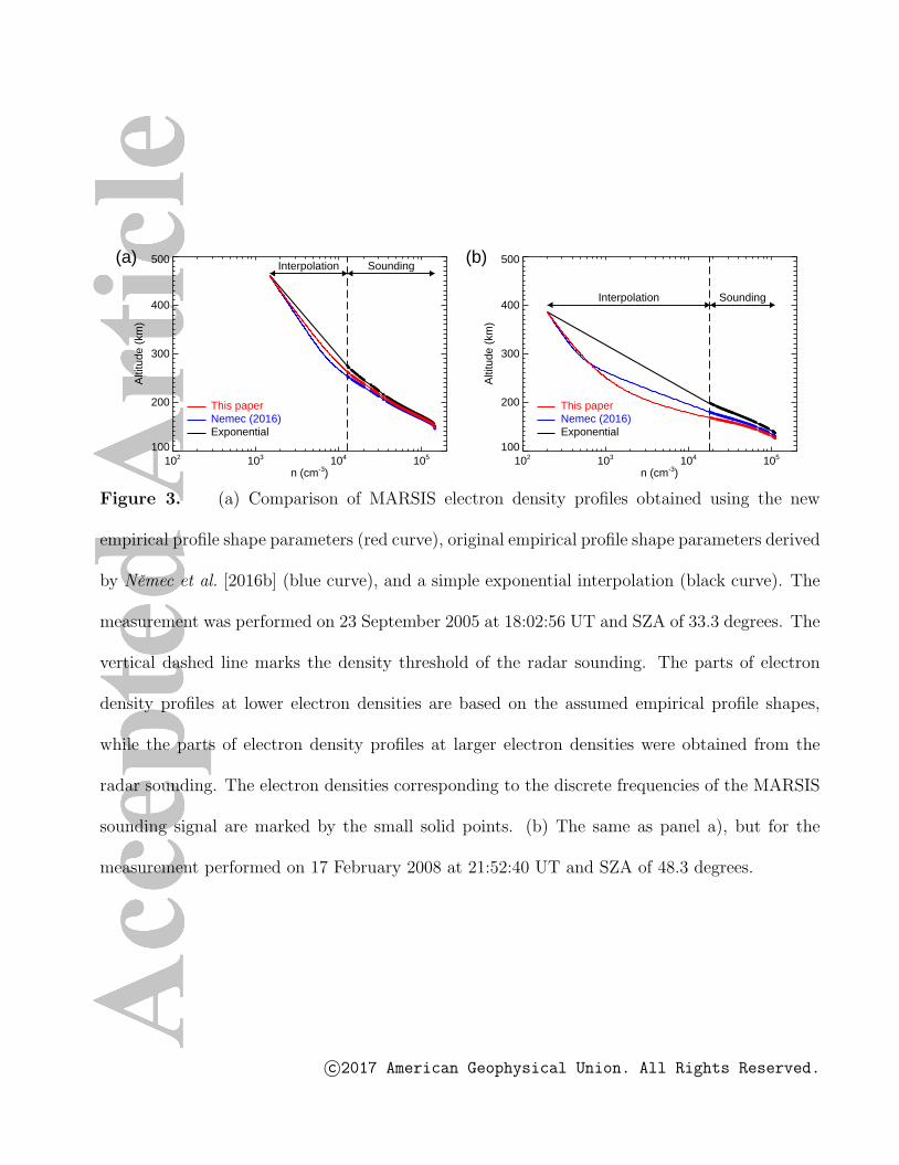
MARSIS electron density profiles. An example of a comparison between the electron
density profiles obtained using the old and new parameters is shown in Figure 3. Electron
density profiles based on the MARSIS measurements performed at two representative time
intervals are shown. Figure 3a was obtained using the data measured on 23 September
2005 at 18:02:56 UT and SZA of 33.3 degrees. The electron density profile obtained using
the parameters of the empirical profile shape derived in the present paper is shown by the
red curve. The electron density profile obtained using the original empirical profile shape
parameters derived by Nemec et al. [2016b] is shown by the blue curve. Finally, the black
curve shows the electron density profile obtained using a simple exponential interpolation.
It can be seen that the difference between the individual curves is not very large. This
is because the analyzed time interval corresponds to a situation of rather large electron
densities, when the altitude of the first data point available from the ionospheric sounding
is high as compared to the transition altitude. In such a case, only the high altitude
exponential part of the empirical profile is used, i.e., the method effectively converges to
a simple exponential interpolation.
Figure 3b obtained using the data measured on 17 February 2008 at 21:52:40 UT and
SZA of 48.3 degrees shows a rather different picture. In this case, the overall electron
densities are lower, and the first data point available from the ionospheric sounding is at a
c⃝2017 American Geophysical Union. All Rights Reserved.

rather low altitude, increasing thus the importance of a reasonable empirical profile shape
in the return signal gap region. It can be seen that the red curve represents arguably
the most realistic profile shape. Specifically, the transition altitude z0 = 275 km used by
Nemec et al. [2016b] appears to be too high. This is the case both when comparing with
the radio occultation results [Vogt et al., 2016] and with the recently available MARSIS
measurements, as well as with simple theoretical estimates based on the evaluation of
diffusive and photochemical time scales [Withers , 2009]. All these independent estimates
indicate that the transition altitude should be at about 200 km. We note that although
the shapes of electron density profiles at large electron densities (low altitudes) are not
too affected by an empirical profile shape assumed in the return signal gap region, all the
high density parts of the profiles may effectively shift in the altitude. The newly derived
parameters of the empirical electron density profile shape result in the peak altitude
difference generally within about 4 km (median −0.4 km, mean −0.6 km) as compared
to the original values derived by Nemec et al. [2016b]. Considering that the uncertainty
in the MARSIS ionospheric trace delay times corresponds to about 13.7 km [Morgan
et al., 2013], this difference in the determined peak altitudes is very small, and possibly
significant only when many traces are analyzed in a statistical manner. However, the
difference between the profiles at higher altitudes is progressively larger (see Figure 3b).
4. Coincident observations
Coincident MARSIS and LPW electron density measurements can be used to under-
stand how the data sets overlap, and to provide different views of the same ionosphere.
In order to do so, we would ideally need to select the time intervals when the spacecraft
were close to each other both in time and space. However, as this is very difficult to
c⃝2017 American Geophysical Union. All Rights Reserved.
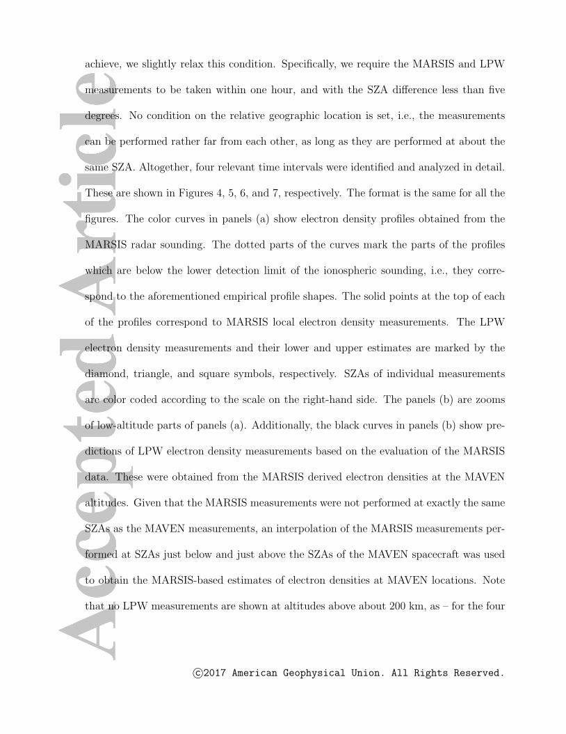
achieve, we slightly relax this condition. Specifically, we require the MARSIS and LPW
measurements to be taken within one hour, and with the SZA difference less than five
degrees. No condition on the relative geographic location is set, i.e., the measurements
can be performed rather far from each other, as long as they are performed at about the
same SZA. Altogether, four relevant time intervals were identified and analyzed in detail.
These are shown in Figures 4, 5, 6, and 7, respectively. The format is the same for all the
figures. The color curves in panels (a) show electron density profiles obtained from the
MARSIS radar sounding. The dotted parts of the curves mark the parts of the profiles
which are below the lower detection limit of the ionospheric sounding, i.e., they corre-
spond to the aforementioned empirical profile shapes. The solid points at the top of each
of the profiles correspond to MARSIS local electron density measurements. The LPW
electron density measurements and their lower and upper estimates are marked by the
diamond, triangle, and square symbols, respectively. SZAs of individual measurements
are color coded according to the scale on the right-hand side. The panels (b) are zooms
of low-altitude parts of panels (a). Additionally, the black curves in panels (b) show pre-
dictions of LPW electron density measurements based on the evaluation of the MARSIS
data. These were obtained from the MARSIS derived electron densities at the MAVEN
altitudes. Given that the MARSIS measurements were not performed at exactly the same
SZAs as the MAVEN measurements, an interpolation of the MARSIS measurements per-
formed at SZAs just below and just above the SZAs of the MAVEN spacecraft was used
to obtain the MARSIS-based estimates of electron densities at MAVEN locations. Note
that no LPW measurements are shown at altitudes above about 200 km, as – for the four
c⃝2017 American Geophysical Union. All Rights Reserved.
analyzed coincident events – these were measured at SZAs larger than 80 degrees, and
they thus do not meet the aforementioned selection criteria.
The data depicted in Figure 4 were obtained on 2 October 2015. The relevant MARSIS
data were obtained within a four minute interval between 00:36:11 UT and 00:40:20 UT.
The spacecraft latitude at this time interval was between −59.3◦ and −43.6◦, and the
spacecraft east longitude was between 116.9◦ and 118.1◦. The corresponding LPW elec-
tron density measurements were performed on the same day between 00:18:11 UT and
00:21:39 UT. The latitude of the MAVEN spacecraft at this time interval was between
−58.2◦ and −45.6◦, and the east longitude of the MAVEN spacecraft was between 115.3◦
and 124.9◦. The two spacecraft thus flew over the very same region, with a time delay
between MAVEN and Mars Express of about 20 minutes. The LPW electron density
measurements agree reasonably well with the MARSIS electron density profiles, but they
tend to be somewhat lower, with the MARSIS electron densities in between the LPW
electron densities and their upper estimates.
Figures 5 and 6 show roughly the same picture obtained for two other events. The first of
them occurred on 2 October 2015, with the MARSIS data measured between 14:35:15 UT
and 14:39:17 UT, and the LPW data measured between 13:57:10 UT and 14:00:34 UT. At
the given time interval, the Mars Express spacecraft was located at the latitude between
about −59.6◦ and −44.4◦. The east longitude of the spacecraft was between about 272.3◦
and 273.6◦. The MAVEN spacecraft at the time of the LPW measurements of interest
was located at the latitude between about −58.6◦ and −46.2◦ and east longitude between
about 275.7◦ and 285.4◦. This means that, again, the two spacecraft flew above nearly
the same region, with the MAVEN spacecraft being about 38 minutes ahead. The second
c⃝2017 American Geophysical Union. All Rights Reserved.

event occurred on 4 October 2015, with the MARSIS data measured between 01:33:52 UT
and 01:37:30 UT, and the LPW data measured between 02:19:53 UT and 02:22:57 UT.
At the time of the measurements, the Mars Express spacecraft was located at the latitude
between about −56.1◦ and −42.5◦ and east longitude between about 121.5◦ and 122.4◦.
At the time of the LPW measurements of interest, the MAVEN spacecraft was located at
the latitude between about −56.0◦ and −44.7◦ and east longitude between about 102.0◦
and 109.8◦. Although the the two spacecraft were thus separated by some 15 degrees
in longitude, they were still reasonably close to each other, with the MAVEN spacecraft
being by about 45 minutes ahead of Mars Express.
The event depicted in Figure 7 appears to result in the best overall agreement between
the MARSIS and LPW electron density measurements. It occurred on 6 October 2015,
with the MARSIS data measured between 09:29:33 UT and 09:33:27 UT, and the LPW
data measured between 08:55:55 UT and 08:59:15 UT. At the time of the measurements,
the MARSIS spacecraft was located at the latitude between about −58.9◦ and −44.3◦ and
east longitude between about 23.1◦ and 24.3◦. At the time of the LPW measurements of
interest, the MAVEN spacecraft was located at the latitude between about −58.5◦ and
−46.5◦ and east longitude between about 23.3◦ and 32.7◦. The two spacecraft thus flew
above approximately the same region, with the MAVEN spacecraft being some 35 minutes
ahead of Mars Express.
The overall agreement between the MARSIS and LPW electron density measurements
is analyzed in Figures 8 and 9. Figure 8 shows a direct comparison of LPW and MARSIS
electron density measurements (interpolated to the MAVEN SZAs, i.e., the black curves
from Figures 4, 5, 6, and 7). The lower and upper uncertainties of LPW electron density
c⃝2017 American Geophysical Union. All Rights Reserved.

measurements are shown by the vertical error bars. The SZAs of the MAVEN spacecraft
at the times of the measurements are color coded according to the scale on the right-hand
side. The diamond, triangle, square, and cross symbols correspond to the first, second,
third, and fourth event, respectively. The diagonal dashed line shows a 1:1 dependence.
It can be seen that the MARSIS and LPW electron densities agree remarkably well. The
large cluster of data points at larger electron densities is on average slightly below the
dashed line, corresponding to the MAVEN electron densities systematically somewhat
below the MARSIS electron densities, consistent with the aforementioned results. The
data points at low electron densities (< 104 cm−3) are below the detection threshold of
the MARSIS ionospheric sounding, i.e., the appropriate MARSIS electron densities were
obtained using the empirical electron density profile shape smoothly transiting between
the locally measured electron density at the Mars Express spacecraft location and the
first data point from the MARSIS ionospheric sounding.
A histogram of the ratios between the LPW and MARSIS electron densities is shown
in Figure 9 by the black line. The blue and red lines show, respectively, the histograms
obtained using the LPW lower and upper electron density estimates. The vertical dashed
lines of respective colors correspond to appropriate median values. The LPW electron
densities are on average somewhat lower than those determined using the MARSIS data
(median electron density ratio of about 0.73). However, considering the lower and upper
uncertainties of the LPW measurements, the two data sets are well consistent (median
ratio value obtained using the LPW lower electron density estimates is about 0.43, median
ratio value obtained using the LPW upper electron density estimates is about 1.44).
c⃝2017 American Geophysical Union. All Rights Reserved.

5. Discussion
The low power radiated by the MARSIS radar sounder at low sounding frequencies and
the associated return signal gap represent a considerable complication when performing
the trace inversion, i.e., when recalculating the measured ionospheric traces into electron
density profiles. Specifically, electron density profiles in the density range between the
local electron density and the lowest electron density detectable by the ionospheric sound-
ing cannot be deduced using the MARSIS data. The inversion of MARSIS ionospheric
traces is thus ambiguous. Moreover, considering the dispersion of the sounding signal,
the ambiguity concerns not only the low-density parts of electron density profiles, but ef-
fectively affects the entire profile. Although the profile shape at higher electron densities
(low altitudes) is not very sensitive to the exact choice of the electron profile shape in the
return signal gap region, the profile as a whole can effectively move to higher/lower alti-
tudes by as much as five km. At higher altitudes (lower electron densities) the difference
is generally larger (see Figure 3). As the primary purpose of the MARSIS radar sounding
is to obtain electron density profiles, and the large amount of MARSIS radar sounding
data collected to date is used to construct/validate models and statistics of the Martian
ionospheric electron densities [Morgan et al., 2008; Nemec et al., 2011; Sanchez-Cano
et al., 2013], it is important to tune the inversion procedure to obtain as reliable electron
density profiles as possible. This is particularly striking when analyzing the MARSIS
electron density profiles in a statistical manner, as unrealistic profile shapes in the return
signal gap region may result in a systematic bias in derived altitudes Nemec et al. [2016b].
The formerly considered unrealistic profile shapes are also a reason for the discrepancies
c⃝2017 American Geophysical Union. All Rights Reserved.

between MARSIS and radio occultation electron density data sets reported by Vogt et al.
[2016] at higher altitudes.
It is thus of the utmost importance to estimate the profile shape in the return signal
gap region as well as possible. The profile shape suggested by Nemec et al. [2016b] and
the related trace inversion routine respects long-term statistical dependencies derived for
the high-altitude diffusion region, and, moreover, it can be easily used for the inversion
of MARSIS ionospheric traces. The two parameters describing the profile shape in this
region, namely the transition altitude z0 and the radius of curvature δ, cannot be directly
determined using the MARSIS data. However, the availability of the MAVEN LPW
electron density data allowed for their direct evaluation. We determined the optimal
values of these parameters in such a way that the resulting empirical electron density
profiles closely follow the long-term LPW dependencies. The used approach demonstrates
clearly the advantage of using the LPW electron density data set along with the MARSIS
measurements. We note that the revised trace inversion routine based on the LPW-
determined parameters is on average optimal, in the sense that the obtained results follow
the expected long-term distributions. Nevertheless, in individual cases, the actual profile
shapes in the return signal gap region may differ significantly from the long-term average,
and the used trace inversion routine would thus result in not entirely correct electron
density profiles. This is a principal limitation stemming from the MARSIS data, and it
cannot be overcome.
It is important to perform a direct comparison of LPW and MARSIS electron densities,
in order to verify their correctness and identify any possible biases. Given that the in-
struments orbit on two different spacecraft, it is principally impossible for them to occur
c⃝2017 American Geophysical Union. All Rights Reserved.

at exactly the same location. However, considering that SZA and the incoming solar ra-
diation flux are the most important controlling factors of the Martian daytime ionosphere
[e.g. Withers , 2009; Nemec et al., 2011], we can focus on the analysis of the time intervals
when the spacecraft are located at about the same SZAs. The approximately same times
of the measurements then ensure that the solar radiation flux and the Sun-Mars distance
are basically the same. However, the spacecraft may be located at different geographic
locations, with different local conditions and with different configuration and magnitude
of the crustal magnetic fields.
Nevertheless, the LPW electron densities are in agreement with the MARSIS electron
densities in all analyzed coincident events. They are on average somewhat lower than the
MARSIS electron densities, but the difference is well within the uncertainty range. Apart
from the Langmuir probe measurements, there are also other measurements on board
MAVEN which can be used to derive plasma densities, such as the waves measurements,
neutral gas and ion mass spectrometer, and the low energy ion detector. All these suggest
that at high densities the Langmuir probe measurements are on the high density ends.
We note in this regard that it is difficult to evaluate the uncertainty of the MARSIS
electron density measurements. Due to the inversion process and the necessity to derive
the corrected altitude range, the uncertainty of the resulting electron density profiles is
primarily altitudinal. Should the possible overestimation of MARSIS electron densities as
compared to the LPW measurements be a MARSIS issue, it would thus likely correspond
to MARSIS electron density profiles being on average slightly “too high”, i.e., with the
assumed electron density profile shape in the return signal gap region not steep enough.
c⃝2017 American Geophysical Union. All Rights Reserved.

Although the assumed profile shape corresponds to the long-term average, it is possible
that in the few analyzed events the situation was rather different.
The observed differences between LPW in-situ electron density measurements and
MARSIS electron density profiles vary significantly from event to event and as a function
of the altitude. This remains the case even when the effect of the LPW measurements
being made at different SZAs is taken into account, as presented in Figures 4–7 when
comparing the black curves with the diamonds. However, the discrepancies observed in
Figures 4–7 are typically within the uncertainty in the LPW measurements. Considering
that LPW and MARSIS are two different instruments with completely different physical
principles placed on board two different spacecraft, the overall agreement of the measured
electron densities is surprisingly good.
6. Conclusions
We have presented the first direct comparison of electron density measurements in the
Martian ionosphere performed by the MARSIS instrument on board the Mars Express
spacecraft and by the LPW instrument on board the MAVEN spacecraft, demonstrating
a reasonable agreement between the two data sets. The in-situ measured LPW electron
densities were also used to improve the empirical profile shape in the altitudinal region not
covered by the MARSIS data, allowing to obtain more reliable MARSIS electron density
profiles.
Due to the low power radiated by the MARSIS radar sounder at low frequencies, it is
generally not possible to evaluate the low density parts of electron density profiles from
the measured data. Instead, one needs to assume a reasonable electron density profile
shape in the return signal gap region between the local electron density and the lowest
c⃝2017 American Geophysical Union. All Rights Reserved.

electron density detectable by the radar sounding. We demonstrated that the MAVEN
LPW electron density measurements can be efficiently used to determine an optimal shape
of this electron density profile. Although a significant morning-afternoon asymmetry was
identified in the MAVEN LPW data set, the return signal gap region can be described by
a single formula. We derived the values of its parameters, and we used the revised trace
inversion procedure to improve the accuracy of the MARSIS electron density profiles.
We further focused on a direct comparison between the MARSIS and LPW electron
densities during coincident events. Four events when the Mars Express and MAVEN
spacecraft were within a five degree SZA interval during a one hour time interval were
identified and analyzed. We showed that there is a good agreement between the electron
density measurements performed by the two instruments. The MAVEN electron densities
are typically slightly lower than those obtained by MARSIS, but within the uncertainties.
The obtained results allow us to improve the precision of the electron density profiles
obtained by the MARSIS instrument on board Mars Express. The calculated electron
densities are in agreement with the electron densities measured locally by the LPW in-
strument on board the MAVEN spacecraft. Further, preferentially large-scale, intercom-
parison between various electron density data sets is surely desirable, as it would allow
both to evaluate possible biases in individual instrument data and to better understand
the ionospheric variability. Given the ionospheric variability as a function of – among
others – the solar cycle, solar longitude, SZA, and location, and uncertainties in the ab-
solute density of the in-situ measurements and the altitude determined from the remote
sounding, it may be, however, difficult to achieve.
c⃝2017 American Geophysical Union. All Rights Reserved.
Acknowledgments. MARSIS data are available via the ESA Planetary Science
Archive (http://www.rssd.esa.int/PSA). MAVEN LPW data are available via the
Planetary Data System (https://pds-ppi.igpp.ucla.edu/). FN acknowledges the sup-
port of the MSMT INTER-ACTION grant LTAUSA17070.
References
Andersson, L., R. E. Ergun, G. T. Delory, A. Eriksson, J. Westfall, H. Reed, J. McCauly,
D. Summers, and D. Meyers (2015), The langmuire probe and waves (LPW) instrument
for MAVEN, SSR, 195, 173–198, doi:10.1007/s11214-015-0194-3.
Andrews, D. J., H. J. Opgenoorth, N. J. T. Edberg, M. Andre, M. Franz, E. Dubinin,
F. Duru, D. Morgan, and O. Witasse (2013), Determination of local plasma densities
with the MARSIS radar: Asymmetries in the high-altitude Martian ionosphere, J.
Geophys. Res. Space Physics, 118, 6228–6242, doi:10.1002/jgra.50593.
Andrews, D. J., N. J. T. Edberg, A. I. Eriksson, D. A. Gurnett, D. Morgan, F. Nemec, and
H. J. Opgenoorth (2015), Control of the topside Martian ionosphere by crustal magnetic
fields, J. Geophys. Res. Space Physics, 120, 3042–3058, doi:10.1002/2014JA020703.
Benna, M., P. R. Mahaffy, J. M. Grebowsky, J. L. Fox, R. V. Yelle, and B. M. Jakosky
(2015), First measurements of composition and dynamics of the Martian ionosphere
by MAVEN’s Neutral Gas and Ion Spectrometer, Geophys. Res. Lett., 42, doi:10.1007/
s11214-006-9124-8.
Chapman, S. (1931a), The absorption and dissociative or ionizing effect of monochromatic
radiation in an atmosphere on a rotating Earth, Proceedings of the Physical Society, 43,
26–45.
c⃝2017 American Geophysical Union. All Rights Reserved.

Chapman, S. (1931b), The absorption and dissociative or ionizing effect of monochromatic
radiation in an atmosphere on a rotating Earth, Part II. Grazing incidence, Proceedings
of the Physical Society, 43, 483–501.
Duru, F., D. A. Gurnett, D. D. Morgan, R. Modolo, A. F. Nagy, and D. Najib (2008),
Electron densities in the upper ionosphere of Mars from the excitation of electron plasma
oscillations, J. Geophys. Res., 113 (A07302), doi:10.1029/2008JA013073.
Duru, F., D. D. Morgan, and D. A. Gurnett (2010), Overlapping ionospheric and sur-
face echoes observed by the Mars Express radar sounder near the martian terminator,
Geophys. Res. Lett., 37 (L23102), doi:10.1029/2010GL045859.
Duru, F., D. A. Gurnett, D. D. Morgan, J. D. Winningham, R. A. Frahm, and A. F.
Nagy (2011), Nightside ionosphere of Mars studied with local electron densities: A
general overview and electron density depressions, J. Geophys. Res., 116 (A10316), doi:
10.1029/2011JA016835.
Ergun, R. E., M. W. Morooka, L. A. Andersson, C. M. Fowler, G. T. Delory, D. J.
Andrews, A. I. Eriksson, T. McEnulty, and B. M. Jakosky (2015), Dayside electron
temperature and density profiles at Mars: First results from the MAVEN langmuir probe
and waves instrument, Geophys. Res. Lett., 42, 8846–8853, doi:10.1002/2015GL065280.
Fowler, C. M., L. Andersson, J. Halekas, J. R. Espley, C. Mazelle, E. R. Coughlin, R. E.
Ergun, D. J. Andrews, J. E. P. Connerney, and B. Jakosky (2017), Electric and magnetic
variations in the near-Mars environment, J. Geophys. Res. Space Physics, 122, doi:
10.1002/2016JA023411.
Fox, J. L., and K. E. Yeager (2006), Morphology of the near-terminator Martian iono-
sphere: A comparison of models and data, J. Geophys. Res., 120, 6707–6721, doi:
c⃝2017 American Geophysical Union. All Rights Reserved.

10.1002/2014JA020947.
Girazian, Z., and P. Withers (2013), The dependence of peak electron density in the
ionosphere of Mars on solar irradiance, Geophys. Res. Lett., 40, 1960–1964, doi:10.
1002/grl.50344.
Gurnett, D. A., D. L. Kirchner, R. L. Huff, D. D. Morgan, A. M. Persoon, T. F. Averkamp,
F. Duru, E. Nielsen, A. Safaeinili, J. J. Plaut, and G. Picardi (2005), Radar soundings
of the ionosphere of Mars, Science, 310, 1929–1933, doi:10.1126/science.1121868.
Gurnett, D. A., R. L. Huff, D. D. Morgan, A. M. Persoon, T. F. Averkamp, D. L. Kirchner,
F. Duru, F. Akalin, A. J. Kopf, E. Nielsen, A. Safaeinili, J. J. Plaut, and G. Picardi
(2008), An overview of radar soundings of the martian ionosphere from the Mars Express
spacecraft, Adv. Space Res., 41, 1335–1346.
Gurnett, D. A., D. D. Morgan, F. Duru, F. Akalin, D. Winningham, R. A. Frahm,
E. Dubinin, and S. Barabash (2010), Large density fluctuations in the martian iono-
sphere as observed by the Mars Express radar sounder, Icarus, 206 (1), 83–94, doi:
10.1016/j.icarus.2009.02.019.
Jakosky, B. M., R. P. Lin, J. M. Grebowsky, J. G. Luhmann, D. F. Mitchell, G. Beu-
telschies, T. Priser, M. Acuna, L. Andersson, D. Baird, D. Baker, R. Bartlett, M. Benna,
S. Bougher, D. Brain, D. Carson, S. Cauffman, P. Chamberlin, J.-Y. Chaufray,
O. Cheatom, J. Clarke, J. Connerney, T. Cravens, D. Curtis, G. Delory, S. Demcak,
A. DeWolfe, F. Eparvier, R. Ergun, A. Eriksson, J. Espley, X. Fang, D. Folta, J. Fox,
C. Gomez-Rosa, S. Habenicht, J. Halekas, G. Holsclaw, M. Houghton, R. Howard,
M. Jarosz, N. Jedrich, M. Johnson, W. Kasprzak, M. Kelley, T. King, M. Lankton,
D. Larson, J. McFadden, D. L. Mitchell, F. Montmessin, J. Morrissey, W. Peterson,
c⃝2017 American Geophysical Union. All Rights Reserved.

W. Possel, J.-A. Sauvaud, N. Schneider, W. Sidney, S. Sparacino, A. I. F. Stewart,
R. Tolson, D. Toublanc, C. Waters, T. Woods, R. Yelle, and R. Zurek (2015), The Mars
Atmosphere and Volatile Evolution (MAVEN) mission, Space Sci. Rev., 195 (1), 3–48,
doi:10.1007/s11214-015-0139-x.
Jordan, R., G. Picardi, J. Plaut, K. Wheeler, D. Kirchner, A. Safaeinili, W. Johnson,
R. Seu, D. Calabrese, E. Zampolini, A. Cicchetti, R. Huff, D. Gurnett, A. Ivanov,
W. Kofman, R. Orosei, T. Thompson, P. Edenhofer, and O. Bombaci (2009), The
Mars Express MARSIS sounder instrument, Planet. Space Sci., 57, 1975–1986, doi:
10.1016/j.pss.2009.09.016.
Kim, E., H. Seo, J. H. Kim, J. H. Lee, Y. H. Kim, G.-H. Choi, and E.-S. Sim (2012),
The analysis of the topside additional layer of Martian ionosphere using MARSIS/Mars
Express data, J. Astron. Space Sci., 29 (4), 337–342, doi:10.5140/JASS.2012.29.4.337.
Kopf, A. J., D. A. Gurnett, D. D. Morgan, and D. K. Kirchner (2008), Transient
layers in the topside ionosphere of Mars, Geophys. Res. Lett., 35 (L17102), doi:
10.1029/2008GL034948.
Mendillo, M., A. G. Marusiak, P. Withers, D. Morgan, and D. Gurnett (2013), A new
semiempirical model of the peak electron density of the Martian ionosphere, Geophys.
Res. Lett., 40, 1–5, doi:10.1002/2013GL057631.
Morgan, D. D., D. A. Gurnett, D. L. Kirchner, J. L. Fox, E. Nielsen, and J. J. Plaut
(2008), Variation of the Martian ionospheric electron density from Mars Express radar
soundings, J. Geophys. Res., 113 (A09303), doi:10.1029/2008JA013313.
Morgan, D. D., O. Witasse, E. Nielsen, D. A. Gurnett, F. Duru, and D. L. Kirchner
(2013), The processing of electron density profiles from the Mars Express MARSIS
c⃝2017 American Geophysical Union. All Rights Reserved.

topside sounder, Radio Sci., 48 (3), 197–207, doi:10.1002/rds.20023.
Nemec, F., D. D. Morgan, D. A. Gurnett, and F. Duru (2010), Nightside ionosphere of
Mars: Radar soundings by the Mars Express spacecraft, J. Geophys. Res., 115 (E12009),
doi:10.1029/2010JE003663.
Nemec, F., D. D. Morgan, D. A. Gurnett, F. Duru, and V. Truhlık (2011), Dayside
ionosphere of Mars: Empirical model based on data from the MARSIS instrument, J.
Geophys. Res., 116 (E07003), doi:10.1029/2010JE003789.
Nemec, F., D. D. Morgan, D. A. Gurnett, and D. J. Andrews (2016a), Empirical model
of the Martian dayside ionosphere: Effects of crustal magnetic fields and solar ionizing
flux at higher altitudes, J. Geophys. Res. Space Physics, 121, 1760–1771, doi:10.1002/
2015JA022060.
Nemec, F., D. D. Morgan, and D. A. Gurnett (2016b), On improving the accuracy of
electron density profiles obtained at high altitudes by the ionospheric sounder on the
Mars Express spacecraft, J. Geophys. Res. Space Physics, 121, 10,117–10,129, doi:10.
1002/2016JA023054.
Picardi, G., D. Biccari, R. Seu, J. Plaut, W. T. K. Johnson, R. L. J. A. Safaeinili, D. A.
Gurnett, R. Huff, R. Orosei, O. Bombaci, D. Calabrese, and E. Zampolini (2004),
MARSIS: Mars advanced radar for subsurface and ionosphere sounding, in Mars Ex-
press: the Scientific Payload, ESA Special Publication, vol. 1240, edited by A. Wilson
and A. Chicarro, pp. 51–69.
Sanchez-Cano, B., S. M. Radicella, M. Herraiz, O. Witasse, and G. Rodrıguez-Caderot
(2013), NeMars: An empirical model of the martian dayside ionosphere based on Mars
Express MARSIS data, Icarus, 225, 236–247, doi:10.1016/j.icarus.2013.03.021.
c⃝2017 American Geophysical Union. All Rights Reserved.

Vogt, M. F., P. Withers, K. Fallows, C. L. Flynn, D. J. Andrews, F. Duru, and D. D.
Morgan (2016), Electron densities in the ionosphere of Mars: A comparison of MARSIS
and radio occultation measurements, J. Geophys. Res. Space Physics, 121, 10,241–
10,257, doi:10.1002/2016JA022987.
Wang, X.-D., J.-S. Wang, and H. Zou (2012), On the small-scale fluctuations in the peak
electron density of Martian ionosphere observed by MEX/MARSIS, Planet. Space Sci.,
63–64, 87–93, doi:10.1016/j.pss.2011.10.007.
Withers, P. (2009), A review of observed variability in the dayside ionosphere of Mars,
Adv. Space Res., 44, 277–3078, doi:10.1016/j.asr.2009.04.027.
Withers, P., K. Fallows, Z. Girazian, M. Matta, B. Hausler, D. Hinson, L. Tyler, D. Mor-
gan, M. Patzold, K. Peter, S. Tellmann, J. Peralta, and O. Witasse (2012a), A clear
view of multifaceted dayside ionosphere of Mars, Geophys. Res. Lett., 39 (L18202), doi:
10.1029/2012GL053193.
Withers, P., M. O. Fillingim, R. J. Lillis, B. Hausler, D. P. Hinson, G. L. Tyler, M. Patzold,
K. Peter, S. Tellmann, and O. Witasse (2012b), Observations of the nightside ionosphere
of Mars by the Mars Express Radio Science Experiment (MaRS), J. Geophys. Res.,
117 (A12307), doi:10.1029/2012JA018185.
c⃝2017 American Geophysical Union. All Rights Reserved.

(a) (b)
100 1000 10000n (cm-3)
150
200
250
300
Alti
tude
(km
)
0o < SZA < 30o
"morning"
100 1000 10000n (cm-3)
150
200
250
300
Alti
tude
(km
)
30o < SZA < 50o
"morning"
0.00
0.02
0.04
0.06
0.08
0.10
0.12
0.14
Pro
babi
lity
of m
easu
ring
a de
nsity
at a
n al
titud
e
(c) (d)
100 1000 10000n (cm-3)
150
200
250
300
Alti
tude
(km
)
50o < SZA < 60o
"morning"
100 1000 10000n (cm-3)
150
200
250
300
Alti
tude
(km
)
60o < SZA < 70o
"morning"
0.00
0.02
0.04
0.06
0.08
0.10
0.12
0.14
Pro
babi
lity
of m
easu
ring
a de
nsity
at a
n al
titud
e
(e) (f)
100 1000 10000n (cm-3)
150
200
250
300
Alti
tude
(km
)
70o < SZA < 80o
"morning"
100 1000 10000n (cm-3)
150
200
250
300
Alti
tude
(km
)
80o < SZA < 90o
"morning"
0.00
0.02
0.04
0.06
0.08
0.10
0.12
0.14
Pro
babi
lity
of m
easu
ring
a de
nsity
at a
n al
titud
e
Figure 1. (a)–(f) Probability of LPW measuring an electron density in a given density bin at a givenaltitude is color coded according to the color scale on the right-hand side. Only measurements at MSOlocal times 6–12 hours were used. The thick black curves show the median altitudinal dependencies ofthe electron density. The white curves show the empirical fits using the hyperbola transition betweentwo exponential dependencies (see text). Individual panels were obtained for different SZA intervals.These are stated at the top left of each of the panels.
c⃝2017 American Geophysical Union. All Rights Reserved.

(a) (b)
100 1000 10000n (cm-3)
150
200
250
300
Alti
tude
(km
)
0o < SZA < 30o
"afternoon"
100 1000 10000n (cm-3)
150
200
250
300
Alti
tude
(km
)
30o < SZA < 50o
"afternoon"
0.00
0.02
0.04
0.06
0.08
0.10
0.12
0.14
Pro
babi
lity
of m
easu
ring
a de
nsity
at a
n al
titud
e
(c) (d)
100 1000 10000n (cm-3)
150
200
250
300
Alti
tude
(km
)
50o < SZA < 60o
"afternoon"
100 1000 10000n (cm-3)
150
200
250
300
Alti
tude
(km
)
60o < SZA < 70o
"afternoon"
0.00
0.02
0.04
0.06
0.08
0.10
0.12
0.14
Pro
babi
lity
of m
easu
ring
a de
nsity
at a
n al
titud
e
(e) (f)
100 1000 10000n (cm-3)
150
200
250
300
Alti
tude
(km
)
70o < SZA < 80o
"afternoon"
100 1000 10000n (cm-3)
150
200
250
300
Alti
tude
(km
)
80o < SZA < 90o
"afternoon"
0.00
0.02
0.04
0.06
0.08
0.10
0.12
0.14
Pro
babi
lity
of m
easu
ring
a de
nsity
at a
n al
titud
e
Figure 2. The same as Figure 1, but for the MSO local times 12–18 hours.
c⃝2017 American Geophysical Union. All Rights Reserved.
(a) (b)
102 103 104 105
n (cm-3)
100
200
300
400
500
Alti
tude
(km
)
Interpolation Sounding
This paperNemec (2016)Exponential
102 103 104 105
n (cm-3)
100
200
300
400
500
Alti
tude
(km
)
Interpolation Sounding
This paperNemec (2016)Exponential
Figure 3. (a) Comparison of MARSIS electron density profiles obtained using the new
empirical profile shape parameters (red curve), original empirical profile shape parameters derived
by Nemec et al. [2016b] (blue curve), and a simple exponential interpolation (black curve). The
measurement was performed on 23 September 2005 at 18:02:56 UT and SZA of 33.3 degrees. The
vertical dashed line marks the density threshold of the radar sounding. The parts of electron
density profiles at lower electron densities are based on the assumed empirical profile shapes,
while the parts of electron density profiles at larger electron densities were obtained from the
radar sounding. The electron densities corresponding to the discrete frequencies of the MARSIS
sounding signal are marked by the small solid points. (b) The same as panel a), but for the
measurement performed on 17 February 2008 at 21:52:40 UT and SZA of 48.3 degrees.
c⃝2017 American Geophysical Union. All Rights Reserved.

102 103 104 105
n (cm-3)
100
200
300
400
500
Alti
tude
(km
)
MARSIS localMARSIS gapMARSIS soundingMAVEN mainMAVEN lowerMAVEN upper
66687072747678
SZ
A (
deg)
(a)
103 104 105
n (cm-3)
140
160
180
200
Alti
tude
(km
)
66687072747678
SZ
A (
deg)
(b)
Figure 4. (a) The color curves show electron density profiles obtained by the MARSIS instrument on2 October 2015 between 00:36:11 UT and 00:40:20 UT. The dotted parts of curves mark the parts of theelectron density profiles not accessible by the ionospheric sounding, i.e., based on the empirical electrondensity profile shape. The solid parts of the curves mark the parts of the electron density profilesdetermined from the ionospheric sounding. The solid points at the top of each of the profiles correspondto MARSIS local electron density measurements. SZAs of individual electron density profiles are colorcoded according to the color scale on the right-hand side. The color diamonds, triangles, and squarescorrespond to LPW electron density measurements and their lower and upper uncertainty estimates,respectively. These were obtained on 2 October 2015 between 00:18:11 UT and 00:21:39 UT. Theappropriate SZAs are again color coded according to the color scale on the right-hand side. (b) A zoomof the low-altitude part of the top panel. The used format is the same. Additionally, the black curveshows a prediction of the LPW electron density measurements based on the MARSIS data.
c⃝2017 American Geophysical Union. All Rights Reserved.

102 103 104 105
n (cm-3)
100
200
300
400
500
Alti
tude
(km
)
MARSIS localMARSIS gapMARSIS soundingMAVEN mainMAVEN lowerMAVEN upper
66687072747678
SZ
A (
deg)
(a)
103 104 105
n (cm-3)
140
160
180
200
Alti
tude
(km
)
66687072747678
SZ
A (
deg)
(b)
Figure 5. The same as Figure 4, but for MARSIS measurements on 2 October 2015 between
14:35:15 UT and 14:39:16 UT and LPW measurements on 2 October 2015 between 13:57:10 UT
and 14:00:34 UT.
c⃝2017 American Geophysical Union. All Rights Reserved.

102 103 104 105
n (cm-3)
100
200
300
400
500
Alti
tude
(km
)
MARSIS localMARSIS gapMARSIS soundingMAVEN mainMAVEN lowerMAVEN upper
66687072747678
SZ
A (
deg)
(a)
103 104 105
n (cm-3)
140
160
180
200
Alti
tude
(km
)
66687072747678
SZ
A (
deg)
(b)
Figure 6. The same as Figure 4, but for MARSIS measurements on 4 October 2015 between
01:33:52 UT and 01:37:30 UT and LPW measurements on 4 October 2015 between 02:19:53 UT
and 02:22:57 UT.
c⃝2017 American Geophysical Union. All Rights Reserved.

102 103 104 105
n (cm-3)
100
200
300
400
500
Alti
tude
(km
)
MARSIS localMARSIS gapMARSIS sounding
MAVEN mainMAVEN lowerMAVEN upper
66687072747678
SZ
A (
deg)
(a)
103 104 105
n (cm-3)
140
160
180
200
Alti
tude
(km
)
66687072747678
SZ
A (
deg)
(b)
Figure 7. The same as Figure 4, but for MARSIS measurements on 6 October 2015 between
09:29:33 UT and 09:33:27 UT and LPW measurements on 6 October 2015 between 08:55:55 UT
and 08:59:15 UT.
c⃝2017 American Geophysical Union. All Rights Reserved.

103 104 105
nMARSIS (cm-3)
103
104
105
n MA
VE
N (
cm-3)
66
68
70
72
74
76
78
SZ
A (
deg)
Figure 8. Electron densities measured by the LPW instrument as a function of corresponding
electron densities evaluated for the appropriate altitudes and SZAs based on the MARSIS electron
density profiles. The vertical error bars show the uncertainties of the LPW electron density
measurements. The data points corresponding to the events from Figures 4, 5, 6, and 7 are
shown by the diamonds, triangles, squares, and crosses, respectively. The color of individual
symbols corresponds to the SZA of the measurements, using the color scale on the right-hand
side.
c⃝2017 American Geophysical Union. All Rights Reserved.

0.1 1.0 10.0nMAVEN / nMARSIS
0
20
40
60
80
Num
ber
of D
ata
Poi
nts
MAVEN lowerMAVEN mainMAVEN upper
Figure 9. Histogram of the ratios between LPW electron densities and corresponding electron
densities evaluated for the appropriate altitudes and SZAs based on the MARSIS electron density
profiles. The blue, black, and red histograms were obtained using LPW lower electron density
estimates, main electron density estimates, and upper electron density estimates, respectively.
The color vertical dashed lines mark the median values of the respective distributions.
c⃝2017 American Geophysical Union. All Rights Reserved.