Investment Reluctance: Irreversibility or Imperfect Capital Markets? Evidence from German Farm Panel Data
Preliminary version - please contact before quoting.
Silke Hüttel a*, Oliver Mußhoff b, Martin Odening † a
a Humboldt University Berlin, Faculty of Agriculture and Horticulture, Farm Management Group
b Martin-Luther-University Halle-Wittenberg, Institute of Agricultural and Nutritional Sciences, Farm Management Group
*Correspondence: Luisenstraße 56, D-10099 Berlin, Germany. Phone: +49-30-2093-6459, fax: +49-30-2093-6465,
e-mail: [email protected]
Selected Paper prepared for presentation at the American Agricultural Economics Association Annual Meeting, Portland, OR, July 29 – August 1, 2007
Copyright 2007 by [Silke Hüttel, Oliver Mußhoff, Martin Odening]. All rights reserved. Readers may verbatim copies of this document for non-commercial purposes by any means, provided that this copyright notice appears on all such copies.
† The authors gratefully acknowledge financial support from the German Research Foundation (DFG).
Abstract
Investment behavior at the firm level is characterized by lumpy adjustments and frequent
periods of inactivity. Low investment rates are particularly puzzling in transition
economies where an urgent need of modernization exists. The literature offers two
explanations for. Firstly, neo-institutional finance theory focuses on the impacts of
imperfect capital markets on investment decisions showing that the limited availability of
financial funds may confine firms’ investments. Secondly, real options theory asserts that
the interaction of irreversibility, uncertainty and flexibility may also result in investment
reluctance. In this paper we suggest a generalized model that combines imperfect capital
markets and real options effects. We also offer an econometric implementation that has
the structure of a generalized tobit model. This model is applied to German farm panel
data. We demonstrate that ignoring real options effects may lead to erroneous results
when estimating the impact of imperfect capital markets on investment decisions.
Keywords: investment decision; irreversibility; uncertainty; q-model; capital market
imperfections; generalized tobit model; transition
JEL classification: D81; D92; O12
2
Observed investment behavior at the firm level is characterized by lumpy investments and
frequent periods of inactivity. Low investment rates are particularly puzzling in transition
economies where an urgent need of modernization and rationalization exists. Numerous
studies have already tried to provide a better understanding of firm-level investment
pointing out the important role of finance (amongst others, BOND and MEGHIR 1994;
GILCHRIST and HIMMELBERG 1998 and for agricultural investment e.g., BENJAMIN and
PHIMISTER 2002; BARRY, BIERLEN and SOTOMAYOR 2000). As imperfect capital markets
are characterized by informational asymmetries and agency problems induce transaction
costs, a gap between firms’ cost for internal and external finance arises. Henceforth,
investment and finance decisions are not separate1. This is in particular the case in
transition economies where underdeveloped institutions and weak macroeconomic
conditions lead even to constrained capital access (amongst others, PAVEL , SHERBAKOV
and VERSTYUK 2004; RIZOV 2004). The aforementioned empirical studies affirm a direct
effect of imperfect capital markets. Therefore, the well known standard investment model
with strictly convex costs attached to adjusting the capital stock is extended by imposing
financial restrictions in order to account for costly or limited access to capital.
Accordingly, investment is sensitive to the cash flow as a proxy for internal financial
ability (BOND and VAN REENEN 2003).
However, the extended standard investment model fails to explain observed lumpy
investment (CHIRINKO 1993). An alternative explanation of investment reluctance is
offered by the real options theory, that has a close relationship to the stochastic
adjustment cost theory. Real options theory affirms that inaction periods occur when costs
for the adjustment of the capital stock are at least partially sunken (irreversible) and
future revenues are uncertain. Costly reversibility arises when installing new capital
1 HUBBARD (1998) gives a comprehensive review about imperfect capital markets.
3
involves costly learning or disruption costs, or alternatively when high capital specificity
leads to a lack of resale possibilities. Of particular interest is the interaction of
uncertainty, irreversibility and the opportunity to postpone investment (DIXIT and
PINDYCK 1994). This means, investment is influenced by the value of the real option to
invest and delaying investment might become optimal. In this context, a more general
form of the adjustment cost function is required in order to account for irreversibility
(HAMERMESH and PFANN 1996). It is assumed that these costs are asymmetric, only
partially convex and kinked at zero investment (CABALLERO 1997). The resulting optimal
path of investment depending on the marginal valuation of capital is non-smooth and
characterized by a range of inaction. For instance ABEL and EBERLY (2002), NILSEN and
SCHIANTARELLI (2003) or LETTERIE and PFANN (2007) give empirical evidence about
asymmetric adjustments of the capital stock.
This study strongly recommends that imperfect capital markets inducing additional
transaction costs are a major determinant of investments. In transition economies these
effects are expected to be even more pronounced as weak macroeconomic conditions
hinder the development of capital markets. However, impacts of imperfect capital market
cannot solely explain empirical investment behavior characterized by reluctance. We aim
to advance the understanding of investment behavior and endorse that costly reversibility
and uncertain future expectations are major determinants along with the availability of
finance. Thus, we combine issues of two strands of investment literature – the neo-
institutional finance theory and the real options theory. To our knowledge do empirical
applications so far not provide any bridging application. Accordingly, this is the
innovative part and the main contribution of this study as more recent papers do not
combine these aspects (LENSINK and BO 2001).
4
For these purposes we develop an extended q-model with the intention of exploring the
coexistence of capital market imperfections, irreversibility and uncertainty referring to
ABEL and EBERLY (1994). The empirical model has the structure of a generalized tobit
model. By means of this model we intend to show that simpler linear models, assuming a
smooth adjustment of the capital stock over time, fail to explain empirical investment
behavior when capital market imperfections, costly reversibility and uncertainty coexist.
The application of this model to German farm level panel data aims to investigate first, if
and how imperfect capital markets, irreversibility and uncertainty jointly affect empirical
farm investment behavior. The second objective is to substantiate if farms in transition
economies are confronted with higher transaction costs induced by higher degrees of
informational asymmetries. The more precise question is to find out whether these farms
show a higher investment cash flow sensitivity. The comparison of West and East
Germany delivers insights into the differences between established market economies and
transition economies.
The remainder of this article is organized as follows. First, background information on
the rural capital market in Germany is given. The theoretical basis and the extended q-
model follow. Next, the econometric model is presented, followed by the descriptive
evidence and results. Finally, concluding remarks and suggestions for future research
round off the paper.
Agricultural Finance in Germany
Like most other small and medium size firms, farms in Germany have limited direct
access to capital markets. Major sources of investment financing are self financing and
debt financing. The latter is particularly important for expanding farms. The largest part
of agricultural investments is financed by bank credits (76 %) which is comparably high.
Credit substitutes, for instance leasing, are not yet widespread in agricultural finance
5
(BAHRS, FUHRMANN and MUZIOL 2004). Within the bank credits the cooperative banks
have the largest share of agricultural credits by about 47 %, private credit banks and the
local savings banks have a share of 12 % and 33 %, respectively. Such credits are mainly
long term credits with fixed interest rates. More recently, there is a strong tendency with a
reduced period with fixed interest rates (BLISSE et al. 2004). Additionally, programs
offered by the Landwirtschaftliche Rentenbank2 are available. These credits are designed
for farms and characterized by more favorable conditions compared to banks. However,
the access to debt capital is different in West and East Germany. These differences, which
were most pronounced immediately after the German reunification in 1990, vanish in the
course of time, but still exist.
In the transition period of East Germany, starting in 1989, macroeconomic stability
established rather quickly compared to other Central and Eastern European Countries.
This rapidly established stability was a precondition for the development of financial
markets and a banking system. Actually, most of the major West German banks expanded
to East Germany and established a network of branch offices comparable to those in the
old federal states. Nevertheless, at the beginning of the nineties financial problems
hindered the development of competitive farms in East Germany (ROTHE and LISSITSA
2005). Former co-operatives, state owned farms as well as newly established farms had an
enormous capital demand for replacement and expansion investments. Contrary, banks
were reluctant to issue loans for the following reasons. First of all, the restructured or
newly established farms had no history in the sense of documented economic performance
under market conditions. The assessment of credit worthiness, however, is usually based
2 This bank is a public law institution with the aim to support the agricultural sector. The
Landwirtschaftliche Rentenbank provides refinancing for all types of projects associated with agriculture
or rural areas within the European Union.

6
on past financial records. A second problem concerned missing collateral. Farms in East
Germany showed a low equity share. This difference of financial leverage can be traced
back to the unequal share of leased land. While family farms in West Germany own about
50 percent of their land, farms in East Germany typically operate on leased land (with a
share of 90 %). The problem of missing collaterals was aggravated by the legal status
chosen by the former socialistic cooperatives and state owned farms. The dominating
legal forms of successors of the former socialistic farms were co-operatives, stock
companies and corporations, which are all characterized by limited liability. In addition,
the property rights of the farms’ assets were unclear for a rather long time period. Finally,
the access to debt capital was frequently hindered by the existence of old credits
stemming from the socialistic period. Though there was a partial debt relief, considerable
debt was remaining without corresponding assets of comparable value.
In view of the aforementioned peculiarities of East German farms we conjecture that
moral hazard and adverse selection problems in the lender-borrower relationship are more
pronounced in these farms compared West German family farms. These problems come
along with a higher default risk and/or higher transaction costs for potential lenders,
which in turn may lead to higher cost of borrowing or credit rationing (BARRY, BIERLEN
and SOTOMAYOR 2000). In other words, it can be hypothesized that the degree of capital
market imperfections is different in both parts of Germany. As a result, the cash flow
sensitivity of investment should be higher in East than in West German farms. Hence, the
German reunification may be considered as a natural experiment about the impact of
capital market imperfections on the investment behavior in agriculture. In what follows
we examine this relationship empirically.

7
A q-Model for Irreversible Investment in Imperfect Capital Markets
We refer to a dynamic and stochastic adjustment cost model in line with ABEL and
EBERLY (1994) or HAMERMESH (1992)3. We extend this model in order to account for
additional transaction cost induced by imperfect capital markets.
Theoretical Model
The partial equilibrium model comprises production and investments for a representative
firm. The relationship between product price tp and quantity ty in continuous time t is
described by an iso-elastic demand function with a stochastic demand parameter tX
described by a Geometric Brownian Motion (GBM):
t t tdX X dt X dzµ σ= ⋅ ⋅ + ⋅ ⋅ (1)
where µ denotes the drift rate, σ the standard deviation and dz is a Wiener increment
denoting productivity shocks that capture imperfect competition in product markets.
Output is Cobb-Douglas in capital tK and labor tL . Thereby is assumed that the latter can
be adjusted without additional costs. Firm i maximizes the present value of net income
depending upon its current capital stock 0iK and its initial stochastic demand variable
0iX . The maximized value of the firm (itV ) is defined as the discounted difference of
expected profits ( itπ ) and the costs attached to adjusting the capital stock 1,( , )it it itC I K F−
as a function of (dis)investments denoted by itI , the capital stock 1itK − and finance itF .
0 0 10
( , ) max [ ( , , )] iX K
it
r tit i i it it it it it
Iprofit adjustment costs
V K X E h X K C I K F e dtη η
π
∞− ⋅
−= ⋅ ⋅ − ⋅ ⋅∫ 1442443 1442443 (2)
It follows that ( ) ( ) ( )11 (1 )1 0h A
α α ααα ω− −= − ⋅ ⋅ > , where A denotes a technology
parameter, α the production elasticity of labor and ω refers to labor cost (ABEL and
3 HAMERMESH (1992) presents this kind of model for labour adjustments.
8
EBERLY 1994). Xith Xη⋅ is the respective marginal revenue product of capital at time t,
( )1 1 1Xη α= − > and 1=Kη denote the respective competition parameters of demand and
capital. ir denotes the firm individual discount rate which is constant over time (BÖHM,
FUNKE and SIGFRIED 1999).
Costly reversibility and possible capital market imperfections do not allow the use of
quadratic and symmetric adjustment costs. Hence, the adjustment cost function is:
20
1 1 1 1 1 11 1
1
2
02 1 2 2 1 2
1 1
if 0
( , , ) 0 if 0
if 0
it itit it it it
it it
it it it
it itit it it it
it it
I Ia a K b I g K d F I
K K
C I K F I
I Ia a K b I g K d F I
K K
− −− −
−
− −− −
+ ⋅ + ⋅ + ⋅ ⋅ + ⋅ ⋅ > = =
+ ⋅ + ⋅ + ⋅ ⋅ + ⋅ ⋅ <
(3)
The first part refers to costs attached to investments, the last part describes the costs
arising by disinvestments and when the firm does neither invest nor disinvest zero
adjustment costs occur, i.e. 1,( , ) 0it it itC I K F− = .
The first term, 0a , represents the ‘true’ fixed costs independent of the capital stock
whereas the second term, 1/2 1ita K −⋅ , represents fixed costs proportional to the capital
stock but independent of the level of investment. The third term, 1/ 2 itb I⋅ , captures capital
costs which are proportional to investment. Thereby denotes 1b capital costs when
investing and 2b denotes the respective cost when disinvesting. These could be
acquisition cost itself. The fourth term, ( )21/ 2 1 1it it itg I K K− −⋅ ⋅ , represents the internal
adjustment costs which are quadratic in investment and strictly convex as the traditional
q-theory proposes (ABEL and EBERLY 2002). If reversibility is costly, it is essential that
021 ≥≥ bb and 1 2, 0g g ≥ (BÖHM, FUNKE and SIGFRIED 1999). This gap between the
acquisition and resale price of capital reflects capital specificity and accounts for
transaction costs when adjusting the capital stock (COOPER and HALTIWANGER 2006).
9
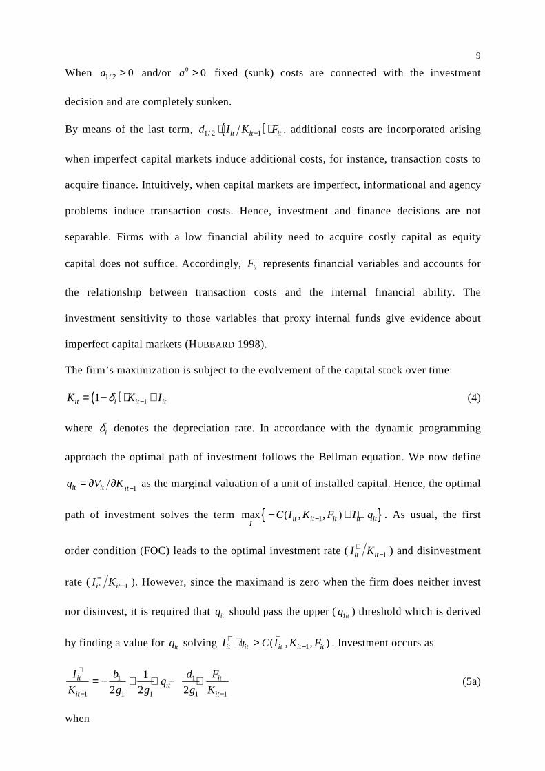
When 1/ 2 0a > and/or 0 0a > fixed (sunk) costs are connected with the investment
decision and are completely sunken.
By means of the last term, ( )1/ 2 1it it itd I K F−⋅ ⋅ , additional costs are incorporated arising
when imperfect capital markets induce additional costs, for instance, transaction costs to
acquire finance. Intuitively, when capital markets are imperfect, informational and agency
problems induce transaction costs. Hence, investment and finance decisions are not
separable. Firms with a low financial ability need to acquire costly capital as equity
capital does not suffice. Accordingly, itF represents financial variables and accounts for
the relationship between transaction costs and the internal financial ability. The
investment sensitivity to those variables that proxy internal funds give evidence about
imperfect capital markets (HUBBARD 1998).
The firm’s maximization is subject to the evolvement of the capital stock over time:
( ) 11it i it itK K Iδ −= − ⋅ + (4)
where iδ denotes the depreciation rate. In accordance with the dynamic programming
approach the optimal path of investment follows the Bellman equation. We now define
1it it itq V K −= ∂ ∂ as the marginal valuation of a unit of installed capital. Hence, the optimal
path of investment solves the term { }1max ( , , )it it it it itI
C I K F I q−− + ⋅ . As usual, the first
order condition (FOC) leads to the optimal investment rate ( 1it itI K+− ) and disinvestment
rate ( 1it itI K−− ). However, since the maximand is zero when the firm does neither invest
nor disinvest, it is required that itq should pass the upper (1itq ) threshold which is derived
by finding a value for itq solving 1( , , )it it it it itI q C I K F+ +−⋅ > . Investment occurs as
1 1
1 1 1 1 1
1
2 2 2it it
itit it
I Fb dq
K g g g K
+
− −= − + ⋅ − ⋅ (5a)
when
10
01
1 1 1 1 11 1
2 itit it
it it
Fa gq q b a g d
K K− −
⋅> = + ⋅ + ⋅ + ⋅ (5b)
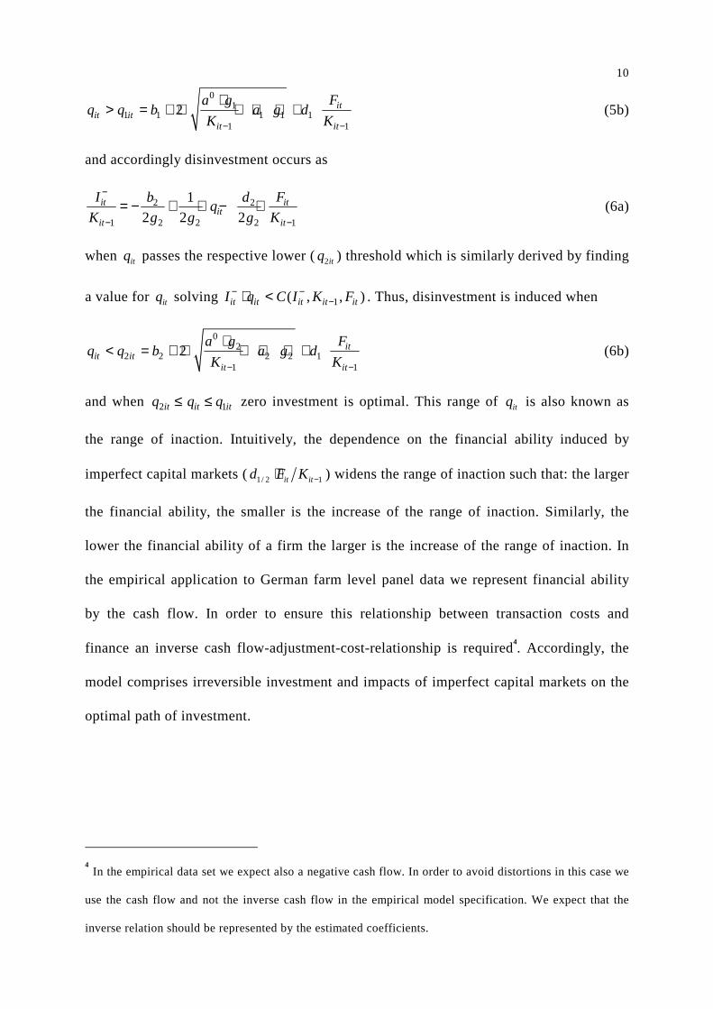
and accordingly disinvestment occurs as
2 2
1 2 2 2 1
1
2 2 2it it
itit it
I Fb dq
K g g g K
−
− −= − + ⋅ − ⋅ (6a)
when itq passes the respective lower (2itq ) threshold which is similarly derived by finding
a value for itq solving 1( , , )it it it it itI q C I K F− −−⋅ < . Thus, disinvestment is induced when
02
2 2 2 2 11 1
2 itit it
it it
Fa gq q b a g d
K K− −
⋅< = + ⋅ + ⋅ + ⋅ (6b)
and when 2 1 it it itq q q≤ ≤ zero investment is optimal. This range of itq is also known as
the range of inaction. Intuitively, the dependence on the financial ability induced by
imperfect capital markets (1/ 2 1it itd F K −⋅ ) widens the range of inaction such that: the larger
the financial ability, the smaller is the increase of the range of inaction. Similarly, the
lower the financial ability of a firm the larger is the increase of the range of inaction. In
the empirical application to German farm level panel data we represent financial ability
by the cash flow. In order to ensure this relationship between transaction costs and
finance an inverse cash flow-adjustment-cost-relationship is required4. Accordingly, the
model comprises irreversible investment and impacts of imperfect capital markets on the
optimal path of investment.
4 In the empirical data set we expect also a negative cash flow. In order to avoid distortions in this case we
use the cash flow and not the inverse cash flow in the empirical model specification. We expect that the
inverse relation should be represented by the estimated coefficients.

11
In all cases, itq refers to the shadow value of capital defined as the discounted future
expectations of the marginal productivity of a unit of installed capital. ABEL and EBERLY
(1994) provide:
{ } ( )2
0 0.5 ( 1)
Xi iX r s it
it t it si i X X i
h Xq h E X e ds
r
ηδη
δ η η σ
∞− + ⋅
+⋅= ⋅ ⋅ =
+ − ⋅ ⋅ − ⋅∫ (7)
According to (7), itq is proportional to the average capital productivity measured by
market data. The important feature of this specification is the incorporation of the
variance ( 2iσ ) of the stochastic part of the demand function accounting for uncertain
future revenues. By means of this specification uncertainty directly affects itq . It follows
that an increase in iσ increases itq . As investments and itq are positively related an
increasing volatility rises investment. However, if the initial value of itq is in the range of
inaction, a small increase in iσ does not induce an investment or disinvestment (ABEL
and EBERLY 1993)5.
Econometric Model
We use farm level panel data which do not contain any market information to construct
itq as defined above. However, an average-type proxy variable would even be
inappropriate in this context. In order to make the model estimable itq is approximated in
terms of observable variables:
'it it itq Zβ ε= + (8)
where β is a parameter vector to be estimated and itZ is the information set for itq
containing variables which proxy the information about the shadow value of capital. For
the first set of variables, in line with NILSEN, SALVANES and SCHIANTARELLI (2007), it is
5 For a further discussion see ABEL et al. (1996).
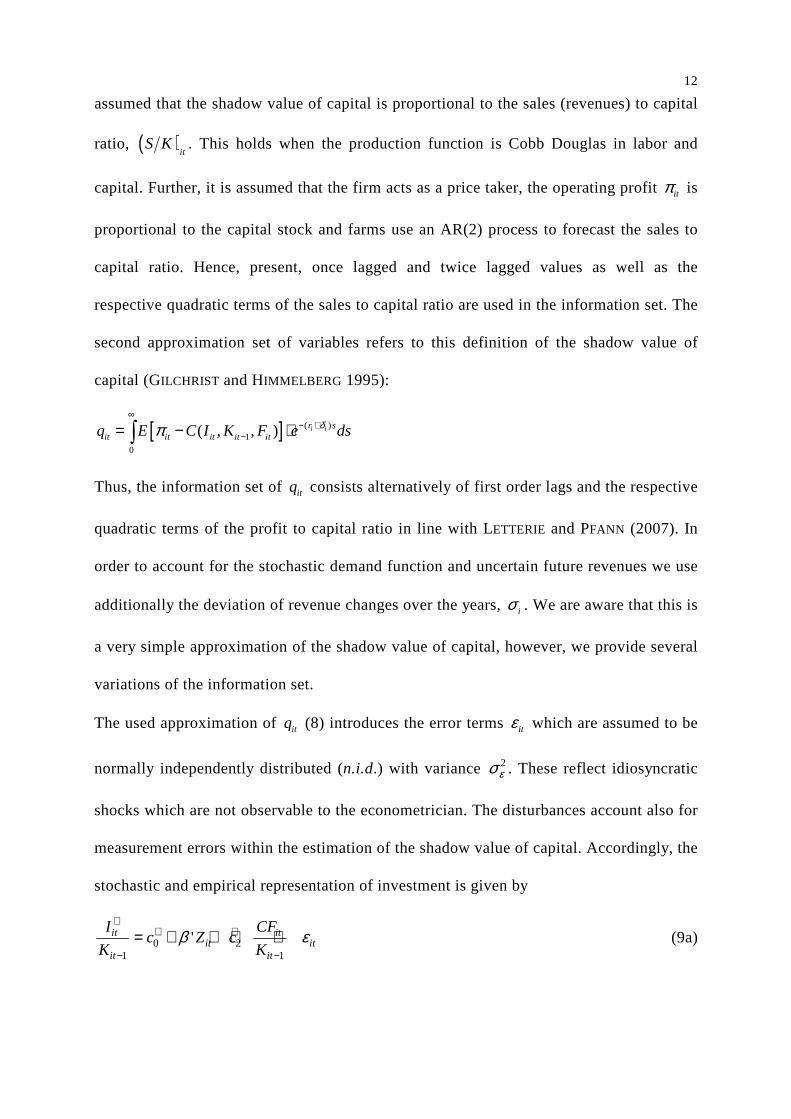
12
assumed that the shadow value of capital is proportional to the sales (revenues) to capital
ratio, ( )it
S K . This holds when the production function is Cobb Douglas in labor and
capital. Further, it is assumed that the firm acts as a price taker, the operating profit itπ is
proportional to the capital stock and farms use an AR(2) process to forecast the sales to
capital ratio. Hence, present, once lagged and twice lagged values as well as the
respective quadratic terms of the sales to capital ratio are used in the information set. The
second approximation set of variables refers to this definition of the shadow value of
capital (GILCHRIST and HIMMELBERG 1995):
[ ] ( )1
0
( , , ) i ir sit it it it itq E C I K F e dsδπ
∞− +
−= − ⋅∫
Thus, the information set of itq consists alternatively of first order lags and the respective
quadratic terms of the profit to capital ratio in line with LETTERIE and PFANN (2007). In
order to account for the stochastic demand function and uncertain future revenues we use
additionally the deviation of revenue changes over the years, iσ . We are aware that this is
a very simple approximation of the shadow value of capital, however, we provide several
variations of the information set.
The used approximation of itq (8) introduces the error terms itε which are assumed to be
normally independently distributed (n.i.d.) with variance 2εσ . These reflect idiosyncratic
shocks which are not observable to the econometrician. The disturbances account also for
measurement errors within the estimation of the shadow value of capital. Accordingly, the
stochastic and empirical representation of investment is given by
0 21 1
'it itit it
it it
I CFc Z c
K Kβ ε
++ +
− −= + + ⋅ + (9a)

13
when6
0 1 21 1
1' 0it
it itit it
CFZ
K Kγ γ β γ ε+ + +
− −+ ⋅ + + ⋅ + > (9b)
and disinvestment is described by
0 21 1
'it itit it
it it
I CFc Z c
K Kβ ε
−− −
− −= + + ⋅ + (10a)
when
0 1 21 1
1' 0it
it itit it
CFZ
K Kγ γ β γ ε− − −
− −+ + + ⋅ + < (10b)
where itCF denotes the cash flow of farm i at time t.
Estimation
This model has the structure of a generalized two-sided tobit model (DIIORIO and FACHIN
2006 refer to a double censored tobit model). The parameter estimates can be obtained by
either maximum likelihood estimation of the full model or alternatively by a two-stage
method. For convenience we use the two-stage Heckman procedure (HECKMAN 1976,
1979; CAMERON and TRIVEDI 2005). In the first step, we estimate a generalized ordered
probit model (BOES and WINKELMANN 2006) to derive the probabilities of investment,
disinvestment and inaction. Using these results of the first stage we obtain the shadow
value of capital itq . In addition, the results from the first step are used to estimate the
necessary selectivity regressors. These are required in the second stage to account for the
sample selection bias induced by the selection equations (9b) and (10b). These regressors
are also known as inverse Mill’s ratios. In the second step, the (dis)investment functions
((9a) and (10a)) are estimated using the Mill’s ratios as additional explanatory variables.
6 In order to make the model estimable the thresholds
1q and
2q are linearly approximated:
0
1 1 1 1 1 0 1 12 1
it itb a g K a g Kγ γ+ +
− −+ ⋅ ⋅ + ⋅ ≅ + ⋅ and 0
2 2 1 2 2 0 1 12 1
it itb a g K a g Kγ γ− −
− −− ⋅ ⋅ + ⋅ ≅ + ⋅ .

14
This ensures that the parameter estimates of the investment and disinvestment functions
are unbiased and consistent (MADDALA 1983).
For the generalized ordered probit model the dummy variable DitI is defined indicating
whether a firm invests ( 1DitI = ), disinvests ( 1D
itI = − ) or is inactive ( 0DitI = ). The inverse
capital stock, 11 itK − , enters the model only through the selection equations (9b) and (10
b) and gives therefore an useful exclusion restriction to identify the model (CAMERON and
TRIVEDI 2005). The generalized ordered probit model can be written as:
10 1 1 2 1
1
10 1 1 2 1
1
1 10 1 1 2 1 0 1 1
log
' /log 1
' /log
' / 'log
Dit
Dit
it it it it
I
it it it it
I
it it it it it it
L
K Z CF K
K Z CF K
K Z CF K K Z
ε
ε
ε
γ γ β γσ
γ γ β γσ
γ γ β γ γ γ βσ
+ + − +− −
=
− − − −− −
=−
+ + − + − − −− − −
=
+ ⋅ − + ⋅− Φ +
+ ⋅ − + ⋅Φ +
+ ⋅ − + ⋅ + ⋅ − +Φ − Φ
∑
∑
2 1
0
/Dit
it it
I
CF K
ε
γσ
−−
=
⋅
∑
(11)
where ( )Φ ⋅ denotes the standard normal cumulative distribution function. The parameters
can only be identified up to a scale parameter and are normalized by εσ which will be
denoted by ∼.
For the second step it is necessary to define the inverse Mill’s ratios for the
(dis)investment equations, itλ+ and itλ− , respectively. These account for the non-linear
selection and are defined as the expected value of itε conditional on being in the
investment or disinvestment regime
( )( )
10 1 1 2 1
10 1 1 2 1
' /
1 ' /
it it it it
it
it it it it
K Z CF K
K Z CF K
φ γ γ β γλ
γ γ β γ
+ + − +− −+
+ + − +− −
+ ⋅ − + ⋅=
− Φ + ⋅ − + ⋅
%% % %
%% % % (12a)
( )( )
10 1 1 2 1
10 1 1 2 1
' /
' /
it it it it
it
it it it it
K Z CF K
K Z CF K
φ γ γ β γλ
γ γ β γ
− − − −− −−
− − − −− −
+ ⋅ − + ⋅=
Φ + ⋅ − + ⋅
%% % %
%% % % (12b)

15
where ( )φ ⋅ denotes the standard normal density function. Accordingly, the resulting
equations for the second stage are defined as follows.
( )0 1 21 1
ˆ'it itit it it
it it
I CFc c Z c u
K Kβ λ
++ + + + +
− −= + ⋅ − + ⋅ +% (13a)
( )0 1 21 1
ˆ'it itit it it
it it
I CFc c Z c u
K Kβ λ
−− − − − −
− −= + ⋅ + + ⋅ +% (13b)
where itu+ and itu− are zero mean error terms. The parameters are defined as 0 1 12c b γ+ = − ,
0 2 22c b γ− = − , 2 1 12c d γ+ = − , 2 2 22c d γ− = − ((5a) and (6a)). The Mills ratios (itλ+ and itλ− )
are multiplied by the parameters 1c+ or 1c
− , respectively, as the error terms enter the
equation through the proxy variable for itq (NILSEN, SALVANES and SCHIANTARELLI
2007). It is assumed that itZ are uncorrelated with the errors itu+ , itu− and itε to ensure that
the generalized ordered probit model yields consistent estimates and standard errors of
the parameters. As there is only one single generated regressor for each equation the
asymptotic t-statistics can be used for inference and the estimators are consistent (PAGAN
1984).
In order to demonstrate the advantages of our approach a simpler linear benchmark model
is defined. The model represents that kind of model which is often used in the analysis of
empirical investment behavior as described in BOND and VAN REENEN (2003) or ADDA
and COOPER (2003).
( )0 1 21 1
'b
it itit it
it it
I CFZ u
K Kα α β α
− −
= + ⋅ + ⋅ +
% (14)
where the superscript b denotes the benchmark model. The disturbances itu are assumed
to be identically independently distributed (i.i.d). A significant cash flow parameter
indicates the dependence of finance and therefore imperfect capital markets. However,
this kind of model does not account for any costly reversibility and ignores furthermore

16
the bias in the linear estimation without selectivity regressors. By means of this model the
ambition is to find out how simpler linear models behave in comparison to the
generalized tobit model with respect to the cash flow sensitivity. The ambition is to show
that the 2-sided tobit model is the appropriate specification when explaining investment
behavior. It is expected that the parameter estimates of the benchmark model differ
significantly from those given by the second stage regressions.
Data and Descriptive Statistics
We use farm level panel data from the national German farm accountancy data network
(FADN) covering the years from 1996 to 2006 (from here: BMELV Testbetriebsnetz).
This dataset is based on annual balance sheet data from representative farms in Germany
and must conform to consistent accounting procedures given by the European
Commission (EU COMMISSION 1989). Specialists in horticulture, orchards, fishery and
forestry are excluded as those have a different capital structure and are difficult to
compare with specialists in agriculture. In the estimation only farms with at least four
consecutive years are considered to ensure consistency, particularly in the estimation of
iσ , the measure of uncertainty. Outliers are imposed by removing farms from the data
sample that are below the 1 % percentile and above the 99 % percentile of the
(dis)investment capital ratio and the sales to capital ratio. These rules are common in
investment literature (BENJAMIN and PHIMISTER 2002; GILCHRIST and HIMMELBERG
1998). Accordingly, the used data set is unbalanced and contains roughly 12 500 farms
(approximately 2 100 in the East and 10 400 in the West) with 6.9 years on average7.
7 It has to be acknowledged that the sample is not fully representative as we do not use any aggregation
factors.
17
35 % of the observations in the West are zero investments and 23 % are investments
whereas in the East 17 % are zero investments and 36 % investments. This indicates for
East and West unequal proportions and the largest share of observations belongs to the
disinvestment regime. Information on annual investments are presented in table 1. For
each year available in the data set the mean investment rate of Germany, East and West
Germany is given.
Table 1. Annual Investment Rates for Germany
mean no. of mean number of mean no. ofinvestment rate observations investment rate observations investment rate observations
1996 0.10 2 520 0.08 1 954 0.16 566
1997 0.10 2 712 0.09 2 148 0.14 564
1998 0.10 2 827 0.09 2 278 0.15 549
1999 0.11 2 269 0.10 1 708 0.14 561
2000 0.10 2 558 0.09 2 024 0.13 534
2001 0.09 2 721 0.09 2 139 0.11 582
2002 0.11 2 228 0.10 1 680 0.14 548
2003 0.11 2 170 0.11 1 605 0.13 565
2004 0.11 1 879 0.11 1 428 0.13 451
2005 0.11 2 041 0.10 1 492 0.12 549
2006 0.10 1 949 0.09 1 425 0.13 524
Note: The database is the BMELV Testbetriebsnetz 1996-2006.
Germany West Germany East Germany
year
The aggregated investment rates are rather constant over time. However, in the Eastern
federal states a higher variation and higher average investment rates are observable. This
might be a first indication for necessary modernization investments in the transition
period. However, it needs to be acknowledged that the used capital stock in Eastern farms
might be under-evaluated since it was installed before 1990.
The data confirm the unequal capital structure at the farm level in East and West
Germany. The average equity ratio amounts to 56 % and 82 % of total capital stock,
respectively. This rather high equity ratio in the West indicates financial strength of the
farms which might additionally be a signal for a lower dependence on finance. In equal
measure it can be shown that the average debt capital ratio (due to missing values in the
data set only bank loans are considered) is only 17 % in the West whereas bank loans in
18
the East are more important with a share by about 33 %. This comparably high share in
the East signals a stronger dependency on the access to capital.
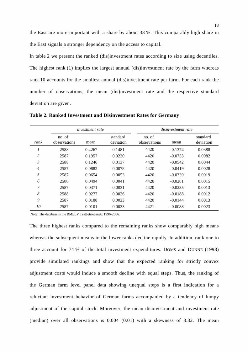
In table 2 we present the ranked (dis)investment rates according to size using decentiles.
The highest rank (1) implies the largest annual (dis)investment rate by the farm whereas
rank 10 accounts for the smallest annual (dis)investment rate per farm. For each rank the
number of observations, the mean (dis)investment rate and the respective standard
deviation are given.
Table 2. Ranked Investment and Disinvestment Rates for Germany
no. of standard no. of standard rank observations mean deviation observations mean deviation
1 2588 0.4267 0.1481 4420 -0.1374 0.0388
2 2587 0.1957 0.0230 4420 -0.0753 0.0082
3 2588 0.1246 0.0137 4420 -0.0542 0.0044
4 2587 0.0882 0.0078 4420 -0.0419 0.0028
5 2587 0.0654 0.0053 4420 -0.0339 0.0019
6 2588 0.0494 0.0041 4420 -0.0281 0.0015
7 2587 0.0371 0.0031 4420 -0.0235 0.0013
8 2588 0.0277 0.0026 4420 -0.0188 0.0012
9 2587 0.0188 0.0023 4420 -0.0144 0.0013
10 2587 0.0101 0.0033 4421 -0.0088 0.0023
Note: The database is the BMELV Testbetriebsnetz 1996-2006.
disinvestment rateinvestment rate
The three highest ranks compared to the remaining ranks show comparably high means
whereas the subsequent means in the lower ranks decline rapidly. In addition, rank one to
three account for 74 % of the total investment expenditures. DOMS and DUNNE (1998)
provide simulated rankings and show that the expected ranking for strictly convex
adjustment costs would induce a smooth decline with equal steps. Thus, the ranking of
the German farm level panel data showing unequal steps is a first indication for a
reluctant investment behavior of German farms accompanied by a tendency of lumpy
adjustment of the capital stock. Moreover, the mean disinvestment and investment rate
(median) over all observations is 0.004 (0.01) with a skewness of 3.32. The mean
19
(median) investment rate is 0.10 (0.05) and the mean (median) disinvestment rate is -0.04
(-0.03). These findings indicate asymmetries in the adjustment of the capital stock.
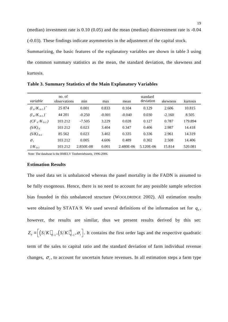
Summarizing, the basic features of the explanatory variables are shown in table 3 using
the common summary statistics as the mean, the standard deviation, the skewness and
kurtosis.
Table 3. Summary Statistics of the Main Explanatory Variables
no. of standard variable observations min max mean deviation skewness kurtosis
(I it /K it-1 ) + 25 874 0.001 0.833 0.104 0.129 2.606 10.815
(I it /K it-1 ) - 44 201 -0.250 -0.001 -0.040 0.030 -2.160 8.505
(CF it /K it-1 ) 103 212 -7.505 3.229 0.028 0.127 0.787 179.894
(S/K)it 103 212 0.023 3.404 0.347 0.406 2.987 14.418
(S/K)it-1 85 562 0.023 3.402 0.335 0.336 2.961 14.319
σ i 103 212 0.005 4.606 0.489 0.302 2.508 14.406
1/K it-1 103 212 2.850E-08 0.001 2.480E-06 5.120E-06 15.814 520.081
Note: The database is the BMELV Testbetriebsnetz, 1996-2006.
Estimation Results
The used data set is unbalanced whereas the panel mortality in the FADN is assumed to
be fully exogenous. Hence, there is no need to account for any possible sample selection
bias founded in this unbalanced structure (WOOLDRIDGE 2002). All estimation results
were obtained by STATA 9. We used several definitions of the information set for itq ,
however, the results are similar, thus we present results derived by this set:
( ) ( )2
1 1, ,it iit it
Z S K S K σ− −
=
. It contains the first order lags and the respective quadratic
term of the sales to capital ratio and the standard deviation of farm individual revenue
changes, iσ , to account for uncertain future revenues. In all estimation steps a farm type
20
dummy itDT8 and a size dummy itDS
9 are used to reduce possible effects which could bias
the constant terms. Further, farm individual averages of all explanatory variables are
included to account for possible heterogeneity between the farms10.
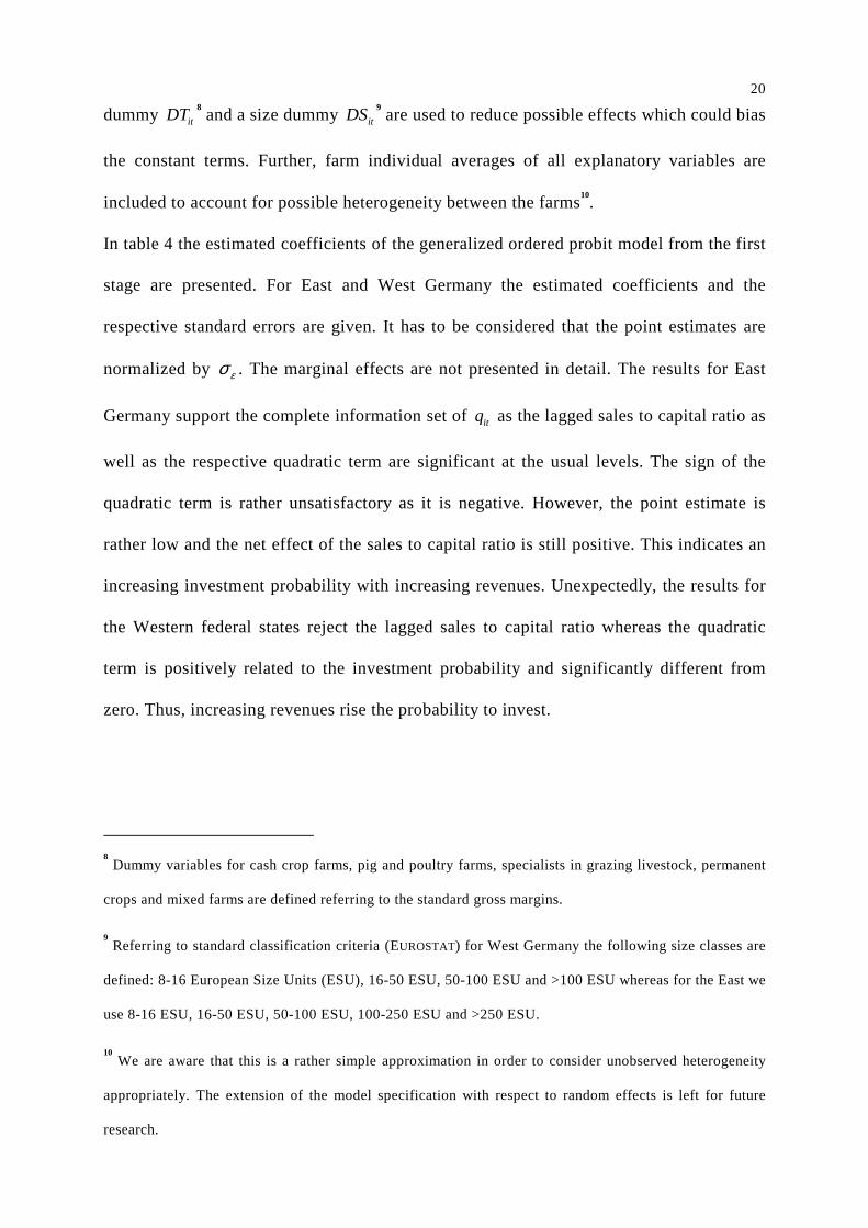
In table 4 the estimated coefficients of the generalized ordered probit model from the first
stage are presented. For East and West Germany the estimated coefficients and the
respective standard errors are given. It has to be considered that the point estimates are
normalized by εσ . The marginal effects are not presented in detail. The results for East
Germany support the complete information set of itq as the lagged sales to capital ratio as
well as the respective quadratic term are significant at the usual levels. The sign of the
quadratic term is rather unsatisfactory as it is negative. However, the point estimate is
rather low and the net effect of the sales to capital ratio is still positive. This indicates an
increasing investment probability with increasing revenues. Unexpectedly, the results for
the Western federal states reject the lagged sales to capital ratio whereas the quadratic
term is positively related to the investment probability and significantly different from
zero. Thus, increasing revenues rise the probability to invest.
8 Dummy variables for cash crop farms, pig and poultry farms, specialists in grazing livestock, permanent
crops and mixed farms are defined referring to the standard gross margins.
9 Referring to standard classification criteria (EUROSTAT) for West Germany the following size classes are
defined: 8-16 European Size Units (ESU), 16-50 ESU, 50-100 ESU and >100 ESU whereas for the East we
use 8-16 ESU, 16-50 ESU, 50-100 ESU, 100-250 ESU and >250 ESU.
10 We are aware that this is a rather simple approximation in order to consider unobserved heterogeneity
appropriately. The extension of the model specification with respect to random effects is left for future
research.
21
The findings affirm uncertainty belonging to the information set for itq . At first glance
the differing signs of the parameter estimates for iσ between East and West Germany are
surprising. Thereby, only the parameter estimates for East Germany are consistent with
the theoretical model. The marginal effects for East and West are rather small but also
differ by sign. An increase in uncertainty increases the probability to invest (+0.04) and
induces a declining probability to disinvest (-0.05). On the contrary, the estimates for
West Germany indicate that an increase in uncertainty induces a decline in the probability
to invest (-0.03) but increases probability to disinvest (+0.03).
Table 4. Results from the First Stage Generalized Ordered Probit Model
Proxy variables for q
(S/K)it-1
((S/K)it-1 ) 2
σ i
Variables of the investment and disinvestment thresholds q1 and q2
q 1 q 2 q 1 q 2
CF it /K it-1 0.963 0.906 0.404 0.835[0.094]** [0.095]** [0.063]** [0.072]**
1/K it-1 -50 584 103 491 -22 361 120 907[10 521]** [10 205]** [2 933]** [3 604]**
Constant 0.011 -0.066 -1.153 0.242[0.100] [0.100] [0.094]** [0.076]**
Log-Likelihood
Note: Standard errors are in brackets. Single (*) and double (**) asterisks denote significant at 5 % and 1 %, respectively.
-69 447-11 907
[0.066]
0.147[0.027]**
-0.062
[0.069]**
0.125[0.036]**
[0.173]**
-0.444
0.051
[0.016]**
West GermanyEast Germany
1.924
The range of inaction depends on the constant, the inverse capital stock and the cash
flow. If irreversibility is present, the parameter estimates for the constant terms and the
inverse capital stock need to be significant with differing point estimates by investment
and disinvestment probability. To induce optimal inactivity, the resulting investment
threshold 1itq exceeds the disinvestment threshold 2itq . The cash flow coefficient
22
indicates additional transaction costs to acquire finance for investments and is expected to
be significant if agency problems or informational asymmetries characterize the capital
market. Imperfect capital markets should increase the range of inaction but an increasing
financial ability should reduce the respective investment threshold.
In the West, the point estimates of the constant, the inverse capital stock and the cash
flow parameter differ significantly by the investment and disinvestment threshold which
is confirmed by the Wald-test rejecting the null of equal parameters. The respective
thresholds for West Germany are:
1 1 1ˆ ˆ 1.153 22230 0.404it it it it itq q K CF K− −> = + − ⋅ (15a)
2 1 1ˆ ˆ 0.242 120970 0.835it it it it itq q K CF K− −< = − − − ⋅ (15b)
Using the means of the respective variables the upper threshold is on average 1.17 and the
respective lower threshold is about -0.47. Interestingly, the thresholds might be negative
inducing that even losses or in other words a negative capital productivity is possible
without inducing a disinvestment.
In the East, the constant term is rejected for the investment and disinvestment threshold.
This implies that the range of inaction is mainly determined by the inverse capital stock,
i.e. the size of the farm, and the cash flow. The parameter estimates for the capital stock
differ significantly by investment and disinvestment threshold indicating a range of
inactivity induced by costly reversibility. The parameter estimates for the cash flow do
not significantly differ; the respective Wald-test cannot reject the null of equal estimates
for the investment and disinvestment threshold. Accordingly, additional transaction costs
due to capital market imperfections affect the investment and disinvestment decision at
the same level.
The cash flow sensitivity is of particular interest as it reflects imperfect capital markets.
The results confirm weaker capital markets and a stronger dependence on finance for East
23
Germany. The cash flow sensitivity of the investment trigger (0.96) exceeds the
respective estimate for the West (0.40). This difference in the cash flow sensitivity
between East and West Germany is even more pronounced when only co-operatives,
stock companies and corporate farms as the main legal form of the former state owned co-
operatives are considered (+2.66). Interestingly, the cash flow parameters show nearly no
difference between East and West Germany with regard to the impact on the
disinvestment probability. It seems that liquidity has the same importance in the
disinvestment decision regardless of the capital market conditions. In the Western federal
states, the effect of finance on the investment decision is less pronounced than on the
disinvestment decision. The marginal effects for the Western federal states affirm a
positive relation of the cash flow and the probability to invest (+0.09) whereas the
relation is negative for the disinvestment threshold (-0.29). In the East, the effects have
the same direction as in the West but are more pronounced (+0.35 and -0.36).
It can be shown that irreversibility, uncertainty and the dependence of finance coexist and
affect investment decisions of farms. Under weaker conditions in the capital market the
availability of finance is more important confirmed by the higher cash flow sensitivity in
East Germany. In table 5 the results of the second stage regression explaining the
(dis)investment rates and the results of the rather simple benchmark model (14) are given.
The estimates confirm a positive and significant relation of the derived shadow value of
capital to the investment and disinvestment rates. However, the point estimates are rather
low. These findings are consistent with the theoretical model and give evidence on the
quadratic term of the adjustment cost function. The point estimates in East and West for
the disinvestment equation are higher than the point estimates for the investment equation
indicating asymmetric adjustments.
24
Table 5. Results from the Second Stage Regressions
Variable (I it /K it-1 ) + (I it /K it-1 ) - (I it /K it-1 ) b (I it /K it-1 ) + (I it /K it-1 ) - (I it /K it-1 ) b
q it 0.048 0.143 0.16 0.027 0.203 0.264[0.014]** [0.006]** [0.009]** [0.008]** [0.002]** [0.007 ]**
CF it /K it-1 0.106 0.072 0.133 0.211 0.071 0.137[0.014]** [0.006]** [0.009]** [0.008]** [0.003]** [0.005 ]**
Constant 0.141 -0.193 0.017 0.109 -0.179 -0.007[0.015]** [0.007]** [0.010] [0.021]** [0.003]** [0.008]
Observations 4 352 6 385 10 737 15 333 28 899 44 232
Note: Standard errors are in brackets. Single (*) and double (**) asterisks denote significant at 5 % and 1 %, respectively.
East Germany West Germany
The constant term is not rejected at the 1 % significance level attesting the linear term of
the adjustment cost function. The unequal point estimates suggest costly reversibility. The
constant term is expected to be negative, which is only confirmed by the disinvestment
equations. Interestingly, the cash flow sensitivity is rather low for the East and West. The
investment cash flow relation is positive and at first glance, this relation seems different
compared to the financial parameter in the theoretical model. As mentioned above, an
inverse relationship between the cash flow and investment is required. An increase in the
inverse cash flow would induce increasing investment rates even though the sign of the
inverse cash flow in the investment equation is negative. This reduction of the investment
rate arises from the additional transaction costs in imperfect capital markets but declines
as financial ability increases.
The results of the simpler benchmark model, ( )1
b
it itI K − , which does not account for any
selectivity bias and ignores the range of inaction, show that the parameter estimates differ
in comparison to the results of the second stage regressions. The constant term is rejected
in the simple model and the quadratic term of the adjustment cost function is given a
higher weight compared to the second stage regressions. Ambiguously, the impact of the
cash flow on investment, i.e. the cash flow sensitivity, is overestimated in the East and
underestimated in the West. At first glance there is no statement possible which model
25
should be preferred. Therefore, the Chow-test, based on the F-test, is applied in order to
test if the parameter estimates differ leading to a separate estimation of the investment
and disinvestment equations (DAVIDSON and MACK INNON 2004). The Chow-test rejects
the null of equal parameters at 1 %. This confirms the differences – founded in a more
sophisticated theoretical basis – and indirectly, the need to account for the range of
inaction.
Conclusions
The aim of this study has been to explain empirically observed phenomena as frequent
periods of zero investments, high investment reluctance and in transition economies,
rather low investment rates despite the need of rationalization and modernization
investments. More precisely, the intention has been to show that imperfect capital
markets, irreversibility and uncertainty coexist and jointly affect investment behavior of
farms. Imperfect capital markets released by agency problems induce additional
transaction costs to acquire finance or even a limited access to capital. However, impacts
of agency problems and informational asymmetries in the capital market cannot solely
explain investment reluctance. Costly reversibility and uncertain future expectations lead
to retention and a range of inactivity along the optimal path of investment. Therefore, we
have defined a stochastic and dynamic investment model which explicitly accounts for
consequences of capital market imperfections inducing the dependence on finance and for
coexistent irreversibility and uncertain future revenues. This is achieved by an augmented
adjustment cost function as the presence of irreversibility does not allow to use strictly
convex adjustment costs as traditional q-theory proposes. This augmented cost function
accounts for sunk costs, costly reversibility and transaction costs to acquire finance. The
econometric model is consistent with the theoretical model and has the structure of a two-
sided generalized tobit model. The application of this model to German farm level panel

26
data delivers insights into a transition economy (East Germany) and allows direct
comparisons to an established market economy (West Germany).
The empirical results confirm coexistent capital market frictions, costly reversibility and
uncertainty. The findings support the hypothesis that farms in East Germany face
significantly higher transaction costs expressed in terms of a higher cash flow sensitivity.
Contrasting these findings with results from a simpler linear model, solely accounting for
imperfect capital markets, affirms that a disregard of irreversibility reduces the
informative power of such models.
We conclude that a more general form of models like tobit models are required to account
for both, capital market imperfections as well as sunk costs and the respective range of
inaction. These insights provide a new basis to explain farm growth, development of farm
structure and thus structural change. Beyond the scientific guess of this paper the results
imply that farmers’ reluctance to invest is a result of dynamically optimal behavior when
capital markets are perfect. Hence, a slow capacity adjustment per se does not justify
policy intervention. When additionally capital markets are imperfect, retention of capacity
adjustments increases as access to capital is limited. If there is evidence on imperfect
capital markets, policy intervention should also focus on the reduction of the degree of
imperfection to facilitate finance. The design of support schemes, for instance investment
subsidies or retirement programs in the context of payments from the European Union,
should take these findings into account.
Nonetheless, we are aware that the empirical model specification has potential for
improvement. Main point for future research is the consideration of unobserved
heterogeneity within the estimation. Another important issue refers to the comparison of
the complex tobit model with the simpler linear model. After we have shown the limited
validity of such models, we further aim to quantify the direction of the expected bias
27
within empirical applications disregarding the range of inaction and to find out how this
bias limits conclusions drawn from such findings.
References
ABEL, A., DIXIT , A., EBERLY, J., PINDYCK, R. (1996): Options, the Value of Capital, and
Investment. The Quarterly Journal of Economics 111(3):753-777.
ABEL, A., EBERLY, J. (1993): A Unified Model of Investment under Uncertainty. Working
Paper No. 4296 National Bureau of Economic Research (NBER).
ABEL, A., EBERLY, J. (1994): A Unified Model of Investment under Uncertainty. The
American Economic Review 84(5): 1369-1384.
ABEL, A., EBERLY, J. (2002): Investment and q with Fixed Costs. An Empirical Analysis.
Kellogg School of Management Northwestern University Working Paper 2002.
ADDA, J., COOPER, R. (2003): Dynamic Economics. Quantitative Methods and Applications.
The MIT Press Cambridge (MA).
BAHRS, E., FUHRMANN, R., MUZIOL, O. (2004): Die künftige Finanzierung landwirtschaftlicher
Betriebe. Finanzierungsformen und Anpassungsstrategien zur Optimierung der
Finanzierung. Landwirtschaftliche Rentenbank (Hrsg.): Herausforderungen für die
Agrarfinanzierung im Strukturwandel – Ansätze für Landwirte, Banken, Berater und
Politik. Schriftenreihe Bd. 19: 203-247.
BARRY, P., BIERLEN, R., SOTOMAYOR, N. (2000): Financial Structure of Farm Businesses
Under Imperfect Capital Markets. In: American Journal of Agricultural Economics 82(4):
920-933.
BENJAMIN, C., PHIMISTER, E. (2002): Does Capital Market Structure Affect Farm Investment?
American Journal of Agricultural Economics 84(4): 1115-1129.
BLISSE, H., HANISCH, M., HIRSCHAUER, N., KRAMER, J., ODENING, M. (2004): Risikoorientierte
Agrarkreditvergabe – Entwicklung und Konsequenzen. Landw. Rentenbank (Hrsg.):
28
Herausforderungen für die Agrarfinanzierung im Strukturwandel – Ansätze für Landwirte,
Banken, Berater und Politik. Schriftenreihe Bd. 19: 203-247.
BOES, S., WINKELMANN R. (2006): Ordered Response Models. Allgemeines Statistisches
Archiv 90(1): 165-180.
BÖHM, H., FUNKE, M., SIGFRIED, N. (1999): Discovering the Link between Uncertainty and
Investment. Microeconometric Evidence from Germany. Selected paper presented at the
HWWA Workshop on “Uncertainty and Factor Demands”, Hamburg, August 26-27.
BOND, S., MEGHIR, C. (1994): Dynamic Investment Models and the Firm’s Financial Policy.
In: Review of Economic Studies 61(2): 197-222.
BOND, S., VAN REENEN, J. (2003): Microeconometric Models of Investment and
Employment. The Institute for Fiscal Studies, Mimeo 2003.
CABALLERO, R. (1997): Aggregate Investment. Working Paper 6264 National Bureau of
Economic Research (NBER).
CAMERON, A., TRIVEDI, P. (2005): Microeconometrics. Methods and Applications. Cambridge
University Press, New York.
CHIRINKO, R. (1993): Business Fixed Investment Spending: Modelling Strategies, Empirical
Results, and Policy Implications. In: Journal of Economic Literature 31(4): 1875-1911.
COOPER, R., HALTIWANGER, J. (2006): On the Nature of Capital Adjustment Costs. Review of
Economic Studies 73(3): 611-633.
DAVIDSON, R., MACKINNON, J. (2004): Econometric Theory and Methods. Oxford University
Press, New York.
DIIORIO, F., FACHIN, S. (2006): Maximum Likelihood Estimation of Input Demand Models.
Statistical Methods and Applications 15(1): 129-137.
DOMS, M.; DUNNE, T. (1998): Capital Adjustment Patterns in Manufacturing Plants. Review
of Economic Dynamics 1(2): 409-429.

29
DIXIT , A., PINDYCK, R. (1994): Investment under Uncertainty. Princeton University Press,
New Jersey.
EU COMMISSION (1989): Farm Accountancy Data Network: An A-Z of Methodology. Official
Publications of the European Communities, Luxembourg.
GILCHRIST, S., HIMMELBERG, C. (1995): Evidence on the Role Cash Flow for Investment.
Journal of Monetary Economics 36(3): 541-572.
GILCHRIST, S., HIMMELBERG, C. (1998): Investment, Fundamentals and Finance. Working
Paper 6652 National Bureau of Economic Research (NBER).
HAMERMESH, D. (1992): A General Model of Dynamic Labor Demand. The Review of
Economics and Statistics 74(4): 733-37.
HAMERMESH, D., PFANN, G. (1996): Adjustment Cost in Factor Demand. Journal of Economic
Literature 34(3): 1264-1292.
HECKMAN, J. (1976): The Common Structure of Statistical Models of Truncation, Sample
Selection, and Limited Dependent Variables and a Simple Estimator for Such Models.
Annals of Economic and Social Measurement 5(Fall 1976): 475-492.
HECKMAN, J. (1979): Sample Selection Bias as a Specification Error. Econometrica 47(1):
153-161.
HUBBARD, R. (1998): Capital-Market Imperfections and Investment. Journal of Economic
Literature 36(1): 193-225.
LENSINK, R., BO, H. (2001): Investment, Capital Market Imperfections, and Uncertainty.
Theory and Empirical Results. University of Groningen, The Netherlands.
LETTERIE, W., PFANN, G. (2007): Structural Identification of High and Low Investment
Regimes. Journal of Monetary Economics, forthcoming.
MADDALA , G. (1983): Limited-Dependent and Qualitative Variables in Econometrics.
Econometric Society Monographs, Cambridge University Press, Cambridge.
30
NILSEN, O., SCHIANTARELLI , F. (2003): Zeros and Lumps in Investment: Empirical Evidence
on Irreversibilities and Non-Convexities. Review of Economics and Statistics 85(4): 1021-
1037.
NILSEN, O., SALVANES, K., SCHIANTARELLI , F. (2007): Employment Changes, the Structure of
Adjustment Costs, and Plant Size. European Economic Review, forthcoming.
PAGAN, A. (1984): Econometric Issues in the Analysis of Regressions with Generated
Regressors. International Economic Review 25(1): 221-47.
PAVEL, F.; SHERBAKOV, A.; VERSTYUK, S. (2004): Firms’ Fixed Capital Investment under
Restricted Capital Markets. Institute for Economic Research and Policy consulting (IER)
Working Paper 26, Kiew (Ukraine).
ROTHE, A.; LISSITSA, A. (2005): Der ostdeutsche Agrarsektor im Transformationsprozess –
Ausgangssituation, Entwicklung und Problembereich, IAMO Discussion Paper No. 81,
Halle (Saale).
RIZOV, M. (2004): Firm Investment in Transition: Evidence from Romanian Manufacturing.
Economics of Transition 12(4): 721-746
WOOLDRIDGE, J. (2002): Econometric Analysis of Cross Section and Panel Data. The MIT
Press, Cambridge (MA).


![Irreversibility and the second law of thermodynamicsusers.ntua.gr/rogdemma/Irreversibility and the... · Irreversibility and the second law of ... 1Some authors [14] propose an alternative](https://static.cupdf.com/doc/110x72/5ebc512431aa487d260ac79f/irreversibility-and-the-second-law-of-and-the-irreversibility-and-the-second.jpg)