


Inside Out: Inverse ProblemsMSRI PublicationsVolume 47, 2003
Inverse Acoustic and Electromagnetic
Scattering Theory
DAVID COLTON
Abstract. This paper is a survey of the inverse scattering problem for
time-harmonic acoustic and electromagnetic waves at fixed frequency. We
begin by a discussion of “weak scattering” and Newton-type methods for
solving the inverse scattering problem for acoustic waves, including a brief
discussion of Tikhonov’s method for the numerical solution of ill-posed
problems. We then proceed to prove a uniqueness theorem for the inverse
obstacle problems for acoustic waves and the linear sampling method for
reconstructing the shape of a scattering obstacle from far field data. In-
cluded in our discussion is a description of Kirsch’s factorization method
for solving this problem. We then turn our attention to uniqueness and re-
construction algorithms for determining the support of an inhomogeneous,
anisotropic media from acoustic far field data. Our survey is concluded
by a brief discussion of the inverse scattering problem for time-harmonic
electromagnetic waves.
1. Introduction
The field of inverse scattering, at least for acoustic and electromagnetic waves,
can be viewed as originating with the invention of radar and sonar during the
Second World War. Indeed, as every viewer of World War II movies knows, the
ability to use acoustic and electromagnetic waves to determine the location of
hostile objects through sea water and clouds played a decisive role in the outcome
of that war. Inspired by the success of radar and sonar, the prospect was raised
of the possibility of not only determining the range of an object from the trans-
mitter, but to also image the object and thereby identify it, i.e. to distinguish
between a whale and a submarine or a goose and an airplane. However, it was
soon realized that the problem of identification was considerably more difficult
than that of simply determining the location of a target. In particular, not only
was the identification problem computationally extremely expensive, and indeed
beyond the capabilities of post-war computing facilities, but the problem was
also ill-posed in the sense that the solution did not depend continuously on the
67

68 DAVID COLTON
measured data. It was not until the 1970’s with the development of the math-
ematical theory of ill-posed problems by Tikhonov and his school in the Soviet
Union and Keith Miller and others in the United States, together with the rise of
high speed computing facilities, that the possibility of imaging began to appear
as a realistic possibility. Since that time, the mathematical basis of the acoustic
and electromagnetic inverse scattering problem has reached a level of maturity
that the imaging hopes expressed in the early post-war years have to a certain
extent been realized, at least in the case of electromagnetic waves with the in-
vention of synthetic aperature radar [3], [8]. However, as the imaging demands
have increased so have the mathematical and computational expectations and
hence at this time it seems appropriate to make an attempt at describing the
state of the art in the mathematical foundations of acoustic and electromagnetic
inverse scattering theory. This article is directed towards that goal.
Before proceeding, a few caveats are perhaps in order. The first one is obvious:
we are not proposing to survey the entire field of inverse scattering theory in a
few pages. In particular, we will restrict our attention to a specific area, that
is inverse scattering in the frequency domain and deterministic models. This
means such important topics as time-reversal and scattering by random media
are ignored. Even within this restrictive framework we will be selective and hence
opinionated. In particular, our view is that the mathematical field of inverse
scattering theory should remain close to the applications and in particular should
have the numerical solution of practical imaging problems in “real time” as a high
priority. Uniqueness theorems are important since they indicate what is possible
to image in an ideal noise-free world but not all reconstruction algorithms are
equally valuable from this point of view. Proceeding with such judgments, since
the inverse scattering problem is ill-posed, restoring stability is clearly of central
importance, but again not all stability results are of equal value. In particular,
in order to restore stability some type of a priori information is needed and an
estimate on the noise level is in general more realistic than the knowledge of, for
example, an a priori bound on the curvature of the scattering object. It is freely
acknowledged that points of view other than our own are both reasonable and
legitimate and we are only emphasizing our own view here in order to warn the
reader of what to expect in the pages that follow.
Before proceeding to a discussion of the inverse scattering problem and meth-
ods for its numerical solution we need to be clear on what inverse scattering
problem we are talking about since depending on what a priori information is
available there are many inverse scattering problems! For example, in using ul-
trasound to image the human body it is not unreasonable to assume that the
density is known and equal to the density of water. In this case incident waves at
a single fixed frequency are sufficient for imaging purposes whereas this is not the
case if the density is not known a priori. On the other hand in imaging a target
that has been (partially) coated by an unknown material, it is not reasonable
to assume that the boundary condition on the surface of the scatterer is known.
INVERSE ACOUSTIC AND ELECTROMAGNETIC SCATTERING THEORY 69
Indeed, in my opinion, this last example is more typical in the sense that one
usually knows neither the shape nor the material properties of a scattering ob-
ject and hence neither the shape nor boundary conditions are known. Of course
if a priori information on the material properties of the scatterer are known (as,
for example, in the case of ultrasound imaging of the human body) it is usually
beneficial to use an algorithm which makes use of this information.
The plan of this paper is as follows. Except for the final section, we shall con-
centrate on the scattering of time-harmonic acoustic waves at a fixed frequency.
Hence in Section 2 we shall formulate the acoustic scattering problem and discuss
various inverse scattering problems and their solution by either “weak-scattering”
or Newton-type methods. These two methods are the work horses of inverse scat-
tering and typically lead to the problem of solving linear integral equations of the
first kind arising in either the weak-scattering approximation or in the computa-
tion of the Fréchet derivative of a nonlinear operator. With this as motivation we
shall give a brief introduction to Tikhonov’s method for the numerical solution
of ill-posed problems.
The methods presented in Section 2 for solving acoustic inverse scattering
problems rely on rather strong a priori information on the scattering object. In
Section 3 we shall turn to more recent methods which avoid such strong assump-
tions but at the expense of needing more data. In particular, we shall concentrate
on the case of obstacle scattering and prove the Kirsch–Kress uniqueness theo-
rem [46] which in turn serves as motivation for the linear sampling method for
determining the shape of the scatterer [12],[42]. We shall in addition present a
recent optimization scheme of Kirsch which has certain attractive characteristics
and is closely related to the linear sampling method [44].
In Section 4 we will first consider acoustic inverse scattering problems asso-
ciated with an isotropic inhomogeneous medium and begin with the uniqueness
theorems of Nachman [53], Novikov [57] and Ramm [66]. In this case special
problems occur in the case of scattering in R2. We will again discuss the linear
sampling method for determining the support of the inhomogeneous scatter-
ing object, leading to an investigation of the existence, uniqueness and spectral
properties of the interior transmission problem [13], [14], [19], [67]. We will then
proceed to an extension of these results to the case of anisotropic media. In
contrast to the case of isotropic media, variational methods rather than integral
equation techniques are a more convenient tool in this case [6], [7], [31].
Finally, in Section 5, we consider the inverse scattering problem for Max-
well’s equations and extend some of the results in the previous sections to this
situation. However, much of what is known for the scalar case of acoustic waves
remains unknown in the vector case and hence is a rich area for future study.
To this end, we conclude our survey with a list of open problems for the electro-
magnetic inverse scattering problem.

70 DAVID COLTON
2. The Inverse Scattering Problem for Acoustic Waves
We now consider the scattering of a time harmonic acoustic wave of frequency
ω by an inhomogeneous medium of compact support D having density ρD(x) and
sound speed cD(x), x ∈ D ⊂ R3. We assume that the boundary ∂D is of class
C2 having unit outward normal ν (although much of the analysis which follows
is also valid for Lipschitz domains-see [4],[6]) and that ρD, cD ∈ C2(D). Then
if the host medium is homogeneous with density ρ and sound speed c, the wave
number k is defined by k = ω/c,
n(x) = c/c(x), x ∈ D
and the pressure p(x, t) is given by
p(x, t) =
Re(u(x)e−iωt) if x ∈ R3 \D,
Re(v(x)e−iωt) if x ∈ D,
then u ∈ C2(R3 \ D)⋂
C1(R3 \D) and v ∈ C2(D)⋂
C1(D) satisfy the acoustic
transmission problem
∆u+ k2u = 0 in R3 \ D, (2–1a)
ρD(x)∇(
1
ρD(x)∇v
)
+ k2n(x)v = 0 in D, (2–1b)
u = ui + us, (2–1c)
limr→∞
r(
∂us
∂r− ikus
)
= 0, (2–1d)
u = v
1
ρ
∂u
∂ν=
1
ρD
∂v
∂ν
on ∂D,
on ∂D,(2–1e)
where ui is the incident field, which we assume is given by
ui(x) = eikx·d, |d| = 1,
and the Sommerfeld radiation condition (2–1d) holds uniformly in x = x/|x|,r = |x|.
To allow the possibility of absorption in D we allow n to possibly have a
positive imaginary part; that is, in addition to Ren(x) > 0 for x ∈ D we require
that
Imn(x) ≥ 0
for x ∈ D. The existence of a unique solution to (2–1) has been established by
Werner [73].
For the sake of simplicity, we shall be concerned in this and the next two
sections with certain special cases of the above transmission problem. In par-
ticular, if ρD → ∞ we are led to the exterior Neumann problem for u ∈

INVERSE ACOUSTIC AND ELECTROMAGNETIC SCATTERING THEORY 71
C2(R3 \ D) ∩ C1(R3 \D),
∆u+ k2u = 0 in R3 \ D, (2–2a)
u = ui + us, (2–2b)
limr→∞
r(
∂us
∂r− ikus
)
= 0, (2–2c)
∂u
∂ν= 0 on ∂D; (2–2d)
if ρD → 0 we are led to the exterior Dirichlet problem for u ∈ C2(R3 \ D) ∩C(R3 \D),
∆u+ k2u = 0 in R3 \ D, (2–3a)
u = ui + us, (2–3b)
limr→∞
r(
∂us
∂r− ikus
)
= 0, (2–3c)
u = 0 on ∂D; (2–3d)
and if ρ = ρD we are led to the inhomogeneous medium problem for u ∈C1(R3)
⋂
C2(R3 \ ∂D),
∆u+ k2n(x)u = 0 in R3, (2–4a)
u = ui + us, (2–4b)
limr→∞
r(
∂us
∂r− ikus
)
= 0, (2–4c)
where n(x) = 1 in R3 \ D.
For the purpose of exposition, in the sequel we shall restrict our attention to
the exterior Dirichlet problem and inhomogeneous medium problem (the exterior
Neumann problem can be treated in essentially the same way as the exterior
Dirichlet problem).
We can now be more explicit about what we mean by the acoustic inverse scat-
tering problem. In particular, using Green’s theorem and the radiation condition
it is easy to show that the scattered field us has the representation
us(x) =
∫
∂D
(
us(y)∂Φ(x, y)
∂ν(y)− ∂us
∂ν(y)Φ(x, y)
)
ds(y) (2–5)
for x ∈ R3 \ D where Φ is the radiating fundamental solution to the Helmholtz
equation (2–1a) defined by
Φ(x, y) :=eik|x−y|
4π|x− y| , x 6= y. (2–6)
From (2–5) and (2–6) we see that us has the asymptotic behavior
us(x) =eikr
ru∞(x, d) +O
(
1
r2
)
(2–7)

72 DAVID COLTON
as r → ∞ where u∞ is the far field pattern of the scattered field us. In the
case of the exterior Dirichlet problem, the inverse scattering problem we will be
concerned with is to determine D from a knowledge of u∞(x, d) for x and d on the
unit sphere Ω := x : |x| = 1 and fixed wave number k. For the inhomogeneous
medium problem we will consider two inverse scattering problems, that of either
determining D from u∞(x, d) or n(x) from u∞(x, d), again assuming that k is
fixed. In all cases, we will always assume (except in discussing uniqueness) that
u∞ is not known exactly but is determined by measurements that by definition
are inexact.
The inverse scattering problems defined above are particularly difficult to solve
for two reasons: they are 1) nonlinear and 2) ill-posed. Of these two reasons,
it is the latter that creates the most difficulty. In particular, it is easily verified
that u∞ is an analytic function of both x and d on the unit sphere and hence,
for a given measured far field pattern (i.e. “noisy data”), in general no solution
exists to the inverse scattering problem under consideration. On the other hand,
if a solution does exist it does not depend continuously on the measured data
in any reasonable norm. Hence, before we can begin to construct a solution
to an inverse scattering problem we must explain what we mean by a solution.
In order to do this it is necessary to introduce “nonstandard” information that
reflects the physical situation we are trying to model. Various ideas for doing
this have been introduced, ranging from a priori bounds on the curvature of ∂D
or the derivatives of n(x) to having an a priori estimate of the noise level. The
latter approach leads to what is called the Morozov discrepancy principle and
will be discussed at the end of this section.
The two most popular methods for solving inverse scattering problems such
as those described above are based on either what is called the “weak-scattering”
approximation or on nonlinear optimization techniques. For a comprehensive dis-
cussion of such methods we refer the reader to Langenberg [51] and Biegler, et.al.
[2] respectively. Here we shall content ourselves with only a brief description of
these two approaches. We begin with the weak-scattering approximation, in par-
ticular the physical optics approximation for the case of the exterior Dirichlet
problem.
The physical optics approximation is valid for a convex obstacle and large
values of the wave number k. In particular, it is assumed that in a first approx-
imation a convex object D may locally be considered at each point x of ∂D as a
plane with normal ν(x). For the exterior Dirichlet problem, this means that not
only does the total field u satisfy u = 0 on ∂D but also
∂u
∂ν= 2
∂ui
∂ν(2–8)
in the illuminated region ∂D− := x ∈ ∂D : ν(x) · d < 0 and
∂u
∂ν= 0 (2–9)

INVERSE ACOUSTIC AND ELECTROMAGNETIC SCATTERING THEORY 73
in the shadow region ∂D+ := x ∈ ∂D : ν(x) · d > 0. Hence, using the identity
0 =
∫
∂D
(
ui(y)∂Φ(x, y)
∂ν(y)− ∂ui
∂ν(y)Φ(x, y)
)
ds(y)
for x ∈ R3 \ D we see from (2–5) that under the physical optics approximation
(2–8), (2–9)
u∞(x, d) = − 1
2π
∫
∂D−
∂
∂νeiky·de−ikx·y ds(y) =
−ik4π
∫
∂D1
ν(y) · deik(d−x)·y ds(y).
Hence, setting x = −d, replacing d by −d and adding yields the Bojarski identity
u∞(−d, d) + u∞(d,−d) = − 1
4π
∫
∂D
∂
∂ν(y)e2ikd·y ds(y)
=k2
4π
∫
R3
χ(y)e2ikd·y dy, (2–10)
where χ is the characteristic function of D. Hence, under the assumption that
k is large, D is convex and u = 0 on ∂D, (2–10) is a linear integral equation
which in principle yields D from a knowledge of u∞. However, the kernel of
this integral equation is analytic and hence solving (2–10) is a severely ill-posed
problem! We shall indicate possible methods for solving such problems at the
end of this section. Note that in order to ensure injectivity we must assume that
(2–10) holds for an interval of k values.
An analogous procedure to the above method for attempting to solve the
inverse obstacle problem can also be carried out for the inverse inhomogeneous
medium problem, this time under the assumption that the wave number k is
small. To derive the desired integral equation we reformulate the inhomogeneous
medium problem (2–4) as the Lippmann–Schwinger integral equation
u(x) = ui(x) − k2
∫
R3
Φ(x, y)m(y)u(y) dy, x ∈ R3, (2–11)
where m := 1−n. If k is small, we can solve (2–11) by successive approximations
and, if we replace u by the first term in this iterative process and let r = |x| → ∞,
we obtain the Born approximation
u∞(x, d) = − k2
4π
∫
R3
e−ikx·ym(y)ui(y) dy. (2–12)
(2–12) is again a linear integral equation of the first kind for the determination
of m from u∞ under the assumption that k is sufficiently small and ρ = ρD in
(2–1). In order to ensure injectivity we must again assume that (2–12) is valid
for an interval of k values. For further developments in this direction see [22].
74 DAVID COLTON
Although the weak scattering models discussed above have had considerable
success, particularly in their extensions to the electromagnetic case and use in
the development of synthetic aperature radar, they suffer in more complicated
imaging problems where multiple scattering effects can no longer be ignored.
In order to treat such problems, a considerable effort has been put into the
derivation of robust nonlinear optimization schemes. The advantage of such
an approach is that u∞ need only be known for a single fixed value of k and
multiple scattering effects are no longer ignored, although it is still necessary to
have some a priori knowledge of the physical properties of the scattering object
(e.g. u = 0 on ∂D or ρ = ρD as in the above examples). A difficulty with
nonlinear optimization techniques is that they are often computationally very
expensive.
We begin our discussion of nonlinear optimization methods for solving the
inverse scattering problem by considering the exterior Dirichlet problem (2–3).
To this end we note the solution to the direct scattering problem with a fixed
incident plane wave ui defines an operator F : ∂D → U∞ which maps the
boundary ∂D onto the far field pattern u∞ of the scattered field. In terms
of this operator, the inverse problem consists in solving the nonlinear equation
F(∂D) = u∞. Having in mind that for ill-posed problems the norm in the
data space has to be suitable for describing the measurement error, we make
the assumption that u∞ is in the Hilbert space L2(Ω). For ∂D we need to
choose a class of admissible surfaces described by some suitable parameterization
and equipped with an appropriate norm. For the sake of simplicity, we restrict
ourselves to the class of domains D that are star-like with respect to the origin
with C2 boundary ∂D, i.e. we assume that ∂D is represented in its parametric
form
x = r(x)x, x ∈ Ω,
for a positive function r ∈ C2(Ω). We now view the operator F as a mapping
from C2(Ω) into L2(Ω) and write F(∂D) = u∞ as
F(r) = u∞. (2–13)
The following basic theorem was first proved by Kirsch [41] using variational
methods and subsequently by Potthast [63] using a boundary integral equation
approach (see also [34] and [48]). We note that the validity of the following theo-
rem for the case of the exterior Neumann problem remains an open question [50].
Theorem 2.1. The boundary to far field map F : C2(Ω) → L2(Ω) has a Frechet
derivative F ′. The linear operator F ′ is compact and injective with dense range.
Theorem 2.1 now allows us to apply Newton’s method to solve (2–13). In partic-
ular, given a far field pattern u∞ and initial guess r0 to r, the nonlinear equation
(2–13) is replaced by the linearized equation
F(r0) + F ′q = u∞,
INVERSE ACOUSTIC AND ELECTROMAGNETIC SCATTERING THEORY 75
which is then solved for q to yield the new approximation r, given by r1 = r0 +q.
Newton’s method than consists in iterating this procedure. Note that since F ′
is compact each step of the iteration procedure is ill-posed. Alternate optimiza-
tion strategies for determining D have been proposed by numerous people in
particular Kirsch and Kress [45], Angell, Kleinman and Roach [1] and Maponi
et al. [52].
Newton’s method can also be used to determine the coefficient n(x) in the
inverse inhomogeneous medium problem [32] In this case the nonlinear operator
F is defined by means of the Lippmann–Schwinger integral equation (2–11).
Other methods for determining n(x) have been proposed by Colton and Monk
(see Chapter 10 of [14])who use an averaging procedure to reduce the number of
unknowns, Gutman and Klibanov [26], who confine themselves to reconstructing
a fixed number of Fourier coefficients of n where the number depends on the
wave number k, Kleinman and Van den Berg [72], who use a modified gradient
method for an output least squares formulation of the problem, and Natterer and
Wübbeling [54], [55] who employ an algebraic reconstruction technique (ART) to
determine n(x). We shall conclude our brief discussion of nonlinear optimization
schemes to solve inverse scattering problems by describing the method of Natterer
and Wübbeling.
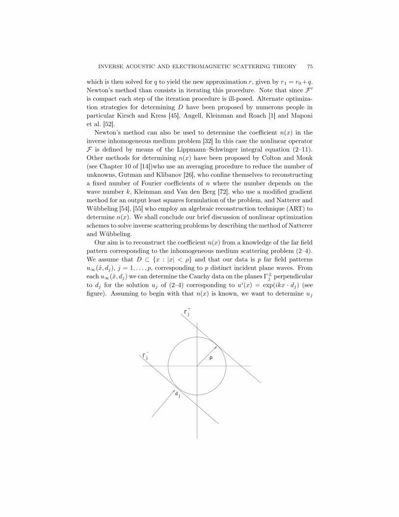
Our aim is to reconstruct the coefficient n(x) from a knowledge of the far field
pattern corresponding to the inhomogeneous medium scattering problem (2–4).
We assume that D ⊂ x : |x| < ρ and that our data is p far field patterns
u∞(x, dj), j = 1, . . . , p, corresponding to p distinct incident plane waves. From
each u∞(x, dj) we can determine the Cauchy data on the planes Γ±j perpendicular
to dj for the solution uj of (2–4) corresponding to ui(x) = exp(ikx · dj) (see
figure). Assuming to begin with that n(x) is known, we want to determine uj
ρΓ
d
−j
j
Γ+j

76 DAVID COLTON
on Γ+j from the ill-posed Cauchy problem
∆uj + k2n(x)uj = 0 in R3, (2–14a)
u = f
∇u · dj = g
on Γ−j ,
on Γ−j
(2–14b)
This can be done in a stable fashion by finite difference methods if we first
filter out frequencies greater than κ where κ < k. We now define the nonlinear
operator Rj : L2(|x| < ρ) → L2(Γ+j ) by
Rj(n) = ujκ
∣
∣
Γ+
J
, (2–15)
where ujκ is the filtered solution of (2–14). Our aim is to now solve the inverse
scattering problem by using an ART-type procedure to solve (2–15) for j =
1, . . . , p.
To solve (2–15) for n we set gj = ujκ
∣
∣
Γ+
j
and solve this equation iteratively by
first determining np from
n0 = n0,
nj = nj−1 + ωR′j(nj−1)
∗C−1j (gj −Rj(nj−1)),
where n0 is an initial guess, ω is a relaxation parameter, R′j is the Frechet
derivative of Rj , Cj = R′j(0)(R′
j(0))∗ where ∗ denotes the adjoint operator and
the operator C−1j can be applied through the use of Fourier transforms (see [54]).
The first approximation is now defined to be np and the procedure is repeated.
For details we refer the reader to Natterer and Wübbeling [54] [55] where the
computational advantages of using such an approach are discussed. An extension
of this method (which is sometimes called the “adjoint field method”) to the case
of time-harmonic electromagnetic waves has been done by Dorn, et.al.[23].
In both the weak scattering and Newton-type methods for solving the inverse
scattering problem we are faced with the problem of solving a linear operator
equation of the form
Aϕ = f
where A : X → Y is compact and X and Y are infinite dimensional normed
spaces. We shall also encounter such equations in the sequel when we consider
linear sampling methods for solving the inverse scattering problem. Hence it is
appropriate to conclude this section of our paper by giving some idea of how
such equations can be solved numerically. The problem in doing this is that
since A is compact solving Aϕ = f is an ill-posed problem in the sense that A−1,
if it exists, is unbounded. This follows immediately from the fact that if A−1
were bounded then I = A−1A is compact, a contradiction since X is infinite
dimensional. Our discussion will purposefully be brief and for more information
on the solution of ill-posed problems we refer the reader to Engl, Hanke and
Neubauer [24], Kirsch [40] and Kress[47].
INVERSE ACOUSTIC AND ELECTROMAGNETIC SCATTERING THEORY 77
We restrict our attention to the case when X and Y are infinite dimensional
Hilbert spaces. We denote by (σn, ϕn, gn) a singular system for the compact
operator A : X → Y , so that
Aϕn = σngn, A∗gn = σnϕn,
and we denote the null space of A by N(A).
Picard’s Theorem. Aϕ = f is solvable if and only if f ∈ N(A∗)⊥ and
∞∑
n=1
1
σ2n
∣
∣(f, gn)∣
∣
2<∞.
In this case a solution is given by
ϕ =∞∑
n=1
1
σn(f, gn)ϕn.
Definition 2.2. The equation Aϕ = f is mildly ill-posed if σn = O(n−β), for
β ∈ R+, and severely ill-posed if the σn decay faster than this.
We note that the equations appearing in inverse scattering theory are typically
severely ill-posed.
For severely ill-posed problems we must use regularization methods to arrive
at a solution.
Definition 2.3. Let A : X → Y be an injective compact linear operator. Then
a family of bounded linear operators Rα : Y → X,α > 0, such that
limα→0
RαAϕ = ϕ
for all ϕ ∈ X is called a regularization scheme for A with regularization parameter
α.
Suppose the solution ϕ of Aϕ = f is approximated by
ϕδα := Rαf
δ
where ‖f − f δ‖ ≤ δ. Then
ϕδα − ϕ = Rαf
δ −Rαf +RαAϕ− ϕ
and hence
‖ϕδα − ϕ‖ ≤ δ‖Rα‖ + ‖RαAϕ− ϕ‖.
The first term in the above equation increases as α tends to zero (since A−1 is
not bounded) whereas the second term is only small when α tends to zero. How
should α = α(δ) be chosen?

78 DAVID COLTON
Definition 2.4. The choice of α = α(δ) is called regular if for all f ∈ A(X)
and all f δ ∈ Y with ‖f − f δ‖ ≤ δ we have
Rα(δ)fδ → A−1f
as δ tends to zero.
We shall now describe a regular regularization scheme due to Tikhonov and
Morozov for solving the ill-posed equation Aϕ = f .
Assume once again that A : X → Y is compact. Then, since A∗A ≥ 0, for
every α > 0 the operator αI + A∗A : X → X is bijective with bounded inverse.
The Tikhonov regularization method for solving Aϕ = f is to set
Rα := (αI +A∗A)−1A∗.
Then the regularized solution ϕα of Aϕ = f is the unique solution of
αϕα +A∗Aϕα = A∗f.
In particular, if A is injective, then
ϕα =
∞∑
n=l
σn
α+ σ2n
(f, gn)ϕn = Rαf
and hence as α tends to zero we have RαAϕ → ϕ for all ϕ ∈ X. The function
ϕα can also be obtained by minimizing the Tikhonov functional
‖Aϕ− f‖2 + α‖ϕ‖2.
Note that if A is injective with dense range then ‖ϕα‖ → ∞ as α tends to zero
if and only if f 6∈ A(X).
We now turn to the choice of the regularization parameter α. If A is injective
with dense range then a regular method for choosing α is the Morozov discrepancy
principle. In particular, assume that we want to solve
Aδϕ = fε
where ‖A − Aδ‖ ≤ δ and ‖f − fε‖ ≤ ε with known δ and ε, i.e. an estimate of
the noise level is known a priori. We require that the residual be commensurate
with the accuracy of the measurements of A and f , i.e.
‖Aδϕα − fε‖ ≈ ε+ δ‖ϕα‖.
In applications to the linear sampling method described in the sequel we have
ε δ. Hence, in this case, the Morozov discrepancy principle is to choose
α = α(δ) such that µ(α) = 0, where
µ(α) := ‖Aδϕα − fε‖2 − δ2‖αα‖2 =
∞∑
n=1
α2 − δ2σ2n
(σ2n + α)2
∣
∣(fε, gn)∣
∣
2

INVERSE ACOUSTIC AND ELECTROMAGNETIC SCATTERING THEORY 79
and (σn, ϕn, gn) is now a singular system for the operator Aδ. We note that µ(α)
is monotonously increasing and in practice only a rough approximation to the
root of µ(α) = 0 is necessary.
In closing this section, we make a few comments on the use of Tikhonov reg-
ularization and the Morozov discrepancy principle in solving ill-posed problems
arising in inverse scattering theory. In particular, we note that in general one
has no idea if the noise level is small enough so that the regularized solution of
the equation with noisy data is in fact a good approximation to the solution of
the noise free equation. Without further a priori information the only statement
that can be made is what happens if the noise tends to zero. However, since
the noise is fixed and nonzero, in general all that can be said is that there is a
“nearby” equation (i.e. noisy A and f) whose solution can be obtained and if
this nearby equation is “close enough” to the noise free equation then one expects
the regularized solution to behave like the true solution, assuming it exists. In
particular, since without severe a priori assumptions, which are in general not
available, error estimates are not known for the dependency of the regularized
solution on the noise level, and the remark of Lanczos is valid: “A lack of in-
formation cannot be remedied by any mathematical trickery.” Nevertheless, a
regularized solution based on Tikhonov regularization and the Morozov discrep-
ancy principle provides a rational approach for arriving at a candidate for a
solution to an ill-posed problem when an a priori estimate of the noise level is
available.
3. The Inverse Dirichlet Problem for Acoustic Waves
In the previous section we discussed two of the most popular methods for
solving the inverse scattering problem, i.e. the weak scattering approximation
and nonlinear optimization techniques, as well as regularization methods that
can be used for their numerical solution. However, as previously mentioned,
both of these methods rely on some a priori knowledge of the physical properties
of the scattering object D in order to know the boundary conditions on ∂D.
Furthermore, uniqueness theorems were not discussed, in particular how much
information is needed in principle to determine D or, more importantly, can
D be determined from the far field data if the boundary conditions are not
known? We view these issues as particularly important since in many practical
inverse scattering problems both the material properties of the scatterer as well
as its shape are unknown. In this and the sections that follow we will be paying
particular attention to inverse scattering problems such as these.
In this section we will consider the inverse scattering problem associated with
the exterior Dirichlet problem (2–3) and, when relevant, point out what results
are in fact independent of the boundary condition on ∂D. We will always assume
the existence of a solution u ∈ C2(R3 \ D) ∩ C(R3 \D) to (2–3) as well as the
fact that since ∂D is in class C2 we have u ∈ C1(R3 \D) [14]. We begin with
80 DAVID COLTON
Rellich’s lemma which forms the basis of the entire field of acoustic scattering
theory.
Theorem 3.1 (Rellich’s lemma). Let us be a solution of the Helmholtz
equation in the exterior of D satisfying the Sommerfeld radiation condition such
that the far field pattern u∞ of us vanishes. Then us = 0 in R3 \ D.
Proof. For sufficiently large |x| we have a Fourier expansion
us(x) =∞∑
n=0
n∑
m=−n
amn (r)Y m
n (x)
with respect to the spherical harmonics Y mn where the coefficients are given by
amn (r) =
∫
Ω
us(rx)Y mn (x) ds(x).
Since us ∈ C2(R3 \ D) and the radiation condition holds uniformly in x, we can
differentiate under the integral sign and integrate by parts to conclude that amn
is a solution of the spherical Bessel equation
d2amn
dr2+
2
r
damn
dr+ (k2 − n(n+ 1)
r2)am
n = 0
satisfying the radiation condition, i.e.
amn (r) = αm
n h(1)n (kr)
where h(1)n is a spherical Hankel function of the first kind of order n and the
αmn are constants depending only on n and m. From (2–7) we have that, since
u∞ = 0,
limr→∞
∫
|x|=r
∣
∣us(x)∣
∣
2ds =
∫
Ω
∣
∣u∞(x)∣
∣
2ds = 0.
But by Parseval’s equality∫
|x|=r
∣
∣us(x)∣
∣
2ds = r2
∞∑
n=0
n∑
m=−n
∣
∣amn (r)
∣
∣
2.
Substituting the above expression for amn into this identity, letting r tend to
infinity, and using the asymptotic behavior of the spherical Hankel functions
now yields αmn = 0 for all n and m. Hence us = 0 outside a sufficiently large
sphere. By the representation formula (2–5) we see that us is an analytic function
of x, and hence we can now conclude that us = 0 in R3 \ D by analyticity. ˜
In the sequel we will need two reciprocity relations which can be proved by a
straightforward application of Green’s theorem. The first of these is for scattering
by a plane wave, i.e. ui(x) = eikx·d in (2–3), and is given by [14]
u∞(x, d) = u∞(−d,−x) (3–1)

INVERSE ACOUSTIC AND ELECTROMAGNETIC SCATTERING THEORY 81
and the second of these is for scattering due to the point source ui(x) = Φ(x, z)
having far field pattern u∞(x, z) and is given by [62]
4πu∞(−d, z) = us(z, d) (3–2)
for z ∈ R3 \ D, d ∈ Ω, where us is the scattered field in (2–3) corresponding to
ui(x) = eikx·d.
We now consider the scattering problem (2–3) and let u∞ be the far field
pattern of the scattered field. The far field operator F : L2(Ω) → L2(Ω) for this
problem is defined by
(Fg)(x) :=
∫
Ω
u∞(x, d)g(d) ds(d) (3–3)
and is easily seen to be the scattered field vsg corresponding to the Herglotz wave
function
vig(x) :=
∫
Ω
eikx·dg(d) ds(d), x ∈ R3
as incident field. The function g ∈ L2(Ω) is known as the kernel of the Herglotz
wave function. Of basic importance to us is the following theorem [14].
Theorem 3.2. The far field operator F is injective with dense range if and only
if there does not exist a Dirichlet eigenfunction for D which is a Herglotz wave
function.
Proof. For the L2 adjoint F ∗ : L2(Ω) → L2(Ω) the reciprocity relation (3–1)
implies that
F ∗g = RFRg (3–4)
where R : L2(Ω) → L2(Ω) is defined by
(Rg)(d) := g(−d).
Hence, the operator F is injective if and only if its adjoint F ∗ is injective. Re-
calling that the denseness of the range of F is equivalent to the injectivity of
F ∗ we therefore must only show the injectivity of F . To this end, we note that
Fg = 0 with g 6= 0 is equivalent to the existence of a nontrivial Herglotz wave
function vig with kernel g for which the far field pattern of the corresponding
scattered field vs is v∞ = 0. By Rellich’s lemma this implies vs = 0 in R3 \Dand the boundary condition vi
g + vs = 0 on ∂D now shows that vig = 0 on ∂D.
The proof is finished. ˜
We now want to show that the far field F is normal. To this end, we need the
following lemma [15].
Lemma 3.3. The far field operator F satisfies
2π(
(Fg, h) − (g, Fh))
= ik(Fg, Fh).

82 DAVID COLTON
Proof. If vs and ws are radiating solutions to the Helmholtz equation with
far field patterns v∞ and w∞ then from the radiation condition and Green’s
theorem we obtain∫
∂D
(
vs ∂ws
∂ν− ws
∂vs
∂ν
)
ds = −2ik
∫
Ω
v∞w∞ ds.
From the representation formula (2–5) and letting x → ∞ we see that, if wih is
a Herglotz wave function with kernel h, then
∫
∂D
(
vs(x)∂wi
h
∂ν(x) − wi
h(x)∂vs
∂ν(x)
)
ds(x)
=
∫
Ω
h(d)
∫
∂D
(vs(x)∂e−ikx·d
∂ν− e−ikx·d ∂v
s
∂ν(x)) ds(x) ds(d)
= 4π
∫
Ω
h(d)v∞(d) ds(d).
Now let vig and vi
h be Herglotz wave functions with kernels g, h ∈ L2(Ω),
respectively, and let vg, vh be the solutions of (2–3) with ui replaced by vig and
vih, respectively. Let vg,∞ and vh,∞ be the corresponding far field patterns. Then
we can combine the two previous equations to obtain
−2ik(Fg, Fh) + 4π(Fg, h) − 4π(g, Fh)
= −2ik
∫
Ω
vg,∞vh,∞ ds+ 4π
∫
Ω
vg,∞h ds− 4π
∫
Ω
gvh,∞ ds
=
∫
∂D
(
vg∂vh
∂ν− vh
∂vg
∂ν
)
ds
and the lemma follows from the Dirichlet boundary condition satisfied by vg
and vh. ˜
Theorem 3.4. The far field operator F is compact and normal .
Proof. Since F is an integral operator on Ω with a continuous kernel, it is
compact. From Lemma 3.3 we have
(g, ikF ∗Fh) = 2π(
(g, Fh) − (g, F ∗h))
for all g, h ∈ L2(Ω) and hence
ikF ∗F = 2π(F − F ∗). (3–5)
Using (3–4) we can deduce that
(F ∗g, F ∗h) = (FRh, FRg)
INVERSE ACOUSTIC AND ELECTROMAGNETIC SCATTERING THEORY 83
and hence from Lemma 3.3 again it follows that
ik(F ∗g, F ∗h) = 2π(
(g, F ∗h) − (F ∗g, h))
for all g, h ∈ L2(Ω). If we now proceed as in the derivation of (3–6) we find that
ikFF ∗ = 2π(F − F ∗) (3–6)
and the proof is finished. ˜
The proof of Theorem 3.4 carries over to the case of Neumann boundary data.
However for the impedance boundary condition
∂u
∂ν+ ikλu = 0
where λ > 0 the operator F is no longer normal since Lemma 3.3 is not valid,
i.e. absorption destroys normality. Finally, returning to the case of Dirichlet
boundary data, if we define the scattering operator S : L2(Ω) → L2(Ω) by
S = I +ik
2πF
then from (3–5) and (3–6) we see that SS∗ = S∗S = I, i.e., S is unitary.
Having established the basic properties of the far field pattern and far field
operator, we now turn our attention to the uniqueness of a solution to the inverse
scattering problem, basing our analysis on the approach of Kirsch and Kress [46]
with a subsequent simplification of the proof by Potthast [62].
Theorem 3.5. Assume that D1 and D2 are two obstacles such that the far field
patterns corresponding to the exterior Dirichlet problem (2–3) for D1 and D2
coincide for all incident directions d. Then D1 = D2.
Proof. By analyticity and Rellich’s lemma the scattered fields us1( · , d) =
us2( · , d) for the incident fields ui(x, d) = eikx·d coincide in the unbounded com-
ponent G of the complement of D1 ∪ D2 for all d ∈ Ω. Then from the reciprocity
relation (3–2) we can conclude that the far field patterns u1,∞( · , z) = u2,∞( · , z)for the scattering of point sources Φ( · , z) coincide for all point sources located at
z ∈ G. Again by Rellich’s lemma, this implies that the corresponding scattered
fields satisfy us1(x, z) = us
2(x, z) for all x, z ∈ G.
Now assume that D1 6= D2. Then, without loss of generality, there exists
x∗ ∈ ∂G such that x∗ ∈ ∂D1 and x∗ 6∈ D2. In particular, we have
zn := x∗ +1
nν(x∗)
is in G for integers n sufficiently large. Then, on the one hand, we have
limn→∞
us2(x
∗, zn) = us2(x
∗, x∗)

84 DAVID COLTON
since us2(x
∗, ·) is continuous in a neighborhood of x∗ 6∈ D2 due to the well-
posedness of the direct scattering problem. On the other hand, we have
limn→∞
us1(x
∗, zn) = ∞
because of the boundary condition us1(x
∗, zn) + Φ(x∗, zn) = 0. This contradicts
the fact that us1(x
∗, zn) = us2(x
∗, zn) for n sufficiently large and the proof in
complete. ˜
A closer examination of the proof of Theorem 3.5 shows that the boundary
condition u = 0 is not used explicitly but rather only the well-posedness of
the direct scattering problem. Hence it is not necessary to know the boundary
condition (2–3d) a priori in order to conclude that the far field pattern uniquely
determines the scatterer. In fact it is not even necessary to know if u∞ is the
far field pattern of (2–2), (2–3) or (2–4) in order to conclude that D is uniquely
determined [41], [42]. In a related direction, Potthast [62], [64] has considered
the important case of finite data. In particular, if Ωn ⊂ Ω is a set of n uniformly
distributed unit vectors such that if
d(x,Ωn) := infd∈Ωn
|x− d|
then (1) d(x,Ωn) → 0 as n → ∞; (2) d ∈ Ωn =⇒ −d ∈ Ωn if n is even; and (3)
Ωn′ ,⊂ Ωn for n > n′ then the following theorem is valid.
Theorem 3.6. Let u∞1 and u∞2 be the far field patterns corresponding to one of
(2–2), (2–3) or (2–4). Given ε > 0 there exists integers n0 and ni such that if
u∞1 (x, d) = u∞2 (x, d) for x ∈ Ωn0, d ∈ Ωni
then
d(D1,D2) ≤ ε,
where d(D1,D2) denotes the Hausdorff distance between D1 and D2.
An open problem is to determine if one incident plane wave at a fixed wave
number k is sufficient to uniquely determine the scatterer D. If it is known a
priori that the boundary condition (2–3d) is satisfied and that furthermore D is
contained in a ball of radius R such that kR < π then it was shown by Colton
and Sleeman ([20] and Corollary 5.3 of [14]) that D is uniquely determined by
its far field pattern for a single incident direction d and fixed wave number k.
We now turn our attention to a method for reconstructing D from an inexact
knowledge of the far field pattern u∞ of the scattering problem (2–3) that is
closely related to the ideas of the proof of the uniqueness Theorem 3.5. Indeed,
as with Theorem 3.5, this method can be implemented without knowing a priori
which of the scattering problems (2–2), (2–3) or (2–4) is associated with u∞ and
in this sense has a clear advantage over the reconstruction methods discussed in
the previous section. On the other hand, the implementation requires a knowl-
edge of u∞(x, d) for x, d on open subsets of Ω whereas for obstacle scattering
Newton’s method only requires a single incident direction d. Furthermore, for

INVERSE ACOUSTIC AND ELECTROMAGNETIC SCATTERING THEORY 85
the case of the scattering problem (2–4), only the support D is obtained rather
than the coefficient n(x). The method we have on mind was first introduced
by Colton and Kirsch in [12], with a subsequent second version being given by
Kirsch in [42] and [43] and has become known as the linear sampling method
(related methods have been considered by Ikehata [35], Norris [56] and Potthast
[65]). Here, for the sake of simplicity, we will assume that u∞(x, d) is known for
all x, d ∈ Ω rather than only on a subset of Ω. For the case of the first version of
the linear sampling method, this latter case can be easily handled by appealing
to the result that a Herglotz wave function and its first derivatives can be ap-
proximated on compact subsets of a ball B by another Herglotz wave function
having a kernel that is compactly supported on Ω. (This can easily be shown by
assuming without loss of generality that k2 is not a Dirichlet eigenvalue for B
and then using the ideas of the proof of Theorem 5.5 of [14] to show that Herglotz
wave functions with compactly supported kernels are dense in L2(∂B)).
To describe the basic idea behind the linear sampling method, assume that
for every z ∈ D there exists a unique solution g = g( · , z) ∈ L2(Ω) to the far
field equation∫
Ω
u∞(x, d)g(d) ds(d) = Φ∞(x, z), (3–7)
where
Φ∞(x, z) =1
4πe−ikx·z
and u∞ is the far field pattern corresponding to the scattering problem (2–3).
Then, since the right hand side of (3–7) is the far field pattern of the fundamental
solution Φ(x, z), it follows from Rellich’s lemma that∫
Ω
us(x, d)g(d) ds(d) = Φ(x, z)
for x ∈ R3 \D. From the boundary condition u = 0 on ∂D it now follows that
vig(x) + Φ(x, z) = 0 for x ∈ ∂D, (3–8)
where vig is the Herglotz wave function with kernel g. We now see from (3–8)
that vig becomes unbounded as z → x ∈ ∂D and hence
limz→∂Dz∈D
∥
∥g( · , z)∥
∥ = ∞,
that is, ∂D is characterized by points z where the solution of (3–7) becomes
unbounded.
Unfortunately, in general the far field equation
Fg = Φ∞( · , z)
does not have a unique solution, nor does the above analysis say anything about
what happens when z ∈ R3 \D. However, using on the one hand the fact that

86 DAVID COLTON
Herglotz wave functions are dense in the space of solutions to the Helmholtz
equation in D with respect to the norm in the Sobolev space H1(D) (see [16],
[21]) and on the other the factorization of the far field operator F as
(Fg) = − 1
4πFS−1(Hg),
where S : H−1/2(∂D) → H1/2(∂D) is the single layer potential
(Sϕ)(x) :=
∫
∂D
ϕ(y)Φ(x, y) ds(y), (3–9)
Hg is the trace on ∂D of the Herglotz wave function, and F : H−1/2(∂D) →L2(Ω) is defined by
(Fϕ)(x) :=
∫
∂D
ϕ(y)ϕ−ikx·y ds(y),
we can prove the following result [4].
Theorem 3.7. Assume that k2 is not a Dirichlet eigenvalue for D. Then
(1) if z ∈ D for every ε > 0 there exists a solution g( · , z) ∈ L2(Ω) of the
inequality∥
∥Fg( · , z) − Φ∞( · , z)∥
∥ < ε
such that
limz→∂D
∥
∥g( · , z)∥
∥
L2(Ω)= ∞, lim
z→∂D
∥
∥vig( · , z)
∥
∥
H1(D)= ∞,
(2) if z ∈ R3\D for every ε > 0 and γ > 0 there exists a solution g( · , z) ∈ L2(Ω)
of the inequality∥
∥Fg( · , z) − Φ∞( · , z)∥
∥ < ε+ γ
such that
limγ→0
‖g( · , z)‖L2(Ω) = ∞, limγ→0
∥
∥vig( · , z)
∥
∥
H1(D)= ∞.
We note that the difference between cases (1) and (2) of this theorem is that,
for z ∈ D, Φ∞( · , z) is in the range of F whereas for z ∈ R3 \ D this is no longer
true.
The above theorem now suggests a numerical procedure for determining ∂D
from noisy far field data. In particular, let uδ∞ be the measured far field data,
i.e. ‖uδ∞−u∞‖ < δ and assume g is such that
∥
∥Fg−Φ∞( · , z)∥
∥ < ε. If Fδ is the
operator F with kernel u∞ replaced by uδ∞, then we want to find an approxima-
tion to g by solving Fδϕ = Φ∞( · , z); that is, we view both the operator and the
right hand side as being inexact. This equation is now solved using Tikhonov
regularization and the Morozov discrepancy principle. The unknown boundary
∂D is now determined by looking for those points z where∥
∥ϕ( · , z)∥
∥ begins to

INVERSE ACOUSTIC AND ELECTROMAGNETIC SCATTERING THEORY 87
sharply increase. Numerical examples using this procedure can be found in [9],
[10] and [74].
The analogue of Theorem 3.7 for the exterior Neumann problem is established
in exactly the same way as Theorem 3.7 where now it is assumed that k2 is
not a Neumann eigenvalue for D. It is also possible to treat mixed boundary
value problems [4], [6]. As will be seen in the next section, a similar result also
holds for the inhomogeneous medium problem (2–4) as well as the more general
problem (2–1) provided k2 is not a transmission eigenvalue (to be defined in the
following section of this paper). In particular, as with Theorems 3.5 and 3.6,
it is not necessary to know the material properties of the scatterer (e.g., the
boundary condition) in order to determine D from a knowledge of the regularized
solution of the far field equation. it is also possible to treat the case when the
background medium is piecewise homogeneous by appropriately modifying the
far field equation [9]. The possibility of doing this is particularly important in
numerous applications, e.g. the detection of buried objects or structures under
foliage.
Theorem 3.7 is complicated by the fact that in general Φ∞( · , z) is not in the
range of F for neither z ∈ D nor z ∈ R3 \ D. For the case when F is normal
(say nonabsorbing media and data on all of Ω rather than some subset of Ω),
this problem was resolved by Kirsch [42], who proposed replacing the equation
Fg = Φ∞( · , z) by (F ∗F )14 g = Φ∞( · , z) where F ∗ is again the adjoint of F in
L2(Ω). He was then able to show that Φ( · , z) is in the range of (F ∗F )14 if and
only if z ∈ D. We will now outline the main ideas of Kirsch’s proof of this result.
In what follows, S : L2(∂D) → L2(∂D) is the single layer potential defined by
(3–9) and G : L2(∂D) → L2(Ω) is defined by Gh = v∞ where v∞ is the far field
pattern of the solution to the radiating exterior Dirichlet problem with boundary
data h ∈ L2(∂D). The relation among the operators F,G and S is given by the
following lemma.
Lemma 3.8. The relation
F = −4πGS∗G∗
is valid where G∗ : L2(Ω) → L2(∂D) and S∗ : L2(∂D) → L2(∂D) are the L2
adjuncts of G and S respectively .
Proof. Define the operator H : L2(Ω) → L2(∂D) by
(Hg)(x) :=
∫
Ω
g(d)eikx·d ds(d).
Note that Hg is the Herglotz wave function with density g. The adjoint operator
H∗ : L2(∂D) → L2(Ω) is given by
(H∗ϕ)(x) =
∫
∂D
ϕ(y)e−ikx·y ds(y)

88 DAVID COLTON
and we note that 14πH
∗ϕ is the far field pattern of the single layer potential (3–9).
The single layer potential with continuous density ϕ is continuous in R3 and thus14πH
∗ϕ = GSϕ , i.e. by a denseness argument
H = 4πS∗G∗ (3–10)
on L2(∂D). We now observe that Fg is the far field pattern of the solution to
the radiating exterior Dirichlet problem with boundary data −(Hg)(x), x ∈ ∂D,
and hence
Fg = −GHg. (3–11)
Substituting (3–10) into (3–11) now yields the lemma. ˜
We now assume that k2 is not a Dirichlet eigenvalue for D. Then by Theorems
3.2 and 3.4 the far field operator F is normal and injective. In particular, there
exists eigenvalues λj ∈ C of F, j = 1, 2, . . ., with λj 6= 0, and the corresponding
eigenfunctions ψj ∈ L2(ω) form a complete orthonormal system in L2(Ω). From
Lemma 3.3 we can deduce the fact that the λj all lie on the circle of radius 2πk
and center 2πik . We also note that |λj |, ψj , sign (λj)ψj is a singular system for
F . By the preceding lemma,
−4πGS∗G∗λj = λjψj .
If we define the functions ϕj ∈ L2(∂D) by
G∗ψj = −√
λjϕj ,
where we choose the branch of√
λj such that Im√
λj > 0, we see that
GS∗ϕj =
√
λj
4πψj . (3–12)
A central result of Kirsch is that the functions ϕj form a Riesz basis in the
Sobolev space H−1/2(∂D), i.e. H−1/2(∂D) consists exactly of functions ϕ of the
form
ϕ =
∞∑
j=1
αjϕj with∞∑
j=1
|αj |2 <∞.
The proof of this result relies in a fundamental way on the normality of F . Using
these results we can now prove the main result of [42] where in the proof of the
theorem R(A) denotes the range of the operator A.
Theorem 3.9. Assume that k2 is not a Dirichlet eigenvalue for D. Then the
ranges of G : H1/2(∂D) → L2(Ω) and (F ∗F )14 : L2(Ω) → L2(Ω) coincide.
Proof. We use the fact that S∗ : H−1/2(∂D) → H1/2(∂D) is an isomorphism.
Suppose Gϕ = ψ for some ϕ ∈ H1/2(∂D). Then (S∗)−1ϕ ∈ H−1/2(∂D) and thus
(S∗)−1ϕ =∑∞
j=1 αjϕj with∑∞
j=1 |αj |2 <∞. Therefore, by (3–12), we have
ψ = Gϕ = GS∗(S∗)−1ϕ =1
4π
∞∑
j=1
αj
√
λjψj =
∞∑
j=1
ρjψj

INVERSE ACOUSTIC AND ELECTROMAGNETIC SCATTERING THEORY 89
with ρj = 14παj
√
λj and thus
∞∑
j=1
|ρj |2|λj |
=1
(4π)2
∞∑
j=1
|αj |2 <∞. (3–13)
On the other hand, let ψ =∑∞
j=1 ρjψj with the ρj satisfying (3–13) and define
ϕ :=∑∞
j=1 αjϕj with αj = 4πρj/√
λj . Then∑∞
j=1 |αj |2 < ∞ and hence ϕ ∈H−1/2(∂D), S∗ϕ ∈ H1/2(∂D), and
G(S∗ϕ) =1
4π
∞∑
j=1
αj
√
λjψj =∞∑
j=1
ρjψj = ψ.
Since√
|λj | and ψj are the eigenvalues and eigenfunctions, respectively, of the
self-adjoint operator (F ∗F )14 , we have
R(F ∗F )14 =
( ∞∑
j=1
ρjψj :∞∑
j=1
|ρj |2|λj |
<∞)
,
and, as we have shown above, this is precisely R(G). ˜
Since Φ∞(x, z) = 14π e
−ikx·z is the far field pattern of the fundamental solution
Φ(x, z), it is easy to verify that Φ∞( · , z) is in the range of G and if and only if
z ∈ D, i.e. (F ∗F )14 g = Φ∞( · , z) is solvable if and only if z ∈ D. In particular, if
regularization methods are used to solve (F ∗F )14 g = Φ∞( · , z) then from Section
2 of this paper we see that as the noise level on u∞ tends to zero the norm of the
regularized solution remains bounded if and only if z ∈ D. Numerical examples
using this procedure can be found in [10] and [42].
Under the assumption that k2 is not a Neumann eigenvalue, the equation
(F ∗F )14 g = Φ∞( · , z) can also be derived for the determination of D, i.e. it is
not necessary to know a priori whether or not the boundary data is of Dirichlet or
Neumann type. However, in both cases the derivation of this equation depends
on F being a normal operator. In particular this excludes the limited aperature
case when Ω is replaced by a subset Ω0 of Ω as well as the case of impedance
boundary data. In an effort to avoid this problem, Kirsch has introduced a
simple nonlinear optimization scheme which preserves some of the advantages of
the second version of the linear sampling method while at the same time avoiding
the assumption of normality of F [44]. We will conclude this section of our paper
by describing Kirsch’s optimization scheme.
The optimization scheme of Kirsch is based on the following theorem.
Theorem 3.10. Let X1 be a (complex ) reflexive Banach space with dual X∗1
and dual form 〈 · , · 〉1. Let X2 be a (complex ) Hilbert space with inner product
〈 · , · 〉2 and F : X2 → X2, B : X1 → X2, compact linear operators such that B is
injective. Suppose there exists a bounded linear operator A : X∗1 → X1 such that
F = BAB∗ and
c1‖Aϕ‖21 ≤
∣
∣〈ϕ,Aϕ〉1∣
∣≤ c2‖Aϕ‖21 (3–14)

90 DAVID COLTON
for all ϕ ∈ X∗1 where c1 and c2 are positive constants. Then for any ϕ ∈ X2, ϕ 6=
0, ϕ ∈ R(BA∗) if and only if
inf∣
∣〈ψ,Fψ〉2∣
∣: ψ ∈ X2, 〈ψ,ϕ〉2 = 1
> 0.
Proof. From (3–14), we have∣
∣〈ψ,Fψ〉2∣
∣ =∣
∣〈B∗ψ, AB∗ψ〉1∣
∣ ≥ c1‖AB∗ψ‖2,
for all ψ ∈ X2. Let ϕ = BA∗ϕ0 for some ϕ0 ∈ X∗1 . Then for ψ ∈ X2 such that
〈ψ,ϕ〉2 = 1 we have
∣
∣〈ψ,Fψ〉2∣
∣ ≥ c1‖AB∗ψ‖21 =
c1‖ϕ0‖2
1
‖AB∗ψ‖21 ‖ϕ0‖2
1
≥ c1‖ϕ0‖2
1
|〈ϕ0, AB∗ψ〉1|2 =
c1‖ϕ0‖|21
|〈BA∗ϕ0, ψ〉2|2 =c1
‖ϕ0|21> 0.
Now assume that ϕ 6= R(BA∗) and define the closed subspace V := ψ ∈ X2 :
〈ψ,ϕ〉2 = 0. We will show that AB∗(V ) is dense in R(A) = N(A∗)⊥. To see
this, let ϕ ∈ X∗1 such that 〈ϕ,AB∗ψ〉1 = 0 for all ψ ∈ V . Then 〈BA∗ϕ,ψ〉2 = 0
for all ψ ∈ V , i.e., BA∗ϕ ∈ V ⊥ = spanϕ. Since ϕ ∈ R(BA∗) this implies that
BA∗ϕ = 0 and hence A∗ϕ = 0 by the injectivity of B. Therefore ϕ ∈ N(A∗) =
R(A)⊥ and hence AB∗(V ) is dense in R(A). We can therefore find a sequence
ψn in V such that
AB∗ψn → − 1
‖ϕ‖22
AB∗ϕ
as n→ ∞. We now set ψn = ψn +ϕ/‖ϕ‖22. Then 〈ψn, ϕ〉2 = 1 and AB∗ψn → 0.
From (3–14) we have∣
∣〈ψn, Fψn〉2∣
∣ =∣
∣〈B∗ψ,AB∗ψ〉1∣
∣ ≤ c2‖AB∗ψn‖21
and hence 〈ψn, Fψn〉2 → 0 as n→ ∞, i.e.,
inf
|〈ψ,Fψ〉2| : ψ ∈ X2, 〈ψ,ϕ〉2 = 1
= 0. ˜
In order to make use of Theorem 3.10, Kirsch defines G : H1/2(∂D) → L2(Ω)
and S : H−1/2(∂D) → H1/2(∂D) as in Lemma 3.8 (with the indicated changes
in ranges and domains) and proves that if F : L2(Ω) → L2(Ω) is the far field op-
erator corresponding to the exterior Dirichlet problem (2–3) then we again have
the factorization F = 4πGS∗G∗. After showing that S∗ satisfies the coercivity
condition (3–14) if k2 is not a Dirichlet eigenvalue, and using the fact that in this
case S is an isomorphism, it is then possible to use Theorem 3.10 to conclude
that if k2 is not a Dirichlet eigenvalue we have
ϕ ∈ R(G) ⇐⇒ inf∣
∣〈ψ,Fψ〉L2(Ω)
∣
∣ : ψ ∈ L2(Ω), 〈ϕ,ψ〉L2(Ω) = 1
> 0.
Since z ∈ D if and only if Φ∞( · , z) ∈ R(G) we now have the following theorem
[44].

INVERSE ACOUSTIC AND ELECTROMAGNETIC SCATTERING THEORY 91
Theorem 3.11. Assume that k2 is not a Dirichlet eigenvalue. Then
z ∈ D ⇐⇒ inf
|〈ψ,Fψ〉| : ψ ∈ L2(Ω), 〈Φ∞( · , z), ψ〉L2(Ω) = 1
> 0.
Theorem 3.11 leads in an obvious manner to a constrained optimization scheme
for determining when a point z ∈ R3 is in D [44]. Note that the proof of Theorem
3.11 does not rely on the normality of F .
4. The Inverse Medium Problem for Acoustic Waves
We will now turn our attention to inverse scattering problems associated with
the inhomogeneous medium problem (2–4) and ultimately the acoustic transmis-
sion problem (2–1). As in Section 3, we will focus our attention on the situation
where neither the material properties of the scatterer nor its shape are known.
Then it follows from the uniqueness theorems of Nachman [53] and Isakov [36],
[37]that for a single frequency the best that we can hope for is to determine the
shape D of the scatterer. In particular, in order to determine the coefficients
in (2–1b), either multi-frequency data is needed or an a priori knowledge of ei-
ther ρD(x) or n(x) is required. If such information is available then nonlinear
optimization techniques such as those described in Section 2 of this paper can
be used to determine the coefficients. Here we will restrict ourselves to a fixed
frequency and prove uniqueness theorems associated with the direct scattering
problems (2–1) and (2–4) as well as reconstruction algorithms for determining
D from the far field pattern u∞.
In the previous section we presented three different methods for determining
the shape D of the scatterer from a knowledge of the far field pattern associ-
ated with the exterior Dirichlet problem (2–3), in particular the two versions of
the linear sampling method based on F and (F ∗F )14 respectively and the con-
strained optimization method based on Theorem 3.11. Each of these methods,
under appropriate assumptions, can be extended to the inverse scattering prob-
lem associated with the inhomogeneous medium problems (2–4) [12], [19], [43],
[44]. However, at the time of writing, only the linear sampling method asso-
ciated with the far field operator F has been extended to the general acoustic
transmission problem (2–1) [6], [7] and the case of Maxwell’s equations [11], [29],
[49]. Hence, in the interest of developing a unifying theme to our paper, we will
restrict our attention to the first version of the linear sampling method in order
to determine D.
We begin our discussion by considering the inhomogeneous medium problem
(2–4) and again define the far field operator F : L2(Ω) → L2(Ω) by
(Fg)(x) :=
∫
Ω
u∞(x, d)g(d) ds(d), (4–1)
where u∞ is the far field pattern of the scattered field us defined in (2–4). It is
again possible to establish the reciprocity relations (3–1) and (3–2). However,

92 DAVID COLTON
since Imn(x) ≥ 0, we cannot expect normality of F except in the case when
Imn(x) = 0. The question of when F is injective with dense range is addressed
by the following theorem, where the role of the interior Dirichlet problem in
Theorem 3.2 is now replaced by a new type of boundary value problem called
the homogeneous interior transmission problem.
Theorem 4.1. The far field operator F defined by (4–1) is injective with dense
range if and only if there does not exist w ∈ C2(D)∩C2(D) and a Herglotz wave
function v with kernel g 6= 0 such that v, w is a solution to the homogeneous
interior transmission problem
∆v + k2v = 0
∆w + k2n(x)w = 0
in D,
in D,(4–2a)
v = w
∂w
∂ν
on ∂D,
on ∂D.(4–2b)
Proof. As in the case of Theorem 3.2, it suffices to establish conditions for
when the far field operator is injective. To this end, we note that Fg = 0 with
g 6= 0 is equivalent to the vanishing of the far field pattern of ws where w is the
solution of (2–4) with ui a Herglotz wave function v with kernel g. By Rellich’s
lemma, ws = 0 in R3 \D, and hence if w = v + ws we have
w = v on ∂D,∂w
∂ν=∂v
∂νon ∂D. ˜
An elementary application of Green’s theorem and the unique continuation prin-
ciple for elliptic equations shows (Theorem 8.12 of [14]) that if Imn(x0) > 0 for
some x0 ∈ D then the only solution of (4–2) is v = w = 0, i.e., in this case F is
injective with dense range. Knowing that the values of k for which the far field
operator is not injective form a discrete set is of considerable importance in the
inverse scattering problem associated with (2–4), just as it is in the case of the
obstacle problem (2–3) where it is known that the set of Dirichlet eigenvalues
forms a discrete set. In the case of the linear sampling method, for example, this
enables us to conclude that the method can fail only for a discrete set of values of
k. From Theorem 4.1 we see that F is injective if there does not exist a nontriv-
ial solution to the homogeneous interior transmission problem. Values of k for
which there exists a nontrivial solution to the homogeneous interior transmission
problem are called transmission eigenvalues. It was shown by Colton, Kirsch and
Päivärinta ([13] and Section 8.6 of [14]) and by Rynne and Sleeman [67] that if
there exists ε > 0 such that either n(x) ≥ 1 + ε for x ∈ D or 0 < n(x) ≤ 1 − ε
for x ∈ D then the set of transmission eigenvalues is discrete.
We now turn to the problem of the unique determination of n(x) in (2–4)
from a knowledge of the far field pattern u∞(x, d) for x, d ∈ Ω. The original
proof of this result is due to Nachman [53], Novikov [57] and Ramm [66] and is

INVERSE ACOUSTIC AND ELECTROMAGNETIC SCATTERING THEORY 93
based on the fundamental paper of Sylvester and Uhlmann [71]. Here we follow
a modification of the original proof due to Hähner [30] which is based on the
following two lemmas, where H2(B) denotes a Sobolev space.
Lemma 4.2. Let B be an open ball centered at the origin and containing the
support of m := 1−n. Then there exists a positive constant C such that for each
z ∈ C3 with z · z = 0 and |Re z| ≥ 2k2‖n‖∞ there exists a solution w ∈ H2(B)
to ∆w + k2nw = 0 in B of the form
w(x) = eiz·x(
1 + r(x))
,
where
‖r‖L2(B) ≤C
|Re z| .
Lemma 4.3. Let B1 and B2 be two open balls entered at the origin and containing
the support of m := 1 − n such that B1 ⊂ B2. Then the set of total fields
u( · , d), d ∈ Ω satisfying (2–4) is complete in the closure of
H := w ∈ C2(B2) : ∆w + k2nw = 0 in B2
with respect to the norm in L2(B1).
We are now ready to prove the following uniqueness result for the inverse inho-
mogeneous medium problem (2–4).
Theorem 4.4. The coefficient n(x) in (2–4) is uniquely determined by a knowl-
edge of the far field pattern u∞(x, d) for x, d ∈ Ω.
Proof. Assume that n1 and n2 are such that u1,∞( · , d) = u2,∞( · , d), d ∈ Ω,
and let B1 and B2 be two open balls centered at the origin and containing the
supports of 1 − n1 and 1 − n2 such that B1 ⊂ B2. Then by Rellich’s lemma we
have u1( · , d) = u2( · , d) in R3 \ B1 for all d ∈ Ω. Hence u = u1 − u2 satisfies
u = ∂u/∂ν on ∂B1 and the differential equation
∆u+ k2n1u = k2(n2 − n1)u2
in B1. From this and the differential equation for u1 = u1( · , d), d ∈ Ω, we obtain
k2u1u2(n2 − n1) = u1(∆u+ k2n1u) = u1∆u− u∆u1.
From Green’s theorem and the fact that the Cauchy data for u vanishes on ∂B1
we now have∫∫
B1
u1( · , d)u2( · , d)(n1 − n2) dx = 0
for all d, d ∈ Ω. It now follows from Lemma 4.3 that∫∫
B1
w1w2(n1 − n2) dx = 0 (4–3)
94 DAVID COLTON
for all solutions w1, w2 ∈ C2(B2) of ∆w1 + k2n1w1 = 0 and ∆w2 + k2n2w2 = 0
in B2.
Given y ∈ R3 \ 0 and ρ > 0, we now choose vectors a, b ∈ R3 such that
y, a, b is an orthogonal basis in R3 with the properties that |a| = 1 and |b|2 =
|y|2 + ρ2. Then for z1 := y + ρa+ ib, z2 := y − ρa− ib we have
zj · zj = |Re zj |2 − |Im zj |2 + 2iRe zj · Im zj = |y|2 + ρ2 − |b|2 = 0
and |Re zj |2 = |y|2 + ρ2 ≥ ρ2. In (4–3) we now substitute the solutions w1
and w2 from Lemma 4.2 for the coefficients n1 and n2 and vectors z1 and z2,
respectively. Since z1 + z2 = 2y this gives∫∫
B1
e2iy·x(
1 + r1(x))(
1 + r2(x))(
n1(x) − n2(x))
dx = 0
and, passing to the limit as ρ→ ∞, gives∫∫
B1
e2iy·x(
n1(x) − n2(x))
dx = 0.
Since this equation is true for arbitrary y ∈ R3, by the Fourier integral theorem
we have n1(x) = n2(x) in B1 and the proof is finished. ˜
Before proceeding to reconstruction algorithms for determining the support of
m = 1 − n, we note that at the time of writing a uniqueness theorem for the
inverse inhomogeneous medium problem (2–4) in R2 analogous to Theorem 4.4
for the case of R3 is unknown. The problem in R2 is more difficult than the case
in R3 due to the fact that the inverse scattering problem for fixed frequency in R2
is not overdetermined as in the R3 case. i.e., in R2, u∞(x, d) is a function of two
variables and n(x) is also a function of two variables. Nevertheless, there have
been numerous partial results in this case due to Novikov [58], Sun and Uhlmann
[68], Isakov and Nachman [38], Isakov and Sun [39] and Eskin [25] among others.
We content ourselves here by stating a single result in this direction due to Sun
and Uhlmann [70] (see also [64]) which shows that the discontinuities of n are
uniquely determined from the far field pattern u∞. We note that in the R2 case
the radiation condition (2–4c) is replaced by
limr→∞
r1/2(∂us
∂r− ikus
)
= 0
and the asymptotic behavior (2–7) is replaced by
us(x) =eikr
√ru∞(x, d) +O(r−3/2).
Theorem 4.5. Let n1 and n2 be in L∞(R2) and suppose m1 := 1−n1 and m2 :=
1 − n2 have compact support . Then if uj∞ is the far field pattern corresponding
to nj for j = 1, 2 and u1∞(x, d) = u2
∞(x, d) for all x, d on the unit circle Ω, then
n1 − n2 ∈ C0,α(R2) for every α, 0 ≤ α < 1.

INVERSE ACOUSTIC AND ELECTROMAGNETIC SCATTERING THEORY 95
We now return to the three dimensional inverse scattering problem associated
with (2–4). Given the fact that n(x) is uniquely determined from u∞, we can
now attempt to reconstruct n(x) by using nonlinear optimization techniques as
discussed in Section 2 of this paper. (A reconstruction procedure for determining
n based on the techniques used in the uniqueness Theorem 4.4 has been given
by Nachman [53] and Novikov [57] although it is not clear whether or not this
leads to a viable numerical procedure.) However, a reconstruction of n(x) is
often more than is necessary. Indeed, it is frequently sufficient to determine the
support of m = 1−n and, as mentioned at the beginning of this section, for fixed
frequency and the more general acoustic transmission problem this is essentially
all the information that can be extracted from the far field data u∞. We will
now proceed to show how the linear sampling method can be used to determine
the support D of m := 1 − n basing our analysis on the ideas of Colton and
Kirsch [12] and Colton, Piana and Potthast [19]. In order to avoid the problem
of transmission eigenvalues, we will limit our attention to the case when there
exists a positive constant c such that
Imn(x) ≥ c (4–4)
for x ∈ D where D is the support of m = 1 − n. If instead of (4–4) we have
Imn(x) = 0 for x ∈ D, the analysis that follows remains valid if we assume that
k is not a transmission eigenvalue.
The derivation of the linear sampling method for the inverse scattering prob-
lem associated with (2–4) is based on a projection theorem for Hilbert spaces
where the inner product is replaced by a bounded sesquilinear form together with
an analysis of a special inhomogeneous interior transmission problem. We begin
with the projection theorem. Let X be a Hilbert space with the scalar product
( · , ·) and norm ‖ · ‖ induced by ( · , ·) and let 〈 · , · 〉 be a bounded sesquilinear
form on X such that∣
∣〈ϕ,ϕ〉∣
∣ ≥ C‖ϕ‖2
for all ϕ ∈ X where C is a positive constant. Then, using the Lax–Milgram
theorem, it is easy to prove the following theorem ([19], Theorem 10.22 in [14])
where ⊕s is the orthogonal decomposition with respect to the sesquilinear form
〈 · , · 〉 and H⊥s is the orthogonal complement of H with respect to 〈 · , · 〉.
Theorem 4.6. For every closed subspace H ⊂ X we have the orthogonal de-
composition
X = H⊥s ⊕s H.
The projection operator P : X → H⊥s defined by this decomposition is bounded
in X.
We now turn our attention to the problem of showing the existence of a unique
weak solution v, w of the interior transmission problem
∆v + k2v = 0 in D, (4–5)

96 DAVID COLTON
∆w + k2n(x)w = 0 in D,
w − v = Φ( · , z) on ∂D,
∂w
∂ν− ∂v
∂ν=
∂
∂νΦ ( · , z) on ∂D,
where z ∈ D, n is assumed to satisfy (4–4) and Φ as usual is defined by (2–6).
To motivate the following definition of a weak solution of (4–5), we note that if
a solution v, w ∈ C2(D)∩C1(D) to (4–5) exists, then from Green’s formula and
Rellich’s lemma we have
w(x) + k2
∫∫
D
Φ(x, y)m(y)w(y) dy = v(x) for x ∈ D,
−k2
∫∫
D
Φ(x, y)m(y)w(y) dy = Φ(x, z) for x ∈ ∂B,
where B is a ball centered at the origin with D ⊂ B.
Definition 4.7. Let H be the linear space of all Herglotz wave functions and
H the closure of H in L2(D). For ϕ ∈ L2(D) define the volume potential by
(Tϕ)(x) :=
∫∫
D
Φ(x, y)m(y)ϕ(y) dy, x ∈ R3.
Then a pair v, w with v ∈ H and w ∈ L2(D) is said to be a weak solution of the
interior transmission problem (4–5) with source point z ∈ D if v and w satisfy
the integral equation
w + k2Tw = v
and the boundary condition
−k2Tw = Φ( · , z) on ∂B.
The uniqueness of a weak solution to the interior transmission problem follows
from a limiting argument using (4–4) and a simple application of Green’s theorem
[19], [14, Theorem 10.24]. To prove existence we will use Theorem 4.6 applied
to the sesquilinear form in L2(D) defined by
〈ϕ,ψ〉 :=
∫∫
D
m(y)ϕ(y)ψ(y) dy
and H as defined in the above definition.
Theorem 4.8. For every source point z ∈ D there exists a weak solution to the
interior transmission problem.
Proof. By a translation we can assume without loss of generality that z = 0.
We consider the space
H01 = span
jp(k|x|)Y qp (x), p = 1, 2, . . . , −p ≤ q ≤ p
INVERSE ACOUSTIC AND ELECTROMAGNETIC SCATTERING THEORY 97
and the closure H1 of H01 in L2(D), where jp is a spherical Bessel function
and Y qp is a spherical harmonic. It can be shown that there exists a nontrivial
ψ ∈ H⊥s
1 ∩ H such that 〈j0, ψ〉 6= 0.
Now let P be the projection operator from L2(D) onto H⊥s as defined by
Theorem 4.6. We first consider the integral equation
u+ k2PTu = k2PTψ (4–6)
in L2(D). Since T is compact and P is bounded, the operator PT is compact
in L2(D). Hence to establish the existence of a solution to (4–6) we must prove
uniqueness for the homogeneous equation. To this end, assume that w ∈ L2(D)
satisfies
w + k2Tw = v.
Since 〈w,ϕ〉 = 0 for all ϕ ∈ H, from the addition formula for Bessel functions we
conclude that Tw = 0 on ∂B. Hence, by uniqueness for the weak interior trans-
mission problem we have v = w = 0, and we obtain the continuous invertibility
of I + k2PT in L2(D).
Now let u be the unique solution to (4–6) and note that u ∈ H⊥s . We define
the constant c and function w ∈ L2(D) by
c := − 1
k2〈j0, ψ〉, w := c(u− ψ).
Then we compute
w + k2PTw = −cψand hence
w + k2Tw = v
where v := k2(I − P )Tw − cψ ∈ H. Since
〈h,w〉 = c 〈h, u− ψ〉 = 0
for all h ∈ H1 and
〈j0, w〉 = c 〈j0, u−ψ〉 = − 1
k2,
we have from the addition formula for Bessel functions that
−k2(Tw)(x) = ikh(1)0 (k|x|) = Φ(x, 0), x ∈ ∂B,
where h(1)0 is a spherical Hankel function of the first kind of order zero, and the
proof is complete. ˜
Having Theorem 4.8 at our disposal, we can now establish the linear sampling
method for determining D. In particular, we again consider the far field equation
Fg = Φ∞( · , z), that is,∫
Ω
u∞(x, d)g(d) ds(d) = Φ∞(x, z), (4–7)

98 DAVID COLTON
where Φ∞( · , z) is the far field pattern of the fundamental solution Φ( · , z). Fol-
lowing the proof of Theorem 4.1 we see that (4–7) has a solution if and only
if z ∈ D and the interior transmission problem (4–5) has a solution v, w ∈C2(D) ∩ C1(D) such that v is a Herglotz wave function with kernel g. This is
only true in very special cases. However, by Theorem 4.8 we know there exists a
(unique)weak solution v, w to the interior transmission problem and that v can
be approximated in L2(D) by a Herglotz wave function. This fact then enables
us to establish a result for the far field equation (4–7) that is analogous to The-
orem 3.7 for the far field equation (3–7) corresponding to the exterior Dirichlet
problem [4] (Later on in this section we shall outline how this is done for the
general case of an anisotropic medium). Note that the far field equations (3–7)
and (4–7) are exactly the same except of course that the far field pattern u∞ ap-
pearing in the kernel of F come from different scattering problems. This means
that in order to determine the support D of the scatterer it is not necessary to
know a priori whether the direct scattering problem is (2–3) or (2–4) or, as previ-
ously noted, (2–2). In particular, one can determine the support of the scatterer
without a priori knowledge on whether or not the scattering object is penetrable
or impenetrable, at least in the context of the three scattering problems (2–2),
(2–3) and (2–4). In the remaining part of this section we will extend this ob-
servation to include the general acoustic transmission problem (2–1) and in fact
consider the even more general case of anisotropic media. As with the case of
the inhomogeneous medium problem (2–4), the basic ingredient will again be an
analysis of an interior transmission problem, this time for anisotropic media.
Let D ⊂ R3 be a bounded domain having C2 boundary ∂D with unit outward
normal ν. Let A be a 3 × 3 matrix-valued function whose entries ajk (j =
1, 2, 3, k = 1, 2, 3) are continuously differentiable functions in D, such that A is
symmetric and satisfies
ξ · (ImA)ξ ≤ 0, ξ · (ReA)ξ ≥ γ|ξ|2 (4–8)
for all ξ ∈ C3 and x ∈ D, where γ is a positive constant. For a function
u ∈ C1(D) we define the conormal derivative by
∂u
∂νA(x) := ν(x) ·A(x)∇u(x) for x ∈ ∂D
and let k > 0 again be the wave number and let n ∈ C(D) satisfy Ren > 0 and
Imn ≥ 0. The anisotropic acoustic transmission problem, for which (2–1) is the
special case of an isotropic medium, is to find u ∈ C2(R3 \ D)∩C1(R3 \D) and
v ∈ C2(D) ∩ C1(D) such that
∆u+ k2u = 0 in R3 \ D, (4–9a)
∇ ·A∇v + k2n(x)v = 0 in D, (4–9b)
u = ui + us, (4–9c)

INVERSE ACOUSTIC AND ELECTROMAGNETIC SCATTERING THEORY 99
limr→∞
r(
∂us
∂r− ikus
)
= 0, (4–9d)
u = v on ∂D, (4–9e)
∂u
∂ν=
∂v
∂νAon ∂D, (4–9f)
where again ui(x) = eikx·d. The existence of a unique solution to (4–9) has been
established by Hähner [31].
Since u satisfies the radiation condition, we can again conclude that us has
the asymptotic behavior
us(x) =eikr
ru∞(x, d) +O(r−2).
The inverse scattering problem we are concerned with is to determine D from a
knowledge of the far field pattern u∞(x, d) for x, d ∈ Ω. We note that the matrix
A is not uniquely determined by u∞ (see [27], [61]) and hence determinning D
is the most that can be hoped for. To this end we have the following theorem
due to Hähner [31] (see also [17] and [61]).
Theorem 4.9. Assume γ > 1. Then D is uniquely determined by u∞(x, d) for
x, d ∈ Ω.
The proof of this theorem uses the ideas of Theorem 3.5 together with a continu-
ous dependence result for an associated interior transmission problem. It follows
from the results of Cakoni and Haddar [7] that Theorem 4.9 remains valid if the
condition γ > 1 is replaced by the condition
ξ · (ReA−1)ξ ≥ µ|ξ|2 (4–10)
for all ξ ∈ C3 and x ∈ D where µ is a positive constant such that µ > 1. The
isotropic case when A = I is handled by Theorem 4.4.
Given the uniqueness Theorem 4.9 (and the variations on this theorem indi-
cated above)we now want to establish the linear sampling method for determining
D. In particular, we look for a (regularized) solution g ∈ L2(Ω) of the far field
equation
(Fg)(x) :=
∫
Ω
u∞(x, d)g(d) ds(d) = Φ∞(x, z) (4–11)
where z ∈ R3 is an artificially introduced parameter point and u∞ is the far
field pattern of the scattered field defined by (4–9). Following the proof of
Theorem 4.1 it is easily verified that (4–11) is solvable if and only if z ∈ D and
v, w ∈ C2(D) ∩ C1(D) is a solution of the interior transmission problem
∆v + k2v = 0
∇ ·A∇w + k2nw = 0
in D,
in D,(4–12a)
100 DAVID COLTON
w − v = Φ( · , z)∂w
∂νA− ∂v
∂ν=
∂
∂νΦ( · , z)
on ∂D,
on ∂D,(4–12b)
such that v is a Herglotz wave function. Values of k for which a nontrivial
solution to the homogeneous interior transmission problem (Φ = 0) exists are
again called transmission eigenvalues. As in the case of an isotropic medium,
our aim is to now study the interior transmission problem (4–12) with the aim
of showing that, roughly speaking, D can be characterized as the set of points
z ∈ R3 where an arbitrarily good approximation of the solution to the far field
equation (4–4) remains bounded (see Theorem 3.7).
We begin with uniqueness. The following theorem follows easily by an appli-
cation of Green’s theorem.
Theorem 4.10. If either Imn > 0 or ξ · (ImA)ξ < 0 in a neighborhood of a
point x0 ∈ D, then (4–12) has at most one solution.
In order to study the solvability of (4–12) we first consider a modified interior
transmission problem which is a compact perturbation of (4–12). In particu-
lar, let m ∈ C(D) satisfy m(x) > 0 for x ∈ D and for l1, l2 ∈ L2(D), f ∈H1/2(∂D), h ∈ H−1/2(∂D) we want to find v, w ∈ H1(D) such that
∆v + k2v = l1
∇ ·A∇w −mw = l2
in D,
in D,(4–13a)
w − v = f
∂w
∂νA− ∂v
∂ν= h
on ∂D,
on ∂D.(4–13b)
In [6], (4–13) is reformulated as a variational problem for (w,v) ∈ H 1(D) ×W (D) where v = ∇v and
W (D) := v ∈ (L2(D))3 : ∇ · v ∈ L2(D) and curl v = 0.
The variational problem is then solved by appealing to the Lax–Milgram theorem
under the assumption that in (4–8) we have γ > 1 andm > γ. Having established
the existence of a unique solution to (4–13), and using the fact that (4–13) is a
compact perturbation of the interior transmission problem (4–12), we can now
appeal to Theorem 4.10 to deduce the following theorem [5].
Theorem 4.11. Assume that either Imn > 0 or ξ·(ImA)ξ < 0 in a neighborhood
of a point x0 ∈ D and that γ > 1. Then (4–12) has a unique solution v, w ∈H1(D)×H1(D) where the boundary data (4–12b) is assumed in the sense of the
trace operator .
It was shown in [7] that Theorem 4.11 remains valid if the condition γ > 1
is replaced by the condition (4–10) where µ > 1 (In this case m is a constant
restricted to satisfy µ−1 ≤ m < 1).
INVERSE ACOUSTIC AND ELECTROMAGNETIC SCATTERING THEORY 101
If A and n do not satisfy one of the above assumptions (γ > 1 in (4–8) or
µ > 1 in (4–10)) then in general we cannot conclude the solvability of the interior
transmission problem (4–12). In particular, (4–12) is uniquely solvable if and
only if k is not a transmission eigenvalue and if Imn = 0 and ImA = 0 it is not
possible to exclude this possibility. However, from the point of view of applying
regularization techniques to the far field equation (4–11), it is important to have
F injective with dense range and this is true if k is not a transmission eigenvalue.
To this end the following theorem is important [5], [7].
Theorem 4.12. Assume that Imn = 0 and ImA = 0 in D and that one of the
following conditions is satisfied :
(1) γ > 1 in (4–8) and n(x) ≥ γ for x ∈ D, or
(2) µ > 1 in (4–10) and n is a constant such that µ−1 ≤ n < 1.
Then the set of transmission eigenvalues forms a discrete set .
The proof of Theorem 4.12 is based on the uniqueness of a solution to the mod-
ified interior transmission problem (4–13) together with the fact that the spec-
trum of a compact operator is discrete. At the time of writing it is not known
whether or not transmission eigenvalues exist except for the special case when
A = I (isotropic media) and n(x) = n(r) is spherically symmetric; see [14,
Theorem 8.13].
We now turn our attention to showing how Theorems 4.11 and 4.12 lead
to a justification of the linear sampling method for anisotropic media that is
analogous to Theorem 3.7 for the case of the exterior Dirichlet problem. To
this end we let B be the bounded linear operator from H1/2(∂D) ×H−1/2(∂D)
into L2(Ω) which maps (f, h) ∈ H1/2(∂D) ×H−1/2(∂D) onto the far field data
u∞ ∈ L2(Ω) of the solution of the transmission problem
∆us + k2us = 0 in R3 \ D, (4–14a)
∇ ·A∇v + k2n(x)v = 0 in D, (4–14b)
limr→∞
r(
∂us
∂r− ikus
)
= 0, (4–14c)
v − us = f on ∂D, (4–14d)
∂v
∂νA− ∂us
∂ν= h on ∂D, (4–14e)
where us ∈ H1loc(R
3 \ D) and v ∈ H1(D). It is shown in [5] that the range of
B is dense in L2(Ω). However, B is not injective. To remedy this problem, we
define the subset H(∂D) of H1/2(∂D) ×H−1/2(∂D) by
H(∂D) :=
(
v|∂D,∂v
∂ν|∂D
)
: v ∈ H
,
where H := v ∈ H1(D) : ∆v+ k2v = 0 in D. Then H(∂D) equipped with the
induced norm from H1/2(∂D) ×H−1/2(∂D) is a Banach space and if B0 is the

102 DAVID COLTON
restriction of B to H(∂D) we conclude that for k not a transmission eigenvalue
B0 : H(∂D) → L2(Ω) is injective, compact and has dense range [5].
We now write the far field equation (4–11) in the form
−B0Hg = Φ∞( · , z)
where Hg denotes the traces (vg|∂D, ∂vg/∂ν|∂D) for vg a Herglotz wave function
with kernel g. Using the facts that 1) Herglotz wave functions with kernels
g ∈ L2(Ω) are dense in H with respect to the norm in H1(D) and 2) Φ( · , z)is in the range of B0 if and only if z ∈ D, we can now deduce the analogue of
Theorem 3.7 for anisotropic media under the assumption that either γ > 1 in
(4–8) or µ > 1 in (4–10) and k is not a transmission eigenvalue [5], [7]. As in
the case of Theorem 3.7 for the exterior Dirichlet problem,this result now yields
a numerical procedure for determining the support D of an anisotropic object
from noisy far field data.
Partial results related to the above for the case when A = I on ∂D but A 6= I
in D can be found in Chapter 7 of [62].
5. The Inverse Scattering Problem for Electromagnetic Waves
In this final section of our survey paper on inverse scattering problems for
acoustic and electromagnetic waves we consider the scattering of a time harmonic
electromagnetic wave by either a perfectly conducting obstacle or an isotropic
inhomogeneous medium of compact support. We begin with the scattering of a
time harmonic electromagnetic plane wave by a perfectly conducting obstacle.
Let D be a bounded domain in R3 with connected complement such that ∂D is
in class C2 and ν is the unit outward normal to ∂D. Then the direct scattering
problem we are concerned with can be formulated as the problem of finding an
electric field E and a magnetic field H such that E,H ∈ C1(R3 \ D)∩C(R3 \D)
and
curlE − ikH = 0 in R3 \ D,curlH + ikE = 0 in R3 \ D,
(5–1a)
with
ν ×E = 0 on ∂D (5–1b)
and
E = Ei + Es, H = Hi +Hs, (5–1c)
where Es,Hs represent the scattered field satisfying the Silver–Müller radiation
condition
limr→∞
(Hs × x− rEs) = 0 (5–1d)
INVERSE ACOUSTIC AND ELECTROMAGNETIC SCATTERING THEORY 103
uniformly in x = x/|x| (with r = |x|), and the incident field E i,Hi is given by
Ei(x) =i
kcurl curl peikx·d = ik(d× p) × deikx·d, (5–1e)
Hi(x) = curl peikx·d = ikd× peikx·d, (5–1f)
where the wave number k is positive, d is a unit vector giving the direction of
propagation and p is the polarization vector. The existence and uniqueness of
a solution to (5–1) is well known [14]. From the Stratton–Chu formula [14] it
follows from (5–1) that Es has the asymptotic behavior
Es(x) =eikr
rE∞(x, d, p) +O(r−2), (5–2)
where E∞ is the electric far field pattern of the scattered electric field Es. Note
that since we are always assuming that k is fixed we have suppressed the depen-
dence of E∞ on k. It can easily be verified [14] that E∞ is infinitely differentiable
as a function of x and d, linear with respect to p and as a function of x is tan-
gential to the unit sphere Ω.
We now turn our attention to the scattering of the electromagnetic plane
wave (5–1e), (5–1f) by an inhomogeneous medium of compact support. In this
case, under appropriate assumptions [14], our problem is to find E,H ∈ C1(R3)
satisfying
curlE − ikH = 0
curlH + ikn(x)E = 0in R3, (5–3a)
where n satisfies C2,α(R3) for some 0 < α < 1, Ren > 0, Imn ≥ 0, 1 − n has
compact support D; and where
E = Ei + Es, H = Hi +Hs (5–3b)
such that Ei,Hi is given by (5–1e), (5–1f) and Es,Hs again satisfies the Silver–
Müller radiation condition
limr→∞
(Hs × x− rEs) = 0 (5–3c)
uniformly in x. The existence and uniqueness of a solution to (5–3) is again well
known [14] and Es can be shown to have the asymptotic behavior (5–2).
We are now in a position to define the electric far field operator and its
connection to what are called electromagnetic Herglotz pairs. To this end, we
define the Hilbert space T 2(Ω) by
T 2(Ω) := a : Ω → C3 : a ∈ L2(Ω), a · x = 0 for x ∈ Ω.
The electric far field operator F : T 2(Ω) → T 2(Ω) is then defined by
(Fg)(x) :=
∫
Ω
E∞(x, d, g(d)) ds(d), x ∈ Ω (5–4)

104 DAVID COLTON
where g ∈ T 2(Ω). We note that F is a compact linear operator on T 2(Ω). An
electromagnetic Herglotz pair is a pair of vector fields of the form
E(x) =
∫
Ω
eikx·da(d) ds(d), H(x) =1
ikcurlE(x), (5–5)
for x ∈ R3 where a ∈ T 2(Ω) is the kernel of E,H. In particular, Fg is the
electric far field pattern for (5–1) or (5–3) respectively corresponding to the
electromagnetic Herglotz pair with kernel ikg as incident field.
As in the case of the inverse scattering problem for acoustic waves, of basic
importance is the fact that F is injective with dense range. The proof of the
following two theorems and corollary follows along the same lines as previously
discussed for the case of acoustic waves [14]. Recall that a Maxwell eigenfunction
for D is a solution of Maxwell’s equations (5–1a) in D satisfying (5–1b) on ∂D.
Theorem 5.1. The electric far field operator for (5–1) is injective with dense
range if and only if there does not exist a Maxwell eigenfunction for D which is
an electromagnetic Herglotz pair .
Theorem 5.2. The electric far field operator for (5–3) is injective with dense
range if and only if there does not exist E1,H1 ∈ C1(D) ∩C(D) and an electro-
magnetic Herglotz pair E0,H0 with kernel a 6= 0 such that E0,H0 and E1,H1 is
a solution to the homogeneous electromagnetic interior transmission problem
curlE0 − ikH0 = 0,
curlE1 − ikH1 = 0,
ν × (E1 − E0) = 0,
curlH0 + ikE0 = 0
curlH1 + ikn(x)E1 = 0
in D,
in D,(5–6a)
ν × (H1 −H0) = 0 on ∂D. (5–6b)
Corollary 5.3. If there exists an x0 ∈ D such that Imn(x0) > 0 then the
electric far field operator for (5–3) is injective with dense range.
Proceeding as in our discussion of acoustic waves, the next topic we consider is
the uniqueness of the solution to the inverse scattering problem for (5–1) and
(5–3) respectively. In particular, for (5–1) we want to determine whether or
not a knowledge of E∞ for fixed k uniquely determines D and in the case of
(5–3) whether or not a knowledge of E∞for fixed k uniquely determines n(x).
To this end, we have the following theorems due to Colton and Kress [14] and
Colton and Päivärinta [18] respectively. The proofs of both results are similar
to the corresponding proofs in the acoustic case already discussed. However, for
the inverse scattering problem associated with (5–3), serious technical problems
arise due to the fact that we must now construct a solution E,H of (5–3a) such
that E has the form
E(x) = eiζ·x(
η +Rζ(x))
where ζ, η ∈ C3, η · ζ = 0 and ζ · ζ = k2 and, in contrast to the case of acoustic
waves, it is no longer true that Rζ decays to zero as |ζ| tends to infinity. For
details of how this difficulty is resolved we refer the reader to [18] and [33]. We

INVERSE ACOUSTIC AND ELECTROMAGNETIC SCATTERING THEORY 105
also note that the scattering problem (5–3) corresponds to the case when the
magnetic permeability µ is constant and for uniqueness results in the case when
µ is no longer constant see [59], [60] and [69].
Theorem 5.4. Assume that D1 and D2 are two domains such that the electric
far field patterns corresponding to the scattering problem (5–1) coincide for all
incident directions d ∈ Ω and all polarizations p ∈ R3. Then D1 = D2.
Theorem 5.5. The coefficient n(x) in (5–3) is uniquely determined by a knowl-
edge of the electric far field pattern for all incident directions d ∈ Ω and all
polarizations p ∈ R3.
Having determined the uniqueness of a solution to the inverse scattering prob-
lem, the next step is to derive reconstruction algorithms which are numerically
viable. It is here that the theory for electromagnetic waves lags well behind that
for acoustic waves. In particular, although methods based on the weak scattering
approximation have been used extensively, particularly in problems associated
with synthetic aperature radar [3], [8], the nonlinear problem has only begun to
be considered. Notable accomplishments in the case of nonlinear optimization
techniques to solve the inverse scattering problem associated with (5–1) have
been achieved by Haas, et.al [28] and Maponi, et.al [52] whereas the case of non-
linear optimization techniques to solve the inverse scattering problem associated
with (5–3) have recently been considered by Dorn, et.al [23]. Finally, based on
Theorems 5.1 and 5.2 and the approximation properties of electromagnetic Her-
glotz pairs, Colton, Haddar and Monk [11] and Haddar and Monk [29] have used
the linear sampling method to solve inverse scattering problems associated with
(5–1) and (5–3) respectively. However, there is much to be done and we close
this survey with a short list of open problems that await the input of new ideas
for their solution:
(1) Extend the methods of Kirsch for acoustic waves discussed in Section 3 of
this survey to the case of electromagnetic waves. For initial steps in this
direction, see [49].
(2) Show that the set of transmission eigenvalues for the homogeneous electro-
magnetic interior transmission problem form a discrete set.
(3) Show that for the case of electromagnetic waves the support of an inhomo-
geneous anisotropic media in R3 is uniquely determined by the corresponding
electric far field pattern.
(4) Establish the mathematical basis of the linear sampling method for Maxwell’s
equations for an anisotropic medium. For partial results in a special case, see
[62, Section 7.4].

106 DAVID COLTON
Acknowledgement. The research was supported in part by a grant from the
Air Force Office of Scientific Research.
References
[1] T. S. Angell, R. E. Kleinman and G. F. Roach, An inverse transmission problemfor the Helmholtz equation, Inverse Problems 3 (1987), 149–180.
[2] L. T. Biegler, T. F. Coleman, A. R. Conn and F. Santosa, Large-Scale Optimization
with Applications, Part I: Optimization in Inverse Problems and Design, IMAVolumes in Mathematics and its Applications, Vol. 92, Springer-Verlag, New York,1997.
[3] B. Borden, Radar Imaging of Airborne Targets, IOP Publishing, Bristol, 1999.
[4] F. Cakoni and D. Colton, On the mathematical basis of the linear sampling method,Georgian Mathematical Journal, to appear.
[5] F. Cakoni, D. Colton and H. Haddar, The linear sampling method for anisotropicmedia, J. Comp. Appl. Math., 146 (2002), 285–299.
[6] F. Cakoni, D. Colton and P. Monk, The direct and inverse scattering problems forpartially coated obstacles, Inverse Problems, 17 (2001), 1997–2015.
[7] F. Cakoni and H. Haddar, The linear sampling method for anisotropic media: PartII, MSRI Preprint No. 2001–026, 2001.
[8] M. Cheney, A mathematical tutorial on syntehtic aperature radar, SIAM Review
43 (2001), 301–312.
[9] D. Colton, J. Coyle and P. Monk, Recent developments in inverse acoustic scatteringtheory, SIAM Review 42 (2000), 369–414.
[10] D. Colton, K. Giebermann and P. Monk, A regularized sampling method forsolving three dimensional inverse scattering problems, SIAM J. Sci. Comput. 21
(2000), 2316–2330.
[11] D. Colton, H. Haddar and P. Monk, The linear sampling method for solving theelectromagnetic inverse scattering problem, SIAM J. Sci. Comput. 24 (2002), 719–731.
[12] D. Colton and A. Kirsch, A simple method for solving inverse scattering problemsin the resonance region, Inverse Problems 12 (1996), 383–393.
[13] D. Colton, A. Kirsch and L. Päivärinta, Far field patterns for acoustic waves in aninhomogeneous medium, SIAM J. Math. Anal. 20 (1989), 1472–1483.
[14] D. Colton and R. Kress, Inverse Acoustic and Electromagnetic Scattering Theory,Second Edition., Springer–Verlag, New York, 1998.
[15] D. Colton and R. Kress, Eigenvalues of the far field operator for the Helmholtzequation in an absorbing medium, SIAM J. Appl. Math. 55 (1995), 1724–1735.
[16] D. Colton and R. Kress, On the denseness of Herglotz wave functions andelectromagnetic Herglotz pairs in Sobolev spaces, Math. Methods Applied Sciences
24 (2001), 1289–1303.
[17] D. Colton, R. Kress and P. Monk, Inverse scattering from an orthotropic medium,J. Comp. Applied Math., 81 (1997), 269–298.

INVERSE ACOUSTIC AND ELECTROMAGNETIC SCATTERING THEORY 107
[18] D. Colton and L. Päivärinta, The uniqueness of a solution to an inverse scatteringproblem for electromagnetic waves, Arch. Rational Mech. Anal. 119 (1992), 59–70.
[19] D. Colton, M. Piana and R. Potthast, A simple method using Morozov’s discrep-ancy principle for solving inverse scattering problems, Inverse Problems 13 (1997),1477–1493.
[20] D. Colton and B.D. Sleeman, Uniqueness theorems for the inverse problem ofacoustic scattering, IMA Jour. Applied Math., 31 (1983), 253–259.
[21] D. Colton and B. D. Sleeman, An approximation property of importance in inversescattering theory, Proc. Edinburgh Math. Soc. 44 (2001), 449–454.
[22] A. Devaney, Acoustic tomography, in Inverse Problems of Acoustic and Elastic
Waves, F. Santosa, et. al. editors, SIAM, Philadelphia, 1984, 250–273.
[23] O. Dorn, H. Bertete-Aguirre, J. G. Berryman and G. C. Papanicolaou, A nonlin-ear inversion method for 3D-electromagnetic imaging using adjoint fields, Inverse
Problems 15 (1999), 1523–1558.
[24] H. W. Engl, M. Hanke and A. Neubauer, Regularization of Inverse Problems,Kluwer Academic Publisher, Dordrecht, 1996.
[25] G. Eskin, The inverse scattering problem in two dimensions at fixed energy, Comm.
Partial Diff. Equations 26 (2001), 1055–1090.
[26] S. Gutman and M. Klibanov, Iterative method for multidimensional inversescattering problems at fixed frequencies, Inverse Problems 10 (1994), 573–599.
[27] F. Gylys-Colwell, An inverse problem for the Helmholtz equation, Inverse Problems
12 (1996), 139–156.
[28] M. Haas, W. Rieger, W. Rucker and G. Lehner, Inverse 3D acoustic and electro-magnetic obstacle scattering by iterative adaptation in Inverse Problems of Wave
Propagation and Diffraction, G. Chavent and P. Sabatier, eds., Springer-Verlag, Hei-delberg, 1997, 204–215.
[29] H. Haddar and P. Monk, The linear sampling method for solving the electromag-netic inverse medium problem, Inverse Problems 18 (2002), 891–906.
[30] P. Hähner, A periodic Faddeev-type soltuion operator, J. Diff. Equations 128
(1996), 300–308.
[31] P. Hähner, On the uniqueness of the shape of a penetrable, anisotropic obstacle,J. Comp. Applied Math. 116 (2000), 167–180.
[32] P. Hähner, Acoustic scattering, in Scattering, E. R. Pike and P. Sabatier, eds.,Academic Press, London, 2001.
[33] P. Hähner, Electromagnetic waves scattering in Scattering, E. R. Pike and P.Sabatier, eds., Academic Press, London, 2001.
[34] F. Hettlich, Fréchet derivatives in inverse obstacle scattering, Inverse Problems 11
(1995), 371–382.
[35] M. Ikehata, Reconstruction of an obstacle from the scattering amplitude at a fixedfrequency, Inverse Problems 14 (1998), 949–954.
[36] V. Isakov, Inverse Problems for Partial Differential Equations, Springer-Verlag,New York, 1998.
108 DAVID COLTON
[37] V. Isakov, On uniqueness in the inverse transmission scattering problem, Comm.
Partial Diff. Equations 15 (1990), 1565–1587.
[38] V. Isakov and A. Nachman, Global uniqueness in a two dimensional semilinearelliptic inverse problem, Trans. Amer. Math. Soc. 347 (1995), 3375–3390.
[39] V. Isakov and Z. Sun, The inverse scattering problem at fixed energies in twodimensions, Indiana Univ. Math. Journal 44 (1995), 883–396.
[40] A. Kirsch, An Introduction to the Mathematical Theory of Inverse Problems,Springer Verlag, Berlin, 1996.
[41] A. Kirsch, The domain derivative and two applicaitons in inverse scattering,Inverse Problems 9 (1993), 81–96.
[42] A. Kirsch, Characterization of the shape of the scattering obstacle by the spectraldata of the far field operator, Inverse Problems 14, 1489–1512 (1998).
[43] A. Kirsch, Factorization of the far-field operator for the inhomogeneous mediumcase and an application in inverse scattering theory, Inverse Problems, 15 (1999),413–429.
[44] A. Kirsch, New characterizations of solutions in inverse scattering theory, Appli-
cable Analysis 76 (2000), 319–350.
[45] A. Kirsch and R. Kress, An optimization method in inverse acoustic scattering, inBoundary Elements IX, C.A. Brebbia, et. al., editors, Springer-Verlag, Berlin, 1987,3–18.
[46] A. Kirsch and R. Kress, Uniqueness in inverse obstacle scattering, Inverse Prob-
lems, 9 (1993), 285–299.
[47] R. Kress, Linear Integral Equations, Springer-Verlag, Berlin, Second Edition, 1999.
[48] R. Kress, Acoustic scattering in Scattering, E. R. Pike and P. Sabatier, eds.Academic Press, London, 2001.
[49] R. Kress, Electromagnetic waves scattering, in Scattering E. R. Pike and P.Sabatier, eds. Academic Press, London, 2001.
[50] R. Kress and W. Rundell, Inverse scattering for shape and impedance, Inverse
Problems 17 (2001), 1075–1085.
[51] K. Langenberg, Applied inverse problems for acoustic, electromagnetic and elasticwave scattering, in Basic Methods of Tomography and Inverse Problems, P.C.Sabatier, ed., Adam Hilger, Bristol, 1987, 125–467.
[52] P. Maponi, M. Recchioni and F. Zirilli, The use of optimization in the reconstruc-tion of obstacles from acoustic or electromagnetic scattering data, in Large Scale
Optimization with Applications, Part I: Optimization in Inverse Problems and De-
sign, L. Biegler, et. al. eds., IMA Volumes in Mathematics and its Applications, Vol.92, Springer-Verlag, New York, 1997, 81–100.
[53] A. Nachman, Reconstructions from boundary measurements, Annals of Math., 128
(1988), 531–576.
[54] F. Natterer and F. Wübbeling, Mathematical Methods in Image Reconstruction,SIAM Publications, Phildelphia, 2001.
[55] F. Natterer and F. Wübbeling, A propagation–backpropagation method for ultra-sound tomography, Inverse Problems 11 (1995), 1225–1232.

INVERSE ACOUSTIC AND ELECTROMAGNETIC SCATTERING THEORY 109
[56] A. N. Norris, A direct inverse scattering method for imaging obstacles withunknown surface conditions, IMA Jour. Applied Math. 61 (1998), 267–290.
[57] R. Novikov, Multidimensional inverse spectral problems for the equation −∆ψ +(v(x)− Eu(x))ψ = 0, Trans. Functional Anal. Appl., 22 (1988), 263–272.
[58] R. Novikov, The inverse scattering problem on a fixed energy level for the twodimensional Schrödinger operator, J. Funct. Anal. 103 (1992), 409–463.
[59] P. Ola, L. Päivärinta, and E. Somersalo, An inverse boundary value problem inelectrodynamics, Duke Math. Jour. 70 (1993) 617–653.
[60] P. Ola and E. Somersalo, Electromagnetic inverse problems and generalizedSommerfeld potentials, SIAM J. Appl. Math 56 (1996), 1129–1145.
[61] M. Piana, On uniqueness for anisotropic inhomogeneous inverse scattering prob-lems, Inverse Problems, 14 (1998), 1565–1579.
[62] R. Potthast, Point Sources and Multipoles in Inverse Scattering Theory, ResearchNotes in Mathematics, Vol. 427, Chapman and Hall/CRC, Boca Raton, Florida,2001.
[63] R. Potthast, Fréchet differentiability of boundary integral operators in inverseacoustic scattering, Inverse Problems, 10 (1994), 431–447.
[64] R. Potthast, On a concept of uniqueness in inverse scattering for a finite numberof incident waves, SIAM J. Appl. Math. 58 (1998), 666–682.
[65] R. Potthast, Stability estimates and reconstructions in inverse acoustic scatteringusing singular sources, J. Comp. Applied Math., 114 (2000), 247–274.
[66] A. G. Ramm, Recovery of the potential from fixed-energy scattering data, Inverse
Problems, 4 (1988), 877–886.
[67] B. P. Rynne and B.D. Sleeman, The interior transmission problem and inversescattering from inhomogeneous media, SIAM J. Math. Anal., 22 (1991), 1755–1762.
[68] Z. Sun and G. Uhlmann, Generic uniqueness for an inverse boundary valueproblem, Duke Math. J. 62 (1991), 131–155.
[69] Z. Sun and G. Uhlmann, An inverse boundary value problem for Maxwell’sequations, Arch. Rat. Mech. Anal. 119 (1992), 71–93.
[70] Z. Sun and G. Uhlmann, Recovery of singularities for formally determined inverseproblems, Comm. Math. Physics 153 (1993), 431–445.
[71] J. Sylvester and G. Uhlmann, A global uniqueness theorem for an inverse boundaryvalue problem, Annals of Math., 125 (1987), 153–169.
[72] P. M. Van Den Berg and R. E. Kleinman, Gradient methods in inverse acousticand electromagnetic scattering, in Large-Scale Optimization with Applications, Part
I: Optimization in Inverse Problems and Design, L. T. Biegler, et. al. eds. IMAVolumes in Mathematics and its Applications. Vol. 92, Springer-Verlag, New York,1997, 173–194.
[73] P. Werner, Beugungsprobleme der mathematischen Akustik, Arch. Rat. Mech.
Anal., 12 (1963), 155–184.
[74] Y. X. You, G. P. Miao and Y. Z. Liu, A fast method for acoustic imaging ofmultiple three dimensional objects, J. Acoust. Soc. Am. 108 (2000), 31–37.

110 DAVID COLTON
David Colton
Department of Mathematical Sciences
University of Delaware
Newark, Delaware 19716
United States


![Multiparametric Electromagnetic Inversion of 3-D Biaxial ......The typical configuration of scattering and inverse scattering can be referred to Fig. 1 in [29] and [30]. Each layer](https://static.cupdf.com/doc/110x72/606dab6a274a5313cb504ef2/multiparametric-electromagnetic-inversion-of-3-d-biaxial-the-typical-coniguration.jpg)