Inventory ManagementInventory Management
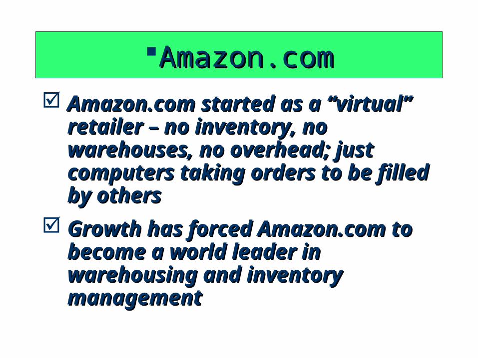
Amazon.comAmazon.com Amazon.com started as a “virtual” Amazon.com started as a “virtual”
retailer – no inventory, no retailer – no inventory, no warehouses, no overhead; just warehouses, no overhead; just computers taking orders to be filled computers taking orders to be filled by othersby others
Growth has forced Amazon.com to Growth has forced Amazon.com to become a world leader in become a world leader in warehousing and inventory warehousing and inventory managementmanagement

What Is Inventory?What Is Inventory?
Stock of items kept to meet future demand
Working Capital Def. - A physical resource that a firm Def. - A physical resource that a firm
holds in stock with the intent of selling it holds in stock with the intent of selling it or transforming it into a more valuable or transforming it into a more valuable state.state.

Inventory by Nature of MaterialInventory by Nature of Material
Raw MaterialsRaw Materials Works-in-Process Works-in-Process Finished GoodsFinished Goods Maintenance, Repair and Operating (MRO)Maintenance, Repair and Operating (MRO)

Inventory by Uses of MaterialInventory by Uses of Material
Transaction Inventory Speculative Inventory Precautionary Inventory

Functional Classification Of Functional Classification Of InventoryInventory
Based on utility, all inventory can be in one or Based on utility, all inventory can be in one or more of the following categoriesmore of the following categories Working stockWorking stock Safety stockSafety stock Anticipation stockAnticipation stock Pipeline stockPipeline stock Decoupling stockDecoupling stock Psychic stockPsychic stock

Cost of InventoryCost of Inventory

1.Ordering /Procurement cost1.Ordering /Procurement cost
Cost of replenishing inventoryCost of replenishing inventory Order processingOrder processing ShippingShipping HandlingHandling

2.Carrying Costs2.Carrying Costs
Cost of holding an item in inventoryCost of holding an item in inventory Working Capital (opportunity) costsWorking Capital (opportunity) costs Inventory risk costs( spoilage, breakage, Inventory risk costs( spoilage, breakage,
detoriation ,obsolescence)detoriation ,obsolescence) Space costsSpace costs Inventory service costsInventory service costs Insurance & TaxesInsurance & Taxes

3.Out-of-Stock Costs/Shortage Cost3.Out-of-Stock Costs/Shortage Cost
Lost sales costLost sales cost Back-order costBack-order cost

Inventory ManagementInventory Management If company holds too little InventoryIf company holds too little Inventory
too frequent orderingtoo frequent ordering
loss of quantity discountloss of quantity discount
higher transportation chargeshigher transportation charges
likely shortage in futurelikely shortage in future
If company holds too much InventoryIf company holds too much Inventory
carrying/holding chargescarrying/holding charges
storagestorage
obsolescence, depreciationobsolescence, depreciation
Involvement of working capitalInvolvement of working capital

Objectives of Inventory ManagementObjectives of Inventory Management
1) Maximize the level of customer service 1) Maximize the level of customer service by avoiding under stocking.(How much to by avoiding under stocking.(How much to order?)order?)
2) Promote efficiency in production and 2) Promote efficiency in production and purchasing by minimizing the cost of purchasing by minimizing the cost of providing an adequate level of customer providing an adequate level of customer service.(When to order?)service.(When to order?)
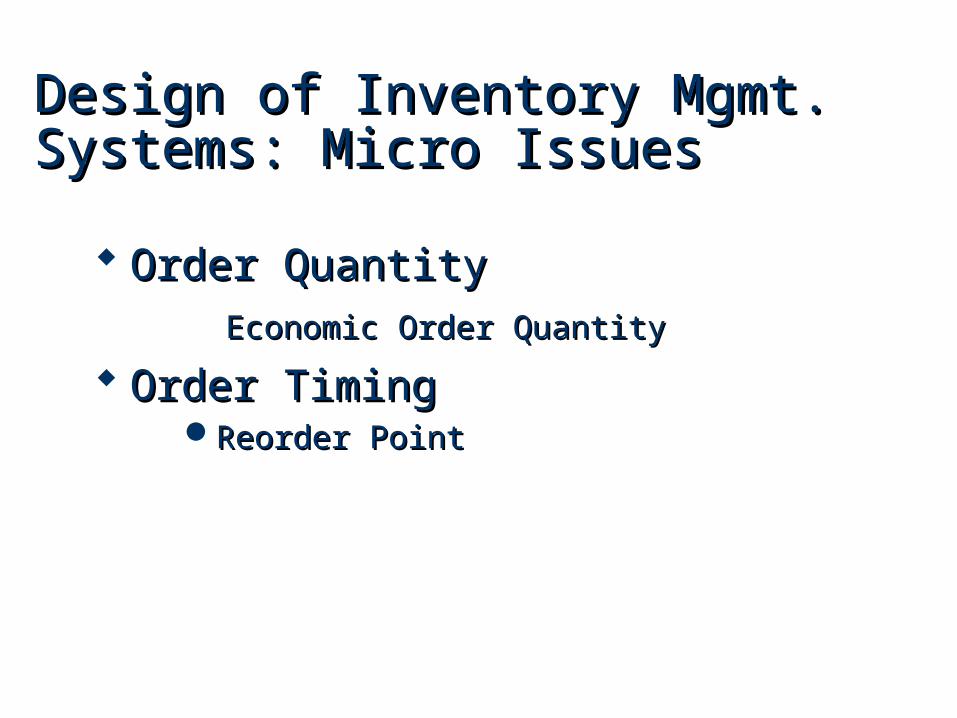
Design of Inventory Mgmt. Systems: Design of Inventory Mgmt. Systems: Micro IssuesMicro Issues
Order QuantityOrder Quantity
Economic Order QuantityEconomic Order Quantity
Order TimingOrder TimingReorder PointReorder Point

Inventory SystemsInventory Systems Single-Period Inventory ModelSingle-Period Inventory Model
One time purchasing decision (Example: One time purchasing decision (Example: vendor selling t-shirts at a football game)vendor selling t-shirts at a football game)
Seeks to balance the costs of inventory Seeks to balance the costs of inventory overstock and under stockoverstock and under stock
Multi-Period Inventory ModelsMulti-Period Inventory Models Fixed-Order Quantity ModelsFixed-Order Quantity Models
Event triggered (Example: running out of Event triggered (Example: running out of stock)stock)

Single-Period Inventory ModelSingle-Period Inventory Model
uo
u
CC
CP
sold be unit will y that theProbabilit
estimatedunder demand ofunit per Cost C
estimatedover demand ofunit per Cost C
:Where
u
o
P
This model states that we This model states that we should continue to should continue to increase the size of the increase the size of the inventory so long as the inventory so long as the probability of selling the probability of selling the last unit added is equal to last unit added is equal to or greater than the ratio or greater than the ratio of: Cu/Co+Cuof: Cu/Co+Cu
This model states that we This model states that we should continue to should continue to increase the size of the increase the size of the inventory so long as the inventory so long as the probability of selling the probability of selling the last unit added is equal to last unit added is equal to or greater than the ratio or greater than the ratio of: Cu/Co+Cuof: Cu/Co+Cu

Single Period Model ExampleSingle Period Model Example Our college basketball team is playing in a Our college basketball team is playing in a
tournament game this weekend. Based on our tournament game this weekend. Based on our past experience we sell on average 2,400 shirts past experience we sell on average 2,400 shirts with a standard deviation of 350. We make with a standard deviation of 350. We make Rs100 on every shirt we sell at the game, but Rs100 on every shirt we sell at the game, but lose Rs50 on every shirt not sold. How many lose Rs50 on every shirt not sold. How many shirts should we make for the game?shirts should we make for the game?
CCuu = = Rs100 and Rs100 and CCoo = Rs50; = Rs50; PP ≤ ≤ 100 / (100 + 50) = .667 100 / (100 + 50) = .667
ZZ.667.667 = .432 (use NORMSDIST(.667) or Appendix E) = .432 (use NORMSDIST(.667) or Appendix E)
therefore we need 2,400 + .432(350) = 2,551 shirtstherefore we need 2,400 + .432(350) = 2,551 shirts
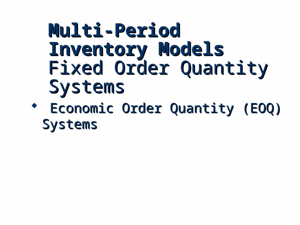
Multi-Period Inventory Multi-Period Inventory ModelsModelsFixed Order Quantity SystemsFixed Order Quantity Systems
Economic Order Quantity (EOQ) Economic Order Quantity (EOQ) SystemsSystems

Behavior of EOQ SystemsBehavior of EOQ Systems As demand for the inventoried item occurs, As demand for the inventoried item occurs,
the inventory level dropsthe inventory level drops When the inventory level drops to a critical When the inventory level drops to a critical
point, the order point, the ordering process is point, the order point, the ordering process is triggered triggered
The amount ordered each time an order is The amount ordered each time an order is placed is fixed or constantplaced is fixed or constant
When the ordered quantity is received, the When the ordered quantity is received, the inventory level increasesinventory level increases

Basic Fixed-Order Quantity Model Basic Fixed-Order Quantity Model and Reorder Point Behaviorand Reorder Point Behavior
R = Reorder pointR = Reorder pointQ = Economic order quantityQ = Economic order quantityL = Lead timeL = Lead time
LL LL
QQ QQQQ
RR
TimeTime
NumberNumberof unitsof unitson handon hand
1. You receive an order quantity 1. You receive an order quantity QQ..
2. Your start using 2. Your start using
them up over timethem up over time.. 33. . When you reach down to a level When you reach down to a level of inventory of R, you place your next of inventory of R, you place your next
Q sized orderQ sized order..
4. The cycle then repeats4. The cycle then repeats..

Inventory Order CycleInventory Order Cycle
Demand Demand raterate
TimeTimeLead Lead timetime
Lead Lead timetime
Order Order placedplaced
Order Order placedplaced
Order Order receiptreceipt
Order Order receiptreceipt
Inven
tory
Inven
tory
Level
Level
Reorder point, Reorder point, RR
Order quantity, Order quantity, QQ
00
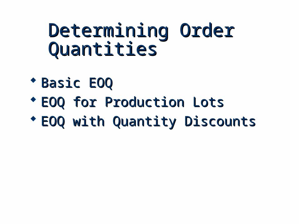
Determining Order QuantitiesDetermining Order Quantities
Basic EOQBasic EOQ EOQ for Production LotsEOQ for Production Lots EOQ with Quantity DiscountsEOQ with Quantity Discounts
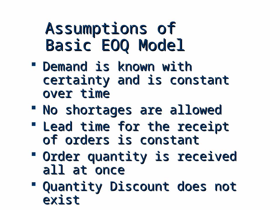
Assumptions of Basic Assumptions of Basic EOQ ModelEOQ Model
Demand is known with certainty and Demand is known with certainty and is constant over timeis constant over time
No shortages are allowedNo shortages are allowed Lead time for the receipt of orders is Lead time for the receipt of orders is
constantconstant Order quantity is received all at onceOrder quantity is received all at once Quantity Discount does not existQuantity Discount does not exist Average Invenory is half of total Average Invenory is half of total
inventoryinventory

EOQ Cost ModelEOQ Cost Model
CCoo - cost of placing order - cost of placing order DD - annual demand - annual demand
CCcc - annual per-unit carrying cost - annual per-unit carrying cost QQ - order quantity - order quantity
Annual ordering cost =Annual ordering cost =CCooDD
Annual carrying cost =Annual carrying cost =CCccQQ
22
Total cost = +Total cost = +CCooDD
CCccQQ
22

EOQ Cost ModelEOQ Cost Model
Proving equality of costs at optimal point
=CoD
Q
CcQ
2
Q2 =2CoD
Cc
Qopt =2CoD
Cc

Cost Minimization GoalCost Minimization Goal
Ordering CostsOrdering Costs
HoldingHoldingCostsCosts
Order Quantity (Q)Order Quantity (Q)
CCOOSSTT
Annual Cost ofAnnual Cost ofItems (DC)Items (DC)
Total CostTotal Cost
QQOPTOPT
By adding the item, holding, and ordering costs By adding the item, holding, and ordering costs together, we determine the total cost curve, which in together, we determine the total cost curve, which in turn is used to find the Qturn is used to find the Qoptopt inventory order point that inventory order point that
minimizes total costsminimizes total costs

Example:Electronic Village stocks and sells a particular brand of personal computer. It costs the store Rs450 each time it places an order with the manufacturer for the personal computers. The annual cost of carrying the PCs in inventory is Rs170. The store manager estimates that annual demand for the PCs will be 1200 units.
Determine the optimal order quantity and the total minimum inventory cost.

Example: Basic EOQExample: Basic EOQ
Zartex Co. produces fertilizer to sell to Zartex Co. produces fertilizer to sell to wholesalers. One raw material – calcium nitrate wholesalers. One raw material – calcium nitrate – is purchased from a nearby supplier at $22.50 – is purchased from a nearby supplier at $22.50 per ton. Zartex estimates it will need 5,750,000 per ton. Zartex estimates it will need 5,750,000 tons of calcium nitrate next year.tons of calcium nitrate next year.
The annual carrying cost for this material is The annual carrying cost for this material is 40% of the acquisition cost, and the ordering 40% of the acquisition cost, and the ordering cost is $595. cost is $595.
a) What is the most economical order a) What is the most economical order quantity?quantity?
b) How many orders will be placed per year?b) How many orders will be placed per year?c) How much time will elapse between orders?c) How much time will elapse between orders?

Example 10.2 Example 10.2 Electronic Village stocks and sells a particular Electronic Village stocks and sells a particular
brand of personal computer. It costs the store brand of personal computer. It costs the store Rs450 each time it places an order with the Rs450 each time it places an order with the manufacturer for the personal computers. The manufacturer for the personal computers. The annual cost of carrying the PCs in inventory is annual cost of carrying the PCs in inventory is Rs170. The store Rs170. The store
manager estimates that annual demand for the manager estimates that annual demand for the PCs will be 1200 units. Determine the optimal PCs will be 1200 units. Determine the optimal order quantity and the total minimum inventory order quantity and the total minimum inventory cost. cost.

Reorder PointReorder Point
Quantity to which inventory is allowed to drop Quantity to which inventory is allowed to drop before replenishment order is madebefore replenishment order is made
Need to order EOQ at the Reorder Point:Need to order EOQ at the Reorder Point:
ROP = D X LTROP = D X LT
D = Demand rate per periodD = Demand rate per period
LT = lead time in periodsLT = lead time in periods

ExampleExample
The I-75 Discount Carpet Store is open The I-75 Discount Carpet Store is open 311 days per year. If annual demand is 311 days per year. If annual demand is 10,000 yards of Super Shag Carpet and 10,000 yards of Super Shag Carpet and the lead time to receive an order is 10 the lead time to receive an order is 10 days, determine the reorder point for days, determine the reorder point for carpet. carpet.
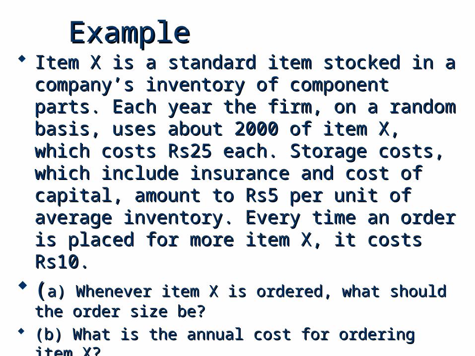
ExampleExample Item X is a standard item stocked in a company’s Item X is a standard item stocked in a company’s
inventory of component parts. Each year the firm, inventory of component parts. Each year the firm, on a random basis, uses about 2000 of item X, on a random basis, uses about 2000 of item X, which costs Rs25 each. Storage costs, which which costs Rs25 each. Storage costs, which include insurance and cost of capital, amount to include insurance and cost of capital, amount to Rs5 per unit of average inventory. Every time an Rs5 per unit of average inventory. Every time an order is placed for more item X, it costs Rs10. order is placed for more item X, it costs Rs10.
((a) Whenever item X is ordered, what should the order size a) Whenever item X is ordered, what should the order size be? be?
(b) What is the annual cost for ordering item X? (b) What is the annual cost for ordering item X? (c) What is the annual cost for storing item X? (c) What is the annual cost for storing item X?

Production Quantity Model(EOQ for lot) An inventory system in which an order is received
gradually, as inventory is simultaneously being depleted
Non-instantaneous receipt model assumption that Q is received all at once is relaxed
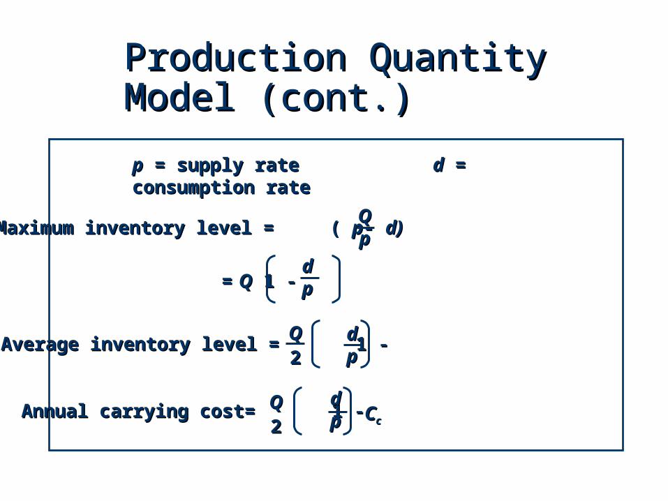
p - daily rate at which an order is received over time, production rate
d - daily rate at which inventory is demanded

Assumptions of Production Quantity ModelAssumptions of Production Quantity Model
Demand is known with certainty and is constant Demand is known with certainty and is constant over timeover time
No safety stockNo safety stock No shortages are allowedNo shortages are allowed Lead time for the receipt of orders is constantLead time for the receipt of orders is constant Goods are supplied (p)at and consumed (d)at Goods are supplied (p)at and consumed (d)at
uniform rate,uniform rate, Supply rate is greater than usage rate.Supply rate is greater than usage rate. Quantity Discount does not existQuantity Discount does not exist
Production Quantity Model Production Quantity Model (cont.)(cont.)
pp = supply rate = supply rate dd = consumption rate = consumption rate
Maximum inventory level =Maximum inventory level = ( ( pp- - d)d)
== QQ 1 - 1 -
QQpp
ddpp
Average inventory level = Average inventory level = 1 - 1 -QQ22
ddpp
Annual carrying cost= Annual carrying cost= 1 - 1 -QQ22
ddpp CCcc
Production Quantity Model Production Quantity Model (cont.)(cont.)
pp = supply rate = supply rate dd = consumption rate = consumption rate
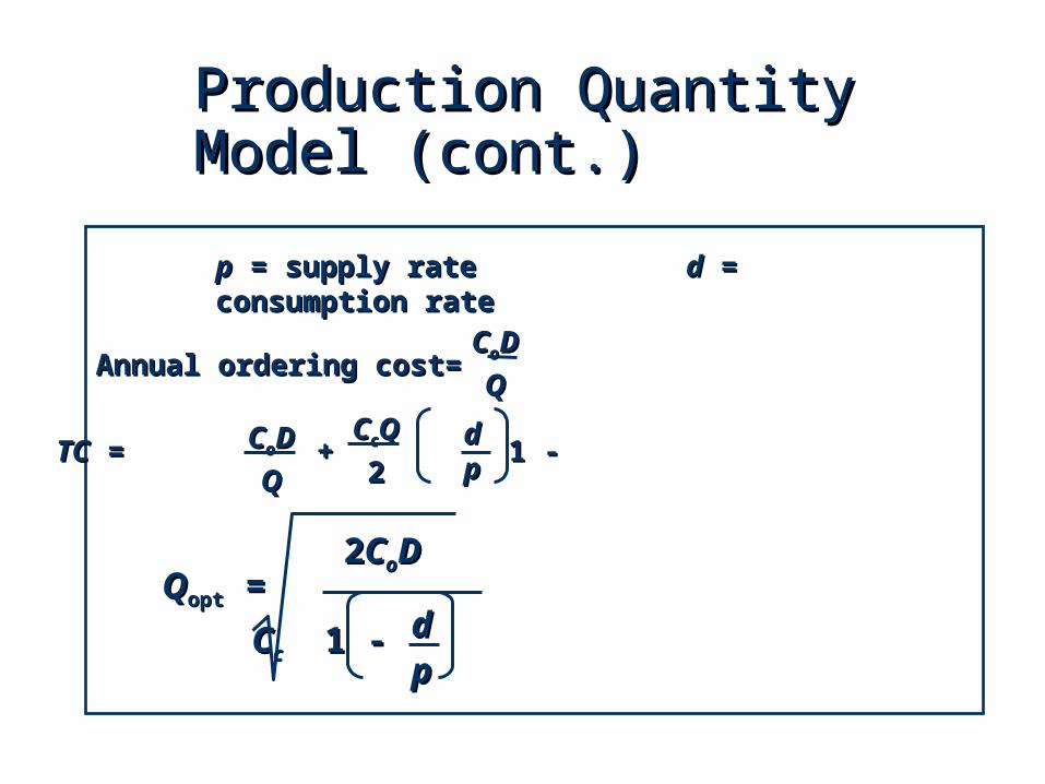
Annual ordering cost=Annual ordering cost=
TCTC = + 1 - = + 1 - ddpp
CCooDD
CCccQQ
22
QQoptopt = =22CCooDD
CCcc 1 - 1 - ddpp
CCooDD

Production Quantity Model Production Quantity Model (cont.)(cont.)
QQ(1-(1-d/pd/p))
InventoryInventorylevellevel
(1-(1-d/pd/p))QQ22
TimeTime00
OrderOrderreceipt periodreceipt period
BeginBeginorderorder
receiptreceipt
EndEndorderorder
receiptreceipt
MaximumMaximuminventory inventory levellevel
AverageAverageinventory inventory levellevel
(p-(p-dd))
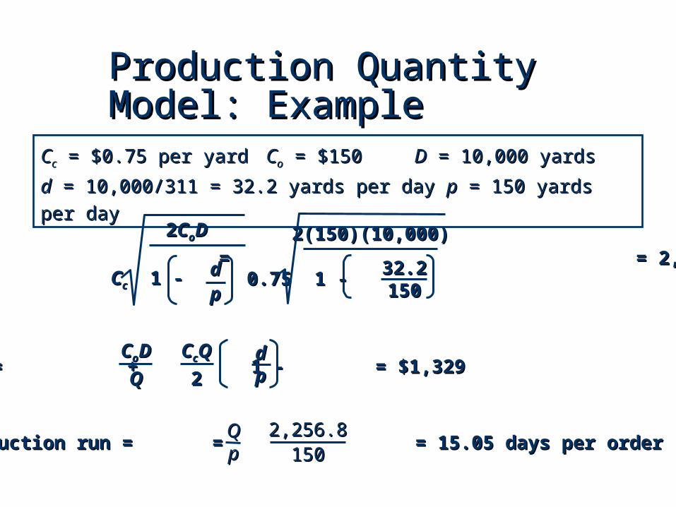
Production Quantity Model: Production Quantity Model: ExampleExample
CCcc = $0.75 per yard = $0.75 per yard CCoo = $150 = $150 DD = 10,000 yards = 10,000 yards
dd = 10,000/311 = 32.2 yards per day = 10,000/311 = 32.2 yards per day pp = 150 yards per day = 150 yards per day
QQoptopt = = = 2,256.8 yards = = = 2,256.8 yards
22CCooDD
CCcc 1 - 1 - ddpp
2(150)(10,000)2(150)(10,000)
0.75 1 - 0.75 1 - 32.232.2150150
TCTC = + 1 - = $1,329 = + 1 - = $1,329ddpp
CCooDD
CCccQQ
22
Production run = = = 15.05 days per orderProduction run = = = 15.05 days per orderQQpp
2,256.82,256.8150150

Production Quantity Model: Production Quantity Model: Example (cont.)Example (cont.)
Number of production runs = = = 4.43 runs/yearDQ
10,0002,256.8
Maximum inventory level = Q 1 - = 2,256.8 1 -
= 1,772 yards
dp
32.2150
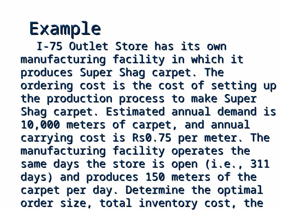
ExampleExample I-75 Outlet Store has its own manufacturing facility in I-75 Outlet Store has its own manufacturing facility in
which it produces Super Shag carpet. The ordering which it produces Super Shag carpet. The ordering cost is the cost of setting up the production process cost is the cost of setting up the production process to make Super Shag carpet. Estimated annual to make Super Shag carpet. Estimated annual demand is 10,000 meters of carpet, and annual demand is 10,000 meters of carpet, and annual carrying cost is Rs0.75 per meter. The manufacturing carrying cost is Rs0.75 per meter. The manufacturing facility operates the same days the store is open facility operates the same days the store is open (i.e., 311 days) and produces 150 meters of the (i.e., 311 days) and produces 150 meters of the carpet per day. Determine the optimal order size, carpet per day. Determine the optimal order size, total inventory cost, the length of time to receive an total inventory cost, the length of time to receive an order, the number of orders per year, and the order, the number of orders per year, and the maximum inventory level. maximum inventory level.

Example: EOQ for Production LotsExample: EOQ for Production Lots
Highland Electric Co. buys coal from Highland Electric Co. buys coal from Cedar Creek Coal Co. to generate electricity. Cedar Creek Coal Co. to generate electricity. CCCC can supply coal at the rate of 3,500 CCCC can supply coal at the rate of 3,500 tons per day for $10.50 per ton. HEC uses the tons per day for $10.50 per ton. HEC uses the coal at a rate of 800 tons per day and operates coal at a rate of 800 tons per day and operates 365 days per year.HEC’s annual carrying cost 365 days per year.HEC’s annual carrying cost for coal is 20% of the acquisition cost, and the for coal is 20% of the acquisition cost, and the ordering cost is $5,000.ordering cost is $5,000.
a) a) What is the economical production lot size?What is the economical production lot size?
b) What is HEC’s maximum inventory level for coalb) What is HEC’s maximum inventory level for coal??
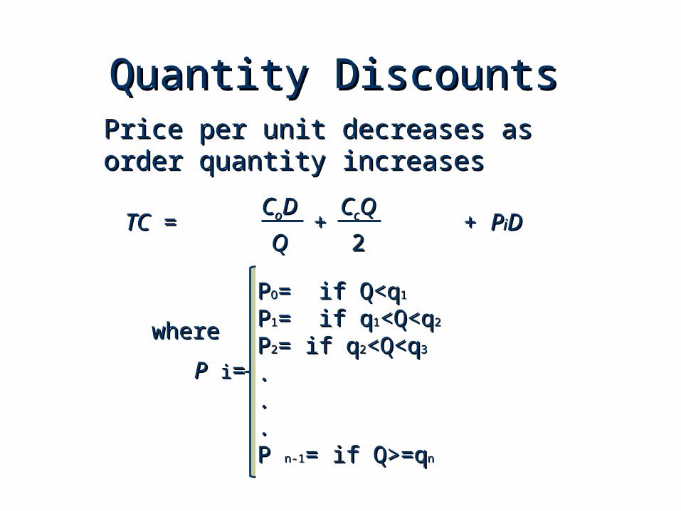
Quantity DiscountsQuantity DiscountsPrice per unit decreases as order Price per unit decreases as order quantity increasesquantity increases
TCTC = + + = + + PPiiDDCCooDD
CCccQQ
22
wherewhere
PP ii==
PPOO= if Q<q= if Q<q11
PP11= if q= if q11<Q<q<Q<q22
PP22= if q= if q22<Q<q<Q<q33
..
..
..P P n-1n-1= if Q>=q= if Q>=qnn

Quantity DiscountsQuantity DiscountsPrice per unit decreases as order Price per unit decreases as order quantity increasesquantity increases
wherewhere
PP ii==
PPOO= if Q<q= if Q<q11
PP11= if q= if q11<Q<q<Q<q22
PP22= if q= if q22<Q<q<Q<q33
..
..
..P P n-1n-1= if Q>=q= if Q>=qnn
22CCooDD
CCcc
QQoptmoptm==
WhereWhere
CCcc= I *P= I *Pii
I =carrying cost %I =carrying cost %

Quantity Discount Model (cont.)Quantity Discount Model (cont.)
QQoptopt
Carrying cost Carrying cost
Ordering cost Ordering cost
Inventory cost Inventory cost ($)($)
QQ((dd1 1 ) = 100) = 100 QQ((dd2 2 ) = 200) = 200
TC TC ((dd2 2 = $6 ) = $6 )
TCTC ( (dd1 1 = $8 )= $8 )
TC TC = ($10 )= ($10 ) ORDER SIZE PRICE
0 - 99 $10
100 – 199 8 (d1)
200+ 6 (d2)

Price-Break Example Problem Data Price-Break Example Problem Data (Part 1)(Part 1)
A company has a chance to reduce their inventory A company has a chance to reduce their inventory ordering costs by placing larger quantity orders using ordering costs by placing larger quantity orders using the price-break order quantity schedule below. What the price-break order quantity schedule below. What should their optimal order quantity be if this company should their optimal order quantity be if this company purchases this single inventory item with an e-mail purchases this single inventory item with an e-mail ordering cost of Rs4, a carrying cost rate of 2% of the ordering cost of Rs4, a carrying cost rate of 2% of the inventory cost of the item, and an annual demand of inventory cost of the item, and an annual demand of 10,000 units?10,000 units?
A company has a chance to reduce their inventory A company has a chance to reduce their inventory ordering costs by placing larger quantity orders using ordering costs by placing larger quantity orders using the price-break order quantity schedule below. What the price-break order quantity schedule below. What should their optimal order quantity be if this company should their optimal order quantity be if this company purchases this single inventory item with an e-mail purchases this single inventory item with an e-mail ordering cost of Rs4, a carrying cost rate of 2% of the ordering cost of Rs4, a carrying cost rate of 2% of the inventory cost of the item, and an annual demand of inventory cost of the item, and an annual demand of 10,000 units?10,000 units?
Order Quantity(units)Order Quantity(units)Price/unit(Rs)Price/unit(Rs) 0 to 2,499 0 to 2,499 Rs1.20Rs1.20 2,500 to 3,999 1.002,500 to 3,999 1.00 4,000 or more .984,000 or more .98

Price-Break Example Solution (Part 2)Price-Break Example Solution (Part 2)
units 1,826 = 0.02(1.20)
4)2(10,000)( =
C
2DC = Q
cOPT
0
Annual Demand (D)= 10,000 unitsAnnual Demand (D)= 10,000 unitsCost to place an order (S)= Rs4Cost to place an order (S)= Rs4
First, plug data into formula for each price-break value of “C”First, plug data into formula for each price-break value of “C”
units 2,000 = 0.02(1.00)
4)2(10,000)( =
C
2DC = Q
c
o
OPT
units 2,020 = 0.02(0.98)
4)2(10,000)( =
C
2DC = Q
c
o
OPT
Carrying cost % of total cost (i)= Carrying cost % of total cost (i)= 2%2%Cost per unit (C) = $1.20, $1.00, $0.98Cost per unit (C) = $1.20, $1.00, $0.98
Interval from 0 to 2499, Interval from 0 to 2499, the Qthe Qoptopt value is feasible value is feasible
Interval from 2500-3999, the Interval from 2500-3999, the QQoptopt value is not feasible value is not feasible
Interval from 4000 & more, Interval from 4000 & more, the Qthe Qoptopt value is not feasible value is not feasible
Next, determine if the computed QNext, determine if the computed Qoptopt values are feasible or not values are feasible or not
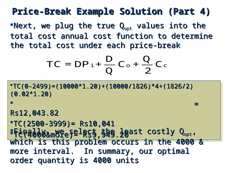
Price-Break Example Solution (Part 4)Price-Break Example Solution (Part 4)
coi C 2
Q + C
Q
D + DP = TC
Next, we plug the true QNext, we plug the true Qoptopt values into the total cost annual values into the total cost annual
cost function to determine the total cost under each price-cost function to determine the total cost under each price-breakbreak
TC(0-2499)=(10000*1.20)+(10000/1826)*4+(1826/2)(0.02*1.20)TC(0-2499)=(10000*1.20)+(10000/1826)*4+(1826/2)(0.02*1.20)
= Rs12,043.82= Rs12,043.82TC(2500-3999)= Rs10,041TC(2500-3999)= Rs10,041TC(4000&more)= Rs9,949.20TC(4000&more)= Rs9,949.20
TC(0-2499)=(10000*1.20)+(10000/1826)*4+(1826/2)(0.02*1.20)TC(0-2499)=(10000*1.20)+(10000/1826)*4+(1826/2)(0.02*1.20)
= Rs12,043.82= Rs12,043.82TC(2500-3999)= Rs10,041TC(2500-3999)= Rs10,041TC(4000&more)= Rs9,949.20TC(4000&more)= Rs9,949.20
Finally, we select the least costly QFinally, we select the least costly Qoptopt, which is this problem , which is this problem
occurs in the 4000 & more interval. In summary, our optimal occurs in the 4000 & more interval. In summary, our optimal order quantity is 4000 unitsorder quantity is 4000 units
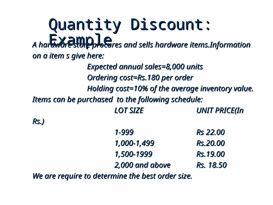
Quantity Discount: ExampleQuantity Discount: ExampleA hardware store procures and sells hardware items.Information A hardware store procures and sells hardware items.Information
on a item s give here:on a item s give here:
Expected annual sales=8,000 unitsExpected annual sales=8,000 units
Ordering cost=Rs.180 per orderOrdering cost=Rs.180 per order
Holding cost=10% of the average inventory value.Holding cost=10% of the average inventory value.
Items can be purchased to the following schedule:Items can be purchased to the following schedule:
LOT SIZELOT SIZE UNIT PRICE(In UNIT PRICE(In
Rs.)Rs.)
1-9991-999 Rs 22.00Rs 22.00
1,000-1,4991,000-1,499 Rs.20.00Rs.20.00
1,500-19991,500-1999 Rs.19.00Rs.19.00
2,000 and above2,000 and above Rs. 18.50Rs. 18.50
We are require to determine the best order size.We are require to determine the best order size.