INTERVAL MEASUREMENT OF SlJBJECTIVE MAGNITUDES
WITH SlJBLIMINAL D:tF'FERENCES
BY
MURIEL WOOD GERLACH
TECHNICAL REPORT NO. 7
APRIL 17, 1957
PREPARED UNDER CONTRACT Nonr 225(17)
(NR 171-034)
FOR
OFFICE OF NAVAL RESEARCH
REPRODUCTION IN WHOLE OR IN PART IS
PERMITTED FOR ANY PURPOSE OF
THE UNITED STATES GOVERNMENT
BEHAVIORAL SCIENCES DIVISION
APPLIED MATHEMATICS AND STATISTICS LABORATORY
STANFORD UNIVERSITY
STANFORD, CAL:tF'ORNIA

Il
f

INTERVAL MEASUREMENT OF SUBJECTIVE MAGNITUDES
WITH SUBLIMINAL DIFFERENCES
by
Muriel Wood Gerlach
I. INTRODUCTION: THE PROBLEM OF PSYCHOLOGICAL MEASUREMENT
There are many aspects of things and events which are best discrimi
nated, if at all, by the direct responses of living beings, human or
animal. For example, while the objective weight of an object may be
determined by placing it on an equal arm balance, the determination of
its felt weight to an individual requires his own response to hefting
the object. The problem of subjective (psychological, sensory) measure
ment arises when we are concerned with discriminating such aspects of
things as their felt weight, seen color, perceived tone, or psychological
value, (in contrast to their objective weight, luminosity, physical
acoustics, or monetary worth). The discrimination in question is obvi
ously a matter of the sensory responses of living observers, it is not
based on the mechanical or electrical variations of physical instruments
(scales, dials, meters). Is such discrimination capable of yielding
quantitative orders? Can the subjectively discriminated aspects of
things be systematically arranged to form consistent arrays? In brief,
is psychological measurement possible? The purpose of our introduction
is to discuss some of the answers which have been given to this question
and to indicate the relevance of our theory to the iiproblemii of subjec-
tive measurement as we see it.
-2-
We shall consider three types of answers to the question. The first two
are categorical in character, the third is hypothetical or conditional. Onthe
first view, presented in uncompromising fashion by several members of the British
"committee appointed to consider and report upon the possibility of quantitative
estimates of sensory events, il the answer is a categorical negative 0
The members of this committee suggest as one reason for their skepticism
that HfundamentalH measurement is impossible in psychology, asserting that the
measurement of psychological magnitudes depends on the prior measurement of
physical magnitudes. Since, according to these scientists, Hfundamental" measure
ment is the only type of measurement worthy of the name, they argue that psycho
logical measurement, in any true sense of the word, is impossible. Their point
seems to be that when, for example, Stevens and Volkmann construct a pitch func
tion (Stevens and Volkmann [23]), pitch, a psychological attribute, scaled in
subjective units (mels), is plotted against frequency, a physical attribute
measured in physical units. Hence, they say, the measurement of pitch depends
on the prior measurement of frequency. Similarly, the measurement of any other
psychological magnitude depends on prior physical measurement of the correlated
stimulus, and is therefore not fundamental.
This argument has been convincingly answered by Reese (Reese, [18], pp. 44
46) who reminds us that subjective measurement has been effected where the
stimulus correlate is unknown (as in the measurement of I.Q.); or where no
independent physical measurement exists (as in the scaling of attitudes); or
where the stimulus correlate is exceedingly complex, i.e., the psychological
attribute in question is not a perfectly monotonic or linear or single-valued
function of a single physical dimension (as in the case of the pleasingness of

o
-3-
handwriting which is no doubt correlated with the size, shape, etc., of
the physical inscriptions but in an obscure and complicated manner).
Reese goes on to point out that where the stimulus correlate can be
identified and measured, the use of 'physical measures in constructing
psychological scales may be regarded as incidental. Despite classical
psychophysical procedures, there is nothing about subjective measure
ment which essentially requires the direct quantitative use of an
underlying physical continuum. Some method for identifying the subjec
tive phenomena under investigation is required; (for example, the
different identifiable pitches must somehow be indicated); where a
physical correlate is known, it is convenient to identify a psychological
element by reference to the physical stimulus with which it is associated;
where the correlated physical magnitude is measurable, it is helpful for
the investigation of functional relationships to plot the subjective
magnitudes against the physical magnitudes arranged in their order as
measured, rather than plotting the subjective magnitudes against the
physical magnitudes considered merely as identification tags for the
former, and therefore random in their position along the abscissa. But
the fact remains that any method of identifying the subjective phenomena
in question will do. Reese remarks that arbitrary marks on the dial of
the reproducing instrument will serve the purpose; Goodman suggests
identifications with no physical connotations whatsoever: A particular
color may be singled out as lithe color of the left-hand one of the two
round patches now near the center of my visualfield~i (Goodman [9],
p. 226.)

-4-
To Reese's cogent refutations of the argument that psychological measure-
ment cannot be regarded as "fundamental" measurement and therefore does not
really constitute measurement, we should like to add a further consideration,
It is not clear to us that the traditional distinction between "fundamentall'
and "derived" measurement can be upheld. The orthodox view is that "derived"
measurement is dependent on prior measurement of some sort where "fundamental lV
measurement is independent in this respect, (Hempel [10], pp. 62-74,) But,
just as defined notions are theoretically eliminable in favor of the primitive
notions by which they are defined, so too the prior measurement supposedly
assumed in "derivedH measurement is eliminable in favor of the non-quantitative
concepts from which it was originally constructed, The distinction between
:fundamental and derived measurement thus appears to be dubious; and in so far
as the case against psychological measurement rests on this dichotomy, it is
lacking in force.
More compelling arguments have been advanced against the possibility of
quantifying subjective phenomena. These arguments often take the general form
of asserting that it is impossible to find empirical operations in the sub-
jective realm which will correspond to the numerical operations of measurement
(addition, subtraction, division, multiplication). It has been said, for
example, that to assign numbers to sensations requires that one sensation be
half or twice another sensation which is absurd since sensations are simple,
unanalyzable, unitary; they are not the sort of things that can be divided
and fragmented, This sort of objection is clearly naive; for to characterize
a sensation x as twice as intense as another sensation y is not to say
that sensation y is half of sensation x in the same way that half an apple
is half of a whole apple, (Stevens' choice of such names as lifractionation"
•f

-5-
or "bisection" for his methods of sensory scaling seems, therefore, excep
tionally unfortunate.) Actually no operation of sensory fragmentation or
division is required. The numerical statement might mean that sensation y
if added to itself in an appropriate way would produce sensation x. If
this interpretation were chosen, clearly an operation for sensory iladditions"
would be required. Such phenomena as the monaural-binaural phenomenon in
auditory sensation provide evidence that such a requirement can be met in
some sensory domains. For there is some evidence that a sound y intro
duced into one ear may be "added" to itself by being introduced into both
ears to produce a sound x which is subjectively twice as loud as y. In
fact, Campbell himself has admitted that the monaural-binaural method of
scaling satisfies the requirement for a subjective operation of lIaddition.t!
An even more natural interpretation of the characterization of a sensation
as "half" of another sensation than the 'iadditive," one just discussed is
suggested by Wiener. He writes that lisuch a proposition as IX is twice
as intense as y' is simply a paraphrase for some such statement as "the
interval of intensity between x and y equals that between y and some
sensation of zero intensity i • Ii (Wiener [29), p. 1830) According to this
view, the half judgment requires neither the fragmentation nor the liaddi
tiont! of sensation, but only the equation of sense-distances and a natural
zero. It is usually granted that sense-distances are introspectively com
parable; and, recently, members of the Stanford group have shown that
behavioristic interpretations can be provided for the notion of equal sense
distances 0 (Davidson and Suppes [6] ,pp 0 12-16, Suppes and Winet [24], pp. 259.f6lo)
It seems probable that the mathematical notions essentially required
for measurement are, after all, amenable to psychological interpretation.
But the critics of sensory measurement may raise a more serious objection.
-6-
They may protest that the subjective operations specified as empirical inter
pretationsfor the formal notions are incapable of satisfying the logical
criteria which must be met if measurement is to result. To take a single
example especially pertinent to this dissertation, the notion of equal sense
distances has been criticized on the grounds that sensory equality does not
have the properties of mathematical equality. Equality of arithmetical dif
ference is reflexive, sYmmetrical and transitive; but a sensory difference
may be equated with a second, the second with a third, and yet the third and
the first will seem unequal. If transitivity does not hold for the equation
of sense~differences, then we are not justified in passing from an adequate
formal scheme for measurement where equality is assumed to be transitive, to
the claim that we have achieved subjective measurement merely by providing
an empirical realization in the psychological realm for the formal notion of
equality. It is true that unless we can find suitable interpretations for
our formal notions which will satisfy the requisite logical criteria, we can
not pretend to have measurement. But notice that we have slipped from an
unconditional denial of the possibility of psychological measurement, to a
position whereby ingenuity, by modifying either the supposed formal require
ments, or alternatively, by discovering new empirical operations capable of
satisfying the logical criteria in question, may achieve the desired result
and fimagnitudes not now measurable will turn out to be measurable. 1i (Reese
[18], p. 16.)
At any rate, the arguments we have examined rejecting subjective measure
ment as an impossibility seem all to have an objectionable ~ priori character
about them. It is asserted as an unquestionable fact that we cannot find

-7-
psychological operations which will fulfill the formal criteria of measure
ment. Meanwhile, however, reputable psychologists, economists and other
scientists working in the realm of human or animal behavior are unabashedly
assigning numbers to their data, and manipulating them according to general
mathematical techniques. Economists have for a long time plotted utility
curves, and spoken of measurable utility; more recently, they have attempted
to assess numerically such notions as subjective probability; psychophys
icists have constructed scales for such subjective magnitudes as loudness,
pitch, and visual numerousness; psychologists have developed methods for
scaling personality traits, intelligence, and even the quality of hand
writing or artistic compositions. To such scientists, the question whether
psychological measurement is possible must seem an anachronism. To them,
psychological measurement is not a remote possibility, it is an accomplished
fact.

-8-

-9-
Hence, since our numbering should reflect our preferential ranking, the
numbers assigned to a and to c must differ; but since a and bare
indifferent, b must have the same number as a, which requires, since
band c are indifferent, that c have the same number as a. Clearly,
a contradiction ensueso Nor does this difficulty depend in any way upon
the notion of combinations of goods central to indifference curve analysis.
The graphical method of discussing indifference curves obscures this point,
and one might think that indifference-classes arise only in the case where
we are concerned with vector quantities. Actually, the notion of an
indifference-class arises whenever elements can fall into the same posi
tion ina ranking, whether these elements be similarly ranked complexes
of objects combined in differing proportions or absolutely simple elements,
positionally indistinguishable one from the other (as, for example, when
horses are tied in a race). Armstrong's objection is, therefore, telling;
and unless we are willing to assert that subliminal difference do not
exist, or that elements can never be positionally indistinguishable, we
must meet the problem for measurement raised by indifference-classes. It
is a major purpose of this dissertation to propose a non-contradictory
method for the assignment of numbers to a set of elements, without deny
ing that two or more elements may stand in a relation of indifference to
one another, or that imperceptible differences may exist.
A widely used scheme for subjective measurement seems to overcome
the difficulty just outlined by actually basing the assignment of numbers
upon the troublesome subliminal differences which exist in any sensory
field. Essentially the type of measurement used by Fechner, this method

-10-
can be characterized as the summation of jnds (just noticeable differences
between stimuli). If a stimulus has assigned to ita certain numerical value
representing its subjective magnitude, then the value assigned to any other
stimulus is determined by counting up the number of jnds between the two
stimuli, due account being taken of directional order: thus if m is the
number assigned to the first stimulus, and n is the number of just notice
able sensory steps in an ascending direction between the first and the second
stimulus, then the number p assigned to the latter must equal m+n. In
other words, the jnd is taken as the unit of subjective distance.
Subjective measurement by the counting of jnds is open to two objec
tions. Most obviously, it is incomplete. What number representing sensory
magnitude is to be assigned to a stimulus lying between two stimuli just
noticeably different from one another? It may be thought that there is no
problem here, for, since we are constructing a sensory scale, we are not
required to number every physical stimulus, but only to arrange and classify
our sensory experiences. But it is not clear that sensory experiences can
be identified except in terms of the stimulating agents (this point will be
discussed at length in section 2); and to us the only reasonable way of
making sense of the notion of sensory orders to to regard such orders as the
scaling of physical stimuli according to their subjective effects. It might,
however, seem reasonable to assume that subjectively licorrectif numerical
assignments for a stimulus lying between two just noticeably different
stimuli are easily provided. The intermediate stimulus may with equal
justice be numbered either identically with the lesser or with the greater
of the two just noticeably different stimuli between which it lies, since
it is sensationally equivalent to either. But this apparent identity holds

-11-
only when we make pairwise sensory comparisons of indistinguishable ele
ments. As Goodman puts it, Yialthough two qualia q and r exactly
match, there may be a third quale s that matches one but not the othero
Thus matching qualia are not always identical 0 II We would not wish to
assign the same number to stimuli capable of being sensationally distin
guished in the above manner. Again, we find ourselves confronting the
problem pointed up by Armstrong: the failure of transitivity for sensory
indifference 0
Subjective measurement by counting jnds is most frequently criti
cized in a slightly different way. The point is usually put thus: we
cannot use the jnd as a unit of sensory difference until we have shown
that jnds are "subjectively equal" throughout a sensory domain. Stevens
and Volkmann point out that the method of jnds gives us a type of
measurement only slightly stronger than an ordinal scale; in addition to
ordering a set of items, the counting of jnds gives us a rule for the
assignment of adjacent numerals to the items in the set 0 But it must
not be thought, as Fechner assumed, that this gives us a scale with a
unit. A rule for assigning adjacent numerals to objects or events does
not necessarily create a unit of measurement 0 For one thing, a unit of
measurement must remain invarianto (Stevens and Volkmann [23].) This
objection is, perhaps, not easily grasped. What does it mean to say we
have a constant unit of subjective distance? A natural first attempt at
formulating such a requirement might be to say that given any four elements
x, y, z and w such that x is just noticeably different from y, and
z is just noticeably different from w, then the sense difference between

-12-
x and y seems equal to the sense difference between z and w. At first
glance, this condition seems to hold, since only a ~-noticeable difference
can seem subjectively less than a just noticeable difference, and both
intervals of the type under consideration are just noticeable differences.
But, on the other hand, we note that the condition could not possibly fail
to hold; and, according to the principle that a statement incapable of
empirical refutation is non-empirical, we begin to suspect that our suggested
criterion does not constitute a test for the empirical subjective equality
of jnds at all. We therefore suggest that an indirect test must be used
to determine the equality of subjective magnitude of jnds over a sensory
range. We define an n-chain of jnds to be an ordered n-tuple, <x ,xl" oo,x >,o n
of elements, each item with a higher subscript immediately succeeding the
item with the subscript lesser by 1 by a just noticeable difference. Then we
propose as an indirect criterion for the subjective equality of jnds the
condition that every n-chain of jnds seem equal to every other n-chain of
jnds, where n is any specific integer. (The criterion originally suggested
now turns out to be a special case of this latter criterion, namely, the
case where n~l.) To state the condition differently, we may say that jnds
can be assumed to be subjectively equal over a sensory range only if all
intervals between pairs of stimuli separated by a fixed number of jnds seem
equal. stevens has shown, by some such criterion, that the jnds for loud-
ness are unequal in subjective magnitude; for example, the loudness differ-
ence between a tonal stimulus 10 jnds above threshold seems far greater
than the loudness difference between the threshold tone and the one of 10
jnds (Stevens and Davis [22], pp. 148 ff .. ) liOn the other hand, for pitch,

-13-
. and possibly for saturation, the jnds are subjectively equal; i.e.,
Fechner's postulate is apparently verified. 1i (Stevens [21], p. 36.)
Obviously, the summing of jnds will not give us strong (interval)
measurement in areas where the subjective size of tJ:e jnd varies over
the range to be studied.
Many psychologists have hoped to remedy the defects of the jnd
method of measurement (its unwarranted assumption of equal scale units)
while preserving its goals (the achievement of a stronger than ordinal
type of measurement). The most prominent efforts in this direction have
attempted to develop numerical scales by some variation of the limethod
of equal appearing intervals. 1i According to this method, an arbitrary
interval is selected as a unit; a zero element is chosen; and then the
number assigned to any other element is uniquely determined as the
number of intervals equal to the arbitrary unit lying between the zero
element and the element in question. In application, this method
requires that the observer equate sense-distances; he must somehow
lilay off" subjectively equal units along the sensory scale. The pro
posed advantage of the method is that it achieves interval measurement
(measurement in which the numerical assignment is unique except for the
arbitrary choice of a unit and a zero point), without assuming the sub
jective equality of the scale units. Equal subjective units are
experimentally obtained. We shall argue that the "method of equal
appearing intervals li is no more successful than the jnd method in
generating interval measurement.
Stevens' procedure of "fractionation" provides the most interesting

-14-
example of the use of this method. For purposes of illustration and discus-
sion, we shall consider the "fractionation" procedu:r'e used by Stevens and
Volkmann to construct a pitch scale. (Stevens and Volkmann [23].)
The method of "fractionation" proceeds by two steps. The first step
is to plot a "half-judgment function" as follows. The subject is p:r'esented
with a number of standard stimuli (tones of determinate physical frequency)
selected to cover a wide range of physical magnitudes (all frequencies, say,
between 40 and 12,000 cycles). For each such standard stimulus, the observer
determines the stimulus which appears to him to be half as great. Then the
stimuli (frequencies) judged one-half are plotted against the standard stimuli,
and a curve known as the half-judgment function is fitted to the obtained
points. Such a plot for a group of hypothetical data is shown below.
STIMULUSJUDGEDONE-HALF(physicalunits)
10
98
76
54
32
1
1 2 3 4 5 6 7 8 9 10 11 12 13 14 15 16
STANDARD (physical units)
In this figure, the stimuli judged one-half are plotted, in physical units,

-15-
against their respective standards, also measured in physical units.
The second step of the method is the assignment of numerical values
to the physical stimuli which will represent their relative subjective
magnitudes. First, some arbitrarily selected stimulus is assigned a sub
jective magnitude of zero. In the study of pitch, the frequency associat
ed with the lowest tone on the organ is often taken as the zero element.
Then the number 1 is assigned to another arbitrarily chosen stimulus, a
tone of slightly greater frequency than the zero element. The subjective
distance between these two elements thus becomes the arbitrary unit. For
pitch, the subjective_ unit has been called the 'mel'. Next the half
judgment function is examined to discover the stimulus of which the unity
stimulus was judged half; and to this stimulus, two subjective units are
assigned. Similarly the stimulus now assigned the number two will show
to have been judged half of some other physical stimulus, to which, since
it is presumably twice as great in subjective magnitude as the former,
the number four will be assigned. This process is continued until the
scale is complete, that is, until a curve can be fitted to the points
so obtained in such a way that a subjective magnitude function is plotted
for the whole range of physical stimuli under consideration. (A pitch
scale is complete, when the pitch, in mels, of each audible frequency
is numerically represented.) SUch a plot constructed from the hypo
thetical half-judgment function presented in our earlier figure, is shown
below.

-16-
STIMULUS(subjective units)
20
18
16
14
12
10
8
6
4 /2
2 4 6 8 10 12 14 16
STIMULUS (physical units)
There are several features about the method of "fractionation" which call
for comment. One criticism often raised against it has to do with the half-
judgment required, and it is objected that sensations are indivisible and can-
not be "halved." We have discussed this type of criticism and to a certain
extent, we have shown it to be invalid; to judge that a is half of b
requires merely the ability to equate the sensory distance between a and
b with the sensory distance between a zero element and a. But the objec-
tion nevertheless retains a certain validity. Clearly, the observer's task
is made difficult by the imaginary nature of the zero element. The verbal
instructions given require the observer to set one tone to half the pitch of
another; if this requirement is to be interpreted as the equating of adjacent
sensory intervals, it seems desirable that a so-called "zero" stimulus should
be presented. Where this stimulus is left to the observer's imagination,
unreliable results are bound to occur. Stevens and Volkmann in a fractionation

-17-
experiment in 1940 took this objection into account, by supplying a refer
ence tone which purportedly defined "zero" pitch. However, the assump
tion that any stimulus can be taken as a natural zero, or as defining a
natural zero seems unwarranted for reasons to be presented in Section 4
under the discussion of Axiom Ala. We agree, therefore, with the sug
gested criticism to the extent that if the half-judgment requires a
natural zero, it will not in general be obtainable.
A second criticism has to do with the interpolation reqUired by the
method. Half-judgments are experimentally obtained only for a number of
stimuli; but the subjective magnitude function is a smooth curve; and it
is constructed from a smooth curve fitted to the data provided by the
limited number of half-judgment estimates. It might be thought that
this interpolation is eliminable. But it is easily verified that the
method of construction of the subjective magnitude function is such
that it depends in an essential way on the interpolation of the half
judgment function between the finite number of points for which it is
originally determined; and then, of course, since the magnitude function
is constructed from the half-judgment plot, it is necessarily a smooth
curve. (The situation is similar to the interpolations in the utility
function required for the construction of subjective probability measures
in the Stanford approach.) (DaVidson, Siegel and Suppes [7], pp. 28-29.)
But, it is a violation of the empirical facts to think of a subjective
magnitude scale of the type constructed by Stevens as a continuous func
tion. Stimulus values closer together than one jnd apart ought, on
Stevens' scheme at least, to be mapped into the same sensory magnitude,
thereby resulting in discontinuities. Moreover, the assignment of

-18-
numbers to such intermediate stimuli is not uniquely determined, since a
stimulus may with equal justification be regarded as sensationally equivalent
to either of the two just noticeably different stimuli between which it lies.
Hence, one could argue that Stevens has a method of numerical assignment which
is a relation, but not a function; that is, a given sensation will be assigned
different numbers depending on what pairwise comparisons of stimuli are con
sidered. (We remark that in our system, there is a way of making a sensory
distinction between pairwise indistinguishable stimuli,thus providing justi
fication for a continuous subjective magnitude function.) Of course, in an
area as uncharted as that of psychological magnitudes, interpolation is
especially dangerous while the amount of interpolation required by this method
is excessively high.
A third objection to "fractionationYi is that the formal requirements of
the method are insufficient to guarantee lIintervalYi measurement. To be sure,
the way in which the numerical measures are originally assigned satisfies
Stevens' criterion that Ylthe magnitude of a particular discriminable character
istic to which the numeral 10 had been assigned was half as great subjectively
as that to which the numeral 20 was given and twice as great as that to which
the numeral 5 was given." (Reese [18], pp. 21-22.) But many checks must be
made before a numerical assignment made in this way can be classified as
interval measurement. For example, is the interval between the magnitude to
which 5 is assigned and the magnitude to which 10 is assigned one-third as
great in sensory distance to the interval between the magnitudes numbered 5
and 207 Until we have verified a representative selection of such checks, we
cannot claim to have interval measurement. But the method provides for no

-19-
such tests of interval relationships, beyond the half-judgment required
for the original numerical assignment. Stevens' method, no less than
the method of summing jnds, is inadequate to ensure the significance
of ratios of intervals. (The work of Mosteller and Nogee([16]) in the
experimental measurement of utility has been similarly criticized by
Davidson, Siegel and Suppes ([7], pp. 6-9) for its failure to make the
checks necessary for guaranteeing interval measurement.)
Midway between the extreme pessimism of the armchair scientists
who assume the absolute impossibility of subjective measurement, and
the happy optimism of the experimentalists who apply their schemes with
a rather naive confidence in the significance of their numerical assign
ments, we find the axiomatizers in a third position; Their view is that
we have measurement if certain conditions are satisfied, and they concern
themselves with specifying the formal conditions which must be met by
experimental operations if measurement is to result.
Our dissertation falls into the latter category of answers to the
question of the possibility of subjective measurement. Adequate criteria
for interval measurement are specified, that is, axioms on experimentally
realizable notions are laid down and proved sufficient to guarantee
interval measurement. (Goodman's interesting scheme for the construc
tion of sensory orders, (Goodman [9]), contains no such proof of the
adequacy of his definitions, thus violating this methodological demand.)
Furthermore, in selecting these criteria, we have attempted to take
account of some of the special conditions for sensory measurement. For
example, indifference (psychological indistinguishability) is not
-20-
transitive; subliminal differences are taken into account. This requires the
specification of sensationally realizable conditions for distinguishing between
merely indistinguishable and truly identical elements in a way which allows
for systematic numerical assignment. Thus our scheme for sensory measurement
attempts to take into account the finite powers of sensory discrimination.
It also has regard for the limited extent of sensation. By this we mean, that the
formal theory allows for an absolute or an upper threshold, the existence of
a !l zero" (least) element, for example, being specifically indicated. (Wiener
points out that the theory of measurement developed by Russell and Whitehead
in Principia Mathematica ([19]) is inapplicable to "ranges of quantities
that are essentially limited;" since the ratio of two intervals is defined
in terms of multiples of the intervals involved. Thus, on Russell's and
Whitehead's scheme, to say that an interval (x,y) is 9991000
the size of
an interval (z,w) is to say that some interval 1000 times as great as
(x,y) equals an interval 999 times as great as (z,w). Therefore, !lthe
system must contain magnitudes larger by any desired amount than any given
magnitude,1I and it is accordingly inapplicable to realms which have a
definite maximum. (Wiener, [29], pp. 181-182.) Our theory avoids this
difficulty by a definition of the ratio of two intervals in terms of sub-
multiples of each, (see discussion in Section 3 under Definition D19) and
therefore is not incompatible with the existence of an upper threshold.
It is the purpose of our axiomatization to present a theory for measure-
ment in which at least these conditions on sensory measurement are explicitly
recognized. We do not, however, claim any absolute advantage of our system
over other axiomatic schemes for sensory measurement, This follows from a
-21-
consideration of the nature of axiomatic theories of measurement in gen
eral. In an axiomatic theory of measurement, we are saying Iiwe have
measurement of such-and-such a type if this, that and the other." The
axioms specify the Iithis, that and the other,1i the representation (or
"adequacyli) theorem guarantees the measurement, and specifies the type
of measurement guaranteed. An axiomatization is an improvement over
another axiomatization if it secures a stronger type of measurement
for a given area of research than has previously been achieved; or if
it simplifies the requirements for ensuring a given kind of measurement;
or if it makes some or all of these requirements more empirically reason
able. An advance on one of these fronts is not necessarily accompanied
by an advance along the other two, and may, in fact, result in a loss
of axiomatic achievement elsewhere. Thus cardinal measurement of utility,
while stronger than ordinal measurement of utility, requires axioms which
are logically more complex and empirically less acceptable than those
required for ordinal measurement. Hence it is difficult to characterize
one formalization as absolutely better than another.
(Of course, we recognize that, strictly speaking, there are no
standards by which to classify an axiomatic scheme for measurement as
Ii s tronger in type,1i Ii s impler in requirements li or "more empirically
reasonable li than another such system. Nevertheless, we seem to have
at least an intuitive grasp of such distinctions. Thus, the uniqueness
property of interval measurement justifies us in classifying it as
Ii s tronger li than ordinal measurement which remains invariant under a
wider group of transformations. Similarly, we have some intuitive idea

-22-
of the relative simplicity of two different axiomatizations for the same
type of measurement. It is such an idea, for example, which has motivated
the efforts of various authors to modify the von Neumann-Morgenstern axioms
for the interval measurement of utility. (However, the problem of making
precise the notion of logical simplicity is admittedly difficult. An
example of a discussion of this problem is to be found in Suppes, [24].)
Perhaps the notion of empirical reasonableness is the most elusive of all
these criteria for axiom systems. Nevertheless, in certain cases, we would
not hesitate to describe an axiomatization as more empirically reasonable
in a given respect than another. Thus an axiomatization for measurement
which requires an infinite set is less experimentally realistic than one
which applies to finitistic domains.)
In terms of the above discussion, we now summarize the status of our
own theory for subjective measurement relative to other such theories.
Regarded merely as providing for the interval measurement of subjective
magnitudes, our theory is no advance over the formal systems for interval
sensory measurement developed by von Neumann and Morgenstern, ([17]), or
the Stanford group, ([6], [27]), (to name but two). But in its formal
taking into account of the failure of transitivity for sensory indifference,
for example, our axiomatization does offer something significantly new.
Nevertheless, the achievement of measurement on such a basis has required,
for us at least, the complication of the system by fairly elaborate defini
tions and by axioms which may not be immediately acceptable. (For example,
we assume contrary to empirical possibility, an infinite class of experi
mental objects.) This is the price we have had to pay for fidelity to the

-23-
undeniable psychological fact of subliminal differences. It is to be
hoped that our efforts will pave the way for the future development of a
simpler and more powerful theory. Until an axiomatic theory of measure
ment for which the formal requirements may be empirically verified is
developed, we cannot affirm categorically that we have subjective measure
ment.
Our work derived its initial impetus and much of its content from
ideas for sensory measurement presented by Norbert Wiener as early as
1919. (Wiener [29].) Many of his suggestions, however, proved formally
elusive; moreover, there were serious lacunae in his outline which had
to be filled in for an axiomatic development of his ideas; finally, at
some points, we have departed from Wiener's scheme to introduce notions
nowhere indicated by him. With these exceptions, our work is to be
regarded as an axiomatization of the early study by Wiener. ~he axio
matization builds heavily on the formalization used by Suppes and Winet
for difference structures. (Suppes andWinet [26]), but follows Wiener
in seeking to remedy the defect of the latter system resulting from its
postulation of a transitive indifference.
-24-
II. PRIMITIVE NOTIONS
We make use of two primitive notions in our axiomatization: a non-empty
set K, and a quaternary relation L whose field is included in K. From
an empirical intuitive viewpoint, the set K consists of the entities which
are to be measured. The question of a suitable specification of the exact
nature of these entities (for example, whether physical or phenomenal) is one
of the more difficult problems in the area of subjective measurement. With
what entities are we primarily concerned when we investigate subjective
magnitudes?
Goodman has answered this question in a way which seems prima facie reason
able. The entities which comprise our universe of discourse are iiqualia," or
simple sensory qualities. Examples of qualia are iisingle phenomenal colors,
(e.g., canary yellow, carmine), sounds, degrees of warmth, Ii etc. (Goodman
[9], p. 156.) The very nature of the underlying problem, the investigation
of subjective magnitudes, seem to dictate Goodman's choice of basic entities.
From a simple linguistic standpoint, we most naturally phrase the problem in
terms of iimeasuring sensations li or liconstructing quality orders. 1i The grammar
of the phrasing suggests that we do something-or-other to sensations or qual
ities. This is reinforced by a cursory glance at the logic of such construc
tions: we note a class of entities, (say, K) and various ordering relations
(say, M), which apply to these entities. If the basic entities are sensations
(or sense qualities), then, by applying an ordering relation among them, we
will achieve an order of sensations (or sense qualities). In addition to the
apparent dictates of the grammar and logic of the problem, we are cognizant
of the pitfalls of many psychological theories and experiments in this area,

-25-
where psychological measures have presupposed, depended on, and reduced
to prior physical measurement; (Fechner's work has been much criticized
on this score). If we make our basic entities sensory rather than
physical in character, we feel certain of winding up with a sensory,
not a physical, scale. (Goodman presents none of these arguments for
his choice of qualia as the atoms of his system; in fact, he is more con
cerned to refute possible arguments against their choice than to set
forth positive reasons in their favor. Nevertheless, it seems likely
to us that some such considerations have influenced him.)
However, the suitability of this choice of elements becomes dubious
on close regard. Difficulties arise both for the formalization of an
adequate theory, and for its experimental application.
The outstanding formal difficulty results from the requisite
finitude of a set whose elements are to be interpreted phenomenalistically.
We are restricted to a "finite ontology'; as Goodman puts it, "our powers
of perception are not infinite in either scope or discrimination; that is
to say, there are only finitely many minimal phenomenal individuals."
(Goodman [9], p. 106.)
But the provision of logical apparatus for the analysis of finitistic
domains is notoriously difficult. Standard mathematical techniques for
the construction of orders and measurement become inapplicable when the
basic set of elements is not assumed to be infinite. Only recently have
attempts been made towards the logical analysis of finite arrays; and these
have been only partially successful. Coombs ([5]), Goodman ([9]) and
Galanter ([ 8] ), for example, have ended up with something short of measure
ment proper (see Davidson and Suppes [6], p. 37); while the axiomatization

-26-
The interpretation of the basic realm of entities as a class of sensory
elements raises empirical difficulties for the concrete use of the theory,
which are even more disconcerting than the formal problem we have outlined.
Surely, the highly elusive character of such II individuals II as qualia must
give us pause, when the experimental application of the theory is considered
(on this point, see Hempel [11], Lowe [12]). Experiment will require that
these elements be manipulated:· if we are working with such elements as
carmine red and canary yellow, then we must be able to IIget hold ofli carmine
red and compare it with canary yellow, and to secure our results, we must
be able to repeat these identifications and comparisons. The prior problem
is obviously the problem of identification of quaIia, for in order to make
comparisons, we must be able to IIpick out" the entities we are comparing.
Let us suppose that the identifications are made by the subject in the
experiment. Suppose he says, for example, "Now I am seeing canary yellow
and lemon yellow and the two colors do not quite match. 1I This approach
surely will not do, for to speak of "lemon yellowll at all presupposes a
prior ordering of colors: the color is already classified as ilyellow," and
sub-classified as a particular shade of yellow; and to speak of both colors
as "yellow" assumes a general similarity between them. This method of
identifying qualia would amount to a flagrant petitio since not only

-27-
classification seems here to be assumed but even a rather articulate order
ing. Goodman's own account of the nature of limappingll (or at least the
account which seems best to satisfy him), makes this point emphatically.
IIIndeed,1I he writes (though in a different context), lito order a category
of qualia amounts to defining a set of quale names in terms of relative
position .••. When we ask what color a presentation has, we are asking
what the name of the color is; and this is to ask what position it has in
the order. T1 (Goodman, [9], p. 227.)
Goodman suggests, rather, that lisince qualia obviously do not come
to us neatly labeled with names,IY the subject makes the required identi
fications of qualia in the following way. The qualia compared are picked
out by descriptions; e.g., the subject makes such verbal observations as
Tithe color of the left-hand one of the two round patches now near the
center of my visual field matches the color of the right-hand one. 1I
According to this approach, the subject identifies qualia, not by naming
them, but by describing their position (spatial and temporal) in the
appropriate sense-field. This analysis of the matter avoids the assump
tion of a previous ordering of colors, but it will not get us very far
with measurement. The measurement or ordering of a class of entities
maybe thought of as the establishment of the fact that certain con
sistent relations obtain among them; for example, if transitivity holds
between three given elements such that, for instance, color a is
brighter than color b, color b brighter than color c, and color a
brighter than color c, then, to this extent, we have an ordering of
colors a, band c. But consider how we should test for transitivity,

-28-
on Goodman's scheme. We must be able to repeat a quale in orQ-er to make the
necessary comparisons: a must be compared with b, and also it must be
compared with c. If this "also" means "later," we are in trouble. It
seems intuitively desirable, if the experimenter, is to feel any confidence
in the subject's identification of qualia from one moment to another by
description, that the same quale at two different moments should by char-
acterizable by the same description, or at least by a description in which
only the temporal factor is varied. But if a is lithe color of the left-
hand patch now near the center of my visual field li it is dated according
to the date ofthe "now;" that is, the description really amounts to saying
that a is ilthe color of the left-hand patch near the center of my visual
field at time Substituting to in this latter descrip-
tion, we obtain perhaps another description of a color, but there is little
reason to believe the second color so described is identical with a. In
fact, such a simple scheme of substitution for the temporal coordinate in
the original description seems intuitively inappropriate. Probably, at
time t2
, the colbr a is no longer the color of a patch near the center
of my visual field, but rather of a patch near the top right. The descrip-
tive ilpicking out" of a quale may be adequately characterized by Goodman's
scheme for a single moment, but it is hard to see how to generalize the
scheme to apply in an orderly manner towards the identification of qualia
at different moments. We may avoid the difficulty by saying, that in a
transitivity test, for example, the comparisons of a with b, b with c,
and c with a are made, not consecutively, but simultaneously. Clearly,
however, the ilfor example" in the previous sentence is essential; since, as
-29-
Goodman points out, "we never actually compare more than two or three ...
qualia at anyone moment" (Goodman [9], p. 227); and whereas a check for
transitivity involves only three elements, there are other relationships
which must be tested in the achievement of measurement which involve four
or more elements. The difficulty of comparing a number of qualia simulta
neously is especially accentuated by Googman's scheme for their identifi
cation in terms of their position in the visual field. The area is
clearly limited.
It appears that if the identifications of qualia from moment to
moment are made by the subject, then they must be regarded as dogmatic
dictates, inaccessible not only to actual mutual scrutiny by subject and
experimenter but indeed incapable of even any linguistic characterization
common to both persons. (Such a viewpoint does seem, with qualifications,
to characterize Goodman's approach. We note his frequent reference to
"decrees" laid down by the subject.)
Let us consider another possibility. We have outlined the dif
ficulties inherent in supposing that the identifications of qualia from
moment to mornent are made by the subject. Could the problem be met if
it were the experimenter who made the troublesome identifications?
Clearly, the experimenter cannot appeal to introspective criteria
in identifying temporally diverse qualia. For one thing, all the previous
arguments by which we have ruled out the possibility of the (introspective)
identification of qualia by the subject would apply. But the more impor
tant objection is that, by the very nature of the problem, a sensory
scale is unique to a single individual. The fact that a certain apple
and a certain cardinal bird's feather both present the same color to the

-30-
experimenter affords no guarantee that the subject does not see the former as
rosy, while the latter appears to him scarlet. (Hempel([lO], p. 62), Davidson,
Siegel and Suppes ([7], p. 13) have stressed the restriction of a subjective
ordering to a single individual.)
There are some passages in Goodman's work which suggest that,ultimately,
gualia are to be identified by the experimenter via a reference to IIphysical
identities." He writes: "we often base our identifications (of qualia)
upon physical factors: upon the identity of stimuli, of sources of illumina
tion, etc ..... (Similarly, in a laboratory investigation of matching the
psychologist may well assume identity of qualia wherever he has satisfied
himself as to identy of observer, stimulus and relevant conditions; ... )"
(Goodman [9], pp. 227-228.) Galanter, in his article or an experimental
application of Goodman's ideas, seems to subscribe to this approach when he
states that an element in the system, say, a "color, ii is to be identified
by reference to "physical energy configurations." (GalanteI' [8], p. 21.)
There seems to be a certain ambiguity concerning the exact manner by
which this identification of qualia in terms of physical stimuli is to be
achieved. The ambiguity is explicit in a certain confusion in Galanteris
article. The first (and official) approach he considers is to identify
"an element in the interpretation of the theory, say a 'color, i with the
set or class of phenomenal appearances of a particular physical energy
configuration. II (GalanteI' [8], p. 21.) But what justifies us in equating
"the class of phenomenal appearances of a particular energy configuration"
to a color? Clearly, this interpretation is invalid unless a particular
energy configuration always presents the same phenomenal appearance; and it

-31-
is obviously one of the purposes of any experimental study of sensation
to discover whether or not this is so. Furthermore, it would seem that
to make the suggested equation between sensations and physical sources,
one must assume that the function relating qualia and stimuli is 1-1 in
character. The assumption is patently unwarranted. The well known condi
tion of subjective measurement is that different physical stimuli arouse
identical sensations. Surely Goodman cannot mean to overlook this
phenomenon which has set the requirements and motivation for so much
of sensory research!
What mayor may not have been a slip on Galanter's part suggests an
alternative method for the identification of qualia by physical factors.
A phrase of Galanter's suggests that he is actually construing qualia
not as classes of phenomenal appearances, but rather as lisets of stimuli. 1i
(Galanter [8], p. 21.) Under this interpretation, (roughly), blue would
be the set of all physical energy configurations which appear blue to
the observer. This approach avoids the undesirable assumptions of the
previous mode of correlating qualia and stimuli. However, it is to be
noted that the equation of blue with a certain set of stimuli can be made
only in the course of the experiment; qualia arise as constructions from
the experimental results; they are not the basic entities manipulated dur
ing the experiment.
The formal and practical obstacles in the way of considering qualia
the basic entities of a system for sensory measurement impel us to seek
another alternative. We turn for enlightenment to an examination of the
disciplines in which subjective measurement has been attempted. The
-32-
pertinent scientific fields are those of psychophysics in psychology and
utility theory in economics. Both areas of research claim to have developed
subjective measures; yet we note that almost without exception, the entities
manipulated in the process of constructing such sensory scales have been con
sidered to be physical in character. Stevens constructs a pitch or loudness
scale, not by arranging and rearranging tones, but by adjusting frequencies
and intensities. Indifference-curves and utility functions are customarily
plotted against objects, events, or states of the world; there is no recourse
to a set of abstract, phenomenal entities that we might call, by analogy with
qualia, "utilia." (The occasional suggestion by economists that satisfac
tions or pleasures constitute the domain of the utility function is an excep
tion to standard economic practice in the same way that Goodman's approach is
an exception to customary procedures in sensory measurement.) One begins to
suspect that the postulation of a basic realm of abstract phenomenal entities
rests upon a serious confusion of the end-results of subjective measurement
with its beginnings!
We propose, therefore, that our basic elements are physical entities.
Just what these physical entities are will differ with bur field of investi
gation, but the scheme of interpretation should be clear. If we are examin
ing auditory sensation (for example, with the purpose of constructing pitch
or loudness scales), our class K will be interpreted to consist of physical
stimuli which produce auditory sensation, typically, sound-waves in air
identified by such physical measures as frequency and intensity, and pro
duced by such physical apparatus as the tuning fork, the siren or the audio
oscillator. If we are making a study of visual sensation, say, of color,

-33-
our class Kwill consist of visual stimuli, light sources identified
characteristically by wave-length and produced by appropriate physical
apparatus. In the realm of economic theory, our elements will be inter
preted to be such physical objects as commodities or commodity-bundles,
or perhaps such phsyical events as iioutcomes" (e.g., gaining or losing
given amounts of money).
Such a schema for the interpretation of the class K removes most
of the difficulties arising when K is presumed to consist of qualia.
The chief formal problem, we saw, had to do with the necessary finitude
ofK under a phenomenalistic interpretation. Under a physicalistic
interpretation, this restriction on K is no longer essential. For,
while it is true that due to the limits of time and patience, no actual
experiment can ever deal with any infinite set of elements whether
phenomenal or physical, yet the idealization is relatively harmless in
the physical case. Clearly, a far closer approximation to infinite sets
may be attained in physics than in perception. Where the realm of per
ception is abruptly cut off at a lower or an upper threshold, the realm
of physical objects continuous in kind with those producing the perceptible
sensations may extend indefinitely in both directions. Where the total
number of perceptible individuals is drastically curtailed by the imperfect,
"quantal" nature of our perceptive powers, it is customary and natural (if
not strictly correct), to think of a dense or continuous range of physical
individuals.
The major empirical difficulty raised by the interpretation of the
set K as a class of qualia had to do with the identification of such
abstract and subjective entities. We found ourselves disturbed by such

-34-
questions as the following. Where are those entities to be found since they
are neither spatial nor temporal? How does the observer know when he is
confronting one and only one of these elements? How does he recognize a
given quale when it turns up again: and whose word is final in such quale
recognition, the subject's or the experimenter's?
The physicalistic interpretation of the set K cuts immediately
through this nest of problems. A physical object or event exists in time
and space; it is identifiable in an exact wayRby the use of widely accepted
physical measures; it endures from one moment to another and i.s therefore
capable of participating in successive comparisons; it is public as between
observers, and the experimenter is therefore no longer forced to choose
between the alternative of waiting upon the subject's unverifiable identi
fication of the experimental objects and the equally undesirable alternative
of assuming that he (the experimenter) somehow knows independently of the
subject (say, by reference to an arbitrarily assumed correlation between
p4ysical stimuli and qualia) just which qualia the subject is perceiving.
It is clear, finally, that any experimental study of qualia can pro
ceed only by explicit reference to physical entities. While it is true that
I may lI see red" even when no red light actually flashes before my eyes, yet
no one could test my color vfuion on the basis of such haphazard occurrences.
Such experiences as lI seeing red ll must be reproducible in a systematic manner
in any serious investigation of quality orders; and this, in turn, requires
a manipulation of physical stimuli. The physical stimuli thus acquire an
undeniable experimental importance which ought to be reflected in our inter
preted theory. We openly acknowledge the experimental priority of physical
-35-
stimuli to qualia by our physicalistic interpretation of the basic class,
K; and any other approach seems to us evasive in its rendering of the
experimental facts of the case.
We have suggested that, in the face of such compelling reasons for
the choice of a physicalistic interpretation of K, Goodman's preference
for a phenomenalistic basis stems from rather natural and powerful
misunderstandings. The attitude seems to be that unless we begin with
sensory elements, we cannot end up with a sensory order. This point
of view is obviously misconceived. The sensory aspect of a theory may
result from the nature of the basic entities or, alternatively, from
the character of the ordering relation. If the latter is interpreted
in terms of some sensory operation, the structure resulting from the
ordering of entities by this operation will be sensory in character.
The exact nature of the basic entities operated upon is incidental so
long as they are amenable to appropriate sensory operations. Physical
entities may be re-grouped and rearranged in terms of subjective
responses to form the sensory entities and sensory orders with which
we are concerned. This way of viewing the problem of subjective
measurement receives important corroboration from the psychologists.
Stevens and Davis ([22] , p. 70, p. 110) distinguish between the "physical"
and the "subjective" or psychological aspects of sound according as to
whether the sounds (considered in both cases as physical entities) are
discriminated by physical operations using physical instruments, or by
subjective responses of a human observer. From a formal standpoint,
too, we see that there is no contradiction in viewing the basic elements

-36-
of a system for sensory measurement as physical entities. We may put the
matter in a very precise way suggested by Professor Suppes. There is no
~ priori reason why we may not define qualia as sets of physical stimuli
and then show that under some appropriate congruence relation an algebra of
physical stimuli or objects leads to a coset construction satisfying the
axioms for qualia algebra. Thus there is only an apparent paradox involved
in taking physical entities as our basic entities for a phenomenalistic con
struction; we choose to do so for the formal and practical reasons discussed.
If the viewpoint on sensory measurement just outlined is correct, then
we know that by a physicalistic interpretation of the set K, we have com
mitted ourselves to an interpretation of our second primitive, the quaternary
relation L, in terms of sensory responses. Following Wiener, ([29], p. 183),
we shall say that x, yLz, w holds in our system whenever the sense distance
between x and y seems algebraically less than the sense distance between
z and w. Such an approach suggests most naturally an interpretation of
the primitive relation in terms of verbal responses of the subject. In a
laboratory investigation of tonal relationships, for e~ample, we might
interpret x, yLz, w as holding between four stimuli when the difference
in pitch (or loudness, etc.) between stimuli x and y is reported by the
subject to seem less than the pitch (or loudness) difference between stimuli
z and w.
Various objections of unequal value can be raised against the use of
this notion as primitive. We consider the purely formal objections first.
Goodman, for example, rejects the use of such a primitive on the grounds
that a four-place, asymmetrical relation cannot meet formal criteria of

-37-
systematic simplicity. While agreeing with Goodman that fqrmal simplicity
is a desirable goal of any system, we seriously question whether Goodman
himself has successfully avoided the use of such a primitive. He pro
fe.sses to need only the two-place, symmetrical predicate M; but through
out his construction, appeal is made to what he terms an "extrasystematic"
rule of order in terms of which he frames his "systematic ll definitions.
The rule is stated (in strong form) as follows: "the span between any
two matching qualia is less than the span between any two non-matching
qualia." (Goodman [9], p. 241.) Surely this phraseology suggests a
strong parallel to the interpretation we have given for x, yLz, w. We
suspect that what Goodman calls an "extrasystematic" rule is actually
an axiom of the system; and support is given to this view by the fact
that we ourselves have been unable to construct a theory for sensory
measurement without the use of such an axiom, and by Wiener's assertion
that he takes such a condition as "axiomatic." (Wiener [29], p. 185.)
But if Goodman's "rule ll is an axiom or if it is presupposed by the true
statements in his system or by reasonable models of his theory, then his
system requires the use of some quaternary asymmetrical relation much
resembling our L. (A similar argument indicating that the notion of
mass is not definable in classical particle mechanics is to be found in
McKinsy, Sugar and Suppes [14], pp. 271-272.) It may seem that we are
at best advancing an argumentem ad hominem. But the argument is to the
point. It is an interesting formal question as to whether or not it is
possible to construct a theory for sensory measurement which takes sub
liminal difference into account without the use of an asymmetrical,

four-place ordering relation. We have grave doubts that Goodman's construc
tion proves this possible, but until such a possibility is exhibited, the
proferred criticism carries little weight. (A justification of the criticism
will, however, be presented in Section 3 under the discussion of Definition
D2. )
A second type of objection suggests that use of L as a primitive traps
us into some sort of vicious formal circle. This objection takes various
forms. It may be leveled against the notion of lisense-differences.ii A
iisense-difference," say some critics, is a subjective distance, but we can-
not compare or even, speak of such distances without the very sort of measure
ment we are trying to construct. In its strongest form, this criticism asserts
that to speak meaningfully of sense-differences, we must assume that the sub
ject is able to perform mental subtractions of one sensory element from another,
and that the notion therefore presupposes an additive sensory scale.
This objection rests partly on a verbal confusion, as Reese points out.
(Reese [18], p. 27.) To say that the sense-difference between x and y is
less than the sense-difference between z and w is really just another way
of saying that x and y seem more alike than z and w. The similarity
predicate used in the latter translation is free from any connotation of
mental arithmetic. The limethod of cartwheels li discussed by Coombs builds on
a neutral interpretation of the sort suggested.
The objection under consideration may also be answered on a logical level.
To say that a subject can meaningfully compare sense distances is not to say
that he can perform specific arithmetical calculations on sensory elements.
..

-39-
According to the logic of the matter, it is to say that, whatever mental
processes determine his responses to presented pairs of the elements, these
responses are such as to yield a consistent ordering of the domain. There
is no contradiction in supposing that a subject without any knowledge of
arithmetic make his responses in such a way as to satisfy a set of axioms
on the notion of sense-differences adequate to insuring measurement.
Our particular interpretation of L is liable to a further objec
tion of similar sort. We say that x, yLz, w holds when the difference
between x and y seems algebraically less than the difference between
z and w. In order to place this interpretation on L we must in some
sense regard sensory intervals as possessing direction. Does this mean
that we are assuming a signed arithmetic with a zero element? The answer
is in the negative. We need merely assume that we can assign a qualita
tive (non-numerical) order to sensory elements. We then regard any
interval (or sense difference) between an element and another element
noticeably greater than the first as positive. Analogous considerations
allow us to consider sensory differences between an element and another
element less than the first as ne~ative; while an interval between any
element and itself is a zero interval. Hence, the interpretation of our
primitive does require that we take account of the order of our elements
as well as of the differences among them, but it is merely the relative
qualitative ranking of more and less which is significant, quantitative
measures in terms of an absolute zero point are not required. To put
the same matter in a different way, we may say that the elements as given
are not regarded as possessing signs; the possesstion of signs is a

-40-
property of sensory intervals; and these "signs" indicate not absolute
distances, but relative directions.
We remark in passing that the formal construction, far from depending in
an essential way upon a "signed" interpretation of L, is actually complicated
thereby, since a construction in terms of "positive" (or "unsigned") intervals
alone,(see Suppes-Winet [26]), may be adapted in a mechanical way to apply to
a "signed" structure. We choose to interpret L as algebraically less than
for purposes of formal interest (the latter interpretation requires a formal
variation of the Suppes-Winet axiomatizati?n for sense differences), and out
of allegiance to Wiener's program for sensory measurement.
Three major objections have been raised against the use of L in the
experimental application of the theory. The first of these states that it is
impossible to discover an interpretation of the sensory difference notion in
terms of non-verbal behavior. This criticism has been adequately discussed
for the use of the difference-notion in utility theory in Suppes-Winet ([27],
pp. 259-261), and it has been shown to be unjustified in experiments making
essential use of the notion in that area (Davidson, Siegel and Suppes [7]).
Similarly, in the realm of psychophysics, experiments with animals (non
linguistic creatures) have shown that differing sensory experiences are as
well indicated by discriminatory behavior of a non-verbal sort as they are
by the use of language. (Boring [4], pp. 622-631.)
A second objection to the basic use of L in experimental procedures
is proposed by Goodman and Galanter. To use such a notion as L as basic
is to impose certain cognitive "sets" upon the subject by the experimenter,
and to presume a priori certain characteristic features of the domain under

-41-
investigation. Thus, for example, the use of such a primitive presupposes
in advance the dimensionality of the sensory realm being studied. "We
cannot ask subjects to judge 'greater than' or 'less than'since we do
not know what they are judging as 'greater or less •... " .•• the use of
such an asymmetrical relation •.• requires that for each new dimension
that we propose we introduce a new relation, e.g., 'is prettier than, '
'is colder than' ... Each one of these relations establishes a new
dimension, but observe that the new dimension was not brought into being
by the perceiver whose experiences we are trying to map, but by the
experimenter, whose instructions and insights sould be applied to
describing the data, not constructing them.1i (Galanter [8], p. 18.)
We may summarize this criticism as the assertion that, in using a
primitive like L, we are assuming not only unidimensionality, but impos
ing upon the subject the exact nature of the one dimension involved.
This criticism is not justified. Stevens, for example, considers that
one of the most significant uses of such an asymmetrical ordering
predicate is to discover the dimensions (in the plural) along which a
given category of sensation may vary. If a neutral sort of interpre
tation, such as less than is given to L, then "in general, the number
of these attributes (dimensions) is the number of consistent (not
violating the interpretation of L as less than) orders in which the
observer can set the stimuli." (Stevens [21], p. 38.)
A final criticism of our use of L as a primitive has to do with
the astronomical numbers of discrete judgments reqUired of the subject
when a four-place relation is made basic to the experimental situation.

-42-
We acknowledge this criticism as valid, pointing out the large number of
judgments required in even the finitistic case of only five elements explored
by Davidson, Siegel and Suppes ([ 7] ) . Where the class K is infinite, as
it is in our system, the scheme, as an empirical possibility, is obviously
absurd. The motivation towards a finitistic conception of K stems from
this consideration, rather than from a phenomenalistic characterization of K.
Despite the criticism of the use of L as primitive, we feel that it
possesses many advantages (over, say, the use of such a primitive as M which
applies between indistinguishable elements). Wiener advances convinsing argu
ments to the effect that the experience of sensing one "intervaltl to be less
than another forms the basis of all our measurement of sensory elements. He
writes: ."our measurement of sensation intensities obviously has its origin
in the consideration of intensity intervals between sensations... Our
measurement of a sensation intensity always reduces itself to the determina
tion of its ratio to some standard intensity, while ... IX is twice as
intense as yl is simply a paraphrase for •.. the interval between x and
y equals the interval between y and some sensation of zero intensity ...
But even the seeming equality of two intervals is not what we want: two
intervals seem equal when and only when neither seems greater than the
other." (Wiener [29], p. 183.) If Wiener is correct, then the use of L
as primitive reflects an order of epistemological and experimental priority.
Moreover, Goodman himself has suggested the practical tldifficulty of
handling stimuli that will occasion sensations differing in the slight
degrees required" by the matching relation (Goodman [9], p. 222); and his

-43-

-44-
III. DEFINED NOTIONS
Our defined notions fall into four groups or levels, differentiated by
increasing complexity, and ordering power. The total set of definitions is
to be regarded as suggesting an order by which we may pass from the gross,
sensationally-available comparisons of noticeably distinct sensory intervals
(characterized by our primitive, L) to the highly refined, inferential, semi
quantitative comparisons of non-discernible differences required for exact
measurement. Such a passage has obvious experimental and epistemological
significance.
In stating our definitions, we omit, for brevity, the condition that
elements be members of K. For purposes of clarity, we shall provide a
numerical interpretation for each definition. In these numerical interpreta
tions, ~ is a number representing the subjective distance of the jnd; ~
is a function mapping elements ofK onto a subjective magnitude scale. The
numerical interpretations follow from the Representation theorem to be proved
in Section 6.
I. "Seeming" or "Noticeable" Relations. The notions here presented
are defined quite directly in terms of our single primitive relation, L.
They are intended to represent the empirical relations which seem to hold
among sense distances and sensory elements upon immediate inspection.
Definition Dl. x, yEu, v if and only if not x, yLu, v and not u,
vLx, y.
The relation E represents the notion of the indistinguishability or
seeming equality of two sense intervals. According to this definition, two

-45-
intervals seem equal when neither seems less or greater than the other.
A judgment of equality of intervals is thus regarded as a judgment of
"no difference."
The numerical interpretation of E is that x,yEu, v if and only
if either I ~(y) - ~(x) I <~ and I~(v) - ~(u)1 < ~ (in this case the
intervals are both subliminal); or IC~(y) - ~(x)) -(~(v) - ~(u))1 <~
(i.e., the difference between the intervals is subliminal).
Definition D2. xPy if and only if there is a z such that
z, zLx, y.
The binary relation P is the relation of noticeably less than or
seeming precedence between elements of K. Xi! is noticeably less than
y if and only if the difference between X and y seems algebraically
greater than the difference between some element z and itself; (i.e.,
seeIllS greater than a "zero" interval).
Two elements, x and y, standing in the relation P, may be con
sidered as constituting that Wiener calls an ascending or positive
supraliminal "interval."
(A hidden circularity is suggested by our informal explanations.
We have defined a positive interval in terms of a notion of algebraic
difference, but the latter notion seems to require the notion of signed
intervals. The circularity is only apparent. The explanation of L as
algebraic difference is no part of the formal system; and systematically
P is defined in terms of L without any circle. L, far from being
defined in terms of P, is not defined at all.)
In Section 2, we raised the question of the possibility of constructing

-46-
a theory for sensory measurement adequate to the phenomenon of subliminal dif
ferences without the use of a four-place ordering relation, and we questioned
Goodman's accomplishment of this aim. Such a theory has, however, been con
structed by Duncan Luce in his axiomatization of semi-orders. (Luce [13].)
It is of interest to remark here that a simpler set of axioms for semi-orders
has been given by Dana Scott and Patrick Suppes, (Scott and Suppes [20]),
and that they use only the single notion, P, in their axiomatization. Since
it can be shown that their axioms are theorems in our system, an alternative
theory for jnd measurement is at hand which offers advantages to those who
favor'the use of a binary relation as primitive. Unlike Goodman's M, how
ever, and like our L, P is an asymmetrical primitive with the empirical
implication that judgments of difference are more fundamental in experimental
procedures than the less reliable and less accessible judgments of indistin
gUishability. (See our discussion of this point at end of Section 2.)
As numerical interpretation for P, we have: xPy if and only if
~(y) - ~(x) > 6.
Definition D3. xCy if and only if not xPy and not yPx.
C is the relation of indistinguishability or seeming coincidence between
elements of K. As with intervals, so with elements, the judgment of equality
is considered to be a judgment of no difference.
It is convenient to think of two elements, x and y, standing in the
relation C, as constituting a subliminal interval. Referring toD2, we see
that a subliminal interval is indistinguishable from any interval between
a thing and itself. Clearly, our present level of definition is too weak to
provide an exact ordering, since it does not provide us with the means for

-47-
distinguishing between a zero interval and a non-zero, but sUbliminal,
difference.
The intuitive content of our notion, C, corresponds to the interpre
tation given by Goodman for his relation, M. To say that two elements
are "indistinguishable" is to say that they "match."
Numerically interpreted, we have~ xCy if and only if Icp(x)
- cp(y) I < 6:,.
DefinitionD4. x, yRz, w if and only if not z, wLx, y.
The relation R holds between two intervals if and only if the first
does not seem (algebraically) greater than the second; that is, if and
only if the first interval seems either (algebraically) less than the
second or seems equal to it.
The numerical interpretation of R, though rather lengthy to write
out, follows at once from the numerical interpretation of L and of E
when we regard x, yRz, w as abbreviation for~ x, yLz, w or x, yEz,w.
(Theorem 7.) We therefore leave the reader to supply it for himself.
Definition D5. xQy if and only if not yPx.
The binary relation Q holds between two elements whenever the first
is not noticeably greater than the second. xQy may thus be regarded as
abbreviating~ xPy or xCy, (Theorem 15); and its numerical interpreta
tion follows from those given for P and C.
II. "True" Relations. The notions defined in this group make use
of the relations preViously presented to advance the degree of precision

-48-
with which intervals and elements may be compared. The relations here defined
allow us to make intuitively "true" comparisons of the relative positions of
any two elements of K and of the relative sizes of any two supraliminal
intervals of Kx K. In particular, this set of notions will enable us to
make a distinction between truly identical and merely indistinguishable
elements of K. Similarly, we may distinguish between truly equal intervals
and intervals only subliminally distinct from each other, ~ long as at
least ~ of the intervals in each comparison is supraliminal. (A supra
liminal interval is an interval between two noticeably distinct elements.)
However, the notions here defined do not allow for accurate comparisons of
pairs of intervals where both intervals concerned are subliminal. The rela
tions here presented thus enable us to determine subliminal differences
between pairs of elements and between pairs of supraliminal intervals (by
contrast with the relations of group I, which establish only supraliminal
differences), but they will not aid in the detection of differences between
pairs of subliminal intervals.
In formulating the definitions of this and subsequent groups, we shall
use logical notation. The essential role of quantifiers in these notions,
and the relevance of their order to the definitions, makes it seem advisable
to adopt formal notation for purposes of perspicacity and brevity. Where a
universal quantifier has as its scope the whole formula, we shall omit it,
as we have done in presenting all our previous notions.
Definition D6. x, yTEz, w~ (u)(v)(u, vEx, Y~ u, vEz, w).
TE is the relation of true equality between two intervals and it holds
when all intervals which are indistinguishable from one are indistinguishable

-49-
from the other.
This criterion of equality breaks down for comparison of subliminal
intervals, since if an interval is indistinguishable from a subliminal
interval it must itself be subliminal, and will therefore be distinguish
able (noticeably different) only from supraliminal intervals, and indis
tinguishable from every subliminal interval. Hence if (x,y) and (u,v)
are two subliminal intervals, any interval indistinguishable from the
one must be indistinguishable from the other; and whether or not (x,y)
and (u,v) are of the same or different sizes, our criterion must rate
them as "truly equal." A theorem to this effect is given later. (Theorem
29.) As a result of the intuitive failure of this criterion for equality,
we must develop a further notion, the notion of "genuine equality, II which
will hold even with respect to comparisons of subliminal intervals.
(Definition D15.)
In case either not xCy or not zCw, (i.e., in case at least one
of the intervals compared is supraliminal) then we have strict equality
between intervals as numerical interpretation for TE: x, yTEz, w if
and only if ~(y) - ~(x) = ~(w) - ~(z).
Definition D7. x, yTLz, w M (3 u)(jv)(x, yLu, v & u, vEz, w) v
(3 t) (J p) (x, yEt, P & t, pLz, w).
We saY' that an interval is truly less than a second interval if and
only if one of two conditions is met. Either (i) the first interval is
noticeably less than some interval indistinguishable from the second
interval, or (ii) there is some interval indistinguishable from the first
interval but noticeably less than the second. The intuitive correctness

-50-
of this definition may be clarified by a consideration of condition (i). Here
we have the interval (x,y) noticeably less than an interval (u,v) which
seems equal to the interval (z,w). Now if (u,v) actually is equal to (z,w)
or is only subliminally less than (z,w), then the naturalness of supposing
(x,y) less than (z,w) is obvious. The remaining possibility is that (u,v)
is subliminally greater than (z,w). However, since (u,v) is only sub
liminally greater than (z,w), whereas (u,v) is noticeably greater than
(x,y), we may suppose that the difference between (z,w) and (u,v) is
less than the difference between (x,y) and (u,v), and hence that (x,y)
is truly less than (z,w). Similar considerations justify conditions (ii)
of our definition.
Neither of the two criteria in the definition can be dispensed with in
favor of the other. If, to use an example, the interval (x,y) were the
loudness difference between the ticking of a watch at a distance often feet
and the sound of a close thunderclap, it might well be impossible to find a
loudness interval (u,v) of noticeably greater magnitude than (x,y). On
the other hand, we might discover that the interval (t,p) between, say,
the loudness of the ticking of a watch at eight feet, and the loudness of
the thunderclap was indistinguishable from (x,y), but noticeably less than
the loudness difference (z,w) between the ticking of a watch at twelve
feet and the blast of a foghorn at close range. In this case, we would want
to say that (x,y) was truly less than (z,w) despite the inapplicability
of our first criterion. Examples may be constructed in a similar way to
show that if (z,w) is a sensory interval of minimum apparent magnitude,
the second criterion becomes inapplicable, while the first condition may
still be met, revealing an interval subliminally less than (z,w). Our
-51-
Definition D8. xTCy~ (z) (zCx~ zCy) •
TC is the relation of true coincidence between elements of K.
Two elements truly coincide if and only if every element indistinguish
able from one is also indistinguishable from the other.
This relation corresponds to Goodman's principle that lltwo qualia
are identical if and only if they match all the same qualia. ll (Goodman
[9], p. 221.) His explanation of the relation, however, suffers (as
Goodman himself seems to realize when he remarks that the principle is
not to be taken as a definition of identity in his system) from an
unfortunate confusion of this concept with the notion of identity.

-52-
x and y may stand in such a relation to one another withoutbeingiden
tical elements; they need only be equivalent in some respect. TC iswhat
is known in logic as an equivalence relation. An equivalence relation, R,
is reflexive, symmetric and transitive, and may therefore be used to, group
all elements under consideration into mutually exclusive sets such that all
the elements in any given set stand in the relation R to one another, while
no member of any set bears the relation R to a member of another set.
Identity is such an equivalence relation, but by no means the only one. Any
relation which serves to classify items into mutually exclusive groups has
the required properties, whether, to suggest a few examples, the relation be
"having-the-same-name~as," "being-the-same-sex-as, I! or "being positionally
equivalent-with. I! The latt.er relation is the type of interpretation natural
for TC in our system. Goodman's explanation of this notion as one of
"identityl! rather than as one of "positional equivalencell undoubtedly has
its source in his phenomenalistic interpretation of the class K. Two qualia
(sensed characters) which are sensationally equivalent are necessarily iden
tical. Not so, however, if we are dealing with physical stimuli, which may
receive identical sensory ranking without themselves being the same. If we
are to allow for two distinct elements to be positionally equivalent, it is
important to realize that an equivalence relation, like TC, need not be
interpreted as identity.
The numerical interpretation of TC is that xTCy if and only if
cp(x) ';"cp(y). That is, TC is the relation of strict equality between points.
Definition D9. xTPy~ (3 Z)(XPz & zCy)v (3w)(xcw & wPy).

-53-
TP is the relation of true precedence £E truly less than between
elements ofK. x is truly less than y just in case one of two con
ditions are met. Either x is noticeably less than some element indis
tinguishable from y or there is an element noticeably less than y but
indistinguishable from x.We justify this definition and argue for the
indispensability of the two conditions involved along lines similar to
those used in the discussion of TL.
The numerical interpretation for Definition D9 is that xTPy if
and only if ~(x) < ~(y). That is, TP is the relation of strict inequality
between points.
DefinitionD10 0 x, yTRz, wH rv Z, wTLx, y.
To say that two intervals stand in the relation TR to one another
is to say that the first interval is not truly greater than the second.
In case either not xCy or not zCw, then we have loose inequality
between intervals as the numerical interpretation for this notion:
x, yTRz, w if and only if ~(y) - ~(x) < ~(w) ~ ~(z).
Definition Dll. xTQy~ tV yTPx.
Two elements stand in the relation TQ to one another whenever the
first is not truly greater than the second.
Numerically interpreted, this relation corresponds to a notion of
loose inequality between points: xTQy if and only if ~(x) ~ ~(y).
Definitions D10 and Dll, like DefinitionsD4 and D5, are chiefly
useful for purposes of abbreviation when we wish to state simultaneously

-54-
certain properties which characterize both our relations of strict .. equality
and strict inequality. These definitions are not of any special construc
tional interest.
Definition D12.l xJPy~ xPy & (z) (xPz ~ yTQz) .
We say that x is just noticeably less than y or that x just
noticeably precedes y if and only if y is noticeably greater than x
and any other element noticeably greater than x is at least as great as y.
The interval (x,y) may be regarded as the upper jnd for the element
x, where the upper jnd for an element is the distance between that element
and the first element noticeably greater than it.
To allow for the possibility that the distance between an element snd
the first element noticeably less than it may differ from the corresponding
distance upwards, (compare the sup and inf constructions of Luce [13]), we
make a further definition.
Definition D12.2 xJFz ~ zPx & (w)(wPx +-+ wTQz).
JF is the relation of an element being just noticeably greater than or
just noticeably following a second element. Where xJFz, the interval (z,x)
may be regarded as the lower jnd for the element x.
The two notions here defined have as numerical interpretation in our
system:
xJPy if and only if ~(y) - ~(x) = 6;
xJFz if and only if ~(x) - ~(z) = 6.
It follows at once that, 'for our system, xJPy if and only if yJFx;

-55-
also if xJPy and zJPw, then (x,y) is genuinely equal to (z,w). Thus
a just noticeable difference has for us the property.of symmetry (in con
trast to its troublesome non-symmetry in Goodman's finitistic system); the
upper jnd is equal to the lower jnd for any point (in contrast to Luce's
theory); and, in fact, the size of the jnd is constant throughout the
whole range ·of elements to be ordered.
III. "Genuine" Relations. The definitions presented in this group
allow for the intuitively correct comparison of the "size" of any two
intervals, even where both intervals are subliminal. The notions of
group II, combined with the group of notions here to be presented will
therefore provide the requisite apparatus for a qualitative ranking of
any intervals and elements in terms of "greater", "less" and "equal" with
an accurate appraisal of subliminal differences.
We first define a subordinate notion whose importance lies solely
in its use in the following definitions of the group. We use a conditional
definition in presenting this notion, since the relation under considera
tion is of interest only in the two cases to be defined. (We use logical
notation only in formulating the parts of the definition following the
statement of the conditions for each case, in order to delineate more
clearly the cases to be considered.)
Definition D13. D is the quaternary relation defined as follows:
(i) if xCy and xTQy, then r, sDx, y~ (rex & rPy & sTCy) v
(rTCx& xPs & sCy).
(ii) if xCy and yTPx, then r, sDx, y "7 (sCy & sPx& xTCr) v
(xCr & yPr & yTCs).
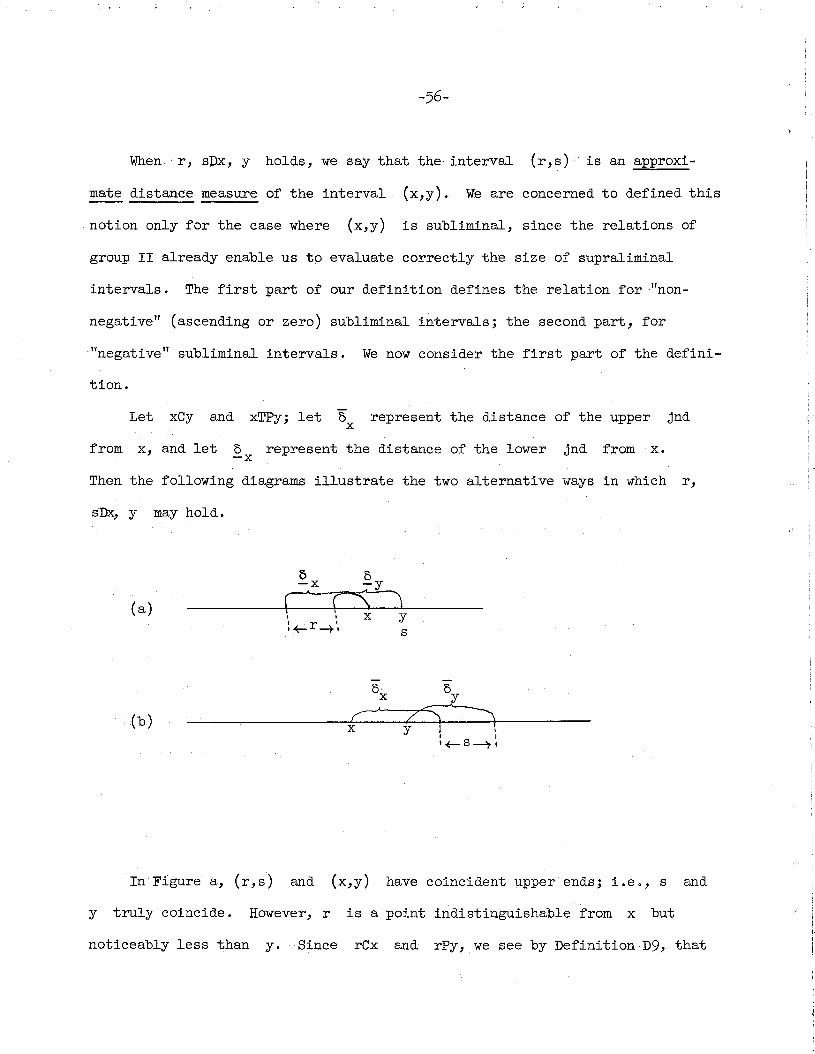
-56-
When r, sDx, y holds, we say that the interval (r,s) is an approxi-
mate distance measure of the interval (x,y). We are concerned to defined this
notion only for the case where (x,y) is subliminal, since the relations of
group II already enable us to evaluate correctly the size of supraliminal
intervals. The first part of our definition defines the relation for IInon-
negative" (ascending or zero) subliminal intervals; the second part, for
"negative" subliminal intervals. We now consider the first part of the defini-
tion.
Let xCy and xTPy; let "5x represent the distance of the upper jnd
from x, and let 5 represent the distance of the lower-x jnd from x.
Then the following diagrams illustrate the two alternative ways in which r,
sDx, Y
(a)
(b)
may hold.
" " x y.+-r---4-, s
In Figure a, (r,s) and (x,y) have coincident 1.lpper ends; Le., s and
y truly coincide. However, r is a point indistinguishable from x but
noticeably less than y. Since rCx and rPy, we see by Definition D9, that

-57-

(c)
(d)
-58-
I Y XI
• I rl~s -?:
In Figure c, (r,s) and (x,y) have trUly coincident upper ends, while
the lower end of (r,s) though indistinguishable from the lower end of (x,y)
is noticeably less than the upper end of (x,y). That is, x and r coincide,
while s lies to the left·of y somewhere between the left-hand end of the
lower jndfrom x and the left-hand end of the lower jnd from y.
In Figure d, (r,s) and (x,y) have truly coincident lower ends but
the upper end of (r,s), though indistinguishable from the upper end of
(x,y) is noticeably greater than the lower end of (x,y). That is, y and
s coincide, but r lies to the right of x somewhere between the upper end
of the upper jnd from y and the upper end of the upper jnd from x.
Comparing our diagrams a and bwith c and d, respectively, we note at
once that the conditions under which (rs,) is a distance measure of a
negative interval (x,y) are exactly those required for (s,r)to be a
distance measure of the positive interval (y,x). Similarly, if r, sDx,y,
where (x,y) isa positive interval, We have automatically that (s,r)

-59-
is a distance measure of the negative interval (y,x). The reversal of
the variables involved in the convenient equivalence: r, sDx, y if and
only if s, rDy, x, (Theorem 45), corresponds to the appropriate change
.of "sign" in the intervals under consideration. Our definition is such
that the distance measure of a negative interval will itself always be a
negative interval, while the distance measure of a positive interval will
be positive (Theorems 43, 44). Hence, a distance measure interval (r,s)
reflects not only the absolute distance of a subliminal interval (x,y)
but also its direction.
An examination of diagrams c and d reveals that the size of a nega-
tive subliminal interval (x,y) may roughly be considered to be the
size of its minimum (greatest in negative extent) "distance measure
interval" plus the jnd. More precisely, (since there may be no such
minimum distance measure interval), the size of a negative subliminal·,
interval (x,y) is obtained ~y adding 6 to the greatest lower bound
of the magnitudes of its distance measure intervals.
Definition D13 is so central to our system that it is worth noting
some comparisons with notions suggested by Wiener and Goodman in their
attempts to provide for the accurate orderings of subliminal intervals.
Wiener regards a subliminal interval as the difference between two
supraliminal intervals with coincident upper·or lower ends. It may be
that our notion D in effect pins down this suggestion of Wiener IS.
Thus. (x,y) in our figure a may be approximately defined as the dif-
ference between the maximum distance measure interval (r,s) and the
interval (r,x), illustrating the first possibility if we stretch a

-60-
point to regard (r,x) as supraliminal; actually, of course, such an interval
(r,x) is the maximum possible descending subliminal distance from x. Again,
in figure b, (x,y) may be regarded as the difference between two supraliminal
intervals (r,s) and (y,s) with coincident upper ends. Wiener's discussion,
however, is difficult and obscure. His remarks do not in any straightforward
manner relate this method of defining a subliminal interval to a method for
estimating relative sizes of subliminal intervals, and much of his discussion
suffers from obscurity due to the figurative character of his language. (ThUS,
he writes: ."the vector corresponding to a subliminal interval may be defined
in terms of two supraliminal vectors whose difference it forms, as the rela
tion between two terms when one either first ascends an interval belonging
to one, and from that point descends an interval belonging to the other, or
first descends an interval belonging to the second, and then ascends an
interval belonging to the first." (Wiener [29], p. 185.)
The similarity of our relation D to a notion employed by Goodman is
more easily seen. Goodman defines for pairs of qualia (x,y) a function
x ty which is the sum of all qualia which match x or y but not both,
(Goodman [9], p. 239), and suggests that the size ofxty is a first
approximate measure of the qualitative distance between x and y. Since
our ontology is not finite, we do not speak of "sums" of elements in our
system, but if we were to substitute the notion of an interval for Goodman's
notion of a sum, then we might, by analogy with Goodman, consider the interval
of all points which are indistinguishable from x ory but not both to be
the rough distance measure of the size of a subliminal interval (x,y). This
approach, though intUitively plausible,encounters a certain difficulty.

-61-
Consider a positive subliminal interval (x,y) of a specified size ex
in the middle of a sensory range. Then the interval of all points match
ing x or y but not both will extend to the left of x by the distance
of the lower jnd from x and to the right of y by the distance of
the upper jnd from y. Supposing the uniformity of jnds, then the
distance measure interval for (x,y) will equal a + 2,6. Now suppose
that at the top of a sensory range there is another positive subliminal
interval (z,w) exactly equal ,in sensory distance to (x,y). The
interval of all points matching z or w but not both will extend to
the left of z by a distance of 6, but since w is our maximum sensa
tion, w must be the upper terminus of the interval. That is, the
distance measure for (z,w) will be given by adding 6 only once to
the size of (z,w), and will equal, a + 6. Since (x,y) and (z,w)
are the same size, their distance measure intervals should also be the
same. The fact that this condition can be violated under the proposed
approach leads us to a definition which will not encounter the outlined
difficulty when a limited sensory range is considered. For this reason,
we define the distance measure of an interval (x,y) as the interval
from a single end-point of (x,y) to a point from which the given end
point is distinguishable, but from which the other end-point is not.
The span is defined in terms of a distance from only one end-point of the
subliminal interval, lower or upper according tban option provided by
the alternative formulation of the definition, and essential to the
requirements of a limited sensory range. Thus for a positive subliminal
interval, (x,y), in the neighborhood of the maximum possible sensory
magnitude, clearly the distance interval must be chosen in a downward

-62-
direction from the right-hand end of the interval as in figureaj in the
minimum range of magnitudes, only an ascending distance measure extending
from the left-hand end of the interval as in figure b would serve.
It is apparent that our notion, D} diverges in certain respects from
analogous concepts introduced by Wiener and Goodman, However, in common
with the latter notions, our relation D is chiefly important as providing
a reduction of the problem of ordering subliminal intervals. We note from
our definition that a distance measure interval, (r,s), is always supra
liminal. (Theorems 43, 44.) But we already have a criterion for the
relative magnitudes of supraliminal intervals (Definition D7). The device
used irt our next definitions is to develop an indirect test for the rela
tive sizes of subliminal intervals in terms of comparisons of the distance
measure intervals respectively characterizing these intervals. The
significance of Definition D14 lies entirely in this respect.
The numerical interpretation forD is that
(i) if xCy and xTQy, then r, sDx, y if and only if cp( s) - cp( r)
< cp(y) - cp(x) + 6·
(ii) if xCy and yTPx, then r, sDx, y if and only if cp( r) - cp( s )
< cp(x) - cp(y) + 6.
Finally, we note a fact of even greater numerical significance for our
further definitions, which is proved in our representation theorem but which
should be fairly intuitively obvious from our definition of D and its
numerical interpretation. If, for any positive subliminal interval (x,y),
we define the set [5(x,y)
to be the set of all numbers a representing

-63-
the sizes of distance measure intervals of (x,y), then
(1) the least upper bound of 1) ( ). = cp(y) - cp(x) + 6,.x,y
Definition D14. GL is the quaternary relation defined as follows:
( i ) if (xCy and zCw) and (xTQy and zTQw), then x, yGLz, w
~ C3u)(3 v)[u, vDz, w & (r)(s)(r, sDx, y ~ r, sTLu, v)].
(ii) if (xCy and zCw) and (either yTPx or wTPz), then
x, yGLz, w~ (] r)(3 s)[r, sDx, y& (u)(v)(u, vDz, w ~r, sTLu, v)].
(iii) if not xCy .or not zCw, then x, yGLz, w~ x, yTLz, w.
GL is the relation of genuinely less than between intervals. The
definition is presented in conditional form, but could obviously be made
explicit if the hypothetical formulations of each condition were con
joined as a total disjunction of conditionals. The first and second
parts of the definition, (i) and (ii), define the relation GL for the
case where both intervals compared are subliminal; in (i), both sublimihal
intervals are non-negative; in (ii), at least one of the intervals is
negative. The third part of the definition relates pairs of intervals,
at least one of which is supraliminal. Thus the definition is clearly
exhaustive of the possibilities, and provides for the comparison of any
two intervals whatsoever. By (iii), we see that our criterion of relative
magnitude for pairs of intervals not both subliminal in size reduces to
the TL relation defined in Definition D7. The interest of Definition
D14, therefore, centers in parts (i) and (ii) . We consider only part
(i), since our remarks may easily be extended to part (ii), and since,
by the theorem that x, yGLz, w if and only if w, zGLy, x, (Theorem 51),

-64-
we can reduce many 'of our comparisons of negative intervals to comparisons
of positive intervals.
Definition D14 (i) states that a non-negative subliminal interval (x,y)
is genuinely less than another such interval (z,w) if and only if there is
some distance measure of (z,w) which is truly greater than all distance
measures of (x,y). We now justify this definition, using primarily the
numerical facts stated in (1).
We first show the proposed condition to be necessary. Suppose a non-
negative subliminal interval (x,y) to be of genuinely smaller size than
another interval (z,w); numerically, ~(y) - ~(x) < ~(w) - ~(z). Clearly
(z,w) must be positive, while (x,y) may be zero or positive. Our axioms
guarantee that any positive subliminal interval possesses a distance measure.
(Theorem 42.) But if xTCy (i.e., if (x,y) is a zero interval), then no
distance measure can be found for it, since there will be no point distin-
guishable from x or y but not both. (Theorem 41.) Hence, there is a
distance measure of (z,w) which, vacuously, is greater than all distance
measures of (x,y); and the definition is satisfied for this case. Now
suppose that xTPy (i.e., (x,y) is positive), and suppose that D14 (i) is
not satisfied. Then no distance measure of (z,w) is greater than every
distance measure of (x,y). Hence the least upper bound of tJ(z,w) is not
greater than the least upper bound of n( But by (1), this yields:x,y) .
~(w) - ~(z) + 6 < ~(y) - ~(x) + 6; and we derive ~(w) - ~(z) :::: ~(y) - ~(x),
contradicting our assumption that (x,y) is genuinely less than (z,w).
We next show that if the criterion stated by Definition D14 (i) is met
by appropriate intervals (x,y) and (z,w), we must have (x,y) genuinely

-65-
less than (z,w). That is, we show that the condition is sufficient.
Assume that (u,v) is a distance measure of (z,w) greater than all
distance measures of (x,y). Then we know by (1) that
(2) ~(y) - ~(x) + ~ ~ ~(v) - ~(u).
But by Definition D13 (i), we see that since u,vDz, w, then one of the
situations illustrated in the following two diagrams must hold:
(i)
(ii)
o 0z w
~
u
: \ z wIf-- u -7-', v
Intuitive considerations (capable of formal proof) make it obvious that
in case (i),
~(v) - ~(u) = (~(v) - ~(w)) + (~(w) - ~(z))
while in case (ii),
~(v) - ~(u) = (~(z) - ~(u)) + (~(w) - ~(z)).
-66-
But then since for case (i), by Definition D13 (i), we must have wCv, and
for case (ii), we must have uCz, our numerical interpretation for C gives
us for either case that
~(v) - ~(u) < ~(w) - ~(z) + A.
Referring to (2), we derive the desired result:
~(y) - ~(x) < ~(w) - ~(z).
We note that our entire justification for this definition depends on the
condition stated in (1) which in turn presupposes the uniformity of the jnd
in the sense discussed under Definition D12. In effect, the definition
asserts that a non-negative subliminal interval (x,y) is less than another
such interval (z,w) just in case the least upper bound of the magnitudes
of the distance measures of (x,y) is less than the least upper bound of
the magnitudes of the distance measures of (z,w). Granted that for every
interval (x,y), the least upper bound of !)(x,y) equals the size of
(x,y) plus a uniform A representing lithe Ii size of Iitheli jnd, the asser-
tion is clearly correct. But omit the latter assumption for a moment, and
consider how without it, the stated criterion might give intUitively incorrect
results. Suppose, first, that ascending (or descending) jnds fromdifferent
points differed in magnitude; and suppose that (x,y) and (z,w) were both
positive intervals at the minimum range of sensation so that for both intervals
distance measures could be found only in an upward direction. Then by Defini-
tion D13, the least upper bound for (x,y) must be equal in size to the
distance of (x,y) plus the distance of the upper jnd from y; the least
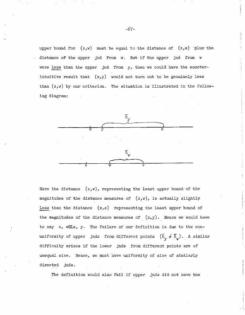
-67-
upper bound for (z,w) must be equal to the distance of (z,~) plus the
distance of the upper· jnd fromw. But if the upper jnd from w
were less than the upper jnd from y, then we could have the counter..
intuitive result that (x,y) would not turn out to be genuinely less
than (z,w) by our criterion. The situation is illustrated in the follow-
ing diagram:
z
cy
c:w
oY
--A-------~
s
"5w
v
Here the distance (z,v), representing the least upper bound of the
magnitudes of the distance measures of (z,w), is actually ~lightly
less than the distance (x,s) representing the least upper bound of
the magnitudes of the distance measures of (x,y). Hence we would have
to say z, wGLx, y. The failure of our definition is due to the non-
uniformity of upper jnds from different points (By ~ Bw)' A similar
difficulty arises if the lower jnds from different points are of
unequal size. Hence, we must have uniformity of size of similarly
directed jnds.
The definition would also fail if upper jnds did not have the

-68-
same size as lower jnds. Suppose, for eXaJIlple, we wished to compare an
interval (x,y) at the minimum end of the scale with an interval (z,w) at
jndsexample, lower
'5 ; while they
plus 0 If, for-z
Then the least upper bound of JJ would(x,y)
least upper bound of J)(z,w)
the maximum end of the scale.
equal the size of (x,y) plus
would equal the size of (z,w)
were always less than upper jnds, we might arrive at a counterintuitive
result illustrated below:
oy
x y)s
u z w
Here (u,w) representing the size of the least upper bound of distance
measures of (z,w) is less than (x,s), representing the size of the least
upper bound of distance measures of (x,y), and our criterion compels us to
say z, wGLx, y, contrary to the actual sizes of the intervals. Our defini-
tion, therefore, requires the uniform size of all jnds whatsoever. We
have already seen that our axioms guarantee this condition; but it is worth
noting the strong requirements for the justification of this definition.
The numerical interpretation of GL is that of strict algebraic
inequality between intervals (without any conditions on the intervals): x,

-69-
yGLz, wif and only if ~(y) - ~(x) ~ ~(w) - ~(z).
Definition D15. x, yGEz, w~ rv x, yGLz, W &NZ, wGLx, y.
GE is the relation of genuine equality between intervals. Two
intervals are genuinely equal when neither is genuinely less than nor
genuinely greater than the other. For positive subliminal intervals,
this is to say that for every distance measure of one of the two
intervals, there is a distance measure of the other interval at least
as great. (For negative subliminal intervals, we change the last
statement to read: "at least as smalL Ii) When one of the related
intervals is supraliminal, genuine equality holds where true equality
holds. The criterion for equality presented in Definition D15 is
intuitively correct for all types of intervals.
As numerical interpretation for Definition D15, we have strict
algebraic equality between intervals: x, yGEz, w if and only if
~(y) - ~(x) = ~(w) - ~(z).
Definition D16. x, yGRz, W~rV z, wGLx, y.
Two intervals stand in the relation GR to one another just in
case the first is not genuinely greater than the second.
The numerical interpretation for this notion is one of loose
algebraic inequality between intervals: x, yGRz, w if and only if
~(y) - ~(x) ~ ~(w) - ~(z).
IV. "Ratio li Relations. We are now in a position to define a group
of notions which allow for the expression of quantitative relations

-70-
between intervals. We first define two notions (Definitions D17 and D18)
which enable us to consider the length of an interval as a multiple of a
subinterval; the notions permit us to consider fractional parts of intervals;
and our final definition (Definition 19) allows for the comparison of such
fractional parts of intervals. From such a relation, it is clear that we
may infer the numerical ratio of two intervals to one another. This notion,
therefore, is of prime importance in the achievement of measurement proper,
as will be apparent in the proof of our representation theorem.
The definitions introduced in this section are exactly analogous to
notions employed in the Suppes-Winetaxiomatization of utility, except for
the fact that here we have not defined a notion of "betweenness. 1i We there-
fore make only brief comments on each notion, and refer the reader to Suppes
and Winet [27], pp. 261-265 for further discussion.
For brevity in introducing these notions, we first lay down the follow-
ing convention:
Convention. Variables 'm', In', 'p' take as values non-negative
integers; variables 'a', 'bY, 'c', 'd' take as values positive integers.
Definition D17. x, yGMu, v M yTCu & [(xTPy & yTPv )v( vTPy & yTPx)]
& x, yGEu, v.
To say, x, yGMu, v is to say that (x,y) and (u,v) are adjacent
equal intervals.
This relation is useful chiefly when we deal with powers of GM. The
thn power of GM is defined recursively:
x, YG~z, w H x, yGMz, w;

-71-
x, yGlCz, w~ C3 u)( j v)(x, YGM(n-l)u, v & u, vGMz, w).
Thus, to say that 2x, yGM z, w is to say that (x,y) is adjacent
and equal to an interval (u,v) which in turn is adjacent and equal to
the interval (z,w). In other words, (x,y) and (z,w) are equal, and
there is a further interval of the same length lying between them.
Clearly, (x,w) will be three times the length of (x,y). In general,
to say that cx, yGM z, w is to say that the length of (x,w) is (c+l)
times the length of (x,y).
Definition D18. GN(a) is the quaternary relation defined as
follows:
(i) if a = 1, then x, yGN(a)u, v~ xTCu & yTCv;
(ii) if a ~ 1, then x, yGN(a)u, v<E;-7 xTCu & C3 z)(x, YGM(a-l)z,v).
This notion explicitly formalizes the length relation of an interval
to its sub-part which has been suggested by the GM relation. We inter-
pret x, yGN(a)u, v intuitively as meaning that if an interval of the
length (x,y) is iilaid off ii a times in the appropriate direction, we
obtain the interval (u,v). Thus we can express the fact that (u,v)
is a times the length of its subinterval (x,y); or, alternatively that
(x,y) is (lja) th part of (u,v) .
The numerical interpretation of DefinitionD18 is that x, yGN(a)u, v
~ ~(v) - ~(u) = a(~(y) - ~(x)).
Definition D19. GH(m, a; n, b) is the quaternary relation such
that x, yGH(m, a; n, b)u, v ~ (3 zl)(3 z2)(::! wl)(3w2)(x, Zl GN(2m
)x, y
& x, zlGN(a)x, Z2 &u, wl GN(2n
)u, v &u, wlGN(b)u, W2 &x, z2GRu, w2).

-72-
When we say that x, yGH(m, a; n,b)u,v, we express the fact that an
(a/2m)th h 1part of t e interva (x,y) . t t th (b/2n )th part1S no grea er an a
of the interval (u,v). This method of comparing the size of two intervals
in terms of respective submultiples of each is chosen over a method which
would define the ratio of one interval to another in terms of respective
multiples of each. For example, we might have chosen a relation which would
enable us to express the fact that four times an interval (x,y) was not
greater than three times an interval (z, w) • Both methods would equally
allow us to estimate the ratio of one interval to another, but the compari-
son of intervals in terms of their submultiples rather than their multiples
has the advantage noted by Wiener IIthat we do not wish, for example, the
existence of a loudness 9,999,999,99910,000,000,000
as great as that of the falling
of a pin to depend on that of a loudness 9,999,999,999 times as great as
that of the falling of a pin." (Wiener [29], p. 186.) The essentially
limited range of sensation demands a definition of the sort we have given
for determining the ratio of two sensory intervals.

will be said to be a JUST NOTICEABLE DIFFER---------
-73-
IV. AXIOMS
For purposes of brevity and intuitive clarity, the statement of our
axioms is given in terms of the notions defined in the previous section,
as well as our primitives K and L.
~ system ~= <K, L >
ENCE STRUCTURE if the following fifteen axioms are satisfied for every
x, y z, w, u and v in K:
Axiom Al. It is not the case that x, yLx, y.
Axiom A20 If x, yLz, wand z, wTLu, v, then x, yLu, v.
AxiomA3. If x, yLz, w, then w, zLy, x.
Axiom A4. If xCy, then x, yLz, w if and only if zPwo
Axiom A5. If xPy, then x, yLx, z if and only if ypzo
Axiom A6. If xPy, then x, yLz, y if and only if zPxo
Axiom A7. If xTPy and yTPz, then x, yGLx, z and y, zGLx, z.
Axiom A8. If x, yGEu, v and y, zGEv, w, then x, zGEu, w.
Axiom A9. If x, yGEv, w and y, zGEu, v, then x, zGEu, w.
Axiom AlO. There is a z* in K such that, for every x, z*Qx.-- --Axiom All. Either there are elements y and z in K such that-----
xJPy and yJPz, or there are elements v and w in K such that xJFv----and vJ:Fw.
Axiom A12. There is a t in K such that x, tGEt, y.
-74-
Axiom Al3. If xTPy and x, yGLu, v, then there is a t in K such--that uTPt and tTPv and x, yGEu, t.
Axiom A14. If xTPy and x, yGLu, v, then there is an s in K such'--,- -,-
that uTPs and sTPv and x, yGEs, v.
Axiom Al5. If xTPy and x, yGRu, v, then there are elements s and t
in K and ~ positive integer such that c and sGRx,c u, sGM t, v u, y.----Axiom Al expresses the fact that L is irreflexive; or by Definition Dl,
that an interval seems equal to itself. The axiom is open to obvious question
on empirical grounds, since, in the area of sensation, a sense-difference
between identical stimuli may vary in size from one time to another; while,
on the other hand, it is impossible to compare a sensory interval with itself
at anyone moment, a lapse of time being required for the comparison. The
necessity for such an axiom is a good illustration of the inevitable idealiza-
tion of the empirical situation required for developing a formal scheme of
measurement.
Axiom A2 expresses the fact that if an interval seems less than a second
interval which is truly less than a third, then the first seems less than the
third. The axiom may be justified by considering that the second interval, if
it does not actually~ less than the third, must at least seem equal to it.
In either case, it is natural to suppose that the
than the third.
Axiom A3 expresses a "sign reversal" property. An interval seems less
than another interval if and only if the second seems less than the first
when the intervals are considered in reverse direction, i.e., when the
"negatives"·ofthe intervals are considered. This axiom represents the fact

-75-
that we are construing intervals as "signed" or "directional-it Ifwe
were dealing only with absolute distances, the "sign" of the interval,
or the order of its component end-points, would be indifferent to its
size. The axiom corresponds to the arithmetical fact that if a < ~,
then -~ < -a.
Axiom A4 is perhaps the axiom most central to our system. It
expresses the fact that any subliminal interval seems less than any
supraliminal interval. The assumption is apparently innocuous and
undeniable. It is, in fact, the only axiom which Wiener's study expli
citly mentions. He writes: IIwe shall suppose it to be axiomatic that
in any intrinsic comparison of differences between intervals 7 a subliminal
or unnoticeable difference is always to be treated as less than a notice
able difference." (Wiener [29], p. 185.) The use of this axiom also
receives support from Goodman's work although he refers to the condition
as an "extra-systematic rule of order" rather than an axiom, a point we
have already questioned. Goodman states this rule as follows: "the
span between any two matchingqualia is less than the span between any
two non-matching qualia." (Goodman [9], p. 241.) But the persuasive
character of these verbal formulations conceals the real power of this
axiom.
In the first place, the axiom in effect re-introduces the infinite
discrimination we have tried to eliminate by not assuming a transitive
indifference. (This was first pointed out to me by Professor Davidson.)
The assumption is that no matter how small the difference in actual size
between a subliminal and a supraliminal interval, the former is

-76-
distinguishable from the latter. To put it another way, suppose (x,y) to
be a positive subliminal interval of almost maximum subliminal size. Suppose
y to be indistinguishably less than z, (y seems equal to z, though it is
not identical with z). We would under such circumstances, since y and z
are indistinguishable, expect (x,y) to seem equal to (x,z). But if (x,z)
happens to be a supraliminal interval, this will not be so. The axiom seems
to contain an internal discrepancy. On the one hand, it asserts that any
two intervals between matching elements will seem the same, no matter how
disparate in actual size. On the other hand, an interval between almost
discriminable elements will be distinguishable from an interval between just
discriminable elements, though the actual sizes of the two intervals may be
almost identical.
x z y w
Thus, in the diagram, (x,z) will be indistinguishable from (x,y), but (x,y)
will be clearly less than (x,w); though in the first comparison, the actual
size difference is greater than in the second.
A second feature of the axiom which might easily be over looked is its
implication (al least in connection with other plausible assumptions) of the
uniformity of the jnd. Goodman rejects taking the spans between just-
noticeably different qualia as uniform, (Goodman [9], po 241) in favor of the
IImore relative uniformity" suggested by his "rule li and our liaxiom. II But it

-77-
seems to us that the axiom requires a constant jnd. For assume one jnd,
(x,y), to be less than another jnd, (z,w). Then it is reasonable to
suppose that we can "lay off ll within the larger· jnd (z,w) an interval
(z,t) equal to the smaller of the two jnds. (Axiom Al3.) Since
(z,t) lies entirely within a discriminable threshold, it must itself
be subliminal; and since it is equal in actual size to (x,y), the two
intervals will presumably seem equal. (A realistic system for sub
liminal differences does not assume that seeming equality implies actual
equality. However, actual equality is presumed to appear as equality.
(Theorem 3.)) But (x,y) can seem equal to (z,t) by Axiom A4 if and
only if it is itself subliminal, and hence it cannot constitute a jnd
contrary to our assumption. Thus any two jnds must be genuinely equal.
Finally, we note a certain verbal confusion in connection with
Goodman's and Wiener's remarks on the condition we are discussing which
suggests the necessity of an even stronger uniformity of jnds. Wiener
says If a subliminal ... difference is to be treated as less than a notice
able difference. If Goodman says that the span between matching qualia is
less than the span between non-matching qualia. The point to note is the
'use of the word 1I1ess ." While it is undeniable that a non-noticeable
difference~ less than a noticeable difference, it is not so clear
that we could substitute "is ll for "seems" and get a true statement (as
Goodman and Wiener seem to have done) without assuming a uniform jnd.
For if we interpret the jnd as non-uniform it is not impossible to
. consider intervals possessing the characteristics illustrated in the
following diagrams~

-78-
Ox Oy
c-:: c:s--A
:)X Y z
u v w
(x,y) is a positive subliminal interval lying within the upper jnd from
xi (y,z) is a positive subliminal interval lying within the upper jnd from
y, and all three points x, y and z occur at an area of the scale where
the jnds are fairly large.
On the other hand, (u,v) and (v,w) are adjacent positive jnds
occurring at an area of the scale where the jnds are relatively small.
Clearly, by Axiom A4, (x,y) will seem less than (u,v) since the former
in contrast to the latter is a non-noticeable difference. Similarly (y,z)
will seem less than (v,w). But can we infer that (x,y) and (y,z) are
less than (u,v) and (v,w)? If so, then surely, in accordance with the
arithmetical laws governing inequalities we must admit that (x,z) is less
than (u,w). But suppose, as in the diagram, that (u,w) seems less than
(x,z) (Le., (u,w) differs from (x,z) by more than a jnd). Then we are
involved in a contradiction, for in the case of (x,z) and (u,w), "seeming"
less does not involve "being" less. But we have assumed for the smaller
intervals in question that it did. The difficulty, of course, could not
arise if we assumed a constant size of jnd, and it seems to us that any
system which assumes that "seeming less" implies "beingless" must postulate

-79-
the strong form of uniformity of jnds discussed in our introduction:
namely, the equality of all n-chains of jnds.
The conjecture just discussed, namely the impossiblity under
various conditions ofaxiomatizing the notion of a non-uniform jnd,
receives some support from the axiomatization of semi-orde~s given by Scott
and Suppes ([20]). Their proof that any semi-order may be given a numeri
cal representation with a constant jnd throughout the whole scale shows
that Luce's sup and inf constructions are weaker than they need to be, or,
in other words, that Luce really has a uniform jnd. It would be inter
esting more fully to investigate this conjecture against the assumptions
of Goodman and Luce.
AxiomsA5 and A6 assert in part that positive supraliminal intervals
with an identical end-point are distinguishable only if their nOn-identical
end-points differ noticeably. We contrast this assumption with Axiom A4
which allows for intervals with an identical end-point to be distinguish
able even when their non-identical end-points do not differ noticeably- in
the special case where one of the compared intervals is subliminal, and
the other supraliminal. We have already mentioned the dubious nature of
the special assumption made in Axiom A4. Axioms A5 and A6, on the other
hand, seem entirely reasonable in this regard. The remaining content of
A5 and A6 refers to the "sense" of L. Axioms Al-A3, for example, do not
reveal whether L is to be interpreted as noticeably less than or notice
ably greater than. The latter interpretation is disallowed by Axioms A5
and A6 which together state, in effect, that if a point y lies noticeably
between two points x and z, then x, yLx, z and y, zLx, z. This

-80-
requires that L be interpreted as noticeably less than.
Axiom A7, using the notion of a point lying "truly between" two other
points similarly establishes the "sense" of GL as genuinely less than.
Axioms A8 and A9 express the fact that the "addition" of genuinely equal
adjacent intervals yields genuinely equal intervals. These axioms, we note,
.provide for the genuine equality of jnd chains, once the genuine equality
of any two jnds to .one another is assured.
Axiom AlO is our Ii absolute threshold" axiom. It asserts that there is
some element, z*, such that no other element is discriminably less than z*.
In other words, any discriminable element must seem at least as great as z*.
All other discernible stimuli, if not greater than z*, must lie within the
lower jnd from z*. z* thus corresponds approximately to the lowest
di~criminable or lithreshold" stimulus. It has sometimes been suggested that
such an element is a "zero" element. Thus Stevens and Volkmann refer to the
lowest tone of an organ as a Yizeroll pitch. (Stevens and Volkmann [23].) We
cannot agree. A stimulus of Yi zero" pitch would be one of "zero,Yi or no sub
jective magnitude, and hence indiscriminable. Hence no discriminable stimulus,
even the least, can be said to correspond to zero. The search for a natural
"zero" in subjective domains has taken other forms. McNaughton, for example,
has suggested that the state of unconsciousness constitutes a natural zero
for a metric of happiness. (McNaughton [15].) Unconsciousness, presumably,
has no subjective magnitude, positive or negative, and McNaughton, therefore,
avoids the type of mistake made by Stevens in referring to the lowest tone
of the organ as zero. Similarly, Reese seems to suggest that Stevens might
correctly have taken as zero the first tone arousing no sensation of pitch.

-81-
(Reese [18], p. 30.) If we accepted such views then we would in effect
be able to speak of a zero element if the element z* specified by
Axiom A4 were taken as the element just noticeably greater than the zero
element. But it seems to us that such procedures are invalid. A state
or stimulus arousing no sensation at all cannot be scaled by observer
responses, and therefore, has no place (not lYzeroli place) on a sensory
scale. Or, to put it differently, since we can say with equal truth
that unconsciousness, a blue light, and a sound wave of frequency less
than that of the lowest tone on the organ arouse in the observer no
pitch sensation at all, there seems as good reason for equatinguncon
sciousness or blue with the natural zero of a pitch scale as there is
for equating it to a sound wave of a certain frequency. Clearly, this
is absurd.
The use of Axiom AIO, therefore, cannot be taken to mean that we
assume the existence of a natural zero for subjective magnitudes. It
is slightly more plausible to suppose that Axiom AlO implies the exist
ence of a natural unity element, since it does assert that z* is a
lYfirst lY sensible element. It seens natural to think of assigning the
number 1 to z*, 2 to the next noticeably higher element, etc.
Unfortunately, however, we must forego the attendant advantages of
having a natural unit unique up to an identity transformation. There
is nothing in our axiom which requires that z* be assigned the number
one rather than two, four, or n so long as no other element is
assigned a number less by more than the size of the jnd than that
given to z*; moreover, any number assigned to represent the length of

-82-
the jnd may be multiplied by a positive constant without distorting a
correct assignment of scale values. To have equal scale units in, say, the
sense of uniform jnds does not insure the same uniqueness of scale that
exists in counting. In the sense that we can transform our unit by any
similarity transformation that we please, we cannot consider it a "natural"
unit.
We remark that we have not assumed a "maximum" element. The proof of
our representation theorem requires only a system bounded at one end.
Axiom All is our "differential threshold" axiom. It states that any
element is either just noticeably less than a second which in turn is just
noticeably less than a third, or that the given element is just noticeably
greater than a second which is itself just noticeably greater than a third.
In other words, given any element, there are two further appropriately
spaced elements such that we can proceed upwards or downwards by a distance
of two jnds. It can be shown that Axiom All requires that any model of
our system have a "length" of at least three jnds. For by the axiom,
clearly, we must have at least three just noticeably distinct elements,
x, y and z. Let us suppose they lie in the order indicated in the follow-
ing diagram:
x y z
We easily see that to ensure that All is satisfied for y, the midpoint of
the three points, there must be a fourth element lying either to the right

of zby a distance of one jndor to the left of x by the same
distance; the two alternatives are shown in the following diagrams:
x y z
v x y z
Hence no model for our system can consist of less than four points, nor
can it possess a total "distance" of less than three jnds. This con-
dition is of mathematical interest, although empirically trivial.
Clearly, both conditions listed as alternates in the axiom are
required, since a maximum element could not be noticeably less than
any other element, and a minimum element (such as z*) could not be
noticeably greater than any other element. Other elements, however,
will in general have jnds in both directions. The differential
thresholds, of course, provide us with the "stepsll by which we pass
from one element to another. Since we have shown that, for our system,
these "steps" must be equal, they provide us with our unit of measure-
ment.
AxiomAl2 is interpreted to mean that between any two elements of
K, there is a midpoint; that is, a point which bisects the "genuine"
distance between the two given points. "Bisection ll and "fractionationll

-84-
procedures, as used by Stevens, require the subject to select stimuli which
seem to be midpoints between two other stimuli; however, the experiments do
not provide sufficient checks to insure that these points do genuinely
bisect the intervals. The widespread use of such "bisection" procedures
in psychology, therefore, cannot be taken as justification for the axiom
as stated here. Utility experiments recently conducted at Stanford do
aim at the genuine bisection of subjective intervals, and attempt to
achieve this goal in terms of inference from apparent bisections. A
similar course is suggested by our definition of "genuine equality" in
terms of a chain of notions originating in a notion of "seeming equality."
However, the Stanford group was only able to approximate such genuine
midpoints, in terms of specifying upper and lower bounds or "nests" with
in which they must lie. (Davidson, Siegel and Suppes [7].) It is not
clear, therefore, that at the present time this axiom has been proved
capable of verification.
Axiom A12 is obviously of central importance to our scheme of measure
ment since it establishes the existence of equal adjacent scale units. Any
scale of such units would furnish a type of measurement; among such possible
units, we choose adjacent jnds to yield jnd measurement.
Axioms A13 and A14 specify that if a truly positive interval (x,y)
is genuinely less than another interval (u,v), then two intervals genuinely
equal to (x,y) can be "laid off" along (u,v) in such a way that one of
the end-points of the I1laid off l1 interval coincides with the corresponding
end-point of (u,v). One of these intervals will have its initial end-point
coincident with u, while its terminal end-point lies to the left of v. The

-85-
other interval will have its terminal end-point concident with v while
its lower end-point lies to the right of u.
Axiom Al5 is our Archimedian axiom. It asserts that if the differ
ence between x and y, where x is truly less than y, is not greater
than the difference between u and v, then there are c equally spaced
elements of K between u and v such that the difference between any
two of them is not greater than the difference between x and y. In
other words, any interval at least as great as a second interval may be
exactly subdivided into adjacent and equal fractional parts no greater
than the second interval.
Axioms Al3, Al4 and Al5 enable us to compare non-adjacent intervals
in terms of equal units, by contrast with Axiom Al2 which accomplishes
this result only for adjacent intervals.
A few general remarks may be made about our axioms. We note that
they fall into three groups. The first group, Axioms Al-A6, specifies
properties of our "seeming" relations only (With the exception of A2
which involves a litrue"relation as well). The second group of axioms,
A7-A9, concerns our more complex set of defined notions, our "genuine"
relations. Finally, the third group of axioms, AlO-Al5, are "existence"
axioms, specifying the liexistence li of certain elements of K in terms
of "seemingli , litrue" ligenuineli and lI ratioli relations. Obviously, we
would have a simpler, more perspicacious set of axioms if all of the
linon-existence" axioms like Axioms Al, A3-A6 stated properties of only
"observable" relations, and if the "existenceli axioms specified elements
in terms of "seemingli relations alone (as in Axiom AlO) . Such a set of
-86-
axioms would certainly be more in keeping with intuitive demands; for the!
problem at hand seems to be one of answering the question: what notice-
able elements must exist, and what properties of relative apparent size of
elements and intervals must hold in order to allow for the inference of a
jnd structure? We seem here to be postulating the jnd structure, the
indiscriminable elements and differences and their relative positions,
rather than inferring them. To a certain extent, this criticism is
unjustified since axioms on our more complicated notions may be trivially
rewritten in terms of our simpler notions alone by substituting defiriiens
for definiendum wherever the definiendum is not a II seemingli relation. But
the objection is nevertheless pertinent, since an attempt to rewrite such
an axiom as Axiom A7, for example, reveals the complexity of the assumptions
we are making about the character of what T1 noticeablyll holds. It would be
desirable to eliminate II strongli axioms of this sort in favor of IIweaker li
axioms on the lIapparentli relations of our system. In some cases, such as
Axiom A7, it seems reasonable to suppose this is possible. In the case of
our· llexistence ll axioms, however, it seems less plausible to assume the
eliminability of the axioms on II genuine II relations in favor of· IIweaker,1I
(non-equivalent), axioms on II apparent II relations. Axiom A12, for example,
seems essential to our IImidpoint li method of achieving interval measurement
for subliminal as well as supraliminal intervals. Despite such qualifica-
tions, we feel quite sure that a more elegant and intuitively satisfying
set of axioms may sometime be achieved for jnd measurement. Ourrepre-
sentation theorem (Section 6), however, will show that the set of axioms
here presented is at least adequate for such measuremerit; and it is to be

-87-
hoped that our result may serve as a foundation for an eventual scheme
of greater simplicity and clarity.

-88-
V. ELEMENTARY THEOREMS
The statement and proof of the elementary theorems is in two parts. In
Part A, we prove a group of theorems almost entirely concerned with our primi
tive notion L, and with those notions defined in Definitions Dl-D16. That is,
these theorems, for the most part, state properties of "qualitative" relations
of our system. (Included in Part A are certain theorems (Theorems 61-64) on
the "quantitive" notions of our system. These theorems are rather trivial in
character, however. Thus Theorems 62-64 specify respects in which these notions
differ from analogous relations in the Suppes-Winet utility axiomatization ([26]),
in particular, their property of "sign" or "direction;" while Theorem 61 speci
fies a property not proved, but clearly provable, in the earlier system.)
Using the theorems of Part A, we then prove an important "Reduction Lemma"
and some auxiliary lemmas which enable us to take over the further elementary
theorems required for the proof of our Representation Theorem directly from
the Suppes-Winet axiomatization. These further theorems include additional
theorems on the "qualitative" relations which are most easily proved by
using the "Reduction Lemma," and yield almost all the requisite theorems
(With the exception noted above) on the more "quantitative" relations of
our system, GN(a) and GH(m, a; n, b). The device used in the Reduction
Lemma is to show that TQ has the same properties as Q in the Suppes-
Winet system, and that GR, except for its directional aspect, has the same
properties as R. Hence, when modifications are made for the "signed"
aspect of GR, the axioms for difference structures will be satisfied by
TQ and GR (as modified). With appropriate qualifications for "sign, II
therefore, all further desired theorems on these notions, and on the

-89-
quantitative relations defined in terms of them in a way corresponding
to the analogous notions of the Suppes-Winet axiomatization, will follow
trivially from the previous axiomatization. Part B of this section con-
sists of the proof of the "Reduction" and "auxiliary" lemmas, and the
listing of the additional elementary theorems thereby obtained.
In the statement and proof of our elementary theorems, it is
assumed for convenience that our "non-numerical" variables take as
values elements in K. Because of the large number of our elementary
theorems,we have omitted the more obvious proofs, and abbreviated all
the proofs as far as is consistent with clarity.
In order to bring out the algebraic properties of our relations
which are of special significance in terms of order construction we shall
specify certain relational properties which have received little emphasis
in logical literature. Also we shall define relations with certain use-
ful combinations of properties as special types of relation. (Thus, a
relation which is reflexive, SYmmetric and transitive will be called
an equivalence relation.) We shall try to adhere, where possible, to
standard classifications of kinds of relations (see, for example,
Tarski [28], pp. 93-98; Suppes [25], pp. 55-71); but in some cases of
useful categories, applicable terminology has not been generally
standardized. In order to make our usage perfectly clear, we there-
fore define the following types of relation and relational properties.
A relation which is reflexive and SYmmetric in the set K is an
indifference relation in K.
A relation which is reflexive, SYmmetric and transitive in the set
-90-
K is an equivalence relation in K; i. e., an equivalence relation is a tran-
sitive indifference relation.
In making a distinction between indifference and equivalence relations
in terms of the non-transitivity of the former, we depart from a majority of
traditional usage. Such a departure is indicated for any system which aims
to take account of the phenomena of indiscriminable differences, and receives
support from such writers as Armstrong, ([1], [2], [3]) and Luce, ([13]).
A quaternary relation R has the property of reverse symmetry in ~ set
KxK if, for every x, y, z and w in K, whenever x, yRz, w then w,
zRy, x.
Thus, by A3, we see that our primitive L has the property of reverse
symmetry in KxK. We have seen that this property corresponds to the
arithmetical law of sign reversal in transposing iisidesi! of an arithmetical
equality or inequality.
A relation R is a strict partial ordering of the set K, if and only
if, R is asymmetric and transitive in K.
Let the relation R be a strict partial ordering of the set K, and
let the relation S be an indifference relation on the set K. Then we
say that the law of trichotomy holds with respect to Rand S in the set
K, if and only if, for every x and y in K, exactly one of the follow-
ing holds~ xRy; xSy; yRx.
In case S is an equivalence relation on the set K, we say under other-
wise the same conditions that the law of strong trichotomy holds with respect
to R and S in K.
Let Rand S be two distinct relations. Then we say that R has

-91-
the conservation property with respect to S in the set K whenever
the following two conditions hold for every x, y and z in K~
(i) if xRy and ySz, then xSz; and
(ii) if xSy and yRz, then xSz.
Let R be an equivalence relation. Then R has the substitution
property with respect to the n-ary relation Q in K, if and only if,
for every xl, ••. ,xn ' y in K the following condition holds for every
i, 1 ~ i ~ n: if xiRy and Q(xl,.·.,xi _l , xi' xi+l, ..• ,xn ), then
Q(xl,···,xi _l , y, xi+l'···'xn )·
We say that R has the substitution property with respect to the
n-ary relation Q in K, if and only if, for every xl, .•• ,xn' y in
K, the following conditions holds for some
and x., x. l' •.. 'x ), thenJ J+ n
j=i, 1 ~ j ~ n: if xjRy
Q(xl' ..• , x. l' y, x. 1'·.·'x ).J- J+ n
For R and S, two quaternary relations, we make the following
definition. We say that R has the conservative adjacent addition
property with respect to S in KxK, if and only if, the following
conditions hold for every x, y, z, u, v and w in K:
(i) if x, yRu, v and y, zSv, w, then x, zSu, w,
(ii) if x, ySu, v and y, zRv, w, then x, zSu, w;
(iii) if x, yRv, w and y, zSu, v, then x, zSu, w,
(iv) if x, ySv, wand y, zRu, v, then x, zSu, w.
The definition has a parallel in the arithmetical addition of
equalities to inequalities to yield inequalities.
In case R= S in the above definition, we say that R has the
-92-
adjacent addition property in K xK. Clearly, conditions (ii) and (iv) will
be redundant for this special case. Thus, to say that the law of adjacent
addition holds for R in K x K is to say that the followingconditions are
met for every x, y, z, u, v and w in K:
(i) if x, yRu, v and y, zRv, w, then x, zRu, w;
(ii) if x, yRv, wand y, zRu, v, then x, zRu, w.
Axioms A8 and A9 specify that GE has the adjacent addition property in
Kx K. The property is related to the familiar rule of arithmetic: "equals
added to equals are equal. Ii
We modify the above definitions to yield two closely related but weaker
notions. Let the binary relation P be a strict partial ordering of K.
Then we say that R has the conservative P-adjacent addition property with
respect to S in KxK if and only if the four conditions for unrestricted
conservative adjacent addition hold for every x, y, z, u, v and w in K
with (xPy and ypz) and (uPv and vPw).
We define the property of P-adjacent addition analogously; i.e., R has
the P-adjacentaddition property in KxK if and only if P is a binary
strict partial ordering of K and the two conditions for unrestricted
adjacent addition hold for every x, y, z, u, v and w in K with (xPy
and ypz) and (uPv and vPw).
With these definitions at hand, we now state and prove our elementary
theorems.
(A). Elementary Theorems 1-64
The elementary theorems in Part A fall rather naturally into four groups

-93-
corresponding to our four groups of defined notions.
I. In group I, we list theorems primarily concerned with the prop-
erties of our "seeming" or "apparentll relations. We have to include,
however, certain theorems involving "true" relations (e. g., Theorems 3,
4, 10, 11, 12) in order to make full use of our axioms (which we saw
were stated in terms of "true" and Ilgenuine" relations as well as "seeming"
relations). We conclude this group of theorems with certain "failure"
theorems which show how our 11apparent" relat.ions alone fail to establish
a genuine ordering of either intervals or elements.
Theorems 1-7 list the simplest properties of our quaternary "seemingll
relations L, E and R. The proofs are obvious and we have therefore
omitted them.
Theorem 10 E is an indifference relation on Kx K; i.e., E is
reflexive and symmetric in K x K.
Theorem 2. E has the property of reverse symmetry in Kx K, i.e.,
if x, yEz, w then w, zEy, x.
Theorem 3. If x, yTEz, w then x, yEz, w.
"Seeming equality" is not equivalent to "true equalityUV in our system.
Theorem 4. If x, yLz, w then x, yTLz, w.
Theorem 4 enables us to apply A2 to L, and shows that TL is a
stronger relation than L. What is iitruly less II does not necessarily
IIseem less ii in our system.

-94-
Theorem 5. L is a strict partial ordering of KxK; i.e., L isasym-
metric and transitive in K xK.
Theorem 6. The trichotomy law holds with respect to Land E in
K xK; i.e., exactly~ of the following holds: x, yLz, w; x, yEz, w;
z, wLx, y.
Theorem 7. x, yRz, w if and only if x, yLz, w or x, yEz, w.
This theorem can be considered an equivalent way of expressing D4. The
analogue to the arithmetical theorem a f ~ if and only if a ~~, is
obvious.
Theorems 8-15 express the simplest properties of our binary "seeming"
relations C, P and Q.We omit obvious proofs.
Theorem 8. P is irreflexive in K; i.e., not xPx.
Proof. Assume xPx. Then, by D2, there is a z such that z, zLx, x.
But A3 yields: x, xLz, z, contradicting Theorem 5. We conclude that P is
irreflexive in K.
Theorem 9. C is an indifference relation in K; i.e., C is reflexive
and symmetric in K.
Proof. Use Theorem 8 and D3.
Theorem 10. If xTCy then xCy.
"Seeming coincidence" and "true coincidence" are not eqUivalent in our
system.
Theorem 11. If xPy then xTPy.

-95-
TP is thus a stronger relation than P. What is litruly precedent"
does not necessarily li seem precedent." Theorem 11, and the two following
theorems allow us to prove the transitivity of P.
Theorem 12. TP has the conservation property with respect to P
in K; i.e., (i) if xTPy and yPz then xPz; and (ii) if XPy and
yTPz then xPz •
Proof. We illustrate for (i). By D2 and hypothesis, there is a
w such that w, wLy, z. By Theorem 11, hypothesis and A7, we have:
y, zGLx, z, and by D14 (iii), y, zTLx,z. We use A2 to get: w, wLx,
z. D2 yields the desired conclusion.
Theorem 13. P is a strict partial ordering of K; i.e., P is
transitive and asymmetric in K.
Proof. The transitivity of P follows from Theorems 11 and 12.
An indirect argument using Theorem 8 shows that P must be asymmetric.
Theorem 14. The law of trichotomy holds with respect to P and
C in K; i.e., exactly one of the following holds: xPy; xCy; yPx.
Theorem 15. xQy if and only if xCy or xPy.
Theorem 15 offers a convenient equivalence forD5.
Theorems 16-18 state various ways in which our binary and quaternary
II seemingli notions are related.
Theorem 16. If xPy and zQyr, then y, xLz, w.
Proof. In case zCw, we know by A4, Theorem 9 and hypothesis that

-96-
w, zLx, y. A3 gives the desired result. In case zPw, we have, by D2,
hypothesis, A3, Theorem 9 and A4 that there is a t with y, xLt, t and t,
tLz, w. Theorem 5 gives us the theorem for this case.
Theorem 16 asserts that a "negative" interval seems less than a "non
negative" interval. Using A3, we see that the theorem also implies that a
"non-positive" interval seems less than a "positive" interval.
Theorem 17. If xCy, then zCw if and only if x, yEz, w.
Proof. Immediate by A4.
A subliminal interval seems equal to all and only subliminal intervals.
In particular, we have the following result.
Theorem 18. xCy if and only if x, yEz, z.
Every subliminal interval seems equal to the interval between a thing
and itself, i.e., to the "zero" interval.
Theorems 17 and 18 display the failure of the notions of our first
group of definitions (the "apparent" relations) to provide for sufficient
refinement in comparisons of relative size of intervals.
II. Our second group of theorems in (A) develops the properties of our
IItrueil relations. We shall see that the quaternary IItrue" relations fail to
reflect the genuine sizes of intervals where both intervals compared are
subliminal; and we conclude our theorems on the quaternary "true" relations
with a "failure il theorem to this effect. Our binary IItrue" relations do not,
however, violate intuitive order requirements.
Theorems 19-28 assert the simplest properties of our quaternary "true"

-97-
relations, TL, TE, TR.
Theorem 19. TE is ~ equivalence relation in KxK.
Proof. Immediate using D6.
Theorem 20. TE has the property £! reverse symmetry in K xK.
Proof. Use D6 and Theorem 2.
Theorem 21.
wTLx, y.
x, yTEz, w if and only if not x, yTLz, w and not z,
This equivalence conveniently replaces the definition of TE in
terms of a "seeming" relation (D6) whenever we wish to stay on the level
of "true II relations alone.
Theorem 22. TL is irreflexive in KxK.
Proof. Immediate by D7 and Theorem 6.
Theorem 23. TL is asymmetric in Kx K.
Proof. Suppose, if possible, that x, yTLz, wand z, wTLx, y.
Assume as one case, by D7, that there are elements u and v with x,
yEu, v and u, vLz, w. Since we have supposed z, wTLx, y, A2 yields
u, vLx, y which contradicts Theorem 6, proving the theorem for this
case.
As a second case, byD7, we assume that there are elements rand
s with x, yLr, sand r, sEz, w. Since z, wTLX, y, we have as one
possibility that there are elements t and p with z, wEt, p and t,
pLx, y. But x, yTLz, w; and hence, by A2, t, pLz, w, contradicting
-98-
Theorem 6. On the other hand, suppose there are elements m and n with z,
wLm, nand m, nEx, y. For this case, since r, sEz, w, D7 yields: r, sTLm,
n. But x, yLr, s, and therefore by A2, x, yLm, n, contradicting Theorem 6.
Since, by supposing otherwise, we derive a contradiction in all possible
cases, we conclude that if x, yTLz,w then not z, wTLx, y.
Theorem 24. TL has the conservation property with respect to L in---.- -KxK; i.e., TL has the following properties with respect to L for every
x, y, z, w, u and v in K:
(i) if x, yLz, wand z, wTLu, v, then x, yLu, v.
(ii) if x, yTLz, wand z, wLu, v, then x, yLu, v.
Proof. We prove only (ii) since A2 asserts (i). Suppose u, vEx, y.
Then by hypothesis and D7, z, wTLx, y, which contradicts Theorem 23. Now
suppose u, vLx, y. Then by A2 and hypothesis, we have: u, vLz, w. But
this contradicts Theorem 6, proving our theorem.
Theorem 25. TL is a strict partial ordering of Kx K.
Proof. Theorem 23 asserts the asymmetry of TL in KxK. Hence, we
need only prove its transitivity.
Assume that x, yTLz, wand z, wTLu, v. By D7 we distinguish two
possibilities. (i) There are elements rand s with r, sEx, y and r,
sLz, w. Our hypothesis and Theorem 24 yield: r, sLu, v. Since r, sEx, y,
we have the desired result for (i) that x, yTLu, v by D7. (ii) There are
elements t and p such that x, yLt, p and t, pEz, w. By D7 we know
there are two ways in which z, wTLu, v may hold. Suppose first, (iia), that

-99-
there are elements m and n with z, wLm, nand m, nEu, v. By
hypothesis, x, yTLz, w. Hence, by Theorem 24 and (iia) x,yLm, n, and
x, yTLu, v, proving the theorem for this case.
Now suppose, (iib), that there are elements rand s with z,
wEr, sand r, sLu, Vo Since, by hypothesis, x, yTLz, w, we easily
derive a contradiction using Theorem 24 if we assume that r, sLx, y.
Hence, by Theorem 6, we must have x, yLr, s or x, yEr, s. In the
first case, the theorem follows by the hypothesis of (iib), Theorem 5
and Theorem 4. In the second case, D7 and (iib) yield: x, yTLu, v.
We conclude that TL is transitive in K x K.
Theorem 26. TL has the property of reverse sYmmetry in K x K •
Proof. We use D7, A3 ~nd Theorem 2.
Theorem 27. The strong trichotomy law holds for TL and TE in
KxK.
Proof. Use Theorem 21 and Theorem 23.
It might be thought that since TE is an equivalence relation, TL
a strict partial ordering and the trichotomy law holds, that these
relations would generate an intuitively correct order of intervals.
Theorem 29 will show that, COllt:r'ary to
requirements are necessary but not sufficient for a genuine metric of
subliminal differences.
Theorem 28. x, yTRz, w if and only if x, yTLz, w or x, yTEz, w.
To sayan interval is not truly greater than another, is to say the
first interval is truly less than or truly equal to the second. The
-100-
negative formulation ofD10 is often less useful than the alternative meaning
for TR given in Theorem 28.
Theorem 29. If xCy and zCw, then x, yTEz, w.
Proof. We use an indirect argument. Assume: x, yTLz, w. Suppose for
illustration that the second alternand ofD7 holds; i.e., there are elements
rand s with x, yEr, sand r, sLz, w. Then by hypothesis of Theorem
29, and Theorem 17, we must have: rCs. We at once have a contradiction to
our hypothesis for we derive, byA4, that zPw, contradicting Theorem 14. A
similar contradiction arises if we suppose the first alternand of D7to hold.
The proof is, of course, similar in case we assume: z, wTLx, y.
Theorem 29 demonstrates the "failure" of our "true" relations to render
genuine comparisons of the size of intervals where both intervals involved
in the comparison are subliminal. Any two subliminal intervals are "truly
equal. "
Theorems 30-35 state the simplest properties of the "true" binary
relations, TP, TC, TQ.
Theorem 30. TC is an equivalence relation ~ K.
TC, unlike C, is transitive. Thus a transitive indifference relation
can be defined in terms of an indifference relation which is non-transitive.
This theorem illustrates the long-debated possibility of order construction
without assuming a transitive indifference. TC will be the relation used in
our representation theorem for generating the equivalence classes ofK to
which measurement considered as an isomorphism between n-tuples is properly
applied. A function will be constructed which maps TC equivalence classes

-101-
ofK into a set of numbers in a one-to-one way 0 Referring to the discus-
sion in our introduction we comment that the notion of TC equivalence
classes affords a straightforward and precise interpretation of "sensa-
tions" in terms of ·"stimuli." A sensation is a class of physical stimuli
equivalent in their sensory aspect.
Theorem 31. xTCy if and only if not xTPy and not yTPx.
An equivalence for TC in terms of iitrue il relations is offered by
this theorem. The equivalence asserted in D8 requires a reference to
notions of a weaker logical level, the i1seeming" :relations, and is there-
fo:re less convenient in proofs.
Theorem 32. TP is irreflexive in Ko
Theorem 33. TP is a strict partial ordering ofKo
Proof. We first prove the transitivity of TPo Assume that xTPy
and yTpz. Then, by D9, we distinguish four possibilities, and we show
that we must have xTPz for each case.
Case 1. There are elements u and w with xPu and uCy and
yPw and wCz. Then, by D9, xPu and uTPw. Hence, by Theorem 12, xPw.
Since wCz, D9 yields: xTPz.
Case 2. There are elements v and w with xCv and vPy and
yPw and wCz. The proof is similar to Case 1.
Case 3· There are elements u and t with xPu and uCy and
yCt and tPz. By Theorem 14, we must have: uCz or uPz or zPu. If
uCz or uPz, then since xPu, we have, by D9, Theorem 13, and Theorem 11,

-102-
xTPz. SupposezPu. Then~ since uCy~ zTPYj and~ since tPz~ by Theorem l2~
tPy. But this contradicts the hypothesis of Case 3.
Case 4. There are elements v and t with xCv and vPy and yCt
and tPz. The proof is similar to Case 1.
The asymmetry of TP is proved by indirect argument using the transi-
tivity and irreflexivity of TP.
Theorem 34. The law of strong trichotomy holds for TP and TC in K.
Proof. Use Theorem 31 and Theorem 33.
Theorem 35. xTQy if and only if xTPy or xTCy.
The equivalence in Theorem 35 allows for grouping or distinguishing cases
in a more immediate way than does Dll.
Theorems 36~ 37 and 40 describe the conservation and substitution pro~
perties of our Yitrue" equivalence relations. Theorems 38 and 39 are inserted
here to allow for the proof of Theorem 40.
Theorem 36. TE has the conservation property with respect to the--_.-quaternary relations E~ L, and TL in Kx Kj i.e., for every x, y, z, w,
u and v in K,
(i) if x, yTEz, w and z, wEu, v, then x, yEu, v',
(ii) if x, yEz, w and z, wTEu, v, then x, yEu, v',
(iii) if x, yTEz, w and z, wLu, v, then x, yLu, v',
(iv) if x, yLz, w and z, wTEu, v, then x, yLu, v',
(v) if x, yTEz~ w and z, wTLu, v, then x, yTLu, v',

-103-
(vi) if x, yTLz, wand z, wTEu, v, then x, yTLu, v.
Proof. (i) and (ii) are immediate by D6.
(iii) and (iv) are proved similarly using indirect arguments. We
illustrate for (iii). Suppose: x, yEu, v. Then, by D6, u, vEz, w, which
contradicts the hypothesis of (iii) by Theorem 6. Hence, we suppose:
u, vLx, y. Then, by Theorem 5, z, wLx, y. But, by Theorem 3, z, wEx, y.
From this contradiction, we use Theorem 6 to conclude: x, yLu, v.
(v) and (vi) are proved similarly, and we illustrate for (v).
Suppose that u, vTLx, y. Then, by Theorem 25, z, wTLx, y. But this
contradicts the hypothesis of (v) by Theorem 27. Next, suppose that
u, vTEx, y. Then, by Theorem 19, u, vTEz, w, which contradicts the
hypothesis of (v). Hence, by Theorem 27, we conclude: x, yTLu, v.
-104-
indirectly using Theorem 14, D8 and Theorem 13. (v) and (vi) are proved
indirectly using Theorem 34, Theorem 30 and Theorem 33.
Theorem 38. If xPy, then x, yTLz, y if and only if zTPx.
Proof. We first prove: if xPy and x, yTLz, y, then zTPx. Suppose
noto Assume: xTPz. Since x, yTLz, y and xPy, we easily derive by
indirect argument, using A4, Theorems 4, 27, 15 and 16, that zPYo Hence,
by Theorem 11, we have: xTPz and zTPyo A7, D14 (iii) and hypothesis
yield: z, yTLx, y, which contradicts the hypothesis of Theorem 380 Now
assume: xTCz. By D15, we see that z, xGEx, x holds vacuously, (since no
"zero" interval can have a "distance measure," and hence no "zero" interval
can have a "distance measure li greater than all "distance measures" of another
"zero" interval). Theorem 22, hypothesis, D14 (iii) and D15, yield:
x, yGEx, Yo We combine these two results by A8 to get z, yGEx, Yo D15,
D14 (iii), and hypothesis give: z, yTEx, y, which contradicts our hypothesis
by Theorem 27, proving the first part of our theoremo
We next prove: if xPy and zTPx, then x, yTLz, y. The proof follows
at once from Theorem 11, A7 and D14 (iii).
Theorem 390 If xPy, then x, yTLx, z if and only if yTPz.
Theorem 39 is proved in a similar fashion to Theorem 38. The two
theorems are analogues on the level of "true" relations for Axioms A5 and
A6, and specify that a supraliminal interval is iitrulyii less than a second
only when at least one pair of corresponding end-points of the two intervals
are "trulyY¥ distinct 0 The theorems also indicate the "sense il of TP as
truly less than.
II
I
r

-105-
Theorem 40. TC has the substitution property with respect to the
first place of the quaternary relations, TL and TE inK.
Proof. We first show~ if xTCy and x, zTLu, v, then y, zTLu,
v. The argument is indirect. Suppose first that u, vTEy, z. Then,
by hypothesis and Theorem 36, x, zTLy, z. We consider the three possible
"seeming" positions of x relative to z and derive a contradiction
in each case. Assume that xCz. Then by hypothesis and Theorem 37, yCz.
·Theorem 29 yields~ x, zTEy, z which contradicts our previous result.
We next assume that zPx. We apply Theorem 26 to get~ z, xTLz, y.
But then by Theorem 39, xTPy, which contradicts our hypothesis.
Finally we assume that xPz. Then, since x, zTLy, z, by Theorem 38
we must have~ yTPx, again contradicting our hypothesis. We therefore
conclude~ not u, vTEy, z.
Now suppose that u, vTLy, z. Then, by hypothesis and Theorem 25,
x, zTLy, z. We again consider the three possible "seeming ll positions
of x relative to z and derive, as above, a contradiction in each
case.
Next we show~ if xTCy and x, zTEu, v, then y, zTEu, v. Suppose,
if possible, that y, zTLu, v. Then by hypothesis, and the substitution
property of TC with respect to the first place of TL, we have~ x,
zTLu, v. But this contradicts our hypothesis. A similar contradiction
arises if we suppose that u, vTLy, z. Theorem 21 therefore gives us
the theorem.
A much stronger substitution theorem can be proved for TC, namely,
that TC has the substitution property with respect to the quaternary

-106-
relations, L, E, TL and TE. However, the weaker property here asserted is
sufficient for our purposes, and we choose it for brevity.
III. Our third group of theorems in (A) is concerned with the properties
of our ·"genuine" relations. The theorems assert those properties necessary
for proving that the relation GR in this system corresponds, with the excep-
tion of its "signed" aspect, to the relation R in the Suppes-Winet axiomatiza-
tion. Since our theorems on the binary lltrue" relations are sufficient to
prove the exact correspondence of TQ in this system to Q in the earlier
axiomatization, we will be in a position, at the conclusion of this group of
theorems, to prove our "Reduction Lemma."
Theorems 41-46 state certain properties of the D relation. The proofs
depend mainly on the definition of that notion, D13.
Theorem 41. If xTCy, then it is not the~ that there are elements
r and s such that r, sDx, y.
No iitruly zeroii interval has a distance measure. This theorem and the
next will enable us to distinguish "truly zero" intervals from other sub-
liminal intervals.
Theorem 42. If not xTCy and xCy, then the~e are elements r and s
.such.~ r, sDx, y.
Every "truly non-zero" subliminal interval has a distance measure.
Theorem 43. If xCy and xTQy and r, sDx, y, then rPs.
Theorem 44. If xCy and yTPx and r, sDx, y, then sPr.
Theorems 43 and 44 assert that a "distance measure il interval, unlike the
subliminal interval it spans, is always supraliminal, but that its ilsignil or

-107-
"direction" is the same as that of the spanned interval.
Theorem 45. D has the property of reverse symmetry in Kx K.
Theorem 46. TC has the substitution property with respect to the
third and fourth places of the quaternary relation, D; i.e. ,
(i) if xTCy and r, sDx, z, then r, sDy, z· and,
(ii) if xTCy and r, sDz, x, then r, sDz, y.
Theorems 47-60 state properties of GL, GE and GR.
Theorem 47. If x, yLz, w then x, yGLz, w.
Proof. Assume: xCy. Then, by hypothesis and A4, z~~. D14 (iii),
hypothesis and Theorem 4 give us the theorem for this case. Assume, not
xCy. Then Theorem 14, hypothesis, Theorem 4, and D14 (iii) give the
desired result.
Theorem 48. If xTPy and zTQw, then y, xGLz, w.
Proof. We distinguish three caseso First, assume: not xCYo Then,
by an indirect argument, we easily derive: xPYo Using our hypothesis,
we also infer: zQwo Then, by Theorem 16, y, xLz, Wo Theorem 47 gives
the desired result. Second, we assume: not zCw and proceed similarly.
For our third case, we assume: xCy and zCw. By our hypothesis and
Theorem 42, we have: there are elements rand s with r, sDy, x
and sPr. Now suppose that there are elements u and v such that u,
vDz, wand u, vTRr, so By Theorem 43, we must have: uPVo Then, by
Theorem 16 and Theorem 4, r, sTLu, v, which yields a contradictiono Hence,
we know that for all elements u and v with u, vDz, w, r, sTLu, Vo

-108-
D14 (ii) yields~ y, xGLz, w.
Theorem 48 asserts that a "truly negative" interval is genuinely less than
a trtruly non-negative" interval. Since GL will be shown to have the property
of reverse symmetry in Kx K, the theorem also can be taken as stating that a
'itruly non-positive" interval is genuinely less than a "truly positive ii
interval.
Theorem 49. If xTCy and zTCw, then x, yGEz, w.
Proof. By Theorem 41, there are no elements rand s such that r,
sDx, y; nor are there elements u and v such that u, vDz, w. Hence, by
D14, we have vacuously: not x, yGLz, wand not z, wGLx, y. The theorem
follows by D15.
Theorem 50. GL is irreflexive in K x K.
Proof. Suppose, if possible, that x, yGLx, y. D14 (iii) and Theorem 22
yield an immediate contradiction in case xPy. Now assume: xCy and xTQy.
Then by D14 (i), there are elements u and v such that u, vDx, y, and
such that for all elements rand s with r, sDx, y, r, sTLu, v. But
this gives us: u, vTLu, v which contradicts Theorem 22 and yields the theorem
for this case. The proof is similar where we assume: xCy and yTPx.
Theorem 51. GL has the property of reverse symmetry in K xX.
Proof. Assume: x., yGLz, w. We distinguish three cases corresponding
to D14 (i), (ii) and (iii).
Case 1. xCy and zCw and xTQy and zTQw. By D14 (i) we know there
j

-109-
are elements u and v with u, vDz, w such that for all rand s
with r, sDx, y, r, sTLu, Vo Using Theorem 45 and Theorem 26, we
easily derive that v, uDw, z and for all sand rwith s, rDy, x,
v, uTLs, ro Theorem 49, Dll, hypothesis and Theorem 35 yield by indirect
argument~ xTPy or zTPw. Hence we use D14 (ii) to get w, zGLy, x.
Case ii. xCy and zCw and (yTPx or wTPz) . The proof is
similar.
Case iii. Not xCy or not zCw. By D14 (iii) and by hypothesis,
we have: x, yTLz, w. Theorem 26 and D14 (iii) yield the theorem.
Theorem 52. GL is a strict partial ordering of Kx K.
Proof. We first prove that GL is asymmetric in Kx K, i. eo, if
x, yGLz, w then not z, wGLx, Yo We distinguish three cases, correspond
ing to the three parts of D140
Case io xCy and zCw and xTQy and zTQwo Suppose, if possible,
that z, wGLx, y. Then, by D14 (i), there are elements m and n such
that m, nDx, y and such that for every t and p with t, pDz, w,
t, pTLm, no But, by hypothesis, there are elements u and v such
that u, vDz, wand for every rand s with r, sDx, y, r, sTLu, v.
Hence, since m, nDx, y, m, nTLu, Vo But similarly, since u, vDz, w,
u, vTLm, no This contradicts Theorem 27, and we conclude that z, wGLx, y
for this caseo
Case iio xCy and zCw and (yTPx or wTPz)o The proof is similar
to the above, using D14 (ii)o
Case iii. Not xCy or not zCwo By hypothesis and D14 (iii) we

-110-
have: x, yTLz, w.• Theorem 25 and D14 (iii) give the direct result.
We next prove that GL is transitive in Kx K; i.e., if x, yGLz, w
and z, WGLu, v, then x, yGLu, v. We distinguish three major cases, and a
number of subcases.
Case i. (not xCy and not zCw) or (not xCy and not uCv) or (not
zCw and not uCv). That is, for case (i), at least two of the three intervals
under consideration are supraliminal. Then by D14, (iii) and hypothesis, we
have: x, yTLz, wand z, wTLu, v. Theorem 25 and D14 (iii) yield the theorem
for this case.
Case ii. For case (ii), we assume that only one interval of the three
intervals under consideration is supraliminal. We distinguish three subcases,
and illustrate the proof for the first.
Case iia. not xCy and zCw and uCv. By hypothesis and D14 (iii), we
have x, yTLz, w. We use A4, the conditions for this case and Theorem 4, to
derive z, wTLx, y when we suppose that xPy. Since this contradicts our
hypothesis, we must have: yPx. But then, by A4, A3 and Theorem 4, x, yTLu, v,
which gives us the theorem for this case by D14 (iii).
Case iib. xCy and not zCw and uCv.
Case iic. xCy and zCw and not uCv.
Case iii. For case (iii), all intervals under consideration are sub
liminal, i.eo, xCy and zCw and uCv. We distinguish five subcases. Cases
(iiid) and (iiie) cover the cases where all three intervals have the same
direction, in contrast to cases (iiia)-(iiic).
Case iiia. xTQy and wTpz . For this case, the theorem hold vacuously

-111-
by Theorem 48.
Case iiib. zTQw and vTPu. Again, the theorem holds vacuously by
Theorem 48.
Case iiic. yTPx and uTQv. The theorem is a trivial consequence
of Theorem 48.
Case iiid. xTQy and zTQw and uTQv. By D14 (i), there are
elements t and p such that t, pDz, w, and such that for every r
and s with r, sDx, y, r, sTLt, p. Also, there are elements m and
n with m, nDu, v such that for every f and g with f, gDz, w, f,
gTLm, n. Using Theorem 25 we easily derive that for every rand s
with r, sDx, y, r, sTLm, n. D14 (i) gives us the theorem for this
case.
Case iiie. yTPx and wTPz and vTPu. Theorem 51 and hypothesis
yield: w, zGLy, x and v, uGLw, z. Case iiid and Theorem 51 then
give the desired result.
Theorem 53. GE has the property of reverse symmetry in K 2tK.
Proof. Use Theorem 51 and D15.
Theorem 54. GE is an eqUivalence relation in Kx K.
The reflexivity of GE follows immediately from Theorem 50 and
D15. The symmetry of GE is immediate by D15. We prove·the transi-
tivity of GE; Le.,_ if x, yGEz, wand z, wOEu, v then x, yGEu, v.
We distinguish three cases.
Case 1. xCy and zCw and uCv and (xTQy or zTQw or uTQv).
-112-
Assume: m, nUx, y. Then usingD15 and D14 (i), we easily derive that there
are elements r l , sl' r 2, s2 with r l , slDz, wand r 2, s2Du, v such
that m, nTRrl , sl and r l , s l TRr2
, s2' Hence, by Theorem 28, Theorem 25
and Theorem 19 we have: for every m and n with m, nDx, y, there are
elements rand s such that r, sDu, v and m, nTRr, s. Similarly,we
infer that for every f and g with f, gDu, v, there are elements t
and p such that t, pDx, y and f, gTRt, p. D15 combines these two
results, using D14 (i),to yield the theorem for this case.
Case ii. xCy and zCw and uCv and (yTPx orwTPz or vTPu).
·We easily see, using mainly Theorem 48, that we must have: yTPx and
wTpz and vTPu. We then proceed as in Case i.
Case iii. not xCy or not z Cw or not uCv. Clearly, by hypothesis,
we must have: not xCy and not zCw and not uCv. But then D15, D14 (iii)
and hypothesis yield: x, yTEz, wand z, wTEu, v. Theorem 19, D15 and D14
(iii) yield the theorem for this case.
Theorem 55. The strong trichotomy law holds for GL and GE in K xKo
Proof. Use Theorem 54, Theorem 52 and D150
Theorem 56. x, yGRz, w if and only if x, yGLz, w or x, yGEz, w.
To say that (x,y) is genuinely not greater than (z,w), (D16), is
equivalent to saying that (x,y) is genuinely less than or genuinely equal
to (z,w).
Theorem 57. GE has the conservation property~ respect to the
quaternary relations L, E, GLo

-113-
Proof 0 The proof for all parts of the theorem is by indirect argu-
mento We illustrate by proving~ if x, yGEz, wand z, wLu, v, then
x, yLu, Vo Suppose~ x, yEu, Vo By hypothesis and D7, z, wTLx, y.
Hence, by Theorem 27 and Theorem 29, not both zCw and xCy. We apply
D14 (iii) to get~ z, wGLx, y which, by Theorem 55, contradicts our
hypothesis. We next suppose~ u, vLx, Yo Theorem 5 and hypothesis
yield~ z, wLx, Yo Hence, by Theorem 47, z, wGLx, Yo But this con-
tradicts our hypothesis by Theorem 550 We conclude that x, yLu, Vo
Theorem 580 TC has the substitution property with respect to the
first place of the quaternary relations GL and GE 0
Proof 0 We prove: if xTCy and x, zGLu, v, then y, zGLu, v,
(The proof for the second part of the theorem is similaro) We distinguish
three cases corresponding to the three parts of D140
Case L xCz and uCv and xTQz and uTQv, By hypothesis, D14 (i)
and Theorem 46, there are elements t and p with t, pDu, v such
that for every rand s with r, sDy, z, r, sTLt, po Also, by hypo-
thesis, Theorem 37, Theorem 30 and Theorem 35, yTQzo Hence, we apply
D14 (i) to get~ y, zGLu, Vo
Caseii~~ml uCv and (zTPx or vTPu), The proof is
similar to case io
Case iiio not xCz or not uCv. We use mainly Theorem 40,
Theorem 590 GL has the TP-adjacent addition property in Kx K;
Le,,, if (xTPy and yTpz) and (uTPv and vTPw), then (i) if x, y
GLu, v and y, zGLv, w, then x, zGLu, w; and (ii) if x, yGLv, wand

-114-
y, zGLu, v, th~n x, zGLu, w.
Proof. We illustrate the proof for (i). By hypothesis and Al3, th~re
is a t such that uTPt and tTPv and x, yGEu, t. Since tTPv and
vTPw, A7 gives~ v, wGLt, w, which, by Theorem 52 and hypothesis yields:
y, zGLt, w. -We use Al3 to get: there is an m such that tTPm and mTPw
and y, zGEt, m. Hence, since x, yGEu, t, we get, by A8, x, zGEu, m. We
easily see that uTPm and mTPw, and thus, by A7, that u, mGLu, w. Theorem
57 combines these two results to yield: x, zGLu, w.
Theorem 60. GE has the conservative TP-adjacent addition property----
with respect to GL in KxK; i.e., if (xTPy and yTpz) and (uTPv and--
vTPw), then--
(i) if x, yGEu, v and y, zGLv, w, then x, zGLu, w',
(ii) if x, yGLu, v and y, zGEv, w, then x, zGLu, w;
(iii) if x, yGEv, w and y, zGLu, v, then x, zGLu, w',
(iv) if x, yGLv, w and y, zGEu, v, then x, zGLu, w.
Proof. The proof for Theorem 60 is similar to the proof for Theorem 59.
IV. Theorems 61-64 concern the notions defined in D17 and D18, "ratio"
relations. Theorems 62-64 indicate their "directional" aspect.
Theorem 61. TC has the substitution property with respect to the
quaternary relation GMc .
Theorem 62. GMc has the property of reverse symmetry in Kx K.
Proof. By induction on c. For c=l, D17, Theorem 30, Theorem 37 and

-115-
Theorem 54 yield the desired result. We then assume that the theorem
holds for c, and use our result for c=lin connection with D17 to
prove that it holds for c+lo
Theorem 63. If xTQy and x y yGN(a)u, v, then uTQvo
Theorem 640 If uTQv and x, yGN(a)u, v, then xTQy.
The proofs of Theorem 63 and 64 follow obviously fromD18 and D17.
(B) 1. Reduction of Proof of Elementary Theorems 65-86.
We are now in a position to prove our "Reduction Lemma" which
relates our system to the earlier Suppes-Winet axiomatization for dif
ference structures [26]. With this relation precisely at hand, we can
then obtain the remainder of the elementary theorems needed for the
proof of our representation theorem as an almost immediate consequence
of the earlier axiomatization. We now justify this procedure.
First, we make the following definition.
Definition D16a. Let GR ' be the quaternary relation defined in
terms of GR as follows:
(i) if xTQy and zTQw, then x, yGR I Z , w if and only if
x, yGRz, w;
( ii) if xTQy and wTPz, then x, yGR I Z, w if and only if
x, yGRw, z;
(iii) if yTPx and zTQw, then x, yGR I z, w if and only if
y, xGRz, w;
(iv) if yTPx and wTPz, then x,YGR'z, w if and only ify, xGRw, z.

-116-
(The field of GR' is obviously Kx K.)
The numerical interpretation of D16a is that x, yGR'z, w if and only
if I ~(y) - ~(x) I ~ I~(w) - ~(z)l. A comparison with the numerical inter
pretation of GR (see D16 in .Section 2) shows that while both GR andGR '
correspond to relations of loose inequality between intervals, GR takes
account of the "sign" of the intervals related, GR ' does not.
To facilitate our discussion, we also define a relation GM ' in terms
of TQ and GR ' . (Actually, for purposes of brevity, our definition is
stated in terms of TC, TP and GR I; but since the relations TC and TP
are obviously equivalent to notions involving only TQ, the simplification
is trivial.)
Definition D17a. x, yGM'z, w if and only if yTCz and either (xTPy
and yTPw) or (wTPy and yTPx) and x, yGR'z, w and z, wGR'x, y.
The th of GM' is defined recursively:n power
(i) x, yGW(l)z, w if and only if x, yGMz, w;
(ii) x, YGM,(n)z, w if and only if there are elements
(n-l)x, yGM I U, v and u, vGM'z, w.
u and v with
It follows easily from our definitions D17, D17a and D16a, by an induc-
tive argument, that
Auxiliary Lemma ALL x, YGM,(n)Z,w if and only if x, yGM(n)z,W.
Proof. We prove: if x, yGM,(n)Z, w then x, yGM(n)Z,W. For n=l, D17a
yields as a first case that yTCz and (xTPy and yTPw) and x, yGR'z, wand
z, wGR'x, y. But by Theorem 37, zTPw, so that D16a gives us: x, yGRz, wand

-117-
z, wGRx, y, which is equivalent, by D16 and D15, to: x, yGEz, w. Hence,
we have: yTCz and (xTPy and yTPw) and x, yGEz, w. That is,
x, yGJ-z, w. The proof for n=l is similar in case (wTPy and yTPx) .
Now assume for (n-l). By hypothesis and D17a, we know there are
elements u and v with x, GM' (n-l) v and u, vGM' (l)z, w. Oury u,
induction hypothesis and our proof for n=l allow us to infer the
desired result.
The proof that if x, yGM(n)z, w then x, YGM,(n)Z, w is similar
to the above.
Using D16a, D17a and ALl as well as our primitive and defined
notions, axioms and the elementary theorems of part (A), we now state
and prove our "Reduction Lemma."
Reduction Lemma. < K,TQ, GR' > is a difference structure.
Proof. The proof is in eleven parts, (RL 1-11) and consists in
showing that the eleven axioms for difference structures in the Suppes-
Winet axiomatization, ([26], pp. 5-6), are satisfied by < K,TQ,GR' > .
(We simplify the statement of RL 1-11 by using notions defined in terms
of TQ and GR' in particular, TC, TP and GM', where this makes for
brevity. The use of GM' in RLll is not only convenient, but neces
sitated by the recursive definition of GM,(n) which makes it impossible
to state RLll directly in terms of TQ and GR'. However, GM,(n) itself
was defined recursively in terms of these notions and RLll simply states
for K, TQ and GR' the conditions laid down in All for difference
structures.
RLl. xTQy or yTQx •

-118-
Use Theorem 34 and Theorem 35.
RL20 If xTQy and yTQz, then xTQz.
We assume zTPx and derive a contradiction using Theorem 35, Theorem 33
and Theorem 37.
RL30 X, yGR'z, w or z, wGR'x, y.
We distinguish four cases corresponding to the four parts of D16a and
illustrate the proof for Case i.
Case i. xTQy and zTQw. Suppose, if possible, that not x, yGR'z, w
and not z, wGR'x, y. Then, by D16a, not x, yGRz, wand not z, wGRx, Yo
D16 yields: z, wGLx, y and x, yGLz, w, which contradicts Theorem 520
Case ii 0 xTQy and wTPz.
Case iii. yTPx and zTQw.
Case ivo yTPx and wTPzo
RL40 If x, yGR'z, wand z, wGR1u, v, then x, yGRiu, Vo
We distinguish eight cases according to the "true" positions of x and
y, z and w, u and v. We then apply D16a, use Theorem 56, Theorem 52,
Theorem 54 and Theorem 57, and again apply D16a.
Case L xTQy; zTQrr; uTQvo
Case iL xTQy, zTQrr, vTPuo
Case iii. xTQy, wTPz; uTQv.
Case ivo xTQy; wTPz, vTPu.
Case Vo yTPx, zTQw, uTQv.

-119-
Case vi. yTPx; zTQW; vTPuo
Case vii. yTPx; wTPz; uTQv.
Case viiio yTPx; wTPz; vTPu.
RL5. x, yGR'y, x.
Case 1. xTCy. By Theorem 30, Theorem 49 and Theorem 56, x, yGRy,
x. Theorem 35 and D16a (i) give the desired result for this case.
Case 2. xTPY. By Theorem 54 and Theorem 56, x, yGRx, Yo D16a
(ii) yields RL5 for this case.
Case 3. yTPx. By Theorem 54 and Theorem 56, y, xGRy, x. D16a
(iii) yields x, yGR'y, x.
RL60 There is a t in K such that x, tGR't, y and t, yGR1x,t.
By Al2, D15 and D16, there is a t in K with x, tGRt, y and t,
yGRx, t. For xTQy, we easily prove by an indirect argument, that xTQt
and tTQyo We then apply D16 a (i) to get the desired result. We use a
similar proof for yTPx.
RLy. If xTCy and x, zGR'u, v, then y, zGR'u, v.
We consider four cases corresponding to D16a (i) - (iv), and illustrate
the proof for the first.
Case i. xTQz and uTQvo By hypothesis and D16a (i), we have:
x, zGRu, va Theorem 56 and Theorem 58 give: y, zGRu, va Since, by
Theorem 35, hypothesis for this case, hypothesis of the theorem, Theorem
30 and Theorem 37, we have yTQz, we apply D16a (i) to get: y, zGR'u, va

-120-
Case ii. xTQz and vTPu.
Case iii. zTPx and uTQv.
Case i v. zTPx and vTPu.
RL8. If (xTPy and yTpz) or (zTPy and yTPx) , then not x, zGRTx,
y.
RL8 follows in an obvious way from A7, using D16 and D16a.
RL9· If [(xTPy and yTPz) or (zTPy and yTPx)] and also
[ (uTPv and vTPw) or (wTPv and vTPu)] and x, yGR TU , v and y, zGR TV,
w, then x, zGRTu, w.
We distinguish four cases and show the proof for the first.
Case i. (xTPy and yTpz) and (uTPv and vTPw) . By hypothesis and
D16a (i), we have: x, yGRu, v and y, zGRv, w. Theorem 56 allows us to
distinguish four subcases.
(ia) x, yGLu, v and y, zGLv, w. RL9 follows from Theorem 59 in an
obvious way.
(ib) x, yGLu, v and y, zGEv, w.
(iC) x, yGEu, v and y, zGLv, w.
(ib) and (ic) are proved by using Theorem 60 mainly.
(id) x, yGEu, v and y, zGEv, w. Clearly, we can get the desired result
by using A8.
Case i1. (xTPy and yTpz) and (wTPv and vTPu).
Case iii. (zTPy and yTPx) and (uTPv and vTPw).

-121-
Case iv. (zTPy and yTPx) and (wTPv and vTPu).
RLIO. If not~-'-
u, vGRlx, y, then there is a t in K with
(uTPt and tTPv) or (vTPt and tTPu) such that X, yGRlu, t.
We distinguish four cases. The proof for cases ii-iv are similar
to the proof for Case i.
Case i. xTQy and uTQv. By hypothesis, D16a (i), and D16, we have:
x, yGLu, v. We consider two subcases.
(ia) xTCy. An indirect argument using mainly Theorem 49 yields:
uTPv. By Al2, .there is a t with u, tGEt, v. We establish indirectly
that uTPt and tTPv. By the hypothesis of (ia), Theorem 48 and
Theorem 36, we get: x, yGRu, t. D16a (i) yields: x, yGR'u, t.
(ib) xTPy. The proof follows obviously from Al3.
Case ii. xTQy and vTPu. The proof is similar to the proof for
Case i, but for xTPy, A14 is used, rather than A13.
Case iii. yTPx and uTQv.
Case iv.. yTPx and vTPu.
and
RLll.
t in
If x, yGR'u, v and not
K and ~ positive integer
xTCy, then there are elements
c such that u, SGM,(c)t, v
s
and
u, sGR' x, y.
We show the proof for the first of four possible cases.
Case i. xTPy and uTQv. By hypothesis and D16a (i), x, yGRu, v.
Hence, by A15, there are elements sand t and a positive integer c
such that cu, sGM t, v and u, sGRx, y. By indirect argument using D17,

-122-
we have~ uTQs, We use ALl and D16a (i) to get: u, sGM'(c\, v and u,
sGR'x, y.
Case ii. xTPy and vTPu,
Case iii. yTPx and uTQv.
Case i v • yTPx and vTPu.
Since RLl - RLll are simply the eleven (abbreviated) axioms for differ-
ence structures stated in terms of TQ and GR', and since we have shown these
to hold, we conclude that < K, TQ, GR' > is a difference structure as was
to be shown,
It follows from our reduction lemma that we have all the difference
structure theorems forK, TQ and GR', and for any notions defined in terms
of K, TQ and GR' analogously to the definitions presented in the axiomati-
zation for difference structures. In particular" we will have theorems for
GM', GN'(a) andGH'(m, a; n, b) corresponding to the difference structure
theorems for M, N(a) and H(m, a; n, b) where GM' is defined as in D17a
and where GN'(a) and GH'(m, a; n, b) are defined as follows:
Definition D18a.
that;
is the quaternary relation such
(i) if a=l, then x, yGN' (a)u, v if and only if xTCu and yTCv,--
(ii) if a~ l,~ x, yGN'(a)u, v if and only if xTCu and there is
a z with x, GM' (a-l) v.- y z,
Definition D19a. GH'(m, a; n, b) is the quaternary relation defined as
follows: x, yGH'(m,a; n, b)u, v if and only if there ~ elements zl' z2'
wl ' w2 such that x, zGN'(2m)x, y and x, zlGN'(a)x, z2 and u, W1GN 1 (2n)u,

-123-
In order to complete the reduction of the proof of the remaining
elementary theorems needed for our representation theorem to an immediate
consequence of the difference structure axiomatization, we establish three
further "auxiliary lemmas. 1i These lemmas with ALl assert the conditions
for the equivalence of the notions of just-noticeable difference structures
(GR, GM, GN(a), GH(m, a; n,b)) to the notions satisfying the axioms for
difference structures, (GR I, GM', GN'(a), GH'(m, a; n, b)).
Auxiliary Lemma AL2.
only if x, yGRz, w.
If xTQy and zTQw, then x, yGR'z, w if and
Proof. Immediate by D16a (i).
Auxiliary Lemma AL3. x, yGN'(a)u, v if and only if x, yGN(a)u, v.
Proof. Immediate by D18a, ALl and D18.
Auxiliary Lemma AL4. If xTQy and uTQv, then x, yGH' (m, a, n, b )u,
v if and only if x, yGH(m, a, n, b )u, Vo
Proof. We first assume that x, yGH'(m, a; n, b)u, v. Then, by D19a,
and AL2, we have: there are elements zl' z2' wl ' w2 such that x,
Zl GN(2m)X, y and x, zlGN(a)x, z2 and u, wl GN(2
n)u, v and u, wlGN(b)u,
w2and x, z2GR 'u, w2 ' It is easily shown, using Theorem 63 and 64, that
xTQz2 and uTQw2' Hence, we have x, z2GRu, w2 by ALl; and, by D19, x,
yGH(m, a; n, b)u, v.
The proof is similar when we assume: x, yGH(m, a, n, b)u, v.
By our reduction lemma, and Auxiliary Lemma AL3 we are justified in

\
-124-
taking over without modification from the difference structure axiomatization
any theorems on N(a) as theorems on GN(a) in our present system. Similarly,
when "position" conditions are added as required by AL2 and AL4, we may take
over the difference structure theorems on Rand H(m, a; n, b) for our
notions GR and GH(m, a; n, b). No proof other than the reduction lemma
and auxiliary lemmas 1-4 is needed, therefore, for our final group of
elementary theorems. We conclude (B) by simply listing, with some brief
remarks, the theorems "appropriated" in this way for our system from the
earlier difference structure axiomatization.
2. Elementary Theorems 65-86. We use logical notation where it is an
aid to clarity. In particular, we use it to distinguish the theorems proper
as stated in the Suppes-Winet formulation from the "position" conditions
required by AL2 and AL4. Starred theorems are not discussed, and the reader
is referred to the remarks on their content in Suppes and Winet, [27],
pp. 263-265. Each of the theorems of Part (B) is prefixed by its number
in this system, followed by the number of the corresponding difference
structure theorem in the Suppes-Winet technical report ([26], pp. 7-18).
The latter numbers are prefixed by the letters 'DS'.
Theorems 65-68 state further properties of our qualitative ordering
relations.
Theorem 65. (DS 10) If yTQz then x, xGRy, z.
A "zero" interval is not greater than a non-negative interval.
Theorem 66. (DS 11) If zTQx and uTQv, then xTCy and z, xGRu,
v -7 z, yGRu, v.

-125-
Theorem 67. (DS 13) If zTQw and vTQx, then xTOy and z, wGRv,
x ~ z, wGRv, y.
Theorems 66 and 67 assert that TO possesses the substitution
property with respect to the second and fourth places of the quaternary
relation GR under appropriate Jisign" conditions.
Theorem 68. (DS 18) xTQy and yTQz ~ x, yGRx, z and y, zGRx, z.
Theorem 68 indicates the ilsense" of GR.
Theormes 69-72 state properties of our quaternary relation GN(a).
Theorem 69. (DS 22) x, zGN(a)x, y and b < a ~ (3 w) (x, zGN(b)x,
w) .
Theorem 69 allows us to consider Ji segments " of intervals.
Theorem 70. (DS 30) x, zGN(a)x, y~ (x, tGN(a)x, y ~ tTCz).
Theorem 71 (DS 31) x, zGN(a)x, y ~ (x, zGN(a)x, t ~ tTCy).
Theorems 70 and 71 express facts of TC substitution with respect
to GN(a).
*Theorem 720 (DS 39) IVxTcy~(3z) (x, ZGN(2m)x, y).
Theorems 73-86 are the elementary theorems in terms of which most
of our representation theorem is carried out. They assert properties of
the GH(m, a; n, b) relation.
Theorem 73. (DS 45) If xTQy and uTQv, then (3 zl)(:! z2)(.3 wl )
C3w2)(x, Zl GN(2m
)x, y and x, zlGN(a)x, z2 and u, wl GN(2n
)u, v and
u, W1GN(b)u, w2 and f\.IX, z2GRU, w2 ~ r-Jx, yGH(m, a; n, b)u,v.
Theorem 73 expresses a sufficient condition for the complement of

-126-
of the GH relation to hold.
*Theorem 74. (DS 46) If xTPy and uTQv, then x, yGH(m, a; n, b)u,
v ~ tVU,. vGH(n, b; m+l, a)x, y,
*Theorem 75. (DS 47) If xTQy and uTQv and rTQs, then x,
yGH(m, a' n, b)u, v & u, vGH(n, b; p, c)r, s ~ x, yGH(m, a' p, c)r, s., ,
*Theorem 76, (Ds48) If xTPy and uTQv and zTQw, then AJ x,
yGH(m, a, n, b)u, v & z,wGH(p, b)u, mtv x, yGH(m, c) z ,w.c, n, v&a<2 ~ a' p,- ,
Theorem 77. (DS 48a) If xTQy and uTPv and zTQw, then NX,--yGH(m, a' n, b)u, v & x, yGH(m, a, p, c)z, w&b< 2
n~ rv z, wGH(p, c' n,b)u,v., ,
Theorems 76 and 77 express a sort of conservation of the complement of
the GH relation by the GH relation. If GH is thought of as a special
sort of loose inequality and the complement of GH is thought of as a
special sort of strict inequality the theorems can be taken as asserting the
conservation of strict inequality by loose inequality, according to the
following algebraic analogues:
a<~&~<r~a<'Y;
a<~&~<'Y~a<r·
(There is actually no theorem on H listed in the Suppes-Winet axiomati-
zation corresponding to Theorem 77. However, such a theorem is obviously'-
provable along lines similar to the proof of Difference Structure Theorem 48.)

-127-
*Theorem 78. (DS 49) If xTQy and uTQv, then x, yGH(m, a; n, b)u,
m n ( )v & ac ~ 2 &bc·~ 2 ~x, yGH m, ac; n, bc u, v.
*Theorem 79. (DS 50) If xTQy and uTQv, then a < 2m& b < 2n
& x,
yGH(m, ac; n, bc)u, v ~x, yGH(m, a; n, b)u, Vo
*Theorem 80. (DS 51) If xTQy ~ uTQv, then x, yGH(m, a; n,b)u,
v & a ~ 2m
& b ~ 2n
& (m ~ 0 vrvxTCy) ~x,yGH(m+c, a,; n+c, b)u, Vo
*Theorem 81. (DS52) If xTQy and uTQv, then x, yGH(m+c,a;n+c,b)u,
m n (v & a < 2 & b < 2 ~ x, yGH m, El.; n, b)u, Vo
*Theorem 82. (DS 53) If uTQv, thenn
(xTPy &yTpz) & (a+b ~ 2 ) & x,
yGH(m, 1; n, a)u, v &y, zGH(m, 1; n, b)u, v ~x, zGH(m) 1; n, a+b)u, v.
Theorem 83. (DS 54) If uTPv, then (xTPY & yTpz) & (a+b ~ 2n
) &NX,
yGH(m) 1; n, a)u, v & NY, zGH(m, 1; n, b)u, v ~ NX, zGH(m, 1; n, a+b)u,v.
Theorem 83 states an addition property for the arguments of the
complement of the GH relation in the case of adjacent intervals.
*Theorem 84. (DS 55) If xTQy and uTQv, then x, yGLu, v ~ C3 b)
(3n)(b < 2n
& x, yGH(O, 1; n, b)u, Vo
Theorem 85. (DS 58) If xTPy, then (a:s 2m
) & (b S2n
)
~ (x, yGH(m, a; n, b)x, y H a/2m~ b/2n ).
Theorem 85 states an equivalence between an arithmetical inequality
involving the arguments of the GH relation and the GH relation as it
holds between identical intervals.
*Theorem 860 (DS 59) If xTQy and uTPv, then (3 m)
(x, yGH(m, 1;0, l)u, v).

-128-
VI. REPRESENTATION THEOREM
Before presenting the formal statement and proof of our representation
theorem, we shall make some preliminary remarks in an effort to clarify the
significance of the theorem, and the intuitive ideas underlying its proof.
Our representation theorem establishes the adequacy of our system to
its purpose: that is, the theorem guarantees that ifK is any set of
entities ordered by a relation L such that K and L satisfy our aXioms,
then we have the following~ (i) an assignment of numbers can be made to
the members of K which will be preserving of the order of elements
established by our "true" binary relations, TP and TC, and of the order
of intervals established by our "genuine" quaternary relations, GL and
GE. That is, positionally distinct elements will be mapped into distinct
numbers, the numbers reflecting the positional order of the elements;
and positionally coincident elements will be mapped into the same number.
Similarly, intervals of distinct systematic·lilength" will differ in
numerical size, while intervals equal in systematic "length" will have
identical numerical size. (ii) This assignment of numbers will be such
as to reflect the existence of subliminal differences. Thus, for example,
the numbers assigned to any two noticeably distinct elements will differ
by at least as much as the number assigned to the jnd. Also, the numerical
difference between the distances of two supraliminal intervals distinguish
able from one another will be at least as great as the number assigned to
the jnd.· Moreover, two intervals of which one is subliminal will be
distinguishable only if the other is supraliminal. Finally, (iii) any
assignment of numbers satisfying (i) and (ii) will be of the type known
-129-
as "interval measurement; Ii i. e ., it will be unique up to a linear
transformation; only the choice of a unit and a zero point is arbitrary.
Briefly, then, our representation theorem guarantees that we have
interval jnd measurement.
In order to state our representation theorem formally, we must
introduce the following definitions:
Definition. Let 6. be a positive real number. Then we define
the quaternary relation J6. for real numbers as follows: if a, 13 , Y
and 6 are real numbers , then a, 13J tJ, 6 if and only if either6.
(i) I a-13 I <6. and 6-Y2:6.; or
(ii) 16-y I <6. and a-13 2: 6.; or
(iii) Ia-13/ >6. and 16-YI2:6. and (6-Y)-(13-a) > 6..
Definition. Let N be a set of non-negative real numbers. Then
we call an ordered couple < N, J6. > a numerical jnd structure if N
is closed under the formation of midpoints.
In effect, J6. is the relation holding between two pairs of numbers
which differ in absolute distance by no less than 6., whenever the
"signed" numerical distance between the members of the second pair is
(algebraically) greater than the ("signed li) numerical distance between
the members of the first pair by at least as much as 6.. In case the
absolute distance between the numbers of either pair is less than 6.,
J6. holds just in case the difference 'between the numbers of the other
pair is at least as great as 6., due account being taken of sign. A
numerical jnd structure is a special set of non-negative real numbers

among which the relation J6
obtains.
-130-
Clearly such a set of numbers mirrors
the properties of a set of elements among which indiscriminable differences
exist. In such a set of elements., pairs of elements, or lIintervalsll, dif
fering in the appropriate respect by less than a jnd will be indistinguish
able from one another, except for the special case where one ofthellintervals"
is subliminal in character, and the other is supraliminal. We shall see that
in Part (A) of our representation theorem we construct a function which maps
any jnd structure into a numerical jnd structure. (The closure of a
numerical jnd structure under the formation of midpoints reflects our axiom
A12. )
The exact formulation and proof of our representation theorem requires a
remark or two on the notion of equivalence classes or cosetso For x in K,
we define the TC-equivalence class, [x], in the standard manner, (see Suppes
[25], p. 65), as the class of all elements which stand in the relation TC
to x. Intuitively, [x] is the class of all elements positionally equivalent
to Xo Every element ofK must belong to one and only one such coset; and
K/TC is the set of all such cosets, or the partition of K into TC equiv
alence classes. We define relations among equivalence classes of K/TC
(e.g., L/TC, E/TC, p/TC, etc.) corresponding to all our primitive and defined
relations among elements of K. Thus, we say that [x]p/TC[y] if and
only if every element of [x] stands in the relation P to every element
of [y]. Similarly we say that [x], [y]L/TC[z], [w] if and only if for
every xl' Yl' zl' wl ' if xl E. [x] and Yl E. [y] and zl E. [z] and wl E. [w],
then xl' ylLzl , wl · It is an immediate consequence of these definitions
that every such relation between equivalence classes of K/TC holds if and

-131-
only if the corresponding elementary relation holds between the elements
ofK which generate the equivalence classes so related. For example,
we can show that [x], [y]L/TC[z], [w] if and only if x, yLz, w.
Hence, to everyone of our original definitions, axioms and elementary
theorems, there corresponds a coset theorem. To avoid repetitiousness in
our proof, we have not listed these coset theorems, and have adopted the
convention that when the number of any elementary definition, axiom or
theorem is prefixed by the letters ICS' the designation is to be under
stood as referring to the coset theorem corresponding to the numbered
elementary definition, axiom or theorem. Thus ICS Dl' names the coset
theorem corresponding to our definition Dl, namely CS Dl asserts~
[x], [y]E/TC[z], [w] if and only if not [xl, [y]L/TC[z1, [w] and not
[z], [w]L/TC[x], [y]. Similarly, CS Theorem 8 states the irreflexivity
of P/TC in K/TC. The formulation of·our represe:ntation theorem in
terms of cosets and their relations does not, therefore, require any
essential complication of the proof. It has the formal advantage of
mathematical neatness~ members of K/TC are mapped into N in a one
one way, no two numbers are assigned to distinct entities; the mirroring
of the jnd structure by the numerical jnd structure is an exact
isomorphism. In the case of sensory measurement, the use of cosets in
the formulation of the representation theorem has empirical significance
as well. As we have suggested previously (see discussion under Theroem
30 in Section 5), the empirical significance of cosets consists in their
furnishing a precise way of thinking of "sensations" and their relation
to physical stimuli: if K is considered to be a set of physical

-132-
stirn.Uli, then a "sensation" is a class of TC-equivalent stimuli, a class of
stimuli positionally equivalent by sensory rating. A representation theorem
formulated in terms of cosets of K/TC rather than simple elements of K
explains how we can start with a set of physical stimuli and still arrive
at a'scheme of measurement which assigns numbers to non-physical sensations.
Thus'our system is quite clearly a system for sensory, as opposed to physical,
measUrement.
We now give the formal statement of our representation theorem.
Representation Theorem. If . ~ :::: < K, L > is ~ .just noticeable differ
ence (jnd) structure, then
(A) there is a numerical jnd structure such that < N, J,6. >
is isomorphic to < K/TC, L/TC > ; ~
(B) and ~ any two numerical jnd
structures isomorphic to < K/TC, L/TC >, then < N, J > is related to_.- ,6. _. ---
< N', J,6. I > by ~ linear transformation.
This theorem, as here formulated, guarantees interval jnd me~surement
in the threefold sense outlined at the beginning of this section. For, if we
let ~ be the function which establishes the isomorphism between
< K/~c, LITe >
[z] and [w]
and < N, J >, then by (A) we have for every,6.
in K/TC~ [x], [y]L/TC[z],[w] if and only if
[xl, [y],
~([xJ),
~([y] )J,6. ~([ z]), ~([wJ) . If we then define a function cp such that for x
in K, cp(x) :::: ~([x]), the above clearly yields: x, yLz, w if ~nd only if
cp(x), cp(y)J,6.cp(z), cp(w). From this equivalence, using our definitions and
elemkntary theorems, we are able to deduce all of the facts necessary to

-133-
establish (i), (ii) and (iii). That is ,we may prove:
(i) ~ is preserving of the order of elements and intervals:
(a) xTPy if and only if ~(x) < ~(y);
(b) xTCy if and only if ~(x) = ~(y);
(c) x, yGLz, w if and only if ~(y) - ~(x) < ~(w) - ~(z);
(d) x, yGEz, w if and only if ~(y) - ~(x) = ~(w) - ~(z).
(ii) ~ assigns numbers to the elements in K so as to reflect the
existence of subliminal differenceso For example, we can prove the
following:
(a) xPy if and only if ~(y) - ~(x) > A.
(b) If not xCy and not zCw, then x, yLz, w if and only if
(~(w) - ~(z)) - (~(y) - ~(x)) ~6.
(c) If xCy, then x, yLz, w if and only if ~(w) - ~(z) > 60
(d) If zCw, then x, yLz, w if and only if ~(x) - ~(y) > 60
(e) If xJPy, then ~(y) - ~(x) = 6.
(iii) If ~l and ~2 are any two functions satisfying (i) and (ii),
then there are real numbers a and ~ with a > 0 such that for every
x in K, ~2(x) = a ~l(x) + ~o
We omit making these deductions here, since all can be found in the
context of our representation theorem. Nevertheless, it has seemed
desirable to sketch rather carefully the connection between our representa
tion theorem as formally stated, and the criteria (i), (ii)and (iii)

-134-
which one would naturally set up for jnd measurement.
We now outline in rough form the intuitive ideas behind the proof of our
representation theorem. The proof of Part (A) closely follows the sugges-
tions of Wiener in his ltNew Theory of Measurement ti (Wiener [29]); and we have
used some of his terminology and notation. It falls into two major parts~
in the first part, we arrive at an order-preserving function which assigns
tilengthsti to tiintervals ti of KxK; in the second part, we devise a measure
for the elements of K themselves. This latter function, ~, is shown to
possess the desired properties; hence, when we group the elements of K into
TC-cosets of K/TC and define a function ~ such that for every [x] in
K/TC, ~([x]) = ~(x), ~ establishes the required isomorphism. In the sub-
sequent discussion, we omit mention of this transition to cosets and to a
function defined on them.
To obtain a measure of the size of (non-negative) intervals, we proceed
as follows: we first define the set ,d(x, y; u, v) for (x,y) and truly
non-negative interval, and (u,v) any truly positive interval to be the set
mx, yGH(m, 1; n, b)u, v. Intuitively, ~
2n
if and only if (x,y) is not greater than a (b 2m
)th2n
to be the greatestWe then define the function f(· ) (x,y)u,V
~(x, y; u, v); and it is clear from our discussion that
(u, v).
.!(x, y; u, v)
b2 mof numbers, r = , such that
2n
part of
is in
lower bound of
f( )(x,y), the lower limit of the set of ratios which (x,y) bears tou,v
(u,v), is the measure of (x,y) relative to any chosen interval (u,v).
With this apparatus at hand, we now devise a method for determining
the size of a non-negative subliminal interval in terms ofth~ size of the

-135-
threshold or the jnd. We define the set RtSbp(X,y), for (x,y) with
xCy and xTQy, as follows. We say that f E. RtSbp(x,y) if and only
if there are elements u and cV with uCv and uTPv and f( )(x,y)u,v
= f. In other words, every number in RtSbP(X'y) represents the
length of (x,y) relative to some other subliminal positive interval.
Now we define IndsbP(x,y) to be the greatest lower bound of. RtSbP(X,y).
Clearly, IndSbP(x,y) is the measure of (x,y) in terms of the maximum
subliminal interval, (if there is one); or in terms of the upper limit of
all subliminal intervals, (if there is no maximum). For as (x,y) is
compared with larger and larger subliminal intervals, its ratio to these
intervals will become smaller and smaller, and the lower limit of these
ratios will establish the size of (x,y) relative to the threshold or
jnd (the upper limit of subliminal intervals). Thus, if we symbolize
the length of (x,y) by x,y, and if we represent the size of the jnd
by 6, IndsbP(x,y) is roughly equal tox,yT'
Our final step in the measurement of non-negative intervals involves
a passage from the measurement of non-negative subliminal intervals to
the measurement of any non-negative intervals whatsoever. To ~o this,
we select an arbitrary positive subliminal interval (u*, v*), and
define the function Inx( **)(x,y) for any non-negative intervalu ,v
(x,y) as follows: We say that IllX( * *)(x,y) = JJ if and only ifu ,v /-- .
p= ex ex, where f! ~ IndsbP(u*,v*) and ex = f(u*,v*)(x,y).
From our discussion, we see that Inx( * *)(x,y) gives the lengthu ,v
of (x,y) in terms of the jnd, since, by our definition, we have roughly:

Inx( **) (x,y) ::::U ,V
u*,v* x
-136-
x,y
u*,v*
x,y:--
6.
Inx( * *) is the desired function which assigns lengths to intervals.u ,v
(We have not discussed the measurement of negative intervals, but, in effect,
we may say that if (x,y) is a negative interval, i.e., if yTPx, then
Inx( * *)(x,y):::: -Inx( * *)(y,x). Hence we have a way of measuring allu ,v u ,v
intervals. We show that Inx( * *)u ,v is order preserving of the genuine
size of intervals, completing this portion of our proof.
In the second major part of the proof of (A), we define a function, ~,
which assigns numbeisto the elements of K in a way which satisfies the
requirements of the theorem. This is done as follows. We first define the
set (?(x), for x in K, to be the set of all numbers, fL ' such that for
some z with zTQ,x, fl = Inx(u*,v*) (z,x). In other words, O(x) is the set
of measures of all intervals between x and a preceding element. ~(u*,v*)
is now defined as the function such that for every x in K, m (x) is'Y(u*,v*)the least upper bound of ~(x). Thus the number assigned by ~(u*,v*) to
an element, x, is the maximum or upper limit of the iilengths" of intervals
between the given element and lesser elements. Hence, this number will
represent the length of an interval stretching up to x from a zero or least
element, if such an element exists, and will approximate to what would be
such a length in case there is no least element. The remainder of the
proof of (A) essentially consists in showing that ~(u*,v*) possesses the
properties required by (A); namely, we show that if 6. is defined to be
the least upper bound of the set of numbers p.. such that for some x and
y with xCy,;u = Inx(u*,v*)(x,y), (i.e., if ~ is defined to be the upper
-137-
limit of the set of indices of subliminal intervals), then: if xCy,
then x, yLz, w if and only if cp(u*,v*)(w) - cp(u*,v*)(z) 2: 6.; if
zCw, then x) yLz, w if and only if cp(u*,v*) (x) - cp(u*,v*)(y) 2: 6.; if
not xCy and not zCw, then~ x,yLz, w if and only if (cp(u*,v*)(w)
- CP(u*,v*)(z)) - (cp(u*,v*)(y) - cp(u*,v*)(x)) 2:6.,
The proof of (B) makes essential use of the Suppes-Winet representa-
tion theorem for difference structures, (Suppes-Winet [26], p. 31) and
amounts to showing that (B) follows from the second part of the latter,
The major portion of the proof consists in demonstrating that any
function cp which establishes an isomorphism between a numerical jnd
structure, < N, J >, and < K!TC, L!TC > must satisfy~6.
(i) [x]TQ!TC[y] if and only if cp([x]) ~ cp([y]); and
(ii) [x], [y]GR!TC[z], [w] if and only if Icp([x]) - cp([y])1
:s I cp( [ z]) - cp( [w]) I ;
(where GRI!TC is the relation between cosets corresponding to GR'
as defined in Section 5, D16a). Clearly, then, by hypothesis of (B),
there are two 1-1 functions, CPl and CP2' defined on K!TC with ranges
Nand N' respectively, which satisfy (i) and (ii). Hence, if we
define the quaternary relation T for real numbers as inSuppes-Winet
[26], p. 31 we have two numerical difference structures, < N, :s , T >
and < N', :s ' T >, isomorphic to < K!TC, TQjTC, GR'!TC >. But, as
we have shown in our reduction lemma, (Section 5), < K, TQ, GR' > is
a difference structure. Hence, by the representation theorem for
difference structures we know these two numerical difference structures

-138-
are related by a linear transformation. Thus there is a function, W, and
there are real numbers ~ and ~ with ~ > 0 such that, for real numbers
a, w(a) = ~a + Yl ,and such that
a EN if and only if w( 0:) E. N I •
It is not difficult to prove that ~' = ~ , and we use this fact to get~
These two results show that < N, J,6 > and < N ' , J~ I > are related by the
linear transformation, W, completing the proof of (B).
We now present the formal proof of our representation theorem.
Proof. (A). We begin by making the following definition of the set
) (x, y; u, v) for x, y, u and v in K with xTQy and uTPv. (We
remark that if we cannot select a couple (u,v) with uTPv, then it follows
from Theorem 49, D15, and contraposition of Theorem 47 that the proof is
trivial.) We say that r is in JP(x, y; u, v) if and only if there
exist non~negative
that b < 2n and
integers
b2m
r =--
2n
m and n, and a positive integer
and x, yGH(m, 1; n, b)u, v.
b such
We prove first:
r < r',andi
b' 2 m
n l
2y; u, v), r' =;t(x,is inIf(I). b 2
m
r =2
n
then r' is in J(x, y; u, v).
In case xTCy, we see by indirect argument using D19, D18, and Theorem
33, that if b 2 mis in J(x, v) then m = O. But by Theorem 72r = -- y; u,
2n

-139-
and 69, for every n and for every b < 2n there are elements w
1and- ,
w2
such that u, w1GN(2n
)u, v and u, w1GN(b)U, w2
; further, for every
such element w2 ' by Theorem 64, uTQw2' Hence, by Theorems 65, 66 and
D19, for every n and for every b ::: 2n
, we have: x, YGH(O,l;n,b)u,v.
That is, for b with b ::: 2n
, r is in ~(x, v) • Hence,every r =- y; u,2
n
the proof of (I) is trivial for this case. We therefore assume xTPy.
By the hypothesis of (I), x, yGH(m, 1; n, b)u, v and bb' < 2n+n ' .
Hence, by Theorem 78 and Theorem 80, and conditions on x, y, u and v,
(1) x, yGH(m+n',b'; n+n', bb')u, v.
But s.ince r < r ' , b. <_b_...,..m'+n m+n"
2 2Using this fact, Theorem 85 and
Theorem 75, we obtain from (1): x, yGH(m 1 +n, b; n+n',bb')u, v. Then
by Theorem 79 and Theorem 81, x, YGH(m', 1; n' ,b' )u, v. Hence,
b ' 2m
n'2
We
is in xf(x; y; u, v).
now want to show:
(II) If xTPy, then ~(x, y; u, v) is bounded from below by a
positive number.
There are two cases to consider.
Case 1. x, yGRu, v. By Theorem 86, there is an m such that
u, vGH(m, 1; 0, l)x,y. Then by Theorem 74, since, c1ear1y,uTPv,
(2) not x, yGH(O, 1; m+1, l)u, v.
We now want to show that 1
2m+1 is a lower bound of ~(x, y, u,v)

-140-
fo~ this case. Suppose, if possible, that r is in ~(x, y; u, v) and
r < --L..l . From (2), definition of .>l(x, y; u, v) and (I), we easily derive2m+
a cbntradiction.
Case 2. u, vGLx, y. Then by D18, since uTPv and xTPy, we use Theorem
73 to get: not x, yGH(O, 1· 0, l)u, v. Using this fact and (I), we prove,
by indirect argument that if r is in J (x, y; u, v) then r> l. Hence 1
is a lower bound for this case.
Since by Theorem 86, ~(x, y; u, v) is not empty, and since it has a
lower bound, we conclude (by a familiar theorem) that it has a greatest
lower bound. On the basis of this result, we not define the function
4(x, y, u, v). For
as, follows : For
with yTPx, f( )(x,y)U,v
f (u,v)
lower bound of
(x,y) with xTQy, f( )(x,y)u,v
(x,y)
is the greatest
= -r( )(y,x). We note thatu,v
(IlIa) f( )(x,y) = 0 if and only if xTCy.u,v
Suppose, if possible, that f( )(x,y) = 0 and not xTCy. We easilyu,v
derive a contradiction from (II), definition of . f( )' and our hypothesis.u,v
Hence, this condition is necessary. We now prove that it is sufficient.
By hypothesis that xTCy, Theorem 64, Theorem 65 and Theorem 66, we see that
for all nand w such that u, wGN(2n )u, v we have: x, yGRu, w. Hence,
by D19 and D18, for all n, x, yGH(O, 1; n, l)u, v. By definition of
J(x, y; u, v), therefore, we see th~t J(x, y, u, v) will contain for
every n, the number
bound.
1 , and, thus, will have 0 as a greatest lower2
n

-141-
We also see by (II), (III) and definition of f(u,v) that
(IIIb) f( . )(X,y) > 0 if and only if xTPy.u,v
From (IIIa), (IIIb) and Theorem 34, we have at once:
(IIIc)
Further,
(IIId)
f( )(x,y) < 0 if and only if yTPxou,v
f( )(x,y) = 10x,y
b 2m
Suppose, if possible, that r = ---- is in ~(x,y; x, y) and2
n
r < 10 From the fact that r is in xf(x, y; x, y) we know that
b < 2n and x, yGH(m, 1; n, b)x, y. But since
by contraposition of Theorem 85, gives us: not
r < 1, -E.. < .2:... , which,2
n2
m
x, yGH(m, 1; n, b)x, y.
From this contradiction we obtain that 1 is a lower bound of ~(x,y;x,y);
and since it is clear that 1 is in ~(x, y; x, y), we conclude that
f( )(x,y) = 10x,y
Using an indirect argument, it is easily shown by contraposition of
(I) and definition of f(u,v)
that
(IV) b2 mIf xTQy and f( ) (x,y) < r := ----
u,v 2nand n
b :s 2 , then.
r is in J(x, y; u, v).
We now establish:
(Va) If x, yGLz, w then f( )(x,y) < f( )(z,w).u,v u,v

-142-
We assume: xTPy. Then by Theorem 48, clearly zTPw. (We remark that
the proof for all other cases follows trivially from Theorem 48, Theorem 49,
(III), definition of f(u,v)
for yTPx and Theorem 51.)
Suppose, if possible, that
integers m, n, b with b ~ 2n
f( )(z,w) < f( )(x,y). Then there areu,v U,vb 2 m
such that f( )(z,w) <~. < f( )(x,y).u,v 2n u,v
By (IV) and definition of
not x, yGH(m, 1; n, b)u,
f( )' we then have: z, wGH(m, 1; n, b)u, v andu,v
v. Hence, by Theorem 76, not x, yGH(m, 1; m, l)z, w;
and by contraposition of Theorem 80 and D19, not x, yGRz, w which contradicts
We next suppose that
the hypothesis of (Va). We conclude that f( )(z,w) > f( . )(x,y).u,v - u,v
f ( ) (x, y) = f ( ) ( z, w ) • Letu,v u,v
mb 2 1
J(x,1 be in y; z,w)r = nl2
mb 22
2 be in J(z, w; v) .q= n2
u,
2
Then by definition of ~-sets, we have:
and z, wGH(m2, 1; n2
, b2 )u, v. Hence, by Theorem 78, Theorem 80 and Theorem
75, x, YGH(~+m2' 1; nl +n2, bl b2 )u, v. We conclude, by definition of A(x,y;u,v)
that
(3) If r is in J(x, y; z, w), q is in J(z, w ; u, v) then rq is
in J(x, y; U, v).
Now, for convenience, let

-143-
a = f( )(X,y)z,w
~ = f( )(z,W)U,v
Y=f( .. )(X,y).u,v
Suppose that a~ < y. Then there is a positive E such that
(a + c)(~ + E) = y. Clearly, we may choose. a number r in the open
interval (a,a + E), and a number q in the open interval (~,~+ G)
such that r is in A(x, y; z, w) and q is in J(z, w; u, v).
Since rq < y, rq is not in ~(x, y; u, v), but this contradicts (3).
We conclude that
(4 )
But, by hypothesis of (Va), x, yGLz, w. Hence, by Theorem 84,
there is an n and a b with b/2n < 1 such that x, YGH(O,l;n,b)z,w,
and, therefore, f( )(x,y) < 1. Combined with (4), this result givesz,w
us: f( )(z,w) > f( )(x,y) which contradicts our supposition.u,v u,v
Next we show:
(Vb) If f( )(x,y) < f( )(z,w) then x, yGLz, w.u,v u,v
(As in (Va), we assume: xTPy. Again) by (III), clearly zTPw.
The proof for all other cases is trivial} as before.)
z, wGLx, y. We have by (4) that f( )(z,w).x,y
But by Theorem 84 and our hypothesis that
We first suppose that
f( )(x,y) > f( ).(z,w).u,v - u,v
z, wGLx, y we see that f( )(z,w) < 1 and hence thatx,y
> f(u,v)(z,w) which contradicts the hypothesis of (Vb).
f( )(x,y)U,v
We conclude
-144-
that
x, yGRz, w.
We now suppose: x, yGEz, w. We show that 1 is a lower bound of
b2m
>fez, w; x,y). Suppose that r = - is in )(z, w; x, y) and r < L2
n
Then, by definition of )(z, w; x, y),
(6) z, wGH(m, 1· n, b)x, y.,
But since r < 1, .-:£.<1:.- Hence by Theorem 85,2
n2m
(7) not x, yGH(m, l' n, b)X, y.,
From Theorem 76, (6) and (7), we get: not x,yGH(m, 1; m, l)z, w which,
by contraposition of Theorem 80, D19and D16 gives us: z, wGLx, y. But
this contradicts our hypothesis, and we conclude that 1 is a lower bound
of J(z, w; x, y). Since it is clear that 1 is in J(z, w; x, y), we
conclude that f( )(z,w) = 1. By (4), we have: f( )(z,w).x,y x,y
f( . )(x,y) > f( ) (z,w), which combines with our previous result tou,v -u,v
yield: f(.. )(x,y) > f( )(z,w). But this contradicts the hypothesis ofu,v. - u,v
(Vb). We conclude: not x, yGEz, w. This result, with (5) completes
the proof of (Vb).
We next define the set Sbl. We say that the couple (x,y), with x
in K and y in K, is in Sbl if and only if xCy. We also define the
set Sbp, a subset of Sbl. We say that (x,y) is in Sbp if and only if
xCy and xTPy. (We remark that if we cannot select a couple fulfilling
these conditions, then the proof reduces to the proof for difference

-145-
structures. We therefore assume that Sbp is not empty.)
We then define the set RtSbP(X,y) for (x,y) in Sbl with xTQy.
We say that £ is in RtSbP(X'y) if and only if there is a couple (u,v)
in Sbp such that f( ) (x,y) = £.u,v
We now show that
We define the set Spr. We say that the couple (z,w) with z in
K and w in K is in Spr if and only if zPw or wPz. We also define~
the .set Spp, a subset of Spr. We say that (z, w) is in Spp if and
only if zPw. We now select an arbitrary couple (z,wf in Spp. (We
remark that if we cannot select such a couple, then by A4, the proof of
our adequacy theorem is trivial.) Let f( )(x,y) = £'. We now showz,w
that £' is a lower bound of RtSbP(X'y). Suppose, if possible, that
£ is in RtSbP(X,y) and £ < £'. Then there is a couple (u,v) in
Sbp and there are integers m, nand b with b < 2n such that
b)z, w;
Hence, byu, vGH(n, b; n, b)z, w.77, not
< f( )(x,y). Then by (IV) and definition ofz,w
x, yGH(m, 1, n, b)u, v and not x, yGH(m, 1, n,
b 2m
f( )(X,y) < -.-u,v 2n
f ( )' we have:u,v
which gives us by Theorem
contraposition of Theorem 78 and Theorem 80, and by D19, we have:
z, wGLu, v. But since zPw and uCv, we easily derive a contradiction
usingA4, Theorem 47, Theorem 55.
Since, from our hypothesis that Sbp is not empty, we see that

-146-
RtSbP(X,y) is not empty, and since RtSbP(X,y) ha.s a lower bound, we con
clude that it has a greatest lower bound. On the basis of this result, we
now define the function IndSbp as follows: For (x,y) in Sbl with
xTQy, IndSbP(x,y) is the greatest lower bound of RtSbP(x,y). For (x,y)
in Sbl with yTPx, IndSbP(x,y) = -IndsbP(y,x).
Using (IlIa), (VI) and the definition of IndSbp' we easily see that
(VIla) IndSbP(x,y) = 0 if and only if xTCy.
We then use (VI), (VIla) and the definitibn of IndSbp to get:
(VlIb) IndSbP(x,y) > a if and only if (x,y) is in Sbl and xTPy.
From (VIla), (VlIb) and Thebrem 34, we have:
(VIle) IndSbP(x,y) < 0 if and only if (x,y) is in Sbl and yTPx.
We next select an arbitrary couple (u*, v*) in Sbp and define the
function lux( ) for couples (x,y) with x in K, and y inK. Weu*,v*
say that Inx(u*,v*) (x,y) = fl if and only if (:3!.eH:3 !aHf' = j, x a and
j, = IndSbP(u*,v*) and a = f(u*,v*)(x,y).
We see at once by (II), (III) and definition of Inx( * *) thatu ,v
(VIlla)
(VIllb)
(VIlle)
Inx( * *)(x,y) = 0 if and only if xTCy.u ,v
Iux( * *)(x,y) > 0 if and only if xTPy.u ,v
Inx( * *)(x,y) < 0 if and only if yTPx.u ,v

(Vllld)
-147-
Inx(. * *) (x,y) = -Inx( * *) (y,x) .u ,v u ,v
From (Va) and (Vb) and definition of Inx( * *)' we have:u ,v
(IX) x, yGLz, w if and only if Inx(u*,v*)(x,y)< Inx(u*,v*)(z,w).
We now prove:
(X) . If xTPy and yTpz
Inx(u*, v*)(y,z) = ~
and Inx( * *)(x,y) =0; andu ,v
and Inx(* *) (x, z) = y, then y == 0; +~ .u ,v
(Xa) If xTPy and yTPz, then f( ) (x,y) + f( ) (y, z) .u,v u,v
= f( )(x,z).u,v
We first suppose, if possible, that
f( )(x,y) + f( )(y,z) < f( . )(x,z).u,v u,v u,v
Then clearly there are integers b, m, n, bl , b2 such that
where
(8) b 2m
f( )(x,y) + f( )(y,z) < -- < f( )(x,z)u,v u,v 2n u,v
b 2m
f ( )< _1_(u,v) x,y 2n
b 2m
f( )(y,z) <~ ,u,v 2n

-148-
and
By (IV) and definition of ~(x, y; u, v), we have: x, yGH(m,l;n,bl)u,v
and y, zGH(m, 1; n, b2
)U, v. Hence, by hypothesis for (Xa) and Theorem 82,
x, zGH(m, 1; n, bl +b2)u, v. But by definition qf f(u,v) and (8), we have:
not x, zGH(m, 1; n, bl +b2)u, v. From this contradiction, we conclude
f( )(x,y) + f( )(y,z) > f( .)(x,Z).u,v u,v - u,v
Suppose now that a strict inequality holds in (9). Then, clearly,
there exist integers b, m, n, bl , b2
such that
(10)
where
b 2m
f( ).(x,Z) < < f( )(x,y) + f( )(y,Z)u,v 2n u,v u,v
and
< f( ) (x,y)u,v
< f( )(y,Z)u,v
Thus we have: not x, yGH(m, 1; n, bl)U, v and not y, zGH(m, 1; n, b2)U, v;
from which we conclude by Theorem 83: not x, zGH(m, 1; n, bl +b2)U, v. But
by (10) and (IV), x, zGH(m, 1; n, bl +b2 )u, Vo This contradiction establishes

(Xa) and (X) .
For x in K, we now define the set c/tx). We say that p- is in
O(x)
=p.
if and only if there is a z such that zTQx with Inx( **)(z,x)u ,v
We show that O(x) is bounded from above. We first select an
arbitrary couple (u,v) such that uPv. Let ~ = Inx( * *)(u,v). Byu ,v
(VIIIb), ~ > O. Now, we distinguish two cases.
Case 1. xTQz*. We show that s is an upper bound of O(x) for
this case.
By definition of \/(x) and AlO, we see that ? is in O(x) if
and only if ~= Inx(u*,v*)(Z'x) for some z such that zCx. But then
by A4 and (IX), clearly p < ~.
Case iL z*TPx. Let p* = Inx(u*,v*) (z*,x) •
We show that ;U* + ~ is an upper bound of ~(x) for this case.
Suppose, if possible, that there exists a Zi such that z'TQx
and Inx( **)(z t ,x) > p* +~. Using the fact that S > 0, Theoremu ,v
34, Theorem 68, and (IX), we easily see by indirect argument, that
z'TPz*; and by AlO, A4 and (IX), we have: Inx( * *)(ZI,Z*) < ~.u ,v
Hence, by (X), Inx(u*,V*)(ZI,X) < S + ~*, contradicting our hypothesis.
We know, by AlO, that for all x in K, there is a z in K such
that zTQx. Hence, since Inx(u*,v*) is defined for all couples of
elements in K, it follows, from the definition of C?(x), that ()J(x)
is not empty. Since we have shown that it has an upper bound, we con.-
clude that it has a least upper bound. We accordingly define the

the least upper bound of {?(x) 0
function er(u*,v*)as follows 0
-150-
For x in K, we say that is
Now we show
(XI)
Case i. xTCyo By (VIlla), we see that our proof for this case reduces
to showing that er(u*,v*)(x) = er(u*,v*)(y) 0
Suppose, if possible, that m (x) < m (y) Then by defini-~(u*,v*) ~(u*,v*)'
tion of er(u*,v*) (x) and definition of C!(x), there is an element z' such
that z'TQy and such that for all elements w with wTQx, Inx( * *)(Zl,y)u ,v
is greater than Inx( * *)(w,x). But since xTCy, clearly zlTQx and weu ,v
get: Inx( * *)(zr,y) > Inx( * *)(ZI,X). Hence by (IX), Zl, xGLz', y. Butu ,v u ,v
this yields a contradiction, for by Theorem 54 and Theorem 66, z', xGEz I, Yo
Since a similar contradiction results if we suppose that er(u*,v*) (x)
> m.(u*,v*)(y), we conclude that m( (x) - m (y)~ ~ u*,v*) - ~(u*,v*) 0
Case iio xTPyo Suppose, first, if possible, that
(11)
Now let
er( * *)(x) + Inx( * *)(x,y) < er( * *)(y).u ,v u ,v u ,v
a = er( * *)(x) = lou.bo of Vex)u ,v
s = Inx(u*,v*)(x,y)
0= er(u*,v*)(y) = louobo of V(Y).
Then we have from (11),
(12)

-151-
Next, consider the set 0' (y) such that p is in ~'(y) if and
only if there exists a z withzTQx and with Inx(u*,v*)(x,y) =p .
Clearly, 0 is the lou.b. of If'(y). Further, by (X),p-is in O'(y)
if and only if there is a real number y such that for some z with
zTQx, Inx(u*,V*)(z,x) = y and'p-= y +~. But, by definition of O(x),
any such y:S ex; hence if P is in V'{y),P:S ex + ~; and, hence, since
6" is the lou.b. of eP'(y), 0 :s ex + ~o This result combined with (12)
yields ~ 0: + ~ < ex + ~. From this contradiction, we conclude that
We now suppose that a strict inequality holds in (13); that is, we
suppose that ex > 0- - ~. Then clearly there is a number y' such that
for some Zl with zITQx, Iux( * *)(z',x) = y', andu ,v
/
(14) y'>cr-~.
But since 0" is lou.b. of V'(Y), 0' is greater or equal to all numbers
A such that p = 'Y + ~ where y = Inx(u*,v*) (z,x) for some z with
zTQxo Hence, in particular, 0 2: yl + ~. By (14), however, 6" < y' + ~.
This contradiction establishes (XI) for case ii.
Case iii. yTPxo By case ii, Inx(u*,v*)(y,x) = ~(u*,v*)(x)
But clearly Inx( * *)(x,y) = - Inx( * *)(y,x), com-u ,v u ,v
pletingour proof.
We next prove:
(XII) xTPy if and only if ~(* *)(x) < ~( *. *)(y).u ,v u ,v

-152-
From (VIIIb) and (XI), we get ~ xTPy if and only if
- CfJ(u*,v*)(x} > 0, which yields the desired result.
We now consider the set: f'\ which we define as follows. We say-.d(Shp
that iE..J)Sbp if and only if there is a couple (x,y) in Sbp with
Inx( * *)(x,y) = i. Let (z,w) be an arbitrarily selected couple inu ,v
Spp such that Inx( * *)(z,w) =.e. Then clearly by A4 and definit·ion ofu ,v
~SbP' and (IX) if iE--..QSbP' i <.e. Thus JlSbP is bounded from above.
Moreover, from our assumption that Sbp is not empty, we know that~SbP
is not empty; it follows, therefore, that ~SbP has a least upper bound.
We accordingly make the following definition~ ~ is the least upper bound
of (\<fISbp · Clearly, by definition of ~SbP and (VIII), ~ > 0. We now show:
(XIII). If iE~Sbp' then i < 6,.
Suppose, if possible, that for some couple (x,y) with xCy and
xTPy, Inx(. **) (x,y) = ~.u ,v
Case L Let us assume that the element x is such that the first
alternand of All holds; that is, by D12.1, there is an element z with
xpz such that for every element w with xPw, zTQw. Clearly, since
xCy, we must have ~ yTpz. Then by Theorem 72, D18 and D17, we knoW' there
is a t with yTPt and tTPz. Since tTPz, clearly, xCt. But by A7,
x, yGLx, t; and hence by our supposition, and (IX), ~ < Inx(u*,v*}(x,t).
But by definition of J SbP and definition of 6" Inx(u*,v*)(x,t) :::.~o From
this contradiction, we conclude that there is no couple (x,y) of the
specified type for case 1 such that Inx(u*,v*)(x,y) = 6,.
Case 2. Here we assume that the element x is such that the second

-153-
alternand of All holds; that is, by D12,2, there is an element w with
wPx such that for every element v with vPx, vTQw,
Since wPx and xTPy, we have, by A7, w, xGLw, y, Then, by A14,
there is a t such that wTPt and tTPy and w, xGEt, y, Then,
clearly, since wPx, we must have: tPy, Now, suppose that there is
a z with zPy such that tTPz, ByA7, z, yGLt, y. This combines
with our previous result, by Theorem 57, to yield: z, yGLw, x; and we
use A14 to get: there is a v with wTPv and vTPx such that
Z, yGEv, x. Since wTPv, by hypothesis for this case, we must have: vCx;
hence, by A4 mainly, zCy, But this contradicts our supposition that(
zPy, Hence we infer that yJFt, That is,
There is an element t with tPy such that for every
element z with zPy, zTQt,
The remainder of the proof for case 2 is similar to the
proof for case 1.
It is now easy to prove:
(Xllla) If xPy then Inx(u*,v*)(x,y) ~6,
with
and then by (IX), x, yGLu, v,
£ < 6"Let
nition of
Inx( * *)(x,y) = £, and suppose thatu ,v
6, there is a couple (u,v) in Sbp
But by definition of
Clearly, by defi-
lux( * *)(u,v) > £;u ,v
Sbp, A4 and Theorem
47, u, vGLx, y, yielding the desired contradiction,
(XllIb), If Inx(u*,v*)(x,y) ~6, then xPy.
-154-
(VIII), IUX(u*,v*)(x,y) < 6., contradicting our hypothesis.
Next, suppose yPx. Then, by (VIlle), Inx( * *)(x,y) < O. But thisu ,v
leads to a contradiction, for by the hypothesis of (XllIb) and the fact that
6. > 0, Inx( * *)(x,y) > o.u ,v
By (Xllla), (XllIb) and (XI), we have at once:
(XIV). xPy if and only if ~(u*,v*)(Y) - ~(u*,v*)(x) ~~.
We now prove:
(XVa) If not xCy and not zCw, then if x, yLz, w then Inx( * *)(z,w)u ,v
- IUX( * *)(x,y) > 6.-u ,v -
We illustrate the proof for the single interesting case, xTPy and zTPw.
(It is easily verified that the proof of (XVa) for the other possible cases
either reduces to the proof for this case; or is trivial in character, (XVa)
holding in some cases vacuously, in other cases, following immediately from
(VIII), (XIII) and the hypothesis of (XV~).)
From our hypothesis that not xCy and xTPy, we easily obtain, using
Theorem 34, Theorem 11 and Theorem 14, that xPy. Now suppose, if possible,
that
(15) Inx( *- *) (z,w) < IUX( * *)(x,y) + 6..u ,v u ,v
that
By Al3, and hypothesis of (XVa), we know that there exists a t such
(16) xTPt and tTPw and x, yGEz,t.
From (16), it is easily shown by an indirect argument which uses (IX),

-155-
(x) and (15), that lux( * *)(t,w) <6, and hence, by (XIII) and (16) thatu ,v
tCw. Further, we know by (16) and by the fact that xPy, that zpt. We
therefore use A5 to get by indirect argument~ z, tEz, w. Then by (16)
and Theorein57, we have~ x, yEz, w which cOntradicts the hypothesis of
(XVa) and completes our proof.
Next, we show~
(XVb) . If not xCy and not zCw, then if lnx( * *)(z,w)u ,v
- Inx(u*,v*)(x,y) ~6 then x, yLz, w.
Again, only the single case, xTPy and zTPw is of interest. (The
proof of (XVb) for the other cases either reducesto the proof for this
case; or is trivial, (XVb) holding sometimes vacuously by (XIII), (VIII)
and the fact that 6 > 0, in other cases (XVb) resulting trivially from
A4 and the hypothesis of (XVb),)
Suppose, first, if possible, that z, wLx, y. Then, by Theorem 47,
(IX) and (VllIb), clearly Inx( * *)(z,w)u ,v
the hypothesis of (XVb) and the fact that
- Inx( * *)(x,y) < 0,u ,v
6 > 0, IUX( * *)(z,w)u ,v
But by
- Inx(u*,v*) (x,y) > 0, From this contradiction, we conclude~ not
z, wLx, y,
We now suppose~ x, yEz, w, By the hypothesis of (XVb), the fact
that 6> ° and (IX), we have~ x, yGLz, w, Further, since zTPw and
not zCw, we easily obtain~ zPw, Similarly, xPy. Using our supposition
that x, yEz, w, we use chiefly A13 to get~ there is a t such that
zpt and tTPw and x, yGEz, t, Then using (X), (Xllla) and (IX), and
hypothesis of (XVb) we obtain~ Inx(u*,v*)(t,w) ~6; hence by (XllIb),

-156-
t~w. But, since zPt and since x, yGEz, t, A5 and Theorem 57 yield;
x, yLz, w, which contradicts our assumption that x, yEz, w, completing the
proof of (XVb).
It is convenient to summarize (XVa) and (XVb) as the following result:
(XVla). If not xCy and not zCw, then x, yLz, w if and only if
Inx( * *)(z,w) - Inx( * *)(x,y) ~ 6.u ,v. u ,v
Further, by A4 and (XIII), we have:
(XVlb). If xCy, then x, yLz, w if and only if Inx( * *)(z,w) > 6.u ,v
Using (XVIb) and A3, we obtain at once:
(XVlc). If zCw, then x, yLz, w if and only if Inx( * *)(y,x) > 6.u ,v
(XVla-c) and (XI) immediately yield the following results:
(XVlla)0 If not xCy and not zCw, then x, yLz, w if and only if
(XVlIb) . If xCy then x, yLz, w if and only if ~(* *)(w)u ,v
(XVllc) . If zCw then x, yLz,. w if and only if m ) (x)'t'(u*,v*
We now define a function ~ which generates the desired isomorphism 0
For [x] in K/TC, we say that

-157-
where x is the element in K whose TC equivalence class is [x].
We show first that the set of real numbers into which ~ maps
K/TC is closed under the formation of midpoints.
Let N be the range of ~. Then
(XVIII). If 0: and [3 are in N,then 0:+[3/2 is in N.
By hypothesis of (XVIII), and llfdefinitions of ~ and [x], we
know that there are elements x and y in K with 0:= cp( * *) (x)u ,v
and [3 = cp( * *) (y); and, by Al2, there is a t in K such thatu ,v
x,tGEt"y. Combining these facts, using D15, (IX) and (XI), we get:
is in K/TC, ~([t]) = cp(u*,v*)(t)[t]But since
- cp( * *)(x) = cp( * *)(y) - cp( * *)(t); that is,u "v u ,v u ,v
0:+[3=2
. cp(u*,v*)(t)
cp(u*,v*)(t)
is in N. Hence is in N as was to be shown.
We next show that ~ is 1-1.
(XIX). If [x] ~ [y] then Cl>([x]) ~ Cl>([yJ).
By CS Theorem 34, [x] TP/TC [y] or [y]TP/TC[x]. Hence xTPy or
yTPx; and, in either case, by (XII), cp(u*,v*)(x) ~ cp(u*,v*)(y). The
desired condition follows immediately by definition of ~.
Finally, we establish,
(xx). [x], [y]L/TC[z], [w] if and only if ~([x]), ~([yJ)J.6.~([x]),
~([w]) .
By CS Theorem 14, we distinguish 3 cases.

-158-
Case 1. [x]C/TC[y]. Hence, xCy, and therefore by (XIV) and Theorem 14,
clearly I~(u*,v*)(x) - ~(u*,v*)(y) 1< 6· Further, by (XVIIb), x, yLz, w if
and only if ~(* *) (w) - ep( * *) (z) ?:. 6,. Combining these facts, we use theu ,v u ,v
definition of ~ to get: [x], [y]L/TC[Z], [w] if and only if I ~([x])
- ~([y]) I < 6, and ~([w]) - ~([z]) ?:. 6. We conclude, by definition of J6
,
that (XX) holds for this case.
Case 2. [z]C/TC[w]. The proof uses (XIV) and (XVIIc) and is similar
to proof for case 1.
Case 3. Neither [x]C/TC[y] nor [z]C/TC[w]. We have: not xCy and
not zCw. Hence, by Theorem 14 and (XIV), I ep(u*,v*)(x) - ep(u*,v*)(y) I > 6
and I ep(u*,v*)(z) - ep(u*,v*)(w) I?:. 6. Further, by (XVIIa), x, yLz, w if and
only if (ep(u*,v*)(w) - ep(u*,v*)(z)) - (ep(u*,v*)(y) - ~(u*,v*)(x)) ?:.6. Hence,
by definition of ~. we have: [x], [y]L/TC[z], [w] if and only if
(~([w]) - ~([z]) - (~([y]) - ~([x])) ?:. 6 and I~([x]) - ~([y]) 12: 6 and
I~([z]) - ~([w]) I > 6. In other words, by definition of J, (XX) holds for6
this case.
From (XVIII), (XIX) and (XX), we conclude that the numerical jnd
structure < N,J~ > is isomorphic to < K/TC, L/TC >, thus completing our
proof of (A).
Addendum to (A).
In order to emphasize the significance of (A) for jnd structures, we
now establish the fact that 6 is the number assigned to the jnd.
For [x] in K/TC, we define the set -i[x]' We say that 0: is in
JP[x] if and only if there is a [y] in K/TC such that [x]C/TC[y] and
I~([y]) - ~([x])1 = 0:.

-159-
By CS Theorem 9, J[x] is not empty.
By (XX) .. we may easily prove that
(XXI). [x]C/TC[y] if and only if I q;([x]) - q;([y]) I < D.; and
(XXII). [x]p/TC[y] if and only if ~([y]) - q;([x]) ~D.o
Hence, xP[ x] has an upper bound; and we conclude that it has a
least upper bound. As the next step in our proof, we show that
(XXIII). D. is the least upper bound of ~[x].
Suppose (XXIII) does not hold. Then, if we let y = the least upper
bound.of A[x]' we see by CS Theorem 9 and (XXI) that
o:::y<D.·
We know by CS All, and CS D12 that there are two cases to consider.
Case 1. There is a [z] in K/TC such that [x]p/TC[z]. By
(XXII), we have:
(18)
and by (17) and (18),
q;{[z])·~ q;([x]) + D.;
q;([x]) :::q;([x]) + )' < q;([x]) + D.::: q;([z]).
But then, clearly there are integers band n with °< b < 2n
such
that
b bq;([x]) + )' < Ii ~([x]) + (1 - Ii)q;([z]) < q;([x]) + D..
2 2

-160-
Hence, since by definition of cIJ, cIJ{[xl) and cIJ( [zl) are in N, and since
N is closed under the formation of midpoints, it can easily be shown by an
induction on n that
is in N.
It follows from this result and the fact that cIJ is 1-1 that there is a
[y] in K/TC such that
cIJ([y]) =~ cIJ([x]) + (1 - ~)cIJ([z]).2
n2
n
We use (19) to obtain:
cIJ( [xl) + /' < cIJ( [yl) < cIJ( [x]) +~.
Hence, clearly, I cIJ([x]) - cIJ([y]) I <~; and we know by (XXI) that [x]C/TC[y].
But since it is also obvious that I cIJ([x]) -cIJ( [y]) I > /', the least upper
bound of J[x]' it follows from the definition of .J[x] that not
[x]C/TC[y]. We conclude from this contradiction that (XXIII) holds for
case 1.
Case 2. There is a [w] in K/TC such that [w]p/TC[x]. The proof
for this case is similar to that for case 1.
We use (XXIII) to establish our desired result. First, we prove:
(XXIV). [x]JP/TC[y] if and only if cIJ([y]) - cIJ([x]) ~~.
Assume: [x]JP/TC[y]. By (XXII) and CS D12.1, cIJ([y]) - cIJ([x]) ~~. Suppose
that for some positive S, cIJ([y]) - cIJ([x]) = ~ + S. By (XXIII), we know there
is a [z] in K/TC with [x]C/TC[z], and cIJ([z]) - cIJ([xJ) > ~ - S. But then
-161-
. byCSAl2, there is a [t] in K/TC such that [z], [t]GE/TC[t], [y].
By (IX), (XI) and definition of q;, q;([tJ) = q;([z]) +2 q;([y]). But we
have supposed that q;( [y]) = q;( [xl) + 6 + E,; and we know that
q;([z]) > q;([x]) + 6 - S. Hence, we obtain from the above equation:
q;([t]) > q; ([x]) + 6; and we use (XXII) to get: [x]p/TC[t]. We use
mainly (XII) and our equation for q;([t]) to obtain: [t]TP/TC[y],
which contradicts our hypothesis by CS Theorem D12.1, completing the
proof of (XXIV).
~n a similar manner, we establish:
(xxv). [x]JF/TC[y] if and only if q;([x]) - q;([yJ) = 6.
Hence, by (XXIV) and (XXV), we know that 6 represents the length
of the jnd.
(B). Let < N, J6
> be any numerical jnd structure isomorphic to
< K/TC, L/TC >. Then
(Ia) there is a 1-1 function ~ whose domain is K/TC and whose
range is N satisfying
(Ib) [x], [y]L/TC[Z], [wI if and only if ~([x]), ~([Y])J6~([z]),
~([w]).
Using (Ib), CS Dl, CS D2, CS Theorem 14, CS Theorem 18 and definition
of J6
, we may easily establish
(II) [x]p/TC[y] if and only if ~([y]) - cp([x]) 2: 6 ; and
(III) [x]C/TC[y] if and only if rcpr [x]) - ~([y]) I < 6.

-162-
But from (Ib), (II), (III) and definition of J~, it follows without
difficulty that to say ~ satisfies (Ib) is equivalent to saying the
following:
(IVa) . if [x]C/TC[y], then [xl, [y]L/TC[z], [wI if and only if
~([w]) - ~([z]) 2~; and
(IVb) if [z]C/TC[w], then [x], [y]L/TC[z], [wI if and only if
~([x]) - ~([y]) 2~; and
(IVc) if neither [x]C/TC[y] nor [z]C/TC[wl, then [xl, [y]L/TC[z],
[wI if and only if (~([w]) - ~([z]) - (~([y]) - ~([x])) 2~'
We define the set J [x]' as in the addendum to (A), for [x] in K/TC.
That is, a is in xf[x]. if and only if there is a [y] in K/TC such that
[x]C/TC[y] and I ~([x]) - ~([y])1 = a. We prove, as before, (see (XXXIII)
in the addendum to (A)), that
(v) ~ is the least upper bound of 1 [x] .
We now establish
(VIa). If [x]TP/TC[y] then ~([x]) < ~([y]).
By CS D9, we distinguish two cases.
Case 1. There is a [z] in K/TC such that [x]p/TC[z] and
[z]C/TC[y]. Then, clearly, by (II) and (III), we have: ~([z]) - ~([x])
> I~([x]) - ~([y])1 2 cp([z]) - ~([y]). We immediately derive: ~([x]) < ~([y]).
Case 2. There is a [wI in K/TC such that [x]C/TC[w] and

-163-
[w]P/TC[y]. The proof is similar for this case.
(VIb). If ~([x]) < ~([y]) then [x]TP/TC[y]. The proof of (VIb)
follows immediately from (VIa) and CS Theorem 34.
We now define the set ~ for [x], [y] in K/TC with([xl,[y])
[x]P/TC[y]. We say that a is in ~[x],[y]) if and only if there are
elements [u} and [v] in K/TC such that [u], [v]E/TC[x] , [y]. Next,
we prove:
(VIla) If ~([yJ) - ~([x]) ~ 6, then ~([y]) - ~([x]) - 6 is the
greatest lower bound of J( ] ).[x], [y
Suppose, if possible, that (VIla) does not hold. If we let y = the
greatest lower bound of j'( [x], [y] )' we see that we must have
(1) Y > ~([y}) - ~([x]) - 6.
Hence our supposition that (VIla) does not hold is equivalent to the
following:
(2) There are no elements [u] and [v] in K/TC with [u],
[v]E/TC[x], [y] such that ~([v]) - ~([u]) > ~([y]) ~ ~([x]) - 6.
By definition of the set ~( ) we know that [x]P/TC[y].[xl,[y}
Then by (II) we know: ~([y]) - ~([x]) > 6. We distinguish two cases.
Case 1. ~([y]) - ~([x]) > 26. We note first that since, by CS
Theorem 1, ~([y]) - ~([x]) is obviously in ~([x],[y])' then
(3) ~([y]) - ~([x]) 2 y.

-164-
From this fact, hypothesis for case 1, and (1) we obtain:
(4) ~([x]) < ~([x]) + 6 < ~([y]) - 6 < ~([x]) + f ~ ~([y])o
Then, clearly, there are integers band nwith 0 < b < 2n such that
b b~([y]) - 6 < -- ~([x]) + (1 - --)~([y]) < ~([x}) + f.
2n
2n
Since, by hypothesis on [x] and [y] and by definition of ~, ~([x]) and
~(Ly]) are in N, and since N is closed under the formation of midpoints,
~ ~([x]) + (1 - ~)~([y]) is in N. But since ~ is a 1-1 function, there2
n2
n
is a [z] in K/TC such that
~([z]) = ~ ~([x]) + ( 1 - ~)~([y]).2
n2
n
Hence, using (5), (4) and (3), we have:
(6) ~([x]) < ~([x]) + 6 < ~([y]) - 6 < ~([z]) < ~([x]) + 7 ~ ~([y]).
But from (6) we get:
I~([y]) - ~([z]) I = ~([y]) - ~([z]) < 6;
and ~([z]) - ~([x]) >6; and hence by (II) and (III), [x]p/TC[z} and
[z]C/TC[y]. An indirect argument based on CS A5 and CS A6 yields:
[x], [z]E/TC[x], [y].
Using (6) again, we get:
7 > ~([z]) - ~([x]) > ~([y]) - 6 - ~([x]).

-165-
Combining these two results, we obtain a contradiction to (2), proving
(VIla) for this case.
Case 2. ~ < ~([y]) - ~([x]) <~. From (3), (1) and the hypothesis
for case 2, we obtain:
~([x]) ~ ~([y]) - ~ < ~([x]) + y ~ ~([y]).
We now distinguish two subcases.
Case 2a. ~([x]) + ~ < ~([x]) + y. By hypothesis for case 2 and
(7), this gives us:
~([x]) ~~([y]) - ~ ~ ~([x]) + ~ < ~([x]) + y ~ ~([y]).
We use an argument parallel to that used in case 1 to obt~in that there
is a [z] in KITC such that
~([x]) ~ ~([y]) - ~ ~ ~([x]) + ~ < ~([z]) < ~([x]) + y ~ ~([y]).
Proceeding as we did in case 1, we easily establish (VIla) for this
case by deriving a contradiction to (2).
Case 2b. ~([x]) + ~ 2: ~([x]) + y. Th~ proof of (VIla) for case 2b
is similar to the proof for the other cases.
(VlIb). If ~([y]) - ~([x]) = ~,. then the greatest lower bound of
o:r([x],[y]) is ~.
Since ~([x],[y]) is defined for elements [x] and [y] such that
[x]P/TC[y], we see by (II) that ~ is a lower bound of . c:r([x],[y)) for
this case. But since, by CS Theorem 1, definition of ~([x],[y]) and

-166-
hypothesis of (VIIb), 6, is obviously in J( [x], [y])' we conclude that 6,
is the greatest lower bound of J([x],[y]r
We next prove
(VIIIa). If [x], [y]TL/TC[z], [w] then ~([y]) - ~([x]) < ~([w])
- ~([ z]).
There are two cases to consider, as we see by CS D7.
Case 1. There are elements [u] and [v] in K/TC such that [x],
[y]L/TC[uL [v] and [ul, [v]E/TC[zl, [w].
We first assume that [x]C/TC[y]. Then by hypothesis for case 1, and
CS A4, we obtain [u]P/TC[v]. An indirect argument using CS Theorem 16 and
CS Dlyields: [z]P/TC[w]. Hence, by (II) arid (III)
~([w]) - ~([z]) > I ~([y]) - ~([x]) I? ~([y]) - ~([x]),
which gives the desired result.
The proof in case [z]C/TC[w] is similar to the above and makes use of
CS Theorems 17 and 9, CS A3, CS A4 and (II) and (III).
We accordingly assume: not [x]C/TC[y] and not [z]C/TC[w]; and we
suppose, if possible, that
(8) ~([w]) - ~([z]) ~ ~([y]) - ~([x]).
By hypothesis for case 1 and CS Theorem 17, clearly not [u]C/TC[v]. Hence
by (IVc)
(~([v]) - ~([u])) - (~([y]) - ~(Ix])) > 6,.

-167-
Then, by (8), we have:
(~([v]) - ~([u])) - (~([w]) - ~([z])) ~~;
and by (IVc), [z], [w]L/TC[u], [v]o But by CS Dl this contradicts
the hypothesis for case 1.
Case 20 There are elements [t] and [p] in K/TC such that
[x], [y]E/TC[t], [p] and [t], [p]L/TC[z], [w] 0 Proof similar to
proof for case 10
Using our previous results, we now establish
(VIIIb)0 If not [x]C/TC[y], then if ~([y]) - ~([x]) < ~([w])
- <pC [z]) then [x], [y]TL/TC[z], [w] 0
Suppose, if possible, that not [x], [y]TL/TC [z], [w] 0 Then, by
CS Theorem 27, (VIlIa) and hypothesis of (VIlIb) , we must have:
[x], [y]TE/TC[z], [w] 0
There are two cases to be consideredo
Case L I~([y]) - ~([x])l~ ~o Assume, first, that [x]P/TC[y] 0
Then, since (9) holds, it is obvious by definition of ~([x],[y]) and
CS D6 that
(10) 'tr ~([x],[y]) -
By our assumption that [x]P/TC[y], and by CSTheorem 16, clearly
[z]P/TC[w]0 Further,by (II),hypothesis of (VIllb), CS Theorem 11,

-168-
and (VI), we have: ~([w]) - ~([z]) >~. Applying (VII) yields: ~([y] )
~( [x]) - ~ is the greatest lower bound of J([x],[y])' and ~( [w])
~([ z]) - ~ is the greatest lower bound of J([z],[w])' But by (10), this
result is obviously absurd, and we conclude that (9) does not hold for this
case.
The proof of (VIIIb) for case 1 in case [y]P/TC[x] applies CS Theorem
20 and CS Theorem 19 to (9) to yield: [y], [x]TE/TC[w], [z]; and then
proceeds along parallel lines.
Case 2. I~([y]) - ~([x])1 =~. Assume, first, that [x]P/TC[y]. Then,
by CS Theorem 11 and (VI) and hypothesis for this case.
(11) ~([y]) - ~([x]) = I ~([y]) - ~([x]) I = ~.
Hence, by hypothesis of (VIIIb), ~([w]) - ~([z]) >~; and by (II),
[w]P/TC[z]. Applying (VIIa) and (VIIb) to the obvious result from (9) that
the greatest lower bound of J( [x], [y]) = the greatest lower bound of
~([z],[w])' we obtain, (using the hypothesis for case 2):
(~([w]) - ~([z]) - (~([y]) - ~([x]» =~.
Hence, by (IVc),
[x],[y]L/TC[z],[w] .
But by (9), CS D6 and CS Theorem 1,
[x], [y]E/TC[z], [w].
It follows from CS Theorem 17 that these results are contradictory, and we

-169-
conclude that (VIIIb) is proved for this case.
The proof for case 2 in case [y]P/TC[X] is similar.
We now establish
(IX). If [x]C/TC[y] and [x]TQ/TC[y] and [r], [s]D/TC[x], [y],
then ~([s]) - ~([r]) ~6.
This result follows immediately from CS Theorem 43 and (II).
We next define the set tJ([x],[y]) for [x] and [y] inK/TC
with [x]C/TC[y] and [x]TP/TC[y]. We say that a is in b( [x], [y])
if and only if there are elements [ r] and [ s] in K/TC such that
[r], [s]D/TC[x], [y] and ~([s]) - ~([r]) = a.
We now show that:
(x) ~([y]) - ~([x]) + 6 is an upper bound of D( ).[x],[y]
By definition of D ) we see that the proof of (X) amounts([x]'[1"] ,
to establishing the following:
(12) If [r], [s]D/TC[x], [y] then ~([s]).;. ~([r]) :s ~([y])
- ~([x]) + 6.
It follows from CSD13 (i), and the stated conditions on [x] and
[y] that there are two cases to consider.
Case 1. [r] = [x] and [x]P/TC[s] and [s]C/TC[y].
We know
(13) ~([s]) - ~([r]) = ~([s]) - ~([y]) +~([y]) - ~([x]).

-170-
Further, by CS Theorem 9, and the hypothesis for case 1, we have: [y]C/TC[x]
~([sl) - ~([y]) < L·
Hen~e, (13) yields:
~([s]) - ~([r]) ~ ~([y]) - ~([xl)+ L.
We conclude that (12) holds for this case.
Case 2. [r]C/TC[x] and [r]P/TC[y] and [s] = [y]. The proof is
similar to the proof for case 1.
Further, since (X) holds, we must have
(XI) ~([y]) - ~([x]) + L is the least upper bound of J)([x],[y])'
By the stated conditions on [x] and [y] and CS Theorem 42, we know
that dJ([x],[y]) is not empty. Hence, by (X), it has a least upper bound,
say, y. Now, suppose that (XI) does not hold. Then, there is a positive
C such that
L - S = y ~(~([y]) - ~([x])).
We distinguish two cases by CS All and illustrate the proof for case 1.
Case 1. There are elements [z] and [w] ofK/TC such that
[x]JP/TC[z] and [z]JP/TC[w]. We easily establish that [x], [z]GL/TC[y],
[w], which gives us, by CSAl3, that there is an element [t] of K/TC with
-171-
IYITP/TC[t] and [x], [z]GE/TC[Yl, [t]. Obviously, by CS D12,
[y]P/TC[t]. Now, by (V), the least upper bound of .Ji:y] = 6.,; hence,
there is a [w] with [W]C/TC[y] and I~([w]) - ~([y])1 > 6. - b .
Our previous result yields:
lcp([w]) - cp([y]) I> y -(~([y]) - ~([x])).
In case [y]TP/TC[w], the proof is quite simple. We therefore prove for
the case that [w]TQ/TC[y]. By CSA4 mainly, we have [w], [Y]GL/TC[Y],
[t],; and we use CS Al3 to derive: there is a [v] in K/TC with
[y] TP/TC [v] andcp([v]) - cp([y]) ~ ~([y]) - ~([w]). This yields:
~([v]) - ~([y]) > y-(cp([y]) - ~([x]));
that is,
~([vr) - cp(Ix]) > y.
Hence, by hypothesis on j, for all [r] and [s] such that [r],
[s]D/TC[x], [y], ~([vJ) - ~([x]) > ~([sl) - cp([r]). Wetise (IX) to get:
cp([v])!- ~([x]) >A.
Thus, by (II), CS Theorem 30, and facts about [v], we must have:
[x] = [x] and [x]P/TC[v] and [v]C/TC[y]. But, by CS D13 (i), this
is to say that [x], [v]D/TC[x], [y]. Since ~([v]) - cp([x]) > y, this
contradicts the hypothesis that y is the least upper bound of
O( [x], [y] )' proving (XI) for this case.
Case 2. There are elements [t] and [v] of K/TC such that
[x]JF/TC[t] and [t]JF/TC[v]. The proof for this case is similar.

-172-
We are now in a position to establish two facts vhich figure centrally in
our proof:
(XIIa). If [x], [y]GL/TC[z], [w] then cp([y]) - cp([x]) < cp([w))
- cp([z]).
Suppose, if possible, that:
(14 ) cp([y]) - cp([x]) ~ cp([w]) - cp([z]).
By CS D14, we distinguish three cases.
Case 1. [x]C/TC[y] and [z]C/TC[w] and [x]TQ/TC[y] and [z]TQ/rm[w].
For this case, we see by CS Theorems 35, 48 and (VI), that we may assume
without loss of generality that
[x]TP/TC[y] and [z]TP/TC[w].
By hypothesis for (XIIa), case 1 and CS D14 (i), we know that there are
elements [ul and [v] in K/TC which satisfy the following two conditions:
and
(16) [u], [v]D/TC[z], [wI;
(17) If Tr], [s]D/TC[x], [y] then [r], [s]TL/TC[u], [v].
It follows at once from (17), fact that [x]TP/TC[yl, definition of
D( [x], [y] )' and (VIIIa), that cp( [v]) - cp([u]) is an upper bound of
D( ) Hence, by (XI), we have[x],[y] .
(18) cp([v]) - cp([u]) > cp([y]) - cp([x]) +~'

-173-
Further, we note, by hypothesis for case l.and (15), that [z]C/TC[w]
and [z]TP/TC[w]. Hence,.using CSTheorem 35, we apply as D13 (i) to
(16) to distinguish two subcases for case 1.
Casela. [u]C/TC[z] and [u]P/TC[w] and [v] =[w].
~([v]) - ~([ul) = ~([w]) - ~([z]) + ~([z]) - ~([u]).
Hence, by (18),
~([w]) - ~([z]) + ~([z]) - ~([u]) ~ ~([y]) - ~([x]) + 6.
Applying (14) to this result, we get: ~([z]) - ~([u]) ~ 6; and, by
(III), not [u]C/TC[z]. But, by the hypothesis of case la, [u]C/TC[z].
From this contradiction, we conclude that (14) is false and (Xlla) is
true for this case.
Case lb. [u] = [z] and [u]P/TC[w] and [v]C/TCrw].
Proof similar to proof for case lao
Case 2. [x]C/TC[y] and [z]C/TC[w] and either [y]TP/TC[x] or
[w]TP/TC[z].
Applying distribution, CS Theorems 34, 35, 51 and 48, we see that there
are two cases to consider.
Case 2.1. [x]C/TC[y] and [z]C/TC[w] and [z]TQ/TC[w] and
[y]TP/TC[x] .
By (VI), we have: ~([w]) - ~([z]) ~ 0, and ~([y]) - ~([x]) < 0, thus
establishing (Xlla) for this case.

-174-
Case 2.2. [X]C/TC[y] and [z]C/TC[w] and [w] TP/TC [z] and
[y]TP/TC[x]. By hypothesis of (XIIa) and CS Theorem 51, we have: [w],
[z]GL/TC[y], [x]. Then, by hypothesis of case 2.2 and using the fact that
(XIIa) is established for case 1, we get: cp([z]) - cp([w]) < cp([x]) - cp([y]).
We transpose the inequality to obtain the desired result.
Case 3. Not both [x]C/TC[y] and [z]C/TC[w]. (XIIa) follows
immediately by CS D14 (iii), and (VIIIa).
Now we prove
(XITh) If cp([y]) - cp([x]) < cp([w]) - cp([z]) then [x], [y]GL/TC[z],
[w] •
Suppose not. Then, by CS Theorem 55, (XIIa) and hypothesis of (XIIb),
we must have
[x], [y]GE/TC[Z], [w].
By cs D15 and CS D14, we distinguish 3 cases.
Case 1. [x]C/TC[y] and [z]C/TC[w] and [x]TQ/TC[y] and [z]TQjTC[w].
Using CS Theorem 35, distribution, CS Theorems 48 and 55, and (VI), we see
that for this case we may assume
(20) [x]TP/TC[y] and [z]TP/TC[w]
since (XIIb) is trivial or holds vacuously for all other cases.
Now, from (19), CS D15 and D14 (i) we easily derive that for any [u]
and Tv]'
(21) if [u], [v]D/TC[z], [w] then there are elements [r] and [s]

-175-
such that {r1, [s]b/TC[x], [y] and [u], [v]TR/TC[r], [s]. It f'ollows
f'rom(21), def'inition of' q[x], [y]) ,CS D10, (20)' and (VIIIb) that
the least upper bound of D( [z], [w]) ':s' the least upper bound of'
n 'Hence, by (XI),([x],[y])'
(22)
But, using (19), CS D15, and as D14 (i) again, we also derive that
f'or any [r] and [s]
(23) if' [r], [s]D/TC[x], [y], then there are elements [u] and
[v] such that [u], [v]D/TC[z], [w] and [r}, [s]TR/TC[u], [v].
Hence, it f'ollows easily that the least upper bound of'
[)([x],[yl):S the least upper bound of !J([z],[w])' and we infer by
(XI):
Comparing this result with (22), we obtain:
But this contradicts the hypothesis of (XIIb).
Clearly, by CS Theorem 48 and (22)ihe proof' is trivial unless we
have both [y]TP/TC[x] and [w]TP/TC[z], But then, since the hypothesis
-176-
for (XIIb) may be transposed to yield: cp([z]) -cp([w]) < cp([x]) - cp([y]),
we are justified by our results for case 1 in deducing [w], [z]GL/TC[y], [x].
iCS Theorem 51 then yields the desired result for case 2.
Case 3. Not both [x]C/TC[y] and [z]C/TC[w].
From (19), CS D15 and CS D14 (iii), we have:
(24) [x], [y]TE/TC[z], [w].
Assume, first, that not [x]C/TC[y]. Then, by the hypothesis of (XIlb)
and (VlIIb), we derive: [x], [y]TL/TC[ z], [w]. But, by CS Theorem 27, this
contradicts (24).
Next, assume that not [z]C/TC[w]. By indirect argument using (24), we
easily infer: not [x]C/TC[y]. The rest of the proof is similar to the
above.
The consideration of these three cases completes our proof of (XII).
Using (Xlla), (XlIb) and CS D16, we can immediately infer:
(XIII) [x], [y]GR/TC[z], [w] if and only if cp([yJ) - cp([x])
~ cp([w]) - cp([z]).
Further, we note that from (VI) and CS Dll, we have at once:
(XIV) [x]TQ/TC[y] if and only if cp([x]) ~ cp([y]).
Next, we define the relation GR'/TC (for [x], [y], [z], [w] in K/TC
in the expected way. This relation corresponds to the GR' relation defined
in D16a; and using D16a, we obtain:

-177-
(xv) (i) if [x] TQ/TC [y] and [z]TWTC[wl, then [x],
[y](}R'/TC[zl, [wI if and only if [x], [y]GR/TC[zl, [w].
(ii) if [x]TWTC[y] and [w]TP/TC[z], then [x], [y]GR'/TC[z],
[wI if and only if [x], [y]GR/TC[w], [zIg
(iii) if [y]TP/TC[x] and [z]TQ/TC[w], then [x], [y]GR'/TC[z],
[wI if and only if [y], [x]GR/TC[z], [w].
(iv) if [y]TP/TC[x] and [w]TP/TC[z], then [x], [y]GR I/TC[z],
[wI if and only if [y], [xlGR/TC[w], [z].
, We next show that, since (XIII) and (XIV) hold, we must have:
(XVI) [x], [y]GR'/TC[z], [wI if and only if
Icp([x]) - cp([yl) I :::I'cp([z]) - cp([w]) I .
Corresponding to (XV), there are four cases to consider. We
illustrate the proof for case 1, since the proof for the other cases
is similar.
Case 1. [x]TQ/TC[y] and [z]TWTC[w]. For this case, we see by
(XVI) that [x], [y]GR'/TC[z], [wI if and only if [x], [y]GR/TC[z],
[wI. But by (XIII) the latter relation holds if and only if
cp( [y]) .., cp( [x]) ::: cp( [w]) - cpC[ z]) . Further, by (XIV) and the
hypothesis for case 1, cp([yl) ,.. cp([x]) = icp([x]) - cp([y])l, and
cp([w]) - cp([z]) = Icp([z]) - cp([wl)l. He,nce (XVI) follows at once.
Case 2. [x]TWTC[y] and [W]TP/TC[z]~:
Case 3. [y]TP/TC[x]' and [zITWTC[w].
, ,

-178-
Case 4. [y]TP/TC[x] and [w]TP/TC[z].
Summarizing our proof up to this point, we see that we have established
that if <N, J.6. > and < N', J.6.' >,are any two numerical jnd structures
isomorphic to < K/TC, L/TC >, then by (Ia),
(XVII) there exist 1-1 functions CPl and CP2 defined on K/TC with
ranges Nand N', respectively, satisfying (XIV) and (XVI).
We have shown in our reduction lemma (Section 5), that < K, TQ, GR I >
is a difference structure. It follows immediately from the equivalence
between the properties of elements and coset properties, that < K/TC, TQ/Tc,
GR'jTC > is also a difference structure. But then (XVII) justifies us in
using (B) of the fundamental lemma for difference structures (Suppes-Winet,
[26], p. 19) to get that there are real numbers ~ and 1 with ~ > 0 such
that for every [x] in K/TC,
(XVIII)
We uae this fact to prove:
(XIX)
We first define two sets, for [x] in K/Tc, in the following way. We
say that 0 is·· in ,11 ([x] ) if and only if there is a [y] in KITe such
that [x]c/TC[y] and ICPl([x]) - CPl ([y]) I =0; 13 is in J ([x]) if and2
only if there is a [y] in K/TC such that [x]c/TC[y] and ICP2([x])
- CP2([y]) I = 13· We see by a compar:i.son of these definitions with our earlier
definition of J[x] for an arbitrary isomorphism cp, and by (V) that

-179-
(25) 6 is the least upper bound of Jl
([x]); and 6,1 is the
least upper bound of /2 ([x]).
Now, let a be in Jl
([x])., Then by definition of J l ([xl),
there is a [y] such that [x]C/TC[y] and I~l([x]) - ~l([y])1 = a.
Hence, £ a= I£ ~l ([x]) + 1. - (~ ~l ([y]) + y( )1 ; that is, by (XVIII),
£a= I~2([x]) - ~2([Y]) I • Since [x]C/TC[y], we must have: £ 0: is
in 12
([x]).
In a similar way, we establish that if ~ 0: is in 12
([x]) then
a is in ~ ([x]), and we conclude:
(26) a is in J1([x]) ifandonlyif ~a is in ..J2 ([x]).
Now suppose that (XIX) does not hold. Suppose, first, that
/::::,. I < £ /::::,.. Then there is an 2.> 0 such that
6 is the upper bound of /1 ([x]) by (25),
1"1([x]) with a> 6. - S/~. But then ~ 0:
6 r = ~ 6. - S Since
we can find an 0: in
is in
However, ~ 0: > £ 6. - S = 6. I; and hence, by (25), ~ a is not in
J 2 ([x]). From this contradiction, we conclude that 6. i 2: ~ 6..
We next suppose that 6 I > ~ /::::,.. Then clearly there is an 0: in
J 2 ([x]) with a > ~ 6.. By (26), ah . is in ll( [x]). But, using
(25), this leads to a contradiction, since o:/~ > 6.. We conclude that
/::::,. I = ~ 6, as was to be shown.
We now define the linear transformation 'Ir for real numbers a
by the following equation:
'Ir( 0:) = ~ 0: + 1( .

-180-
We prove that:
(xx) a is in N if and only if w(a) is in N'.
Let a be in N. Then, by (XVII), for some [x] in KITC, a ""cpi[x] );
and by (XVIII), (XVII) and definition of W, W(CP1([x]) = w(a) is in N1• We
prove in a similar way that if w(a) is in N1 then a is in N.
Finally, we establish
First, assume that. a, ~J6.Y, O. We distinguish three cases.
Case 1. Ia - ~ I < 6. and 5 - I' 2: 6.. By hypothesis for this case, we
have I (~ a + ~) - (~~ + y[ ) I < ~ 6., and ( ~ 0 + ~) - (~ I' + rn 2: ~ 6.. Hence, by
IX and definition of "', l"ljr(a) - w(~)1 < 6.' and W(5) - W(y) 2:6.'. But then,
by definition of J6. 1w(a), w(~)J6.'W(Y)' W(o).
Case 2. r 5 - 1'1<6. and a - ~ 2: 6.. Proof similar to proof for case 1.
Case 3· la - ~ I 2: 6. and 10 - 1'12: 6. and (B-1) - (~-a) 2: 6.. By
hypothesis for this case, we easily derive: I(~a+ ~) - (~ ~ + 11) I 2: ~ 6.
and l(~o+~) - (~y+~)/ 2: ~6., and [(~5+~) - (~y+y[)] - [(~~+J?)
- (~a+yn] 2:~6.. Hence, by (XIX) and definition of W, Iw(o:) - w(~)I2:6.'
and IW( 5) - W( 1') I > 6. 1 and ( w( 5) - W( 1')) - (W( ~) - W( 0:)) 2: 6. '. We infer,
by definition of J6.' w(a), W(~)J6.rW(Y), W(B).
We next assume that w(o:) , w(~)J6.'w(y), "'(0), and again distinguish
three cases. We illustrate the proof for case 3 that a, ~J6.Y, 5.
Case 1.
Case 2.
-181-
I",Ca) - ",( 13 ) I < 1:::,.' and ",( 0) - ",( y) ~ I:::,. I •
I"'Co) - ",C y) I < 1:::,.' and ",(a) - ",CI3) ~ 1:::,.'.
Case 3. 1",(a) - "'(13)1 ~ 1:::,.' and ,,,,Co) - ",Cy)/ ~ 1:::,.' and ("'(0)
- ",Cy)) - C",CI3) - ",(a)) ~ 1:::,.'. By definition of '" and (XIX), we have
for this case:
and
and
We derive~l a - 131 ~ ~ I:::,. and ~ lo-yl ~ ~I:::,. and ~{Co-Y) - CI3-a)] ~ ~ 1:::,..
Hence, we- have: Ia - 131 ~ 1:::,., 10 - '1 I ~ I:::,. and (0-'1) -(13-0:) ~ 1:::,.. We
infer, by definition of Jts
, that a,I3JI:::,. '1, O.
The proof of (XX) and CXXI) complete our proof of Part CB), and we
conclude that < N,J > and < N',J ,> are related by a linear6. I:::,.
transformation.

-182-
BIBLIOGRAPHY
[1] W. E. Armstrong, "The Determinateness of the Utility Function",
Economic Journal, Vol. 49, 1939, pp. 453-467.
[2] W. E. Armstrong, "Uncertainty and the Utility Function", Economic
Journal, Vol. 58, 1948, pp. 1-10.
[3] W. E. Armstrong, "Utility and the Theory of Welfare il, Oxford
Economic Papers, Vol. 3, 1951, pp. 259-271.
[4] E. G. Boring, ~ History of Experimental Psychology, 2nd ed., New
York, 1950.
[5] c. H. Coombs, "Psychological Scaling without a Unit of Measurement,"
Psychological Review, Vol. 57, 1950, pp. 145-158.
[6]D.Davidson and P. Suppes, "Finitistic Rational Choice Structures",
Report No.3, March, 1955" Stanford Value Theory Project.
[7] D. Davidson, S. Siegel and P. Suppes, "Some Experiments and
Related Theory on the Measurement of Utility and Subjective
Probability",Technical Report No.1, August, 1955, ONR Contract
225(17), Stanford University •
.[8] E. H. Galanter, "An Axiomatic and Experimental Study of Sensory
Order and Measure", Psychological Review, Vol. 63, 1956, pp. 16-28.
[9] N. Goodman, The Structure of Appearance, Cambridge, 1951.
[10] ,C. G. Hempel, "Fundamentals of Concept Formation in Empirical
Science", Foundations of the Unity of Science, Vol. 2,Nn. 7,
Chicago, 1952.
[ll]C. G. Hempel, "Reflections on Nelson Goodman's 'The Structure of
Appearance'," Philosophical Review, Vol. 62, 1953, pp. 108-116.
-183-
BIBLIOGRAPHY (Cont.)
. [12] V. L.owe, j "Professor GoodmanJs Concept of an Individual", Philosophical
Review, Vol. 62, 1953, pp. 117...;126.
[13] R•. D.Luce, "Semiorders and a Theory of Utility Discrimination fi,
Econometrica, Vol. 24, 1956, pp. 178-190.
[14] J. C. C. McKinsey, A. C•. Sugar and P. Suppes, "Axiomatic Foundations,of C:Lassical Particle Mechanics", Journal of Rational Mechanics and
Analysis, Vol. 2, 1953, pp. 253-2720
[15] R. McNaughton, "A Metrical Concept of Happiness!i, Philosophy~
Phenomenological Research, Vol. 14, 1953, pp. 172-183 .•
[16] F. Mosteller and P. Nogee, !iAn Experimental Measurement of Utility",
Journal of Political Economy, Vol. 59, 1951, ppo 371-404.
[17] J. von Neumann and 00 Morgenstern, Theory of Games and Economic
Behavior, 2nd ed., Princeton, 1947•.
[18] T. W. Reese, IfThe Application of the Theory of Physical Measurement
to the Measurement of Psychological Magnitudes, with Three Experimental
Examples", Psychological Monographs, Vol.'55, Noo 3, 19430
[19] Bo Russell and A. No.Whitehead, Principia Mathematica, Cambridge,
England, 1950.
[20] Do Scott and P. Suppes, "Foundational Aspects of Theories of Measure
ment!i, forthcoming as a Technical Report, ONR Contract 225(17), Stanford
University.
[21] So S. Stevens, "Mathematics, Measurement andPsychophysics!i, Handbook of
Experimental Psychology, Ed. S. So Stevens, New York, 1951, ppo 1-49.
[22] S. S. Stevens and Ho Davis, Hearing: Its Psychology and Physiology,
New York, 19380
-184-
BIBLIOGRAPHY (Cont.)
[23] S. S.Stevens and J. Volkmann,"The Relation of Pitch to Frequency:
A Revised Scale", Journal of Psychology, Vols. 9-10, 1940, pp. 329
353·
[24] P. Suppes, "Discussion: Nelson Goodman on the Concept of Logical
Simplicityll, Philosophy of Science, Vol. 23, 1956, pp. 153-159.
[25] P. Suppes, Introduction to Logic, Preliminary ed., Stanford, 1955.
[27] P. Suppes and M. Winet, nAn Axiomatization of Utility Based on
the Notion of Utility Differences'!, Management Science, Vol. 1,
1955, pp. 259-270.
[28] A. Tarski, Introduction toLogic,New York, 1941.
[29] N.Wiener, "A New Theory of Measurement: A Study in the Logic of
Mathematics", Proceedings of the London Mathematical Society,
Vol. 19, London, 1921, pp. 181-205.
STANFORD UNIVERSITYTechnical Reports Distribution List
Contract Nonr 225(17)(NR 171-034)
Office of Naval ResearchLogistics Branch, Code 436Department of the NavyWashington 25, D.C. 1
ASTIA Documents Service CenterKnott BuildingDayton 2, Ohio
Commanding OfficerOffice of Naval Research
Branch OfficeNavy #100,Fleet Post OfficeNew York, New York
5
35
Office of Naval ResearchMathematics Division, Code 430Department of the NavyWashington 25, D. c. 1
Director, Naval ResearchLaboratory
Attn: Technical InformationOfficer
Washington 25, :po c.
Office of Naval ResearchGroup Psychology BranchCode 452Department of the NavyWashington 25, D. C.
Office of Naval ResearchBranch Office
346 BroadwayNew York 13, New York
Office of Naval ResearchBranch Office
1000 Geary StreetSan Francisco 9, Calif.
Office of Naval ResearchBranch· Office
1030 Green StreetPasadena 1, Calif.
Offic$ of Naval ResearchBranch. Office
Tenth FloorThe John Crerar Library Building86 East Randolph StreetChicago 1, Illinois
Office of Technical ServicesDepartment of CommerceWashington 25, D.C.
6
5
1
1
1
1
1
Operations Research Office7100 Connecticut AvenueChevy Chase, MarylandAttn: The LiQrary. 1
The Rand·Corporation],.7°0 Main StreetSanta Monica, Calif.Attn: Dr .. John Kennedy 1
The Logistics ResearchProject
The George Washington Univ.707 - 22nd Street, N. W.Washington 7, D. C.l
Dr. R. F. BalesDepartment of Social RelationsHarvard UniversityCambridge, Massachusetts 1
Dr. Alex BavelasMassachusetts Institute of
TeChnologyCambridge, Mas~achusetts 1
Dr. Donald CampbellDepartment of PsychologyNorthwestern VniversityEvanston; Illinois 1
Dr. Clyde H. CoombsBureau of Psychological ServicesUniversity of Michigan1027 E. Huron StreetAnn Arbor, Michigan 1

Dr. Mort DeutschG:raduate School of Arts
~ SciencesNew York UniversityWashington SquareNew York 3,. New York
Dir'. Francis J. DiVestaDepartment of PsychologySyracuse Uhiversity123 College PlaceSyracuse, New York
Dr. Leon FestingerDepartment of PsychologyS.tanford. University
Dr. Murray GerstenhaberUhiversity of PennsylvaniaPhiladelphia, Pennsylvania
Dr. Leo A. GoodmanStatistical Research CenterUhiversity of ChicagoChicago 37, Illinois
Dr. Harry HelsonDepartment of PsychologyUhiversity of TexasAustin,. Texas
Dr. William E. KappaufDepartment. of PsychologyUhiversit.y of Illinois.Urbana, Illinois
Dr. Leo KatzDepartment of MathematicsMichigan State CollegeEast Lansing,. Michigan
Dr. Duncan LuceBureau of Applied Social ResearchColumbia UniversityNew York 27, New York
Dr. Nathan MaccobyBoston University Graduate SchoolBoston 15, Massachusetts
-ii-
1
1
1
1
1
1
1
1
1
1
Dr. O. K. MooreDepartment of SociologyBox 1965Yale StationNew Haven, Conn.
Dr. Theodore M~ NewcombDepartment ofP~ychology
University of MichiganAnn Arbor, Michigan
Dr. Helen PeakDepartment of PsychologyUniversity of MichiganAnn Arbor, Michigan
Dr. George SaslowDepartment of NeuropsychiatryWashington University640 South KingshighwaySt. Louis, Missouri
Dr. C. P. SeitzSpecial Devices GenterOffice of Naval ResearchSands PointPort WashingtonLong Island, New York
Dr. Marvin ShawThe Johns Hopkins UniversityMergenthaler HallBaltimore, Maryland
Dr. Herbert SolomonTeachers CollegeColumbia UniversityNew York, New York
Dr. F. F. StephanBox 337Princeton UniversityPriJ;l.ceton, New Jersey
Dr. Dewey B. Stuit108 Schaeffer HallState University of IowaIowa City, Iowa
1
1
1
1
1
1
1.
1

-iii-
Dr. Robert L. ThorndikeTeachers CollegeColumbia UniversityNew Yor~ New York
Dr. E. Paul TorranceSurvival Research Field UnitCrew Research LaboratoryUP & TRCStead Air Force BaseReno, Nevada
Dr. John T. WilsonNational Science Foundation1520HStreet~ N. W.Washington 25, D. C.
Professor K. J. ArrowDepartment of EconomicsStanford University
Professor M. FloodWillow Run LaboratoriesYpsilanti, Mich.
Professor Jacob MarschakBox 2125, Yale StationNew Haven, Conn.
Professor Oskar MorgensternDepartment of Economics &
Social InstitutionsPrinceton UniversityPrinceton, New Jersey
Professor Nicholos RashevskyUniversity of ChicagoChicago 37, Illinois
Professor David RosenblattAmerican UniversityWashington 6, D. C.
Professor Tsunehiko WatanabeEconomics DepartmentStanford UniversityStanford, California
1
1
1
1
1
1
1
1
1
. Professor Alan J.RoweManagement Sciences Research
ProjectUniversity of CaliforniaLos Angeles 24, California
Professor L. J. SavageCommittee on StatisticsUniversity of ChicagoChicago, Illinois
Professor Herbert SimonCarnegie Institute of TechnologySchenley ParkPittsburgh, Pennsylvania
Professor R, M. ThrallUniversity of MichiganEngineering Research InstituteAnn Michigan
ProfeSSOr A. W. TuckerDepartment of MathematicsPrinceton University, Fine HallPrinceton, New Jersey
Professor J. WolfowitzDepartment of MathematicsCornell UniversityIthaca, New York
Professor Maurice Allais15 Rue des Gates -CepsSaint-Cloud) (S.-O.)France
Professor E. W. BethBern,Zweerskade 23, IAmsterdam Z.,The Netherlands
Professor R. B. BraithwaiteKing's CollegeCambridge, England
Professor Maurice Fr~chetInstitut H. Poincare11 Rue P. CurieParis 5; France
1
1
1
1
1
1
1
1
1
1

Dr. Ian :£5. Fto:wardDepartment o£ Psychologyanivers~t~ of Durham7:, Kepier 'r~rrace
GlilesgateDUrham, EI1g'land
Dr. T. T. ten HaveSbciaal -' :t?aed. Il1stituutSingel453Amsterda.Il'f", Netherlands
AdditiOI1a;-l,- cbpies. for projectleader ant)) assis-tants and res'erve for future requiremel1t s
1
1.
-iv.:..