Insertion Devices
Lecture 4
Permanent Magnet Undulators
Jim Clarke
ASTeC
Daresbury Laboratory

2
Introduction to Lecture 4
So far we have discussed at length what the properties of SR
are, when it is generated, and how it can be tailored to suit our
needs (wavelength, polarisation, flux, etc)
But, how do we know what magnetic fields are actually
achievable?
In this lecture we will look at how periodic fields are
generated and what the limitations are
For example, can we have a period of 1 mm and field strength
of 20 T?
Later we will look at the present state of the art and some
future possibilities

3
What are the possibilities?
To generate magnetic field we can use:
Electromagnets
Normal conducting or
Superconducting
Permanent Magnets
Both types can also include iron if required

4
Permanent Magnet Basics
I will give a brief introduction only
The magnetic properties of materials is a big topic!
Further reading:
P Campbell, Permanent magnet materials and their
applications, CUP 1994
also
H R Kirchmayr, Permanent magnets and hard magnetic
materials, J Phys D:Appl Phys 29:2763, 1996
5
What is a Permanent Magnet ?
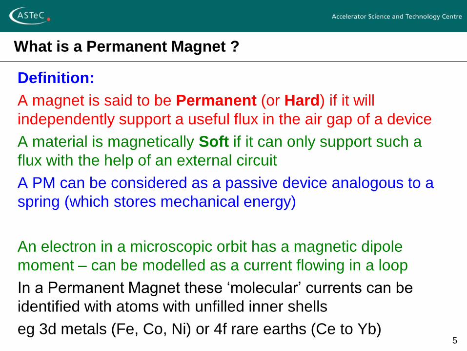
Definition:
A magnet is said to be Permanent (or Hard) if it will
independently support a useful flux in the air gap of a device
A material is magnetically Soft if it can only support such a
flux with the help of an external circuit
A PM can be considered as a passive device analogous to a
spring (which stores mechanical energy)
An electron in a microscopic orbit has a magnetic dipole
moment – can be modelled as a current flowing in a loop
In a Permanent Magnet these ‘molecular’ currents can be
identified with atoms with unfilled inner shells
eg 3d metals (Fe, Co, Ni) or 4f rare earths (Ce to Yb)

6
Permanent Magnets
Permanent Magnet materials are manufactured so that their
magnetic properties are enhanced along a preferred axis
To do this, advantage is taken of crystal lattices
The direction of alignment is called the easy axis
When a magnetic field, B, is applied to a magnetic material
each dipole moment tries to align itself with the field direction
When B is strong enough (at saturation) all of the moments
are aligned, overcoming other atomic forces which resist this
A Permanent Magnet must be able to maintain this
alignment after B is removed

7
An Ideal Permanent Magnet
The characteristics of a Permanent Magnet are determined by
its behaviour under an external magnetization force H
1. H large, material
saturated, all
moments aligned
2. H reducing,
moments stay
aligned
3. H large and negative,
material flips – now
aligned with opposite
direction
Intrinsic coercivity
Magnetization
Magnetizing
Force
Magnetization is magnetic
dipole moment per unit
volume, B = m0M

8
The Ideal BH Curve
Gradient = m0
Remanent Field
Coercivity
In 2nd quadrant the
ideal PM is linear
Magnetic Flux
Density
B = m0(H+M)
Magnetizing
Force

9
The BH Product
Permanent Magnets are operated in the 2nd quadrant – no
external fields are present, moments are aligned along the
easy axis
The product BH represents the energy density of the material
Examining the peak BH value in the 2nd quadrant is a good
way of comparing the strength of different materials
10
The Working Point
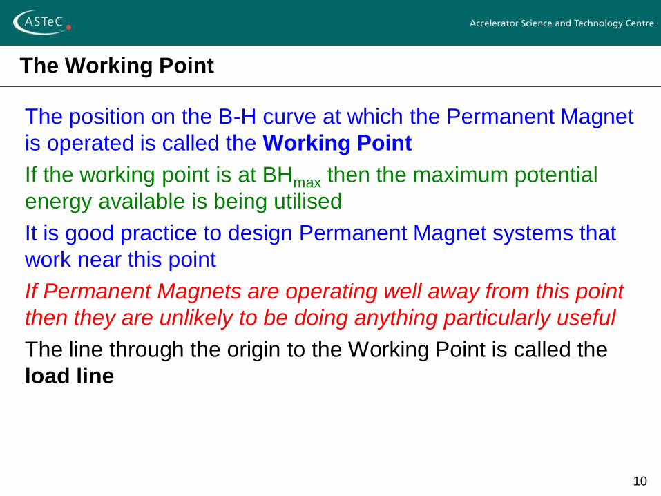
The position on the B-H curve at which the Permanent Magnet
is operated is called the Working Point
If the working point is at BHmax then the maximum potential
energy available is being utilised
It is good practice to design Permanent Magnet systems that
work near this point
If Permanent Magnets are operating well away from this point
then they are unlikely to be doing anything particularly useful
The line through the origin to the Working Point is called the
load line
11
Current Sheet Equivalent Materials (CSEM)
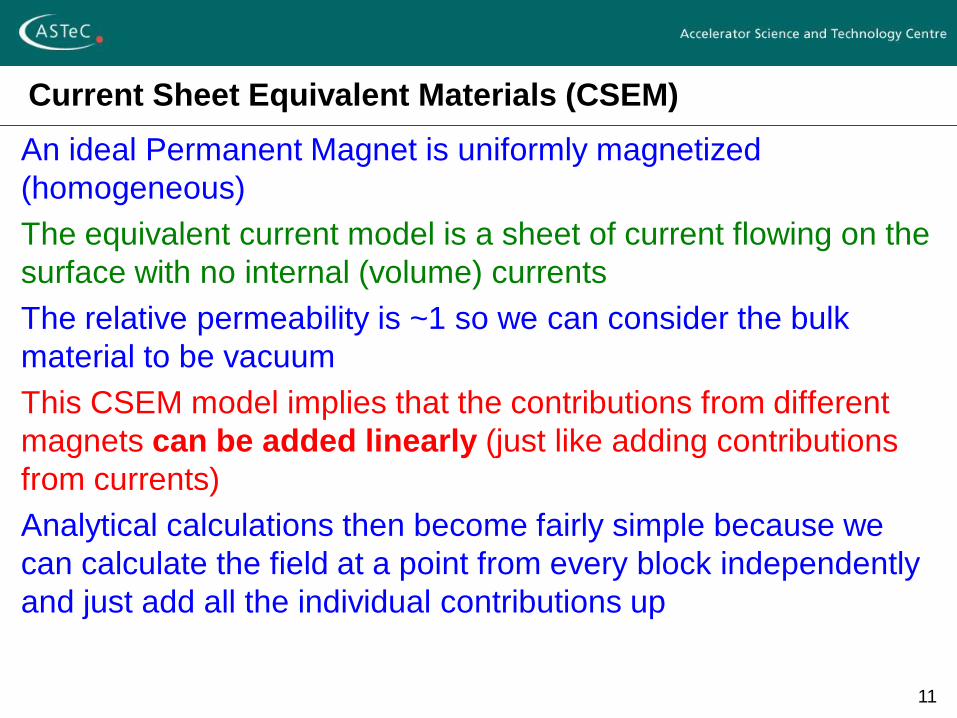
An ideal Permanent Magnet is uniformly magnetized
(homogeneous)
The equivalent current model is a sheet of current flowing on the
surface with no internal (volume) currents
The relative permeability is ~1 so we can consider the bulk
material to be vacuum
This CSEM model implies that the contributions from different
magnets can be added linearly (just like adding contributions
from currents)
Analytical calculations then become fairly simple because we
can calculate the field at a point from every block independently
and just add all the individual contributions up

12
Current Sheet Equivalent Materials (CSEM)
Lines of flux for an
ideal Permanent
Magnet
Lines of flux for a
CSEM model

13
Real Permanent Magnet Materials
Not all materials have a linear BH curve in the 2nd quadrant
This can be a problem if the working point drops into the non-
linear region
This might happen when closing an undulator gap or even
transiently during assembly of the undulator
If the working point moves
from a to b then when B
increases again the magnet
will operate at c instead – this
is an irreversible effect

14
Temperature Effects
At higher temperatures the materials become more non-linear
So long as the working point stays in the linear region this is a
reversible effect
Note that the remanent field drops with increasing temperature
– the reverse is also true, cold magnets have a higher
remanent field
Day to day temperature
variations are important and
must be controlled
(minimised)
Many undulators are
operated in air conditioned
environments to keep their
output more stable
15
Available Materials
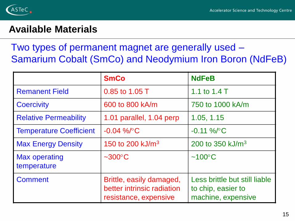
Two types of permanent magnet are generally used –
Samarium Cobalt (SmCo) and Neodymium Iron Boron (NdFeB)
SmCo NdFeB
Remanent Field 0.85 to 1.05 T 1.1 to 1.4 T
Coercivity 600 to 800 kA/m 750 to 1000 kA/m
Relative Permeability 1.01 parallel, 1.04 perp 1.05, 1.15
Temperature Coefficient -0.04 %/C -0.11 %/C
Max Energy Density 150 to 200 kJ/m3 200 to 350 kJ/m3
Max operating
temperature
~300C ~100C
Comment Brittle, easily damaged,
better intrinsic radiation
resistance, expensive
Less brittle but still liable
to chip, easier to
machine, expensive

16
How are Permanent Magnets Manufactured?
Melting of the alloy under
vacuum with inductive heating
Crushing of polycrystalline cast
ingots
Milling of the coarse powder
Pre-alignment in a magnetic field (courtesy of Vacuumschmelze)
17
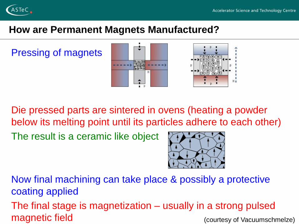
How are Permanent Magnets Manufactured?
Pressing of magnets
Die pressed parts are sintered in ovens (heating a powder
below its melting point until its particles adhere to each other)
The result is a ceramic like object
Now final machining can take place & possibly a protective
coating applied
The final stage is magnetization – usually in a strong pulsed
magnetic field (courtesy of Vacuumschmelze)

18
An Example Material
Vacodym 633 HR
M-H and B-H curves are
shown (2nd quadrant)
The material is linear at
20C but non-linear above
about 60 C
Irreversible losses for
different loadline working
points as a function of
temperature
(courtesy of Vacuumschmelze)
19
Pure Permanent Magnet Undulators
A magnet which contains no iron or current carrying coils is
said to be a Pure Permanent Magnet (PPM)
Because of CSEM we can use the principle of superposition
An ideal undulator would have a sinusoidal magnetic field
along the direction of the electron beam
To generate a sinusoidal field an ideal PPM would have two
sets (arrays) of Permanent Magnet with their easy axis
rotating smoothly through 360 per period along the direction
of the electron beam
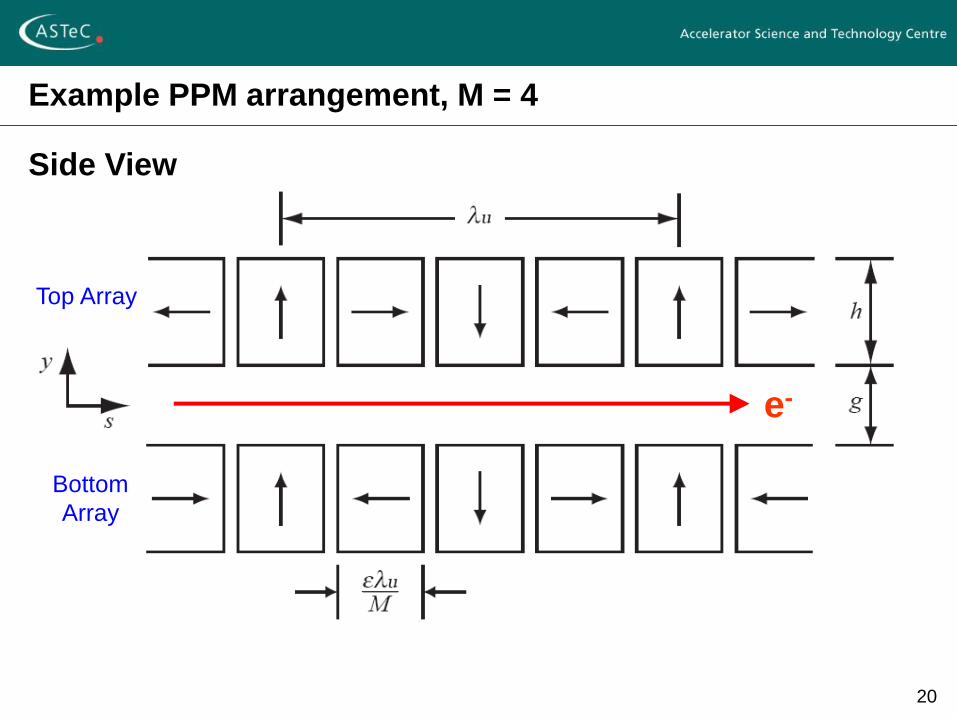
In practice this ideal situation is approximated by splitting the
system into M rectangular magnet blocks per period with the
easy axis at the relevant set angle
20
Example PPM arrangement, M = 4
e-
Side View
Top Array
Bottom
Array

21
Lines of Magnetic Flux
e-

22
Magnetic Field
The field strength between the two arrays assuming infinite
width in the x – direction (2D approximation) is
Where and is a packing factor to allow for small
air gaps between blocks
The vertical field on axis (y = 0) is a number of cosine harmonics
As this reduces to a single cosine (ideal case)
The longitudinal (and horizontal) field on axis is zero

23
A Practical PPM
The most popular choice is M = 4
This is a good compromise between on axis field strength and
quality vs engineering complexity
Higher harmonics then account for < 1% of the field on axis
Away from the axis it is definitely not cosine-like
For an example PPM with
50mm period, block height of
25mm, magnet gap of 20 mm
and remanent field of 1.1 T
Note that the fields increase
away from the axis
24
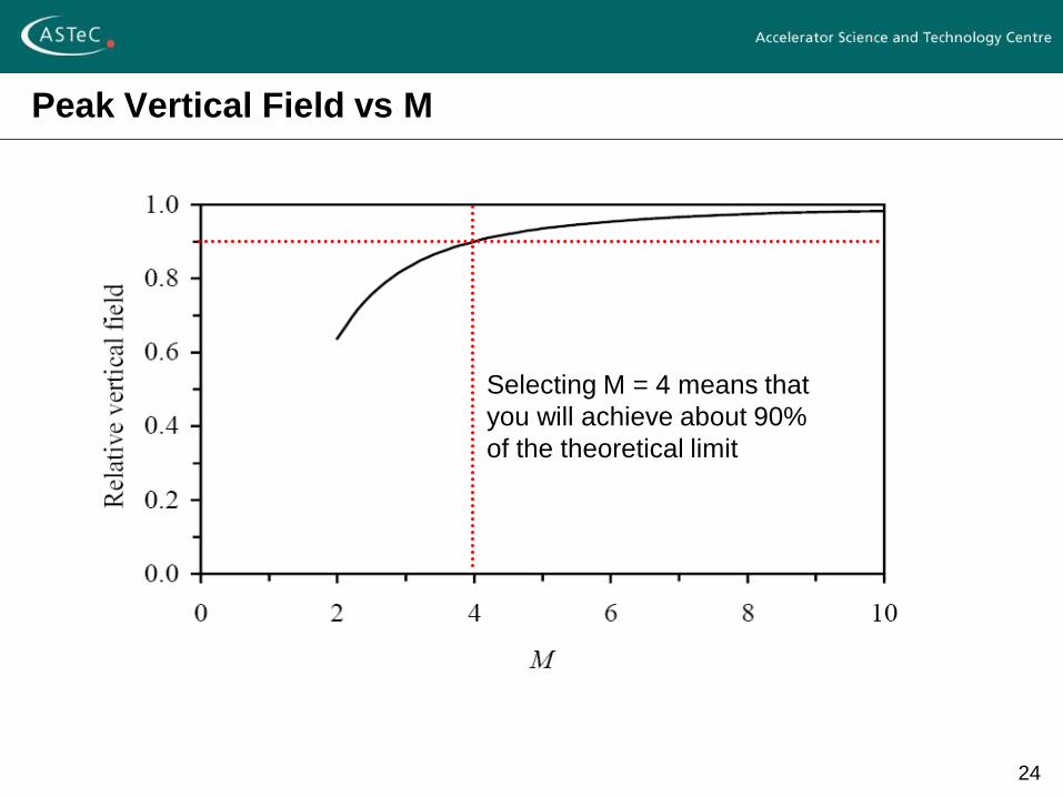
Peak Vertical Field vs M
Selecting M = 4 means that
you will achieve about 90%
of the theoretical limit

25
Simplifying the Magnetic Field
If we assume that only the first harmonic makes a significant contribution (n = 1) – a good approximation in general
Then the equation simplifies greatly on axis to
Important:
Note that so long as all the spatial dimensions scale together the fields on axis do not change
This is not true for electromagnets – there the current densities have to increase to maintain the same field levels

26
Effect of Different Block Heights
A typical block height selection is half the period length
A height of a quarter period length would make all the blocks
identical but then there is a greater field loss
Selecting 0.5 means
that you will achieve
about 95% of the
theoretical limit

27
Peak Field Achievable
The maximum peak field achievable (in theory) is 2Br
In practice with M = 4 and h = lu/2 the peak on axis field is
So even with an ambitious gap to period ratio of 0.1 the peak
value is only 1.26Br
Achieving fields of ~1.5T requires very high Br material, small
gaps and long periods!
But, higher fields are possible if we include iron in the
system
Mixing Permanent Magnets and iron poles is called a hybrid
magnet

28
Tuning the Undulator
To vary the output wavelength from the undulator – to map out
the tuning curves – we need to alter the field level on the axis
We can now see that the only practical way to do this for a
permanent magnet device is to change the magnet gap

29
Hybrid Insertion Devices
Simple hybrid example
Top Array
Bottom
Array
e-

30
Lines of Magnetic Flux
Including a non-linear material like iron means that simple
analytical formulae can no longer be derived – linear
superposition no longer works!
Accurate predictions for particular designs can only be made
using special magnetostatic software in either 2D (fast) or 3D
(slow)
e-
31
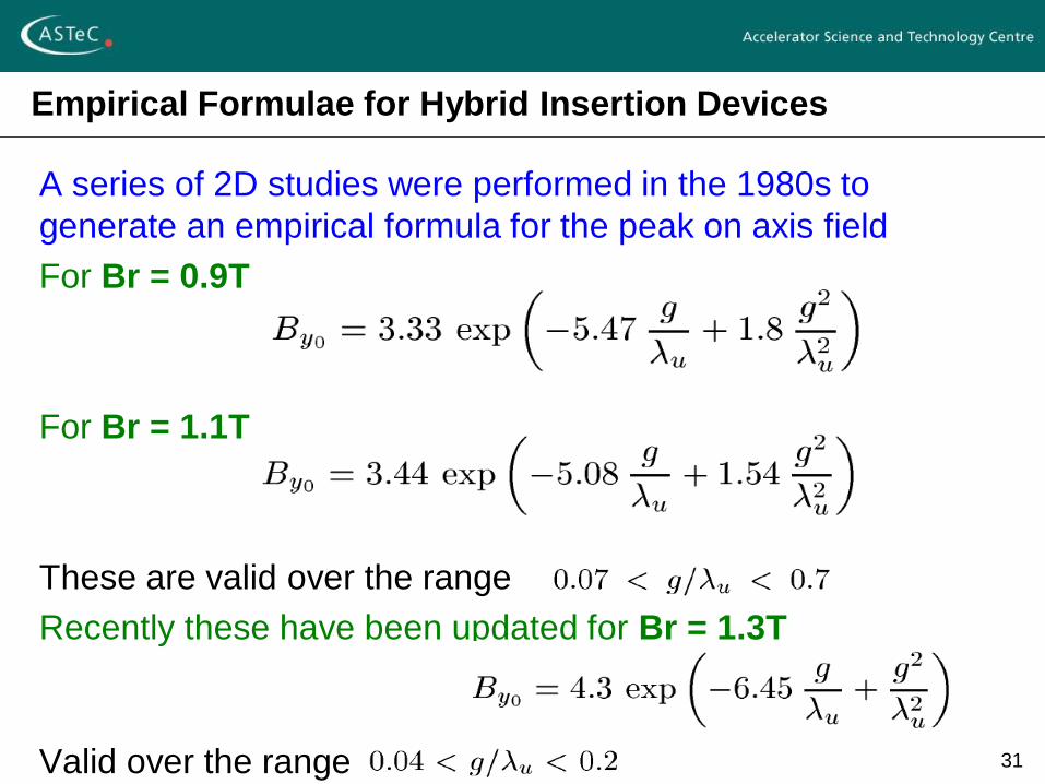
Empirical Formulae for Hybrid Insertion Devices
A series of 2D studies were performed in the 1980s to
generate an empirical formula for the peak on axis field
For Br = 0.9T
For Br = 1.1T
These are valid over the range
Recently these have been updated for Br = 1.3T
Valid over the range

32
Field Levels for Hybrid and PPM Insertion Devices
Assuming Br = 1.1T and gap of 20 mm
When g/lu is
small the impact
of the iron is
very significant

33
Insertion Device End Termination Design
We want undulators and wigglers to have zero net effect on
the electron trajectory
Otherwise, operating one undulator would affect all the other
users
Remember (from Lecture 2)
So, the electron exit angle is found by integrating the field over
the full length of the device
Such that the exit angle, a , is
Iy is called the first field integral
34
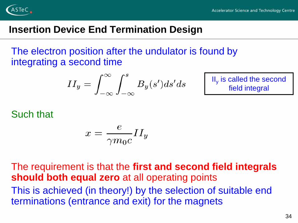
Insertion Device End Termination Design
The electron position after the undulator is found by integrating a second time
Such that
The requirement is that the first and second field integrals should both equal zero at all operating points
This is achieved (in theory!) by the selection of suitable end terminations (entrance and exit) for the magnets
IIy is called the second
field integral

35
Insertion Device End Termination Design
An alternative expression for the final beam position at the exit
is to project it back to the centre of the device
Then
Realistic electron
trajectory in a non-
ideal undulator
36
Symmetric and Antisymmetric Insertion Devices
The parameter d will be zero when the field is symmetric
about s = 0 (centre of the undulator is the peak of a pole)
The end designs then need to be set so that a is also zero
In the antisymmetric case, the centre of the magnet is a zero
crossing
In this case a will automatically be zero
The ends then need to be chosen so that d is also zero
For PPMs the end design is relatively simple because of the
superposition principle
For hybrids the non-linear effects mean that the integrals are
harder to control so active compensation is generally used –
these might be electromagnetic coils or moving permanent
magnets
37
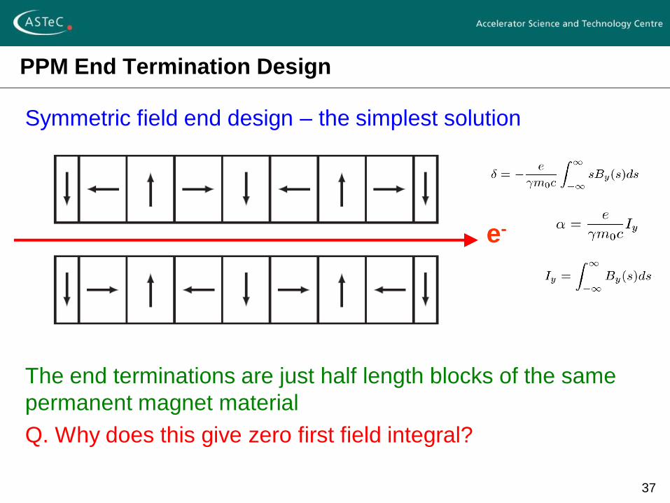
PPM End Termination Design
Symmetric field end design – the simplest solution
The end terminations are just half length blocks of the same
permanent magnet material
Q. Why does this give zero first field integral?
e-

38
PPM End Termination Design
Remember the principle of superposition
e-
The field on-axis
due to this block …
… will be exactly
cancelled by the
field due to this
block
39
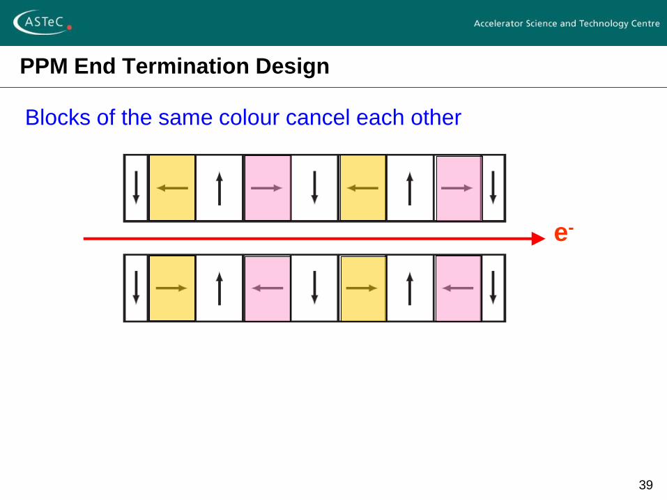
PPM End Termination Design
Blocks of the same colour cancel each other
e-

40
PPM End Termination Design
The same is true for the blocks with vertical easy axis – an ‘up’
block cancels a ‘down’ block
Finally, we are left with two ‘up’ blocks and these are
cancelled by four half length ‘down’ blocks
They have to be half length otherwise the magnet would not
be symmetric and both integrals would not be zero
e-

41
Half Block End Termination Design
10 period model
50 mm period
3GeV trajectory
a and d are zero
Note that there is a
small position offset
through the undulator
but the light is emitted
parallel to the axis
42
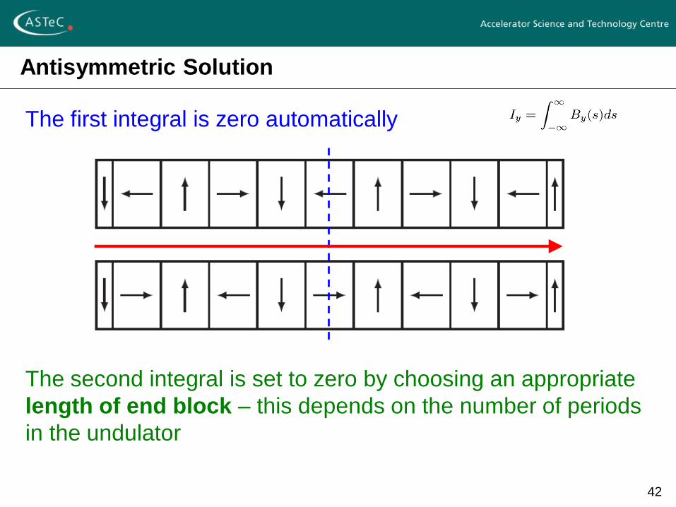
Antisymmetric Solution
The first integral is zero automatically
The second integral is set to zero by choosing an appropriate
length of end block – this depends on the number of periods
in the undulator

43
Antisymmetric Solution
The final position and
angle of the electron are
both zero but the light will
be emitted at an angle to
the axis
10 period model
50 mm period
3GeV trajectory
a and d are zero
44
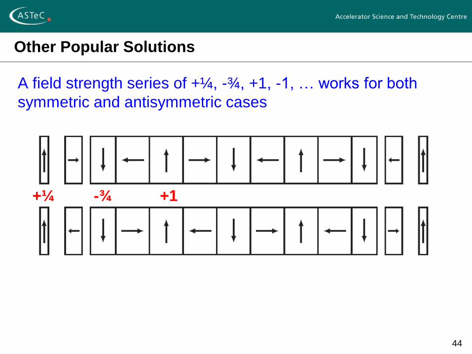
Other Popular Solutions
A field strength series of +¼, -¾, +1, -1, … works for both
symmetric and antisymmetric cases
+¼ -¾ +1

45
The +¼, -¾, +1 Solution
The electron now
oscillates about the axis
so the light will be
emitted along the axis
10 period model
50 mm period
3GeV trajectory
a and d are zero
46
Summary
A Permanent Magnet can independently support a flux in an
air gap – no coils are needed
Permanent Magnets are operated in the 2nd quadrant of the
BH curve – ideally they have a linear behaviour
Permanent Magnets can be modelled as current sheets so we
can add the field contributions from each block linearly
To generate a sinusoidal field we use two arrays of magnet
blocks – one above and one below the electron beam
The field limit is ~1.5T but if we include iron (hybrid magnet)
then >2 T is easily achievable
The end terminations of undulators are important.
The end design can depend on whether the magnet is
symmetric or asymmetric but the design principles are the
same


![Status of In-Vacuum undulators at ESRF · Status of In-Vacuum undulators at ESRF ... Status of in-vacuum undulators SS Period [mm] L [m] ... Rossmanith et al. ANKA/ACCEL PAC03](https://static.cupdf.com/doc/110x72/5bb0193009d3f2e27b8d80e9/status-of-in-vacuum-undulators-at-status-of-in-vacuum-undulators-at-esrf-.jpg)