1
Innovation in Solar Thermal Chimney Power Plants
Patrick John Cottam
A thesis submitted as partial fulfilment of the
requirements for the degree of
Doctor of Engineering
of
University College London
Centre for Urban Sustainability and Resilience
University College London
I, Patrick John Cottam, confirm that the work presented in this thesis is my own.
Where information has been derived from other sources, I confirm that this has been
indicated in the thesis.
____________________________

2
ACKNOWLEDGMENTS
These days, everyone is familiar with predictive text on their mobile phones offering an
occasional insight into their own lives. So it speaks to the steady patience and dedication of
both my supervisors, Dr. Paul Fromme and Dr. Philippe Duffour, that latterly any messages I
write on my phone beginning “Hi,” are predicted to follow with “Paul and Philippe”. Their
support has been infinite and kind. Their technical knowledge has been invaluable. But by
far the greatest lesson I have learned from Paul and Philippe has been how to begin my
research, when in the beginning I knew so little of my field; and how to keep going when
obstacles appeared, as in research they often do. Paul and Philippe deserve my heartfelt
thanks.
I also owe huge thanks to Per Lindstrand and his company Lindstrand Technologies, not
only for working closely with me as project partners throughout, but also for Per’s role as
strategist and promoter, with a long-term vision of what suspended chimneys could be.
Anyone familiar with Per’s extraordinary adventures will know this approach has served him
well. I am also indebted to Lee Barnfield and Stacey Greensall for their technical advice, and
to the team on the shop floor who manufactured my suspended chimney prototypes.
This project has been fortunate enough to receive additional support from the Royal
Commission for the Exhibition of 1851, in the form of their Industrial Fellowship. Their
support and their excellent network of engineers and entrepreneurs has been of great value
to this project, and for that I am very grateful.
My family inform and influence everything I do, and everything I try to be. Mum, Dad, Jack
and Bill influence me for the better in many ways. Thank you, and I look forward to you
scouring this thesis cover-to-cover to find your influence in my work.
Finally, my fiancée, Becky, has been my rock. The support she provided has quite simply
made this possible. Thank you Becky, I love you.

3
ABSTRACT
This thesis analyses novel technology for renewable electricity generation: the solar thermal
chimney (STC) power plant and the suspended chimney (SC) as a plant component. The
STC consists of a solar collector, a tall chimney located at the centre of the collector, and
turbines and generators at the base of the chimney. Air heated in the collector rises up the
chimney under buoyancy and generates power in the turbines. STCs have the potential to
generate large amounts of power, but research is required to improve their economic
viability.
A state-of-the-art STC model was developed, focussing on accurate simulation of collector
thermodynamics, and providing data on flow characteristics and plant performance. It was
used to explore power generation for matched component dimensions, where for given
chimney heights, a range of chimney and collector radii were investigated. Matched
dimensions are driven by the collector thermal components approaching thermal equilibrium.
This analysis was complemented with a simple cost model to identify the most cost-effective
STC configurations. The collector canopy is an exceptionally large structure. Many of the
designs proposed in the literature are either complex to manufacture or limit performance.
This thesis presents and analyses a series of novel canopy profiles which are easier to
manufacture and can be incorporated with little loss in performance.
STC chimneys are exceptionally tall slender structures and supporting their self-weight is
difficult. This thesis proposes to re-design the chimney as a fabric structure, held aloft with
lighter-than-air gas. The performance of initial, small scale suspended chimney prototypes
under lateral loading was investigated experimentally to assess the response to wind loads.
A novel method of stiffening is proposed and design of larger prototypes developed. The
economic viability of a commercial-scale suspended chimney was investigated, yielding cost
reductions compared to conventional chimney designs.

4
TABLE OF CONTENTS
1 Introduction .................................................................................................................................. 15
2 Solar Thermal Chimneys: Literature Review and Motivation ............................................... 18
2.1 STCs: History and Context ............................................................................................... 18
2.2 The Manzanares STC Plant ............................................................................................. 19
2.3 Overview of STC Literature .............................................................................................. 22
2.4 Simplified Mathematical Models ...................................................................................... 23
2.5 Comprehensive Mathematical Models ............................................................................ 26
2.6 CFD Models ........................................................................................................................ 31
2.7 Physical Experiments ........................................................................................................ 36
2.8 Optimisation ........................................................................................................................ 39
2.9 STC Cost Modelling ........................................................................................................... 40
2.10 STC Heat & Power Management .................................................................................... 42
2.11 Sloped-Collector STCs ...................................................................................................... 43
2.12 Collector Canopy Profiles.................................................................................................. 45
2.13 STC System Sizing ............................................................................................................ 46
2.14 STC Literature Summary .................................................................................................. 47
3 Solar Thermal Chimneys: Modelling ........................................................................................ 48
3.1 Simple Analytical Model .................................................................................................... 49
3.2 Comprehensive Model Overview ..................................................................................... 55
3.3 Comprehensive Analytical Model Structure ................................................................... 56
3.4 Collector Governing Equations ........................................................................................ 57
3.5 Collector Discretisation ...................................................................................................... 60
3.6 Collector Thermal Network ............................................................................................... 61
3.7 Heat Transfer Coefficients ................................................................................................ 64
3.8 Collector Air Flow ............................................................................................................... 70
3.9 Surface Shear Stress ......................................................................................................... 71
3.10 Collector-to-Chimney Transition Section ........................................................................ 73
3.11 Chimney Model ................................................................................................................... 75
3.12 Turbine Model ..................................................................................................................... 79
3.13 Comprehensive Analytical Model Structure ................................................................... 80
3.14 STC Model Validation ........................................................................................................ 80
3.15 STC Numerical Coherence Checks ................................................................................ 82
4 Solar Thermal Chimneys: Parametric Investigations ............................................................ 83
4.1 STC Air-Surface Friction ................................................................................................... 85
5
4.2 Optimum Turbine Pressure Drop Ratio .......................................................................... 89
4.3 STC Sensitivity Analysis.................................................................................................... 94
4.4 Dimension Matching .......................................................................................................... 99
4.5 Conclusions ....................................................................................................................... 110
5 Solar Thermal Chimneys: Design for Construction ............................................................. 113
5.1 Exponential Canopy Profile ............................................................................................ 115
5.2 Flat Canopy Profile ........................................................................................................... 118
5.3 Constant-Gradient Sloped Canopy Profile ................................................................... 120
5.4 Segmented Canopy Profile ............................................................................................. 123
5.5 Stepped Canopy Profile .................................................................................................. 126
5.6 Optimum Rgrad Sensitivity to Plant Dimensions ............................................................ 127
5.7 Air Flow Properties ........................................................................................................... 129
5.8 Air Properties at the Chimney Inlet ................................................................................ 131
5.9 Conclusions ....................................................................................................................... 132
6 Suspended Chimneys: Literature Review and Motivation ................................................. 134
6.1 Solar Thermal Chimney Power Plants – Chimney Construction & Analysis ........... 134
6.2 Wind Loading on Chimney Structures .......................................................................... 139
6.3 Modelling of Inflated Beams ........................................................................................... 140
6.4 Experimental Testing of Inflatable Beams .................................................................... 144
6.5 Inflatable Structures Under Wind Loading .................................................................... 145
6.6 Industrial Fabrics .............................................................................................................. 146
6.7 Summary ........................................................................................................................... 147
7 Suspended Chimneys: Design Development ...................................................................... 148
7.1 Inflatable Structures – State-of-the-Art ......................................................................... 149
7.2 SC1 Prototype ................................................................................................................... 150
7.3 SC2 Prototype ................................................................................................................... 157
7.4 SC3 Prototype ................................................................................................................... 164
7.5 SC4 Prototype ................................................................................................................... 167
7.6 Further SC Prototypes ..................................................................................................... 168
7.7 Conclusions ....................................................................................................................... 170
8 Suspended Chimneys: Data Analysis ................................................................................... 173
8.1 Experimental Method ....................................................................................................... 174
8.2 SC2 Prototype ................................................................................................................... 177
8.3 SC3-1 Prototype ............................................................................................................... 181
8.4 SC3-2 Prototype ............................................................................................................... 184
8.5 Summary & Conclusions ................................................................................................. 188

6
9 Suspended Chimneys: Commercialisation ........................................................................... 190
9.1 Market Opportunity ........................................................................................................... 190
9.2 Suspended Chimney Prototypes ................................................................................... 192
9.3 Suspended Chimneys and the Solar Thermal Chimney Power Plant...................... 198
9.4 Concluding Remarks ....................................................................................................... 200
10 Conclusions ............................................................................................................................... 202
10.1 Solar Thermal Chimneys: Literature Review ............................................................... 202
10.2 Solar Thermal Chimneys: Modelling ............................................................................. 202
10.3 Solar Thermal Chimneys: Parametric Investigations .................................................. 203
10.4 Solar Thermal Chimneys: Design for Construction ..................................................... 203
10.5 Suspended Chimneys: Literature Review .................................................................... 204
10.6 Suspended Chimneys: Design Development .............................................................. 205
10.7 Suspended Chimneys: Data Analysis ........................................................................... 206
10.8 Suspended Chimneys: Commercialisation .................................................................. 207
10.9 Concluding Remarks ....................................................................................................... 207
11 References ................................................................................................................................ 208
I. Appendix: Reference STC Properties ................................................................................... 218
II. Appendix: STC Numerical Checks ........................................................................................ 220
III. Appendix: Suspended Chimney Design Options for SC1 .................................................. 223
SC1 Dimensioning ....................................................................................................................... 223
SC1 Design Options .................................................................................................................... 224
IV. Appendix: Suspended Chimney Design Parameters .......................................................... 230
V. Appendix: Derivation of SC2 Dimensioning Equation......................................................... 231
VI. Appendix: Suspended Chimney Design Drawings – 20 m Tall ......................................... 234
VII. Appendix: SC2 Prototype Design .......................................................................................... 237
VIII. Appendix: SC Prototypes – 20 m Tall – Design Options .................................................... 238
IX. Appendix: Identifying Potential Customers ........................................................................... 240
Favourable Geographical Regions ............................................................................................ 240
Characterisation of Potential Customers .................................................................................. 241
X. Appendix: Commercial Suspended Chimney Costs ........................................................... 243
XI. Appendix: Route to Commercialisation ................................................................................. 245
Hire of Suspended Chimneys ..................................................................................................... 246

7
TABLE OF FIGURES
Figure 1.1. A diagram of the solar thermal chimney (STC) concept. .................................... 15
Figure 2.1. Schematic of the solar thermal chimney power plant. ........................................ 19
Figure 2.2. A model of the automatic roasting spit (Museum for the History of Science &
Technology in Islam, Istanbul, Turkey). ...................................................................... 19
Figure 2.3. The Motor Solar designed by Cabanyes [45]. .................................................... 19
Figure 2.4. An aerial photograph of the Manzanares research prototype STC [45]. ............ 20
Figure 2.5. The Solar Thermal Chimney as studied by Padki & Sherif [13] .......................... 25
Figure 2.6. Transpired solar collector compared to "conventional" STC collector. Note that
the periphery of the transpired collector is enclosed [70]. ........................................... 38
Figure 2.7. Sloped STC concept [88]. ................................................................................. 43
Figure 3.1. Schematic of the solar thermal chimney power plant. ........................................ 48
Figure 3.2. Dimensions and air properties at the collector-to-chimney transition section. .... 51
Figure 3.3. Power output and collector temperature rise for a range of chimney heights
simulated by the simple STC model. .......................................................................... 53
Figure 3.4. Power output and collector temperature rise for a range of collector radii
simulated by the simple STC model. .......................................................................... 53
Figure 3.5. Dependence of STC power output and collector air temperature rise upon
collector thermal efficiency. ........................................................................................ 54
Figure 3.6. Power output and collector air temperature rise for varying turbine to chimney
pressure drop ratio, simple STC model. ..................................................................... 54
Figure 3.7. Interdependent STC operating processes ......................................................... 57
Figure 3.8. A collector section with thermal components and heat flows ............................. 58
Figure 3.9. Discretised collector annuli. ............................................................................... 61
Figure 3.10. Power output for reference STC with reference environmental conditions and
varying quantity of discretised elements in collector. .................................................. 61
Figure 3.11. A schematic diagram of the collector-to-chimney flow section demonstrating the
input and output flow variables. .................................................................................. 73
Figure 3.12. STC model & sub-model hierarchy .................................................................. 81
Figure 4.1. Normalised power output for varying roughness lengths: (a) canopy roughness
length; (b) ground roughness length; (c) chimney internal surface roughness length.
Reference STC dimensions and ambient conditions (I = 900 Wm-2; T∞ = 305 K). ....... 87
Figure 4.2. Collector air temperature change and collector air pressure change (modulus
values) for varying ground roughness length. Assumes constant mass flow rate of m =
1.6648 × 10⁵kgs-1 with reference collector dimensions. ............................................. 88
8
Figure 4.3. Power output produced by reference STC (Hci = 4.0 m, Hco = 11.5 m) under
reference conditions with a range of turbine pressure drop ratio values. .................... 89
Figure 4.4. STC performance for varying values of turbine pressure drop ratio and insolation.
.................................................................................................................................. 90
Figure 4.5. STC performance for varying values of turbine pressure drop ratio and ambient
temperature. .............................................................................................................. 90
Figure 4.6. STC performance for varying values of turbine pressure drop ratio and collector
radius. ........................................................................................................................ 90
Figure 4.7. STC performance for varying values of turbine pressure drop ratio and chimney
height. ........................................................................................................................ 92
Figure 4.8. STC performance for varying values of turbine pressure drop ratio and chimney
radius. ........................................................................................................................ 92
Figure 4.9. Rate of heat flux radiated from canopy surface to the sky for changing ambient
air temperature. Assumes a constant temperature difference between ambient air and
canopy surface. ......................................................................................................... 95
Figure 4.10. STC power output profiles in response to varying environmental parameters: (a)
impact of changing insolation on STC power output; (b) impact of changing ambient
temperature on STC power output; (c) impact of ambient wind velocity (above collector
canopy only) on STC power output. Reference STC dimensions and environmental
parameters. ................................................................................................................ 96
Figure 4.11. STC power output profiles in response to varying STC component parameters:
(a) impact of collector radius size; (b) impact of chimney radius size; (c) impact of
chimney height. Reference STC dimensions and environmental parameters. ............ 98
Figure 4.12. Power output for STCs with varying collector canopy outlet height and chimney
radius. Rc = 5500 m, Hch = 1000 m, Hci = 4 m, I = 900 Wm-2, T∞ = 305 K. ................. 100
Figure 4.13. STC power output for varying combinations of chimney radius and collector
radius. Hci = 4 m; Hco = 24 m; I = 900 Wm-2; T∞ = 305 K. .......................................... 103
Figure 4.14. Collector component temperatures for STCs with different sizes of solar
collector. Dotted lines represent ground temperatures; dashed lines represent canopy
temperatures and solid lines represent working air temperatures. Hch = 1000 m, Hco =
20 m, I = 900 Wm-2, T∞ = 305 K................................................................................ 104
Figure 4.15. Effect of chimney radius on flow parameters: (a) Chimney inlet pressure
potential; (b) system mass flow rate; (c) product of pressure potential and mass flow
rate. Rc = 3000 m; Hch = 1000 m; Hci = 4 m; Hco = 16 m; I = 900 Wm-2; T∞ = 305 K. . 105
Figure 4.16. Change in power output with respect to change in collector size for a range of
STC configurations. Hci = 4 m; Hco = 24 m; I = 900 Wm-2; T∞ = 305 K. ...................... 106
9
Figure 4.17. Power output per unit cost for Scenario 3 costs (wherein the chimney and
turbine have double the relative cost compared to the collector than that specified by
Fluri et al.) ................................................................................................................ 107
Figure 4.18. Power output per unit cost for STCs with varying collector area and chimney
flow area. (a) chimney height = 500 m; (b) chimney height = 750 m; (c) chimney height
= 1000 m. Hci = 4 m; Hco = 24 m; I = 900 Wm-2; T∞ = 305 K. ..................................... 109
Figure 4.19. STC power output for a limited range of collector surface areas and chimney
radii, with the cold air inflow (CAI) boundary included. All configurations below the CAI
boundary are unlikely to suffer power loss due to cold air inflow. Hci = 4 m; Hco = 24 m;
I = 900 Wm-2; T∞ = 305 K. ........................................................................................ 110
Figure 5.1. Different STC canopy profile options: (a) exponential profile; (b) flat profile; (c)
constant-gradient sloped profile; (d) segmented sloped profile; (e) segmented stepped
profile. ...................................................................................................................... 115
Figure 5.2. Change in power output with canopy exponent for the reference STC with an
exponential canopy. Canopy outlet height given for reference (Hci = 4 m, I = 900 Wm-2,
T∞ = 305 K). ............................................................................................................. 116
Figure 5.3. Change in power output for the reference STC with a flat canopy of varying
height (I = 900 Wm-2, T∞ = 305 K). ........................................................................... 119
Figure 5.4. Change in power output for a reference STC with a sloped canopy with varying
canopy outlet height (Hci = 4 m, I = 900 Wm-2, T∞ = 305 K). ..................................... 120
Figure 5.5. Air velocity through a collector of reference dimensions with a constant-gradient
sloping canopy. Seven cases are presented with canopy outlet height ranging from 4
m to 100 m (Hci = 4 m, I = 900 Wm-2, T∞ = 305 K). ................................................... 121
Figure 5.6. Power output for reference STC with constant-gradient canopy and changing
canopy outlet height, simulated for varying insolation. Hci = 4 m; T∞ = 305 K; Rc = 2150
m; Hch = 1000 m; Rc = 55 m. .................................................................................... 123
Figure 5.7. Power output for reference STC with constant-gradient canopy and changing
canopy outlet height, simulated for varying ambient temperature. Hci = 4 m; I = 900
Wm-2; Rc = 2150 m; Hch = 1000 m; Rc = 55 m. .......................................................... 123
Figure 5.8. Change in power output for a reference STC with a segmented canopy profile
(Hci = 4 m, I = 900 Wm-2, T∞ = 305 K). ...................................................................... 124
Figure 5.9. STC performance for varying values of rgrad under different levels of insolation. T∞
= 305 K, Rc = 2150 m, Hch = 1000 m, Hci = 4 m, Hco = 12.25 m. ............................... 125
Figure 5.10. STC performance for varying values of rgrad and different ambient temperatures.
I = 900 Wm-2; Rc = 2150 m; Hch = 1000 m; Hci = 4 m; Hco = 12.25 m. ........................ 125

10
Figure 5.11. Performance of the reference STC with a collector of varying radius Rc and
varying change-of-gradient point rgrad, which is normalised against Rc on the x-axis. I =
900 Wm-2; T∞ = 305K; Hch = 1000m; Hci = 3m; Hco = 7m. .......................................... 128
Figure 5.12. Performance of the reference STC with a chimney of varying height Hch and
varying change-of-gradient point rgrad. I = 900 Wm-2; T∞ = 305K; Rc = 2150m; Hci = 3m;
Hco = 7m. .................................................................................................................. 128
Figure 5.13. Air temperature profile through the STC collector with different canopy
configurations. Reference STC dimensions and ambient conditions. ....................... 129
Figure 5.14. Air velocity profile for the best-performing configuration of each type of collector
canopy studied. Reference STC dimensions and ambient conditions. ..................... 130
Figure 5.15. Static air pressure profiles through the last 800 m of collector radial path, for the
best-performing configurations of all canopy types. Reference STC dimensions and
ambient conditions. .................................................................................................. 130
Figure 5.16. Working air mean velocity and pressure difference between ambient and
working air at chimney inlet for: (a) the exponential canopy profile; (b) the flat canopy
profile; (c) the sloped canopy profile; and (d) the segmented canopy profile. Reference
STC dimensions and environmental conditions. Hci = 4m unless otherwise specified.
................................................................................................................................ 132
Figure 6.1. Diameter and wall thickness of proposed chimney design for a solar thermal
chimney power plant [1]. .......................................................................................... 135
Figure 6.2. Distribution of meridional forces in the chimney circumference for varying ring
stiffness (taken at 280 m height), as produced by Harte et al. [1]. ............................ 136
Figure 6.3. Design details of proposed floating chimney design [119]. .............................. 137
Figure 6.4. Floating solar chimney schematic showing proposed hinged base [120] ......... 138
Figure 6.5. Pressure coefficient profile around chimney circumference for varying flow
conditions [113] . ...................................................................................................... 140
Figure 6.6. Three-point loading of a simply-supported inflated beam with custom supports to
prevent asymmetrical loading of beam cross-section [130]. ..................................... 145
Figure 6.7. Bi-axial material testing of Octax-835 by manufacturers aeroix GmbH. Stress-
strain data obtained according to ISO 1394-1 at 20 mm/min. Different colours
represent repeated experiments. [149]. .................................................................... 146
Figure 7.1. A computer-generated image demonstrating the suspended chimney concept.
................................................................................................................................ 148
Figure 7.2. A computer-generated image showing the suspended chimney from above. .. 149
Figure 7.3. Octax material on the vacuum CNC cutting table at Lindstrand Technologies Ltd,
cutting patterns for SC1 manufacture. ...................................................................... 152
11
Figure 7.4. The completed SC1 prototype inflated with helium at Lindstrand Technologies'
premises. ................................................................................................................. 152
Figure 7.5. Helium supply valve and tubing causing a point-load deflection and deformation
of a torus on the SC1. .............................................................................................. 152
Figure 7.6. Deflection (x-direction) of the left and right side of the upper and lower tori under
progressively increasing load. .................................................................................. 154
Figure 7.7. Torus rotation under load. Note the initial non-zero rotation due to the structure
listing under the point-mass load of the helium supply valves. ................................. 154
Figure 7.8. SC1 loaded at F=9.8N ..................................................................................... 154
Figure 7.9. Horizontal deformation (change in diameter of outer edges) of SC1 tori under
load. ......................................................................................................................... 155
Figure 7.10. Suspended chimney deflection in the wind. ................................................... 156
Figure 7.11. Suspended chimney using the proposed design, with thin high-pressure inner
and outer sheathes. Chimney shown has been dimensioned for an internal flow
diameter of 1.0 m and a height of 20.0 m in two modules. ....................................... 158
Figure 7.12. SC2 concept diagram showing the key dimensions of one cell wall cross-
section, enclosing an internal flow area of radius r1. ................................................. 159
Figure 7.13. Relationship between external (total) chimney diameter and internal chimney
flow diameter for the SC2 design. ............................................................................ 160
Figure 7.14. Chimney external diameter and chimney section mass for different specific
masses of air-tight and helium-tight fabrics. ............................................................. 161
Figure 7.15. SC2 air-pressurised suspended chimney prototype at Lindstrand Technologies'
manufacturing facilities............................................................................................. 162
Figure 7.16. SC2 manufacturing method. Diagram shows a cross-sectional view of the SC2
wall. Red hatched areas represent joins using glue, welding, stitching and fabric tape.
................................................................................................................................ 162
Figure 7.17. Ovalisation visible on the SC2 loaded at the topmost eyelet. p = 10 kPa; F =
225 N. ...................................................................................................................... 163
Figure 7.18. Torn threads between cells in the SC2 suspended chimney prototype (image
taken with SC2 partially deflated). ............................................................................ 163
Figure 7.19. SC3 - two modules joined and secured to the ground, ready for lateral loading
experiments. ............................................................................................................ 165
Figure 7.20. Lacing detail between the modules of the SC3 suspended chimney prototype.
................................................................................................................................ 165
Figure 7.21. Schematic of SC3 cross-section, with welds shown in cross-hatched red. Each
cell can rotate relative to its neighbours, meaning that the inflated structure does not
form a circular cross-section without additional support. .......................................... 165
12
Figure 7.22. Both modules of the SC3 prototype loaded at the tip, demonstrating the action
of the laced joint as a stiff hinge. p = 30 kPa; F = 172 N. .......................................... 166
Figure 7.23. SC3 strengthening modifications. (a) plastic hoops to strengthen the joint
between the modules; and (b) a wooden platform installed to raise the base of the
fabric and increase the tension applied to secure the structure. ............................... 167
Figure 7.24. SC3 prototype with cross-sectional reinforcement (plastic hoops), joint
reinforcement and base reinforcement. .................................................................... 167
Figure 7.25. SC4 assembled with two modules laced together. SC3 can be seen partially
deflated on the testing rig. ........................................................................................ 168
Figure 7.26. Design A cost breakdown - 20 m tall helium-supported SC with pressurised air-
filled sheathes for lateral stiffness. ........................................................................... 169
Figure 7.27. Design C cost breakdown - 20 m tall SC consisting of an air-filled wall only. . 170
Figure 8.1. Diagram of experimental equipment for testing the deflection of SC2, SC3-1 and
SC3-2. A digital camera takes pictures of the deflected structure to record the location
of the dots. ............................................................................................................... 173
Figure 8.2. SC2 with coloured dots for deflection tracking, loaded with a loop wrapped
around the tip. P = 40 kPa; F = 323 N. SC3-1 can be seen in the background awaiting
testing. ..................................................................................................................... 174
Figure 8.3. Lateral deflection shapes of SC2 under eight load cases for three internal
pressures, with rotational-spring correction. ............................................................. 177
Figure 8.4. Wrinkling evident in the SC2 at 10 kPa loaded with 374 N. ............................. 178
Figure 8.5. Lateral deflection of SC2 tip for varying load and internal pressure. ................ 179
Figure 8.6. Bending stiffness (Euler-Bernoulli beam model) of the SC2 prototype for different
internal pressures. Stiffness values were calculated at F = 342 N. ........................... 179
Figure 8.7. Experimental and Euler-Bernoulli model beam deflections for SC2. Experimental
observed deflection shapes are in blue, modelled deflection shapes are in red. ...... 180
Figure 8.8. Deflection shapes of SC3-1 at internal pressures of 10 kPa, 30 kPa and 50 kPa,
for a range of lateral tip loads. .................................................................................. 182
Figure 8.9. SC3-1 deflection of neutral axis tip under increasing tip load, for a range of
inflation pressures, corrected for rotation of the base. .............................................. 182
Figure 8.10. SC3-1 prototype with wrinkling occurring close to the base. p = 10 kPa, F = 238
N. ............................................................................................................................. 183
Figure 8.11. SC2 (solid line) and SC3-1 (dashed line) bending stiffness for varying internal
pressure, based on Euler Bernoulli (all data recorded at F = 337 N). ....................... 183
Figure 8.12. Comparison of SC2 (solid line) and SC3-1 (dashed line) tip deflection under
load for varying internal pressure. ............................................................................ 184

13
Figure 8.13. SC3-2 inflated to 50 kPa and loaded with 108 N at the tip. Internal stiffening
hoops and additional hoops for strengthening the joint between modules have been
installed. .................................................................................................................. 185
Figure 8.14. SC3-2 neutral axis deflection shapes under various tip loads. ....................... 185
Figure 8.15. SC3-2 tip deflections for varying internal pressure and tip load. Dashed lines
represent inaccurate data due to prototype behaving as a string between ground
connection and pulley. ............................................................................................. 186
Figure 8.16. SC3-2 inflated to 20 kPa, loaded with 194 N. ................................................ 186
Figure 8.17. Bending stiffness of SC2 (solid line), SC3-1 (dashed line) and SC3-2 (dotted
dashed line) based on Euler-Bernoulli model for varying internal pressures. SC2 &
SC3-1 recorded at 337 N; SC3-2 recorded at F = 197 N. ......................................... 187
Figure 9.1. Slip-forming construction of natural-draft cooling tower [154] .......................... 191
Figure 9.2. Suspended chimney prototype 1 (SC1) under test in UCL Mechanical
Engineering laboratories .......................................................................................... 193
Figure 9.3. SC1 Cost breakdown. ..................................................................................... 193
Figure 9.4. Project cost breakdown of SC5 ....................................................................... 195
Figure 9.5. 10m tall module of the proposed SC5 prototype. The prototype will consist of two
such modules. .......................................................................................................... 196
Figure 9.6. Cost breakdown of STC structure with concrete or suspended chimneys. ...... 199
Figure III.1. Change in surface area and enclosed volume for a single torus with varying
small radius. Large radius fixed at R = 1.00 m. ........................................................ 224
Figure III.2. Cross-sectional profile of SC1A module, consisting of two stacked tori, of which
only the top torus is supplied with helium, while the lower torus contains pressurised
air. ........................................................................................................................... 226
Figure III.3. Cross-section profile of SC1B module with double fabric curtains between tori.
................................................................................................................................ 227
Figure III.4. Cross-sectional profile of SC1C design option with a single fabric curtain
between tori. ............................................................................................................ 227
Figure IX.1. Seismically active locations [153]. .................................................................. 240
14
TABLE OF TABLES
Table 2.1. Key dimensions and materials used in the Manzanares STC [3]. ....................... 20
Table 3.1. STC model performance – comparison. ............................................................. 82
Table 4.1. Natural surface roughness lengths extracted by Kröger [108]............................. 85
Table 4.2. Temperature change required to achieve a density difference of 0.05 kgm-3 for
varying initial ambient temperature, according to the Boussinesq approximation. .... 97
Table 4.3. Non-dimensional specific cost for STC cost constraints in optimisation process.
Normalised at collector cost = 1 unit per m2. .......................................................... 106
Table 4.4. Sensitivity analysis of optimal dimensions for different ratios of component unit
costs. All costs are given relative to the collector, which has a specific cost of 1
unit/m2 of collector area. ....................................................................................... 108
Table 6.1. Lamcotec SFO-5951-1 fabric properties (data produced from tests carried out by
Lindstrand Technologies Ltd). ................................................................................ 146
Table 8.1. FujiFilm X-T10 camera properties. ................................................................... 174
Table 9.1. Conventional chimneys vs. suspended chimneys. ............................................ 192
Table 9.2. SC1 technical specifications ............................................................................. 193
Table 9.3. Key technical specifications of the SC5 ............................................................ 196
Table 9.4. Projected costs of commercial-scale suspended chimney products. ................ 197
Table 9.5. Solar thermal chimney power plant key dimensions ......................................... 199
Table 9.6. Key performance metrics of STCs with concrete or suspended chimneys ........ 199
Table I.1. Reference STC collector properties. .................................................................. 218
Table I.2. Reference STC chimney properties. .................................................................. 218
Table I.3. Reference STC turbine & powerblock properties. .............................................. 218
Table I.4. STC reference environmental properties. Values labelled (a) obtained from
Bernardes et al. (2003); values labelled (b) obtained from Pretorius & Kröger (2006).
.............................................................................................................................. 219
Table II.1. Model parameters (convergence criteria, assumed values, etc.) ...................... 221
Table II.2. STC model sensitivity against system parameters. ........................................... 222
Table III.1. Properties common to all SC1 design options. ................................................ 225
Table III.2. Dimensions and material consumption per module for all SC1 design options. 228
Table III.3. SC1 design options - total chimney external dimensions. ................................ 229
Table IV.1. Suspended chimney parameters. .................................................................... 230
Table X.1. Forecast commercial-scale suspended chimney dimensions and costs
(comprehensive version)........................................................................................ 244
Table XI.1. SC route to commercialisation - Stages 1 - 4. ................................................. 248
Table XI.2. SC route to commercialisation - Stages 5 - 8. ................................................. 249
15
1 INTRODUCTION
As the world transitions away from fossil fuels, research into different kinds of renewable
energy technologies is advancing quickly. Of the renewable energy sources available, solar
power is one of the most promising. A variety of technologies have been proposed to
harness this energy and transform it into the electricity upon which we depend. Some have
achieved greater levels of commercial success, thus far, than others.
Research and development of renewable energy technologies is acknowledged to be vital. A
range of energy sources would benefit from further research. The solar thermal chimney
power plant (STC) offers a way to generate large amounts of electrical power from solar
energy. Also sometimes called a solar updraft tower, the STC is a large scale solar power
plant suited for desert deployment. It consists of a solar collector, which generates buoyant
air; a tall chimney through which the buoyant air rises; and a turbine and generator set which
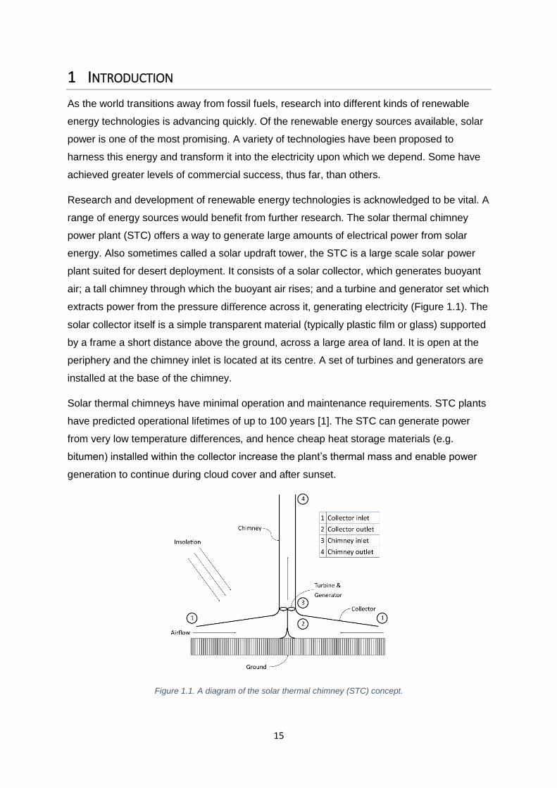
extracts power from the pressure difference across it, generating electricity (Figure 1.1). The
solar collector itself is a simple transparent material (typically plastic film or glass) supported
by a frame a short distance above the ground, across a large area of land. It is open at the
periphery and the chimney inlet is located at its centre. A set of turbines and generators are
installed at the base of the chimney.
Solar thermal chimneys have minimal operation and maintenance requirements. STC plants
have predicted operational lifetimes of up to 100 years [1]. The STC can generate power
from very low temperature differences, and hence cheap heat storage materials (e.g.
bitumen) installed within the collector increase the plant’s thermal mass and enable power
generation to continue during cloud cover and after sunset.
Figure 1.1. A diagram of the solar thermal chimney (STC) concept.
16
As simple base-load power generators, solar thermal chimneys are worthy of research
attention to push the technology towards commercial viability.
Solar thermal chimneys require a tall chimney and a large collector. Many researchers have
studied STC configurations with chimneys of 1000 m tall or taller, and collectors more than 3
km across (e.g. [2]–[5]). The size of the chimney presents novel technological challenges. A
slender thin-shell structure of such height encounters problems resisting wind loading and
problems concerning its own structural stability. Further research is required to transition this
from concept to readiness for construction. The solar thermal chimney is an attractive
concept for solar power generation. However, issues concerning ease of construction - due
to its scale - and technical risk - due to the tall, slender, thin-walled chimney – are limiting the
progress of commercial STC projects.
The present work addresses these issues and is divided into two sections. The first section
focusses on plant thermodynamic modelling and comprises four chapters. A thorough
literature review is undertaken in Chapter 2. In Chapter 3, a comprehensive thermodynamic
model of the STC was developed, incorporating dynamic heat transfer coefficients within the
collector. In Chapter 4, the model was used to identify matched dimensions, whereby
optimal collector radius and chimney radius are identified for a given chimney height. The
mechanism behind these matched dimensions, namely thermal equilibrium of the collector
components, was identified and discussed. Finally, Chapter 5 asserts that the vast size of
the STC collector has led to the conclusion that many proposed canopy designs are either
impractical or detrimental to power output. As a solution, it proposes new, construction-
friendly designs, and analyses their performance relative to existing designs.
The second section considers the technical risks associated with a thin-wall chimney
structure and re-imagines the chimney as a structure made from technical fabrics, inflated
with helium (for lift) and pressurised air (for stiffness). This novel structure is named the
suspended chimney (SC) and its feasibility for deployment in a STC and a range of other
situations is assessed. The suspended chimney negates some structural stability issues
associated with conventional structures by supporting its self-weight. It also has greater
seismic resilience, and – to further aid construction feasibility – a far smaller material
footprint for transport to remote locations. This section is also formed of four chapters.
Chapter 6 provides of a review of the state of the art in chimney design and the testing and
modelling of inflatable structures under load. Chapter 7 details a series of fabric SC
prototypes and experiments, including an initial proof-of-concept prototype and two further
prototypes to test a novel stiffening mechanism to stiffen the suspended chimney and resist
wind load. These prototypes are assessed in terms of design and manufacturing, and

17
recommendations are made for larger future suspended chimney structures. Chapter 8
presents the experiments performed with these prototypes and assesses the experimental
data, outlining the path for future development of suspended chimney modelling and
manufacture. Finally, Chapter 9 presents an analysis of the commercial issues and
opportunities for both the STC and the suspended chimney.
This project is an Engineering Doctorate, or EngD, and as such an industrial partner is
involved at all stages. This project’s industrial partner, Lindstrand Technologies Ltd., has
contributed technical expertise on fabric structures and suspended chimney prototypes. The
research outcomes generated by this project will aid them in the continued development of
the suspended chimney concept and the future understanding of the behaviour of inflated
structures under load.

18
2 SOLAR THERMAL CHIMNEYS: LITERATURE REVIEW AND
MOTIVATION
This chapter presents a review of the state of the art regarding solar thermal chimney power
plants, with a focus on the modelling and prototyping methods that have been developed,
and how recent research questions have been answered with these models.
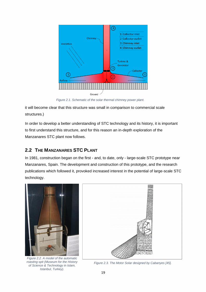
The solar thermal chimney (STC) power plant consists of three main components: the solar
collector, which is a large transparent canopy supported above the ground and open at the
periphery; a tall chimney, which is located at the centre of the collector; and a turbine and
generator set, which is located at the base of the chimney. Solar radiation heats the air
beneath the collector canopy via the greenhouse effect. The heated air becomes buoyant
and rises through the chimney. The buoyancy pressure difference generated draws air
through the collector and up the chimney, and the turbines at the base of the chimney
extract energy from the airflow. A typical configuration of the STC is shown in Figure 2.1.
2.1 STCS: HISTORY AND CONTEXT
The simple operating concept of the solar thermal chimney power plant has been outlined in
the preceding chapter. Their simplicity has appealed to engineers and inventors throughout
history. At a fundamental level, the STC is a device for extracting energy from a buoyant
updraft of heated air. This idea is not new. A design for an automated rotating chicken spit
powered by hot air rising from the fire is attributed to Leonardo da Vinci [6], though earlier
designs based on the same operating principle were produced by Islamic scholars (Figure
2.2). The concept of useful buoyant airflow has also been used for centuries as a passive
ventilation system in buildings.
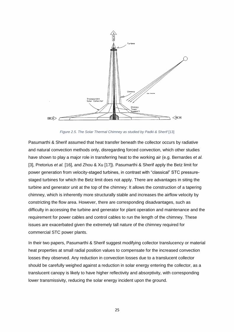
The first device which would be recognised as a modern STC was the Proyecto de motor
solar, or ``solar engine project'' proposed by Spanish artillery colonel Isidoro Cabanyes in
1903 [7]. Cabanyes' design consisted of a large brick structure with a chimney which
contained a form of wind propeller and to which was attached a glass solar air heater
structure (Figure 2.3). At the French Academy of Sciences in 1926, Dubos proposed that a
large-scale STC structure could be affixed to a suitable mountainside in order to avoid the
complex structural issues associated with constructing a tall, slim chimney [8].
In 1931, the same concept was featured in a futurist publication by Günther [7]. However,
serious scientific interest in STC technology developed only recently, following the
construction and operation of a large-scale research plant in Manzanares, Spain. (Although,
19
it will become clear that this structure was small in comparison to commercial scale
structures.)
In order to develop a better understanding of STC technology and its history, it is important
to first understand this structure, and for this reason an in-depth exploration of the
Manzanares STC plant now follows.
2.2 THE MANZANARES STC PLANT
In 1981, construction began on the first - and, to date, only - large-scale STC prototype near
Manzanares, Spain. The development and construction of this prototype, and the research
publications which followed it, provoked increased interest in the potential of large-scale STC
technology.
Figure 2.3. The Motor Solar designed by Cabanyes [45].
Figure 2.2. A model of the automatic roasting spit (Museum for the History
of Science & Technology in Islam, Istanbul, Turkey).
Figure 2.1. Schematic of the solar thermal chimney power plant.

20
Table 2.1. Key dimensions and materials used in the Manzanares STC [3].
Properties Values
Collector radius 122 m
Collector height 2 m
Chimney internal radius 5 m
Chimney height 194 m
Collector materials PVF & PVC film, 0.1mm thick, mounted on
steel frames.
Ground-based heat absorption
materials
Dark top-soil, light-coloured limestone, coal
spoil, bitumen.
Chimney materials Steel sheets, 1.2 mm thick, with guy cables.
Nominal output power 50 kW
This prototype, hereafter referred to as the Manzanares STC, was funded by the
government of West Germany and it was designed, constructed and operated by Schlaich,
Bergermann und Partner, a German civil engineering consultancy. The plant was
commissioned for operation on 7th June 1982. It was a research prototype and as such its
purpose was to facilitate research into the thermo-fluid operating principles of STCs, as well
as exploring STCs’ response to environmental factors, different system configurations and
different material properties. Despite being a reasonably large structure (its full dimensions
are given in Table 2.1), it was too small to produce power at an economically viable level.
The Manzanares STC was nonetheless a striking structure, as seen in Figure 2.4.
The chimney constructed for the Manzanares STC was 194 m tall and 10 m in internal
diameter. It was constructed from pre-fabricated steel sections 1.2 mm thick with additional
reinforcing rings for increased stiffness. It was guyed, with cables in three directions to
support the structure under lateral wind
loading. The steel chimney sections were
transported onto site individually, where
they would be affixed to the lower end of
the chimney sections already in place. The
chimney would then be jacked up to allow
further sections to be attached from
underneath, in a construction process
developed especially for this application by
Schlaich, Bergermann und Partner. Figure 2.4. An aerial photograph of the Manzanares research prototype STC [45].

21
The collector was constructed from a steel space frame (the canopy support structure), onto
which was laid PVC and PVF films (about 0.1 mm thick). These films were held in place by
weights on the top surface of the canopy, which prevented it billowing in high winds.
Different plastic films were used to assess the performance of the collector when different
materials were employed. The turbine was a single vertical-axis pressure-staged turbine in a
moulded housing to guide the airflow from horizontal radial flow as it exits the collector to
vertical axial flow as it enters the chimney. The turbine was rated at 50kW.
The Manzanares STC delivered at most approximately 40 kW of electricity [9]. It was highly
instrumented and Schlaich, Bergermann und Partner were capable of measuring a range of
properties, including thermal and optical material properties. In a paper by their engineers
[9], it is calculated that approximately 30 % of the heat from the sun is delivered directly to
the working air, whilst the remaining 70 % is either lost via convection and radiation to the
atmosphere or else conducted into the ground. Heat conducted to the ground is returned
later when the ground surface temperature falls and Haaf et al. [9] calculate that once this
effect is included, the collector efficiency reaches 50%. Their research indicated that whilst a
glass canopy would deliver a slight performance improvement over plastic film, the choice
should be made on the basis of the economics. The performance improvement is small, and
glass is more expensive but more durable and has a greater operational lifetime. Haaf et al.
estimate a lifetime of 20 years for glass and 7 years for plastic film [9].
Much attention was paid to the heat performance characteristics of the materials used in the
Manzanares STC. Haaf and his colleagues found that they over-estimated the absorptivity of
the ground (they initially predicted 0.80 ), due partly to the fact that construction
disturbed the high-absorptivity topsoil, exposing low-absorptivity limestone beneath
( 0.65 ). They also found that high ground absorptivity is fundamental to good plant
performance, and that the relationship between power output and ground absorptivity is
nearly linear. Experiments were carried out to improve ground absorptivity, including laying
coal spoil ( 0.85 ) and bitumen ( 0.91 ), leading to increased retention of heat by the
portion of the collector ground covered with high-absorptivity materials. The canopy's
thermal and optical properties were also examined. Unlike many solar thermal technologies,
the STC's collector is not an imaging collector. It does not require direct sunlight and can
continue to operate under diffuse radiation. This same property also makes it more resilient
to dust and dirt which builds up on the collector canopy. It was found that plastic films with a
lower surface roughness were better suited to self-cleaning in the occasional rainstorm. Rain
was capable of returning the solar transmission to within 2 % of its initial transmission value
at installation. After long periods without rain, manual cleaning improved transmission by up
to 12 %.

22
Haaf et al. created a mathematical model which was validated by their prototype STC plant
[6]. This model utilised the Boussinesq approximation, which assumes that density change is
a function of temperature only, and is valid for small density changes. The Boussinesq
approximation was created as a method of simplifying the simulation of natural convection
flows by permitting them to be calculated within a steady and incompressible flow regime. A
derivation and an explanation of its use in STC modelling is given in Chapter 3.
Haaf et al. [6] presented a simple model for calculating the working air temperature rise
across the collector, in which the collector efficiency is known to be a function of mass flow
rate and collector air temperature rise – that is, ( , )c c T m . The transformation from
incident solar energy to thermal energy contained within the working airflow does not happen
at constant efficiency along the collector radial length. Haaf et al. outline an energy balance
analysis for a discretised collector section which permits them to calculate energy flows
between the collector canopy, working air flow, and ground surface. More details on this
modelling strategy are given in Chapter 3. A simple fixed efficiency is assumed for the
turbine.
2.3 OVERVIEW OF STC LITERATURE
The Manzanares STC kick-started academic interest in STC technology, which has grown
into the large body of literature we encounter today. Academic literature is divided into
papers which demonstrate new modelling or prototyping techniques, with which better STC
models are built, and papers which use existing approaches to interrogate a particular
aspect of STC performance, e.g. in parametric studies or location-specific studies. The
models in existence today can be defined as either analytical models or computational fluid
dynamics (CFD) models, some of which utilise self-generated code and some of which use
commercial CFD packages.
The simplest models, presented in Section 2.4, assume efficiencies for some or all of the
STC’s main components, or else they make assumptions regarding heat transfer coefficients
in the collector, which more complex models have found to be dynamic along the collector
radial path. More comprehensive models, in Sections 2.5 & 2.6, simulate the airflow through
the collector to calculate the air condition at the collector outlet. Analytical models generally
assume the flow through the collector to be axisymmetric, reducing it to a one-dimensional
flow problem, if the velocity profile with height is assumed to be constant. Computational
fluid dynamics (CFD) studies have been undertaken, permitting researchers to study the
performance of a particular STC configuration in depth. In some cases, in the absence of
physical research plants, CFD studies have been used to lend confidence to analytical

23
models. Section 2.7 presents research plants of various scales - though none approached
the scale of Manzanares – which were most commonly used as validation tools.
Optimisation of STC dimensions is considered in Section 2.8. Optimisation studies typically
aim to minimise the levelised electricity cost, or cost per kilowatt-hour of electricity
generated. For this, cost models are required as presented in Section 2.9.
This literature review considers the current state-of-the-art for STC models of all forms,
exploring the relative advantages and disadvantages of each and assessing the validity of
any assumptions made. Through this process, topics which would benefit from further
research were found and the most appropriate form of STC model for our own development
can be identified.
2.4 SIMPLIFIED MATHEMATICAL MODELS
A simple mathematical model was drawn up by Zhou et al. [10], in order to simulate a STC
located in China. The model was steady state and the independent variables under scrutiny
were insolation, collector area and chimney height. The working air was assumed to be an
incompressible ideal gas and was treated as frictionless. The ground beneath the absorber
was assumed to be at the same temperature as the ambient air. In common with most
analytical STC models, the thermo-fluid properties of the collector are assumed to be
axisymmetric about the chimney, reducing the collector simulation to a one-dimensional
problem. Energy balance equations were derived for each component in the collector and
each component is treated as a homogeneous unit of one temperature, i.e. the temperature
does not vary with collector radial position. The air pressure through the collector is assumed
to be constant. It was assumed that the density of the air within the chimney does not
change with height, leading to an under-estimation of the chimney inlet velocity. The power
output is calculated assuming a velocity-staged wind turbine, as opposed to a pressure-
staged air turbine, meaning it extracts power from the dynamic pressure drop across the
turbine, as opposed to the static pressure drop. The model's outputs were validated against
a small-scale prototype constructed by the authors. The prototype was modular and the
chimney height could be varied from 1m to 8m, whilst the collector radius could be varied
from 1m to 5m. Based on local construction costs, a cost-optimised STC was specified. It is
interesting to note that, despite the many simplifying assumptions, the model was
successfully validated against the lab prototype. It can therefore be concluded that in
laboratory-scale STCs, air-surface friction is not an important factor in determining power
output and that the assumption of ground temperature equal to ambient temperature has a
similar insignificant influence on accuracy.

24
Hamdan [11] produced a simple analytical model of the STC. The model utilises
incompressible flow, assumes no pressure drop through the collector, no temperature or
density change through the chimney and a 100 % efficient turbine. It should be noted that
collector heat losses (via convection and radiation) are not considered. This assumption will
increase collector T significantly, which, due to the coupled nature of the collector and
chimney, also increases the system mass flow rate. Other authors have found the
thermodynamic efficiency of the collector (i.e. the efficiency with which the collector delivers
solar heat to the airflow) to be in the order of 50 % - 60 % [12]. Thus the assumption of zero
heat loss combined with the assumption of a zero-loss turbine leads to a model which
significantly over-estimates the system output power. Despite these assumptions being
weighted in favour of over-estimating the power output, Hamdan shows good correlation with
other authors' models. The over-estimation is countered by the assumption of constant
density throughout the chimney, which will lead to an under-estimation of chimney pressure
drop. The solar insolation (solar heat input flux) is also particularly low, set at various points
in the paper at 185 W/m2 and 263 W/m2.
A small group of authors have investigated a variation upon the ``classical'' STC design
whereby the turbine & generator were located at the chimney exit, at height. Padki & Sherif
[13] developed a set of differential governing equations to describe the performance of their
STC. They also proposed constructing the chimney with reducing cross-sectional flow area,
in order to increase flow velocity through the chimney and provide greater structural stability.
It should be noted that this design requires a velocity-staged turbine similar to standard wind
turbines, which extracts power from the dynamic pressure drop, but different from the
pressure-staged turbine used in the ``classical'' STC design, which extracts power from the
static pressure drop. Padki & Sherif's STC design can be seen in Figure 2.5. This design
was analysed by Pasumarthi and Sherif [14], who also constructed a small-scale prototype
and tested the performance improvements brought about by extending the collector base
and installing heat absorber material beneath the collector canopy [15].
Pasumarthi and Sherif created a steady state, axisymmetric model which assumes
frictionless flow, a constant ground surface temperature (equal to ambient air temperature)
beneath the absorber and mean values of component optical properties to estimate heat flux
incident upon the absorber.
25
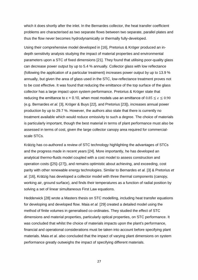
Figure 2.5. The Solar Thermal Chimney as studied by Padki & Sherif [13]
Pasumarthi & Sherif assumed that heat transfer beneath the collector occurs by radiative
and natural convection methods only, disregarding forced convection, which other studies
have shown to play a major role in transferring heat to the working air (e.g. Bernardes et al.
[3], Pretorius et al. [16], and Zhou & Xu [17]). Pasumarthi & Sherif apply the Betz limit for
power generation from velocity-staged turbines, in contrast with “classical” STC pressure-
staged turbines for which the Betz limit does not apply. There are advantages in siting the
turbine and generator unit at the top of the chimney: It allows the construction of a tapering
chimney, which is inherently more structurally stable and increases the airflow velocity by
constricting the flow area. However, there are corresponding disadvantages, such as
difficulty in accessing the turbine and generator for plant operation and maintenance and the
requirement for power cables and control cables to run the length of the chimney. These
issues are exacerbated given the extremely tall nature of the chimney required for
commercial STC power plants.
In their two papers, Pasumarthi & Sherif suggest modifying collector translucency or material
heat properties at small radial position values to compensate for the increased convection
losses they observed. Any reduction in convection losses due to a translucent collector
should be carefully weighed against a reduction in solar energy entering the collector, as a
translucent canopy is likely to have higher reflectivity and absorptivity, with corresponding
lower transmissivity, reducing the solar energy incident upon the ground.

26
2.5 COMPREHENSIVE MATHEMATICAL MODELS
There have been several papers published on the creation of in-depth analytical STC
models. They maintain the assumption of one-dimensional axisymmetric flow, but offer
various sets of assumptions about the STC flow and material characteristics.
2.5.1 Focus on Collector Simulation
Bernardes et al. describe a comprehensive analytical model with dynamic heat transfer
coefficients calculated along a discretised radial path within the collector [3]. Bernardes et al.
conceived the collector as a set of thermally-connected components, between which thermal
energy is conducted, convected or radiated at each discretised radial step. The set of
equations describing energy flow between components are solved via matrix inversion to
find the component temperatures. In this way, Bernardes et al. could simulate the impact of
changing material properties upon the performance of the STC.
Bernardes’ model was the culmination of a body of work including a study of natural
convection for radial laminar flow between two plates ([18], analogous to flow in the solar
collector), and his PhD thesis on STCs [19]. Three years later, in 2006, Pretorius and Kröger
[16] created a model of a large-scale STC plant, with environmental conditions from a
reference location in South Africa. Their model was particularly comprehensive, including
new equations for calculating heat transfer coefficients and a model for transient heat
storage, allowing the plant's potential for night-time operation to be evaluated. Friction
equations included in the model take into account the drag due to collector supports and the
chimney internal bracing spokes.
Both Bernardes and Pretorius utilise a radial discretisation technique in order to calculate
and account for component temperatures varying along the collector length. Bernardes,
Backström and Kröger came together to write a paper comparing the two models [20], and
specifically investigating the differences in heat transfer coefficients used by the two papers
and how they may have influenced the results. Both models calculate collector component
temperatures via energy balances, but only Bernardes explores the different collector
configurations with multiple transparent canopies to retain a greater proportion of the
incident solar energy. The greatest difference between the two models, beyond the friction
sources already identified, was the assumptions regarding flow development in the collector.
Pretorius' model [16] changes the collector canopy height with radial position, maintaining
the collector velocity approximately constant. The Bernardes model [3] assumes a level
collector canopy which does not change with radius. In developing the heat transfer
coefficient equations, Pretorius & Kröger characterised the airflow between the ground and
the canopy as a flow between parallel plates, and thus the flow can become fully-developed,
27
which it does shortly after the inlet. In the Bernardes collector, the heat transfer coefficient
problems are characterised as two separate flows between two separate, parallel plates and
thus the flow never becomes hydrodynamically or thermally fully-developed.
Using their comprehensive model developed in [16], Pretorius & Kröger produced an in-
depth sensitivity analysis studying the impact of material properties and environmental
parameters upon a STC of fixed dimensions [21]. They found that utilising poor-quality glass
can decrease power output by up to 5.4 % annually. Collector glass with low reflectance
(following the application of a particular treatment) increases power output by up to 13.9 %
annually, but given the area of glass used in the STC, low-reflectance treatment proves not
to be cost effective. It was found that reducing the emittance of the top surface of the glass
collector has a large impact upon system performance. Pretorius & Kröger state that
reducing the emittance to ε = 0.10, when most models use an emittance of 0.85 ≤ 𝜖 ≤ 0.90
(e.g. Bernardes et al. [3], Kröger & Buys [22], and Pretorius [23]), increases annual power
production by up to 29.7 %. However, the authors also state that there is currently no
treatment available which would reduce emissivity to such a degree. The choice of materials
is particularly important, though the best material in terms of plant performance must also be
assessed in terms of cost, given the large collector canopy area required for commercial-
scale STCs.
Krätzig has co-authored a review of STC technology highlighting the advantages of STCs
and the progress made in recent years [24]. More importantly, he has developed an
analytical thermo-fluids model coupled with a cost model to assess construction and
operation costs ([25]–[27]), and remains optimistic about achieving, and exceeding, cost
parity with other renewable energy technologies. Similar to Bernardes et al. [3] & Pretorius et
al. [16], Krätzig has developed a collector model with three thermal components (canopy,
working air, ground surface), and finds their temperatures as a function of radial position by
solving a set of linear simultaneous First Law equations.
Hedderwick [28] wrote a Masters thesis on STC modelling, including heat transfer equations
for developing and developed flow. Maia et al. [29] created a detailed model using the
method of finite volumes in generalised co-ordinates. They studied the effect of STC
dimensions and material properties, particularly optical properties, on STC performance. It
was concluded that whilst the choice of materials impacts upon the plant's performance,
financial and operational considerations must be taken into account before specifying plant
materials. Maia et al. also concluded that the impact of varying plant dimensions on system
performance greatly outweighs the impact of specifying different materials.

28
Gannon & von Backström [5] analysed the STC as a thermodynamic cycle. They plotted the
ideal (no-loss) cycle in order to calculate the limits of STC performance. They also simulate
thermodynamic performance with ``real'' (lossy) components, including a set of simultaneous
equations for solving the heat balance in the collector. They found that turbine efficiency is
not constant, and included calculations for turbine efficiency in their model, thus improving
accuracy. Petela [30] wrote a thermodynamic analysis of the STC in terms of the plant's
exergy, exergy being the maximum possible work a system can do which brings it into
equilibrium with a thermal reservoir.
More recent contributions by Bernardes [31], [32] have studied flow between nearly-parallel
walls, of the type seen in a STC collector with a sloping canopy. This work lays the
foundations for highly-developed bespoke heat transfer coefficient equations to be derived,
as it has led Bernardes to create equations for both the Nusselt Number and friction factor
for these particular scenarios. The bulk of the work presented by Bernardes thus far is
involved in identifying and defining the conditions under with mixed convection can exist,
and, by extension, identifying the flow structures which will form as a result.
Some authors have made use of mathematical models to assess their own innovations and
improvements to the classical STC collector design. Gitan et al. [33] constructed a
comprehensive mathematical model of the solar collector to assess the impact upon
performance of their “tracking solar collector” innovation. The tracking collector canopy
changes its slope angle according to the azimuthal angle of the sun, to reduce the cosine
losses caused by incident solar radiation striking the canopy at an angle other than the
normal. The model itself presents a detailed treatment of the solar radiation striking the
collector, including direct and diffuse insolation. The findings are validated with a small-scale
STC prototype, constructed at their university in Iran. The authors also simulated the STC
power plant across the year and found that when a fixed-angle canopy is specified, a
collector slope of 10° delivered the greatest power output.
2.5.2 Focus on Chimney Simulation
Tingzhen et al. [34] developed a comprehensive model and noticed a discrepancy between
their results and those produced by Pastohr et al. [35]. Pastohr et al. show the static air
pressure rising through the collector whereas the model created by Tingzhen et al. shows
the static pressure falling through the collector. Similarly, Sangi et al. [36] produced
comprehensive analytical and CFD numerical models, and reached a similar conclusion that
static pressure should fall as the air travels through the collector.
Tingzhen et al. identify the need to develop a comprehensive analysis of relative static
pressure through the chimney component. The pressure difference within the chimney is
29
generated by the buoyancy of the heated air entering at the base, and attenuated by wall
friction, friction due to spoke-wheel supports (if any) and viscous shear stress (generally
assumed to be small and therefore neglected). Tingzhen et al. (along with Zhou et al. [10])
state that the pressure drop due to buoyancy through the chimney is calculated by:
0
( )d ,chH
chp g z (2.1)
Where ch
H is the height of the chimney, from the ground to the outlet; is the
environmental air density at ground level; ch
is the working air density at the chimney inlet;
and dz is the infinitesimal change in chimney height. This is in agreement with the literature.
However, Tingzhen et al. and Zhou et al. both go on to assume that a and ch are
constant, which, they argue, is valid for small chimneys. Thus the integration is simple and
the pressure difference can be expressed as:
( )ch chp g H (2.2)
In making this assumption, the researcher under-estimates the pressure difference
generated by the chimney, particularly for very tall chimney structures. The benefits of
extending the height of the chimney come partly from the atmospheric density lapse rate and
to ignore the effect of the lapse rate understates the pressure difference across the chimney.
Tingzhen et al. suggest that once the chimney height under consideration exceeds 1000m, a
form of ``bulk air density'' may be used to capture the density variation with height, yet still
provide a pressure difference equation with the simplicity of Equation (2.2). There is a more
comprehensive solution in which the change of density with altitude is assumed to be an
isentropic process. This analysis finds that some method of accounting for density variation
with height is required for all heights of chimney. It should be noted that the model by Zhou
et al. [10] is described by the authors as a simple model and that the same authors
subsequently produced a more complex model in which the change of density with height
was modelled by an empirical lapse rate equation [37]. Tingzhen et al. define air properties
within the collector by means of an un-modified Bernoulli equation. The Bernoulli equation is
only suitable for flow in a stream-tube where neither momentum nor energy crosses the
stream-tube boundary. The airflow beneath the collector is receiving solar energy and thus
the Bernoulli Equation is not suitable. A more suitable equation, similar to the Bernoulli
Equation, would be the Steady-Flow Energy Equation.
Most available models treat the working air as a single-phase gas, that is either as dry air or
as air with fixed relative humidity. However, Ninic [38] wrote a paper assessing STC

30
performance for both dry and humid air, and for varying chimney heights. Ninic suggests that
vortices could be induced at the collector outlet, allowing the air to maintain vortex motion in
the column directly above the collector outlet turbine, and potentially obviating the need for a
tall chimney.
2.5.3 Focus on Turbine Simulation
Fluri & von Backström [39] wrote a paper exploring the impact of turbine layouts on plant
performance. Four different turbine configurations were considered, with the design options
being single-rotor or dual-rotor counter-rotating turbines, each with or without inlet guide
vanes. They concluded that a single rotor layout without inlet guide vanes performed poorly
because it induced swirl at the turbine exit, increasing kinetic energy loss, and that the
optimum efficiency of the remaining three layouts was reached only within a narrow
operating range. Fluri & von Backström also noted that the highest efficiencies were
achieved at low speeds, leading to undesirably high torque. For future work, they suggested
developing a cost model in order to establish which turbine layout would provide the lowest-
cost electricity. Borrowing design ideas from hydroelectric power stations, Gannon & von
Backström [40] proposed a STC with a single-rotor turbine mounted on a vertical axis with
inlet guide vanes to introduce pre-whirl in the airflow before it reached the turbine blades.
This is standard practice for hydroelectric turbines and it ensures that the turbine can extract
the maximum power from the flow and that the exit kinetic energy of the flow is minimised.
Gannon & von Backström propose re-designing the solar collector supports as inlet guide
vanes, thus minimising material consumption. A further paper by the same authors - von
Backström & Gannon [41] - investigates in detail the efficiency of a single-rotor axial turbine
with inlet guide vanes and flow diffuser. The authors note that most STC models to date
assume a fixed value for turbine efficiency and do not investigate the matter further. Their
analysis consists of mathematical modelling and experimental testing using a prototype
turbine model with a blade diameter of 720 mm. They found that total-to-total turbine
efficiencies of up to 90 % are achievable, but not necessarily over the full operating range.
Kirstein & von Backström [42] continued the analysis began in [40] and [41], modelling the
airflow through inlet guide vanes, through the transition from radial to axial flow and then
through the turbine and diffuser. As in the previous studies, the analytical conclusions were
supported by experimental results. In this paper, Kirstein & von Backström also included a
CFD analysis of a full-scale STC plant. Their analysis led to two empirical equations which
may be of use in STC optimisation studies.
There has been much debate regarding the optimum turbine pressure drop (generally
defined as a proportion of the total chimney pressure drop). Initial investigations set the ratio
of pressure drops at 2 / 3 [6], whilst later analyses suggested values in the range of 0.7 - 0.9

31
were optimal ([3],[16]). An investigation was carried out by von Backström & Fluri [42] in
order to establish analytically the optimum turbine pressure drop ratio. It was found that the
optimum pressure drop is not constant but in fact depends on the relationship between
available pressure drop and volume flow and on the relationship between system pressure
loss and volume flow. It was concluded that the STC could operate at maximum fluid power
(optimum turbine pressure ratio) with far lower volume flow rates and far higher pressure
drops than allowed under a constant-ratio assumption. Nizetic & Klarin [43] also studied the
issue of optimum turbine pressure drop ratio. Nizetic & Klarin considered the operation of the
STC as a thermodynamic cycle with losses. They calculated the optimum air velocity at the
chimney inlet, from which, if the chimney height is known, the optimum chimney pressure
drop can be calculated. They also calculated the optimum pressure drop across the turbine
as a function of air temperature increase through the collector. Once both these optimum
values are known, the optimum pressure drop ratio for maximum output power can be
calculated.
Validating comprehensive analytical STC models is difficult as complete validation would
require the construction of a large-scale STC plant. While some authors have built small-
scale research plants (see Section 2.7), many have also opted to develop CFD models to
provide a level of confidence in their analytical models.
2.6 CFD MODELS
Computational fluid dynamics (CFD) has been used widely to study the thermo-fluid
characteristics of STC power plants. Significantly more computationally intensive than
analytical models, CFD models have typically been used to study individual STC
configurations rather than exploring STC performance for a range of configurations. As such,
CFD models play two useful roles. Firstly, they can provide some confidence in validating
analytical models, which would be more capable of rapidly simulating a range of dimensions
and conditions. Secondly, CFD models enable researchers to study in great detail the
thermofluid mechanisms which give rise to certain aspects of STC plant performance. The
STC plants studied via CFD have tended to be on a smaller scale (i.e. the size of the
Manzanares plant) for the same reason. Additional simplifications - such as replacing the
heat radiation model with a constant-heat-flux ground surface - reduce computational
complexity further in some models.
2.6.1 Focus on Collector Simulation
Guoliang et al. [44] produced a numerical model of a STC, with dimensions similar to the
Manzanares prototype. They suggest that, under the right conditions, such a plant could
32
produce up to 120 kW (the Manzanares plant produced 40 kW peak [45]). They identify the
main system energy losses as being convection and radiation from the collector canopy and
heated air leaving the system at the chimney exit. Guoliang et al.'s numerical model was
two-dimensional and includes a pressure-staged turbine. Their analysis focussed on the
influence of turbine pressure drop and chimney pressure drop on other system parameters.
Pastohr et al. [35] produced a two-dimensional numerical model of the STC using FLUENT
CFD software. The dimensions used were those of the Manzanares prototype plant. Pastohr
et al. also develop a simple analytical model in order to corroborate the CFD findings and
compare the impact of additional work & computational resources (required for the CFD
model) upon output accuracy. The CFD model was axisymmetric and incompressible, with
the Boussinesq approximation modelling small density differences. Pastohr et al.
acknowledge that the STC requires a pressure-staged turbine, however including a
pressure-staged turbine requires iterative calculations in the CFD model. This is because the
pressure drop across the turbine affects the preceding pressure velocity (and, to a lesser
degree, temperature and density) of the air flowing through the collector. The altered
properties of the incoming air affect the turbine pressure drop (and the chimney pressure
drop), thus requiring a re-calculation. This process is repeated iteratively until the turbine
pressure drop converges and a stop condition is reached. Pastohr et al. utilise k
equations with grid adaption.
Sangi et al. [36] perceive the pressure equation for the STC as being key to correctly
determining how the system should be modelled. They develop the pressure equation
directly from the Navier-Stokes equations and carry out a CFD analysis in FLUENT to
confirm their calculations. The model is two-dimensional, axisymmetric and steady state.
The collector heat transfer equations take account of varying heat transfer coefficients and
temperatures along the collector radius and all heat transfer methods are considered
(radiative, forced convection, natural convection). The FLUENT simulation uses the k
turbulent energy model. Sangi et al., similarly to Tingzhen [34], noted the issue of rising
static pressure through the collector in Pastohr et al.'s model [35], and found that in their
model the static pressure dropped as the air flowed through the collector. Having placed an
emphasis on deriving the correct pressure equation for the STC, Sangi et al. proceed to
model the turbine as a velocity-staged turbine subject to the Betz limit, which states that the
maximum possible power that can be drawn from the airflow is 59.3% (16 / 27 ) of the kinetic
energy of the airflow. The turbines employed to extract power from the pressure difference of
the flow through the STC are, of course, pressure-staged turbines and as such they must be
modelled differently. Other than the disagreement over collector static pressure, Sangi et

33
al.'s results correlate well with the experimental results from the Manzanares prototype and
from Pastohr's model.
Bernardes [18], in developing his Masters thesis on the simulation of STC operation,
produced a study of natural convective heat transfer for laminar radial flows between two
heated plates, to approximate the STC collector. Subsequent studies have shown that the
flow within the collector is turbulent and fully-developed for most STC configurations within a
short distance of the collector inlet [46]. CFD studies of a similar topic have been undertaken
by Beyers [47] and Beyers et al. [48], who developed a three-dimensional thermo-flow CFD
model for radially-accelerating flow between rough parallel plates.
Koonsrisuk & Chitsomboon attempted to achieve dynamic similarity for a scaled model STC
by developing a single dimensionless variable [49]. Earlier efforts by the same authors saw
them define the flow in an STC by several dimensionless variables [50] and achieve partial
geometric similarity [49]. Both papers developed their ideas through dimensional analysis
and the Buckingham Pi Theorem. In their later paper [51], Koonsrisuk & Chitsomboon
assessed the performance of their fully geometrically similar models (from [51]) against their
partially geometrically similar models (from [49]) and geometrically dissimilar models. The
models are executed via CFD, under the assumptions of steady, laminar and inviscid flow.
The assumption of laminar flow is likely to be a limiting factor in the accuracy of the model -
most models, including the highly-developed analytical models by Bernardes [3], Pretorius &
Kröger [16] and Zhou et al. [37], show the airflow within the collector to be transitional or
turbulent.
While analytical models tend to assume the collector airflow as axisymmetric and radial, in
order to reduce the flow to a one-dimensional problem, CFD permits the researcher to
consider two- or three-dimensional non-radial flows with relative ease. Shriven et al. [52]
constructed a 2-dimensional CFD model of a STC of the same dimensions as Manzanares,
with which they undertook a sensitivity analysis to determine the plant’s performance as
some geometric parameters are altered. To limit computational complexity, the authors
assumed a constant ground heat flux of 800 Wm-2, and no turbine is included in the CFD
calculations. The presence of a turbine is modelled in the final calculations of power output,
but the effect of the turbine on the flow through the STC is not included in the simulations.
Sensitivity analysis requires multiple repeated simulations to determine the optimal STC
geometry within the given parameter space. As such this method would be prohibitively
expensive, computationally speaking, for much larger commercial-scale STCs. The authors
claim that best performance is achieved with a flat collector canopy (canopy slope 0 ),
contradicting the best-performing sloped and exponential canopies specified by Gitan et al.
34
[33] and Cottam et al. [53]. This may be due to the small size of the STC, but it is most likely
due to the assumption of constant heat flux from the ground surface. This assumption is not
held to be true in other works which have focussed efforts on thermodynamic rather than
fluid dynamic performance (e.g. Cottam et al. [53] and Hedderwick [28]).
Noting that thermodynamic aspects of CFD simulations of STCs are often simplified to
reduce computational expense, Huang et al. [54] presented a steady-state two-dimensional
CFD model of the Manzanares STC with an improved collector radiation model. Whereas
most models assume that air has a radiative transmissivity of 1 (and an absorptivity of 0),
Huang et al. have moved the model closer to reality by noting the spectral absorption of the
air and simulating its contribution to transferring heat to the working air. Furthermore, they
include the repeated reflection of radiative energy between the ground surface and the
canopy underside surface. As energy is lost radiatively through the canopy on each
reflection cycle, the authors claim that prior failures to include this mechanism have led to
over-estimates of collector performance.
Convection by ambient wind represents another major source of losses in the STC system.
Researchers have begun to use CFD to study the impact of ambient wind on STC
performance. An ambient crosswind will result in convective heat loss from the top canopy
surface and changes in wind direction within the collector, carrying away heated air from
beneath the canopy and thus harming collector performance. Ming et al. [55] developed a
CFD model of an STC with Manzanares dimensions, using the standard k turbulence
model and subjected it to a log-law ambient wind profile. It was found that performance was
not only affected by increased convected heat loss from the top canopy surface, and by
ambient wind velocity within the collector, but also by ambient wind airflow across the
chimney outlet, deflecting the chimney’s outlet air velocity and thus reducing the available
flow area. Furthermore, ambient wind can exacerbate issues with choking flows by providing
a downward component of the wind velocity at the chimney outlet. This effect would be
especially problematic during STC system start-up – when the cold dense air needs to be
cleared from the chimney – or during periods of low insolation when the upward chimney air
velocity may be weak. Conversely, the authors also found that the low pressures at the
chimney outlet caused by the ambient wind velocity generated a Venturi effect on the
chimney airflow, increasing chimney air velocity. Zhou et al. [56] simulated a STC with
ambient wind velocity at the chimney outlet only (not at the collector canopy). The authors
treated the air inside the chimney as a one-dimensional compressible flow. They found that
ambient wind velocity increases pressure potential through the chimney, and that this effect
increases with chimney height and decreases with increasing temperature difference, which
is influenced by collector area.
35
Having identified potential adverse impacts of ambient cross-wind, Ming et al. [57] attempt to
mitigate some of its negative effects with a wall (or other blockage) built around the collector
perimeter, a few metres away from the collector inlet. This wall reduces the impact of
ambient wind flow beneath the collector canopy, where it would otherwise create distortions
in the collector temperature field. Utilising the same CFD model and the same process as
Ming et al. [55], the authors found that the proposed wall abated the impact of the ambient
wind beneath the canopy significantly. With a free-stream wind velocity of 5 m/s and
optimum turbine pressure drop, the authors predict a five-fold increase in power output
compared to an identical system with no perimeter wall.
Shen et al. [58] use CFD and the k turbulence model to simulate a large-scale 10MW
STC power plant and assess the impact of ambient cross-wind. Rather than subject the STC
model to a log-law wind profile, the authors have tested the thermodynamic effect of ambient
wind at two key locations: At ground level (the collector) and at the chimney outlet. As
described above, the effect of ambient wind at ground level is to convect away heated air
from within the collector and additionally, the authors note, to cool the heated collector
surfaces, further reducing performance. The effect of the ambient wind at the chimney outlet
is positive, as the wind entrains the working air and increases the pressure differential
through the chimney.
A solution to the problem of ambient wind convective losses in the collector is proposed by
Ming et al. [59]. They propose sets of radial walls at the collector periphery to prevent
ambient wind in a non-radial direction, and compare this proposal to the use of low collector
inlets and sloping canopies to achieve the same objective. The authors found that both radial
partition walls and low collector inlets are effective in reducing losses due to ambient wind,
but that driving pressure differential is higher when radial walls are used than when low
collector inlets are specified.
2.6.2 Focus on Chimney Simulation
The buoyancy of the working air in the chimney, as the driving force for the STC system is
an important factor to which close attention should be paid when modelling the STC. Von
Backström & Gannon [60] developed a compressible flow model based on Mach Number
analysis for the chimney. Compressible flow modelling becomes more desirable with
particularly tall chimneys and von Backström & Gannon have studied chimneys up to 1500m
tall. Von Backström & Gannon have built a 1-D Runge-Kutta discretised grid upon which the
solution is calculated. Their sensitivity analysis established that their model produced
reasonable results even with only a single discretised step the height of the chimney. They
found that the pressure losses associated with the vertical acceleration of the flow within the

36
chimney are roughly three times those associated with surface friction. As such, they
recommend changes to the chimney design, particularly by flaring the internal flow area,
which will mitigate these losses. The same Mach Number approach is also detailed in a
technical note by von Backström [61]. Lebbi et al. [62] undertook CFD models for STCs with
a range of chimney dimensions, concluding that the greatest boost to power output is
available by increasing the chimney internal flow radius.
2.6.3 Focus on Turbine Simulation
Chergui et al. [63] analysed the STC concept through the use of FLUENT CFD software.
The analysis is limited to laminar flow with natural convection heat transfer only. These
approximations impose inaccuracies upon the model, as it has been shown that the flow in
most solar chimney collectors will be transitional and turbulent, and that heat transfer
methods in the collector will be combined natural and forced convection (e.g. Bernardes et
al. [3] and Pretorius et al. [16]). Tingzhen et al. [64] developed a numerical model of the
STC, with modelling effort focussed on the turbine. Simulations are undertaken using a
three-blade and five-blade turbine, for the dimensions of the Manzanares plant and for larger
MW-graded systems (𝐻𝑐ℎ = 400𝑚, 𝑅𝑐 = 1500𝑚). The model utilises k equations to
simulate turbulent flows and is constructed in FLUENT. The authors find that mass flow rate
falls and turbine pressure drop rises as the turbine’s rotational speed is increased. As power
generated is the product of pressure drop and volume flow rate, the authors identify optimum
turbine rotational speeds for both the smaller and larger STC configurations under study.
Kasaeian et al. [65] recognised the lack of three-dimensional studies of STC operation and
undertook an analysis of the STC turbine to assess the impact of using different quantities of
blades and different chimney geometries. The authors found that increasing the blade
quantity decreases the mass flow rate of air but increases the power output.
2.7 PHYSICAL EXPERIMENTS
While both analytical and CFD models can provide corroborative evidence of modelling
accuracy for one another, the only way to be certain of the performance of a STC is to build
an experimental rig and study it experimentally. Many researchers have combined CFD or
analytical models with experimental work, some re-configurable to test the effect of
dimensional changes. These physical experiments can validate the models and enable
researchers to predict more confidently the behaviour of large-scale STCs.
Kasaeian et al. [66] report on a 10m-tall STC research plant they have constructed. They
investigate the phenomenon of temperature inversion, whereby immediately after sunrise the
collector roof retains the cool air beneath it, even as the ambient air is warming in the sun.

37
This cooler air is not cleared from the system until the sun has heated it sufficiently, beyond
the temperature of the ambient air. This phenomenon delays the start-up of the STC on both
hot and cold mornings. They also explored the impact of collector inlet height upon collector
temperature rise, and concluded that smaller openings increase collector temperature rise
because they reduce the collector's exposure to convection losses from external winds.
Wei & Wu [67] describe the construction and testing of a novel STC built in the deserts of
Inner Mongolia, near Wuhai, China. This research plant had the advantage of being of a
relatively large size compared to other laboratory-based plants, although it remains far
smaller than commercial-scale STCs. The chimney stands 53 m tall, and its collector has a
surface area of 6300 m2. (Plans for a taller 200 m chimney had to be abandoned due to a
nearby airport.) However, it differs from other proposed STC designs in that the collector is
sealed with a wall around its perimeter, except on the side of the prevailing wind, where
there can be found a set of doors which rotate on a central hinge, permitting the doors to
guide the airflow into the collector. Thus this particular design generates power from high
(natural) wind velocity through the turbines, as well as thermally-generated buoyant airflow.
However, the presence of the walls around the majority of the collector’s perimeter impose a
pressure drop on the airflow, leading to a corresponding loss of power.
Wei & Wu assume isobaric airflow and create a simple thermodynamic model for the
buoyant updraft component of their plant’s operation, in which air properties are calculated at
the collector outlet, the chimney inlet and the chimney outlet. Additionally, Wei & Wu include
power generated by natural wind velocity, enabling the plant to generate power in the
absence of direct sunlight. The operating data provided shows a peak power output of
approximately 30 kW, achieved at low insolation but with high wind velocity.
Physical research plants have been constructed by other researchers to validate the
analytical models they have developed. Pasumarthi & Sherif [15] built a research plant to
validate their analytical model. It had a chimney 8 m tall and a collector diameter of 9 m.
Heat convection from the ground to the working air was aided by an aluminium plate and
black visqueen absorber material laid on the ground beneath the collector, with heat losses
to ground minimised by a layer of polystyrene foam beneath. They were able to undertake
some parametric studies by extending the collector to 18.2 m in diameter. Their physical
research plant validated their mathematical model, which was also validated against
performance data from the Manzanares STC, delivering a power output accurate to within
9.5 % of the recorded data. Kalash et al. [68] constructed a research plant with a sloped
collector (and without a turbine), and recorded 40 days of continuous performance data, with
a matrix of temperature sensors in the collector and air velocity sensors at the chimney inlet.

38
On the ground beneath the collector they laid a thermal absorption layer made from
compacted earth. The compacted earth had a low thermal inertia (low specific heat capacity)
and it returned absorbed heat rapidly to the working air. The authors concluded that it was
therefore unsuitable for enabling continued power generation during overcast periods or into
the night. Further details on sloped-collector STCs are found in Section 2.11. Zhou et al. [69]
studied the effect of temperature inversion (cold air in the chimney) on STC start-up shortly
after sunrise, using a research plant with a collector 10m in diameter and a chimney 8m tall.
A sufficient temperature increase within the collector is required to counter the dense cool air
within the chimney and begin the airflow through the STC, delaying the time at which STC
generation starts after sunrise.
A striking departure from conventional STC canopy designs was presented by Eryener et al.
[70], in which they introduced the “transpired solar collector” (TSC). Unlike a normal
collector, the TSC is sealed at the periphery with a vertical wall and the canopy consists of
metal material containing a plethora of small holes, as shown in Figure 2.6. The buoyancy
pressure difference draws air through the holes in the canopy, and in the process heat is
transferred to the air at greater efficiency than would be the case for the conventional
collector. The authors also claim reduced heat loss into the ground, as the ground material
does not first need to be heated in order to then heat the air. Improved canopy efficiency can
reduce collector size, reducing cost and bringing the STC closer to economic viability.
Eryener et al. have tested the feasibility of this design innovation with a prototype in Turkey.
The prototype is reasonably large, with a chimney height of 16.5 m and a collector surface
area of 110 m2. While the authors have deployed their TSC innovation for the majority of the
canopy area, they have used an amount of transparent polycarbonate to facilitate plant
growth within the collector. The polycarbonate material permits light to enter the collector,
signifying that some heat will be convected from the ground to the working air, after the
Figure 2.6. Transpired solar collector compared to "conventional" STC collector. Note that the periphery of the transpired collector is enclosed [70].
39
ground has been heated by the incident solar radiation. Furthermore, sealing the periphery
with a vertical wall has the advantage of eliminating convected losses due to ambient wind,
but will impose a significant pressure loss upon the system.
Maia et al. [29] validated their CFD model with a research plant (Hch = 12.3 m; Rch = 1.0 m;
Rc = 12.5 m), achieving good agreement between their respective results, with the model
delivering data to within 2 % of the data recorded by the prototype. The authors undertook
parametric simulations with their validated CFD model to study the effect of changing
collector radius, chimney height and chimney radius. They observed air temperature ceasing
to increase beyond a limiting value through the collector, depending on the collector size.
Larger collectors deliver a greater total temperature rise, and generate this temperature rise
most rapidly at the periphery. This behaviour would benefit from further exploration, as it
suggests that the largest collectors in the study (Rc = 12.5 m; Rc = 20.0 m) are over-sized
for the given chimney dimensions, delivering no additional thermodynamic benefit.
Gholamalizadeh & Mansouri [71] constructed a large prototype STC in Kerman, Iran. It
consisted of a chimney 60 m tall, and 3 m in diameter, with a collector radius of 20 m and a
turbine for the generation of electrical power. In operating the prototype, the authors found
that the motive force generated was insufficient to rotate the turbine except at very high
levels of insolation ( -2800WmI ). As such, they identified a need to optimise the dimensions
of the STC’s components relative to one another to ensure power generation across a wide
range of ambient conditions, and they present a simple cost model with which they
undertake parametric studies to identify the STC configuration with the lowest specific cost.
A later paper by Gholamalizadeh & Kim [72] re-visited the issue of optimising STC
dimensions given a set of costs and ambient conditions. They developed an algorithm for
determining optimal STC dimensions using genetic optimisation, with the variables being
collector radius, chimney height, and chimney radius. Through the use of physical
experiments, several researchers (including Maia et al. [29]; Gholamalizadeh & Mansouri
[71]) have identified that certain design configurations are sub-optimal and hence there is a
need to optimise the STC design.
2.8 OPTIMISATION
Simply expressed, larger STCs generate more power. As such, an optimal design cannot be
specified without additional constraints, normally cost-based. Dehghani et al. [73] noted that
there exists a range of plant dimensions which could be considered physically optimal, with
different configurations delivering an equal (high) power output, and that as such a cost
metric is required to constrain the optimisation. They devised a multi-objective optimisation
40
routine with objective functions to minimise construction cost and maximise power output.
Their economic model is simplified for the purposes of optimisation (they note that it is not
intended to assess accurately the costs of building the STC), and is based on volume of
material used to construct the chimney, area of ground covered by the collector, and amount
of power generated (to determine turbine and powerblock costs). They demonstrate financial
penalties (in terms of levelised electricity cost) to over-sizing certain components, especially
the collector. Pretorius & Kröger [74] performed a similar thermo-economic optimisation and
identified large increases to power output which can be gained by constructing a wider
chimney, with relatively little additional capital. However, they noted that this increases the
likelihood of cold air inflow at the chimney outlet, and for this reason they assessed the
impact of cold air inflow on their different optimal STC configurations, noting that chimneys
wider than 400m in diameter were likely to encounter it. Gholamalizadeh & Kim [72] drew on
their experience with their physical STC prototype in Kerman, Iran, to define a genetic-
algorithm optimisation for the STC plant, in terms of thermodynamic efficiency, total cost,
and specific cost (£/kW peak). Ahmed & Patel [75] used a CFD STC model in an
optimisation scheme to determine the optimal dimensions for a STC with a chimney height of
10 m. The authors then constructed an experimental model at 1:2.5 scale to validate their
model. A STC of suitable dimensions for use in the Pacific Island nations was also
simulated.
Optimisation of STC designs requires a reliable cost model, but the problem of predicting
STC construction and operating costs is significant, with many variables to be defined.
Hence, researchers have created cost models with varying degrees of complexity to address
precisely this problem.
2.9 STC COST MODELLING
As with all large infrastructure projects, the cost of a commercial-scale STC power plant is
difficult to determine. Labour, materials and financing are all sensitive to the specific location
and context, as well as to the plant design. Various cost models have nonetheless been
produced, yielding a wide range of predicted costs. The cost of power generation is
expressed as levelised electricity cost, or LEC, which is simply the predicted total cost over
the lifetime of the plant divided by the predicted total energy generation over the lifetime of
the plant. As such, it has units of pounds sterling (or other currency) per kilowatt-hour.
A cost model for commercial-scale plants accompanied the Manzanares STC research [6],
whereby The authors predict the whole-life cost of a commercial-scale STC based on the
costs they incurred developing the Manzanares research prototype STC. The authors
calculated a levelised electricity cost (LEC) of 0.29 DM/kWh, or £0.25/kWh (inflation-

41
adjusted to 2016), for a 35 MW STC plant, or 0.25 DM/kWh (£0.22/kWh adjusted to 2016)
for a 180 MW STC, both located at a latitude of 28°N and with a plant amortization period of
20 years. Significantly lower costs are predicted by Schlaich et al. [12], ranging between
£0.05/kWh and £0.10/kWh for a 200 MW STC with a range of depreciation periods and
interest rates. Bernardes [19] and Schlaich et al. [76] also predicted commercially-
competitive LECs for STC power plants of sufficient scale, under the right financial
conditions (£0.03/kWh - £0.10/kWh). The high dependency of costs upon financial factors,
such as interest rates on finance and the rate of inflation, was corroborated by MSc research
projects investigating STC financial viability co-supervised as part of this thesis.
Fluri et al. [4] created a comprehensive financial model, with STC performance data
provided by the comprehensive thermo-fluid model created by Pretorius et al. [16], to resolve
the differences in predicted cost and provide a more detailed examination of the commercial
viability of STC power plants. Fluri et al.’s cost model differed from existing efforts in its
prediction of turbine costs in particular, which was based on a comprehensive model and not
upon an assumed cost per kW of peak power output. Similarly, the collector and chimney
material costs are based on component costs (e.g. glass, columns, and glass support
components for the collector), rather than a fixed cost per square metre. Fluri et al. found
levelised electricity costs to be 270 % - 340 % of those presented in earlier studies. These
findings cast doubt on the economic viability of STCs under the current state of the art.
However, Zhou & Xu [17] offer a reprieve for the commercial vision of STC power plants by
noting that the industry-standard depreciation periods of 20 years – 50 years need not apply
to STCs. As relatively simple structures with few moving parts, STCs can be expected to
have a longer operating lifetime perhaps beyond 100 years, reducing the predicted LEC
commensurably. Krätzig [26] expects an operating lifetime of 120 years for a large-scale
plant generating 320 GWh per year. He splits the financial forecast into two phases, with
capital costs met by an LEC of £0.08/kWh during an initial 30-year amortization period, and
an LEC of £0.01/kWh for the remaining 70 years to meet operation and maintenance costs,
including turbine repair and renewal. Several other authors have taken the same approach,
yielding low-cost energy generation once the initial amortization period has passed (Zhou et
al. [77] & Li et al. [78]).
In summary, the financial viability of STCs is uncertain, due to uncertainties inherent in large
construction projects and differences in projected performance of the STC plant. Long
operating lifetimes provide a powerful advantage for commercial STC proposals, but
extremely high capital costs are proving to be an obstacle.

42
2.10 STC HEAT & POWER MANAGEMENT
Some researchers have acknowledged that a degree of control over power output would
mean better financial performance, as electrical power could then be dispatched when it is
required, or when it can be sold for the best price. Furthermore, sufficient energy storage
would make the STC a baseload generator, eliminating the intermittency problems that
plague most renewable energy technologies. Thus researchers have a motive to develop
methods of control within the STC to direct heat into storage for later use or to the chimney
for immediate power generation.
Bernardes & von Backström [20] identify that some output power control is achieved by
controlling the pressure drop across the turbine or by controlling the volume flow rate. It was
found that the pressure drop ratio (turbine pressure drop to total chimney pressure drop) was
not constant throughout the day, and depended on the heat transfer to the air in the
collector. Thus the model was particularly susceptible to differences in the heat transfer
coefficient schemes employed. Bernardes & von Backström were able to identify these
differences as they had the use of models by Bernardes et al. [3] and Pretorius & Kröger
[16]. Bernardes & von Backström [79] studied the performance of an STC with turbine
pressure ratio or the volume flow rate as independent variables. It was found that, in line with
the majority of the more recent literature, the optimum pressure drop ratio was in the range
0.8 90 .x , depending on the scheme employed to determine heat transfer coefficients
(either that of Bernardes [3], or of Pretorius [16]).
Rudimentary power control can be achieved by the addition of a second transparent canopy
below the first canopy (Zhou et al. [45]). Actuated grilles located between the lower canopy
and the ground control the pressure drop across the lower collector section. The lower
canopy helps retain a greater quantity of the radiated solar heat by increasing the
greenhouse effect. By varying the mass flow rate through the grilles, the rate of heat transfer
between heated ground and air can be controlled.
The ability to control STC power output relies upon the ground, or heat-storage materials laid
upon the ground, to act as a thermal capacitor and return additional heat to the air when
solar input falls away. With this in mind, it is important that the mechanisms of heat transfer
into and out of the ground or heat storage medium are well understood. Many of the
comprehensive STC models include heat storage media within the collector (Bernardes et al.
[3], Pretorius et al. [16], Ming et al. [80]), normally sealed bags of water (chosen for its high
specific heat), or cheap construction materials such as gravel or bitumen.
Bernardes & Zhou [81] analysed the impact of sealed water bags deployed as heat storage
materials beneath the collector canopy. It was found that in order for them to retain a

43
sufficient quantity of heat to
permit night-time power
generation, they needed water
bags 1m tall, representing an
unfeasible amount of water,
given the large collector area of
commercial-scale STCs
(EnviroMission's collector for a
200MW STC will have an area
of 41.27 km2). It was found that
a heat insulator layer beneath
the water bags was also essential, as the contact with the water bags increased the
temperature at the water bag / ground surface boundary and led to increased heat losses
into the ground. A shallow water bag layer (thickness = 0.20 m) leads to a significantly
higher ground surface temperature ( 57max
T C ) compared to that with no water bags
deployed ( 43max
T C ). As the water bag thickness is increased, the maximum ground
surface temperature decreases again due to thermal stratification of the water. The high
specific heat of water, a desirable quality for thermal heat storage, also leads to an increase
of heat loss into the ground as the temperature difference between the ground surface and
the water bags (upon which heat transfer depends) remains high despite the heat loss from
the water bag to the ground.
Utilising the same model, Bernardes [82] examined the influence of soil and ground material
properties on ground heat storage performance. He concludes that the issue is complex and
that further investigation is needed to develop confidence in the simulated results. Soil heat
transfer is complex due to the material’s inhomogeneity and the presence of moisture.
Hurtado et al. [83] studied the issue and concluded that for a STC to operate as a base-load
generator, the soil on which it is constructed needs to be of low thermal diffusivity and high
thermal inertia, with compacted soil increasing the power generated.
2.11 SLOPED-COLLECTOR STCS
Given the widely-acknowledged difficulties associated with building a tall chimney structure
of the scale required by a commercial STC, and the uncertainty surrounding STC costs,
some researchers have sought methods to achieve the required height difference without
exposure to the same level of technical and financial risk that a tall slender chimney brings.
One popular solution is the concept of the sloped STC power plant, in which the collector is
Figure 2.7. Sloped STC concept [88].

44
installed on the slope of a hill or mountainside, with a shorter chimney at its peak (Figure
2.7). The collector of a sloped STC does not normally extend fully 360° around the chimney,
with the exact collector size instead determined by the geography of the site. Combined flat
and sloped collectors are also envisaged, whereby the collector extends beyond the
selected slope over further flat land.
Modern research efforts on sloped STCs only appeared in 2005, when Bilgen & Rheault [84]
proposed a 5 MW sloped STC and identified three suitable locations in Canada. They note
the lack of heat transfer coefficient equations suitable for flow between two parallel inclined
plates, and in their place the authors identify empirical relations for Nusselt Number and
Rayleigh Number in open-channel inclined flows ([85], [86]), which are then adapted for flow
between parallel inclined plates. Bilgen & Rheault note that the sloped STC permits a
reduction in chimney height by up to 90 %, while generating up to 85 %, from its Canadian
location, of the power output delivered by a flat STC of comparable size in a high—insolation
(desert) location.
The difference in performance between a flat and a sloped STC is studied by Cao et al. [87].
The authors discovered that an increased collector slope angle delivers a higher
performance during the winter and a lower performance during the summer. They found that
the optimum slope for maximum annual energy generated was approximately 60°. Their
model, presented in detail in Cao et al. [88] describes the solar energy input to the sloped
STC system as being dependent upon the collector slope angle, as well as the quantity of
direct and diffuse solar energy available. They utilise a system of collector thermal
components with energy balances governing their temperatures, as described by Bernardes
[3], but with modified heat transfer coefficients to include the collector slope. The collector’s
momentum equation is not defined, but the air is assumed to be incompressible Boussinesq,
with no fluid internal shear stress or surface shear stress.
A comprehensive model of the sloped collector, with all governing equations defined, is
provided by Koonsrisuk [89]. The momentum and energy equations both include height
potential terms, which are normally neglected in flat-collector STCs. Koonsrisuk validates his
analytical sloped STC model with a CFD model, showing good agreement for all plant
parameters. Koonsrisuk goes on to develop his model using Second Law analysis [90],
whereby the plant efficiency is determined by the system’s power output relative to its
reversible power output (as defined in [91]). However, Koonsrisuk assumes that the collector
efficiency is fixed at 0.56c , when other studies have shown it to depend on insolation
and the velocity of the working air through the collector [3]. Zhou et al. [92] develops the
study of the sloped STC with a steady compressible-flow model. Including air humidity in

45
their model, the authors note that the increase in temperature due to the latent heat of
evaporation is enough to preclude further evaporation.
Kalash et al. [68] present the only experimental work on sloped STCs to date. They
presented a small-scale sloped collector structure (area of 12.5 m2), with a short chimney (9
m tall), and they observed the collector’s absorption layer (made of soil and gravel)
increasing in temperature throughout the morning. Further studies using this experimental
apparatus were made impossible by Syria’s ensuing civil war, but Kalash et al. did produce a
review of sloped STC technology developments to date [93], concluding that further
research, especially numerical and CFD studies, would help to increase understanding of
this technology.
2.12 COLLECTOR CANOPY PROFILES
The role of collector canopy shape in improving power plant efficiency and thereby reducing
STC levelised electricity cost has received limited attention. Researchers have long
recognised that different canopy profiles (changing canopy height along the radial length)
have an impact on the condition of the air within the collector and thus impact the power
output. The main profiles used in the literature are: flat; constant-gradient sloped; and
exponential, in which the canopy height rises exponentially from collector inlet to the central
collector outlet.
Across eighteen papers presenting STC models surveyed in preparation for this thesis, nine
utilised flat canopy profiles (Bernardes et al. [3]; Cottam et al. [94]; Fasel et al. [95];
Gholamalizadeh and Mansouri [71]; Guo et al. [96]; Haaf et al. [6]; Koonsrisuk [89]; Ming et
al. [55]; Sangi et al. [36]); six utilised a constant-gradient canopy (von Backström [97];
Dehghani and Mohammadi [73]; Gannon and von Backström [5]; Kasaeian et al. [66];
Pasumarthi and Sherif [14]; Zhou et al. [10]); and three utilised an exponential canopy profile
(Fluri et al. [4]; Pretorius and Kröger [16], [74]). Bernardes [7] investigated the effect of
different canopy profiles on the air velocity and heat transfer in the collector. Pretorius and
Kröger [16], [21] undertook brief studies of the role of the exponential canopy profile shape in
determining power output, concluding that an exponential canopy designed such that it
created a collector with constant cross-sectional flow area produced the greatest power
output. Pasumarthi and Sherif [14] studied the performance of a small-scale physical
prototype STC with three different configurations of the collector, varying collector size and
materials used. They concluded that introducing an intermediate absorber in the collector
has the potential to boost mass flow rate.
46
Koonsrisuk and Chitsomboon [98] studied the impact of canopy and chimney profile
parameters by investigating flow area changes within the STC, with a view to increasing
power output. They derived a theoretical expression showing how a collector canopy rising
towards the chimney and a flaring chimney can boost power output by up to 400%,
validating their theoretical calculations with CFD analysis. Additionally, Hu & Leung [99] used
a simple mathematical model to establish that divergent chimneys can increase power
output by many times, but further that the optimal ratio of inlet area to outlet area depends
on the height of the chimney. Koonsrisuk & Chitsomboon’s model of the STC was limited to
a constant heat transfer flux to the air over the collector area, and the turbine was not
modelled. However, they provide compelling evidence that canopy designs other than the
flat profile can lead to significant power gains. Beyond this, the impact of changing canopy
profile types or parameters has not been studied in detail. Furthermore, extreme canopy
heights, complex curvatures, and precise engineering tolerances are likely to increase
canopy construction costs. There is considerable scope to develop a canopy which is both
easy to construct and retains the performance advantages acquired through the use of non-
flat canopies, and this is considered in Cottam et al. [53], presented as part of this thesis in
Chapter 5.
2.13 STC SYSTEM SIZING
There are several studies which have examined the impact upon STC performance of
varying STC dimensional parameters or deploying the STC models within an optimisation
scheme. They include Pretorius & Kröger [21]; Maia et al. [29]; Cottam et al. [94], [100];
Gholamalizadeh & Mansouri [71]; Gholamalizadeh & Kim [72]; and Dehghani & Mohammadi
[73]. These authors have all articulated the need for judicious selection of STC dimensions,
but the thermo-fluid processes which govern the relationships between relative component
dimensions and STC performance remain unexplored. These mismatched dimensions
represent wasted expenditure, which must be avoided if commercial viability is to be
achieved. Understanding the thermo-fluid processes which govern these matched
dimensions will enable researchers to determine, with confidence, the appropriate STC plant
dimensions for their locations, power demand and budget.
Analysis of STC performance across a range of component dimensions requires an
analytical model capable of simulating multiple STC configurations rapidly. Parametric
studies such as these are typically undertaken using computational models. Comprehensive
models incorporating surface friction; ground heat loss; ambient, convective and radiative
losses; and ambient pressure lapse rates have been presented by Bernardes et al. [5], and
by Pretorius & Kröger [6]. Such models are used by Zhou et al. [37] to identify an optimum
47
chimney height for fixed collector dimensions; by Tingzhen et al. [34], who identified
significant efficiency increases with taller chimneys; and by Koonsrisuk & Chitsomboon [98],
who predicted significant power boosts (up to 400%) from specifying flared chimneys and
flared collectors. Lebbi et al. [62] similarly utilised CFD to undertake parametric studies of
the STC, paying particular attention to the chimney dimensions. The authors found that
increasing the chimney radius has the potential to increase mass flow rate to a greater
extent than increasing chimney height. Zhou et al. [10] built a small physical research plant
with a collector capable of varying from 1m to 5m in radius. The authors were able to
validate their model and identify a mechanism for selecting optimum plant dimensions based
on location-specific costs.
With an appropriate cost model also in place, STC computational models can be deployed in
an optimisation scheme to find the cost-optimum dimensions for the given cost scheme.
Dehghani et al. [73] defined such a model and simulated STCs up to medium scale to find
cost-optimised configurations. The chimney height always optimised at the upper limit of
their study, but the chimney diameter and collector diameter were within the study’s limits,
confirming cost-optimal dimensions. Pretorius et al. [74] presented an optimisation study
combining an existing physical model [16] with a simple cost model calculating a nominal
capital expenditure. The authors identified the potential for cold air inflow at the chimney
outlet for particularly wide chimney structures, which, if present, will reduce or eliminate the
buoyant updraft through the chimney, and hence reduce STC performance. This issue is
considered in Chapter 4, where the impact of different combinations of large STC
component dimensions is explored.
2.14 STC LITERATURE SUMMARY
A wide range of research contributions on the thermal performance of various STC
configurations have been considered here. A large proportion have involved a form of
modelling. Some have presented comprehensive models – deployed in CFD or analytical
form; while others present simpler models for use in optimisation schemes or to quickly
assess STC performance. From this review, unresolved issues have emerged. Firstly, while
the effect upon power output of changing STC dimensions has begun to be explored, most
commonly with optimisation studies, little work has been done to uncover the physical and
thermal mechanisms underlying these effects. Secondly, while the STC power plant has
been comprehensively simulated by a range of contributors, efforts to move the STC
towards commercial viability are under-developed. These efforts will need to include the
development of construction-friendly designs, and an assessment of the effect of any design
changes upon STC performance.

48
3 SOLAR THERMAL CHIMNEYS: MODELLING
STCs have the potential to generate large amounts of renewable energy, and despite their
size, are simple structures. Hence, they are of interest to researchers as a potential source
of power in a post-carbon world.
The structure and operation of the solar thermal chimney power plant, first described at the
start of Chapter 1, is summarised here again for convenience. The STC consists of three
main components: the solar collector; the chimney; and the turbine and generator set, as
shown in Figure 3.1. The collector itself consists of a large transparent circular canopy,
supported a short distance above the ground. This canopy is open at the periphery. The air
beneath the canopy is heated by the incident solar radiation and becomes buoyant. The
buoyant air rises up the chimney located at the centre of the collector, and the turbines
extract power from the buoyant airflow as it flows through them.
Developing an in-depth understanding of solar thermal chimney power plants requires a
mathematical model. The expected performance profile of an STC of given dimensions in a
given location must be established. For this reason, this chapter begins with a simple
analytical model developed to capture the essential operating mechanism of the STC power
plant, and to permit rapid assessment of the plant’s dependence on different parameters
(component dimensions, ambient conditions).
Figure 3.1. Schematic of the solar thermal chimney power plant.
49
3.1 SIMPLE ANALYTICAL MODEL
The motivation for creating a model of the solar thermal chimney power plant was to predict
plant performance. With this in mind, a simple model was created, as presented below, and
its accuracy assessed. Should it prove unsuitable for determining STC plant performance
under a variety of conditions, a more comprehensive model would be required.
The following simple model assumes one-dimensional radial flow through the collector and
one-dimensional axial flow within the chimney. The heat transferred to the working air within
the collector is a function of the insolation I and a fixed collector efficiency c . Further work
undertaken to determine suitable values for has revealed that it is heavily dependent
upon insolation, but that values of 0.3c to 0.6c (Kratzig [25]) are normally
appropriate. The simple model assumes frictionless and inviscid flow, with a constant
collector efficiency c .The collector is assumed to generate a temperature rise Δ𝑇 and a
change in air velocity through the collector according to the collector efficiency c :
2 ,
1
2c c pmc mI T vA (3.1)
where m is the mass flow rate through the system; pc is the specific heat capacity (at
constant pressure) of the working air; T is the air temperature rise generated between the
collector inlet and the collector outlet; and v is the change in working air velocity between
the collector inlet and collector outlet.
The increased working air temperature leads to a buoyancy pressure difference from which
power can be generated. This model makes use of the Boussinesq approximation to
determine the chimney pressure difference generated by buoyancy. The Boussinesq
approximation is used often in simulating convective flows (e.g. convection cells above a
heated surface), to maintain incompressibility in the model while still simulating buoyancy-
driven flows [101]. The Boussinesq approximation takes as a starting point the ideal gas
equation
,p RT (3.2)
where R is the specific gas constant for the gas begin simulated; and p , , and T are the
gas pressure, density and temperature respectively. The dependence of density upon
pressure is removed by taking the partial derivative of density with respect to temperature
2
.p
T RT T
(3.3)

50
The first-order discretisation of the derivative yields a function for change in density that
depends only on temperature
2 11 2 1
1
,T T
T
(3.4)
where subscripts 1 and 2 denote gas properties at the start and the end of the discretised
section respectively. The chimney pressure difference chp arises from the buoyancy
density difference, and, using the Boussinesq approximations, is defined as
,ch ch
Tp gH
T
(3.5)
where is the ambient air density at ground level; g is the acceleration due to gravity;
chH is the height of the chimney; T is the air temperature difference generated by the
collector; and T is the ambient air temperature at ground level. The chimney pressure
difference chp is composed of turbine pressure difference t
p , from which power is
extracted; and pressure difference available to generate a flow velocity through the system
vp . The magnitude of each pressure difference is determined by x , the ratio of turbine
pressure drop to total pressure drop, such that the total pressure difference in the system
can be expressed as
1
t vch
x
p pp
x
. (3.6)
The mass flow rate generated by the chimney is defined by the chimney inlet velocity, as
,ch chm A v (3.7)
where chA is the flow area at the chimney inlet and ch
v is the air velocity at the chimney inlet.
According to White [102], air velocities generated by pressure differences can be calculated
as
21
2.v chp v (3.8)
In the solar thermal chimney context, the mass flow rate of the plant is expressed in terms of
the pressure difference available to generate airflow, such that
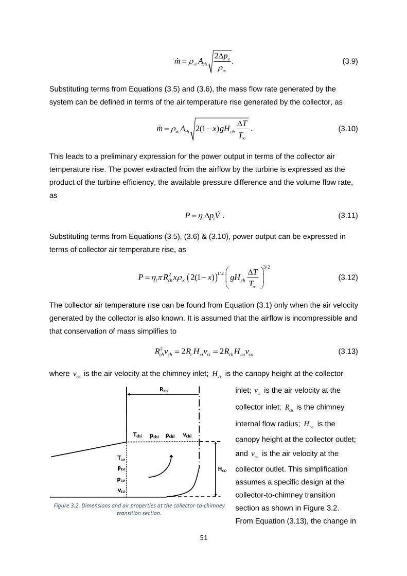
51
2
.vch
pm A
(3.9)
Substituting terms from Equations (3.5) and (3.6), the mass flow rate generated by the
system can be defined in terms of the air temperature rise generated by the collector, as
2(1 )ch ch
Tm A x gH
T
. (3.10)
This leads to a preliminary expression for the power output in terms of the collector air
temperature rise. The power extracted from the airflow by the turbine is expressed as the
product of the turbine efficiency, the available pressure difference and the volume flow rate,
as
t tpVP . (3.11)
Substituting terms from Equations (3.5), (3.6) & (3.10), power output can be expressed in
terms of collector air temperature rise, as
3/2
1/22 2(1 )t ch ch
TR x gP H
Tx
(3.12)
The collector air temperature rise can be found from Equation (3.1) only when the air velocity
generated by the collector is also known. It is assumed that the airflow is incompressible and
that conservation of mass simplifies to
2 2 2ch ch c ci ci ch co cov R H v R HR v (3.13)
where ch
v is the air velocity at the chimney inlet; ci
H is the canopy height at the collector
inlet; ci
v is the air velocity at the
collector inlet; ch
R is the chimney
internal flow radius; co
H is the
canopy height at the collector outlet;
and co
v is the air velocity at the
collector outlet. This simplification
assumes a specific design at the
collector-to-chimney transition
section as shown in Figure 3.2.
From Equation (3.13), the change in
Figure 3.2. Dimensions and air properties at the collector-to-chimney transition section.

52
air velocity across the collector can be expressed in terms of air velocity at the chimney inlet.
Air velocity at the chimney inlet is known in terms of collector temperature difference, as
given in Equation (3.10).
Hence, the change in air velocity across the collector can be expressed in terms of the
collector geometry and the air temperature difference across the collector:
2 2
2(1 ) .2 2 2 2
ch ch ch chch ch
co c ci co c ci
R R R R Tv x gH
H R H H R H Tv
(3.14)
The kinetic energy term of the collector energy balance (Equation (3.1)) is written in terms of
collector air temperature difference as
3/2
21 1
22(
21 )ch chx gH
Tm v A
T
, (3.15)
where is a geometric parameter defined as
2 3 4
2 2 24 2 4
ch ch ch
co c ci co c ci
R R R
H R H H R H . (3.16)
Now that the mass flow rate and collector air kinetic energy are both known in terms of
collector air temperature difference, conservation of energy for the collector (Equation (3.1))
can now be expressed solely in terms of plant dimensions and collector air temperature
difference. Rearranging to make collector air temperature difference the subject, the
following is obtained:
11/2 3/2
23/2
2
2(1 ) 2(1 )c c ch chp
ch
IR x gH x gHT
R T Tc
(3.17)
where is given by Equation (3.16).
Equation (3.17) can be substituted into Equation (3.12) to give an expression for power
output solely in terms of environmental and geometric parameters. Hence,
2
(1 )
t c c ch
p ch
xI R gH
c T gP
x H
(3.18)
can be said to represent a single-equation expression for a simple STC model, useful for
establishing a rough power output very quickly, if the efficiencies of components are known.
Note that while the chimney radius is eliminated from Equation (3.18) (due to its presence in

53
the denominator of Equation (3.17) and the numerator of Equation (3.12)), it is present in the
coefficient .
Figure 3.3. Power output and collector temperature rise for a range of chimney heights simulated by the simple STC model.
Figure 3.4. Power output and collector temperature rise for a range of collector radii simulated by the simple STC model.
Equations (3.17) and (3.18) can be used to simulate STC performance for varying input
parameters, enabling insight to be gained into how the STC plant behaves with different
dimensions. Figure 3.3 and Figure 3.4 show the performance of a reference STC plant (with
dimensions defined in Appendix I) with varying chimney height and collector radius
respectively. Figure 3.3 shows the collector temperature rise falling with increasing chimney
height.
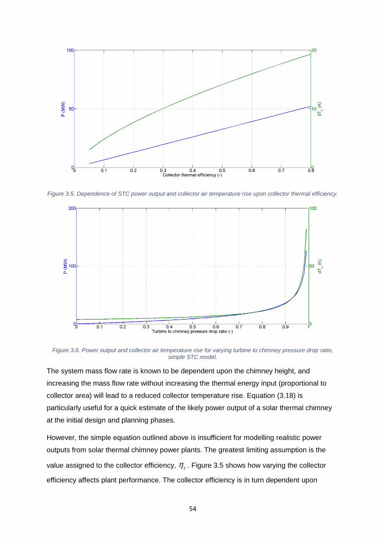
54
Figure 3.5. Dependence of STC power output and collector air temperature rise upon collector thermal efficiency.
Figure 3.6. Power output and collector air temperature rise for varying turbine to chimney pressure drop ratio, simple STC model.
The system mass flow rate is known to be dependent upon the chimney height, and
increasing the mass flow rate without increasing the thermal energy input (proportional to
collector area) will lead to a reduced collector temperature rise. Equation (3.18) is
particularly useful for a quick estimate of the likely power output of a solar thermal chimney
at the initial design and planning phases.
However, the simple equation outlined above is insufficient for modelling realistic power
outputs from solar thermal chimney power plants. The greatest limiting assumption is the
value assigned to the collector efficiency, c . Figure 3.5 shows how varying the collector
efficiency affects plant performance. The collector efficiency is in turn dependent upon
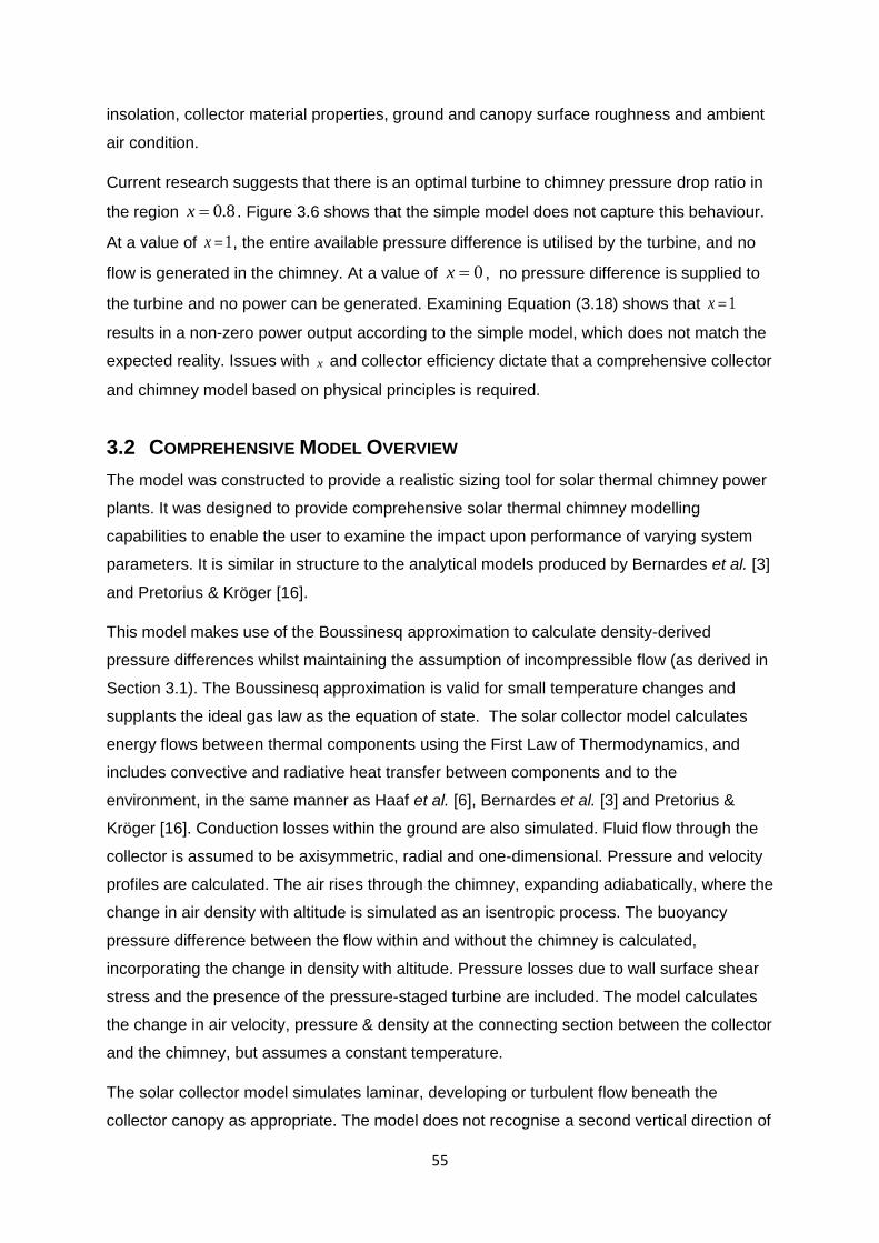
55
insolation, collector material properties, ground and canopy surface roughness and ambient
air condition.
Current research suggests that there is an optimal turbine to chimney pressure drop ratio in
the region 0.8x . Figure 3.6 shows that the simple model does not capture this behaviour.
At a value of 1x , the entire available pressure difference is utilised by the turbine, and no
flow is generated in the chimney. At a value of 0x , no pressure difference is supplied to
the turbine and no power can be generated. Examining Equation (3.18) shows that 1x
results in a non-zero power output according to the simple model, which does not match the
expected reality. Issues with x and collector efficiency dictate that a comprehensive collector
and chimney model based on physical principles is required.
3.2 COMPREHENSIVE MODEL OVERVIEW
The model was constructed to provide a realistic sizing tool for solar thermal chimney power
plants. It was designed to provide comprehensive solar thermal chimney modelling
capabilities to enable the user to examine the impact upon performance of varying system
parameters. It is similar in structure to the analytical models produced by Bernardes et al. [3]
and Pretorius & Kröger [16].
This model makes use of the Boussinesq approximation to calculate density-derived
pressure differences whilst maintaining the assumption of incompressible flow (as derived in
Section 3.1). The Boussinesq approximation is valid for small temperature changes and
supplants the ideal gas law as the equation of state. The solar collector model calculates
energy flows between thermal components using the First Law of Thermodynamics, and
includes convective and radiative heat transfer between components and to the
environment, in the same manner as Haaf et al. [6], Bernardes et al. [3] and Pretorius &
Kröger [16]. Conduction losses within the ground are also simulated. Fluid flow through the
collector is assumed to be axisymmetric, radial and one-dimensional. Pressure and velocity
profiles are calculated. The air rises through the chimney, expanding adiabatically, where the
change in air density with altitude is simulated as an isentropic process. The buoyancy
pressure difference between the flow within and without the chimney is calculated,
incorporating the change in density with altitude. Pressure losses due to wall surface shear
stress and the presence of the pressure-staged turbine are included. The model calculates
the change in air velocity, pressure & density at the connecting section between the collector
and the chimney, but assumes a constant temperature.
The solar collector model simulates laminar, developing or turbulent flow beneath the
collector canopy as appropriate. The model does not recognise a second vertical direction of
56
flow and thus all the fluid within the collector is assumed to be moving at the mean velocity
towards the collector outlet. The heat transfer coefficient governing heat loss to the ground is
assumed to be constant, and is based upon the ground material properties. Other heat
transfer coefficients are based upon phenomenological equations given in Pretorius et al.
[16], in order to obviate the need for finite element methods.
A potential issue with the axisymmetrical radial flow assumption is highlighted by Fasel et al.
[95], where the authors use CFD to show that convection cells evolve in the airflow beneath
the collector canopy and that the flow is thus not radial. Similarly, the ambient wind velocity
is not radial, and ambient wind can destroy radial symmetry of the working air velocity
beneath the collector canopy, as shown by Ming et al. [57]. However, when considering heat
losses due to ambient air flow above the collector canopy, the non-radial nature of the
ambient wind is of no importance, provided the assumption of constant ambient air
temperature is maintained. The magnitude of the ambient air velocity has an effect upon
convective heat losses, but with the assumption that the ambient air represents an infinitely
large heat sink, the ambient air temperature does not change and the direction of the airflow
is therefore of no consequence.
3.3 COMPREHENSIVE ANALYTICAL MODEL STRUCTURE
The comprehensive model has the same essential structure as the simple model, but it has
been developed to simulate the collector from first physical principles (i.e. remove the
assumption of constant collector efficiency) and to include a more accurate method of
calculating the motive pressure difference generated by the chimney.
Solar thermal chimney simulation is a coupled problem, requiring iteration between the
collector and chimney models for a converged solution. The system mass flow rate
determines the velocity profile through the collector, which determines the collector air
temperature rise. The mass flow rate is determined by the buoyancy force in the chimney,
which depends on the collector temperature rise. Hence there is an interdependency
between collector temperature rise and system mass flow rate (Figure 3.7).
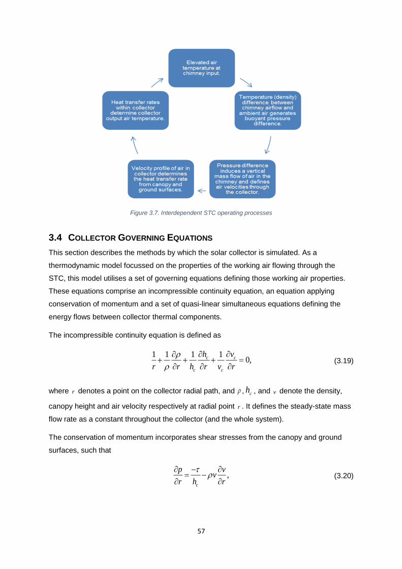
57
Figure 3.7. Interdependent STC operating processes
3.4 COLLECTOR GOVERNING EQUATIONS
This section describes the methods by which the solar collector is simulated. As a
thermodynamic model focussed on the properties of the working air flowing through the
STC, this model utilises a set of governing equations defining those working air properties.
These equations comprise an incompressible continuity equation, an equation applying
conservation of momentum and a set of quasi-linear simultaneous equations defining the
energy flows between collector thermal components.
The incompressible continuity equation is defined as
1 1 1 1
0,c c
c c
h v
r r h r v r
(3.19)
where r denotes a point on the collector radial path, and , ch , and v denote the density,
canopy height and air velocity respectively at radial point r . It defines the steady-state mass
flow rate as a constant throughout the collector (and the whole system).
The conservation of momentum incorporates shear stresses from the canopy and ground
surfaces, such that
,c
p vv
r h r
(3.20)
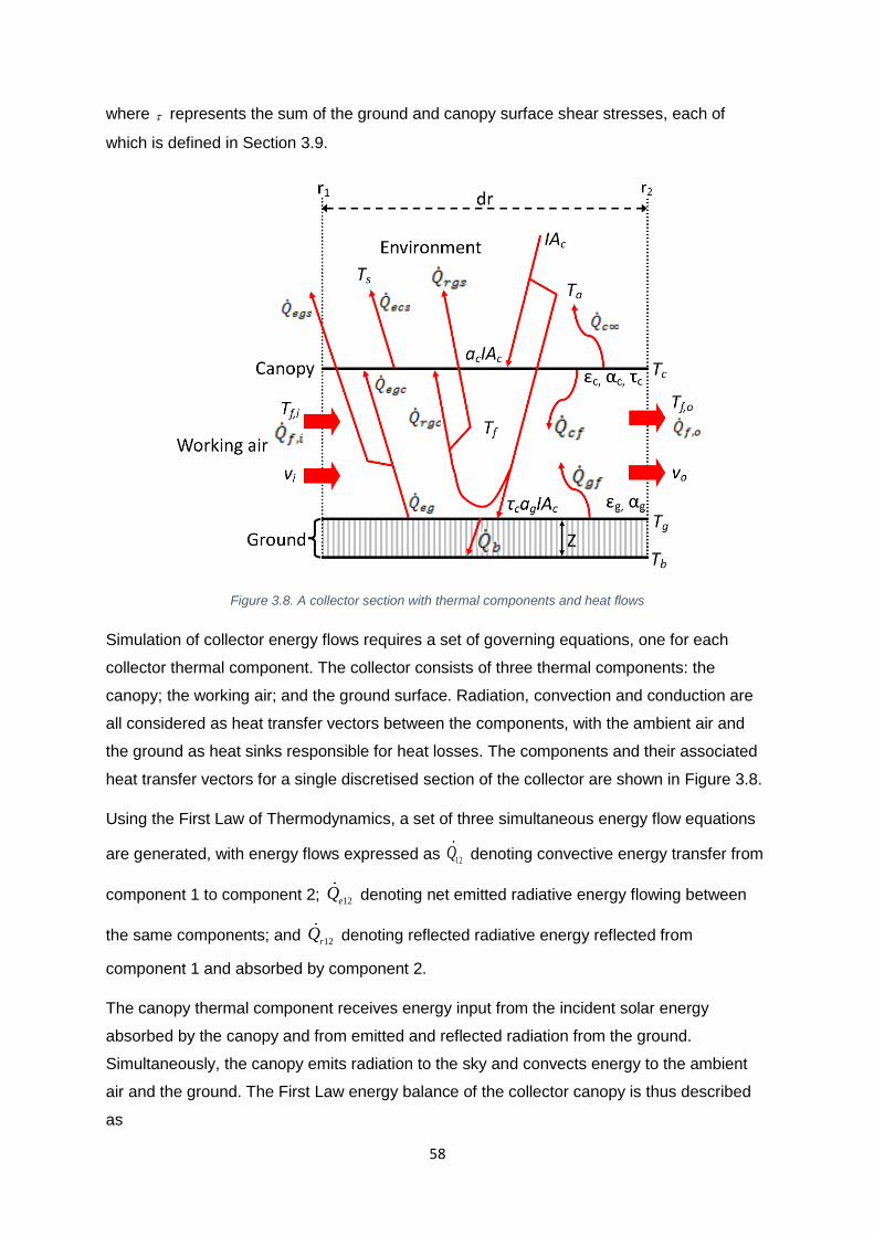
58
where represents the sum of the ground and canopy surface shear stresses, each of
which is defined in Section 3.9.
Figure 3.8. A collector section with thermal components and heat flows
Simulation of collector energy flows requires a set of governing equations, one for each
collector thermal component. The collector consists of three thermal components: the
canopy; the working air; and the ground surface. Radiation, convection and conduction are
all considered as heat transfer vectors between the components, with the ambient air and
the ground as heat sinks responsible for heat losses. The components and their associated
heat transfer vectors for a single discretised section of the collector are shown in Figure 3.8.
Using the First Law of Thermodynamics, a set of three simultaneous energy flow equations
are generated, with energy flows expressed as 12Q denoting convective energy transfer from
component 1 to component 2; 12eQ denoting net emitted radiative energy flowing between
the same components; and 12rQ denoting reflected radiative energy reflected from
component 1 and absorbed by component 2.
The canopy thermal component receives energy input from the incident solar energy
absorbed by the canopy and from emitted and reflected radiation from the ground.
Simultaneously, the canopy emits radiation to the sky and convects energy to the ambient
air and the ground. The First Law energy balance of the collector canopy is thus described
as
59
,c c egc rgc ecs c cfIA Q Q Q Q Q (3.21)
where c the absorptivity of the canopy, I insolation (Wm-2), and c
A collector plan-
view area. The working air flowing through the collector discretised section has thermal and
kinetic energy inputs from the incoming air flow, as well as convected energy from the
ground and canopy surfaces. The convected thermal energy leads to an increase in air
temperature and velocity at the collector outlet. Thus the working air energy balance is
expressed mathematically as
2 2 .2
cf gf p o i
mQ Q mc T v v (3.22)
Some STC designs utilise a canopy with a variation in height along the radial path, changing
the mean height of the working air with radial path position. For the reference STC plant, the
total change of height along the collector radius is 4 m. The associated potential energy has
not been included as its impact is minimal. The ratio of potential energy gain to thermal and
kinetic energy gain through the collector radius is expressed as
2
,
2
pot
T kin
p
Q mgh
vc
Q Qm T
(3.23)
where h is the canopy height difference between collector inlet and outlet; T is the
temperature difference between the collector inlet and outlet; and v is the air velocity at the
collector outlet. The subscript pot denotes potential energy; T denotes thermal energy; and
kin denotes kinetic energy. For the reference STC plant (specified in Appendix I), the ratio of
potential energy to thermal and kinetic energy through the collector is 0.00218, meaning that
the potential energy, disregarded in this model, is only 0.218 % of the thermal and kinetic
energy, which were included in the model. Hence, it can be concluded that the impact of
potential energy is minimal and its exclusion justified.
The ground surface energy balance is characterised by energy inputs from the solar
radiation, transmitted through the canopy and absorbed at the ground surface, as well as
energy outputs in terms of emitted radiation, energy convected to the air and energy
conducted into the ground.
Mathematically, this First Law balance is expressed as
.c g c eg gf bIA Q Q Q (3.24)
60
Where they appear throughout this chapter, subscript denotes ambient air; subscript s
denotes sky (a theoretical parallel plate for radiative heat loss to ambient); subscript c
denotes the canopy; subscript f denotes the working air; subscript g denotes the ground
surface; subscript r denotes a radiative heat transfer coefficient; subscript b denotes ground
heat loss; subscript i denotes inlet; and subscript o denotes outlet. It can be deduced from
Figure 3.8 that the emitted radiation from the ground egQ splits into emitted radiation
absorbed by the canopy, egcQ , and emitted radiation lost to the ambient (sky), egs
Q :
.eg egc egsQ Q Q (3.25)
Contained within Equation (3.25) is an assumption that radiation emitted from the ground
and incident upon the underside of the canopy is either absorbed or transmitted; none of it is
reflected. While the canopy is assumed to have a non-zero reflectivity, this value is low
compared to its absorptivity and transmissivity, and it is omitted here as its impact is minor
and to include it would incur a diminishing loop of radiative reflection between the two
surfaces.
3.5 COLLECTOR DISCRETISATION
The model discretises the one-dimensional flow path (from the inlet at the collector periphery
to the outlet at its centre) into a large quantity of small collector sections. Each discretised
section has an inlet and outlet value for each variable, the inlet values being equal to the
outlet value of the previous discretised section (or, in the case of the first discretised section,
to the ambient environment), and the outlet values of the current discretised section being
calculated using the methods given herein. Investigations into STC performance have shown
the largest change in flow variables at low radial values (close to the collector outlet), as the
reducing flow area of most canopy profiles causes an increase in flow velocity and a drop in
static pressure. In order to maintain the collector model's fidelity, discretisation length is
reduced linearly along the collector length (Figure 3.9). As an example, a collector of radius
2500m discretised into 489 sections has a discretisation length of 19.4m at the inlet and
0.43m at the outlet. It has been established that whilst varying collector discretisation length
along the collector radius is beneficial for model accuracy, having an especially large
number of datapoints for collector discretisation within one simulation is not necessary.
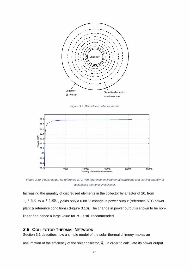
61
Figure 3.9. Discretised collector annuli.
Figure 3.10. Power output for reference STC with reference environmental conditions and varying quantity of
discretised elements in collector.
Increasing the quantity of discretised elements in the collector by a factor of 20, from
500c
n to 10000c
n , yields only a 0.88 % change in power output (reference STC power
plant & reference conditions) (Figure 3.10). The change in power output is shown to be non-
linear and hence a large value for cn is still recommended.
3.6 COLLECTOR THERMAL NETWORK Section 3.1 describes how a simple model of the solar thermal chimney makes an
assumption of the efficiency of the solar collector, c , in order to calculate its power output.
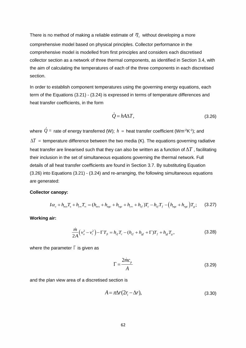
62
There is no method of making a reliable estimate of c without developing a more
comprehensive model based on physical principles. Collector performance in the
comprehensive model is modelled from first principles and considers each discretised
collector section as a network of three thermal components, as identified in Section 3.4, with
the aim of calculating the temperatures of each of the three components in each discretised
section.
In order to establish component temperatures using the governing energy equations, each
term of the Equations (3.21) - (3.24) is expressed in terms of temperature differences and
heat transfer coefficients, in the form
,Q hA T (3.26)
where =Q rate of energy transferred (W); h heat transfer coefficient (Wm-2K-1); and
T temperature difference between the two media (K). The equations governing radiative
heat transfer are linearised such that they can also be written as a function of T , facilitating
their inclusion in the set of simultaneous equations governing the thermal network. Full
details of all heat transfer coefficients are found in Section 3.7. By substituting Equation
(3.26) into Equations (3.21) - (3.24) and re-arranging, the following simultaneous equations
are generated:
Collector canopy:
( ) ;c ecs s c ecs egc rgc c cf c cf f egc rgc gI h T h T h h h h h T h T h h T (3.27)
Working air:
2 2 ( )2
,o i fi cf c cf gf f gf g
mv v T h T h h T h T
A (3.28)
where the parameter is given as
2 pmc
A (3.29)
and the plan view area of a discretised section is
(2 ),iA r r r (3.30)
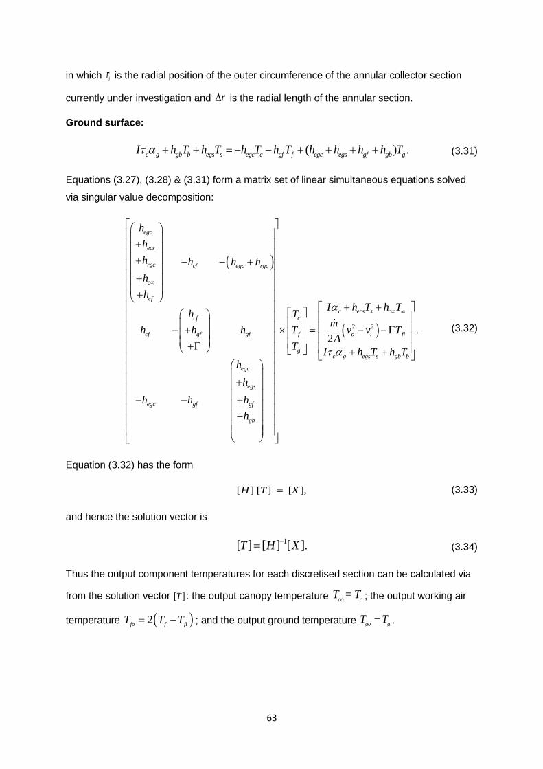
63
in which ir is the radial position of the outer circumference of the annular collector section
currently under investigation and r is the radial length of the annular section.
Ground surface:
( ) .c g gb b egs s egc c gf f egc egs gf gb gI h T T h T h T h h h Th h (3.31)
Equations (3.27), (3.28) & (3.31) form a matrix set of linear simultaneous equations solved
via singular value decomposition:
egc
ecs
rgc cf egc rgc
c
cf
c ecs s ccf c
cf gf gf f
g
egc
egs
egc gf gf
gb
h
h
h h h
h
h
h T h Th T
h h h T
T
h
h h h
h
h
I
h
2 2 .2
o i fi
c g egs s gb b
mv v T
A
I h T h T
(3.32)
Equation (3.32) has the form
[ ] [ ] [ ],H T X (3.33)
and hence the solution vector is
1[ ] [ ] [ ].T H X (3.34)
Thus the output component temperatures for each discretised section can be calculated via
from the solution vector [ ]T : the output canopy temperature =co c
T T ; the output working air
temperature 2fo f fi
T T T ; and the output ground temperature go gT T .

64
3.7 HEAT TRANSFER COEFFICIENTS
The matrix of heat transfer coefficients, [ ]H , must be defined in order for the component
temperatures to be found. This section describes the methods used to determine the heat
transfer coefficients.
For the heat transfer between generic media 1 and 2, any temperature-dependent properties
are calculated at the mean temperature 12mT where:
1 212
2m
T TT
(3.35)
3.7.1 Convective Heat Transfer Coefficient Derivation
The heat transfer coefficients presented herein consist of coefficients for convective heat
transfer (denoted h ) and for radiative heat transfer (denoted rh ). Convective heat transfer
further consists of two related processes. Natural convection is the transfer of heat from a
heated surface to the cooler fluid above by conduction and the subsequent convection of the
heated fluid away from the surface by buoyancy. The velocity due to buoyancy is non-
negligible compared to other forced velocity components. By contrast forced convection is
the process in which heat is conducted to the fluid adjacent to the heated surface, only for
the fluid to be moved by external forced velocities, which are large compared to buoyancy
velocity components.
The combined natural and forced convection heat transfer coefficient takes the form
,h b cv (3.36)
where b is a dimensionless parameter representing natural convection heat transfer; c is a
parameter representing forced convection heat transfer; and v is the free-stream air velocity
of the fluid. Parameters b and c depend upon material temperatures and thermal properties,
and cv and h are dimensionless.
The calculation of natural convective heat transfer coefficients and forced convective heat
transfer coefficients are considered separately before joining them as in Equation (3.36). The
case of a heated horizontal surface facing up is used in the derivation, and alternative
configurations are specified where they apply to the STC collector.
Considering first the heat transfer by natural convection, Bejan [101] has shown it to depend
upon the Nusselt Number and the Rayleigh Number, according to
1/3Nu Ra ,a (3.37)

65
where the Nusselt Number is the ratio of forced convective heat transfer to natural
convective heat transfer; and the Rayleigh Number is associated with natural convection in
the fluid (e.g. it can be used to predict the existence of convective instabilities in the fluid).
For a heated surface (subscript 1) exposed to cooler air (subscript 2), Equation (3.37)
becomes a dimensionless expression for the natural convection heat transfer coefficient:
1/3
2 2
1 2
,( )
mn
p
Ta
g T T c kh
(3.38)
where is the dynamic viscosity of the air and k is the thermal conductivity of the air. A
review of experimental work for constant-temperature heated surfaces validated with
additional experimental work led Burger [103] to conclude that a suitable value for a is
0.2106. Thus the natural heat transfer coefficient is expressed as
1/3
2 2
1 2
0.2106.
( )
n
m
p
T
g T T c k
h
(3.39)
Secondly we consider the forced heat transfer coefficient. The Reynolds-Colburn analogy
states that in the absence of pressure gradients, the momentum and energy boundary layer
equations are analogous, that is: normalised velocity is equal to normalised temperature.
This analogy leads to
Re Nu,2
fC (3.40)
which, upon expanding with the definitions of Reynolds and Nusselt Numbers gives the
forced convection heat transfer coefficient in terms of free-stream flow velocity v as
2/3
.2
f p
w
p
C c v
c
k
h cv
(3.41)
Thus, substituting Equations (3.38) and (3.41) into Equation (3.36) we obtain:
1/3 1/3
2 2
1 2 1 2
0.) 2 (
2)
106 .(
fm m
p
Ch v
T T
T c k g TT Tg
(3.42)
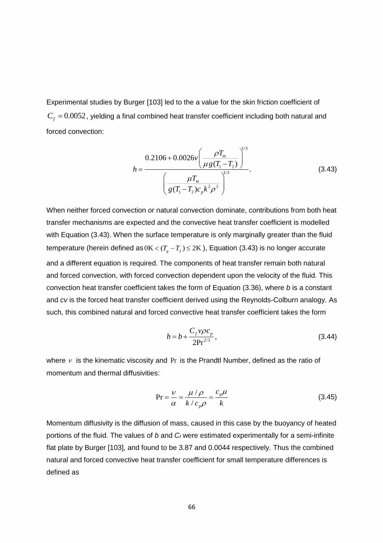
66
Experimental studies by Burger [103] led to the a value for the skin friction coefficient of
0.0052fC , yielding a final combined heat transfer coefficient including both natural and
forced convection:
1/3
1 2
1/3
2 2
1 2
(0.2106 0.0026
(
)
)
.
m
m
p
T
g T T
T
T c
v
h
g T k
(3.43)
When neither forced convection or natural convection dominate, contributions from both heat
transfer mechanisms are expected and the convective heat transfer coefficient is modelled
with Equation (3.43). When the surface temperature is only marginally greater than the fluid
temperature (herein defined as 0K ( ) 2Kg f
T T ), Equation (3.43) is no longer accurate
and a different equation is required. The components of heat transfer remain both natural
and forced convection, with forced convection dependent upon the velocity of the fluid. This
convection heat transfer coefficient takes the form of Equation (3.36), where b is a constant
and cv is the forced heat transfer coefficient derived using the Reynolds-Colburn analogy. As
such, this combined natural and forced convective heat transfer coefficient takes the form
2/3
,2Pr
f pC v ch b
(3.44)
where is the kinematic viscosity and Pr is the Prandtl Number, defined as the ratio of
momentum and thermal diffusivities:
/
r/
Pp
p
c
k c k
(3.45)
Momentum diffusivity is the diffusion of mass, caused in this case by the buoyancy of heated
portions of the fluid. The values of b and Cf were estimated experimentally for a semi-infinite
flat plate by Burger [103], and found to be 3.87 and 0.0044 respectively. Thus the combined
natural and forced convective heat transfer coefficient for small temperature differences is
defined as

67
2/3
3.87 0.0022 .Pr
pv ch
(3.46)
When forced convection dominates, the heat transfer coefficient can be calculated using
Gnielinski's equation for fully-developed turbulent flow [23]:
1223
8
1 1
Re 1000 Pr
Pr2.7 18
g
hg
f
k
df
h
(3.47)
where g
f Darcy friction factor (distinct from the Fanning friction factor) of the ground-
working air interface. The Darcy friction factor is determined by the Colebrook equation for
turbulent flow and a simple relationship dependent upon the Reynolds Number for laminar
flow. See Section 3.9 for more details.
In the cases where the fluid temperature exceeds the surface temperature, i.e. 1 20T T ,
Equation (3.46) gives the heat transfer coefficient. In the trivial case whereby the ground and
working air temperatures are equal, no heat transfer takes place.
3.7.2 hgf - Ground - Working Air Convective Heat Transfer Coefficient
Under normal operating circumstances, the ground – working air interface is accurately
simulated as a semi-infinite heated surface facing up, over which flows a cooler fluid. The
dominant heat transfer mechanism will determine the rate of heat transfer between these
media. As such, the value of gf
h is determined by selecting the greatest of the values
returned by Equations (3.43), (3.46) and (3.47).
3.7.3 hcf - Canopy - Working Air Convective Heat Transfer Coefficient
When c f
T T , the canopy is modelled as a heated surface facing down. Since buoyancy
forces ensure that heated air remains against the lower canopy surface until swept away by
the velocity of the air, it is assumed that heat transfer takes place by forced convection only,
and as such Equation (3.47) is deployed. This equation also includes the effect of surface
roughness on heat transfer and thus is fully suitable for modelling this heat transfer scenario.
When c f
T T , the canopy is now modelled as a cooled surface facing down and in this
scenario the air immediately adjacent to the lower surface of the canopy is cooled and falls
due to its negative buoyancy. This is a form of natural convection. It is possible that this form

68
of natural convection dominates when working air velocities are low, but higher velocities will
cause forced convection to dominate. Thus, as with Section 3.7.2, the dominant heat
transfer mechanism is selected and the greatest heat transfer rate calculated by Equations
(3.43), (3.46), and (3.47) is used. Note that a cooled surface facing down is analogous to a
heated surface facing up and thus the same set of equations can be used to calculate the
heat transfer equations for both scenarios.
3.7.4 hc∞ - Canopy – Ambient Air Convective Heat Transfer Coefficient
When c
T T
, the canopy is modelled as an upward-facing heated surface. Depending on
the ambient wind velocity w
v , the dominant convective heat transfer mechanism may be
natural convection, forced convection, or neither may dominate. As such, Equations (3.43),
(3.46), and (3.47)are suitable for calculating the heat transfer coefficient for the interface
between the canopy and the ambient air, when the air velocity v is replaced with the
ambient wind velocity w
v .
Note that in the model presented herein, this assumes that the atmosphere is an infinitely
large heat sink (i.e. the ambient air temperature does not change, despite heat input), and
thus the direction of ambient air velocity across the canopy surface does not change heat
losses to ambient. As explored earlier in the chapter, the assumption of constant ambient air
temperature means that only the magnitude and not the direction of ambient air velocity
affects the collector’s performance. To remove this assumption would increase model
complexity substantially, as it would require the creation of a domain above the canopy
surface, within which the ambient air temperature would be calculated, limited by assumed
conditions at the domain’s boundary. This would increase computational effort significantly,
and for this reason the assumption of constant-temperature ambient wind has been made. If
there is no wind velocity (-1
0msw
v ), the greatest of Equations (3.43) and (3.46) is used,
with the second term of each equation being equal to zero.
3.7.5 hgb - Ground Heat Conduction Coefficient
gT is strictly the temperature at the ground surface. Some heat is lost by conduction into the
ground. In order to include this heat loss in the model, it was assumed that the temperature
underground was constant at depth Z . The appropriate equation for the heat transfer
coefficient was determined to be [3]:
,2,
12
g g p g
gb
k ch
(3.48)

69
where the denominator is equal to t , and t is the solar hour from solar midnight. By
setting t=12, the model calculates heat loss at solar noon, with the greatest heat flux incident
upon the ground surface.
3.7.6 Radiative Heat Transfer Coefficients
The STC collector includes two different forms of radiative heat transfer. The first calculates
net radiative heat transfer between the surfaces of two solid components within the collector,
whilst the second calculates a theoretical ``clear-sky temperature'' which allows one to
calculate the rate of heat radiated to the environment. The net radiated heat between
surfaces 1 and 2 is calculated as follows:
4 4
1 212
1 2
( )
1 11
T TQ
(3.49)
Where material emissivity and Stefan-Boltzmann Constant. However, for the net
radiated heat to be calculated within the matrix inversion framework laid out in Section 3.6,
the equation calculating rate of heat transferred needs to be linearised into the form
1212 1 2( ).r
Qh T T
A (3.50)
Equation (3.49) is divided by 1 2T T to give the heat transfer coefficient for net radiated
heat:
2 2
1 2 1 212
1 2
( )( ).
1 11
r
T T T Th
(3.51)
Equation (3.51) is thus a heat transfer coefficient for net radiated heat between two parallel
plates. Applied to the radiated heat between ground and canopy, it takes the form of
Equation (3.51), with temperatures 1T and 2T exchanged for gT and cT .
The calculation of heat radiated from the collector canopy to the ambient requires a
temperature for a theoretical parallel plate representing the ambient environment. This is
called the “clear-sky temperature”, and is defined as
5 2 1/4273.15 ( 273.15)(0.711 0.0056 7.3 10 0.013cos(15 )) ,s dp dpT T T T t
(3.52)
70
where t is the solar hour from midnight (Bernardes et al., [3]), and the dew-point temperature
dpT is expressed as
237.7
.17.271
dpT
(3.53)
The parameter is defined as
17.271( 273.15)
ln( ),35.45
RH
T
T
(3.54)
in which RH
is the relative humidity of the atmospheric air. Now that the clear-sky
temperature is known, the heat transfer coefficient for radiated heat lost to the environment
from the canopy surface can be calculated:
2 2
1 1 1 1
1
( )( )( ).s s s
rcs
T T T T T Th
T T
(3.55)
3.8 COLLECTOR AIR FLOW
This section calculates the air velocity, pressure and density profiles through the collector for
a given mass flow rate. The air temperature is calculated in Section 3.6. Further details
regarding collector air pressure profiles are given below.
The working air pressure, velocity and density is calculated for each discretised collector
section. All the input variables (subscript 1) are known, whilst the output variables (subscript
2) are unknown. Each discretised section's output variables become the input variables of
the subsequent section. The output density is calculated using the Boussinesq
approximation:
2 1
2 1
1
1f f
f
T T
T
(3.56)
The assumption that density is not a function of pressure also prevents pressure being a
function of density, i.e. it removes any relationship of state between them such as that
supplied by the ideal gas law. Therefore air velocity is not affected by pressure difference as
it is in the chimney (see Section 3.11), but is affected by air temperature. Hence it is a
problem in two variables, density and temperature, and must be solved with two equations,
those being mass conservation,

71
1 1 12
2 2
A vv
A
(3.57)
and energy conservation (Equation (3.22)). Section 3.6 gives details of how the working air
energy equation forms part of a network of thermal components connected by different heat
transfer mechanisms. As such, Equations (3.57) and (3.22) cannot be solved in isolation, as
they each form part of a wider set of equations. In the model implementation, each set of
equations is solved iteratively, with air velocity being the common variable. All variables are
updated on each iteration and the iterative process ends when the air velocity at the
discretised section outlet ceases to change significantly from one iteration to the next.
Collector air pressure is determined by airflow momentum balance, derived from a
discretised version of Equation (3.20):
2 12 1 1 1 2 1
2
( )( ),
c
r rp p v v v
H
(3.58)
where is the sum of the collector surface shear stresses, calculated in Section 3.9.
3.9 SURFACE SHEAR STRESS
This section details the calculation of surface shear stresses for the collector and chimney
components. Regardless of flow regime (laminar, transitional or turbulent), the drag force
due to shear stress at point x along a fluid flowing parallel to a flat plate of width b is given by
0
(( ) .)
x
xD x dxb (3.59)
Differentiating, this yields
.dD
bdx
(3.60)
The drag force on a parallel plate was derived by von Kármán [104] as
2( ,)D x bU (3.61)
in which U is the free-stream velocity and is a quantity termed “momentum thickness”,
defined by the fluid velocity profile through the boundary layer:
0
1 ,u u
U Udy
(3.62)

72
where ( )u y is the fluid boundary layer velocity at height y within the boundary layer. Note at
y , u U . Differentiating Equation (3.61) and substituting into Equation (3.60) yields an
expression for shear stress in terms of free-stream velocity and momentum thickness:
2 .
dU
dx
(3.63)
However, the momentum thickness still requires knowledge of the flow velocity profile ( )u y
within the boundary layer. Rearranging Equation (3.63) into non-dimensional form yields the
skin friction coefficient for flow over a horizontal flat plate, as
2
.2
fc d
dx U
(3.64)
Alternatively, it yields the Darcy friction factor for flow between two parallel plates as
2
.8
d d
dx
f
U
(3.65)
Thus, depending on the appropriate solution for the flow and surface(s) under consideration,
the surface friction shear stress is
2
2
fcU (3.66)
for flow over a horizontal plate, and
2
8
df U (3.67)
for flow between two parallel plates.
Constant skin friction coefficients are used based on experiments undertaken by Burger
[103], with values given in Section 3.7. The Darcy friction factor is calculated using the
implicit Colebrook equation when turbulent flow is present [105]:
1 2.51
2log7.4 Re
r
cd d
e
Hf f
(3.68)
where roughness lengthr rg
e e for the ground surface and r rc
e e for the canopy surface. The
implicit nature of the Colebrook equation requires an iterative numerical solution. When the
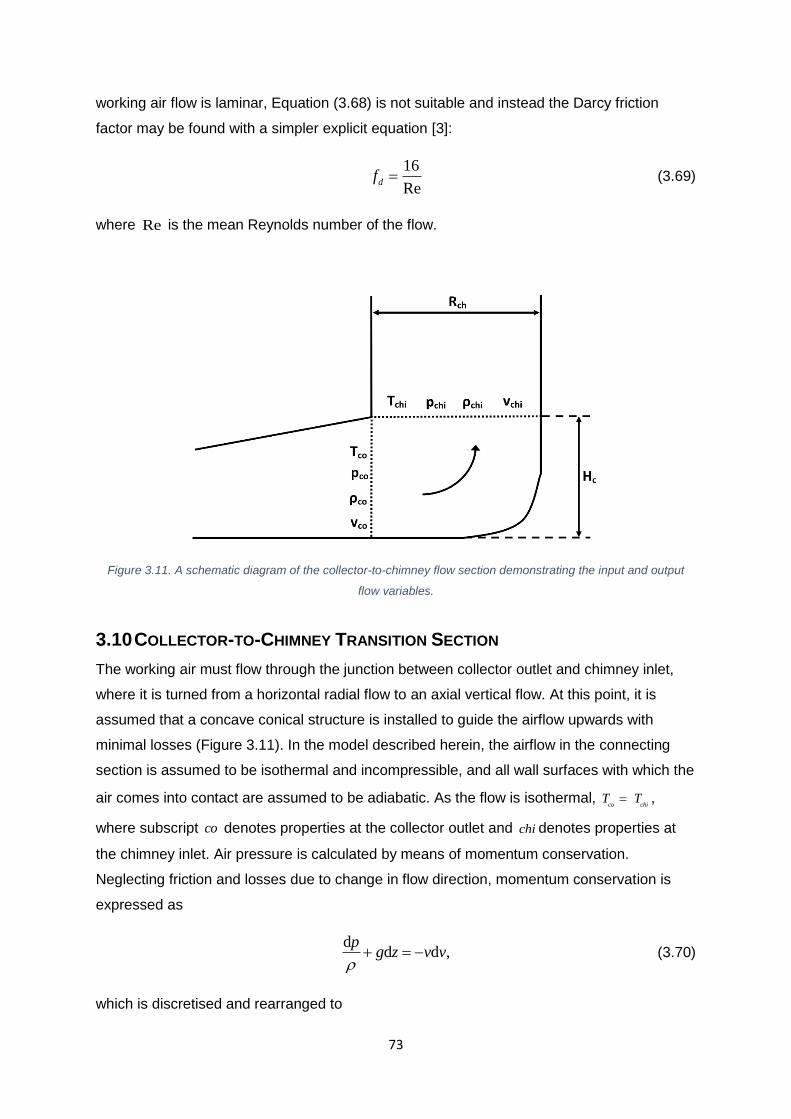
73
working air flow is laminar, Equation (3.68) is not suitable and instead the Darcy friction
factor may be found with a simpler explicit equation [3]:
16
Redf (3.69)
where Re is the mean Reynolds number of the flow.
Figure 3.11. A schematic diagram of the collector-to-chimney flow section demonstrating the input and output
flow variables.
3.10 COLLECTOR-TO-CHIMNEY TRANSITION SECTION
The working air must flow through the junction between collector outlet and chimney inlet,
where it is turned from a horizontal radial flow to an axial vertical flow. At this point, it is
assumed that a concave conical structure is installed to guide the airflow upwards with
minimal losses (Figure 3.11). In the model described herein, the airflow in the connecting
section is assumed to be isothermal and incompressible, and all wall surfaces with which the
air comes into contact are assumed to be adiabatic. As the flow is isothermal, co chi
T T ,
where subscript co denotes properties at the collector outlet and chi denotes properties at
the chimney inlet. Air pressure is calculated by means of momentum conservation.
Neglecting friction and losses due to change in flow direction, momentum conservation is
expressed as
d
d d ,p
g z v v (3.70)
which is discretised and rearranged to
74
( ) ( ),chi co chi co co chi cop p g z z v v v (3.71)
where, due to incompressibility, density is constant (chi co
); the mean height of the
flow at the collector outlet and chimney inlet is denoted co
z and chi
z respectively. The
difference in mean flow heights is defined as ( )2
co
chi co
Hz z .
The chimney inlet mean flow velocity chi
v remains unknown and is expressed in terms of
mass conservation:
.cochi co
chi
Av v
A (3.72)
The outlet collector area has a radius equal to the chimney internal flow radius ch
R , and a
height equal to the collector canopy height co
H . As such, the ratio of collector output area to
chimney inlet area can be expressed as
2
.co co
chi ch
A H
A R (3.73)
Substituting Equations (3.72) and (3.73) into Equation (3.71) gives
2 2
1 ,2
co cochi co co
ch
gH Hp p v
R
(3.74)
where p pressure; density; v velocity; co
H outlet collector canopy height; and
chR internal chimney radius.
Within the collector-to-chimney transfer section, most STC designs include some form of
revolute conical structure to direct the airflow from horizontal radial flow to vertical axial flow
with minimum associated pressure losses. Kirstein & Backström [106] studied the impact
upon air pressure and flow exit angle of different conical flow guides within the collector-to-
chimney transition section. They found that the pressure loss coefficient; that is, the pressure
loss ratio between inlet and outlet of the collector-to-chimney transition section, is equal to
0.0558 in the best configuration they evaluated. The worst-performing configuration
delivered a loss coefficient of 0.1060. Since the loss coefficient is low, the current model as
described above does not include loss coefficients. Similarly, surface shear stress due to
wall friction is neglected in this section of the STC simulation. The magnitude of the impact
75
of wall friction has already been shown to be small (see Section 3.8), even across large
distances (i.e. collector radius).
It should be noted that a chimney inlet velocity is implied in Equation (3.72), but this is not
the chimney inlet velocity utilised by the model to define the mass flow rate (as this is the
function of the chimney - see Section 3.11). The STC model structure is such that the
pressure, density and temperature of the airflow at the collector exit are taken forward (via
the collector-to-chimney section) to the chimney inlet, but the air velocity is not. This is
because the chimney generates the air velocity at the chimney inlet, dependent upon the
pressure difference generated by the buoyancy of the warm air within the chimney. The
model iterates until the difference between the mass flow rate generated by the chimney and
the mass flow rate in the collector which feeds the heated air to the chimney is negligibly
small.
3.11 CHIMNEY MODEL
This section describes the model of the chimney component. Like the collector, the chimney
is discretised into sections. Unlike the collector, these sections are uniform, as there is no
change in flow area and therefore no rapid change in flow properties which would warrant
reduced discretisation sizes. The chimney walls are adiabatic and all changes to gas state
variables are assumed to occur through a process of isentropic expansion.
The chimney generates an updraft of air due to the buoyancy of the heated air flowing within
it. More accurately, the buoyancy creates a pressure difference, and the pressure difference
drives the airflow. This model calculates the buoyancy pressure difference profile, and
incorporates the effect of changing density with altitude. Velocity, pressure, temperature and
density of the airflow are all calculated. Unlike the collector, the airflow in the chimney is
driven solely by the buoyancy pressure difference. This means that air velocity can be
defined in terms of pressure difference and this in turn permits the model to simulate the
impact of surface shear stress upon both the pressure and velocity of the flow. The
buoyancy pressure difference is the only motive force, and it is attenuated by both the
pressure loss due to surface shear stress and the pressure loss due to the presence of the
turbine.
3.11.1 Buoyancy Pressure Difference
In order to calculate the buoyancy pressure difference, it is first necessary to establish the
density profiles across the chimney's altitude for both the ambient air and the working air
within the chimney. This is done according to a method laid out by Bernardes et al. [3],
wherein the change in density is assumed to be a process of isentropic expansion. Pressure

76
and temperature profiles for both ambient and working air are created in a similar way. The
density profiles are expressed as
1
11( ) (0) ,1z z
X
(3.75)
in which for convenience an additional parameter is defined as
(0)
.RT
Xg
(3.76)
In the case of the ambient air outside the chimney, 1.235
[3] and the temperature
and density of air at ground level are respectively (0) (0)T T
and (0) (0)
. For the air
within the chimney, 1.4005ch
[3] and the temperature and density of air at ground
level are respectively 0 0ch
T T and (0) (0)ch
.
The general equation for buoyancy pressure difference is as follows:
0
( )dchH
b ch
H
p g z (3.77)
where 0
H the lowest point of updraft under consideration and ch
H height of the chimney
outlet. Substituting Equation (3.75) into Equation (3.77) with the appropriate constants for
both ambient and working air, the following is obtained:
0 0
11
11 11(0) 1 d (0) 1 d .
ch chch
H H
chb ch
ch chH H
p g z z g z zX X
z
(3.78)
Performing the integration leads to the following:
0
0
(0 1 1
1 ,
)
0 1( )
ch ch
chb
chch ch
ch ch ch ch
H Hp gX
X X
H HgX
X X
(3.79)
with X given in Equation (3.76); and
.1
(3.80)

77
Note that, as with Equation (3.76), Equation (3.80) has two values depending on whether the
constants used are those pertaining to the ambient air ( ,
etc.) or to the working air ( ,ch
etc.).
For each discretised chimney section, a new value for buoyancy pressure difference is
calculated, whereby 0
H is the height of the current discretised section output and ch
H
remains constant as the height of the chimney outlet. In this way, the model accounts for the
reducing buoyancy pressure difference with height: As the model advances up the chimney,
through the discretised chimney sections, it is only the remaining portion of the chimney
above the current section which can impose a pressure difference upon the air at that point.
Thus, from the base of the chimney, the whole height of the chimney (minus the mean height
of the air mass at the chimney inlet) is used in calculating the available pressure difference
to drive system mass flow rate.
3.11.2 Chimney Friction
Airflow friction with the chimney walls counteracts the motive buoyancy pressure difference,
reducing the motive force of the chimney. As the chimney airflow is pressure-driven, it
requires iterative calculations of chimney air velocity and pressure drop due to surface shear
stress at discretised steps along the chimney length. This iterative process is explored in
Section 3.11.3. In order to calculate pressure loss due to friction, the chimney must be
discretised into sections. Assuming that the inlet velocity at each section is known and the
Reynolds Number and Darcy friction factor have been calculated, the friction pressure drop
across one discretised section is calculated by assuming it is the same as pressure loss in
standard pipe flows:
2dd
4f ch
ch
zp v
R (3.81)
where dz height of the discretised collector section (m) and ch
v is the chimney air velocity
at the inlet of the current discretised section.
3.11.3 Chimney Pressure & Mass Flow Rate
This section calculates the total pressure drop across the chimney, including that of the
turbine, which then defines the mass flow rate for the whole system. With the Boussinesq
approximation for small changes in air density, the system mass flow rate takes the
incompressible form:
(0) ,(0)c chchhm A v (3.82)
78
The air velocity at the chimney inlet (0)ch
v is defined as:
2
(0)(0)
d,ch
v
ch
pv
(3.83)
where d vp is the pressure drop available to induce an updraft air velocity at the chimney
inlet. d vp is defined as
d (1 )(d d ),v b fp x p p (3.84)
where x is the turbine pressure drop ratio. In other words, the ratio of turbine pressure drop
to the chimney pressure drop:
d
.d d
t
b f
px
p p
(3.85)
Various studies have used values between 0.6x and 0.85x [4,7,8]. An investigation
into the optimum turbine pressure drop ratio has established that the value is not constant
but varies with pressure drop across the chimney and volume flow rate through the turbine
[42]. The model is steady-state, and thus only a constant value can be used. Further work
may well lead to the development of an optimised non-constant turbine pressure drop ratio in
time-linked steady or unsteady simulations, although Bernardes & Zhou [107] showed that
optimum turbine pressure drop ratio does not vary with insolation.
Once the pressure drop available to generate working air velocity is known (Equation (3.84)),
it is utilised to re-evaluate the chimney inlet air velocity (Equation (3.83)) and thus the
pressure drop due to friction (Equation (3.81)) and the mass flow rate (Equation (3.82)). This
loop is iterated whilst the following criterion remains true:
( ) ( 1)
( ),
j j
j
m m
m
(3.86)
where is the convergence value, set at 4
1 10
. The model also performs a mass
continuity check using Equation (3.82) to ensure that continuity is maintained throughout the
model.
3.11.4 Chimney Thermal Performance
This model expressly assumes that the chimney airflow is adiabatic, i.e. no heat is lost from
the working airflow into the chimney walls. A simple calculation of rate of heat transmission
through concrete can test the validity of this assumption. We assume that the chimney walls
79
are built from concrete, which has a thermal conductivity no greater than 1 1
Wm2.5 Kk
,
and that the chimney is of the reference dimensions outlined in Appendix I, with a uniform
wall thickness of 0.05 m. Structural requirements would dictate a thicker non-uniform wall
thickness, but by assuming a thin wall thickness, we test the worst-case scenario with the
greatest heat loss. The rate of heat loss loss
Q across a temperature gradient f
T T T
is
given by
,loss
kA TQ
x
(3.87)
where A is the surface area across which the temperature gradient is applied; and x is the
thickness of the material through which the temperature gradient is applied. For the
reference STC plant, the rate of heat loss is T
1.51MWloss
Q . Assuming a conservative
chimney air velocity of -1
10msv , again to put forward the worst-case scenario, the total
thermal energy in the chimney airflow is
T374 .0MWT pQ mc T (3.88)
The ratio of heat loss to total thermal energy in the flow / 0.0004loss T
Q Q , and thus the heat
loss through a concrete chimney can safely be said to be negligible and the airflow adiabatic.
Different construction materials, such as industrial fabric envelopes as explored in Chapter
6, may require this assumption to be re-visited.
3.12 TURBINE MODEL
For an enclosed quantity of incompressible fluid with a fixed volume, the work which the fluid
is capable of doing is defined by the fluid’s change in pressure:
.E pV (3.89)
For a flowing fluid such as the working air within the STC, the same relation holds. The rate
of work which the fluid is capable of doing depends upon the pressure difference across the
turbine(s) and the volume flow rate through the turbine(s):
,t t t vi i chP pV x p v A (3.90)
where t turbine and powerblock efficiency. It should be noted that the turbine required
for STC power generation is not the same as the standard velocity-staged wind turbine. It is
in fact similar to pressure-staged hydro-electric turbines. This means that the Betz limit for
80
the extraction of mechanical power from fluid flow does not apply. Pressure-staged turbines
possess a particular advantage over velocity staged turbines: Their performance is more
stable and predictable. For pressure-staged turbines, power output varies linearly with
velocity across the turbine blades. For velocity-staged wind turbines, power output varies
with the cube of velocity, meaning small changes in wind velocity can result in large changes
in power output. The stability of pressure-staged turbines is important when considering
security of supply.
3.13 COMPREHENSIVE ANALYTICAL MODEL STRUCTURE
The model presented herein was implemented in Matlab. Solving STC fluid properties and
component temperatures for given dimensions and ambient conditions represents a non-
linear problem which is solved via iteration towards a convergence criterion, of the form
given by Equation (3.86). The STC collector model solves for working air temperature and
pressure, given a mass flow rate of air through the collector. The chimney model generates
a mass flow rate of air, given the condition of the working air at the chimney inlet
(temperature & pressure). Hence, the collector and chimney models iterate until the mass
flow rate and collector outlet temperature values cease to vary appreciably from one iteration
to the next. At this point the collector and chimney flow profiles for all the working air flow
properties advance to the calculation of power output and the simulation ends.
Within the collector and chimney models, there are several sub-models, organised as shown
in Figure 3.12. The collector section model manages further iteration between the
momentum and energy models to ascertain the correct outlet air velocity for the section in
question, as the air velocity features in both the momentum and energy models. Each model
receives its inputs from its parent and returns its outputs to its parent. The model process
runs from left to right of Figure 3.12, ending with the power output calculated based on the
simulated air flow through the specified STC plant.
3.14 STC MODEL VALIDATION
This section details the validation exercises carried out to validate the solar thermal chimney
model described above. The model was based on modelling methods described by
Bernardes et al. [3] and Pretorius et al. [16]. The STC model described herein has been
found to satisfy continuity and conservation of momentum, and has been tested for a wide
range of environmental conditions and plant dimensions.

81
Figure 3.12. STC model & sub-model hierarchy
The use of the Boussinesq approximation was found to lead to a difference compared to the
Ideal Gas behaviour of five orders of magnitude less than the temperature rise itself, and
thus is justified. The energy balance for the complete collector was satisfied with a relative
error of less than 0.1% and the energy balance for the airflow (thermal energy in minus
thermal and kinetic energy out) was found to be accurate to less than 0.001%.
Pretorius & Kröger [16] provide comprehensive performance data, against which this model
has been tested. It was found to conform to the performance trends established by Pretorius
& Kröger; and it performed to within 16% of their model, and within the parameters
established by Bernardes, Backström & Pretorius [20], in their comparison between their two
comprehensive models.
For a plant of the same reference dimensions as those used in this paper, Schlaich et al.
(2004) predicted a power output of 100 MW and Fluri et al. (2009) predicted a power output
of 66 MW. The model presented herein predicts a power output of 63 MW. In the absence of
defined environmental parameters from Fluri et al. (2009) - the authors were conducting a
study of power output over a year - it was assumed that insolation I = 900 Wm−2 and ambient
temperature T∞ = 305 K, representative of a desert environment. Table 3.1 shows the
comparison of performance between models created by Schlaich [12], Bernardes et al. [3],
Fluri et al. [4] and the model detailed within this report.
Performance data from the Manzanares STC prototype was extracted from Haaf (1984),
along with available data on ambient temperature, insolation and material properties. For this
data the simulated power output ranged from 22 kW to 38 kW, across a range of insolation
values from 830 Wm−2 to 1010 Wm−2 and ambient temperature from 293 K to 305 K. This
was up to 5 % less than the recorded power outputs from the Manzanares prototype,
demonstrating that the model presented herein delivers an accurate but conservative
estimate of power output.
Collector
discretisation
Chimney
discretisation
Collector-to-
chimney
transition section
model
Chimney
model
Power
output
calculation
Collector
momentum model
Heat transfer
coefficient model
Matrix solution of
thermal component
temperatures
STC Model
Collector model
Collector section model
Collector energy model
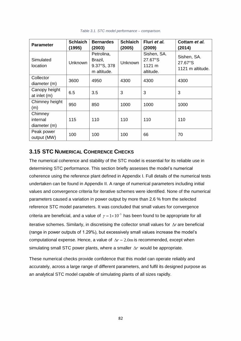
82
Table 3.1. STC model performance – comparison.
Parameter Schlaich
(1995)
Bernardes
(2003)
Schlaich
(2005)
Fluri et al.
(2009)
Cottam et al.
(2014)
Simulated
location Unknown
Petrolina,
Brazil,
9.37°S, 378
m altitude.
Unknown
Sishen, SA.
27.67°S
1121 m
altitude.
Sishen, SA.
27.67°S
1121 m altitude.
Collector
diameter (m) 3600 4950 4300 4300 4300
Canopy height
at inlet (m) 6.5 3.5 3 3 3
Chimney height
(m) 950 850 1000 1000 1000
Chimney
internal
diameter (m)
115 110 110 110 110
Peak power
output (MW) 100 100 100 66 70
3.15 STC NUMERICAL COHERENCE CHECKS
The numerical coherence and stability of the STC model is essential for its reliable use in
determining STC performance. This section briefly assesses the model’s numerical
coherence using the reference plant defined in Appendix I. Full details of the numerical tests
undertaken can be found in Appendix II. A range of numerical parameters including initial
values and convergence criteria for iterative schemes were identified. None of the numerical
parameters caused a variation in power output by more than 2.6 % from the selected
reference STC model parameters. It was concluded that small values for convergence
criteria are beneficial, and a value of 5
1 10
has been found to be appropriate for all
iterative schemes. Similarly, in discretising the collector small values for r are beneficial
(range in power outputs of 1.29%), but excessively small values increase the model’s
computational expense. Hence, a value of 2.0mr is recommended, except when
simulating small STC power plants, where a smaller r would be appropriate.
These numerical checks provide confidence that this model can operate reliably and
accurately, across a large range of different parameters, and fulfil its designed purpose as
an analytical STC model capable of simulating plants of all sizes rapidly.

83
4 SOLAR THERMAL CHIMNEYS: PARAMETRIC
INVESTIGATIONS
Many factors affect the performance of STC power plants. Chief among them are the STC’s
ambient conditions and its dimensions. This chapter presents analyses undertaken to
assess the performance of STCs of different dimensions and under different conditions. By
so doing, this chapter highlights and explores important relationships between the different
variables which affect STC performance. It seeks to investigate systematically the factors
which determine STC performance for future STC researchers and engineering designers
which will simplify the process of designing a STC suited to the constraints of the project,
factors such as location, budget, and technical limitations on chimney height. From this
investigation a series of guiding design rules will be created. The investigations consist of
parametric studies of STC response to different dimensions or environmental parameters,
including surface shear stress in both the collector and chimney components, and turbine
pressure drop ratio.
Section 2.13 details the present state-of-the-art for the process of selecting STC component
dimensions, as well as identifying gaps in the knowledge, specifically that while some
optimisation schemes for STC dimensions have been created (e.g. Gholamalizadeh et al.
[72]; Dehghani & Mohammedi [73]), the optimisation schemes are often based on simplified
STC thermodynamic models and the thermo-fluid mechanisms which determine the matched
dimensions have not been studied fully. By carrying out such a study, it is hoped that further
light can be shed on the limits of STC performance and on the physics of matched
dimensions, as well as providing future STC researchers with a set of design rules which can
guide future STC design work. Existing work by the authors cited above has focussed on the
optimisation procedure and utilised relatively simple STC models, generally without a
discretised thermal network in the collector. The present work introduces a comprehensive
steady-state STC model simulated across a domain of different STC parameters, from which
the best-performing configurations can be identified. Where previous works have identified
optimum configurations, the present work seeks to identify and interrogate best-performing
configurations, understanding the physical mechanisms which lead to certain configurations
out-performing others. Furthermore, multi-criteria optimisation studies in which chimney
height is a variable will always optimise the chimney height at the upper bound of the study.
However, technical and economic factors may limit the achievable chimney height for each
individual project. Using the analytical approach described herein, best-performing
84
configurations can be established for plants of varying chimney height (in this case,
100 0005ch
H mm ).
For the proposed design rules to have credibility, it is important that additional variables
which may affect performance are identified and tested. If they are found not to affect
performance significantly, they can be disregarded for the dimension-matching analysis. For
this reason, we begin by assessing the role of air-surface friction in both the collector and the
chimney and the mechanisms through which it affects plant performance (Section 4.1). It
should be noted that model validation for such a large structure can only be undertaken by
comparing performance data produced by different models.
The ratio of turbine pressure drop to total chimney pressure drop determines the power
available to the turbine and generator block and the mass flow rate of air through the STC.
Much has been published on this topic (see Section 2.6.3), with more recent publications
agreeing that the optimum turbine pressure drop ratio, denoted , has a value in the range
and is relatively insensitive to changes in insolation [107]. Section 4.2 has
expanded this analysis to consider changes in ambient temperature and plant dimensions
and their impact upon optimum x . A sensitivity analysis is presented in Section 4.2, in which
the performance of the reference STC is tested when each of the major environmental and
structural parameters is varied. This serves as an aid to the reader’s understanding of the
behaviour of the STC system, and as a useful check against expected outcomes available in
literature.
Section 4.4 presents an investigation into STC dimension matching. Recognising that
selecting a configuration of best-performing STC dimensions requires an additional non-
physical constraint (typically cost – see Gholamalizadeh et al. [72]), and recognising also
that comprehensive cost models are complex and introduce many additional variables which
may cloud the analysis (as an example, the most comprehensive produced to date is
presented by Fluri et al. [4]), this analysis proposes a different approach. A series of
dimension-matching investigations are carried out for STCs with three different chimney
heights ( 500ch
H m , 750ch
H m , 1000ch
H m ), and a wide range of chimney radii and
collector radii. The collector canopy profile is not varied (see Chapter 5 for a comprehensive
analysis). The physical processes underlying the matched dimensions are studied. This
approach permits the identification of the best-performing dimensions for STCs at a range of
scales, as well as providing insight into the physical processes which led to them, all of
which enables future STC researchers and designers to be better informed about
appropriate STC dimensions for a range of scenarios. Arguably more crucially, this tool
permits the identification of sets of dimensions which are not optimal, and thus wasted
x
..80 00 0 9x
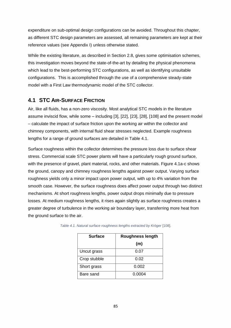
85
expenditure on sub-optimal design configurations can be avoided. Throughout this chapter,
as different STC design parameters are assessed, all remaining parameters are kept at their
reference values (see Appendix I) unless otherwise stated.
While the existing literature, as described in Section 2.8, gives some optimisation schemes,
this investigation moves beyond the state-of-the-art by detailing the physical phenomena
which lead to the best-performing STC configurations, as well as identifying unsuitable
configurations. This is accomplished through the use of a comprehensive steady-state
model with a First Law thermodynamic model of the STC collector.
4.1 STC AIR-SURFACE FRICTION
Air, like all fluids, has a non-zero viscosity. Most analytical STC models in the literature
assume inviscid flow, while some – including [3], [22], [23], [28], [108] and the present model
– calculate the impact of surface friction upon the working air within the collector and
chimney components, with internal fluid shear stresses neglected. Example roughness
lengths for a range of ground surfaces are detailed in Table 4.1.
Surface roughness within the collector determines the pressure loss due to surface shear
stress. Commercial scale STC power plants will have a particularly rough ground surface,
with the presence of gravel, plant material, rocks, and other materials. Figure 4.1a-c shows
the ground, canopy and chimney roughness lengths against power output. Varying surface
roughness yields only a minor impact upon power output, with up to 4% variation from the
smooth case. However, the surface roughness does affect power output through two distinct
mechanisms. At short roughness lengths, power output drops minimally due to pressure
losses. At medium roughness lengths, it rises again slightly as surface roughness creates a
greater degree of turbulence in the working air boundary layer, transferring more heat from
the ground surface to the air.
Table 4.1. Natural surface roughness lengths extracted by Kröger [108].
Surface Roughness length
(m)
Uncut grass 0.07
Crop stubble 0.02
Short grass 0.002
Bare sand 0.0004

86
This behaviour is further demonstrated in Figure 4.1a, where the increasing ground
roughness length can be seen leading to increased heat transfer into the collector working
air and decreased pressure difference through the collector. The increased collector air
temperature change will lead to an increase in power output, while the decrease in collector
air pressure change counteracts this, reducing power output.
Note that Figure 4.1a was generated by simulating the collector only, with a fixed mass flow
rate (5 -1
1.66 10 kgsm , the converged mass flow rate of the reference STC plant). For the
whole STC plant, the collector air temperature rise c
T is a key variable affecting the system
mass flow rate, which is driven by buoyant flow up the chimney. A change in cT as shown
in Figure 4.2 would lead to a change in mass flow rate, and thus in the air velocity over the
collector’s surfaces. This changes the shear stress at the fluid-surface boundary and thus
introduces a secondary effect when changing ground roughness length, clouding this
analysis. For this reason, the effect of increased c
T on m is excluded from Figure 4.1a,
although it cannot be neglected for the plant as a whole (Figure 4.1b includes this effect).
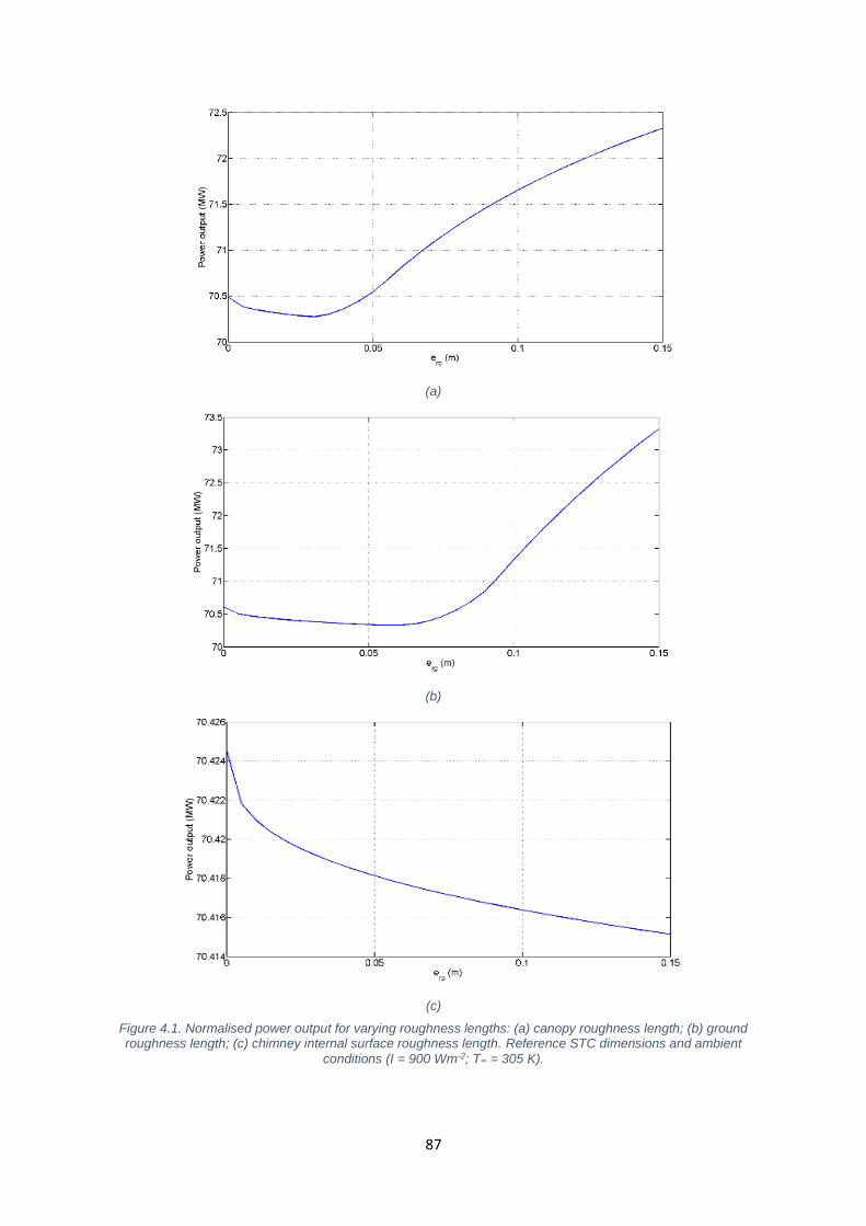
87
(a)
(b)
(c)
Figure 4.1. Normalised power output for varying roughness lengths: (a) canopy roughness length; (b) ground roughness length; (c) chimney internal surface roughness length. Reference STC dimensions and ambient
conditions (I = 900 Wm-2; T∞ = 305 K).
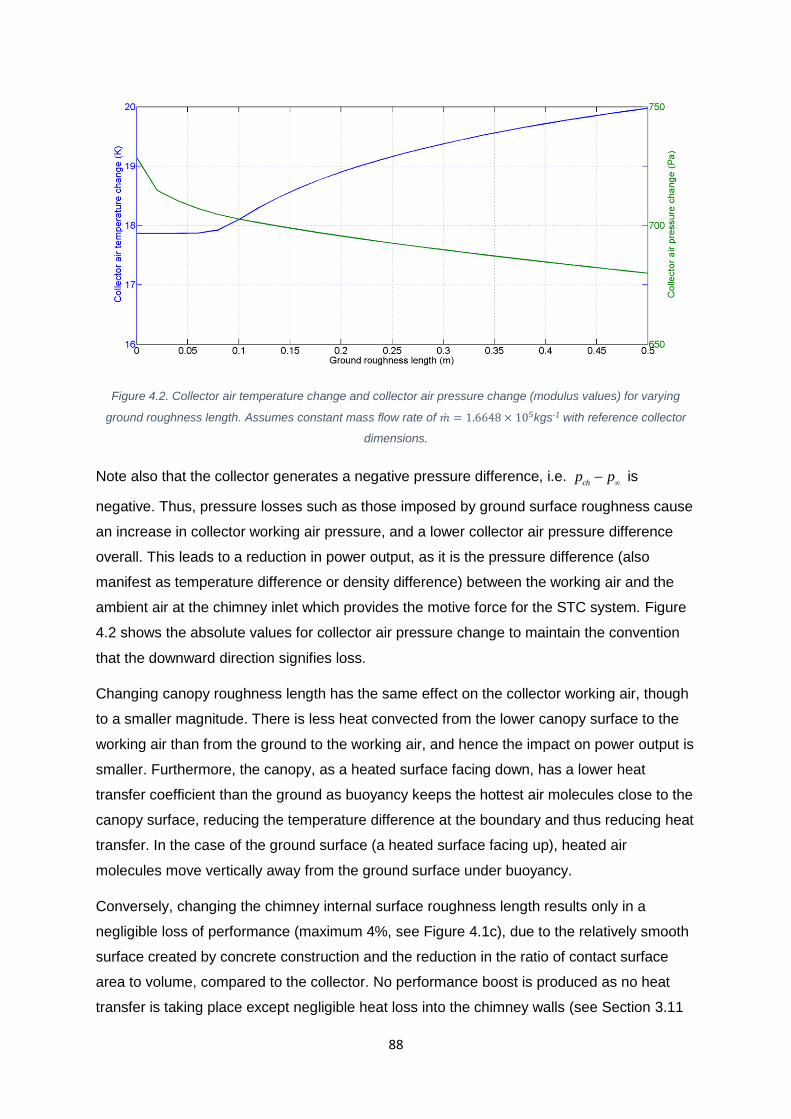
88
Figure 4.2. Collector air temperature change and collector air pressure change (modulus values) for varying
ground roughness length. Assumes constant mass flow rate of �̇� = 1.6648 × 10⁵kgs-1 with reference collector
dimensions.
Note also that the collector generates a negative pressure difference, i.e. ch
p p
is
negative. Thus, pressure losses such as those imposed by ground surface roughness cause
an increase in collector working air pressure, and a lower collector air pressure difference
overall. This leads to a reduction in power output, as it is the pressure difference (also
manifest as temperature difference or density difference) between the working air and the
ambient air at the chimney inlet which provides the motive force for the STC system. Figure
4.2 shows the absolute values for collector air pressure change to maintain the convention
that the downward direction signifies loss.
Changing canopy roughness length has the same effect on the collector working air, though
to a smaller magnitude. There is less heat convected from the lower canopy surface to the
working air than from the ground to the working air, and hence the impact on power output is
smaller. Furthermore, the canopy, as a heated surface facing down, has a lower heat
transfer coefficient than the ground as buoyancy keeps the hottest air molecules close to the
canopy surface, reducing the temperature difference at the boundary and thus reducing heat
transfer. In the case of the ground surface (a heated surface facing up), heated air
molecules move vertically away from the ground surface under buoyancy.
Conversely, changing the chimney internal surface roughness length results only in a
negligible loss of performance (maximum 4%, see Figure 4.1c), due to the relatively smooth
surface created by concrete construction and the reduction in the ratio of contact surface
area to volume, compared to the collector. No performance boost is produced as no heat
transfer is taking place except negligible heat loss into the chimney walls (see Section 3.11

89
for justification). Greater performance losses in the chimney are predicted by Von Backström
et al. [109] due not to the chimney internal surface, but to the internal rim and spokes design
which was proposed by Schlaich [110] to stiffen the tall thin-walled chimney structure (in this
case, 1500 m tall) and provide stability under lateral loads.
4.2 OPTIMUM TURBINE PRESSURE DROP RATIO
The chimney, with its buoyant airflow, makes pressure potential available to the system from
which energy can be generated. The parameter x defines a balance between pressure
potential used to drive flow through the system and pressure potential converted to electrical
energy in the turbines and generators. The greatest system mass flow rate is achieved when
0x , but no energy can then be extracted to generate electricity. Conversely, attempting to
extract all pressure potential energy from the flow ( 1.00x ) will block the flow up the
chimney and reduce the mass flow rate to zero.
The optimum ratio of turbine pressure drop to chimney pressure drop, x , is a subject of
debate in the academic literature (see Chapter 2). The optimum value of x is assessed by
evaluating the performance of the reference STC across a range of values of x . Figure 4.3
shows that the optimum value of x under reference conditions is 0.795. STC performance is
almost flat in the region ..75 50 0 8x , but drops more sharply in the region ..85 00 0 9x .
Figure 4.4 - Figure 4.8 shows the turbine pressure drop ratio’s sensitivity to plant dimensions
and environmental parameters. Figure 4.4 shows that varying insolation causes the optimum
turbine pressure drop ratio to vary across the range ..75 00 0 8x , with optimum values of
x close to 0.80x for medium and high insolation levels.
Figure 4.3. Power output produced by reference STC (Hci = 4.0 m, Hco = 11.5 m) under reference conditions with
a range of turbine pressure drop ratio values.

90
Figure 4.4. STC performance for varying values of turbine pressure drop ratio and insolation.
Figure 4.5. STC performance for varying values of turbine pressure drop ratio and ambient temperature.
Figure 4.6. STC performance for varying values of turbine pressure drop ratio and collector radius.
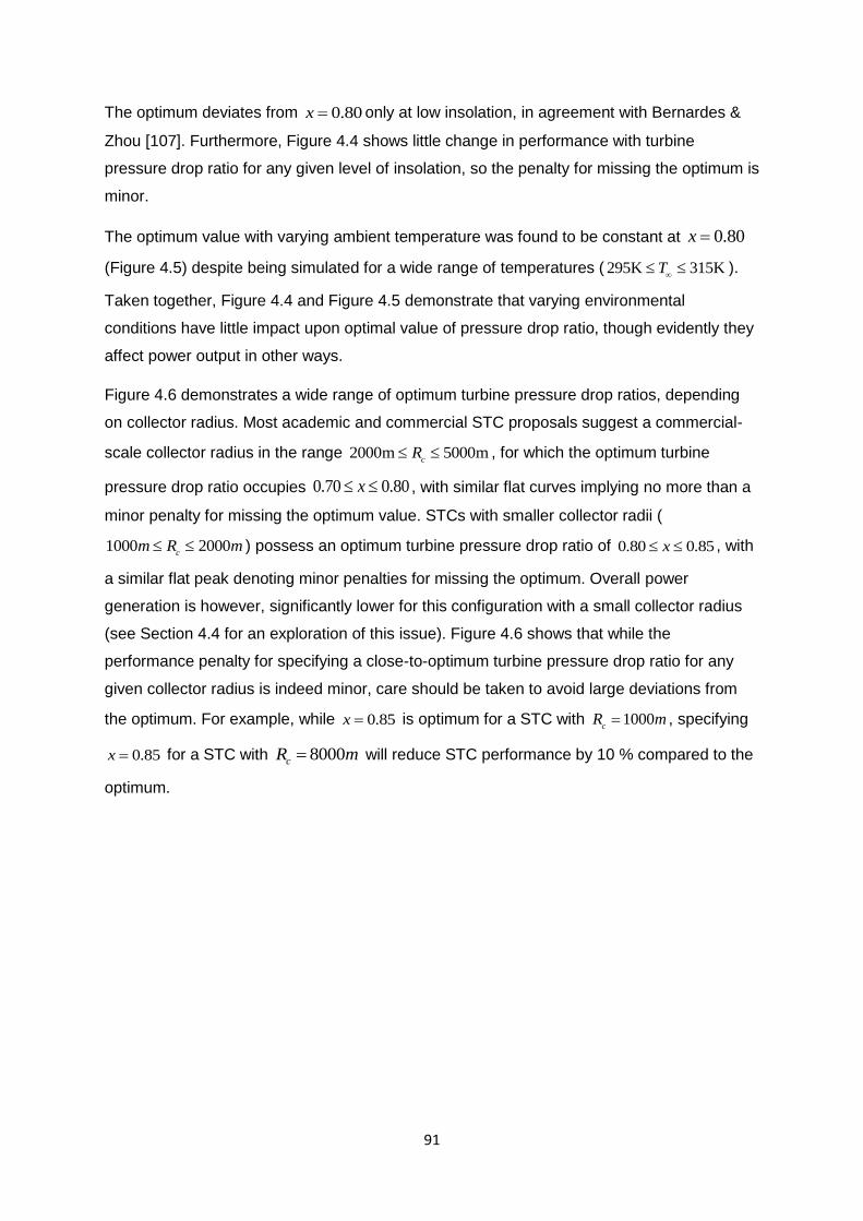
91
The optimum deviates from 0.80x only at low insolation, in agreement with Bernardes &
Zhou [107]. Furthermore, Figure 4.4 shows little change in performance with turbine
pressure drop ratio for any given level of insolation, so the penalty for missing the optimum is
minor.
The optimum value with varying ambient temperature was found to be constant at 0.80x
(Figure 4.5) despite being simulated for a wide range of temperatures ( K 315K295 T
).
Taken together, Figure 4.4 and Figure 4.5 demonstrate that varying environmental
conditions have little impact upon optimal value of pressure drop ratio, though evidently they
affect power output in other ways.
Figure 4.6 demonstrates a wide range of optimum turbine pressure drop ratios, depending
on collector radius. Most academic and commercial STC proposals suggest a commercial-
scale collector radius in the range m 5000m2000c
R , for which the optimum turbine
pressure drop ratio occupies ..70 00 0 8x , with similar flat curves implying no more than a
minor penalty for missing the optimum value. STCs with smaller collector radii (
2000 0001c
R mm ) possess an optimum turbine pressure drop ratio of ..80 50 0 8x , with
a similar flat peak denoting minor penalties for missing the optimum. Overall power
generation is however, significantly lower for this configuration with a small collector radius
(see Section 4.4 for an exploration of this issue). Figure 4.6 shows that while the
performance penalty for specifying a close-to-optimum turbine pressure drop ratio for any
given collector radius is indeed minor, care should be taken to avoid large deviations from
the optimum. For example, while 0.85x is optimum for a STC with 1000c
R m , specifying
0.85x for a STC with 8000cR m will reduce STC performance by 10 % compared to the
optimum.
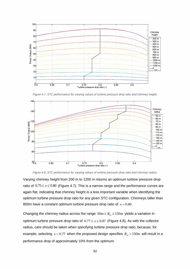
92
Figure 4.7. STC performance for varying values of turbine pressure drop ratio and chimney height.
Figure 4.8. STC performance for varying values of turbine pressure drop ratio and chimney radius.
Varying chimney height from 200 m to 1200 m returns an optimum turbine pressure drop
ratio of ..75 00 0 8x (Figure 4.7). This is a narrow range and the performance curves are
again flat, indicating that chimney height is a less important variable when identifying the
optimum turbine pressure drop ratio for any given STC configuration. Chimneys taller than
800m have a constant optimum turbine pressure drop ratio of 0.80x .
Changing the chimney radius across the range 10m 50m5ch
R yields a variation in
optimum turbine pressure drop ratio of ..77 70 0 8x (Figure 4.8). As with the collector
radius, care should be taken when specifying turbine pressure drop ratio, because, for
example, selecting 0.77x when the proposed design specifies 150ch
R m will result in a
performance drop of approximately 10% from the optimum.
93
In summary, for the selected reference plant dimensions and ambient conditions, the
selected turbine pressure drop value of 0.81x is near optimum. This value of x is kept
constant during the parametric studies presented in this chapter, causing the model to
slightly underestimate peak performance of the configuration under study, as the optimum
value of x moves further from 0.81x . However, Figure 4.4 - Figure 4.8 suggest a tolerant
optimum to variations in the parameters studied, meaning that such an impact is minimised.
The greatest impact can be seen when varying collector radius or chimney radius.
Increasing the collector radius causes the optimum x to fall, from 0.85x for a collector
radius of 1000 m to 0.7x for a collector radius of 5000 m or more. A larger collector radius
can gather more heat from the sun, and hence provide a greater pressure difference in the
chimney (provided the chimney dimensions are large enough – as they are in the reference
STC). Hence a smaller proportion of the available pressure difference is required to drive the
air through the chimney, resulting in a larger pressure difference available to generate
power. The physical mechanism which causes power output to cease rising appreciably with
collector radii beyond 5000mcoll
R is discussed in Section 4.4.
In the case of increasing chimney radius, an increase in x is also required to maintain the
optimum. This is because the chimney internal flow area has increased and therefore a
greater mass of air must now be moved up through the chimney to maintain flow through the
STC. A greater pressure difference is required to maintain this flow. The collector size
remains the same, so the solar input does not change. The total buoyant pressure difference
changes only slightly, due to a change in the flow velocity through the collector, which
changes the heat transfer coefficients between the working air flow and the collector’s
internal surfaces. Hence, in order to meet the larger pressure difference required to drive the
airflow up the chimney, a greater proportion of the available buoyancy pressure difference
must be given over to generating airflow, with a reduced proportion available to generate
power. Note that increasing collector radius increases the total volume flow rate through the
system, and hence it increases power output regardless of the change in optimum x .
Bernardes & Zhou [107] used a comprehensive STC model to establish optimum turbine
pressure drop ratios for varying insolation. The authors ran simulations for sets of insolation
scenarios representing likely daily weather patterns (e.g. sun followed by cloud cover). They
established that optimum turbine pressure drop ratios deviated little from 0.80x ,
regardless of insolation level. Only when the insolation fell to zero (e.g. at night) did they find
that optimum turbine pressure drop ratio fell rapidly, tending towards zero. As previously
discussed, a value of 0x implies a turbine configuration unable to extract any useful
power from the buoyant updraft. The analysis presented herein is in broad agreement with
94
Bernardes & Zhou regarding optimum turbine pressure drop ratio compared to varying
insolation. Figure 4.4 shows the optimum turbine pressure drop ratio to be stable at 0.80x
for all except the lowest insolation values, for which the optimum ratio drops slightly.
Following Bernardes & Zhou, it is expected that the optimum ratio would drop further for
even lower insolation values.
4.3 STC SENSITIVITY ANALYSIS
The model presented in Chapter 3 permits us to investigate how STC performance changes
as plant parameters are varied. As expected, a change in insolation brings about a linearly
proportional change in power output (Figure 4.10a), with slight non-linearities present due to
changes in collector efficiency. Insolation affects collector efficiency by altering the air
temperature rise through the collector, thereby changing the buoyancy pressure difference in
the chimney and thus changing the working air velocity profile through the collector. Heat
transfer from the heated ground and canopy surfaces to the working air is heavily dependent
upon the velocity of the working air, and an increase in air velocity correspondingly increases
collector efficiency.
High-insolation areas are best-suited to deliver high power output from STCs. However,
such environments (e.g. deserts) are normally also characterised by high ambient air
temperatures (at least during the daytime). Figure 4.10b shows that increasing ambient air
temperature reduces STC power output. This is caused by two factors. Firstly, radiative heat
is lost to the environment at a rate proportional to the difference between the fourth power of
the canopy surface temperature and the fourth power of the theoretical clear sky
temperature, as outlined in Chapter 3. If an assumption is made that the difference between
the collector canopy temperature and the ambient air temperature remains constant, an
increase in ambient air temperature results in a roughly linear increase in energy radiated
from the canopy of 1.8 W per Kelvin of ambient temperature increase per square metre of
the canopy, as shown in Figure 4.9.
Secondly, less energy is required to decrease the density of a flowing fluid already at a
higher temperature, compared to the same fluid at a lower temperature, as is evident in the
model’s Boussinesq approximation for the gas equation of state:
T T
T
(4.1)
Achieving a density change from -3
1.00kgm to
-30.95kgm at an ambient
temperature of 305KT requires a temperature difference of 15.25KT . Other

95
temperature differences required to achieve the same density difference from different initial
ambient temperatures are shown in Table 4.2. The range of temperature differences
required is narrow, suggesting that this mechanism is responsible for a smaller proportion of
the power drop due to increasing ambient temperature than the issue of radiative heat loss
outlined above.
The impact of ambient wind velocity on the thermodynamic performance of the STC is an
important issue in need of consideration. In the current model, heat losses due to ambient
wind velocity above the collector canopy upper surface are included. It is assumed that the
atmosphere is an infinitely large heat sink and that consequently the ambient air temperature
does not change. Convective heat loss due to ambient wind velocity proves to have a
serious impact on STC performance (Figure 4.10c). This, and the issue of ambient wind
causing convective heat loss beneath the collector canopy, have been identified by various
authors (Ming et al. [57] & Zhou et al. [56]), who have proposed a range of solutions to limit
its impact, as detailed in Chapter 6. Without heat loss mitigation built into the collector
design, even low ambient wind velocities cause significant reductions in power output. In the
case of the reference STC plant under reference conditions, it experienced a power loss of
18 % when the ambient wind velocity increased from 0 ms-1 to 2 ms-1. Further increases in
wind velocity see the power output drop by 50 %, from 70 MW (10wv ms ) to 35 MW (
115
wv ms
).
Figure 4.9. Rate of heat flux radiated from canopy surface to the sky for changing ambient air temperature.
Assumes a constant temperature difference between ambient air and canopy surface.
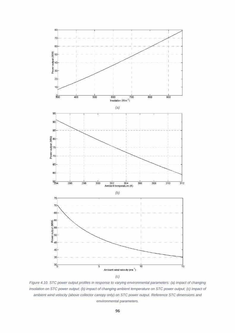
96
(a)
(b)
(c)
Figure 4.10. STC power output profiles in response to varying environmental parameters: (a) impact of changing
insolation on STC power output; (b) impact of changing ambient temperature on STC power output; (c) impact of
ambient wind velocity (above collector canopy only) on STC power output. Reference STC dimensions and
environmental parameters.
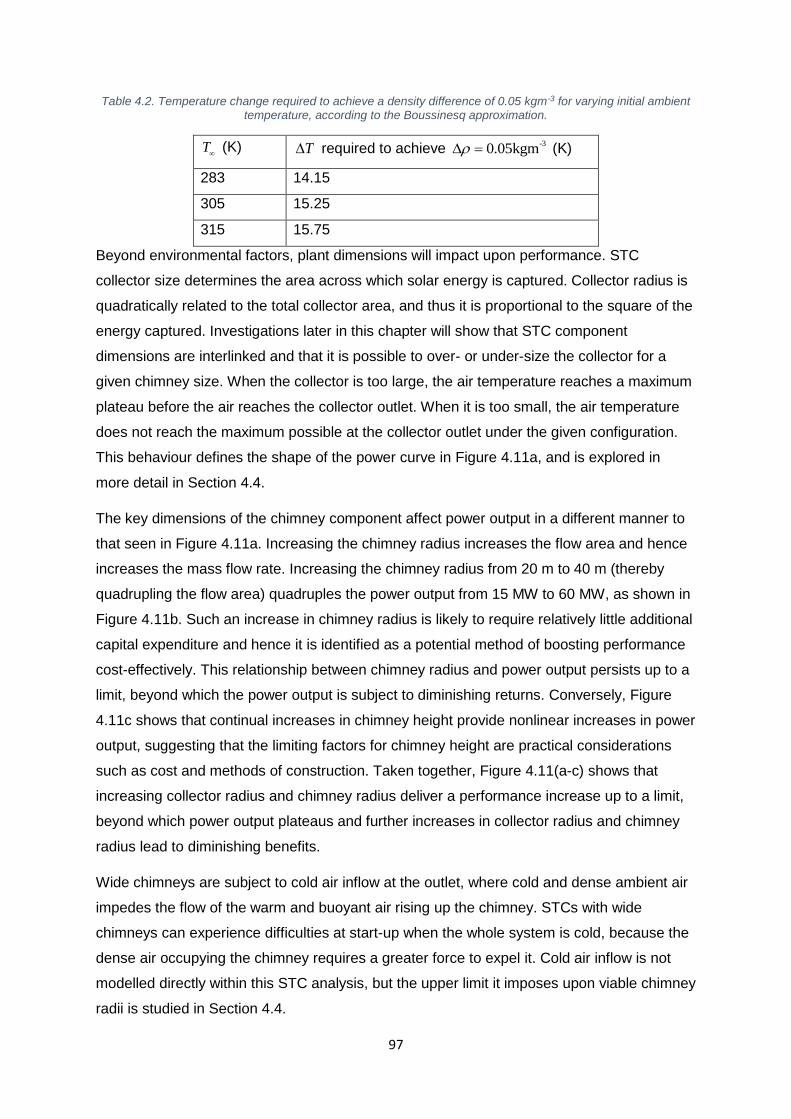
97
Table 4.2. Temperature change required to achieve a density difference of 0.05 kgm-3 for varying initial ambient temperature, according to the Boussinesq approximation.
T
(K) T required to achieve -3
0.05kgm (K)
283 14.15
305 15.25
315 15.75
Beyond environmental factors, plant dimensions will impact upon performance. STC
collector size determines the area across which solar energy is captured. Collector radius is
quadratically related to the total collector area, and thus it is proportional to the square of the
energy captured. Investigations later in this chapter will show that STC component
dimensions are interlinked and that it is possible to over- or under-size the collector for a
given chimney size. When the collector is too large, the air temperature reaches a maximum
plateau before the air reaches the collector outlet. When it is too small, the air temperature
does not reach the maximum possible at the collector outlet under the given configuration.
This behaviour defines the shape of the power curve in Figure 4.11a, and is explored in
more detail in Section 4.4.
The key dimensions of the chimney component affect power output in a different manner to
that seen in Figure 4.11a. Increasing the chimney radius increases the flow area and hence
increases the mass flow rate. Increasing the chimney radius from 20 m to 40 m (thereby
quadrupling the flow area) quadruples the power output from 15 MW to 60 MW, as shown in
Figure 4.11b. Such an increase in chimney radius is likely to require relatively little additional
capital expenditure and hence it is identified as a potential method of boosting performance
cost-effectively. This relationship between chimney radius and power output persists up to a
limit, beyond which the power output is subject to diminishing returns. Conversely, Figure
4.11c shows that continual increases in chimney height provide nonlinear increases in power
output, suggesting that the limiting factors for chimney height are practical considerations
such as cost and methods of construction. Taken together, Figure 4.11(a-c) shows that
increasing collector radius and chimney radius deliver a performance increase up to a limit,
beyond which power output plateaus and further increases in collector radius and chimney
radius lead to diminishing benefits.
Wide chimneys are subject to cold air inflow at the outlet, where cold and dense ambient air
impedes the flow of the warm and buoyant air rising up the chimney. STCs with wide
chimneys can experience difficulties at start-up when the whole system is cold, because the
dense air occupying the chimney requires a greater force to expel it. Cold air inflow is not
modelled directly within this STC analysis, but the upper limit it imposes upon viable chimney
radii is studied in Section 4.4.
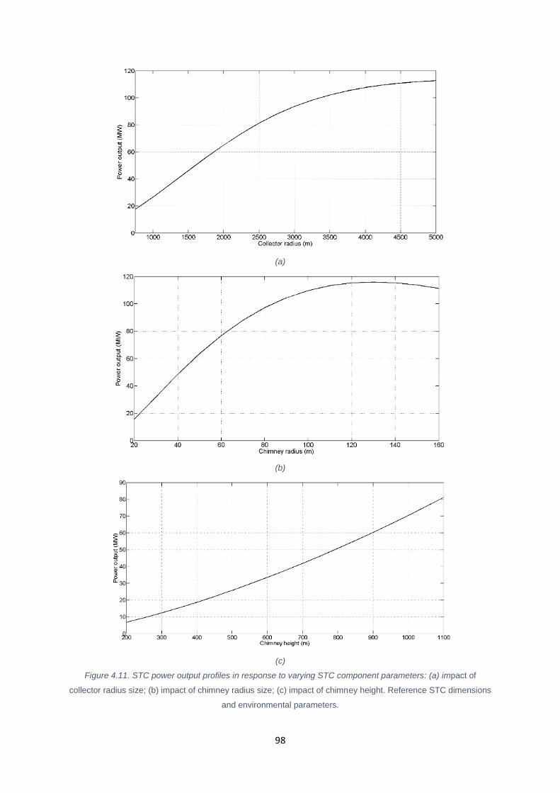
98
(a)
(b)
(c)
Figure 4.11. STC power output profiles in response to varying STC component parameters: (a) impact of
collector radius size; (b) impact of chimney radius size; (c) impact of chimney height. Reference STC dimensions
and environmental parameters.
99
4.4 DIMENSION MATCHING
Several authors have carried out parametric studies and identified optimum dimensions,
both in terms of cost and in terms of the best-performing dimensions of a component when
all other components’ dimensions are fixed (e.g. changing collector radius only). Koonsrisuk
& Chitsomboon [98] assessed sloping canopies and flaring chimneys (diverging chimney
walls), and concluded that significant boosts to power output could be obtained with these
design modifications. Dehghani & Mohammadi [73] used an optimisation scheme to find the
best-performing STC dimensions using a simple STC thermodynamic model that didn’t
include full thermodynamic simulation of the collector thermal network. They found a set of
pareto-optimal configurations, in which the chimney height optimised at the upper limit of the
study. Dehghani & Mohammadi performed further analysis on five STC configurations
selected at random from the Pareto-optimal set. The present work will build upon the work of
Dehghani & Mohammadi by employing a comprehensive STC model with dynamic heat
transfer modelling, permitting greater analysis of the technical mechanisms behind the
optimal dimensions.
Gholamalizadeh & Kim [72] present a similar analysis, wherein a set of pareto-optimal STC
configurations are identified by means of a multi-objective optimisation algorithm. Similarly to
Dehghani & Mohammadi, Gholamalizadeh & Kim utilise a simple STC model which does not
permit in-depth analysis of the technical mechanisms which determine optimal dimensions.
Rather, Gholamalizadeh & Kim establish the plant efficiency and calculate the STC power
output as the product of system efficiency and solar radiation incident upon the collector.
Both Dehghani & Mohammadi and Gholamalizadeh & Kim make use of simple cost models
in which STC cost is assumed to be proportional to the individual components’ surface area
(e.g. collector cost is proportional to collector surface area).
This study will build upon these existing works by investigating “matching” sets of STC
dimensions, in which no component is over-sized (too much expenditure) or under-sized (too
little return on expenditure), and in particular investigating the physical processes that affect
the working air within the STC to produce the best-performing STC configuration.
Parametric studies undertaken in this investigation have varied the key dimensions of STC
components within a given range. Increasing the chimney height increases both system
efficiency and mass flow rate (Zhou et al. [37]). Whilst the engineering design and
construction of very tall chimneys remains a significant challenge, a large body of STC
technical literature has considered STC plants with a chimney height in the region of 1000m
(e.g. Fluri et al. [4], Bernardes et al. [3], & Pretorius et al. [16]). Optimisation studies
available in the literature show that STC design configurations always optimise with the

100
chimney height at the upper bound of the study. As different technical and economic
limitations will exist for different projects around the world, this study has taken a different
approach. This study considers three chimney heights in the range m 1000m500ch
H , and
identifies different sets of best-performing (“matched”) dimensions for each chimney height.
For the purposes of this study, the collector canopy profile has been assumed to be linearly
sloped, rising from 4 m at the collector inlet to 24 m at the collector outlet. This has been
found to be the best-performing collector outlet height for an STC with collector radius of
5500 m, chimney height of 1000 m, and chimney radius of 55 m (Figure 4.12). Figure 4.12
shows that the power output increases substantially for wider chimneys, and that wider
chimneys require different canopy outlet heights to achieve optimum performance. Narrow
chimneys ( 20 100ch
mm R ) require a canopy outlet height of 24 m or less, and canopy
outlet heights other than the optimum do not incur significant performance penalties. Wider
chimneys (100 200ch
m R m ) require progressively taller canopies at the collector outlet, up
to 40 m tall for 200ch
R m . The detrimental effect upon performance of missing the optimum
outlet canopy height also increases. For example, specifying a canopy outlet height of 24 m
for a STC with a chimney radius of 200 m results in a loss of approximately 10 % of power
output, compared to the best-performing configuration. The greatest loss of performance
occurs for STCs with large chimney radii (100 200ch
m R m ), but smaller-than-optimum
canopy outlet heights. Specifying taller-than-optimum canopy outlet heights imposes less of
a performance penalty, but is inadvisable as it represents additional expenditure without
commensurate performance benefits.
Figure 4.12. Power output for STCs with varying collector canopy outlet height and chimney radius. Rc = 5500 m,
Hch = 1000 m, Hci = 4 m, I = 900 Wm-2, T∞ = 305 K.

101
Under-sizing any one of these parameters can limit power output in the following ways:
1. The collector and chimney should be sized such that the airflow reaches thermal
equilibrium with the other collector components only at the collector outlet. If the
collector radius is too small, too little heat is captured from sun and the air is not heated
to thermal equilibrium. Hence, for the given chimney dimensions, more energy could be
absorbed into the airflow if the STC possessed a larger collector.
2. The working airflow is too slow, therefore insufficient heat is transferred from collector
surfaces (i.e. collector canopy not the right shape for high-velocity flow). This is due to
the dependence of the convective heat transfer coefficients upon air velocity, and is
caused by an under-sized chimney for a given collector.
Figure 4.13a-c shows the dependency of power output on collector radius and chimney
radius for three chimney heights, and demonstrates that for any given STC configuration
there exists a collector radius beyond which no performance increases can be gained by
increasing the collector size. This is due to the collector thermal components – the ground,
the working air, and the canopy – approaching thermal equilibrium, resulting in negligible
further net heat transfer to the working air. Figure 4.13a-c also highlights large power boosts
available from very large-scale STC power plants. Up to 690 MW can be generated by the
largest plant in the study (Rc = 7000 m, Hco = 24 m, Rch = 200 m, Hch = 1000 m). This is
mainly due to the massively increased chimney radius, which permits the chimney to
produce a far greater mass flow rate for the same pressure difference, i.e. for the same
temperature rise generated by the collector. Large-radius chimneys risk suffering from cold
air inflow at the chimney outlet, which may reduce the maximum achievable power output.
This is discussed later in this chapter.
Collector thermal equilibrium is apparent in configurations with smaller chimney radii and
larger collector radii, regardless of chimney height. For example, Figure 4.13a shows that for
a chimney 500 m tall with an internal flow radius of 60m, a collector with a radius of 5.0 km
generates the same power output as a collector of radius 7.0 km. This means that increasing
collector radius from 5.0 km to 7.0 km – thereby doubling the collector area – is non-
productive, and the smaller collector size can be selected without reducing the STC’s power
output.
The plateau in STC performance despite larger collector radii can be overcome by
increasing chimney height and chimney radius. Figure 4.13a shows that a STC with a
chimney height of 500 m and a chimney radius of 60 m has a peak power output of
approximately 45 MW, regardless of collector size. Figure 4.13c shows that a STC with a
chimney of the same radius but double the height (1000 m) has a peak power output of 140
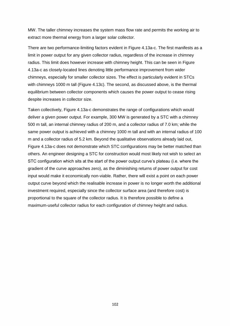
102
MW. The taller chimney increases the system mass flow rate and permits the working air to
extract more thermal energy from a larger solar collector.
There are two performance-limiting factors evident in Figure 4.13a-c. The first manifests as a
limit in power output for any given collector radius, regardless of the increase in chimney
radius. This limit does however increase with chimney height. This can be seen in Figure
4.13a-c as closely-located lines denoting little performance improvement from wider
chimneys, especially for smaller collector sizes. The effect is particularly evident in STCs
with chimneys 1000 m tall (Figure 4.13c). The second, as discussed above, is the thermal
equilibrium between collector components which causes the power output to cease rising
despite increases in collector size.
Taken collectively, Figure 4.13a-c demonstrates the range of configurations which would
deliver a given power output. For example, 300 MW is generated by a STC with a chimney
500 m tall, an internal chimney radius of 200 m, and a collector radius of 7.0 km; while the
same power output is achieved with a chimney 1000 m tall and with an internal radius of 100
m and a collector radius of 5.2 km. Beyond the qualitative observations already laid out,
Figure 4.13a-c does not demonstrate which STC configurations may be better matched than
others. An engineer designing a STC for construction would most likely not wish to select an
STC configuration which sits at the start of the power output curve’s plateau (i.e. where the
gradient of the curve approaches zero), as the diminishing returns of power output for cost
input would make it economically non-viable. Rather, there will exist a point on each power
output curve beyond which the realisable increase in power is no longer worth the additional
investment required, especially since the collector surface area (and therefore cost) is
proportional to the square of the collector radius. It is therefore possible to define a
maximum-useful collector radius for each configuration of chimney height and radius.

103
Figure 4.13. STC power output for varying combinations of chimney radius and collector radius. Hci = 4 m; Hco =
24 m; I = 900 Wm-2; T∞ = 305 K.
Figure 4.14 shows the thermal component temperature profiles along the radial path for
three different collector sizes. The air enters the collector at ambient temperature (right hand
side of the figure) and flows towards the collector centre (left hand side of the figure), where
it exits to the turbines and chimney. The air temperatures, represented by solid lines, reach a
maximum plateaued value for the two larger collectors (Rc = 3.25 km; Rc = 4.50 km), a limit
enforced by thermal equilibrium of the collector components. The reduction in temperatures
close to the collector outlet (right hand side of the figure) is due to rapid increases in air
velocity as the flow area constricts. Thus we can theorise that the ideally-sized collector
would be one in which the thermal components reach their equilibrium temperatures at the
collector outlet, thus ensuring that maximum thermal energy has been transferred to the
airflow without over-sizing the collector in order to do so. After air temperature plateaus, any
continued change in ground or canopy temperatures is effected via radiative heat transfer,
which the model assumes does not contribute to air temperature change (in agreement with
Bernardes et al. [3] and Pretorius et al. [16]). A STC with fully-matched dimensions would
see the thermal components approach thermal equilibrium just at the collector outlet
(dependent upon ambient conditions).
It should be noted that the model has produced some small oscillations of ground
temperatures close to the collector outlet, observable in Figure 4.14 for the largest collector
radius.
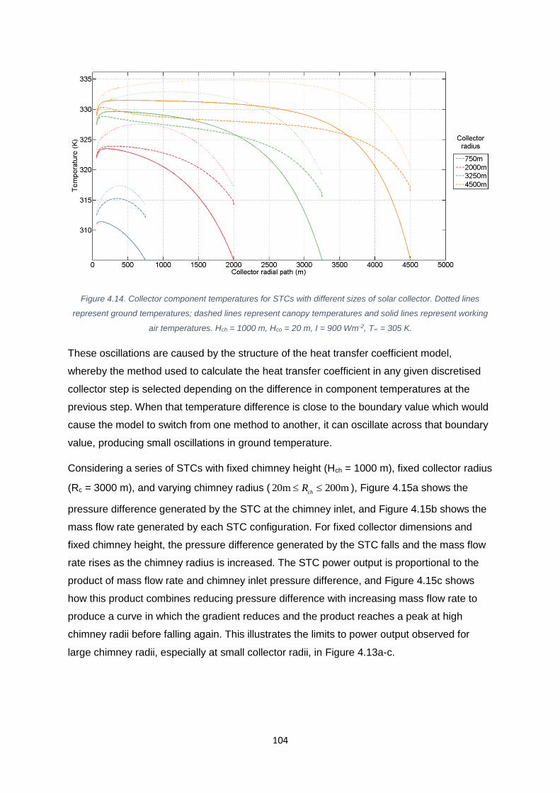
104
Figure 4.14. Collector component temperatures for STCs with different sizes of solar collector. Dotted lines
represent ground temperatures; dashed lines represent canopy temperatures and solid lines represent working
air temperatures. Hch = 1000 m, Hco = 20 m, I = 900 Wm-2, T∞ = 305 K.
These oscillations are caused by the structure of the heat transfer coefficient model,
whereby the method used to calculate the heat transfer coefficient in any given discretised
collector step is selected depending on the difference in component temperatures at the
previous step. When that temperature difference is close to the boundary value which would
cause the model to switch from one method to another, it can oscillate across that boundary
value, producing small oscillations in ground temperature.
Considering a series of STCs with fixed chimney height (Hch = 1000 m), fixed collector radius
(Rc = 3000 m), and varying chimney radius ( 20m 00m2ch
R ), Figure 4.15a shows the
pressure difference generated by the STC at the chimney inlet, and Figure 4.15b shows the
mass flow rate generated by each STC configuration. For fixed collector dimensions and
fixed chimney height, the pressure difference generated by the STC falls and the mass flow
rate rises as the chimney radius is increased. The STC power output is proportional to the
product of mass flow rate and chimney inlet pressure difference, and Figure 4.15c shows
how this product combines reducing pressure difference with increasing mass flow rate to
produce a curve in which the gradient reduces and the product reaches a peak at high
chimney radii before falling again. This illustrates the limits to power output observed for
large chimney radii, especially at small collector radii, in Figure 4.13a-c.

105
Figure 4.15. Effect of chimney radius on flow parameters: (a) Chimney inlet pressure potential; (b) system mass
flow rate; (c) product of pressure potential and mass flow rate. Rc = 3000 m; Hch = 1000 m; Hci = 4 m; Hco = 16 m;
I = 900 Wm-2; T∞ = 305 K.
By interrogating Figure 4.13a-c, one can observe that the gradient of the power output curve
decreases before approaching the plateau. STC performance can therefore be characterised
in terms of power gradient, that is: change in power output with respect to change in
collector surface area. The collector surface area was chosen to eliminate the quadratic
behaviour inherent in the relationship between power and collector radius. As the power
output curve approaches its plateau, the gradient curve will approach zero.
Figure 4.16a-c shows the gradient of the power output for varying chimney height, chimney
radius and collector surface area. The power output plateaus can be seen particularly in
Figure 4.16c, as the gradient values approach zero. An engineer tasked with designing a
STC for construction can make use of Figure 4.16a-c: By setting a minimum limiting value
for the gradient d / dc
P A , he or she can eliminate STC design configurations for which further
increases in component dimensions do not yield sufficient returns in terms of power output.
All STC configurations which deliver a value for d / dc
P A below the minimum specified by the
engineer (dependent upon cost constraints of the specific project) can be disregarded as
economically non-viable.
While the existence of non-viable STC configurations has been established, further work is
required to identify optimal dimensions for given constraints. As multiple different
configurations will return the same power output, a further constraint is required to identify
optimal configurations.
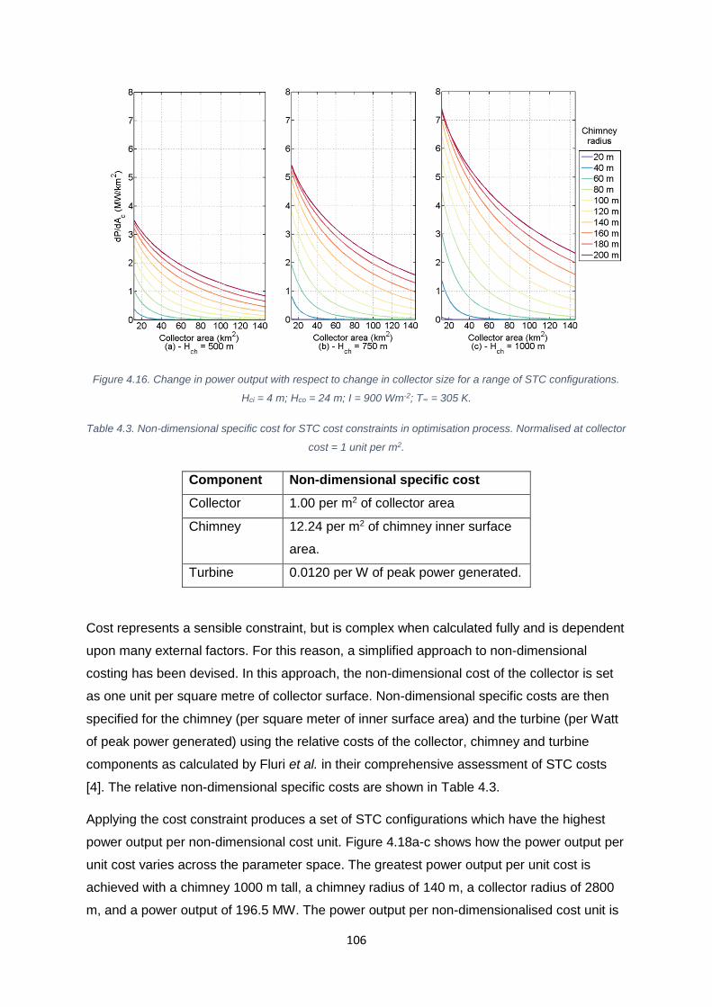
106
Figure 4.16. Change in power output with respect to change in collector size for a range of STC configurations.
Hci = 4 m; Hco = 24 m; I = 900 Wm-2; T∞ = 305 K.
Table 4.3. Non-dimensional specific cost for STC cost constraints in optimisation process. Normalised at collector
cost = 1 unit per m2.
Component Non-dimensional specific cost
Collector 1.00 per m2 of collector area
Chimney 12.24 per m2 of chimney inner surface
area.
Turbine 0.0120 per W of peak power generated.
Cost represents a sensible constraint, but is complex when calculated fully and is dependent
upon many external factors. For this reason, a simplified approach to non-dimensional
costing has been devised. In this approach, the non-dimensional cost of the collector is set
as one unit per square metre of collector surface. Non-dimensional specific costs are then
specified for the chimney (per square meter of inner surface area) and the turbine (per Watt
of peak power generated) using the relative costs of the collector, chimney and turbine
components as calculated by Fluri et al. in their comprehensive assessment of STC costs
[4]. The relative non-dimensional specific costs are shown in Table 4.3.
Applying the cost constraint produces a set of STC configurations which have the highest
power output per non-dimensional cost unit. Figure 4.18a-c shows how the power output per
unit cost varies across the parameter space. The greatest power output per unit cost is
achieved with a chimney 1000 m tall, a chimney radius of 140 m, a collector radius of 2800
m, and a power output of 196.5 MW. The power output per non-dimensionalised cost unit is

107
5.21 W/unit. Given that the non-dimensionalised cost unit is specified as one unit per square
metre of collector area, this data also reveals that this STC configuration generates 5.21 W
(peak) per square metre of collector area.
As identified above, the cost units are arbitrary and it is the ratio of costs of different
components which is of importance. In order to assess the sensitivity of the optimum to
these cost ratios, a brief sensitivity analysis was conducted, in which the costs of the
chimney and turbine were halved relative to the collector (scenario 2) and doubled relative to
the collector (scenario 3). The results are given in Table 4.4. Halving the cost of the chimney
and turbine relative to the collector had little effect on optimal dimensions, and it increased
the power generated per unit spent, as would be expected. Doubling the cost of the chimney
and turbine led to a larger chimney (160 m radius as opposed to 140 m) and a significantly
larger collector (4000 m radius – 204 % of the size of the scenario 1 optimum collector). This
leads inevitably to lower power output per unit spent. However, Figure 4.17 shows that a
range of configurations would deliver a very similar performance close to the optimum,
including a STC with a 1000m-tall chimney, 140 m chimney radius, 3600 m collector radius,
and a specific power output of 4.03 W/unit. While this configuration is no more cost-effective
than the optimum, it is smaller and therefore may be more suitable for some projects.
Figure 4.18a-c shows that exceptionally large collectors (with an area greater than 100 km2)
are economically sub-optimal unless the chimney flow area is commensurably increased.
Similarly, increasing chimney height yields an improvement in performance for all
configurations except those with a combination of exceptionally large collector area and
small chimney flow area.
Figure 4.17. Power output per unit cost for Scenario 3 costs (wherein the chimney and turbine have double the
relative cost compared to the collector than that specified by Fluri et al.)
108
Table 4.4. Sensitivity analysis of optimal dimensions for different ratios of component unit costs. All costs are
given relative to the collector, which has a specific cost of 1 unit/m2 of collector area.
Relative
chimney
cost
(units)
Relative
turbine
cost
(units)
Optimum
chH (m)
Optimum
chR (m)
Optimum
cR (m)
Specific
power
output
(W/unit)
Scenario 1 (from
Fluri et al.) 12.24 0.0120 1000 140 2800 5.21
Scenario 2
(chimney and
turbine are half the
relative cost
specified in
scenario 1)
6.12 0.006 1000 140 3000 6.45
Scenario 3
(chimney and
turbine are twice
the relative cost
specified in
scenario 1)
24.48 0.0240 1000 160 4000 4.04
Figure 4.18a-c shows that the most economical STC configuration does not require the
largest chimney diameter, nor the largest collector. This suggests that multiple smaller STCs
may be required to achieve the lowest cost per unit of energy produced. Note, however, that
“small” is relative, as the cost-optimal STC configurations identified here remain extremely
large compared to even the largest modern constructions. The 1000 m tall chimney is shown
to be essential in achieving the greatest possible power output per unit cost. The simple cost
model used in this analysis - wherein the chimney cost is proportional to its internal surface
area - may prove to be insufficient for chimney costing, as the risks and technical challenges
increase with increasing chimney height. Hence the present model may underestimate
chimney costs and exaggerate the power-per-unit-cost benefits of building taller chimneys.
Very large chimney structures with a large flow area are susceptible to a phenomenon called
cold air inflow, which also afflicts cooling towers. The STC relies upon the flow of buoyant air
through the collector, chimney and turbines to generate power. The chimney outlet is found
at height, where the ambient air is colder and therefore denser than the updraft of buoyant
working air. The cold ambient air at the chimney outlet can impede the flow of the working air
and reduce the pressure difference from which power is generated. The cold ambient air can
also flow into the chimney and counter the flow of the updraft, reducing the available
pressure difference still further.
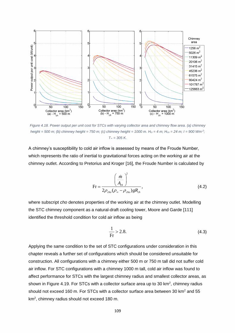
109
Figure 4.18. Power output per unit cost for STCs with varying collector area and chimney flow area. (a) chimney
height = 500 m; (b) chimney height = 750 m; (c) chimney height = 1000 m. Hci = 4 m; Hco = 24 m; I = 900 Wm-2;
T∞ = 305 K.
A chimney’s susceptibility to cold air inflow is assessed by means of the Froude Number,
which represents the ratio of inertial to gravitational forces acting on the working air at the
chimney outlet. According to Pretorius and Kroger [16], the Froude Number is calculated by
2
(Fr ,
2 )
ch
cho cho ch
m
A
gR
(4.2)
where subscript cho denotes properties of the working air at the chimney outlet. Modelling
the STC chimney component as a natural-draft cooling tower, Moore and Garde [111]
identified the threshold condition for cold air inflow as being
1
Fr2.8. (4.3)
Applying the same condition to the set of STC configurations under consideration in this
chapter reveals a further set of configurations which should be considered unsuitable for
construction. All configurations with a chimney either 500 m or 750 m tall did not suffer cold
air inflow. For STC configurations with a chimney 1000 m tall, cold air inflow was found to
affect performance for STCs with the largest chimney radius and smallest collector areas, as
shown in Figure 4.19. For STCs with a collector surface area up to 30 km2, chimney radius
should not exceed 160 m. For STCs with a collector surface area between 30 km2 and 55
km2, chimney radius should not exceed 180 m.
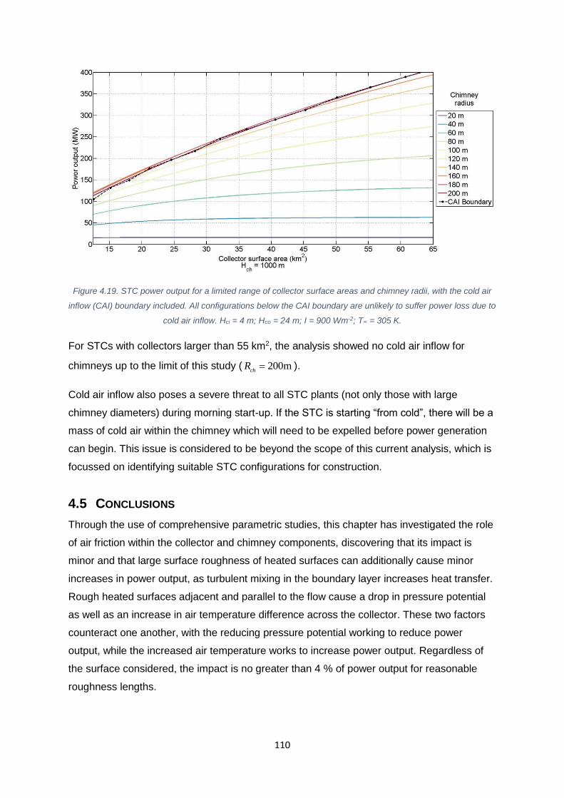
110
Figure 4.19. STC power output for a limited range of collector surface areas and chimney radii, with the cold air
inflow (CAI) boundary included. All configurations below the CAI boundary are unlikely to suffer power loss due to
cold air inflow. Hci = 4 m; Hco = 24 m; I = 900 Wm-2; T∞ = 305 K.
For STCs with collectors larger than 55 km2, the analysis showed no cold air inflow for
chimneys up to the limit of this study ( 200mch
R ).
Cold air inflow also poses a severe threat to all STC plants (not only those with large
chimney diameters) during morning start-up. If the STC is starting “from cold”, there will be a
mass of cold air within the chimney which will need to be expelled before power generation
can begin. This issue is considered to be beyond the scope of this current analysis, which is
focussed on identifying suitable STC configurations for construction.
4.5 CONCLUSIONS
Through the use of comprehensive parametric studies, this chapter has investigated the role
of air friction within the collector and chimney components, discovering that its impact is
minor and that large surface roughness of heated surfaces can additionally cause minor
increases in power output, as turbulent mixing in the boundary layer increases heat transfer.
Rough heated surfaces adjacent and parallel to the flow cause a drop in pressure potential
as well as an increase in air temperature difference across the collector. These two factors
counteract one another, with the reducing pressure potential working to reduce power
output, while the increased air temperature works to increase power output. Regardless of
the surface considered, the impact is no greater than 4 % of power output for reasonable
roughness lengths.

111
This chapter has also investigated the role of turbine to chimney pressure drop ratio in
determining power output. In line with existing literature, the optimum ratio was found to be
0.8x , and remain constant for varying ambient temperature and for higher insolation
levels. Bernardes & Zhou [107] investigated STC performance and the change in turbine
pressure drop ratio under varying insolation and came to the same conclusion. This study
further compliments the work of Bernardes & Zhou by confirming that the optimum pressure
drop ratio is not sensitive to changes in ambient temperature. However, it was discovered
that the optimum pressure drop ratio changes significantly with collector radius and chimney
radius (with all other STC parameters fixed at reference values).
This chapter has sought to uncover the means by which future STC researchers and
engineers can rapidly decide upon suitable plant dimensions. Having noted that continually
increasing collector radius does not produce a commensurate continual increase in power
output, a series of STCs were simulated with varying chimney height, chimney radius and
collector radius. It was discovered that power output ceases to increase for large collector
radii because the airflow within the collector ceases to increase in temperature once the
collector’s thermal components enter thermal equilibrium (i.e. no net heat is transferred
between them). Thus, for given chimney dimensions, it is possible to over-size the collector.
Conversely, a small collector radius may not permit the airflow to reach its greatest possible
temperature difference (defined by the thermal equilibrium), and thus such a collector is
undersized.
As collector radius is increased, the power output is subject to diminishing returns, prior to
reaching a plateau at collector thermal equilibrium. Furthermore, due to a collector’s circular
geometry, the covered area (and thus the cost) is proportional to the square of the radius.
Taken together, these facts strongly suggest that a collector designed such that its thermal
components enter equilibrium just as the air exits the collector at its centre is unlikely to be
economically viable. The analyses carried out in this chapter have led to the identification of
a specific configuration of STC dimensions which will deliver the greatest power output per
unit cost (Hch = 1000 m, Rch = 140 m, Rc = 2800 m, power output per unit cost = 5.21 W/unit).
Figure 4.19 above shows that this configuration is at risk of experiencing cold air inflow at
the chimney outlet. The process of identifying the best-performing configuration is dependent
upon the relative costs assigned to the different STC components. Once these relative costs
are established, this method can be used by future researchers to simplify the process of
selecting the best-performing STC configuration. Analysis of conditions at the chimney outlet
has identified some configurations with particularly large chimneys as being subject to cold
air inflow, resulting in power losses – which in this analysis remain unquantified. These
configurations should be avoided and hence the best-performing configuration with greatest
112
power output per unit relative cost not subject to cold air inflow has been identified. Future
engineers designing commercial-scale STCs will additionally have to consider material
choices, including ground material; selection of low-temperature heat storage materials; and
collector materials.
Further work should include a full cost analysis to improve the accuracy of cost projections,
as well as improve the accuracy of the process of selecting best-performing STC component
dimensions. Unsteady simulation of the STC power plant performance across a year, with
varying insolation, would provide a forecast of the energy generated per annum, rather than
the peak power output calculated in this analysis. Unsteady simulations would bring a
greater degree of accuracy to cost forecasts, at significantly increased computational
expense. Hence it is recommended that the method employed in this analysis be used to
narrow the range of STC component dimensions of interest to designers. The selected range
of dimensions can then be taken forward for full unsteady simulations with comprehensive
cost analysis tailored to the location and financial constraints of the specific proposal under
consideration. A formal optimisation scheme may reduce computational expense by saving
the model from having to simulate all configurations of STC dimensions within the domain
specified by the method outlined in this chapter.
113
5 SOLAR THERMAL CHIMNEYS: DESIGN FOR
CONSTRUCTION
As the STC concept advances towards delivering a viable market-ready power generator,
issues of cost and ease of construction need to be considered. Fluri et al. [4] believe that the
costs of STCs are often under-estimated, and predict a levelised electricity cost (LEC, or
LCOE) of $0.31/kWh for a commercial-scale STC located in Sishen, South Africa (latitude
26.7°S). This is significantly too expensive for market competitiveness, even with the help of
generous carbon credits. Furthermore, the cost forecasts for STC power plants are
uncertain, as outlined in Section 2.9. A wide range of predicted LECs persists, with new and
unpredictable parameters having a major impact upon economic viability. These parameters
include financing costs, taxes and tax breaks (not simple to predict for large projects) and
inflation.
The solar collector is predicted to account for between 74% and 83% of total capital
expenditure (Fluri et al., [4]). This is due simply to its size and the quantity of material
required to construct it. As such, any efforts to simplify construction or reduce material
consumption, even if the benefit is minor, will have a large effect on the total cost of the
collector. With this observation in mind, this chapter investigates the impact upon
performance of different canopy profiles, proposed to simplify the collector canopy design
and construction process.
The solar collector is one of three main components which make up the STC power plant,
the others being the chimney and the turbine and generator set. The solar collector is
technically simple: It is a transparent canopy which transmits solar energy through to the
ground below, but reflects the infrared radiation emitted by the ground, resulting in a net
increase in heat energy below the collector canopy. This mechanism is familiar to all as the
greenhouse effect, which, on a very large scale, is responsible for global warming. The solar
collector is normally construed as a circular structure supporting a transparent canopy, open
at the periphery to permit entry of ambient air, which is heated as it flows to the collector
centre. (One exception to this is the family of sloped-collector STC designs, see Chapter 2.)
The role of collector canopy shape in improving STC performance has received limited
attention. The current state of the art is described in Section 2.12, but to summarise, it is
understood that the canopy shape along the collector impacts upon the air condition within,
thus impacting power output. It is further understood how this mechanism works: the canopy
height determines the flow area, which affects both the pressure and the velocity of the
airflow. This changes the heat transfer coefficients between the working air and the ground

114
and canopy surfaces. A lower air velocity reduces heat transfer, reducing power output, and
vice versa.
Past researchers have sought to use this mechanism to boost power output by varying
canopy outlet height along the radial path. Their work has focussed on the thermodynamic
benefits brought by defining different collector canopy profiles (e.g. Pretorius et al. [16] and
Koonsrisuk & Chitsomboon [98]) with little regard paid to practicality or feasibility of
construction. For example, Koonsrisuk & Chitsomboon identify that huge power increases
can be obtained through the use of sloped canopies rising along the radial path towards the
chimney, and flared chimneys widening from inlet to outlet. Koonsrisuk & Chitsomboon
present a STC configuration with a sloped canopy and flared chimney for which power
output is 400 times greater than the reference STC with a flat canopy and constant-diameter
chimney. However, the authors deploy a relatively simple STC model for their analysis.
While the model utilises CFD to capture compressible flow behaviour, the collector model
assumes the transfer of all solar heat gain to the working air and disregards all heat loss and
surface shear stress. The authors’ analysis effectively highlights the means by which power
output can be significantly increased, but it does not propose cost-effective changes to real-
world STC designs which may deliver a boost in power output. This chapter intends to
provide such an analysis.
This chapter assesses the performance of the three canopy profile types currently employed
in literature (flat, constant-gradient sloped, and exponential) as well as two proposed new
profile types, named segmented and stepped. These profiles are shown diagrammatically in
Figure 5.1. Their suitability in terms of power output and engineering practicality (i.e. ease of
construction and maintenance) are investigated, with performance compared to the
performance of the reference STC design. The flow properties of the air within the collector
are examined to determine the origin of the variations in performance and conclusions are
drawn regarding the best canopy profiles for STCs at different scales, in terms of
compromising between practicality and performance.
The following sections, based on a peer-reviewed paper published in Solar Energy (Cottam
et al., [53]), assess each canopy profile to find the best-performing design for each type, with
a view to maximising power output while paying due consideration to engineering
practicality. The results shown use the reference dimensions specified in Appendix I unless
otherwise noted.
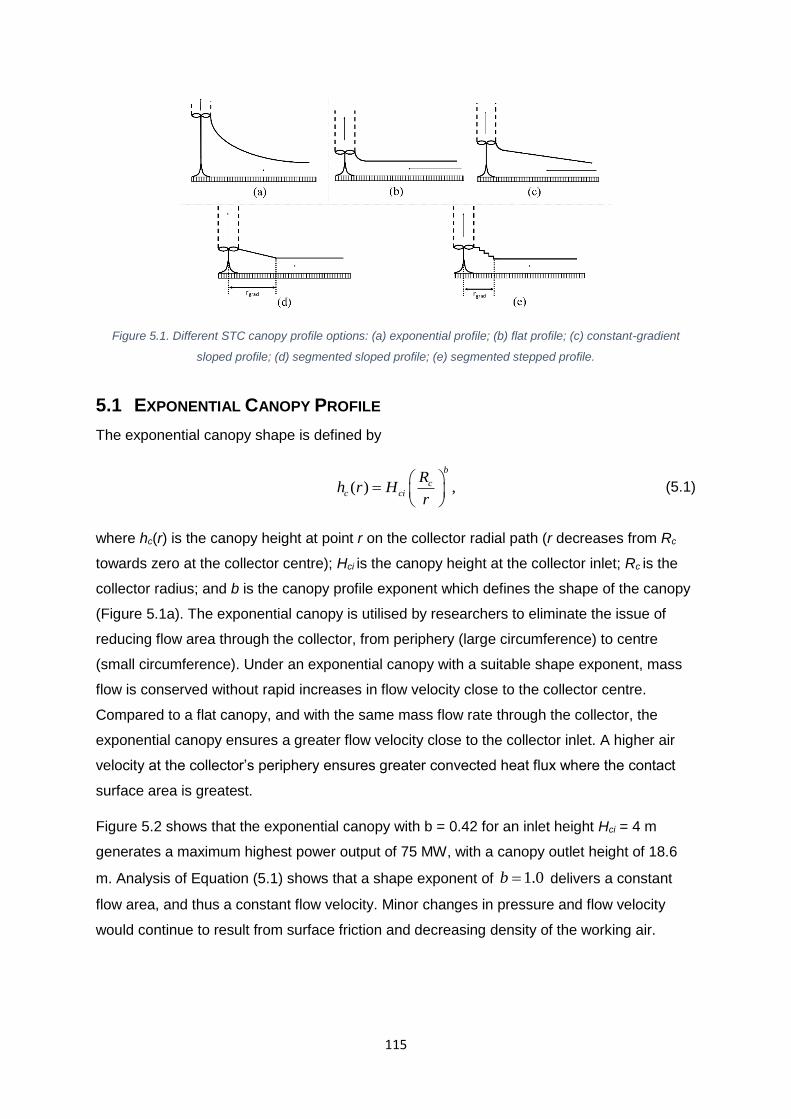
115
Figure 5.1. Different STC canopy profile options: (a) exponential profile; (b) flat profile; (c) constant-gradient
sloped profile; (d) segmented sloped profile; (e) segmented stepped profile.
5.1 EXPONENTIAL CANOPY PROFILE
The exponential canopy shape is defined by
) ,(
b
cc ci
Rr Hh
r
(5.1)
where hc(r) is the canopy height at point r on the collector radial path (r decreases from Rc
towards zero at the collector centre); Hci is the canopy height at the collector inlet; Rc is the
collector radius; and b is the canopy profile exponent which defines the shape of the canopy
(Figure 5.1a). The exponential canopy is utilised by researchers to eliminate the issue of
reducing flow area through the collector, from periphery (large circumference) to centre
(small circumference). Under an exponential canopy with a suitable shape exponent, mass
flow is conserved without rapid increases in flow velocity close to the collector centre.
Compared to a flat canopy, and with the same mass flow rate through the collector, the
exponential canopy ensures a greater flow velocity close to the collector inlet. A higher air
velocity at the collector’s periphery ensures greater convected heat flux where the contact
surface area is greatest.
Figure 5.2 shows that the exponential canopy with b = 0.42 for an inlet height Hci = 4 m
generates a maximum highest power output of 75 MW, with a canopy outlet height of 18.6
m. Analysis of Equation (5.1) shows that a shape exponent of 1.0b delivers a constant
flow area, and thus a constant flow velocity. Minor changes in pressure and flow velocity
would continue to result from surface friction and decreasing density of the working air.

116
Figure 5.2. Change in power output with canopy exponent for the reference STC with an exponential canopy. Canopy outlet height given for reference (Hci = 4 m, I = 900 Wm-2, T∞ = 305 K).
This configuration delivers the highest air velocity at the collector periphery, compared to
other values of shape exponent b . However, air velocity at the collector outlet is greatest
when 0b , assuming a constant mass flow rate through both configurations. Hence, there
are two counteracting factors which must be optimised to find the greatest power output –
large shape exponents lead to higher velocities (and thus greater heat transfer to the
working air) at the collector periphery; whereas small shape exponents lead to higher
velocities towards the collector outlet.
Further relevant points include the circular collector geometry, which dictates that collector
surface contact area (ground and canopy underside) decreases with the square of the radial
position, reducing the available area across which heat is transferred to the air. Additionally,
a change in collector canopy profile will necessarily change the mass flow rate through the
system, as the canopy profile affects the temperature and velocity of the air at the collector
outlet. Hence, only when using a fixed constant mass flow rate to compare exponential-
canopy collectors does the shape exponent 1b return as being optimum.
There is yet a further factor. Altering the value of exponent b changes the collector outlet
height (up to 156mco
h for 1b ), thereby altering the geometry of the collector-to-chimney
transition section (see Figure 5.2).

117
Changing the dimensions of the transition section, specifically the ratio of collector outlet flow
area to chimney inlet flow area, has an impact upon flow velocity according to
co
chi co
chi
Av
Av (5.2)
(repeated from Chapter 3), and upon static pressure according to
2
2 12
co cochi co co
chi
gHp
Ap
Av
(5.3)
(repeated from Chapter 3), where subscript co denotes flow properties and geometry at the
collector outlet, and subscript chi denotes the same at the chimney inlet. The process is
assumed to be isothermal, and is modelled here using the Bernoulli equation for a flow
within an adiabatic streamtube. Equations (5.2) and (5.3) illustrate how increasing the
collector outlet height not only changes the air flow properties within the collector, but also
changes the air velocity and air pressure at the chimney inlet (prior to passing through the
turbines).
The ratio of collector outlet flow area to chimney inlet flow area is therefore an important
parameter which determines the best-performing exponential canopy profile. There are three
important cases, each considered here in turn. They are:
1. 1co
chi
A
A : The chimney inlet air velocity will be less than that of the collector outlet.
The ratio of flow areas drives a change in flow velocity, which, by Bernoulli, causes
an increase in chimney inlet air pressure. Additionally, there is a minor counter-effect
(a reduction in chimney inlet air pressure) due to a small gain in height potential
between the collector outlet and chimney inlet. Under the condition 1co
chi
A
A , we can
state that
.2
cochi co
gHpp
(5.4)

118
2. 1co
chi
A
A : In this case the flow areas are equal. The chimney inlet air velocity is
equal to the collector outlet air velocity and the chimney inlet air pressure is reduced
from the collector outlet air pressure only by the gain in gravitational potential
.2
cochi co
gHpp
(5.5)
3. 1co
chi
A
A : In this case the flow area constricts between the collector outlet and
chimney inlet. Air velocity is correspondingly increased at the chimney inlet. Air
pressure at the chimney inlet is always less than air pressure at the collector outlet:
.2
cochi co
gHpp
(5.6)
All other things being equal, a reduction in chimney inlet air pressure delivers
increased power output (the best-performing exponential profile had a ratio
0.678co
chi
A
A ), but this is counteracted by reduced heat gain from the collector for the
reasons outlined above.
A collector inlet height of 4 m and a canopy exponent of b = 1.0 would lead to an outlet
height of 156 m for the reference STC plant dimensions. Such a large canopy outlet height,
coupled with the complex canopy shape, would make design, manufacture and maintenance
of the collector prohibitively complicated and therefore costly. Although not simulated in this
model, losses due to ambient wind displacing working air beneath the canopy (see Chapter
2) are reduced when using the exponential canopy due to its potential for lower canopy
height at the collector periphery and greater air velocities at the periphery, compared to other
canopy profiles.
5.2 FLAT CANOPY PROFILE
The flat canopy has the same height throughout the collector (Figure 5.1b), and has the
advantage of being simple and relatively cheap to construct and maintain (for moderate
heights at least). Due to its simplicity, it has been used for many physical prototypes, not
least the Manzanares STC plant (Haaf et al. [6]). Varying the canopy height, it was found
that STC performance peaks at Hc = 9 m and P = 63 MW, or 85% of the best-performing
exponential canopy (Figure 5.3). Such a height is tall enough to make construction and
maintenance difficult.
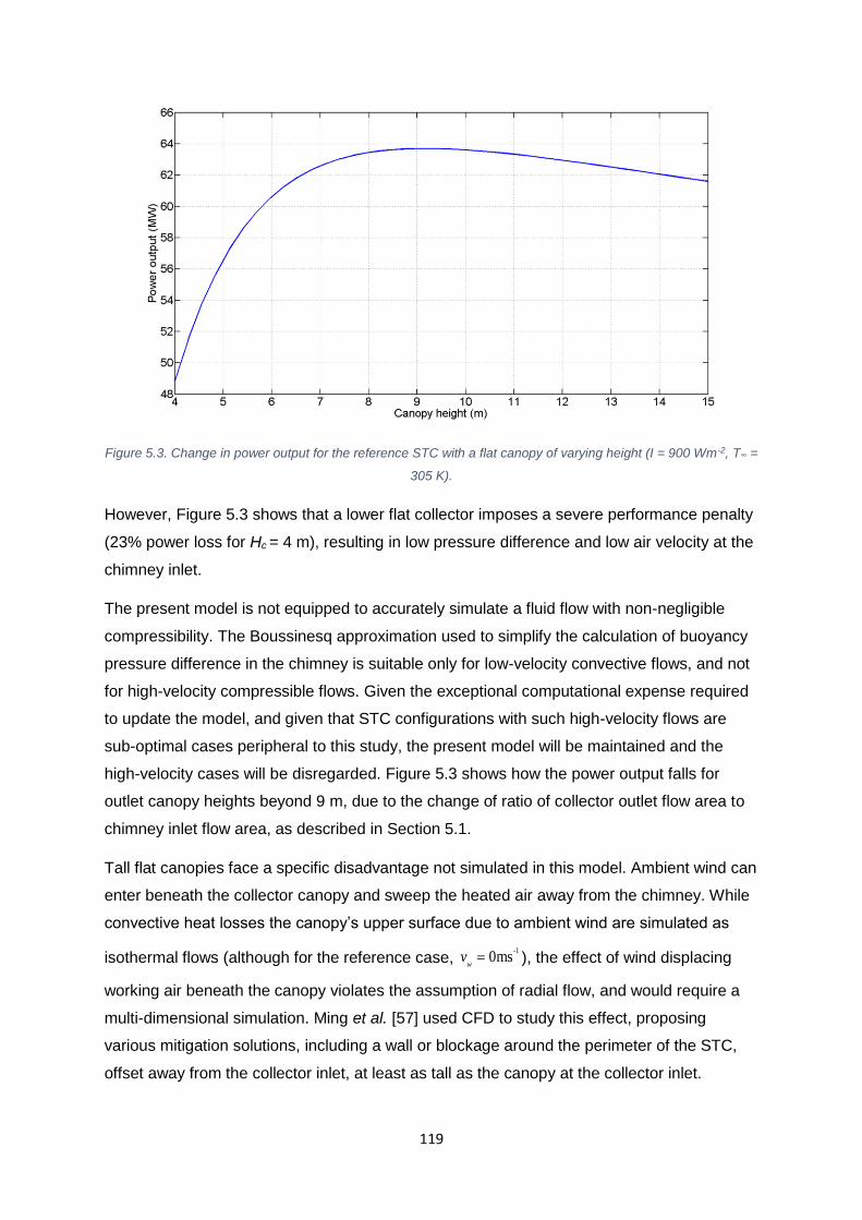
119
Figure 5.3. Change in power output for the reference STC with a flat canopy of varying height (I = 900 Wm-2, T∞ =
305 K).
However, Figure 5.3 shows that a lower flat collector imposes a severe performance penalty
(23% power loss for Hc = 4 m), resulting in low pressure difference and low air velocity at the
chimney inlet.
The present model is not equipped to accurately simulate a fluid flow with non-negligible
compressibility. The Boussinesq approximation used to simplify the calculation of buoyancy
pressure difference in the chimney is suitable only for low-velocity convective flows, and not
for high-velocity compressible flows. Given the exceptional computational expense required
to update the model, and given that STC configurations with such high-velocity flows are
sub-optimal cases peripheral to this study, the present model will be maintained and the
high-velocity cases will be disregarded. Figure 5.3 shows how the power output falls for
outlet canopy heights beyond 9 m, due to the change of ratio of collector outlet flow area to
chimney inlet flow area, as described in Section 5.1.
Tall flat canopies face a specific disadvantage not simulated in this model. Ambient wind can
enter beneath the collector canopy and sweep the heated air away from the chimney. While
convective heat losses the canopy’s upper surface due to ambient wind are simulated as
isothermal flows (although for the reference case, -1
0msw
v ), the effect of wind displacing
working air beneath the canopy violates the assumption of radial flow, and would require a
multi-dimensional simulation. Ming et al. [57] used CFD to study this effect, proposing
various mitigation solutions, including a wall or blockage around the perimeter of the STC,
offset away from the collector inlet, at least as tall as the canopy at the collector inlet.
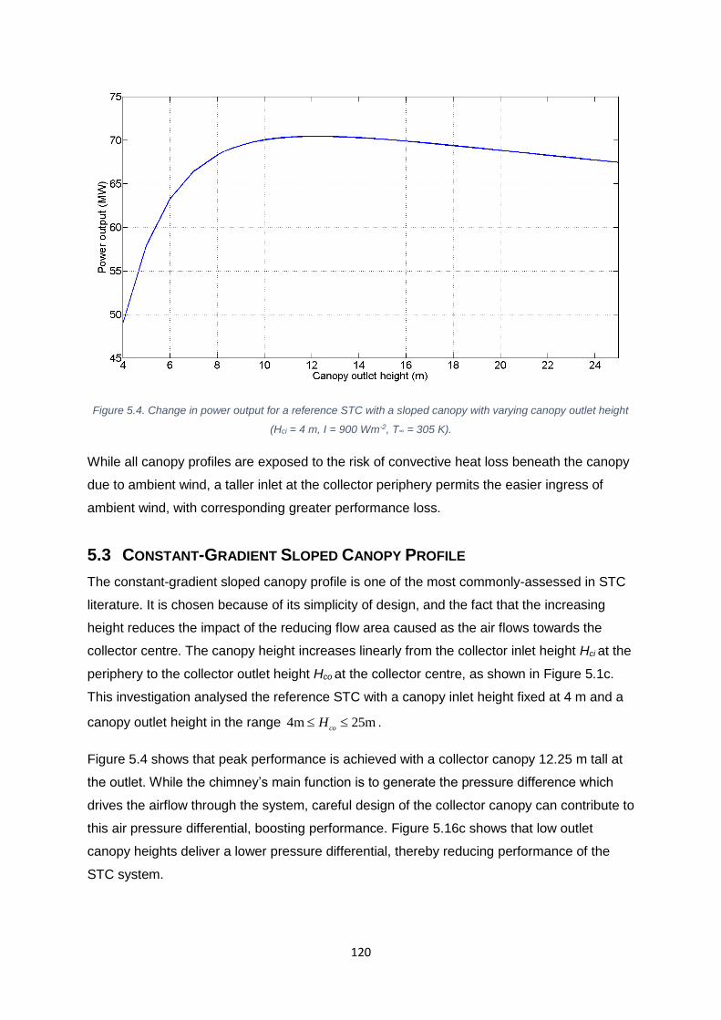
120
Figure 5.4. Change in power output for a reference STC with a sloped canopy with varying canopy outlet height
(Hci = 4 m, I = 900 Wm-2, T∞ = 305 K).
While all canopy profiles are exposed to the risk of convective heat loss beneath the canopy
due to ambient wind, a taller inlet at the collector periphery permits the easier ingress of
ambient wind, with corresponding greater performance loss.
5.3 CONSTANT-GRADIENT SLOPED CANOPY PROFILE
The constant-gradient sloped canopy profile is one of the most commonly-assessed in STC
literature. It is chosen because of its simplicity of design, and the fact that the increasing
height reduces the impact of the reducing flow area caused as the air flows towards the
collector centre. The canopy height increases linearly from the collector inlet height Hci at the
periphery to the collector outlet height Hco at the collector centre, as shown in Figure 5.1c.
This investigation analysed the reference STC with a canopy inlet height fixed at 4 m and a
canopy outlet height in the range m 25m4co
H .
Figure 5.4 shows that peak performance is achieved with a collector canopy 12.25 m tall at
the outlet. While the chimney’s main function is to generate the pressure difference which
drives the airflow through the system, careful design of the collector canopy can contribute to
this air pressure differential, boosting performance. Figure 5.16c shows that low outlet
canopy heights deliver a lower pressure differential, thereby reducing performance of the
STC system.
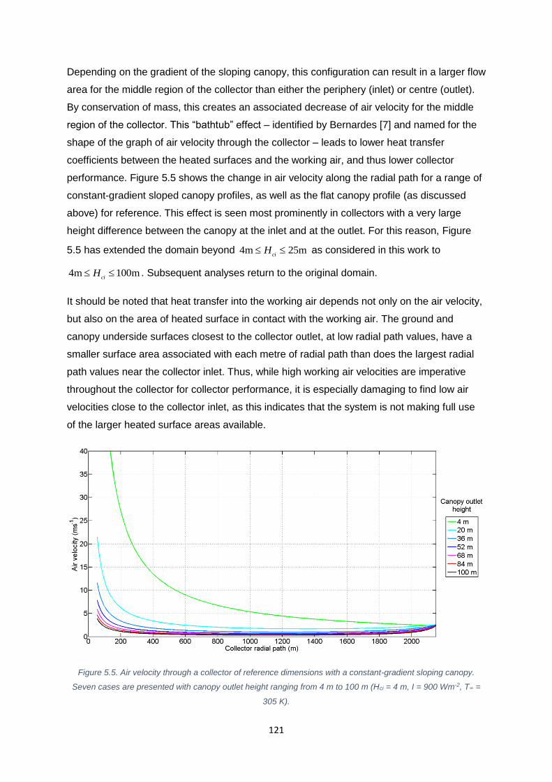
121
Depending on the gradient of the sloping canopy, this configuration can result in a larger flow
area for the middle region of the collector than either the periphery (inlet) or centre (outlet).
By conservation of mass, this creates an associated decrease of air velocity for the middle
region of the collector. This “bathtub” effect – identified by Bernardes [7] and named for the
shape of the graph of air velocity through the collector – leads to lower heat transfer
coefficients between the heated surfaces and the working air, and thus lower collector
performance. Figure 5.5 shows the change in air velocity along the radial path for a range of
constant-gradient sloped canopy profiles, as well as the flat canopy profile (as discussed
above) for reference. This effect is seen most prominently in collectors with a very large
height difference between the canopy at the inlet and at the outlet. For this reason, Figure
5.5 has extended the domain beyond m 25m4ci
H as considered in this work to
m 100m4ci
H . Subsequent analyses return to the original domain.
It should be noted that heat transfer into the working air depends not only on the air velocity,
but also on the area of heated surface in contact with the working air. The ground and
canopy underside surfaces closest to the collector outlet, at low radial path values, have a
smaller surface area associated with each metre of radial path than does the largest radial
path values near the collector inlet. Thus, while high working air velocities are imperative
throughout the collector for collector performance, it is especially damaging to find low air
velocities close to the collector inlet, as this indicates that the system is not making full use
of the larger heated surface areas available.
Figure 5.5. Air velocity through a collector of reference dimensions with a constant-gradient sloping canopy.
Seven cases are presented with canopy outlet height ranging from 4 m to 100 m (Hci = 4 m, I = 900 Wm-2, T∞ =
305 K).
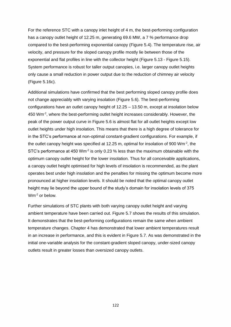
122
For the reference STC with a canopy inlet height of 4 m, the best-performing configuration
has a canopy outlet height of 12.25 m, generating 69.6 MW, a 7 % performance drop
compared to the best-performing exponential canopy (Figure 5.4). The temperature rise, air
velocity, and pressure for the sloped canopy profile mostly lie between those of the
exponential and flat profiles in line with the collector height (Figure 5.13 - Figure 5.15).
System performance is robust for taller output canopies, i.e. larger canopy outlet heights
only cause a small reduction in power output due to the reduction of chimney air velocity
(Figure 5.16c).
Additional simulations have confirmed that the best performing sloped canopy profile does
not change appreciably with varying insolation (Figure 5.6). The best-performing
configurations have an outlet canopy height of 12.25 – 13.50 m, except at insolation below
450 Wm-2, where the best-performing outlet height increases considerably. However, the
peak of the power output curve in Figure 5.6 is almost flat for all outlet heights except low
outlet heights under high insolation. This means that there is a high degree of tolerance for
in the STC’s performance at non-optimal constant-gradient configurations. For example, if
the outlet canopy height was specified at 12.25 m, optimal for insolation of 900 Wm-2, the
STC’s performance at 450 Wm-2 is only 0.23 % less than the maximum obtainable with the
optimum canopy outlet height for the lower insolation. Thus for all conceivable applications,
a canopy outlet height optimised for high levels of insolation is recommended, as the plant
operates best under high insolation and the penalties for missing the optimum become more
pronounced at higher insolation levels. It should be noted that the optimal canopy outlet
height may lie beyond the upper bound of the study’s domain for insolation levels of 375
Wm-2 or below.
Further simulations of STC plants with both varying canopy outlet height and varying
ambient temperature have been carried out. Figure 5.7 shows the results of this simulation.
It demonstrates that the best-performing configurations remain the same when ambient
temperature changes. Chapter 4 has demonstrated that lower ambient temperatures result
in an increase in performance, and this is evident in Figure 5.7. As was demonstrated in the
initial one-variable analysis for the constant-gradient sloped canopy, under-sized canopy
outlets result in greater losses than oversized canopy outlets.

123
Figure 5.6. Power output for reference STC with constant-gradient canopy and changing canopy outlet height,
simulated for varying insolation. Hci = 4 m; T∞ = 305 K; Rc = 2150 m; Hch = 1000 m; Rc = 55 m.
Figure 5.7. Power output for reference STC with constant-gradient canopy and changing canopy outlet height,
simulated for varying ambient temperature. Hci = 4 m; I = 900 Wm-2; Rc = 2150 m; Hch = 1000 m; Rc = 55 m.
5.4 SEGMENTED CANOPY PROFILE
The rationale behind this canopy profile was to develop a profile shape delivering the
performance benefits of the constant-gradient and exponential canopies while limiting the
additional cost due to increased construction complexity. The segmented canopy profile is
flat at the outer periphery, rising linearly from radial point rgrad up to the chimney (Figure
5.1d). The effect of changing the location of rgrad has been investigated, keeping the inlet

124
height and the outlet height as those of the best performing constant-gradient profile (Hci = 4
m, Hco = 11.5 m).
The best-performing configuration (rgrad = 650 m at -2900WmI ) generates 73 MW power
(Figure 5.8), 8.7 % higher than the constant-gradient profile and equal to the best-performing
exponential collector, without the same canopy height requirements at the chimney outlet.
In order to investigate the robustness of the optimum configuration, the power output was
calculated for varying environmental conditions, as shown in Figure 5.9 & Figure 5.10.
Power output increases with increasing insolation, and the value of rgrad giving a maximum
power output changes from 750mgrad
r in the insolation range -2 -2375Wm 675WmI , to
650mgrad
r for insolation greater than 675 Wm-2.
Very low insolation results in a much larger value for optimum gradr . In this study, an
insolation of 300 Wm-2 produces an optimum gradr of 1100 m (Figure 5.9). The optima for
different levels of insolation are very flat, and at low insolation ( -2375WmI ), installing a
segmented canopy with 750mgrad
r leads to a performance loss of only 0.3 % if the point of
gradient change were constructed at 1100mgrad
r (best-performing for -2300WmI ).
Figure 5.8. Change in power output for a reference STC with a segmented canopy profile (Hci = 4 m, I = 900 Wm-
2, T∞ = 305 K).
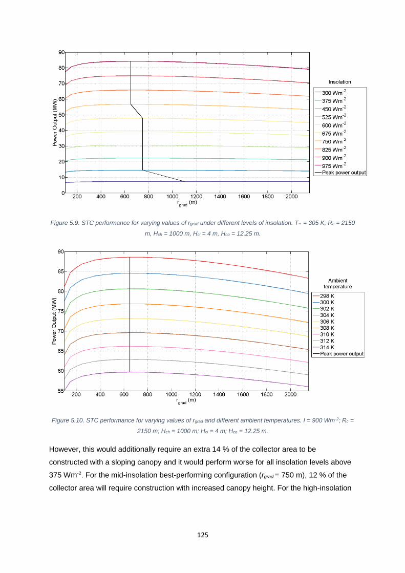
125
Figure 5.9. STC performance for varying values of rgrad under different levels of insolation. T∞ = 305 K, Rc = 2150
m, Hch = 1000 m, Hci = 4 m, Hco = 12.25 m.
Figure 5.10. STC performance for varying values of rgrad and different ambient temperatures. I = 900 Wm-2; Rc =
2150 m; Hch = 1000 m; Hci = 4 m; Hco = 12.25 m.
However, this would additionally require an extra 14 % of the collector area to be
constructed with a sloping canopy and it would perform worse for all insolation levels above
375 Wm-2. For the mid-insolation best-performing configuration (rgrad = 750 m), 12 % of the
collector area will require construction with increased canopy height. For the high-insolation
126
best-performing configuration ( 650mgrad
r ), only 9 % of the collector area will require a
sloped canopy.
The value of rgrad yielding optimum power output is not sensitive to ambient temperature, as
shown by Figure 5.10. The optimum value of rgrad remains fixed at 650 m across a range of
ambient temperatures ( K 314K298 T
). The optimum remains relatively flat, indicating only
minor performance penalties for specifying a value for rgrad other than 650 m.
The air velocity (and thus mass flow rate) at the chimney for this configuration approximately
matches that of the constant-gradient and exponential canopies, but the pressure drop is
slightly lower (Figure 5.16d). Figure 5.14 shows the increased air velocity under the flat part
of the canopy (to 355 m), which then gradually approaches the constant-gradient case. This
leads to a small pressure increase due to the change in canopy profile (Figure 5.15), which
is partially balanced by the slightly higher air temperature rise (Figure 5.13). By keeping the
collector height low for the majority of the flow path, the segmented collector canopy ensures
that higher air velocities are maintained within the collector (Figure 5.14), inducing higher
rates of heat transfer from the ground and canopy underside surface. The reduction in air
velocity found within linearly-sloped canopies (identified by Bernardes [7]) is not observed in
Figure 5.14 as the chosen configurations of each canopy design are the best-performing of
their type and hence do not exhibit this behaviour.
One of the aims of this investigation is to provide cost-effective performance enhancements
by modifying the canopy design. A canopy with rgrad = 265 m is proposed as a compromise
between construction costs and power output, for which only 1.5 % of the collector area has
a gradient. This will provide a power output of 72 MW, only a 2 % performance loss
compared to the best-performing exponential canopy and less than a 1 % loss compared to
the best-performing segmented canopy.
5.5 STEPPED CANOPY PROFILE
A linearly-sloped canopy section would require a double curvature – it must encircle the
chimney at the collector centre and also slope upwards towards the centre, like the top
surface of a shallow cone. It is unlikely that such a construction would be built from curved
pieces of glass to match exactly the curvature specified – it is considered more likely that the
double-curvature will be approximated with a series of flat panels. In the same vein, the
sloped and segmented sloped canopies could be constructed as a series of horizontal
annular canopy sections joined by short transition sections, as shown in Figure 5.1e. To
investigate such a design, the sloping region of the segmented profile was approximated by
127
steps of different heights such that the volume under the canopy remains approximately the
same. The transition between these steps is modelled as a vertical increase in height, but
could equally be constructed as a short sloping region to reduce recirculation losses.
A segmented, stepped canopy profile with Hci = 4 m, rgrad = 265 m and hstep = 2.75 m (i.e.
consisting of three equal-height steps from hc = 4.0 m to 6.75 m at rc = 265 m; from hc = 6.75
m to 9.50 m at rc = 195 m; and from hc = 9.50 m to 12.25 m at rc = 125 m), generates 71 MW
power output, only 5 % less than the best-performing case and only 2 % less than the same
segmented profile without the steps. Figure 5.14 shows that the air velocity curve follows
that of the segmented profile with jumps associated with each step in the collector height.
Figure 5.15 shows the matching behaviour in the pressure profiles due to the canopy height
jumps with a slightly higher pressure at the collector outlet responsible for the marginal
reduction in output power. Therefore the stepped profile offers the same performance
advantages as the segmented profile – that of maintaining a low canopy height for the
majority of the collector radial path to boost air velocity and thus heat transfer – but with
reduced construction complexity.
5.6 OPTIMUM RGRAD SENSITIVITY TO PLANT DIMENSIONS
This chapter has determined the optimum location for gradr , noting that STC performance is
relatively insensitive to changes in gradr , except close to the chimney inlet. The optimum
gradr
is insensitive to ambient temperature and while it does change with insolation, the penalty for
missing the optimum is consistently minor.
This section will consider the optimum position of gradr for a STC of dimensions other than
the reference dimensions used thus far. The investigation evaluates STC performance for
three collector radii and three chimney heights. For each parameter, the three values chosen
represent 50 % of the reference value, the reference value itself, and 150 % of the reference
value.

128
Figure 5.11. Performance of the reference STC with a collector of varying radius Rc and varying change-of-
gradient point rgrad, which is normalised against Rc on the x-axis. I = 900 Wm-2; T∞ = 305K; Hch = 1000m; Hci =
3m; Hco = 7m.
Figure 5.12. Performance of the reference STC with a chimney of varying height Hch and varying change-of-
gradient point rgrad. I = 900 Wm-2; T∞ = 305K; Rc = 2150m; Hci = 3m; Hco = 7m.
Figure 5.11 shows the sensitivity of power output to normalised gradr , for different collector
radii. The power output returned varies little as rgrad is varied along the collector radial path,
denoting relative insensitivity to gradr position. The optimum rgrad is also shown to vary little,
returning an optimum normalised rgrad of 0.50c
R to 0.55c
R depending on collector radius.
This indicates that engineers designing a commercial-scale STC plant for construction can
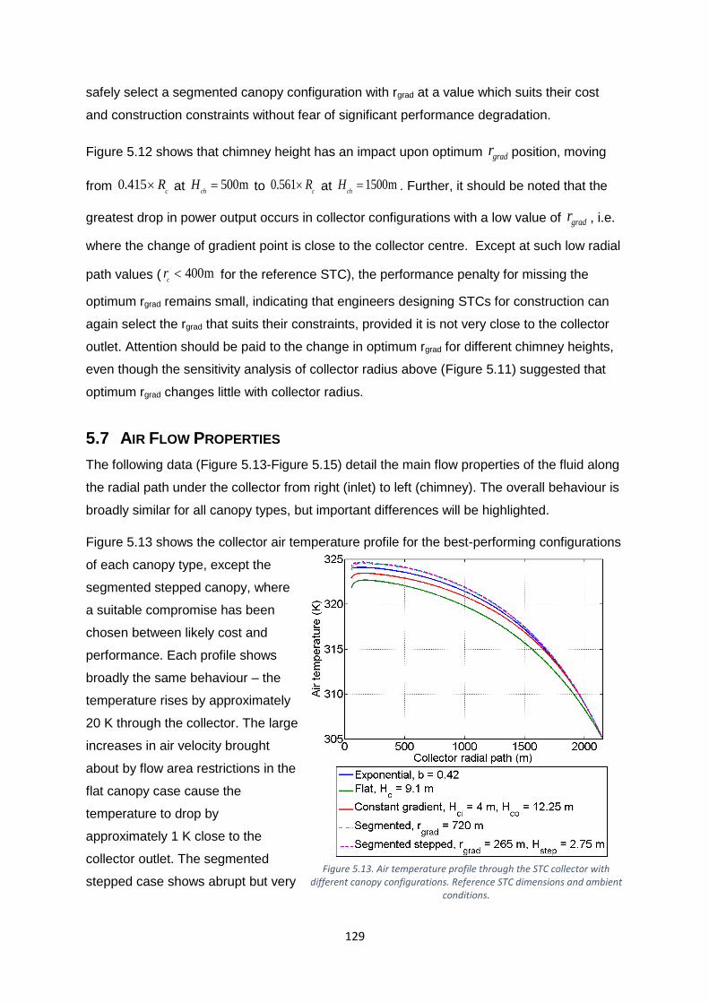
129
safely select a segmented canopy configuration with rgrad at a value which suits their cost
and construction constraints without fear of significant performance degradation.
Figure 5.12 shows that chimney height has an impact upon optimum gradr position, moving
from 0.415c
R at 500mch
H to 0.561c
R at 1500mch
H . Further, it should be noted that the
greatest drop in power output occurs in collector configurations with a low value of gradr , i.e.
where the change of gradient point is close to the collector centre. Except at such low radial
path values ( 400mc
r for the reference STC), the performance penalty for missing the
optimum rgrad remains small, indicating that engineers designing STCs for construction can
again select the rgrad that suits their constraints, provided it is not very close to the collector
outlet. Attention should be paid to the change in optimum rgrad for different chimney heights,
even though the sensitivity analysis of collector radius above (Figure 5.11) suggested that
optimum rgrad changes little with collector radius.
5.7 AIR FLOW PROPERTIES
The following data (Figure 5.13-Figure 5.15) detail the main flow properties of the fluid along
the radial path under the collector from right (inlet) to left (chimney). The overall behaviour is
broadly similar for all canopy types, but important differences will be highlighted.
Figure 5.13 shows the collector air temperature profile for the best-performing configurations
of each canopy type, except the
segmented stepped canopy, where
a suitable compromise has been
chosen between likely cost and
performance. Each profile shows
broadly the same behaviour – the
temperature rises by approximately
20 K through the collector. The large
increases in air velocity brought
about by flow area restrictions in the
flat canopy case cause the
temperature to drop by
approximately 1 K close to the
collector outlet. The segmented
stepped case shows abrupt but very Figure 5.13. Air temperature profile through the STC collector with
different canopy configurations. Reference STC dimensions and ambient conditions.
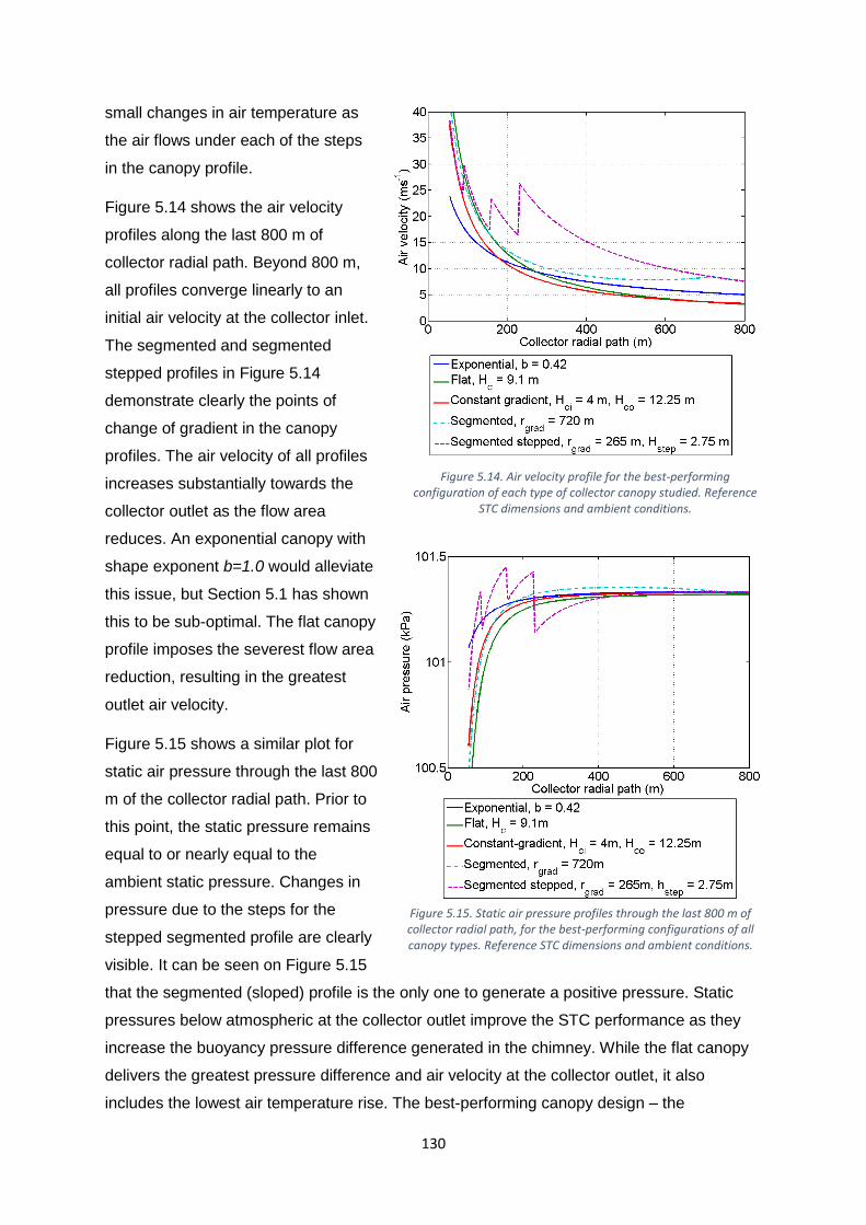
130
small changes in air temperature as
the air flows under each of the steps
in the canopy profile.
Figure 5.14 shows the air velocity
profiles along the last 800 m of
collector radial path. Beyond 800 m,
all profiles converge linearly to an
initial air velocity at the collector inlet.
The segmented and segmented
stepped profiles in Figure 5.14
demonstrate clearly the points of
change of gradient in the canopy
profiles. The air velocity of all profiles
increases substantially towards the
collector outlet as the flow area
reduces. An exponential canopy with
shape exponent b=1.0 would alleviate
this issue, but Section 5.1 has shown
this to be sub-optimal. The flat canopy
profile imposes the severest flow area
reduction, resulting in the greatest
outlet air velocity.
Figure 5.15 shows a similar plot for
static air pressure through the last 800
m of the collector radial path. Prior to
this point, the static pressure remains
equal to or nearly equal to the
ambient static pressure. Changes in
pressure due to the steps for the
stepped segmented profile are clearly
visible. It can be seen on Figure 5.15
that the segmented (sloped) profile is the only one to generate a positive pressure. Static
pressures below atmospheric at the collector outlet improve the STC performance as they
increase the buoyancy pressure difference generated in the chimney. While the flat canopy
delivers the greatest pressure difference and air velocity at the collector outlet, it also
includes the lowest air temperature rise. The best-performing canopy design – the
Figure 5.14. Air velocity profile for the best-performing configuration of each type of collector canopy studied. Reference
STC dimensions and ambient conditions.
Figure 5.15. Static air pressure profiles through the last 800 m of collector radial path, for the best-performing configurations of all canopy types. Reference STC dimensions and ambient conditions.

131
exponential canopy – delivers the smallest pressure difference and the lowest air velocity,
but it has the highest air temperature at the collector outlet. The segmented stepped canopy,
considered simpler and cheaper to build, delivers the same outlet air temperature as the
segmented canopy, without the excessively tall outlet canopy height. As such, the
segmented stepped canopy is recommended as the best-performing easily-constructed
canopy profile.
5.8 AIR PROPERTIES AT THE CHIMNEY INLET
Chapter 3 shows that the power output of the system is dependent upon the product of the
volume flow rate of working air through the turbines and the pressure drop across the
turbines. Maximising power output therefore depends upon maximising the air velocity and
pressure potential at the chimney inlet. Figure 5.16 shows the air velocity and pressure
potential for each of the canopy profiles under consideration. Note that while the pressure
potential generated would typically be described as a negative pressure difference (as it
generates buoyancy), it is given in Figure 5.16 as a positive pressure difference to maintain
the same convention as the air velocity.
Figure 5.16 gives insight into how the power output for each STC configuration is derived.
For example, it can be seen from Figure 5.16a that the best-performing exponential
configuration, with shape exponent b=0.42, is decided mainly by the air velocity at the
chimney inlet and not the pressure difference. Figure 5.16b shows the condition of the air at
the chimney inlet for a STC with a flat canopy. Despite the high air velocity at the collector
outlet for this configuration (see Figure 5.14), the air velocities achieved at the chimney inlet
are lower than all other profiles, regardless of canopy height. As the canopy height is
increased, so the ratio co
chi
A
A increases, causing a lower air velocity and higher pressure
(lower pressure difference) at the chimney inlet. These undesirable effects are avoided in
other canopy profiles.
The constant-gradient sloped canopy yields almost identical pressure differences at the
chimney inlet (Figure 5.16c), but the chimney inlet air velocity is improved compared to that
for the flat canopy. Examination of Figure 5.13 shows that the constant-gradient canopy
delivers air temperature approximately 1 K higher than the flat canopy (both with best-
performing configurations for their canopy type). Herein lies the advantage delivered by the
constant-gradient canopy, reflected in the higher power output.
Examining all cases in Figure 5.16 shows that the pressure difference rises from an initial
low value to reach a plateau. For the segmented canopy profile (Figure 5.16d), the initial rise
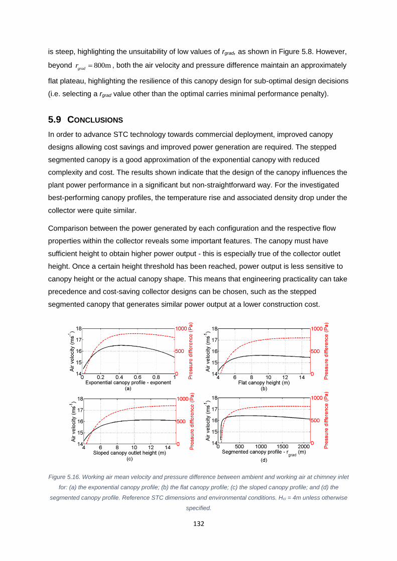
132
is steep, highlighting the unsuitability of low values of rgrad, as shown in Figure 5.8. However,
beyond 800mgrad
r , both the air velocity and pressure difference maintain an approximately
flat plateau, highlighting the resilience of this canopy design for sub-optimal design decisions
(i.e. selecting a rgrad value other than the optimal carries minimal performance penalty).
5.9 CONCLUSIONS
In order to advance STC technology towards commercial deployment, improved canopy
designs allowing cost savings and improved power generation are required. The stepped
segmented canopy is a good approximation of the exponential canopy with reduced
complexity and cost. The results shown indicate that the design of the canopy influences the
plant power performance in a significant but non-straightforward way. For the investigated
best-performing canopy profiles, the temperature rise and associated density drop under the
collector were quite similar.
Comparison between the power generated by each configuration and the respective flow
properties within the collector reveals some important features. The canopy must have
sufficient height to obtain higher power output - this is especially true of the collector outlet
height. Once a certain height threshold has been reached, power output is less sensitive to
canopy height or the actual canopy shape. This means that engineering practicality can take
precedence and cost-saving collector designs can be chosen, such as the stepped
segmented canopy that generates similar power output at a lower construction cost.
Figure 5.16. Working air mean velocity and pressure difference between ambient and working air at chimney inlet
for: (a) the exponential canopy profile; (b) the flat canopy profile; (c) the sloped canopy profile; and (d) the
segmented canopy profile. Reference STC dimensions and environmental conditions. Hci = 4m unless otherwise
specified.

133
For canopies with sufficient height, the plant power output curves in Figure 5.2, Figure 5.3,
Figure 5.4 and Figure 5.8 follow closely the chimney inlet velocity shown in Figure 5.2. This
means that the collector to chimney transition is important and that the mass flow rate is the
key driver for increased power generation.
The STC model detailed in Chapter 3 has been utilised here to assess the power output for
various canopy profiles. This highlighted the importance of sufficiently increasing the cross-
sectional flow area near the chimney to prevent pressure losses. Existing literature has
focussed mainly on canopy profiles which are either flat, sloped at a constant gradient, or
exponential. Flat canopies are simple to design, but cause pressure losses due to the
restriction of the air flow cross section, especially close to the chimney.
A constant-gradient sloped canopy can improve power output. The exponential canopy
profile brings performance improvements, but construction and maintenance could be
difficult and costly due to access issues.
For the best-performing design of each canopy type, the temperature rise and associated
density drop under the collector were found to be quite similar. The canopy outlet height has
been identified as an important parameter, as it defines the pressure drop in the flow through
the collector-to-chimney transition section. This highlighted the importance of sufficiently
increasing the cross-sectional flow area near the chimney to prevent pressure losses.
This study proposes instead a segmented canopy profile which is flat from the collector
periphery to a point rgrad on the radial path, from which the canopy height increases with a
constant gradient or in flat steps. The segmented canopy profile matches the power output
of the best-performing exponential profile and uses a simpler design, reducing both
construction and maintenance costs. The stepped, segmented canopy profile with a sensible
choice for the location of rgrad is likely to provide a good ratio of power output to construction
cost. The segmented canopy design is highly robust for a variety of environmental
conditions. Further such construction-friendly designs should be developed and tested as
STC technology moves towards commercial deployment.

134
6 SUSPENDED CHIMNEYS: LITERATURE REVIEW AND
MOTIVATION
This literature review is motivated by the suggestion that the chimney component of solar
thermal chimney power plants is difficult to construct and represents a major risk to investors
in an STC power plant. Generally speaking, a commercial-scale STC will require a chimney
between 500 m and 1500 m tall, with an internal flow diameter of 100 m to 600 m. Being
located at the centre of a solar collector, the chimney should be constructed with as thin a
wall as possible and safe. The chimney must be able to support its own self-weight and
withstand wind loading. Given the excessive material consumption and high level of
engineering risk associated with deploying conventional materials and construction
techniques for this new class of thin-walled structure, radical alternatives are being
considered. This project will investigate the feasibility of constructing a chimney (or the top
part of the chimney) from engineered fabrics and holding it aloft either under positive air
pressure or with a lighter-than-air gas, nominally helium.
In order to understand the limitations of conventional materials in constructing the STC
chimney component, this chapter presents a review of literature concerning the structural
aspects of STC design. (Chapter 2 considered only the thermo-fluid dynamical aspects.) The
present chapter provides an overview of literature on wind loading, and a review of
theoretical and experimental literature on the behaviour of inflatable beams under load, as
this is the best approximation currently available for the behaviour of a suspended chimney.
Additionally, this chapter will present a review of literature which has determined
experimentally the constitutive properties of fabric materials used in similar structures.
6.1 SOLAR THERMAL CHIMNEY POWER PLANTS – CHIMNEY CONSTRUCTION
& ANALYSIS The solar thermal chimney power plant is attractive in part due to its simplicity, consisting as
it does of only three key components: the solar collector, the turbine and the chimney. Both
the solar collector and the turbines are relatively conventional components, albeit of rather
large size. The chimney, however, is unconventional by virtue of its size. Thin-shell slender
structures up to 1000 m tall introduce several engineering challenges which must be met.
This section considers the challenges posed and the research community’s current
response.
Tall chimneys face a series of loads which they must safely withstand. These include the
component’s own weight; the pressure profiles imposed by mean wind loading (external) and
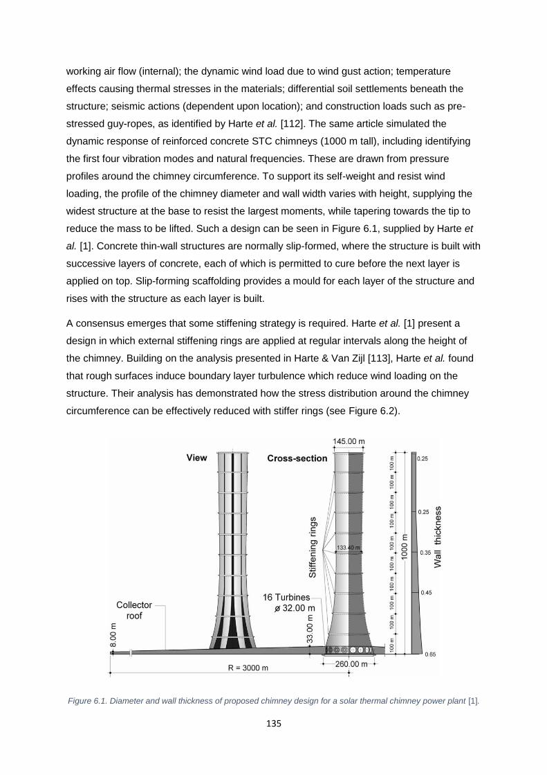
135
working air flow (internal); the dynamic wind load due to wind gust action; temperature
effects causing thermal stresses in the materials; differential soil settlements beneath the
structure; seismic actions (dependent upon location); and construction loads such as pre-
stressed guy-ropes, as identified by Harte et al. [112]. The same article simulated the
dynamic response of reinforced concrete STC chimneys (1000 m tall), including identifying
the first four vibration modes and natural frequencies. These are drawn from pressure
profiles around the chimney circumference. To support its self-weight and resist wind
loading, the profile of the chimney diameter and wall width varies with height, supplying the
widest structure at the base to resist the largest moments, while tapering towards the tip to
reduce the mass to be lifted. Such a design can be seen in Figure 6.1, supplied by Harte et
al. [1]. Concrete thin-wall structures are normally slip-formed, where the structure is built with
successive layers of concrete, each of which is permitted to cure before the next layer is
applied on top. Slip-forming scaffolding provides a mould for each layer of the structure and
rises with the structure as each layer is built.
A consensus emerges that some stiffening strategy is required. Harte et al. [1] present a
design in which external stiffening rings are applied at regular intervals along the height of
the chimney. Building on the analysis presented in Harte & Van Zijl [113], Harte et al. found
that rough surfaces induce boundary layer turbulence which reduce wind loading on the
structure. Their analysis has demonstrated how the stress distribution around the chimney
circumference can be effectively reduced with stiffer rings (see Figure 6.2).
Figure 6.1. Diameter and wall thickness of proposed chimney design for a solar thermal chimney power plant [1].
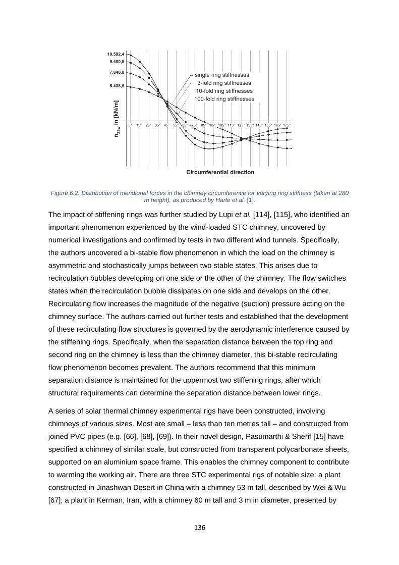
136
Figure 6.2. Distribution of meridional forces in the chimney circumference for varying ring stiffness (taken at 280 m height), as produced by Harte et al. [1].
The impact of stiffening rings was further studied by Lupi et al. [114], [115], who identified an
important phenomenon experienced by the wind-loaded STC chimney, uncovered by
numerical investigations and confirmed by tests in two different wind tunnels. Specifically,
the authors uncovered a bi-stable flow phenomenon in which the load on the chimney is
asymmetric and stochastically jumps between two stable states. This arises due to
recirculation bubbles developing on one side or the other of the chimney. The flow switches
states when the recirculation bubble dissipates on one side and develops on the other.
Recirculating flow increases the magnitude of the negative (suction) pressure acting on the
chimney surface. The authors carried out further tests and established that the development
of these recirculating flow structures is governed by the aerodynamic interference caused by
the stiffening rings. Specifically, when the separation distance between the top ring and
second ring on the chimney is less than the chimney diameter, this bi-stable recirculating
flow phenomenon becomes prevalent. The authors recommend that this minimum
separation distance is maintained for the uppermost two stiffening rings, after which
structural requirements can determine the separation distance between lower rings.
A series of solar thermal chimney experimental rigs have been constructed, involving
chimneys of various sizes. Most are small – less than ten metres tall – and constructed from
joined PVC pipes (e.g. [66], [68], [69]). In their novel design, Pasumarthi & Sherif [15] have
specified a chimney of similar scale, but constructed from transparent polycarbonate sheets,
supported on an aluminium space frame. This enables the chimney component to contribute
to warming the working air. There are three STC experimental rigs of notable size: a plant
constructed in Jinashwan Desert in China with a chimney 53 m tall, described by Wei & Wu
[67]; a plant in Kerman, Iran, with a chimney 60 m tall and 3 m in diameter, presented by

137
Gholamalizadeh & Mansouri [71]; and the Manzanares STC power plant, which operated in
Spain in the 1980s [6], and had a chimney 195 m tall and 10 m in diameter. The first of
these, in the Jinashwan Desert, was constructed using conventional reinforced concrete.
Gholamalizadeh & Mansouri provide no data on the construction methods of their
experimental plant in Iran. The Manzanares structure was constructed from a series of
corrugated iron rings, which were installed by raising the rings already on site and securing
the next ring at the base. While the Manzanares chimney was installed using novel
construction methods, other experimental STC plants have utilised readily-available
materials which have suited their small scale. Schlaich, Bergermann und Partner, a German
civil engineering consultancy which constructed the Manzanares STC plant, used the plant
as an opportunity to evaluate their novel construction methods. The sheer size of
commercial-scale STC chimneys makes their method unlikely to be used on commercial
plants.
Brief analyses of suspended inflatable chimney structures have already been undertaken.
Papageorgiou has filed a patent on the suspended chimney concept [116]. His design - as
introduced in Papageorgiou [118] - consists of stiff, high-strength fabrics to which helium-
filled tori are affixed to provide lift. High-pressure, small-diameter air-filled tori are affixed to
the structure to provide strength (see Figure 6.3). In his analysis, Papageorgiou is expecting
to withstand wind loading by permitting the floating chimney to lean under wind load, while
supplying a hinge mechanism at the base to obviate the need to withstand large moments at
the ground connection (Figure 6.4).
Figure 6.3. Design details of proposed floating chimney design [119].
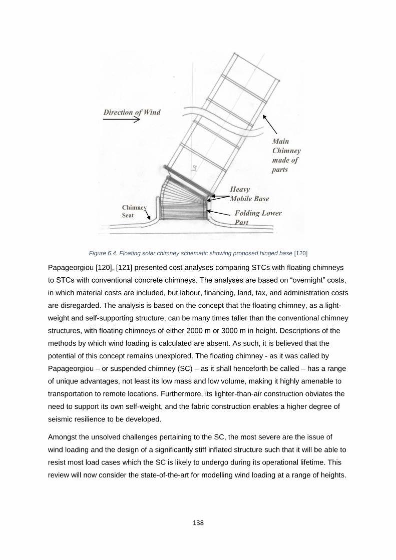
138
Figure 6.4. Floating solar chimney schematic showing proposed hinged base [120]
Papageorgiou [120], [121] presented cost analyses comparing STCs with floating chimneys
to STCs with conventional concrete chimneys. The analyses are based on “overnight” costs,
in which material costs are included, but labour, financing, land, tax, and administration costs
are disregarded. The analysis is based on the concept that the floating chimney, as a light-
weight and self-supporting structure, can be many times taller than the conventional chimney
structures, with floating chimneys of either 2000 m or 3000 m in height. Descriptions of the
methods by which wind loading is calculated are absent. As such, it is believed that the
potential of this concept remains unexplored. The floating chimney - as it was called by
Papageorgiou – or suspended chimney (SC) – as it shall henceforth be called – has a range
of unique advantages, not least its low mass and low volume, making it highly amenable to
transportation to remote locations. Furthermore, its lighter-than-air construction obviates the
need to support its own self-weight, and the fabric construction enables a higher degree of
seismic resilience to be developed.
Amongst the unsolved challenges pertaining to the SC, the most severe are the issue of
wind loading and the design of a significantly stiff inflated structure such that it will be able to
resist most load cases which the SC is likely to undergo during its operational lifetime. This
review will now consider the state-of-the-art for modelling wind loading at a range of heights.
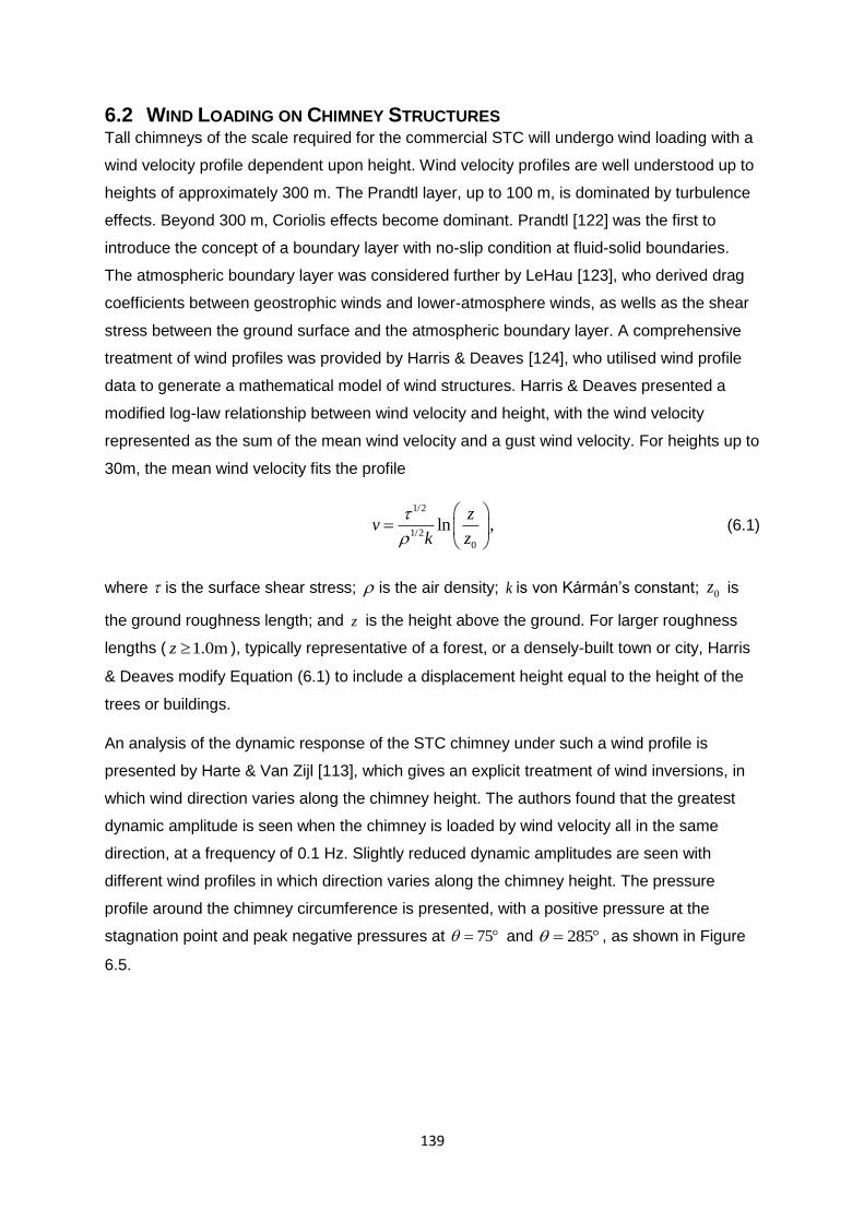
139
6.2 WIND LOADING ON CHIMNEY STRUCTURES Tall chimneys of the scale required for the commercial STC will undergo wind loading with a
wind velocity profile dependent upon height. Wind velocity profiles are well understood up to
heights of approximately 300 m. The Prandtl layer, up to 100 m, is dominated by turbulence
effects. Beyond 300 m, Coriolis effects become dominant. Prandtl [122] was the first to
introduce the concept of a boundary layer with no-slip condition at fluid-solid boundaries.
The atmospheric boundary layer was considered further by LeHau [123], who derived drag
coefficients between geostrophic winds and lower-atmosphere winds, as wells as the shear
stress between the ground surface and the atmospheric boundary layer. A comprehensive
treatment of wind profiles was provided by Harris & Deaves [124], who utilised wind profile
data to generate a mathematical model of wind structures. Harris & Deaves presented a
modified log-law relationship between wind velocity and height, with the wind velocity
represented as the sum of the mean wind velocity and a gust wind velocity. For heights up to
30m, the mean wind velocity fits the profile
1/2
1/2
0
ln ,z
vk z
(6.1)
where is the surface shear stress; is the air density; k is von Kármán’s constant; 0z is
the ground roughness length; and z is the height above the ground. For larger roughness
lengths ( 1.0mz ), typically representative of a forest, or a densely-built town or city, Harris
& Deaves modify Equation (6.1) to include a displacement height equal to the height of the
trees or buildings.
An analysis of the dynamic response of the STC chimney under such a wind profile is
presented by Harte & Van Zijl [113], which gives an explicit treatment of wind inversions, in
which wind direction varies along the chimney height. The authors found that the greatest
dynamic amplitude is seen when the chimney is loaded by wind velocity all in the same
direction, at a frequency of 0.1 Hz. Slightly reduced dynamic amplitudes are seen with
different wind profiles in which direction varies along the chimney height. The pressure
profile around the chimney circumference is presented, with a positive pressure at the
stagnation point and peak negative pressures at 75 and 285 , as shown in Figure
6.5.
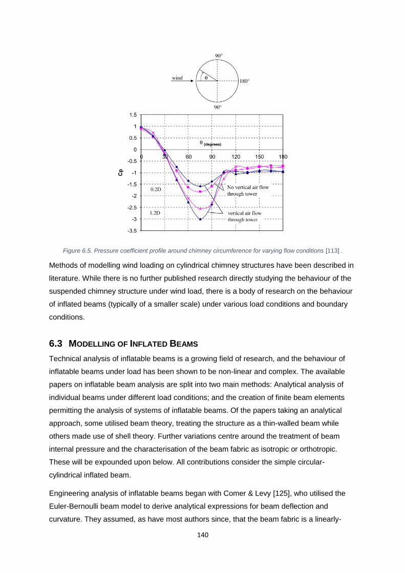
140
Figure 6.5. Pressure coefficient profile around chimney circumference for varying flow conditions [113] .
Methods of modelling wind loading on cylindrical chimney structures have been described in
literature. While there is no further published research directly studying the behaviour of the
suspended chimney structure under wind load, there is a body of research on the behaviour
of inflated beams (typically of a smaller scale) under various load conditions and boundary
conditions.
6.3 MODELLING OF INFLATED BEAMS
Technical analysis of inflatable beams is a growing field of research, and the behaviour of
inflatable beams under load has been shown to be non-linear and complex. The available
papers on inflatable beam analysis are split into two main methods: Analytical analysis of
individual beams under different load conditions; and the creation of finite beam elements
permitting the analysis of systems of inflatable beams. Of the papers taking an analytical
approach, some utilised beam theory, treating the structure as a thin-walled beam while
others made use of shell theory. Further variations centre around the treatment of beam
internal pressure and the characterisation of the beam fabric as isotropic or orthotropic.
These will be expounded upon below. All contributions consider the simple circular-
cylindrical inflated beam.
Engineering analysis of inflatable beams began with Comer & Levy [125], who utilised the
Euler-Bernoulli beam model to derive analytical expressions for beam deflection and
curvature. They assumed, as have most authors since, that the beam fabric is a linearly-

141
elastic membrane capable of carrying tension, but no compressive loads. Their analysis
identified the wrinkling load – the load at which the first discontinuity in the membrane
surface would occur – as the point of zero resultant stress. Their beam deflection model did
not contain a term for the internal pressure of the beam, signalling that further work may be
required.
Main et al. [126] developed an analytical model capable of simulating a circular-cylindrical
inflated beam up to the point of wrinkling, concluding that the behaviour was identical to a
solid linearly-elastic beam, provided the membrane remained unwrinkled. The authors
carried out a series of experiments to validate their analytical model and established that the
model was reasonably accurate provided the slenderness ratio (diameter/length) was not too
low. However, for such thin-walled beams, the shear deformation was shown by Fichter
[127] to be non-negligible. His model treated the beam as a linearly elastic Timoshenko
element, and he was able to derive linearised equations for deflection, curvature and
membrane stress. Steeves [128] took a similar approach in his study of the behaviour of
inflatable beams for the US Army.
Wielgosz & Thomas [129] presented an analytical study of the behaviour of inflated fabric
panels at high pressure. Their formulation involves Timoshenko beam theory, with the
equilibrium equations written for the beam in the deformed state, to account for pressure
follower forces acting on the internal surfaces of the membrane. Timoshenko beam theory
includes an additional degree of freedom that is neglected in Euler-Bernoulli beam theory.
This manifests as permitting beam cross-sections to rotate relative to the neutral axis,
whereas under Euler-Bernoulli, they remain perpendicular to the neutral axis. Both methods
assume that planar sections remain plane, i.e. there is no out-of-plane buckling of the cross-
section. Furthermore, Wielgosz & Thomas assume that internal pressure remains constant
regardless of membrane shape (that is, regardless of any changes in internal volume). To
validate their analytical model, Wielgosz and Thomas undertook practical experiments,
measuring the load required to achieve a given deflection for a dropstitch panel. Wielgosz &
Thomas utilise only highly-inflated panels, in the range of 1 – 3 bar gauge pressure. The
same authors published another contribution in which they applied their analytical model to a
circular-cylindrical beam, in lieu of a panel [130].
A series of analyses began with a study by Ligarò & Barsotti [131] extending the deflection
algorithm proposed by Main et al. [126] by developing novel equations for the moment of
inertia of wrinkled cross-sections. A set of non-linear equations is derived and must be
solved iteratively to find the beam behaviour under load. The authors successfully
demonstrate how Euler-Bernoulli beam models are insufficient for inflatable beams,
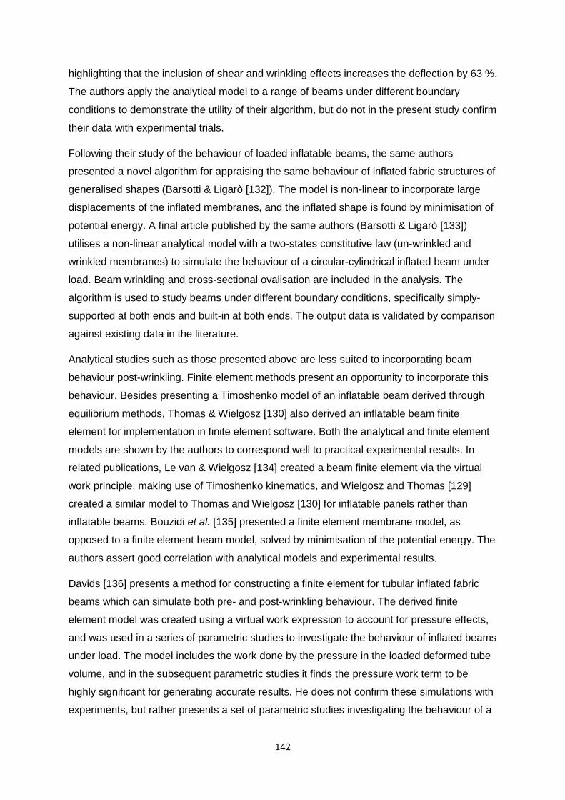
142
highlighting that the inclusion of shear and wrinkling effects increases the deflection by 63 %.
The authors apply the analytical model to a range of beams under different boundary
conditions to demonstrate the utility of their algorithm, but do not in the present study confirm
their data with experimental trials.
Following their study of the behaviour of loaded inflatable beams, the same authors
presented a novel algorithm for appraising the same behaviour of inflated fabric structures of
generalised shapes (Barsotti & Ligarò [132]). The model is non-linear to incorporate large
displacements of the inflated membranes, and the inflated shape is found by minimisation of
potential energy. A final article published by the same authors (Barsotti & Ligarò [133])
utilises a non-linear analytical model with a two-states constitutive law (un-wrinkled and
wrinkled membranes) to simulate the behaviour of a circular-cylindrical inflated beam under
load. Beam wrinkling and cross-sectional ovalisation are included in the analysis. The
algorithm is used to study beams under different boundary conditions, specifically simply-
supported at both ends and built-in at both ends. The output data is validated by comparison
against existing data in the literature.
Analytical studies such as those presented above are less suited to incorporating beam
behaviour post-wrinkling. Finite element methods present an opportunity to incorporate this
behaviour. Besides presenting a Timoshenko model of an inflatable beam derived through
equilibrium methods, Thomas & Wielgosz [130] also derived an inflatable beam finite
element for implementation in finite element software. Both the analytical and finite element
models are shown by the authors to correspond well to practical experimental results. In
related publications, Le van & Wielgosz [134] created a beam finite element via the virtual
work principle, making use of Timoshenko kinematics, and Wielgosz and Thomas [129]
created a similar model to Thomas and Wielgosz [130] for inflatable panels rather than
inflatable beams. Bouzidi et al. [135] presented a finite element membrane model, as
opposed to a finite element beam model, solved by minimisation of the potential energy. The
authors assert good correlation with analytical models and experimental results.
Davids [136] presents a method for constructing a finite element for tubular inflated fabric
beams which can simulate both pre- and post-wrinkling behaviour. The derived finite
element model was created using a virtual work expression to account for pressure effects,
and was used in a series of parametric studies to investigate the behaviour of inflated beams
under load. The model includes the work done by the pressure in the loaded deformed tube
volume, and in the subsequent parametric studies it finds the pressure work term to be
highly significant for generating accurate results. He does not confirm these simulations with
experiments, but rather presents a set of parametric studies investigating the behaviour of a

143
simply-supported inflated beam loaded with a central point force. While noting that fabric
properties E and G change with pressure, he assumes constant values for his parametric
study. The values chosen are exceptionally low compared to Thomas & Wielgosz [130]
(Davids: E = 0.625 N/m, G = 0.012 N/m; Thomas & Wielgosz: E = 230 000 N/m, G = 110
000 N/m). He analyses beam mid-span displacement at a range of pressures, both with and
without the work done by pressure. Including the work done by pressure produces a
significantly reduced deflection beyond the wrinkling load.
Davids [137] complements this analysis with a further work formulating a finite element
model of a beam element again using Timoshenko kinematics and the virtual work principle,
also including work done by volume change within the beam’s fabric envelope. The authors
assume that pressure remains constant to simplify the analysis, and justify their assumption
by noting that the anticipated change in pressure is very small as a proportion of the
pressure within the inflated structure. This work extends upon [136] by validating the
presented model against a series of 4-point load experiments. Good agreement was
achieved between experimental and numerical results. The authors also studied the
inflatable beam as an axially-loaded column, comparing their experimental results to their
own model, the Euler-Bernoulli beam model and the model presented by Fichter [127]. They
found that including shear effects and the p V work term were essential in obtaining an
accurate model of the beam under load, especially for low slenderness ratios (wide
columns).
Veldman [138] and Veldman et al. [139] treated the inflatable beam as a very thin shell
rather than a membrane, arguing that the shell can have zero net pressure, i.e. be inflated to
ambient pressure, and still carry a lateral load. Membrane analysis does not permit a zero-
positive-pressure beam to resist a load. Furthermore, under membrane analysis, the
wrinkling load is established independently of material properties through a simple
relationship dependent only upon material thickness and beam radius, whereas shell theory
will permit variation in wrinkling loads dependent upon the material used.
The debate between most authors in the field centres around the application of shell theory
versus membrane theory as a means of approximating the fabric surface. A third option
exists, explored by a minority of researchers. This route focuses on the mechanics of the
woven fabrics and looks at inter-tow mechanics, or the friction between threads. An analysis
of inter-tow mechanics is supplied by Kabche et al. [140], in which the authors describe an
experimental procedure for obtaining constitutive properties for a range of materials under a
range of conditions not by loading the inflated member as a beam (as in Cavallaro et al.
[141]), but rather as a column, with compressive and torsional loads applied. The data

144
obtained are used as inputs to a finite element model of an inflatable beam and good
correlation with the experimental results are obtained, leading the authors to suggest that
their method for obtaining constitutive properties has yielded accurate data. As with
Cavallaro et al. [141], the authors noted that material moduli increase with increasing internal
pressure of the beam.
6.4 EXPERIMENTAL TESTING OF INFLATABLE BEAMS The simulation of inflatable beams has proven to be significantly more complex than that of
beams built from traditional materials. Many researchers have chosen to carry out practical
experiments, either to validate and augment their modelling efforts, or as the main
investigative method to gain a greater insight into the behaviour of inflatable beams. All the
literature surveyed as part of this work utilised the simple circular-cross-section beam. The
most comprehensive studies begin by investigating the constitutive properties of the fabrics
used to manufacture the beams (e.g. Kabche et al. [140] and Clapp et al. [142]).
Experiments to establish constitutive properties require bi-axial testing to establish stress-
strain and yield strength. Loads are applied slowly to prevent creep and specially-designed
jaws prevent fabric slipping in the test rigs. The constitutive data is used within the models
created by the authors, which are then validated against subsequent experiments measuring
beam deflection.
Many authors have carried out practical experiments measuring the deflection of inflated
beams (e.g. Wicker [143]; Thomas & Wielgosz [130]; Cavallaro et al. [144]; and Davids &
Zhang [137]). Wicker [143] carried out a series of experimental tests without formally
deriving a model against which to compare them, instead testing novel materials and
comparing them to existing fabric and conventional materials. It was found that while the
strength and stiffness of inflated structures was improving with new materials, their
performance still lay behind conventional steel frame structures. Across the surveyed
literature, in the experiments the inflated beams are simply-supported and tested with three-
point or four-point loading. The supports which connect to the inflatable beam range from
contact pads to specially-constructed clamps which ensure that the load is distributed across
the fabric cross-section and that the axis of rotation lies on the neutral axis of the beam (see
Figure 6.6 from Thomas & Wielgosz [130]). Loads are applied in various ways, including the
use of a winch beneath the beam connected to a cable, which connects to the beam with a
belt or a built-in hook. Alternatively, the beam is secured with three or four simple supports
between two jaws which are opened or closed to generate a load on the structure (e.g.
Cavallaro et al. [144]). The experimental rigs described herein have provided researchers
with a means to accurately apply a given load to their inflatable beams.

145
Figure 6.6. Three-point loading of a simply-supported inflated beam with custom supports to prevent asymmetrical loading of beam cross-section [130].
They must also have a means of accurately measuring the deflection of the loaded beams.
In the case of extending or contracting a set of jaws, an Instron machine can both measure
load and displacement of the jaws.
Where the experimental procedures are used as a means of validating accompanying
models, the method of measuring deflection is not always made clear. A comprehensive
means of recording the displacement of a fabric beam’s surface following the application of
load is supplied by Clapp et al. [142], who utilised digital image correlation to record the
strain field across the whole fabric surface when the beam was loaded longitudinally (i.e.
treated as a column). From this method, they uncovered spatial variation of shear stress in
the beam’s fabric surface.
6.5 INFLATABLE STRUCTURES UNDER WIND LOADING The study of fluid-structure interaction (FSI) has applications in, for example,
geoengineering, naval architecture and renewable energy. Inflatable structures, currently
suitable for a range of niche applications, are normally assessed for wind interaction by
conventional CFD methods, in which the loading upon the inflated structure is expressed
without considering the potential large deflections which inflated structures can undergo
without failure. A more comprehensive analysis would include the deformation of the inflated
structure and the resulting change in wind loading upon the structure. The coupled nature of
these two phenomena complicates such an analysis.
Sygulski produced a range of studies investigating the behaviour of a hemispherical inflated
membrane subject to external wind loads. In [145], [146], Sygulski developed a boundary
element method to simulate surface vibrations of an air-inflated sphere. It is assumed that
the air is compressible and inviscid. The developed model was validated with wind tunnel
experiments [147].
Spinelli [148] developed a shooting-type dynamic model of an air-inflated cylinder under
wind load. The model evaluates cylinder deflection and deformation over a relatively short
time period (23 seconds), and is shown by the author to demonstrate good stability. The
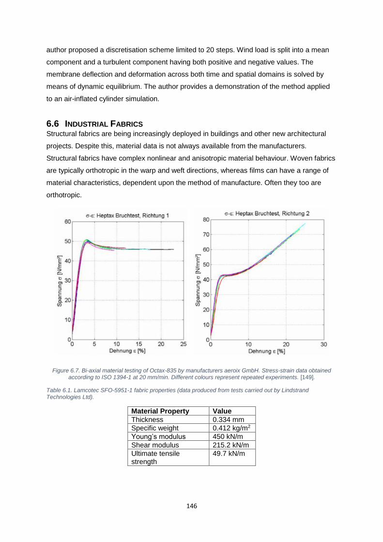
146
author proposed a discretisation scheme limited to 20 steps. Wind load is split into a mean
component and a turbulent component having both positive and negative values. The
membrane deflection and deformation across both time and spatial domains is solved by
means of dynamic equilibrium. The author provides a demonstration of the method applied
to an air-inflated cylinder simulation.
6.6 INDUSTRIAL FABRICS Structural fabrics are being increasingly deployed in buildings and other new architectural
projects. Despite this, material data is not always available from the manufacturers.
Structural fabrics have complex nonlinear and anisotropic material behaviour. Woven fabrics
are typically orthotropic in the warp and weft directions, whereas films can have a range of
material characteristics, dependent upon the method of manufacture. Often they too are
orthotropic.
Figure 6.7. Bi-axial material testing of Octax-835 by manufacturers aeroix GmbH. Stress-strain data obtained according to ISO 1394-1 at 20 mm/min. Different colours represent repeated experiments. [149].
Table 6.1. Lamcotec SFO-5951-1 fabric properties (data produced from tests carried out by Lindstrand
Technologies Ltd).
Material Property Value
Thickness 0.334 mm
Specific weight 0.412 kg/m2
Young’s modulus 450 kN/m
Shear modulus 215.2 kN/m
Ultimate tensile strength
49.7 kN/m
147
This project is concerned chiefly with the lightweight helium-tight Octax 835, a film material
used to construct the first suspended chimney prototype; and with Lamcotec SFO-5951-1,
the woven and coated material used to manufacture the second-generation SC prototype.
Both prototypes are introduced in Chapter 7. The orthotropic nature of the Octax material is
evident from Figure 6.7, which shows greater material strength in direction 2 (Richtung 2)
than direction 1. Nonlinear behaviour is also exhibited. The material properties of the
Lamcotec fabric are shown in Table 6.1, obtained following extensive testing by Lindstrand
Technologies Ltd. All moduli are given as “membrane moduli” with units of force per unit
length, due to the membrane nature of the material.
6.7 SUMMARY Solar thermal chimney power plants require only three simple components: the solar
collector; the turbine & generator set; and the chimney. While each component presents
engineering challenges in scaling it up to the required size for commercial deployment, the
chimney presents the severest challenge. This review has presented the available literature
pertaining to the STC chimney component and the suspended chimney concept, particularly
under wind loading. While directly applicable research is limited, a range of methods have
been developed to model inflatable beams under load. These methods are both numerical
and analytical, and engage in particular with the nonlinear beam behaviour resulting from
loads which cause wrinkling discontinuities to develop in the beam fabric. Consensus has
broadly been reached that wrinkling occurs where the principal stresses in the fabric sum to
zero, although some researchers dissent, pointing out that this does not account for the state
in which the beam is fully inflated at ambient pressure.
The behaviour of inflated beams gives insight into the potential behaviour of the suspended
chimney, but the two cases cannot be considered identical. Specifically, while significant
research has been undertaken to establish the performance of a circular-cross-section
inflated beam, both pre- and post-wrinkling, there remains a dearth of research considering
different cross-sections. The suspended chimney has, by necessity, an annular cross-
section. Thus this review recommends that work is undertaken to establish the behaviour of
inflatable beams of different cross sections, and the dependence of beam response upon
different geometrical and material properties.
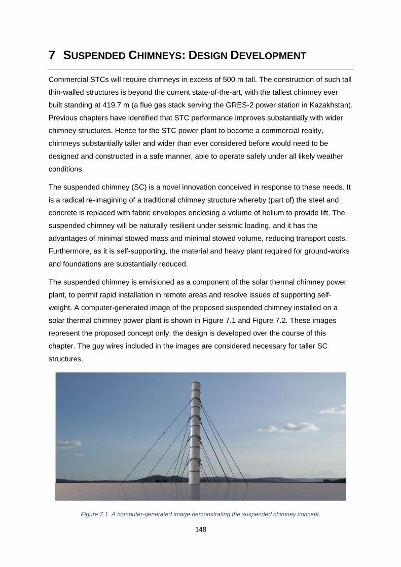
148
7 SUSPENDED CHIMNEYS: DESIGN DEVELOPMENT
Commercial STCs will require chimneys in excess of 500 m tall. The construction of such tall
thin-walled structures is beyond the current state-of-the-art, with the tallest chimney ever
built standing at 419.7 m (a flue gas stack serving the GRES-2 power station in Kazakhstan).
Previous chapters have identified that STC performance improves substantially with wider
chimney structures. Hence for the STC power plant to become a commercial reality,
chimneys substantially taller and wider than ever considered before would need to be
designed and constructed in a safe manner, able to operate safely under all likely weather
conditions.
The suspended chimney (SC) is a novel innovation conceived in response to these needs. It
is a radical re-imagining of a traditional chimney structure whereby (part of) the steel and
concrete is replaced with fabric envelopes enclosing a volume of helium to provide lift. The
suspended chimney will be naturally resilient under seismic loading, and it has the
advantages of minimal stowed mass and minimal stowed volume, reducing transport costs.
Furthermore, as it is self-supporting, the material and heavy plant required for ground-works
and foundations are substantially reduced.
The suspended chimney is envisioned as a component of the solar thermal chimney power
plant, to permit rapid installation in remote areas and resolve issues of supporting self-
weight. A computer-generated image of the proposed suspended chimney installed on a
solar thermal chimney power plant is shown in Figure 7.1 and Figure 7.2. These images
represent the proposed concept only, the design is developed over the course of this
chapter. The guy wires included in the images are considered necessary for taller SC
structures.
Figure 7.1. A computer-generated image demonstrating the suspended chimney concept.

149
Figure 7.2. A computer-generated image showing the suspended chimney from above.
7.1 INFLATABLE STRUCTURES – STATE-OF-THE-ART
Generally speaking, the deflection behaviour of an inflated beam under load is believed to
be linear with load until the fabric wrinkles, at which point the load-bearing capacity is
significantly reduced and behaviour becomes non-linear. Under further increased load, the
beam can collapse entirely, and load-bearing capacity reduces to zero.
The behaviour of inflatable beams under load has been simulated and tested experimentally,
using a range of comprehensive techniques. Almost all contributions have studied the
simplest beam configuration, with a circular cross-section. The development of a suspended
chimney will require the creation of an inflatable beam with an annular cross-section, and as
such this chapter intends to contribute to the state-of-the-art by presenting a design analysis
of a series of inflatable beams with this cross-section.
This chapter presents the development of the suspended chimneys through three prototypes
tested as part of this project (SC1, SC2, and SC3). Each prototype builds upon the lessons
learnt from the previous one, identifying and resolving issues of performance and
manufacturing. SC1 is a proof-of-concept prototype, manufactured from lightweight fabric
film and held aloft with helium gas. It contains no additional stiffening mechanism and serves
only to illustrate the proposed concept. SC2 and SC3 are both designed with the intention of
testing their behaviour under lateral load experimentally. SC2 is an air-filled prototype
manufactured from Précontraint 402 fabric which represents the stiffening components only
of a novel suspended chimney design. The helium volume is disregarded for this small-scale
prototype to reduce cost and resolve issues with scaling. Following design and
manufacturing lessons learned in the operation of SC2, a third prototype (SC3) was
specified and constructed. SC3 has a similar design to SC2, but improves upon a few
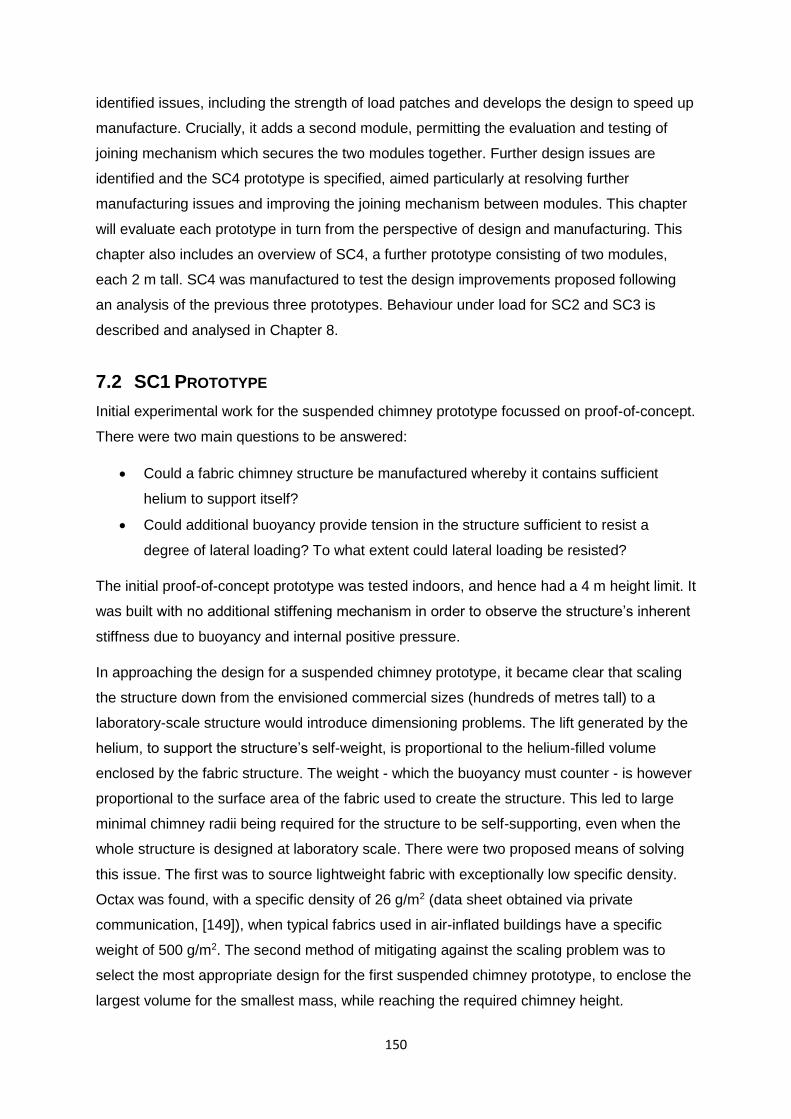
150
identified issues, including the strength of load patches and develops the design to speed up
manufacture. Crucially, it adds a second module, permitting the evaluation and testing of
joining mechanism which secures the two modules together. Further design issues are
identified and the SC4 prototype is specified, aimed particularly at resolving further
manufacturing issues and improving the joining mechanism between modules. This chapter
will evaluate each prototype in turn from the perspective of design and manufacturing. This
chapter also includes an overview of SC4, a further prototype consisting of two modules,
each 2 m tall. SC4 was manufactured to test the design improvements proposed following
an analysis of the previous three prototypes. Behaviour under load for SC2 and SC3 is
described and analysed in Chapter 8.
7.2 SC1 PROTOTYPE
Initial experimental work for the suspended chimney prototype focussed on proof-of-concept.
There were two main questions to be answered:
• Could a fabric chimney structure be manufactured whereby it contains sufficient
helium to support itself?
• Could additional buoyancy provide tension in the structure sufficient to resist a
degree of lateral loading? To what extent could lateral loading be resisted?
The initial proof-of-concept prototype was tested indoors, and hence had a 4 m height limit. It
was built with no additional stiffening mechanism in order to observe the structure’s inherent
stiffness due to buoyancy and internal positive pressure.
In approaching the design for a suspended chimney prototype, it became clear that scaling
the structure down from the envisioned commercial sizes (hundreds of metres tall) to a
laboratory-scale structure would introduce dimensioning problems. The lift generated by the
helium, to support the structure’s self-weight, is proportional to the helium-filled volume
enclosed by the fabric structure. The weight - which the buoyancy must counter - is however
proportional to the surface area of the fabric used to create the structure. This led to large
minimal chimney radii being required for the structure to be self-supporting, even when the
whole structure is designed at laboratory scale. There were two proposed means of solving
this issue. The first was to source lightweight fabric with exceptionally low specific density.
Octax was found, with a specific density of 26 g/m2 (data sheet obtained via private
communication, [149]), when typical fabrics used in air-inflated buildings have a specific
weight of 500 g/m2. The second method of mitigating against the scaling problem was to
select the most appropriate design for the first suspended chimney prototype, to enclose the
largest volume for the smallest mass, while reaching the required chimney height.
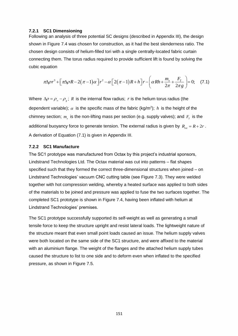
151
7.2.1 SC1 Dimensioning
Following an analysis of three potential SC designs (described in Appendix III), the design
shown in Figure 7.4 was chosen for construction, as it had the best slenderness ratio. The
chosen design consists of helium-filled tori with a single centrally-located fabric curtain
connecting them. The torus radius required to provide sufficient lift is found by solving the
cubic equation
3 2 02
2 ;2 1 12
x Tr R hm F
r R Rhg
r
(7.1)
Where g
; R is the internal flow radius; r is the helium torus radius (the
dependent variable); is the specific mass of the fabric (kg/m2); h is the height of the
chimney section; x
m is the non-lifting mass per section (e.g. supply valves); and T
F is the
additional buoyancy force to generate tension. The external radius is given by 2ext
R R r .
A derivation of Equation (7.1) is given in Appendix III.
7.2.2 SC1 Manufacture
The SC1 prototype was manufactured from Octax by this project’s industrial sponsors,
Lindstrand Technologies Ltd. The Octax material was cut into patterns – flat shapes
specified such that they formed the correct three-dimensional structures when joined – on
Lindstrand Technologies’ vacuum CNC cutting table (see Figure 7.3). They were welded
together with hot compression welding, whereby a heated surface was applied to both sides
of the materials to be joined and pressure was applied to fuse the two surfaces together. The
completed SC1 prototype is shown in Figure 7.4, having been inflated with helium at
Lindstrand Technologies’ premises.
The SC1 prototype successfully supported its self-weight as well as generating a small
tensile force to keep the structure upright and resist lateral loads. The lightweight nature of
the structure meant that even small point loads caused an issue. The helium supply valves
were both located on the same side of the SC1 structure, and were affixed to the material
with an aluminium flange. The weight of the flanges and the attached helium supply tubes
caused the structure to list to one side and to deform even when inflated to the specified
pressure, as shown in Figure 7.5.

152
Figure 7.3. Octax material on the vacuum CNC cutting table at Lindstrand Technologies Ltd, cutting patterns for
SC1 manufacture.
The helium leak rate proved to be unacceptably high, increasing further following fabric
creasing and repeated cycles of inflating and deflating. Despite its light weight, substantial
quantities of helium were still required to inflate the structure, resulting in inflation costs of
approximately £25 per inflation. After a few inflations and deflations, the helium leak rate had
increased to the point that the structure remained suitably inflated for only thirty minutes
following inflation.
Figure 7.4. The completed SC1 prototype inflated with helium at Lindstrand Technologies' premises.
Figure 7.5. Helium supply valve and tubing causing a point-load deflection and deformation of a torus on
the SC1.
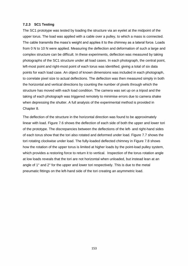
153
7.2.3 SC1 Testing
The SC1 prototype was tested by loading the structure via an eyelet at the midpoint of the
upper torus. The load was applied with a cable over a pulley, to which a mass is connected.
The cable transmits the mass’s weight and applies it to the chimney as a lateral force. Loads
from 0 N to 10 N were applied. Measuring the deflection and deformation of such a large and
complex structure can be difficult. In these experiments, deflection was measured by taking
photographs of the SC1 structure under all load cases. In each photograph, the central point,
left-most point and right-most point of each torus was identified, giving a total of six data
points for each load case. An object of known dimensions was included in each photograph,
to correlate pixel size to actual deflections. The deflection was then measured simply in both
the horizontal and vertical directions by counting the number of pixels through which the
structure has moved with each load condition. The camera was set up on a tripod and the
taking of each photograph was triggered remotely to minimise errors due to camera shake
when depressing the shutter. A full analysis of the experimental method is provided in
Chapter 8.
The deflection of the structure in the horizontal direction was found to be approximately
linear with load. Figure 7.6 shows the deflection of each side of both the upper and lower tori
of the prototype. The discrepancies between the deflections of the left- and right-hand sides
of each torus show that the tori also rotated and deformed under load. Figure 7.7 shows the
tori rotating clockwise under load. The fully-loaded deflected chimney in Figure 7.8 shows
how the rotation of the upper torus is limited at higher loads by the point-load pulley system,
which provides a restoring force to return it to vertical. Inspection of the torus rotation angle
at low loads reveals that the tori are not horizontal when unloaded, but instead lean at an
angle of 1° and 2° for the upper and lower tori respectively. This is due to the metal
pneumatic fittings on the left-hand side of the tori creating an asymmetric load.
154
Figure 7.6. Deflection (x-direction) of the left and right side of the upper and lower tori under progressively
increasing load.
Figure 7.7. Torus rotation under load. Note the initial non-zero
rotation due to the structure listing under the point-mass load of
the helium supply valves.
Figure 7.8. SC1 loaded at F=9.8N
Figure 7.9 shows the horizontal deformation of both the upper and lower tori. The upper
torus is stretched horizontally (increased diameter) due to the lateral loading, while the lower
torus is squeezed horizontally (reduced diameter) and stretched vertically (increased height)
due to a vertical component of the loading force. This vertical component arises as the
loading cable pulley remains at a fixed height level with the unloaded height of the upper
torus eyelet.
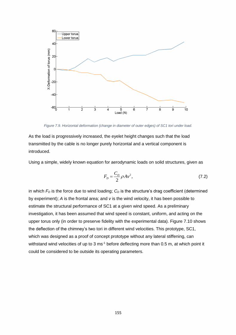
155
Figure 7.9. Horizontal deformation (change in diameter of outer edges) of SC1 tori under load.
As the load is progressively increased, the eyelet height changes such that the load
transmitted by the cable is no longer purely horizontal and a vertical component is
introduced.
Using a simple, widely known equation for aerodynamic loads on solid structures, given as
2
2,D
D
CF Av (7.2)
in which FD is the force due to wind loading; CD is the structure’s drag coefficient (determined
by experiment); A is the frontal area; and v is the wind velocity, it has been possible to
estimate the structural performance of SC1 at a given wind speed. As a preliminary
investigation, it has been assumed that wind speed is constant, uniform, and acting on the
upper torus only (in order to preserve fidelity with the experimental data). Figure 7.10 shows
the deflection of the chimney’s two tori in different wind velocities. This prototype, SC1,
which was designed as a proof of concept prototype without any lateral stiffening, can
withstand wind velocities of up to 3 ms-1 before deflecting more than 0.5 m, at which point it
could be considered to be outside its operating parameters.
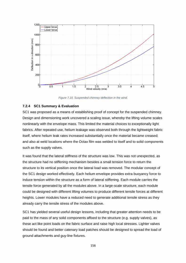
156
Figure 7.10. Suspended chimney deflection in the wind.
7.2.4 SC1 Summary & Evaluation
SC1 was proposed as a means of establishing proof of concept for the suspended chimney.
Design and dimensioning work uncovered a scaling issue, whereby the lifting volume scales
nonlinearly with the envelope mass. This limited the material choices to exceptionally light
fabrics. After repeated use, helium leakage was observed both through the lightweight fabric
itself, where helium leak rates increased substantially once the material became creased;
and also at weld locations where the Octax film was welded to itself and to solid components
such as the supply valves.
It was found that the lateral stiffness of the structure was low. This was not unexpected, as
the structure had no stiffening mechanism besides a small tension force to return the
structure to its vertical position once the lateral load was removed. The modular concept of
the SC1 design worked effectively. Each helium envelope provides extra buoyancy force to
induce tension within the structure as a form of lateral stiffening. Each module carries the
tensile force generated by all the modules above. In a large-scale structure, each module
could be designed with different lifting volumes to produce different tensile forces at different
heights. Lower modules have a reduced need to generate additional tensile stress as they
already carry the tensile stress of the modules above.
SC1 has yielded several useful design lessons, including that greater attention needs to be
paid to the mass of any solid components affixed to the structure (e.g. supply valves), as
these act like point loads on the fabric surface and raise high local stresses. Lighter valves
should be found and better catenary load patches should be designed to spread the load of
ground attachments and guy-line fixtures.

157
The use of helium raises several issues. At the desired scale, and to ensure the correct
slenderness ratio for a chimney structure, the helium volume was severely limited, reducing
the lifting force and necessitating the use of exceptionally light Octax fabric film.
Furthermore, some form of stiffening mechanism will be required to enable the structure to
withstand greater lateral loads, of the type it will encounter in real-world use. Such a
structure may involve the use of high-pressure air-inflated envelopes to provide lateral
stiffness while retaining the benefits of small stowed volume and low mass which
accompany inflated fabric structures. The second-generation prototype, SC2, will take these
design lessons forward and investigate the suspended chimney design with a stiffening
mechanism, at a similar laboratory scale.
7.3 SC2 PROTOTYPE
Following the experiments carried out with SC1, a novel design for the suspended chimney
was conceived whereby additional pressurised air-filled “sheathes” were included on the
inner and outer walls of the helium-filled lifting volume (see Figure 7.11). These sheathes,
pressurised with air, would have a greater lateral stiffness than the helium envelope,
providing resistance to wind loads. Additionally, while formers will be required within both
sheathes to maintain the structure’s shape, they will not be required within the helium
envelope, reducing the total mass to be lifted. This design also has axial symmetry, giving
the structure the same resistance to wind loading regardless of wind direction. It was
considered that this basic concept was worthy of further investigation and hence the design
was taken forward to be developed and manufactured as the SC2 suspended chimney
prototype.
Figure 7.11 shows a complete and cut-away example of the proposed suspended chimney
design, scaled to a prototype 20 m tall and with an internal flow diameter of 1 m. The outer
diameter is large compared to the “useful” flow diameter, at 8.34 m. The large outer diameter
is required to contain enough helium to lift the fabric mass. The real structure would not have
smooth sides, but would rather form ridges in between each of the formers within the
pressurised sheathes.

158
Figure 7.11. Suspended chimney using the proposed design, with thin high-pressure inner and outer sheathes. Chimney shown has been dimensioned for an internal flow diameter of 1.0 m and a height of 20.0 m in two
modules.
The following two suspended chimney prototypes (SC2 & SC3) are based on this design
concept (a helium volume enclosed by high-pressure air-filled sheathes). This chapter
presents the designs and assesses their ease of manufacture and any issues encountered
during their use, drawing out lessons for the design of future suspended chimney prototypes
and products. The experimental testing and analysis of the prototypes’ behaviour under load
is explored in Chapter 8.
7.3.1 SC2 Dimensioning
Dimensioning for any structure supported aloft by lighter-than-air gas will always present an
obstacle in that the mass to be supported by the lifting volume is defined in part by the
surface area of the lifting volume (the fabric envelope containing the lighter-than-air gas).
Thus finding the dimensions of the lifting volume is always a nonlinear problem. Fortunately
in the present design, the problem is quadratic and can be resolved with the solution of a
quadratic equation. This section will derive the quadratic equation which permits the user to
find the lifting volume dimensions for the SC2 suspended chimney design.
The general design of the SC2 prototype takes the form shown in Figure 7.12. Each module
is made from three nested tori, the outer two (labelled 1 and 3 in Figure 7.12) are thin high-
pressure tori which contain the central low-positive-pressure helium-filled volume and
provide structural stiffening. A succession of modules like that shown in Figure 7.12 can be

159
stacked and joined together to form a taller chimney structure, as shown in the 3D render in
Figure 7.11. The chimney void has diameter 2𝑟1.
Figure 7.12. SC2 concept diagram showing the key dimensions of one cell wall cross-section, enclosing an
internal flow area of radius r1.
As with all lighter-than-air structures, the lift is proportional to the lifting volume – in this case,
𝑉2 – while the mass is proportional to the fabric surface area plus some fixed (“dead”) mass
for air supply tubes and other pneumatic control equipment. In order to determine the mass
and the buoyancy force of a suspended chimney module of this design, a series of
parameters need to be defined as shown in Appendix IV.
The width of the helium cell is determined according to this quadratic equation in d2
2
2 2 2
2 3 3 3 3 2 1 2
1 1 1 3 3 3 3
1 1 2 1 1 3 3 3 1
)
2 ) (2 ) (2 )( )
( 2 ) ( 2
(2
(
)
( 4 2 2 2 )( ) 0x T
hd
h h d h d r
d rh d d h
m Fd h h
d
d d h hd r dg
(7.3)
where 1 1 a ; 2 2a ; and 3 3 a . Note that in this formulation the
order of the densities is reversed for the helium cell (subscript 2) to ensure that the
terms always remain positive. Equation (7.3) is derived in Appendix V. For the lighter-than-
air gas envelope, which contains a mixture of lighter-than-air gas (subscript g) and ambient
air (subscript ∞), 2 is calculated according to the Ideal Gas Law as

160
2
2 22 ,
11
g
p p
T R
p
R
(7.4)
where is the proportion (by volume) of the lifting volume filled by lighter-than-air gas.
Equation (7.3) is easily solved computationally, producing only one real positive result, which
is the helium cell width required to lift the specified suspended chimney module with
specified dead mass and tension.
A sensitivity analysis has been undertaken using the model described above to assess the
impact of different parameters upon dimensioning. All parameters other than those under
study are fixed at the reference values given in Appendix IV, and the total chimney height is
fixed at 20 m. Figure 7.13 shows how the total chimney diameter (important for maintaining a
suitable slenderness ratio) varies with the internal flow diameter specified in the design. The
relationship between flow diameter and external diameter is nearly linear. For larger
diameters, the wall thickness is almost constant. The wall thickness varies with diameter
only if an additional dead mass is included (the mx term in Equation (7.3)). The dead mass
accounts for pneumatic equipment, instrumentation and additional fabric for joints, and since
it is not assumed to scale linearly with fabric area, it will cause variations in wall thickness as
the internal flow diameter is changed.
Figure 7.13. Relationship between external (total) chimney diameter and internal chimney flow diameter for the SC2 design.
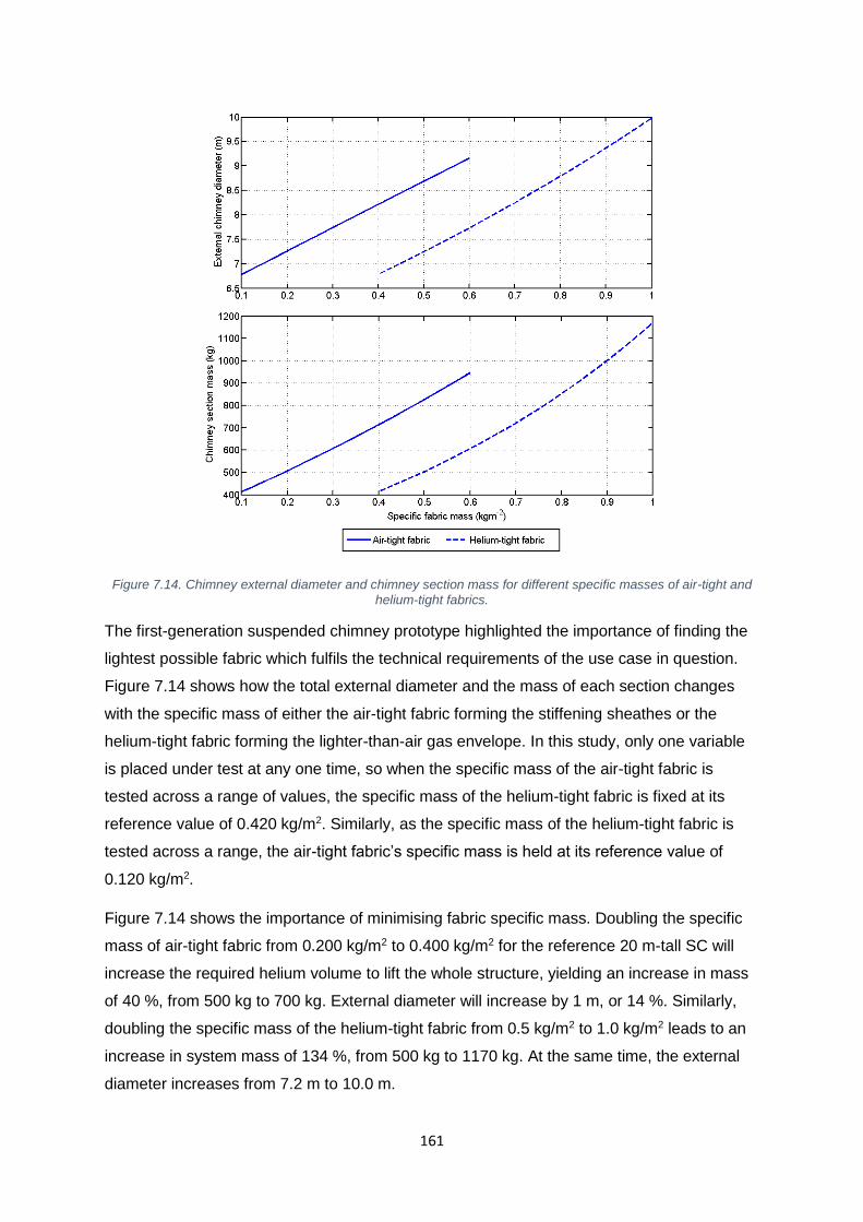
161
Figure 7.14. Chimney external diameter and chimney section mass for different specific masses of air-tight and
helium-tight fabrics.
The first-generation suspended chimney prototype highlighted the importance of finding the
lightest possible fabric which fulfils the technical requirements of the use case in question.
Figure 7.14 shows how the total external diameter and the mass of each section changes
with the specific mass of either the air-tight fabric forming the stiffening sheathes or the
helium-tight fabric forming the lighter-than-air gas envelope. In this study, only one variable
is placed under test at any one time, so when the specific mass of the air-tight fabric is
tested across a range of values, the specific mass of the helium-tight fabric is fixed at its
reference value of 0.420 kg/m2. Similarly, as the specific mass of the helium-tight fabric is
tested across a range, the air-tight fabric’s specific mass is held at its reference value of
0.120 kg/m2.
Figure 7.14 shows the importance of minimising fabric specific mass. Doubling the specific
mass of air-tight fabric from 0.200 kg/m2 to 0.400 kg/m2 for the reference 20 m-tall SC will
increase the required helium volume to lift the whole structure, yielding an increase in mass
of 40 %, from 500 kg to 700 kg. External diameter will increase by 1 m, or 14 %. Similarly,
doubling the specific mass of the helium-tight fabric from 0.5 kg/m2 to 1.0 kg/m2 leads to an
increase in system mass of 134 %, from 500 kg to 1170 kg. At the same time, the external
diameter increases from 7.2 m to 10.0 m.
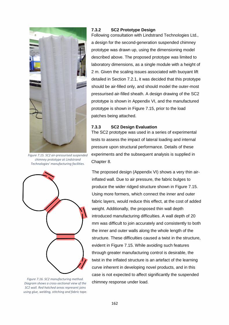
162
7.3.2 SC2 Prototype Design
Following consultation with Lindstrand Technologies Ltd.,
a design for the second-generation suspended chimney
prototype was drawn up, using the dimensioning model
described above. The proposed prototype was limited to
laboratory dimensions, as a single module with a height of
2 m. Given the scaling issues associated with buoyant lift
detailed in Section 7.2.1, it was decided that this prototype
should be air-filled only, and should model the outer-most
pressurised air-filled sheath. A design drawing of the SC2
prototype is shown in Appendix VI, and the manufactured
prototype is shown in Figure 7.15, prior to the load
patches being attached.
7.3.3 SC2 Design Evaluation
The SC2 prototype was used in a series of experimental
tests to assess the impact of lateral loading and internal
pressure upon structural performance. Details of these
experiments and the subsequent analysis is supplied in
Chapter 8.
The proposed design (Appendix VI) shows a very thin air-
inflated wall. Due to air pressure, the fabric bulges to
produce the wider ridged structure shown in Figure 7.15.
Using more formers, which connect the inner and outer
fabric layers, would reduce this effect, at the cost of added
weight. Additionally, the proposed thin wall depth
introduced manufacturing difficulties. A wall depth of 20
mm was difficult to join accurately and consistently to both
the inner and outer walls along the whole length of the
structure. These difficulties caused a twist in the structure,
evident in Figure 7.15. While avoiding such features
through greater manufacturing control is desirable, the
twist in the inflated structure is an artefact of the learning
curve inherent in developing novel products, and in this
case is not expected to affect significantly the suspended
chimney response under load.
Figure 7.15. SC2 air-pressurised suspended chimney prototype at Lindstrand
Technologies' manufacturing facilities.
Figure 7.16. SC2 manufacturing method. Diagram shows a cross-sectional view of the SC2 wall. Red hatched areas represent joins
using glue, welding, stitching and fabric tape.
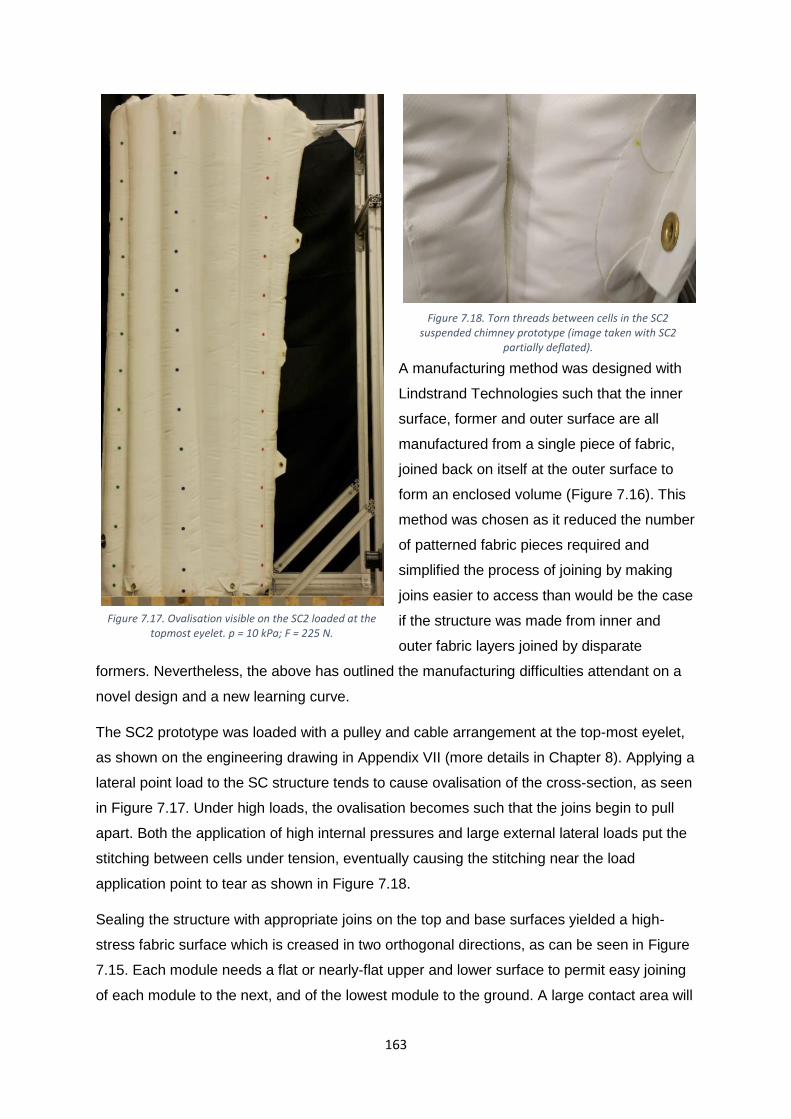
163
A manufacturing method was designed with
Lindstrand Technologies such that the inner
surface, former and outer surface are all
manufactured from a single piece of fabric,
joined back on itself at the outer surface to
form an enclosed volume (Figure 7.16). This
method was chosen as it reduced the number
of patterned fabric pieces required and
simplified the process of joining by making
joins easier to access than would be the case
if the structure was made from inner and
outer fabric layers joined by disparate
formers. Nevertheless, the above has outlined the manufacturing difficulties attendant on a
novel design and a new learning curve.
The SC2 prototype was loaded with a pulley and cable arrangement at the top-most eyelet,
as shown on the engineering drawing in Appendix VII (more details in Chapter 8). Applying a
lateral point load to the SC structure tends to cause ovalisation of the cross-section, as seen
in Figure 7.17. Under high loads, the ovalisation becomes such that the joins begin to pull
apart. Both the application of high internal pressures and large external lateral loads put the
stitching between cells under tension, eventually causing the stitching near the load
application point to tear as shown in Figure 7.18.
Sealing the structure with appropriate joins on the top and base surfaces yielded a high-
stress fabric surface which is creased in two orthogonal directions, as can be seen in Figure
7.15. Each module needs a flat or nearly-flat upper and lower surface to permit easy joining
of each module to the next, and of the lowest module to the ground. A large contact area will
Figure 7.17. Ovalisation visible on the SC2 loaded at the topmost eyelet. p = 10 kPa; F = 225 N.
Figure 7.18. Torn threads between cells in the SC2 suspended chimney prototype (image taken with SC2
partially deflated).
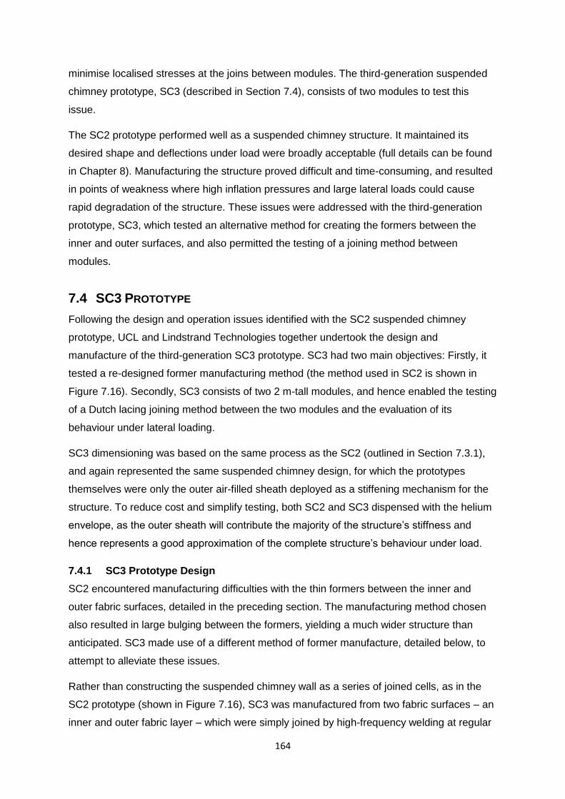
164
minimise localised stresses at the joins between modules. The third-generation suspended
chimney prototype, SC3 (described in Section 7.4), consists of two modules to test this
issue.
The SC2 prototype performed well as a suspended chimney structure. It maintained its
desired shape and deflections under load were broadly acceptable (full details can be found
in Chapter 8). Manufacturing the structure proved difficult and time-consuming, and resulted
in points of weakness where high inflation pressures and large lateral loads could cause
rapid degradation of the structure. These issues were addressed with the third-generation
prototype, SC3, which tested an alternative method for creating the formers between the
inner and outer surfaces, and also permitted the testing of a joining method between
modules.
7.4 SC3 PROTOTYPE
Following the design and operation issues identified with the SC2 suspended chimney
prototype, UCL and Lindstrand Technologies together undertook the design and
manufacture of the third-generation SC3 prototype. SC3 had two main objectives: Firstly, it
tested a re-designed former manufacturing method (the method used in SC2 is shown in
Figure 7.16). Secondly, SC3 consists of two 2 m-tall modules, and hence enabled the testing
of a Dutch lacing joining method between the two modules and the evaluation of its
behaviour under lateral loading.
SC3 dimensioning was based on the same process as the SC2 (outlined in Section 7.3.1),
and again represented the same suspended chimney design, for which the prototypes
themselves were only the outer air-filled sheath deployed as a stiffening mechanism for the
structure. To reduce cost and simplify testing, both SC2 and SC3 dispensed with the helium
envelope, as the outer sheath will contribute the majority of the structure’s stiffness and
hence represents a good approximation of the complete structure’s behaviour under load.
7.4.1 SC3 Prototype Design
SC2 encountered manufacturing difficulties with the thin formers between the inner and
outer fabric surfaces, detailed in the preceding section. The manufacturing method chosen
also resulted in large bulging between the formers, yielding a much wider structure than
anticipated. SC3 made use of a different method of former manufacture, detailed below, to
attempt to alleviate these issues.
Rather than constructing the suspended chimney wall as a series of joined cells, as in the
SC2 prototype (shown in Figure 7.16), SC3 was manufactured from two fabric surfaces – an
inner and outer fabric layer – which were simply joined by high-frequency welding at regular
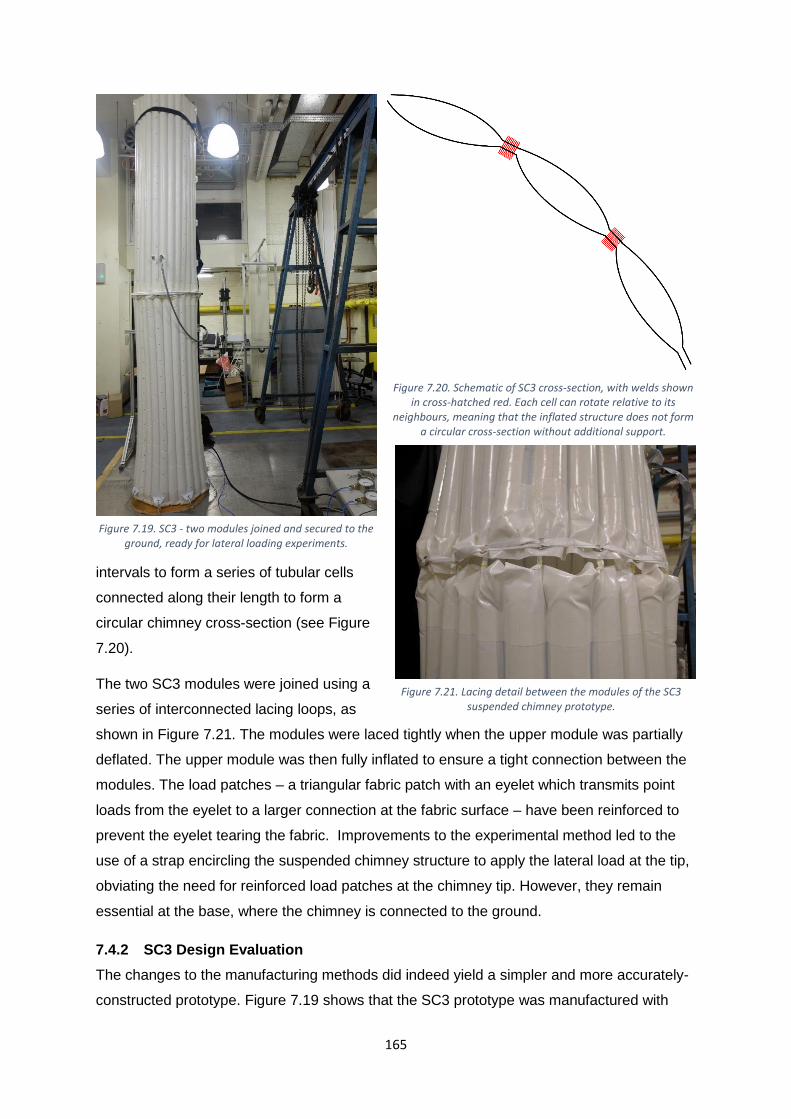
165
intervals to form a series of tubular cells
connected along their length to form a
circular chimney cross-section (see Figure
7.20).
The two SC3 modules were joined using a
series of interconnected lacing loops, as
shown in Figure 7.21. The modules were laced tightly when the upper module was partially
deflated. The upper module was then fully inflated to ensure a tight connection between the
modules. The load patches – a triangular fabric patch with an eyelet which transmits point
loads from the eyelet to a larger connection at the fabric surface – have been reinforced to
prevent the eyelet tearing the fabric. Improvements to the experimental method led to the
use of a strap encircling the suspended chimney structure to apply the lateral load at the tip,
obviating the need for reinforced load patches at the chimney tip. However, they remain
essential at the base, where the chimney is connected to the ground.
7.4.2 SC3 Design Evaluation
The changes to the manufacturing methods did indeed yield a simpler and more accurately-
constructed prototype. Figure 7.19 shows that the SC3 prototype was manufactured with
Figure 7.19. SC3 - two modules joined and secured to the ground, ready for lateral loading experiments.
Figure 7.21. Lacing detail between the modules of the SC3 suspended chimney prototype.
Figure 7.20. Schematic of SC3 cross-section, with welds shown in cross-hatched red. Each cell can rotate relative to its
neighbours, meaning that the inflated structure does not form a circular cross-section without additional support.

166
straight equally-spaced formers. The
simpler design meant that more formers
could be used without increasing
manufacturing time or expense, leading to
a thinner pressurised wall more aligned to
the envisioned design.
However, the new former design removed
a constraint on the movement of one cell
relative to another – each cell could rotate
around the welded joints on either side of
it. In terms of the whole prototype
structure, this meant there was nothing to
maintain the structure in a circular cross-
section. SC2 naturally formed a circular
cross-section when inflated, but SC3 did
not form that shape unless supported by
ground connections or internal
reinforcements. While SC3 solved some
issues identified with the SC2 prototype, a
new issue of the circular cross-section was
introduced, which had implications for bending stiffness, as the SC3 cross section is more
likely to collapse under load.
The lacing joining the two SC3 modules secured the two modules together, but it proved not
to be sufficiently tight or strong under large tip loads, leading to the modules separating and
the join between the modules operating as a stiff hinge (see Figure 7.22). The connection to
the ground proved similarly difficult to secure without a degree of rotation. Figure 7.22 also
shows the collapse of the cross-sectional shape at the join (ovalisation with the narrow side
face-on to the camera) and at the tip (ovalisation with the wide side face-on). The cross-
sectional shape was maintained in part by the ground connectors imposing radial outward
tension which stretched the base, as well as securing the structure vertically. A broader base
contributed to the stability of the structure by supplying a greater second moment of area
where the bending moment carried by the structure is greatest.
Given the issues encountered with module connections and with maintaining the structure’s
cross-sectional shape, a series of flexible plastic hoops were installed within the structure
and at the laced connection between the modules to promote more beam-like behaviour.
Figure 7.22. Both modules of the SC3 prototype loaded at the tip, demonstrating the action of the laced joint as a stiff hinge.
p = 30 kPa; F = 172 N.

167
Three were installed within each module and an additional hoop was installed at the
modules’ laced connection (Figure 7.24a). A wooden platform was installed between the
structure and its ground connections to increase the distance between the eyelets and the
ground, enabling a greater vertical tensile stress to be induced in the fabric, ensuring a
better connection to the ground (Figure 7.24b). These design changes stiffened the SC3
prototype, as can be seen in Figure 7.23.
7.5 SC4 PROTOTYPE The SC3 prototype highlighted a few issues which remain to be resolved. Specifically, the
new method of manufacturing formers used for SC3 proved to be quicker, as anticipated, but
resulted in problems maintaining the prototype’s circular cross section. Additionally, the
lacing design of SC3 was not sufficiently tight to make the structure perform as a single
continuous beam. Before larger structures can be built, these issues need to be resolved. A
further two modules, of the same dimensions have therefore been commissioned from
Lindstrand Technologies. This prototype, SC4, has now been built and is awaiting testing at
Figure 7.24. SC3 strengthening modifications. (a) plastic hoops to strengthen the joint between the
modules; and (b) a wooden platform installed to raise the base of the fabric and increase the tension applied
to secure the structure.
Figure 7.23. SC3 prototype with cross-sectional reinforcement (plastic hoops), joint reinforcement and base reinforcement.
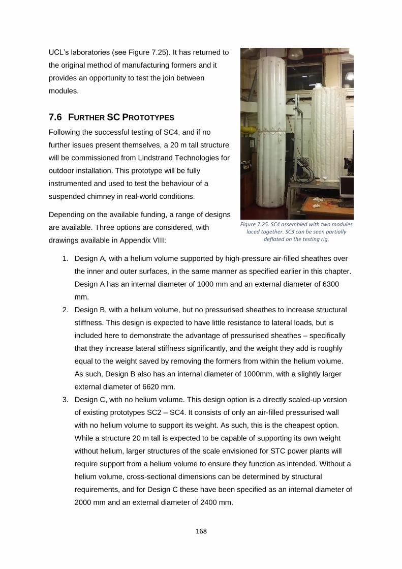
168
UCL’s laboratories (see Figure 7.25). It has returned to
the original method of manufacturing formers and it
provides an opportunity to test the join between
modules.
7.6 FURTHER SC PROTOTYPES
Following the successful testing of SC4, and if no
further issues present themselves, a 20 m tall structure
will be commissioned from Lindstrand Technologies for
outdoor installation. This prototype will be fully
instrumented and used to test the behaviour of a
suspended chimney in real-world conditions.
Depending on the available funding, a range of designs
are available. Three options are considered, with
drawings available in Appendix VIII:
1. Design A, with a helium volume supported by high-pressure air-filled sheathes over
the inner and outer surfaces, in the same manner as specified earlier in this chapter.
Design A has an internal diameter of 1000 mm and an external diameter of 6300
mm.
2. Design B, with a helium volume, but no pressurised sheathes to increase structural
stiffness. This design is expected to have little resistance to lateral loads, but is
included here to demonstrate the advantage of pressurised sheathes – specifically
that they increase lateral stiffness significantly, and the weight they add is roughly
equal to the weight saved by removing the formers from within the helium volume.
As such, Design B also has an internal diameter of 1000mm, with a slightly larger
external diameter of 6620 mm.
3. Design C, with no helium volume. This design option is a directly scaled-up version
of existing prototypes SC2 – SC4. It consists of only an air-filled pressurised wall
with no helium volume to support its weight. As such, this is the cheapest option.
While a structure 20 m tall is expected to be capable of supporting its own weight
without helium, larger structures of the scale envisioned for STC power plants will
require support from a helium volume to ensure they function as intended. Without a
helium volume, cross-sectional dimensions can be determined by structural
requirements, and for Design C these have been specified as an internal diameter of
2000 mm and an external diameter of 2400 mm.
Figure 7.25. SC4 assembled with two modules laced together. SC3 can be seen partially
deflated on the testing rig.

169
All three design options are presented in technical drawings in Appendix VIII. In brief, Design
A – expected to have the greatest lateral stiffness, and be the closest to the eventual SC
product – is expected to cost about $67k to manufacture and test. A rendered image of this
design is shown in Figure 7.11 earlier in the chapter. Design C, which is a scaled version of
existing prototypes, is expected to cost $19,000 to manufacture and test. Figure 7.26 and
Figure 7.27 show the breakdown of these costs, with labour costs dominating in both.
Helium supply and the associated equipment accounts for 10 % of the cost of Design A, or
$6,800.
Using the method outlined in Appendix V, a suspended chimney 100 m tall is specified and
costed. It has an internal flow diameter of 5 m and is built from five modules, each 20 m tall,
using Design A which includes a helium lifting volume and pressurised sheathes. The 100 m
tall SC is forecast to cost $364,000 to the first full inflation (i.e. excluding future deflations
and inflations and helium top-ups). Of this, $84,000 is spent on fabric materials, $241,000 is
spent on labour, and helium is expected to cost $39,000.
Figure 7.26. Design A cost breakdown - 20 m tall helium-supported SC with pressurised air-filled sheathes for lateral stiffness.
Fabric & materials,
$17,832 , 27%
Lacing / joining, $922 , 1%
Pneumatics, $670 , 1%
He gas (single inflation), $5,326 , 8%
He equipment (6-month hire), $804 , 1%Instrumentation, $2,680 , 4%
Labour, $38,253 , 57%
Shipping, $402 , 1%

170
Figure 7.27. Design C cost breakdown - 20 m tall SC consisting of an air-filled wall only.
7.7 CONCLUSIONS
This chapter has introduced the first three suspended chimney prototypes, manufactured by
Lindstrand Technologies Ltd. and tested at UCL’s laboratories. These prototypes are the first
practical investigations working towards commercial-scale suspended chimneys of 50 m or
taller. A fourth prototype has been manufactured, and is awaiting testing. Larger commercial-
scale SCs are described.
The first prototype, SC1, was a helium-supported proof-of-concept prototype which required
the use of exceptionally lightweight helium-tight film. Reducing the SC prototype to a size
suitable for laboratory use (SC1 was 3.5 m tall) uncovered scaling issues whereby the lifting
volume scales nonlinearly with the envelope area, which defines the mass to be lifted. SC1
was capable of supporting its own weight and additional lifting volume was specified to
produce a small tensile force which kept the structure in an upright position and provided
some resistance to lateral loads. Under testing, it was shown that this lateral stiffness is
minimal and that dedicated stiffening mechanisms will be essential for larger structures
required to withstand real-world loading. The lightweight fabric film proved to be not
sufficiently durable, and helium leak rates increased substantially following a few cycles of
inflation and deflation. While the SC1 prototype was able to support its own weight, the
issues of scaling, weight carrying capability, and lateral stiffening severely limited its real-
world utility.
Fabric & materials, $5,456 , 29%
Lacing / joining, $909 , 5%
Pneumatics, $670 , 4%
Instrumentation, $2,680 , 14%
Labour, $8,669 , 46%
Shipping, $402 , 2%

171
The second-generation suspended chimney prototype, SC2, was created to address these
issues. After investigating various designs, it was decided that a double-skinned wall
consisting of high-pressure air-filled sheathes on the inner and outer surfaces of a void filled
with helium would enable the structure to provide the greatest lift per unit height, reducing
the overall diameter. The high internal pressure provides a stiffening mechanism with axial
symmetry. Rather than construct a scaled version of the whole suspended chimney, a
scaled air-pressurised outer sheath was proposed. Under high internal pressure and large
lateral loads, some tearing of the stitching and load patches was observed. Despite these
issues, the SC2 structure operated well and resisted substantial lateral loads. It was inflated
successfully up to 50 kPa and survived multiple inflations and deflations without a noticeable
degradation in performance.
A third-generation suspended chimney prototype, SC3, was manufactured. Based on the
same design and dimensions as SC2, changes were made to the quantity of formers and
their method of manufacture, aiming to simplify the process and produce a thinner wall. This
change in design had the unintended consequence of introducing an additional degree of
freedom to the structure’s walls, such that each air-filled “cell” could rotate about the welds
either side of it. As a result, the SC3 required circular plastic hoops and strong ground
connections to ensure that the cross-section did not collapse. SC3 consisted of two 2 m-tall
modules joined with lacing, which proved too loose, causing the joint to act as a hinge. More
plastic hoops were used to strengthen the joint.
The experience of designing and manufacturing three suspended chimney prototypes has
provided a greater degree of confidence that the proposed design is a reasonable solution to
the problems of weight – which must be minimised – and lateral stiffness – which must be
maximised. The sheathes both constrain the helium envelope and provide lateral stiffness.
The formers within the sheathes must consist of a length (as in SC2) and not a point (as in
SC3), otherwise the structure loses its coherence in cross-section. The join between
modules must be sufficiently strong to transmit the bending loads without acting as a hinge.
7.7.1 Future Work
A further 4 m tall prototype, SC4, has been manufactured and is awaiting testing at UCL. If
the issues of joint weakness and cross-sectional coherence have been resolved, a larger SC
(up to 20 m tall) will be built. Dimensions and cost forecasts are given in Chapter 9.
Besides building larger prototypes, material properties remains an important area of future
work. Currently, SC2 and SC3 use materials which Lindstrand Technologies has tested
extensively for use in their commercial products. The suspended chimney represents a
different use case which may require further testing to establish material behaviour. Material

172
durability under repeated flexure remains to be assessed, as does material performance
under high-UV (high-insolation) conditions and dynamic weather loads. Large-scale
commercial SCs will most likely require a level of automated manufacture to ensure
commercial viability. Automated manufacturing methods are not currently highly developed
for fabric structures.
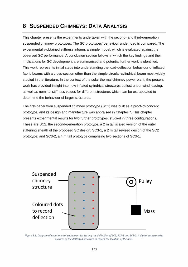
173
8 SUSPENDED CHIMNEYS: DATA ANALYSIS
This chapter presents the experiments undertaken with the second- and third-generation
suspended chimney prototypes. The SC prototypes’ behaviour under load is compared. The
experimentally-obtained stiffness informs a simple model, which is evaluated against the
observed SC performance. A conclusion section follows in which the key findings and their
implications for SC development are summarised and potential further work is identified.
This work represents initial steps into understanding the load-deflection behaviour of inflated
fabric beams with a cross-section other than the simple circular-cylindrical beam most widely
studied in the literature. In the context of the solar thermal chimney power plant, the present
work has provided insight into how inflated cylindrical structures deflect under wind loading,
as well as nominal stiffness values for different structures which can be extrapolated to
determine the behaviour of larger structures.
The first-generation suspended chimney prototype (SC1) was built as a proof-of-concept
prototype, and its design and manufacture was appraised in Chapter 7. This chapter
presents experimental results for two further prototypes, studied in three configurations.
These are SC2, the second-generation prototype, a 2 m tall scaled version of the outer
stiffening sheath of the proposed SC design; SC3-1, a 2 m tall revised design of the SC2
prototype; and SC3-2, a 4 m tall prototype comprising two sections of SC3-1.
Figure 8.1. Diagram of experimental equipment for testing the deflection of SC2, SC3-1 and SC3-2. A digital camera takes pictures of the deflected structure to record the location of the dots.

174
8.1 EXPERIMENTAL METHOD The suspended chimneys require a
quantified experimental process to assess
their performance and develop improved
designs. The bending stiffness of inflated
structures is typically less than that of
conventional structural systems, and the
suspended chimney’s ability to withstand
significant wind loads must be assessed. To
that end, an experimental method has been
devised which aims to measure lateral
stiffness through a load-deflection analysis,
identify the onset of wrinkling under different
load and pressure conditions, and use this
data to assess the accuracy of a simple
beam-bending model. Throughout these
experiments, the beam was tip-loaded with a
built-in connection at the base.
8.1.1 Securing and Loading the
Prototypes
The experimental method is similar for all
prototypes, and is shown diagrammatically
in Figure 8.1. The suspended chimney
structure is inflated to a prescribed
pressure and secured at the base with
turnbuckles, which can be tightened to
stiffen the connection to the ground and
prevent translation or rotation of the base.
A small wooden platform, visible in Figure
8.2, is used to raise the base of the SC
prototypes by 30 mm, enabling a greater tension - and therefore a more secure connection -
to be achieved with the turnbuckles. A pulley system loads the chimney laterally at the tip
with a fixed load. A belt is wrapped around the structure at the load height to spread the
lateral load around the cross-section and limit the deformation of the structure. Cross-
sectional deformation at the prototypes’ free end would be more severe if the loading pulley
were attached directly to one side of the structure.
Image resolution 16 megapixels, 4896 x
3264 pixels.
Image format JPG
Trigger mechanism Remote, via WiFi.
Focal length 16 mm
Aperture f/3.5
Shutter speed 1/40 sec.
Flash mode Disabled
Figure 8.2. SC2 with coloured dots for deflection tracking, loaded with a loop wrapped around the tip. P = 40 kPa; F =
323 N. SC3-1 can be seen in the background awaiting testing.
Table 8.1. FujiFilm X-T10 camera properties.
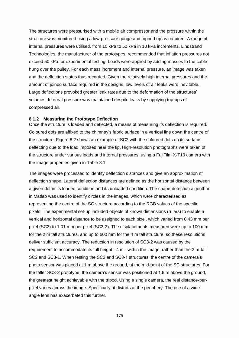
175
The structures were pressurised with a mobile air compressor and the pressure within the
structure was monitored using a low-pressure gauge and topped up as required. A range of
internal pressures were utilised, from 10 kPa to 50 kPa in 10 kPa increments. Lindstrand
Technologies, the manufacturer of the prototypes, recommended that inflation pressures not
exceed 50 kPa for experimental testing. Loads were applied by adding masses to the cable
hung over the pulley. For each mass increment and internal pressure, an image was taken
and the deflection states thus recorded. Given the relatively high internal pressures and the
amount of joined surface required in the designs, low levels of air leaks were inevitable.
Large deflections provoked greater leak rates due to the deformation of the structures’
volumes. Internal pressure was maintained despite leaks by supplying top-ups of
compressed air.
8.1.2 Measuring the Prototype Deflection
Once the structure is loaded and deflected, a means of measuring its deflection is required.
Coloured dots are affixed to the chimney’s fabric surface in a vertical line down the centre of
the structure. Figure 8.2 shows an example of SC2 with the coloured dots on its surface,
deflecting due to the load imposed near the tip. High-resolution photographs were taken of
the structure under various loads and internal pressures, using a FujiFilm X-T10 camera with
the image properties given in Table 8.1.
The images were processed to identify deflection distances and give an approximation of
deflection shape. Lateral deflection distances are defined as the horizontal distance between
a given dot in its loaded condition and its unloaded condition. The shape-detection algorithm
in Matlab was used to identify circles in the images, which were characterised as
representing the centre of the SC structure according to the RGB values of the specific
pixels. The experimental set-up included objects of known dimensions (rulers) to enable a
vertical and horizontal distance to be assigned to each pixel, which varied from 0.43 mm per
pixel (SC2) to 1.01 mm per pixel (SC3-2). The displacements measured were up to 100 mm
for the 2 m tall structures, and up to 600 mm for the 4 m tall structure, so these resolutions
deliver sufficient accuracy. The reduction in resolution of SC3-2 was caused by the
requirement to accommodate its full height - 4 m - within the image, rather than the 2 m-tall
SC2 and SC3-1. When testing the SC2 and SC3-1 structures, the centre of the camera’s
photo sensor was placed at 1 m above the ground, at the mid-point of the SC structures. For
the taller SC3-2 prototype, the camera’s sensor was positioned at 1.8 m above the ground,
the greatest height achievable with the tripod. Using a single camera, the real distance-per-
pixel varies across the image. Specifically, it distorts at the periphery. The use of a wide-
angle lens has exacerbated this further.

176
8.1.3 Obtaining Bending Stiffness and Creating a Simple Bending Model
The deflection data obtained from the images was processed to obtain a nominal bending
stiffness for each structure and variation of internal pressure. This was done by treating the
inflated prototypes as Euler-Bernoulli beams and using the known loads and observed
deflections to calculate bending stiffness. From a review of the literature, it is known that
internal pressure affects stiffness and that the Euler-Bernoulli beam model is considered
insufficient as it neglects shear stresses, which are not negligibly small for inflatable beams.
This analysis makes use of the Euler-Bernoulli beam model, but with experimentally-
obtained bending stiffnesses, and in this way includes pressure effects.
As such, the Euler-Bernoulli bending stiffness of each prototype is calculated for each
pressure level according to
3
3,
FHEI
x (8.1)
where EI is the bending stiffness; F is the applied load; H is the height on the structure at
which the load is applied; and x is the deflection of the neutral axis at the point the load is
applied. The pressure is not modelled explicitly within this equation, but its effect is captured
by means of the different deflections (x) measured at each internal pressure level. The
calculated bending stiffnesses were then used to simulate the prototype’s deflection shape
as if it were an Euler-Bernoulli beam. In this way, the accuracy of the Euler-Bernoulli model
with experimentally-obtained bending stiffness values has been assessed.
8.1.4 Future Improvements to the Experimental Method
This experimental method has yielded useful data which is analysed in the remainder of this
chapter. However, it is worth appraising this method to identify improvements which could be
made in future similar experiments.
The camera was of a sufficiently high resolution for the image processing algorithm to be
able to identify the dots on the structures’ surfaces. However, this only yields positions data
at discrete points. More comprehensive image processing options exist, including digital
image correlation, which has previously been used by Clapp et al. [150] to study the
deflection of inflated circular-cylindrical beams. Such an approach would yield
comprehensive information regarding the stress and strain fields across the whole fabric
surface, enabling much more in-depth analysis of performance of the suspended chimney
prototypes.
At large deflections, the angle between the cable supplying the load and the horizontal
changes considerably. This angle increases due to the fixed height of the cable pulley
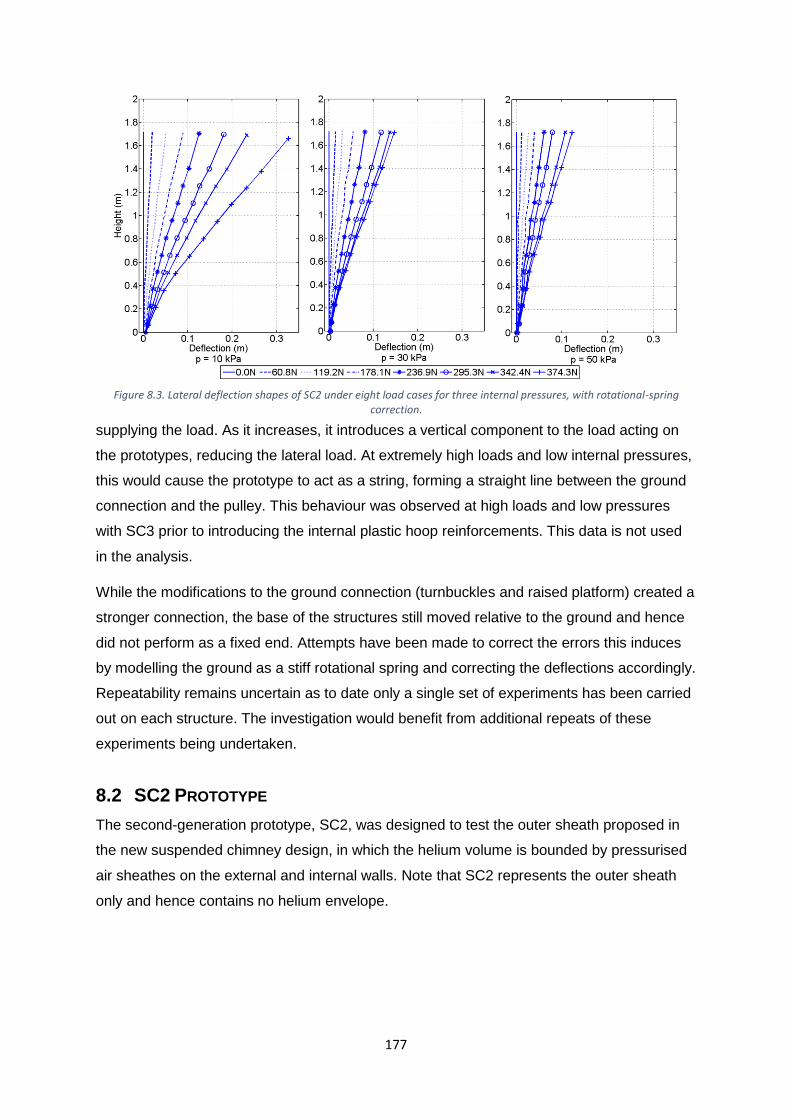
177
supplying the load. As it increases, it introduces a vertical component to the load acting on
the prototypes, reducing the lateral load. At extremely high loads and low internal pressures,
this would cause the prototype to act as a string, forming a straight line between the ground
connection and the pulley. This behaviour was observed at high loads and low pressures
with SC3 prior to introducing the internal plastic hoop reinforcements. This data is not used
in the analysis.
While the modifications to the ground connection (turnbuckles and raised platform) created a
stronger connection, the base of the structures still moved relative to the ground and hence
did not perform as a fixed end. Attempts have been made to correct the errors this induces
by modelling the ground as a stiff rotational spring and correcting the deflections accordingly.
Repeatability remains uncertain as to date only a single set of experiments has been carried
out on each structure. The investigation would benefit from additional repeats of these
experiments being undertaken.
8.2 SC2 PROTOTYPE
The second-generation prototype, SC2, was designed to test the outer sheath proposed in
the new suspended chimney design, in which the helium volume is bounded by pressurised
air sheathes on the external and internal walls. Note that SC2 represents the outer sheath
only and hence contains no helium envelope.
Figure 8.3. Lateral deflection shapes of SC2 under eight load cases for three internal pressures, with rotational-spring correction.

178
The deflection shapes of SC2 are given in Figure 8.3 for a range of internal pressures and
lateral tip loads. Efforts to secure the base as a fixed end were not completely successful
and as such Figure 8.3 incorporates a correction for lateral deflection which treats the base
as a stiff rotational spring, with the spring constant determined by the gradient of the position
of the lowest three dots. The deflection of the dots is corrected accordingly. Increasing load
increases the deflection of the structure, as would be expected. For a given load, increasing
internal pressure is shown to reduce deflection, an effect which is most pronounced at higher
loads. For example, under a lateral load of 342 N, the tip deflection reduces from 0.23 m at
10 kPa to 0.11 m at 50 kPa. At 10 kPa, there is a significantly larger tip deflection between
342 N and 374 N lateral load than is observed for either 30 kPa or 50 kPa. This is because
the structure has wrinkled (see Figure 8.4), and bending stiffness is significantly reduced for
inflated structures in the wrinkled state. For the same loads at 30 kPa and 50 kPa, the
change in deflection is very small due to the returning force which the internal pressure
imposes. For the SC2 at 10 kPa, wrinkling begins at approximately 250 N. For higher
internal pressures, wrinkling initiates at 260 – 330 N. Figure 8.3 indicates that low internal
pressures will most likely prove unsuitable for commercial SC products due to the high tip
deflection values and low bending stiffness.
The maximum deflection of the structure is of interest for analysing the structural
performance. Figure 8.5 shows the deflection of the tip of the structure under different loads
and internal pressures. It shows roughly linear
behaviour for all internal pressures, up to
approximately 150 N load. SC2 with 10 kPa internal
pressure demonstrates a higher lateral tip deflection
than other pressures; while 20 kPa – 50 kPa show
very similar deflections at low loads. Beyond 150 N
lateral load, there is a greater range of deflections
across different inflation pressures, although the
deflections at 40 kPa and 50 kPa internal pressure
continue to be similar across the entire range of lateral
loads tested. Beyond 150 N, the tip of SC2 inflated to
10 kPa begins to deflect non-linearly with load, as the
structure passes the onset of wrinkling. Higher
pressures continue to behave approximately linearly,
albeit with an increased load-deflection gradient. The
bending stiffness of SC2 is calculated using Equation
Figure 8.4. Wrinkling evident in the SC2 at 10 kPa loaded with 374 N.
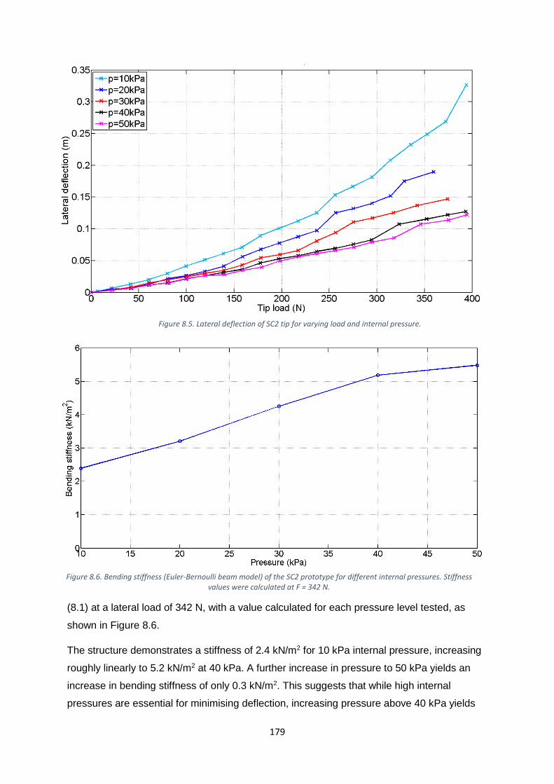
179
(8.1) at a lateral load of 342 N, with a value calculated for each pressure level tested, as
shown in Figure 8.6.
The structure demonstrates a stiffness of 2.4 kN/m2 for 10 kPa internal pressure, increasing
roughly linearly to 5.2 kN/m2 at 40 kPa. A further increase in pressure to 50 kPa yields an
increase in bending stiffness of only 0.3 kN/m2. This suggests that while high internal
pressures are essential for minimising deflection, increasing pressure above 40 kPa yields
Figure 8.5. Lateral deflection of SC2 tip for varying load and internal pressure.
Figure 8.6. Bending stiffness (Euler-Bernoulli beam model) of the SC2 prototype for different internal pressures. Stiffness values were calculated at F = 342 N.
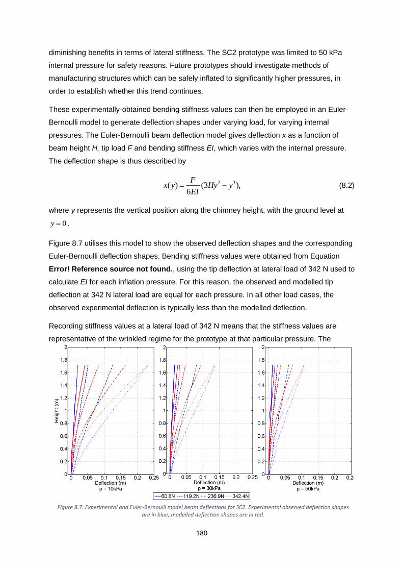
180
diminishing benefits in terms of lateral stiffness. The SC2 prototype was limited to 50 kPa
internal pressure for safety reasons. Future prototypes should investigate methods of
manufacturing structures which can be safely inflated to significantly higher pressures, in
order to establish whether this trend continues.
These experimentally-obtained bending stiffness values can then be employed in an Euler-
Bernoulli model to generate deflection shapes under varying load, for varying internal
pressures. The Euler-Bernoulli beam deflection model gives deflection x as a function of
beam height H, tip load F and bending stiffness EI, which varies with the internal pressure.
The deflection shape is thus described by
2 3(3 ,) )
6(
FHx yy
Ey
I (8.2)
where y represents the vertical position along the chimney height, with the ground level at
0y .
Figure 8.7 utilises this model to show the observed deflection shapes and the corresponding
Euler-Bernoulli deflection shapes. Bending stiffness values were obtained from Equation
Error! Reference source not found., using the tip deflection at lateral load of 342 N used to
calculate EI for each inflation pressure. For this reason, the observed and modelled tip
deflection at 342 N lateral load are equal for each pressure. In all other load cases, the
observed experimental deflection is typically less than the modelled deflection.
Recording stiffness values at a lateral load of 342 N means that the stiffness values are
representative of the wrinkled regime for the prototype at that particular pressure. The
Figure 8.7. Experimental and Euler-Bernoulli model beam deflections for SC2. Experimental observed deflection shapes are in blue, modelled deflection shapes are in red.

181
measured maximum (tip) deflection for each pressure does not increase linearly with load,
and does not match the Euler-Bernoulli beam. The observed deflection shapes at each load
and pressure are approximately linear, except with a kink near the base, where wrinkling has
occurred. This is in contrast to the Euler-Bernoulli beam deflection model, which predicts a
cubic deformation shape with height (Equation (8.2)). At approximately 240 N, the modelled
deflection is 31 % greater than the observed deflection for 10 kPa internal pressure (0.039 m
difference), and 20 % greater (0.012 m) for 50 kPa internal pressure, demonstrating that a
more comprehensive model has scope to improve upon the accuracy of simulations. Various
researchers writing about the simulation of inflatable beams have specified modified
Timoshenko beam theory to account for the non-negligible shear in inflatable structures
under load [133], [151].
Timoshenko beam theory would enable improved correlation between experimental
observations and model predictions compared to the Euler-Bernoulli beam theory utilised to
produce Figure 8.7. However, throughout the literature surveyed in Chapter 6, Timoshenko
beam theory was modified to include pressure as a follower force dependent on the beam
deflection shape, and such a model would be required to reduce discrepancies substantially.
Furthermore, wrinkling is not modelled in the present analysis, so wrinkled beam states,
under which increased deflection is normally observed, are not captured by the model.
The greatest tip load tested for the SC2 structure was 394 N, equivalent to a wind speed of
18.5 ms-1 acting across the whole height of the structure (assuming a drag coefficient of
1.17). For SC2 inflated to 50 kPa, this generated a tip deflection of 0.12 m. Tip loads are a
worst-case approximation of the real-world wind load distribution across the structure’s
surface. A load of 394 N is equivalent to a gale force 8 wind, and the relatively small
resulting deflection suggests that the current SC design could withstand significant wind
speeds.
8.3 SC3-1 PROTOTYPE
The SC2 prototype successfully resisted a lateral load with reasonable deflection. However,
taller structures would require multiple modules, and the means of joining these modules
represents an unknown variable which must be investigated before larger structures can be
deployed. For these reasons, the SC3 prototype was commissioned from Lindstrand
Technologies Ltd. A full description of the design of SC3 is given in Chapter 7, including
design changes compared to the SC2 prototype. This section presents the experimental
data and subsequent analysis for the SC3-1 prototype, that is: the 2 m-tall single module of
the third-generation suspended chimney prototype.
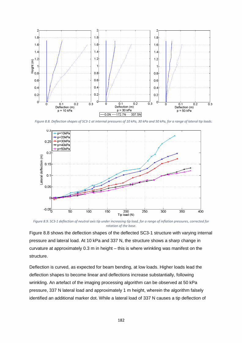
182
Figure 8.8 shows the deflection shapes of the deflected SC3-1 structure with varying internal
pressure and lateral load. At 10 kPa and 337 N, the structure shows a sharp change in
curvature at approximately 0.3 m in height – this is where wrinkling was manifest on the
structure.
Deflection is curved, as expected for beam bending, at low loads. Higher loads lead the
deflection shapes to become linear and deflections increase substantially, following
wrinkling. An artefact of the imaging processing algorithm can be observed at 50 kPa
pressure, 337 N lateral load and approximately 1 m height, wherein the algorithm falsely
identified an additional marker dot. While a lateral load of 337 N causes a tip deflection of
Figure 8.9. SC3-1 deflection of neutral axis tip under increasing tip load, for a range of inflation pressures, corrected for rotation of the base.
Figure 8.8. Deflection shapes of SC3-1 at internal pressures of 10 kPa, 30 kPa and 50 kPa, for a range of lateral tip loads.
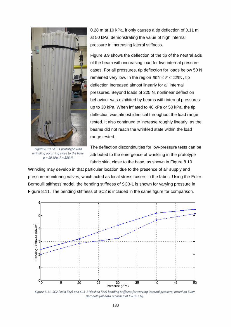
183
0.28 m at 10 kPa, it only causes a tip deflection of 0.11 m
at 50 kPa, demonstrating the value of high internal
pressure in increasing lateral stiffness.
Figure 8.9 shows the deflection of the tip of the neutral axis
of the beam with increasing load for five internal pressure
cases. For all pressures, tip deflection for loads below 50 N
remained very low. In the region 20N 5N5 2F , tip
deflection increased almost linearly for all internal
pressures. Beyond loads of 225 N, nonlinear deflection
behaviour was exhibited by beams with internal pressures
up to 30 kPa. When inflated to 40 kPa or 50 kPa, the tip
deflection was almost identical throughout the load range
tested. It also continued to increase roughly linearly, as the
beams did not reach the wrinkled state within the load
range tested.
The deflection discontinuities for low-pressure tests can be
attributed to the emergence of wrinkling in the prototype
fabric skin, close to the base, as shown in Figure 8.10.
Wrinkling may develop in that particular location due to the presence of air supply and
pressure monitoring valves, which acted as local stress raisers in the fabric. Using the Euler-
Bernoulli stiffness model, the bending stiffness of SC3-1 is shown for varying pressure in
Figure 8.11. The bending stiffness of SC2 is included in the same figure for comparison.
Figure 8.10. SC3-1 prototype with wrinkling occurring close to the base.
p = 10 kPa, F = 238 N.
Figure 8.11. SC2 (solid line) and SC3-1 (dashed line) bending stiffness for varying internal pressure, based on Euler Bernoulli (all data recorded at F = 337 N).
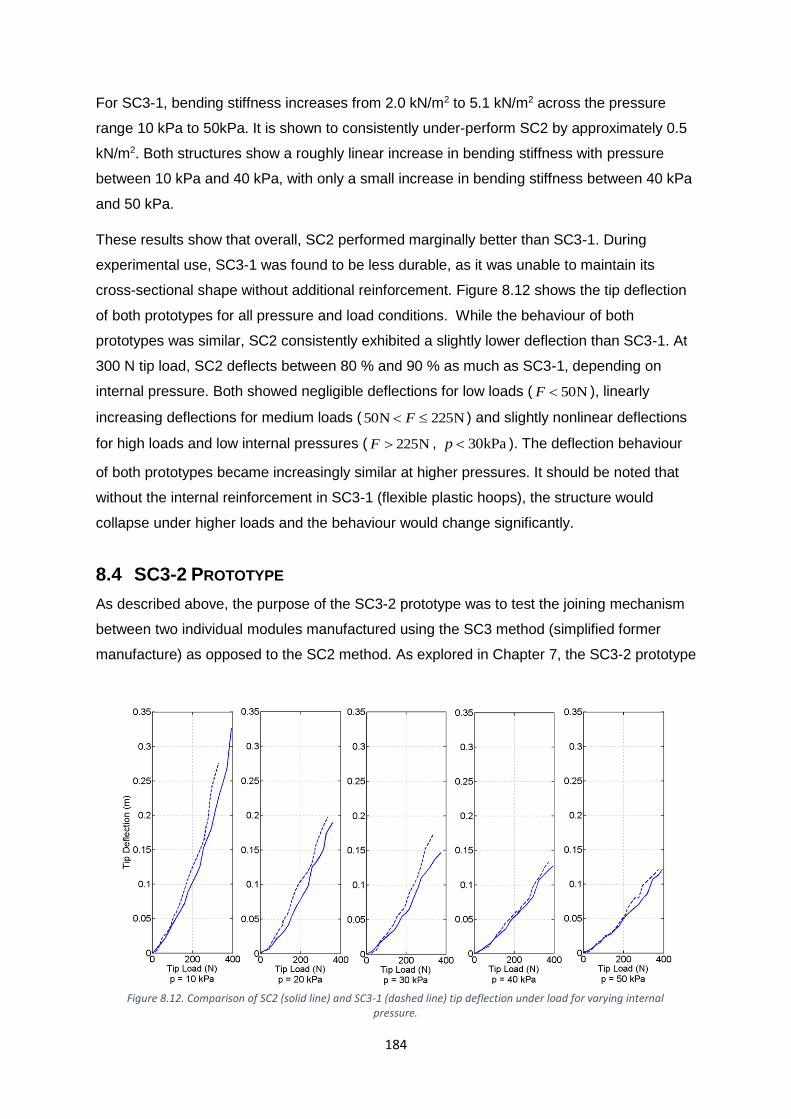
184
For SC3-1, bending stiffness increases from 2.0 kN/m2 to 5.1 kN/m2 across the pressure
range 10 kPa to 50kPa. It is shown to consistently under-perform SC2 by approximately 0.5
kN/m2. Both structures show a roughly linear increase in bending stiffness with pressure
between 10 kPa and 40 kPa, with only a small increase in bending stiffness between 40 kPa
and 50 kPa.
These results show that overall, SC2 performed marginally better than SC3-1. During
experimental use, SC3-1 was found to be less durable, as it was unable to maintain its
cross-sectional shape without additional reinforcement. Figure 8.12 shows the tip deflection
of both prototypes for all pressure and load conditions. While the behaviour of both
prototypes was similar, SC2 consistently exhibited a slightly lower deflection than SC3-1. At
300 N tip load, SC2 deflects between 80 % and 90 % as much as SC3-1, depending on
internal pressure. Both showed negligible deflections for low loads ( 0N5F ), linearly
increasing deflections for medium loads ( 20N 5N5 2F ) and slightly nonlinear deflections
for high loads and low internal pressures ( 5N22F , Pa30kp ). The deflection behaviour
of both prototypes became increasingly similar at higher pressures. It should be noted that
without the internal reinforcement in SC3-1 (flexible plastic hoops), the structure would
collapse under higher loads and the behaviour would change significantly.
8.4 SC3-2 PROTOTYPE
As described above, the purpose of the SC3-2 prototype was to test the joining mechanism
between two individual modules manufactured using the SC3 method (simplified former
manufacture) as opposed to the SC2 method. As explored in Chapter 7, the SC3-2 prototype
Figure 8.12. Comparison of SC2 (solid line) and SC3-1 (dashed line) tip deflection under load for varying internal pressure.
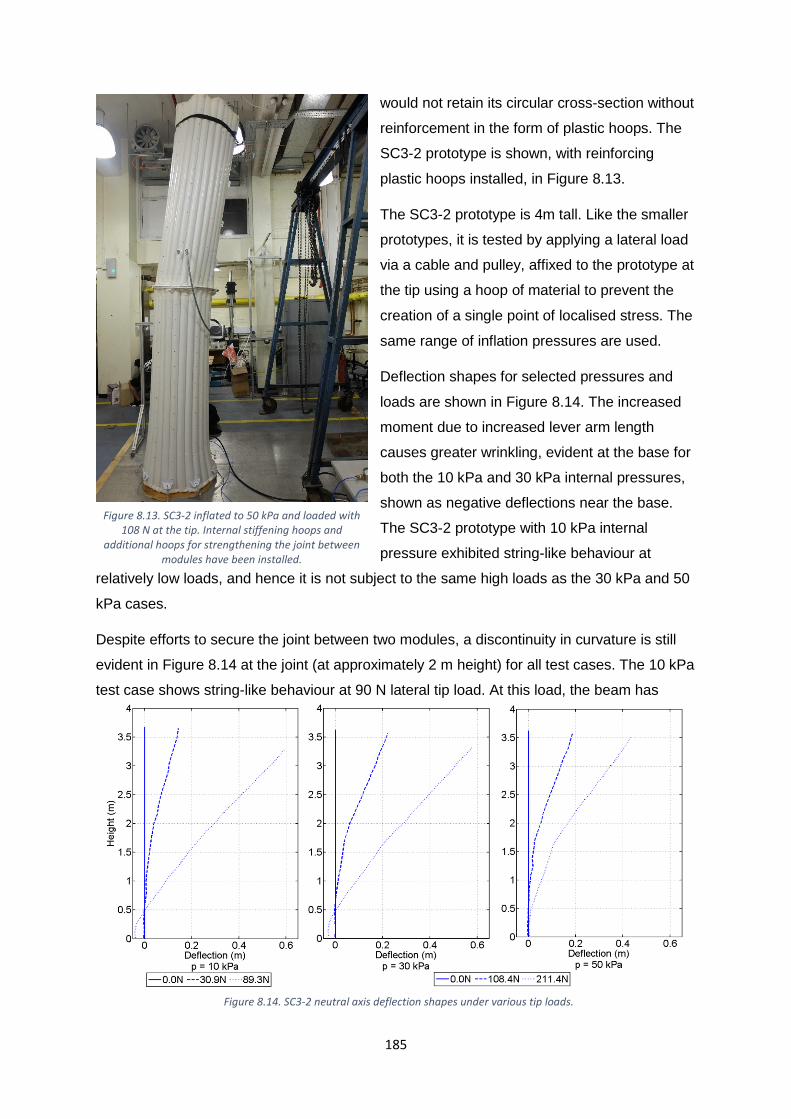
185
would not retain its circular cross-section without
reinforcement in the form of plastic hoops. The
SC3-2 prototype is shown, with reinforcing
plastic hoops installed, in Figure 8.13.
The SC3-2 prototype is 4m tall. Like the smaller
prototypes, it is tested by applying a lateral load
via a cable and pulley, affixed to the prototype at
the tip using a hoop of material to prevent the
creation of a single point of localised stress. The
same range of inflation pressures are used.
Deflection shapes for selected pressures and
loads are shown in Figure 8.14. The increased
moment due to increased lever arm length
causes greater wrinkling, evident at the base for
both the 10 kPa and 30 kPa internal pressures,
shown as negative deflections near the base.
The SC3-2 prototype with 10 kPa internal
pressure exhibited string-like behaviour at
relatively low loads, and hence it is not subject to the same high loads as the 30 kPa and 50
kPa cases.
Despite efforts to secure the joint between two modules, a discontinuity in curvature is still
evident in Figure 8.14 at the joint (at approximately 2 m height) for all test cases. The 10 kPa
test case shows string-like behaviour at 90 N lateral tip load. At this load, the beam has
Figure 8.13. SC3-2 inflated to 50 kPa and loaded with 108 N at the tip. Internal stiffening hoops and
additional hoops for strengthening the joint between modules have been installed.
Figure 8.14. SC3-2 neutral axis deflection shapes under various tip loads.
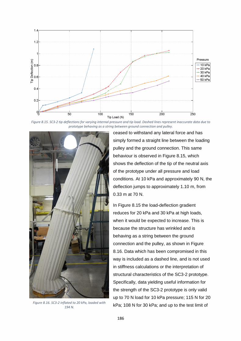
186
ceased to withstand any lateral force and has
simply formed a straight line between the loading
pulley and the ground connection. This same
behaviour is observed in Figure 8.15, which
shows the deflection of the tip of the neutral axis
of the prototype under all pressure and load
conditions. At 10 kPa and approximately 90 N, the
deflection jumps to approximately 1.10 m, from
0.33 m at 70 N.
In Figure 8.15 the load-deflection gradient
reduces for 20 kPa and 30 kPa at high loads,
when it would be expected to increase. This is
because the structure has wrinkled and is
behaving as a string between the ground
connection and the pulley, as shown in Figure
8.16. Data which has been compromised in this
way is included as a dashed line, and is not used
in stiffness calculations or the interpretation of
structural characteristics of the SC3-2 prototype.
Specifically, data yielding useful information for
the strength of the SC3-2 prototype is only valid
up to 70 N load for 10 kPa pressure; 115 N for 20
kPa; 108 N for 30 kPa; and up to the test limit of Figure 8.16. SC3-2 inflated to 20 kPa, loaded with
194 N.
Figure 8.15. SC3-2 tip deflections for varying internal pressure and tip load. Dashed lines represent inaccurate data due to prototype behaving as a string between ground connection and pulley.
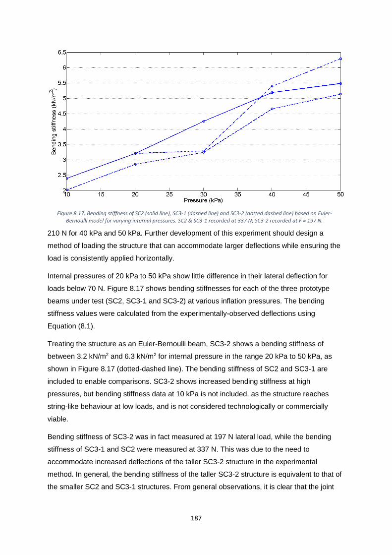
187
210 N for 40 kPa and 50 kPa. Further development of this experiment should design a
method of loading the structure that can accommodate larger deflections while ensuring the
load is consistently applied horizontally.
Internal pressures of 20 kPa to 50 kPa show little difference in their lateral deflection for
loads below 70 N. Figure 8.17 shows bending stiffnesses for each of the three prototype
beams under test (SC2, SC3-1 and SC3-2) at various inflation pressures. The bending
stiffness values were calculated from the experimentally-observed deflections using
Equation (8.1).
Treating the structure as an Euler-Bernoulli beam, SC3-2 shows a bending stiffness of
between 3.2 kN/m2 and 6.3 kN/m2 for internal pressure in the range 20 kPa to 50 kPa, as
shown in Figure 8.17 (dotted-dashed line). The bending stiffness of SC2 and SC3-1 are
included to enable comparisons. SC3-2 shows increased bending stiffness at high
pressures, but bending stiffness data at 10 kPa is not included, as the structure reaches
string-like behaviour at low loads, and is not considered technologically or commercially
viable.
Bending stiffness of SC3-2 was in fact measured at 197 N lateral load, while the bending
stiffness of SC3-1 and SC2 were measured at 337 N. This was due to the need to
accommodate increased deflections of the taller SC3-2 structure in the experimental
method. In general, the bending stiffness of the taller SC3-2 structure is equivalent to that of
the smaller SC2 and SC3-1 structures. From general observations, it is clear that the joint
Figure 8.17. Bending stiffness of SC2 (solid line), SC3-1 (dashed line) and SC3-2 (dotted dashed line) based on Euler-Bernoulli model for varying internal pressures. SC2 & SC3-1 recorded at 337 N; SC3-2 recorded at F = 197 N.
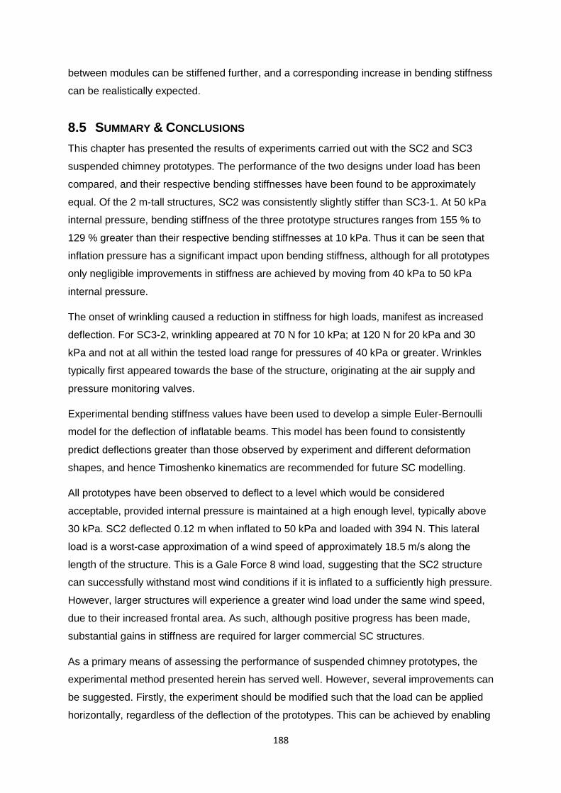
188
between modules can be stiffened further, and a corresponding increase in bending stiffness
can be realistically expected.
8.5 SUMMARY & CONCLUSIONS
This chapter has presented the results of experiments carried out with the SC2 and SC3
suspended chimney prototypes. The performance of the two designs under load has been
compared, and their respective bending stiffnesses have been found to be approximately
equal. Of the 2 m-tall structures, SC2 was consistently slightly stiffer than SC3-1. At 50 kPa
internal pressure, bending stiffness of the three prototype structures ranges from 155 % to
129 % greater than their respective bending stiffnesses at 10 kPa. Thus it can be seen that
inflation pressure has a significant impact upon bending stiffness, although for all prototypes
only negligible improvements in stiffness are achieved by moving from 40 kPa to 50 kPa
internal pressure.
The onset of wrinkling caused a reduction in stiffness for high loads, manifest as increased
deflection. For SC3-2, wrinkling appeared at 70 N for 10 kPa; at 120 N for 20 kPa and 30
kPa and not at all within the tested load range for pressures of 40 kPa or greater. Wrinkles
typically first appeared towards the base of the structure, originating at the air supply and
pressure monitoring valves.
Experimental bending stiffness values have been used to develop a simple Euler-Bernoulli
model for the deflection of inflatable beams. This model has been found to consistently
predict deflections greater than those observed by experiment and different deformation
shapes, and hence Timoshenko kinematics are recommended for future SC modelling.
All prototypes have been observed to deflect to a level which would be considered
acceptable, provided internal pressure is maintained at a high enough level, typically above
30 kPa. SC2 deflected 0.12 m when inflated to 50 kPa and loaded with 394 N. This lateral
load is a worst-case approximation of a wind speed of approximately 18.5 m/s along the
length of the structure. This is a Gale Force 8 wind load, suggesting that the SC2 structure
can successfully withstand most wind conditions if it is inflated to a sufficiently high pressure.
However, larger structures will experience a greater wind load under the same wind speed,
due to their increased frontal area. As such, although positive progress has been made,
substantial gains in stiffness are required for larger commercial SC structures.
As a primary means of assessing the performance of suspended chimney prototypes, the
experimental method presented herein has served well. However, several improvements can
be suggested. Firstly, the experiment should be modified such that the load can be applied
horizontally, regardless of the deflection of the prototypes. This can be achieved by enabling

189
the pulley to be raised or lowered as required. Bespoke solid-material end-caps for the
beams would ensure a built-in connection at the ground, preventing rotation of the base of
the prototype and removing the need to apply significant tension on the structure to secure it.
Such an approach would also ensure that the annular cross-section is maintained at the
base.
Beyond improving the experimental method, other issues worthy of further work have been
identified. These include developing a model to describe the deflection shape of the SC
prototype under load. A review of the relevant literature has led to the conclusion that
Bernoulli beam kinematics are insufficient for modelling larger structures and a Timoshenko
model is required. A mathematical treatment of the joint between modules will be required,
most likely modelling it as a stiff rotational spring. Load cases beyond single-point tip load
will also need to be explored, for example uniformly distributed loads, which are a good
approximation for simulating wind loading, especially on shorter structures.
A further prototype, SC4, has already been constructed to address and test the issues raised
in this analysis. SC4 is of the same scale as SC3-2 and, providing its performance is
satisfactory, it will inform the design and manufacture of SC5, a 20 m-tall SC prototype for
outdoor use. SC5 will enable careful analysis of the proposed commercial-scale SC design
and its operation under real-world conditions. It will be fully-instrumented to record strain on
the fabric surface and local weather conditions, to enable the correlation of load and strain
data. Successful operation of such a large-scale structure would significantly advance the
SC’s journey towards commercial deployment, a journey which has begun with the analyses
presented in this chapter.
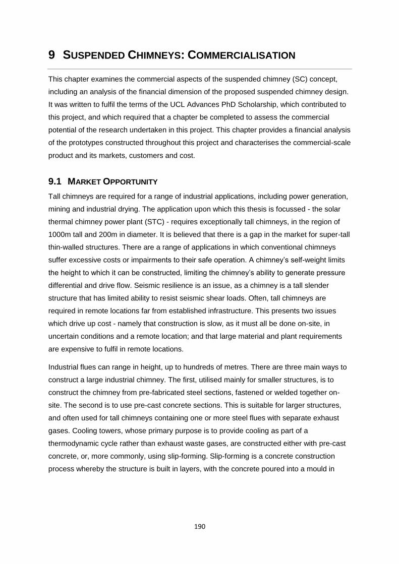
190
9 SUSPENDED CHIMNEYS: COMMERCIALISATION
This chapter examines the commercial aspects of the suspended chimney (SC) concept,
including an analysis of the financial dimension of the proposed suspended chimney design.
It was written to fulfil the terms of the UCL Advances PhD Scholarship, which contributed to
this project, and which required that a chapter be completed to assess the commercial
potential of the research undertaken in this project. This chapter provides a financial analysis
of the prototypes constructed throughout this project and characterises the commercial-scale
product and its markets, customers and cost.
9.1 MARKET OPPORTUNITY
Tall chimneys are required for a range of industrial applications, including power generation,
mining and industrial drying. The application upon which this thesis is focussed - the solar
thermal chimney power plant (STC) - requires exceptionally tall chimneys, in the region of
1000m tall and 200m in diameter. It is believed that there is a gap in the market for super-tall
thin-walled structures. There are a range of applications in which conventional chimneys
suffer excessive costs or impairments to their safe operation. A chimney’s self-weight limits
the height to which it can be constructed, limiting the chimney’s ability to generate pressure
differential and drive flow. Seismic resilience is an issue, as a chimney is a tall slender
structure that has limited ability to resist seismic shear loads. Often, tall chimneys are
required in remote locations far from established infrastructure. This presents two issues
which drive up cost - namely that construction is slow, as it must all be done on-site, in
uncertain conditions and a remote location; and that large material and plant requirements
are expensive to fulfil in remote locations.
Industrial flues can range in height, up to hundreds of metres. There are three main ways to
construct a large industrial chimney. The first, utilised mainly for smaller structures, is to
construct the chimney from pre-fabricated steel sections, fastened or welded together on-
site. The second is to use pre-cast concrete sections. This is suitable for larger structures,
and often used for tall chimneys containing one or more steel flues with separate exhaust
gases. Cooling towers, whose primary purpose is to provide cooling as part of a
thermodynamic cycle rather than exhaust waste gases, are constructed either with pre-cast
concrete, or, more commonly, using slip-forming. Slip-forming is a concrete construction
process whereby the structure is built in layers, with the concrete poured into a mould in
191
which steel reinforcement is laid if required. After each layer has set, the mould is removed
and the next layer is constructed. The scaffolding is designed in such a way that it remains
at the top of the structure and rises with it (see Figure 9.1).
This project is concerned with the suspended chimney concept, which aims to address
issues encountered when constructing tall chimneys from conventional materials. The
quantity of material consumed in building tall chimney structures, accompanied by the very
significant weight and wind forces that the structure will undergo suggests that some radical
re-thinking of the chimney structure itself is merited. The idea of a suspended chimney was
conceived – a chimney manufactured from industrial-strength films or fabrics and held aloft
with envelopes of lighter-than-air gas.
It became clear that this concept could mitigate further issues experienced by conventional
chimneys. These include height limitations due to self-weight, vulnerability to damage during
a seismic event, speed of construction on-site, and ease of construction in areas remote
from established infrastructure. Further details are provided in Table 9.1. Potential
customers will likely be those with a need for tall chimney structures, but in which the
operating environment lends greater appeal to the suspended chimney structure over a
conventional structure. Appendix IX characterises potential customers and suitable
geographic regions in more detail.
Figure 9.1. Slip-forming construction of natural-draft cooling tower [154]
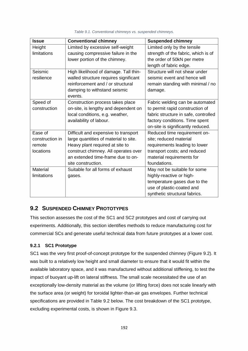
192
Table 9.1. Conventional chimneys vs. suspended chimneys.
Issue Conventional chimney Suspended chimney
Height
limitations
Limited by excessive self-weight
causing compressive failure in the
lower portion of the chimney.
Limited only by the tensile
strength of the fabric, which is of
the order of 50kN per metre
length of fabric edge.
Seismic
resilience
High likelihood of damage. Tall thin-
walled structure requires significant
reinforcement and / or structural
damping to withstand seismic
events.
Structure will not shear under
seismic event and hence will
remain standing with minimal / no
damage.
Speed of
construction
Construction process takes place
on-site, is lengthy and dependent on
local conditions, e.g. weather,
availability of labour.
Fabric welding can be automated
to permit rapid construction of
fabric structure in safe, controlled
factory conditions. Time spent
on-site is significantly reduced.
Ease of
construction in
remote
locations
Difficult and expensive to transport
large quantities of material to site.
Heavy plant required at site to
construct chimney. All operates over
an extended time-frame due to on-
site construction.
Reduced time requirement on-
site; reduced material
requirements leading to lower
transport costs; and reduced
material requirements for
foundations.
Material
limitations
Suitable for all forms of exhaust
gases.
May not be suitable for some
highly-reactive or high-
temperature gases due to the
use of plastic-coated and
synthetic structural fabrics.
9.2 SUSPENDED CHIMNEY PROTOTYPES
This section assesses the cost of the SC1 and SC2 prototypes and cost of carrying out
experiments. Additionally, this section identifies methods to reduce manufacturing cost for
commercial SCs and generate useful technical data from future prototypes at a lower cost.
9.2.1 SC1 Prototype
SC1 was the very first proof-of-concept prototype for the suspended chimney (Figure 9.2). It
was built to a relatively low height and small diameter to ensure that it would fit within the
available laboratory space, and it was manufactured without additional stiffening, to test the
impact of buoyant up-lift on lateral stiffness. The small scale necessitated the use of an
exceptionally low-density material as the volume (or lifting force) does not scale linearly with
the surface area (or weight) for toroidal lighter-than-air gas envelopes. Further technical
specifications are provided in Table 9.2 below. The cost breakdown of the SC1 prototype,
excluding experimental costs, is shown in Figure 9.3.
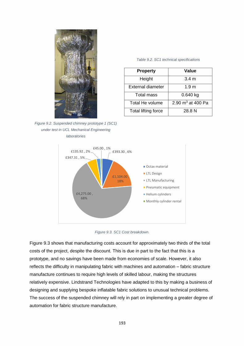
193
Figure 9.2. Suspended chimney prototype 1 (SC1)
under test in UCL Mechanical Engineering
laboratories
Table 9.2. SC1 technical specifications
Property Value
Height 3.4 m
External diameter 1.9 m
Total mass 0.640 kg
Total He volume 2.90 m3 at 400 Pa
Total lifting force 28.8 N
Figure 9.3. SC1 Cost breakdown.
Figure 9.3 shows that manufacturing costs account for approximately two thirds of the total
costs of the project, despite the discount. This is due in part to the fact that this is a
prototype, and no savings have been made from economies of scale. However, it also
reflects the difficulty in manipulating fabric with machines and automation – fabric structure
manufacture continues to require high levels of skilled labour, making the structures
relatively expensive. Lindstrand Technologies have adapted to this by making a business of
designing and supplying bespoke inflatable fabric solutions to unusual technical problems.
The success of the suspended chimney will rely in part on implementing a greater degree of
automation for fabric structure manufacture.
£393.30 , 6%
£1,104.00 , 18%
£4,275.00 , 68%
£347.31 , 5%
£135.92 , 2%£45.00 , 1%
Octax material
LTL Design
LTL Manufacturing
Pneumatic equipment
Helium cylinders
Monthly cylinder rental
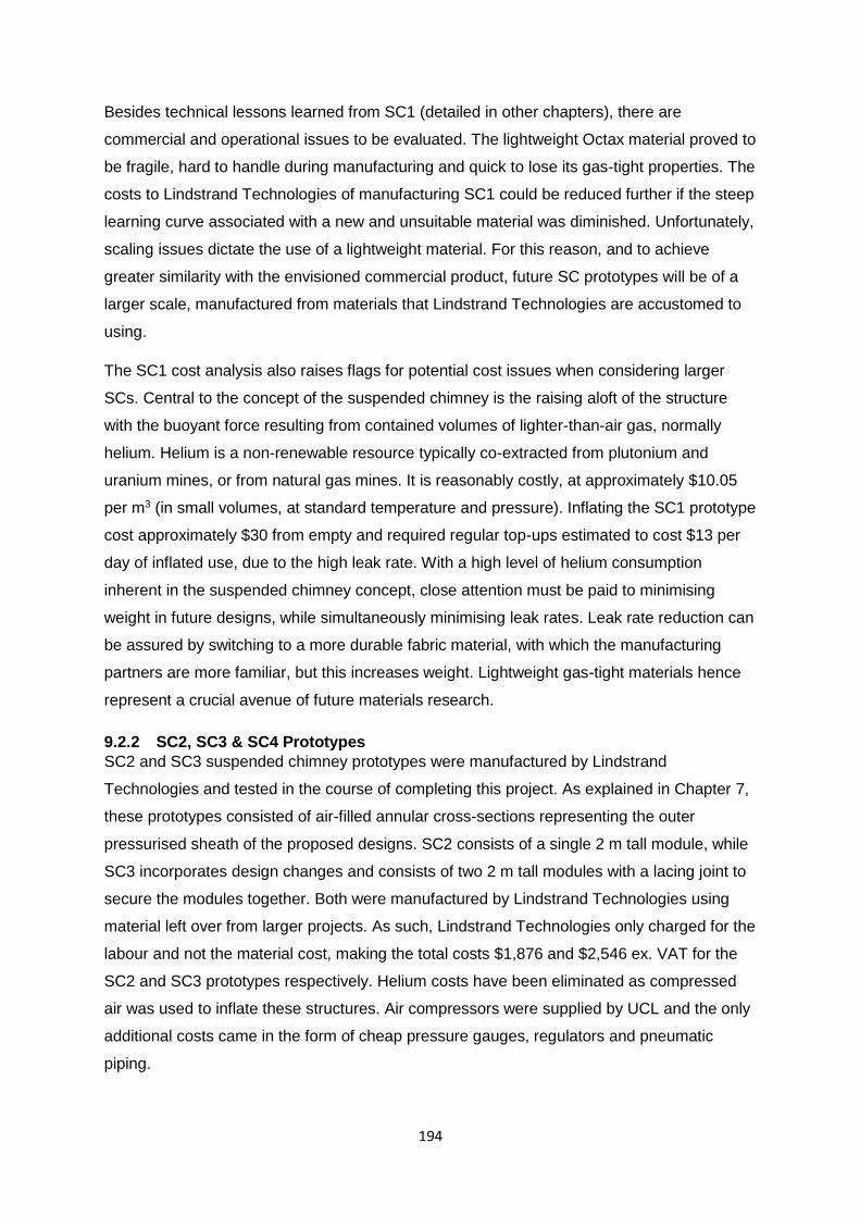
194
Besides technical lessons learned from SC1 (detailed in other chapters), there are
commercial and operational issues to be evaluated. The lightweight Octax material proved to
be fragile, hard to handle during manufacturing and quick to lose its gas-tight properties. The
costs to Lindstrand Technologies of manufacturing SC1 could be reduced further if the steep
learning curve associated with a new and unsuitable material was diminished. Unfortunately,
scaling issues dictate the use of a lightweight material. For this reason, and to achieve
greater similarity with the envisioned commercial product, future SC prototypes will be of a
larger scale, manufactured from materials that Lindstrand Technologies are accustomed to
using.
The SC1 cost analysis also raises flags for potential cost issues when considering larger
SCs. Central to the concept of the suspended chimney is the raising aloft of the structure
with the buoyant force resulting from contained volumes of lighter-than-air gas, normally
helium. Helium is a non-renewable resource typically co-extracted from plutonium and
uranium mines, or from natural gas mines. It is reasonably costly, at approximately $10.05
per m3 (in small volumes, at standard temperature and pressure). Inflating the SC1 prototype
cost approximately $30 from empty and required regular top-ups estimated to cost $13 per
day of inflated use, due to the high leak rate. With a high level of helium consumption
inherent in the suspended chimney concept, close attention must be paid to minimising
weight in future designs, while simultaneously minimising leak rates. Leak rate reduction can
be assured by switching to a more durable fabric material, with which the manufacturing
partners are more familiar, but this increases weight. Lightweight gas-tight materials hence
represent a crucial avenue of future materials research.
9.2.2 SC2, SC3 & SC4 Prototypes
SC2 and SC3 suspended chimney prototypes were manufactured by Lindstrand
Technologies and tested in the course of completing this project. As explained in Chapter 7,
these prototypes consisted of air-filled annular cross-sections representing the outer
pressurised sheath of the proposed designs. SC2 consists of a single 2 m tall module, while
SC3 incorporates design changes and consists of two 2 m tall modules with a lacing joint to
secure the modules together. Both were manufactured by Lindstrand Technologies using
material left over from larger projects. As such, Lindstrand Technologies only charged for the
labour and not the material cost, making the total costs $1,876 and $2,546 ex. VAT for the
SC2 and SC3 prototypes respectively. Helium costs have been eliminated as compressed
air was used to inflate these structures. Air compressors were supplied by UCL and the only
additional costs came in the form of cheap pressure gauges, regulators and pneumatic
piping.

195
Following the design assessment and technical analysis of the SC2 and SC3 prototypes, a
further two-module prototype has been ordered from Lindstrand Technologies, incorporating
design changes to resolve issues identified with SC3. According to a quote supplied by
Lindstrand Technologies, the SC4 prototype is expected to cost $2,546 ex. VAT.
9.2.3 SC5 Prototype
As the next scale up to 20 m height, the proposed SC5 prototype has been fully specified
and costed, with details provided in this section below. The SC5 design uses high-pressure
air-filled sheaths at the inner and outer surfaces of the helium envelopes to both maintain the
shape of the chimney section and provide lateral stiffening. Figure 9.5 gives a design
drawing to illustrate the concept while Table 9.3 gives the key technical specifications.
Inclusive of VAT, the total cost to manufacture and operate SC5 as a research prototype
over the course of a year is $67k. As with SC1, significant savings are made due to the
research partnership with Lindstrand Technologies Ltd, which is offering a discount on
manufacturing and a suitable location for installation and testing of the structure free of
charge. A breakdown of costs is supplied in Figure 9.4. SC5, like SC1, has the largest
proportion of its cost absorbed by manufacturing, at 75 %. Helium costs remain significant,
forecast at 9 % of the total to first inflation. Subsequent inflations and top-ups due to leaks
will increase this cost further. As such, it is imperative that future research should focus both
on minimising manufacturing costs and ensuring minimal leak rates, as this will have the
greatest impact upon total cost.
Figure 9.4. Project cost breakdown of SC5
$7,617
$40,200
$558
$5,008
$558 $2,233 Fabric material
Manufacturing
PneumaticequipmentHelium
Helium supplyequipmentInstrumentation
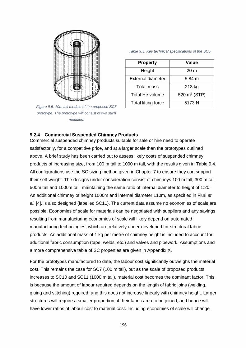
196
Figure 9.5. 10m tall module of the proposed SC5
prototype. The prototype will consist of two such
modules.
Table 9.3. Key technical specifications of the SC5
Property Value
Height 20 m
External diameter 5.84 m
Total mass 213 kg
Total He volume 520 m3 (STP)
Total lifting force 5173 N
9.2.4 Commercial Suspended Chimney Products
Commercial suspended chimney products suitable for sale or hire need to operate
satisfactorily, for a competitive price, and at a larger scale than the prototypes outlined
above. A brief study has been carried out to assess likely costs of suspended chimney
products of increasing size, from 100 m tall to 1000 m tall, with the results given in Table 9.4.
All configurations use the SC sizing method given in Chapter 7 to ensure they can support
their self-weight. The designs under consideration consist of chimneys 100 m tall, 300 m tall,
500m tall and 1000m tall, maintaining the same ratio of internal diameter to height of 1:20.
An additional chimney of height 1000m and internal diameter 110m, as specified in Fluri et
al. [4], is also designed (labelled SC11). The current data assume no economies of scale are
possible. Economies of scale for materials can be negotiated with suppliers and any savings
resulting from manufacturing economies of scale will likely depend on automated
manufacturing technologies, which are relatively under-developed for structural fabric
products. An additional mass of 1 kg per metre of chimney height is included to account for
additional fabric consumption (tape, welds, etc.) and valves and pipework. Assumptions and
a more comprehensive table of SC properties are given in Appendix X.
For the prototypes manufactured to date, the labour cost significantly outweighs the material
cost. This remains the case for SC7 (100 m tall), but as the scale of proposed products
increases to SC10 and SC11 (1000 m tall), material cost becomes the dominant factor. This
is because the amount of labour required depends on the length of fabric joins (welding,
gluing and stitching) required, and this does not increase linearly with chimney height. Larger
structures will require a smaller proportion of their fabric area to be joined, and hence will
have lower ratios of labour cost to material cost. Including economies of scale will change
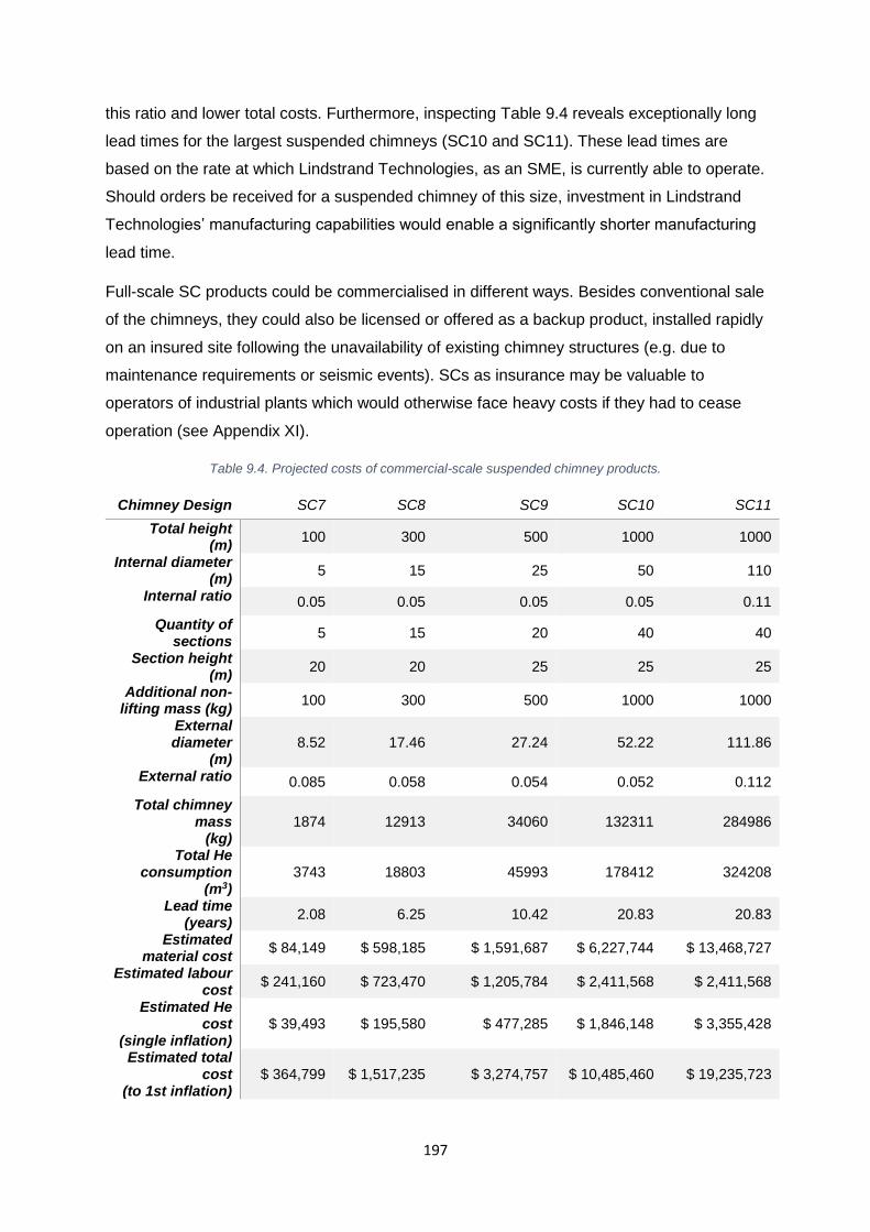
197
this ratio and lower total costs. Furthermore, inspecting Table 9.4 reveals exceptionally long
lead times for the largest suspended chimneys (SC10 and SC11). These lead times are
based on the rate at which Lindstrand Technologies, as an SME, is currently able to operate.
Should orders be received for a suspended chimney of this size, investment in Lindstrand
Technologies’ manufacturing capabilities would enable a significantly shorter manufacturing
lead time.
Full-scale SC products could be commercialised in different ways. Besides conventional sale
of the chimneys, they could also be licensed or offered as a backup product, installed rapidly
on an insured site following the unavailability of existing chimney structures (e.g. due to
maintenance requirements or seismic events). SCs as insurance may be valuable to
operators of industrial plants which would otherwise face heavy costs if they had to cease
operation (see Appendix XI).
Table 9.4. Projected costs of commercial-scale suspended chimney products.
Chimney Design SC7 SC8 SC9 SC10 SC11
Total height (m)
100 300 500 1000 1000
Internal diameter (m)
5 15 25 50 110
Internal ratio 0.05 0.05 0.05 0.05 0.11
Quantity of sections
5 15 20 40 40
Section height (m)
20 20 25 25 25
Additional non-lifting mass (kg)
100 300 500 1000 1000
External diameter
(m) 8.52 17.46 27.24 52.22 111.86
External ratio 0.085 0.058 0.054 0.052 0.112
Total chimney mass (kg)
1874 12913 34060 132311 284986
Total He consumption
(m3) 3743 18803 45993 178412 324208
Lead time (years)
2.08 6.25 10.42 20.83 20.83
Estimated material cost
$ 84,149 $ 598,185 $ 1,591,687 $ 6,227,744 $ 13,468,727
Estimated labour cost
$ 241,160 $ 723,470 $ 1,205,784 $ 2,411,568 $ 2,411,568
Estimated He cost
(single inflation) $ 39,493 $ 195,580 $ 477,285 $ 1,846,148 $ 3,355,428
Estimated total cost
(to 1st inflation) $ 364,799 $ 1,517,235 $ 3,274,757 $ 10,485,460 $ 19,235,723

198
9.3 SUSPENDED CHIMNEYS AND THE SOLAR THERMAL CHIMNEY POWER
PLANT This section compares the cost of a solar thermal chimney power plant with concrete and
suspended chimneys. These models assume that the STCs with suspended chimneys and
conventional chimneys both generate power at the same rate. Assumptions are made for
cost of raw materials and labour based on the figures supplied by Fluri et al. [4]. The key
dimensions of the solar thermal chimney power plant are supplied in Table 9.5. Solar
thermal chimney power plants have a key advantage over other forms of power plant - they
are relatively simple structures with minimal maintenance requirements. As such, plant
lifetimes (for concrete chimney structures) of 100 years have been posited [1]. This
investigation analyses the financial performance of the STC over a 100-year operational
lifetime, although the suspended chimney material will need replacing more regularly due to
abrasion by air-borne particles and UV degradation of the industrial fabrics. A design life of
20 years has been assumed for the suspended chimney. This has the advantage of
staggering the required capital investment and hence reducing borrowing requirements
compared to the conventional concrete chimney, where all costs must be met at the outset
of the project.
The costs calculated in this model are based on simple analyses of cost per unit area for the
collector and cost per unit volume for the concrete chimney. Labour and plant costs are
further extrapolated from the area of collector and volume of concrete consumed
respectively. Turbine and powerblock costs are based on an assumed cost per kilowatt of
peak power output. All the specific costs (per square metre; per cubic metre; and per
kilowatt) are obtained from a comprehensive cost analysis of STCs conducted by Fluri et
al.[4].
Suspended chimneys, as a novel product, have no body of literature upon which costs can
be based. Appendix X supplies a cost model of commercial-scale suspended chimneys,
based on manufacturing and cost data from Lindstrand Technologies Ltd. The largest SC in
the cost model (SC11) is of the same dimensions given in Table 9.5, and has a cost of $19.5
million. All assumptions are given in Appendix X. Table 9.6 shows the key performance of
STCs with both types of chimney. Financing costs are determined by factors such as cost of
debt, inflation, renewable energy incentives and tax credits. These factors vary hugely with
location, regulatory environments and economic conditions, and hence financial costs are
disregarded for this analysis.

199
Table 9.5. Solar thermal chimney power plant key dimensions
Parameter Value
Collector diameter 2300 m
Collector inlet height 4 m
Collector outlet height 11.5 m
Chimney height 1000 m
Chimney internal diameter 110 m
Peak power output 70 MW
Table 9.6. Key performance metrics of STCs with concrete or suspended chimneys
Performance metric STC with concrete
chimney
STC with suspended
chimney
Collector cost $593.7 M $593.7 M
Chimney cost $172.8 M $101.6 M
Turbine & powerblock
cost
$32.3 M $32.3 M
Total cost $878.6 M $825.4 M
Specific capital cost $ 13,000 /kW $ 11,800 /kW
Levelised electricity cost $ 0.053 /kWh $ 0.049 /kWh
(a) STC with suspended chimney
(b) STC with concrete chimney
Figure 9.6. Cost breakdown of STC structure with concrete or suspended chimneys.
Collector, $593,650,000 ,
65%
Chimney, $172,790,000 ,
19%
Turbines, $32,250,000 ,
4%
Contingency, $79,869,000 ,
9%
O&M, $27,839,987
, 3%
Collector$593,650,000
72%
Chimney$101,571,230
12%
Turbines$32,250,000
4%
Contingency$72,747,123
9%
O&M$27,839,987
3%

200
Figure 9.6 shows the cost breakdown for both STC types. Material and construction costs
are given in Table 9.6, while operation and maintenance (O&M) costs are defined for both
concrete and suspended chimney variants as being $1 million in the first year, growing at 2%
annually for the lifetime of the plant. The contingency funds are set at 10 % of the material
and construction expenditure (excluding operation and maintenance).
The STC with suspended chimney represents a net cost saving over concrete chimney
technology of 6.1 %, with the additional benefit, already identified, of staggering the cost of
the chimney across the lifetime of the plant. A series of five suspended chimneys, with a
lifetime equivalent to a single concrete chimney, incurs a cost of $101.6 million, 42 %
cheaper than its concrete alternative.
The collector accounts for the majority of the cost due to its scale. The chimney, while
representing a smaller proportion of the total cost (whether concrete or suspended
chimneys), represents a large proportion of the total engineering risk, and hence is expected
to impose significant financial costs (e.g. insurance), which are excluded from the current
model. These costs will exist for both concrete chimneys and suspended chimneys. The
suspended chimney is still relatively immature, and it is envisioned that further cost savings
can be achieved, especially in the fields of manufacturing automation and reducing leak
rates to conserve expensive helium. Further cost-saving developments will make the
suspended chimney even more competitive compared to the concrete chimney for the STC
power plant application.
9.4 CONCLUDING REMARKS This chapter has assessed the financial implications of developing the suspended chimney
product. The overall cost of solar thermal chimney power plants has been assessed, with
both concrete and suspended chimneys. The suspended chimney achieves a total cost
saving of 6.1 % for the whole STC plant, compared to the concrete chimney. As a
component, a series of five suspended chimneys costs 41 % less than an equivalent-sized
concrete chimney with the same expected lifetime. This suggests that the suspended
chimney is a technology worth pursuing further in its potential for cost saving for tall chimney
structures.
Besides the cost savings already predicted, it is envisioned that various improvements can
be made to SC design and manufacturing processes, especially in improving economies of
scale and reducing lead times for manufacturing suspended chimneys. Future work should
therefore focus on reducing costs by minimising leak rates, maximising manufacturing
automation and ensuring reliable supplies of helium and structural fabrics. If these

201
improvements are rigorously pursued, even more cost-effective suspended chimneys could
be developed, and would be expected to compete effectively with conventional concrete
chimney structures.

202
10 CONCLUSIONS
This thesis has pursued two separate but interconnected research topics. The first examined
thermodynamic principles of operation behind the solar thermal chimney (STC) power plant
and analysed proposed design changes to increase power output and improve ease of
construction. The second research topic consisted of an analysis of the suspended chimney
innovation, a lighter-than-air or air-filled fabric chimney structure to replace the tall thin-shell
chimney structure required by the STC power plant. Throughout the whole thesis, the
interconnecting theme is the STC power plant and efforts to bring STC technology closer to
commercialisation, via incremental improvement (STC dimension matching and canopy
design analysis) and via radical innovation (the suspended chimney).
10.1 SOLAR THERMAL CHIMNEYS: LITERATURE REVIEW
Chapter 2 presented a comprehensive literature review of the modelling, experiments and
analysis relating to the STC power plant. Emerging from this review was the conclusion that
the thermodynamic operation of STC power plants was reasonably well-understood, but that
efforts to move the technology towards commercial viability were limited. The review
identified that while multiple optimisation studies of STC dimensions exist, the underlying
thermodynamic models are typically simplified, mostly lacking detailed determination of the
heat transfer coefficients within the collector. As such, there was a gap in the literature
whereby a comprehensive model could be used to identify best-performing matched
dimensions, in which the size of each component is matched to the other components of the
plant for optimum power output.
A further issue was identified in which the collector canopy profiles used in most models are
not in the form in which they would be manufactured, representing either unrealistic
complexity (and unnecessary cost) in the case of the exponential canopy, or requiring
exceptionally high levels of manufacturing accuracy in the case of the linearly sloped
canopy. In the process of designing for construction, these canopies would be simplified with
linear profiles and steps, and there remained a question over the impact this would have on
STC power output. Taken together, the contributions on these two topics aim to reduce cost
and construction complexity, and improve the economic viability of STC technology.
10.2 SOLAR THERMAL CHIMNEYS: MODELLING In order to assess the performance of different STC design configurations, a comprehensive
steady-state thermodynamic model was created, as described in Chapter 3. It incorporated a
full thermodynamic treatment of the collector, with three distinct collector components: the
203
ground surface; the working air; and the canopy, all connected through a system of linear
First Law equations. Any combination of geometric STC parameters and material properties
can be specified. The model is highly flexible, computationally efficient, and able to assess
the impact of different design choices upon performance. Experimental validation of the
modelling of such large structures is hard to achieve with a high degree of certainty, as no
commercial-scale STC power plants have been built. Instead, consensus is built through
comparing the outputs of different models by different authors. The model presented herein
generates power outputs within 5 % of models published in the literature.
10.3 SOLAR THERMAL CHIMNEYS: PARAMETRIC INVESTIGATIONS In Chapter 4, this thesis introduced the novel concept of dimension matching. It was
observed that, for certain configurations of chimney dimensions, STC power output would
cease to increase despite large increases in collector size, suggesting that the collector and
chimney were not suitably matched. It was found that for an over-sized collector, the
temperatures of the collector’s thermodynamic components were asymptotically approaching
equilibrium, meaning that increasing the collector size further did not result in a net increase
in heat transfer to the working air and thus did not result in increased power generation. The
best-performing configuration for a STC power plant, given a set of environmental conditions
and a chimney height, was found to be one in which the working air enters thermal
equilibrium at the chimney outlet (or close to it). This novel method enabled sets of best-
performing dimensions to be identified and the mechanism underlying this behaviour to be
determined.
A simple cost model was created based on non-dimensionalised cost units and it introduced
an additional criterion of power generated per unit cost, to enable the most cost-effective
configuration to be identified. For the given reference conditions used throughout this thesis,
the best-performing STC plant was identified as having a chimney 1000 m tall, with a flow
radius of 140 m; and a collector of radius 2800 m. This configuration generated almost 200
MW peak power output, similar to other models in the literature. Moreover, the discovery of
this mechanism is a useful tool for future STC researchers to determine whether their
chosen configuration is optimal.
10.4 SOLAR THERMAL CHIMNEYS: DESIGN FOR CONSTRUCTION The thermodynamic STC model was used to assess the impact upon STC performance of
different collector canopy profiles. Some of the canopy profiles used within the literature
reduce STC performance, or are impractical to construct. Chapter 5 assessed the
performance of the reference STC with different canopy profiles, identifying the best-

204
performing geometries for each canopy type and comparing between canopy types. The
detailed thermodynamic model of the collector enabled an in-depth analysis of air pressure,
velocity and temperature throughout the collector radial path, permitting additional insight to
be obtained.
It was found that the exponential canopy performed best, a result replicated elsewhere in the
literature. The exponential canopy profile for b = 0.42 remained low for the majority of the
radial path, keeping working air velocity high and promoting heat transfer. Flat canopies,
also commonly used, are simple to construct but underperform significantly. As a result, two
additional canopy profiles were analysed, based on construction-friendly approximations of
the best-performing canopy designs. The first, named the segmented canopy profile, kept a
low flat canopy for the majority of the radial path and then rose linearly to a specified outlet
height. The best-performing segmented canopy yielded nearly the same power output as the
exponential canopy, but with a simplified canopy design which will be easier to construct and
maintain. Chapter 5 also analysed a segmented stepped profile with three equal-height
steps, which yielded a power output only 5 % lower than the optimum. This canopy profile
requires only 1.5 % of the canopy area to be raised (and to reasonable heights), as opposed
to 9 % for the optimal segmented profile.
The best-performing configurations delivered the highest air temperatures at the collector
outlet. The segmented canopy profile delivers both a high chimney inlet air velocity and a
large pressure difference generated by the collector (prior to entering the chimney). These
two factors together determine the power output and hence the segmented and segmented-
stepped profiles are considered worthy of further analysis as potential canopy profiles for
commercial-scale STCs.
10.5 SUSPENDED CHIMNEYS: LITERATURE REVIEW
The research undertaken into solar thermal chimney power plant dimensions and collector
design represents a contribution to the gradual improvement of STC technology. The second
research topic contained within this thesis evaluates a radical innovation, namely the
suspended chimney, and assesses its potential for further development. To investigate the
viability of this concept, three laboratory-scale prototypes have been designed, constructed,
and tested in collaboration with Lindstrand Technologies Ltd, the industrial partner for this
EngD project. This thesis has reported on the design and manufacturing processes,
identifying and resolving issues. It also presented an experimental analysis of the
performance of the prototypes under lateral loading.

205
A review of existing literature, carried out in Chapter 6, revealed several important points.
Exceptionally tall thin-walled shell structures such as STC chimneys would develop
problems with stability due to self-weight and wind loading. Wind loads can be modelled with
some certainty up to approximately 300 m in height, but only tentative models exist beyond
this height. This project proposed inflatable suspended chimneys as a solution to the issues
of constructing large-scale chimney structures. Suspended chimneys are generally not
considered in the research literature, but a body of research does exist on the deflection
behaviour of inflatable beams. The literature comprises experimental analyses and
theoretical models, both analytical and finite element. Due to the nature of inflatable beams,
the body of literature is limited to modelling and testing the simple circular cross-section.
There exists a gap in the literature for the study of different cross-sections required by
structures such as the proposed suspended chimney, which requires an annular cross-
section. This thesis has provided experimental data regarding the deflection of such a
structure.
10.6 SUSPENDED CHIMNEYS: DESIGN DEVELOPMENT Chapter 7 assessed the designs and the ease of manufacture of the suspended chimney
prototypes manufactured during this investigation. The first-generation prototype, SC1, was
designed as a proof-of-concept prototype, testing the capability of enclosed helium volumes
to support a chimney structure. An exceptionally lightweight fabric was found in order to
alleviate scaling issues, whereby the lifting volume did not scale linearly with the surface
area, which comprised most of the mass. The prototype operated successfully, but – as it
was designed without lateral stiffening – it deflected significantly under load. The lightweight
material proved to be prone to high leak rates and valves and connections on the fabric
surface had sufficient mass to operate as point loads on the structure, causing it to deflect
before any external load was applied.
Following lessons learned from the SC1 prototype, a suspended chimney design was drawn
up, in which the helium volume which lifts the structure is bounded by thin high-pressure air-
inflated sheathes at the inner and outer walls. This design is significantly stiffer than earlier
designs without adding weight, as the air-filled sheathes contain the helium volume and
reduce the fabric area that would otherwise be used to maintain its shape.
SC3 was manufactured to test proposed improvements arising from the experience of using
SC2. A new way of manufacturing the structure was devised, and the issue of joining one
module to another needed testing, for which a joining method using tie lacing was
implemented. The SC3 structure had thinner walls than SC2, but did not form an annular
cross section once pressurised, and it required internal reinforcement in the form of plastic
206
hoops. The joint between modules proved to be too loose, also requiring reinforcement. As
such, the manufacturing methods used for SC2 were considered to be preferable.
SC4 – a further prototype also consisting of two 2 m tall modules – has recently been
commissioned and manufactured, incorporating the lessons learned from SC2 and SC3 in
the course of this project. The design and methods of manufacture are closer to SC2, with
improved connections to the ground and between modules. SC4 aims to resolve the issues
identified with joining modules in SC3-2. Once SC4 has been shown to operate satisfactorily,
any further design improvements will be included in SC5, a 20 m tall fully-instrumented SC
prototype for outdoor use, for which a design already exists. The successful operation of
SC5 will prove a major milestone on the journey towards a commercial-scale suspended
chimney, a journey begun with the feasibility study carried out for this project.
10.7 SUSPENDED CHIMNEYS: DATA ANALYSIS In Chapter 8, the prototypes were tested experimentally to assess their bending stiffness.
The SC2 prototype was built as a 1:10 scaled version of the outer air-filled sheath of a
planned 20 m suspended chimney structure. The SC2 prototype, and the subsequent SC3-1
and SC3-2 prototypes, were tested by applying a lateral load at the tip of the structure and
recording deflection states with high-resolution photographs. Deflection shapes were then
calculated for varying lateral tip load and internal pressure.
SC2 operated successfully and withstood relatively large tip loads without substantial
deflections. Increasing the internal pressure led to an increase in stiffness and a
corresponding decrease in deflection. Inflated to 50 kPa, the tip deflected by 0.12 m when
loaded with 394 N, equivalent to a wind loading of 18.5 m/s on a 2 m tall structure. Further
investigation is merited before firm conclusions can be drawn. Low pressures and high loads
caused wrinkles to appear on the fabric surface, as described in the literature. Wrinkled
fabric behaves differently, with reduced stiffness. SC3 was tested in both its 2 m
configuration (SC3-1) and its 4 m configuration (SC3-2). SC3-1 proved to have a stiffness
consistently about 10% lower than SC2 for all internal pressures, while SC3-2 was similar to
SC2. Large loads on the SC3-2 structure caused it to collapse and behave as a string,
limiting the maximum load for useful data analysis.
This research represents the first investigation of the suspended chimney innovation, and it
has concluded that the concept has potential, with the prototype structures resisting
considerable lateral load.
207
10.8 SUSPENDED CHIMNEYS: COMMERCIALISATION In Chapter 9, an analysis is provided of the costs of the prototypes manufactured for this
project, the proposed large-scale prototypes, and the proposed commercial-scale SC
products. The cost models are based on a cost per square metre of fabric consumed for
both materials and labour, with additional costs quantified based on industry data for helium
and helium supply equipment (where helium is used). Further costs include sensors and
instrumentation. SC2 and SC3 both cost under $2,600 to manufacture. A commercial-scale
SC structure, of the same size as the reference STC chimney (height 1000 m; internal
diameter 110 m) is projected to cost $19.3 million to build to first inflation, not including
financing costs, subsequent helium top-ups or any necessary groundworks. For the solar
thermal chimney power plant, this indicates that the reference plant would deliver electricity
at a levelized electricity cost (LEC) of $ 0.049 /kWh if using suspended chimneys versus a
LEC of $0.053 /kWh using a conventional concrete chimney, demonstrating that the
suspended chimney has the potential to deliver a 7.5 % cost saving over conventional
concrete chimneys in STC power plants.
10.9 CONCLUDING REMARKS
Solar thermal chimney technology continues to progress towards commercialisation. The
findings detailed in this thesis are intended as a contribution to the state of the art for solar
thermal chimney power plants, comprising a proposed method for identifying the best-
performing STC configurations and an appraisal of construction-friendly canopy profile
designs.
This thesis has also started the suspended chimney innovation down the road of
technological development. The design proposed herein, where the helium-filled lifting
volume is constrained by high-pressure air-filled sheathes that also provide structural
stiffness, remains to be assessed in its entirety, though the work presented on the air-
inflated sheathes suggests that they hold promise in terms of stiffening the suspended
chimney structure against wind loads. Continued research into these two related topics is
strongly recommended to ensure that the greatest possible benefits can be obtained from
the opportunities they present.
208
11 REFERENCES
[1] R. Harte, R. Höffer, W. B. Krätzig, P. Mark, and H. J. Niemann, “Solar updraft power
plants: Engineering structures for sustainable energy generation,” Eng. Struct., vol.
56, pp. 1698–1706, 2013.
[2] Schlaich Bergermann und Partner, “Solar updraft tower,” 2011.
[3] M. A. dos S. Bernardes, A. Voß, and G. Weinrebe, “Thermal and technical analyses
of solar chimneys,” Sol. Energy, vol. 75, no. 6, pp. 511–524, Dec. 2003.
[4] T. P. Fluri, J. P. Pretorius, C. Van Dyk, T. W. Von Backström, D. G. Kröger, and G. P.
a. G. Van Zijl, “Cost analysis of solar chimney power plants,” Sol. Energy, vol. 83, no.
2, pp. 246–256, Feb. 2009.
[5] A. J. Gannon and T. W. von Backström, “Solar Chimney Cycle Analysis With System
Loss and Solar Collector Performance,” J. Sol. Energy Eng., vol. 122, pp. 133–137,
2000.
[6] W. Haaf, K. Friedrich, G. Mayr, and J. Schlaich, “Solar Chimneys Part I: Principle and
Construction of the Pilot Plant in Manzanares,” Int. J. Sol. Energy, vol. 2, pp. 3–20,
1983.
[7] M. A. dos S. Bernardes, “Solar Chimney Power Plants – Developments and
Advancements,” in Solar Energy, 2010, pp. 171–186.
[8] T. Hamilton, Mad Like Tesla: Underdog Inventors and Their Relentless Pursuit of
Clean Energy. Ontario: ECW Press, 2011.
[9] W. Haaf, “Solar Chimneys Part II: Preliminary Test Results from the Manzanares Pilot
Plant,” Int. J. Sol. Energy, vol. 2, pp. 141–161, 1984.
[10] X. Zhou, J. Yang, B. Xiao, and G. Hou, “Simulation of a pilot solar chimney thermal
power generating equipment,” Renew. Energy, vol. 32, no. 10, pp. 1637–1644, 2007.
[11] M. O. Hamdan, “Analysis of a solar chimney power plant in the Arabian Gulf region,”
Renew. Energy, vol. 36, no. 10, pp. 2593–2598, Oct. 2011.
[12] J. Schlaich, R. Bergermann, W. Schiel, and G. Weinrebe, “Design of Commercial
Solar Updraft Tower Systems—Utilization of Solar Induced Convective Flows for
Power Generation,” J. Sol. Energy Eng., vol. 127, no. 1, p. 117, 2005.
[13] M. M. Padki and S. A. Sherif, “On a simple analytical model for solar chimneys,” Int. J.
Energy Res., vol. 349, pp. 345–349, 1999.
[14] N. Pasumarthi and S. A. Sherif, “Experimental and theoretical performance of a
demonstration solar chimney model - Part I: Mathematical model development,” Int. J.
Energy Res., vol. 22, no. 3, pp. 277–288, 1998.
[15] N. Pasumarthi and S. A. Sherif, “Experimental and theoretical performance of a
demonstration solar chimney model - Part II: experimental and theoretical results and

209
economic analysis,” Int. J. Energy Res., vol. 22, no. 5, pp. 443–461, 1998.
[16] J. P. Pretorius and D. G. Kröger, “Solar Chimney Power Plant Performance,” J. Sol.
Energy Eng., vol. 128, pp. 302–311, May 2006.
[17] X. Zhou and Y. Xu, “Solar updraft tower power generation,” Sol. Energy, 2014.
[18] M. A. dos S. Bernardes, R. M. Valle, and M. F. B. Cortez, “Numerical analysis of
natural laminar convection in a radial solar heater,” Int. J. Therm. Sci., vol. 38, pp. 42–
50, 1999.
[19] M. A. dos S. Bernardes, “Technische, ökonomische und ökologische Analyse von
Aufwind-kraftwerken,” Universität Stuttgart, 2004.
[20] M. A. dos S. Bernardes, T. von Backström, and D. Kröger, “Analysis of some
available heat transfer coefficients applicable to solar chimney power plant collectors,”
Sol. Energy, vol. 83, no. 2, pp. 264–275, 2009.
[21] J. P. Pretorius and D. G. Kröger, “Sensitivity Analysis of the Operating and Technical
Specifications of a Solar Chimney Power Plant,” J. Sol. Energy Eng., vol. 129, no. 2,
p. 171, 2007.
[22] D. G. Kröger and J. D. Buys, “Performance Evaluation of a Solar Chimney Power
Plant,” in ISES 2001 Solar World Congress, 2001.
[23] J. P. Pretorius, “Solar Tower Power Plant Performance Characteristics,” University of
Stellenbosch, 2004.
[24] F. Lupi, C. Borri, R. Harte, W. B. Krätzig, and H.-J. Niemann, “Facing technological
challenges of Solar Updraft Power Plants,” J. Sound Vib., vol. 334, pp. 57–84, 2015.
[25] W. B. Krätzig, “An integrated computer model of a solar updraft power plant,” Adv.
Eng. Softw., vol. 62–63, pp. 33–38, Aug. 2013.
[26] W. B. Krätzig, “Physics, computer simulation and optimization of thermo-
fluidmechanical processes of solar updraft power plants,” Sol. Energy, vol. 98, pp. 2–
11, 2013.
[27] W. B. Krätzig, “Solar Updraft Power Technology : Fighting Global Warming and Rising
Energy Costs,” J. Technol. Innov. Renew. Energy, vol. 4, pp. 52–64, 2015.
[28] R. A. Hedderwick, “Performance Evaluation of a Solar Chimney Power Plant,”
University of Stellenbosch, 2000.
[29] C. B. Maia, A. G. Ferreira, R. M. Valle, and M. F. B. Cortez, “Theoretical evaluation of
the influence of geometric parameters and materials on the behavior of the airflow in a
solar chimney,” Comput. Fluids, vol. 38, no. 3, pp. 625–636, 2009.
[30] R. Petela, “Thermodynamic study of a simplified model of the solar chimney power
plant,” Sol. Energy, vol. 83, no. 1, pp. 94–107, 2009.
[31] M. A. dos S. Bernardes, “Preliminary stability analysis of the convective symmetric
converging flow between two nearly parallel stationary disks similar to a solar updraft

210
power plant collector,” Sol. Energy, vol. 141, pp. 297–302, 2017.
[32] M. A. dos S. Bernardes, “Correlations for the symmetric converging flow and heat
transfer between two nearly parallel stationary disks similar to a solar updraft power
plant collector,” Sol. Energy, vol. 146, pp. 309–318, 2017.
[33] A. A. Gitan, S. H. Abdulmalek, and S. S. Dihrab, “Tracking collector consideration of
tilted collector solar updraft tower power plant under Malaysia climate conditions,”
Energy, vol. 93, pp. 1467–1477, 2015.
[34] M. Tingzhen, L. Wei, and X. Guoliang, “Analytical and numerical investigation of the
solar chimney power plant systems,” Int. J. Energy Res., vol. 30, no. 11, pp. 861–873,
2006.
[35] H. Pastohr, O. Kornadt, and K. Gürlebeck, “Numerical and analytical calculations of
the temperature and flow field in the upwind power plant,” Int. J. Energy Res., vol. 28,
no. 6, pp. 495–510, 2004.
[36] R. Sangi, M. Amidpour, and B. Hosseinizadeh, “Modeling and numerical simulation of
solar chimney power plants,” Sol. Energy, vol. 85, no. 5, pp. 829–838, 2011.
[37] X. Zhou, J. Yang, B. Xiao, G. Hou, and F. Xing, “Analysis of chimney height for solar
chimney power plant,” Appl. Therm. Eng., vol. 29, no. 1, pp. 178–185, 2009.
[38] N. Ninic, “Available energy of the air in solar chimneys and the possibility of its
ground-level concentration,” Sol. Energy, vol. 80, no. 7, pp. 804–811, 2006.
[39] T. P. Fluri and T. von Backström, “Comparison of modelling approaches and layouts
for solar chimney turbines,” Sol. Energy, vol. 82, no. 3, pp. 239–246, 2008.
[40] A. J. Gannon and T. W. von Backström, “Solar Chimney Turbine Performance,” J.
Sol. Energy Eng., vol. 125, no. 1, p. 101, 2003.
[41] T. W. von Backström and A. J. Gannon, “Solar chimney turbine characteristics,” Sol.
Energy, vol. 76, pp. 235–241, 2004.
[42] T. W. von Backström and T. P. Fluri, “Maximum fluid power condition in solar chimney
power plants – An analytical approach,” Sol. Energy, vol. 4, no. 11, pp. 1417–1423,
2006.
[43] S. Nizetic and B. Klarin, “A simplified analytical approach for evaluation of the optimal
ratio of pressure drop across the turbine in solar chimney power plants,” Appl. Energy,
vol. 87, no. 2, pp. 587–591, 2010.
[44] G. Xu, T. Ming, Y. Pan, F. Meng, and C. Zhou, “Numerical analysis on the
performance of solar chimney power plant system,” Energy Convers. Manag., vol. 52,
no. 2, pp. 876–883, 2011.
[45] X. Zhou, F. Wang, and R. M. Ochieng, “A review of solar chimney power technology,”
Renew. Sustain. Energy Rev., vol. 14, no. 8, pp. 2315–2338, 2010.
[46] J. P. Pretorius and D. G. Kröger, “Critical evaluation of solar chimney power plant
211
performance,” Sol. Energy, vol. 128, no. 5, pp. 535–544, May 2006.
[47] J. H. M. Beyers, “A Finite Volume Method for the Analysis of the Thermo-Flow Field of
a Solar Chimney Collector,” Stellenbosch University, 2000.
[48] J. H. M. Beyers, T. M. Harms, and D. G. Kröger, “A Finite Volume Analysis of
Turbulent Convective Heat Transfer for Accelerating Radial Flows,” Numer. Heat
Transf., vol. 40, no. 2, pp. 117–138, 2001.
[49] A. Koonsrisuk and T. Chitsomboon, “Partial geometric similarity for solar chimney
power plant modeling,” Sol. Energy, vol. 83, no. 9, pp. 1611–1618, 2009.
[50] A. Koonsrisuk and T. Chitsomboon, “Dynamic similarity in solar chimney modeling,”
Sol. Energy, vol. 81, no. 12, pp. 1439–1446, 2007.
[51] A. Koonsrisuk and T. Chitsomboon, “A single dimensionless variable for solar
chimney power plant modeling,” Sol. Energy, vol. 83, no. 12, pp. 2136–2143, 2009.
[52] K. M. Shirvan, S. Mirzakhanlari, M. Mamourian, and S. A. Kalogirou, “Optimization of
effective parameters on solar updraft tower to achieve potential maximum power
output: A sensitivity analysis and numerical simulation,” Appl. Energy, vol. 195, pp.
725–737, 2017.
[53] P. J. Cottam, P. Duffour, P. Lindstrand, and P. Fromme, “Effect of canopy profile on
solar thermal chimney performance,” Sol. Energy, vol. 129, pp. 286–296, 2016.
[54] M.-H. Huang, L. Chen, Y. L. He, J.-J. Cao, and W.-Q. Tao, “A two-dimensional
simulation method of the solar chimney power plant with a new radiation model for the
collector,” Int. Commun. Heat Mass Transf., vol. 85, pp. 100–106, 2017.
[55] T. Ming, X. Wang, R. K. de Richter, W. Liu, T. Wu, and Y. Pan, “Numerical analysis
on the influence of ambient crosswind on the performance of solar updraft power plant
system,” Renew. Sustain. Energy Rev., vol. 16, no. 8, pp. 5567–5583, 2012.
[56] X. Zhou, M. A. do. S. Bernardes, and R. M. Ochieng, “Influence of atmospheric cross
flow on solar updraft tower inflow,” Energy, vol. 42, no. 1, pp. 393–400, 2012.
[57] T. Ming, J. Gui, R. K. de Richter, Y. Pan, and G. Xu, “Numerical analysis on the solar
updraft power plant system with a blockage,” Sol. Energy, vol. 98, pp. 58–69, 2013.
[58] W. Shen, T. Ming, Y. Ding, Y. Wu, and R. K. de Richter, “Numerical analysis on an
industrial-scaled solar updraft power plant system with ambient crosswind,” Renew.
Energy, vol. 68, pp. 662–676, 2014.
[59] T. Ming, Y. Wu, R. K. de Richter, W. Liu, and S. A. Sherif, “Solar updraft power plant
system: A brief review and a case study on a new system with radial partition walls in
its collector,” Renew. Sustain. Energy Rev., vol. 69, pp. 472–487, 2017.
[60] T. W. von Backström and A. J. Gannon, “Compressible Flow Through Solar Power
Plant Chimneys,” J. Sol. Energy Eng., vol. 122, no. 3, p. 138, 2000.
[61] T. W. von Backström, “Calculation of pressure and density in solar power plant
212
chimneys,” J. Sol. Energy Eng., vol. 125, no. 1, p. 117, 2003.
[62] M. Lebbi, T. Chergui, H. Boualit, and I. Boutina, “Influence of geometric parameters
on the hydrodynamics control of solar chimney,” Int. J. Hydrogen Energy, vol. 39, no.
27, 2014.
[63] T. Chergui, S. Larbi, and A. Bouhdjar, “Thermo-hydrodynamic aspect analysis of flows
in solar chimney power plants—A case study,” Renew. Sustain. Energy Rev., vol. 14,
no. 5, pp. 1410–1418, 2010.
[64] M. Tingzhen, L. Wei, X. Guoling, X. Yanbin, G. Xuhu, and P. Yuan, “Numerical
simulation of the solar chimney power plant systems coupled with turbine,” Renew.
Energy, vol. 33, no. 5, pp. 897–905, 2008.
[65] A. Kasaeian, A. R. Mahmoudi, F. R. Astaraei, and A. Hejab, “3D simulation of solar
chimney power plant considering turbine blades,” Energy Convers. Manag., vol. 147,
pp. 55–65, 2017.
[66] A. B. Kasaeian, E. Heidari, and N. Vatan, “Experimental investigation of climatic
effects on the efficiency of a solar chimney pilot power plant,” Renew. Sustain. Energy
Rev., vol. 15, no. 9, pp. 5202–5206, 2011.
[67] Y. Wei and Z. Wu, “Shed Absorbability and Tower Structure Characteristics of the
Solar Heated Updraft Tower Power,” in Proceedings of the Third International
Conference on Solar Updraft Tower Power Technology, 2012, pp. 26–34.
[68] S. Kalash, W. Naimeh, and S. Ajib, “Experimental investigation of the solar collector
temperature field of a sloped solar updraft power plant prototype,” Sol. Energy, vol.
98, pp. 70–77, 2013.
[69] X. Zhou, J. Yang, B. Xiao, and G. Hou, “Experimental study of temperature field in a
solar chimney power setup,” Appl. Therm. Eng., vol. 27, no. 11–12, pp. 2044–2050,
2007.
[70] D. Eryener, J. Hollick, and H. Kuscu, “Thermal performance of a transpired solar
collector updraft tower,” Energy Convers. Manag., vol. 142, pp. 286–295, 2017.
[71] E. Gholamalizadeh and S. H. Mansouri, “A comprehensive approach to design and
improve a solar chimney power plant: A special case – Kerman project,” Appl. Energy,
vol. 102, pp. 975–982, Feb. 2013.
[72] E. Gholamalizadeh and M.-H. Kim, “Thermo-economic triple-objective optimization of
a solar chimney power plant using genetic algorithms,” Energy, vol. 70, pp. 204–211,
2014.
[73] S. Dehghani and A. H. Mohammadi, “Optimum dimension of geometric parameters of
solar chimney power plants – A multi-objective optimization approach,” Sol. Energy,
vol. 105, pp. 603–612, 2014.
[74] J. P. Pretorius and D. G. Kröger, “Thermoeconomic Optimization of a Solar Chimney

213
Power Plant,” J. Sol. Energy Eng., vol. 130, no. 2, 2008.
[75] M. R. Ahmed and S. K. Patel, “Computational and experimental studies on solar
chimney power plants for power generation in Pacific Island countries,” Energy
Convers. Manag., vol. 149, pp. 61–78, 2017.
[76] J. Schlaich, R. Bergermann, W. Schiel, and G. Weinrebe, “Sustainable Electricity
Generation with Solar Updraft Towers,” Struct. Eng. Int., vol. 14, no. 3, pp. 225–229,
2004.
[77] X. Zhou, J. Yang, F. Wang, and B. Xiao, “Economic analysis of power generation from
floating solar chimney power plant,” Renew. Sustain. Energy Rev., vol. 13, no. 4, pp.
736–749, 2009.
[78] W. Li, P. Wei, and X. Zhou, “A cost-benefit analysis of power generation from
commercial reinforced concrete solar chimney power plant,” Energy Convers. Manag.,
vol. 79, pp. 104–113, Mar. 2014.
[79] M. A. dos S. Bernardes and T. von Backström, “Evaluation of operational control
strategies applicable to solar chimney power plants,” Sol. Energy, vol. 84, no. 2, pp.
277–288, 2010.
[80] T. Ming, W. Liu, Y. Pan, and G. Xu, “Numerical analysis of flow and heat transfer
characteristics in solar chimney power plants with energy storage layer,” Energy
Convers. Manag., vol. 49, no. 10, pp. 2872–2879, 2008.
[81] M. A. dos S. Bernardes and X. Zhou, “On the heat storage in Solar Updraft Tower
collectors – Water bags,” Sol. Energy, vol. 91, pp. 22–31, 2013.
[82] M. A. dos S. Bernardes, “On the heat storage in Solar Updraft Tower collectors –
Influence of soil thermal properties,” Sol. Energy, vol. 98, pp. 49–57, 2013.
[83] F. J. Hurtado, A. S. Kaiser, and B. Zamora, “Evaluation of the influence of soil thermal
inertia on the performance of a solar chimney power plant,” Energy, vol. 47, no. 1, pp.
213–224, 2012.
[84] E. Bilgen and J. Rheault, “Solar chimney power plants for high latitudes,” Sol. Energy,
vol. 79, no. 5, pp. 449–458, 2005.
[85] L. F. A. Azevedo and E. M. Sparrow, “Natural Convection in Open-Ended Inclined
Channels,” J. Heat Transfer, vol. 107, no. 4, pp. 893–901, 1985.
[86] T. Fujii and H. Imura, “Natural convection from a plate with arbitrary inclination,” Int. J.
Heat Mass Transf., vol. 15, pp. 755–767, 1972.
[87] F. Cao, L. Zhao, H. Li, and L. Guo, “Performance analysis of conventional and sloped
solar chimney power plants in China,” Appl. Therm. Eng., vol. 50, no. 1, pp. 582–592,
2013.
[88] F. Cao, L. Zhao, and L. Guo, “Simulation of a sloped solar chimney power plant in
Lanzhou,” Energy Convers. Manag., vol. 52, no. 6, pp. 2360–2366, 2011.
214
[89] A. Koonsrisuk, “Mathematical modeling of sloped solar chimney power plants,”
Energy, vol. 47, no. 1, pp. 582–589, 2012.
[90] A. Koonsrisuk, “Comparison of conventional solar chimney power plants and sloped
solar chimney power plants using second law analysis,” Sol. Energy, vol. 98, pp. 78–
84, 2013.
[91] A. Bejan, Advanced Engineering Thermodynamics, Third ed. New York: Wiley, 2006.
[92] X. Zhou, Y. Xu, S. Yuan, R. Chen, and B. Song, “Pressure and power potential of
sloped-collector solar updraft tower power plant,” Int. J. Heat Mass Transf., vol. 75,
pp. 450–461, 2014.
[93] S. Kalash, W. Naimeh, and S. Ajib, “A review of sloped solar updraft power
technology,” Energy Procedia, vol. 50, pp. 222–228, 2014.
[94] P. Cottam, P. Duffour, and P. Fromme, “A Parametric Study of Solar Thermal
Chimney Performance,” in Proceedings of the ISES EuroSun Conference, 2012.
[95] H. F. Fasel, F. Meng, E. Shams, and A. Gross, “CFD analysis for solar chimney
power plants,” Sol. Energy, vol. 98, pp. 12–22, 2013.
[96] P. Guo, J. Li, Y. Wang, and Y. Liu, “Numerical analysis of the optimal turbine pressure
drop ratio in a solar chimney power plant,” Sol. Energy, vol. 98, pp. 42–48, 2013.
[97] T. W. von Backström, A. Bernhardt, and A. J. Gannon, “Pressure Drop in Solar Power
Plant Chimneys,” J. Sol. Energy Eng., vol. 125, no. 2, p. 165, 2003.
[98] A. Koonsrisuk and T. Chitsomboon, “Effects of flow area changes on the potential of
solar chimney power plants,” Energy, vol. 51, pp. 400–406, Mar. 2013.
[99] S. Hu and D. Y. C. Leung, “Mathematical Modelling of the Performance of a Solar
Chimney Power Plant with Divergent Chimneys,” in Energy Procedia, 2017, vol. 110,
pp. 440–445.
[100] P. Cottam, P. Duffour, and P. Fromme, “Thermodynamic Behaviour of the Solar
Updraft Tower: A Parametric Model for System Sizing,” in Proceedings of the
International Conference on Solar Updraft Tower Power Technology, 2012, pp. 60–
64.
[101] A. Bejan, Heat Transfer. John Wiley & Sons, 1993.
[102] F. M. White, Fluid Mechanics, 7th ed. New York: McGraw-Hill, 2011.
[103] M. Burger, “Prediction of the Temperature Distribution in Asphalt Pavement Samples,”
University of Stellenbosch, 2005.
[104] T. von Kármán, “On Laminar And Turbulent Friction,” Zeitschrift für Angew. Math. und
Mech., vol. 1, no. 4, 1921.
[105] C. F. Colebrook, “Turbulent flow in pipes, with particular reference to the transition
region between smooth and rough pipe laws,” J. Inst. Civ. Eng., 1939.
[106] C. F. Kirstein and T. W. von Backström, “Flow Through a Solar Chimney Power Plant

215
Collector-to-Chimney Transition Section,” J. Sol. Energy Eng., vol. 128, no. 3, p. 312,
2006.
[107] M. A. dos S. Bernardes and X. Zhou, “Strategies for solar updraft tower power plants
control subject to adverse solar radiance conditions,” Sol. Energy, vol. 98, pp. 6–13,
Jul. 2013.
[108] D. G. Kröger and M. Burger, “Experimental Convection Heat Transfer Coefficient on a
Horizontal Surface Exposed to the Natural Environment,” in Proceedings of ISES
EuroSun2004 International Sonnenforum, 2004, pp. 422–430.
[109] T. W. von Backström, C. F. Kirstein, and L. A. Pillay, “The lnfluence of Some
Secondary Effects on Solar Chimney Power Plant Performance,” R D J., vol. 22, no.
1, pp. 5–10, 2006.
[110] J. Schlaich, “High-Rise Tubes for Solar Chimneys,” in IABSE Symposium 79 - High
Rise and Long Span, 1998.
[111] F. K. Moore and M. A. Garde, “Aerodynamic Losses of Highly Flared Natural Draft
Cooling Towers,” in Third Waste Heat Management and Utilisation Conference, 1981.
[112] R. Harte, W. B. Krätzig, and H.-J. Niemann, “From Cooling Towers to Chimneys of
Solar Upwind Power Plants,” 2004.
[113] R. Harte and G. P. A. . van Zijl, “Structural stability of concrete wind turbines and solar
chimney towers exposed to dynamic wind action,” J. Wind Eng. Ind. Aerodyn., vol. 95,
no. 9–11, pp. 1079–1096, 2007.
[114] F. Lupi, C. Borri, H. Niemann, and U. Peil, “Solar Updraft Power Plants : a new
aerodynamic phenomenon in the design of ultra-high towers,” in 6th European and
African Conference on Wind Engineering, 2010.
[115] F. Lupi, C. Borri, H. Niemann, E. Engineering, and V. S. Marta, “Aerodynamic
phenomena and wind-induced effects in the design of ultra-high towers,” pp. 3669–
3674, 2014.
[116] C. D. Papageorgiou, “Wall construction for floating solar chimneys,” 2005.
[117] C. D. Papageorgiou, “Floating solar chimney,” WO 2004/085846, 2009.
[118] C. D. Papageorgiou, “Efficiency of Solar Air Turbine Power Stations with Floating
Solar Chimneys,” in Proceedings of the Seventh IASTED International Conference,
2007, pp. 127–133.
[119] C. D. Papageorgiou, “Floating Solar Chimney Technology: An Opportunity For The
Safe Future Of Our Planet.” 2011.
[120] C. D. Papageorgiou, Floating Solar Chimney Technology. Intech, 2010.
[121] C. D. Papageorgiou, “Floating Solar Chimney versus Concrete Solar Chimney Power
Plants,” 2007 Int. Conf. Clean Electr. Power, pp. 760–765, May 2007.
[122] L. Prandtl, “Motion of fluids with very little viscosity,” Natl. Tech. Inf. Serv. - Tech.
216
Memo., pp. 484–491, 1927.
[123] H. H. LeHau, “Wind Profile, Surface Stress and Geostrophic Drag Coefficients in the
Atmospheric Surface Layer,” Adv. Geophys., vol. 6, pp. 241–257, 1959.
[124] R. I. Harris and D. M. Deaves, “The Structure of Strong Winds,” in Proceedings of
CIRIA Conference on Wind Engineering in the Eighties.
[125] R. L. Comer and S. Levy, “Deflections of an Inflated Circular-Cylindrical Cantilever
Beam,” AIAA J., vol. 1, no. 7, pp. 1652–1655, 1963.
[126] J. A. Main, S. W. Peterson, and A. M. Strauss, “Load-Deflection Behaviour of Space-
Based Inflatable Fabric Beams,” vol. 7, no. 2, pp. 225–238, 1994.
[127] W. B. Fichter, “A Theory for Inflated Thin-Wall Cylindrical Beams,” 1966.
[128] E. C. Steeves, “Linear Analysis of the Deformation of Pressure Stabilised Beams,”
1975.
[129] C. Wielgosz and J.-C. Thomas, “Deflections of inflatable fabric panels at high
pressure,” Thin-Walled Struct., vol. 40, no. 6, pp. 523–536, 2002.
[130] J.-C. Thomas and C. Wielgosz, “Deflections of highly inflated fabric tubes,” Thin-
Walled Struct., vol. 42, no. 7, pp. 1049–1066, 2004.
[131] S. S. Ligarò and R. Barsotti, “Shear deformations in inflated cylindrical beams: An old
model revisited,” Thin-Walled Struct., vol. 60, pp. 137–144, 2012.
[132] R. Barsotti and S. S. Ligarò, “Static response of elastic inflated wrinkled membranes,”
Comput. Mech., vol. 53, pp. 1001–1013, 2014.
[133] R. Barsotti and S. S. Ligarò, “Numerical analysis of partly wrinkled cylindrical inflated
beams under bending and shear,” Thin-Walled Struct., vol. 84, pp. 204–213, 2014.
[134] A. Le van and C. Wielgosz, “Finite element formulation for inflatable beams,” Thin-
Walled Struct., vol. 45, no. 2, pp. 221–236, Feb. 2007.
[135] R. Bouzidi, Y. Ravaut, and C. Wielgosz, “Finite elements for 2D problems of
pressurized membranes,” Comput. Struct., vol. 81, no. 26–27, pp. 2479–2490, 2003.
[136] W. G. Davids, “Finite-element analysis of tubular fabric beams including pressure
effects and local fabric wrinkling,” Finite Elem. Anal. Des., vol. 44, no. 1–2, pp. 24–33,
2007.
[137] W. G. Davids and H. Zhang, “Beam finite element for nonlinear analysis of
pressurized fabric beam–columns,” Eng. Struct., vol. 30, pp. 1969–1980, Jul. 2008.
[138] S. L. Veldman, “Wrinkling prediction of cylindrical and conical inflated cantilever
beams under torsion and bending,” Thin-Walled Struct., vol. 44, no. 2, pp. 211–215,
2006.
[139] S. L. Veldman, O. K. Bergsma, and A. Beukers, “Bending of anisotropic inflated
cylindrical beams,” Thin-Walled Struct., vol. 43, no. 3, pp. 461–475, 2005.
[140] J. P. Kabche, M. L. Peterson, and W. G. Davids, “Effect of inflation pressure on the

217
constitutive response of coated woven fabrics used in airbeams,” Compos. Part B
Eng., vol. 42, no. 3, pp. 526–537, 2011.
[141] P. V. Cavallaro, M. E. Johnson, and A. M. Sadegh, “Mechanics of plain-woven fabrics
for inflated structures,” Compos. Struct., vol. 61, no. 4, pp. 375–393, 2003.
[142] J. D. Clapp, W. G. Davids, A. J. Goupee, and A. C. Young, “Experimental
Determination of Inflatable, Braided Tube Constitutive Properties,” Strain, vol. 52, no.
2, pp. 148–161, 2016.
[143] W. J. Wicker, “The Structural Characteristics of Inflatable Beams,” Acta Astronaut.,
vol. 30, pp. 443–454, 1993.
[144] P. V Cavallaro, C. J. Hart, and A. M. Sadegh, “Mechanics of Air-Inflated Drop-Stitch
Fabric Panels Subject to Bending Loads,” Newport, Rhode Island, USA, 2013.
[145] R. Sygulski, “Vibrations of pneumatic structures interacting with air,” Comput. Struct.,
vol. 49, no. 5, 1994.
[146] R. Sygulski, “Application of curvilinear elements with internal collocation points to air-
pneumatic structure interaction,” Eng. Anal. Bound. Elem., vol. 15, pp. 37–42, 1995.
[147] R. Sygulski, “Dynamic Stability of Pneumatic Structures in Wind: Theory and
Experiment,” J. Fluids Struct., pp. 945–963, 1996.
[148] P. Spinelli, “Dynamic Response Under Wind of a Cylindrical Air-Supported Structure,”
J. Wind Eng. Ind. Aerodyn., vol. 11, pp. 213–224, 1983.
[149] aeroix GmbH, “Data Sheet - Octax 825: 8 Layer Metallized Barrier Material,” Berlin.
[150] J. D. Clapp, A. C. Young, W. G. Davids, and A. J. Goupee, “Bending response of
reinforced, inflated, tubular braided fabric structural members,” Thin-Walled Struct.,
vol. 107, pp. 415–426, 2016.
[151] Y. He and W. Chen, “Experiment and Theoretical Analysis Study of ETFE Inflatable
Tubes,” Int. J. Aerosp. Eng., 2014.
[152] UK Department of Energy & Climate Change, “Energy Consumption in the UK (2015)
- Chapter 1: Overall Energy Consumption,” 2015.
[153] Canadian Broadcasting Corporation, “Seismically-active locations,” 2015. [Online].
Available: http://www.cbc.ca/news2/interactives/world-quakes/gfx/hi-quakes-map-
852.jpg. [Accessed: 08-Feb-2016].
[154] Uniserv Ltd., “Cooling tower structure,” 2011. [Online]. Available:
http://www.uniserv.com.pl/en/Cooling_tower_structure.html. [Accessed: 15-Feb-2016].

218
I. APPENDIX: REFERENCE STC PROPERTIES
This appendix presents the reference STC dimensions, material properties and
environmental conditions used to evaluate the impact of varying one or a pair of STC
parameters.
Table I.1. Reference STC collector properties.
Parameter Value
Rc – Collector radius 2150 m
Hci – Collector inlet height 4 m
Hco – Collector outlet height 11.5 m
rgrad – Point of canopy gradient change along radial
path
720 m
𝜶𝒄 – Canopy absorptivity (glass) 0.30
𝝉𝒄 – Canopy transmissivity (glass) 0.70
erc – Canopy roughness length 0.002 m
Table I.2. Reference STC chimney properties.
Parameter Value
Rch – Chimney internal radius 55 m
Hch – Chimney height 1000 m
erch – Chimney internal surface roughness
length 0.002 m
Table I.3. Reference STC turbine & powerblock properties.
Parameter Value
x – Ratio of turbine to chimney pressure
drop
0.81
𝜼𝒕 – Turbine & powerblock efficiency (a) 0.75
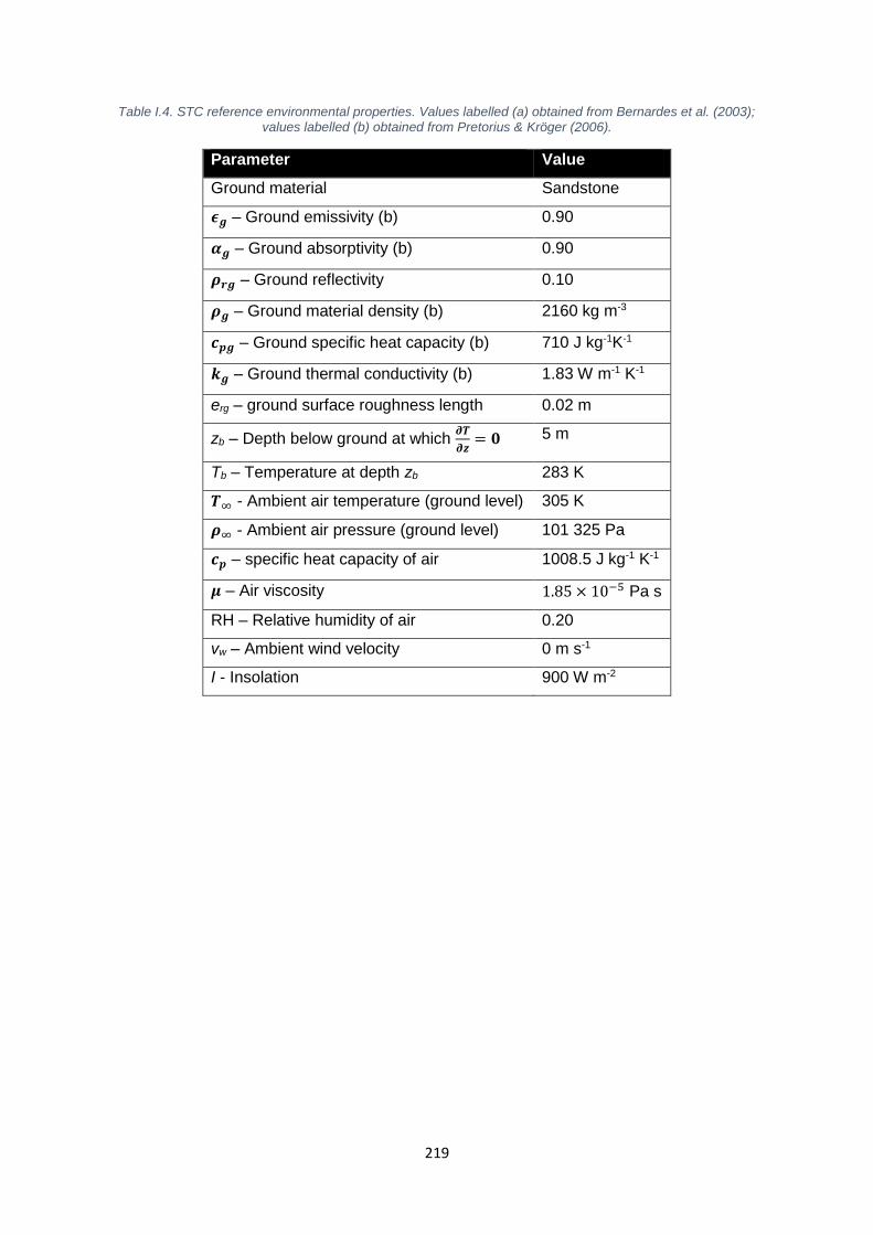
219
Table I.4. STC reference environmental properties. Values labelled (a) obtained from Bernardes et al. (2003); values labelled (b) obtained from Pretorius & Kröger (2006).
Parameter Value
Ground material Sandstone
𝝐𝒈 – Ground emissivity (b) 0.90
𝜶𝒈 – Ground absorptivity (b) 0.90
𝝆𝒓𝒈 – Ground reflectivity 0.10
𝝆𝒈 – Ground material density (b) 2160 kg m-3
𝒄𝒑𝒈 – Ground specific heat capacity (b) 710 J kg-1K-1
𝒌𝒈 – Ground thermal conductivity (b) 1.83 W m-1 K-1
erg – ground surface roughness length 0.02 m
zb – Depth below ground at which 𝝏𝑻
𝝏𝒛= 𝟎 5 m
Tb – Temperature at depth zb 283 K
𝑻∞ - Ambient air temperature (ground level) 305 K
𝝆∞ - Ambient air pressure (ground level) 101 325 Pa
𝒄𝒑 – specific heat capacity of air 1008.5 J kg-1 K-1
𝝁 – Air viscosity 1.85 × 10⁻⁵ Pa s
RH – Relative humidity of air 0.20
vw – Ambient wind velocity 0 m s-1
I - Insolation 900 W m-2

220
II. APPENDIX: STC NUMERICAL CHECKS
Rather than test STC performance across a range of component dimensions or
environmental conditions, this appendix has assessed STC performance for varying model
variables. For example, the model’s performance is examined across a range of collector
and chimney discretisation sizes; for a range of convergent stop criteria; and for a range of
initial assumed values when iteration is required.
The model parameters under study are given in Table II.1. Using the reference plant defined
in Appendix I, the model parameters detailed in Table II.1 are tested with a range of values
to establish model sensitivity to these parameters. Table II.2 validates the choice of STC
model parameters used in the reference plant. None of the parameters caused a variation in
power output by more than 4.2% from the selected reference STC model parameters. The
only parameter exhibiting a non-negligible dependence of the model on parameter value was
stop2, the convergence criterion for an iterative scheme to find the converged outlet air
temperature and velocity of each discretised collector section. Large values of stop2 result in
large differences between successive iterating foT values, and thus result in relatively large
changes in power output. Hence it is recommended that small values are selected for stop2.
Similarly, small values for r are beneficial (range in power outputs of 1.29%), but
excessively small values increase the model’s computational expense. Hence, a value of
2.0mr is recommended, except when simulating small STC power plants, where a
smaller r would be appropriate.
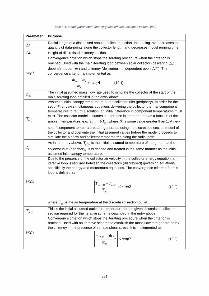
221
Table II.1. Model parameters (convergence criteria, assumed values, etc.)
Parameter Purpose
r Radial length of a discretised annular collector section. Increasing r decreases the
quantity of data-points along the collector length, and decreases model running time.
h Height of discretised chimney section.
stop1
Convergence criterion which stops the iterating procedure when the criterion is
reached. Used with the main iterating loop between solar collector (delivering T ,
dependent upon m ) and chimney (delivering m , dependent upon T ). The
convergence criterion is implemented as
1 1i i
i
m mstop
m
(12.1)
(1)m The initial assumed mass flow rate used to simulate the collector at the start of the
main iterating loop detailed in the entry above.
(1)cT
Assumed initial canopy temperature at the collector inlet (periphery). In order for the
set of First-Law simultaneous equations delivering the collector thermal component
temperatures to return a solution, an initial difference in component temperatures must
exist. The collector model assumes a difference in temperatures as a function of the
ambient temperature, e.g. (1)cT T , where is some value greater than 1. A new
set of component temperatures are generated using the discretised section model of
the collector and overwrite the initial assumed values before the model proceeds to
simulate the air flow and collector temperatures along the radial path.
(1)gT
As in the entry above, (1)gT is the initial assumed temperature of the ground at the
collector inlet (periphery). It is defined and treated in the same manner as the initial
assumed inlet canopy temperature.
stop2
Due to the presence of the collector air velocity in the collector energy equation, an
iterative loop is required between the collector’s (discretised) governing equations,
specifically the energy and momentum equations. The convergence criterion for this
loop is defined as
( 1) ( )
( )
2fo i fo i
fo i
T Tstop
T
(12.2)
where foT is the air temperature at the discretised section outlet.
(1)foT This is the initial assumed outlet air temperature for the given discretised collector
section required for the iterative scheme described in the entry above.
stop3
Convergence criterion which stops the iterating procedure when the criterion is
reached. Used with an iterative scheme to establish the mass flow rate generated by
the chimney in the presence of surface shear stress. It is implemented as
.
, 1 ,
,
3ch j ch j
ch j
m mstop
m
(12.3)
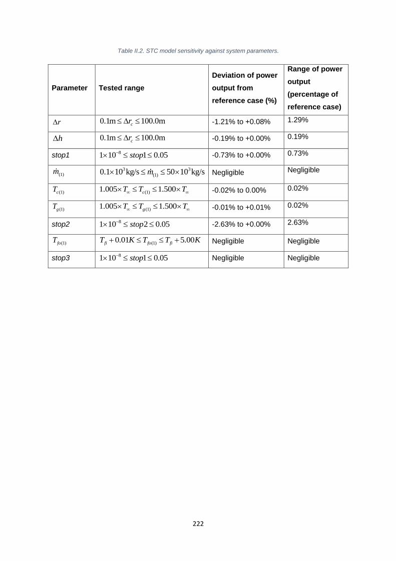
222
Table II.2. STC model sensitivity against system parameters.
Parameter Tested range
Deviation of power
output from
reference case (%)
Range of power
output
(percentage of
reference case)
r m 100.0m0.1 cr -1.21% to +0.08% 1.29%
h m 100.0m0.1 cr -0.19% to +0.00% 0.19%
stop1 810 1 0.051 stop -0.73% to +0.00% 0.73%
(1)m 3 3
(1)10 0 kg/s 50 10 kg.1 /sm Negligible Negligible
(1)cT (1)1.005 1.500cT T T -0.02% to 0.00% 0.02%
(1)gT (1)1.005 1.500gT T T -0.01% to +0.01% 0.02%
stop2 810 2 0.051 stop -2.63% to +0.00% 2.63%
(1)foT (1)0.01 5.00fi fo fiT K T T K Negligible Negligible
stop3 810 1 0.051 stop Negligible Negligible
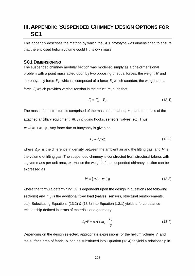
223
III. APPENDIX: SUSPENDED CHIMNEY DESIGN OPTIONS FOR
SC1
This appendix describes the method by which the SC1 prototype was dimensioned to ensure
that the enclosed helium volume could lift its own mass.
SC1 DIMENSIONING The suspended chimney modular section was modelled simply as a one-dimensional
problem with a point mass acted upon by two opposing unequal forces: the weight W and
the buoyancy force B
F , which is composed of a force W
F which counters the weight and a
force T
F which provides vertical tension in the structure, such that
.b W T
FF F (13.1)
The mass of the structure is comprised of the mass of the fabric, f
m , and the mass of the
attached ancillary equipment, xm , including hooks, sensors, valves, etc. Thus
f xW m gm . Any force due to buoyancy is given as
B
F Vg (13.2)
where is the difference in density between the ambient air and the lifting gas; and V is
the volume of lifting gas. The suspended chimney is constructed from structural fabrics with
a given mass per unit area, . Hence the weight of the suspended chimney section can be
expressed as
xW mA g (13.3)
where the formula determining A is dependent upon the design in question (see following
sections) and xm is the additional fixed load (valves, sensors, structural reinforcements,
etc). Substituting Equations (13.2) & (13.3) into Equation (13.1) yields a force balance
relationship defined in terms of materials and geometry:
T
x
FV A m
g (13.4)
Depending on the design selected, appropriate expressions for the helium volume V and
the surface area of fabric A can be substituted into Equation (13.4) to yield a relationship in
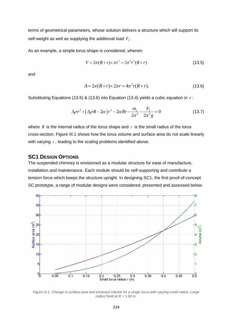
224
terms of geometrical parameters, whose solution delivers a structure which will support its
self-weight as well as supplying the additional load T
F .
As an example, a simple torus shape is considered, wherein
2 2 2
2 2( ) ( )V R r r r R r (13.5)
and
2(2 ) 2 4 ( ).R r r r R rA (13.6)
Substituting Equations (13.5) & (13.6) into Equation (13.4) yields a cubic equation in r :
3 2
2 22 2 0
2 2
x Tm F
r R Rr rg
(13.7)
where R is the internal radius of the torus shape and r is the small radius of the torus
cross-section. Figure III.1 shows how the torus volume and surface area do not scale linearly
with varying r , leading to the scaling problems identified above.
SC1 DESIGN OPTIONS The suspended chimney is envisioned as a modular structure for ease of manufacture,
installation and maintenance. Each module should be self-supporting and contribute a
tension force which keeps the structure upright. In designing SC1, the first proof-of-concept
SC prototype, a range of modular designs were considered, presented and assessed below.
Figure III.1. Change in surface area and enclosed volume for a single torus with varying small radius. Large
radius fixed at R = 1.00 m.

225
Table III.1. Properties common to all SC1 design options.
Parameter Value
Module height, h (Note h is an input variable for designs B & C, but an
output variable for design A ). 1.50 m
Internal radius, R . 0.25 m
Additional mass (valves, helium supply tubing, etc.), x
m . 0.100 kg
Tension force, F
T . 10 N
Density difference between air and helium, , calculated at 0K30T
and ambient pressure 1013 Pa25p . The helium gas is positively
pressurised to 400 Pa. Densities are calculated using the Ideal Gas law.
1.014
kgm-3
Specific mass of the fabric, . 0.026
kgm-2
To enable comparison across the different design schemes, the material properties and
internal radius were fixed, as shown in Table III.1. It was envisioned that the SC1 would
consist of two repeated fabric modules, with a total height below 4 m and a suitable
slenderness ratio such that it resembled a chimney and had the capacity to provide useful
structural behaviour data as a scaled model.
SC1A:
This design comprises two stacked tori per module, with the lower torus filled with
compressed air (see Figure III.2). In this initial design appraisal, and given the small
dimensions of the structure, it is assumed that the compressed air does not add weight to
the structure.
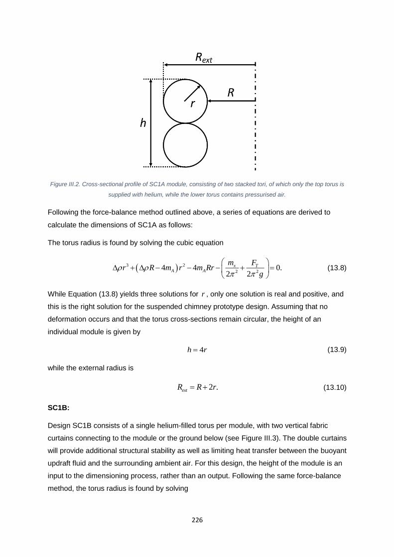
226
Figure III.2. Cross-sectional profile of SC1A module, consisting of two stacked tori, of which only the top torus is
supplied with helium, while the lower torus contains pressurised air.
Following the force-balance method outlined above, a series of equations are derived to
calculate the dimensions of SC1A as follows:
The torus radius is found by solving the cubic equation
3 2
2 24 4
20.
2
x TA A
m Fr R m m Rrr
g
(13.8)
While Equation (13.8) yields three solutions for r , only one solution is real and positive, and
this is the right solution for the suspended chimney prototype design. Assuming that no
deformation occurs and that the torus cross-sections remain circular, the height of an
individual module is given by
4h r (13.9)
while the external radius is
2 .ext R rR (13.10)
SC1B:
Design SC1B consists of a single helium-filled torus per module, with two vertical fabric
curtains connecting to the module or the ground below (see Figure III.3). The double curtains
will provide additional structural stability as well as limiting heat transfer between the buoyant
updraft fluid and the surrounding ambient air. For this design, the height of the module is an
input to the dimensioning process, rather than an output. Following the same force-balance
method, the torus radius is found by solving
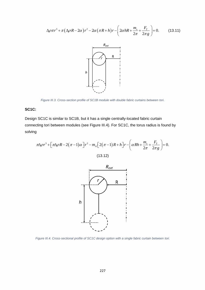
227
3 2 22 22 2
0.x Tm F
r R R hr r hRg
(13.11)
Figure III.3. Cross-section profile of SC1B module with double fabric curtains between tori.
SC1C:
Design SC1C is similar to SC1B, but it has a single centrally-located fabric curtain
connecting tori between modules (see Figure III.4). For SC1C, the torus radius is found by
solving
3 2 2 02 1 12
.2
x TAr R
m Fr R m Rhh
gr
(13.12)
Figure III.4. Cross-sectional profile of SC1C design option with a single fabric curtain between tori.

228
Design Comparison:
Using the design variables specified in Table III.1, the three proposed designs deliver
different design dimensions, as shown in Table III.2. Design SC1C marginally out-performs
designs SC1A and SC1B – it uses less fabric and consumes less helium. More importantly,
it has a smaller external radius, enabling it to achieve a more suitable slenderness ratio than
the other two designs. The slenderness ratio is defined as the ratio of the total chimney
diameter to the total chimney height (two modules), and slenderness ratios for all three
designs are given in Table III.3. Commercial chimneys would be expected to have a
slenderness ratio of no more than 0.2 (indicating a chimney five times as tall as it is wide). In
this test, lower slenderness ratios are better, and for this reason SC1C was selected for
manufacture.
The achieved slenderness ratios in the range 0.64 – 0.68 indicate the difficulty in designing
laboratory-scale suspended chimneys posed by the scaling issues identified above, even
when an exceptionally light fabric is used to minimise required lifting volume. A suspended
chimney module of the same height and internal radius utilising industry-standard fabrics (
-20.500kgmfm ) would have an external radius of 2.18 m (design option C), giving it a total
chimney slenderness ratio of 4.36 / 3.00 1.45 , or nearly 1.5 times as wide as it was tall.
Such a structure would not behave like a slender chimney under load and would not be
suitable for the proposed experiments, thus necessitating the use of the Octax helium-tight
film.
Table III.2. Dimensions and material consumption per module for all SC1 design options.
Design
Torus
radius,
r (m)
Module
height,
h (m)
External
radius,
extR (m)
He
volume,
V (m3)
Fabric
area, A
(m2)
A 0.36 1.44 0.97 1.55 17.24
B 0.37 1.50
(input) 0.98 1.63 20.52
C 0.34 1.50
(input) 0.94 1.39 11.10

229
Table III.3. SC1 design options - total chimney external dimensions.
Design External diameter
(m)
Total chimney
height (m) Slenderness ratio
A 1.94 1.44 0.674
B 1.96 1.50 0.653
C 1.92 1.50 0.640

230
IV. APPENDIX: SUSPENDED CHIMNEY DESIGN
PARAMETERS
Table IV.1. Suspended chimney parameters.
Parameter Symbol Parameter type Reference Values
Dimensions
Chimney inner radius 𝑟1 Independent 0.50 m
Inner sheath diameter 𝑑1 Independent 0.20 m
Helium torus cell diameter 𝑑2 Dependent 2.54 m
Outer sheath diameter 𝑑3 Independent 0.20 m
Cell height ℎ Independent 10.00 m
Number of formers inside inner sheath
𝑛1 Independent 16
Proportion of inner sheath’s former sheets retaining material
𝑓1 Independent 0.80
Number of formers inside outer sheath
𝑛3 Independent 32
Proportion of outer sheath’s former sheets retaining material
𝑓3 Independent 0.80
Fabric surface area - inner sheath 𝐴1 Dependent 58 m2
Fabric surface area - helium cell 𝐴2 Dependent 310 m2
Fabric surface area - outer sheath 𝐴3 Dependent 272 m2
Volume - inner sheath 𝑉1 Dependent
Volume - Helium cell 𝑉2 Dependent 314 m3
Volume - Outer sheath 𝑉3 Dependent
Materials
Inner sheath material specific weight 𝛼1 Independent 0.120 kgm-2
Helium cell material specific weight 𝛼2 Independent 0.420 kgm-2
Outer sheath material specific weight
𝛼3 Independent 0.120 kgm-2
Gas Parameters
Inner sheath air gauge pressure 𝑝1 Independent 10 kPa
Helium cell gauge pressure 𝑝2 Independent 400 Pa
Outer sheath air gauge pressure 𝑝3 Independent 10 kPa
Helium purity ratio (by volume) 𝛾 Independent; 1.0 = 100% helium; 0.0 = 100% air
0.99
Gas temperature 𝑇 Environmental 300 K
Ambient pressure (absolute) 𝑝𝑎 Environmental 101325 Pa
Specific gas constant – air 𝑅𝑎 Constant 287 Jkg-1K-1
Specific gas constant - helium 𝑅𝐻𝑒 Constant 2077 Jkg-1K-1
Loads and Masses
Mass of fabric – inner sheath 𝑚𝑓1 Dependent 7.03 kg
Mass of fabric – Helium cell 𝑚𝑓2 Dependent 130.21 kg
Mass of fabric – outer sheath 𝑚𝑓3 Dependent 32.67 kg
“Dead” mass per cell 𝑚𝑥 Independent 40 kg
Total mass of cell 𝑚𝑠 Dependent 431.29 kg
Buoyancy force of cell 𝐹𝑏 Dependent 3090 N
Tension force in cell 𝐹𝑇 Independent 400 N

231
V. APPENDIX: DERIVATION OF SC2 DIMENSIONING
EQUATION
This appendix provides the mathematical derivation of the quadratic equation which enables
the specification of the helium-filled wall thickness.
The dimensions of the cell can be determined with a simple force balance,
,b TF mg F (15.1)
in which the buoyancy force term expands as
2 2( ) ,b aF V g (15.2)
and the mass term expands as
1 1 1 1 2 2 3 3 3 3( .) ( )a a xm V A mA A V (15.3)
Each of the area and volume terms are defined by the dimensional parameters as identified
in Figure 7.12 and Table IV.1.
The parameters of Equation (15.3) are given as follows:
Surface area of the inner air-filled sheath:
2
1 1 12 ( ) 2r h dA d (15.4)
Volume of the inner air-filled sheath:
1 1 1(2 )hV d r d (15.5)
Surface area of the helium cell:
2
2 2 1 2 12 2( ) 4 ( )2 hd h d r dA d r h (15.6)
Volume of the helium cell:
2
2 2 1 22 ( )hd h d r dV (15.7)
Surface area of the outer air-filled sheath:
3 3 2 3 1 3 1( 2 ) 2 )2 ( 2 ( )h d d d d r h dA d r (15.8)

232
Volume of the outer air-filled sheath:
3 3 2 3 3 12 2( )hd d h rV dd d (15.9)
Substituting Eqs (15.2) - (15.9) into Eq (15.1) and rearranging to form a quadratic in 2d , we
obtain
2
2 2 2
2 3 3 3 3 2 1 2
1 1 1 3 3 3 3
1 1 2 1 1 3 3 3 1
)
2 ) (2 ) (2 )( )
( 2 ) ( 2
(2
(
)
( 4 2 2 2 )( ) 0x T
hd
h h d h d r
d rh d d h
m Fd h h
d
d d h hd r dg
(15.10)
where 1 1 a ; 2 2a ; and 3 3 a . Note that in this formulation the
order of the densities is reversed for the helium cell (subscript 2) to ensure that the
terms always remain positive. For the lighter-than-air gas envelope, which contains a mixture
of lighter-than-air gas (subscript g) and ambient air (subscript ∞), 2 is calculated according
to the Ideal Gas Law as
2
2 22 ,
11
g
p p
T R
p
R
(15.11)
where is the proportion (by volume) of the lifting volume filled by lighter-than-air gas. This
factor is included as even small amounts of non-lifting gas in the lifting volume can have a
significant impact upon the buoyancy force generated. In this analysis, it is assumed that any
non-lifting gas has the same properties as air. It is assumed that the gas mixture is
isothermal and in thermal equilibrium with the ambient air.
Note also that Equation (15.11) accommodates the pressure difference between the ambient
air (subscript ∞) and the gas mixture within the envelope (subscript 2). The lighter-than-air
gas envelope will be maintained above ambient pressure to maintain the structure’s shape
only. Structural stiffness is provided by the pressurised air-filled sheathes (subscript 1 and
3), which will be maintained significantly above ambient pressure. As such, the density
difference between the air-filled sheathes and the ambient is found using
,p p
R T
(15.12)

233
where the density and pressure terms without subscript belong to the pressurised air
sheathes (either inner or outer), and the properties with subscript ∞ denote ambient air
values.

234
VI. APPENDIX: SUSPENDED CHIMNEY DESIGN DRAWINGS
– 20 M TALL
When inflated, the structure will have a ridged appearance, as the air pressure causes the
fabric to bow between the formers. The drawings include all the technical parameters
supplied as inputs to the suspended chimney dimensioning model, and represent the
dimensions of this suspended chimney design applied to a structure constructed from two
modules each 10 m tall.
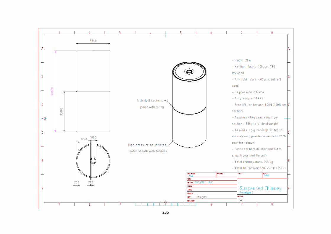
235

236

237
VII. APPENDIX: SC2 PROTOTYPE DESIGN

238
VIII. APPENDIX: SC PROTOTYPES – 20 M TALL – DESIGN OPTIONS
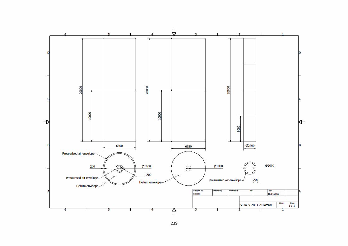
239
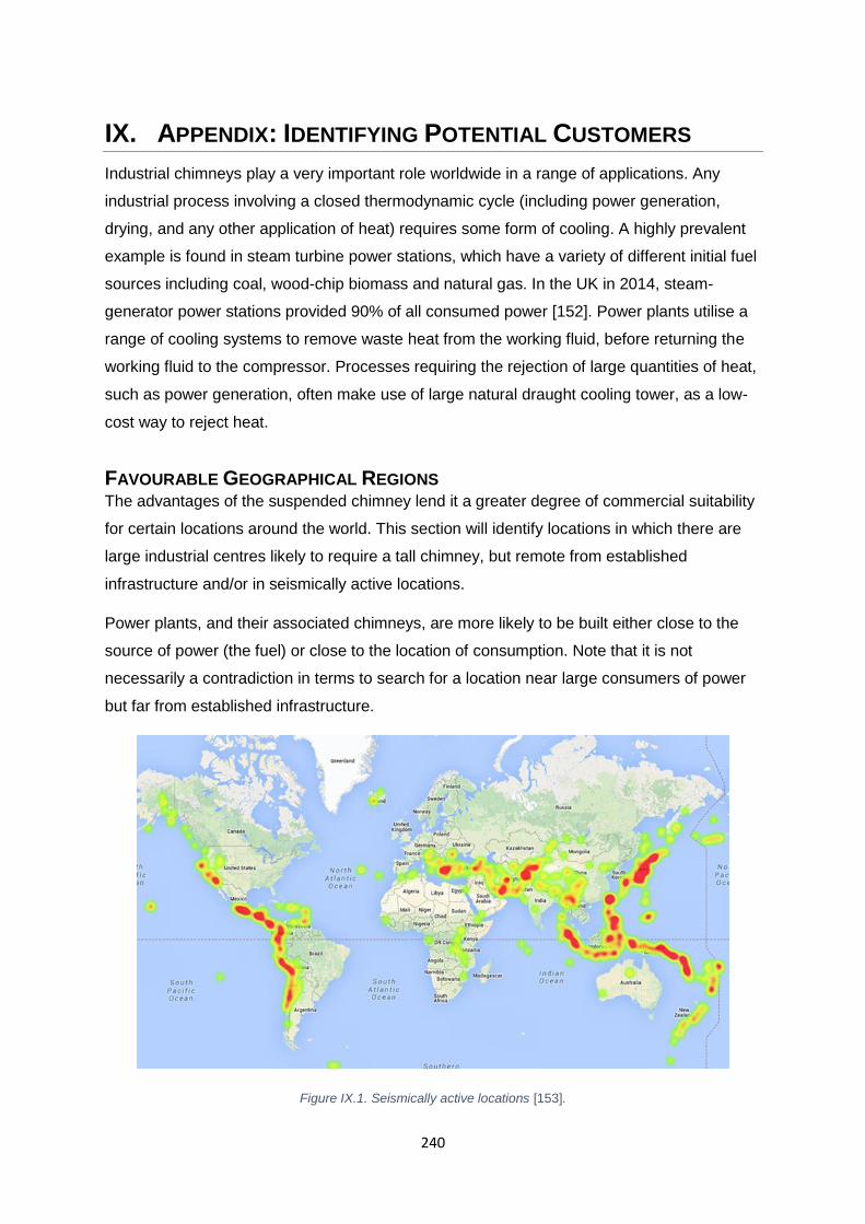
240
IX. APPENDIX: IDENTIFYING POTENTIAL CUSTOMERS
Industrial chimneys play a very important role worldwide in a range of applications. Any
industrial process involving a closed thermodynamic cycle (including power generation,
drying, and any other application of heat) requires some form of cooling. A highly prevalent
example is found in steam turbine power stations, which have a variety of different initial fuel
sources including coal, wood-chip biomass and natural gas. In the UK in 2014, steam-
generator power stations provided 90% of all consumed power [152]. Power plants utilise a
range of cooling systems to remove waste heat from the working fluid, before returning the
working fluid to the compressor. Processes requiring the rejection of large quantities of heat,
such as power generation, often make use of large natural draught cooling tower, as a low-
cost way to reject heat.
FAVOURABLE GEOGRAPHICAL REGIONS The advantages of the suspended chimney lend it a greater degree of commercial suitability
for certain locations around the world. This section will identify locations in which there are
large industrial centres likely to require a tall chimney, but remote from established
infrastructure and/or in seismically active locations.
Power plants, and their associated chimneys, are more likely to be built either close to the
source of power (the fuel) or close to the location of consumption. Note that it is not
necessarily a contradiction in terms to search for a location near large consumers of power
but far from established infrastructure.
Figure IX.1. Seismically active locations [153].

241
An example of such would be the Atacama Desert in Chile, where substantial mining and
scientific operations take place, but which is located far from Chile’s national power
infrastructure. Seismically active locations are shown in Figure IX.1. A shortlist of locations
near fuel sources or consumption centres, far from established infrastructure and/or in a
seismically active region have been drawn up below:
• Atacama Desert, Chile: As recorded above, the Atacama Desert is a consumption
centre due to the presence of heavy industry, but its remote location makes
infrastructure connection difficult, and thus it would suit the reduced transport
requirements of the suspended chimney.
• California, Nevada & Arizona, USA: Home to several major cities including Los
Angeles, San Francisco, and Las Vegas, this region has several consumption
centres. It also suffers large earthquakes due to the neighbouring San Andreas fault.
• New Zealand: The entire country suffers earthquakes. The most recent was a large
earthquake which struck in November 2016 measuring 7.8 on the Richter Scale. The
most devastating recent quake struck in February 2011, causing great damage and
loss of life in Christchurch, New Zealand’s third largest city.
• Central China: Mining and other economic activity has developed rapidly in Central
China over the preceding two decades. National power and transport infrastructure is
minimal, and locations not capable of producing their own building materials for the
chimney would benefit from the reduced transportation load offered by the
suspended chimney.
CHARACTERISATION OF POTENTIAL CUSTOMERS The suspended chimney can be deployed in any scenario in which a conventional chimney
may be required, making it suitable for a wide range of uses. Commercial activity will fund
further research and development to ensure that the suspended chimney meets all
necessary standards which will be required by potential customers, in terms of fire
retardation and fabric material protection against the gases and particulates vented through
the SC. Despite robust plans for research and development, suspended chimney
performance in commercial industrial settings cannot be predicted with complete accuracy.
As such, the profile of initial customers should be defined in order to procure and establish
relationships with suitable candidates. The initial customers for each commercial suspended
chimney (of increasing sizes) should be technically-literate early adopters with an interest in
innovation and an understanding of the risks involved in making step changes compared to
incremental improvements. In order to ensure the success of the suspended chimney
product, the development company’s engineers would require regular access to the first

242
commercial units in their operating environment to assess and improve their performance,
both for existing units under operation and future units yet to be sold. It would be especially
advantageous to equip the first commercial SCs with full instrumentation similar to the
prototype SCs, in order to fully analyse the commercial SCs performance in their operating
environment.
Customer engagement for the first commercial SCs is essential to address any issues which
may arise. As such, these customers should be carefully selected and relationships with
them should be cultivated from the earliest opportunity, with a tone of partnership as much
as customer and supplier. The nature of their operations and the impact of any adverse
event originating from the SC upon their profitability should also be taken into account.
243
X. APPENDIX: COMMERCIAL SUSPENDED CHIMNEY COSTS
This appendix provides large-scale suspended chimney sizes and cost forecasts to assess
the viability of the suspended chimney innovation at commercial scale, as would be required
for the solar thermal chimney power plant.
Properties and dimensions common to all designs are:
• Helium-envelope fabric:
o Density: 0.400 kg/m2
o Cost: £14.17/m2.
• Additional dead mass: 1.00 kg per metre height.
• Helium cost: £7.70/m3 plus transport & rental of equipment.
• Manufacturing:
o Manufacturing time at Lindstrand Technologies: 40 hours per metre height.
o Manufacturing cost: £45 / hour.
Currently, the designs under analysis all assume no additional stiffening nor tension in the
fabric structure. Each design is neutrally buoyant without additional resistance to lateral load.
The design in question is the simple double-walled chimney, with helium filling the void
between the walls. Fabric formers are included to ensure that the fabric maintains its shape.
The additional mass accounts for extra fabric used in the welding process, for valves and
pipework and for the mass of joining methods between the sections. Table X.1 presents the
forecast dimensions and costs for all configurations, including data which was deemed non-
essential in the body of the report.
Throughout the main body of the thesis, all costs are expressed in US dollars, using a
conversion rate of £1 = $1.34.

244
Table X.1. Forecast commercial-scale suspended chimney dimensions and costs (comprehensive version).
Chimney Design SC7 SC8 SC9 SC10 SC11
Total height (m)
100 300 500 1000 1000
Internal diameter (m)
5 15 25 50 110
Internal ratio 0.05 0.05 0.05 0.05 0.11
Quantity of sections 5 15 20 40 40
Section height (m)
20 20 25 25 25
Additional non-lifting mass
(kg) 100 300 500 1000 1000
Quantity of former sheets
24 36 50 100 100
Proportion of former sheets retained
1 1 1 1 1
He wall width (m)
1.76 1.23 1.12 1.11 0.93
External diameter (m)
8.52 17.46 27.24 52.22 111.86
External ratio 0.085 0.058 0.054 0.052 0.112
Total fabric area (m2)
4436 31532 83901 328277 709964
Total chimney mass (kg)
1874 12913 34060 132311 284986
Total He consumption
(m3, STP) 3743 18803 45993 178412 324208
Lead time (years)
2.08 6.25 10.42 20.83 20.83
Estimated material cost
(£) £ 62,809 £ 446,487 £ 1,188,039 £4,648,403 £10,053,089
Estimated labour cost
(£) £180,000 £ 540,000 £ 900,000 £1,800,000 £ 1,800,000
Estimated He cost (£, single inflation)
£ 29,478 £ 145,981 £ 356,247 £1,377,969 £ 2,504,499
Estimated total cost (£, to 1st inflation)
£272,287 £ 1,132,468 £ 2,444,287 £7,826,372 £14,357,589
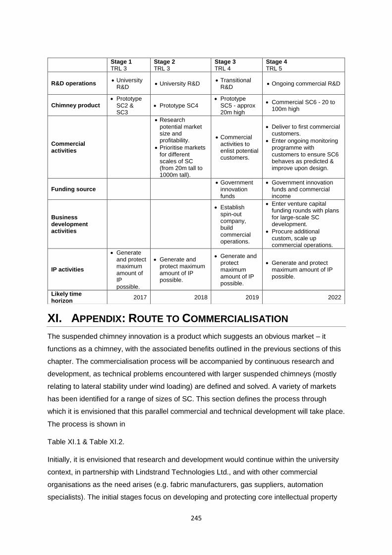
245
XI. APPENDIX: ROUTE TO COMMERCIALISATION
The suspended chimney innovation is a product which suggests an obvious market – it
functions as a chimney, with the associated benefits outlined in the previous sections of this
chapter. The commercialisation process will be accompanied by continuous research and
development, as technical problems encountered with larger suspended chimneys (mostly
relating to lateral stability under wind loading) are defined and solved. A variety of markets
has been identified for a range of sizes of SC. This section defines the process through
which it is envisioned that this parallel commercial and technical development will take place.
The process is shown in
Table XI.1 & Table XI.2.
Initially, it is envisioned that research and development would continue within the university
context, in partnership with Lindstrand Technologies Ltd., and with other commercial
organisations as the need arises (e.g. fabric manufacturers, gas suppliers, automation
specialists). The initial stages focus on developing and protecting core intellectual property
Stage 1 TRL 3
Stage 2 TRL 3
Stage 3 TRL 4
Stage 4 TRL 5
R&D operations • University
R&D • University R&D
• Transitional R&D
• Ongoing commercial R&D
Chimney product • Prototype
SC2 & SC3
• Prototype SC4 • Prototype
SC5 - approx 20m high
• Commercial SC6 - 20 to 100m high
Commercial activities
• Research potential market size and profitability.
• Prioritise markets for different scales of SC (from 20m tall to 1000m tall).
• Commercial activities to enlist potential customers.
• Deliver to first commercial customers.
• Enter ongoing monitoring programme with customers to ensure SC6 behaves as predicted & improve upon design.
Funding source • Government
innovation funds
• Government innovation funds and commercial income
Business development activities
• Establish spin-out company, build commercial operations.
• Enter venture capital funding rounds with plans for large-scale SC development.
• Procure additional custom, scale up commercial operations.
IP activities
• Generate and protect maximum amount of IP possible.
• Generate and protect maximum amount of IP possible.
• Generate and protect maximum amount of IP possible.
• Generate and protect maximum amount of IP possible.
Likely time horizon
2017 2018 2019 2022
246
on which the suspended chimney product is based. This includes manufacturing and testing
further prototypes, at a scale of 20 m tall and larger. Funding will be sought from grant-
making bodies supporting research and innovation, such as the EPSRC and the Royal
Society, or in response to calls by the EU’s Horizon 2020, if UK-based projects remain
eligible.
At the same time, commercial activities will begin to develop, including founding a spin-out
company to commercialise the SC product and procuring initial customer-partners for whom
the very first commercial SCs can be installed, fully instrumented, to ensure their
performance in an industrial setting. The performance data from these SCs will be analysed
and the manufacturing methods re-appraised to identify potential improvements and cost-
saving changes. This process will continue on a larger scale, with commercial income and
venture capital funding the development of larger SCs, which will in turn be introduced to the
market in the same manner. Eventually, SCs capable of standing greater than 500m tall will
be developed for use within a solar thermal chimney power plant, delivering large quantities
of renewable base-load power and providing a dependable long-term income. The
development of such large SC structures is a long-term goal, requiring several viable
markets for smaller SCs to support development. Such markets also ensure that the
enterprise remains profitable should the development of exceptionally large SCs eventually
prove unsuccessful.
Potential exit strategies include selling the STC operations contracts once multiple STCs are
installed and generating power. Large-scale renewable power producers can attract extra
subsidies or price guarantees for the power they produce, making their owners and
operators attractive as low-risk profitable enterprises. The quantity of IP generated
throughout this process is expected to be substantial, and all options including licensing and
sale of the IP will be considered in due course. The future IP generated may also lend itself
to different innovative products, all of which will be considered and commercialised if
deemed viable. Strong ties to universities and grant-making innovation support organisations
will be maintained for this to be accomplished in a cost-effective manner.
HIRE OF SUSPENDED CHIMNEYS Revenue generation can be achieved by selling and maintaining suspended chimneys.
However, other business models are possible, including that of the rapid-response
replacement chimney for industrial plants. Many industrial plants rely on their chimneys for
active thermodynamic cooling or exhausting waste gases safely, and cannot operate without
the chimney structure. If an industrial plant’s conventional chimney(s) are unable to fulfil their
function for any reason – including earthquakes, the discovery of structural issues, or routine

247
maintenance – a suspended chimney can be delivered and installed at short notice, enabling
the plant to continue operating. Potential customers include owners and operators of power
stations, who often have contracts with their customers which impose penalties if their
generation availability drops below agreed levels.
The SC’s modular design means multiple chimney configurations can be catered for with the
same SC modules. Revenue can be generated by hiring out the suspended chimney, as
may suit an industrial plant carrying out planned maintenance on their conventional chimney
structures; or by selling chimney insurance products, in which the industrial plant’s operators
pay a regular premium to minimise down-time in the event of an unexpected chimney failure.
Providing the SC can be installed and made operational sufficiently quickly, the cost of hiring
an SC or “insuring” their current conventional structures with on-demand temporary SC
replacements will be small compared to the cost of ceasing plant operation. Large scale
power plants and their operating companies are considered to be good potential customers
for the SC-as-insurance option.

248
Table XI.1. SC route to commercialisation - Stages 1 - 4.
Stage 1 TRL 3
Stage 2 TRL 3
Stage 3 TRL 4
Stage 4 TRL 5
R&D operations • University
R&D • University R&D
• Transitional R&D
• Ongoing commercial R&D
Chimney product • Prototype
SC2 & SC3
• Prototype SC4 • Prototype
SC5 - approx 20m high
• Commercial SC6 - 20 to 100m high
Commercial activities
• Research potential market size and profitability.
• Prioritise markets for different scales of SC (from 20m tall to 1000m tall).
• Commercial activities to enlist potential customers.
• Deliver to first commercial customers.
• Enter ongoing monitoring programme with customers to ensure SC6 behaves as predicted & improve upon design.
Funding source • Government
innovation funds
• Government innovation funds and commercial income
Business development activities
• Establish spin-out company, build commercial operations.
• Enter venture capital funding rounds with plans for large-scale SC development.
• Procure additional custom, scale up commercial operations.
IP activities
• Generate and protect maximum amount of IP possible.
• Generate and protect maximum amount of IP possible.
• Generate and protect maximum amount of IP possible.
• Generate and protect maximum amount of IP possible.
Likely time horizon
2017 2018 2019 2022
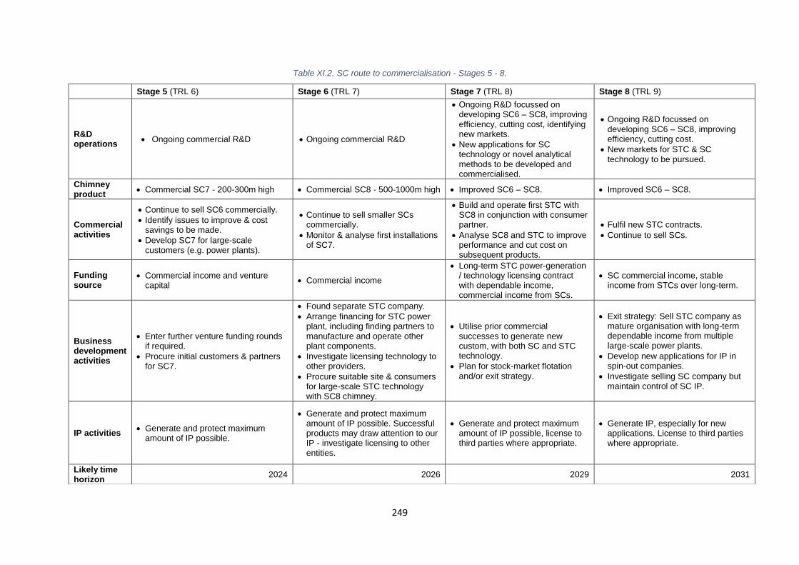
249
Table XI.2. SC route to commercialisation - Stages 5 - 8.
Stage 5 (TRL 6) Stage 6 (TRL 7) Stage 7 (TRL 8) Stage 8 (TRL 9)
R&D operations
• Ongoing commercial R&D • Ongoing commercial R&D
• Ongoing R&D focussed on developing SC6 – SC8, improving efficiency, cutting cost, identifying new markets.
• New applications for SC technology or novel analytical methods to be developed and commercialised.
• Ongoing R&D focussed on developing SC6 – SC8, improving efficiency, cutting cost.
• New markets for STC & SC technology to be pursued.
Chimney product
• Commercial SC7 - 200-300m high • Commercial SC8 - 500-1000m high • Improved SC6 – SC8. • Improved SC6 – SC8.
Commercial activities
• Continue to sell SC6 commercially.
• Identify issues to improve & cost savings to be made.
• Develop SC7 for large-scale customers (e.g. power plants).
• Continue to sell smaller SCs commercially.
• Monitor & analyse first installations of SC7.
• Build and operate first STC with SC8 in conjunction with consumer partner.
• Analyse SC8 and STC to improve performance and cut cost on subsequent products.
• Fulfil new STC contracts.
• Continue to sell SCs.
Funding source
• Commercial income and venture capital
• Commercial income
• Long-term STC power-generation / technology licensing contract with dependable income, commercial income from SCs.
• SC commercial income, stable income from STCs over long-term.
Business development activities
• Enter further venture funding rounds if required.
• Procure initial customers & partners for SC7.
• Found separate STC company.
• Arrange financing for STC power plant, including finding partners to manufacture and operate other plant components.
• Investigate licensing technology to other providers.
• Procure suitable site & consumers for large-scale STC technology with SC8 chimney.
• Utilise prior commercial successes to generate new custom, with both SC and STC technology.
• Plan for stock-market flotation and/or exit strategy.
• Exit strategy: Sell STC company as mature organisation with long-term dependable income from multiple large-scale power plants.
• Develop new applications for IP in spin-out companies.
• Investigate selling SC company but maintain control of SC IP.
IP activities • Generate and protect maximum
amount of IP possible.
• Generate and protect maximum amount of IP possible. Successful products may draw attention to our IP - investigate licensing to other entities.
• Generate and protect maximum amount of IP possible, license to third parties where appropriate.
• Generate IP, especially for new applications. License to third parties where appropriate.
Likely time horizon
2024 2026 2029 2031


![Literatur 26022019 test - TU Braunschweig · 2015 [1] Aizpurua Aldasoro, H.: On Gust Buffeting Design of Slender Chimneys – Building Interference and Fatigue. Dissertation April](https://static.cupdf.com/doc/110x72/6068ec4d422fa2738f4f4587/literatur-26022019-test-tu-braunschweig-2015-1-aizpurua-aldasoro-h-on-gust.jpg)