Informed Trading and Expected Returns
James J. Choi Yale School of Management and NBER
Li Jin
Oxford University Saïd Business School and Peking University Guanghua School of Management
Hongjun Yan
Rutgers Business School
May 14, 2016
Abstract
Does information asymmetry affect the cross-section of expected stock returns? We explore this
question using representative portfolio holdings data from the Shanghai Stock Exchange. We
show that institutional investors have a strong information advantage, and that past
aggressiveness of institutional trading in a stock positively predicts institutions’ future
information advantage in this stock. Sorting stocks on this predictor and controlling for other
correlates of expected returns, we find that the top quintile’s average annualized return in the
next month is 10.8% higher than the bottom quintile’s, indicating that information asymmetry
increases expected returns.
We thank Jennifer Carpenter, Jia Chen, Bryan Kelly, Alexander Ljunqvist, Roger Loh, Jialin Yu, and audience members at ABFER, Brigham Young University, Brown, Cheung Kong GSB, CICF, EFA, Hong Kong University, HKUST, INSEAD, NYU, the SEC, SUNY Binghamton, University of Rochester, University of Toronto, and Yale for their insightful comments. [email protected] (203-436-1833), [email protected], [email protected].
1
Does information asymmetry affect the cross-section of expected stock returns? The
theoretical literature has come to different conclusions. Easley and O’Hara (2004) argue that
stocks with more information asymmetry should have higher expected returns to compensate
uninformed investors for the losses they suffer from trading against informed investors. Their
model shows that, holding the total quantity of information constant, stocks with more private
information have a higher return premium. However, Hughes, Liu, and Liu (2007) argue that the
relationship between information asymmetry and expected returns disappears in large economies
because of diversification. Lambert, Leuz, and Verrecchia (2011) argue that, holding the average
precision of investors’ beliefs about a stock’s fundamental value constant, a positive relationship
between information asymmetry and expected returns arises only in financial markets where
investors are not price-takers. Models with only one risky asset provide intuitions that
information asymmetry might affect the cross-section of expected returns through its effects on
liquidity, the usefulness of an asset for risk-sharing, and the risk-bearing capacity available
through market makers, but the sign of the predicted relationship differs both within and across
models (Diamond and Verrecchia (1991), Gârleanu and Pedersen (2004), Vayanos and Wang
(2012)).
Empirical tests of the cross-sectional relationship between information asymmetry and
expected returns have to overcome the difficulty of identifying stock-level variation in
information asymmetry.1 In this paper, we identify stock-level information asymmetry using a
unique dataset that contains the daily stock holdings of a representative sample of all Shanghai
Stock Exchange investors. Our setup is appealing for several reasons. First, the high frequency
and representative nature of our sample allows us to more accurately measure the prevalence of
informed trading than in most other markets, where ownership data are either available only at
much lower frequencies or come from a non-representative investor sample. Second, due to the
less-developed state of Chinese legal institutions and regulations, there is likely to be greater
cross-sectional variation in how much private information is shared with selected investors than
in developed markets, where a stricter regulatory environment compresses the amount of
information asymmetry among active traders towards zero. This greater variation gives our
1 See Cornell and Sirri (1992), Neal and Wheatley (1998), Van Ness, Van Ness, and Warr (2001), and Collin-Dufresne and Fos (2015) for evidence that measures of adverse selection derived from liquidity measures do a poor job of measuring information asymmetry.

2
analysis more statistical power to detect information asymmetry effects on expected returns.
Finally, Chinese stock returns share many features of developed market stock returns—for
example, during our sample period, market capitalization, book-to-market ratios, and past-year
returns predict future returns in the Shanghai Stock Exchange—suggesting that return
phenomena in China offer insights into returns in other markets as well. Carpenter, Lu, and
Whitelaw (2015) conclude that “Chinese investors price risk and other stock characteristics
remarkably like investors in other large economies.”2 They also find that notwithstanding the
market’s reputation as a casino, “the average level of stock price informativeness [for future
corporate earnings] in China over the period [1996 to 2012] is similar to that in the US.”
We use the collective actions of one group of informed investors to create a proxy for the
general amount of information asymmetry in a stock. The investors we focus on are institutions,
which we demonstrate have a large information advantage in the Shanghai Stock Exchange. If
each week during our 1996 to 2007 sample period, one bought stocks whose log institutional
ownership percentage change in the prior week was in the top quintile and sold short stocks
whose log institutional ownership percentage change in the prior week was in the bottom
quintile, the resulting four-factor portfolio alpha was 144 basis points per month, or 17.3% per
year, and significant at the 0.1% level (t = 5.62).3
Stocks in which institutions collectively have a greater information advantage are stocks
that we classify as having more information asymmetry. In both the monopolistic setting of Kyle
(1985) and the competitive setting of Easley and O’Hara (2004), informed trader expected profits
are increasing in his/their information advantage. A naïve approach to estimating the effect of
information asymmetry on expected returns is to regress realized abnormal stock returns from
time t to t + 1 on the (eventually) realized profits of institutional trades initiated in the stock
during t. The problem with this approach is that realized profits are the sum of expected profits—
the variable whose effect we are interested in—and realized noise. Realized noise in profits may
2 Chen et al. (2010) test 18 variables that have been shown to predict the cross section of stock returns in the U.S. market and find that in the 1995 to 2007 period, all 18 variables’ point estimates in univariate Fama-MacBeth (1973) regressions have signs consistent with the U.S. evidence, and five are statistically significant, compared to eight significant coefficients for the U.S. markets during this same period. 3 During our sample period, short sales were prohibited in China. The “long-short returns” should be interpreted as return differences rather than trading profits.

3
be correlated with contemporaneously realized noise in the stock’s return, creating estimation
bias that is not merely an attenuation towards zero.
The empirical strategy we adopt instead is to find an ex ante predictor of institutional
trading profits and hence information asymmetry. By constructing the predictor using only
information available at t, we make it uncorrelated with realized noise in both trading profits and
returns that occur after t. We then estimate the relationship between this predictor and expected
returns.
Our predictor of information asymmetry is the aggressiveness with which institutions
have previously traded in the stock, as measured by the average of the 50 most recent weekly
absolute institutional ownership percentage changes in the stock.4 Our “prior institutional
ownership volatility” variable is motivated by the intuition that institutions’ trades in stocks
where they have no information advantage are primarily caused by their need to invest customer
asset inflows, rebalance, and meet liquidity demands, whereas institutional trades in stocks
where they have an information advantage are additionally driven by value signals. Therefore,
institutional ownership volatility should be higher in stocks where institutions have a greater
information advantage.
We first confirm that in accordance with the above intuition, prior institutional ownership
volatility predicts institutions’ average weekly trading profit in a stock during the following
month.5 We then conduct our main cross-sectional return test. Consistent with information
asymmetry increasing expected returns, we find that stocks in the top quintile of prior
institutional ownership volatility as of month τ have an average return in month τ + 1 that is 90
basis points higher (10.8% annualized) than that of their bottom-quintile counterparts after
4 We have also tried using the past year’s institutional trading profits (as defined later in this paper) in a stock as a predictor of information asymmetry. The results of this alternative analysis are consistent with those reported in the paper: portfolios with higher predicted information asymmetry have higher future alphas in the cross-section. We do not use past trading profits as our main predictor because its relationship with current and future information asymmetry is non-monotonic—both stocks with very high and very low past institutional trading profits have higher information asymmetry than stocks with moderate past institutional trading profits—making the use of this variable expositionally inconvenient. Intuitively, if an investor has more precise information about a stock, she will on average make a more aggressive trade in the stock, and her realized trading profit will tend to be either very high or very low. 5 Our measure does not capture trading profits by informed individuals. Our proxy for information asymmetry will give directionally correct results if the information advantage that informed individuals have is not too negatively correlated with the information advantage of institutions.
4
controlling for size, book-to-market, and momentum effects, a difference that is significant at the
0.1% level (t = 3.51).
We present three pieces of evidence that the relationship between prior institutional
ownership volatility and expected returns is driven by information asymmetry, rather than some
unobserved factor. First, when we examine the results separately by market capitalization tercile,
we find that prior institutional ownership volatility predicts cross-sectional variation in current
and future institutional trading profits only among large and mid-cap stocks, not among small
stocks. This does not mean that institutions have no information advantage in small stocks. In
fact, we find that institutions have a large information advantage in all size terciles. Rather, the
null result indicates that sorting on prior institutional ownership volatility creates no cross-
sectional variation in current and future institutional information advantage among small stocks.6
This provides a useful falsification test: If prior institutional ownership volatility is correlated
with expected returns only through the information asymmetry channel, then it should be
unrelated to expected returns among small stocks, while it should be related to expected returns
among large and mid-cap stocks. Indeed, we find that there is no significant four-factor alpha
difference (t = 0.45, p = 0.655) between the top and bottom quintiles of prior institutional
ownership volatility among small stocks. In contrast, the annualized four-factor alpha difference
between the extreme quintiles is 12.4% among mid-cap stocks (t = 3.39, p = 0.001) and 17.4%
among large-cap stocks (t = 3.56, p = 0.001).
Second, we examine how closely the persistence of institutional ownership volatility’s
ability to predict information asymmetry matches the persistence of its ability to predict expected
returns. If, for example, institutional ownership volatility’s month t value only predicted
variation in information asymmetry through month t + 1 but predicted variation in expected
returns through month t + 12, then its relationship with expected returns is probably operating
through some channel other than information asymmetry. We find that the differences in
information asymmetry across institutional ownership volatility quintiles formed in month t
persist until month t + 10, and so do the differences in expected returns. This is exactly what we
6 The lack of correlation between prior institutional ownership volatility and information asymmetry could be due to there being little variation in the degree of information asymmetry across small stocks, causing the variation in prior institutional ownership volatility in small stocks to be mostly driven by non-informational factors. Alternatively, institutions’ information advantage in any given small stock may be quite transitory, so that past trading behavior in a small stock gives little information about current and future information advantage in that stock.
5
would expect if our predictor is correlated with expected returns only because of its correlation
with information asymmetry.
Third, we rule out a number of alternative interpretations of the relationship between our
predictor and expected returns. We find that liquidity and price pressure from future institutional
buys and sells are not responsible for our main results. In fact, stocks in the top quintile of prior
institutional ownership volatility are more liquid and experience less institutional buying during
the month after portfolio formation than stocks in the bottom quintile, both of which act to lower
the top quintile’s returns. In addition, controlling for the generic non-information-related
propensity for institutions to hold each stock has no impact on the results.
The empirical literature that tries to identify the impact of information asymmetry on
expected returns has been controversial. Easley, Hvidkjaer, and O’Hara (2002) use the temporal
clustering of buy and sell orders to estimate the probability of informed trading (PIN) and find
that high-PIN stocks have higher returns than low-PIN stocks. However, Duarte and Young
(2009) argue that PIN is priced due to its correlation with liquidity rather than information
asymmetry, a claim that Easley, Hvidkjaer, and O’Hara (2010) dispute. Mohanram and Rajgopal
(2009) argue that the PIN-return relationship is not robust to alternative specifications and time
periods, while Aslan et al. (2011) argue the opposite. Chan, Menkveld, and Yang (2008) find that
the price impact of trade and the adverse selection component of the bid-ask spread explain a
substantial portion of the difference between Chinese A and B share prices, but Cornell and Sirri
(1992), Neal and Wheatley (1998), Van Ness, Van Ness, and Warr (2001), and Collin-Dufresne
and Fos (2015) argue that price impact and measures of adverse selection derived from the bid-
ask spread do a poor job of measuring information asymmetry. Kelly and Ljungqvist (2012) find
that stock prices drop when sell-side analyst coverage decreases exogenously. They argue that
sell-side analysts decrease information asymmetry—consistent with this, liquidity falls when
sell-side analysts exit—so the price drop suggests that information asymmetry increases
expected returns.7 However, Xie (2012) and Morgenson (2012, 2014) document that sell-side
analysts communicate private value-relevant information to their bank’s brokerage clients, which
raises the possibility that sell-side analysts actually increase information asymmetry.
Bhattacharya and Daouk (2002) and Fernandes and Ferreira (2009) use before-after comparisons 7 Balakrishnan et al. (2014) find evidence that, in response to the decrease in analyst coverage, firms voluntarily disclose more information.

6
to find that the cost of equity falls after a country first enforces an insider-trading law, but
Bhattacharya and Daouk (2002) note that this relationship is hard to interpret because the timing
of enforcement is endogenous and the country’s credit rating often improves at the time of first
enforcement.
Our paper is distinguished from these previous studies in that we directly observe the
presence and activity of informed traders in each stock, rather than inferring them from proxies.
In this sense, our approach is closest to that of Berkman, Koch, and Westerholm (2014), who use
Finnish data to show that trades executed through children’s accounts are unusually successful,
indicating that the children’s guardians are informed. They construct a measure called
BABYPIN, which is the proportion of trading activity in a stock that occurs through children’s
accounts, and find that high BABYPIN stocks have higher returns. Due to the small size of the
Finnish stock market, the average number of stocks in their cross-sections is only 46. Therefore,
they are unable to fully address the theoretical argument of Hughes, Liu, and Liu (2007) that the
effect of information asymmetry will disappear in large economies.8 In our data, the average
number of stocks in a given year is 573, so our estimates should reflect most of the effects of
diversification. Additionally, Berkman, Koch, and Westerholm (2014) do not show that
children’s guardians have a greater information advantage in high BABYPIN stocks, only that
they trade in those stocks relatively more often.
Our paper proceeds as follows. Section I gives a brief background on the Shanghai Stock
Exchange. Section II describes our data, and Section III establishes that institutions have an
information advantage when they trade. Section IV details our methodology for constructing a
predictor for information asymmetry and shows that this variable predicts institutional trading
profits. Section V contains our main empirical test of whether greater information asymmetry
increases expected returns, and Section VI runs these tests separately by market capitalization
tercile. Section VII examines the persistence of abnormal returns and institutional information
advantage after the portfolio formation month. Section VIII contains additional robustness
checks, and Section IX concludes.
8 Although Finland is an open economy, in 2005, Finns held 63% of their stock portfolios in Finnish stocks, and Finns owned 49% of the Finnish stock market (Sercu and Vanpée, 2007).
7
I. Background on the Shanghai Stock Exchange
At the end of 2007—the last year of our sample period—the 860 stocks traded on the
Shanghai Stock Exchange (SSE) had a total market capitalization of $3.7 trillion, making it the
world’s sixth-largest stock exchange behind NYSE, Tokyo, Euronext, Nasdaq, and London.
Mainland China’s other stock exchange, the Shenzhen Stock Exchange, had a $785 billion
market capitalization at year-end 2007. At year-end 2012, mainland China’s collective stock
market had the second-largest market capitalization among all countries of the world, behind
only the U.S.
Almost all SSE shares are A shares, which only domestic investors could hold until 2003.
At year-end 2007, A shares constituted over 99% of SSE market capitalization. B shares are
quoted in U.S. dollars and can be held by foreign and (since 2001) domestic investors. Shares are
further classified into tradable and non-tradable shares. Non-tradable shares have the same
voting and cashflow rights as tradable shares and are typically owned directly by the Chinese
government (“state-owned shares”) or by government-controlled domestic financial institutions
and corporations (“legal person shares”). We use the term “tradable market capitalization” to
refer to the value of tradable A shares, and “total market capitalization” to refer to the combined
value of tradable and non-tradable A shares. During our sample period, about 27% of SSE
market capitalization was tradable. Beginning in April 2005, non-tradable shares began to be
converted to tradable status, but the conversion process was slow enough that as of year-end
2007, only 28% of total Chinese market capitalization was tradable.9 Therefore, the tradable
share reform had no material impact during our sample period.
There is minimal equity derivatives activity in the Chinese markets. Prior to the end of
2005, there were no equity derivatives at all. From 2005 to 2007, eleven SSE companies were
allowed to issue put warrants (Xiong and Yu, 2011). Therefore, nearly all trading on company
information must happen via the stock market. Short-sales were not allowed during our sample
period, so whenever we refer to “shorting” a portfolio, it should be understood as a hypothetical
position.
9 Converted tradable shares were subject to a one-year lockup, and investors holding more than a 5% stake were subject to selling restrictions for an additional two years.
8
II. Data description
We obtain stock return, market capitalization, and accounting data from the China Stock
Market & Accounting Research Database (CSMAR).
Our daily ownership data come from the SSE. To trade stocks listed on the SSE, both
retail and institutional investors are required to open an account with the Exchange, at which
point they must identify themselves to the Exchange as an individual or an institution. Each
account ID uniquely and permanently identifies an investor, even if the account later becomes
empty. Investors cannot have multiple account IDs. For this paper, the Exchange extracted a
random sample of all accounts IDs that existed at the end of May 2007.10 All individual investor
IDs had an equal chance of being selected. Since there are far fewer institutional accounts than
retail accounts, the Exchange over-sampled institutional investor IDs in order to ensure that a
meaningful number of institutional accounts were present in the data. Each institutional investor
ID had the same likelihood of being selected as another institutional investor ID. The Exchange
then extracted the entire history of SSE tradable A share holdings for each account ID in the
sample from January 2, 1996 to May 31, 2007.
The sample contains both accounts that are active and inactive as of May 2007, so there
is no survivorship bias, and in expectation, a constant fraction of the accounts extant at any date
are represented. There are 36,349 retail accounts and 360 institutional accounts in the sample
with positive holdings in January 1996, and these numbers grow to 384,709 retail accounts and
20,727 institutional accounts with positive holdings in May 2007. The holdings of sampled
investors are aggregated at the Exchange into daily stock-level institutional ownership
percentage measures, down-weighting institutional holdings to adjust for the over-sampling of
institutional investor IDs. Retail ownership percentage is 100% minus institutional ownership
percentage. The aggregation is carried out under arrangements that maintain strict confidentiality
requirements to ensure that no individual account data are disclosed. The institutional ownership
series are not disclosed to the public, so they cannot be used for actual trading.
Table 1 shows year-by-year summary statistics on the fraction of tradable A shares
owned by institutions. Over our sample period, the weight of the SSE investor base has shifted
from individuals to institutions. From 1996 to 2007, institutional ownership in the average stock
10 This is the same sample used by Choi, Jin, and Yan (2013).

9
rose from 4.3% to 19.2%, and the across-stock standard deviation in institutional ownership rose
from 9.3% to 24.9%. Weighting across stocks by tradable market capitalization, the average
institutional ownership grew even more quickly—from 4.6% to 46.7%—indicating that the
expansion of institutional ownership occurred disproportionately in large stocks. The number of
stocks in our sample rises from 186 to 802.11
III. Do institutions have an information advantage?
From the perspective of the theories on how information asymmetry affects expected
returns, it does not matter whether informed traders have an advantage because they receive
private information externally, or if they are merely better at interpreting public information, and
it is their interpretations that constitute private information. All that is needed is that some traders
are known to have better forecasts of the stock’s future returns than others. Hence, we begin our
analysis by establishing that institutions have such an information advantage.
We do this by showing that stocks that institutions have bought heavily subsequently
outperform stocks that institutions have sold heavily. Our objective is not to extract the
maximum possible amount of information from institutional trades, but rather to show that one
simple approach—among many possible approaches—successfully predicts future returns.
At the end of each Friday that is a trading day, we compute the change in log institutional
ownership percentage since the end of the prior Friday that was a trading day. We sort stocks
into quintile portfolios based on this change, weight them by their tradable market capitalization,
and hold them until the end of the next Friday that is a trading day. Henceforth, we will refer to a
trading Friday to trading Friday period as a “week,” even though market holidays sometimes
make this period longer than seven days.12
The first five columns in Panel A of Table 2 show the average raw monthly returns of
these portfolios in excess of the demand deposit rate, which we use as our riskfree return proxy.
Excess returns rise with the prior week’s institutional ownership change, although the 20% of
stocks that are most heavily sold (Portfolio 1) have a slightly higher return than stocks in the
11 The number of stocks in our sample is slightly smaller than the total number of SSE stocks because of gaps in CSMAR’s coverage. 12 We use a weekly frequency in order to be consistent with our later definition of institutional excess trading profits. Choi, Jin, and Yan (2013) show that monthly log institutional ownership percentage changes predict the subsequent month’s return in the SSE.
10
second quintile (Portfolio 2). The last column shows that the difference between the top and
bottom quintile portfolios’ excess raw returns is 1.75% per month and significant at the 0.1%
level (t = 6.77).
We estimate the institutional ownership change portfolios’ one-, three-, and four-factor
alphas by regressing their monthly excess returns on monthly factor portfolio returns that capture
CAPM beta, size, value, and momentum effects. The market portfolio excess return is the
composite Shanghai and Shenzhen market return, weighted by tradable market capitalization,
minus the demand deposit rate. We construct size, value, and momentum factor returns (SMB,
HML, and MOM respectively) for the Chinese stock market according to the methodology
described in Fama and French (1993) and Kenneth French’s website.13
The alphas indicate that buying by Chinese institutions (i.e., being sorted into the top two
quintiles) is a signal of good news, but selling by institutions (i.e., being sorted into the bottom
two quintiles) is only weakly associated with subsequent negative returns.14 The top quintile
portfolio has alphas that are large and significant at the 0.1% level: one-, three-, and four-factor
alphas of 1.15%, 1.29%, and 1.31% per month with t-statistics of 3.63, 4.10, and 4.18,
respectively. The bottom quintile portfolio alphas have negative point estimates but are never
statistically significant. The alphas of the portfolio that buys the top-quintile portfolio and shorts
the bottom-quintile portfolio are large in magnitude and statistical significance: one-, three-, and
four-factor alphas of 1.52%, 1.45%, and 1.44% per month with t-statistics of 6.05, 5.68, and
5.62.
The dearth of low returns following institutional sales could be due to corporate insiders
being more reluctant to share negative news than positive news privately with outsiders and/or
institutional sales being predominantly driven by liquidity needs orthogonal to information. 13 We use the entire Shanghai/Shenzhen stock universe to calculate percentile breakpoints for SMB and HML. We form SMB based on total market capitalization and HML based on the ratio of book equity to total market capitalization, weighting stocks within component sub-portfolios by their tradable market capitalization. Whenever possible, we use the book equity value that was originally released to investors. If this is unavailable, we use book equity that has been restated to conform to revised Chinese accounting standards. We construct MOM by calculating the 50th percentile total market capitalization at month-end τ – 1 and the 30th and 70th percentile cumulative stock returns over months τ – 12 to τ – 2, again using the entire Shanghai/Shenzhen stock universe to calculate percentile breakpoints. The intersections of these breakpoints delineate six tradable-market-capitalization-weighted sub-portfolios for which we compute month τ returns. MOM is the equally weighted average of the two recent-winner sub-portfolio returns minus the equally weighted average of the two recent-loser sub-portfolio returns. 14 The alphas need not average to zero because our test portfolios are composed entirely of Shanghai Stock Exchange stocks and exclude stocks not held by institutions in our sample, while the factor portfolios are composed of both Shanghai and Shenzhen Stock Exchange stocks and do not exclude stocks without institutional owners.

11
Hong, Lim, and Stein (2000) have also hypothesized that corporate managers are more reluctant
to share bad news. Jeng, Metrick, and Zeckhauser (2003) find that U.S. corporate insiders do not
earn abnormal returns on their own-company stock sales, but they do earn abnormal returns on
their own-company stock purchases. Short-sales restrictions may also play a role, but it is not
clear what sign their effect would take. On the one hand, being unable to sell short makes it
harder to exploit negative information. On the other hand, short-sales restrictions may delay the
impounding of negative news into prices, making it easier for institutions that own positive
amounts of a stock to trade on its negative information.
Figure 1 plots the raw monthly returns of the long-short portfolio. The positive average
return of the portfolio is not driven by a few outlier months. In fact, the portfolio experiences a
negative return in only 23% of the sample months.
We repeat the above analysis separately by size tercile. At the end of each week, we
independently sort stocks into terciles based on tradable market capitalization and quintiles based
on their log institutional ownership percentage change since the end of the prior week. Stocks
within each of the fifteen portfolios are weighted by their tradable market capitalization and held
until the end of the following week. Table 3 reports, separately for each size tercile, the monthly
raw excess return and alphas of long-short portfolios that hold the highest log institutional
ownership change quintile portfolio long and the lowest log institutional ownership change
quintile portfolio short.
We find that institutions have a strong information advantage in every size tercile. The
raw long-short returns and one-, three-, and four-factor alpha spreads are large and significant for
all size groups. For example, the four-factor alpha spread is 0.72% per month for small-caps,
1.43% per month for mid-caps, and 1.56% per month for large-caps. The smaller alpha spread
for small-caps should not necessarily be interpreted as evidence that institutions have a smaller
information advantage in small stocks. If we choose a different methodology for extracting
information from institutional trades—sorting stocks by institutional ownership percentage
changes instead of log institutional ownership percentage changes—the long-short alpha is
actually smallest among large stocks while remaining statistically significant in all terciles.15
15 When sorting by institutional ownership percentage change, the long-short four-factor alphas are 1.54% (t = 4.41) per month for small-caps, 1.55% (t = 4.77) per month for mid-caps, and 1.20% (t = 5.12) for large-caps.

12
Could the positive returns following institutional purchases be compensation to
institutions for providing liquidity to individuals, rather than the result of an information
advantage? Kaniel, Saar, and Titman (2008) argue that on the NYSE, it is individuals who are
compensated for providing liquidity to institutions. They show that individuals’ net purchases are
negatively correlated with contemporaneous returns and note that “practitioners often define
liquidity-supplying orders as buy orders placed when the stock price is falling and sell orders
placed when the stock price is rising.” In the SSE, like in the NYSE, individual investors’ net
purchases are negatively correlated with contemporaneous returns. A Fama-MacBeth (1973)
regression of change in log institutional ownership percentage in stock i during week t on i’s log
return during t yields a positive coefficient of 0.57 with a t-statistic of 13.78 (p < 0.0001).
Therefore, institutions in the SSE seem on net to consume liquidity from individuals, which is
inconsistent with the interpretation that the alpha spread we have identified is compensation to
institutions for providing liquidity. Moreover, in Section IV, we will see that measures of a
stock’s liquidity are not significantly correlated with institutional trading profits in the stock.
Alternatively, positive returns following an institutional purchase at time t could merely
be the result of temporary price pressure from institutions continuing to buy the stock at t + 1.
Under this scenario, the aggregate portfolio of the institutional sector should not have a positive
alpha over the entire sample period, since the price rise at t + 1 is swiftly reversed once the
institutions stop their net buying. We calculate institutions’ aggregate portfolio returns at the
daily frequency by weighting each stock’s daily return by the value of institutions’ ownership of
it at the end of the prior day, and then cumulating this daily return series up to monthly returns
for performance evaluation. We find that the institutional portfolio has one-, three-, and four-
factor alphas of 0.81%, 1.17%, and 1.11% per month, respectively, all of which are significant at
the 1% level with t-statistics of 2.81, 5.31, and 5.24.16 Our results are consistent with Chi (2013),
who finds that actively managed equity mutual funds in China—a subset of the institutions in our
data—tend to trade in the same direction as corporate insiders and collectively earned significant
one-, three-, and four-factor alphas of 0.5%, 0.9%, and 0.8% per month after fees, expenses, and
transactions costs between 1998 and 2012. Therefore, we reject the hypothesis that any apparent 16 The magnitudes of these alphas cannot be inferred from the alphas in Table 2, since Table 2 weights stocks by tradable market capitalization within each quintile and uses information from trades aggregated to the weekly level, whereas the institutional portfolio weights stocks by the value of their institutional holdings and uses information from each day’s trades.

13
institutional information advantage is an artifact created by temporary price pressure from
institutions themselves.
IV. Identifying stock-level information asymmetry
Section III showed that institutions have an information advantage on average across
stocks. In this section, we identify in which stocks institutions have a greater information
advantage. Informed trader expected profits (i.e., investment cost times return) are increasing in
information advantage in both the monopolistic setting of Kyle (1985) and the competitive
setting of Easley and O’Hara (2004).17 Hence, expected aggregate institutional trading profits in
a stock are a measure of how advantaged institutions are in that stock. Manove (1989) and
Easley and O’Hara (2004) argue that uninformed investors require a return premium to
compensate them for the risk of trading with informed investors at a disadvantageous price,
which suggests that in a multi-period world, expected returns today should be affected not only
by how advantaged informed traders are today, but also by how advantaged informed traders are
expected to be in the future. Therefore, we will seek to identify variation in institutions’ expected
aggregate profits from both present and future trades in each stock.
We need an ex ante predictor of expected institutional trading profits. Market participants
probably use information such as word of mouth, the frequency of market versus limit orders
submitted, and trading volume prior to news events to infer the information advantage of
informed traders in a stock.18 Since such data are not available to us, we conjecture that the
aggressiveness of past institutional trades in a stock, as measured by the average of the 50 most
recent weekly absolute institutional ownership percentage changes in the stock, predicts future
17 An alternative measure of information advantage is the slope coefficient from regressing future returns on past informed trader order flow, as in Table 2. This measure, however, is less desirable for both theoretical and empirical reasons. In Kyle (1985), for example, when the amount of noise trading increases, uninformed investors learn less from prices, so information asymmetry increases. The profit measure captures this increase in asymmetry, since the informed investor trades more aggressively and makes more profit. But the slope coefficient decreases, thus misclassifying the increase in asymmetry as a decrease. Empirically, when we sort stocks by their estimated slope coefficient from regressing week t excess returns on week t – 1 institutional ownership change, the extreme quintiles are predominantly populated by stocks in which institutions did not trade particularly actively but which experienced returns of large magnitude. The fact that institutions were relatively passive in these stocks suggests that they do not have much private information about these companies. 18 For example, uninformed traders may submit limit orders while informed traders submit market orders, as in the Gârleanu and Pedersen (2004) model’s equilibrium.

14
institutional trading profits.19 (Results are similar if we de-mean the changes before taking their
absolute value.)
Our predictor is motivated by the intuition that value signals create an additional motive
for institutions to trade, so more volatile institutional holdings during a time period indicate that
these signals were stronger and more frequent during that same time period. If institutional
information advantage in a given stock persists over time, then past institutional ownership
volatility should predict future institutional information advantage and hence trading profits.
Note that the above intuition linking holdings volatility to contemporaneous institutional
information advantage need not be correct for past institutional ownership volatility to be a
suitable variable. The proof is in the pudding: as long as the variable predicts future institutional
trading profits while being uncorrelated with other determinants of expected returns after
conditioning on observable variables, it suits our purposes.
We first confirm that prior institutional ownership volatility predicts institutional profits
from current and future trades in each stock. We will address concerns about omitted variable
bias in later sections. We define trading profits realized in stock i during week t + 1 (as a fraction
of i’s tradable market capitalization at the end of week t) as follows. Let !!,!!! be stock i’s return
during week t + 1, !!,!!! be the market return during week t + 1, and Δ!!" be the change in the
percent of tradable A shares owned by institutions in stock i from the end of week t – 1 to the
end of week t. Let Δ!! = ( Δ!!"! )/!!, where !! is the total number of stocks in our sample at
week t. That is, Δ!! is the average change in institutional ownership across all stocks. We
compute the institutional profit from week t trades in stock i as (!!,!!! − !!,!!!)(Δ!!" − Δ!!).20
This expression corresponds to the extra profit institutions accrued during week t + 1 because of
their net trades in stock i during week t in excess of their average net trades across all stocks,
assuming that the alternative investment was the market portfolio and that institutions held their
positions at the end of t until the end of t + 1. Note that this product can be positive either
because institutions increased their holdings prior to a positive excess return or decreased their
holdings prior to a negative excess return. A positive (negative) value is indicative of
institutional information advantage (disadvantage) in week t.
19 We use level changes instead of log changes because we are trying to predict trading profit, whose formula uses changes, not log changes. 20 Alternatively, we can measure institutions’ profit as (!!,!!! − !!,!!!)Δ!!", and the results are similar.

15
Although the above measure only counts profits resulting from returns during the week
following the trade, it has a few advantages. Because of the short time horizon, we can be
reasonably sure that institutions still retained most of the position created by the trade while
!!,!!! was realized, so the computed trading profit probably actually accrued to institutions.
Profits computed using returns over a longer time horizon are less likely to have actually been
earned by institutions, since the position is more likely to have been altered before the returns
period has ended. If we try to adjust a longer-horizon profit calculation to account for
transactions made subsequent to the original trade, we must make arbitrary decisions about
which subsequent trades should count as reversing the current trade rather than some past or
future trade.21 In addition, a short time horizon does not credit institutions for returns that occur
following a long passive holding period, which are less likely to be caused by the revelation of
private information institutions had at the time they traded. (Holding levels are also often driven
by long-standing passive positions, which is one reason why profits computed using holding
levels rather than changes are problematic for detecting information advantages.) As we lengthen
the post-trade period over which returns are calculated, the variance of return noise is likely to
increase relative to the magnitude of the private information possessed by institutions at t,
reducing statistical power to detect private information. Nevertheless, in an untabulated
robustness check, we find that prior institutional ownership volatility also predicts trading profits
calculated at the monthly rather than the weekly frequency, although the results are noisier.22
The first column of Table 4 shows results from a Fama-MacBeth regression on stock ×
month observations. The dependent variable is the average of weekly institutional trading profits
realized in stock i during all weeks whose Friday is in month τ + 1, so it reflects information
21 For example, suppose institutions bought 100 shares at 100 yuan each on date 1, bought another 50 shares at 110 yuan each on date 2, sold 100 shares on date 3 at 105 yuan each, and the sample ends at date 4 with the share price at 90 yuan. Should profits due to the date 1 buy be (105 – 100) × 100 = 500 yuan, which matches all 100 shares sold to the date 1 buy in accordance to a first-in-first-out rule? Or should profits due to the date 1 buy be (105 – 100) × 50 + (90 – 100) × 50 = –250 yuan, which matches only 50 of the shares sold to the date 1 buy in accordance with a last-in-first-out rule? Or should profits due to the date 1 buy be (105 – 100) × 66.7 + (90 – 100) × 33.3 = 330 yuan, which pro-rates sold shares across all past buys? 22 This alternate profit calculation multiplies the de-meaned ownership change during month τ + 1 by the market-adjusted stock return during month τ + 2. In regressions analogous to those found in Table 4, without additional controls, the coefficients on month τ prior institutional ownership volatility quintiles 4 and 5 are positive and significant at the 5% level, while the coefficients on quintiles 2 and 3 are insignificant. The coefficient on quintile 4 is 2.16 and on quintile 5 is 1.80, and the standard error on both of these coefficients is 0.9. With additional controls, the coefficient point estimates are nearly identical, and none of the additional controls’ coefficients are significant, but the significance of quintile 5’s coefficient falls to the 10% level.

16
asymmetry present at the end of month τ through month τ + 1. The explanatory variables are
dummies for the stock’s prior institutional ownership volatility quintile as of the last trading
Friday of month τ. We find that the average weekly institutional trading profit in the next month
rises with prior institutional ownership volatility. The average weekly profit is 0.52 basis points
higher (t = 3.53, p = 0.001) as a fraction of the stock’s tradable market capitalization in the top
quintile (quintile 5) than in the bottom quintile (quintile 1). The constant term is positive but
significant only at the 10% level (t = 1.83, p = 0.070), indicating that stocks in the bottom
quintile have relatively symmetric information going forward. The top three quintiles have
significantly positive institutional trading profits, and none of the quintiles have negative
institutional trading profits.
Additionally controlling in the second column for the log of tradable market
capitalization, book-to-market, prior-eleven-month return lagged one month, prior-month return,
prior-month turnover, and prior-month Amivest liquidity ratio (measured as the sum of the
stock’s yuan trading volume over one month divided by the sum of the stock’s absolute daily
returns over that month; higher values correspond to lower price impacts of trading, and hence
higher liquidity) as of the last trading Friday of month τ makes little difference. The top
institutional ownership volatility quintile dummy coefficient rises slightly to 0.56 basis points
and remains significant at the 0.1% level. The coefficients on the additional control variables are
all statistically insignificant.
Table 5 displays summary statistics for the stocks in each prior institutional ownership
volatility quintile. Because the number of stocks listed on the SSE expanded rapidly during our
sample period, we calculate at each month-end the mean of each variable and report the time-
series average of these monthly means in order to keep later time periods from dominating the
summary statistics.
Stocks in the bottom quintile on average experienced only a 0.05% weekly absolute
change in institutional ownership during the prior 50 weeks, while stocks in the top quintile
experienced an average absolute change of 1.52%. Institutional ownership levels are increasing
in prior institutional ownership volatility, which is consistent with the theoretical prediction (e.g.,
Van Nieuwerburgh and Veldkamp (2006)) that on average, informed traders should have larger
stakes in stocks where their information advantage is greater, since their subjective uncertainty

17
about these stocks is lower relative to that of other investors.23 A number of stock characteristics
associated with lower expected returns in the U.S. are associated with higher prior institutional
ownership volatility: large size, low book-to-market, high prior-month turnover, and high
Amivest liquidity ratio. On the other hand, recent returns, which are positively correlated with
expected returns in the U.S., are increasing in prior institutional ownership volatility.24 If stocks
with high prior institutional ownership volatility tend to have had recent increases in information
asymmetry, then under the hypothesis that information asymmetry increases discount rates, one
might have expected these stocks to have low recent returns, since their discount rates have been
rising. However, such a negative correlation need not be present if, for example, institutions
choose to gather information more intensively in stocks that have had high recent returns.
Many of the stock characteristics correlated with prior institutional ownership volatility
also significantly predict SSE stock returns during our sample period in a direction consistent
with the U.S. patterns, so it will be important to control for them in our cross-sectional return
tests. In an untabulated Fama-MacBeth regression that includes all stocks for which we can
compute prior institutional ownership volatility, we find that the log of total market capitalization
and turnover negatively predict next month’s returns at the 1% significance level, book-to-
market positively predicts next month’s returns at the 1% significance level, prior eleven-month
return lagged one month positively predicts next month’s returns at the 5% significance level,
and prior-month return and the Amivest liquidity ratio have no significant predictive power.
V. Do stocks with higher information asymmetry have higher expected returns?
Having shown that prior institutional ownership volatility in a stock positively predicts
institutional information advantage in that stock, we now analyze the relationship between
expected returns and our predictor. On the last trading day of each month, we sort stocks into
23 Suppose both the informed and uninformed investors are mean-variance optimizers. If both investors have the same estimate of a stock’s expected return, the informed investor will hold more of this stock due to her lower subjective uncertainty. Although an informed investor may overweight or underweight any given stock due to her private signal, her average holdings (across time and across assets) in stocks where she has an information advantage will be higher than an uninformed investor’s. 24 The U.S. return evidence is reported in, among many other places, Fama and French (1992), Jegadeesh and Titman (1993), Haugen and Baker (1996), and Amihud (2002). Amihud (2002) uses an illiquidity measure that is highly correlated with the Amivest measure. We prefer the Amivest measure over the Amihud (2002) measure in the Chinese markets because the SSE’s daily price movement limits may distort the Amihud measure.

18
quintiles by their prior institutional ownership volatility.25 Portfolio 1 contains stocks in the
lowest 20 percentiles of prior institutional ownership volatility, and Portfolio 5 contains stocks in
the highest 20 percentiles. Stocks in each portfolio are weighted by their tradable market
capitalization. We hold the portfolios for one month before re-sorting stocks into new portfolios.
Because we require 50 prior weeks of trading data for a stock before we include it in a portfolio,
our results are not skewed by outlier first-day IPO returns.
The first five columns of Panel A in Table 6 show the raw returns in excess of the
riskfree rate of each prior institutional ownership volatility portfolio. The excess returns of the
bottom four quintile portfolios (1 through 4) are similar to each other, ranging from 1.27% to
1.39% per month. The top quintile portfolio has considerably higher excess returns of 1.70% per
month, which is statistically significant. The last column shows that the difference between the
top and bottom quintiles is 0.32% per month, although this is not statistically significant.
However, just as we would not conclude that a positive trend in raw returns across quintiles
implies the existence of abnormal returns without controlling for already-known correlates of
expected returns, we should not jump to the opposite conclusion when raw returns show no
significant trend until we have controlled for these other factors.
Panels B through D contain results from regressions that estimate one-, three-, and four-
factor alphas for the prior institutional ownership volatility portfolios. The one-factor alpha of
the top quintile portfolio is 0.44% per month and is significant at the 5% level (t = 2.10) while
the bottom quintile’s alpha is -0.08% per month (t = 0.20). The 0.51% per month difference
between the two is economically large, but we do not have enough statistical power to reject its
equality with zero. Once we control for size and book-to-market effects, the difference between
the top and bottom quintile alphas is 1.13% per month and significant at the 0.1% level (t =
4.00), and the alphas rise monotonically with prior institutional ownership volatility. The bottom
quintile portfolio has a significant negative three-factor alpha of 0.58% per month, and the top
quintile portfolio has a significant positive three-factor alpha of 0.55% per month. Additionally
controlling for momentum yields similar results, with a four-factor alpha spread between the top
and bottom quintiles of 0.90% that is significant at the 0.1% level (t = 3.51).
25 We use prior institutional ownership volatility as of the last trading Friday of the month for the sort. Whereas the analysis in Table 4 measures dependent variable returns starting after the last trading Friday of the month, our expected return analysis always measures dependent variable returns starting after the last trading day of the month.

19
We present the time series of abnormal monthly returns (according to the four-factor
model) of the top quintile minus bottom quintile long-short portfolio in Figure 2. Abnormal
returns each month are computed by subtracting from the long-short portfolio’s return each
factor portfolio’s return multiplied by the long-short portfolio’s loading on that factor. We see
that the preponderance of positive abnormal returns is not confined to a narrow time period, and
outliers do not noticeably drive the average. Abnormal returns are highest in 1998, but excluding
that year does not qualitatively affect our results; the four-factor long-short alpha excluding 1998
is 0.79% per month (t = 3.40, p = 0.001).
In sum, we find significantly higher abnormal returns among stocks with greater
information asymmetry, consistent with the hypothesis that information asymmetry increases
expected returns.
VI. Analysis by size
Many return anomalies in the literature are more pronounced in small stocks, perhaps
because they represent mispricings that are harder to arbitrage away in small stocks or because
large sophisticated institutional investors do not find it worthwhile to correct pricing errors that
add up to small monetary amounts. This general pattern motivated us to examine how the
relationship between prior institutional ownership volatility and expected returns varies by stock
size.
We first check that prior institutional ownership volatility predicts institutional trading
profits realized in the next month in each size group. We independently sort stocks into terciles
by tradable market capitalization and quintiles by prior institutional ownership volatility at the
end of each month. Table 7 shows the results from running, separately for each size tercile, our
Table 4 regressions of average weekly institutional trading profit realized in the next month on
prior institutional ownership volatility quintile dummies as of the last trading Friday of the
current month.26 We find that in fact, only among mid- and large-cap stocks is a stock’s prior
institutional ownership volatility correlated with information asymmetry in the cross-section.
There is no cross-sectional variation in institutional trading profits across prior institutional
ownership volatility quintiles among small stocks. 26 The lowest ownership volatility quintile has no large stocks for the first three months of the regression sample period, which is why the large-cap regression has three fewer months than the small- and mid-cap regressions.

20
The lack of trading profit variation across quintiles among small stocks does not imply
that institutions have no information advantage in small stocks, or that small stocks have low
asymmetry of information. We saw in Table 3 that in fact, institutions do have a large
information advantage in small stocks. Instead, what Table 7 shows is that prior institutional
ownership volatility is not a good predictor of variation in institutional information advantage
among small stocks. The absence of predictive power among small stocks could be because little
variation exists in the amount of information asymmetry across small stocks. Alternatively,
institutions’ information advantage in any given small stock may be quite transitory, so that past
trading behavior in a small stock gives little information about future information advantage in
that stock.
Table 7 implies that small stocks provide a falsification test for our empirical strategy: If
prior institutional ownership volatility predicts returns solely through an information asymmetry
channel, it should not predict returns among small stocks. To test this proposition, we form
fifteen portfolios based on independent sorts of stocks at the end of each month into tradable
market capitalization terciles and prior institutional ownership volatility quintiles. Stocks within
each portfolio are weighted by their tradable market capitalization and held until the end of the
following month, when the portfolios are reconstituted.
Table 8 shows how returns and alphas differ between the top and bottom prior
institutional ownership volatility quintile portfolios within each size tercile. In the first column,
we see that across raw excess returns and one-, three-, and four-factor alphas, the difference
between the top and bottom quintiles is never significant among small-cap stocks, with t-
statistics always less than 0.7. On the other hand, the three- and four-factor alpha spreads are
large in magnitude and significant at the 0.1% level among mid- and large-cap stocks. The four-
factor alpha spread is 1.03% per month for mid-caps and 1.45% per month for large-caps.
These results support the validity of our empirical approach. In the size tercile where
prior institutional ownership volatility is not correlated with information asymmetry, prior
institutional ownership volatility is uncorrelated with expected returns. And in the size terciles
where prior institutional ownership volatility is correlated with information asymmetry, it is also
correlated with expected returns. In addition, the strength of the correlation between information
asymmetry and expected returns in large-cap stocks indicates that the relationship is less likely to
be due to mispricing.

21
VII. Persistence
In this section, we explore how long alpha differences across prior institutional
ownership volatility portfolios persist after portfolio formation, and how closely this persistence
matches the persistence of information asymmetry differences across these portfolios.27 If we
were to find that prior institutional ownership volatility predicts returns much more persistently
than it predicts differences in information asymmetry, this would be a telltale sign that something
other than information asymmetry is responsible for its ability to predict returns.
To examine returns n months after portfolio formation, we sort stocks into quintile
portfolios at the end of month τ + n – 1 based on prior institutional ownership volatility as of the
last trading Friday of month τ. We then hold these stocks from the end of τ + n – 1 to the end of
τ + n, weighting each stock in its portfolio by its tradable market capitalization as of month-end
τ + n – 1, before re-sorting stocks across portfolios based on prior ownership volatility as of
month-end τ + 1. This creates monthly return series for five n-month-ahead portfolios.
Table 9 shows raw returns and alphas from holding the top quintile portfolio long and the
bottom quintile portfolio short for each of n = 1, 2, …, 12. Significantly positive long-short
three- and four-factor alphas persist for ten months after the quintile formation month, declining
gradually with time since formation. The ten-month-ahead long-short portfolio has a three-factor
alpha of 0.53% per month (t = 2.47, p = 0.015) and a four-factor alpha of 0.50% per month (t =
2.28, p = 0.024). There are no significant negative long-short alphas during the twelve post-
formation months we examine, indicating that there is no reversal of the early positive alphas.
Table 10 examines the ability of institutional ownership volatility to predict institutional
trading profits n months ahead. We run Fama-MacBeth regressions on stock × month
observations like in Table 4, with the dependent variable being the average institutional weekly
trading profit realized in a stock during weeks whose Friday is in month τ + n and the
explanatory variables being dummies for the stock’s membership in prior institutional ownership
volatility quintiles as of the last trading Friday of month τ.
27 Note that the persistence of a predictor variable need not match the persistence of its predictive ability. For example, let xt be an i.i.d. variable. Let yt = xt – 1 + xt – 2 + … + xt – 10. Then x will predict values of y up to ten periods into the future, even though x has no persistence. Conversely, zt = xt – 1 + xt – 2 + … + xt – 20 is much more persistent than the persistence of its predictive ability for y.
22
We find that the portion of information asymmetry that is correlated with prior
institutional ownership volatility regresses over time to the mean (which is positive, since
institutions have an information advantage in the average stock). Institutions’ trading profits in
the top quintile start out 0.52 basis points higher than in the bottom quintile (t = 3.53). This
difference decreases to 0.31 basis points (t = 2.74) by the tenth month and becomes statistically
insignificant afterwards. The narrowing of the difference occurs not only because institutions
lose information advantage in the top quintile, but also because they gain information advantage
in the bottom quintile: As n goes from 1 to 12, the constant coefficient’s estimate rises from 0.07
(t = 1.83) to 0.24 (t = 2.88).
The ten-month persistence in significant information asymmetry differences between the
top and bottom quintiles corresponds exactly to the ten-month persistence of significant alpha
differences between the extreme quintiles. This congruence is further evidence that information
asymmetry is the channel through which prior institutional ownership volatility predicts returns.
VIII. Other robustness checks
A. Price pressure from institutional trading
Table 1 showed that institutional ownership in the SSE has grown over time. One may
worry that the positive relationship between prior institutional ownership volatility and expected
returns is due to prior institutional ownership volatility being correlated with the likelihood that
the stock will be subject to future uninformed institutional buying pressure, a mechanism
unrelated to asymmetric information.28
We look for an institutional price pressure effect on our portfolio returns by running a
Fama-MacBeth regression. The dependent variable is the change in a stock’s institutional
ownership percentage between the ends of months τ and τ + 1, and the explanatory variables are
dummies for the prior institutional ownership volatility quintile the stock belongs to on the last
trading Friday of month τ. Table 11 shows that the top quintile actually experiences significantly
lower net institutional buying over the month following portfolio formation. Institutional
ownership increases by 23 basis points for the average stock in the bottom quintile, while
institutional ownership decreases by 30 basis points (= 0.23% – 0.53%) for the average stock in 28 See Gompers and Metrick (2001), Coval and Stafford (2007), Frazzini and Lamont (2008), and Lou (2013) for evidence that uninformed institutional demand shocks affect U.S. security prices.

23
the top quintile, and the difference between the extreme quintiles is significant at the 0.1%
level.29 Therefore, it is unlikely that uninformed institutional buying pressure can explain the
positive correlation between prior institutional ownership volatility and future returns.
B. Liquidity
All else equal, a more liquid stock should have a lower expected return due to the lower
expected transactions costs its investors will have to pay (Amihud and Mendelson, 1986). If the
relationship between expected returns and information asymmetry is entirely explained by
differences in liquidity, an expected transactions costs mechanism could be responsible for the
relationship rather than information asymmetry.
We use two measures of stock liquidity: share turnover during the prior month and the
Amivest liquidity ratio during the prior month. Recall from Table 5 that high prior institutional
ownership volatility stocks are more liquid than low prior institutional ownership volatility
stocks, which suggests that liquidity is unlikely to be responsible for the positive relationship
between expected returns and prior institutional ownership volatility.
We formally test the role of liquidity using Fama-MacBeth regressions where the
dependent variable is the stock’s month τ + 1 return. The first, third, and fifth columns of Table
12 show the results from running regressions separately for small-, mid-, and large-cap stocks,
controlling for prior institutional ownership volatility quintile membership dummies (we use
quintile dummies to maintain comparability with the previous portfolio-level analysis), share
turnover, Amivest liquidity ratio, log of total market cap, book-to-market, prior eleven-month
return lagged one month, and prior one-month return. We find results consistent with those in
Table 8. Even after controlling for liquidity, high prior institutional ownership volatility stocks
have significantly higher returns among stocks in which prior institutional ownership volatility is
a good predictor of information asymmetry—mid-caps and large-caps. Among stocks in which
prior institutional ownership volatility is not a good predictor of information asymmetry—small-
29 There is no contradiction between institutional trading profits being high in the top quintile—which has high average returns—and institutions on average reducing their holdings in the top quintile. For example, an institution could increase its holdings of a stock it already held during t, watch the stock appreciate during t + 1, and then liquidate all of its holdings in the stock for a gain at the end of t + 1.
24
caps—there continues to be no significant return difference across the prior institutional
ownership volatility quintiles.30
C. Institutional ownership level
Table 5 showed that on average, institutions have higher current ownership levels in
stocks in which they have traded more aggressively in the past. As noted earlier, basic portfolio
choice theory predicts that this correlation should be present if prior institutional ownership
volatility is positively associated with institutional information advantage. However, one may
wonder if expected returns rise with institutional ownership volatility because institutional
ownership volatility is correlated with the portion of institutional ownership level that is
unrelated to information advantage. This unrelated portion of ownership level could in turn be
correlated with an unobserved variable that affects expected returns.
If we were to regress returns in month τ + 1 on both prior institutional ownership
volatility at τ and institutional ownership level at τ, we would suffer from a collinearity problem.
Since both institutional ownership volatility and level are noisy measures of institutional
information advantage, our power to detect information asymmetry effects from the coefficients
on institutional ownership volatility would be significantly reduced.
Our approach is to instead instrument for institutional ownership level at month τ using
institutional ownership level at month τ – 12.31 We found in Table 10 that the portion of
institutional information advantage that is correlated with prior institutional ownership volatility
dissipates after ten months. This suggests that institutional ownership level at τ – 12 should be
largely uncorrelated with the variation in institutional information advantage at τ identified by
prior institutional ownership volatility at τ, but highly correlated with the generic propensity of
30 Carpenter, Lu, and Whitelaw (2015) find that market beta (estimated using the prior month’s daily returns), the maximum daily return in the prior month (Bali, Cakici, and Whitelaw, 2011), and the fraction of shares that are non-tradable also predict next month’s returns. Our findings are largely unchanged when we add these additional explanatory variables (with betas winsorized at the 1st and 99th percentiles) to the Fama-MacBeth regressions. The coefficient on ownership volatility quintile 5 for mid-caps barely misses significance at the 5% level (p = 0.056), but the point estimate of abnormal returns still rise monotonically with ownership volatility quintile for mid-caps. Once we additionally control for institutional ownership level as described in Section VIII.C, the coefficient for ownership volatility quintile 5 for mid-caps regains significance at the 5% level (p = 0.034). 31 Specifically, in the first-stage regression, we regress today’s institutional ownership level percentile on its one-year lag and today’s values of all other control variables except the ownership volatility dummies. Running the reduced form regression where we simply add a control for lagged institutional ownership level percentile in a least squares Fama-MacBeth regression gives similar results.

25
institutions to hold the stock.32 A Fama-MacBeth regression of a stock’s institutional ownership
level percentile in month t on its one-year lagged value yields a coefficient of 0.504 with a t-
statistic of 32.25 (p < 0.0001), confirming that year-ago institutional ownership levels are highly
predictive of current institutional ownership levels.
The second, fourth, and sixth columns of Table 12 show Fama-MacBeth regressions of
small-, mid-, and large-cap returns on prior institutional ownership volatility quintile dummies,
the stock’s institutional ownership level percentile within each month instrumented by its one-
year lag, and the other stock characteristics we controlled for in the previous subsection. We find
that the coefficients on institutional ownership level are all insignificant. The positive
relationship between prior institutional ownership volatility and expected returns in fact
strengthens after controlling for institutional ownership level.
D. Revelation of institutions’ private information
Our interpretation of the main result in Section V is that stocks with higher prior
institutional ownership volatility have more information asymmetry, which causes investors to
demand a higher return premium from these stocks. An alternative interpretation is that high
institutional ownership volatility stocks—even though they are identified using unsigned changes
in institutional ownership over the past year—are more likely to be stocks in which institutions
currently possess positive private information rather than negative private information, and the
subsequent return differences are the result of this private information being revealed. The
essential difference between the two interpretations is that in the former, the high average future
returns of stocks with high prior institutional ownership volatility are expected by uninformed
investors, whereas in the latter, the high average future returns of these stocks are unexpected.
We distinguish between these two interpretations by performing a double-sort analysis to
control for the signed private information possessed by institutions at the time of portfolio
formation. We first sort on a measure of signed private information in each stock. Then we see if
32 Here is a simple example in which this is true. Let institutional ownership level lt = g + at + εt, where g is the generic propensity of institutions to hold the stock, at is institutional information advantage, and εt is i.i.d. noise. Let institutional ownership volatility vt = βat + ξt, where ξt is i.i.d. noise independent of ε. If corr(at, at – 12) = 0, then corr(lt – 12, at) = 0 and corr(lt, lt – 12) > 0. If the exclusion restriction is violated because corr(lt – 12, at) > 0, then our regression has reduced power to detect an information asymmetry effect in the vt coefficients.

26
prior institutional ownership volatility predicts returns within stocks with similar current signed
private information.33
Our measure of the signed private information institutions have in a stock at the time of
portfolio formation is the stock’s signed log institutional ownership change during the last full
week of the month. At each month-end, we sort stocks by this variable. Because we saw in Table
2 that the bottom three quintiles of log institutional ownership change do not experience
significant abnormal returns going forward, we consolidate the bottom three quintiles and form
three groups: the bottom 60 percentiles, the 60th to 80th percentiles, and the 80th to 100th
percentiles. We independently sort stocks into quintiles based on their prior institutional
ownership volatility at each month-end. The intersection of these sorts creates fifteen portfolios
with stocks weighted by their tradable market capitalization, which we hold for the following
month.34
Table 13 shows raw average monthly returns and one-, three-, and four-factor monthly
alphas for a strategy that holds, within each log institutional ownership change subsample, the
highest prior institutional ownership volatility portfolio long and the lowest prior institutional
ownership volatility portfolio short. In each subsample, prior institutional ownership volatility
creates a significant future alpha spread. Averaging the three long-short portfolios from each
subsample together, we find that controlling for signed private information, the highest prior
institutional ownership volatility quintile has a three- and four-factor alpha that is 1.37% per
month (t = 4.47, p < 0.0001) and 1.11% per month (t = 4.03, p < 0.0001) greater, respectively,
than the lowest quintile. These alpha spreads are larger than the 1.13% three-factor spread and
0.90% four-factor spread we estimated in our main analysis in Table 6.
In sum, our evidence is not consistent with the interpretation that high institutional
ownership volatility stocks have high future returns only because they are more likely to have
positive rather than negative private information become public.
33 One might think that after controlling for signed private information, there would be no variation in information asymmetry remaining for prior institutional ownership volatility to identify. However, the signed private information variable predominantly tells us about the amount of information advantage institutions have in the stock currently, whereas prior institutional ownership volatility, since it is based on a longer estimation window, is likely to tell us more about the probability that institutions will have an information advantage in the future. 34 In untabulated analysis, we confirm that prior institutional ownership volatility creates a significant spread in future institutional trading profits within each log institutional ownership change subsample.
27
IX. Conclusion
The question of whether information asymmetry among active traders of a firm’s
securities increases expected returns has been controversial. The advance we make over the prior
empirical literature is that we are able to directly observe on a stock-by-stock basis the size of the
transfers from uninformed to informed investors during trading—a hallmark of information
asymmetry. We find that stocks whose predicted information asymmetry is in the top quintile
have average returns that are 10.8% per year higher than stocks in the bottom quintile after
adjusting for size, book-to-market, and momentum effects. This relationship is consistent with
information asymmetry increasing expected returns, and suggests that establishing and enforcing
regulations that equalize disclosure to investors and restrict trading on non-public inside
information may promote investment and economic growth through the resulting lowering of the
cost of capital.
References
Amihud, Yakov, and Haim Mendelson, 1986. “Asset pricing and the bid-ask spread.” Journal of Financial Economics 17, pp. 223-249.
Amihud, Yakov, 2002. “Illiquidity and stock returns: cross-section and time-series effects.” Journal of Financial Markets 5, pp. 31-56.
Aslan, Hadiye, David Easley, Soeren Hvidkjaer, and Maureen O’Hara, 2011. “The characteristics of informed trading: Implications for asset pricing.” Journal of Empirical Finance 18, pp. 782-801.
Balakrishnan, Karthik, Mary Billings, Bryan Kelly, and Alexander Ljungqvist, 2014. “Shaping liquidity: On the causal effects of voluntary disclosure.” Journal of Finance 69, pp. 2237-2278.
Bali, Turan G., Nusret Cakici, and Robert F. Whitelaw, 2011. “Maxing out: Stocks as lotteries and the cross-section of expected returns.” Journal of Financial Economics 99, pp. 427-446.
Berkman, Henk, Paul D. Koch, and P. Joakim Westerholm, 2014. “Informed trading through the accounts of children.” Journal of Finance 69, pp. 363-404.
Bhattacharya, Utpal, and Hazem Daouk, 2002. “The world price of insider trading.” Journal of Finance 57, pp. 75-108.
Carpenter, Jennifer N., Fangzhou Lu, and Robert F. Whitelaw, 2015. “The real value of China’s stock market.” New York University working paper.

28
Chan, Kalok, Albert J. Menkveld, and Zhishu Yang, 2008. “Information asymmetry and asset prices: Evidence from the China foreign share discount.” Journal of Finance 63, pp. 159-196.
Chen, Xuanjuan, Kenneth A. Kim, Tong Yao, and Tong Yu, 2010, On the predictability of Chinese stock returns, Pacific-Basin Finance Journal 18, pp. 403-425.
Chi, Yeguang, 2013. “Performance evaluation of Chinese actively managed stock mutual funds.” Chicago Booth Fama-Miller Center for Research in Finance Paper No. 13-15.
Choi, James J., Li Jin, and Hongjun Yan, 2013. “What does stock ownership breadth measure?” Review of Finance 17, pp. 1239-1278.
Collin-Dufresne, Pierre, and Vyacheslav Fos, 2015. “Do prices reveal the presence of informed trading?” Journal of Finance 70, pp. 1555-1582.
Cornell, Bradford, and Erik R. Sirri, 1992. “The reaction of investors and stock prices to insider trading.” Journal of Finance 47, pp. 1031-1059.
Coval, Joshua, and Erik Stafford, 2007. “Asset fire sales (and purchases) in equity markets.” Journal of Financial Economics 86, pp. 479-512.
Diamond, Douglas W., and Robert E. Verrecchia, 1991. “Disclosure, liquidity, and the cost of capital.” Journal of Finance 46, pp. 1325-1359.
Duarte, Jefferson, and Lance Young, 2009. “Why is PIN priced?” Journal of Financial Economics 91, pp. 119-138.
Easley, David, and Maureen O’Hara, 2004. “Information and the cost of capital.” Journal of Finance 59, pp. 1553-1583.
Easley, David, Soeren Hvidkjaer, and Maureen O’Hara, 2002. “Is information risk a determinant of asset returns?” Journal of Finance 57, pp. 2185-2221.
Easley, David, Soeren Hvidkjaer, and Maureen O’Hara, 2010. “Factoring information into returns.” Journal of Financial and Quantitative Analysis 45, pp. 293-309.
Fama, Eugene F., and James D. MacBeth, 1973. “Risk, return, and equilibrium: Empirical tests.” Journal of Political Economy 81, pp. 607-636.
Fama, Eugene F., and Kenneth R. French, 1992. “The cross-section of expected stock returns.” Journal of Finance 47, pp. 427-465.
Fama, Eugene F., and Kenneth R. French, 1993. “Common risk factors in the returns on stocks and bonds.” Journal of Financial Economics 33, pp. 3-56.
Fernandes, Nuno, and Miguel A. Ferreira, 2009. “Insider trading laws and stock price informativeness.” Review of Financial Studies 22, pp. 1845-1887.
Frazzini, Andrea, and Owen A. Lamont, 2008. “Dumb money: Mutual fund flows and the cross-section of stock returns.” Journal of Financial Economics 88, pp. 299-322.
Gârleanu, Nicolae, and Lasse Pedersen, 2004. “Adverse selection and the required return.” Review of Financial Studies 17, pp. 643–65.
Gompers, Paul, and Andrew Metrick, 2001. “Institutional investors and equity prices.” Quarterly Journal of Economics 116, pp. 229-259.
29
Haugen, Robert A., and Nardin L. Baker, 1996. “Commonality in the determinants of expected stock returns.” Journal of Financial Economics 41, pp. 401-439.
Hong, Harrison, Terence Lim, and Jeremy C. Stein, 2000. “Bad news travels slowly: Size, analyst coverage, and the profitability of momentum strategies.” Journal of Finance 55, pp. 265-295.
Hughes, John S., Jing Liu, and Jun Liu, 2007. “Information asymmetry, diversification, and cost of capital.” Accounting Review 82, pp. 702-729.
Jegadeesh, Narasimhan, and Sheridan Titman, 1993. “Returns to buying winners and selling losers: Implications for stock market efficiency.” Journal of Finance 48, pp. 65-91.
Jeng, Leslie, Andrew Metrick, and Richard Zeckhauser, 2002. “Estimating the returns to insider trading: A performance-evaluation perspective.” Review of Economics and Statistics 85, pp. 453-471.
Kelly, Bryan, and Alexander Ljungqvist, 2012. “Testing asymmetric-information asset pricing models.” Review of Financial Studies 25, pp. 1366-1413.
Kyle, Albert S., 1985. “Continuous auctions and insider trading.” Econometrica 53, pp. 1315-1335.
Lambert, Richard A., Christian Leuz, and Robert E. Verrecchia, 2011. “Information asymmetry, information precision, and the cost of capital.” Review of Finance 16, pp. 1-29.
Lou, Dong, 2013. “A flow-based explanation for return predictability.” Review of Financial Studies 25, pp. 3457-3489.
Manove, Michael, 1989. “The Harm From Insider Trading and Informed Speculation.” Quarterly Journal of Economics 104, pp. 823-845.
Mohanram, Partha, and Shiva Rajgopal, 2009. “Is PIN priced risk?” Journal of Accounting and Economics 47, pp. 226-243.
Morgenson, Gretchen, 2012. “Surveys give big investors early view from analysts.” New York Times, July 16, p. A1.
Morgenson, Gretchen, 2014. “BlackRock agrees to stop pursuing nonpublic views.” New York Times, January 9, p. B1.
Neal, Robert, and Simon M. Wheatley, 1998. “Adverse selection and bid-ask spreads: Evidence from closed-end funds.” Journal of Financial Markets 1, pp. 121-149.
Sercu, Piet, and Rosanne Vanpée, 2007. “Home bias in international equity portfolios: A review.” Katholieke Universiteit Leuven working paper.
Van Ness, Bonnie F., Robert A. Van Ness, and Richard S. Warr, 2001. “How well do adverse selection components measure adverse selection?” Financial Management (Autumn), pp. 5-30.
Van Nieuwerburgh, Stijn, and Laura Veldkamp, 2006. “Inside information and the own company stock puzzle.” Journal of the European Economic Association 4, pp. 623-633.
Vayanos, Dimitri, and Jiang Wang, 2012. “Liquidity and asset returns under asymmetric information and imperfect competition.” Review of Financial Studies 25, pp. 1339-1365.

30
Xie, Lei, 2012. “Call your clients first: An examination of how analysts add value to their fund clients.” Yale University working paper.
Xiong, Wei, and Jialin Yu, 2011. “The Chinese warrants bubble.” American Economic Review 101, pp. 2723-2753.
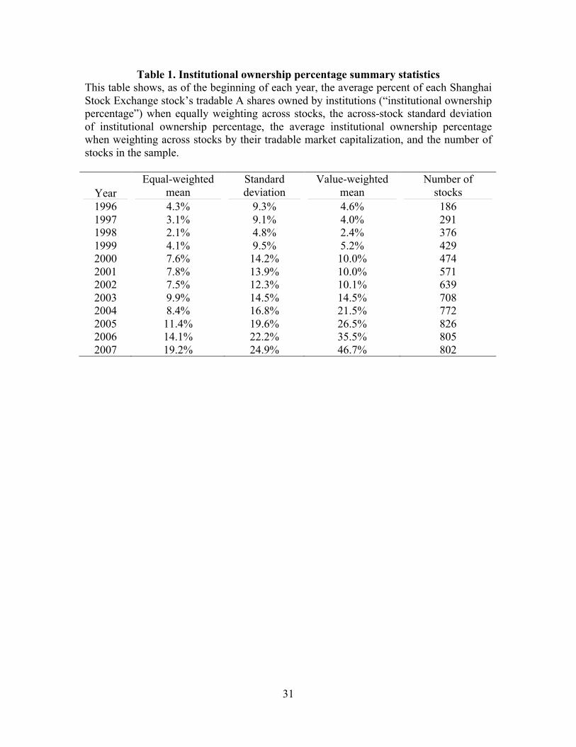
31
Table 1. Institutional ownership percentage summary statistics This table shows, as of the beginning of each year, the average percent of each Shanghai Stock Exchange stock’s tradable A shares owned by institutions (“institutional ownership percentage”) when equally weighting across stocks, the across-stock standard deviation of institutional ownership percentage, the average institutional ownership percentage when weighting across stocks by their tradable market capitalization, and the number of stocks in the sample.
Year Equal-weighted
mean Standard deviation
Value-weighted mean
Number of stocks
1996 4.3% 9.3% 4.6% 186 1997 3.1% 9.1% 4.0% 291 1998 2.1% 4.8% 2.4% 376 1999 4.1% 9.5% 5.2% 429 2000 7.6% 14.2% 10.0% 474 2001 7.8% 13.9% 10.0% 571 2002 7.5% 12.3% 10.1% 639 2003 9.9% 14.5% 14.5% 708 2004 8.4% 16.8% 21.5% 772 2005 11.4% 19.6% 26.5% 826 2006 14.1% 22.2% 35.5% 805 2007 19.2% 24.9% 46.7% 802
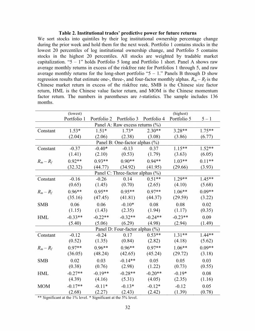
32
Table 2. Institutional trades’ predictive power for future returns We sort stocks into quintiles by their log institutional ownership percentage change during the prior week and hold them for the next week. Portfolio 1 contains stocks in the lowest 20 percentiles of log institutional ownership change, and Portfolio 5 contains stocks in the highest 20 percentiles. All stocks are weighted by tradable market capitalization. “5 – 1” holds Portfolio 5 long and Portfolio 1 short. Panel A shows raw average monthly returns in excess of the riskfree rate for Portfolios 1 through 5, and raw average monthly returns for the long-short portfolio “5 – 1.” Panels B through D show regression results that estimate one-, three-, and four-factor monthly alphas. Rm – Rf is the Chinese market return in excess of the riskfree rate, SMB is the Chinese size factor return, HML is the Chinese value factor return, and MOM is the Chinese momentum factor return. The numbers in parentheses are t-statistics. The sample includes 136 months.
(lowest)
Portfolio 1 Portfolio 2 Portfolio 3 Portfolio 4 (highest)
Portfolio 5 5 – 1 Panel A: Raw excess returns (%)
Constant 1.53* 1.51* 1.73* 2.30** 3.28** 1.75** (2.04) (2.06) (2.38) (3.08) (3.86) (6.77)
Panel B: One-factor alphas (%) Constant -0.37 -0.40* -0.13 0.37 1.15** 1.52** (1.41) (2.10) (0.53) (1.79) (3.63) (6.05) Rm – Rf 0.92** 0.93** 0.90** 0.94** 1.03** 0.11** (32.32) (44.77) (34.92) (41.95) (29.66) (3.93)
Panel C: Three-factor alphas (%) Constant -0.16 -0.26 0.14 0.51** 1.29** 1.45** (0.65) (1.45) (0.70) (2.65) (4.10) (5.68) Rm – Rf 0.96** 0.95** 0.95** 0.97** 1.06** 0.09** (35.16) (47.45) (41.81) (44.37) (29.59) (3.22) SMB 0.06 0.06 -0.10* 0.08 0.08 0.02 (1.15) (1.43) (2.35) (1.94) (1.17) (0.35) HML -0.33** -0.22** -0.32** -0.24** -0.23** 0.09 (5.40) (5.06) (6.29) (4.98) (2.94) (1.49)
Panel D: Four-factor alphas (%) Constant -0.12 -0.24 0.17 0.53** 1.31** 1.44** (0.52) (1.35) (0.84) (2.82) (4.18) (5.62) Rm – Rf 0.97** 0.96** 0.96** 0.97** 1.06** 0.09** (36.05) (48.24) (42.65) (45.24) (29.72) (3.18) SMB 0.02 0.03 -0.14** 0.05 0.05 0.03 (0.38) (0.76) (2.98) (1.22) (0.73) (0.55) HML -0.27** -0.19** -0.28** -0.20** -0.19* 0.08 (4.39) (4.16) (5.31) (4.05) (2.35) (1.16) MOM -0.17** -0.11* -0.13* -0.12* -0.12 0.05 (2.68) (2.27) (2.43) (2.42) (1.39) (0.78) ** Significant at the 1% level. * Significant at the 5% level.
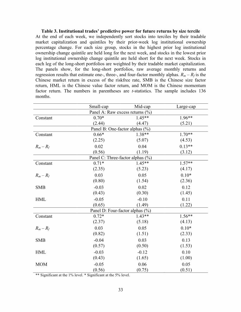
33
Table 3. Institutional trades’ predictive power for future returns by size tercile At the end of each week, we independently sort stocks into terciles by their tradable market capitalization and quintiles by their prior-week log institutional ownership percentage change. For each size group, stocks in the highest prior log institutional ownership change quintile are held long for the next week, and stocks in the lowest prior log institutional ownership change quintile are held short for the next week. Stocks in each leg of the long-short portfolios are weighted by their tradable market capitalization. The panels show, for the long-short portfolios, raw average monthly returns and regression results that estimate one-, three-, and four-factor monthly alphas. Rm – Rf is the Chinese market return in excess of the riskfree rate, SMB is the Chinese size factor return, HML is the Chinese value factor return, and MOM is the Chinese momentum factor return. The numbers in parentheses are t-statistics. The sample includes 136 months. Small-cap Mid-cap Large-cap
Panel A: Raw excess returns (%) Constant 0.70* 1.45** 1.96** (2.44) (4.47) (5.21)
Panel B: One-factor alphas (%) Constant 0.66* 1.38** 1.70** (2.25) (5.07) (4.53) Rm – Rf 0.02 0.04 0.13** (0.56) (1.19) (3.12)
Panel C: Three-factor alphas (%) Constant 0.71* 1.45** 1.57** (2.35) (5.23) (4.17) Rm – Rf 0.03 0.05 0.10* (0.80) (1.54) (2.36) SMB -0.03 0.02 0.12 (0.43) (0.30) (1.45) HML -0.05 -0.10 0.11 (0.65) (1.49) (1.22)
Panel D: Four-factor alphas (%) Constant 0.72* 1.43** 1.56** (2.37) (5.18) (4.13) Rm – Rf 0.03 0.05 0.10* (0.82) (1.51) (2.33) SMB -0.04 0.03 0.13 (0.57) (0.50) (1.53) HML -0.03 -0.12 0.10 (0.43) (1.65) (1.00) MOM -0.05 0.06 0.05 (0.56) (0.75) (0.51) ** Significant at the 1% level. * Significant at the 5% level.
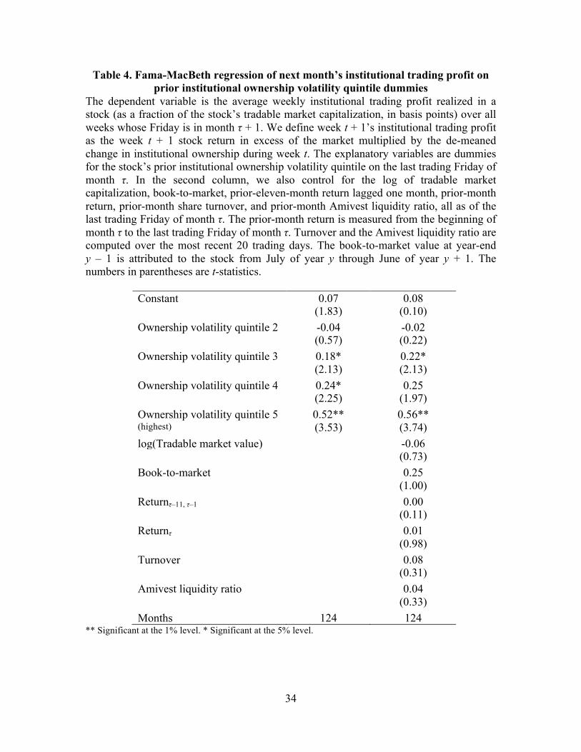
34
Table 4. Fama-MacBeth regression of next month’s institutional trading profit on prior institutional ownership volatility quintile dummies
The dependent variable is the average weekly institutional trading profit realized in a stock (as a fraction of the stock’s tradable market capitalization, in basis points) over all weeks whose Friday is in month τ + 1. We define week t + 1’s institutional trading profit as the week t + 1 stock return in excess of the market multiplied by the de-meaned change in institutional ownership during week t. The explanatory variables are dummies for the stock’s prior institutional ownership volatility quintile on the last trading Friday of month τ. In the second column, we also control for the log of tradable market capitalization, book-to-market, prior-eleven-month return lagged one month, prior-month return, prior-month share turnover, and prior-month Amivest liquidity ratio, all as of the last trading Friday of month τ. The prior-month return is measured from the beginning of month τ to the last trading Friday of month τ. Turnover and the Amivest liquidity ratio are computed over the most recent 20 trading days. The book-to-market value at year-end y – 1 is attributed to the stock from July of year y through June of year y + 1. The numbers in parentheses are t-statistics.
Constant 0.07 0.08 (1.83) (0.10) Ownership volatility quintile 2 -0.04 -0.02 (0.57) (0.22) Ownership volatility quintile 3 0.18* 0.22* (2.13) (2.13) Ownership volatility quintile 4 0.24* 0.25 (2.25) (1.97) Ownership volatility quintile 5 0.52** 0.56** (highest) (3.53) (3.74) log(Tradable market value) -0.06 (0.73) Book-to-market 0.25 (1.00) Returnτ–11, τ–1 0.00 (0.11) Returnτ 0.01 (0.98) Turnover 0.08 (0.31) Amivest liquidity ratio 0.04 (0.33) Months 124 124
** Significant at the 1% level. * Significant at the 5% level.
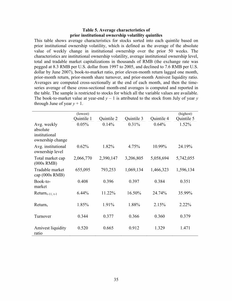
35
Table 5. Average characteristics of prior institutional ownership volatility quintiles
This table shows average characteristics for stocks sorted into each quintile based on prior institutional ownership volatility, which is defined as the average of the absolute value of weekly change in institutional ownership over the prior 50 weeks. The characteristics are institutional ownership volatility, average institutional ownership level, total and tradable market capitalizations in thousands of RMB (the exchange rate was pegged at 8.3 RMB per U.S. dollar from 1997 to 2005, and declined to 7.6 RMB per U.S. dollar by June 2007), book-to-market ratio, prior eleven-month return lagged one month, prior-month return, prior-month share turnover, and prior-month Amivest liquidity ratio. Averages are computed cross-sectionally at the end of each month, and then the time-series average of these cross-sectional month-end averages is computed and reported in the table. The sample is restricted to stocks for which all the variable values are available. The book-to-market value at year-end y – 1 is attributed to the stock from July of year y through June of year y + 1. (lowest)
Quintile 1 Quintile 2 Quintile 3 Quintile 4 (highest)
Quintile 5 Avg. weekly absolute institutional ownership change
0.05% 0.14% 0.31% 0.64% 1.52%
Avg. institutional ownership level
0.62% 1.82% 4.75% 10.99% 24.19%
Total market cap 2,066,770 2,390,147 3,206,805 5,058,694 5,742,055 (000s RMB) Tradable market 655,095 793,253 1,069,134 1,466,323 1,596,134 cap (000s RMB) Book-to- 0.408 0.396 0.397 0.384 0.351 market Returnτ-11, τ-1 6.44% 11.22% 16.50% 24.74% 35.99% Returnτ 1.85% 1.91% 1.88% 2.15% 2.22% Turnover 0.344 0.377 0.366 0.360 0.379 Amivest liquidity 0.520 0.665 0.912 1.329 1.471 ratio
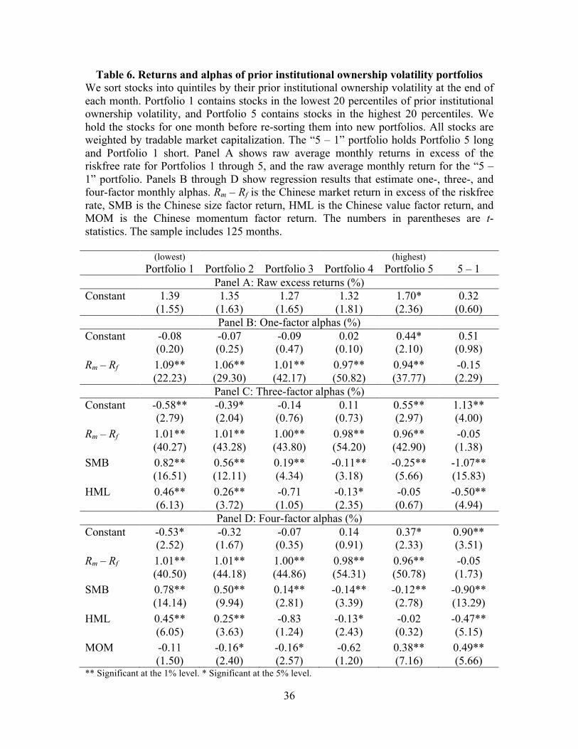
36
Table 6. Returns and alphas of prior institutional ownership volatility portfolios We sort stocks into quintiles by their prior institutional ownership volatility at the end of each month. Portfolio 1 contains stocks in the lowest 20 percentiles of prior institutional ownership volatility, and Portfolio 5 contains stocks in the highest 20 percentiles. We hold the stocks for one month before re-sorting them into new portfolios. All stocks are weighted by tradable market capitalization. The “5 – 1” portfolio holds Portfolio 5 long and Portfolio 1 short. Panel A shows raw average monthly returns in excess of the riskfree rate for Portfolios 1 through 5, and the raw average monthly return for the “5 – 1” portfolio. Panels B through D show regression results that estimate one-, three-, and four-factor monthly alphas. Rm – Rf is the Chinese market return in excess of the riskfree rate, SMB is the Chinese size factor return, HML is the Chinese value factor return, and MOM is the Chinese momentum factor return. The numbers in parentheses are t-statistics. The sample includes 125 months.
(lowest)
Portfolio 1 Portfolio 2 Portfolio 3 Portfolio 4 (highest)
Portfolio 5 5 – 1 Panel A: Raw excess returns (%)
Constant 1.39 1.35 1.27 1.32 1.70* 0.32 (1.55) (1.63) (1.65) (1.81) (2.36) (0.60)
Panel B: One-factor alphas (%) Constant -0.08 -0.07 -0.09 0.02 0.44* 0.51 (0.20) (0.25) (0.47) (0.10) (2.10) (0.98) Rm – Rf 1.09** 1.06** 1.01** 0.97** 0.94** -0.15 (22.23) (29.30) (42.17) (50.82) (37.77) (2.29)
Panel C: Three-factor alphas (%) Constant -0.58** -0.39* -0.14 0.11 0.55** 1.13** (2.79) (2.04) (0.76) (0.73) (2.97) (4.00) Rm – Rf 1.01** 1.01** 1.00** 0.98** 0.96** -0.05 (40.27) (43.28) (43.80) (54.20) (42.90) (1.38) SMB 0.82** 0.56** 0.19** -0.11** -0.25** -1.07** (16.51) (12.11) (4.34) (3.18) (5.66) (15.83) HML 0.46** 0.26** -0.71 -0.13* -0.05 -0.50** (6.13) (3.72) (1.05) (2.35) (0.67) (4.94)
Panel D: Four-factor alphas (%) Constant -0.53* -0.32 -0.07 0.14 0.37* 0.90** (2.52) (1.67) (0.35) (0.91) (2.33) (3.51) Rm – Rf 1.01** 1.01** 1.00** 0.98** 0.96** -0.05 (40.50) (44.18) (44.86) (54.31) (50.78) (1.73) SMB 0.78** 0.50** 0.14** -0.14** -0.12** -0.90** (14.14) (9.94) (2.81) (3.39) (2.78) (13.29) HML 0.45** 0.25** -0.83 -0.13* -0.02 -0.47** (6.05) (3.63) (1.24) (2.43) (0.32) (5.15) MOM -0.11 -0.16* -0.16* -0.62 0.38** 0.49** (1.50) (2.40) (2.57) (1.20) (7.16) (5.66) ** Significant at the 1% level. * Significant at the 5% level.
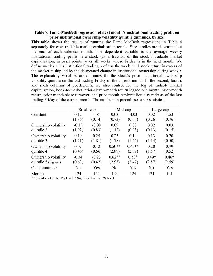
37
Table 7. Fama-MacBeth regression of next month’s institutional trading profit on
prior institutional ownership volatility quintile dummies, by size This table shows the results of running the Fama-MacBeth regressions in Table 4 separately for each tradable market capitalization tercile. Size terciles are determined at the end of each calendar month. The dependent variable is the average weekly institutional trading profit in a stock (as a fraction of the stock’s tradable market capitalization, in basis points) over all weeks whose Friday is in the next month. We define week t + 1’s institutional trading profit as the week t + 1 stock return in excess of the market multiplied by the de-meaned change in institutional ownership during week t. The explanatory variables are dummies for the stock’s prior institutional ownership volatility quintile on the last trading Friday of the current month. In the second, fourth, and sixth columns of coefficients, we also control for the log of tradable market capitalization, book-to-market, prior-eleven-month return lagged one month, prior-month return, prior-month share turnover, and prior-month Amivest liquidity ratio as of the last trading Friday of the current month. The numbers in parentheses are t-statistics. Small-cap Mid-cap Large-cap Constant 0.12 -0.81 0.03 -4.03 0.02 4.53 (1.86) (0.14) (0.73) (0.66) (0.26) (0.76) Ownership volatility -0.15 -0.08 0.09 0.00 0.02 0.03 quintile 2 (1.92) (0.83) (1.12) (0.03) (0.13) (0.15) Ownership volatility 0.19 0.25 0.25 0.19 0.13 0.70 quintile 3 (1.71) (1.81) (1.78) (1.44) (1.14) (0.50) Ownership volatility 0.07 0.12 0.50** 0.45** 0.20 0.79 quintile 4 (0.46) (0.66) (2.89) (2.67) (1.57) (0.52) Ownership volatility -0.34 -0.23 0.62** 0.53* 0.49* 0.46* quintile 5 (highest) (0.63) (0.42) (2.93) (2.47) (2.57) (2.59) Other controls? No Yes No Yes No Yes Months 124 124 124 124 121 121 ** Significant at the 1% level. * Significant at the 5% level.
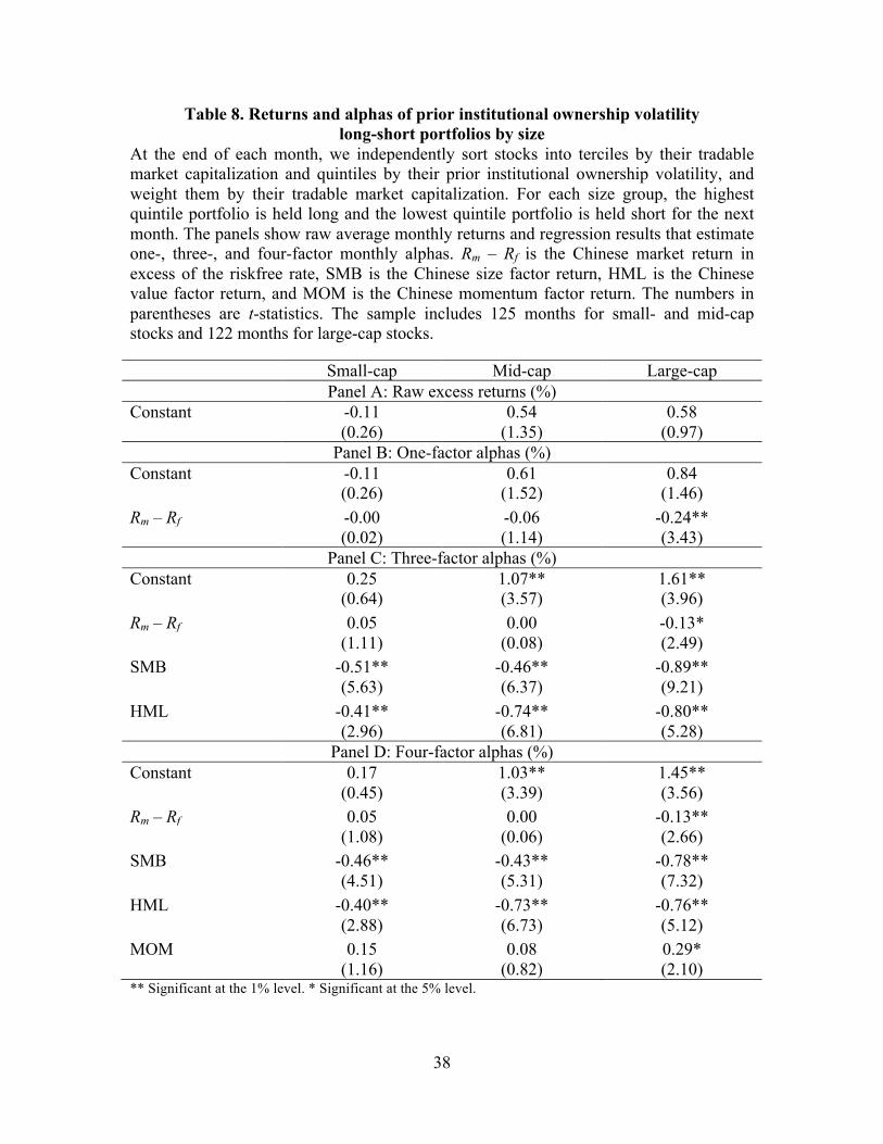
38
Table 8. Returns and alphas of prior institutional ownership volatility long-short portfolios by size
At the end of each month, we independently sort stocks into terciles by their tradable market capitalization and quintiles by their prior institutional ownership volatility, and weight them by their tradable market capitalization. For each size group, the highest quintile portfolio is held long and the lowest quintile portfolio is held short for the next month. The panels show raw average monthly returns and regression results that estimate one-, three-, and four-factor monthly alphas. Rm – Rf is the Chinese market return in excess of the riskfree rate, SMB is the Chinese size factor return, HML is the Chinese value factor return, and MOM is the Chinese momentum factor return. The numbers in parentheses are t-statistics. The sample includes 125 months for small- and mid-cap stocks and 122 months for large-cap stocks. Small-cap Mid-cap Large-cap
Panel A: Raw excess returns (%) Constant -0.11 0.54 0.58 (0.26) (1.35) (0.97)
Panel B: One-factor alphas (%) Constant -0.11 0.61 0.84 (0.26) (1.52) (1.46) Rm – Rf -0.00 -0.06 -0.24** (0.02) (1.14) (3.43)
Panel C: Three-factor alphas (%) Constant 0.25 1.07** 1.61** (0.64) (3.57) (3.96) Rm – Rf 0.05 0.00 -0.13* (1.11) (0.08) (2.49) SMB -0.51** -0.46** -0.89** (5.63) (6.37) (9.21) HML -0.41** -0.74** -0.80** (2.96) (6.81) (5.28)
Panel D: Four-factor alphas (%) Constant 0.17 1.03** 1.45** (0.45) (3.39) (3.56) Rm – Rf 0.05 0.00 -0.13** (1.08) (0.06) (2.66) SMB -0.46** -0.43** -0.78** (4.51) (5.31) (7.32) HML -0.40** -0.73** -0.76** (2.88) (6.73) (5.12) MOM 0.15 0.08 0.29* (1.16) (0.82) (2.10) ** Significant at the 1% level. * Significant at the 5% level.
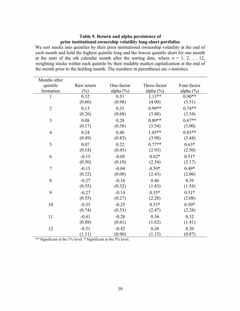
39
Table 9. Return and alpha persistence of
prior institutional ownership volatility long-short portfolios We sort stocks into quintiles by their prior institutional ownership volatility at the end of each month and hold the highest quintile long and the lowest quintile short for one month at the start of the nth calendar month after the sorting date, where n = 1, 2, … 12, weighting stocks within each quintile by their tradable market capitalization at the end of the month prior to the holding month. The numbers in parentheses are t-statistics.
Months after quintile
formation Raw return
(%) One-factor alpha (%)
Three-factor alpha (%)
Four-factor alpha (%)
1 0.32 0.51 1.13** 0.90** (0.60) (0.98) (4.00) (3.51) 2 0.13 0.35 0.99** 0.74** (0.26) (0.68) (3.88) (3.34) 3 0.08 0.28 0.89** 0.67** (0.17) (0.58) (3.54) (3.00) 4 0.24 0.40 1.03** 0.83** (0.49) (0.82) (3.98) (3.44) 5 0.07 0.22 0.77** 0.63* (0.14) (0.45) (2.93) (2.50) 6 -0.15 -0.05 0.62* 0.51* (0.30) (0.10) (2.54) (2.17) 7 -0.15 -0.04 0.59* 0.49* (0.32) (0.08) (2.43) (2.06) 8 -0.27 -0.16 0.46 0.39 (0.55) (0.32) (1.83) (1.54) 9 -0.27 -0.14 0.55* 0.51* (0.55) (0.27) (2.28) (2.08)
10 -0.35 -0.25 0.53* 0.50* (0.74) (0.53) (2.47) (2.28)
11 -0.41 -0.28 0.36 0.32 (0.88) (0.61) (1.62) (1.41)
12 -0.51 -0.42 0.26 0.20 (1.11) (0.90) (1.15) (0.87)
** Significant at the 1% level. * Significant at the 5% level.
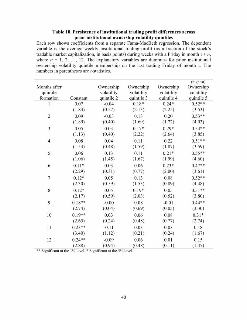
40
Table 10. Persistence of institutional trading profit differences across prior institutional ownership volatility quintiles
Each row shows coefficients from a separate Fama-MacBeth regression. The dependent variable is the average weekly institutional trading profit (as a fraction of the stock’s tradable market capitalization, in basis points) during weeks with a Friday in month τ + n, where n = 1, 2, …, 12. The explanatory variables are dummies for prior institutional ownership volatility quintile membership on the last trading Friday of month τ. The numbers in parentheses are t-statistics.
Months after quintile
formation Constant
Ownership volatility quintile 2
Ownership volatility quintile 3
Ownership volatility quintile 4
(highest) Ownership volatility quintile 5
1 0.07 -0.04 0.18* 0.24* 0.52** (1.83) (0.57) (2.13) (2.25) (3.53) 2 0.09 -0.03 0.13 0.20 0.53** (1.89) (0.40) (1.69) (1.72) (4.03) 3 0.05 0.03 0.17* 0.29* 0.54** (1.13) (0.40) (2.22) (2.64) (3.85) 4 0.08 0.04 0.11 0.22 0.51** (1.54) (0.48) (1.59) (1.87) (3.59) 5 0.06 0.13 0.11 0.21* 0.55** (1.06) (1.45) (1.67) (1.99) (4.60) 6 0.11* 0.03 0.06 0.23* 0.47** (2.29) (0.31) (0.77) (2.00) (3.61) 7 0.12* 0.05 0.13 0.08 0.52** (2.30) (0.59) (1.53) (0.89) (4.48) 8 0.12* 0.05 0.19* 0.05 0.51** (2.17) (0.59) (2.03) (0.52) (3.80) 9 0.18** -0.00 0.08 -0.01 0.44**
(2.74) (0.04) (0.69) (0.05) (3.30) 10 0.19** 0.03 0.06 0.08 0.31* (2.65) (0.24) (0.48) (0.77) (2.74)
11 0.23** -0.11 0.03 0.03 0.18 (3.40) (1.12) (0.21) (0.24) (1.67)
12 0.24** -0.09 0.06 0.01 0.15 (2.88) (0.94) (0.48) (0.11) (1.47)
** Significant at the 1% level. * Significant at the 5% level.

41
Table 11. Institutional ownership change next month by prior institutional ownership volatility quintile
This table shows Fama-MacBeth regression coefficients. The dependent variable is next month’s change in a stock’s institutional ownership percentage. (Its unit is percentage points, so that a value of 1 corresponds to 1%.) The explanatory variables are dummies for the prior institutional ownership volatility quintile the stock belongs to on the last trading Friday of the current month. The numbers in parentheses are t-statistics.
Constant 0.23** (7.76) Ownership volatility quintile 2 0.04 (1.45) Ownership volatility quintile 3 0.02 (0.44) Ownership volatility quintile 4 0.00 (0.05) Ownership volatility quintile 5 -0.53** (highest) (5.20) Months in sample 124
** Significant at the 1% level. * Significant at the 5% level.
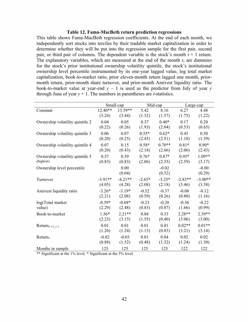
42
Table 12. Fama-MacBeth return prediction regressions This table shows Fama-MacBeth regression coefficients. At the end of each month, we independently sort stocks into terciles by their tradable market capitalization in order to determine whether they will be put into the regression sample for the first pair, second pair, or third pair of columns. The dependent variable is the stock’s month τ + 1 return. The explanatory variables, which are measured at the end of the month τ, are dummies for the stock’s prior institutional ownership volatility quintile, the stock’s institutional ownership level percentile instrumented by its one-year lagged value, log total market capitalization, book-to-market ratio, prior eleven-month return lagged one month, prior-month return, prior-month share turnover, and prior-month Amivest liquidity ratio. The book-to-market value at year-end y – 1 is used as the predictor from July of year y through June of year y + 1. The numbers in parentheses are t-statistics. Small-cap Mid-cap Large-cap Constant 12.40** 13.59** 5.42 8.16 6.27 4.48 (3.24) (3.44) (1.32) (1.57) (1.75) (1.22) Ownership volatility quintile 2 0.04 0.05 0.37 0.40* 0.17 0.20 (0.22) (0.26) (1.93) (2.04) (0.53) (0.65) Ownership volatility quintile 3 0.06 0.07 0.55* 0.62* 0.45 0.50 (0.20) (0.25) (2.45) (2.51) (1.18) (1.39) Ownership volatility quintile 4 0.07 0.15 0.58* 0.70** 0.81* 0.90* (0.20) (0.43) (2.18) (2.66) (2.06) (2.43) Ownership volatility quintile 5 0.37 0.39 0.76* 0.87* 0.95* 1.09** (highest) (0.83) (0.83) (2.06) (2.35) (2.59) (3.17) Ownership level percentile 0.00 -0.02 -0.00 (0.04) (0.52) (0.29) Turnover -3.91** -4.21** -2.65* -3.25* -2.83** -3.00** (4.05) (4.28) (2.08) (2.18) (3.46) (3.58) Amivest liquidity ratio -3.26* -3.19* -0.52 -0.37 -0.08 -0.12 (2.21) (2.08) (0.59) (0.26) (0.80) (1.16) log(Total market -0.59* -0.68* -0.23 -0.28 -0.36 -0.22 value) (2.29) (2.48) (0.83) (0.87) (1.66) (0.99) Book-to-market 1.56* 2.21** 0.88 0.33 2.28** 2.39** (2.23) (3.15) (1.55) (0.40) (3.06) (3.00) Returnτ–11, τ–1 0.01 0.01 0.01 0.01 0.02** 0.01** (1.26) (1.24) (1.13) (0.83) (3.21) (3.14) Returnτ -0.02 -0.03 0.01 0.04 0.02 0.02 (0.88) (1.52) (0.48) (1.32) (1.24) (1.30) Months in sample 125 125 125 125 122 122 ** Significant at the 1% level. * Significant at the 5% level.
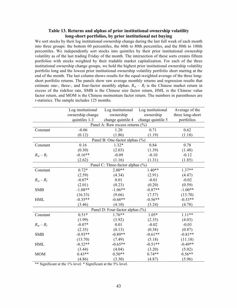
43
Table 13. Returns and alphas of prior institutional ownership volatility long-short portfolios, by prior institutional net buying
We sort stocks by their log institutional ownership change during the last full week of each month into three groups: the bottom 60 percentiles, the 60th to 80th percentiles, and the 80th to 100th percentiles. We independently sort stocks into quintiles by their prior institutional ownership volatility as of the last trading Friday of the month. The intersection of these sorts creates fifteen portfolios with stocks weighted by their tradable market capitalization. For each of the three institutional ownership change groups, we hold the highest prior institutional ownership volatility portfolio long and the lowest prior institutional ownership volatility portfolio short starting at the end of the month. The last column shows results for the equal-weighted average of the three long-short portfolio returns. The panels show raw average monthly returns and regression results that estimate one-, three-, and four-factor monthly alphas. Rm – Rf is the Chinese market return in excess of the riskfree rate, SMB is the Chinese size factor return, HML is the Chinese value factor return, and MOM is the Chinese momentum factor return. The numbers in parentheses are t-statistics. The sample includes 125 months. Log institutional
ownership change quintiles 1-3
Log institutional ownership
change quintile 4
Log institutional ownership
change quintile 5
Average of the three long-short
portfolios Panel A: Raw excess returns (%)
Constant -0.06 1.20 0.71 0.62 (0.12) (1.86) (1.19) (1.18)
Panel B: One-factor alphas (%) Constant 0.16 1.32* 0.84 0.78 (0.30) (2.03) (1.39) (1.48) Rm – Rf -0.16** -0.09 -0.10 -0.12 (2.62) (1.16) (1.31) (1.85)
Panel C: Three-factor alphas (%) Constant 0.72* 2.00** 1.40** 1.37** (2.59) (4.34) (2.91) (4.47) Rm – Rf -0.07* 0.01 -0.01 -0.02 (2.01) (0.23) (0.20) (0.59) SMB -1.08** -1.06** -0.87** -1.00** (16.33) (9.66) (7.57) (13.70) HML -0.35** -0.68** -0.56** -0.53** (3.46) (4.10) (3.24) (4.78)
Panel D: Four-factor alphas (%) Constant 0.51* 1.76** 1.05* 1.11** (1.99) (3.92) (2.35) (4.03) Rm – Rf -0.07* 0.01 -0.02 -0.03 (2.35) (0.13) (0.38) (0.87) SMB -0.93** -0.89** -0.61** -0.81** (13.70) (7.49) (5.18) (11.18) HML -0.32** -0.65** -0.51** -0.49** (3.44) (4.04) (3.20) (5.02) MOM 0.43** 0.50** 0.74** 0.56** (4.86) (3.30) (4.87) (5.96) ** Significant at the 1% level. * Significant at the 5% level.
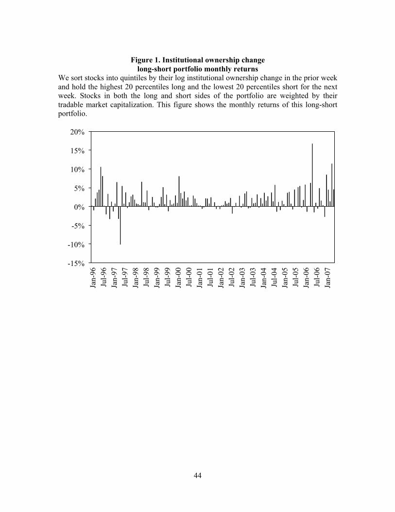
44
Figure 1. Institutional ownership change
long-short portfolio monthly returns We sort stocks into quintiles by their log institutional ownership change in the prior week and hold the highest 20 percentiles long and the lowest 20 percentiles short for the next week. Stocks in both the long and short sides of the portfolio are weighted by their tradable market capitalization. This figure shows the monthly returns of this long-short portfolio.
-15%
-10%
-5%
0%
5%
10%
15%
20%
Jan-
96
Jul-9
6 Ja
n-97
Ju
l-97
Jan-
98
Jul-9
8 Ja
n-99
Ju
l-99
Jan-
00
Jul-0
0 Ja
n-01
Ju
l-01
Jan-
02
Jul-0
2 Ja
n-03
Ju
l-03
Jan-
04
Jul-0
4 Ja
n-05
Ju
l-05
Jan-
06
Jul-0
6 Ja
n-07
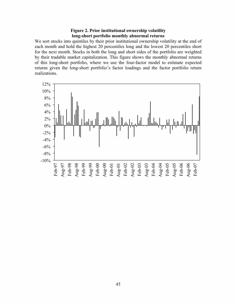
45
Figure 2. Prior institutional ownership volatility long-short portfolio monthly abnormal returns
We sort stocks into quintiles by their prior institutional ownership volatility at the end of each month and hold the highest 20 percentiles long and the lowest 20 percentiles short for the next month. Stocks in both the long and short sides of the portfolio are weighted by their tradable market capitalization. This figure shows the monthly abnormal returns of this long-short portfolio, where we use the four-factor model to estimate expected returns given the long-short portfolio’s factor loadings and the factor portfolio return realizations.
-10% -8% -6% -4% -2% 0% 2% 4% 6% 8%
10% 12%
Feb-
97
Aug
-97
Feb-
98
Aug
-98
Feb-
99
Aug
-99
Feb-
00
Aug
-00
Feb-
01
Aug
-01
Feb-
02
Aug
-02
Feb-
03
Aug
-03
Feb-
04
Aug
-04
Feb-
05
Aug
-05
Feb-
06
Aug
-06
Feb-
07