Information Asymmetries in the Mortgage BackedSecurities Market
Chris Downing, Dwight Jaffee and Nancy Wallace∗
May 3, 2005
∗Please address correspondence to (Downing): Jones Graduate School of Management, Rice University,6100 Main Street, Room 249 - Mail Stop 531, Houston, TX 77005. Phone: (713) 348-6234. Fax: (713) 348-6296. E-Mail: [email protected]. (Jaffee): Haas School of Business, University of California at Berkeley,Berkeley, CA 94720. Phone: (510) 642-1273. Fax: (510) 643-7357. E-Mail: [email protected].(Wallace): Haas School of Business, University of California at Berkeley, Berkeley, CA 94720. Phone: (510)642-4732. Fax: (510) 643-7357. E-Mail: [email protected].
1

Abstract
One of the primary results of studying asymmetric information as part of informa-tion economics over the last 30 years has been a theory of markets for lemons—thatis, markets for goods that are likely to be of poor quality. Unfortunately, it has provendifficult to directly test the lemons theory because the causative factor—asymmetricinformation—implies that key quality variables are not observable. In this paper, weavoid this problem by studying the market for mortgage backed securities (MBS), amarket which exhibits significant asymmetric information on an ex ante basis, but expost reveals individual security qualities. In this market, some of the MBS producedin any given month are repackaged into multi-class security structures where certainclasses enjoy higher priority claims on the underlying mortgage cash flows than others.As shown in DeMarzo and Duffie (1998), these security structures are optimal whenthe market values of the underlying assets are sensitive to private information heldby the issuer of the securities. Utilizing a comprehensive dataset of all Freddie MacGold Participation Certificates (PCs) issued between 1991 and 2002, we show that,consistent with lemons theory, the PCs used to construct multi-class MBS tend tobe of lower quality than other PCs. Our results suggest that structured multi-classsecurities, which after years of explosive growth now surpass traditional single-classsecurities in importance, are a market response to the problem of efficiently allocatingcapital when problems of asymmetric information are acute. Our results also haveimplications for public policies related to government sponsored enterprises.
2
1 Introduction
One benefit of studying asymmetric information as part of information economics over the
last 35 years has been a theory of markets for lemons—that is, for goods likely to be of
poor quality. The seminal paper by Akerloff (1970) shows how in markets with asymmetric
information, only goods of the lowest quality (“lemons”) are traded. Unfortunately, it has
proven difficult to test the theory of markets for lemons because the causative factor—
asymmetric information—necessarily makes it difficult to observe the key quality variables
that determine goods prices.1
In this paper, we use the market for mortgage-backed securities (MBS) to test the theory
of lemons markets. Mortgage-backed securities are bonds secured by pools of residential
home mortgages, with the mortgage payments passed through to the holders of the MBS.
One of the largest bond markets in the U.S., the MBS market is interesting in its own right.2
In the context of testing lemons theory, however, the MBS market is of interest for two
reasons. First, the market exhibits significant information asymmetries among various of
its participants. Mortgage-backed securities primarily trade in broker markets with little
systematic public disclosure of either transaction prices or trade volumes.3 Moreover, the
market is dominated by two government sponsored enterprises (GSEs), Fannie Mae and
Freddie Mac. These GSEs have chosen not to release all of the information available to them
regarding the mortgages backing MBS.4 The market thus contains an important degree of
asymmetric information ex ante concerning the prices and likely payment behavior of the
mortgages in different MBS pools. However, the payment behavior of each mortgage pool
is revealed ex post in terms of the rate of terminations (sum of prepayments and defaults).
Termination rates are critical determinants of the ex post returns on MBS because discounted
MBS (those with coupons below the current par coupon) will earn excess returns relative to
other MBS if their termination rates turn out to be faster than the rates embedded in the
initial market prices, and vice versa for premium MBS.
1The only other direct test of the lemons model that we are aware of is Bond (1982).2In 2004, originations of home mortgages in the United States totaled $2.8 trillion, of which $1.8 trillion,
or 65%, were repackaged as MBS (Inside MBS & ABS, February 18, 2005).3This stands in contrast to many other securities markets; most recently, the other major bond markets
have increased the transparency of their operations. In the municipal bond market, the Municipal SecuritiesRulemaking Board has implemented a trade reporting and dissemination system and plans to graduallymove that market to real-time reporting of transaction prices and volumes. In the corporate bond market,including the high-yield submarket, the National Association of Securities Dealers has implemented a systemmuch like that in the muni market.
4The issue of asymmetric information in the MBS market is studied in United States Department of theTreasury (2003), a staff report of the Task Force on Mortgage-Backed Securities Disclosure. Following therelease of this report, both GSEs “voluntarily” expanded the range of information they release on newlyissued MBS, although potentially important information is still not released.
3

The second reason that the MBS market is of interest is that a substantial share of MBS
are repackaged into multi-class securities by the GSEs and investment banks. In a multi-
class securitization, some fraction of the total face value of the securities is allocated to
senior bond classes with first priority claims on the cash flows of the underlying assets, while
the more junior classes are impacted by low quality collateral. The prices of the securities
remain efficient, since asymmetric information has little relevance to the senior classes, while
the junior classes are traded among informed agents.5 As shown by DeMarzo (2003) and
DeMarzo and Duffie (1998), these capital structures are optimal when the values of the
underlying assets are sensitive to private information held by the security issuer.6 Hence
multi-class MBS can be viewed as a market response to the lemons problem that might
otherwise render inoperative the market for single-class MBS.
We base our empirical work on a comprehensive dataset of all Freddie Mac Gold Partic-
ipation Certificates (PCs) issued between 1991 and 2002. We compare the performance of
PCs used to create single-class securities versus those used to create structured multi-class
securities. Our key result is that, in rising interest-rate environments, pools selected as col-
lateral for multi-class securitizations tend to return principal at a significantly slower rate
than pools that are not so selected, even after controlling for all of the publicly-available
information about these pools. Similarly, in falling interest-rate environments, pools that
are selected as collateral for multi-class securitizations return principal at a faster rate than
the pools that are not so selected. Hence in the absence of a price discount to reflect the dif-
ferential payment speeds, MBS pools used as collateral for multi-class securitizations would
earn lower returns than the those pools not used in the multi-class market; in other words,
the multi-class MBS market is a market for lemons. Employing a model of MBS prices,
we estimate that the pools backing multi-class MBS are discounted, on average, by approx-
imately six cents per hundred dollars of principal, with discounts as high as 20 cents per
hundred dollars in certain instances.7
Understanding the effects of information asymmetries in the MBS market is also relevant
5On the other hand, the prices would be inefficient if uninformed agents tend to overbid or underbid forpools, reflecting the limited information available to them. Unfortunately, we are unable to test for pricingefficiency because we know of no continuing source of prices for individual MBS pools. However, our teststo determine which MBS pools are lemons are unaffected by whether the actual market prices are efficientor not.
6A number of other security design papers have focused on the role of asset bundling in markets withinformation asymmetries (see, for example, Diamond and Verrecchia (1991); Boot and Thakor (1997); Glaeserand Kallal (1997)). These papers focus on the information asymmetries between security issuers, investment-bank intermediaries, and final investors. None of these papers contain empirical tests; to our knowledge thispaper is the first to use data on multi-class securities to test the lemons theory.
7Recalling that the total size of the market for structured MBS is several hundred billion dollars, theaggregate discount is substantial.
4

to public policymakers and market participants. Informational asymmetries in this market
are important to policymakers because regulatory oversight dictates many aspects of the
MBS market structure and likely contributes to the dominance of the GSEs in both MBS
trading and portfolio investment. Furthermore, the functioning of the market is of concern
to policymakers who focus on the interests of U.S. homeowners, since about two-thirds of
residential mortgage loans originated in the U.S. are securitized. MBS are also very widely
held investment instruments, hence issues related to the performance of MBS are likely to
have implications for the broader U.S. financial markets, as well.
This paper is organized as follows. In the next section, we discuss the institutional details
and information asymmetries in the market for Freddie Mac PCs. Section 3 lays out our
strategy for identifying PCs that are lemons and presents our empirical results. Section 4
concludes.
2 Information Asymmetries and Freddie Mac PCs
2.1 Market Overview
Most Freddie Mac PCs have been issued through the 30 Year Gold Program. As shown
in Table 1, total monthly pool issuance from 1991 through 2002 was 85,988 pools which in
aggregate accounted for 12.5 million mortgages and $1.5 trillion of mortgage principal. The
recent refinancing boom of 2001 and 2002 coincided with the introduction of 15 year Freddie
Mac PCs, however, for the most part PCs are collateralized with 30-year mortgages. The
Balloon PCs are collateralized by mortgages that amortize over 30 years but are due in full
in five or seven years; Mini PCs are smaller seasoned pools. As can be seen from Table 1,
these latter two types of collateral back only small shares of total PC issuance.
Freddie Mac issues most of its PCs through swap programs in which mortgage originators
accumulate conforming mortgages into pools that are then swapped for Freddie Mac PCs.
The PCs obtained by the originators via swaps are collateralized by the same mortgages that
the originator transfers to Freddie Mac. The pool sizes are surprisingly small, averaging just
172 mortgages in 2002. In Table 2, we provide some summary statistics for the 61,929
unseasoned PC pools in our sample. Unseasoned pools are those with a weighted-average
remaining term of 359 or more months at the time of origination. We focus on these pools in
our empirical analysis because forecasting the seasoning patterns of mortage pools is a key
element in selecting lemons.8 For these pools, the weighted average coupons vary by year
8Seasoning refers to the conventional wisdom that, for a given interest-rate decline, mortgage poolscloser to their origination dates tend to exhibit slower prepayments. In contrast, “burnout” refers to theconventional wisdom that a given decline in interest rates elicits less and less prepayment response from a
5

reflecting the term structure of interest rates at the time of origination; in general, long-term
interest rates are falling over our sample period, as reflected in the declining weighted-average
coupon rates. In our empirical tests, we focus on unseasoned pools with a weighted average
remaining term of 359 months at the origination of the pool. The average balance in these
pools ranges from about $2.6 million to $27.6 million and the trend appears to be toward
larger pool balances in the later years of the sample.
Freddie Mac and Fannie Mae both repurchase large shares of their own guaranteed pools,
as well as pools of the other GSE. As shown in Figure 1, beginning in 1993, Freddie Mac has
steadily increased its holdings of its own PCs. By year-end 2002, Freddie Mac’s portfolio
holdings of it own PCs accounted for $393 billion out of the total outstanding stock of $1.162
trillion. Freddie Mac repurchases its PCs through trades with investment banks in a brokered
market.9
2.2 PC Market Microstructure
Freddie Mac PCs are traded on both a to-be-announced and a pool-specific basis. Unfortu-
nately, there is no publicly available information documenting aggregate trade volumes on
these markets. Moreover, there is little information concerning the trade volumes in indi-
vidual securities, but the information that does exist suggests that individual pools do not
trade frequently.10
In the to-be-announced (TBA) market, pools are traded for forward delivery on a specified
settlement day. Prices quoted in the TBA market are for contracts that specify only the
type of PC (e.g., 30-year fixed rate Freddie Mac Gold PC), the weighted average coupon,
and the date of delivery. Pools to be assembled for future delivery do not have determinate
pool-specific characteristics at the time of forward contracting, so it is not feasible to embed
such pool-specific characteristics into the prices of the forward contracts.
As suggested by Glaeser and Kallal (1997), one possible interpretation of the TBA mar-
ket is that the TBA prices coalesce around the worth of the least valuable, but deliverable,
mortgage pools.11 The market gains liquidity from TBA trading if there is less uncertainty
about the value which the market should assign to the worst security than about the values
which the market should assign to more valuable securities. As shown by Gorton and Pen-
pool as it ages.9These purchases are primarily financed by the issuance of Agency bonds.
10According to the Bond Market Association, in 2004 the daily trading volume for third party trades ofMBS equaled about 4% of the outstanding value, compared to a 6% ratio for U.S. Treasuries.
11Mortgage originators are also active traders of the PCs obtained through the swap market; these PCsare collateralized by their own mortgages. From the viewpoint of the originator the decision to sell a poolTBA must reflect a trade-off between the opportunity cost of not selling versus the cost of selling at a pricebelow fair value price.
6

nachi (1990) the traded security in such a market would be free from idiosyncratic risk and
vulnerable only to systematic risk.
The pool-specific market—the stipulations (STIPs) market—is an important alternative
to trading Freddie Mac PCs. In this market, pool specific information is available on the
identity of the mortgage originator, and, more recently, borrower credit scores, the geographic
composition of the pool, loan-to-value ratios, and pool termination histories.12 In theory,
PC prices should impound all of the known factors that determine the expected cash flows
of the pools. Presumably, traders who could achieve the most accurate predictions of future
cash flows would be at an informational advantage in the STIPs market.
2.3 The REMIC Market
The multi-class MBS, or “REMIC”, market is another important source of demand for PCs.13
As noted earlier, an important benefit of the multi-class structure is that some of the classes
can be assigned higher priority claims on the underlying mortgage cash flows, rendering the
MBS cash flows relatively more predictable even if the underlying pools exhibit termination
rates that fluctuate substantially through time. The single-class PCs that underlie Freddie
Mac’s REMIC securities are contributed by investment banks and Freddie Mac from their
respective inventories. In exchange they obtain pro-rata shares of the REMIC securities.
Freddie Mac also earns a fee for its work in creating the multi-class security, and the invest-
ment banks profit if the aggregate value of the multi-class security exceeds the value of the
single-class PCs from which it was created.14
In Figure 2, we plot the breakdown of unseasoned PC balances backing multi-class
(REMIC) and single-class (non-REMIC) MBS.15 The outstanding share of PC balances that
were held in non-REMICs grew dramatically starting in 1997. As can be seen by compar-
ing figures 1 and 2, the relative decrease in the outstanding proportions of PCs that were
securitized into REMICs is coincident with the rise in Freddie Mac’s purchases of PCs for
its retained portfolio. The share of REMIC to non-REMIC principal converged in late 2002,
largely due to the very rapid payout rates on the non-REMIC collateral.
12Pool-specific informtion on credit scores and the loan-to-value distibutions for the pools were not madeavailable before June of 2003
13The acronym “REMIC” refers to Real Estate Mortgage Investment Conduit, a special legal structureused to issue structured MBS; the term “collateralized mortgage obligation” or “CMO” often refers to thesame legal structure. Henceforth we use the terms REMIC and multi-class MBS interchangeably.
14This requires that the markets be initially incomplete, in the sense that the cash flow patterns offered bythe multi-class security did not previously exist in the market. See Oldfield (2000) for a further discussionof how value is added by the creation of multi-class securities.
15Many PC pools had fractions of their overall principal balance allocated to REMICs and many PC poolswere fractionally allocated to a number of different REMICs. We assigned all of these fractional principalallocations to their respective REMIC and non-REMIC market segments.
7

Table 3 summarizes Freddie Mac’s 2003 mortgage-related holdings. As shown, $472
billion, or 29 percent, of the total issued Freddie Mac PCs have been converted into structured
multi-class REMICs. Freddie Mac held in its own retained portfolio 34 percent of the total
issued single-class PCs and 26 percent of the total issued REMICs. The fact that Freddie
Mac holds REMICs despite its likely superior knowledge of mortgage termination trends is
consistent with the theory of pooling and tranching outlined at the outset (DeMarzo and
Duffie (1998)). Superior termination information in the REMIC market can be used to
more accurately value the subordinate REMIC classes in which most of the termination risk
resides; since Freddie Mac is the better informed agent, it is likely that they hold these
subordinate classes. Unfortunately, we do not have information concerning where in each
REMIC bond structure Freddie Mac concentrates its purchases, so this conjecture cannot
be verified.
As noted above, Freddie Mac and the investment banks receive prorated shares of newly
created REMICs. However, the shares depend on the principal value, and not the market
price, of the single-class PCs they contribute to the pool of PCs backing the REMIC se-
curities. There is thus a strong incentive for each firm to provide only low value PCs as
their contribution to the underlying pools. To be sure, other factors will also enter into
the decision of which PCs to contribute. For example, this procedure provides a convenient
outlet for the investment banks to sweep their inventory of small bits and pieces of PCs into
REMIC pools, which otherwise would have to be sold at a discounted price as odd lots. In
any case, the outcome is that the single-class PCs used to create REMICs are likely to be
lemons relative to the PCs that are not used for this purpose. In the next section, we will
consider the degree to which pools selected to back REMICs are, in fact, lemons.
3 Are Multi-Class MBS Lemons?
An important feature of the Freddie Mac PC market is that the true quality of all PCs
can be known ex post due to the registration requirements and reporting conventions of
the securitized mortgage bond market. Freddie Mac provides publicly available information
on the termination speeds of all Freddie Mac PCs at the end of every month. It also
provides registration reports on the cusips for PC pools that are included in REMICs.16. A
possible concern is that the timing of these reporting practices might allow the GSE’s and
the commercial banks to exploit private information on termination speeds. For example,
this information could be used to identify which pools should be allocated to the REMIC
market rather retained for portfolio investment.
16This usually occurs several months after the origination of the individual PC pools
8

We identify two channels for informed agents to exploit information asymmetries in the
PC market. A tactical selection channel is associated with market timing and exploiting
the short-run persistence of termination speeds. The tactical selection channel enables in-
formed agents to identify and reject lemon pools using pool-specific termination speeds that
are known before other agents in the market.17 The tactical selection channel operates
through short-run timing effects at pool origination. Informed agents exploit early arriving
information on the initial termination experience of PC pools to forecast future cumulative
termination speeds. For this channel to be a viable mechanism, a pool’s early termination
speed must be persistent enough to reliably forecast the later termination speed of the pool.
A strategic selection channel is associated with the commercial banks’ and Freddie Mac’s
modelling expertise in long-run forecasting of termination speeds at the pool-level. This
channel requires informed agents to identify lemons ex ante. Lemon PCs are those expected
to have slow long-run termination speeds in rising interest-rate environments (their weighted
average coupons are below the current mortgage rate) and fast long-run termination speeds
in falling interest-rate environments (the weighted average coupon is above the current mort-
gage rate). Pools such as these would then be allocated to the REMIC market where their
elevated termination risk can be re-engineered into less risky senior bonds (suitable for un-
informed low-yield investors) and risky subordinated bonds (suitable for informed high-yield
investors). Pools that are expected to return principal rapidly in rising interest-rate envi-
ronments, and vice-versa, would be considered non-lemons and would be held directly.
3.1 Reduced-Form Analysis
We test for the existence of the tactical and strategic selection channels by regressing the
cumulative terminations of PC pools on an ex ante measure of initial terminations for the
tactical channel and a contemporaneous measure of cumulative interest-rate changes for
the strategic channel.18 We also include a number of other controls for publicly available
17Recent testimony by Armando Falcon Jr., director of the Office of Federal Housing Enterprise Oversight,suggested that “...Fannie Mae was performing a sorting and sifting process involving actual scoring of tradesthat allowed the enterprise to retain high quality loans for its portfolio while fulfilling matched buy-and-selltrades using lower quality collateral. The enterprise referred to this process internally as “keep the best;sell the rest”.” Inside MBS & ABS April, 8, 2005. The Wall Street Journal (April 7, 2005) also reportedthat the GSE regulator, Mr. Falcon, stated that, “.. Fannie’s policy allowed it to wait until the end ofthe month in which a transaction is settled to decide whether to sell or hold a given security,” which is inviolation of generally accepted accounting principles. A 2003 internal report completed by Baker, Botts LLPalso reported that ”...Freddie’s MBS trading unit routinely identified the best securities for the company’sinvestment arm.” Inside MBS & ABS, April, 8, 2005.
18The mortgages that appear in the pools we focus on are fully amortizing, which means that at the endof their scheduled 30-year terms, the remaining balance on each mortgage is zero, assuming no prepayment,default, or early payments of principal (curtailments). Each month, the mortgage payment is constant,implying that the relative shares of interest and principal in the total payment are changing each month.
9
information, such as the pool’s weighted average origination coupon, the financial institution
that originated the mortgages, time dummies for vintage effects, and the cumulative changes
in the ten-year Treasury rate over the given holding period. We focus on comparisons of
“pure” REMIC pools, where 100 percent of the principal is in REMIC, with pure non-REMIC
pools where none of the principal has been re-securitized.
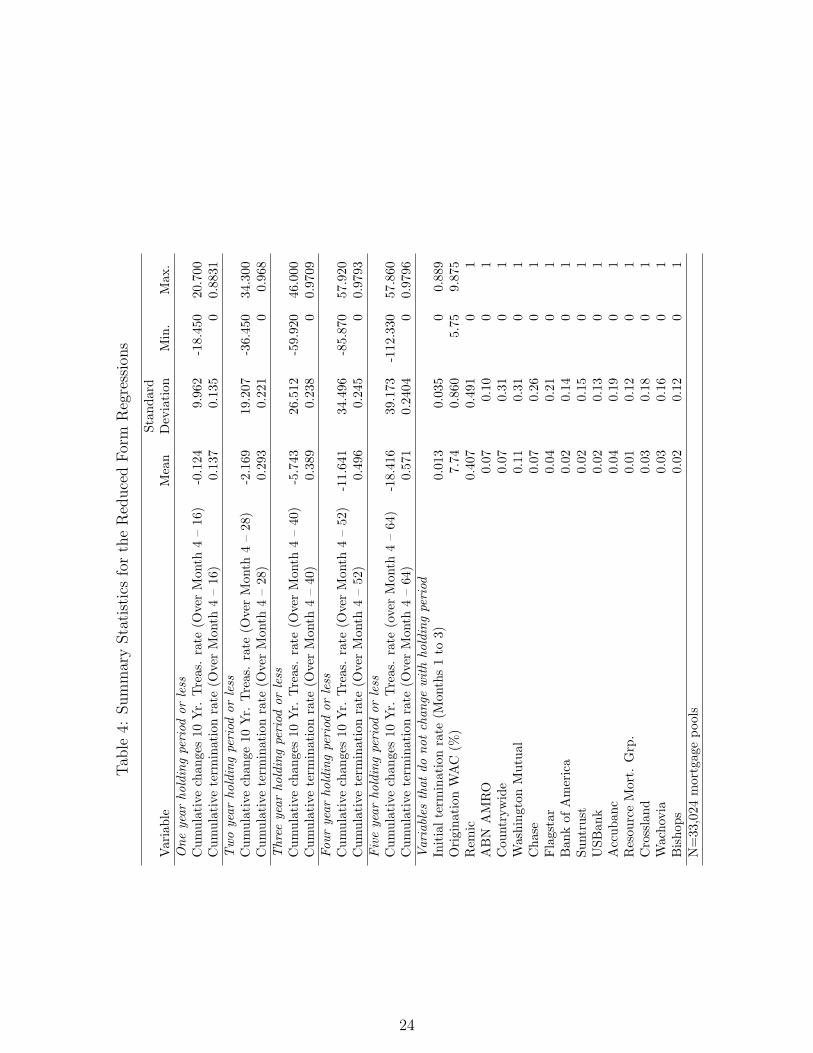
Table 4 provides some summary statistics for the variables that we use in our reduced-
form analysis. The tactical channel is identified as cumulative unscheduled mortgage ter-
minations (prepayments and defaults) over the first three months of a pool.19 The average
three-month cumulative termination rate is 1.3 percent of the original pool balance, with
a range from zero to 89 percent, and the standard deviation is quite large, indicating that
some pools “burn out” very rapidly while others experience very little in the way of termina-
tions over the first three months. The cumulative termination rates over the longer horizons
exhibit a similar high degree of dispersion, and the average cumulative termination rate rises
with the investment horizon, as it is natural to expect given how the variable is constructed.
The cumulative changes in the ten-year Treasury rate from the fourth month to the end
of the holding period are a measure of the pool’s exposure to fluctuating Treasury rates given
both the pool vintage and the investment holding period. As shown in Table 4, the mean
of this variable becomes more negative as the holding period increases, reflecting the fact
that, in general, Treasury rates were falling over the period of study. Like the cumulative
termination rates, the standard deviations are quite large, reflecting the wide variation in
the interest-rate experiences looking across the vintages of the pools.
We include in our sample only “pure” REMIC and non-REMIC pools—that is, pools
that are either entirely or not at all devoted to REMIC re-securitizations. Under this strict
definition, REMIC pools account for about 7 percent of the sample; in our restricted sample,
REMIC pools make up about 40 percent of the pools. However, there is considerable variation
in the share of REMIC pools over the vintages, as suggested by Figure 2. We also report the
market shares of various mortgage originators. The shares are in general low, as there are
many originators in that highly competitive segment of the residential mortgage market.
We report the reduced form regression results in Table 5. We find a positive and statis-
tically significant effect of the cumulative initial termination rates on the subsequent cumu-
lative termination experience for most investment horizons.20 The statistical and economic
19Because Freddie Mac guarantees the Gold PCs against default, default events look like prepayments. Itis important to emphasize that we do not include scheduled interest and principal payments in our measure;thus the dependent variable is thus one less the survival factor for each pool at each time horizon. SeeBartlett (1989) for details on survival factors.
20It is important to note that here we are conditioning only on the first three months of termination historyfor each pool. We have also examined the predictive content of three-month average termination rates forfuture termination rates well after origination. These regressions indicate that, over short horizons, the most
10
importance of the tactical channel, however, appears to diminish over longer investment hori-
zons. For the five year investment horizon, in particular, the short-term tactical advantage
of knowing the early pool experience does not allow a statistically significant forecast for
future termination rates, though sample-truncation may be an issue at this horizon. At the
one-year horizon, the interaction of initial terminations with the REMIC indicator is posi-
tive and statistically significant. The interaction term is slightly negative and insignificant
for the two-year horizon, but is negative and significant at longer horizons. These results
indicate that the behavior of REMIC and non-REMIC pools is very different; positive initial
terminations are a signal of faster speeds for REMIC pools over the one-year horizon, but
much slower speeds, all else equal, later on, perhaps indicating that these pools tend to
“burn out” more rapidly than the non-REMIC pools.
Increases in interest rates damp terminations at all horizons, as indicated by the neg-
ative and statistically significant coefficients on the contemporaneous cumulative changes
of the ten-year Treasury rate. In general, the results also indicate that REMICs exhibit
relatively slower termination speeds when Treasury rates are rising, and increases in speeds
when Treasury rates are falling: the interactive effect of the REMIC designation with the
cumulative Treasury changes is statistically significant and negative, except at the five year
horizon where the coefficient is almost zero but statistically significant. These results suggest
that a strategic selection channel also exists for REMIC investments and that this channel
is operative over horizons out to about five years. We find that REMIC pools are lemons
that return principal relatively slowly in rising rate environments and relatively rapidly in
falling rate environments.
The other control variables reported in Table 5 indicate that higher weighted average
coupon pools, everything else equal, terminate faster. There also appear to be significant
termination heterogeneity across mortgage originators. It appears, for example, that Coun-
trywide pools have statistically significantly higher cumulative termination speeds over most
horizons and Suntrust originated pools have statistically significant slower termination speeds
over the three through five year investment horizons. Finally, vintage effects are also impor-
tant in these regressions but the patterns are not particularly informative; we have omitted
these results for brevity.
In Table 6, we report the results of robustness checks for the specifications reported in Ta-
ble 5. The purpose of these tests is to consider the effects of correlations among our selection
measures. In Panel A, we first consider only the strategic channel controlling for the pool’s
weighted average coupon (WAC) and dropping the tactical channel from the specification.
recent termination experience is a powerful predictor of future terminations. We have omitted these resultsfor brevity.
11

All other aspects of the specification are identical to those used in the Table 5 regression.
We find little change in our conclusions that REMIC pools tend to return principal more
slowly when interest rates are rising and vice-versa.
Panel B of Table 6 shows that our results are largely unchanged when we focus strictly
on the tactical selection channel again controlling for the pool’s WAC. Again we find that
the early termination experience of a pool is a statistically significant predictor of future
speeds over all holding periods. The coefficient estimates on the interaction term are more
negative at the longer holding periods, however, suggesting some correlation between the
omitted cumulative Treasury variable and initial terminations. Comparing the adjusted-R2
coefficients across Panels A and B, we see that the cumulative Treasury variable contributes
significantly more to the fit than does the initial termination variable. This is to be expected
given that the cumulative Treasury variable is a contemporaneous measure.
As a final robustness check, Table 7 presents sensitivity tests focusing on the effects of
using different allocation rules to identify pools as either REMIC or non-REMIC. In Panel A
of the Table, we consider an allocation rule where a pool is treated as REMIC if 75 percent
of its original principal is re-securitized into REMIC, and non-REMIC if 25 percent or less
of its balance is re-securitized. In Panel B, we report the results for a 95 percent cut-off rule.
In every other way the specifications are identical to those in Table 5, although we do not
report all the coefficient estimates in the interest of brevity. Here again, for both allocation
rules we find statistically and economically significant tactical and strategic channels that
both forecast rates and are differentiated by the REMIC status of Freddie Mac PCs. The
75 percent cutoff rule produces more consistent coefficient estimates: the initial termination
interaction term is consistently negative and significant across the holding periods.
Although our reduced form regressions include a large number of covariates, the adjusted-
R2 values are relatively low and the forecasting accuracy of the specification is poor. The
specification is particularly limited in controlling for the timing of terminations, the effect of
house price dynamics on mortgage terminations, the interaction of default and prepayment
on total termination levels, and the underlying economic structure of mortgage borrowers op-
timal option exercise policies. Controls for these effects require a richer structural modelling
framework that accounts for the effects of rational expectations for future interest rates and
house prices and that incorporates explicit controls for borrower-level frictions such as trans-
action costs and discrete decision-making. In the next section, we turn to such a model. Our
purpose is twofold: to reveal that the REMIC designation of a pool is a significant causative
factor in the market valuation of PCs, and to provide an estimate of the lemons discount on
REMICs.
12
3.2 Structural Analysis
The valuation of mortgage-backed securities has been extensively studied in the finance
literature. The models that have appeared in the literature to date can be differentiated
by their treatment of the cash flows accruing to the holder of the mortgage-backed security.
“Structural” models typically employ contingent-claims techniques to value the mortgage
holders’ option to prepay or default on the mortgage. In this framework, any cash flows in
excess of scheduled principal and interest reflect the exercise of prepayment or default options
by mortgage holders (see, for example, Kau et al. (1995), Stanton (1995), and Downing et al.
(2005)). The structural approach has the advantage that the lines of causality between the
state variables and investor behavior are clear.
3.3 Valuation Framework
We consider two primary sources of risk: interest rates and house prices. These variables
enter our valuation equation as risk-factors, and as arguments to other explanatory variables
that are essentially transformations of interest rates, house prices, and time, such as the time
elapsed since the mortgage-backed security was issued, or the unpaid balance remaining in
the underlying mortgage pool.
Interest Rates We assume interest rates are governed by the Cox et al. (1985) model,21
drt = (κ(θr − rt)− ηrt)dt + φr
√rtdWr,t, (1)
where κ is the rate of reversion to the long-term mean of θr, η is the price of interest rate
risk, and φr is the proportional volatility in interest rates. The process Wr,t is a standard
Wiener process.
We estimated the following parameters for the model using the methodology of Pearson
and Sun (1989) and daily data on constant maturity 3-month and 10-year Treasury rates for
the period 1968-1998:
κ = 0.13131
θr = 0.05740
φr = 0.06035
η = −0.07577
21This model is widely used in the mortgage pricing literature. See, for example, Stanton (1995), and Kauet al. (1992).
13

House Prices The house price, Ht is assumed to evolve according to a geometric Brownian
motion:
dHt = θHHtdt + φHHtdWH,t, (2)
where θH is the expected appreciation in house prices, and φH is the volatility of house
prices. Denoting the flow of rents accruing to the homeowner by qH , after risk-adjustment
house prices evolve according to:
dHt = (rt − qH)Htdt + φHHtdWH,t. (3)
We calibrate equation (3) as follows:
qH = 0.025
φH = 0.085.
The value of qH is roughly consistent with estimates of owner-equivalent rents from the BEA,
and we estimate the annualized volatility of housing returns from our data on house prices,
discussed below. House prices and interest rates are assumed to be uncorrelated.22
Given these models for interest rates and house prices, standard arguments show that, in
the absence of arbitrage, the value of the borrower’s mortgage liability, M l(Ht, rt, t), paying
coupon c, must satisfy the partial differential equation:
12φ2
rrMlrr + 1
2φ2HH2M l
HH + (κ(θr − r)− ηr) M lr + ((r − qH)Ht) M l
H + M lt − rM l+
(λc + λp)(F (t)(1 + Xp)−M l
)+ λd
(H(1 + Xd)−M l
)+ c = 0,
(4)
where λc, λp, and λd are the state and time dependent hazards for seasoning, prepayment
and default. We also need to impose boundary conditions. The first three of these are:
M l(H, r, T ) = 0, (5)
limr→∞
M l(H, r, t) = 0, (6)
limH→∞
M l(H, r, t) = C(r, t), (7)
where C(r, t) is the value of a callable bond with the same promised cash flows and same
prepayment costs as the mortgage, but with no house price dependence.23 Equation (5)
is the terminal condition, reflecting the amortization of the mortgage. Equation (6) arises
22This assumption is made to simplify the interpretation of the results. In terms of solving the pricingproblem and carrying out our econometric estimation below, it is straightforward to handle correlated houseprices and interest rates.
23This value is calculated following the process described in Stanton (1995).
14
because all future payments are worthless when interest rates approach infinity, and equation
(7) says that when the house price gets large, default no longer occurs, so we only have to
worry about prepayment.
We need additional boundary conditions specifying the free boundary governing opti-
mal default and prepayment. Prepayment is optimal when interest rates go below some
(house price-dependent) critical level, r∗(H, t), and default is optimal when the house price
drops below some (interest rate-dependent) critical level, H∗(r, t). At these boundaries, the
mortgage value satisfies the conditions
M l(H, r∗(H, t), t) = F (t)(1 + Xp), (8)
M l(H∗(r, t), r, t) = H∗(r, t)(1 + Xd). (9)
Equation (8) states that, on the optimal prepayment boundary, the mortgage value is just
equal to the remaining balance multiplied by 1 + the appropriate transaction cost. Equa-
tion (9) states that, on the default boundary, the mortgage is just equal to the value of the
house multiplied by 1 + the default transaction cost.24
Solving equation (4) subject to these boundary conditions gives us the value of the bor-
rower’s liability, as well as the locations of the optimal default and prepayment boundaries,
which in turn determine the values of the prepayment and default hazard rates, λp and λd.
Given these values, we solve for the value of the investor’s asset, Ma.
3.3.1 Option Exercise
The probability that borrowers exercise their options is described by hazard functions (Kalbfleisch
and Prentice (1980), Cox and Oakes (1984)). Informally, if the hazard function governing
some event is λ, then the probability that the event occurs in a time interval of length δt,
conditional on not having occurred prior to t, is approximately λ δt. As noted earlier, bor-
rowers might also be forced to prepay or default for nonfinancial reasons (such as divorce, job
relocation, or sale of the house), which we assume is also described by some hazard function.
We refer to this as the “background” hazard.
We assume that the probability of prepayment or default in any time interval is governed
by the state- and time-dependent hazard function, λ. The value of λ depends on whether
it is currently optimal for the borrower to default or prepay, which in turn is determined as
part of the valuation of the mortgage. We model the overall hazard rate governing mortgage
24There are two additional “smooth-pasting” boundary conditions (see Merton (1973)), that ensure theoptimality of the boundaries r∗(H) and H∗(r). Our solution algorithm follows Downing et al. (2005).
15

termination as:
λ(t) = β1 + β2atan
(t
β3
)Pt + β4atan
(t
β5
)Dt (10)
= λc + λp + λd, (11)
where β0 denotes the background hazard, the indicator variable Pt is one when prepayment
is optimal at time t, and zero otherwise, and the indicator Dt is one when default is optimal,
and zero otherwise. The atan function captures the idea of “seasoning” (see, for example,
Richard and Roll (1989)), where ceteris paribus new loans terminate more slowly than older
loans. In the prepayment region, the termination rate rises over time at a rate governed
by β2 to a maximum rate dictated by the value of β3. Similarly, in the default region,
termination rates rise at a rate governed by β4 to a maximum given by β5. For simplicity
in what follows, we will use the notation given in equation (11) to refer to the hazard rates
that apply in the various regions of the state space, where λc ≡ β1, λp ≡ β2atan(
tβ3
)Pt, and
λd ≡ β4atan(
tβ5
)Dt.
3.3.2 Transaction Costs and Borrower Heterogeneity
Under the structural modeling approach outlined above, mortgage terminations arise from
the exercise of options by mortgage holders. Option exercise, however, usually involves
both direct monetary costs, such as origination fees and mortgage closing costs, as well as
implicit costs, such as the time required to complete the process. We model all of these via a
proportional transaction cost, Xp ≥ 0, payable by the borrower at the time of prepayment.
Prepayment is optimal for the borrower if:
M lt ≥ F (t)(1 + Xp). (12)
Different borrowers might face different transaction costs. To account for this possibility,
we assume that the costs Xp are distributed according to a beta distribution with parameters
β5 and β6. This distribution is chosen because it can take many possible shapes, and is
bounded by zero and one. Its mean and variance are:
µ =β5
β5 + β6
σ2 =β5β6
(β5 + β6)2(β5 + β6 + 1)
Like prepayment, defaulting incurs significant direct and indirect costs, such as the value
16

of the lost credit rating. We model these costs via another proportional transaction cost,
Xd, payable by the borrower at the time of default. Default is optimal for the borrower if:
M lt ≥ Ht(1 + Xd). (13)
For computational tractability, we assume that Xd = 0.05 (five percent of house value).
3.3.3 Structural Model Coefficient Estimates
We estimate the hazard parameters and the parameters of the transaction cost distribution
following the methodology of Downing et al. (2005). In columns 2-3 of Table 8, we report
the results for the sample of all Freddie Mac PCs issued over the period. We retain the
restriction that the pools must contribute no principal to REMIC deals or be devoted entirely
to REMIC; after these restrictions, our sample consists of 33,024 pools and 2,472,183 pool-
month observations.
Since the sample size is very large, it is not surprising that all of the coefficient estimates
are highly statistically significant. The parameter β1 governs the background hazard rate,
while β2 and β3 govern the time dependent seasoning component of the hazard rate. The
estimate for β1 indicates that approximately 0.06 percent of a pool’s balance (at a monthly
rate) is expected to be returned as a result of prepayments or defaults not predicted by
movements in interest rates or house prices. The estimates for β2 and β3 show that the
prepayment hazard rate rises from 1.75 percent after 3 months to 7.14 percent after five
years.25 The prepayment rate then rises more slowly to 7.7 percent by the end of the
scheduled life of the pool. The estimates of β4 and β5 indicate that the default rate rises
from 1.58 percent after three months to 11 percent after five years. The higher rate relative
to prepayment indicates that, conditional on default being optimal, more borrowers do in
fact default out of the pool. The default rate then rises slowly to 12.8 percent by the end of
30 year period.
The estimates of β5 and β6—the parameters determining the distribution of transaction
costs in the borrower pool—indicate that the mean of the transaction cost distribution is
about 15 percent of the remaining balance with a standard deviation of 12 percent. These
results suggest that borrowers face important costs associated with mortgage refinancing and
that there is considerable heterogeneity in these costs across borrowers in the pools.
Columns 4-5 display the estimation results for the REMIC subsample, and columns 6-7
display the results for the non-REMICs. As can be seen, the REMICs exhibit a slightly
25These figures mean that, after 3 months, conditional on prepayment being optimal according to themodel, 1.75 percent of the pool balance will be returned per month as a result of prepayments.
17
slower pace of background terminations than the non-REMICs (β1 = 0.00367 < 0.00509).
Furthermore, the prepayment and default hazard rates are slower for the REMICs. Focusing
first on prepayment rates, the hazard coefficients β2 and β3 indicate that, five years after
origination, non-REMICs prepay at a rate of 9.7 percent of pool balance per month, while
REMICs pay at a rate of only 7.6 percent. The non-REMIC prepayment rate reaches a
maximum of 11.2 percent, while the REMIC prepayment rate reaches a maximum of only
8.3 percent.
Turning to the default hazards, characterized by the coefficient estimates β4 and β5, after
five years the pace of defaults in non-REMIC pools is about 2 percentage points higher than
in REMIC pools. This gap narrows to about 0.5 percentage points at the end of the scheduled
thirty year term. As noted above, due to the principal guarantee of Freddie Mac, defaults
generate a return of principal just like that of prepayments. For purposes of this paper, we
assume that there is no probability that Freddie Mac will fail to honor its guarantee.
Finally, we consider the coefficients governing the distribution of transaction costs β6
and β7. The coefficient estimates indicate that the mean transaction cost in the REMIC
sample is 14.8 percent with a standard deviation of 11.7 percent; in the non-REMIC sample
the mean is 15.3 percent with a standard deviation of 12.5 percent. Hence the non-REMIC
pools exhibit termination rates consistent with slightly higher transaction costs, offsetting
some of the effects of the differential hazard rates discussed above. Nevertheless, on net the
REMIC pools return principal more slowly than the non-REMIC pools on average over the
sample.
To determine whether or not there is a statistically significant difference between the
REMIC and non-REMIC coefficient estimates, we test the null hypothesis that βR = βNR,
where βR denotes the coefficient estimates for the subsample of REMIC pools and βNR
denotes the coefficient estimates for the subsample of non-REMIC pools. The test statistic
is given by:
f =(SSR− SSRR − SSRNR)/p
(SSRR + SSRNR)/(N − 2p),
where SSR denotes the sum of squared residuals from the regression:
y − y = Jb + ε.
Here y denotes the observed monthly termination rates, y the predicted termination rates,
J the Jacobian of y evaluated at the estimated coefficients, and b is a nuisance vector of
coefficients. Both y and J are computed at the coefficient estimates for the pooled sample.
The terms SSRR and SSRNR denote the squared errors from the same regression where the
sample is restricted to REMIC pools and non-REMIC pools, respectively. The statistic f
18

is distributed F (p, N − 2p) under the null hypothesis. For the parameters below, the 95
percent critical value of the F-statistic is approximately two. See Davidson and MacKinnon
(1993) and Gallant (1975) for more details on this specification test.
As shown in Table 9, we easily reject the null hypothesis that the market valuation models
for REMIC and non-REMIC pools are equivalent and accept the alternative hypothesis that
the market would value the two types of pools differently if a pool’s ex post designation as
REMIC were known ex ante. These results provide strong evidence that there is a missing
factor in the valuation model and the factor is associated with whether or not a PC pool is
re-securitized in the REMIC market.
Finally, it remains to estimate the economic implications of the speed differences that
we have identified above. Unfortunately, as we discussed earlier, due to data limitations we
cannot simply look at the relative prices of REMIC and non-REMIC pools to assess the
lemons discount that the market applies to discounted REMIC pools. However, we can use
our structural model to compare the estimated prices of otherwise identical pools as a way
of estimating the magnitude of the lemons discount.26
We computed estimates of the lemons discount as follows. First, we matched REMIC
and non-REMIC pools issued on the same date with exactly the same coupon. This reduced
the sample to just 487 matched observations. We then subtracted the fitted non-REMIC
new-issue price from the fitted REMIC new-issue price. The resulting lemons discount ranges
from $-0.2 to $0.12 per hundred dollars of principal, with negative values (premia on REMIC
pools relative to non-REMIC) when the MBS are priced to a premium, and positive values
(discounts on REMIC pools relative to non-REMIC) when the MBS are priced at a discount,
as expected. In order to make the presentation of these results more manageable, we regress
the estimated lemons discounts on the 10-year Treasury rate and the difference between the
weighted-average coupon and the Treasury rate. As can be seen in Table 10, these two factors
explain 95 percent of the variation in lemons discounts (the remaining variation is due to
the other components of the model that we have omitted, such as house prices). As noted
earlier, as the spread between the coupon to the Treasury rate rises (the MBS is priced at
a premium), the lemons discount falls. Holding the spread constant, a higher Treasury rate
is correlated with lower lemons discounts; higher Treasury rates in our model are associated
with flatter term structures under which the slow paying properties of the REMIC pools are
less important.
In terms of yield-to-maturity, these results indicate differences of roughly 3-5 basis points
26As discussed in Downing et al. (2005), the structural model exhibits pricing errors on the order of a fewpercentage points when used to predict TBA prices. Because we are differencing prices across the REMICand non-REMIC pools, we can expect these pricing errors to be cancel to the extent that the models exhibitsimilar pricing errors.
19

between the pools. Given the scale of the REMIC market, these differences are clearly
economically meaningful. Nevertheless, we view these estimates as lower bounds, owing
to some of the features of our model. First, in the model we assume that interest rates
are generated according to a square-root diffusion process. As is well known, this process
cannot capture the full range of term structures that are observed in practice. In particular,
the upward-sloping term structure yet fairly steep downward movements in long-term rates
that are observed in our sample are hard to capture in this model. Moreover, we are only
able to capture the long-term average speed differences in pools under our model—it is an
equilibrium model. Presumably a more flexible interest-rate process, would allow greater
flexibility in the term structure process, and termination processes that reflect expectations
for changes in long-term rates would enhance the ability of the model to price REMIC and
non-REMIC pools.
4 Conclusions
In this paper, we have presented evidence indicating that the market for multi-class MBS
is a market for lemon mortgage pools. Because the MBS market is characterized by a high
degree of information asymmetry between key participants, a lemons discount would be
applied to all of the pools sold by the informed players—the GSEs and investment banks
that form the mortgage pools and market the MBS. In this situation, only low-quality MBS
would be traded. However, as predicted by Akerloff (1970) and formalized in DeMarzo and
Duffie (1998), the market has evolved a solution to this dilemma: the capital structures of
multi-class MBS represent this market response, and indeed, as we show, lower-quality pools
tend to end up backing multi-class MBS. The pricing of the multi-class securities can remain
efficient because the lower tranches, which are most exposed to the termination behavior of
the lemon pools, can be traded and priced efficiently by the informed traders. The upper
tranches, which are insulated from the payment behavior of the mortgage pool, are traded
by uninformed investors.
The markets for other types of structured financial products has exploded over the past
ten years. Is the growth of these markets driven by a lemons discount on the underlying assets
and an associated market response? For example, in the commercial mortgage sector, pooling
and tranching are now used to fund a share of total outstanding mortgages that exceeds the
share funded through insurance companies, traditionally one of the largest lenders to this
sector. Given the similar information asymmetries in commercial and residential mortgage
markets, it is plausible that at least part of the rapid growth in commercial mortgage-backed
securities represents a market response to the lemons problem. One might also draw similar
20

conclusions about credit-card backed, auto-loan backed, and other asset-backed securities
where information asymmetries between the originators of the underlying assets and the
final investors providing capital to the sector would otherwise invoke a lemons discount on
the assets. Further research into this issue would likely be fruitful.
Recently, the GSEs have been accused of “cherry picking” MBS pools—using their su-
perior information to identify lemon MBS pools. As is well known, the GSEs have access to
monthly pool payment information before anyone else in the market. Our results confirm
that this preferential access to monthly prepayment speeds could be highly useful in choosing
specific pools to hold in a portfolio. We are not surprised, therefore, that the GSE regulators
are finding direct evidence that the GSEs have used their inside information to “keep the
best and sell the rest.”27 It should also be noted, however, that Freddie Mac likely faced
a lemons discount on the PCs that it tried to sell; the efficiency of the prices of these PCs
remains an open question.
27We have no direct evidence in this paper concerning the actual MBS and REMIC trading practices ofFreddie Mac or Fannie Mae. Therefore we can offer no position on whether or not they have violated insidertrading laws.
21

Table 1: Freddie Mac Participation Certificate Issuance by Product Type
This table displays the weighted average coupon (WAC) and number of pools securitized (N) each year forall Freddie Mac mortgage-backed securities issued between from 1991 through 2003. The weighted averagecoupons are displayed in percent.
30 Year 15 Year Balloons 30 Year Gold TotalGold PC Gold PC 5 or 7 Year Mini PCs Pools
Year WAC N WAC N WAC N WAC N WAC N1991 9.66 5,154 0 0 9.76 24 9.66 5,1811992 8.71 9,955 0 0 8.88 54 8.70 10,0091993 7.67 10,235 0 0 8.17 9 7.60 10,2441994 8.00 7,841 0 0 8.54 34 8.00 7,8751995 8.24 3,247 0 0 8.41 4 8.24 3,2511996 8.11 5,946 0 8.00 162 8.22 5 8.11 6,1131997 7.76 4,821 0 0 7.71 4 7.75 4,8251998 7.11 11,307 0 0 7.01 11 7.10 11,3181999 7.66 4,145 0 0 7.79 74 7.66 4,2192000 7.77 1,792 0 0 7.65 22 7.77 1,8142001 6.89 6,687 6.36 2,878 0 6.75 48 6.72 9,6232002 6.34 6,007 5.92 5,399 0 6.27 79 6.15 11,516Total 77,173 8,277 162 368 85,988
Table 2: Summary Statistics for the Unseasoned Freddie Mac Participation Certificates Usein the Analysis
This table provides summary statistics for the unseasoned Freddie Mac Participation Certificate pools byyear of origination. Unseasoned PCs are pools in which the weighted average remaining maturity is 356 ormore months in the second pool-month.
Weighted Average Weighted Average Average Number of Number ofYear Coupon (%) Remaining Term Balance ($) Loans Pools1991 9.56 357.67 3,830,853 148,962 4,1201992 8.66 358.45 2,609,297 186,104 7,5831993 7.68 358.63 4,248,574 360,412 9,0551994 8.07 358.93 5,947,965 424,959 7,0991995 8.28 358.77 6,222,346 180,975 3,0401996 7.98 358.53 7,963,095 282,777 3,8261997 7.76 358.60 10,295,661 408,768 4,5901998 7.07 358.19 15,510,182 870,591 6,9871999 7.77 358.75 9,757,444 262,048 3,2862000 7.75 359.04 13,765,590 150,153 1,5862001 6.87 358.78 21,175,188 858,725 6,2172002 6.42 358.39 27,575,688 776,150 4,540Total 4,910,624 61,929
22

Table 3: Freddie Mac Mortgage Related Securities Outstanding, Year-End 2003
This table compares Freddie Mac’s portfolio holdings of single and multi-class mortgage backed securitiescreated from Freddie Mac Participation Certificates to the total issuance of these securities in the UnitedStates.
Total Issuance Retained by Freddie Mac$ Billion REMIC $ Billion % of Class Total
PCs REMIC Share PCs REMIC PCs REMIC1,162 472 29 393 124 34 26
23
Tab
le4:
Sum
mar
ySta
tist
ics
for
the
Red
uce
dFor
mR
egre
ssio
ns
Stan
dard
Var
iabl
eM
ean
Dev
iati
onM
in.
Max
.O
neye
arho
ldin
gpe
riod
orle
ssC
umul
ativ
ech
ange
s10
Yr.
Tre
as.
rate
(Ove
rM
onth
4–
16)
-0.1
249.
962
-18.
450
20.7
00C
umul
ativ
ete
rmin
atio
nra
te(O
ver
Mon
th4
–16
)0.
137
0.13
50
0.88
31T
wo
year
hold
ing
peri
odor
less
Cum
ulat
ive
chan
ge10
Yr.
Tre
as.
rate
(Ove
rM
onth
4–
28)
-2.1
6919
.207
-36.
450
34.3
00C
umul
ativ
ete
rmin
atio
nra
te(O
ver
Mon
th4
–28
)0.
293
0.22
10
0.96
8T
hree
year
hold
ing
peri
odor
less
Cum
ulat
ive
chan
ges
10Y
r.Tre
as.
rate
(Ove
rM
onth
4–
40)
-5.7
4326
.512
-59.
920
46.0
00C
umul
ativ
ete
rmin
atio
nra
te(O
ver
Mon
th4
–40
)0.
389
0.23
80
0.97
09Fo
urye
arho
ldin
gpe
riod
orle
ssC
umul
ativ
ech
ange
s10
Yr.
Tre
as.
rate
(Ove
rM
onth
4–
52)
-11.
641
34.4
96-8
5.87
057
.920
Cum
ulat
ive
term
inat
ion
rate
(Ove
rM
onth
4–
52)
0.49
60.
245
00.
9793
Fiv
eye
arho
ldin
gpe
riod
orle
ssC
umul
ativ
ech
ange
s10
Yr.
Tre
as.
rate
(ove
rM
onth
4–
64)
-18.
416
39.1
73-1
12.3
3057
.860
Cum
ulat
ive
term
inat
ion
rate
(Ove
rM
onth
4–
64)
0.57
10.
2404
00.
9796
Var
iabl
esth
atdo
notch
ange
with
hold
ing
peri
odIn
itia
lte
rmin
atio
nra
te(M
onth
s1
to3)
0.01
30.
035
00.
889
Ori
gina
tion
WA
C(%
)7.
740.
860
5.75
9.87
5R
emic
0.40
70.
491
01
AB
NA
MR
O0.
070.
100
1C
ount
ryw
ide
0.07
0.31
01
Was
hing
ton
Mut
ual
0.11
0.31
01
Cha
se0.
070.
260
1Fla
gsta
r0.
040.
210
1B
ank
ofA
mer
ica
0.02
0.14
01
Sunt
rust
0.02
0.15
01
USB
ank
0.02
0.13
01
Acc
uban
c0.
040.
190
1R
esou
rce
Mor
t.G
rp.
0.01
0.12
01
Cro
ssla
nd0.
030.
180
1W
acho
via
0.03
0.16
01
Bis
hops
0.02
0.12
01
N=
33,0
24m
ortg
age
pool
s
24

Tab
le5:
Red
uce
dFor
mR
egre
ssio
nR
esult
s
The
table
dis
pla
ys
coeffi
cien
tes
tim
ate
sfr
om
regre
ssio
ns
of
pool-le
vel
cum
ula
tive
term
inati
on
rate
son
the
wei
ghte
d-a
ver
age
ori
gin
ati
on
coupon
for
each
pool,
the
cum
ula
tive
change
inth
ete
n-y
ear
Tre
asu
ryra
teover
the
indic
ate
dhori
zon
and
its
inte
ract
ion
with
adum
my
vari
able
for
pools
wit
h100%
alloca
tion
toR
EM
IC,
and
the
cum
ula
tive
term
inations
over
the
firs
tth
ree
month
sfr
om
the
ori
gin
ati
on
of
apool,
als
oin
tera
cted
with
the
RE
MIC
dum
my.
Coeffi
cien
tes
tim
ate
son
the
dum
my
vari
able
sfo
rpool
ori
gin
ati
on
vin
tage
are
available
upon
reques
t.
Hori
zon
(Yea
rs)
One
Tw
oT
hre
eFour
Fiv
eC
oef
.Std
.C
oef
.Std
.C
oef
.Std
.C
oef
.Std
.C
oef
.Std
.E
st.
Err
.E
st.
Err
.E
st.
Err
.E
st.
Err
.E
st.
Err
.PoolO
rigin
ation
WA
C0.0
18∗∗∗
0.0
001
0.0
38∗∗∗
0.0
002
0.0
49∗∗∗
0.0
002
0.0
60∗∗∗
0.0
002
.069∗∗∗
0.0
002
Initia
lTer
min
ati
ons
(Month
s1
to3)
0.3
27∗∗∗
0.0
228
0.1
11∗∗∗
0.0
344
0.1
71∗∗∗
0.0
354
0.1
85∗∗∗
0.0
356
-.050
0.0
347
Initia
lTer
min
ati
ons×
RE
MIC
0.1
62∗∗∗
0.0
438
-0.0
66
0.0
662
-0.5
64∗∗∗
0.0
691
-1.0
97∗∗∗
0.0
696
-.986∗∗∗
0.0
676
Cum
ula
tive
Changes
10
Yr.
Tre
as.
Rate
(Fro
mM
onth
4)
-0.0
004∗∗∗
0.0
001
-0.0
023∗∗∗
0.0
001
-0.0
02∗∗∗
0.0
001
-0.0
02∗∗∗
0.0
0004
-0.0
02∗∗∗
0.0
0004
Cum
ula
tive
Tre
as.×
RE
MIC
-0.0
04∗∗∗
0.0
002
-0.0
03∗∗∗
0.0
001
-0.0
01∗∗∗
0.0
001
-0.0
005∗∗∗
0.0
0007
0.0
004∗∗∗
0.0
0005
INST
ITU
TIO
NA
LFIX
ED
EFFE
CT
SA
BN
AM
RO
0.0
56∗∗∗
0.0
029
0.0
42∗∗∗
0.0
045
0.0
21∗∗∗
0.0
047
-0.0
03
0.0
05
-0.0
36∗∗∗
0.0
059
Countr
yw
ide
0.0
13∗∗∗
0.0
033
0.0
22∗∗∗
0.0
049
0.0
52∗∗∗
0.0
051
0.1
21∗∗∗
0.0
05
0.1
41∗∗∗
0.0
05
Wash
into
nM
utu
al
-0.0
03
0.0
043
-0.0
07
0.0
064
0.0
46∗∗∗
0.0
067
0.1
14∗∗∗
0.0
07
0.1
36∗∗∗
0.0
065
Chase
-0.0
07∗∗
0.0
030
-0.0
19∗∗∗
0.0
045
-0.0
06
0.0
05
0.0
26∗∗∗
0.0
047
0.0
37∗∗∗
0.0
047
Fla
gst
ar
0.0
16∗∗∗
0.0
047
0.0
14∗∗∗
0.0
071
0.0
54∗∗∗
0.0
07
0.1
01∗∗∗
0.0
07
0.1
02∗∗∗
0.0
07
Bank
ofA
mer
ica
-0.0
19∗∗∗
0.0
047
-0.0
03
0.0
071
-0.0
16∗∗∗
0.0
07
-0.0
45∗∗∗
0.0
075
-0.0
75∗∗∗
0.0
07
Suntr
ust
0.0
01
0.0
052
-0.0
06
0.0
078
-0.0
49∗∗∗
0.0
08
-0.0
76∗∗∗
0.0
084
-0.0
89∗∗∗
0.0
081
USB
ank
0.0
99∗∗∗
0.0
057
0.0
67∗∗∗
0.0
086
0.0
302∗∗∗
0.0
09
0.0
06
0.0
092
-0.0
23∗∗∗
0.0
089
Acc
ubanc
0.0
28∗∗∗
0.0
058
0.0
43∗∗∗
0.0
089
0.1
02∗∗∗
0.0
091
0.1
85∗∗∗
0.0
092
0.1
90∗∗∗
0.0
090
Res
ourc
eM
ort
.G
rp.
-0.0
14∗∗
0.0
067
-0.0
27
0.0
101
0.0
77∗∗∗
0.0
107
0.1
32∗∗∗
0.0
107
0.1
37∗∗∗
0.0
133
Cro
ssla
nd
0.0
012
0.0
058
-0.0
135
0.0
087
0.0
28∗∗∗
0.0
090
0.1
01∗∗∗
0.0
092
0.1
12∗∗∗
0.0
09
Wach
ovia
0.0
07
0.0
07
-0.0
04
0.0
113
0.0
13
0.0
116
0.0
133∗∗∗
0.0
116
0.1
93∗∗∗
0.0
113
Bis
hops
0.0
782∗∗∗
0.0
066
0.1
13∗∗∗
0.0
100
0.1
09∗∗∗
0.0
106
0.0
84∗∗∗
0.0
106
0.0
37∗∗∗
0.0
103
N33,0
24
33,0
24
33,0
24
33,0
24
33,0
24
Adj.-R
20.1
40.2
70.3
00.3
20.3
3∗∗∗
Sta
tist
ically
signifi
cant
at
the
1%
level
or
bet
ter.
∗∗Sta
tist
ically
signifi
cant
at
the
5%
level
or
bet
ter.
∗Sta
tist
ically
signifi
cant
at
the
10%
level
or
bet
ter.
25

Tab
le6:
Rob
ust
nes
sTes
tsfo
rR
educe
dFor
mR
egre
ssio
ns
The
table
report
sre
sults
for
regre
ssio
ns
iden
tica
lto
those
inta
ble
5above,
exce
pt
that
inPanel
Aw
eom
itth
ecu
mula
tive
term
ination
vari
able
and
itin
tera
ctio
nw
ith
the
RE
MIC
dum
my,
and
inPanel
Bw
eom
itth
ecu
mula
tive
change
inth
eTre
asu
ryra
tevari
able
and
its
inte
ract
ion
term
.
Hori
zon
(Yea
rs)
One
Tw
oT
hre
eFour
Fiv
eC
oef
.Std
.C
oef
.Std
.C
oef
.Std
.C
oef
.Std
.C
oef
.Std
.E
st.
Err
.E
st.
Err
.E
st.
Err
.E
st.
Err
.E
st.
Err
.Panel
A:O
mit
Cum
ula
tive
Ter
min
ations
PoolO
rigin
ation
WA
C0.0
182∗∗∗
0.0
0015
0.0
379∗∗∗
0.0
0018
0.0
491∗∗∗
0.0
0018
0.0
595∗∗∗
0.0
0018
0.0
686∗∗∗
0.0
0018
Cum
ula
tive
Changes
10
Yr.
Tre
as.
Rate
(Fro
mM
onth
4)
-0.0
003∗
0.0
0013
-0.0
023∗∗∗
0.0
0010
-0.0
024∗∗∗
0.0
0006
-0.0
020∗∗∗
0.0
0005
-0.0
016∗∗∗
0.0
0003
Cum
ula
tive
Tre
as.×
RE
MIC
-0.0
038∗∗∗
0.0
0016
-0.0
029∗∗∗
0.0
0012
-0.0
014∗∗∗
0.0
0009
-0.0
005∗∗∗
0.0
0007
0.0
004∗∗∗
0.0
0005
N33,0
24
33,0
24
33,0
24
33,0
24
33,0
24
Adj.-R
20.1
35
0.2
71
0.2
99
0.3
24
0.3
31
Panel
B:O
mit
Cum
ula
tive
Tre
asu
ryChange
sPoolO
rigin
ation
WA
C0.0
175∗∗∗
0.0
001
0.0
391∗∗∗
0.0
002
0.0
511∗∗∗
0.0
002
0.0
629∗∗∗
0.0
002
0.0
731∗∗∗
0.0
002
Initia
lTer
min
ati
ons
(Month
s1
to3)
0.3
281∗∗∗
0.0
234
0.1
098∗∗∗
0.0
367
0.1
658∗∗∗
0.0
380
0.1
808∗∗∗
0.0
377
-0.0
748∗∗
0.0
358
Initia
lTer
min
ati
ons×
RE
MIC
-0.0
330
0.0
447
-0.6
022∗∗∗
0.0
700
-1.1
396∗∗∗
0.0
736
-1.6
025∗∗∗
0.0
732
-1.3
172∗∗∗
0.0
695
N33,0
24
33,0
24
33,0
24
33,0
24
33,0
24
Adj.-R
20.0
98
0.1
71
0.1
94
0.2
48
0.2
91
∗∗∗
Sta
tist
ically
signifi
cant
at
the
1%
level
or
bet
ter.
∗∗Sta
tist
ically
signifi
cant
at
the
5%
level
or
bet
ter.
∗Sta
tist
ically
signifi
cant
at
the
10%
level
or
bet
ter.
26

Tab
le7:
Rob
ust
nes
sC
hec
ks
for
Red
uce
dFor
mR
egre
ssio
ns:
Sen
siti
vity
toR
EM
ICsa
mple
defi
nitio
n
The
table
report
sre
sults
for
regre
ssio
ns
iden
tica
lto
those
inta
ble
5above,
exce
pt
that
we
consi
der
alter
native
cuto
ffru
les
toid
entify
RE
MIC
pools
.In
Panel
Aw
eco
nsi
der
pools
as
RE
MIC
ifat
least
75%
ofth
epoolhas
bee
nre
-sec
uri
tize
das
RE
MIC
and
inPanel
Bw
euse
a95%
cut-
off
rule
.
Hori
zon
(Yea
rs)
One
Tw
oT
hre
eFour
Fiv
eC
oef
.Std
.C
oef
.Std
.C
oef
.Std
.C
oef
.Std
.C
oef
.Std
.E
st.
Err
.E
st.
Err
.E
st.
Err
.E
st.
Err
.E
st.
Err
.Panel
A:Selec
tion
Rule
:75%
ofPoo
lPoolO
rigin
ation
WA
C0.0
176∗∗∗
0.0
001
0.0
396∗∗∗
0.0
001
0.0
504∗∗∗
0.0
001
0.0
606∗∗∗
0.0
001
0.0
702∗∗∗
0.0
001
Initia
lTer
min
ati
ons
(Month
s1
to3)
0.4
322∗∗∗
0.0
195
0.1
856∗∗∗
0.0
299
0.2
174∗∗∗
0.0
303
0.2
538∗∗∗
0.0
299
-0.0
158
0.0
288
Initia
lTer
min
ati
ons×
RE
MIC
-0.0
932∗∗∗
0.0
325
-0.3
165∗∗∗
0.0
498
-0.6
721∗∗∗
0.0
510
-1.0
923∗∗∗
0.0
502
-0.9
256∗∗∗
0.0
484
Cum
ula
tive
Changes
10
Yr.
Tre
as.
Rate
(Fro
mM
onth
4)
-0.0
002∗∗
0.0
001
-0.0
021∗∗∗
0.0
001
-0.0
021∗∗∗
0.0
001
-0.0
017∗∗∗
<0.0
001
-0.0
014∗∗∗
<0.0
001
Cum
ula
tive
Tre
as.×
RE
MIC
-0.0
032∗∗∗
0.0
001
-0.0
030∗∗∗
0.0
001
-0.0
018∗∗∗
0.0
001
-0.0
008∗∗∗
<0.0
001
0.0
002∗∗∗
<0.0
001
N54,4
19
54,4
19
54,4
19
54,4
19
54,4
19
Adj.-R
20.1
36
0.2
76
0.3
00
0.3
17
0.3
16
Panel
B:Selec
tion
Rule:
95%
ofPoo
lPoolO
rigin
ation
WA
C0.0
176∗∗∗
<0.0
001
0.0
396∗∗∗
0.0
001
0.0
507∗∗∗
0.0
002
0.0
605∗∗∗
0.0
001
0.0
696∗∗∗
0.0
002
Initia
lTer
min
ati
ons
(Month
s1
to3)
0.3
858∗∗
0.0
214
0.1
259∗∗∗
0.0
322
0.1
797∗∗∗
0.0
327
0.2
364∗∗∗
0.0
323
-0.0
054∗∗∗
0.0
311
Initia
lTer
min
ati
ons×
RE
MIC
0.0
430
0.0
367
-0.1
404∗∗
0.0
554
-0.5
549∗∗∗
0.0
570
-1.0
302∗∗∗
0.0
563
-0.8
962∗∗∗
0.0
542
Cum
ula
tive
Changes
10
Yr.
Tre
as.
Rate
(Fro
mM
onth
4)
-0.0
002
0.0
001
-0.0
019∗∗∗
0.0
001
-0.0
021∗∗∗
0.0
001
-0.0
017∗∗∗
<0.0
001
-0.0
014∗∗∗
<0.0
001
Cum
ula
tive
Tre
as.×
RE
MIC
-0.0
034∗∗∗
0.0
001
-0.0
034∗∗∗
0.0
001
-0.0
020∗∗∗
0.0
001
-0.0
009∗∗∗
0.0
001
0.0
001∗∗∗
<0.0
001
N46,0
81
46,0
81
46,0
81
46,0
81
46,0
81
Adj.-R
20.1
32
0.2
91
0.3
15
0.3
33
0.3
31
∗∗∗
Sta
tist
ically
signifi
cant
at
the
1%
level
or
bet
ter.
∗∗Sta
tist
ically
signifi
cant
at
the
5%
level
or
bet
ter.
∗Sta
tist
ically
signifi
cant
at
the
10%
level
or
bet
ter.
27
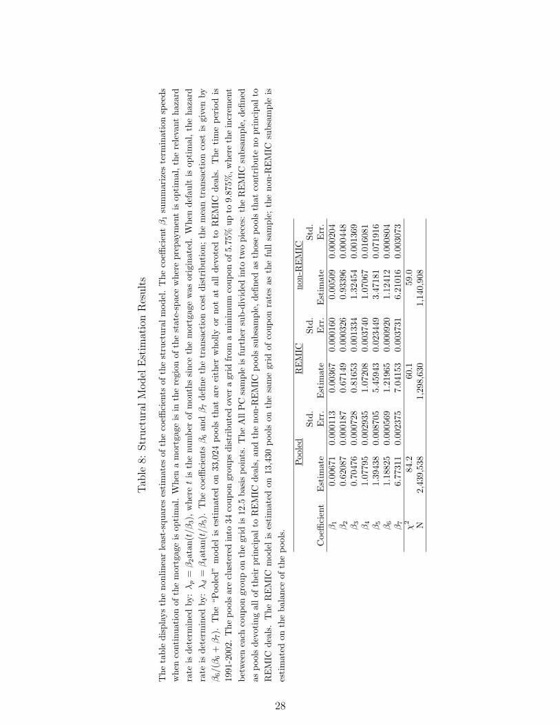
Tab
le8:
Str
uct
ura
lM
odel
Est
imat
ion
Res
ult
s
The
tabl
edi
spla
ysth
eno
nlin
ear
leas
t-sq
uare
ses
tim
ates
ofth
eco
effici
ents
ofth
est
ruct
ural
mod
el.
The
coeffi
cien
tβ
1su
mm
ariz
este
rmin
atio
nsp
eeds
whe
nco
ntin
uati
onof
the
mor
tgag
eis
opti
mal
.W
hen
am
ortg
age
isin
the
regi
onof
the
stat
e-sp
ace
whe
repr
epay
men
tis
opti
mal
,the
rele
vant
haza
rdra
teis
dete
rmin
edby
:λ
p=
β2at
an(t
/β3),
whe
ret
isth
enu
mbe
rof
mon
ths
sinc
eth
em
ortg
age
was
orig
inat
ed.
Whe
nde
faul
tis
opti
mal
,th
eha
zard
rate
isde
term
ined
by:
λd
=β
4at
an(t
/β5).
The
coeffi
cien
tsβ
6an
dβ
7de
fine
the
tran
sact
ion
cost
dist
ribu
tion
;th
em
ean
tran
sact
ion
cost
isgi
ven
byβ
6/(
β6
+β
7).
The
“Poo
led”
mod
elis
esti
mat
edon
33,0
24po
ols
that
are
eith
erw
holly
orno
tat
allde
vote
dto
RE
MIC
deal
s.T
heti
me
peri
odis
1991
-200
2.T
hepo
ols
are
clus
tere
din
to34
coup
ongr
oups
dist
ribu
ted
over
agr
idfr
oma
min
imum
coup
onof
5.75
%up
to9.
875%
,whe
reth
ein
crem
ent
betw
een
each
coup
ongr
oup
onth
egr
idis
12.5
basi
spo
ints
.T
heA
llP
Csa
mpl
eis
furt
her
sub-
divi
ded
into
two
piec
es:
the
RE
MIC
subs
ampl
e,de
fined
aspo
ols
devo
ting
allo
fth
eir
prin
cipa
lto
RE
MIC
deal
s,an
dth
eno
n-R
EM
ICpo
ols
subs
ampl
e,de
fined
asth
ose
pool
sth
atco
ntri
bute
nopr
inci
palt
oR
EM
ICde
als.
The
RE
MIC
mod
elis
esti
mat
edon
13,4
30po
ols
onth
esa
me
grid
ofco
upon
rate
sas
the
full
sam
ple;
the
non-
RE
MIC
subs
ampl
eis
esti
mat
edon
the
bala
nce
ofth
epo
ols.
Poo
led
RE
MIC
non-
RE
MIC
Std.
Std.
Std.
Coe
ffici
ent
Est
imat
eE
rr.
Est
imat
eE
rr.
Est
imat
eE
rr.
β1
0.00
671
0.00
0113
0.00
367
0.00
0160
0.00
509
0.00
0204
β2
0.62
087
0.00
0187
0.67
149
0.00
0326
0.93
396
0.00
0448
β3
0.70
476
0.00
0728
0.81
653
0.00
1334
1.32
454
0.00
1369
β4
1.07
795
0.00
2935
1.07
208
0.00
3740
1.07
067
0.01
6081
β5
1.39
438
0.00
8705
5.45
943
0.02
3449
3.47
181
0.07
1916
β6
1.18
825
0.00
0569
1.21
965
0.00
0920
1.12
412
0.00
0804
β7
6.77
311
0.00
2375
7.04
153
0.00
3731
6.21
016
0.00
3073
χ2
84.2
60.1
59.0
N2,
439,
538
1,29
8,63
01,
140,
908
28
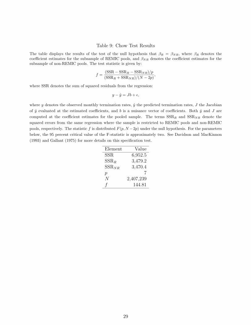
Table 9: Chow Test Results
The table displays the results of the test of the null hypothesis that βR = βNR, where βR denotes thecoefficient estimates for the subsample of REMIC pools, and βNR denotes the coefficient estimates for thesubsample of non-REMIC pools. The test statistic is given by:
f =(SSR− SSRR − SSRNR)/p
(SSRR + SSRNR)/(N − 2p),
where SSR denotes the sum of squared residuals from the regression:
y − y = Jb + ε,
where y denotes the observed monthly termination rates, y the predicted termination rates, J the Jacobianof y evaluated at the estimated coefficients, and b is a nuisance vector of coefficients. Both y and J arecomputed at the coefficient estimates for the pooled sample. The terms SSRR and SSRNR denote thesquared errors from the same regression where the sample is restricted to REMIC pools and non-REMICpools, respectively. The statistic f is distributed F (p, N −2p) under the null hypothesis. For the parametersbelow, the 95 percent critical value of the F-statistic is approximately two. See Davidson and MacKinnon(1993) and Gallant (1975) for more details on this specification test.
Element ValueSSR 6,952.5SSRR 3,479.2SSRNR 3,470.4p 7N 2,407,239f 144.81
29
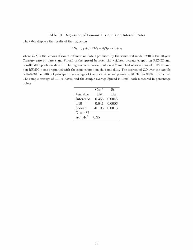
Table 10: Regression of Lemons Discounts on Interest Rates
The table displays the results of the regression
LDt = β0 + β1T10t + β2Spreadt + εt
where LDt is the lemons discount estimate on date t produced by the structural model, T10 is the 10-yearTreasury rate on date t and Spread is the spread between the weighted average coupon on REMIC andnon-REMIC pools on date t. The regression is carried out on 487 matched observations of REMIC andnon-REMIC pools originated with the same coupon on the same date. The average of LD over the sampleis $−0.064 per $100 of principal; the average of the positive lemon premia is $0.039 per $100 of principal.The sample average of T10 is 6.068, and the sample average Spread is 1.596, both measured in percentagepoints.
Coef. Std.Variable Est. Err.Intercept 0.356 0.0045T10 -0.041 0.0006Spread -0.106 0.0013N = 487Adj.-R2 = 0.95
30

Figure 1: Ownership of Freddie Mac PCs
The vertical bars in the figure display the dollar amount by year of origination of PCs sold (light bars) andheld (dark bars) by Freddie Mac. The solid line shows the ratio of PCs held to the total amount of PCsoutstanding, and is to be read against the percentages on the right axis.
0
100,000
200,000
300,000
400,000
500,000
600,000
700,000
800,000
1992 1993 1994 1995 1996 1997 1998 1999 2000 2001 2002
$ M
illio
ns
0%
5%
10%
15%
20%
25%
30%
35%
PC Sold (Left Axis) PC Held (Left Axis) PC Held/ PC Total (Right Axis)
31

Figure 2: Outstanding Balances of Freddie Mac PC’s held in REMIC and NONREMICStructures
The figure plots the outstanding balances of unseasoned Freddie Mac PCs that back REMIC securities (solidline) and non-REMIC securities (dashed line). The calculations are made for the 61,929 unseasoned poolsdisplayed in table 2 above.
$0
$50,000
$100,000
$150,000
$200,000
$250,000
Jan-91
Jan-92
Jan-93
Jan-94
Jan-95
Jan-96
Jan-97
Jan-98
Jan-99
Jan-00
Jan-01
Jan-02
Jan-03
Mill
ions
Non-REMIC Balance REMIC Balance
32
References
Akerloff, G., 1970, The market for lemons: Qualitative uncertainty and the market mecha-nism, Quarterly Journal of Economics 84, 488–487.
Bartlett, W., 1989, Mortgage-Backed Securities: Products, Analysis, Trading (Prentice Hall,Englewood Cliffs, N.J.).
Bond, E. W., 1982, A direct test of the lemons model: The market for used pickup trucks,The American Economic Review 72, 836–840.
Boot, A. W., and A. V. Thakor, 1997, The valuation of complex derivatives by majorinvestment firms: Empirical evidence, The Journal of Finance 2, 785–798.
Cox, D. R., and D. Oakes, 1984, Analysis of Survival Data (Chapman and Hall, New York).
Cox, J. C., J. E. Ingersoll, and S. A. Ross, 1985, A theory of the term structure of interestrates, Econometrica 53, 386–407.
Davidson, R., and J. G. MacKinnon, 1993, Estimation and Inference in Econometrics (Ox-ford University Press, New York, NY).
DeMarzo, P., 2003, The pooling and tranching of securities, forthcoming in Review of Fi-nancial Studies.
DeMarzo, P., and D. Duffie, 1998, A liquidity based model of security design, Econometrica49, 67–99.
Diamond, D. W., and R. E. Verrecchia, 1991, Disclosure, liquidity, and the cost of capital,Journal of Finance 1325–1359.
Downing, C., R. Stanton, and N. Wallace, 2005, An empirical test of a two-factor mort-gage valuation model: How much do house prices matter?, forthcoming in Real EstateEconomics.
Gallant, A. R., 1975, Nonlinear regression, The American Statistician 29, 73–81.
Glaeser, E., and H. D. Kallal, 1997, Thin markets, asymmetric information, and mortgagebacked securities, Journal of Financial Intermediation 6, 64–86.
Gorton, G., and G. Pennachi, 1990, Financial intermediaries and liquidity creation, Journalof Finance 45, 45–71.
Kalbfleisch, J. D., and R. L. Prentice, 1980, The Statistical Analysis of Failure Time Data(John Wiley, New York).
Kau, J. B., D. C. Keenan, W. J. Muller, and J. F. Epperson, 1992, A generalized valuationmodel for fixed-rate residential mortgages, Journal of Money, Credit and Banking 24,279–299.
33
Kau, J. B., D. C. Keenan, W. J. Muller, III, and J. F. Epperson, 1995, The valuation atorigination of fixed rate mortgages with default and prepayment, Journal of Real EstateFinance and Economics 11, 5–39.
Merton, R. C., 1973, Theory of rational option pricing, Bell Journal of Economics andManagement Science 4, 141–183.
Oldfield, G., 2000, Making markets for structure derivatives, Journal of Financial Economics57, 445–471.
Pearson, N. D., and T.-S. Sun, 1989, A test of the Cox, Ingersoll, Ross model of the termstructure of interest rates using the method of maximum likelihood, Working paper, MIT.
Richard, S. F., and R. Roll, 1989, Prepayments on fixed rate mortgage-backed securities,Journal of Portfolio Management 15, 73–82.
Stanton, R., 1995, Rational prepayment and the value of mortgage-backed securities, TheReview of Financial Studies 8, 677–708.
United States Department of the Treasury, 2003, Enhancing disclosure in the mortgage-backed securities markets, Staff report, Task Force on Mortgage Backed Securities.
34