


Individual dynamic predictions usinglandmarking and joint modelling: validation of
estimators and robustness assessment
Loïc Ferrer1,†, Hein Putter2 and Cécile Proust-Lima1
(1)Biostatistics Team, INSERM U1219, University of Bordeaux, Bordeaux, France(2)Department of Medical Statistics and Bioinformatics, Leiden University Medical Center,
Leiden, The Netherlands(†)email : [email protected]
Journées GDR/SFB
ISPED, Université de Bordeaux, France
October 05, 2017
Introduction Prediction models Accuracy / Robustness Discussion
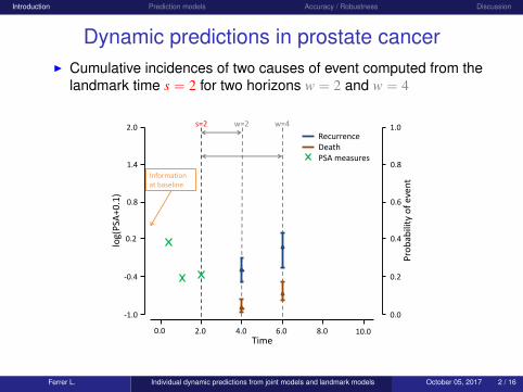
Dynamic predictions in prostate cancerI Cumulative incidences of two causes of event computed from the
landmark time s = 2 for two horizons w = 2 and w = 4
0.0 2.0 8.06.04.0 10.0Time
0.0
0.2
0.4
0.6
0.8
1.0
-1.0
-0.4
0.2
0.8
1.4
2.0
log(
PSA
+0.1
)
Pro
bab
ility
of
even
t
s=2 w=2 w=4
Information at baseline
RecurrenceDeathPSA measures
Ferrer L. Individual dynamic predictions from joint models and landmark models October 05, 2017 2 / 16

Introduction Prediction models Accuracy / Robustness Discussion
Dynamic predictions in prostate cancerI Cumulative incidences of two causes of event computed from the
landmark time s = 4 for two horizons w = 2 and w = 4
0.0 2.0 8.06.04.0 10.0Time
0.0
0.2
0.4
0.6
0.8
1.0
-1.0
-0.4
0.2
0.8
1.4
2.0lo
g(P
SA+0
.1)
Pro
bab
ility
of
even
t
RecurrenceDeathPSA measures
s=4 w=2 w=4
Information at baseline
Ferrer L. Individual dynamic predictions from joint models and landmark models October 05, 2017 2 / 16
Introduction Prediction models Accuracy / Robustness Discussion
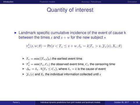
Quantity of interest
I Landmark specific cumulative incidence of the event of cause kbetween the times s and s + w for the new subject ?
πk?(s,w; θ) = Pr(s < T? ≤ s + w, δ? = k|T? > s,Y?(s),X?; θ)
I T? = min({T?,k}k) the earliest event time
I T†? = min(T?,C?) the observed event time, C? the censoring timeI ∆? = δ? .1{T? ≤ C?}, where δ? = k is the cause of eventI Y?(s) and X? the individual information collected until s
Ferrer L. Individual dynamic predictions from joint models and landmark models October 05, 2017 3 / 16

Introduction Prediction models Accuracy / Robustness Discussion
Objectives
I When Y?(s) includes internal time-dependent covariates⇒needs to handle the dependency between Y? and (T?, δ?)
I Joint modellingI Landmarking
• Cause-specific PH models• Pseudo-observations approach
=⇒ Validation of the estimators from the joint and landmark modelsand their uncertainty
=⇒ Comparison of the joint and landmark models in terms ofprediction accuracy and robustness to the model hypotheses
Ferrer L. Individual dynamic predictions from joint models and landmark models October 05, 2017 4 / 16

Introduction Prediction models Accuracy / Robustness Discussion
Joint modelI Information O used in the learning step: Whole information
O = {(T†i ,∆i,Yi(T†i ),Xi)}i=1,...,N
I Model formulationYi(t) = Y∗i (t) + εi(t)
= XLi (t)>β + Zi(t)>bi + εi(t)
λki (t) = λk,0(t) exp
{XE >
k,i γk + Wk,i(t|bi;β,D)>ηk}
I bi ∼ N (0,D) ; εi ∼ N (0, σ2Ini ) ; λ0,k(.) the param. baseline hazard
I Cumulative incidence estimator for new subject ?
πk?(s,w; θ) =
∫Rqπk?(s,w|b?; θ) f (b?|T? > s,Y?(s),X?; θ) db?
I f (.) a probability density function
Ferrer L. Individual dynamic predictions from joint models and landmark models October 05, 2017 5 / 16
Introduction Prediction models Accuracy / Robustness Discussion
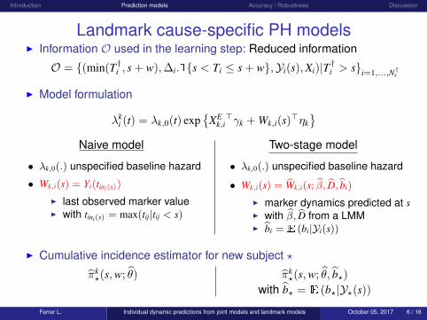
Landmark cause-specific PH modelsI Information O used in the learning step: Reduced information
O = {(min(T†i , s + w),∆i.1{s < Ti ≤ s + w},Yi(s),Xi)|T†i > s}i=1,...,N†s
I Model formulation
λki (t) = λk,0(t) exp
{XE >
k,i γk + Wk,i(s)>ηk}
Naive model
• λk,0(.) unspecified baseline hazard
• Wk,i(s) = Yi(tini(s))
I last observed marker valueI with tini(s) = max(tij|tij < s)
Two-stage model
• λk,0(.) unspecified baseline hazard
• Wk,i(s) = Wk,i(s; β, D, bi)
I marker dynamics predicted at sI with β, D from a LMMI bi = E (bi|Yi(s))
I Cumulative incidence estimator for new subject ?
πk?(s,w; θ) πk
?(s,w; θ, b?)
with b? = E (b?|Y?(s))
Ferrer L. Individual dynamic predictions from joint models and landmark models October 05, 2017 6 / 16
Introduction Prediction models Accuracy / Robustness Discussion
Two-stage landmark pseudo-values approachI Information O used in the learning step: Reduced information
O = {(T†i ,∆i,Yi(s),Xi)|T†i > s}i=1,...,N†s
I Model formulation
g[E{µk
i,s,w|T†i > s}
]= γ0 + XE >
k,i γ1 + Wk,i(s; β, D, bi)>η
I where the dynamic pseudo-observation is
µki,s,w = NsFk(s,w)− (Ns − 1)Fk
(−i)(s,w)
• Ns =∑
i1{T∗i > s}, Fk(s,w) non-par. estimator of πk(s,w)
I Cumulative incidence estimator for new subject ? (g(x) = cloglog(x))
πk?(s,w; θ, b?) = 1− exp
[− exp{γ0 + XE >
k,? γ1 + Wk,?(s; β, D, b?)>η}]
Ferrer L. Individual dynamic predictions from joint models and landmark models October 05, 2017 7 / 16
Introduction Prediction models Accuracy / Robustness Discussion
Prediction accuracy / Robustness
I Comparison of the joint and landmark models in terms ofI Prediction errorI Discriminatory powerI Robustness to the model hypotheses
I 4 scenariiI Well-specification of the joint modelI Misspecification of the dependence functionI Violation of the PH assumptionI Misspecification of the longitudinal trend of the marker
Ferrer L. Individual dynamic predictions from joint models and landmark models October 05, 2017 8 / 16

Introduction Prediction models Accuracy / Robustness Discussion
Tools for comparisonI For each scenario, data generated from JM→ For each new subject ? = 1, . . . ,Nnew
s (Nnew0 = 500)
πk?(s,w; θ) =
∫Rq
πk?(s,w|b?; θ) f (b?|T? > s,Y?(s),X?; θ) db?
I For each replicate r = 1, . . . , 500 and each ? = 1, . . . ,Nnews
→ πk?,r(s,w; θ) computed using JM, Naive-LM-PH, 2s-LM-PH
and 2s-LM-PV approaches
I Comparison between the prediction models using boxplots of thedifferences of Mean Square Error of Prediction (MSEP) over the500 replicates, where
MSEPkr(s,w) =
1Nnew
s
Nnews∑
?=1
(πk?(s,w; θ)− πk
?,r(s,w; θ))2× 1000
Ferrer L. Individual dynamic predictions from joint models and landmark models October 05, 2017 9 / 16
Introduction Prediction models Accuracy / Robustness Discussion
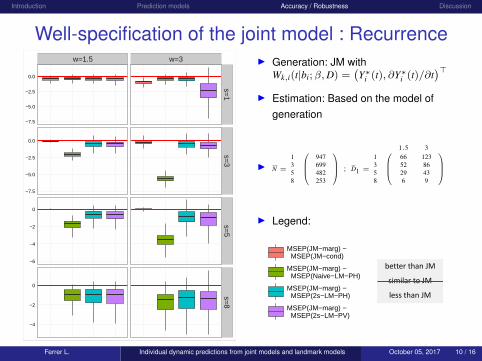
Well-specification of the joint model : Recurrencew=1.5 w=3
−7.5
−5.0
−2.5
0.0
s=1
−7.5
−5.0
−2.5
0.0
s=3
−6
−4
−2
0
s=5
−4
−2
0
s=8
I Generation: JM withWk,i(t|bi;β,D) =
(Y∗i (t), ∂Y∗i (t)/∂t
)>I Estimation: Based on the model of
generation
I N =
1 9473 6995 4828 253
; D1 =
1.5 3
1 66 1233 52 865 29 438 6 9
I Legend:
MSEP(JM−marg) − MSEP(JM−cond)
MSEP(JM−marg) − MSEP(Naive−LM−PH)
MSEP(JM−marg) − MSEP(2s−LM−PH)
MSEP(JM−marg) − MSEP(2s−LM−PV)
better than JM
similar to JM
less than JM
Ferrer L. Individual dynamic predictions from joint models and landmark models October 05, 2017 10 / 16

Introduction Prediction models Accuracy / Robustness Discussion
Misspecification of the dependence function: Rec.w=1.5 w=3
−2
−1
0
1
s=1
−6
−4
−2
0
s=3
−4
−2
0
s=5
−5.0
−2.5
0.0
2.5
s=8
I Generation: JM withWk,i(t|bi;β,D) =
(Y∗i (t), ∂Y∗i (t)/∂t
)>I Estimation: JM, 2s-LM-PH and
2s-LM-PV using Wk,i(t|bi;β,D) = Y∗i (t)
I N =
1 9473 6995 4828 253
; D1 =
1.5 3
1 66 1233 52 865 29 438 6 9
I Legend:
MSEP(JM−marg) − MSEP(JM−cond)
MSEP(JM−marg) − MSEP(Naive−LM−PH)
MSEP(JM−marg) − MSEP(2s−LM−PH)
MSEP(JM−marg) − MSEP(2s−LM−PV)
better than JM
similar to JM
less than JM
Ferrer L. Individual dynamic predictions from joint models and landmark models October 05, 2017 11 / 16

Introduction Prediction models Accuracy / Robustness Discussion
Violation of the PH assumption: Rec.w=1.5 w=3
−30
−20
−10
0
s=1
−20
−15
−10
−5
0
s=3
−20
−15
−10
−5
0
5
s=5
−20
−10
0
s=8
I Generation: JM with interaction of ηk withlog(1 + t)
I Estimation: By neglecting log(1 + t)
I N =
1 9653 6895 4228 199
; D1 =
1.5 3
1 76 1833 101 1625 48 718 9 14
I Legend:
MSEP(JM−marg) − MSEP(JM−cond)
MSEP(JM−marg) − MSEP(Naive−LM−PH)
MSEP(JM−marg) − MSEP(2s−LM−PH)
MSEP(JM−marg) − MSEP(2s−LM−PV)
better than JM
similar to JM
less than JM
Ferrer L. Individual dynamic predictions from joint models and landmark models October 05, 2017 12 / 16
Introduction Prediction models Accuracy / Robustness Discussion
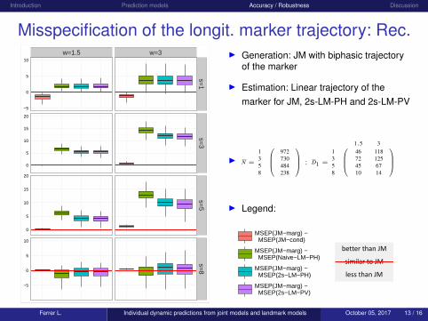
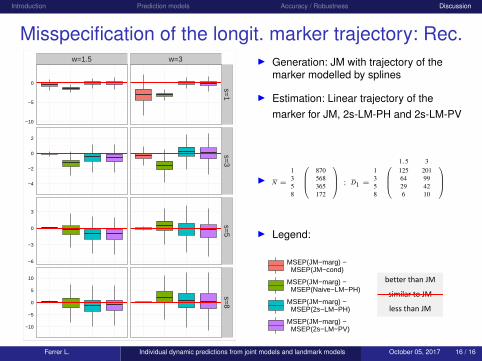
Misspecification of the longit. marker trajectory: Rec.w=1.5 w=3
−5
0
5
10
s=1
0
5
10
15
20
s=3
0
5
10
15
20
s=5
−5
0
5
10
s=8
I Generation: JM with biphasic trajectoryof the marker
I Estimation: Linear trajectory of themarker for JM, 2s-LM-PH and 2s-LM-PV
I N =
1 9723 7305 4848 238
; D1 =
1.5 3
1 46 1183 72 1255 45 678 10 14
I Legend:
MSEP(JM−marg) − MSEP(JM−cond)
MSEP(JM−marg) − MSEP(Naive−LM−PH)
MSEP(JM−marg) − MSEP(2s−LM−PH)
MSEP(JM−marg) − MSEP(2s−LM−PV)
better than JM
similar to JM
less than JM
Ferrer L. Individual dynamic predictions from joint models and landmark models October 05, 2017 13 / 16

Introduction Prediction models Accuracy / Robustness Discussion
Discussion (1/2)
I Accuracy/RobustnessI JM better than LM when well-specifiedI JM better than LM when misspecification of the association
function but much worse performances for both in terms of PEI JM & LM comparable when strong violation of the PH assumptionI LM better than JM when strong misspecification of the longitudinal
marker trajectory
I Discriminatory powerI AUC examinationsI yet sometimes to a lesser extent probably explained by the lesser
sensitivity of AUC and the possibly preserved discriminatory powerin the presence of worse calibration
Ferrer L. Individual dynamic predictions from joint models and landmark models October 05, 2017 14 / 16

Introduction Prediction models Accuracy / Robustness Discussion
Discussion (2/2)
I Validation of the estimators and their variabilityI Good individual coverage rates of cumulative incidences for
two-stage landmark CS PH model and joint modelI Individual relative bias→ JM unbiased, LM biased in earlier
landmark timesI Length of the individual 95% confidence intervals→ estimator
more efficient using JM than LM
I Implementation in RI JM with extensions for joint modellingI mstate for cause-specific modellingI pseudo and geepack for dynamic pseudo-values approach
Ferrer L. Individual dynamic predictions from joint models and landmark models October 05, 2017 15 / 16
Introduction Prediction models Accuracy / Robustness Discussion
ReferencesI Blanche, P., Proust-Lima, C., Loubère, L., Berr, C., Dartigues, J.-F., and Jacqmin-Gadda, H.
(2015). Quantifying and comparing dynamic predictive accuracy of joint models for
longitudinal marker and time-to-event in presence of censoring and competing risks.
Biometrics, 71(1):102–113.
I Ferrer, L., Putter, H., & Proust-Lima, C. (available on request). Individual dynamic predictions
using landmarking and joint modelling: validation of estimators and robustness assessment.
I Maziarz, M., Heagerty, P., Cai, T., & Zheng, Y. (2016). On longitudinal prediction with
time-to-event outcome: Comparison of modeling options. Biometrics.
I Nicolaie, M. A., van Houwelingen, J. C., de Witte, T. M., and Putter, H. (2013). Dynamic
Pseudo-Observations: A Robust Approach to Dynamic Prediction in Competing Risks.
Biometrics, 69(4):1043–1052.
I Proust-Lima, C., & Blanche, P. (2015). Dynamic Predictions. In /WileyStatsRef: Statistics
Reference Online/. John Wiley & Sons, Ltd.
I Rizopoulos, D. (2011). Dynamic predictions and prospective accuracy in joint models for
longitudinal and time-to-event data. Biometrics, 67(3):819–29.
I van Houwelingen, H. and Putter, H. (2011). Dynamic Prediction in Clinical Survival Analysis.
Monographs on Statistics & Applied Probab #123. Chapman & Hall/CRC, London.
Ferrer L. Individual dynamic predictions from joint models and landmark models October 05, 2017 16 / 16
Introduction Prediction models Accuracy / Robustness Discussion
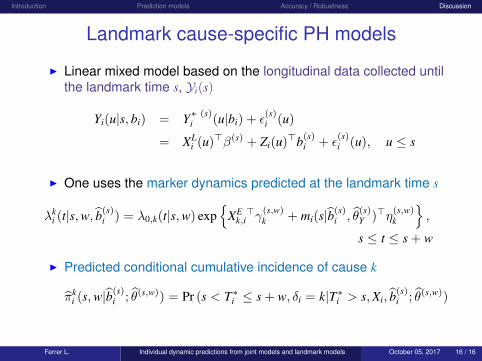
Landmark cause-specific PH models
I Linear mixed model based on the longitudinal data collected untilthe landmark time s, Yi(s)
Yi(u|s, bi) = Y∗ (s)i (u|bi) + ε
(s)i (u)
= XLi (u)>β(s) + Zi(u)>b(s)
i + ε(s)i (u), u ≤ s
I One uses the marker dynamics predicted at the landmark time s
λki (t|s,w, b(s)
i ) = λ0,k(t|s,w) exp{
XE >k,i γ
(s,w)k + mi(s|b(s)
i , θ(s)Y )>η
(s,w)k
},
s ≤ t ≤ s + w
I Predicted conditional cumulative incidence of cause k
πki (s,w|b(s)
i ; θ(s,w)) = Pr (s < T∗i ≤ s + w, δi = k|T∗i > s,Xi, b(s)i ; θ(s,w))
Ferrer L. Individual dynamic predictions from joint models and landmark models October 05, 2017 16 / 16
Introduction Prediction models Accuracy / Robustness Discussion
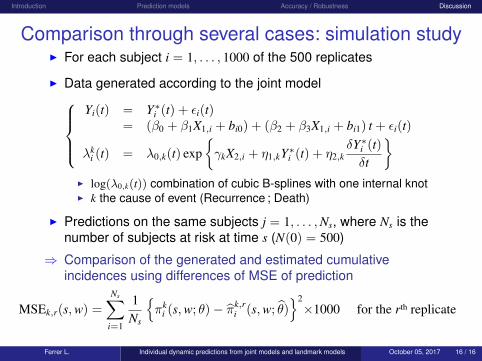
Comparison through several cases: simulation studyI For each subject i = 1, . . . , 1000 of the 500 replicates
I Data generated according to the joint modelYi(t) = Y∗i (t) + εi(t)
= (β0 + β1X1,i + bi0) + (β2 + β3X1,i + bi1) t + εi(t)
λki (t) = λ0,k(t) exp
{γkX2,i + η1,kY∗i (t) + η2,k
δY∗i (t)δt
}I log(λ0,k(t)) combination of cubic B-splines with one internal knotI k the cause of event (Recurrence ; Death)
I Predictions on the same subjects j = 1, . . . ,Ns, where Ns is thenumber of subjects at risk at time s (N(0) = 500)
⇒ Comparison of the generated and estimated cumulativeincidences using differences of MSE of prediction
MSEk,r(s,w) =
Ns∑i=1
1Ns
{πk
i (s,w; θ)− πk,ri (s,w; θ)
}2×1000 for the rth replicate
Ferrer L. Individual dynamic predictions from joint models and landmark models October 05, 2017 16 / 16
Introduction Prediction models Accuracy / Robustness Discussion
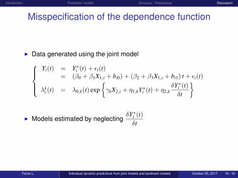
Misspecification of the dependence function
I Data generated using the joint modelYi(t) = Y∗i (t) + εi(t)
= (β0 + β1X1,i + bi0) + (β2 + β3X1,i + bi1) t + εi(t)
λki (t) = λ0,k(t) exp
{γkX2,i + η1,kY∗i (t) + η2,k
δY∗i (t)δt
}
I Models estimated by neglectingδY∗i (t)δt
Ferrer L. Individual dynamic predictions from joint models and landmark models October 05, 2017 16 / 16
Introduction Prediction models Accuracy / Robustness Discussion
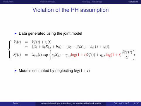
Violation of the PH assumption
I Data generated using the joint modelYi(t) = Y∗i (t) + εi(t)
= (β0 + β1X1,i + bi0) + (β2 + β3X1,i + bi1) t + εi(t)
λki (t) = λ0,k(t) exp
{γkX2,i + η1,klog(1 + t)Y∗i (t) + η2,klog(1 + t)
δY∗i (t)δt
}
I Models estimated by neglecting log(1 + t)
Ferrer L. Individual dynamic predictions from joint models and landmark models October 05, 2017 16 / 16

Introduction Prediction models Accuracy / Robustness Discussion
Comparison between η1,Rec. × log(1 + t) and η1,Rec.1st replicate
0
1
2
0 5 10 15Time
Par
amet
er
Method
True
JM
LM CSPH (w=1.5)
LM CSPH (w=3)
Ferrer L. Individual dynamic predictions from joint models and landmark models October 05, 2017 16 / 16

Introduction Prediction models Accuracy / Robustness Discussion
Comparison between η1,Death × log(1 + t) and η1,Death1st replicate
−0.5
0.0
0.5
1.0
0 5 10 15Time
Par
amet
er
Method
True
JM
LM CSPH (w=1.5)
LM CSPH (w=3)
Ferrer L. Individual dynamic predictions from joint models and landmark models October 05, 2017 16 / 16
Introduction Prediction models Accuracy / Robustness Discussion
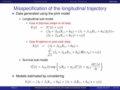
Misspecification of the longitudinal trajectoryI Data generated using the joint model
I Longitudinal sub-model• Case A (biphasic shape on all data)
Yi(t) = Y∗i (t) + εi(t)= (β0 + β0,XX1,i + bi0) + (β1 + β1,XX1,i + bi1) f1(t)+
(β2 + β2,XX1,i + bi2) t + εi(t)
• Case B (splines on post-nadir data)
Yi(t) = (β0 + β0,XX1,i + bi0) +3∑
p=1(βp + βp,XX1,i + bip) B(t, κp) + εi(t)
I Survival sub-model
λki (t) = λ0,k(t) exp
{γkX2,i + η1,kY∗i (t) + η2,k
δY∗i (t)δt
}I Models estimated by considering
Yi(t) = (β0 + β1X1,i + bi0) + (β2 + β3X1,i + bi1) t + εi(t)
Ferrer L. Individual dynamic predictions from joint models and landmark models October 05, 2017 16 / 16
Introduction Prediction models Accuracy / Robustness Discussion
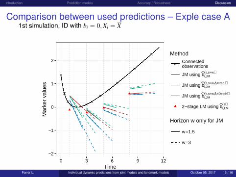
Comparison between used predictions – Exple case A1st simulation, ID with bi = 0,Xi = X
−2
−1
0
1
2
0 3 6 9 12Time
Mar
ker
valu
es
MethodConnected observations
JM using bi,JM(s,s+w)
JM using bi,JM(s,s+w,δi=Rec.)
JM using bi,JM(s,s+w,δi=Death)
2−stage LM using bi,LM(s)
Horizon w only for JM
w=1.5
w=3
Ferrer L. Individual dynamic predictions from joint models and landmark models October 05, 2017 16 / 16
Introduction Prediction models Accuracy / Robustness Discussion
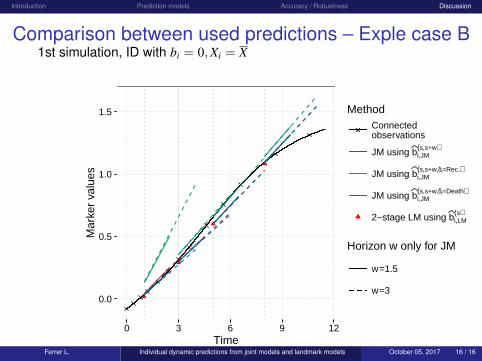
Comparison between used predictions – Exple case B1st simulation, ID with bi = 0,Xi = X
0.0
0.5
1.0
1.5
0 3 6 9 12Time
Mar
ker
valu
es
MethodConnected observations
JM using bi,JM(s,s+w)
JM using bi,JM(s,s+w,δi=Rec.)
JM using bi,JM(s,s+w,δi=Death)
2−stage LM using bi,LM(s)
Horizon w only for JM
w=1.5
w=3
Ferrer L. Individual dynamic predictions from joint models and landmark models October 05, 2017 16 / 16
Introduction Prediction models Accuracy / Robustness Discussion
Misspecification of the longit. marker trajectory: Rec.w=1.5 w=3
−10
−5
0 s=1
−4
−2
0
2
s=3
−6
−3
0
3
s=5
−10
−5
0
5
10
s=8
I Generation: JM with trajectory of themarker modelled by splines
I Estimation: Linear trajectory of themarker for JM, 2s-LM-PH and 2s-LM-PV
I N =
1 8703 5685 3658 172
; D1 =
1.5 3
1 125 2013 64 995 29 428 6 10
I Legend:
MSEP(JM−marg) − MSEP(JM−cond)
MSEP(JM−marg) − MSEP(Naive−LM−PH)
MSEP(JM−marg) − MSEP(2s−LM−PH)
MSEP(JM−marg) − MSEP(2s−LM−PV)
better than JM
similar to JM
less than JM
Ferrer L. Individual dynamic predictions from joint models and landmark models October 05, 2017 16 / 16

Introduction Prediction models Accuracy / Robustness Discussion
First objective
I Validation of the proposed estimators and their uncertainty
⇒ Simulation study with focus on the bias and coverage ratesI Data generated according to a joint model⇒ For each new subject ? = 1, . . . ,Nnew
s (Nnew0 = 500)
πk?(s,w; θ) =
∫Rq
πk?(s,w|b?; θ) f (b?|T? > s,Y?(s),X?; θ) db?
I For each replicate r = 1, . . . , 500 and each ? = 1, . . . ,Nnews
→ πk?,r(s,w; θ) computed using JM, Naive-LM-PH,
2s-LM-PH and 2s-LM-PV approaches
Ferrer L. Individual dynamic predictions from joint models and landmark models October 05, 2017 16 / 16

Introduction Prediction models Accuracy / Robustness Discussion
Validation of the estimators and their uncertainty
I Interest in the distribution over the subjects of the relative bias(RB) of πk
?(s,w; θ)
RBk?(s,w) =
1R
R∑r=1
πk?,r(s,w; θ)− πk
?(s,w; θ)
πk?(s,w; θ)
I Interest in the distribution over the subjects of the coverage rates(COV)
COVk?(s,w) =
1R
R∑r=1
(πk?(s,w; θ) ∈
[q0.025{πk,(l)
?,r (s,w; θ(l)); l = 1, . . . ,L};
q0.975{πk,(l)?,r (s,w; θ(l)); l = 1, . . . ,L}
])I Results obtained for R = 500 replicates, Nnew
0 = 500
Ferrer L. Individual dynamic predictions from joint models and landmark models October 05, 2017 16 / 16

Introduction Prediction models Accuracy / Robustness Discussion
Relative bias
I Distribution over the subjects of the relative bias (RB) ofπk?(s,w; θ)
s=1, w=3
−40
0
40
80
s=5, w=3
−40
0
40
80
RB(JM−marg) RB(JM−cond) RB(2s−LM−PH)
Ferrer L. Individual dynamic predictions from joint models and landmark models October 05, 2017 16 / 16
Introduction Prediction models Accuracy / Robustness Discussion
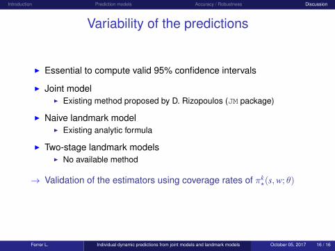
Variability of the predictions
I Essential to compute valid 95% confidence intervals
I Joint modelI Existing method proposed by D. Rizopoulos (JM package)
I Naive landmark modelI Existing analytic formula
I Two-stage landmark modelsI No available method
→ Validation of the estimators using coverage rates of πk?(s,w; θ)
Ferrer L. Individual dynamic predictions from joint models and landmark models October 05, 2017 16 / 16
Introduction Prediction models Accuracy / Robustness Discussion
Confidence intervals of the predictions from JMParametric bootstrap: for each l = 1, . . . ,L
1. Generate θ(l) ∼ N (θ, V(θ))
2. 2 solutions: compute πk,(l)? (s,w; θ(l)) using
a. either the conditional probability
πk,(l)? (s,w; θ(l), b(l)
? )
• where b(l)? = arg max
bf (b|T? > s,Y?(s),X?; θ(l))
b. or the marginal probability∫Rqπ
k,(l)? (s,w|b?; θ(l)) db?
=⇒ Deduce 95% confidence interval[q0.025{πk,(l)
? (s,w; θ(l)); l = 1, . . . ,L} ; q0.975{πk,(l)? (s,w; θ(l)); l = 1, . . . ,L}
]Ferrer L. Individual dynamic predictions from joint models and landmark models October 05, 2017 16 / 16

Introduction Prediction models Accuracy / Robustness Discussion
Confidence intervals of the predictions from 2s-LM-PH
Parametric bootstrap [1.] and perturbation-resampling [2.]
For each l = 1, . . . ,L
1. Generate θ(l) ∼ N (θ, V(θ))
I b(l)i = E(bi|Yi(s); θ(l)) and b(l)
? = E(b?|Y?(s); θ(l))
2. a. Perturb the observed time-to-event data: for i = 1, . . . ,Ns
• νi ∼ 4 · Beta( 12 ,
32 )
• T∗i = νi · T∗i ; ∆i = νi ·∆i
b. Update the Breslow-estimator Λ(l)k,0(.) = f (θ(l), {b(l)
i , T∗i , ∆i}i=1,...,Ns )
3. Compute πk,(l)? (s,w; θ(l)) = f (Λ
(l)k,0(.), θ(l), b(l)
? )
=⇒ Deduce the 95% confidence interval[q0.025{πk,(l)
? (s,w; θ(l)); l = 1, . . . ,L} ; q0.975{πk,(l)? (s,w; θ(l)); l = 1, . . . ,L}
]Ferrer L. Individual dynamic predictions from joint models and landmark models October 05, 2017 16 / 16
Introduction Prediction models Accuracy / Robustness Discussion
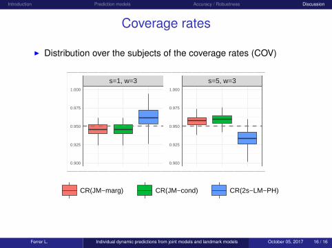
Coverage rates
I Distribution over the subjects of the coverage rates (COV)
s=1, w=3
0.900
0.925
0.950
0.975
1.000
s=5, w=3
0.900
0.925
0.950
0.975
1.000
CR(JM−marg) CR(JM−cond) CR(2s−LM−PH)
Ferrer L. Individual dynamic predictions from joint models and landmark models October 05, 2017 16 / 16


![arXiv:1404.7625v1 [stat.CO] 30 Apr 2014capabilities to derive dynamic predictions for both outcomes, it allows to combine predictions from di erent models using innovative Bayesian](https://static.cupdf.com/doc/110x72/5fd403109dd11e572e2deb42/arxiv14047625v1-statco-30-apr-2014-capabilities-to-derive-dynamic-predictions.jpg)


