Improving the Representation of Maritime Transport in the EXIOBASE MRIO Dataset
Jørgen Westrum Thorsen
Master in Industrial Ecology
Supervisor: Anders Hammer Strømman, EPT
Department of Energy and Process Engineering
Submission date: June 2013
Norwegian University of Science and Technology


1
"It was with a happy heart that the good Odysseus spread his sail to catch the wind and used
his seamanship to keep his boat straight with the steering-oar"
-Homer

2
3
Abstract This aim of this report is to improve the EXIOBASE dataset by integrating life cycle
inventories of 11 individual ship classes. The report then calculated the Global Warming
Potential (GWP) of seagoing transport was calculated using Environmentally Extended Multi-
Regional Input-Output(EE MRIO) analysis. This work has made it possible to more
accurately model the GWP of interregional seagoing transport, and to assess the impact
contribution of each vessels, both for total interregional transport and as a product of the
import demand of one or more regions.
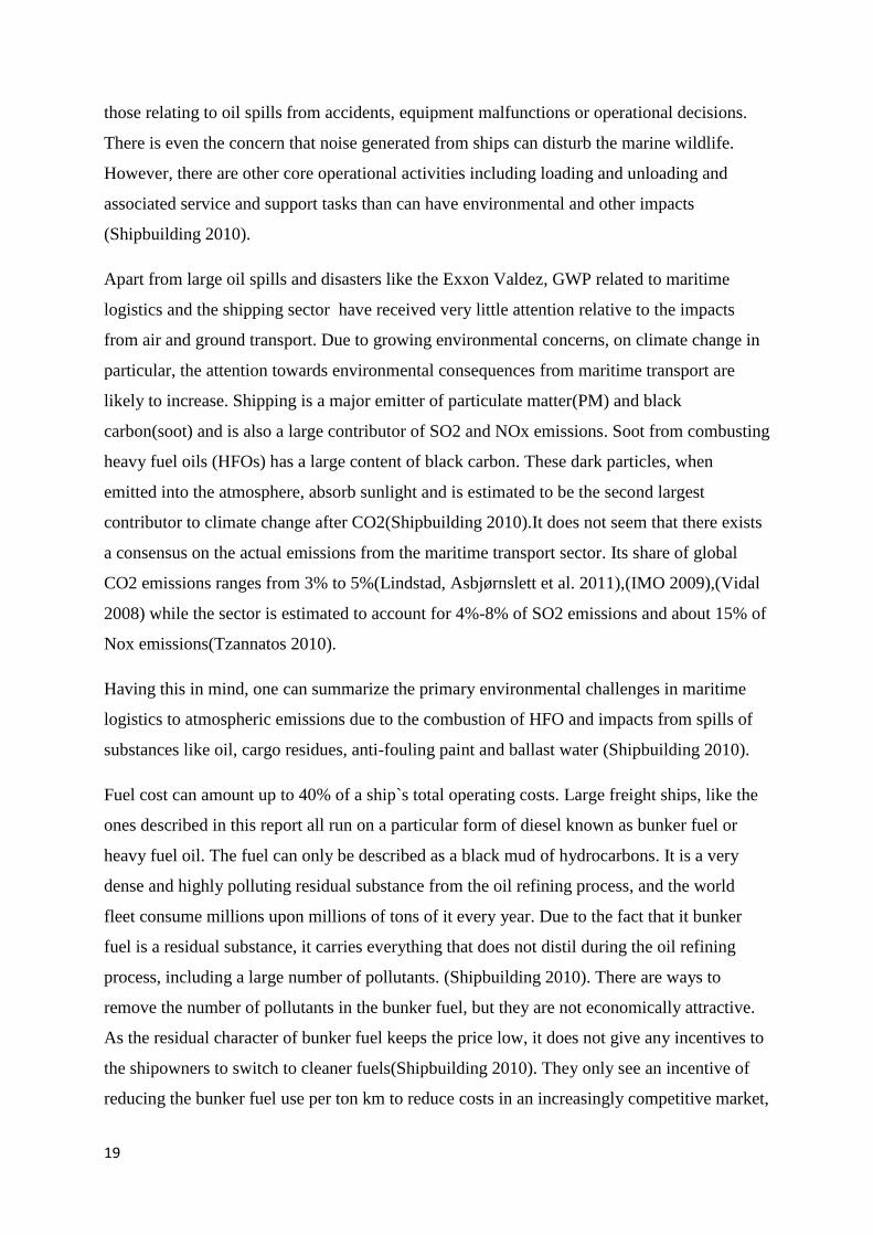
The report found that the total GWP from international maritime trade is 2.006 billion tons of
CO2-equivalents, a figure that is approximately twice as large than the ones found in similar
studies(IMO 2009, Lindstad, Asbjørnslett et al. 2012, UNCTAD 2012).
The results of this report demonstrate that North America, OECD Europe and OECD Pacific
have the highest GWP embodied in imports from seagoing trade. Crude oil carriers is the
vessel class with the largest GWP, accounting for 40% of the total fleet GWP and with OECD
Europe and North America as the greatest crude oil importers.
Figure 1 GWP by vessel type (million ton CO2-eq)
Keywords : Maritime transport, GWP, EXIOBASE, EE MRIO,

4
Acknowledgements
First, I want to thank my supervisor, arguably the busiest man in Norwegian academia,
Professor Anders Hammer Strømman for his support, enthusiasm and “big picture”-
guidance.
I also want to thank my co-supervisors, PhD Haakon Lindstad and Senior Researcher
Richard Wood for their invaluable expertise, patience and ability to answer my low-brow
questions in a non-condescending manner. My thanks is also directed at the rest of the staff
of the Industrial Ecology program for their support.
With this, six years at NTNU comes to and end. The last two years have been a great
experience with a lot of hard work, new perspectives and fun times with the fellow IndEcol-
students. Big thanks to the crew, Felipe, Sarah, Magnus, Hyun and Ty for all the good
times. To Samantha, for your companionship and your ability to make me focus on the
important things.
To Kine, Karoline, Eivind, Eirik, Stina, Elisa, Lotte and Elin, thanks for the best time in
my life so far. You rock!
The biggest thanks goes to my family, and my parents, Haakon, Bente and Bjørn for your
support, both emotionally and financially, and for teaching me to think big and work hard. To
Christoffer and my brother Herman, my closest friends. Tor Westrum, grandfather and my
greatest role model.
5
Table of Contents
Abstract 3
Acknowledgements 4
Table of Tables 7
Table of Figures 8
1 Introduction 9
2 Technology Overview 11
2.1 International Seaborne Trade 11
2.2 World fleet structure and principal vessel types 15
2.2.1 Dry Bulk 15
2.2.2 General Cargo 16
2.2.3 Tank 17
2.2.4 Ship registration and Ship owning 18
2.3 Environmental impacts related to shipping 18
3 Methodology 21
3.1 Life Cycle Assessment 21
3.1.1 What is LCA? 21
3.1.2 Goal and Scope 22
3.1.3 Life cycle Inventory(LCI) 22
3.1.4 Impact Categories 22
3.2 EEIO-MRIO 25
3.2.1 EXIOBASE 26
3.2.2 Emissions Embodied in Trade (EET) 27
4 System Description 29
4.1 Maritime Transportation 29
4.1.1 Flowchart of vessels 30
4.1.2 Techincal vessel data 31
4.1.3 Vessel emission intensities 36
4.2 EE MRIO EXIOBASE 36
4.2.1 The A-matrix 39
4.2.2 The Z-matrix 43
4.3 Global Warming Potential of International Maritime transport 45
6
5 Results 47
5.1 Total Tradeflows € 47
5.2 Shipped tradeflow € 49
5.2.1 Total trade flows shipped between regions 49
5.2.2 Total trade flows between regions, vessel resolution 51
5.3 Total ton kilometer transport 53
5.3.1 Ton kilometer transport between regions 53
5.3.2 Ton kilometer Maritime Transport, Vessel Resolution 56
5.4 Environmental Impacts 58
5.4.1 Total Global Warming Potential 58
5.4.2 Global Warming Potential from Maritime Transport 60
5.4.3 Global Warming Potential embodied in trade, vessel resolution 62
5.4.4 GWP from Maritime Transportation vs Total GWP 65
6 Discussion 67
7 Conclusion 71
7.1 Quality of data 71
7.2 Further study 72
8 References 73
9 Appendix 75
7
Table of Tables
Table 1 Freight work by vessel type (billion ton km) 13
Table 2 Overview of the midpoint categories and characterisation factors 24
Table 3 Overview of vessel data 31
Table 4 € cost per ton km transport by vessel type 32
Table 5 overview of LSW, Hull wheight and propeller wheight by vessel type 32
Table 6 Material requirements per vessel type 33
Table 7 Material requirements per ton km by vessel type 34
Table 8 € cost of material requirements per ton km by vessel type 34
Table 9 € cost per ton material 34
Table 10 € cost of material per € transport by vessel type 35
Table 11 CO2 emissions per ton km by vessel type 36
Table 12 Transport distances in km 41
Table 13 Regional flows (billion €) 47
Table 14 Regional flows with seagoing transport (billion €) 49
Table 15 Regional tradeflows by vessel type (million €) 51
Table 16 Interregional seagoing transport (billion tkm) 53
Table 17 Interregional seagoing transport by vessel type (billion tkm) 56
Table 18 Total GWP (Billion ton CO2-eq) 58
Table 19 GWP from maritime transport (thousand ton CO2-eq) 60
Table 20 GWP by vessel type (Thousand ton CO2-eq) 62
Table 21 GWP by vessel type (Thousand ton CO2-eq) 64
Table 22 Comparison of GWP by region (million ton CO2-eq) 65
Table 23 Comparison of Total GWP (million ton CO2-eq) 66
Table 24 Commodity Prices in € per ton 75
Table 25 Sources for Price assumptions 78
Table 26 G-matrix, Vessel transport Correspondence matrix 80

8
Table of Figures
Figure 1 GWP by vessel type (million ton CO2-eq) 3
Figure 2 Maritime transport routes 12
Figure 3Cargo ton-miles by cargo type, 1999-2012 (billion ton miles) 13
Figure 4 International Seaborne trade by cargo types (1980-2012) 14
Figure 5 Share of foreign flagged deadwheight tonnage, 1989-2007 18
Figure 6 Generic vessel flowchart 30
Figure 7 EXIOBASE 9 region structure 37
Figure 8 Domestic requirements 37
Figure 9 Import requirements 38
Figure 10 Export requirements 38
Figure 11 Modified Arr matrix 39
Figure 12 Modified Atr €/€ matrix 40
Figure 13 Modfied Ar,s matrix 41
Figure 14 Modified Stressor matrix 42
Figure 15 Complete modified system 43
Figure 16 Z matrix 44
Figure 17 Modified domestic Z-matrix 44
Figure 18 Modified Zr,s matrix 45
Figure 19 Regional flows (billion €) 48
Figure 20 Share regional flows 48
Figure 21 Regional flows with seagoing transport (billion €) 50
Figure 22 Share egional flows with seagoing transport 50
Figure 23 Regional tradeflows by vessel type (million €) 52
Figure 24 Share of regional tradeflows by vessel type 53
Figure 25 Interregional seagoing transport (billion tkm) 54
Figure 26 Share of interregional seagoing transport (billion tkm) 55
Figure 27 Interregional seagoing transport by vessel type (billion tkm) 56
Figure 28 Interregional seagoing transport by vessel type (billion tkm) 57
Figure 29 Total GWP (Billion ton CO2-eq) 59
Figure 30 Share of total GWP 59
Figure 31 GWP from maritime transport (thousand ton CO2-eq) 61
Figure 32 Share of GWP from maritime transport 62
Figure 33 GWP by vessel type (Thousand ton CO2-eq) 63
Figure 34 Share of GWP by vessel type 65
Figure 35 Comparison of GWP by region (million ton CO2-eq) 66

9
1 Introduction
The global economy is completely dependent on international trade. Every day, raw materials
are being mined in one part of the world and refined in another before it is being shipped to its
final destination for consumption. In light of the progression of climate change and other
environmental consequences, a better understanding of the Global Warming Potential(GWP)
from interregional maritime transport of goods and products has grown ever more important.
Since 1990 growth in international trade, of which more than 80% is carried by seagoing
vessels (measured by weight), has increased exponentially, nearly doubling the trade
volumes(Lindstad, Asbjørnslett et al. 2012). Shipping is estimated to have emitted 1,046
million tons of CO2 in 2007, which corresponds to 3.3% of the global emissions of 2007(IMO
2009) .This is an increase of 86% from 1990 global emission levels. The exhaust gases are the
primary source of emissions from ships where carbon dioxide is the most important
greenhouse gas emitted, but other life cycle stages, like construction and end-of-life
management also contribute to the total environmental impacts of the vessel(Shipbuilding
2010).
There exists a great consensus that maritime transport emissions are anticipated to increase
further by 150%-250% until 2050 on the basis of “business as usual” scenarios with a tripling
of world trade(Lindstad, Asbjørnslett et al. 2012). Given a scenario in which all sectors accept
the same percentage reductions, total shipping emissions in 2050 would have to be no greater
than 15% - 50% of current levels, based on the required 50% - 85% reduction target set by the
IPCC (Haakon Lindstad 2012).
The main focus of this report is to improve the representation of maritime transport in the
EXIOBASE MRIO dataset. This report utilizes the EXIOBASE dataset to assess the
interrindustry flows and requirements between the different world regions, i.e. the amount of
goods and services that is traded. EXIOBASE is a global, multi-regional Environmentally-
extended Input-Output (EE MRIO) table. The database, funded by the EU, aims at improving
insights in external costs if environmental pressures and to overcome significant limitations in
existing data sources, such as establishing trade links, harmonizing sector and product
classifications, and construct solid environmental extensions(Richard Wood 2013).
This dataset has split the world economy into 9 regions where each region is built up by 138
sectors. The sector “Sea and coastal water transportation service” is used to model all
10
maritime transportation between the regions. In short, this means that all goods that is
transported overseas is carried by the same type of vessels, be it coal, wheat, minerals,
electronics or crude oil. Ocean- and seagoing transportation is subject to much variation
regarding size, load capacity, speed, and fuel consumption. An important aspect of maritime
logistics is that some vessels can only transport a specific product, such as crude oil or Liquid
Natural Gas (LNG). Others, such as product tankers, container vessels and dry bulk vessels
can carry a wide range of products(Lindstad, Asbjørnslett et al. 2012). By differentiating
between the seagoing transport vessels and the goods they carry its possible to more
accurately model GWP from seagoing transport.
This report focuses on assessing the GWP of maritime transport due to the trade between the
different regions of the world. In short, this report will analyze the emissions of CO2-
equivalents from maritime transport necessary to ship goods and products across the oceans to
satisfy global demand and production requirements. It is assumed that there is no seagoing
transport within each region, and that all interregional transportation is seagoing, i.e. road, rail
and airfreight is excluded.
This report will incorporate the EXIOBASE dataset with comprehensive life cycle inventories
of a variation of ship technologies, along with price data of transported goods and average
trade distances in an effort to calculate the Global Warming Potential(GWP) embodied in
imports due to interregional maritime transport of goods and products.
11
2 Technology Overview
In this study, I have included all cargo vessels described in the paper by Haakon Lindstad et
al. 2011, which in turn are based on the vessels listed in the IHS-Fairplay database in
December 2007. This study, following the example of Lindstad, excludes vessels that are built
for a combination of passenger and cargo, such as Ro-Pax vessels, which transport
passengers, cars and cargo onboard trailer units. These vessels emit around 20% of total CO2
emissions by marine transport.
The cargo vessels can be grouped into three subgroups; dry bulk, general cargo and tank
(Lindstad, Asbjørnslett et al. 2012).This is based on the cargo type and on how the cargo is
handled and transported. The reader should be aware that there exists an overlap, and the
different vessel types can carry the same or similar goods. A good example is container
vessels which can carry a wide range of cargo and commodities, from grain and steel products
to vegetable oils and cars. However, this report assumes that no two vessel classes carry the
same type of good.
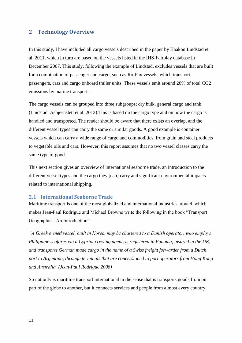
This next section gives an overview of international seaborne trade, an introduction to the
different vessel types and the cargo they [can] carry and significant environmental impacts
related to international shipping.
2.1 International Seaborne Trade Maritime transport is one of the most globalized and international industries around, which
makes Jean-Paul Rodrigue and Michael Browne write the following in the book “Transport
Geographies: An Introduction”:
“A Greek owned vessel, built in Korea, may be chartered to a Danish operator, who employs
Philippine seafares via a Cypriot crewing agent, is registered in Panama, insured in the UK,
and transports German made cargo in the name of a Swiss freight forwarder from a Dutch
port to Argentina, through terminals that are concessioned to port operators from Hong Kong
and Australia”(Jean-Paul Rodrigue 2008)
So not only is maritime transport international in the sense that is transports goods from on
part of the globe to another, but it connects services and people from almost every country.
12
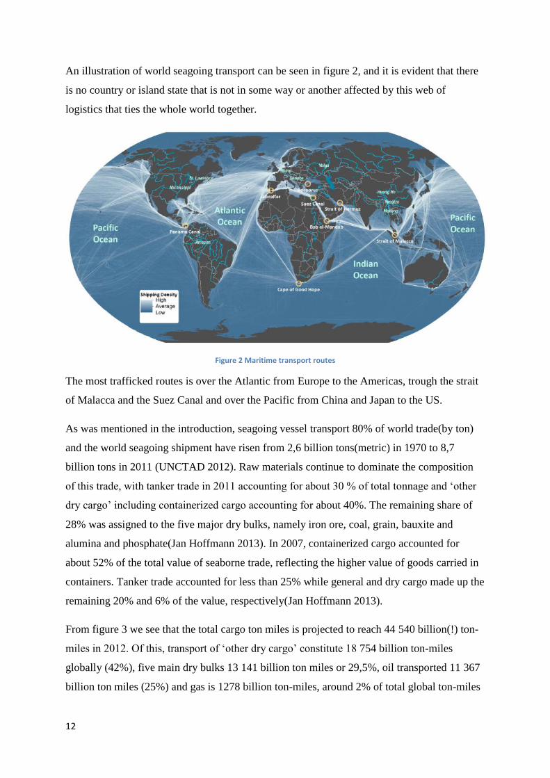
An illustration of world seagoing transport can be seen in figure 2, and it is evident that there
is no country or island state that is not in some way or another affected by this web of
logistics that ties the whole world together.
Figure 2 Maritime transport routes
The most trafficked routes is over the Atlantic from Europe to the Americas, trough the strait
of Malacca and the Suez Canal and over the Pacific from China and Japan to the US.
As was mentioned in the introduction, seagoing vessel transport 80% of world trade(by ton)
and the world seagoing shipment have risen from 2,6 billion tons(metric) in 1970 to 8,7
billion tons in 2011 (UNCTAD 2012). Raw materials continue to dominate the composition
of this trade, with tanker trade in 2011 accounting for about 30 % of total tonnage and ‘other
dry cargo’ including containerized cargo accounting for about 40%. The remaining share of
28% was assigned to the five major dry bulks, namely iron ore, coal, grain, bauxite and
alumina and phosphate(Jan Hoffmann 2013). In 2007, containerized cargo accounted for
about 52% of the total value of seaborne trade, reflecting the higher value of goods carried in
containers. Tanker trade accounted for less than 25% while general and dry cargo made up the
remaining 20% and 6% of the value, respectively(Jan Hoffmann 2013).
From figure 3 we see that the total cargo ton miles is projected to reach 44 540 billion(!) ton-
miles in 2012. Of this, transport of ‘other dry cargo’ constitute 18 754 billion ton-miles
globally (42%), five main dry bulks 13 141 billion ton miles or 29,5%, oil transported 11 367
billion ton miles (25%) and gas is 1278 billion ton-miles, around 2% of total global ton-miles
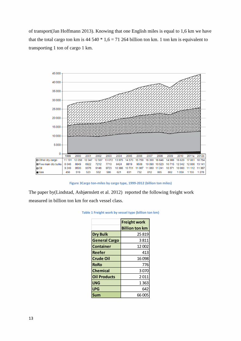
13
of transport(Jan Hoffmann 2013). Knowing that one English miles is equal to 1,6 km we have
that the total cargo ton km is 44 540 * 1,6 = 71 264 billion ton km. 1 ton km is equivalent to
transporting 1 ton of cargo 1 km.
Figure 3Cargo ton-miles by cargo type, 1999-2012 (billion ton miles)
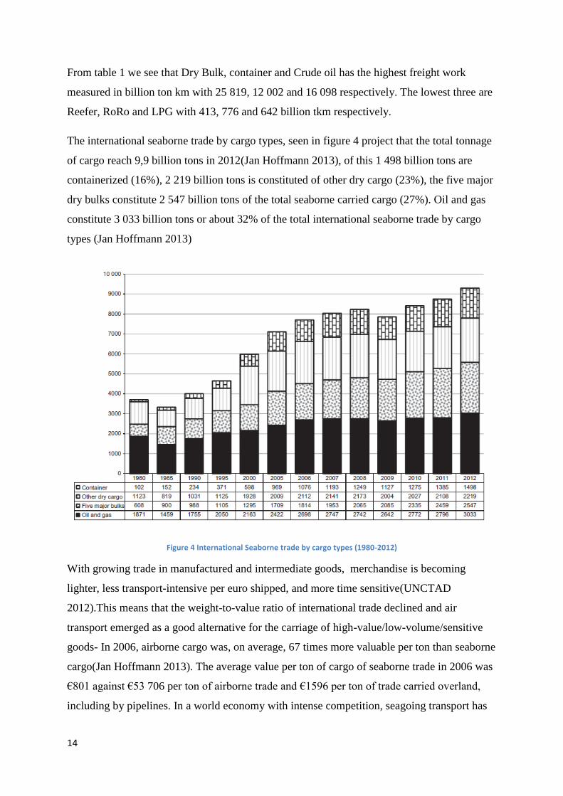
The paper by(Lindstad, Asbjørnslett et al. 2012) reported the following freight work
measured in billion ton km for each vessel class.
Table 1 Freight work by vessel type (billion ton km)
Freight work
Billion ton km
Dry Bulk 25 819
General Cargo 3 811
Container 12 002
Reefer 413
Crude Oil 16 098
RoRo 776
Chemical 3 070
Oil Products 2 011
LNG 1 363
LPG 642
Sum 66 005
14
From table 1 we see that Dry Bulk, container and Crude oil has the highest freight work
measured in billion ton km with 25 819, 12 002 and 16 098 respectively. The lowest three are
Reefer, RoRo and LPG with 413, 776 and 642 billion tkm respectively.
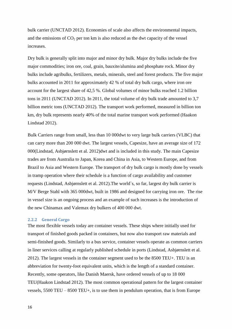
The international seaborne trade by cargo types, seen in figure 4 project that the total tonnage
of cargo reach 9,9 billion tons in 2012(Jan Hoffmann 2013), of this 1 498 billion tons are
containerized (16%), 2 219 billion tons is constituted of other dry cargo (23%), the five major
dry bulks constitute 2 547 billion tons of the total seaborne carried cargo (27%). Oil and gas
constitute 3 033 billion tons or about 32% of the total international seaborne trade by cargo
types (Jan Hoffmann 2013)
Figure 4 International Seaborne trade by cargo types (1980-2012)
With growing trade in manufactured and intermediate goods, merchandise is becoming
lighter, less transport-intensive per euro shipped, and more time sensitive(UNCTAD
2012).This means that the weight-to-value ratio of international trade declined and air
transport emerged as a good alternative for the carriage of high-value/low-volume/sensitive
goods- In 2006, airborne cargo was, on average, 67 times more valuable per ton than seaborne
cargo(Jan Hoffmann 2013). The average value per ton of cargo of seaborne trade in 2006 was
€801 against €53 706 per ton of airborne trade and €1596 per ton of trade carried overland,
including by pipelines. In a world economy with intense competition, seagoing transport has

15
the advantage of being relatively cheap, which will be demonstrated in section 4.1.2 in this
report, but it has the disadvantage of being more time consuming, especially compared to
airfreight.
2.2 World fleet structure and principal vessel types Following an annual growth of almost 10% the world fleet reached a total tonnage of 1 534
million dwt in early 2012. By the first quarter of the same year, there were 104 305 seagoing
commercial ships in service. Dry bulk carriers have the 40,6% of the total world capacity and
the world dry bulk fleet has surged by 60% in just four years. Oil tanker capacity accounts for
33,1 % of the world fleet while containerships make up 12,9% of the world tonnage
(UNCTAD 2012).
In January 2012 the average age of the fleet per dwt was 11,5 years, while on the other hand
the average age per vessel is twice that, at 21,9 years. This gives us an indication that older
vessels are much smaller and that newer vessel are comparably larger(UNCTAD 2012), 41,9
% of dry bulk tonnage is less than five years old, a very high share. The youngest fleet is that
of containerships with 64% under 10 years while the oldest is the general cargo and other
types of vessels.(UNCTAD 2012). Section 2.2.1 will give an overview of principal vessel
types while section 2.2.2 gives and introduction to fleet ownership. 2.3 describes significant
environmental impacts related to international shipping.
2.2.1 Dry Bulk
Bulk cargo is defines as loose cargo that is loaded directly into a ship`s hold. Bulk cargo is
thus a shipment such as oil, grain ores coal, cement, etc., or one which is not bundled, bottled,
or otherwise packed and which is loaded without counting or marking. A bulk carrier is
therefore a ship in which the cargo is carried in bulk, rather than in barrels, bags, containers,
etc., and is usually homogenous and capable of being loaded by gravity. Taking into
consideration the definition that is given above, there are two types of bulk carriers, dry bulk
carriers and wet-bulk carriers, the latter better known as tanker(Turbo 2012). Dry Bulk
carriers were developed in the 1950s to carry large quantities of non-packed commodities
such as grain, coal, iron ore, etc., in order to reduce transportation costs.
In order to remain competitive and maintain reasonable profit margins, distant suppliers such
as Brazilian iron ore producers see the use of large ships as a prerequisite to achieve
economies of scale. Transporting dry bulk in a relatively small Handymax vessel was, in
march 2012, three times as expensive per ton km than shipping the cargo in a large Capesize
16
bulk carrier (UNCTAD 2012). Economies of scale also affects the environmental impacts,
and the emissions of CO2 per ton km is also reduced as the dwt capacity of the vessel
increases.
Dry bulk is generally split into major and minor dry bulk. Major dry bulks include the five
major commodities; iron ore, coal, grain, bauxite/alumina and phosphate rock. Minor dry
bulks include agribulks, fertilizers, metals, minerals, steel and forest products. The five major
bulks accounted in 2011 for approximately 42 % of total dry bulk cargo, where iron ore
account for the largest share of 42,5 %. Global volumes of minor bulks reached 1.2 billion
tons in 2011 (UNCTAD 2012). In 2011, the total volume of dry bulk trade amounted to 3,7
billion metric tons (UNCTAD 2012). The transport work performed, measured in billion ton
km, dry bulk represents nearly 40% of the total marine transport work performed (Haakon
Lindstad 2012).
Bulk Carriers range from small, less than 10 000dwt to very large bulk carriers (VLBC) that
can carry more than 200 000 dwt. The largest vessels, Capesize, have an average size of 172
000(Lindstad, Asbjørnslett et al. 2012)dwt and is included in this study. The main Capesize
trades are from Australia to Japan, Korea and China in Asia, to Western Europe, and from
Brazil to Asia and Western Europe. The transport of dry bulk cargo is mostly done by vessels
in tramp operation where their schedule is a function of cargo availability and customer
requests (Lindstad, Asbjørnslett et al. 2012).The world`s, so far, largest dry bulk carrier is
M/V Berge Stahl with 365 000dwt, built in 1986 and designed for carrying iron ore. The rise
in vessel size is an ongoing process and an example of such increases is the introduction of
the new Chinamax and Valemax dry bulkers of 400 000 dwt.
2.2.2 General Cargo
The most flexible vessels today are container vessels. These ships where initially used for
transport of finished goods packed in containers, but now also transport raw materials and
semi-finished goods. Similarly to a bus service, container vessels operate as common carriers
in liner services calling at regularly published schedule in ports (Lindstad, Asbjørnslett et al.
2012). The largest vessels in the container segment used to be the 8500 TEU+. TEU is an
abbreviation for twenty-foot equivalent units, which is the length of a standard container.
Recently, some operators, like Danish Maersk, have ordered vessels of up to 18 000
TEU(Haakon Lindstad 2012). The most common operational pattern for the largest container
vessels, 5500 TEU – 8500 TEU+, is to use them in pendulum operation, that is from Europe

17
to Asia and back, Asia to North America and back, and from Europe to East Coast North
America. Total container trade volumes amounted to 151 million TEUs in 2011, equivalent to
about 1,4 billion tons.
General cargo is basically all cargo types which cannot be handled by grabs, conveyor belts,
pumps or pipeline system. This kind of cargo is then transported by general cargo vessels,
container vessels, reefer vessels and Ro-Ro vessels. Owners of specialized reefer tonnage
have suffered from the competition of containers that also cater for refrigerated containers.
Containers today account for about 60% of reefer cargo, and new container ships increasingly
include larger reefer capacities(UNCTAD 2012). General cargo vessels are typically used for
transport of pallets, bulk products in Big Bags, forest products, steel and aluminum, but also
containers (Lindstad, Asbjørnslett et al. 2012). Reefer vessels carry perishables such as food
and fresh fruit and frozen products while Ro-Ro vessels transport new and used cars, heavy
vehicles and project cargo(large, heavy, high value and/or critical pieces of equipment). Ro-
Ro vessels also transport trailer units with cargo.
2.2.3 Tank
Wet bulk cargoes typically consist of liquefied products and gas that are mainly transported in
wet bulk tankers, such as crude oil, liquefied petroleum gas(LPG) and liquefied natural gas
(LNG), or a family of similar products such as refined oil products by-product tankers and
chemical products by chemical tankers. Between 2000 and 2011, crude oil shipments grew
annually at an average rate than 1 %, a relatively slower pace than other market segments. In
2011 the total volume of crude oil loaded globally amounted to about 1.8 billion
tons(UNCTAD 2012). Tanker trade patterns are changing as crude oil source diversification
continues. A new map of crude supplies is being drawn up as new oil discoveries are made in
different regions and as new market suppliers emerge. As of now, western Asia remains the
largest loading area, followed by Africa, developing America and the transitioning
economies. The major importing economies are in ascending order Japan, North America,
Europe and developing Asia(UNCTAD 2012).
In 2011, world shipments of petroleum products and gas, including LNG and LPG) increased
by 5,1 %, a growth rate that reflects the booming LNG trade. The total shipment to 1,3 billion
tons. Natural gas is today the third largest source of energy after oil and coal(UNCTAD
2012).
18
2.2.4 Ship registration and Ship owning
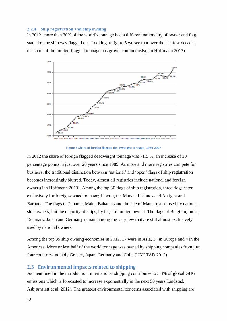
In 2012, more than 70% of the world`s tonnage had a different nationality of owner and flag
state, i.e. the ship was flagged out. Looking at figure 5 we see that over the last few decades,
the share of the foreign-flagged tonnage has grown continuously(Jan Hoffmann 2013).
Figure 5 Share of foreign flagged deadwheight tonnage, 1989-2007
In 2012 the share of foreign flagged deadweight tonnage was 71,5 %, an increase of 30
percentage points in just over 20 years since 1989. As more and more registries compete for
business, the traditional distinction between ‘national’ and ‘open’ flags of ship registration
becomes increasingly blurred. Today, almost all registries include national and foreign
owners(Jan Hoffmann 2013). Among the top 30 flags of ship registration, three flags cater
exclusively for foreign-owned tonnage; Liberia, the Marshall Islands and Antigua and
Barbuda. The flags of Panama, Malta, Bahamas and the Isle of Man are also used by national
ship owners, but the majority of ships, by far, are foreign owned. The flags of Belgium, India,
Denmark, Japan and Germany remain among the very few that are still almost exclusively
used by national owners.
Among the top 35 ship owning economies in 2012. 17 were in Asia, 14 in Europe and 4 in the
Americas. More or less half of the world tonnage was owned by shipping companies from just
four countries, notably Greece, Japan, Germany and China(UNCTAD 2012).
2.3 Environmental impacts related to shipping As mentioned in the introduction, international shipping contributes to 3,3% of global GHG
emissions which is forecasted to increase exponentially in the next 50 years(Lindstad,
Asbjørnslett et al. 2012). The greatest environmental concerns associated with shipping are
19
those relating to oil spills from accidents, equipment malfunctions or operational decisions.
There is even the concern that noise generated from ships can disturb the marine wildlife.
However, there are other core operational activities including loading and unloading and
associated service and support tasks than can have environmental and other impacts
(Shipbuilding 2010).
Apart from large oil spills and disasters like the Exxon Valdez, GWP related to maritime
logistics and the shipping sector have received very little attention relative to the impacts
from air and ground transport. Due to growing environmental concerns, on climate change in
particular, the attention towards environmental consequences from maritime transport are
likely to increase. Shipping is a major emitter of particulate matter(PM) and black
carbon(soot) and is also a large contributor of SO2 and NOx emissions. Soot from combusting
heavy fuel oils (HFOs) has a large content of black carbon. These dark particles, when
emitted into the atmosphere, absorb sunlight and is estimated to be the second largest
contributor to climate change after CO2(Shipbuilding 2010).It does not seem that there exists
a consensus on the actual emissions from the maritime transport sector. Its share of global
CO2 emissions ranges from 3% to 5%(Lindstad, Asbjørnslett et al. 2011),(IMO 2009),(Vidal
2008) while the sector is estimated to account for 4%-8% of SO2 emissions and about 15% of
Nox emissions(Tzannatos 2010).
Having this in mind, one can summarize the primary environmental challenges in maritime
logistics to atmospheric emissions due to the combustion of HFO and impacts from spills of
substances like oil, cargo residues, anti-fouling paint and ballast water (Shipbuilding 2010).
Fuel cost can amount up to 40% of a ship`s total operating costs. Large freight ships, like the
ones described in this report all run on a particular form of diesel known as bunker fuel or
heavy fuel oil. The fuel can only be described as a black mud of hydrocarbons. It is a very
dense and highly polluting residual substance from the oil refining process, and the world
fleet consume millions upon millions of tons of it every year. Due to the fact that it bunker
fuel is a residual substance, it carries everything that does not distil during the oil refining
process, including a large number of pollutants. (Shipbuilding 2010). There are ways to
remove the number of pollutants in the bunker fuel, but they are not economically attractive.
As the residual character of bunker fuel keeps the price low, it does not give any incentives to
the shipowners to switch to cleaner fuels(Shipbuilding 2010). They only see an incentive of
reducing the bunker fuel use per ton km to reduce costs in an increasingly competitive market,
20
often by building bigger ships and thus achieving economies of scale(Lindstad, Asbjørnslett et
al. 2012) or in some cases reducing the speed. Even though they are in early stages, and some
are more viable than others, there exists today several alternatives to bunker fuels or ways to
reduce the use of it. A few examples are increased use of biodiesel, wind and solar power,
LNG, and air lubrication. This without mentioning how innovative ship design can help
reduce fuel use, drag and fuel composition(Shipbuilding 2010).

21
3 Methodology This chapter aims at giving the reader some insight in the methodologies used to improve the
EXIOBASE dataset and calculating the GWP of international maritime transport. The first
section explain the fundamental theory of Life Cycle Assessment, its goal, how Life Cycle
Inventories(LCI`s) are built and how environmental impacts are assessed. The second section
gives and overview of Environmentally Extended Multiregional Input-Output (EE MRIO), the
EXIOBASE dataset and how Emissions Embodied in Trade(EET) are calculated.
3.1 Life Cycle Assessment
3.1.1 What is LCA?
According to the book “Methodological essentials of Life Cycle Assessment” by Anders
Hammer Strømman, the objective of a LCA is to
“..Perform consistent comparisons of technological systems with respect to their
environmental impacts”
LCA incorporates the entire life cycle of a product, from material extraction, production,
transport, use and waste which allows us to quantify and analyze the true total environmental
impact of a product. It is important to note that a LCA is not necessarily including all of the
life cycles phases from cradle to grave. Some studies only include certain life cycle stages,
like production and use, but leave out for example end-of-live management. LCA also allows
us to deal with the issue of problem shifting (Strømman 2010). Problem shifting is when one,
by solving one type of environmental problem, creates or enhances another in the process. For
example, if one wish to reduce the greenhouse gas emissions from a crop by reducing the use
of artificial fertilizer you might increase the impact on land-use due to the fact that more land
area is needed to grow the same amount of output from the crop as you did using fertilizer.
To summarize, LCA is a methodology for the evaluation of potential environmental impacts
from a given product system, taking the whole life cycle of the product into account. The
common purpose of LCA is to quantify and document the potential environmental impacts as
a basis for focus on how to make improvements so to reduce the environmental impact of the
product or service, to compare alternative product designs, identify beneficial waste
management solutions and get a good basis for external communication or development of
policies and actions.
An LCA has four phases:
22
1. Goal and scope definition
2. Life cycle inventory(LCI)
3. Life cycle impact assessment(LCIA)
4. Interpretation
3.1.2 Goal and Scope
The goal and scope definition starts with defining the problem formulation and system
definition, what are the objectives of the LCA and what the decision context of the study is. It
also defines the functional unit of the LCA, the system boundaries and data collection
strategies. The functional unit defines the function that the product system provides to the
users. It is a reference to which inputs and outputs are related, in the way one can determine
the reference flows in the product system in order to fulfill the intended functions. The
functional unit also specifies in which quantity, for what duration, to what quality, and it also
considers changes in the functional performance over time. A functional unit can for example,
in the context of maritime transport, be “1 ton km”. In this case, an LCA will find the
potential environmental impacts of the given vessel per km one ton of cargo are transported.
3.1.3 Life cycle Inventory(LCI)
The LCI phase quantifies the sum of all elementary flows (inputs from and outputs back to
nature) of the product system, according to the chosen functional unit. The LCI is regarded as
the most time consuming phase of a LCA. Some data are often available in databases but most
commonly the person or group that is performing the LCA need to collect the data required
for the special case of the study.
To perform an LCA two types of data are distinguished:
1. Foreground data
2. Background data
There is no sharp distinction between foreground and background data, but generally the
foreground data is defined as the system you model and investigate in detail such as direct
emissions and use of raw materials. The background data is generic data from existing
databases that you use to complete value chains upstream in the process, such as emissions
related to the production of raw materials and energy(Strømman 2010).
3.1.4 Impact Categories
When assessing the environmental impacts of maritime transport this report analyze the
Global Warming Potential(GWP). This method, applied in Life Cycle Impact Assessment
23
(LCIA), convert the emissions of hazardous substances and extractions of natural resources
into impact categories which are divided into to levels(Mark Goedkoop 2009). The LCIA
phase aims to determine the potential environmental impacts caused by the elementary flows
from the LCI by using midpoint or endpoint impact category indicators. On midpoint level, a
higher number of impact categories is differentiated and the results are more accurate and
precise compared to the three areas of protection at endpoint level (Brattebø 2011).
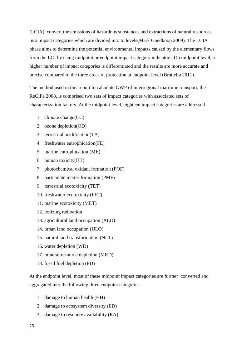
The method used in this report to calculate GWP of interregional maritime transport, the
ReCiPe 2008, is comprised two sets of impact categories with associated sets of
characterization factors. At the midpoint level, eighteen impact categories are addressed.
1. climate change(CC)
2. ozone depletion(OD)
3. terrestrial acidification(TA)
4. freshwater eutrophication(FE)
5. marine eutrophication (ME)
6. human toxicity(HT)
7. photochemical oxidant formation (POF)
8. particulate matter formation (PMF)
9. terrestrial ecotoxicity (TET)
10. freshwater ecotoxicity (FET)
11. marine ecotoxicity (MET)
12. ionizing radioation
13. agricultural land occupation (ALO)
14. urban land occupation (ULO)
15. natural land transformation (NLT)
16. water depletion (WD)
17. mineral resource depletion (MRD)
18. fossil fuel depletion (FD)
At the endpoint level, most of these midpoint impact categories are further converted and
aggregated into the following three endpoint categories:
1. damage to human health (HH)
2. damage to ecosystem diversity (ED)
3. damage to resource availability (RA)
24
(Mark Goedkoop 2009)
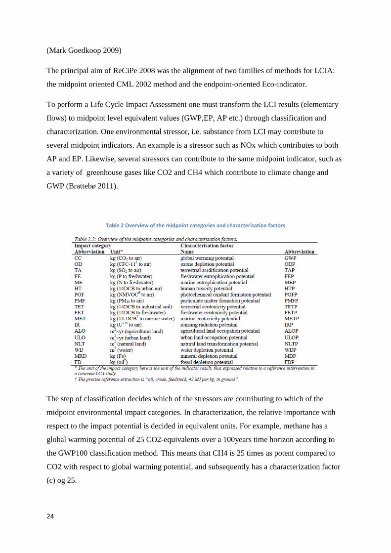
The principal aim of ReCiPe 2008 was the alignment of two families of methods for LCIA:
the midpoint oriented CML 2002 method and the endpoint-oriented Eco-indicator.
To perform a Life Cycle Impact Assessment one must transform the LCI results (elementary
flows) to midpoint level equivalent values (GWP,EP, AP etc.) through classification and
characterization. One environmental stressor, i.e. substance from LCI may contribute to
several midpoint indicators. An example is a stressor such as NOx which contributes to both
AP and EP. Likewise, several stressors can contribute to the same midpoint indicator, such as
a variety of greenhouse gases like CO2 and CH4 which contribute to climate change and
GWP (Brattebø 2011).
Table 2 Overview of the midpoint categories and characterisation factors
The step of classification decides which of the stressors are contributing to which of the
midpoint environmental impact categories. In characterization, the relative importance with
respect to the impact potential is decided in equivalent units. For example, methane has a
global warming potential of 25 CO2-equivalents over a 100years time horizon according to
the GWP100 classification method. This means that CH4 is 25 times as potent compared to
CO2 with respect to global warming potential, and subsequently has a characterization factor
(c) og 25.
25
3.2 EEIO-MRIO The application of multi-regional input-output(MRIO) modeling to environmental flows is a
useful methodology to evaluate global linkages between consumption and production
systems. MRIO studies can assess environmental impacts from individual products,
household consumption, transport, and international climate policy(Glen Peters 2009).
Traditional input-output focus on the inter-industry requirements of a single economy, nation
or region, i.e., what the different sectors of industry require from each other to produce one
unit of output for each industry. MRIO models on the other hand takes it a step further and
includes total inter-industry requirements both within and between different world regions to
produce one unit of output for each industry, i.e. a MRIO model includes imports and exports.
International trade provides an mechanism to geographically separate consumption and the
environmental impacts in production. Through international trade, polluting and low value-
added production can be relocated to distant lands, while the domestic economy increases
high value-added and cleaner production(Peters 2007). An environmentally-extended MRIO
model makes it possible to not only assess the division between low and big value-added
production between regions, but also to assess the environmental impacts of the inter-industry
requirements between regions. The model also make it possible to go into more detail on
specific trade flows, like assessing the trade flows and environmental impacts of seagoing
transport necessary to accommodate the inter-industry requirements between regions
In this study EE MRIO is used as an extension of hybrid-LCA to consider regional trade and
global emissions. Typically, LCA is focused on individual products or processes, but the
production system may still be global.
There are several practical issues that need to be considered when a EE MRIO analysis is
performed. According to the paper “The application of Multi-Regional Input-Output analysis
to Industrial Ecology” by Glen Peters and Edgar Hertwich one of the greatest challenges to
perform a detailed MRIO study is the general data availability. IO data from more or less
every country is required, which is generally available for most OECD countries, but for
relatively few non-OECD countries. On top of that, regions like OECD Europe and North
America submit data using different classifications and formats. There exists several data
projects that have built large IO databases for global models such as GTAP(the Global Trade,
Assistance, and Production project) and EXIOBASE which is used in this report. GTAP
provides data for 87 world regions in 57 sector detail(Glen Peters 2009) while EXIOBASE

26
provides data for 9 regions in 138 sector detail. Already advantages and disadvantages
between the models are evident. The GTAP models has a higher resolution on regions but
fewer and more aggregated sectors while EXIOBASE have a better resolution on sectors but
fewer regions.
Other practical issues regarding MRIO modeling include exchange rates, inflation, and sector
aggregation (Glen Peters 2009).
3.2.1 EXIOBASE
To analyze the flows that is transported with seagoing vessels and their environmental
impacts, the Input-Output database EXIOBASE will be used. EXIOBASE is a global, multi-
regional Environmentally-extended Input-Output (EEIO) table and is result of the EXIOPOL
project. EXIOPOL was a EU-funded project that had two main goals. One part of the project
aimed at improving insights in external costs of environmental pressures, the other part tried
to overcome significant limitations in existing data sources in the field of multiregional
environmentally extended Supply and Use tables (MR EE SUTs), that is to produce the
EXIOBASE(Richard Wood 2013). Statistical Institutes provide SUT and IOT for single
countries, without trade links. Sector and product detail is not as good as it ought to be.
Environmental extensions are often lacking or include only a few types of emissions and
primary resource uses. Also, there is little or no harmonization of sector and product
classification across different countries. It is therefore difficult to assess the extent to which a
country induces environmental impacts abroad via trade, or in the case of this report, assess
the environmental impacts due to maritime transport of products and goods between regions.
The MR EE I-O database, i.e EXIOBASE, that is developed in EXIOPOL aims to make
crucial advances in quality. The EXIOPOL project´s aim is really to leapfrog: it gives EU a
fully fledged, detailed, transparent, public global MR EE I-O database with externalities,
allowing for numerous types of analyses for policy support purposes(Richard Wood 2013).
This database covers the entire global economy, which is grouped into 9 regions:
1. India
2. China
3. OECD Europe
4. OECD North America
5. OECD Pacific
6. Other Developing Asia
27
7. Economies in transition
8. Latin America
9. Africa and Middle East
The database show the complex trade between regions and is ideal to analyze the
environmental impacts of maritime logistics due to the trade between regions.
The EXIOBASE dataset is a Supply and Use Table (SUT) that has been converted to a 138 x
138 product Symmetric Input Output Table (SIOT). The product SIOT was selected over the
industry SIOT because ships transport products and commodities, not industries. This being
said, both the product and industry classification names are the same, and it is often more
convenient to think of these “products from an industry” as “industries” themselves.
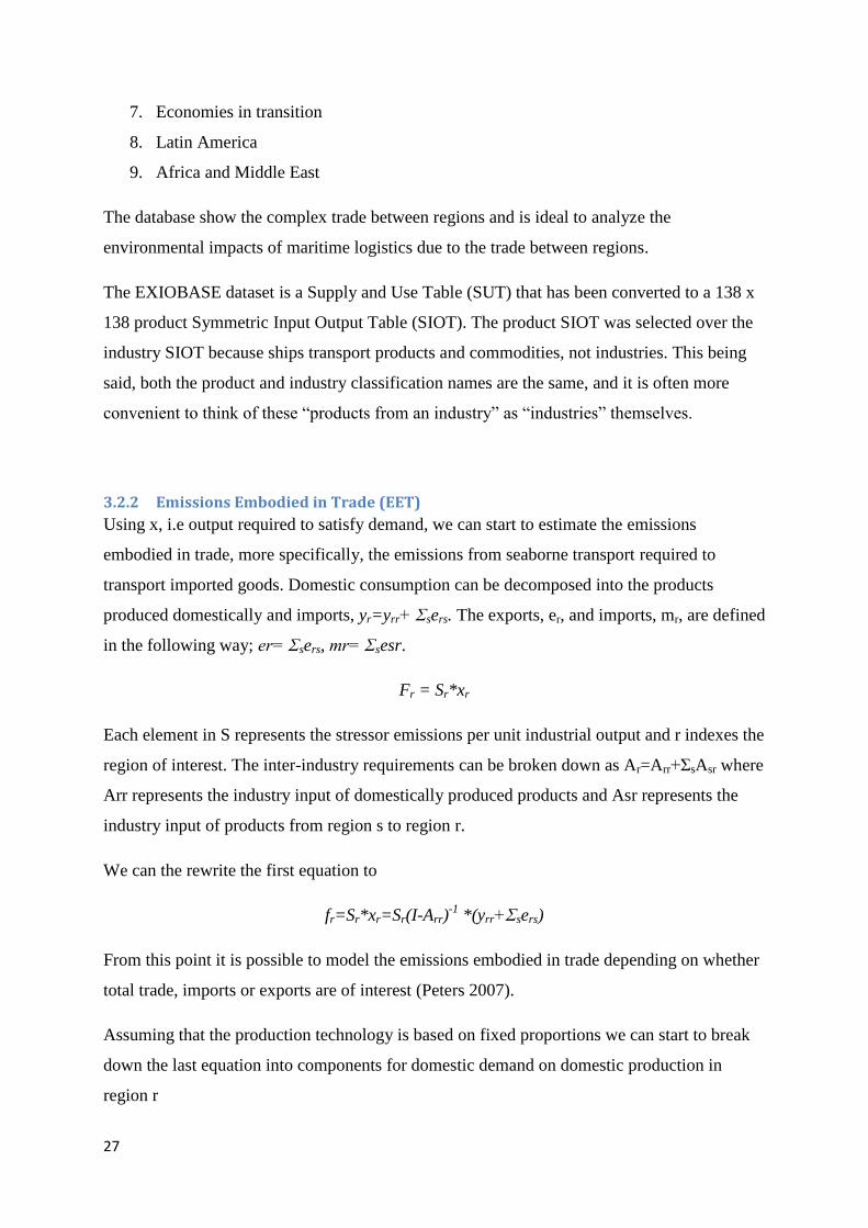
3.2.2 Emissions Embodied in Trade (EET)
Using x, i.e output required to satisfy demand, we can start to estimate the emissions
embodied in trade, more specifically, the emissions from seaborne transport required to
transport imported goods. Domestic consumption can be decomposed into the products
produced domestically and imports, yr=yrr+ Ʃsers. The exports, er, and imports, mr, are defined
in the following way; er= Ʃsers, mr= Ʃsesr.
Fr = Sr*xr
Each element in S represents the stressor emissions per unit industrial output and r indexes the
region of interest. The inter-industry requirements can be broken down as Ar=Arr+ƩsAsr where
Arr represents the industry input of domestically produced products and Asr represents the
industry input of products from region s to region r.
We can the rewrite the first equation to
fr=Sr*xr=Sr(I-Arr)-1
*(yrr+Ʃsers)
From this point it is possible to model the emissions embodied in trade depending on whether
total trade, imports or exports are of interest (Peters 2007).
Assuming that the production technology is based on fixed proportions we can start to break
down the last equation into components for domestic demand on domestic production in
region r

28
frr=Sr(I-Arr)-1
*yrr
And the EET from region r to region s
Frs = Sr(I-Arr)-1
* Ʃsers
Adding these gives the total emissions occuring in the country
fr = frr+Ʃsfrs
The total Emissions Embodied in Imports(EEI) is obtained by the following summation;
Fmr = Ʃsfsr

29
4 System Description This chapter aims at clarifying all assumptions, calculations and technical specification used
in this report. The first section focus on maritime transport and how the Inventory of each ship
is constructed. The second section focus on how the EXIOBASE data set is improved by
describing the assumption made and the approach that is taken to calculate the seagoing trade
between the regions and the associated environmental impact.
4.1 Maritime Transportation
As mentioned in the introduction, this report use ships found in the study (Lindstad,
Asbjørnslett et al. 2012) and (Lindstad, Asbjørnslett et al. 2011). The vessel differ quite
considerably in size between classes but the size difference between vessels of the same class
can also be large. Smaller vessels, those between 0 – 15000 dwt typically operate in short sea
trades or coastal shipping trades while larger vessels operate on the transcontinental trades.
The size of the vessels used in this report are close to the average sized vessel of each class,
this to be able to model both short and long distance transport.
The ship classes used in this report are the main cargo carrying vessels on the oceans today
are the following:
Large Dry bulk
Dry bulk
General Cargo
Container
Reefer
Crude Oil
RoRo
Chemicals
Oil Products
LNG
LPG
The following section will go through the assumptions, requirements and calculation steps
made to improve the EXIOBASE dataset and calculate Global Warming Potential(GWP) of
international seagoing transport.

30
4.1.1 Flowchart of vessels
Figure 6 Generic vessel flowchart
Figure 6 shows a simplified flowchart of they key inputs into a seagoing transport vessel.
Steel is used to construct the hull, copper to construct the propeller and heavy fuel oil (HFO)
is the propulsion energy source. To be able to assess the environmental impacts of 1tkm of
transport, a life cycle inventory(LCI) of each vessel has to to be constructed. Constructing a
LCI is a detail oriented and time consuming process, and to be able to build LCIs of 11 ships
within the time scope of this thesis some assumptions on key material and energy inputs had
to made. These assumptions where made in dialogue with my supervisor Anders H.
Strømman and co-supervisor Haakon Lindstad. The decision was made to focus on three key
inputs
Steel
Copper
Fuel
Steel is, the largest input of a single material in the construction of any vessel as a ship is
basically a floating steel structure. Steel production is an energy intensive activity and is
responsible for large part of environmental impacts when constructing a ship. A lot of effort
has therefore been put on finding accurate numbers of steel use per vessel. Copper is an
interesting material to look at, especially since it is rather expensive and thus can have a
significant effect on the € input per € of transport. The refining of copper is also quite energy
intensive and responsible for considerable emissions of greenhouse gasses. Copper is assumed
to be the main input of the construction of the propeller. Fuel consumption is arguably the
most import important input and is contribute considerably to both cost and emissions of
31
seagoing transport. Heavy Fuel Oil(HFO) is assumed to be the fuel of choice to power the
ships described in this thesis and it is discussed in more detail in the section 2.3. Consumption
of HFO varies between the ship classes and is a key component in assessing the cost and
emission differences between them.
4.1.2 Technical vessel data
The following section introduces the input data and calculation methods used to derive key
numbers like steel, copper and fuel consumption.
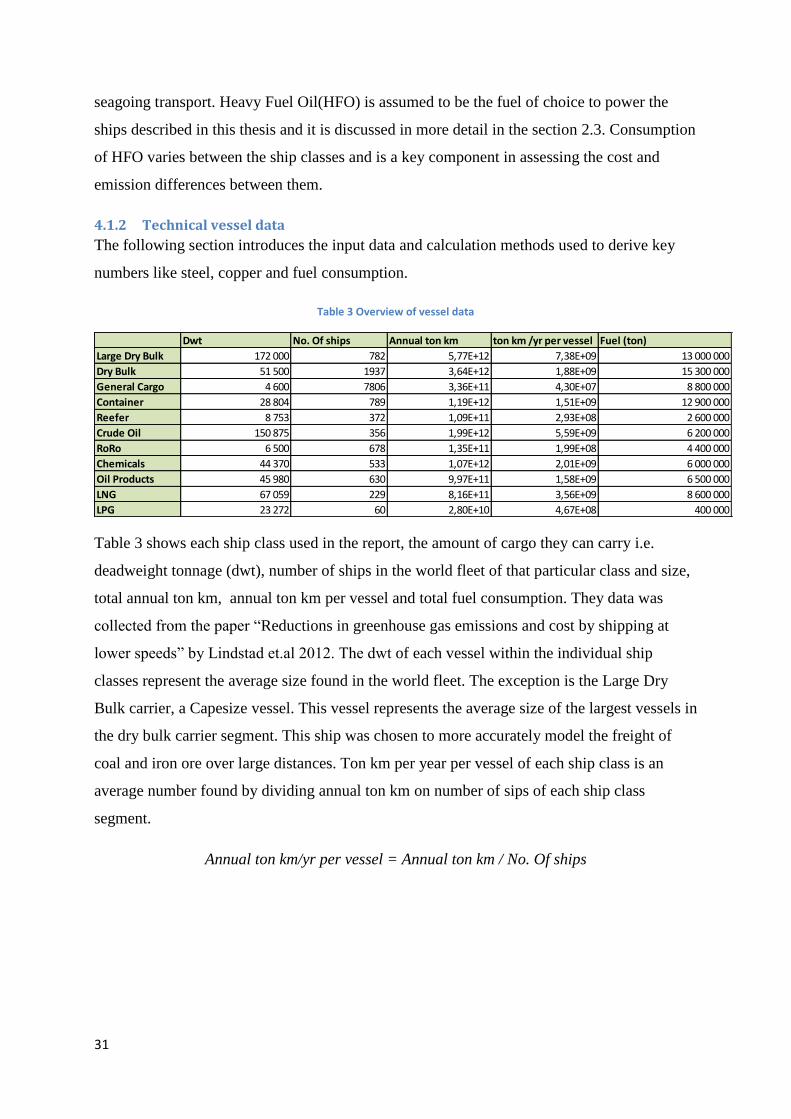
Table 3 Overview of vessel data
Table 3 shows each ship class used in the report, the amount of cargo they can carry i.e.
deadweight tonnage (dwt), number of ships in the world fleet of that particular class and size,
total annual ton km, annual ton km per vessel and total fuel consumption. They data was
collected from the paper “Reductions in greenhouse gas emissions and cost by shipping at
lower speeds” by Lindstad et.al 2012. The dwt of each vessel within the individual ship
classes represent the average size found in the world fleet. The exception is the Large Dry
Bulk carrier, a Capesize vessel. This vessel represents the average size of the largest vessels in
the dry bulk carrier segment. This ship was chosen to more accurately model the freight of
coal and iron ore over large distances. Ton km per year per vessel of each ship class is an
average number found by dividing annual ton km on number of sips of each ship class
segment.
Annual ton km/yr per vessel = Annual ton km / No. Of ships
Dwt No. Of ships Annual ton km ton km /yr per vessel Fuel (ton)
Large Dry Bulk 172 000 782 5,77E+12 7,38E+09 13 000 000
Dry Bulk 51 500 1937 3,64E+12 1,88E+09 15 300 000
General Cargo 4 600 7806 3,36E+11 4,30E+07 8 800 000
Container 28 804 789 1,19E+12 1,51E+09 12 900 000
Reefer 8 753 372 1,09E+11 2,93E+08 2 600 000
Crude Oil 150 875 356 1,99E+12 5,59E+09 6 200 000
RoRo 6 500 678 1,35E+11 1,99E+08 4 400 000
Chemicals 44 370 533 1,07E+12 2,01E+09 6 000 000
Oil Products 45 980 630 9,97E+11 1,58E+09 6 500 000
LNG 67 059 229 8,16E+11 3,56E+09 8 600 000
LPG 23 272 60 2,80E+10 4,67E+08 400 000
32
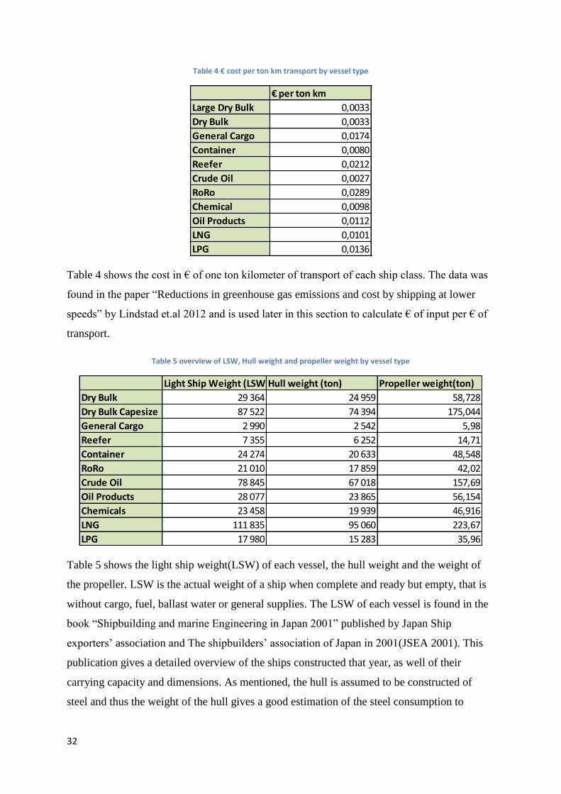
Table 4 € cost per ton km transport by vessel type
Table 4 shows the cost in € of one ton kilometer of transport of each ship class. The data was
found in the paper “Reductions in greenhouse gas emissions and cost by shipping at lower
speeds” by Lindstad et.al 2012 and is used later in this section to calculate € of input per € of
transport.
Table 5 overview of LSW, Hull weight and propeller weight by vessel type
Table 5 shows the light ship weight(LSW) of each vessel, the hull weight and the weight of
the propeller. LSW is the actual weight of a ship when complete and ready but empty, that is
without cargo, fuel, ballast water or general supplies. The LSW of each vessel is found in the
book “Shipbuilding and marine Engineering in Japan 2001” published by Japan Ship
exporters’ association and The shipbuilders’ association of Japan in 2001(JSEA 2001). This
publication gives a detailed overview of the ships constructed that year, as well of their
carrying capacity and dimensions. As mentioned, the hull is assumed to be constructed of
steel and thus the weight of the hull gives a good estimation of the steel consumption to
€ per ton km
Large Dry Bulk 0,0033
Dry Bulk 0,0033
General Cargo 0,0174
Container 0,0080
Reefer 0,0212
Crude Oil 0,0027
RoRo 0,0289
Chemical 0,0098
Oil Products 0,0112
LNG 0,0101
LPG 0,0136
Light Ship Weight (LSW)Hull weight (ton) Propeller weight(ton)
Dry Bulk 29 364 24 959 58,728
Dry Bulk Capesize 87 522 74 394 175,044
General Cargo 2 990 2 542 5,98
Reefer 7 355 6 252 14,71
Container 24 274 20 633 48,548
RoRo 21 010 17 859 42,02
Crude Oil 78 845 67 018 157,69
Oil Products 28 077 23 865 56,154
Chemicals 23 458 19 939 46,916
LNG 111 835 95 060 223,67
LPG 17 980 15 283 35,96

33
construct each ship. Both the weight of the hull and propeller, an thus the assumed
consumption of steel and copper, is calculated as a fraction of the light ship weight. The basis
of the fraction used is found in the report “LCA-ship”(Karl Jivén 2004), which documents the
assumptions made in a life cycle analysis program for ships. The hull weight is be estimated
to be 85% of the light ship weight while the propeller weight is assumed to be 0,2% of the
light ship weight.
Hull weight = LSW*0,85
Propeller weight = LSW*0,002
Table 6 Material requirements per vessel type
Table 6 gives the total steel and copper consumption per vessel and the average fuel
consumption per tkm for each ship class. The steel and copper use were calculated in the way
described in the previous paragraph. The fuel consumption per tkm was calculated by
dividing the total annual fuel consumption per ship class on the total annual ton km of the
same ship class. Annual fuel consumption and total annual ton km is found in table 3
fuel(ton) per ton km = Fuel(ton)/annual ton km
Step 1 Steel (ton) Copper (ton) fuel per ton km(ton)
Large Dry Bulk 7,44E+04 1,75E+02 2,25E-06
Dry Bulk 2,50E+04 5,87E+01 4,20E-06
General Cargo 2,54E+03 5,98E+00 2,62E-05
Container 6,25E+03 1,47E+01 1,08E-05
Reefer 2,06E+04 4,85E+01 2,39E-05
Crude Oil 1,79E+04 4,20E+01 3,12E-06
RoRo 6,70E+04 1,58E+02 3,26E-05
Chemical 2,39E+04 5,62E+01 5,61E-06
Oil Products 1,99E+04 4,69E+01 6,52E-06
LNG 9,51E+04 2,24E+02 1,05E-05
LPG 1,53E+04 3,60E+01 1,43E-05

34
Table 7 Material requirements per ton km by vessel type
Table 7 show the consumption of steel, copper and fuel per ton km. The fuel data on fuel
consumption are the same numbers as shown in table 6 while the steel and copper use per ton
km are calculated using data on lifetime and average annual ton km data per vessel.
The lifetime of each vessel is assumed to be 25 years(Lindstad, Asbjørnslett et al. 2012) and
the average annual ton km per vessel is found in table 3.
Steel(ton) per ton km = Steel(ton)*1/(ton km/yr vessel*lifetime)
Table 8 € cost of material requirements per ton km by vessel type
Table 9 € cost per ton material
Step 2 Steel (ton) per ton km Copper (ton) per ton km fuel(ton) per ton km
Large Dry Bulk 4,03E-07 9,49E-10 2,25E-06
Dry Bulk 5,31E-07 1,25E-09 4,20E-06
General Cargo 2,36E-06 5,56E-09 2,62E-05
Container 1,65E-07 3,89E-10 1,08E-05
Reefer 2,82E-06 6,63E-09 2,39E-05
Crude Oil 1,28E-07 3,01E-10 3,12E-06
RoRo 1,35E-05 3,17E-08 3,26E-05
Chemical 4,76E-07 1,12E-09 5,61E-06
Oil Products 5,04E-07 1,19E-09 6,52E-06
LNG 1,07E-06 2,51E-09 1,05E-05
LPG 1,31E-06 3,08E-09 1,43E-05
Step 3 € Steel per ton km € Copper per ton km € fuel per ton km
Large Dry Bulk 2,28E-04 5,99E-06 1,23E-03
Dry Bulk 3,01E-04 7,88E-06 2,29E-03
General Cargo 1,34E-03 3,51E-05 1,43E-02
Container 9,37E-05 2,46E-06 5,90E-03
Reefer 1,60E-03 4,18E-05 1,30E-02
Crude Oil 7,24E-05 1,90E-06 1,70E-03
RoRo 7,62E-03 2,00E-04 1,78E-02
Chemical 2,69E-04 7,06E-06 3,06E-03
Oil Products 2,85E-04 7,48E-06 3,56E-03
LNG 6,04E-04 1,58E-05 5,75E-03
LPG 7,42E-04 1,94E-05 7,80E-03
Product Price per ton (€)
HFO 546,00
Copper 6 310,20
Steel 566,28

35
Table 8 shows the value in € of the amount of steel, copper and fuel consumed pr ton km. The
data is found by multiplying the € value of 1ton of the product, table 9, with steel, copper and
fuel consumption per ton km
Table 10 € cost of material per € transport by vessel type
Table 10 shows the € value of steel, fuel and copper per € of transport. These numbers are
found by dividing the € value of steel, copper and fuel on the general cost per ton tkm of each
vessel class found in table 4. This data shows the final input numbers which will be
incorporated into the Hybrid-MRIO model which will be discussed in more detail in the next
section. In short these number gives the € of input of steel, copper and fuel per € euro
transport i.e. output. Through the calculations shown is this section, technical vessel data has
been transformed from total requirements of steel, copper and fuel per vessel into input
coefficients necessary to complete the model.
Step 4 € Steel per € transport € Copper per € transport € fuel per € transport
Large Dry Bulk 6,95E-02 1,82E-03 3,74E-01
Dry Bulk 9,15E-02 2,40E-03 6,98E-01
General Cargo 7,71E-02 2,02E-03 8,24E-01
Container 1,17E-02 3,07E-04 7,37E-01
Reefer 7,54E-02 1,98E-03 6,15E-01
Crude Oil 2,67E-02 7,00E-04 6,27E-01
RoRo 2,63E-01 6,91E-03 6,15E-01
Chemical 2,76E-02 7,24E-04 3,14E-01
Oil Products 2,56E-02 6,70E-04 3,19E-01
LNG 6,00E-02 1,57E-03 5,71E-01
LPG 5,45E-02 1,43E-03 5,73E-01
36
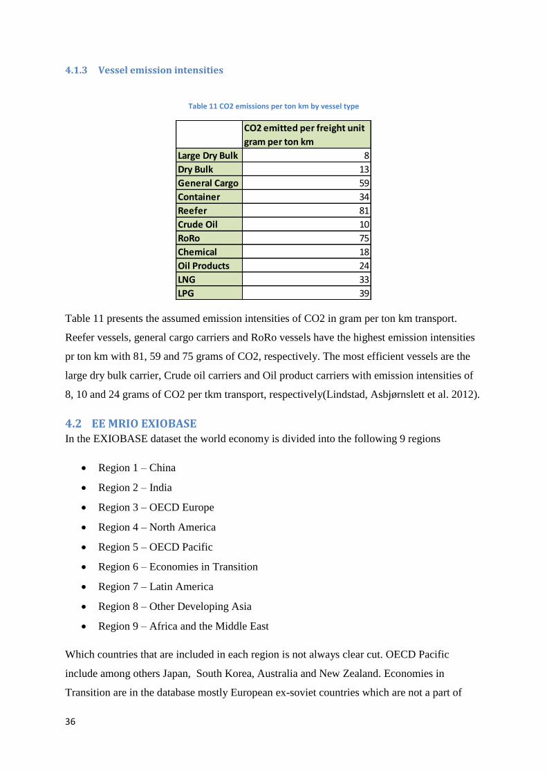
4.1.3 Vessel emission intensities
Table 11 CO2 emissions per ton km by vessel type
Table 11 presents the assumed emission intensities of CO2 in gram per ton km transport.
Reefer vessels, general cargo carriers and RoRo vessels have the highest emission intensities
pr ton km with 81, 59 and 75 grams of CO2, respectively. The most efficient vessels are the
large dry bulk carrier, Crude oil carriers and Oil product carriers with emission intensities of
8, 10 and 24 grams of CO2 per tkm transport, respectively(Lindstad, Asbjørnslett et al. 2012).
4.2 EE MRIO EXIOBASE In the EXIOBASE dataset the world economy is divided into the following 9 regions
Region 1 – China
Region 2 – India
Region 3 – OECD Europe
Region 4 – North America
Region 5 – OECD Pacific
Region 6 – Economies in Transition
Region 7 – Latin America
Region 8 – Other Developing Asia
Region 9 – Africa and the Middle East
Which countries that are included in each region is not always clear cut. OECD Pacific
include among others Japan, South Korea, Australia and New Zealand. Economies in
Transition are in the database mostly European ex-soviet countries which are not a part of
CO2 emitted per freight unit
gram per ton km
Large Dry Bulk 8
Dry Bulk 13
General Cargo 59
Container 34
Reefer 81
Crude Oil 10
RoRo 75
Chemical 18
Oil Products 24
LNG 33
LPG 39

37
OECD Europe like Russia, Slovenia, Bulgaria and Latvia, but the region also include Cyprus
and Malta. Other Developing Asia include, to mention a few, Taiwan and Indonesia.
The regions are organized into a 9by9 matrix.
Figure 7 EXIOBASE 9 region structure
Each region and its trade flows are given by individual A-matrices. An A-matrix, also called
coefficient matrix or requirements matrix, gives us € of input required per € of output. It show
what each region require from itself, i.e. its own sectors, from the other 8 regions and what it
export to the other regions.
Figure 8 Domestic requirements

38
Figure 9 Import requirements
Figure 10 Export requirements
To understand the dynamics of this model take a look on the three figures shown above.
Figure 8 shows the domestic requirements of region 1 i.e. what the domestic sectors require
from each other in order to produce 1€ of output. Figure 9 show the import requirements of
region 1 from the other 8 regions, i.e. what the domestic sectors require from foreign sectors
to produce one unit output. Figure 10 shows the export requirements from region 1 to the
other regions i.e. what the other 8 regions require from region 1 to produce 1 € of output. The
rule is that the domestic requirements of each region is found on the diagonal of 9by9 region
model, the import requirements are found on the vertical axis while the regions export are
found on the horizontal axis.

39
4.2.1 The A-matrix
Each one of these individual A-matrices shown i figure 11 are structure in one of two ways
Figure 11 Modified Arr matrix
This figure show us in more detail how each on of the individual domestic A-matrices on the
diagonal is constructed. The Ar,r is build up by 138x138 sectors whose values are given by
€/€. The logic is the same as in the big region matrix shown on the previous page. For a given
output of 1€ a sector requires fractions of € from the other sectors. To simplify, one can think
of it as a recipe; to produce 1€ worth of paddy rice, you need x€ worth of road transportation,
y€ worth of fertilizer and z€ worth of iron ore. The horizontal axis shows what each sector
gives to itself and the other 137 sectors while the vertical axis shows what each sector
requires from itself and the other 137 sectors to produce 1€ worth of product. The Ar,r matrix
represents the diagonal region matrices, i.e. what each region requires from itself. This figure
also cuts to the core of this thesis, where one of the main tasks is to improve the
representation of maritime transport. The EXIOBASE dataset has one sector, sea and coastal
water transportation services, that cover all maritime trade between regions. That means that
all goods, iron ore, minerals, crude oil, wheat and electronics are transported in the same boat.
The matrix on the right of figure 12, Atr_€/tkm is the improvement of this model. It is a 138
by 11 matrix that shows the requirements in € of each of the 11 vessels from the 138 sectors
to transport one ton of goods one kilometer. In short, the matrix is constructed by creating an
average “sea and coastal water transportation services”-vector, figure 12, from all the 9
regions and then substituting the €/€ inputs of steel, fuel and copper with the values from the
life cycle inventories of the individual ship classes shown in table 10 in 4.1.2. The next step is

40
to convert Atr_€/€ into an Atr_€/tkm matrix by multiplying with the general € cost per ton km
of each vessel, shown i table 4.
Figure 12 Modified Atr €/€ matrix
The first step to construct Atr_€/tkm matrix is to insert the €/€ values calculated in table 10
for each of the 11 ship classes into Atr_€/€ matrix illustrated by figure 12. A crucial point is
to remember that that we are dealing with coefficients and that the sum of Atri_€/€ and VAi
must equal 1. When inserting the coefficients from steel, copper and fuel of the individual
ships from table x the sum is no longer equal to one. It is therefore necessary to scale all the
other coefficients in the Atr_€/€ and VAi matrix so that the sum again is equal to 1. The next
step is to multiply the values in Atr_€/€ with the general € cost pr ton km found in table 4 to
be able to construct Atr_€/tkm.
When the Ar,r matrix is constructed in this way it assumes that each regions constructs and
run is own fleet so to be able to transport imported inputs from other regions to its own
economy. This is a simplification as most new ships are constructed in shipyards in Korea,
China and Japan and that individual fleets are run from many different nations (UNCTAD
2012). This assumption makes it easier to analyze multiplier-effects due to increased shipping
activity. The lower green matrix in figure 11 shows tkm transport per € and is 0 on the
diagonal regions due to the assumption that there is no seagoing transport required within a
region.
41
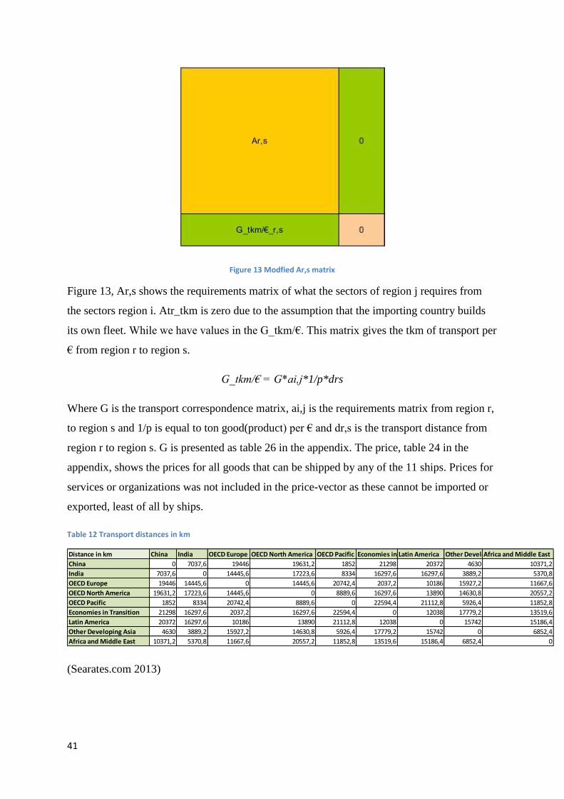
Figure 13 Modfied Ar,s matrix
Figure 13, Ar,s shows the requirements matrix of what the sectors of region j requires from
the sectors region i. Atr_tkm is zero due to the assumption that the importing country builds
its own fleet. While we have values in the G_tkm/€. This matrix gives the tkm of transport per
€ from region r to region s.
G_tkm/€ = G*ai,j*1/p*drs
Where G is the transport correspondence matrix, ai,j is the requirements matrix from region r,
to region s and 1/p is equal to ton good(product) per € and dr,s is the transport distance from
region r to region s. G is presented as table 26 in the appendix. The price, table 24 in the
appendix, shows the prices for all goods that can be shipped by any of the 11 ships. Prices for
services or organizations was not included in the price-vector as these cannot be imported or
exported, least of all by ships.
Table 12 Transport distances in km
(Searates.com 2013)
Distance in km China India OECD Europe OECD North America OECD Pacific Economies in TransitionLatin America Other Developing AsiaAfrica and Middle East
China 0 7037,6 19446 19631,2 1852 21298 20372 4630 10371,2
India 7037,6 0 14445,6 17223,6 8334 16297,6 16297,6 3889,2 5370,8
OECD Europe 19446 14445,6 0 14445,6 20742,4 2037,2 10186 15927,2 11667,6
OECD North America 19631,2 17223,6 14445,6 0 8889,6 16297,6 13890 14630,8 20557,2
OECD Pacific 1852 8334 20742,4 8889,6 0 22594,4 21112,8 5926,4 11852,8
Economies in Transition 21298 16297,6 2037,2 16297,6 22594,4 0 12038 17779,2 13519,6
Latin America 20372 16297,6 10186 13890 21112,8 12038 0 15742 15186,4
Other Developing Asia 4630 3889,2 15927,2 14630,8 5926,4 17779,2 15742 0 6852,4
Africa and Middle East 10371,2 5370,8 11667,6 20557,2 11852,8 13519,6 15186,4 6852,4 0
42
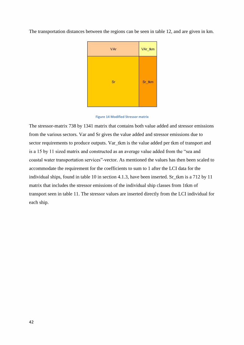
The transportation distances between the regions can be seen in table 12, and are given in km.
Figure 14 Modified Stressor matrix
The stressor-matrix 738 by 1341 matrix that contains both value added and stressor emissions
from the various sectors. Var and Sr gives the value added and stressor emissions due to
sector requirements to produce outputs. Var_tkm is the value added per tkm of transport and
is a 15 by 11 sized matrix and constructed as an average value added from the “sea and
coastal water transportation services”-vector. As mentioned the values has then been scaled to
accommodate the requirement for the coefficients to sum to 1 after the LCI data for the
individual ships, found in table 10 in section 4.1.3, have been inserted. Sr_tkm is a 712 by 11
matrix that includes the stressor emissions of the individual ship classes from 1tkm of
transport seen in table 11. The stressor values are inserted directly from the LCI individual for
each ship.

43
Figure 15 Complete modified system
The final system is illustrated in figure 15. The new big A matrix with the configured
individual a-matrices are given in the yellow square, the configured Value Added in the
orange rectangle, and the green rectangle illustrate the configured stressor matrix.
4.2.2 The Z-matrix
The next step is to construct the Z matrix. Also known as the inter-industry flow-matrix, seen
in figure 16. The Z matrix shows the product flows in euro between the regions and sectors to
satisfy demand. It is therefore different from the A-matrix that it shows total flows, not
coefficient for one unit of output.
44
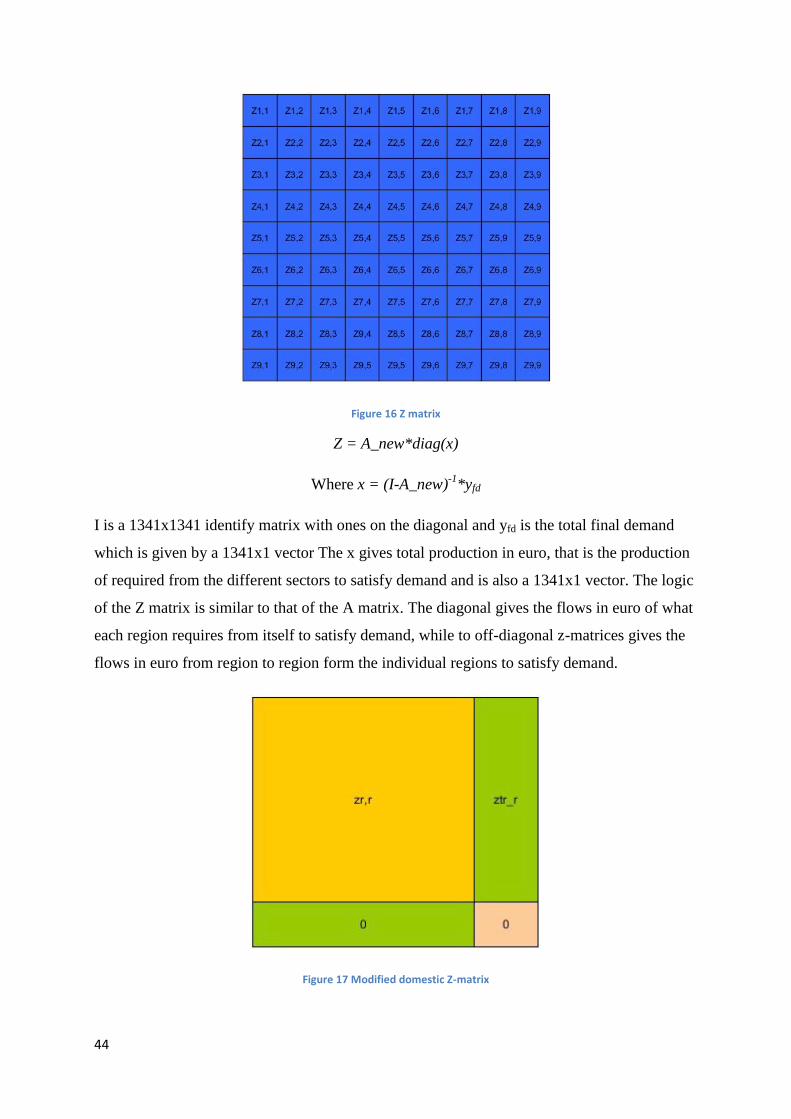
Figure 16 Z matrix
Z = A_new*diag(x)
Where x = (I-A_new)-1
*yfd
I is a 1341x1341 identify matrix with ones on the diagonal and yfd is the total final demand
which is given by a 1341x1 vector The x gives total production in euro, that is the production
of required from the different sectors to satisfy demand and is also a 1341x1 vector. The logic
of the Z matrix is similar to that of the A matrix. The diagonal gives the flows in euro of what
each region requires from itself to satisfy demand, while to off-diagonal z-matrices gives the
flows in euro from region to region form the individual regions to satisfy demand.
Figure 17 Modified domestic Z-matrix
45
Since the Z-matrix is the product of the A-matrix and x, the composition of the z-matrices are
similar to that of the individual A-matrices. figure 17 is an illustration of the composition of
the diagonal Z-matrices, i.e. the flows of what the region require from its own sectors. The
rectangular ztr_r shows the flows required from its own region to construct the fleet
necessary to satisfy the regions import demand while zr,r gives the required flows from the
regions own sectors. The rest is zero as we assume that there is no demand for maritime
transport within a region.
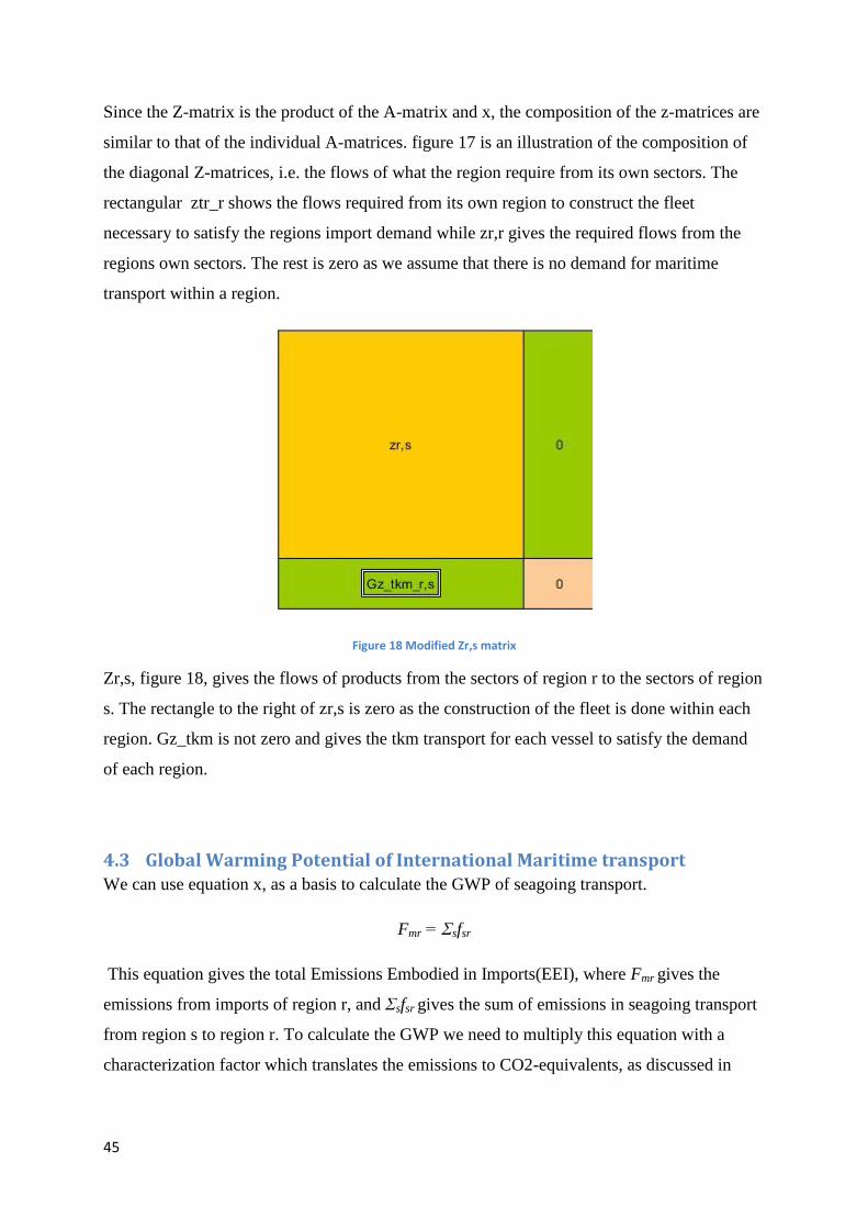
Figure 18 Modified Zr,s matrix
Zr,s, figure 18, gives the flows of products from the sectors of region r to the sectors of region
s. The rectangle to the right of zr,s is zero as the construction of the fleet is done within each
region. Gz_tkm is not zero and gives the tkm transport for each vessel to satisfy the demand
of each region.
4.3 Global Warming Potential of International Maritime transport We can use equation x, as a basis to calculate the GWP of seagoing transport.
Fmr = Ʃsfsr
This equation gives the total Emissions Embodied in Imports(EEI), where Fmr gives the
emissions from imports of region r, and Ʃsfsr gives the sum of emissions in seagoing transport
from region s to region r. To calculate the GWP we need to multiply this equation with a
characterization factor which translates the emissions to CO2-equivalents, as discussed in

46
section 3.1.5 in the methodology chapter. GWP of seagoing transport from importing goods is
thus:
dgwpr gives the GWP of maritime transport due to transport of imported goods.

47
5 Results This section presents the results calculated by using Environmentally Extended Multi-
Regional Input-Output(EE MRIO) approach using the EXIOBASE dataset. The section is
divided into 4 parts; Total Trade flows, Trade flows transported by seagoing vessels, Total
tkm transport between regions, ton km transport by the individual ship classes and global
warming potential of seagoing transport.
5.1 Total Trade flows € Table 13 Regional flows (billion €)
Table 13 shows the total trade flows in billion euro between the different regions. It is found
by summarizing each if the individual region Z matrices into a single value. The diagonal
represents the value flows of what each region requires from itself to satisfy demand, while
the off-diagonal values gives value flows between each region. The columns shows what each
region requires from other regions to satisfy demand of production, i.e. imports, while the
rows shows the value flows that each region exports to satisfy production demand in the other
regions.
To familiarize the reader with the table we can take region 1, China as an example. The
Chinese inter-industry flows between its own sectors summarize 4 229 billion €, while it
require 3 billion € from India70 billion € from OECD Europe, 46 billion € from North
America to satisfy demand for production. China also exports 10 billion€ to India, 29 billion €
to OECD Europe and so on to satisfy production demand.
Region 1 - China Region 2 - India Region 3 - EU Region 4 - NA Region 5 - PAC Region 6 - EIT Region 7 - LA Region 8 - AS Region 9 - AM
Region 1 - China 4 229 10 29 39 81 1 27 13 31
Region 2 - India 3 636 12 11 8 1 3 2 3
Region 3 - EU 70 16 10 717 264 197 51 101 33 106
Region 4 - NA 46 6 268 11 709 194 6 59 39 52
Region 5 - PAC 170 23 200 230 7 190 11 612 135 707
Region 6 - EIT 6 1 75 19 21 409 11 2 11
Region 7 - LA 29 11 86 75 553 7 1 364 48 441
Region 8 - AS 51 3 29 42 103 1 48 664 55
Region 9 - AM 37 14 106 81 691 9 475 60 691
48
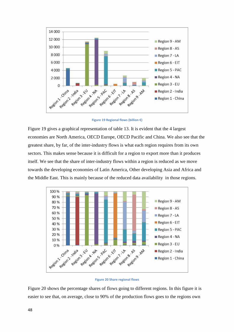
Figure 19 Regional flows (billion €)
Figure 19 gives a graphical representation of table 13. It is evident that the 4 largest
economies are North America, OECD Europe, OECD Pacific and China. We also see that the
greatest share, by far, of the inter-industry flows is what each region requires from its own
sectors. This makes sense because it is difficult for a region to export more than it produces
itself. We see that the share of inter-industry flows within a region is reduced as we move
towards the developing economies of Latin America, Other developing Asia and Africa and
the Middle East. This is mainly because of the reduced data availability in those regions.
Figure 20 Share regional flows
Figure 20 shows the percentage shares of flows going to different regions. In this figure it is
easier to see that, on average, close to 90% of the production flows goes to the regions own
49
sectors. We also see, as mentioned, that the share of inter-industry flows within a region
decreases as we look at the developing economies.
5.2 Shipped trade flow € In this section we study the production flows that are transported between regions by seagoing
vessels. Here, two aspects of seagoing transport is presented. Firstly, the total trade flows
transported by ships are shown, second, this we analyze the extent of ship classes utilized.
5.2.1 Total trade flows shipped between regions
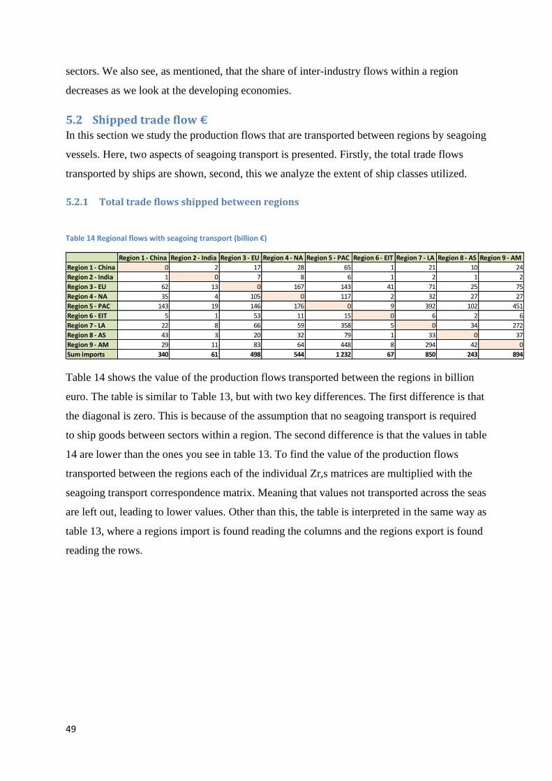
Table 14 Regional flows with seagoing transport (billion €)
Table 14 shows the value of the production flows transported between the regions in billion
euro. The table is similar to Table 13, but with two key differences. The first difference is that
the diagonal is zero. This is because of the assumption that no seagoing transport is required
to ship goods between sectors within a region. The second difference is that the values in table
14 are lower than the ones you see in table 13. To find the value of the production flows
transported between the regions each of the individual Zr,s matrices are multiplied with the
seagoing transport correspondence matrix. Meaning that values not transported across the seas
are left out, leading to lower values. Other than this, the table is interpreted in the same way as
table 13, where a regions import is found reading the columns and the regions export is found
reading the rows.
Region 1 - China Region 2 - India Region 3 - EU Region 4 - NA Region 5 - PAC Region 6 - EIT Region 7 - LA Region 8 - AS Region 9 - AM
Region 1 - China 0 2 17 28 65 1 21 10 24
Region 2 - India 1 0 7 8 6 1 2 1 2
Region 3 - EU 62 13 0 167 143 41 71 25 75
Region 4 - NA 35 4 105 0 117 2 32 27 27
Region 5 - PAC 143 19 146 176 0 9 392 102 451
Region 6 - EIT 5 1 53 11 15 0 6 2 6
Region 7 - LA 22 8 66 59 358 5 0 34 272
Region 8 - AS 43 3 20 32 79 1 33 0 37
Region 9 - AM 29 11 83 64 448 8 294 42 0
Sum imports 340 61 498 544 1 232 67 850 243 894
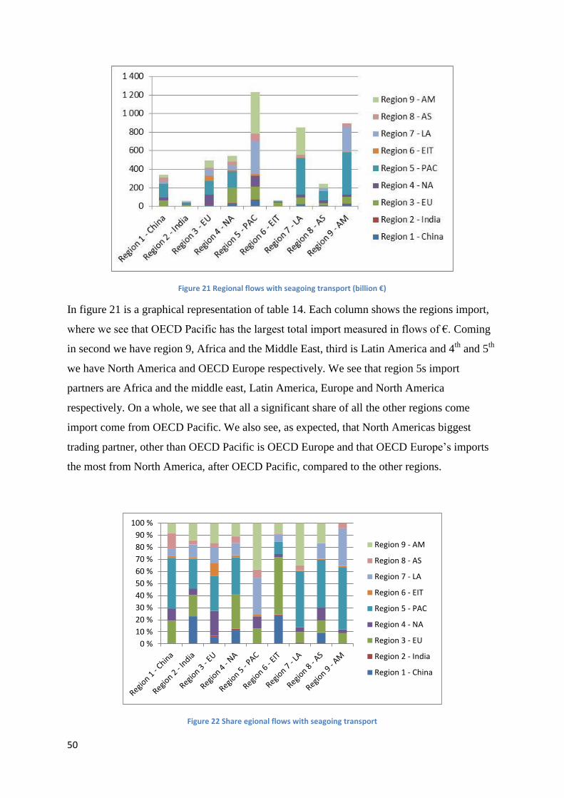
50
Figure 21 Regional flows with seagoing transport (billion €)
In figure 21 is a graphical representation of table 14. Each column shows the regions import,
where we see that OECD Pacific has the largest total import measured in flows of €. Coming
in second we have region 9, Africa and the Middle East, third is Latin America and 4th
and 5th
we have North America and OECD Europe respectively. We see that region 5s import
partners are Africa and the middle east, Latin America, Europe and North America
respectively. On a whole, we see that all a significant share of all the other regions come
import come from OECD Pacific. We also see, as expected, that North Americas biggest
trading partner, other than OECD Pacific is OECD Europe and that OECD Europe’s imports
the most from North America, after OECD Pacific, compared to the other regions.
Figure 22 Share egional flows with seagoing transport
0 %
10 %
20 %
30 %
40 %
50 %
60 %
70 %
80 %
90 %
100 %
Region 9 - AM
Region 8 - AS
Region 7 - LA
Region 6 - EIT
Region 5 - PAC
Region 4 - NA
Region 3 - EU
Region 2 - India
Region 1 - China

51
In figure 22 we see the trade partners for each region as shares of total import. On a whole we
see that OECD Pacific is the greatest exporter and the major import partner of the other
regions. The exception is “Economies in Transition” where the largest import share is from
OECD Europe and China. For India the import from OECD Pacific is only slightly larger than
their import from China and in North America the import from OECD Pacific and OECD
Europe is about the same size, covering nearly 60% of its total imports. India and Economies
in transition have the lowest import share of all the regions and most of EITs exports are
bound to Europe. Africa and the Middle East is an interesting region where as most of their
exports, both as shares and in total goes towards OECD Pacific and Latin America, and then
has a relative constant average import share of 12-15% in the other regions.
5.2.2 Total trade flows between regions, vessel resolution
Table 15 Regional tradeflows by vessel type (million €)
In table 15 we see the total exports of each region broken down to ship class resolution in
million euro. To familiarize the reader with the table we can again use China as an example.
The value of the production flows exported using a large dry bulk carrier is 5 123 million
euro, containerized cargo exported from China has a value of 111 782 million euro while
value products transported by Reefer vessels are 6 441 million euro.
Region 1 - China Region 2 - India Region 3 - EU Region 4 - NA Region 5 - PAC Region 6 - EIT Region 7 - LA Region 8 - AS Region 9 - AM sum
Large Dry Bulk 5 123 354 502 2 868 17 511 8 899 12 846 1 952 18 093 68 149
Dry Bulk 14 545 7 387 54 848 35 938 206 548 29 235 135 627 26 384 166 075 676 587
General Cargo 5 279 809 24 460 21 888 35 237 5 397 26 760 9 768 28 302 157 899
Container 111 782 10 506 274 416 137 405 598 317 10 913 268 252 125 093 312 615 1 849 299
Reefer 6 441 1 596 25 919 18 790 71 736 3 346 55 491 9 446 64 035 256 799
RoRo 8 011 1 187 77 387 48 937 84 388 2 257 19 509 12 408 20 641 274 724
Crude Oil 4 361 0,10 13 821 9 740 134 845 18 344 120 531 15 866 151 274 468 781
Chemical 1 301 140 18 047 14 222 133 647 9 352 94 633 18 193 111 642 401 177
Oil Products 10 042 5 267 107 972 58 203 110 409 8 115 53 412 17 839 61 734 432 993
LNG 508 17 1 287 514 15 864 3 370 15 273 7 460 18 676 62 969
LPG 0,04 0,04 95 56 28 068 29 21 996 2 618 25 890 78 752,53
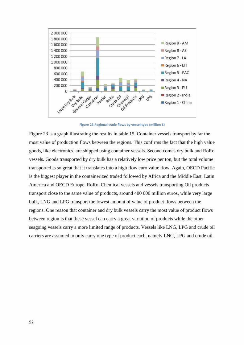
52
Figure 23 Regional trade flows by vessel type (million €)
Figure 23 is a graph illustrating the results in table 15. Container vessels transport by far the
most value of production flows between the regions. This confirms the fact that the high value
goods, like electronics, are shipped using container vessels. Second comes dry bulk and RoRo
vessels. Goods transported by dry bulk has a relatively low price per ton, but the total volume
transported is so great that it translates into a high flow euro value flow. Again, OECD Pacific
is the biggest player in the containerized traded followed by Africa and the Middle East, Latin
America and OECD Europe. RoRo, Chemical vessels and vessels transporting Oil products
transport close to the same value of products, around 400 000 million euros, while very large
bulk, LNG and LPG transport the lowest amount of value of product flows between the
regions. One reason that container and dry bulk vessels carry the most value of product flows
between region is that these vessel can carry a great variation of products while the other
seagoing vessels carry a more limited range of products. Vessels like LNG, LPG and crude oil
carriers are assumed to only carry one type of product each, namely LNG, LPG and crude oil.

53
Figure 24 Share of regional trade flows by vessel type
Looking at figure 24 and the shares of the regions utilizing the various vessels classes to
transport the value flows of their products between regions we see that OECD Pacific, Latin
America, and Africa and the Middle East dominate the figure. Europe has relative larger share
on transport using RoRo vessels and Oil product vessels, while not surprisingly Africa and the
Middle East are one of the largest Crude oil exporters.
5.3 Total ton kilometer transport In this section we move away from the value of production flows between the regions and
focus on the total ton kilometer transport. The first part focus on the total ton km transport
between the regions, their exports and imports. The next section breaks down the trade to ship
class resolution and show the total export of each region by vessel.
5.3.1 Ton kilometer transport between regions
Table 16 Interregional seagoing transport (billion tkm)
Table 16 shows the total transport between the regions in billion ton kilometer. As in table 15
the diagonal is zero due to the assumption that there is no seagoing transport within a region.
Region 1 - China Region 2 - India Region 3 - EU Region 4 - NA Region 5 - PAC Region 6 - EIT Region 7 - LA Region 8 - AS Region 9 - AM
Region 1 - China 0 20 216 292 103 17 285 40 166
Region 2 - India 9 0 86 93 49 15 46 5 14
Region 3 - EU 684 295 0 2 143 2 883 68 677 297 730
Region 4 - NA 466 121 1 235 0 1 208 26 481 254 435
Region 5 - PAC 186 202 2 227 1 106 0 301 7 715 500 4 995
Region 6 - EIT 132 21 108 150 393 0 80 23 82
Region 7 - LA 408 207 602 834 7 529 104 0 507 4 075
Region 8 - AS 126 16 171 234 413 16 443 0 223
Region 9 - AM 277 89 945 1 451 5 355 185 4 404 289 0
Sum imports 2 289 970 5 590 6 303 17 934 733 14 130 1 915 10 720

54
The columns show how much ton kilometer transport of import that is required from the other
regions while the rows show the export in ton kilometer transport.
Figure 25 Interregional seagoing transport (billion tkm)
Figure 25 shows the values of table 15 graphically. We see that OECD Pacific has the largest
import measured in ton km, followed by Latin America and Africa and the Middle east. The
total import of region 5 measured in ton km is massive, 17 934 billion ton km, and so is the
ton km of imports of EU and North America as well. As we saw in figure 23 OECD Pacific’s
major trading partners are Latin America and Africa and the Middle East. OECD Europe is
North Americas major trading partner, while Europe’s import from OECD Pacific is twice as
large as their import from North America measured in ton km transport. In figure 23 looking
at the value of the production flows rather than the ton km transport we saw that the share of
Europe’s imports from North America and OECD Pacific where close to the same value. One
reason to why we see this difference lies in the distance between the ports. OECD Pacific is
further away from Europe than North America is and the added distance increases the share of
imports from OECD Pacific relative to the import shares from North America.
The total seagoing transport between the regions account for 60 000 billion ton km, a total
that is lower than the 71 000 billion ton km, reported by UNCTADs review of Maritime
transport 2012. One explanation to this deviation is due of the assumption of no maritime
transport within each region. Region 5, OECD Pacific are a model of Japan, South Korea,
Australia and New Zealand. Japan is the world’s biggest steel producers and is together with
South Korea one of the world’s largest ship builder. Australia on the other hand is the world’s
largest exporters of coal and iron ore, and Japan is one of Australia’s greatest export markets
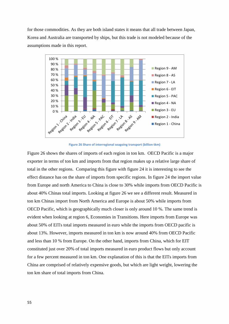
55
for those commodities. As they are both island states it means that all trade between Japan,
Korea and Australia are transported by ships, but this trade is not modeled because of the
assumptions made in this report.
Figure 26 Share of interregional seagoing transport (billion tkm)
Figure 26 shows the shares of imports of each region in ton km. OECD Pacific is a major
exporter in terms of ton km and imports from that region makes up a relative large share of
total in the other regions. Comparing this figure with figure 24 it is interesting to see the
effect distance has on the share of imports from specific regions. In figure 24 the import value
from Europe and north America to China is close to 30% while imports from OECD Pacific is
about 40% Chinas total imports. Looking at figure 26 we see a different result. Measured in
ton km Chinas import from North America and Europe is about 50% while imports from
OECD Pacific, which is geographically much closer is only around 10 %. The same trend is
evident when looking at region 6, Economies in Transitions. Here imports from Europe was
about 50% of EITs total imports measured in euro while the imports from OECD pacific is
about 13%. However, imports measured in ton km is now around 40% from OECD Pacific
and less than 10 % from Europe. On the other hand, imports from China, which for EIT
constituted just over 20% of total imports measured in euro product flows but only account
for a few percent measured in ton km. One explanation of this is that the EITs imports from
China are comprised of relatively expensive goods, but which are light weight, lowering the
ton km share of total imports from China.
0 %
10 %
20 %
30 %
40 %
50 %
60 %
70 %
80 %
90 %
100 %
Region 9 - AM
Region 8 - AS
Region 7 - LA
Region 6 - EIT
Region 5 - PAC
Region 4 - NA
Region 3 - EU
Region 2 - India
Region 1 - China
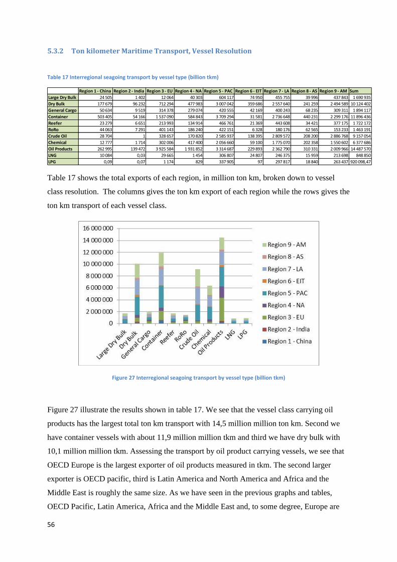
56
5.3.2 Ton kilometer Maritime Transport, Vessel Resolution
Table 17 Interregional seagoing transport by vessel type (billion tkm)
Table 17 shows the total exports of each region, in million ton km, broken down to vessel
class resolution. The columns gives the ton km export of each region while the rows gives the
ton km transport of each vessel class.
Figure 27 Interregional seagoing transport by vessel type (billion tkm)
Figure 27 illustrate the results shown in table 17. We see that the vessel class carrying oil
products has the largest total ton km transport with 14,5 million million ton km. Second we
have container vessels with about 11,9 million million tkm and third we have dry bulk with
10,1 million million tkm. Assessing the transport by oil product carrying vessels, we see that
OECD Europe is the largest exporter of oil products measured in tkm. The second larger
exporter is OECD pacific, third is Latin America and North America and Africa and the
Middle East is roughly the same size. As we have seen in the previous graphs and tables,
OECD Pacific, Latin America, Africa and the Middle East and, to some degree, Europe are
Region 1 - China Region 2 - India Region 3 - EU Region 4 - NA Region 5 - PAC Region 6 - EIT Region 7 - LA Region 8 - AS Region 9 - AM Sum
Large Dry Bulk 24 505 1 402 12 064 40 303 604 117 74 950 455 755 39 996 437 843 1 690 935
Dry Bulk 177 679 96 232 712 294 477 983 3 007 042 359 686 2 557 640 241 259 2 494 589 10 124 402
General Cargo 50 634 9 519 314 378 279 074 420 555 42 169 400 243 68 235 309 311 1 894 117
Container 503 405 54 166 1 537 090 584 843 3 709 294 31 581 2 736 648 440 231 2 299 176 11 896 436
Reefer 23 279 6 651 213 993 134 914 466 761 21 369 443 608 34 421 377 175 1 722 172
RoRo 44 063 7 291 401 143 186 240 422 151 6 328 180 176 62 565 153 233 1 463 191
Crude Oil 28 704 1 328 657 170 820 2 585 937 138 395 2 809 572 208 200 2 886 768 9 157 054
Chemical 12 777 1 714 302 006 417 400 2 056 660 59 100 1 775 070 202 358 1 550 602 6 377 686
Oil Products 262 995 139 472 3 925 584 1 931 852 3 314 687 229 893 2 362 790 310 331 2 009 966 14 487 570
LNG 10 084 0,03 29 665 1 454 306 807 24 807 246 375 15 959 213 698 848 850
LPG 0,09 0,07 1 174 829 337 905 97 297 817 18 840 263 437 920 098,47

57
the biggest importers and exporters, both in terms of euro value of production flows between
the regions and in tkm transport. China and North America is not as dominating as first
anticipated and the author expected to so China as a more dominant force on the export side
and North America a more dominant player considering imports from other nations,
especially from China.
Let’s take a minute to compare figure 27 with figure 23 in 5.3.2. Figure 27, as we just saw,
illustrate the exports, given in tkm, of each region broken down to ship class resolution.
Figure 27, on the other hand, show the the exports of each region, given in euro value of the
production flows, of each region. In figure 23 we saw that containerized shipping transport,
by far, the most production flows measured in euro. Dry bulk comes in second while the other
vessels, RoRo, chemical and oil products, in particular, carry relatively the same amount of
value between the regions. In figure 27, assessing the tkm transport, we see a completely
different picture. Here, Oil product carriers transport has the highest tkm transport with 14
487 570 million tkm. Container and Dry bulk have the second and third largest tkm transport
with roughly 12 000 000 and 10 000 000 million tkm respectively. A reasonable explanation
for these results lies in transportation distance and tonnage. Apparently, the euro value of
products being shipped between the regions using oil product carriers, RoRo vessels and
vessels who carry chemicals is much less than the combined tonnage and transport distance of
the products.
Figure 28 Interregional seagoing transport by vessel type (billion tkm)
Figure 28 shows the share countries utilizing the different vessel classes to export their goods.
Again we see that OECD Pacific, Latin America and Africa and the Middle East, together

58
with OECD Europe dominate the figure. Most of Europe’s export is carried using RoRo and
Oil product carriers while the exports of OECD Pacific, Latin America and Africa and the
Middle East is distributed relatively evenly across all the vessel classes.
Looking at the share of exports transported by container vessels, we see a relatively high
share is allocated to OECD Europe while China barely registers. We know that China exports
a larger volume by Container than what Europe does, but the assumption that the price of the
exports are equal in all regions changes this. The € value of Europe’s container export is
higher than the € value of Chinas Container export 111 000 million € to 275 000 million €,
respectively, so assuming the same price for the two export flows translate into lower total
tkm by container export from China than from Europe, giving somewhat distorted results.
5.4 Environmental Impacts This section focus on assessing the Global Warming Potential(GWP), expressed in kg CO2-
equivalents, of international maritime transport and international trade. The first part show the
total GWP of all the activity, export and import between the 9 regions, the second part gives
the GWP of international maritime transport between the regions while the third part gives the
GWP of the total imports of each region distributed on the 11 ship classes.
5.4.1 Total Global Warming Potential
Table 18 Total GWP (Billion ton CO2-eq)
Table 18 shows the total GWP of all the activity, export and import between the regions in
billion ton CO2-equivalents. The sum of GWP embedded in the imports of each region is seen
in the bottom row of the table. To use China as an example, we that the total GWP embedded
in the regions import is 866 956 billion CO2-equivalents. The GWP from the regions demand
from its own sectors is given on the diagonal of the table, the regions export is given in the
rows while the imports are given on the columns.
Region 1 - China Region 2 - India Region 3 - EU Region 4 - NA Region 5 - PAC Region 6 - EIT Region 7 - LA Region 8 - AS Region 9 - AM
Region 1 - China 9 049 621 91 116 117 370 172 547 286 000 5 974 99 841 41 590 88 085
Region 2 - India 22 572 2 264 491 45 204 41 902 30 876 4 027 15 882 6 375 11 393
Region 3 - EU 62 155 17 663 4 585 779 209 538 174 268 27 710 72 456 22 444 63 976
Region 4 - NA 61 859 9 246 163 541 7 503 037 158 202 4 762 50 228 28 253 38 572
Region 5 - PAC 300 627 40 323 198 795 211 800 3 890 566 10 570 513 309 93 051 460 889
Region 6 - EIT 68 633 12 780 334 333 102 400 137 653 1 721 506 58 063 17 133 48 543
Region 7 - LA 172 296 28 339 116 170 120 593 654 390 7 577 1 632 708 57 476 350 928
Region 8 - AS 55 259 7 702 40 403 52 675 153 146 1 815 80 626 708 186 72 202
Region 9 - AM 123 556 23 815 132 317 139 735 689 548 8 966 408 849 59 952 1 138 493
sum imports 866 956 230 983 1 148 133 1 051 191 2 284 084 71 402 1 299 253 326 273 1 134 588
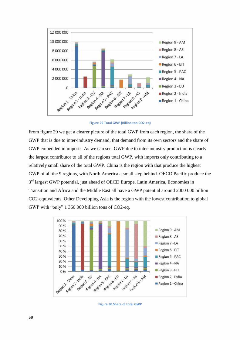
59
Figure 29 Total GWP (Billion ton CO2-eq)
From figure 29 we get a clearer picture of the total GWP from each region, the share of the
GWP that is due to inter-industry demand, that demand from its own sectors and the share of
GWP embedded in imports. As we can see, GWP due to inter-industry production is clearly
the largest contributor to all of the regions total GWP, with imports only contributing to a
relatively small share of the total GWP. China is the region with that produce the highest
GWP of all the 9 regions, with North America a small step behind. OECD Pacific produce the
3rd
largest GWP potential, just ahead of OECD Europe. Latin America, Economies in
Transition and Africa and the Middle East all have a GWP potential around 2000 000 billion
CO2-equivalents. Other Developing Asia is the region with the lowest contribution to global
GWP with “only” 1 360 000 billion tons of CO2-eq.
Figure 30 Share of total GWP

60
In figure 30 we clearly see that the inter-industry demands within each region is by far the
biggest contributor to the total GWP. The only real exception is Africa and the Middle East
where the share of GWP from production within the region is roughly the same size of GWP
due to imports.
5.4.2 Global Warming Potential from Maritime Transport
Table 19 GWP from maritime transport (thousand ton CO2-eq)
Table 19 gives the GWP of maritime transport between the regions in thousand tons. Since it
is assumed that each region builds in own fleet required to import the goods they demand, we
see the GWP of construction required vessels on the diagonal of the table. The bottom row
gives the total GWP from maritime transport due to each regions import demand. The GWP
of the regions import is given in the columns while the GWP due to export is read from the
rows. OECD Pacific has the largest GWP from building its required fleet with an emission of
109 858 thousand tons of CO2-equivalents, second comes Latin America with 54 440
thousand tons of CO2 equivalents while OECD Europe and North America have a GWP
between 8 500 and 6 150 thousand tons of CO2-equivalents, respectively.
Region 1 - China Region 2 - India Region 3 - EU Region 4 - NA Region 5 - PAC Region 6 - EIT Region 7 - LA Region 8 - AS Region 9 - AM
Region 1 - China 826 622 5 702 8 964 6 317 381 6 234 1 145 3 766
Region 2 - India 375 42 1 955 2 213 1 306 252 887 140 402
Region 3 - EU 26 555 8 221 8 491 70 258 69 284 1 776 21 568 7 784 17 811
Region 4 - NA 15 459 4 577 33 060 6 143 35 182 1 117 13 511 5 774 10 462
Region 5 - PAC 22 862 13 836 121 126 85 739 109 858 5 984 152 157 19 849 94 542
Region 6 - EIT 4 831 833 5 670 3 859 9 457 140 3 272 758 2 601
Region 7 - LA 38 089 14 454 58 168 76 702 225 281 3 182 54 440 21 367 81 202
Region 8 - AS 5 234 891 8 494 10 976 15 322 390 9 861 946 5 877
Region 9 - AM 27 890 8 426 66 942 109 719 171 361 3 615 97 612 14 897 38 076
sum import 141 294 51 860 301 117 368 430 533 510 16 697 305 101 71 714 216 662

61
Figure 31 GWP from maritime transport (thousand ton CO2-eq)
From figure 31 it becomes evident that OECD Pacific leads the way in terms of GWP from
maritime transport and fleet construction with a total GWP of roughly 630 000 thousand tons
of CO2-equivalents, of which 533 515 thousand tons are due to seagoing transportation of the
regions imports. The bulk of GWP from OECD Pacific imports are due to seagoing
transportation of goods from Latin America and Africa and the Middle East, and they account
for 225 000 and 171 000 thousands of tons, respectively.
North America comes in second with a GWP of about 390 000 thousand tons CO2-
equivalents where 368 000 thousand tons of CO2-eq are due to seagoing transportation of
imports, just ahead of Latin America. OECD Europe have a total GWP of 310 000 thousand
tons where 301 000 thousand tons are a consequence of the seagoing transport of the regions
imports. The share of GWP of maritime transport due to imports from OECD Pacific is quite
significant for all the regions. The same is evident for Africa and the Middle East and Latin
America but on a smaller scale.
The bulk of GWP due to seagoing transport of Europe’s exports are allocated to North
America and OECD Pacific at 70 000 thousand tons of CO2-equivalents.

62
Figure 32 Share of GWP from maritime transport
Assessing figure 32 we see that Latin America and Africa and the Middle East both contribute
to a rather large share of each of the other regions GWP imports. This may be due to their
geographic position, relatively far away from the other regions. OECD Pacific has biggest
share of GWP due to maritime transportation of imported goods in all regions except for
China. This may be a consequence of the two regions close geographical proximity. GWP due
to seagoing transport of goods imported from Europe contribute to about 15 % on average in
each of the regions.
5.4.3 Global Warming Potential embodied in trade, vessel resolution
Table 20 GWP by vessel type (Thousand ton CO2-eq)
Table 20 shows the GWP, in thousand ton, of total seagoing transport of imports to each
region distributed on the 11 vessel classes. The rows show the GWP of each vessel to the
different regions while the last column show the total GWP of each vessel. To give an
example, the consequence of Chinese import demand is a GWP 5 226 thousand tons from Dry
Bulk carriers, 6 517 thousand tons from General Cargo vessels and 26 447 thousand tons from
Container vessels, given in CO2-equivalents. The sum of GWP of transport by Dry Bulk
Region 1 - China Region 2 - India Region 3 - EU Region 4 - NA Region 5 - PAC Region 6 - EIT Region 7 - LA Region 8 - AS Region 9 - AM Sum
Large Dry Bulk 335 91 1 443 616 3 711 770 2 310 416 1 744 11 436
Dry Bulk 5 226 3 543 11 669 12 024 36 694 1 791 24 699 4 336 17 828 117 809
General Cargo 6 517 4 012 12 155 10 997 32 596 771 17 912 4 028 13 094 102 082
Container 26 447 6 212 30 351 39 215 105 942 2 270 72 020 13 060 53 121 348 637
Reefer 4 411 609 9 808 12 982 48 042 1 561 28 653 4 106 19 586 129 757
RoRo 922 133 1 308 2 017 2 627 131 1 963 321 1 447 10 869
Crude Oil 58 793 23 596 180 206 226 999 171 145 5 539 70 602 26 213 49 646 812 738
Chemical 4 837 1 426 10 492 13 394 28 964 523 18 428 3 921 14 697 96 681
Oil Products 31 484 11 337 34 719 43 939 88 365 2 510 58 271 13 307 38 198 322 129
LNG 928 338 3 430 1 936 7 224 572 4 892 895 3 453 23 668
LPG 1 395 563 5 537 4 310 8 201 260 5 351 1 112 3 848 30 576

63
carriers are 117 809 thousand tons, for General Cargo vessel its 102 082 thousand tons and for
Container vessels its 348 637 thousand tons of CO2-equivalents.
Figure 33 GWP by vessel type (Thousand ton CO2-eq)
Figure 33 shows that its Crude oil vessels that have the highest total GWP with 812 738
thousand tons of CO2-equivalents. OECD Europe, North America and OECD Pacific as the
regions with the highest share of oil imports, with a GWP of 180 206, 226 999 and 171 145
thousand tons of CO2-equivalents, respectively. Comparing the total GWP of Crude oil
carriers with the GWP reported by Lindstad et.al 2012 in the paper “The Importance of
economies of scale for reductions in greenhouse gas emissions from shipping”, from table 21,
Crude Oil carriers emit roughly 98 million tons of CO2-equivalents each year, which is 8
times lower than the GWP obtained in this study. The emission intensities for Crude Oil
Carriers used in this report are the same as the one found in the Lindstad et.al 2012 paper and
it is therefore probable that the EXIOBASE dataset estimate a higher trade of crude oil in
combination with a more diverse Crude Oil Carrying fleet in the Lindstad paper, with larger
ships that has lower emissions per ton km transport. Seagoing transport of containerized
goods have the second largest GWP after Crude Oil carriers, with transport of Oil products
not far behind.
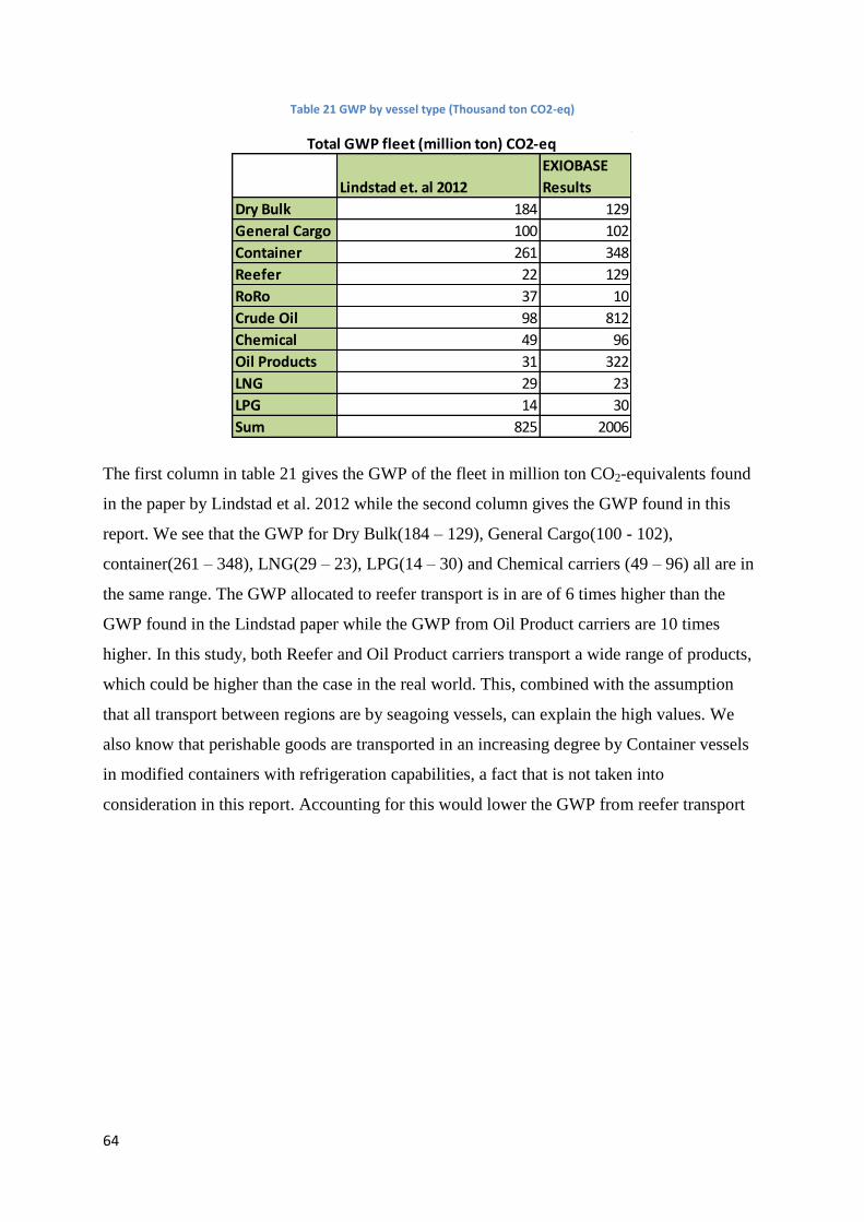
64
Table 21 GWP by vessel type (Thousand ton CO2-eq)
The first column in table 21 gives the GWP of the fleet in million ton CO2-equivalents found
in the paper by Lindstad et al. 2012 while the second column gives the GWP found in this
report. We see that the GWP for Dry Bulk(184 – 129), General Cargo(100 - 102),
container(261 – 348), LNG(29 – 23), LPG(14 – 30) and Chemical carriers (49 – 96) all are in
the same range. The GWP allocated to reefer transport is in are of 6 times higher than the
GWP found in the Lindstad paper while the GWP from Oil Product carriers are 10 times
higher. In this study, both Reefer and Oil Product carriers transport a wide range of products,
which could be higher than the case in the real world. This, combined with the assumption
that all transport between regions are by seagoing vessels, can explain the high values. We
also know that perishable goods are transported in an increasing degree by Container vessels
in modified containers with refrigeration capabilities, a fact that is not taken into
consideration in this report. Accounting for this would lower the GWP from reefer transport
EXIOBASE
Lindstad et. al 2012 Results
Dry Bulk 184 129
General Cargo 100 102
Container 261 348
Reefer 22 129
RoRo 37 10
Crude Oil 98 812
Chemical 49 96
Oil Products 31 322
LNG 29 23
LPG 14 30
Sum 825 2006
Total GWP fleet (million ton) CO2-eq

65
Figure 34 Share of GWP by vessel type
From figure 34 we see that the GWP from seagoing transport of imports are relatively similar
on the different vessels. Europe, North America and OECD Pacific are the three regions that
have the highest GWP from importing crude oil. Latin America and Africa and the Middle
East have relatively similar share across the board, 20% and 15 % respectively.
5.4.4 GWP from Maritime Transportation vs. Total GWP
Table 22 Comparison of GWP by region (million ton CO2-eq)
Table 22 gives the GWP, in million ton CO2-equivalents, of total imports, i.e. the emissions of
CO2-equivalents from producing the imported goods, the GWP of seagoing transport required
to transport said imported goods to the region and the share of GWP of seagoing transport of
the GWP of total imports. North America, OECD Europe, OECD Pacific and Latin America
are the regions with the highest GWP from seagoing transportation with 368, 301, 534 and
305 million tons of CO2-equivalents, respectively. However, the GWP share of seagoing
transport is microscopic for all regions, when it should be between 3%-6%(UNCTAD 2012).
Million ton CO2-eq Region 1 - China Region 2 - India Region 3 - EU Region 4 - NA
Total imports 867 424 277 231 023 142 1 149 752 773 1 054 777 245
Total seagoing trans. 141 52 301 368
GWP share 0,0000163 % 0,0000224 % 0,0000262 % 0,0000349 %
Region 5 - PAC Region 6 - EIT Region 7 - LA Region 8 - AS Region 9 - AM
2 284 804 481 71 428 816 1 299 654 682 326 392 031 1 134 864 038
534 17 305 72 217
0,0000234 % 0,0000234 % 0,0000235 % 0,0000220 % 0,0000191 %

66
The GWP of seagoing transport is calculated to be between 825 and 1 0046 million tons(IMO
2009, Lindstad, Asbjørnslett et al. 2012) and contribute to between 3%-5% of total world
GWP(IMO 2009, Shipbuilding 2010, Lindstad, Asbjørnslett et al. 2011, Lindstad,
Asbjørnslett et al. 2012, UNCTAD 2012).
Figure 35 Comparison of GWP by region (million ton CO2-eq)
From figure 35 it is evident that OECD Pacific has the highest GWP embedded in imports of
all the regions. Second comes Latin America, closely followed by OECD Europe, North
America, and Africa and the Middle East. GWP from seagoing transport as share barely
registers in the figure.
Table 23 Comparison of Total GWP (million ton CO2-eq)
The same trend can be seen in table 23. Total world GWP is 40 907 249 753 million tons
CO2-equivalents while GWP from Maritime transport is 2006 million tons CO2-equivalents.
The share of total GWP from maritime transport is 0,0000049%, not even close to 3,3% share
reported by IMO 2009(IMO 2009). Models of global production, trade and economic activity
like the EXIOBASE dataset are extremely useful when it comes to assess inter-industry
requirements between sectors from different regions or to try to get an image of the GWP of
seagoing transport. The model is constructed by putting together millions of different pieces
of information into a coherent system. Some of the pieces are accurate, measured tables of
(million ton CO2-eq) GWP Share of seagoing transport
World 40 907 249 753 on World GWP
Maritime Transport 2 006 0,0000049 %

67
flows that matches those of the real world, but most of the information that the EXIOBASE
dataset builds on are based on many assumptions and approximations. This leads to
inaccuracies when the entire EXIOBASE dataset is used to calculate total GWP of all
economic activities, which in this case resulted in a GWP that was too high.
6 Discussion The main objective of this report was to improve the representation of international maritime
transport in the EXIOBASE dataset by integrating 11 individual ship class inventories into the
MRIO dataset. This report then calculated the global warming potential of seagoing transport
as a consequence of interregional trade by an Environmentally Extended Multi-Regional
Input-Output(EE MRIO) approach.
The results demonstrate that the total GWP from international maritime trade is calculated to
2006 million tons of CO2-equivalents. This is about twice as much as the GWP that is
reported by IMO and H.Lindstad(IMO 2009, Lindstad, Asbjørnslett et al. 2012, UNCTAD
2012) which is calculated to between 825 and 1 046 million tons of CO2-equivalents. This
report assumes that all trade between the 9 world regions is transported by seagoing vessels
and so excludes airfreight, rail and road transportation. The consequence of this assumption is
higher GWP from maritime transport, which the results demonstrate. On the other hand, it is
also assumed that there is no seagoing transportation within each region. This does not have
much effect of inter-industry trade in OECD Europe and North America for example, but for
EXIOBASE regions like OECD Pacific, which is comprised of island states such as Japan,
Australia and New Zealand, the effect on GWP might be bigger. As discussed in section
5.3.1, the trade within the OECD Pacific region is significant, and contribute to balance out
some of the higher GWP due to assumption of seagoing transport being the only form of
transport between regions.
The results demonstrate that North America, OECD Europe and OECD Pacific have the
highest GWP embodied in imports from seagoing trade. This is expected as these are all
regions of highly industrialized countries with a high level of household consumption and
manufacturing industries with a high import demand for raw materials from less developed
regions. It is interesting to note that Latin America actually has a higher GWP embodied in
imports from maritime transport than OECD Europe. This may be a result of extensive
transportation distances, seeing that the bulk of the regions imports are transported all the way

68
from Europe, China and OECD Pacific, but it also implies a higher household and industry
demand than what I expected.
This report assumes that each region builds the fleet required to transport the amount import
demanded by its industries. The GWP of this shipbuilding is seen on the diagonal of table 19
in section 5.4.1 and reflects the ton km of import demanded in each region.
This study found that seagoing transport by crude oil carriers produced the biggest GWP and
is responsible for the emissions of 812 million tons of CO2-equivalents, 40% of the total GWP
of 2006 million tons CO2-equivalents. This GWP is 8 times higher than the one reported by
(Lindstad, Asbjørnslett et al. 2012) at 98 million tons CO2-equivalents. As was discussed in
section 5.4.3 it is probable that the EXIOBASE dataset estimate a higher trade of crude oil in
combination with a more diverse Crude Oil Carrying fleet in the Lindstad.et al paper, with
larger ships that has lower emissions per ton km transport than the one used in this report. The
GWP of the other ship classes where comparable with the Lindstad et. al paper. The
exceptions, other than crude oil carriers, are reefer vessels and oil product carriers who had
20% higher GWP. It is assumed that crude oil carriers only transport crude oil with OECD
Europe, North America and OECD Pacific as largest importers and Africa and the Middle
East as the largest exporter of the product.
Looking at the share of exports transported by container vessels in section 5.3.2, figure 27, we
see a relatively high share is allocated to OECD Europe while China barely registers. We
know that China exports a larger volume by Container than what Europe does, but the
assumption that the price of the exports are equal in all regions changes this. The € value of
Europes container export is higher than the € value of Chinas Container export 111 000
million € to 275 000 million €, respectively, so assuming the same price for the two export
flows translate into lower total tkm by container export from China than from Europe, giving
somewhat distorted results. It is therefore suggested that any future study of seagoing
transport using the EE MRIO EXIOBASE dataset employ differentiated price tables to further
improve the model.
As mentioned in the introduction maritime transport represent approximately 3,3 % of world
GWP. This report found that only 0,0000049% of world GWP is due to seagoing transport
operations, a quite significant difference. This difference, as discussed in section 5.4.4, might
be a consequence of how the EXIOBASE dataset is constructed.

69
This report finds that the total ton km transported by seagoing vessels is lower than what is
found in the study by (Lindstad, Asbjørnslett et al. 2012) and the UNCTAD Review of
maritime transport 2012. This result is surprising, considering the fact that this analysis
assumes that all interregional trade is transported by sea. These contradictions are not
properly assessed in this report, and I propose that they are considered in further studies.
A key component of this report is the correspondence matrix, i.e. the G matrix described in
section 4.2.1, that I developed in dialogue with co-supervisor Haakon Lindstad. The G matrix
allocates products and goods to the vessels that carry them, and while it is assumed that some
vessels are capable of carrying several different types of goods, such as container vessels, it is
assumed that no two vessels carry the same good. This is a simplification and we know
different types of ships can have overlapping carrying capabilities(Haakon Lindstad 2012).
The most versatile of all ships described in this report is the container vessel, which can carry
anything from consumer goods to chemicals, perishable products, cars to cardboard all on the
same voyage. Other vessels, such as general cargo vessels, bulk carriers and RoRo vessels can
all carry some of the same goods(Haakon Lindstad 2012). It is possible to improve the
accuracy of the model if data on the distribution of overlapping transport where researched
and collected, which the author encourages.
This report has also assumed that the carrying capacity of each vessel is utilized 100%. The
utilization factor when loaded can vary greatly between vessels, from up to 98% for crude oil
tankers down to 70% utilization for certain container vessels. Neither is duration and number
of ballast voyages per vessel, which would further reduce the carrying efficiency of each
vessel and most likely increase GWP from seagoing trade if these factors were accounted for
in the model.
January 1st of this year, mandatory new measures aimed at improving the energy efficiency
of international shipping and reduce emissions of greenhouse gasses entered into force.
Energy Efficiency Design Index (EEDI), is made mandatory for new ships, and the Ship
Energy Efficiency Management Plan (SEEMP) for all ships (IMO 2009). The EEDI is a non-
prescriptive, performance-based mechanism that leaves the choice of technologies to use in a
specific ship design to the industry. As long as the required energy-efficiency level is reached,
ship designers and builders would be free to use the most cost-efficient solutions for the ship
to comply with the regulations. The SEEMP establishes a mechanism for operators to
improve the energy efficiency of ships. Ships are required to keep on board a ship specific

70
Ship Energy Efficiency Management Plan (SEEMP). It is indicated that these measures will
reduce the ton km transport by almost 40% versus “business as usual” in 2050, and that EEDI
will contribute to 75% of the reduction(Lindstad, Asbjørnslett et al. 2012). It would be
interesting to try to implement the effects of these measures into to improved MRIO dataset to
see if the GWP is indeed reduced.
71
7 Conclusion This report has improved the EXIOBASE dataset by integrating life cycle inventories of 11
individual ship classes. GWP from seagoing transport was calculated by performing an
Environmentally Extended Multi-Regional Input-Output(EE MRIO) approach. This work has
made it possible to more accurately model the Global Warming Potential(GWP) of
interregional seagoing transport. My work has also made it possible to assess the GWP
contribution by each vessels, both for total interregional transport and as a product of the
import demand of one or more regions.
The report found that the total GWP from international maritime trade is 2.006 billion tons of
CO2-equivalents, a figure that is approximately twice as large those found in other studies
(IMO 2009, Lindstad, Asbjørnslett et al. 2012, UNCTAD 2012).
The results demonstrate that North America, OECD Europe and OECD Pacific have the
highest GWP embodied in imports from seagoing trade. The vessel class with the largest
GWP is crude oil tankers, accounting for 40% of the total fleet GWP with OECD Europe and
North America as the greatest crude oil importers.
The study found that total GWP from interregional shipping account for a negligible share of
total world GWP. This result does not coincide with results from other studies and may
indicate aggregation errors in the EXIOBASE dataset.
This report finds that the total ton km transported by seagoing vessels is lower than what is
found in the study by (Lindstad, Asbjørnslett et al. 2012) and the UNCTAD Review of
maritime transport 2012. This result is surprising, considering the fact that this analysis
assumes that all interregional trade is transported by sea. These contradictions are not
properly assessed in this report, and I propose that they are considered in further studies.
7.1 Quality of data This report assumes that all interregional transport is carried out by seagoing vessels and that
there is no seagoing transport within each region. These simplifications produce inaccuracies
that do not coincide with real world scenarios as they exclude transport by road, rail and air in
addition to excluding maritime transport within regions comprised of island states, such as
OECD Pacific. The report has an optimistic approach regarding the load utilization and ballast
voyages of each vessel, as it is assumed that the load utilization is 100% for all ships and that
no ballast voyages occur.

72
As has been discussed, the report assumes that no two vessels carry the same good, even
though this is the case in the real world. A more accurate picture of the distribution of GWP
per vessel due to interregional transport may be acquired if this fact is taken into account.
Price of transported goods are assumed to be the same, no matter where the product is
produced. As we have seen in section 5.3.2 this assumption produce inaccuracies. We can
reduce these inaccuracies by implementing regional specific price vectors that account for
difference in the price of goods produced in the different sectors.
The stressors intensities, i.e. CO2 emission per ton km transport, were carefully selected by
considering vessel size and fleet composition in the report by (Lindstad, Asbjørnslett et al.
2012) and give a good estimation of fleet emissions.
All things considered, this report produced results that, for the most part, are in the same
range as the data found in other studies and I am impressed with the capabilities and
possibilities that the EXIOBASE dataset have.
7.2 Further study As mentioned in the discussion, further study is encouraged to improve the cargo
correspondence matrix, i.e. the G-matrix, to more accurately model the ton km and GWP
distribution between each vessel. Steps should also be taken to account for capacity utilization
when the vessel loaded including the amount, number and length of ballast voyages.
An interesting but data intensive proposition is to implement regional specific price vectors
that account for difference in the price of goods produced in the different sectors. This may in
turn help to more accurately model export and import volumes in interregional trade, and the
related GWP of maritime transport.
In this report it is assumed that all interregional trade is transported by seagoing vessels, and
that there is no maritime transport within each region. This is the assumption that may have
the biggest impact on the result, and it is encouraged that future studies move away from this
simplification by including other modes of transportation and domestic seagoing transport.
This report did not assess the GWP of interregional maritime transport of individual goods. It
would be interesting to see which products generate the most GWP due to seagoing transport,
and which regions contribute to the import of such goods.

73
8 References
Brattebø, H. (2011). Textbook in Industrial Ecology.
Glen Peters, E. H. (2009). The Application of Multi-Regional Input-Output Analysis to Industrial
Ecology.
Haakon Lindstad, B. E. A., Jan Tore Pedersen (2012). Green Maritime Logistcs and Sustainability.
Maritime Logistics - Contemorary Issues. P. M. P. Dong-Wook Song, Emerald: 227 - 244.
IMO (2009). Prevention of Air pollution from ships - Second IMO GHG Study 2009, IMO.
Jan Hoffmann, H. B., Vincent F. Valentine (2013). "Maritime Policy & Management: The flagship
journal of international shipping and port research." Maritime Policy and Management 40(3).
Jean-Paul Rodrigue, M. B. (2008). International Maritime Freight and Logistics. Transport
Geographies: An Introduction. J. S. Richard Knowles, Blackwell Publishing.
JSEA (2001). Shipbuilding and Marine Engineering in Japan 2001. Japan, JSEA & The sShipbuilders
Association of Japan.
Karl Jivén, M. N., Joanne Ellis (2004). LCA-Ship, Design tool for energy efficient ships, MariTerm.
Lindstad, H., et al. (2011). "Reductions in greenhouse gas emissions and cost by shipping at lower
speeds." Energy Policy 39(6): 3456-3464.
Lindstad, H., et al. (2012). "The importance of economies of scale for reductions in greenhouse gas
emissions from shipping." Energy Policy 46: 386-398.
74
Mark Goedkoop, R. H., Mark Hujibregts (2009). ReCiPE 2008 - A life cycle impact assessment method
which comprises harmonised category indicators at the midpoint and the endpoint level.
Netherlands, Ministry of Housing, Spatial planning and Environment(VROM).
Peters, G. P. (2007). Opportunities and Challenges for Environmental MRIO modelling: Illustrations
with the GTAP database. IIOA. Istanbul.
Richard Wood, A. T., Arjan De koning (2013). "EXIOPOL – DEVELOPMENT AND ILLUSTRATIVE
ANALYSES OF A DETAILED GLOBAL MR EE SUT/IOT." Economic Systems Research 25(1).
Searates.com (2013). Retrieved 23.03, 2013, from
http://www.searates.com/reference/portdistance/.
Shipbuilding, O. W. P. o. (2010). Environmental and Climate Change Issues in the Shipbuilding
industry, OECD.
Strømman, A. H. (2010). Methodological Essentials of Life Cycle Assessment: 1-27.
Turbo, M. D. (2012). Bulkers - Propulsion trends in bulk carriers, MAN Diesel & Turbo.
Tzannatos, E. (2010). "Ship emissions and their externalities for Greece." Atmospheric Environment.
UNCTAD (2012). Review of Maritime Transport 2012.
Vidal, J. (2008). "True Scale of CO2 Emissions from Shipping Revealed." Retrieved 25.04, 2013, from
http://www.guardian.co.uk/environment/2008/feb/13/climatechange.pollution.

75
9 Appendix
Table 24 Commodity Prices in € per ton
Sector/Activity Commodity Price Data €/Metric ton
Paddy rice 439
Wheat 248
Cereal grains nec 210
Vegetables, fruit, nuts 1 014
Oil seeds 949
Sugar cane, sugar beet 60
Plant-based fibers 1 496
Crops nec 191
Cattle 2 127
Pigs 1 565
Poultry 1 716
Meat animals nec 3 338
Animal products nec 6 366
Raw milk 306
Wool, silk-worm cocoons 9 594
Products of forestry, logging and related services (02) 606
Fish and other fishing products; services incidental of fishing (05) 4 682
Coal and lignite; peat (10) 74
Crude petroleum and services related to crude oil extraction, excluding surveying615
Natural gas and services related to natural gas extraction, excluding surveying162
Other petroleum and gaseous materials 693
Uranium and thorium ores (12) 74 648
Iron ores 120
Copper ores and concentrates 1 297
Nickel ores and concentrates 647
Aluminium ores and concentrates 566
Precious metal ores and concentrates 327 600
Lead, zinc and tin ores and concentrates 3 265
Other non-ferrous metal ores and concentrates 19 968
Stone 243
Sand and clay 273
Chemical and fertilizer minerals, salt and other mining and quarrying products n.e.c.376
Products of meat cattle 3 338
Products of meat pigs 5 094

76
Products of meat poultry 1 716
Meat products nec 5 094
Products of Vegetable oils and fats 858
Dairy products 1 482
Processed rice 420
Sugar 359
Food products nec 5 094
Beverages 1 170
Fish products 4 682
Tobacco products (16) 3 769
Textiles (17) 4 100
Wearing apparel; furs (18) 193 422
Leather and leather products (19) 1 695
Wood and products of wood and cork (except furniture); articles of straw and plaiting materials (20)606
Pulp, paper and paper products (21) 629
Printed matter and recorded media (22) 4 700
Coke oven products 193
Motor spirit (gasoline) 730
Kerosene, including kerosene type jet fuel 788
Gas/Diesel Oil 792
Heavy Fuel Oil 546
Petroleum gases and other gaseous hydrocarbons, except natural gas 1 491
Other petroleum products 495
Nuclear fuel 72 223
Chemicals, chemical products and man-made fibres (24) 199
Rubber and plastic products (25) 2 374
Glass and glass products 16 538
Ceramic goods 3 034
Bricks, tiles and construction products, in baked clay 400
Cement, lime and plaster 75
Other non-metallic mineral products 376
Basic iron and steel and of ferro-alloys and first products thereof 3 440
Precious metals 57 988 710
Aluminium and aluminium products 1 560
Lead, zinc and tin and products thereof 6 903
Copper products 6 310
Other non-ferrous metal products 138
Foundry work services 0
Fabricated metal products, except machinery and equipment (28) 3 510
Machinery and equipment n.e.c. (29) 6 474

77
Office machinery and computers (30) 53 976
Electrical machinery and apparatus n.e.c. (31) 7 410
Radio, television and communication equipment and apparatus (32) 23 400
Medical, precision and optical instruments, watches and clocks (33) 113 609
Motor vehicles, trailers and semi-trailers (34) 20 000
Other transport equipment (35) 15 000
Furniture; other manufactured goods n.e.c. (36) 2 706
Metal secondary raw materials 0
Non-metal secondary raw materials 0
Electricity from coal 0
Electricity from coal w ccs 0
Electricity from gas 0
Electricity from gas w ccs 0
Electricity from biomass&waste 0
Electricity from biomass w ccs 0
Electricity from oil 0
Electricity from nuclear 0
Electricity from hydro 0
Electricity from ocean 0
Electricity from geothermal 0
Electricity from solar pv 0
Electricity from solar csp 0
Electricity from wind onshore 0
Electricity from wind offshore 0
Transmission services of electricity 0
Distribution and trade services of electricity 0
Manufactured gas and distribution services of gaseous fuels through mains 0
Steam and hot water supply services 0
Collected and purified water, distribution services of water (41) 0
Construction work (45) 0
Sale, maintenance, repair of motor vehicles, motor vehicles parts, motorcycles, motor cycles parts and accessoiries0
Retail trade services of motor fuel 0
Wholesale trade and commission trade services, except of motor vehicles and motorcycles (51)0
Retail trade services, except of motor vehicles and motorcycles; repair services of personal and household goods (52)0
Hotel and restaurant services (55) 0
Railway transportation services 0
Other land transportation services 0
Transportation services via pipelines 0
Sea and coastal water transportation services 0
Inland water transportation services 0
Air transport services (62) 0
Supporting and auxiliary transport services; travel agency services (63) 0
Post and telecommunication services (64) 0
Financial intermediation services, except insurance and pension funding services (65)0
Insurance and pension funding services, except compulsory social security services (66)0
Services auxiliary to financial intermediation (67) 0
Real estate services (70) 0
Renting services of machinery and equipment without operator and of personal and household goods (71)0
Computer and related services (72) 0
Research and development services (73) 0
Other business services (74) 0
Public administration and defence services; compulsory social security services (75)0
Education services (80) 0
Health and social work services (85) 0
Collection and treatment services of sewage 0
Collection of waste 0
Incineration of waste 0
Landfill of waste 0
Sanitation, remediation and similar services 0
Membership organisation services n.e.c. (91) 0
Recreational, cultural and sporting services (92) 0
Other services (93) 0
Private households with employed persons (95) 0
Extra-territorial organizations and bodies 0

78
Table 25 Sources for Price assumptions
Sector/Activity Comment/source
Paddy rice WB(World Bank)
Wheat WB
Cereal grains nec WB Average of barley and Maize
Vegetables, fruit, nuts WB Oranges and Groundnuts
Oil seeds Rapeseed oil, http://www.indexmundi.com/commodities/?commodity=rapeseed-oil&months=12
Sugar cane, sugar beet Sugar Beet, US 2011, http://usda01.library.cornell.edu/usda/nass/CropValuSu//2010s/2013/CropValuSu-02-15-2013.pdf
Plant-based fibers Cotton, http://www.bloomberg.com/markets/commodities/futures/agriculture/ (Usd/lb 87,68)
Crops nec Oats, http://www.bloomberg.com/markets/commodities/futures/agriculture/ (USd/bu 357,75)
Cattle Live Cattle, http://www.bloomberg.com/markets/commodities/futures/ (USd/lb 122,68)
Pigs Lean Hogs, http://www.bloomberg.com/markets/commodities/futures/agriculture/ (USd/lb 91,73)
Poultry WB chicken
Meat animals nec WB Beef
Animal products nec Guts, bladders stomach, Eurostat
Raw milk http://www.indexmundi.com/commodities/?commodity=class-iv-milk
Wool, silk-worm cocoons Greasy wool, http://www.bloomberg.com/markets/commodities/futures/agriculture/
Products of forestry, logging and related services (02)WB
Fish and other fishing products; services incidental of fishing (05)Nor farmed salmon http://www.indexmundi.com/commodities/?commodity=fish&months=12
Coal and lignite; peat (10) WB Australia
Crude petroleum and services related to crude oil extraction, excluding surveyingWB 1mt Crude = 7,33bbl
Natural gas and services related to natural gas extraction, excluding surveyingNatural Gas, http://www.bloomberg.com/energy/
Other petroleum and gaseous materialsGasoil, http://www.bloomberg.com/energy/
Uranium and thorium ores (12)Uranium, http://www.indexmundi.com/commodities/?commodity=uranium&months=12
Iron ores WB
Copper ores and concentratesCopper Matte, Eurostat
Nickel ores and concentratesNickel Matte, Eurostat
Aluminium ores and concentratesAlumina, http://www.indmin.com/MarketTracker/197171/AlumniaBauxite.html?id=ABR-C,AL-C
Precious metal ores and concentratesSilver Powder, Eurostat
Lead, zinc and tin ores and concentratesaverage price Lead, tin,zinc (unwrought), Eurostat
Other non-ferrous metal ores and concentratesTungsten powders, Eurostat
Stone Granite and articles thereof, Eurostat
Sand and clay Stone, sand, clay, Eurostat
Chemical and fertilizer minerals, salt and other mining and quarrying products n.e.c.WB Phosphate rock
Products of meat cattle WB Beef
Products of meat pigs Sausages and similar prod, Eurostat
Products of meat poultry WB chicken
Meat products nec Sausages and similar prod, Eurostat
Products of Vegetable oils and fatsProducts of Vegetable oils and fats(China), Eurostat
Dairy products Milk and Cream, Eurostat
Processed rice Thai, 25% WB
Sugar WB
Food products nec Sausages and similar prod, Eurostat
Beverages Beverages(China), Eurostat
Fish products Nor farmed salmon http://www.indexmundi.com/commodities/?commodity=fish&months=12
Tobacco products (16) Tobacco, party stemmed and dried, Eurostat
Textiles (17) Cotton, Eurostat
Wearing apparel; furs (18)Mink, Eurostat
Leather and leather products (19)Raw hides, dry salted, Eurostat
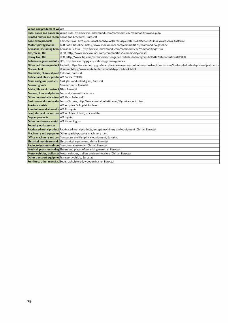
79
Wood and products of wood and cork (except furniture); articles of straw and plaiting materials (20)WB
Pulp, paper and paper products (21)Wood pulp, http://www.indexmundi.com/commodities/?commodity=wood-pulp
Printed matter and recorded media (22)Books and brochures, Eurostat
Coke oven products Chinese Coke, http://en.sxcoal.com/NewsDetail.aspx?cateID=170&id=83293&keyword=coke%20price
Motor spirit (gasoline) Gulf Coast Gasoline, http://www.indexmundi.com/commodities/?commodity=gasoline
Kerosene, including kerosene type jet fuelKerosene Jet fuel, http://www.indexmundi.com/commodities/?commodity=jet-fuel
Gas/Diesel Oil ULSD, http://www.indexmundi.com/commodities/?commodity=diesel
Heavy Fuel Oil HFO, http://www.bp.com/extendedsectiongenericarticle.do?categoryId=9041229&contentId=7075080
Petroleum gases and other gaseous hydrocarbons, except natural gasLPG, http://www.mylpg.eu/stations/germany/prices
Other petroleum productsAsphalt, https://www.dot.ny.gov/main/business-center/contractors/construction-division/fuel-asphalt-steel-price-adjustments
Nuclear fuel Uranium,http://www.metalbulletin.com/My-price-book.html
Chemicals, chemical products and man-made fibres (24)Chlorine, Eurostat
Rubber and plastic products (25)WB Rubber TSR20
Glass and glass products Cast glass and rolled glass, Eurostat
Ceramic goods Ceramic parts, Eurostat
Bricks, tiles and construction products, in baked clayTiles, Eurostat
Cement, lime and plaster Eurostat, cement trade data
Other non-metallic mineral productsWB Phosphate rock
Basic iron and steel and of ferro-alloys and first products thereofFerro-Chrome, http://www.metalbulletin.com/My-price-book.html
Precious metals WB av. price Gold,plat & silver
Aluminium and aluminium productsWB Al. Ingots
Lead, zinc and tin and products thereofWB av. Price of lead, zinc and tin
Copper products WB ingots
Other non-ferrous metal productsWB Nickel Ingots
Foundry work services
Fabricated metal products, except machinery and equipment (28)Fabricated metal products, except machinery and equipment (China), Eurostat
Machinery and equipment n.e.c. (29)Other special-purpose machinery n.e.c
Office machinery and computers (30)Computers and Periphical equipment, Eurostat
Electrical machinery and apparatus n.e.c. (31)Electronical equipment, china, Eurostat
Radio, television and communication equipment and apparatus (32)Consumer electronics(China(, Eurostat
Medical, precision and optical instruments, watches and clocks (33)Sheets and plates of polarising material, Eurostat
Motor vehicles, trailers and semi-trailers (34)Motor vehicles, trailers and semi-trailers (China), Eurostat
Other transport equipment (35)Transport vehicle, Eurostat
Furniture; other manufactured goods n.e.c. (36)Seats, upholstered, wooden frame, Eurostat

80
Table 26 G-matrix, Vessel transport Correspondence matrix
Sector/Activity Large Dry BulkDry Bulk General Cargo Container Reefer Crude Oil RoRo Chemical Oil Products LNG LPG
Paddy rice 0 1 0 0 0 0 0 0 0 0 0
Wheat 0 1 0 0 0 0 0 0 0 0 0
Cereal grains nec 0 1 0 0 0 0 0 0 0 0 0
Vegetables, fruit, nuts 0 0 0 0 1 0 0 0 0 0 0
Oil seeds 0 1 0 0 0 0 0 0 0 0 0
Sugar cane, sugar beet 0 0 0 1 0 0 0 0 0 0 0
Plant-based fibers 0 1 0 0 0 0 0 0 0 0 0
Crops nec 0 1 0 0 0 0 0 0 0 0 0
Cattle 0 0 0 0 1 0 0 0 0 0 0
Pigs 0 0 0 0 1 0 0 0 0 0 0
Poultry 0 0 0 0 1 0 0 0 0 0 0
Meat animals nec 0 0 0 0 1 0 0 0 0 0 0
Animal products nec 0 0 0 0 1 0 0 0 0 0 0
Raw milk 0 0 0 0 1 0 0 0 0 0 0
Wool, silk-worm cocoons 0 0 1 0 0 0 0 0 0 0 0
Products of forestry, logging and related services (02)0 0 0 1 0 0 0 0 0 0 0
Fish and other fishing products; services incidental of fishing (05)0 0 0 1 1 0 0 0 0 0 0
Coal and lignite; peat (10) 1 0 0 0 0 0 0 0 0 0 0
Crude petroleum and services related to crude oil extraction, excluding surveying0 0 0 0 0 1 0 0 0 0 0
Natural gas and services related to natural gas extraction, excluding surveying0 0 0 0 0 0 0 0 0 1 0
Other petroleum and gaseous materials0 0 0 0 0 0 0 0 1 0 1
Uranium and thorium ores (12) 0 1 0 0 0 0 0 0 0 0 0
Iron ores 1 0 0 0 0 0 0 0 0 0 0
Copper ores and concentrates 0 1 0 0 0 0 0 0 0 0 0
Nickel ores and concentrates 0 1 0 0 0 0 0 0 0 0 0
Aluminium ores and concentrates0 1 0 0 0 0 0 0 0 0 0
Precious metal ores and concentrates0 1 0 0 0 0 0 0 0 0 0
Lead, zinc and tin ores and concentrates0 1 0 0 0 0 0 0 0 0 0
Other non-ferrous metal ores and concentrates0 1 0 0 0 0 0 0 0 0 0
Stone 0 1 0 0 0 0 0 0 0 0 0
Sand and clay 0 1 0 0 0 0 0 0 0 0 0
Chemical and fertilizer minerals, salt and other mining and quarrying products n.e.c.0 1 0 0 0 0 0 0 0 0 0
Products of meat cattle 0 0 0 0 1 0 0 0 0 0 0
Products of meat pigs 0 0 0 0 1 0 0 0 0 0 0
Products of meat poultry 0 0 0 0 1 0 0 0 0 0 0
Meat products nec 0 0 0 0 1 0 0 0 0 0 0
Products of Vegetable oils and fats0 0 0 0 0 0 0 0 1 0 0
Dairy products 0 0 0 0 1 0 0 0 0 0 0
Processed rice 0 1 0 0 0 0 0 0 0 0 0
Sugar 0 1 0 0 0 0 0 0 0 0 0
Food products nec 0 0 0 0 1 0 0 0 0 0 0
Beverages 0 0 0 1 0 0 0 0 0 0 0
Fish products 0 0 0 0 1 0 0 0 0 0 0
Tobacco products (16) 0 0 0 1 0 0 0 0 0 0 0
Textiles (17) 0 0 0 1 0 0 0 0 0 0 0
Wearing apparel; furs (18) 0 0 0 1 0 0 0 0 0 0 0
Leather and leather products (19)0 0 0 1 0 0 0 0 0 0 0
Wood and products of wood and cork (except furniture); articles of straw and plaiting materials (20)0 0 1 0 0 0 0 0 0 0 0
Pulp, paper and paper products (21)0 0 1 0 0 0 0 0 0 0 0
Printed matter and recorded media (22)0 0 0 1 0 0 0 0 0 0 0
Coke oven products 0 1 0 0 0 0 0 0 0 0 0
Motor spirit (gasoline) 0 0 0 0 0 0 0 0 1 0 0
Kerosene, including kerosene type jet fuel0 0 0 0 0 0 0 0 1 0 0
Gas/Diesel Oil 0 0 0 0 0 0 0 0 1 0 0
Heavy Fuel Oil 0 0 0 0 0 0 0 0 1 0 0
Petroleum gases and other gaseous hydrocarbons, except natural gas0 0 0 0 0 0 0 0 0 0 0
Other petroleum products 0 0 0 0 0 0 0 0 1 0 0
Nuclear fuel 0 1 0 0 0 0 0 0 0 0 0
Chemicals, chemical products and man-made fibres (24)0 0 0 0 0 0 0 1 0 0 0
Rubber and plastic products (25) 0 0 0 1 0 0 0 0 0 0 0
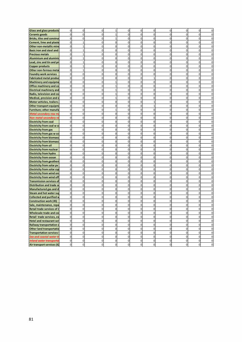
81
Glass and glass products 0 0 0 1 0 0 0 0 0 0 0
Ceramic goods 0 0 0 1 0 0 0 0 0 0 0
Bricks, tiles and construction products, in baked clay0 0 0 1 0 0 0 0 0 0 0
Cement, lime and plaster 0 1 0 0 0 0 0 0 0 0 0
Other non-metallic mineral products0 1 0 0 0 0 0 0 0 0 0
Basic iron and steel and of ferro-alloys and first products thereof0 1 0 0 0 0 0 0 0 0 0
Precious metals 0 1 0 0 0 0 0 0 0 0 0
Aluminium and aluminium products0 1 0 0 0 0 0 0 0 0 0
Lead, zinc and tin and products thereof0 1 0 0 0 0 0 0 0 0 0
Copper products 0 1 0 0 0 0 0 0 0 0 0
Other non-ferrous metal products0 1 0 0 0 0 0 0 0 0 0
Foundry work services 0 0 0 0 0 0 0 0 0 0 0
Fabricated metal products, except machinery and equipment (28)0 0 0 0 0 0 1 0 0 0 0
Machinery and equipment n.e.c. (29)0 0 0 1 0 0 0 0 0 0 0
Office machinery and computers (30)0 0 0 1 0 0 0 0 0 0 0
Electrical machinery and apparatus n.e.c. (31)0 0 0 1 0 0 0 0 0 0 0
Radio, television and communication equipment and apparatus (32)0 0 0 1 0 0 0 0 0 0 0
Medical, precision and optical instruments, watches and clocks (33)0 0 0 1 0 0 0 0 0 0 0
Motor vehicles, trailers and semi-trailers (34)0 0 0 0 0 0 1 0 0 0 0
Other transport equipment (35) 0 0 0 0 0 0 1 0 0 0 0
Furniture; other manufactured goods n.e.c. (36)0 0 0 1 0 0 0 0 0 0 0
Metal secondary raw materials 0 0 0 0 0 0 0 0 0 0 0
Non-metal secondary raw materials0 0 0 0 0 0 0 0 0 0 0
Electricity from coal 0 0 0 0 0 0 0 0 0 0 0
Electricity from coal w ccs 0 0 0 0 0 0 0 0 0 0 0
Electricity from gas 0 0 0 0 0 0 0 0 0 0 0
Electricity from gas w ccs 0 0 0 0 0 0 0 0 0 0 0
Electricity from biomass&waste 0 0 0 0 0 0 0 0 0 0 0
Electricity from biomass w ccs 0 0 0 0 0 0 0 0 0 0 0
Electricity from oil 0 0 0 0 0 0 0 0 0 0 0
Electricity from nuclear 0 0 0 0 0 0 0 0 0 0 0
Electricity from hydro 0 0 0 0 0 0 0 0 0 0 0
Electricity from ocean 0 0 0 0 0 0 0 0 0 0 0
Electricity from geothermal 0 0 0 0 0 0 0 0 0 0 0
Electricity from solar pv 0 0 0 0 0 0 0 0 0 0 0
Electricity from solar csp 0 0 0 0 0 0 0 0 0 0 0
Electricity from wind onshore 0 0 0 0 0 0 0 0 0 0 0
Electricity from wind offshore 0 0 0 0 0 0 0 0 0 0 0
Transmission services of electricity0 0 0 0 0 0 0 0 0 0 0
Distribution and trade services of electricity0 0 0 0 0 0 0 0 0 0 0
Manufactured gas and distribution services of gaseous fuels through mains0 0 0 0 0 0 0 0 0 0 0
Steam and hot water supply services0 0 0 0 0 0 0 0 0 0 0
Collected and purified water, distribution services of water (41)0 0 0 0 0 0 0 0 0 0 0
Construction work (45) 0 0 0 0 0 0 0 0 0 0 0
Sale, maintenance, repair of motor vehicles, motor vehicles parts, motorcycles, motor cycles parts and accessoiries0 0 0 0 0 0 0 0 0 0 0
Retail trade services of motor fuel0 0 0 0 0 0 0 0 0 0 0
Wholesale trade and commission trade services, except of motor vehicles and motorcycles (51)0 0 0 0 0 0 0 0 0 0 0
Retail trade services, except of motor vehicles and motorcycles; repair services of personal and household goods (52)0 0 0 0 0 0 0 0 0 0 0
Hotel and restaurant services (55)0 0 0 0 0 0 0 0 0 0 0
Railway transportation services 0 0 0 0 0 0 0 0 0 0 0
Other land transportation services0 0 0 0 0 0 0 0 0 0 0
Transportation services via pipelines0 0 0 0 0 0 0 0 0 0 0
Sea and coastal water transportation services0 0 0 0 0 0 0 0 0 0 0
Inland water transportation services0 0 0 0 0 0 0 0 0 0 0
Air transport services (62) 0 0 0 0 0 0 0 0 0 0 0

82
Supporting and auxiliary transport services; travel agency services (63)0 0 0 0 0 0 0 0 0 0 0
Post and telecommunication services (64)0 0 0 0 0 0 0 0 0 0 0
Financial intermediation services, except insurance and pension funding services (65)0 0 0 0 0 0 0 0 0 0 0
Insurance and pension funding services, except compulsory social security services (66)0 0 0 0 0 0 0 0 0 0 0
Services auxiliary to financial intermediation (67)0 0 0 0 0 0 0 0 0 0 0
Real estate services (70) 0 0 0 0 0 0 0 0 0 0 0
Renting services of machinery and equipment without operator and of personal and household goods (71)0 0 0 0 0 0 0 0 0 0 0
Computer and related services (72)0 0 0 0 0 0 0 0 0 0 0
Research and development services (73)0 0 0 0 0 0 0 0 0 0 0
Other business services (74) 0 0 0 0 0 0 0 0 0 0 0
Public administration and defence services; compulsory social security services (75)0 0 0 0 0 0 0 0 0 0 0
Education services (80) 0 0 0 0 0 0 0 0 0 0 0
Health and social work services (85)0 0 0 0 0 0 0 0 0 0 0
Collection and treatment services of sewage0 0 0 0 0 0 0 0 0 0 0
Collection of waste 0 0 0 0 0 0 0 0 0 0 0
Incineration of waste 0 0 0 0 0 0 0 0 0 0 0
Landfill of waste 0 0 0 0 0 0 0 0 0 0 0
Sanitation, remediation and similar services0 0 0 0 0 0 0 0 0 0 0
Membership organisation services n.e.c. (91)0 0 0 0 0 0 0 0 0 0 0
Recreational, cultural and sporting services (92)0 0 0 0 0 0 0 0 0 0 0
Other services (93) 0 0 0 0 0 0 0 0 0 0 0
Private households with employed persons (95)0 0 0 0 0 0 0 0 0 0 0
Extra-territorial organizations and bodies0 0 0 0 0 0 0 0 0 0 0