Improving the Accuracy of Economic Measurement
with Multiple Data Sources:
The Case of Payroll Employment Data
Tomaz Cajner Leland D. Crane Ryan A. Decker
Adrian Hamins-Puertolas Christopher Kurz∗
December 18, 2020
Abstract
This paper combines information from two sources of U.S. private payroll employment to increase
the accuracy of real-time measurement of the labor market. The sources are the Current Employment
Statistics (CES) from BLS and microdata from the payroll processing firm ADP. We briefly describe
the ADP-derived data series, compare it to the BLS data, and describe an exercise that benchmarks
the data series to an employment census. The CES and the ADP employment data are each derived
from roughly equal-sized samples. We argue that combining CES and ADP data series reduces the
measurement error inherent in both data sources. In particular, we infer “true” unobserved payroll
employment growth using a state-space model and find that the optimal predictor of the unobserved
state puts approximately equal weight on the CES and ADP-derived series. Moreover, the estimated
state contains information about future readings of payroll employment.
Keywords: labor market, economic measurement, big data, state-space models.
JEL Classification: J2, J11, C53, C55, C81.
∗All authors are at the Federal Reserve Board of Governors. We thank ADP for access to and help with thepayroll microdata that underlie the work described by this paper. In particular, this work would not have beenpossible without the support of Jan Siegmund, Ahu Yildirmaz, and Sinem Buber. We are grateful for discussionswith Katharine Abraham, Boragan Aruoba, Simon Freyaldenhoven, Erik Hurst, Gray Kimbrough, Alan Krueger,Norman Morin, Matthew Shapiro, John Stevens, David Wilcox, Mark Zandi, and seminar participants at the FederalReserve Board, the Federal Reserve Bank of Cleveland, ESCoE Conference on Economic Measurement, BLS, NBERCRIW meetings, the Bank of England, and the 2018 ASSA meetings. The analysis and conclusions set forth hereare those of the authors and do not indicate concurrence by other members of the research staff or the Board ofGovernors.

1 Introduction
Economists and statisticians are increasingly confronted with new data sources, often produced
by private companies as part of their business operations, that may be useful for economic re-
search and measurement. These new data hold promise for advancing economic measurement
and understanding, but their use raises many questions. How are new, alternative data differ-
ent from traditional surveys and censuses? How are we to assess their reliability? How should
multiple disparate data sources be synthesized to produce the best possible estimates?
We seek to answer these questions in the context of measuring payroll employment. In
particular, we use data from a private payroll provider—ADP—to build an index of U.S. private
payroll employment, similar in spirit to the Current Employment Statistics (CES) survey. While
the CES survey is carefully conducted and uses an extremely large sample, it still suffers from
significant sampling error and nonresponse issues. The ADP-derived employment indexes are
based on a sample that is roughly the same size as the CES sample, so it is plausible that pooling
the information from ADP with that from CES would reduce sampling error and increase our
understanding of the state of the labor market at a given time.
Previous work by Cajner et al. (2018) describes the construction of weekly and monthly ag-
gregate employment series based on ADP’s weekly payroll microdata. Their aggregate series
(referred to as ADP-FRB) are designed to be an independent signal about labor market con-
ditions rather than solely an attempt to forecast monthly BLS employment figures. However,
Cajner et al. (2018) do indeed find that the timeliness and frequency of the ADP payroll micro-
data improves forecast accuracy for both current-month employment and revisions to the BLS
CES data.
In this paper we further compare the ADP-FRB index to existing, high-quality government
estimates and find encouraging results. The ADP-FRB index, and state-space estimates derived
from it, provide information about future CES estimates in real time, including at the start of
the Great Recession. In addition, we integrate benchmark employment data and compare the
ADP-FRB benchmark revisions with the CES benchmark revisions. While the CES and ADP-
FRB series are both prone to significant sampling and non-sampling error, the BLS Quarterly
Census of Employment and Wages (QCEW) is generally considered the “final word” for annual
1

employment growth because of its comprehensive administrative source data. Consequently,
we benchmark the ADP-based series to the QCEW on an annual basis. The benchmarking
procedure is similar to CES benchmarking and ensures that year-to-year changes in ADP-FRB
are governed by the QCEW, while higher-frequency changes, and the period after the most
recent benchmark, are mostly a function of the ADP data.1
Existing work on using nontraditional data sources for economic measurement typically
takes official government data as the source of truth, at all frequencies. For example, the
monthly National Employment Report (ADP-NER) series published by ADP are constructed
with the goal of predicting the fully revised CES data.2 In this paper we take a different ap-
proach by recognizing that both CES and ADP-FRB employment are subject to non-negligible
measurement error and by using the Kalman filter to extract estimates of unobserved “true”
employment growth from observations of both series.
Our baseline model assumes that true U.S. employment growth follows a persistent, latent
process and that both the CES and ADP-FRB estimates are noisy signals of this underlying
process. Standard state-space tools allow us to estimate the latent process and the observation
error associated with each series. We find that the optimal predictor of the unobserved state,
using only contemporaneous information, puts approximately equal weight on the CES and
ADP-FRB series. This finding is not necessarily surprising, as the ADP sample covers roughly
similar fraction of private nonfarm U.S. employment as the CES sample, so the sampling errors
ought to be of roughly similar magnitudes. We also show that the smoothed state estimate, as
constructed in real time, helps forecast future values of CES. Throughout, we focus on the role
of these privately generated data as a complement to existing official statistics. While there is
no substitute for official statistics in terms of consistency, transparency, and scientific collection
methods, official numbers do have limitations that alternative data sources can address.
The paper proceeds as follows. Section 2 reviews the related literature. Section 3 describes
the process of creating ADP-based employment indexes and lays out the strengths and the in-
herent limitations of measuring nationwide payroll employment with ADP data. In section 4
1Benchmarking illustrates an essential role that government statistics play even when there is significant valuein nontraditional data sources.
2Mastercard’s SpendingPulse, which attempts to forecast U.S. retail sales, is another example.
2
we compare the annual ADP-FRB employment estimates to the official benchmarks, discuss
the role of the birth-death model in the official estimates, present a case study of the useful-
ness of alternative employment data during the Great Recession, and show the efficacy of the
ADP-FRB estimates in predicting fully revised CES payroll employment numbers. Section 5
introduces the state-space model that combines the information from both the ADP-FRB and
CES-based estimates and provides evidence that the combined state improves our understand-
ing of current and future payroll gains. Section 6 concludes.
2 Related Literature
Ours is not the first paper to make use of ADP payroll data. Several papers study the National
Employment Report (NER), ADP’s publicly available monthly estimate of U.S. payroll gains
constructed jointly with Moody’s Analytics. Importantly, NER estimates are derived from a
model including not only ADP microdata but also other contemporaneous and lagged indica-
tors of U.S. economic activity. The existing literature finds that the NER moves closely with
CES (Phillips and Slijk, 2015) and has some ability to forecast CES, though it does not appear
to improve forecasts based on other available information, such as existing consensus forecasts
(Gregory and Zhu, 2014; Hatzius et al., 2016).
As noted above, we do not use the NER but instead focus on the ADP microdata. A num-
ber of recent papers explore these data. Cajner et al. (2018) analyze the representativeness of
ADP microdata (relative to CES and QCEW) and construct an ADP payroll index that can im-
prove forecasts of CES; we employ that index in the present paper. Ozimek, DeAntonio and
Zandi (2017) use ADP’s linked employer-employee microdata to study the negative effect of
workforce aging on aggregate productivity growth. Grigsby, Hurst and Yildirmaz (fortcom-
ing) study wage rigidity in the same data, finding that the high-frequency microdata can be
useful for shedding light on a key business cycle question. Cho (2018) uses ADP microdata to
study the employment and wage effects of the 2009 American Recovery and Reinvestment Act.
Our approach in the present paper is different from those above in that we explicitly inves-
tigate the usefulness of ADP as a supplement to CES data for tracking the underlying state of
3

the labor market. In this respect, our work is inspired by Aruoba et al. (2016) who note difficul-
ties in assessing the growth of aggregate output in real time given limitations on the compre-
hensiveness and timeliness of GDP measures. Two independent measures of GDP exist—the
commonly reported expenditure-side approach and the income-based approach—and both are
prone to measurement errors arising from various sources. Aruoba et al. (2016) combine the
two measures using a state-space framework, recovering an underlying state of output growth
which they label “gross domestic output”. We follow this general approach with a focus on
employment rather than output.
3 Data
This paper primarily uses three data sources: ADP microdata, the Current Employment Statis-
tics (CES) survey, and the Quarterly Census of Employment and Wages (QCEW). Before turn-
ing to the ADP microdata in Section 3.1, it is useful to briefly lay out the relevant features of the
CES and the QCEW.
The CES is the main source of monthly employment information in the United States. It is
published by BLS a few days after each reference month and is based on a stratified-sample sur-
vey, which includes about 500,000 private establishments covering about 24 percent of all U.S.
private employees.3 However, the CES survey response rate—the share of eligible units that
respond by the final reading—is only about 60 percent, which implies that CES data contain in-
formation for about 15 percent of U.S. private employment.4 The CES asks each respondent for
the count of employees who worked or received pay for any part of the pay period including
the 12th of the reference month. Aggregate CES employment growth is a (weighted) average of
the growth reported by units that respond for two or more consecutive months, plus a residual
adjustment for establishment birth and death.
While the CES is a very large survey, it is still based on a sample and subject to sampling
and non-sampling error (as discussed further below). In contrast, the QCEW, also maintained
3See BLS (2019). Note that the CES contains data for total nonfarm payroll employment, but here we focus onlyon private payroll employment, excluding government employment to be consistent with the reliable scope of ADP.
4For CES response rates, see: https://www.bls.gov/osmr/response-rates/.
4

by BLS, is a near-census of employment covered by unemployment insurance and serves as the
sampling frame for much of the CES as well as the target for the annual benchmark of the CES.
The employment concept for the QCEW is the number of workers who worked or received
pay for any part of the pay period including the 12th of the reference month (even though the
firm may have been paying UI insurance for other workers at other times during the month).
The main drawback of the QCEW is that the data are collected quarterly and published with a
lag of two quarters. Thus, while the QCEW has negligible sampling error, it is of limited use to
real-time decision makers. In addition, the QCEW is subject to various sources of non-sampling
error.5 Nevertheless, we follow CES in using the QCEW for reweighting the ADP microdata
and as a benchmark target.
3.1 Structure of the ADP Microdata
ADP provides human capital management services to firms, including payroll processing. Pro-
cessing payroll for a client firm involves many tasks, including maintaining worker records,
calculating taxes, and issuing paychecks. ADP processes payroll for about 26 million U.S.
workers each month (about 20 percent of total U.S. private employment). The structure of
the microdata is determined by the business needs of ADP. ADP maintains records at the level
of payroll account controls (PAC), which often correspond to business establishments (but may
sometimes correspond to firms) as defined by the Census Bureau and BLS. Each PAC updates
their records at the end of each pay period. The records consist of the date payroll was pro-
cessed, employment information for the pay period, and many time-invariant PAC characteris-
tics (such as an anonymized PAC identifier, NAICS industry code, zip code, etc.). PAC records
include both the number of individuals employed (“active employees”) and the number of
individuals issued a paycheck in a given pay period (“paid employees”). Active employees
include wage earners with no hours in the pay period, workers on unpaid leave, and the like.
Paid employees include any wage or salary workers issued regular paychecks during the pay
period as well as those issued bonus checks and payroll corrections. In this paper we focus ex-
clusively on active employment, having found that it is substantially less volatile, more closely
5For a detailed analysis of measurement challenges in CES and QCEW, see Groen (2012).
5

resembles officially published aggregates, and performs better in forecasting exercises, though
we plan to further investigate the active/paid distinction in the future.6
The data begin in July 1999.7 In terms of frequency, the files we use are weekly snapshots
of individual PAC records, taken every Saturday since July 2009 (snapshots were taken semi-
monthly between May 2006 and June 2009 and monthly before May 2006). Each snapshot
contains the most recent pay date for each PAC, the relevant employment counts, and the other
information described above. As few firms regularly process payroll more than once per week,
the weekly snapshots provide a comprehensive history of PAC-level employment dynamics.8
We can compare ADP payroll microdata to the QCEW and CES data in terms of pay fre-
quency, region, establishment size, and industry composition. Most notably, ADP has sig-
nificantly more employment in mid-sized units than does CES, with a distribution that looks
reasonably similar to QCEW.9
3.2 Series Construction
The process of transforming the raw data to usable aggregate series is complex. Here we pro-
vide a brief, simplified explanation of the process. The interested reader may refer to Cajner
et al. (2018) for details.
Each week, we calculate the weighted average growth of employment at PACs appearing in
the data for two consecutive weeks. The restriction to “continuers” allows us to abstract from
changes in the size of ADP’s client base. For example, if ADP suddenly gains a large number
of clients this expansion does not directly affect our estimated level of employment. Rather, the
growth rate of the businesses once they enter the sample is what matters. As long as business
growth is independent of entering or exiting the ADP sample, the growth rate of continuers
6One topic for further investigation is exactly why active employment performs better than paid employment.It is possible that double counting due to the inclusion of payroll corrections, reimbursements, and bonuses addsnoise to paid employment as measured in the ADP data. See Cajner et al. (2018) for further discussion.
7When accessing the microdata, we follow a number of procedures to ensure confidentiality. Business names arenot present in the data we access.
8While ADP microdata generally do not revise over time, our employment indexes do revise in a way analogousto CES data. First, our real-time readings for a particular month revise as we incorporate information for additionalweeks and business that pay at lower pay frequency. Second, we revise our data annually by benchmarking it toQCEW.
9For more detail, see Cajner et al. (2018).
6

will be a valid estimate of aggregate growth (of continuers).10
Growth rates are weighted by PAC employment and further weighted for representative-
ness by size and industry. We use QCEW employment counts by establishment size and two-
digit NAICS as the target population. Formally, let wj,t be the ratio of QCEW employment in a
size-industry cell j to ADP employment in cell j in week t, let C(j) be the set of ADP businesses
in cell j, let ei,t be the employment of the i’th business, and let gi,t =ei,t−ei,t−1
ei,t−1be the weekly
growth rate of business i.11 Aggregate growth is estimated as:
gt =∑J
j=1 wj,t−1 ∑i∈C(j) ei,t−1gi,t
∑Jj=1 wj,t−1 ∑i∈C(j) ei,t−1
. (1)
Cumulating the weekly growth rates across time yields a weekly index level for employ-
ment. Our focus in this paper is on monthly estimates. We calculate the monthly index as the
average of the weekly index for each month, weighting by days to account for partial weeks
in each month.12 Monthly averaging smooths through the weekly volatility, and the results
in Cajner et al. (2018) suggest that averaging improves performance relative to point-in-time
methods more similar to the CES. The monthly index is seasonally adjusted at the aggregate
level using the X-12 algorithm.13
Figure 1 displays the seasonally adjusted ADP-FRB series (black thick line) along with the
indexed CES estimate (gray thin line). Importantly, the growth rate of the (weighted) ADP-
FRB series is very similar to the CES, and the business-cycle frequency fluctuations are very
closely aligned. Moreover, this ADP-FRB series does not incorporate any of the benchmarking
discussed below, so nothing forces it to resemble CES. It is also evident that the ADP-FRB
series is volatile, and much of the month-to-month variation does not appear to be related to
10This assumption will inevitably be violated in practice, as firms that are growing fast or shrinking quickly willmake different operational choices with respect to their payroll systems. However, we are not aware of any clearevidence on the direction of these biases or any indication that their magnitudes are economically significant.
11For weighting, we use March QCEW employment values for each year. For years where the March QCEW hasnot been released, we use the last available March QCEW. While we could allow QCEW values to vary quarterly ormonthly, the shares are slow moving and thus this change would not significantly alter the results.
12For example, if a calendar week has four days in January and three days in February, our weighting by daysprocedure proportionally attributes the weekly employment to both months.
13BLS seasonally adjusts the CES data with X-13ARIMA-SEATS at the 3-digit NAICS level and then aggregatesthose seasonally adjusted series.
7

the monthly swings in the CES data. We interpret this finding as evidence that both series
are contaminated with measurement error, which can plausibly be attenuated by modeling the
series jointly. For reference, Figure 1 also shows the ADP-FRB unweighted series, which does
not correct the ADP size-industry distribution. Clearly, the unweighted series has a markedly
different trend growth rate, though it shares the qualitative business-cycle frequency behavior
of the others.14
Monthly Growth Rates
Jan2000 Jan2005 Jan2010 Jan2015 Jan2020-1
-0.5
0
0.5
1
Pe
rce
nt
Ch
an
ge
CES Private Employment
ADP-FRB
ADP-FRB Unweighted
Indexed Levels
Jan2000 Jan2005 Jan2010 Jan2015 Jan202080
90
100
110
120
130
140
CES Private Employment
ADP-FRB
ADP-FRB Unweighted
Note: Monthly data (current vintage), normalized to 100 in 2010.Source: ADP, CES, authors’ calculations. CES series is benchmarked; ADP-FRB is not.
Figure 1: Monthly Growth Rates and Indexed Levels
3.3 Strengths and Weaknesses of Different Types of Payroll Employment Data
Perhaps the most important issue when analyzing the quality of a dataset is its representa-
tiveness. Obviously, the QCEW data have a clear advantage here because these data represent
14While we do not directly use the weekly ADP-FRB series in this paper, we view these high-frequency measure-ments as a promising topic for future research on, for example, natural disasters. The weekly series are discussedin more detail in Cajner et al. (2018).
8

population counts.15 In contrast, CES and ADP estimates are sample based. As with CES, our
ADP samples are adjusted with weights that are meant to make the estimates representative of
the United States, but the weighting does not solve all issues. In the case of ADP, an important
sample selection issue exists because only the firms that hire ADP to manage their payrolls
show up in the ADP data. In the case of CES, the data are based on a probability sample of
establishments, but because the response rates are only about 60 percent as argued above, this
can introduce a potential sample selection issue as well (Kratzke, 2013).
Both the ADP and the CES data are subject to dynamic selection issues related to establish-
ment entry and exit. In the United States, young firms account for a disproportionate share of
employment growth (Haltiwanger, Jarmin and Miranda, 2013); indeed, mean and median net
employment growth rates of firms above age five tend to be around zero (Decker et al., 2014).
A critical limitation of the CES sample is its lack of coverage of new firms and establishments.16
In addition, the CES does not directly measure establishment deaths. BLS attempts to correct
for these shortcomings using an establishment birth/death estimation methodology; for most
of the time period we study (up to early 2020), this estimation involved a two-step approach.
In the first step, employment losses from known business deaths are excluded from the sample
to offset the missing employment gains from new business births. Thus, dead establishments
(i.e., those reporting zero employment) and nonrespondents (suspected dead establishments)
are implicitly given the same growth rate as the continuing establishments in the CES survey
under the assumption that employment at establishment births exceeds employment at estab-
lishment deaths by an amount equal to the growth of continuing establishments. In the second
step, an ARIMA model based on historical QCEW data estimates the birth/death residual:
employment at newly formed establishments less employment at exiting establishments. This
estimate is added to the estimates from the CES establishment sample to generate the final
CES estimate. In many months, the model’s contribution to headline employment estimates
is sizable.17 For example, since 2009 the net birth-death adjustment has added a nontrivial
15Note, though, that there is a small scope discrepancy between QCEW on the one hand and CES/ADP on theother hand: about 3 percent of jobs that are within scope for CES/ADP estimates are exempt from UI tax law. Formore detail, see https://www.bls.gov/news.release/cewqtr.tn.htm.
16The CES sample is redrawn only once a year (BLS, 2019).17See a discussion of the model and its recent contributions here: https://www.bls.gov/web/empsit/cesbd.htm.
9

average of 800,000 jobs to a particular year’s employment gains, or roughly 40 percent. Ac-
tual new firms do not affect CES monthly estimates until the sample is rotated (though births
will be captured at an annual frequency when annual benchmarks are released, as we describe
below).18
Even after an annual benchmark revision, the monthly CES data never truly account for the
birth and death of establishments. When a benchmark revision occurs, with the January CES
release each year, the previous year’s March level of the CES data is set to the March level
of QCEW employment. The monthly sample-based estimates for the 11 months preceding
the March benchmark are revised with a “wedge-back” procedure, where a linear fraction of
the benchmark revision is added to the CES level each month (BLS, 2019). The wedging-back
procedure results in a constant being added to the monthly change in employment each year.
So, while the year-to-year change in the post-benchmark CES data will capture the within-
QCEW-scope dynamics of entry and exit at the annual frequency, the monthly numbers will
never reflect the true monthly pattern of employment.
ADP data are subject to a related limitation in that we do not know the age composition
of ADP clients, nor do we observe firm or establishment age in the ADP microdata. However,
new and young firms may enter the ADP data immediately upon engaging ADP for payroll
services. While the number of young firms in ADP data is unknown, any number could be a
useful supplement to the CES data, in which young firms are absent until the sample rotation.
As discussed above, the ADP data consist of weekly snapshots (since July 2009). In contrast,
the QCEW and CES data contain information for only the pay period that includes the 12th day
of the month. As a result, the CES and QCEW data cannot measure employment activity over
the entire month, which can be especially problematic in the case of temporary distorting events
Importantly, this method was tweaked—possibly temporarily—early in the COVID-19 pandemic period to allow forestablishment shutdown and nonresponse to affect death estimates more materially and to allow current continuers’growth patterns to affect estimates of the birth/death residual.
18The sampling frame is based on QCEW source data (state unemployment insurance (UI) records), which lagseveral months. It might be wondered if the UI records pick up new establishments quickly; this is apparently thecase. Employers must file UI taxes if they have paid (cumulatively) $1,500 or more in payroll, so most new em-ployers would appear in the UI records very quickly; see https://oui.doleta.gov/unemploy/pdf/uilawcompar/2018/coverage.pdf. However, note that even after a business birth appears in the UI records, there is also timerequired for sampling, contacting, and soliciting cooperation from the firm as well as verifying the initial data pro-vided. In practice, CES cannot sample and begin to collect data from new firms until they are at least a year old(BLS, 2019).
10
during the reference period. For example, an unusually large weather event (e.g., a hurricane
or a snow storm) that reduced employment during the reference period but left the rest of the
month unaffected would result in a CES employment report that understates the strength of
the labor market throughout the month. In the weekly ADP data we can, in principle, observe
both the shock and the recovery. In any case, averaging the level of employment for the month
attenuates the impact of such short-lived events.
Finally, the QCEW and ADP data are both essentially administrative data and thus arguably
somewhat less prone to reporting errors and nonresponse, which are often significant problems
survey data such as the CES.
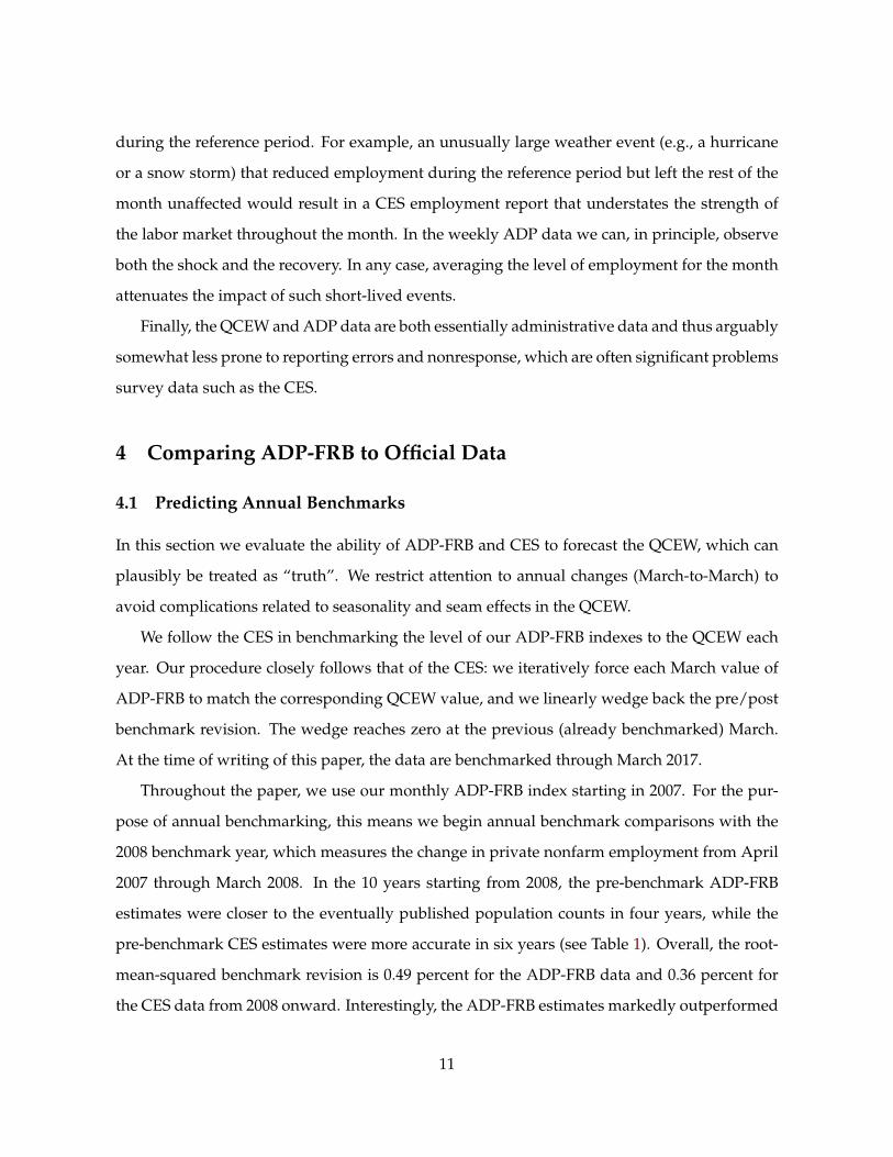
4 Comparing ADP-FRB to Official Data
4.1 Predicting Annual Benchmarks
In this section we evaluate the ability of ADP-FRB and CES to forecast the QCEW, which can
plausibly be treated as “truth”. We restrict attention to annual changes (March-to-March) to
avoid complications related to seasonality and seam effects in the QCEW.
We follow the CES in benchmarking the level of our ADP-FRB indexes to the QCEW each
year. Our procedure closely follows that of the CES: we iteratively force each March value of
ADP-FRB to match the corresponding QCEW value, and we linearly wedge back the pre/post
benchmark revision. The wedge reaches zero at the previous (already benchmarked) March.
At the time of writing of this paper, the data are benchmarked through March 2017.
Throughout the paper, we use our monthly ADP-FRB index starting in 2007. For the pur-
pose of annual benchmarking, this means we begin annual benchmark comparisons with the
2008 benchmark year, which measures the change in private nonfarm employment from April
2007 through March 2008. In the 10 years starting from 2008, the pre-benchmark ADP-FRB
estimates were closer to the eventually published population counts in four years, while the
pre-benchmark CES estimates were more accurate in six years (see Table 1). Overall, the root-
mean-squared benchmark revision is 0.49 percent for the ADP-FRB data and 0.36 percent for
the CES data from 2008 onward. Interestingly, the ADP-FRB estimates markedly outperformed
11

the CES estimates during the Great Recession (2008-2010). Specifically, from 2008 to 2010 the
ADP-FRB absolute revisions averaged 200,000 per year, whereas the BLS-CES absolute revi-
sions averaged 490,000 per year. In contrast, between 2013-2017the pre-benchmark ADP-FRB
estimates consistently overpredicted employment growth.
An evaluation of the CES benchmark misses should also take the net birth-death model
into account, as the net birth-death adjustment adds roughly 40 percent to a particular year’s
employment change. As a result, a comparison of the benchmark misses of ADP-FRB series to
the CES data is not exactly direct, as the ADP-FRB data would likely only capture a portion of
the contribution of the employment contribution of births. The third row in Table 1 presents
the benchmark miss of the CES data without the inclusion of the net birth-death adjustment.
That is, the “CES no BD” row reflects the growth to the level of employment solely due to the
sample of businesses for which the CES data is collected.19
As can be seen in the table, the benchmark misses for CES excluding the net birth-death
adjustment are substantially larger (with a root-mean-squared revision of 0.65 percent on av-
erage since 2008). Since 2008, the misses have also been almost always positive, reflecting a
positive effect of establishments’ births on the level of employment. The negative revisions in
2009 and 2010 point toward the autoregressive nature of the birth-death adjustment carrying
inertia forward from previous years’ employment changes. That is, because new business for-
mation falls in recessionary years, the net effect of the birth-death framework overpredicts the
actual birth-death contribution to employment growth, and thus CES benchmark misses were
larger than benchmark misses of CES data with no birth-death adjustment.
We more formally test the performance of ADP-FRB and CES in predicting annual bench-
marked employment growth by running the following regressions. The dependent variable
is the annual change in employment from March of year t − 1 to March of year t as known
upon the release of the CES benchmark revision in February of year t + 1. We consider three
different independent variables, with each annual observation specified as the econometrician
19Even this comparison is not exactly direct since, as noted above, ADP data may capture some birth and death.Note that for our formal ADP-FRB series, we apply a “forward benchmark” procedure that is a rough versionof a birth-death model for adjusting sample-based estimates to account for biases resulting from birth, death, orother issues; this approach is similar to the bias adjustment method used by BLS prior to the introduction of thebirth/death model.
12

2008 2009 2010 2011 2012 2013 2014 2015 2016 2017ADP-FRB -173 -451 12 709 283 -230 -1030 -853 -322 -623CES -137 -933 -391 229 481 340 105 -259 -151 136CES No BD 645 -216 -55 561 972 975 874 638 737 1066
Notes: Units: Thousands of jobs. CES revisions are the post-benchmark (QCEW-based) March esti-mate less the pre-benchmark estimate. ADP-FRB revisions are calculated analogously. CES no BDare the CES benchmark revisions that would have occurred excluding net birth-death adjustment.Source: https://www.bls.gov/web/empsit/cesbmart.pdf, authors’ calculations.
Table 1: Level Differences between Private Employment Benchmarks and Estimates
observed them at the time of the CES jobs report for March of year t: (1) annual employment
change from March of t − 1 to March of t as estimated by monthly CES data; (2) estimated
annual employment change from March of t − 1 to March of t as estimated by monthly CES
data in which the contributions of the birth-death model have been removed; and (3) annual
employment change from March of t− 1 to March of t as observed in the ADP-FRB (“active”)
employment index.20 The purpose of the exercise is to evaluate the ability of an analyst to es-
timate “true” (i.e., benchmarked) employment gains for the past year, observed at the time of
the CES March employment report (in early April). At that time, the analyst has in hand CES
data for the first release of March of year t (which includes the second release of February of
year t and the third release of January of year t and all prior months). The analyst also has in
hand the past year’s ADP-FRB data up through the third week of March of year t. That is, we
estimate the following:
∆EMPBt = α + β∆EMPMarch
t + εt,
where ∆EMPt is the change in private nonfarm employment from March of year t− 1 to March
of t, the B superscript indicates the benchmark revision vintage of the series, the March su-
perscript indicates the vintage of the series that is released with the March jobs report in year
t (where we construct the annual estimate by summing all non-seasonally-adjusted monthly
estimates through the year), and ∆EMPMarcht can be the March vintage of CES, CES without
birth-death model contributions, or ADP-FRB (“active”) employment.
Table 2 reports results from this annual forecasting exercise. While we believe there is value
in reporting this formal test, given the extremely small sample size the results are suggestive
20We use non-seasonally-adjusted data for all variables used.
13

(1) (2) (3) (4) (5)CES 1.126*** 1.104***
(0.0316) (0.142)CES excluding Birth-Death 1.154*** 0.927***
(0.0235) (0.0847)ADP-FRB 0.976*** 0.0197 0.199**
(0.0543) (0.121) (0.0818)Constant -163.7* 604.5*** -135.1 -163.6* 452.5***
(76.93) (75.29) (172.8) (82.61) (79.37)RMSE 299.2 243.3 535.9 319.7 224.2
Notes: Dependent variable is benchmarked annual change in private nonfarm employment,March to March. Years 2008-2017. *, **, and *** indicate statistical significance at the 10%,5%, and 1% levels, respectively. Robust standard errors in parentheses.
Table 2: Forecasting Annual Employment Changes
at best and should be treated with caution. That said, we find that the best predictor of bench-
marked employment growth, according to both adjusted R2 and RMSE, is the CES series that
excludes birth-death model contributions (column 2). That is, the birth-death model does not
appear to improve estimates of annual employment growth beyond the inclusion of a simple
regression constant (compare columns 1 and 2). The ADP-FRB series (column 3) has predictive
content but is outperformed by both CES series. However, we do find that adding the ADP-
FRB series to the CES series that excludes birth-death contributions does improve forecasts
(column 5).21
While the regression results in Table 2 are interesting, it is difficult to draw conclusions from
such small-sample exercises. Moreover, ADP-FRB data are most valuable to policymakers if
they increase our ability to understand recessions in real time; the predictive power of ADP-
FRB during periods of steady, modest job growth is much less useful. We illustrate the point
with a simple case study from the only recession in our ADP sample.22
Consider the beginning of the Great Recession. The NBER business cycle dating committee
identified December 2007 as the business cycle peak, but throughout 2008, economic data sent
somewhat mixed signals about the deterioration of labor market conditions. CES data releases
from throughout 2008 were revised substantially with the 2009 QCEW benchmark.
The left panel of Figure 2 reports real time CES estimates along with the final (current vin-
21In unreported exercises, we find that the results are highly sensitive to the specific time period included.22ADP began taking snapshots on a semimonthly basis starting in May 2006.
14

Jul2007 Oct2007 Jan2008 Apr2008 Jul2008 Oct2008114600
114800
115000
115200
115400
115600
115800
116000
116200
Le
ve
l, T
ho
usan
ds o
f Job
s
ADP-FRB, real time
CES, final
Jul2007 Oct2007 Jan2008 Apr2008 Jul2008 Oct2008114600
114800
115000
115200
115400
115600
115800
116000
116200
Le
ve
l, T
ho
usan
ds o
f Job
s
CES, real time
CES, final
Note: Monthly data. NBER recession is shaded in gray. Real-time lines show each successive vintage as a connectedline, with the end point at the first-print value for that month. All series have been normalized to match the currentvintage CES estimate in August 2007.Source: ADP, CES, authors’ calculations.
Figure 2: Real-Time vs. Current Vintage Estimates
tage) CES estimate. The thick black line is the final CES estimate, which shows employment
losses of about 1.4 million jobs by August 2008. The dotted gray lines show each real-time
vintage CES estimate for 2008: each end point represents a first-print estimate, and the thicker
central line represents the estimate after a few monthly revisions (but before the benchmark
revision). That is, following the line back from an endpoint in month t, the line reflects the path
of employment as it would have been known to observers in month t (including revisions up
to that date). In the right panel, we show real-time estimates for the ADP-FRB index alongside
the final CES estimate for reference.23
As is apparent from Figure 2, in real time the ADP-FRB series was typically more accurate
in tracking the true pace of labor market deterioration during the first year of the recession.
By August, real-time CES estimates showed job losses totaling about 750,000, while ADP-FRB
was at approximately 1.0 million (both numbers should be compared with the current vintage
estimate of 1.4 million jobs lost). Better knowledge of this deterioration would have been useful
to policymakers as the critical fourth quarter of 2008 approached. In future cyclical downturns,
ADP data may again prove useful in previewing the eventual revisions to CES data.
23All of the real-time series have been normalized to equal the CES current vintage estimates in August 2008 toremove a level shift due to benchmark revisions.
15

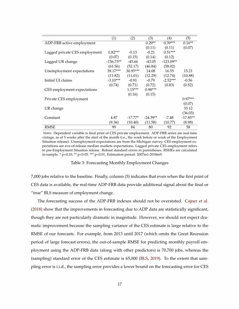
4.2 Predicting Monthly Employment
While annual forecasts of the benchmark revisions are important, the CES is a monthly mea-
sure of employment that revises over several releases as both more data and benchmarks be-
come available. In this section we evaluate the ability of the ADP-FRB employment indexes to
improve forecasts of CES data in real time and in conjunction with other real-time indicators.
Table 3 reports forecasting models described in Cajner et al. (2018) using real-time ADP indexes
and other variables to predict the final print of CES (i.e., after all of the revisions). In particular,
we estimated the following regression model:
∆EMPCES, f inalt = α + β1∆EMPADP-FRB,RT5
t + β2∆EMPCES,RTt−1 + βXt + ωt (2)
The explanatory variables include current-month real-time (five weeks after the start of the
month, which corresponds to the week before or the week of the Employment Situation re-
lease) ADP-FRB data, previous-month real-time (first print) CES private employment, as well
as initial unemployment insurance claims, Michigan Survey unemployment expectations, the
lagged (previous-month) unemployment rate change, and Bloomberg market CES payroll em-
ployment expectations. In addition, ωt = εt + ρεt−1 is an MA(1) error term.24
Cajner et al. (2018) discuss similar results in more detail; here we simply note that the ADP-
FRB indexes for active employment make statistically significant contributions to the model
and generate modest improvements to forecasting accuracy. Column (1) of Table 3 reports the
baseline forecasting model without the ADP-FRB data or market expectations. Adding market
expectations in column (2) improves the forecast notably, as can be seen from the 15,000-job
reduction in RMSE. In column (3) we add the ADP-FRB index and find that RMSE declines
and the ADP-FRB coefficient is statistically significant; that is, the inclusion of the ADP-FRB
index provides further marginal forecasting improvement beyond the inclusion of market ex-
pectations, in contrast to the Gregory and Zhu (2014) results using ADP-NER. In column (4) we
report a model including ADP-FRB but omitting market expectations, which reduces RMSE by
24The MA error term corrects for serial correlation in the errors when estimating equations of the change inemployment. The results for a similar specification using OLS are qualitatively similar, despite the existence ofserial correlation.
16
(1) (2) (3) (4) (5)ADP-FRB active employment 0.29** 0.39*** 0.16**
(0.11) (0.11) (0.07)Lagged private CES employment 0.82*** -0.13 -0.21 0.51***
(0.07) (0.15) (0.14) (0.12)Lagged UR change -156.73** -45.66 -43.05 -123.09**
(61.56) (52.17) (46.84) (58.02)Unemployment expectations 39.17*** 30.95*** 14.08 16.55 15.21
(11.82) (11.01) (12.29) (12.74) (10.88)Initial UI claims -3.10*** -0.91 -0.79 -2.52*** -0.56
(0.74) (0.71) (0.72) (0.83) (0.52)CES employment expectations 1.15*** 0.98***
(0.16) (0.15)Private CES employment 0.97***
(0.07)UR change 33.12
(36.03)Constant 4.87 -17.77* -24.39** -7.48 -17.85**
(9.36) (10.40) (11.58) (10.77) (8.98)RMSE 99 84 80 92 58
Notes: Dependent variable is final print of CES private employment. ADP-FRB series are real-timevintage, as of 5 weeks after the start of the month (i.e., the week before or week of the EmploymentSituation release). Unemployment expectations are from the Michigan survey. CES employment ex-pectations are eve-of-release median markets expectations. Lagged private CES employment refersto pre-Employment Situation release. Robust standard errors in parentheses. RSMEs are calculatedin-sample. * p<0.10, ** p<0.05, *** p<0.01. Estimation period: 2007m1-2018m9.
Table 3: Forecasting Monthly Employment Changes
7,000 jobs relative to the baseline. Finally, column (5) indicates that even when the first print of
CES data is available, the real-time ADP-FRB data provide additional signal about the final or
“true” BLS measure of employment change.
The forecasting success of the ADP-FRB indexes should not be overstated. Cajner et al.
(2018) show that the improvements in forecasting due to ADP data are statistically significant,
though they are not particularly dramatic in magnitude. However, we should not expect dra-
matic improvement because the sampling variance of the CES estimate is large relative to the
RMSE of our forecasts. For example, from 2013 until 2017 (which omits the Great Recession
period of large forecast errors), the out-of-sample RMSE for predicting monthly payroll em-
ployment using the ADP-FRB data (along with other predictors) is 70,700 jobs, whereas the
(sampling) standard error of the CES estimate is 65,000 (BLS, 2019). To the extent that sam-
pling error is i.i.d., the sampling error provides a lower bound on the forecasting error for CES
17

estimates. Practically, it should be nearly impossible to reduce the RSME of a forecast below
65,000, and any forecast that achieved better performance would be forecasting sampling error,
not actual changes in employment.
The fact that forecasting errors are already close to the 65,000 lower bound, even without
ADP-FRB, suggests that the main value of the ADP data is not in forecasting CES. Instead, the
ADP data can be used to obtain estimates that are timelier, more granular, and higher frequency.
In addition, the ADP data may be combined with the CES to reduce measurement error.
On net, the ADP-FRB index adds to our understanding of annual and monthly employ-
ment changes and has some predictive power for benchmark revisions. Importantly, we find
that during the Great Recession the ADP-FRB index provided a more accurate measure of the
employment declines. With these findings in mind, we now turn to a methodology that com-
bines the information from both the CES and the ADP-FRB series.
5 State-Space Model of Employment
Payroll employment growth is one of the most reliable business cycle indicators. Each postwar
recession in the United States has been characterized by a year-on-year drop in payroll employ-
ment as measured by CES, and, outside of these recessionary declines, the year-on-year payroll
employment growth has always been positive. Thus, if one knew the “true” underlying payroll
employment growth, this would help enormously in assessing the state of the economy in real
time. In this section, we present results from a state-space model to infer the “true” underlying
payroll employment growth.25
Let ∆EMPUt denote the unobserved “true” change in private payroll employment (in thou-
sands of jobs), which is assumed to follow an AR(1) process:
∆EMPUt = α + ρ∆EMPU
t−1 + εUt .
∆EMPUt is a latent variable for which we have two observable noisy measures, that is CES
(∆EMPCESt ) and ADP-FRB (∆EMPADP-FRB
t ). Both are monthly changes in thousands of jobs.
25Aruoba et al. (2016) use a similar approach to provide a better measure of output.
18

The observed values of CES and ADP-FRB employment gains are a function of the underlying
state according to the following measurement equations:
∆EMPADP-FRBt
∆EMPCESt
=
βADP-FRB
βCES
∆EMPUt +
εADP-FRBt
εCESt
.
Without loss of generality, we can assume that βCES = 1. This assumption only normal-
izes the unobserved state variable to move one-for-one (on average) with CES. We make the
assumption in our baseline specification but leave βADP-FRB unrestricted.26
We assume that all shocks are Gaussian and that εUt is orthogonal to the observation errors
(εADP-FRBt , εCES
t ). However, we do allow the observation errors (εADP-FRBt , εCES
t ) to be contem-
poraneously correlated, with variance-covariance matrix Σ:
Σ =
σ2ADP-FRB σ2
ADP-FRB,CES
σ2ADP-FRB,CES σ2
CES
.
Both the CES and ADP-FRB estimates can be regarded approximately as sample means,
with the samples drawn from the same population. As such, both CES and ADP-FRB are
(approximately) truth plus mean-zero sampling error. This sampling error is captured by the
Kalman filter in the observation noise terms.27
5.1 Characterization of the State
The estimates for the model above are collected in the first column of Table 4. Interestingly, the
estimate of βADP-FRB is precisely estimated and not statistically different from unity. Somewhat
surprisingly, the covariance of the observation errors σ2ADP-FRB,CES is negative, though it is not
26The approach is in contrast to Aruoba et al. (2013), who assume that both the observation variables in theirpaper (GDP and GDI) have unit loadings on the unobserved state variable. While those authors’ assumption isjustifiable given their use of the two well-understood (and conceptually equivalent) measures of output, given therelatively untested nature of the ADP-FRB data we feel it is better to let the model choose the loading.
27A critical assumption for our setup is that this noise is i.i.d. over time, which would be exactly true if CESand ADP-FRB redrew their samples every month, but there is, in fact, much overlap in the units from one monthto the next. Thus, any persistence in idiosyncratic establishment-level growth can propagate to persistence in thesampling error. Fortunately, the available evidence suggests that there is very low, or even negative, persistence inshort-run establishment growth (Cooper, Haltiwanger and Willis, 2015), which in turn implies nearly i.i.d. samplingerror and justifies the Kalman filter.
19
statistically different from zero. Specification 2 further generalizes the model, allowing for the
ADP-FRB observation equation to have its own intercept αADP-FRB. This modification makes
little difference, and the point estimates are essentially unchanged from the baseline. Specifica-
tion 3 imposes a unit factor loading in the ADP-FRB equation and a diagonal Σ. Again, these
alterations do not significantly change the point estimates, though the variances of the obser-
vation errors are inflated somewhat. Finally, Specification 4 assumes that the unobserved state
follows a random walk. All of the qualitative features of Specification 1 carry through to this
model as well.
As discussed above, BLS produces estimates of the sampling error of CES. These estimates
are based on the observed cross-sectional variation in employment growth and knowledge
of the stratified sampling scheme. The estimated standard error for the change in private CES
employment is about 65,000 jobs, which is remarkably close to our estimates of σCES; the square
root of σ2CES reported in Table 4 ranges between 61,000 and 69,000 jobs. In our state space model,
σCES captures all sampling and non-sampling error in the CES series, so it is reassuring that our
error estimates align so closely with those of BLS.
Given that both the CES and the ADP-FRB series have been benchmarked to the QCEW,
it may not be surprising that the model tends to treat them symmetrically. It is possible that
most of the identification is coming from year-over-year variation, which would be dominated
by the QCEW. We address this concern in Specification 5, which uses an unbenchmarked ADP-
FRB series. The results are remarkably similar to the other specifications, indicating that the
QCEW benchmark is not, in fact, dominating our estimates.
Taken together, the results in Table 4 suggest that is it reasonable to think of ADP-FRB and
CES as two symmetric measurement series, each with approximately the same relation to the
unobserved state (i.e., the same loading and intercept) and with approximately equal degrees
of uncorrelated measurement error.
With these estimates in hand, we can extract estimates of the unobserved state process.
Figure 3 shows the smoothed (two-sided) estimate of the state (the heavy black line), along
with 90 percent confidence intervals (the gray shaded area). Naturally, the state estimate is less
volatile than either observation series. The standard error of the state estimate is about 34,000
20

Parameter (1) (2) (3) (4) (5)ρ 0.96*** 0.96*** 0.96*** 1.00 0.96***
(0.02) (0.02) (0.02) (0.02)α 4.39 4.31 4.21 0.88 4.31
(4.84) (4.84) (4.69) (5.03) (4.58)βCES 1.00 1.00 1.00 1.00 1.00
βADP 1.03*** 1.03*** 1.00 1.03*** 1.06***(0.03) (0.03) (0.03) (0.04)
σ2U 3765.41*** 3786.13*** 3609.16*** 3698.76*** 3290.51***
(827.64) (832.95) (678.03) (805.89) (733.10)σ2
CES 3796.51*** 3779.60*** 3984.78*** 3860.32*** 4727.96***(721.96) (721.17) (642.11) (713.98) (853.74)
σ2CES,ADP −393.91 −388.67 −315.56 −869.32
(573.61) (573.63) (563.56) (560.55)σ2
ADP 3758.90*** 3773.01*** 4171.35*** 3852.70*** 3517.13***(792.63) (793.08) (680.98) (782.16) (761.84)
αADP 4.10(8.15)
Notes: Maximum likelihood parameter estimates. Measurement series are the monthly change inthe number of jobs according to CES and ADP-FRB, in thousands of jobs. *, **, and *** indicate sta-tistical significance at the 10%, 5%, and 1% levels, respectively. Standard errors are in parentheses.Specification 2 allows for a non-zero intercept in the ADP-FRB observation equation. Specification3 restricts both observation equation loadings to unity, and assumes that the observation errors areuncorrelated. Specification 4 imposes a random walk on the unobserved state. Specification 5 usesan unbenchmarked version of the ADP-FRB series. Estimation period: 2006m5-2018m8.
Table 4: Kalman Filter Parameter Estimates
jobs, about half of the CES estimated standard error of 65,000.
A simpler exercise is also instructive. Following Mankiw, Runkle and Shapiro (1984) and
Aruoba et al. (2013), we seek to approximate the state estimate using only contemporaneous
observations of CES and ADP-FRB. In particular, let the estimator be:
∆EMPCt = λ∆EMPADP-FRB
t + (1− λ)∆EMPCESt
where λ is the weighting parameter to be chosen. We minimize the distance between the state
estimate and the weighted average:
minλ
{T
∑t=1
( ∆EMPUt − ∆EMPC
t
)2}
where ∆EMPUt is the state estimate from the Kalman smoother. This exercise is particularly
21

Jan2005 Jul2007 Jan2010 Jul2012 Jan2015 Jul2017 Jan2020
-1000
-750
-500
-250
0
250
500
ADP-FRB
CES
Smoothed State
90 Percent Confidence Interval
Note: Monthly data, change of employment in thousands. Both CES and ADP-FRB are current vintage and bench-marked to QCEW. Smoothed state estimate is calculated from Specification 1.Source: ADP, CES, authors’ calculations.
Figure 3: Smoothed State Estimate
simple under the assumptions of Specification 3, where both series are just truth plus uncorre-
lated noise. In that case, we can plug in the estimated parameters and solve for λ as:
λ∗ =σ2
CESσ2ADP-FRB + σ2
CES
.
where σ2CES is the estimated variance of the observation error in CES, and similarly for σ2
ADP-FRB.
Using the values from Specification 3 yields λ∗ = 0.49, so the optimal contemporaneous esti-
mator puts nearly equal weight on the two series.28 Relatedly, the Kalman gains for the two
series (not shown) are also very similar.
Placing roughly equal weight on CES and ADP-FRB employment gains might seem coun-
terintuitive. However, both data sets cover roughly a similar share of private U.S. payroll
employment and thus the sampling error could plausibly be of similar magnitude. Addition-
ally, while BLS eventually benchmarks CES payroll employment to the QCEW as discussed
earlier, the month-to-month changes are largely unaffected by benchmarking due to the linear
28Note that the linear combination of the ADP-FRB and CES series is nearly identical to the smoothed two-sidedstate estimate from the Kalman filter.
22

wedging-back procedure. Thus, if in a particular month the CES sample estimate of payroll
employment gain is distorted because of the sampling error, it is likely that the error will sur-
vive even the subsequent revisions. As the ADP data rely on a (mostly) different sample, it
should be unsurprising that taking a Kalman filter estimate of underlying gains based on both
observed measures should give a more precise estimate of the current pace of employment
growth, with weights being roughly similar because of the similar sample size.29
5.2 Evaluating the Estimated State’s Predictive Content
The fact that the CES and ADP-FRB series receive roughly equal weight when extracting the
common signal supports the idea that combining the signal from both series can contribute to
our understanding of “true” employment growth. It is of interest to know how useful the state
estimate is for forecasting applications, so in this section we evaluate the ability of the real time
state estimate to forecast the fully revised CES. Even though CES is only a noisy estimate of
true employment growth, it is widely tracked as an indicator of the labor market, and success
in forecasting it can help bolster the case that the state estimate is picking up usable signal.
For the forecasting exercises, we employ a framework similar to that found in equation (2),
without the additional controls. The dependent variable is the current vintage of the CES esti-
mate. As independent variables we include various combinations of the ADP-FRB employment
estimate, the CES employment estimate, the smoothed state as estimated using both ADP-FRB
and CES, and the smoothed state as estimated by CES only. This final variable is included to
distinguish the time-averaging effect of the state-space model from the additional information
included in ADP-FRB. If the ADP-FRB series has no information, then CES and the smoothed
state based on CES only ought to be the only relevant predictors. Importantly, all of the inde-
pendent variables are real-time estimates, which means that the state-space estimates include
no future information.
The results of this exercise can be found in Table 5. The first two columns include the t + 129In another exercise, we replace the ADP-FRB series with the change in employment calculated from the Current
Population Survey (CPS), adjusted to the CES scope of private employment. We find that the optimal weightingonly puts 4 percent of the weight on the CPS series, showing that near-equal weighting scheme for CES and ADP-FRB series was not an inevitable result.
23

(1) (2) (3)CES Emp. CES Emp. 3-month av. CES Emp.
ADP-CES Emp. State 1.43*** 1.50*** 1.69***(0.49) (0.55) (0.44)
ADP-FRB Emp. -0.18 -0.19 -0.30**(0.15) (0.16) (0.15)
CES Emp. -0.18 -0.11 -0.41(0.34) (0.55) (0.31)
CES Emp. State -0.12 -0.04(0.68) (0.42)
Constant -28.14 -28.52 -17.05(19.43) (18.78) (20.35)
Notes: The dependent variable in columns 1 and 2 is the fully revised change in CESprivate employment at time t + 1; in column 3 the dependent variable is the aver-age of the fully revised change in CES private employment for t + 1, t + 2 and t + 3.ADP-FRB series are real-time vintage, as of 5 weeks after the start of the month.CES series appearing as independent variable or in state-space estimates are real-time vintage. Robust standard errors in parentheses. * p<0.10, ** p<0.05, *** p<0.01.Estimation period: 2007m1-2018m9.
Table 5: Forecasting Monthly Employment Changes using State Space Estimates
current vintage CES employment value as its dependent variable. The second column adds the
CES state as an additional explanatory variable. The third column contains the average em-
ployment growth over t + 1, t + 2, t + 3—i.e., the average growth rate of the next three months
of employment. Estimated together, the only variable that is statistically significant across all
three specifications is the ADP-CES state.30 The horserace results indicate that when comparing
employment-based indicators of future CES readings of employment gains, the combination of
the ADP-FRB series and the past CES gains provides the most information about future em-
ployment.
6 Conclusion
In this paper we asked whether additional information on payroll employment could improve
the accuracy of employment estimates. The answer is yes. At the monthly frequency, this ques-
tion is not straightforward, as benchmarking levels annually implies there is no “true” measure
30In unreported results, we find that estimating each equation using only one of the explanatory variables in-dicates that each variable is independently significant. In addition, the horserace results are qualitatively similarwhen using first-print CES values as the dependent variable.
24

of monthly employment gains.31 With this in mind, the combination of the ADP-FRB and CES
employment series should provide a more accurate representation of the actual changes in em-
ployment than the CES alone, as the sample size has increased substantially. Indeed, we find
that the monthly ADP-FRB estimates outperformed CES in tracking the rapid employment de-
cline during the Great Recession and can help predict revisions to the first prints of the CES
data. In addition, the pooled estimate performs better than either ADP-FRB or the CES data in
forecasting near-term employment growth. At the annual frequency the results are somewhat
less remarkable. The official CES data best predict benchmark revisions, though the sample is
small. That said, the ADP-FRB data were closer to the QCEW levels in four out of the past 10
years.
Could BLS make use of data from payroll processors to supplement the CES? Our under-
standing is that payroll processors almost never report any client firm employment numbers
to BLS. The only exceptions are isolated cases where the client firm explicitly directs payroll
processors to submit their information for the CES survey. Importantly, we believe the CES
sample and the ADP sample are collected largely independently. To be sure, an environment
in which BLS works directly with payroll processors to process real-time labor aggregates is
likely a ways off.
A first step in this direction would be to link a subset of the ADP microdata to BLS databases
on secure Census or BLS computer systems. If such an undertaking were possible, the project
would allow for much better weighting and evaluation of the ADP sample, improving the
quality of any estimates. In particular, it would be possible to evaluate what types of sample
selection bias are present in the ADP sample by comparing ADP businesses to control groups
or comparing businesses before and after enrollment with ADP. In addition, we could better
evaluate the differences between paid employment and active employment if we had BLS em-
ployment measures available. Finally, linking would also provide a check on BLS data, which
can be subject to misreporting and other issues. Crosschecking employment counts, industry
codes, and multi-unit status would be informative for all parties.
31As discussed above, the QCEW is more comprehensive than either CES or ADP-FRB, and serves as the annualbenchmark for CES. However, the QCEW has measurement error and is not used as a time series by BLS. See Groen(2012), Krueger and Fortson (2003), and Hiles (2016).
25

The results in this paper lay the foundation for future work employing private payroll mi-
crodata. We plan on testing the estimated state-space results against other measures of em-
ployment, including state- and national-level measures of employment from the QCEW. We
also plan on further exploring the geographic and industry detail to improve employment es-
timates. Importantly, there is additional information in the measure of ADP paid employment
and at the weekly frequency that we have not fully leveraged in our current research.
References
Aruoba, S. Boragan, Francis X. Diebold, Jeremy Nalewaik, Frank Schorfheide, and Dongho
Song. 2013. “Improving U.S. GDP Measurement: A Forecast Combination Perspective.” In
Recent Advances and Future Directions in Causality, Prediction, and Specification Analysis: Essays
in Honor of Halbert L. White Jr. , ed. Xiaohong Chen and Norman R. Swanson, 1–25. Springer,
New York.
Aruoba, S. Boragan, Francis X. Diebold, Jeremy Nalewaik, Frank Schorfheide, and Dongho
Song. 2016. “Improving GDP Measurement: A Measurement-Error Perspective.” Journal of
Econometrics, 191(2): 384–397.
BLS. 2019. “Technical Notes for the Current Employment Statistics Survey.” Bureau of Labor
Statistics, https://www.bls.gov/web/empsit/cestn.htm.
Cajner, Tomaz, Leland Crane, Ryan A. Decker, Adrian Hamins-Puertolas, Christopher Kurz,
and Tyler Radler. 2018. “Using Payroll Processor Microdata to Measure Aggregate Labor
Market Activity.” Board of Governors of the Federal Reserve System (U.S.) FEDS Working
Paper 2018-005.
Cho, David. 2018. “The Labor Market Effects of Demand Shocks: Firm-Level Evidence from
the Recovery Act.” mimeo.
Cooper, Russell, John Haltiwanger, and Jonathan L. Willis. 2015. “Dynamics of Labor De-
mand: Evidence from Plant-Level Observations and Aggregate Implications.” Research in
Economics, 69(1): 37–50.
26

Decker, Ryan, John Haltiwanger, Ron Jarmin, and Javier Miranda. 2014. “The Role of En-
trepreneurship in US Job Creation and Economic Dynamism.” The Journal of Economic Per-
spectives, 28(3): 3–24.
Gregory, Allan W., and Hui Zhu. 2014. “Testing the Value of Lead Information in Forecast-
ing Monthly Changes in Employment from the Bureau of Labor Statistics.” Applied Financial
Economics, 24(7): 505–514.
Grigsby, John, Erik Hurst, and Ahu Yildirmaz. fortcoming. “Aggregate Nominal Wage Ad-
justments: New Evidence from Administrative Payroll Data.” American Economic Review.
Groen, Jeffrey. 2012. “Sources of Error in Survey and Administrative Data: The Importance of
Reporting Procedures.” Journal of Official Statistics, 28: 173–198.
Haltiwanger, John, Ron S. Jarmin, and Javier Miranda. 2013. “Who Creates Jobs? Small versus
Large versus Young.” Review of Economics and Statistics, 95(2): 347–361.
Hatzius, Jan, Zach Pandl, Alex Phillips, David Mericle, Elad Pashtan, Dann Struyven, Karen
Reichgott, and Avisha Thakkar. 2016. “The ADP Employment Report: Pay Attention to
Large Surprises.” Goldman Sachs Economics Research US Daily.
Hiles, David. 2016. “QCEW Update: Acceleration Test and NAICS 2017.” Bureau of Labor
Statistics.
Kratzke, Diem-Tran. 2013. “Nonresponse Bias Analysis of Average Weekly Earnings in the
Current Employment Statistics Survey.” Bureau of Labor Statistics.
Krueger, Alan B., and Kenneth N. Fortson. 2003. “Do Markets Respond More to More Re-
liable Labor Market Data? A Test of Market Rationality.” Journal of the European Economic
Association, 1(4): 931–957.
Mankiw, N.Gregory, David E. Runkle, and Matthew D. Shapiro. 1984. “Are Preliminary An-
nouncements of the Money Stock Rational Forecasts?” Journal of Monetary Economics, 14(1): 15
– 27.
27

Ozimek, Adam, Dante DeAntonio, and Mark Zandi. 2017. “Aging and the Productivity Puz-
zle.” mimeo.
Phillips, Keith R., and Christopher Slijk. 2015. “ADP Payroll Processing Data can Provide
Early Look at Texas Job Growth.” Southwest Economy, 10–13.
28