SFB 649 Discussion Paper 2008-041
Unionization, Stochastic
Dominance, and Compression of the Wage Distribution: Evidence from Germany
Michael C. Burda*
Bernd Fitzenberger** Alexander Lembcke***
Thorsten Vogel*
SFB
6
4 9
E
C O
N O
M I
C
R
I S
K
B
E R
L I
N
* Humboldt-Universität zu Berlin, Germany
** Albert Ludwigs-Universität Freiburg *** London School of Economics and Political Science, UK, and
Albert-Ludwigs-University Freiburg.
This research was supported by the Deutsche Forschungsgemeinschaft through the SFB 649 "Economic Risk".
http://sfb649.wiwi.hu-berlin.de
ISSN 1860-5664
SFB 649, Humboldt-Universität zu Berlin Spandauer Straße 1, D-10178 Berlin

Unionization, Stochastic Dominance, and Compression
of the Wage Distribution: Evidence from Germany∗
Michael Burda†, Bernd Fitzenberger‡, Alexander Lembcke§, Thorsten Vogel†
6 March 2008
Abstract
This paper establishes theoretical and empirical linkages between union wage set-
ting and the structure of the wage distribution. Theoretically, we identify conditions
under which a right-to-manage model implies compression of the wage distribution
in the union sector relative to the nonunion sector as well as first-order stochas-
tic dominance. These implications are investigated using quantile regressions on
the 2001 GSES, a large German linked employer–employee data set which contains
explicit information on coverage by collective agreements. The empirical results
confirm that, in case of industry-wide collective agreements, log union wage effects
decline in quantiles, implying union wage compression. This finding, however, can-
not be corroborated for wages determined at the firm level. Stochastic dominance is
confirmed, as predicted by the theoretical model, for both types of collective agree-
ments.
Keywords: Union wage effect, stochastic dominance, wage compression, quantile
regressions, Machado-Mata decomposition
JEL: J31, J51, J52.
∗This paper was written as part of the research project “Collective Bargaining and the Distributionof Wages: Theory and Empirical Evidence” under the DFG research program “Flexibility in Heteroge-nous Labor Markets” (FSP 1169). Financial support from the German Science Foundation (DFG) isgratefully acknowledged. Michael Burda and Thorsten Vogel also acknowledge support through the SFB649 “Economic Risk”. We thank the Research Data Center (FDZ) of the Hessian Statistical Office and,especially Hans-Peter Hafner for support with the data used in this study; all errors are our own.
†School of Business and Economics, Humboldt-Universitat zu Berlin, Spandauer Str. 1, 10178 Berlin,Germany
‡Department of Economics, Albert Ludwigs-University Freiburg, 79085 Freiburg, Germany, Email:[email protected]
§London School of Economics and Political Science, UK, and Albert-Ludwigs-University Freiburg.

1 Introduction
The impact of labor market institutions on economic performance in general, and on
wage setting in particular, remains subject to intense scrutiny and debate (OECD 2006).
Among the most prominent institutions under discussion is collective bargaining and its
effect on the structure of earnings. It is widely held that collective bargaining raises wages
and reduces wage inequality, possibly at the cost of reduced employment at the lower end
of the wage distribution. While a large literature has concluded that the first outcome
is robust (e.g., Lewis 1986, Blau and Kahn 1996, Card, Lemieux, and Riddell 2003), the
notion that collective bargaining directly affects the wage distribution has virtually no
explicit theoretical underpinning in the literature, and few if any tests have examined
explicitly the effect of collective bargaining on the entire wage distribution.1
This paper shows that a leading model of wage setting under collective bargaining,
the right–to–manage model (see Nickell and Andrews 1983, Cahuc and Zylberberg 2004),
actually predicts such an effect on the quantiles of the wage distribution under certain
conditions. We propose a simple right-to-manage model of wage determination in which
there is a large number of segmented labor markets—implying a large number of different
prevailing wage rates. In addition, we assume that labor demand is sufficiently elastic
in the wage rate. This model, it is shown, implies compression of the support of the
distribution of wages in the union sector compared to the nonunion sector which, in
general, is associated with reduced dispersion of union wages. More specifically, our
theoretical analysis thus suggests that log union wage markups decrease in quantiles of
the wage distribution. Moreover, positive union wage markups in combination with the
associated unemployment of some workers imply first-order stochastic dominance of the
union wage distribution.
We employ quantile regression techniques to investigate the implications of the theory
because it allows straightforward tests of the two predictions of our theoretical model:
wage compression and stochastic dominance. To detect union wage compression, one can
regress for a number of different quantiles (e.g., the 10th, the 50th, and the 90th percentile)
log hourly wages on a dummy variable indicating whether wages are determined by a
collective bargaining agreement. The coefficients of this variable capture the markups of
log union wages at the respective quantiles. If these markups are declining in quantiles,
union wages are compressed with respect to the log wage difference criterion. Moreover,
if these markups are positive for the whole quantile regression process, union wages first-
1See also MaCurdy and Pencavel (1986), Brown and Ashenfelter (1986), Christofides (1990),Christofides and Oswald (1991). Fitzenberger and Kohn (2005) and Fitzenberger, Kohn, and Lembcke(2008) provide evidence that unionization compresses wages.
1

order stochastically dominate spot market wages.
Germany provides a particularly useful testing ground for studying the implications
of union wage bargaining on the wage distribution. This is because, while the majority of
workers is covered by union wage contracts, a large fraction of the workforce is not. Fur-
thermore, union wage contracts may be industry–wide collective agreements, a dominant
model of wage setting in corporatist economies, or firm–level agreements, which instead
resemble the Anglo–Saxon approach to collective bargaining. The data used allow us
to analyze differences in outcomes under both bargaining regimes. The dataset studied
is the German Structure of Earnings Survey 2001 (GSES, or Gehalt- und Lohnstruktur-
erhebung), a large linked employer–employee file which contains detailed information on
whether or not a worker is covered by a collective agreement and, if so, whether his con-
tract falls under a industry–wide collective agreement or is determined at the firm–level.
For each type of union coverage, the unconditional wage distribution is compared with
that of uncovered workers. The empirical results show that for industry–wide bargain-
ing the union wage effects are indeed higher in the lower part of the wage distribution
compared to the upper part. Such a change across the wage distribution is however not
found for firm–level bargaining. First–order stochastic dominance is confirmed under both
industry-wide and firm-level collective bargaining.
The paper is structured as follows. Section 2 sketches a theoretical model which can
account for the effects of unions on the wage distribution. Section 3 gives a brief review of
collective bargaining in Germany, while section 4 describes the data. Section 5 discusses
the econometric analysis and present the empirical results. Section 6 concludes. An
appendix explains how clustered asymptotic standard errors are calculated for quantile
regression and provides further information on the data and detailed empirical results.
2 The model
2.1 Structure and Technology
Consider an economy in which final output Y is produced by a representative, competitive
firm which uses a large number of different intermediate inputs, indexed by i ∈ {1, ..., H},with a constant returns production function Y = G (Y1, . . . , YH) =
∑Hi=1Yi. Each indi-
vidual intermediate input is produced with a single type of labor Li and physical capital
Ki using a linear homogenous neoclassical production function Yi = θiF (Ki, Li) , where
θi is a productivity parameter which is a random variable drawn with support [θ, θ] and
cumulative distribution Θ(.). For simplicity, we assume a unit elasticity of substitution
2

between labor and capital, which implies the Cobb-Douglas form F (K, L) = KαL1−α.2
Each type of labor, defined by human capital attributes, qualifications and other indi-
cators of productivity, is traded in a perfectly segmented market defined by immobility
across those attributes. Intermediate producers are perfect competitors in both product
and factor markets. Given Ki and θi, profit-maximizing behavior induces a demand for
labor as a function of wages wi in each segmented labor market given by LD (wi |θi, Ki ),
irrespective of how wages are determined. Since firm size is indeterminate, we let all firms
be equally large to simplify the presentation.
In each labor market i, the supply of labor is denoted by LSi (wi). It is assumed to
increase in the wage rate (LSi´> 0) and we denote the elasticity of labor supply as εi (wi).
For convenience assume that ε ≥ 0 is identical and constant for all i; i.e. LSi = Λiw
ǫi
where Λi denotes the supply of type-i workers at unit wages.
An exogenous fraction ci of workers each labor market i is represented by a labor
union, which determines their wages in bargaining with firms. Firms subject to union
wage determination are denoted as covered firms and workers employed there as covered
workers. Hence, (1 − ci) LSui = ciL
Ssi where subscripts u and s indicate labor in unionized
(covered) firms and labor in firms that hire on the spot labor markets. Both covered
and uncovered firms take the wage as given but are free to set employment to maximize
profits. We ignore for the moment both the determination of union status of firms as well
as selectivity of workers into unions; we will in fact impose conditions which ensure that
workers never switch between covered and uncovered firms.3
We assume that the skill structure of covered and uncovered workers is symmetrical;
i.e., that c = ci for all i. The important implication of this assumption is that for zero
union wage mark-ups, the (unconditional) wage distribution of covered and uncovered
workers is identical. Below, our empirical investigation will control for a large number of
observable influences on wages and thereby for different skill compositions of the covered
and uncovered labor force. For convenience we also assume that all labor markets are
equally large, i.e., that Λi = Λ.
This paper abstracts from capital adjustments that are due to union wage structuring.
Assuming symmetry of labor markets, we let capital intensities (defined as K/L) be
identical in all labor markets and for any given wage.4 From now on we therefore normalize
and set Ki = 1 for all i such that covered and uncovered firms in labor market i utilize
2This assumption is made for simplicity. Vogel (2007) develops a more general version of this modelassuming only that the elasticity of substitution does not exceed unity.
3Effectively we are assuming here that the “treatment” of workers with a union contract is exogenous.This assumption is, of course, highly problematic and will be discussed in the empirical section of thepaper.
4See Vogel (2007) for an analysis of capital adjustments in a fully-fledged general equilibrium model.
3

respectively c and 1 − c units of capital.
2.2 Uncovered workers
Wages in the uncovered sector are determined competitively. We now characterize the
wage distribution that obtains for uncovered workers seeking employment in a typical spot
labor market. Denote by w the wage-equivalent of the utility of an unemployed worker,
which is assumed exogenous. Spot market wages for each labor type i are determined by
a standard market clearing condition:
wsi = θiFL
(1 − c, LS
s (wsi))
= (1 − α) θi [1 − c]α[LS
s (wsi)]−α
(1)
Assume that even for the least productive workers the market clearing wage exceeds
the reservation wage w. It follows that spot market wages will increase monotonically
in θ and are distributed on the support [wmins , wmax
s ] where wmin = θFL
(1, LS
(wmin
)),
wmax = θFL
(1, LS (wmax)
), and
ws
θ=
dws/dθ
ws/θ=
1
αε + 1≤ 1. (2)
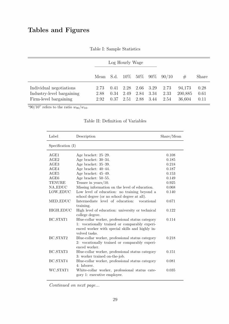
Figure 1 depicts labor supply and labor demand for three labor types, differentiated by
their productivity θi.
Figure 1 about here
2.3 Covered workers
Wages in the covered sector are characterized by the solution of a right-to-manage prob-
lem, which is the Nash solution of a bargaining problem in which the fallback position for
workers is to find employment in firms paying spot market wages wsi, while for firms the
fallback is to hire workers at monopoly union wages wmi. Then the union wage bargain
solves
wui = arg maxw∈[wsi,wmi]
(w − wsi)β (wmi − w)1−β
which implies the solution
wui = (1 − β)wsi + βwmi (3)
4

where β ∈ [0, 1] parametrizes the union’s bargaining power. One extreme case of such a
right-to-manage model is the monopoly union model (β = 1), in which unions have the
power to set wages unilaterally. In the other extreme (β = 0), wages of covered workers
are identical to wages of uncovered workers at the spot wage. Depending on unions’
bargaining power, the wage agreed on by firms and unions, wui, is located somewhere
between these extremes.
To determine the wage under right-to-manage we have yet to find the monopoly union
wage. The monopoly union chooses the wage wmi so as to maximize expected utility of
LSu (wmi) covered workers (affiliated with covered firms),
LD (wmi |θi, c)
LSu (wmi)
u(wmi) +LS
u (wmi) − LD (wmi |θi, c)
LSu (wmi)
u (w) ,
where the union takes productivity θi and the capital stock Kui = c as given. Utility u (·)is concave, though not necessarily strictly concave function of the wage. Without loss of
generality u (·) can be normalized such that u (w) = 0.5 So the monopoly union wage
maximizes
LD (wmi |θi, c)
LSu (wmi)
u(wmi).
It is standard that the interior solution to the maximization problem of the monopoly
union can be characterized by the tangency condition of labor demand and union indif-
ference curves, as depicted in Figure 1 (McDonald and Solow 1981, Oswald 1982, Farber
1986). Given the constant elasticity of the labor demand curve, the first-order condition
of the union maximization problem yields
u′ (wmi)wmi
u (wmi)=
1
α+ ε (4)
as long as the solution satisfies wmi ≥ wsi.
Since u′w/u is decreasing in w if u′w/u > 1 and because 1/α > 1 and ε ≥ 0, the
solution to condition (4) is unique. Note furthermore that it is independent of the pro-
ductivity parameter θi. Thus, the monopoly union wage is the same for all labor types i
as long as the solution of (4) is not smaller than wsi (see the thick solid upper curve in
5Maximization of a Benthamite utility function
LD (wmi |θi, c )u(wmi)
yields almost identical results. In fact, the first-order condition then becomes identical to condition (4)with ε (wmi) set to zero.
5

Figure 1 and notice that it is horizontal for small θ). By contrast, if the solution of (4) is
below wsi, for these labor types i markets clear. Then wsi = wmi and hence both wages
increase with total factor productivity according to (2).
Denote the specific total factor productivity for which labor markets just clear by
θ∗ such that wsi < wmi for all i with θ < θ∗ and wsi = wmi for all i with θ ≥ θ∗.
Although none of our results depend on this, it is convenient to assume that the latter
labor types actually exists; i.e., that for some labor types productivity is sufficiently high
such that both union wage mark-ups and unemployment vanish. Having obtained both
spot market and monopoly union wages, wages under right-to-manage (wui) are easily
determined from (3). Due to (2) the right-to-manage wui actually increases smoothly in
θ (assuming β < 1), even though monopoly union wages are constant for all θ < θ∗.
Finally, notice that the model admits the co-existence of covered and uncovered firms
in equilibrium, notwithstanding the fact that expected utility of covered and uncovered
workers may differ. To see this denote expected utility of a type-i worker initially affiliated
with a covered firm as vui and as vsi if initially affiliated with a uncovered firm. It is
intuitive to conclude that vui > vsi whenever wui > wsi. Under such conditions, positive
wage differences persist for the same reason that different types of human capital co-exist
even though they are remunerated at different rates: if switching costs from uncovered to
covered firms are sufficiently high, workers will refrain from incurring them.6
2.4 Stochastic dominance
A distribution described by the cumulative distribution function Y (x) is said to first-order
stochastically dominate another distribution Z (x) if Y (x) ≥ Z (x) , with strict inequality
holding for at least one x (Davidson 2008). We now argue that the wage distribution
induced under right-to-manage will first-order stochastically dominate that paid on spot
markets. In fact, the fraction of workers on spot markets earning more than any given
w ≥ wmin is strictly smaller than the respective fraction of workers employed in covered
firms. Comparing wages paid on labor markets with different productivity θ, from now
on we drop the subscripts i.
To generate intuition for this argument, it is useful to distinguish between two effects
which both work in the same direction. First, consider the direct union effect of raising
wages, abstracting from adverse effects on employment. If this wage increase is positive
everywhere, the union wage distribution would be located to the right of the spot wage at
6If for some labor type i these costs (in utility terms) exceeded vui − vsi > 0, the wage differencewui − wsi > 0 could persist. In a dynamic setting a complementary explanation could also be based onone-time costs such as re-training or moving costs. Obviously, such one-time costs incurred at the initialperiod need to be the larger, the greater vui − vsi and the smaller the rate of time preference.
6

each value of the cumulative distribution function (CDF). If the union wage is identical
to the spot market above some critical wage w∗, the union wage distribution function is
located below the spot wage distribution for all w ∈(wmin, w∗
)and coincides with the
spot wage distribution for all w ≥ w∗. This direct wage effect is shown in Figure 2 as the
first, rightward shift of the CDF of the spot wage distribution.
Figure 2 about here
Yet a second employment effect can be seen to add to the direct wage effect because—
comparing outcomes across labor markets with different θ—employment is positively cor-
related with wages. This implies that union wage setting crowds those (covered) workers
out of employment which earn relatively low wages. Thus, the employment effect skews
the wage distribution of covered workers towards higher wages. In the case of constant
labor supply (ε = 0), the employment effect would follow simply from the observation
that in all labor markets where wu > ws, it holds that Lu < Ls and
d log Lu
d log θ> 0 =
d log Ls
d log θ.
Similarly, if labor supply increases in the wage (ε > 0) and hence the right-hand side of
the above expression is positive, we can show that if wm > ws
d log Lu/d log θ
d log Ls/d log θ> 1,
simply because the elasticity of spot wages (with respect to total factor productivity θ) is
always higher than the respective elasticity of union wages under right-to-manage.7 Then,
ignoring the direct effect of unions on wages, the fraction of covered workers earning a
7In fact, total differentiation of (1) yields
d log wu
d log θ= 1 − α
d log Lu
d log θ
and a similar expression for the elasticity of spot market wages ws. From this it is easy to see that ifwm > ws,
d log Lu/d log θ
d log Ls/d log θ=
1 − d log wu/d log θ
1 − d log ws/d log θ> 1.
because differentiation of (3) yields
0 <d log wu
d log θ= (1 − β)
ws
wu
d log ws
d log θ<
d log ws
d log θ< 1.
7
wage greater than some given w > wmin is always less than the respective fraction of
uncovered workers. This implies that due to these negative employment effects, the union
wage distribution is below the spot wage distribution for all w ∈[wmin, wmax
)—even for
wages greater than w∗.
Because wage and employment effects work in the same direction, the union wage
distribution is everywhere below the spot wage distribution (over the whole support of
ws, see Figure 2). Stated differently, consider the fraction of covered workers who are paid
no more than some given w ≥ wmin. Then one observes that, first, this wage is paid in a
smaller number of labor markets (direct wage effect) and, second, in each labor market,
covered firms employ a smaller fraction of workers (employment effect). This result is
summarized by the following proposition:
Proposition 1 The union wage distribution first-order stochastically dominates the dis-
tribution of spot market wages. In fact, the fraction of covered workers who receive a wage
w ∈[wmin, wmax
)is strictly smaller than the respective fraction of uncovered workers.
First-order stochastic dominance has the following implications:
Corollary 2 At all quantiles τ ∈ [0, 1) monopoly union wages are strictly greater than
spot market wages.
Corollary 3 Mean wages of workers determined by a monopoly union are higher than
mean wages of workers on spot markets.
The union wage literature usually focuses on confirmation of Corollary 3 and tries to
quantify the actual gap in mean wages of the typical worker. Corollary 2, by contrast,
allows for a more direct and hence more powerful test for first-order stochastic dominance.
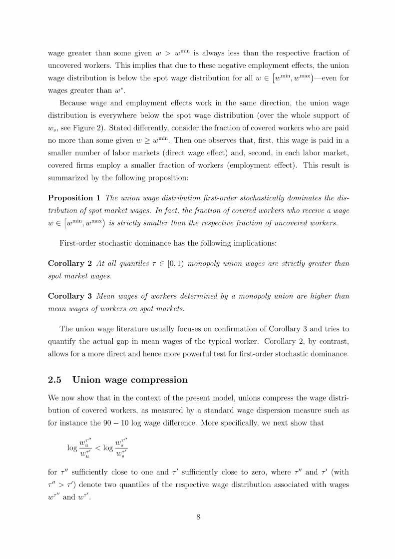
2.5 Union wage compression
We now show that in the context of the present model, unions compress the wage distri-
bution of covered workers, as measured by a standard wage dispersion measure such as
for instance the 90 − 10 log wage difference. More specifically, we next show that
logwτ ′′
u
wτ ′
u
< logwτ ′′
s
wτ ′
s
for τ ′′ sufficiently close to one and τ ′ sufficiently close to zero, where τ ′′ and τ ′ (with
τ ′′ > τ ′) denote two quantiles of the respective wage distribution associated with wages
wτ ′′
and wτ ′
.
8
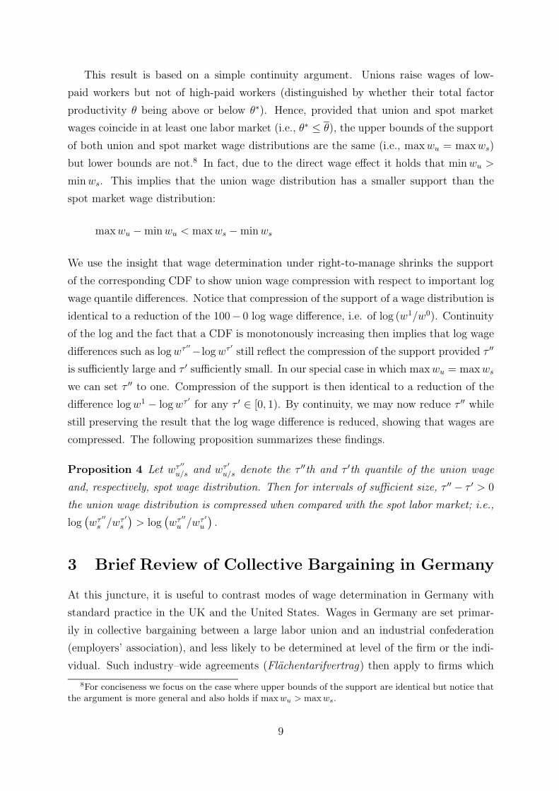
This result is based on a simple continuity argument. Unions raise wages of low-
paid workers but not of high-paid workers (distinguished by whether their total factor
productivity θ being above or below θ∗). Hence, provided that union and spot market
wages coincide in at least one labor market (i.e., θ∗ ≤ θ), the upper bounds of the support
of both union and spot market wage distributions are the same (i.e., max wu = maxws)
but lower bounds are not.8 In fact, due to the direct wage effect it holds that min wu >
min ws. This implies that the union wage distribution has a smaller support than the
spot market wage distribution:
max wu − min wu < max ws − min ws
We use the insight that wage determination under right-to-manage shrinks the support
of the corresponding CDF to show union wage compression with respect to important log
wage quantile differences. Notice that compression of the support of a wage distribution is
identical to a reduction of the 100− 0 log wage difference, i.e. of log (w1/w0). Continuity
of the log and the fact that a CDF is monotonously increasing then implies that log wage
differences such as log wτ ′′− log wτ ′
still reflect the compression of the support provided τ ′′
is sufficiently large and τ ′ sufficiently small. In our special case in which maxwu = maxws
we can set τ ′′ to one. Compression of the support is then identical to a reduction of the
difference log w1 − log wτ ′
for any τ ′ ∈ [0, 1). By continuity, we may now reduce τ ′′ while
still preserving the result that the log wage difference is reduced, showing that wages are
compressed. The following proposition summarizes these findings.
Proposition 4 Let wτ ′′
u/s and wτ ′
u/s denote the τ ′′th and τ ′th quantile of the union wage
and, respectively, spot wage distribution. Then for intervals of sufficient size, τ ′′ − τ ′ > 0
the union wage distribution is compressed when compared with the spot labor market; i.e.,
log(wτ ′′
s /wτ ′
s
)> log
(wτ ′′
u /wτ ′
u
).
3 Brief Review of Collective Bargaining in Germany
At this juncture, it is useful to contrast modes of wage determination in Germany with
standard practice in the UK and the United States. Wages in Germany are set primar-
ily in collective bargaining between a large labor union and an industrial confederation
(employers’ association), and less likely to be determined at level of the firm or the indi-
vidual. Such industry–wide agreements (Flachentarifvertrag) then apply to firms which
8For conciseness we focus on the case where upper bounds of the support are identical but notice thatthe argument is more general and also holds if max wu > maxws.
9

are members of the employers’ association who signed the contract in a specific region. In
our sample, 52% of the employees are covered by such agreements (last column of Table
I). If a firm is not member in an employers’ association, the firm can directly negotiate
pay and conditions with the union, resulting in a firm–level bargaining agreement (Fir-
mentarifvertrag or Haustarifvertrag).9 About 10% of the employees in our sample are
paid according to firm–level agreements. Thus, while firm–level bargaining is the usual
form of a collective bargaining agreement in the UK and the Unites States, in Germany
the firm is not the level at which bargaining commonly takes place. Empirical evidence as
well as theoretical considerations suggests that industry–wide and firm–level bargaining –
while following similar patterns – exhibit differences that are pronounced enough to war-
rant separate evaluation.10 The third category of wage agreements finally are described
by bilateral or individual negotiations between an employer and an employee, including
the mutually-agreed upon application of existing union contracts from other contexts or
circumstances (“Anwendungstarifvertrag”).
4 The GSES Dataset
Our empirical investigation is based on the 2001 cross-sectional sample of the German
Structure of Earnings Survey (GSES, or Gehalt- und Lohnstrukturerhebung). The GSES
is a linked employer-employee data set containing about 850,000 employees in roughly
22,000 firms from the private sector. It is conducted by the Federal Statistical Office
with the express purpose of assaying the structure of earnings in the German private
sector. The GSES is a stratified sample of firms with at least ten employees in a large
number of industries. Each firm is asked to report basic information regarding the firm
and in some more detail certain characteristics such as earnings, age, education, hours
worked, tenure and the like of each employee (for firms employing more then 20 workers
characteristics of a subsample of employees is reported). Besides being a large sample,
this relatively new dataset has a number of distinctive and attractive features. First, it
contains detailed and explicit information on union coverage, which is rarely observed in
continental Europe. Second, wages are uncensored firm information and are thus more
reliable than interview-based surveys (Jacobebbinghaus 2002). Third, hours worked are
9Instead of a union, the firm’s works council might settle an agreement. We pool those two cases inour analysis and refer to them both as “firm–level bargaining” or “firm–level agreements”.
10See Gurtzgen (2005, 2006) for empirical evidence as well as a discussion of possible causes for differentoutcomes of firm–level and industry–wide bargaining. Furthermore, Fitzenberger, Kohn, and Lembcke(2008), Kohn and Lembcke (2007), and Gerlach and Stephan (2006) estimate wage effects of coverage ofan individual worker by a collective contract. For Spain, Card and de la Rica (2006) provide evidence ondifferent wage outcomes when bargaining takes place at the firm–level or at the industry–wide.
10

directly observed. On the other hand, the GSES is not representative for all workers in
Germany because it basically omits the public sector and small firms with less than 10
employees; in addition, only cross-sectional information is available.11
The focus in this study is on male employees in West Germany aged 25-55 years, who
are working full time. We select this group of employees to minimize selection effects of
education and early retirement schemes. Given the regional heterogeneity found by Kohn
and Lembcke (2007), we focus on West Germany rather than Germany as a whole. After
reducing the sample along these lines as well as some minor criteria mentioned in the
Appendix, the sample contains approximately 330,000 white and blue collar employees.
As the most relevant variable for the present study, the GSES contains detailed infor-
mation on union coverage. Coverage is defined as employment under a contract which has
been determined in collective bargaining. The GSES report coverage separately for each
worker and not just as a dummy variable for a firm.12 It therefore occurs that within some
firms a number of individuals are reported to be covered (by industry–wide or firm–level
agreements), while others are not. In the subsequent analysis we focus on firm coverage in-
stead of individual coverage because firm–level coverage is closest to our theoretical model
and the estimates are better comparable to studies on Anglo-Saxon countries. There, at
least in the private sector, basically all workers are covered or no worker is covered. A
firm is considered covered if at least one worker is covered.13 We recode coverage status
of all individuals who are reported to be uncovered but work in a covered firm. After
modification therefore within each firm either all workers are uncovered, covered by an
industry–wide contract, or covered by a firm–level contract.
5 Econometric investigation
5.1 Econometric methodology
5.1.1 Conditional mean regression
The usual way to estimate trade union wage effects is to model the conditional mean of
log hourly wages of employees as a linear function of union coverage and a set of other
individual characteristics. As we distinguish for two types of union coverage (industry–
11A scientific–use–file (SUF) for the GSES has recently become available. Due to the higher level ofaggregation of industries in the SUF, we choose the on-site version of the data at the research data centerof the Hessian Statistical Office for our analysis.
12This is in contrast to the IAB establishment survey, which only provides a dummy variable on coveragefor each firm. The IAB establishment survey is used by Gurtzgen (2005, 2006) and Schnabel (2005).
13Since in most firms either a large share of employees is covered or no worker is covered, this choiceof threshold for firm coverage is not crucial.
11

wide and firm–level contracts, see the detailed description of the data above) a typical
specification for the log hourly wage, log w, would be
E [log w |X ] = Z ′βz + βiDi + βfDf . (5)
The base group being employees bargaining over their wages with firms at an individ-
ual bases, Di and Df indicate whether the firm of the respective worker is covered by a
industry–level or a firm–level collective agreement. Z is a collection of other characters of
the worker such as age, education, tenure, etc. (including also a constant). For brevity, de-
fine X ={Z, Di, Df
}. OLS estimates of βi and βf then report the effect of industry–wide
and firm–level bargaining on average log wages where, because the dependent variable is
measure in logs and the coefficient are relatively close to zero, the coefficients are usually
interpreted as a change of average wages in percentage points.
5.1.2 Conditional quantile regression
Least squares regressions focus on the wage level (average wage) only. Yet, in light of the
theoretical model above, union wage effects are likely to differ across the distribution. To
find evidence for the effect of unionization on the entire wage distribution, the empirical
investigation will focus on using a set of quantile regression estimates. One the one hand
this allows to describe and test union wage compression. On the other hand, it allows to
directly test for first-order stochastic dominance.
Specify the τth quantile function of log hourly wages conditional on the set of covariates
X as
qlog w(τ |X) = Z ′βz(τ) + βi (τ) Di + βf (τ) Df (6)
Quantile regression as introduced by Koenker and Bassett (1978) allows to estimate the
coefficients β (τ) =[βz (τ) , βi (τ) , βf (τ)
]by quantile τ considered. In our data, firms
with more than 20 employees do not report information on all of their employees, but only
on a sample of workers. While the computation of consistent regression quantiles is easy
to achieve, obtaining consistent standard errors is slightly more complicated. In addition,
usually reported standard errors may also be inconsistent in case of firm-specific wage
effects (clustering). Standard errors of the quantile regression coefficients then should
be adjusted appropriately. As at present standard software does not incorporate these
adjustments, we show in the appendix how to consistently estimate the covariance matrix
12

V AR(β(τ)), while accounting for both sampling weights and cluster effects.14
5.1.3 Decomposition of unconditional quantile functions
For the rest of this subsection ignore the difference between industry–wide and firm–level
collective bargaining. It is straightforward to decompose the difference of the uncondi-
tional sample quantile functions between covered and uncovered employees (denoted by
qcov(τ) and quncov(τ)) as follows:
qcov(τ) − quncov(τ) = [qcov(τ) − quc(τ)] + [quc(τ) − quncov(τ)] (7)
where quc(τ) is the estimated counterfactual quantile function, i.e. the quantile function
that would be generated for covered workers were they to be in work as uncovered em-
ployees. The first term on the right hand side gives the quantile treatment effect on the
treated (QTET), where treatment refers to union coverage. The second term captures
the effect of the workers’ characteristics. In terms of our theoretical model this means
that we evaluate the difference between covered and uncovered sector net of the differ-
ence induced by varying skills in the two sectors.15 This method is an extension of the
decomposition of average effects introduced by Blinder (1973) and Oaxaca (1973). For
quantile treatment effects the method usually employed is derived by Machado and Mata
(2005). In our analysis, we use the alternative approach proposed by Melly (2006) for
greater ease in computation.
Given the quantile function (6), the QTET is given by the coefficient βcov (τ). However,
if the coefficients βz(τ) are different for covered and uncovered workers (except for the
coefficient of the constant), computations of counterfactual quantile functions and hence
quantile treatment effects have to take account of this heterogeneity.16 We estimate
unconditional quantile functions for covered (separately for coverage at the industry and
at the firm–level) and uncovered employees using their sample counterparts17, which leaves
the counterfactual distribution to be estimated. Following Melly (2006), we estimate the
14In principle, bootstrapping is always an alternative approach for estimating V AR(β(τ)). But due tocomputational constraints, as in our case, it may not always be feasible.
15We assumed in Section 2 that the skill structure in the covered and uncovered sector is the same.16Variation of the coefficient on the constant is already captured by βcov (τ).17While Melly (2006) argues that estimating the unconditional quantile functions is more precise than
taking the sample quantiles, robustness checks using the scientific use file exhibited only marginal differ-ences. Since computational resources at the research data center are constrained and our sample size isvery large, we choose to use sample quantiles.
13
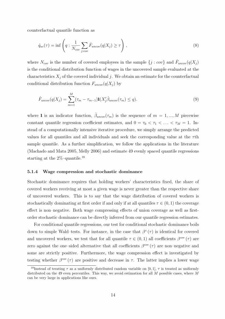
counterfactual quantile function as
quc(τ) = inf
(q :
1
Ncov
∑
j:cov
Funcov(q|Xj) ≥ τ
), (8)
where Ncov is the number of covered employees in the sample {j : cov} and Funcov(q|Xj)
is the conditional distribution function of wages in the uncovered sample evaluated at the
characteristics Xj of the covered individual j. We obtain an estimate for the counterfactual
conditional distribution function Funcov(q|Xj) by
Funcov(q|Xj) =
M∑
m=1
(τm − τm−1)11(X ′
jβuncov(τm) ≤ q). (9)
where 11 is an indicator function, βuncov(τm) is the sequence of m = 1, ..., M piecewise
constant quantile regression coefficient estimates, and 0 = τ0 < τ1 < . . . < τM = 1. In-
stead of a computationally intensive iterative procedure, we simply arrange the predicted
values for all quantiles and all individuals and seek the corresponding value at the τth
sample quantile. As a further simplification, we follow the applications in the literature
(Machado and Mata 2005, Melly 2006) and estimate 49 evenly spaced quantile regressions
starting at the 2%–quantile.18
5.1.4 Wage compression and stochastic dominance
Stochastic dominance requires that holding workers’ characteristics fixed, the share of
covered workers receiving at most a given wage is never greater than the respective share
of uncovered workers. This is to say that the wage distribution of covered workers is
stochastically dominating at first order if and only if at all quantiles τ ∈ (0, 1) the coverage
effect is non–negative. Both wage compressing effects of union coverage as well as first-
order stochastic dominance can be directly inferred from our quantile regression estimates.
For conditional quantile regressions, our test for conditional stochastic dominance boils
down to simple Wald–tests. For instance, in the case that βz (τ) is identical for covered
and uncovered workers, we test that for all quantile τ ∈ (0, 1) all coefficients βcov (τ) are
zero against the one–sided alternative that all coefficients βcov (τ) are non–negative and
some are strictly positive. Furthermore, the wage compression effect is investigated by
testing whether βcov (τ) are positive and decrease in τ . The latter implies a lower wage
18Instead of treating τ as a uniformly distributed random variable on [0, 1], τ is treated as uniformlydistributed on the 49 even percentiles. This way, we avoid estimation for all M possible cases, where Mcan be very large in applications like ours.
14

dispersion for covered workers compared to uncovered workers.19 Such simple Wald–tests
for stochastic dominance and wage compression become impractical when there is a lot of
heterogeneity in the union wage effects depending upon worker and firm characteristics.
Analogous to the conditional quantile regression coefficients, the quantile treatment
effects on the treated (QTET) are informative for our purposes and can be used for an
unconditional investigation of stochastic dominance. The QTET contrasts the wage dis-
tribution in the covered sector with the estimate of what this wage distribution would
have been in the hypothetical absence of coverage, holding workers’ characteristics con-
stant. The QTET can be analyzed easily even in the presence of heterogeneity where
the union wage effects depend upon worker and firm characteristics. Analogous to the
argument in footnote 19, the QTET at two given quantiles (τ ′′ and τ ′ < τ ′′) suggest union
wage compression whenever the QTET at τ ′′ is below the QTET at τ ′.
5.2 Descriptive Statistics
The dependent variable is a wage measure constructed as the logarithm of the actual
hourly wage in October 2001 (the reference period for the GSES). This was constructed
as the ratio of actual gross monthly wage or salary (excluding employer contributions to
social insurances) to reported hours (including overtime) in October 2001.
Some summary statistics describing the wage distribution, the number of observations,
and the coverage shares are provided in Table I. Further descriptive statistics on our
covariates are reported in column 3 of Table II. Among the 330,000 employees about 61%
are covered by an industry–wide or a firm–level bargaining agreement (upper panel of
Table I). The share decreases by 8 percentage points when we consider coverage at the
individual level, not at the firm–level (lower segment of Table I), indicating that there is
a non-negligible share of employees who themselves work in covered firms and who are
reported to be uncovered.20
Columns 2-5 of Table I report descriptive statistics on marginal wage distributions.
19For a worker with given characteristics Zi, union wages are compressed if at two quantiles τ ′ andτ ′′ > τ ′ it holds that
qcov (τ ′′|Zi) − qcov (τ ′|Zi) ≡ βcov(τ ′′) − βcov(τ ′) + Z ′i [βz (τ ′′) − βz (τ ′)]
< quncov (τ ′′|Zi) − quncov (τ ′|Zi) ≡ Z ′i [βz(τ ′′) − βz(τ ′)]) .
Simple rearranging of this inequality proves the claim. This implies in particular that union wages areeverywhere compressed, i.e. at all τ ′ and τ ′′, if the QTET as a function of τ decreases monotonically.
20Furthermore, the shares in the upper panel do not add up to 100% because about 3,500 employeeswork in firms that pay some of their employees according to a firm–level contract and, at the same time,some of their employees according to a industry–level contract. Such a situation is typically ruled out byGerman legislation but may occur in practice due to individual agreements or by extension of contractsagreed upon in the past which are still binding for parts of the workforce.
15
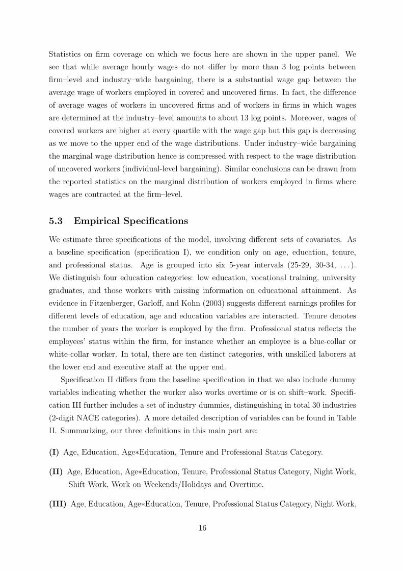
Statistics on firm coverage on which we focus here are shown in the upper panel. We
see that while average hourly wages do not differ by more than 3 log points between
firm–level and industry–wide bargaining, there is a substantial wage gap between the
average wage of workers employed in covered and uncovered firms. In fact, the difference
of average wages of workers in uncovered firms and of workers in firms in which wages
are determined at the industry–level amounts to about 13 log points. Moreover, wages of
covered workers are higher at every quartile with the wage gap but this gap is decreasing
as we move to the upper end of the wage distributions. Under industry–wide bargaining
the marginal wage distribution hence is compressed with respect to the wage distribution
of uncovered workers (individual-level bargaining). Similar conclusions can be drawn from
the reported statistics on the marginal distribution of workers employed in firms where
wages are contracted at the firm–level.
5.3 Empirical Specifications
We estimate three specifications of the model, involving different sets of covariates. As
a baseline specification (specification I), we condition only on age, education, tenure,
and professional status. Age is grouped into six 5-year intervals (25-29, 30-34, . . . ).
We distinguish four education categories: low education, vocational training, university
graduates, and those workers with missing information on educational attainment. As
evidence in Fitzenberger, Garloff, and Kohn (2003) suggests different earnings profiles for
different levels of education, age and education variables are interacted. Tenure denotes
the number of years the worker is employed by the firm. Professional status reflects the
employees’ status within the firm, for instance whether an employee is a blue-collar or
white-collar worker. In total, there are ten distinct categories, with unskilled laborers at
the lower end and executive staff at the upper end.
Specification II differs from the baseline specification in that we also include dummy
variables indicating whether the worker also works overtime or is on shift–work. Specifi-
cation III further includes a set of industry dummies, distinguishing in total 30 industries
(2-digit NACE categories). A more detailed description of variables can be found in Table
II. Summarizing, our three definitions in this main part are:
(I) Age, Education, Age∗Education, Tenure and Professional Status Category.
(II) Age, Education, Age∗Education, Tenure, Professional Status Category, Night Work,
Shift Work, Work on Weekends/Holidays and Overtime.
(III) Age, Education, Age∗Education, Tenure, Professional Status Category, Night Work,
16

Shift Work, Work on Weekends/Holidays, Overtime and Industry.
5.4 Results
5.4.1 OLS estimates
Table III reports OLS estimates of equation (5) for each of the above three specifications.
The estimate of βi can be found in the line saying “industry–wide bargaining”, the esti-
mate of βf in the line on “firm–level bargaining”. We find that in all three specifications
the union wage markup, as measured by βi and βf , is positive and significantly different
from zero. In our baseline specification the estimated union wage markup amounts to 9
log points for industry–wide bargaining and to 10 log points for firm–level bargaining. As
more covariates are added estimated markups decrease somewhat to 5.5 and 7 log points
for industry–wide and firm–level bargaining, but still remain statistically significant.
5.4.2 QR estimates
As argued in Section 5.1.4, union wages are compressed over the whole support of the
wage distribution if the quantile regression coefficient for coverage is decreasing over the
distribution. Union wages stochastically dominate the wage distribution of uncovered
workers if the coefficient is everywhere non–negative and positive for some quantiles. If
coefficients on covariates other than the union status (βz (τ)) are identical for all employ-
ees, both union wage compression and stochastic dominance can thus be easily detected
when plotting the respective coefficients βi (τ) and βf (τ) against quantiles τ . Consider
for instance the wage distribution of workers covered by industry–wide bargaining agree-
ments. If βi (τ) is found to decrease monotonically in τ , the distribution of these covered
workers is compressed everywhere with respect to the log wage difference inequality mea-
sure. More specifically, industry–wide bargaining is associated with a compressed wage
distribution with respect to e.g. the 90-10 wage percentile ratio if βi (.9) < βi (.1). If βi (τ)
is found to be non–negative for all quantiles and positive for some quantiles, the wage
distribution of this type of covered workers stochastically dominates the wage distribution
of uncovered workers.
Figure 3 shows the estimates βi (τ) and βf (τ) for 19 different quantiles (τ = .05,.10,.15,. . .,.95).
Solid lines depict the union wage gap under industry–wide bargaining and dashed lines re-
fer to firm–level bargaining. Thin lines indicate 95 percent (pointwise) confidence bands.
In all three graphs we find both βi (τ) and βf (τ) everywhere positive, thus suggesting
stochastic dominance of covered wage distributions. Moreover, confidence bands are al-
most everywhere above zero. In fact, only in specification (III) for the highest quantile
17

can we not reject the hypothesis that the union wage markup is positive.
Considering the wage effects of industry–wide bargaining first (solid lines), we ob-
serve that in the baseline specification (I) βi (τ) is relatively flat for low quantiles, but
decreases sharply at the upper 20 percent of the wage distribution. With respect to the
90-10 wage percentile ratio the wage distribution of this type of covered workers is hence
compressed. Conditioning on other worker characteristics (specification II) and also on
industries (specification III), βi (τ) is monotonically decreases over the whole zero-one
interval. This indicates that under industry–wide bargaining wages are everywhere com-
pressed.
When bargaining takes place at the firm–level, stochastic dominance holds but wages
are not compressed. In fact, in our baseline specification (I) as well as in specification (II)
the wage distribution widens at the upper end of the wage distribution. In specification
(III), conditioning also on a detailed set of industries, βf (τ) remains almost flat. The
data therefore do not support the hypothesis that unions compress the wage distribution
if bargaining takes place at the firm–level and not on the industry–wide.
Comparing wages paid in firms covered by industry–wide and firm–level agreements,
Figure 3 shows strong differences of union wage effects at the upper end of the wage
distributions. While union wage markups are very similar for wages below the median
wage, markups decrease for higher wages if industry–wide agreements are applied and
increase for firm–level agreements.
Decomposition of unconditional quantile functions
Table IV reports the estimated quantile treatment effect on the treated (QTET). That
is, in contrast to the previously discussed results we now allow covered workers to have
different age-earnings profiles and also to differ with respect to the wage effects of other
characteristics (such as, e.g., industry). Estimating the QTET this way is a sensitivity
check of the previous results for conditional quantile effects and it shows explicitly the
coverage effects on the unconditional wage distribution of the covered. Note that due to
computational constraints at the research data center, we only estimate the QTET at the
four quintiles (20%,40%,60%,80%) and we can not provide standard errors.
The marginal wage distributions described in Table I reemerge in the column labeled
“total”, reporting differences of unconditional quantile functions. The decomposition we
present in the table tells us how strong is the effect that is attributable to actual union
coverage (“QTET”) and how strong is the effect that is due to differences in employees’
characteristics (“Char.”). Take for instance the first row in the upper panel of Table IV.
The table shows that, comparing wages of uncovered workers (base group) and workers
18

whose wages are bargained over at the firm–level, at the 20th percentile of the respective
wage distributions wages of covered workers are 0.197 log points greater than wages of
uncovered workers. Table IV now says that, considering specification (I) and holding
characteristics of covered workers constant, 0.088 (≡QTET) log points of this difference
are due to differences in the pay structure, i.e., due to different coefficients. That is,
had these covered workers been paid as are uncovered workers, their unconditional wage
would have been only 0.088 log points lower, not 0.197. The remaining difference of 0.110
log points is due to differences in the distribution of characteristics between covered and
uncovered employees.
There are two important insights to be gained from inspection of Table IV. First,
covered workers receive higher wages over the whole wage distribution. The QTET is
always positive implying stochastic dominance of the union wage distribution. That is,
if uncovered workers had the same distribution of covariates as the covered workers, the
marginal wage distribution of covered workers would still dominate the marginal wage
distribution of uncovered workers. This results holds true both when wages are determined
at the firm or at the industry–level.
The second finding is that the union wage effects lead to a compression of the wage
distribution. For both firm–level and industry–wide bargaining it holds quite generally
that the greater τ , the lower the QTET. The decline of the estimated QTET in the
quantile τ is comparable to the decline of the coefficients βi (τ) and βf (τ) depicted in
Figure 3. Thus, also in this more general formulation of model (6)—after all, coefficients
βz (τ) are not assumed to be identical for covered and uncovered workers—we find that
unions raise wages of covered workers and at the same time reduce the dispersion of wages,
confirming our theoretical results summarized in propositions 1 and 4.
6 Conclusion
This paper develops and tests implications of a right–to–manage model for the distribu-
tion of wages. The theoretical analysis implies that the union wage effect decreases when
moving up the wage distribution, implying that unions compress the union wage distribu-
tion. Moreover, the theoretical model predicts first-order stochastic dominance of union
wages. The implications of the theory are testable and were investigated empirically using
quantile regressions.
The analysis is based on the German Structure of Earnings Survey 2001, a large
linked employer–employee data set which allows to identify coverage by industry–wide
and firm–level collective agreement. We analyze both the effect of union coverage on the
19

conditional and the unconditional wage distribution. This is implemented by estimating
both the quantile regression coefficients for coverage dummies and the quantile treatment
effect for the treated (QTET), i.e. the covered employees. The empirical results show that
the union wage effects decline when moving up the wage distribution for industry–wide
bargaining but not for firm–level bargaining. First-order stochastic dominance is also
confirmed.
Future research should consider the endogeneity of the wage bargaining regime and
the selectivity of the uncovered workers in covered firms. Based on more recent data, it
will be possible to analyze whether the share of uncovered low wage workers in covered
firms has increased over time given that the coverage rates have declined over time and
there has been a trend towards higher wage dispersion in the lower part of the wage
distribution.
20

References
Angrist, J., V. Chernozhukov, and I. Fernandez-Val (2004): “Quantile Regres-
sion under Misspecification, with an Application to the U.S. Wage Structure,” Working
Paper 10428, NBER.
(2006): “Quantile Regression under Misspecification, with an Application to the
U.S. Wage Structure,” Econometrica, 74(2), 539–564.
Blau, F. D., and L. M. Kahn (1996): “International Differences in Male Wage In-
equality: Institutions versus Market Forces,” Journal of Political Economy, 104(4),
791–837.
Blinder, A. S. (1973): “Wage Discrimination: Reduced Form and Structural Esti-
mates,” Journal of Human Resources, 8(4), 436–455.
Brown, J. N., and O. Ashenfelter (1986): “Testing the Efficiency of Employment
Contracts,” Journal of Political Economy, 94(3), S40–S87.
Cahuc, P., and A. Zylberberg (2004): Labor Economics. MIT Press.
Card, D., and S. de la Rica (2006): “Firm-Level Contracting and the Structure of
Wages in Spain,” Industrial and Labor Relations Review, 59(4), 573–592.
Card, D., T. Lemieux, and W. C. Riddell (2003): “Unions and the Wage Struc-
ture,” in International Handbook of Trade Unions, ed. by J. T. Addison, and C. Schn-
abel, chap. 8, pp. 246–92. Edward Elgar, Cheltenham, UK.
Christofides, L. N. (1990): “Non-Nested Tests of Efficient Bargain and Labour De-
mand Models,” Economic Letters, 32, 91–96.
Christofides, L. N., and A. J. Oswald (1991): “Efficient and Inefficient Employment
Outcomes: A Study Based on Canadian Contract Data,” Research in Labor Economics,
pp. 173–90.
Davidson, R. (2008): “Stochastic Dominance,” in The New Palgrave Dictionary of
Economics, ed. by S. Durlauf, and L. Blume. Palgrave Macmillan, 2nd edn.
Farber, H. S. (1986): “The Analysis of Union Behavior,” in Handbook of Labor Eco-
nomics, ed. by O. Ashenfelter, and R. Layard, vol. 2, chap. 18, pp. 1039–1089. Elsevier
Science.
21

Fitzenberger, B., A. Garloff, and K. Kohn (2003): “Beschaftigung und Lohn-
strukturen nach Qualifikationen und Altersgruppen: Eine empirische Analyse auf Ba-
sis der IAB-Beschaftigtenstichprobe,” Mitteilungen aus der Arbeitsmarkt- und Berufs-
forschung, 36(4), 509–524.
Fitzenberger, B., and K. Kohn (2005): “Gleicher Lohn fur gleiche Arbeit? Zum
Zusammenhang zwischen Gewerkschaftsmitgliedschaft und Lohnstruktur in West-
deutschland 1985-1997,” Zeitschrift fur Arbeitsmarktforschung, 38(2/3).
Fitzenberger, B., K. Kohn, and A. C. Lembcke (2008): “Union Density and
Varieties of Coverage: The Anatomy of Union Wage Effects in Germany,” Discussion
Paper 08-012, ZEW Mannheim.
Froot, K. A. (1989): “Consistent Covariance Matrix Estimation with Cross-Sectional
Dependence and Heteroscedasticity in Financial Data,” Journal of Financial and Quan-
titative Analysis, 24(3), 333–355.
Gerlach, K., and G. Stephan (2006): “Pay Policies of Firms and Collective Wage
Contracts – An Uneasy Partnership?,” Industrial Relations, 45(1), 47–67.
Gurtzgen, N. (2005): “Rent-sharing: Does the bargaining regime make a difference?
Theory and empirical evidence,” Discussion Paper 05-15, ZEW Mannheim.
(2006): “Rent-Sharing and Collective Bargaining Coverage – Evidence from
Linked Employer-Employee Data,” Discussion Paper 05-90, ZEW Mannheim.
Hall, P., and S. J. Sheather (1988): “On the Distribution of a Studentized Quantile,”
Journal of the Royal Statistical Society, Series B, 50(3), 381–391.
Hendricks, W., and R. Koenker (1992): “Hierarchical Spline Models for Condi-
tional Quantiles and the Demand for Electricity,” Journal of the American Statistical
Association, 87(417), 58–68.
Jacobebbinghaus, P. (2002): “Die Lohnverteilung in Haushaltsdatensatzen und in
amtlich erhobenen Firmendaten,” Wirtschaft und Statistik, (3), 209–221.
Koenker, R. (1994): “Confidence Intervals for Regression Quantiles,” in Asymptotic
Statistics: Proceeding of the 5th Prague Symposium on Asymptotic Statistics, ed. by
P. Mandl, and M. Huskova. Physica, Heidelberg.
(2005): Quantile Regression. Cambridge University Press, Cambridge.
22

Koenker, R., and G. Bassett (1978): “Regression Quantiles,” Econometrica, 46(1),
33–50.
Kohn, K., and A. C. Lembcke (2007): “Wage Distributions by Bargaining Regime:
Linked Employer-Employee Data Evidence from Germany,” Discussion Paper 0813,
CEP.
Lewis, H. G. (1986): Union Relative Wage Effects. University of Chicago Press, Chicago.
Machado, J. A. F., and J. Mata (2005): “Counterfactual Decomposition of Changes
in Wage Distributions using Quantile Regression,” Journal of Applied Econometrics,
20(4), 445–465.
MaCurdy, T. E., and J. H. Pencavel (1986): “Testing Betwen Competing Models
of Wages and Employment Determination in Unionized Markets,” Journal of Political
Economy, 94(3), S3–S39.
McDonald, I. M., and R. M. Solow (1981): “Wage Bargaining and Employment,”
American Economic Review, 71, 896–908.
Melly, B. (2006): “Estimation of counterfactual distributions using quantile regression,”
Discussion paper, unpublished manuscript, University of St. Gallen.
Moulton, B. R. (1990): “An Illustration of a Pitfall in Estimating the Effects of Aggre-
gate Variables on Micro Units,” Review of Economics and Statistics, 72(2), 334–338.
Nickell, S. J., and M. Andrews (1983): “Unions, Real Wages and Employment in
Britain 1951-79,” Oxford Economic Papers, 35(Supplement), 183–206.
Oaxaca, R. (1973): “Male-female wage differentials in urban labour markets,” Interna-
tional Economic Review, 14, 693–709.
OECD (ed.) (2006): OECD Employment Outlook – Boosting Jobs and Incomes. Organ-
isation for Economic Co-operation and Development, Paris.
Oswald, A. (1982): “The Microeconomic Theory of the Trade Union,” Economic Jour-
nal, 92, 576–595.
Schnabel, C. (2005): “Gewerkschaften und Arbeitgeberverbande: Organisationsgrade,
Tarifbindung und Einflusse auf Lohne und Beschaftigung,” Zeitschrift fur Arbeitsmark-
tForschung, 38(2/3), 181–196.
23

Silverman, B. W. (1986): Density Estimation for Statistics and Data Analysis. Chap-
man and Hall, London.
Vogel, T. (2007): “Union wage compression in a Right-to-Manage model,” Discussion
Paper 2007-009, SFB 649.
Williams, R. L. (2000): “A Note on Robust Variance Estimation for Cluster-Correlated
Data,” Biometrics, 56, 645–646.
24

Standard Errors for Quantile Regression with Sam-
pling Weights and Clustering
When estimating M quantiles in a non-iid setting, the asymptotic distribution of β, where
β is a column vector with elements β(τ) is given by
√N(β − β) ∼ N(0, V AR) (10)
where V AR consists of M blocks given by:
V AR(τ, τ ′) = J(τ)−1Σ(τ, τ ′)J(τ ′)−1 (11)
with V AR(τ, τ ′) = V AR(β(τ), β(τ ′)). The elements of this sandwich formula are defined
as:
Σ(τ, τ ′) ≡ E[(τ − 11{Y < X ′β(τ)})(τ ′ − 11{Y < X ′β(τ ′)})XX ′] (12)
and
J(τ) ≡ E[fy(X′β(τ)|X)XX ′] = E[fu(0|X)XX ′], (13)
which holds even if the true model is non-linear and the linear specification is only an
approximation (Angrist, Chernozhukov, and Fernandez-Val 2006). fu denotes the density
of the error term; compare Hendricks and Koenker (1992), Koenker (2005), and Melly
(2006). We estimate V AR(τ, τ ′) by
V AR(β(τ), β(τ ′)) =1
NJ(τ)−1Σ(τ, τ ′)J(τ ′)−1 (14)
where bread and butter are estimated as
Σ(τ, τ ′) =1
N
N∑
i=1
(τ − 11{Yi < X ′
iβ(τ)})(τ ′ − 11{Yi < X ′
iβ(τ ′)})XiX′
i (15)
and
J(τ) =1
N
N∑
i=1
fiXiX′
i (16)
for the case without weights and without clustering. To estimate the density function we
use the “Powell Sandwich”
J(τ) =1
2NcN
N∑
i=1
11(|ui| < cN)XiX′
i (17)
25

and define cN as:
cN = min{sd(u), IQR(u)/1.34}{F−1(τ + hN ) − F−1(τ + hN )} (18)
Where the first term on the right hand side is a robust estimate of scale (Silverman 1986)
given by the minimum of the standard deviation of the residuals and the interquartile
range of the residuals (divided by 1.34). In the second part of the product F−1, empirical
quantile function (of the residuals), is evaluated at a range around the quantile of interest
given by the bandwidth hN . In analogy to Koenker (1994) the empirical quantile function
is derived as is an interpolated piecewise linear function of the ordered residuals. To
estimate the bandwidth hN we employ Hall and Sheater’s (1988) rule:
hN =1
N1/3z2/3
α [1.5s(τ)/s′′(τ)]1/3, (19)
where zα satisfies Φ(zα) = 1 − α/2 for the construction of 1 − α confidence intervals and
s(τ) denotes the sparsity function.21 As in Koenker (1994), we use the normal distribution
to estimate
s(τ)/s′′(τ) =f 2
2(f ′/f)2 + [(f ′/f)2 − f ′′/f ]=
φ(Φ(τ)−1)2
2(Φ(τ)−1)2 + 1. (20)
Analogously to Angrist, Chernozhukov, and Fernandez-Val (2004), we take account of
sampling weights by replacing (15) with
Σ(τ, τ ′) =1
N
N∑
i=1
w2i (τ − 11{Yi < X ′
iβ(τ)})(τ ′ − 11{Yi < X ′
iβ(τ ′)})XiX′
i (21)
and (16) with
J(τ) =1
N
N∑
i=1
wifiXiX′
i. (22)
Clustering allows for dependence of observations within clusters (see Froot (1989), Moul-
ton (1990), or Williams (2000) for the case of OLS). We take account of clustering at the
firm level and use sampling weights that indicate the inverse sampling probability of an
observation. We normalize by dividing the individual weight by the size of the represented
population,∑N
i=1 wi/Npop = 1. Acknowledging that the sampling weights in the GSES
21The sandwich formula is extensively described in Koenker (2005, pp. 79–80). Koenker also mentionsthe “Hendricks-Koenker sandwich”, which is employed by e. g., Fitzenberger, Kohn, and Lembcke (2008).
26

are equal for all individuals i = 1, ..., Nc within a cluster c, (21) and (22) generalize to
Σ(τ, τ ′) =1
N
C∑
c=1
w2c
Nc∑
i=1
Nc∑
j=1
Xic(τ −11{Yic < X ′
icβ(τ)})(τ ′−11{Yjc < Xjcβ(τ ′)})X ′
jc (23)
and
J(τ) =1
N
C∑
c=1
wc
Nc∑
i=1
ficXicX′
ic. (24)
German Structure of Earnings Survey 2001
The German Structure of Earnings Survey (GSES, Gehalts- und Lohnstrukturerhebung)
2001 is a linked employer-employee data set administered by the German Statistical Office
in accordance with European and German law (European Council Regulation (EC) No
530/1999, amended by EC 1916/2000; German Law on Wage Statistics, LohnStatG). It
is a sample of all firms in manufacturing and private service sectors with at least ten em-
ployees. Sampling takes place at the firm or establishment level. At a first stage, firms are
randomly drawn from every Federal State, where the sampling probability varies between
5.3% for the largest state (North Rhine-Westphalia) and 19.4% for the smallest (Bremen).
At the second stage, employees are randomly chosen from the firms sampled at the first
stage. The share of employees sampled depends upon the firm size and ranges between
6.25% for the largest firms and 100% for firms with less than 20 employees. The data set
provides sampling weights. The GSES 2001 is available for on-site use at Research Centers
of the Federal States’ Statistical Offices (FDZ) since 2005. This study uses an anonymized
use-file which includes all firms and employees from the original data except for one firm
in Berlin (the only firm in Berlin falling into NACE section C). Regional information is
condensed to 12 “states”, and some industries have been aggregated at the two-digit level.
Overall, the use-file consists of 22,040 sites with 846,156 sampled employees. We focus on
prime-age (25–55-year-old) male full-time employees in West Germany (without Berlin),
including both blue and white-collar workers. Employees in vocational training, interns,
and employees subject to partial retirement schemes are left out because compensation for
these groups does not follow the regular compensation schedule, but special regulations
or even special collective bargaining agreements apply. Individuals who worked less than
90% of their contractual working hours in October 2001 and individuals paid subject to
a collective contract with a missing identification number for the agreement are dropped.
Part-time and full-time employees are distinguished based on the employer’s assessment
27

recorded in the GSES. For blue-collar workers, actual working time and not contractual
working time is relevant for monthly payments. We exclude individuals with an actual
working time of more than 390 hours in October 2001. We analyze gross hourly wages
including premia. This measure is more appropriate than wages without premia if premia
are paid on a regular basis. We impose a lower bound of one euro for hourly wages.
28
Tables and Figures
Table I: Sample Statistics
Log Hourly Wage
Mean S.d. 10% 50% 90% 90/10 # Share
Individual negotiations 2.73 0.41 2.28 2.66 3.29 2.73 94,173 0.28Industry-level bargaining 2.88 0.34 2.49 2.84 3.34 2.33 200,885 0.61Firm-level bargaining 2.92 0.37 2.51 2.88 3.44 2.54 36,604 0.11
“90/10” refers to the ratio w90/w10.
Table II: Definition of Variables
Label Description Share/Mean
Specification (I)
AGE1 Age bracket: 25–29. 0.108AGE2 Age bracket: 30–34. 0.185AGE3 Age bracket: 35–39. 0.218AGE4 Age bracket: 40–44. 0.187AGE5 Age bracket: 45–49. 0.153AGE6 Age bracket: 50–55. 0.149TENURE Tenure in years/10. 0.925NA EDUC Missing information on the level of education. 0.068LOW EDUC Low level of education: no training beyond a
school degree (or no school degree at all).0.140
MED EDUC Intermediate level of education: vocationaltraining.
0.671
HIGH EDUC High level of education: university or technicalcollege degree.
0.122
BC STAT1 Blue-collar worker, professional status category1: vocationally trained or comparably experi-enced worker with special skills and highly in-volved tasks.
0.114
BC STAT2 Blue-collar worker, professional status category2: vocationally trained or comparably experi-enced worker.
0.218
BC STAT3 Blue-collar worker, professional status category3: worker trained on-the-job.
0.151
BC STAT4 Blue-collar worker, professional status category4: laborer.
0.081
WC STAT1 White-collar worker, professional status cate-gory 1: executive employee.
0.035
Continued on next page...
29

... table II continued
Label Description Share/Mean
WC STAT2 White-collar worker, professional status cate-gory 2: executive employee with limited procu-ration.
0.157
WC STAT3 White-collar worker, professional status cate-gory 3: employee with special skills or expe-rience who works on his own responsibility onhighly involved or complex tasks.
0.099
WC STAT4 White-collar worker, professional status cate-gory 4: vocationally trained or comparably ex-perienced employee who works autonomously oninvolved tasks.
0.100
WC STAT5 White-collar worker, professional status cate-gory 5: vocationally trained or comparably ex-perienced employee working autonomously.
0.039
WC STAT6 White-collar worker, professional status cate-gory 6: employee working on simple tasks.
0.007
Specification (II)
NIGHT Individual worked night shifts. 0.142SUNDAY Individual worked on Sundays or on holidays. 0.149SHIFT Individual worked shift. 0.221OVERTIME Individual worked overtime. 0.257
Specification (III)
SECTOR1 Mining and quarrying (NACE: 10–14) 0.018SECTOR2 Manufacture of food products, beverages and to-
bacco (NACE: 15–16)0.025
SECTOR3 Manufacture of textiles and textile products;leather and leather products (NACE: 17–19)
0.012
SECTOR4 Manufacture of wood and wood products; pulp,paper and paper products (NACE: 20–21)
0.037
SECTOR5 Publishing, printing and reproduction ofrecorded media (NACE: 22)
0.029
SECTOR6 Manufacture of coke, refined petroleum prod-ucts and nuclear fuel; chemicals and chemicalproducts (NACE: 23–24)
0.036
SECTOR7 Manufacture of rubber and plastic products(NACE: 25)
0.039
SECTOR8 Manufacture of other non-metallic mineral prod-ucts (NACE: 26)
0.031
SECTOR9 Manufacture of basic metals; fabricated metalproducts, except from machinery and equipment(NACE: 27–28)
0.071
SECTOR10 Manufacture of machinery and equipment n.e.c.(NACE: 29)
0.057
SECTOR11 Manufacture of electrical machinery and appa-ratus n.e.c. (NACE: 31)
0.028
SECTOR12 Manufacture of electrical and optical equipment;radio, television, and communication equipmentand apparatus (NACE: 30 + 32)
0.028
Continued on next page...
30

... table II continued
Label Description Share/Mean
SECTOR13 Manufacture of medical, precision and opticalinstruments, watches and clocks (NACE: 33)
0.022
SECTOR14 Manufacture of transport equipment (NACE:34–35)
0.067
SECTOR15 Manufacture n.e.c. (NACE: 36–37) 0.024SECTOR16 Electricity, gas and water supply (NACE: 40–
41)0.032
SECTOR17 Construction (NACE: 45) 0.066SECTOR18 Sale, maintenance and repair of motor vehicles
and motorcycles; retail sale of automotive fuel(NACE: 50)
0.026
SECTOR19 Wholesale trade and commission trade except ofmotor vehicles and motorcycles (NACE: 51)
0.052
SECTOR20 Retail trade, except from motor vehicles andmotorcycles; repair of personal and householdgoods (NACE: 52)
0.024
SECTOR21 Hotels and restaurants (NACE: 55) 0.010SECTOR22 Land transport; transport via pipelines; air
transport (NACE: 60 + 62)0.036
SECTOR23 Water transport (NACE: 61) 0.007SECTOR24 Supporting and auxiliary transport activities;
activities of travel agencies (NACE: 63)0.047
SECTOR25 Post and telecommunications (NACE: 64) 0.023SECTOR26 Financial intermediation, except from insurance
and pension funding; activities auxiliary to fi-nancial intermediation, except from insuranceand pension funding (NACE: 65 + 67.1)
0.018
SECTOR27 Insurance and pension funding, except compul-sory social security; activities auxiliary to insur-ance and pension funding (NACE: 66 + 67.2)
0.016
SECTOR28 Real estate activities; renting of machinery andequipment without operator and of personal andhousehold goods (NACE: 70–71)
0.011
SECTOR29 Computer and related activities (NACE: 72) 0.029SECTOR30 Research and development; other business ac-
tivities (NACE: 73–74)0.078
31

Table III: OLS Regression Results
Specification
(I) (II) (III)
Industry-level bargaining (βi) 0.089∗∗ (0.005) 0.070∗∗ (0.004) 0.055∗∗ (0.004)
Firm-level bargaining (βf) 0.103∗∗ (0.016) 0.080∗∗ (0.016) 0.070∗∗ (0.010)
Regressions account for sampling weights. Robust standard errors (accounting for samplingweights and clustering at the firm level) in parentheses. ∗∗ indicates significance at the 1% level.
Table IV: Decomposition of Unconditional Quantile Functions
Specification
(I) (II) (III)
Firm-level
bargaining total QTET Char. QTET Char. QTET Char.
τ = 0.2 0.197 0.088 0.110 0.069 0.128 0.073 0.124τ = 0.4 0.173 0.091 0.082 0.066 0.107 0.072 0.101τ = 0.6 0.162 0.093 0.069 0.063 0.098 0.072 0.090τ = 0.8 0.114 0.067 0.047 0.043 0.071 0.048 0.066
Industry-level
bargaining
τ = 0.2 0.189 0.108 0.081 0.090 0.099 0.083 0.106τ = 0.4 0.163 0.108 0.056 0.087 0.076 0.080 0.083τ = 0.6 0.138 0.103 0.035 0.080 0.057 0.070 0.068τ = 0.8 0.065 0.056 0.009 0.042 0.023 0.023 0.042
Decomposition of the sample quantile function difference of unionized (covered) and spot market(uncovered); qcov(τ) − quncov(τ).QTET: Quantile Treatment Effect on the Treated (qcov(τ)− quc(τ)). Char.: Impact of employees’(observed) characteristics (quc(τ) − quncov(τ)).
32
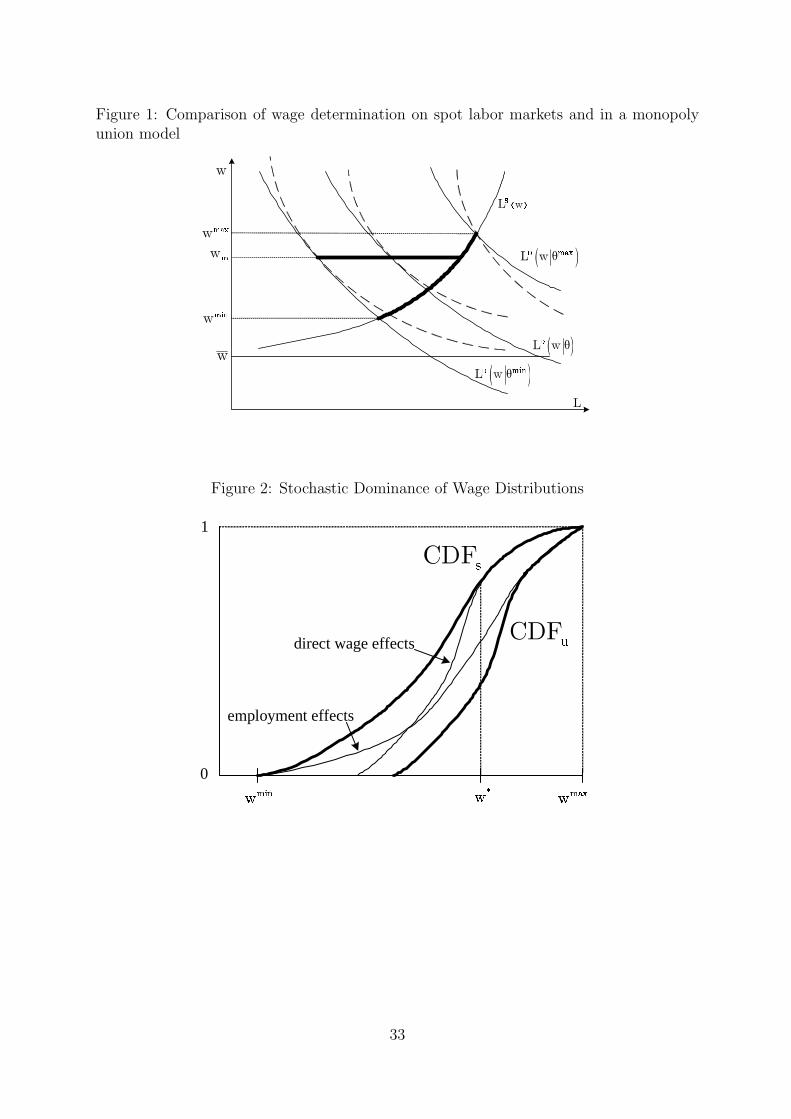
Figure 1: Comparison of wage determination on spot labor markets and in a monopolyunion model
L
w
���w
�w( )
� ���L w θ
( )� ���
L w θ
� ��wL
( )
L w θ
��w
w
Figure 2: Stochastic Dominance of Wage Distributions
��� �����employment effects
direct wage effects
0
1 �CDF �CDF
33

Figure 3: Quantile Regression Coefficients
Specification (I)
−.0
50
.05
.1.1
5.2
0 20 40 60 80 100Quantile
Specification (II)
−.0
50
.05
.1.1
5.2
0 20 40 60 80 100Quantile
Specification (III)
−.0
50
.05
.1.1
5.2
0 20 40 60 80 100Quantile
Solid lines refer to industry-level bargaining (βi), dashed lines to firm-levelbargaining (βf ). Base category: Individual wage negotiation. Thin lines depict95% confidence bands using standard errors that account for sampling weightsand clustering at the firm level. See Section 5.3 and Table II for a descriptionof specifications.
34

SFB 649 Discussion Paper Series 2008
For a complete list of Discussion Papers published by the SFB 649, please visit http://sfb649.wiwi.hu-berlin.de.
001 "Testing Monotonicity of Pricing Kernels" by Yuri Golubev, Wolfgang Härdle and Roman Timonfeev, January 2008.
002 "Adaptive pointwise estimation in time-inhomogeneous time-series models" by Pavel Cizek, Wolfgang Härdle and Vladimir Spokoiny, January 2008. 003 "The Bayesian Additive Classification Tree Applied to Credit Risk Modelling" by Junni L. Zhang and Wolfgang Härdle, January 2008. 004 "Independent Component Analysis Via Copula Techniques" by Ray-Bing Chen, Meihui Guo, Wolfgang Härdle and Shih-Feng Huang, January 2008. 005 "The Default Risk of Firms Examined with Smooth Support Vector Machines" by Wolfgang Härdle, Yuh-Jye Lee, Dorothea Schäfer and Yi-Ren Yeh, January 2008. 006 "Value-at-Risk and Expected Shortfall when there is long range dependence" by Wolfgang Härdle and Julius Mungo, Januray 2008. 007 "A Consistent Nonparametric Test for Causality in Quantile" by Kiho Jeong and Wolfgang Härdle, January 2008. 008 "Do Legal Standards Affect Ethical Concerns of Consumers?" by Dirk Engelmann and Dorothea Kübler, January 2008. 009 "Recursive Portfolio Selection with Decision Trees" by Anton Andriyashin, Wolfgang Härdle and Roman Timofeev, January 2008. 010 "Do Public Banks have a Competitive Advantage?" by Astrid Matthey, January 2008. 011 "Don’t aim too high: the potential costs of high aspirations" by Astrid Matthey and Nadja Dwenger, January 2008. 012 "Visualizing exploratory factor analysis models" by Sigbert Klinke and Cornelia Wagner, January 2008. 013 "House Prices and Replacement Cost: A Micro-Level Analysis" by Rainer Schulz and Axel Werwatz, January 2008. 014 "Support Vector Regression Based GARCH Model with Application to Forecasting Volatility of Financial Returns" by Shiyi Chen, Kiho Jeong and Wolfgang Härdle, January 2008. 015 "Structural Constant Conditional Correlation" by Enzo Weber, January 2008. 016 "Estimating Investment Equations in Imperfect Capital Markets" by Silke Hüttel, Oliver Mußhoff, Martin Odening and Nataliya Zinych, January 2008. 017 "Adaptive Forecasting of the EURIBOR Swap Term Structure" by Oliver Blaskowitz and Helmut Herwatz, January 2008. 018 "Solving, Estimating and Selecting Nonlinear Dynamic Models without the Curse of Dimensionality" by Viktor Winschel and Markus Krätzig, February 2008. 019 "The Accuracy of Long-term Real Estate Valuations" by Rainer Schulz, Markus Staiber, Martin Wersing and Axel Werwatz, February 2008. 020 "The Impact of International Outsourcing on Labour Market Dynamics in Germany" by Ronald Bachmann and Sebastian Braun, February 2008. 021 "Preferences for Collective versus Individualised Wage Setting" by Tito Boeri and Michael C. Burda, February 2008.
SFB 649, Spandauer Straße 1, D-10178 Berlin
http://sfb649.wiwi.hu-berlin.de
This research was supported by the Deutsche Forschungsgemeinschaft through the SFB 649 "Economic Risk".

022 "Lumpy Labor Adjustment as a Propagation Mechanism of Business Cycles" by Fang Yao, February 2008. 023 "Family Management, Family Ownership and Downsizing: Evidence from S&P 500 Firms" by Jörn Hendrich Block, February 2008. 024 "Skill Specific Unemployment with Imperfect Substitution of Skills" by Runli Xie, March 2008. 025 "Price Adjustment to News with Uncertain Precision" by Nikolaus Hautsch, Dieter Hess and Christoph Müller, March 2008. 026 "Information and Beliefs in a Repeated Normal-form Game" by Dietmar Fehr, Dorothea Kübler and David Danz, March 2008. 027 "The Stochastic Fluctuation of the Quantile Regression Curve" by Wolfgang Härdle and Song Song, March 2008. 028 "Are stewardship and valuation usefulness compatible or alternative objectives of financial accounting?" by Joachim Gassen, March 2008. 029 "Genetic Codes of Mergers, Post Merger Technology Evolution and Why Mergers Fail" by Alexander Cuntz, April 2008. 030 "Using R, LaTeX and Wiki for an Arabic e-learning platform" by Taleb Ahmad, Wolfgang Härdle, Sigbert Klinke and Shafeeqah Al Awadhi, April 2008. 031 "Beyond the business cycle – factors driving aggregate mortality rates" by Katja Hanewald, April 2008. 032 "Against All Odds? National Sentiment and Wagering on European Football" by Sebastian Braun and Michael Kvasnicka, April 2008. 033 "Are CEOs in Family Firms Paid Like Bureaucrats? Evidence from Bayesian and Frequentist Analyses" by Jörn Hendrich Block, April 2008. 034 "JBendge: An Object-Oriented System for Solving, Estimating and Selecting Nonlinear Dynamic Models" by Viktor Winschel and Markus Krätzig, April 2008. 035 "Stock Picking via Nonsymmetrically Pruned Binary Decision Trees" by Anton Andriyashin, May 2008. 036 "Expected Inflation, Expected Stock Returns, and Money Illusion: What can we learn from Survey Expectations?" by Maik Schmeling and Andreas Schrimpf, May 2008. 037 "The Impact of Individual Investment Behavior for Retirement Welfare: Evidence from the United States and Germany" by Thomas Post, Helmut Gründl, Joan T. Schmit and Anja Zimmer, May 2008. 038 "Dynamic Semiparametric Factor Models in Risk Neutral Density Estimation" by Enzo Giacomini, Wolfgang Härdle and Volker Krätschmer, May 2008. 039 "Can Education Save Europe From High Unemployment?" by Nicole Walter and Runli Xie, June 2008. 040 "Solow Residuals without Capital Stocks" by Michael C. Burda and Battista Severgnini, August 2008. 041 "Unionization, Stochastic Dominance, and Compression of the Wage Distribution: Evidence from Germany" by Michael C. Burda, Bernd Fitzenberger, Alexander Lembcke and Thorsten Vogel, March 2008
SFB 649, Spandauer Straße 1, D-10178 Berlin http://sfb649.wiwi.hu-berlin.de
This research was supported by the Deutsche
Forschungsgemeinschaft through the SFB 649 "Economic Risk".