Eindhoven University of Technology
MASTER
Hydrodynamics of fluidized beds under reaction conditions
Grim, R.
Award date:2015
Link to publication
DisclaimerThis document contains a student thesis (bachelor's or master's), as authored by a student at Eindhoven University of Technology. Studenttheses are made available in the TU/e repository upon obtaining the required degree. The grade received is not published on the documentas presented in the repository. The required complexity or quality of research of student theses may vary by program, and the requiredminimum study period may vary in duration.
General rightsCopyright and moral rights for the publications made accessible in the public portal are retained by the authors and/or other copyright ownersand it is a condition of accessing publications that users recognise and abide by the legal requirements associated with these rights.
• Users may download and print one copy of any publication from the public portal for the purpose of private study or research. • You may not further distribute the material or use it for any profit-making activity or commercial gain
Ruden Grim, 0719066
Graduation committee:
prof. dr. ir. Martin van Sint Annaland
dr. ir. Fausto Gallucci
dr. ir. John van der Schaaf
Ildefonso Campos Velarde, MSc
Hydrodynamics of fluidized beds under reaction conditions
Final report, June 2014
Ruden Grim


Summary
I
Summary
Gas-solid fluidized bed reactors have been used extensively in chemical industry since the 1960s. In recent
years, their advantages have been proposed to be used in innovative CO2 neutral processes to produce energy
carriers or chemicals. One of these innovative processes is known as the MILENA process, which uses a
fluidized bed reactor set-up to produce methane out of woody biomass. Just as many other fluidized bed
applications, the MILENA process is carried out at temperatures which could go up to 1000 °C. However,
due to experimental challenges, to date, only few is known about fluidized bed behavior at high temperatures.
In order to investigate both emulsion and bubble phase simultaneously, an experimental set-up has been
proposed recently, which allows to use particle image velocimetry (PIV) combined with digital image analysis
(DIA) at high temperature.
In this work, a start has been made to describe the hydrodynamics of fluidized beds at high temperatures. At
first, minimum fluidization velocity of differently sized glass particles, for different fluidization gases and at
different temperatures have been determined. The experiments revealed that minimum fluidization behavior
could only be explained for ordinary gases as nitrogen and air at room temperature by commonly used
correlations. At high temperatures less easy fluidization was observed.

II
Possibly, the differences in predicted and experimental behavior could be explained by a change in bed
porosity at high temperature. In order to cancel out the effect of particle and gas properties on the porosity at
high temperature, their influence on room temperature minimum fluidization porosity had been established
first. Finally, it was found that temperature adds an additional effect to the bed porosity.
It is expected that the found phenomena could be explained with changing van der Waals force. For smaller
particles, these forces will get dominant compared to the gravitational force. Due to cohesion, cluster
formation is enhanced, which will lead to higher bed porosity and less easy fluidization. The additional effect
of high temperature fluidization is expected to have influence on the Hamaker constant. This constant is a
function of temperature and since it determines the magnitude of the van der Waals force, temperature has a
major influence on the formation of particle aggregates.
Acknowledgement
III
Acknowledgement
More than a year ago, I informed Martin van Sint Annaland about the possibilities to do a graduation project
within the SMR group. One of the main criteria, for me, was that the project had to be challenging. After all,
indeed, this project really turned out to be challenging, since we were dealing with a newly developed
experimental technique, which leaded to new experimental results as well. Thank you Martin for giving me
the opportunity and confidence to work in this group and on this project in particular.
Besides, I am very grateful to Fausto Gallucci. He gave me the freedom to carry out all the experiments I
wanted to do. Without his approval, I would not have been able to cover all the work I intended to do. John
van der Schaaf, thank you for your willingness to be part of the graduation committee. I really appreciated
your critical attitude.
The last member of the graduation committee was at the same time my daily supervisor. Ildefonso Campos
Velarde guided my through this project and together we came up with ideas to get the desired results. I really
appreciated that it was always possible to drop by your office for a talk about the project or whatsoever. I
think we have been a pretty good team for the past months. Of course, we obtained quite some interesting
results, but on the other hand we had some bad luck too. Anyway, I have not encountered any disagreement
or signs of stress the past months, which made it pleasant to work with you!

IV
For the technical support I have to thank the technicians at SMR and in particular Joost Kors. Joost
supported me in many different ways, so I was able to carry out all my experiments. I really have to touch on
his neat way of working and his talent to come up with creative ideas.
Of course, I would like to say thanks to all people at SMR and students in the student room for the pleasant
working atmosphere, the morning coffee breaks, nice borrels and of course many more things. However, I
want to take out some people who really deserve a thumb up. Mariët, thanks for helping me with the DPM
simulations and the handling of the polymer particles. Kay, José, Arash, Alvaro, you were the beating heart of
the SMR football team. Thank you for letting me join the team. I really enjoyed the football lunch breaks.
Paul, thank you for being our loyal supporter. In good and bad times..
After all, the biggest ‘thank you’ should go to my friends and family. Without any doubt, I have the best
friends in the world. They really made me enjoy the time I stayed in Eindhoven. I am really grateful to my
parents. They have always supported me and they have given me the opportunity to take chances. Besides
confidence, they gave me the financial support I needed the past five years. It feels good to be able to finish
this period in my life with this report.
Ruden Grim
June 2014
Table of contents
V
Table of contents
Summary ................................................................................................................................................................................ I
Acknowledgement ........................................................................................................................................................... III
Table of contents ............................................................................................................................................................... V
List of figures ................................................................................................................................................................... VII
List of tables .......................................................................................................................................................................XI
Notation ......................................................................................................................................................................... XIII
1 Introduction ................................................................................................................................................................ 1
1.1 MILENA technology ....................................................................................................................................... 2
1.2 Fluidized beds ................................................................................................................................................... 4
1.3 Temperature effects on hydrodynamics ....................................................................................................... 5
1.4 Measurement techniques ................................................................................................................................. 6
1.5 Particle image velocimetry coupled with digital image analysis................................................................. 8
1.6 Endoscopic laser particle image velocimetry with digital image analysis................................................. 9
VI
1.7 State of the art ................................................................................................................................................. 10
2 Experimental study on high temperature fluidization ....................................................................................... 11
2.1 Introduction..................................................................................................................................................... 12
2.2 Experimental procedure ................................................................................................................................ 20
2.3 Results and discussion ................................................................................................................................... 22
2.4 Conclusions ..................................................................................................................................................... 26
3 Experimental study on the porosity at minimum fluidization .......................................................................... 29
3.1 Introduction..................................................................................................................................................... 30
3.2 Experimental procedure ................................................................................................................................ 32
3.3 Results and discussion ................................................................................................................................... 37
3.4 Conclusions ..................................................................................................................................................... 47
4 Hydrodynamics of bubbling fluidized beds......................................................................................................... 49
4.1 Introduction..................................................................................................................................................... 50
4.2 Experimental procedure ................................................................................................................................ 51
4.3 Results and discussion ................................................................................................................................... 53
4.4 Conclusions ..................................................................................................................................................... 57
5 Forces in fluidized beds .......................................................................................................................................... 59
5.1 Introduction..................................................................................................................................................... 60
5.2 Discrete particle model .................................................................................................................................. 64
5.3 Results and discussion ................................................................................................................................... 64
5.4 Conclusions ..................................................................................................................................................... 69
Conclusion and recommendations ................................................................................................................................. 71
References .......................................................................................................................................................................... 73
Appendix 1: Determination of minimum fluidization velocity ................................................................................. 85
Appendix 2: Overview of literature values for minimum fluidization porosity for Geldart B particles ............. 89
Appendix 3: Determination of porosity at minimum fluidization ............................................................................ 95

List of figures
VII
List of figures
Figure 1.1: Ecological footprints of different biofuels compared to fossil fuels .......................................................................... 3
Figure 1.2: Different routes for methane conversion ........................................................................................................................ 3
Figure 1.3: Schematic representation of MILENA process ............................................................................................................. 4
Figure 1.4: Measurement techniques in fluidized bed reactors ........................................................................................................ 7
Figure 2.1: Visualization of Ergun equation ...................................................................................................................................... 14
Figure 2.2: Constant C1 for a wide range of conditions .................................................................................................................. 14
Figure 2.3: Constant C2 for a wide range of conditions .................................................................................................................. 14
Figure 2.4: Experimental set-up to determine minimum fluidization velocity ............................................................................ 21
Figure 2.5: Schematic representation of the procedure to estimate the minimum fluidization velocity ................................ 21
Figure 2.6: Gas density as function of gas viscosity for air, nitrogen, helium and hydrogen. Markers placed at 25 °C, 50
°C, 100 °C, up to 500 °C ............................................................................................................................................................ 22
Figure 2.7: Minimum fluidization velocity as a function of temperature for 528 μm glass beads and fluidization with air,
nitrogen, helium and hydrogen .................................................................................................................................................. 24
Figure 2.8: Minimum fluidization velocity as a function of temperature for 263 μm glass beads and fluidization with air,
nitrogen, helium and hydrogen .................................................................................................................................................. 25
Figure 2.9: 1/Remf as a function of 1/Ar for 528 μm glass beads and fluidization with air, nitrogen, helium and hydrogen
......................................................................................................................................................................................................... 27

VIII
Figure 2.10: 1/Remf as a function of 1/Ar for 263 μm glass beads and fluidization with air, nitrogen, helium and
hydrogen ........................................................................................................................................................................................ 28
Figure 3.1: Porosity at minimum fluidization as a function of temperature as established by a) Subramani et al. and b)
Formisani et al. ............................................................................................................................................................................. 31
Figure 3.2: Experimental porosity at minimum fluidization as a function of predicted porosity at minimum fluidization
according to a) Subramani et al., b) Broadhurst and Becker and c) Fatah ......................................................................... 33
Figure 3.3: Representation of the procedure to estimate the porosity at minimum fluidization ............................................. 34
Figure 3.4: Schematic representation of cold-flow PIV/DIA set-up ........................................................................................... 35
Figure 3.5: Gas density as function of gas viscosity for helium and 0.19:0.81 neon:hydrogen mixture. Markers placed
every 50 °C .................................................................................................................................................................................... 36
Figure 3.6: Experimental values for the porosity at minimum fluidization as a function of Archimedes number for
different sized glass beads and fluidization with different gases and gas mixtures .......................................................... 37
Figure 3.7: Experimental porosity at minimum fluidization as a function of predicted porosity at minimum fluidization
for present experimental work for a) Subramani et al., b) Broadhurst and Becker and c) Fatah .................................. 40
Figure 3.8: Experimental values for the porosity at minimum fluidization as a function of particle size for fluidization
with glass beads and different gases and gas mixtures .......................................................................................................... 41
Figure 3.9: Pseudo 2D fluidized bed snapshot of a) 528 μm glass beads fluidization with N2 and b) 100 μm glass beads
fluidization with N2. Excess velocity (u0 – umf) in both cases equal to 0.05 m s-1. ........................................................... 41
Figure 3.10: Experimental porosity at minimum fluidization as a function of predicted porosity at minimum fluidization
for a) Equation 3.5 and b) Equation 3.6 .................................................................................................................................. 43
Figure 3.11: Porosity at minimum fluidization as function of Archimedes number for different degrees of sphericity..... 44
Figure 3.12: Reynolds number at minimum fluidization as a function of Archimedes number for gas mixtures having the
same gas properties at different temperature .......................................................................................................................... 45
Figure 3.13: Porosity at minimum fluidization plotted as a function of temperature for hydrogen and helium for a) 528
μm glass beads and b) 250 μm glass beads .............................................................................................................................. 46
Figure 3.14: Experimental porosity at minimum fluidization as a function of predicted porosity at minimum fluidization
for fluidization both at room temperature as well as at elevated temperatures ................................................................ 47
Figure 3.15: Experimental Reynolds number at minimum fluidization as a function of predicted Reynolds number at
fluidization with Carman-Kozeny and Equation 3.8. a) Full range, b) zoomed in on Reynolds number up to 2.0 and
c) zoomed in on Reynolds number up to 1.0 .......................................................................................................................... 48
Figure 4.1: Equivalent bubble diameter as a function of bed height for fluidization with nitrogen, excess flow rates of
0.10 m s-1, 0.32 m s-1 and 0.52 m s-1. a) 528 μm glass beads and b) 177 μm glass beads ................................................ 54
Figure 4.2: Average bed porosity and emulsion phase porosity as a function of excess flow rate for fluidization with
nitrogen and 177 μm and 528 μm glass beads ........................................................................................................................ 54
Figure 4.3: Total number of bubbles as a function of equivalent bubble diameter for fluidization with nitrogen and 177
μm and 528 μm glass beads (u0-umf = 0.32 m s-1). Amount of dubble frame images is equal to 1500. ........................ 54
Figure 4.4: Difficulties for bubble detection using DIA for fluidization with 177 μm glass beads ........................................ 55
IX
Figure 4.5: Bubble rise velocity as a function of equivalent bubble diameter for fluidization with nitrogen and a) 528 μm
glass beads and b) 177 μm glass beads. Constants by Mudde et al. and Hilligardt and Werther................................... 56
Figure 4.6: Visual bubble flow rate as function of dimensionless bed height for fluidization with nitrogen and a) 528 μm
glass beads and b) 177 μm glass beads. .................................................................................................................................... 56
Figure 4.7: Bubble rise velocity as a function of equivalent bubble diameter for fluidization with nitrogen and a) 528 μm
glass beads and b) 177 μm glass beads. Constants determined experimentally. ............................................................... 56
Figure 5.1: The effect of particle density on the loosely packed bed porosity (Equation 5.4) with AH = 6.5 x 10⁻²⁰ J for 1)
ρp = 10 000 kg m-3, 2) ρp = 2 500 kg m-3 and 3) ρp = 100 kg m-3 ........................................................................................ 62
Figure 5.2: The effect of Hamaker constant on the loosely packed bed porosity (Equation 5.4) with ρp = 2 500 kg m-3 for
1) AH = 6.5 x 10⁻²¹ J, 2) AH = 6.5 x 10⁻²⁰ J and 3) AH = 6.5 x 10⁻¹⁹ J ................................................................................. 62
Figure 5.3: Liquid bridge formation between two equally sized spheres ..................................................................................... 63
Figure 5.4: Porosity at minimum fluidization as a function of Archimedes number. A comparison between experimental
values and DPM simulations ...................................................................................................................................................... 66
Figure 5.5: Porosity at minimum fluidization as a function of particle diameter, including Yang et al. correlation to
predict porosity of loosely packed bed ..................................................................................................................................... 66
Figure 5.6: Force ratio Fvdw/Fg as a function of particle size for separation distances between 1.65 Å and 4.00 Å ............ 67
Figure 5.7: Force ratio Fvdw/Fe as a function of particle size for separation distance of 4.00 Å ............................................. 68
Figure 5.8: Force ratio FvdW/Fg as a function of particle diameter for different values of the refractive index. As
separation distance 1.65 Å has been used, 2 500 kg m-3 has been used as particle density. ........................................... 69

X

List of tables
XI
List of tables
Table 2.1: Available literature correlations to predict minimum fluidization velocity ............................................................... 16
Table 2.2: Specification of particles used for minimum fluidization determination at high temperature .............................. 21
Table 3.1: Porosity at minimum fluidization conditions ................................................................................................................. 30
Table 3.2: Available literature correlations to predict porosity at minimum fluidization .......................................................... 32
Table 3.3: Specification of particles used for the determination of the porosity at minimum fluidization ........................... 35
Table 3.4: Overview experimental results for bed porosity spherical particles ........................................................................... 38
Table 3.5: Fitting parameters correlations to predict the porosity at minimum fluidization .................................................... 42
Table 3.6: Fitting parameters correlations to predict the porosity at minimum fluidization at elevated temperatures ....... 46
Table 4.1: Specification of particles used for the determination of the fluidized bed hydrodynamics ................................... 52
Table 5.1: Settings for DPM simulations to investigate importance of interparticle forces ..................................................... 65

XII
Notation
XIII
Notation
Symbols
A, B, C, constants [-]
A area [m2]
A0 catchment area [m2]
AH Hamaker constant [J]
a, b, c, constants [-]
d diameter [m]
F force [N]
fp friction factor [-]
g gravitational constant [m s-2]
h height [m]
h Planck constant [J s]
k Boltzmann constant [J K-1]
M mass [kg]
N number [-]
XIV
n number [-]
n refractive index [-]
p pressure [Pa]
q charge [C]
r distance [m]
s separation distance [m]
s standard deviation [-]
T temperature [K]
t bed depth [m]
t student-t value [-]
u velocity [m s-1]
v frequency [s-1]
x mean [-]
x, y, z coordinates [-]
Greek
α confidence level [-]
γ surface tension [N m-1]
Δ difference [-]
ε dielectric constant [-]
ε porosity [-]
ε0 vacuum permittivity [F m-1]
μ expected value [-]
μ viscosity [Pa s]
ρ density [kg m-3]
φ sphericity [-]
ψ visual bubble flow rate [-]
Subscripts
0 initial
2D two dimensional
3D three dimensional
avg average
b bubble
e emulsion

Notation
XV
exp experimental
g gas
g gravitational
mf minimum fluidization
p particle
pred predicted
px pixel
s solid
t terminal
vdW van der Waals
Dimensionless groups
Re Reynolds number
Ar Archimedes number
Abbreviations
DIA digital image analysis
DPM discrete particle model
PIV particle image velocimetry
RPT radioactive particle tracking

XVI

Introduction
1
1 Introduction
Two worldwide problems we are facing nowadays both deal with fossil fuels. On the one hand, fossil fuel reserves are declining,
which makes our future energy needs uncertain. Besides, the combustion of fossil fuels produces CO2, which is one of the main
contributors to the global warming scenario. A possible solution to cope with both problems is the gasification of woody biomass
into bio-methane. A commercial technology to convert biomass into bio-methane was introduced a decade ago by the Energy
research Centre of the Netherlands (ECN). The so-called MILENA technology uses a fluidized bed reactor operated at high
temperatures as a gasifier. In order to improve the operation of fluidized beds, hydrodynamics at high temperatures have to be
clarified. Since no conformity is reached on this topic in literature, an endoscopic laser particle image velocimetry combined with
digital image analysis (PIV/DIA) set-up has been proposed to study the effects of elevated temperatures on the hydrodynamics of
fluidized beds.
2
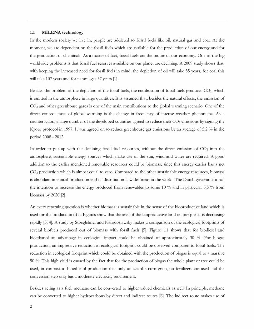
1.1 MILENA technology
In the modern society we live in, people are addicted to fossil fuels like oil, natural gas and coal. At the
moment, we are dependent on the fossil fuels which are available for the production of our energy and for
the production of chemicals. As a matter of fact, fossil fuels are the motor of our economy. One of the big
worldwide problems is that fossil fuel reserves available on our planet are declining. A 2009 study shows that,
with keeping the increased need for fossil fuels in mind, the depletion of oil will take 35 years, for coal this
will take 107 years and for natural gas 37 years [1].
Besides the problem of the depletion of the fossil fuels, the combustion of fossil fuels produces CO2, which
is emitted in the atmosphere in large quantities. It is assumed that, besides the natural effects, the emission of
CO2 and other greenhouse gases is one of the main contributions to the global warming scenario. One of the
direct consequences of global warming is the change in frequency of intense weather phenomena. As a
counteraction, a large number of the developed countries agreed to reduce their CO2 emissions by signing the
Kyoto protocol in 1997. It was agreed on to reduce greenhouse gas emissions by an average of 5.2 % in the
period 2008 - 2012.
In order to put up with the declining fossil fuel resources, without the direct emission of CO2 into the
atmosphere, sustainable energy sources which make use of the sun, wind and water are required. A good
addition to the earlier mentioned renewable resources could be biomass; since this energy carrier has a net
CO2 production which is almost equal to zero. Compared to the other sustainable energy resources, biomass
is abundant in annual production and its distribution is widespread in the world. The Dutch government has
the intention to increase the energy produced from renewables to some 10 % and in particular 3.5 % from
biomass by 2020 [2].
An every returning question is whether biomass is sustainable in the sense of the bioproductive land which is
used for the production of it. Figures show that the area of the bioproductive land on our planet is decreasing
rapidly [3, 4]. A study by Stoeglehner and Narodoslawsky makes a comparison of the ecological footprints of
several biofuels produced out of biomass with fossil fuels [5]. Figure 1.1 shows that for biodiesel and
bioethanol an advantage in ecological impact could be obtained of approximately 30 %. For biogas
production, an impressive reduction in ecological footprint could be observed compared to fossil fuels. The
reduction in ecological footprint which could be obtained with the production of biogas is equal to a massive
90 %. This high yield is caused by the fact that for the production of biogas the whole plant or tree could be
used, in contrast to bioethanol production that only utilizes the corn grain, no fertilizers are used and the
conversion step only has a moderate electricity requirement.
Besides acting as a fuel, methane can be converted to higher valued chemicals as well. In principle, methane
can be converted to higher hydrocarbons by direct and indirect routes [6]. The indirect route makes use of

Introduction
3
the production of synthesis gas by for instance steam reforming, dry reforming or partial oxidation followed
by Fisher-Tropsch to convert the synthesis gas to higher carbon numbers. The direct conversion of methane
to higher hydrocarbons has the advantage that the intermediate step is eliminated. However, due to the
stability of the methane molecule, the direct conversion of methane is thermodynamically not favorable and
requires high temperatures. An overview of the possible routes to convert methane is given in Figure 1.2 [6].
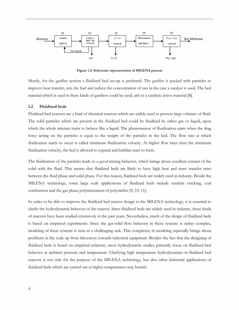
Approximately ten years ago, the Energy research Centre of the Netherlands (ECN) developed a technology
to produce bio-methane out of woody biomass. At the moment, the so called MILENA gasification
technology can produce bio-methane on a large scale. The MILENA process basically consists of five steps,
which are illustrated in Figure 1.3 [7]. The first step in this process is the gasification of biomass into a
producer gas. Subsequently, in the second and third step, the gas will be cooled, cleaned and any pollutants
will be removed. In the fourth step the producer gas will be transformed catalytically into CH4, CO2 and
H2O. The final step is the removal of the water and carbon dioxide and the compressing of the gas.
Figure 1.1: Ecological footprints of different biofuels compared to fossil fuels
Figure 1.2: Different routes for methane conversion
4
Figure 1.3: Schematic representation of MILENA process
Mostly, for the gasifier section a fluidized bed set-up is preferred. The gasifier is packed with particles to
improve heat transfer, mix the fuel and reduce the concentration of tars in the case a catalyst is used. The bed
material which is used in these kinds of gasifiers could be sand, ash or a catalytic active material [8].
1.2 Fluidized beds
Fluidized bed reactors are a kind of chemical reactors which are widely used to process large volumes of fluid.
The solid particles which are present in the fluidized bed could be fluidized by either gas or liquid, upon
which the whole mixture starts to behave like a liquid. The phenomenon of fluidization starts when the drag
force acting on the particles is equal to the weight of the particles in the bed. The flow rate at which
fluidization starts to occur is called minimum fluidization velocity. At higher flow rates than the minimum
fluidization velocity, the bed is allowed to expand and bubbles start to form.
The fluidization of the particles leads to a good mixing behavior, which brings about excellent contact of the
solid with the fluid. This means that fluidized beds are likely to have high heat and mass transfer rates
between the fluid phase and solid phase. For this reason, fluidized beds are widely used in industry. Beside the
MILENA technology, some large scale applications of fluidized beds include catalytic cracking, coal
combustion and the gas phase polymerization of polyolefins [9, 10, 11].
In order to be able to improve the fluidized bed reactor design in the MILENA technology, it is essential to
clarify the hydrodynamic behavior of the reactor. Since fluidized beds are widely used in industry, these kinds
of reactors have been studied extensively in the past years. Nevertheless, much of the design of fluidized beds
is based on empirical experiments. Since the gas-solid flow behavior in these systems is rather complex,
modeling of these systems is seen as a challenging task. This complexity in modeling especially brings about
problems in the scale up from laboratory towards industrial equipment. Besides the fact that the designing of
fluidized beds is based on empirical relations, most hydrodynamic studies primarily focus on fluidized bed
behavior at ambient pressure and temperature. Clarifying high temperature hydrodynamics in fluidized bed
reactors is not only for the purpose of the MILENA technology, but also other industrial applications of
fluidized beds which are carried out at higher temperatures may benefit.

Introduction
5
1.3 Temperature effects on hydrodynamics
Regardless the lacking number of publications on the influence of temperature on the fluidized bed
hydrodynamics, there is no complete agreement on the exact effects of temperature on the hydrodynamics.
According to Kunii and Levenspiel there are still contradictions regarding the reported findings, however,
these can be summarized as follows [12]:
- The porosity at minimum fluidization increases with temperature for fine particles. However, for
coarse particles, the porosity at minimum fluidization seems to be unaffected by temperature.
- For ambient temperature as well as for elevated temperatures, minimum fluidization velocity can be
reasonably well predicted by the dimensionless Ergun equation when the correct value for the
porosity at minimum fluidization is used:
( 1.1 )
in which the Archimedes number is given as:
( 1.2 )
and the Reynolds number as:
( 1.3 )
- Besides, increased temperatures bring about changes in bed behavior. For Geldart A classified
particles, bubble frequency increases with increasing temperature, as well as a significant decrease in
bubble size and a much smoother fluidization. Geldart B particles have a constant or somewhat
smaller bubble size and an enlarged region of good fluidization at higher temperatures. Geldart D
particles appear to have a constant or larger bubble size at increased temperatures.
In order to investigate the hydrodynamics of fluidized beds at higher temperatures, Sanaei et al. carried out
experiments with the radioactive particle tracking (RPT) technique [13]. They found that raising the
temperature from ambient to 300 °C shows an increase in emulsion phase velocity with an increase in
temperature. However, a decrease in emulsion phase velocities could be observed by a further increase in
temperature. This phenomenon is explained by the decrease in gas density and increase in gas viscosity at
elevated temperatures, which makes the drag force to increase after it initially decreased. This theory was
supported by an study performed by Choi et al. who used pressure fluctuation to describe the particle fluxes
in the fluidized bed at different gas velocities [14].

6
In a work published by Guo et al. the minimum fluidization velocities of different sized ash particles with a
Geldart B classification were determined at different temperatures, ranging from ambient up to 1000 °C [15].
The trend which was observed for the ash particles was that the minimum fluidization velocity decreased with
an increasing temperature. These observations are in accordance with work published by Svoboda and
Hartman, who studied the fluidization behavior of corundum, lime, brown coal ash and limestone at
temperatures ranging from 20 °C up to 890 °C [16]. In their work they described correlations to correct for
both density and viscosity change of air as a function of temperature (in K):
( 1.4 )
( 1.5 )
To describe the hydrodynamics of a fluidized bed reactor at different temperatures and superficial gas
velocities Cui et al. developed a high temperature optical fiber probe [17]. For their research they used
Geldart A classified particles which they tested in a temperature range from 25 °C up to 420 °C. It was found
that the particle concentration in both emulsion and bubble phase decreased with increasing temperature. The
changes in particle concentration cannot be explained by changes in density and viscosity changes as an effect
of increased temperature. Since not all changes in hydrodynamics observed in the research by Cui et al. can be
described by macro-scale changes, it is most likely that changes on micro-scale, such as interparticle forces are
playing a role at elevated temperatures [17].
Formisani et al. reported that higher temperatures could indeed cause an increase in interparticle forces,
which would influence the dynamic behavior in fluidized beds [18]. They demonstrated a clear change in
emulsion phase porosity, dense phase velocity and bubble hold-up with increasing the temperature up to 700
°C. It was observed that the dense phase porosity increased linearly with increasing temperature. However,
the rate of increasing of the dense phase porosity is smaller for particles with a higher density. Additionally,
other researchers state that interparticle forces between smaller particles are more influenced by temperature
than larger particles [19, 20].
Although more authors refer to changing interparticle forces playing a role on the hydrodynamics in fluidized
beds at elevated temperatures, the nature of this phenomenon still seems uncertain [21, 22, 23]. Massimillia
and Donsi ascribe the changes in interparticle forces at higher temperatures to changes in van der Waals
forces [24]. However, strong evidence is not given.
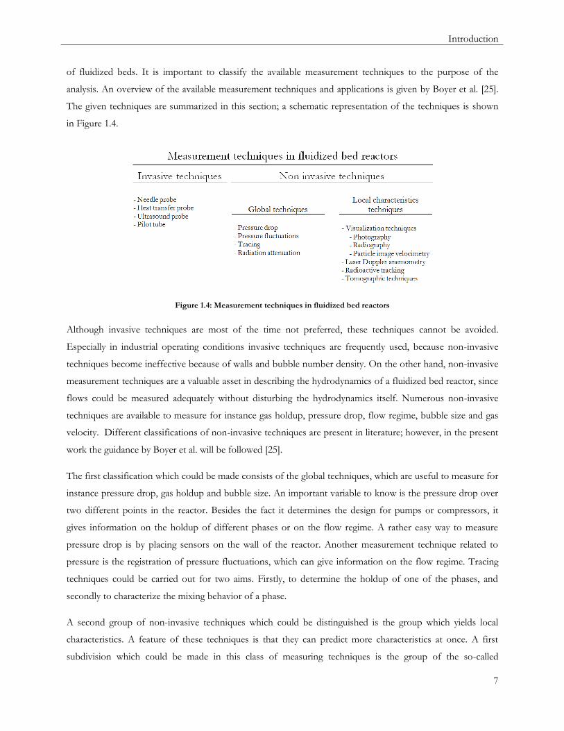
1.4 Measurement techniques
In general, a distinction between two different kinds of measurement techniques in fluidized beds can be
made. Both invasive as well as non-invasive techniques are used to obtain information on the hydrodynamics
Introduction
7
of fluidized beds. It is important to classify the available measurement techniques to the purpose of the
analysis. An overview of the available measurement techniques and applications is given by Boyer et al. [25].
The given techniques are summarized in this section; a schematic representation of the techniques is shown
in Figure 1.4.
Figure 1.4: Measurement techniques in fluidized bed reactors
Although invasive techniques are most of the time not preferred, these techniques cannot be avoided.
Especially in industrial operating conditions invasive techniques are frequently used, because non-invasive
techniques become ineffective because of walls and bubble number density. On the other hand, non-invasive
measurement techniques are a valuable asset in describing the hydrodynamics of a fluidized bed reactor, since
flows could be measured adequately without disturbing the hydrodynamics itself. Numerous non-invasive
techniques are available to measure for instance gas holdup, pressure drop, flow regime, bubble size and gas
velocity. Different classifications of non-invasive techniques are present in literature; however, in the present
work the guidance by Boyer et al. will be followed [25].
The first classification which could be made consists of the global techniques, which are useful to measure for
instance pressure drop, gas holdup and bubble size. An important variable to know is the pressure drop over
two different points in the reactor. Besides the fact it determines the design for pumps or compressors, it
gives information on the holdup of different phases or on the flow regime. A rather easy way to measure
pressure drop is by placing sensors on the wall of the reactor. Another measurement technique related to
pressure is the registration of pressure fluctuations, which can give information on the flow regime. Tracing
techniques could be carried out for two aims. Firstly, to determine the holdup of one of the phases, and
secondly to characterize the mixing behavior of a phase.
A second group of non-invasive techniques which could be distinguished is the group which yields local
characteristics. A feature of these techniques is that they can predict more characteristics at once. A first
subdivision which could be made in this class of measuring techniques is the group of the so-called
8
visualization techniques. These techniques result in knowledge on bubble shape and size. Besides
visualization techniques, Laser Doppler anemometry is part of the local characteristics group as well. This
technique is, not surprisingly, based on the Doppler effect, which could be described as a shift in frequency
between wave source and receiver. At last, tomography is a powerful tool to get information on the phase
fraction distribution inside the reactor. The principle of this technique is based on the measurement of a
physical property which can be related to the phase fraction in the column.
1.5 Particle image velocimetry coupled with digital image analysis
As indicated in Section 1.4, particle image velocimetry (PIV) could be used in order to investigate
hydrodynamics of fluidized bed reactors. PIV could be seen as a rather new analytical tool, since the first
article reporting on PIV appeared some 30 years ago [26]. A modern definition of PIV is given by Adrian: the
accurate, quantitative measurement of fluid velocity vectors at very large number of point simultaneously [27].
The vectors could be obtained by recording images of particles or patterns at two or more precisely defined
times.
In PIV, recorded double frame images are split into a large number of interrogation areas [28]. The
displacement of the interrogation areas could be calculated by cross correlating the interrogation area of both
images. The cross correlation produces a signal peak, which indentifies the displacement with respect to both
images. In order to obtain a velocity vector map, cross-correlation is repeated for all interrogation areas.
Laverman et al. reported on a phenomenon called particle raining, which could not be accounted for using
PIV [29]. Particle raining is characterized by a small amount of particles in the bubble phase, having a very
high velocity, while the particle mass flux is small. If the high velocities in the bubble phase are not corrected
for, this will eventually lead to errors in the average mass fluxes, since the mass flux is the product of the
porosity and velocity. Time averaged mass fluxes are of major importance while these results are the only
results which could be compared to each other since velocities are never similar. Digital image analysis (DIA)
could be used to distinguish between the bubble and the emulsion phase. The main characteristic of DIA is
to relate the pixel intensity to one of the phases. Usually, a certain threshold intensity is used to assign a
certain pixel to the bubble or to the emulsion phase. With the assumption that there are no particles present
in the bubble and that the emulsion phase density is constant, the average emulsion phase fraction could be
determined.
Different steps and algorithms could be distinguished in the DIA principle [29]. Firstly, the digital image is
imported and normalized. Next, an algorithm is used to detect the edges of the picture, so walls can be
removed. To correct for inhomogeneous illumination, the algorithm determines the local average intensity
and subtracts this from the original image. Finally, the noise is removed from the image, which will eventually
lead to a picture which clearly shows the phase separation of the emulsion and bubble phases.
Introduction
9
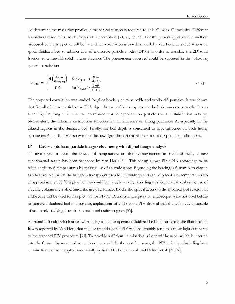
To determine the mass flux profiles, a proper correlation is required to link 2D with 3D porosity. Different
researchers made effort to develop such a correlation [30, 31, 32, 33]. For the present application, a method
proposed by De Jong et al. will be used. Their correlation is based on work by Van Buijtenen et al. who used
spout fluidized bed simulation data of a discrete particle model (DPM) in order to translate the 2D solid
fraction to a true 3D solid volume fraction. The phenomena observed could be captured in the following
general correlation:
( 1.6 )
The proposed correlation was studied for glass beads, γ-alumina oxide and zeolite 4A particles. It was shown
that for all of these particles the DIA algorithm was able to capture the bed phenomena correctly. It was
found by De Jong et al. that the correlation was independent on particle size and fluidization velocity.
Nonetheless, the intensity distribution function has an influence on fitting parameter A, especially in the
diluted regions in the fluidized bed. Finally, the bed depth is concerned to have influence on both fitting
parameters A and B. It was shown that the new algorithm decreased the error in the predicted solid fluxes.
1.6 Endoscopic laser particle image velocimetry with digital image analysis
To investigate in detail the effects of temperature on the hydrodynamics of fluidized beds, a new
experimental set-up has been proposed by Van Heck [34]. This set-up allows PIV/DIA recordings to be
taken at elevated temperatures by making use of an endoscope. Regarding the heating, a furnace was chosen
as a heat source. Inside the furnace a transparent pseudo 2D fluidized bed can be placed. For temperatures up
to approximately 500 °C a glass column could be used, however, exceeding this temperature makes the use of
a quartz column inevitable. Since the use of a furnace blocks the optical access to the fluidized bed reactor, an
endoscope will be used to take pictures for PIV/DIA analysis. Despite that endoscopes were not used before
to capture a fluidized bed in a furnace, applications of endoscopic PIV showed that the technique is capable
of accurately studying flows in internal combustion engines [35].
A second difficulty which arises when using a high temperature fluidized bed in a furnace is the illumination.
It was reported by Van Heck that the use of endoscopic PIV requires roughly ten times more light compared
to the standard PIV procedure [34]. To provide sufficient illumination, a laser will be used, which is inserted
into the furnace by means of an endoscope as well. In the past few years, the PIV technique including laser
illumination has been applied successfully by both Dierkshelde et al. and Delnoij et al. [35, 36].
10
1.7 State of the art
The work done by Van Heck could be characterized as preliminary work on the proposed set-up by selecting
the proper materials and equipment [34]. Besides, a new DIA algorithm was developed which is suitable for
the proposed purposes. Based on DPM simulations, the bubble detection algorithm by De Jong et al. has
been implemented (Equation 1.6). As a final part of his research Van Heck made a start with the validation of
the endoscopic laser PIV/DIA technique. As a benchmark, a cold flow pseudo 2D fluidized bed was used,
illuminated with LEDs. The column was packed with glass beads, since they are easily comparable to
literature data, for instance to De Jong et al. [33]. Experiments carried out with laser light as source of
illumination showed comparable time averaged flux profiles to the benchmark experiment. However, it
seemed that the position of the laser had some influence on the results. In addition, experiments carried out
with both laser illumination and an optical endoscope matched with the benchmark experiments.
One of the things Van Belzen investigated was the influence of the optical endoscope on the final results [37].
A possible effect of using an optical endoscope is barrel distortion. The effect of barrel distortion is that it
looks like a picture is mapped around a sphere. However, it was found that there is no need to correct for
barrel distortion, since it has minor influence on the actual results. As a result of the optical lens used, the
outer corners of the picture taken are sensitive to blurriness. In order to avoid the negative influences caused
by blurriness, the outer corners could be masked before processing the image. Another variable which was
tested by Van Belzen was the position of the laser. It was found that, for the current set-up, the angle
between the optical endoscope and the laser should be at least 25 °. At smaller angels, a reflection of the laser
light is visible on the pictures taken. At higher laser angels, the light intensity decreases. Furthermore, Van
Belzen estimated both the deviations in porosity and velocity. It was shown that the major part of the
deviations in the mass fluxes is caused by deviations in velocity. Finally, van Belzen ran experiments up to 200
°C to demonstrate the operability of the set-up and the capability of the technique to run PIV/DIA at
elevated temperatures

Experimental study on high temperature fluidization
11
2 Experimental study on high temperature fluidization
Unless the fact that industrial fluidized beds are commonly operated at high ratios of u0/umf, the minimum fluidization velocity
remains one of the critical design parameters. Up to now, most research on the minimum fluidization velocity has focused on
fluidization at room temperature and fluidization with common gases as air and nitrogen. Adversely, results on high temperature
fluidization which are available in literature are contradictive and can presently not been explained with the available knowledge
and correlations. In this part, high temperature fluidization will be investigated with different gases and particles, after which
possible parameters affecting high temperature fluidization will be examined.
12
2.1 Introduction
The hydrodynamics of fluidized beds depend on several factors such as solids properties, gas properties,
interparticle forces and reactor aspect ratio. These factors combined determine the value of the minimum
fluidization velocity (umf), which is mainly used for design purposes. Over the years, several correlations have
been reported on to predict the minimum fluidization velocity. However, most of these correlations are
correlated to experimental data obtained at room temperature. Nonetheless, some research has been done on
the temperature effects on minimum fluidization, but no common clarity could be found in literature.
It seems that the dependence of minimum fluidization velocity on temperature is affected not only by
temperature itself, but also by the nature and material of the particles. Increasing the temperature may cause
the minimum fluidization velocity to increase, to decrease or also to remain practically unvaried [38]. Pattipati
and Wen observed a decrease in the minimum fluidization velocity with increasing temperature for sand
particles with a diameter smaller than 2 mm with air as fluidizing medium [39]. On the other hand they found
an increase in minimum fluidization velocity with temperature for sand particles with a diameter larger than 2
mm. Practically at the same time Botterill et al. showed that for Geldart B particles the minimum fluidization
velocity decreased with increasing temperature [40]. For Geldart D particles it was found that the minimum
fluidization velocity increases with increasing temperature.
Results published by Rapagna et al. show that, for both particles which belong to the Geldart A as well as
particles which belong to the Geldart B classification, minimum fluidization velocity decreases with increasing
temperature [41]. However, it was shown that at higher temperatures the decrease is less than expected when
compared to the Ergun equation.
Xie and Geldart investigated the fluidization behavior of cracking catalyst particles which belong to the
Geldart A classification [42]. Besides for air, they determined the minimum fluidization velocity for argon,
neon, carbon dioxide and Freon-12. Just as Rapagna et al. they observed a decreasing trend of minimum
fluidization velocity with increasing temperature. They compared their experimental outcomes to three
predictive equations (Baeyens and Geldart [43], Wen and Yu [44] and the Carman-Kozeny equation) which
were commonly used and concluded that the minimum fluidization velocity could be predicted with an
accuracy of 50 % for all three correlations.
Most recently, Subramani et al. observed a decreasing trend of minimum fluidization velocity with increasing
temperature for different types of particles in the Geldart B classification [45].
Most of the correlations to predict minimum fluidization velocity reported in literature are based on the
Ergun equation. This equation, which was derived by Sabri Ergun in 1952, is based on the procedure to set

Experimental study on high temperature fluidization
13
the drag force of the gas equal to the weight force of the particles in the bed. In its original form, this
equation is used to predict the friction factor in a packed bed as a function of the Reynolds number:
( 2.1 )
where the friction factor could also be written as:
( 2.2 )
Figure 2.1 shows a representation of the Ergun equation. It could be seen that up to a Reynolds number of
10 the first term on the right hand side dominates. This term represents the pressure loss through viscous
effects, which is dominant in the laminar regime. At high Reynolds numbers (Re > 1000), the pressure loss
due to inertial forces is dominant. This means that the friction factor is constant in this regime.
The Ergun equation could be made dimensionless by realizing that the pressure drop over a packed bed is
equal to:
( 2.3 )
Rewriting and applying for minimum fluidization results in the following dimensionless equation which is
function of both the Reynolds number and Archimedes number:
( 2.4 )
Where the Reynolds number for minimum fluidization is given as:
( 2.5 )
and the Archimedes number as:
( 2.6 )
In many cases, the porosity at minimum fluidization and the shape factor of the particles is not known.
Therefore, Equation 2.4 could be rewritten in a more general form:
( 2.7 )
where
( 2.8 )

14
0.1
1
10
100
1000
10000
0.1 1 10 100 1000 10000 100000
f p[-
]
Re [-]
fp vs. Re
Figure 2.1: Visualization of Ergun equation
Figure 2.2: Constant C1 for a wide range of conditions
Figure 2.3: Constant C2 for a wide range of conditions

Experimental study on high temperature fluidization
15
It was noticed by Wen and Yu that C1 and C2 stayed nearly constant for different kinds of particles over a
wide range of conditions (Remf = 0.001 to 4 000) (Figure 2.2 and Figure 2.3) [46]. Wen and Yu compared 284
data points available in literature and concluded that C1 should be equal to approximately 14 and C2 to 11.
With the proposed constants, the minimum fluidization velocity could be predicted with a 34 % standard
deviation [44].
As indicated earlier, at Reynolds numbers smaller than 10, the pressure losses are mainly dominated by
viscous forces. In this case the pressure drop could be given by the so-called Carman-Kozeny equation,
which is a simplification of the Ergun equation for this specific regime:
( 2.9 )
Making use of Equation 2.3 and making dimensionless yields the following equation to predict the Reynolds
number at minimum fluidization:
( 2.10 )
Another common approach to predict minimum fluidization velocity which is found in literature is to
correlate experimental data for the Reynolds number at minimum fluidization to the Archimedes number in
the following way:
( 2.11 )
Various values for the empirical parameters a and b could be found, however, just as for the Wen and Yu type
of equations, most of them are determined at ambient conditions. An overview of the equations which are
present in literature and frequently used to determine the minimum fluidization velocity is given in
Table 2.1. For most of the equations reported, the type of particles and fluidization medium is given.
Based on the insights which are available in literature, predicting the minimum fluidization velocity at high
temperatures seems not to be straightforward. Most correlations which are used to predict the minimum
fluidization velocity are a simplification of the common used Ergun or Carman-Kozeny equations or of an
empirical nature. Therefore those equations cannot be used in a broad range of conditions, but are only
applicable to certain well-defined cases. Especially fluidization at high temperature seems to be a
phenomenon which is difficult to capture in the current predictive correlations. Besides, there is a lack of
research on fluidization with different gases than air or nitrogen. This part of this work will cover fluidization
experiments at high temperature with different gases. The results will be analyzed in order to be able to assign
possible parameters which influence fluidization at high temperature.

16
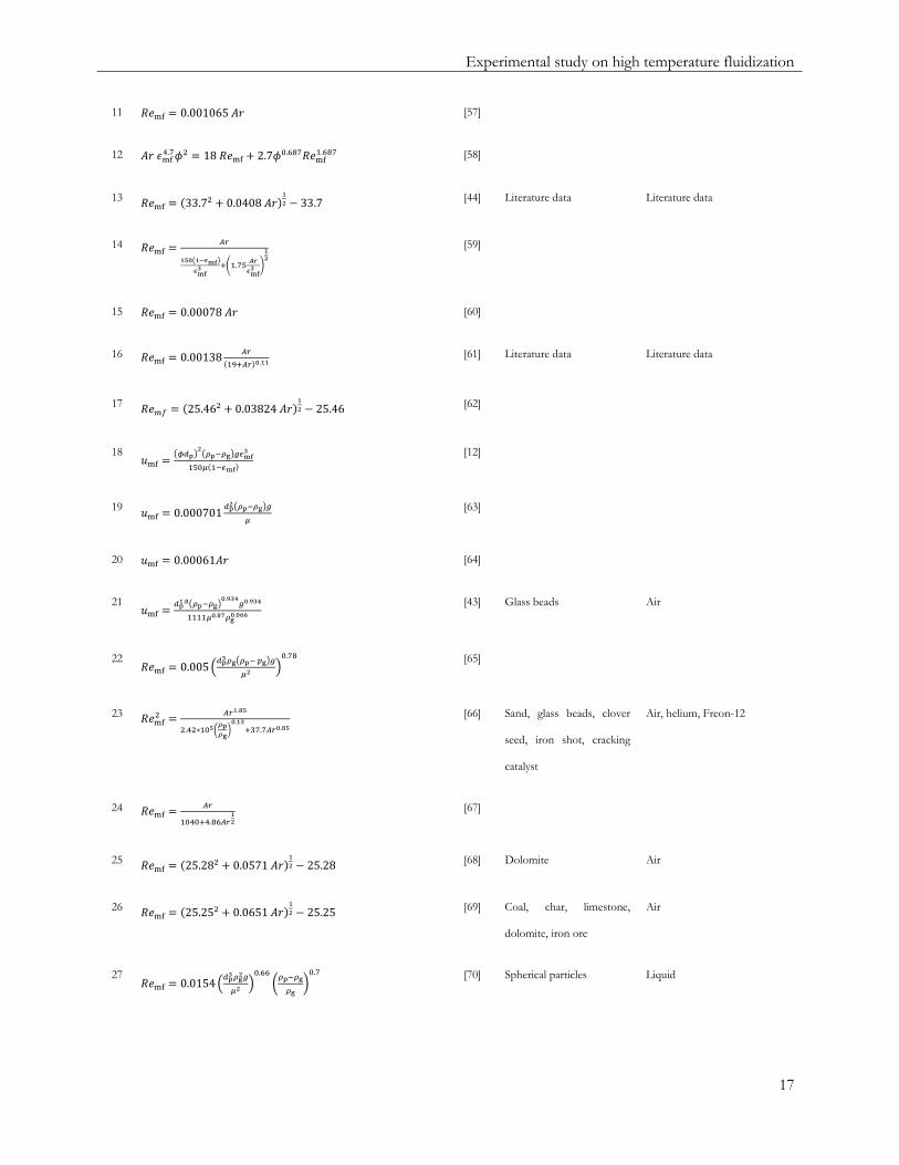
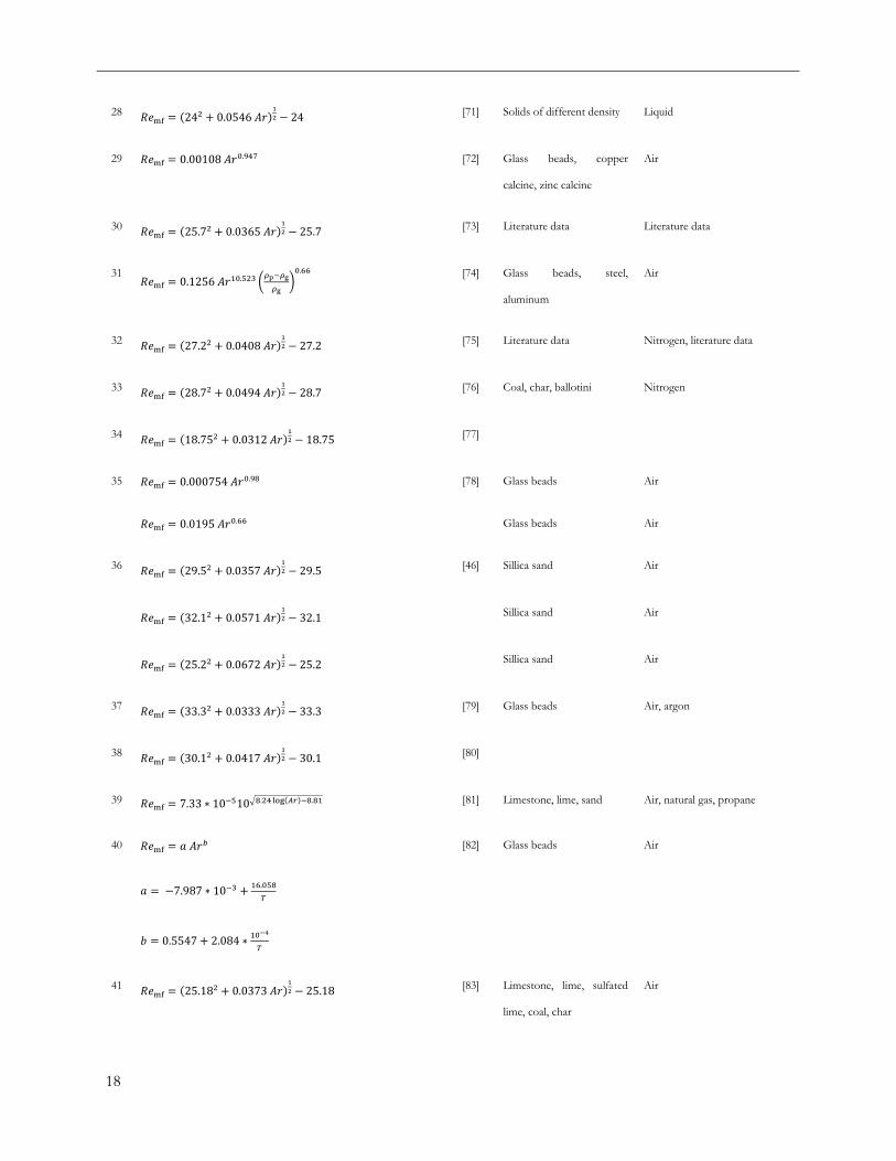
Table 2.1: Available literature correlations to predict minimum fluidization velocity
# Correlation Ref Particles Gases
1
[47]
2
[48] Silicon carbide, aluminum
oxide, silicon dioxide, silica
Air, helium, carbon
dioxide, ethane
3
[49] Carborundum, iron oxide
and coke
Air, argon, carbon dioxide,
nitrogen, town gas and
methane
4
[50]
5
[51] Sand, iron, silica gel Air, carbon dioxide,
nitrogen
6
[52]
7
[53] Sand, coal Air
[53] Sand, coal Air
8
[54] Glass beads, steel balls,
lead shot
Oil, water, glycerol-water
9 [55]
10
[56] Literature data Literature data
Experimental study on high temperature fluidization
17
11 [57]
12
[58]
13
[44] Literature data Literature data
14
[59]
15 [60]
16
[61] Literature data Literature data
17
[62]
18
[12]
19
[63]
20 [64]
21
[43] Glass beads Air
22
[65]
23
[66] Sand, glass beads, clover
seed, iron shot, cracking
catalyst
Air, helium, Freon-12
24
[67]
25
[68] Dolomite Air
26
[69] Coal, char, limestone,
dolomite, iron ore
Air
27
[70] Spherical particles Liquid
18
28
[71] Solids of different density Liquid
29 [72] Glass beads, copper
calcine, zinc calcine
Air
30
[73] Literature data Literature data
31
[74] Glass beads, steel,
aluminum
Air
32
[75] Literature data Nitrogen, literature data
33
[76] Coal, char, ballotini Nitrogen
34
[77]
35 [78] Glass beads Air
Glass beads Air
36
[46] Sillica sand Air
Sillica sand Air
Sillica sand Air
37
[79] Glass beads Air, argon
38
[80]
39 [81] Limestone, lime, sand Air, natural gas, propane
40
[82] Glass beads Air
41
[83] Limestone, lime, sulfated
lime, coal, char
Air

Experimental study on high temperature fluidization
19
Limestone, lime, sulfated
lime, coal, char
Air
42
[84] Sand and literature data Air
43 [85] Corn kernels, sand Air
44
[86] Polystyrene, tapioca, rice,
aluminum, salt, glass beads,
sand, corundum, corn
Air
Polystyrene, tapioca, rice,
aluminum, salt, glass beads,
sand, corundum, corn
Air
45
[87] Literature data Literature data
46
[42] FCC catalyst Air, argon, neon, carbon
dioxide, Freon-12
47 [88]
48 [89] Sand Air
Sand Air
49
[90] Wooden particles Air
50
[91] Dolomite, dolomite lime Air
Dolomite, dolomite lime Air
51
[92] Literature data Literature data
52
[93] Literature data Literature data
53
[94] Quartz sand, glass beads Air

20
54
[45] Ilmenite, sand, limestone,
quartz magnetite
Air
55 [95] Zirconium, glass beads,
iron, aluminum, sand, salt
Air
56
[96] Sand, glass beads, alumina,
wood
Air
57
[97] Literature data Literature data
2.2 Experimental procedure
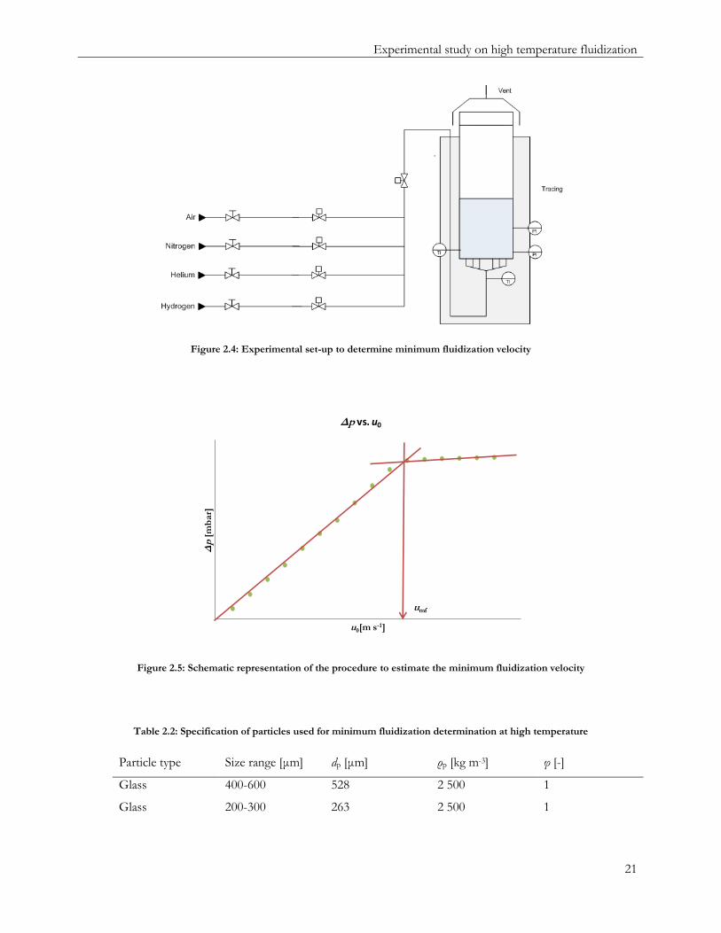
In order to determine the minimum fluidization at high temperatures, a set-up is used which is depicted in
Figure 2.4. This experimental set-up consists of a 50 cm long steel cylindrical tube with an inner diameter of
2.5 cm. A porous plate is used as gas distributor. The preheating of the gas and the reactor is achieved by an
internal tracer. The temperature of the tracer could be set by a thermocouple at the inlet of the reactor. The
true temperature of the gas entering the reactor could be measured by a thermocouple placed just above the
porous plate distributor. The pressure difference created by an increasing gas flow will be measured by two
SensorTechnics 26PC pressure transducers, reaching up to 50 mbar, which are connected to the reactor at a
known height above each other.
A known amount of particles is loaded into the reactor, which is then fluidized with nitrogen. Subsequently,
the tracer temperature is set to the desired temperature. After the reactor attains the desired steady state
temperature, the gas flow is switched off and thereafter increased with small steps in order to determine the
pressure difference at a certain gas flow. From a plot with the pressure difference as a function of the
superficial gas velocity, the minimum fluidization velocity could be obtained from the intersection of the
extrapolated line of the pressure drop across the bed and the line of the maximum theoretical pressure drop.
This procedure is visualized in Figure 2.5 and explained in detail in Appendix 1.
In this part of the research, two different sized glass beads will be used. Specifications of the glass beads used
are given in Table 2.2. Particle distributions and mean diameters have been determined with a Fritsch
Analysette 22 MicroTec plus laser particle sizer. As fluidization gases, besides air, nitrogen, helium and
hydrogen were used. Experiments were carried out at temperatures ranging from room temperature up to 500
°C. Corresponding gas density and viscosity were calculated according to the commonly used UNIQUAC
method. Figure 2.6 shows the density plotted as a function of viscosity for all those gases.
Experimental study on high temperature fluidization
21
Figure 2.4: Experimental set-up to determine minimum fluidization velocity
Δp
[mb
ar]
u0[m s-1]
Δp vs. u0
umf
Figure 2.5: Schematic representation of the procedure to estimate the minimum fluidization velocity
Table 2.2: Specification of particles used for minimum fluidization determination at high temperature
Particle type Size range [μm] dp [μm] ρp [kg m-3] φ [-]
Glass 400-600 528 2 500 1
Glass 200-300 263 2 500 1

22
0.0
0.2
0.4
0.6
0.8
1.0
1.2
1.4
0 0.005 0.01 0.015 0.02 0.025 0.03 0.035 0.04 0.045
ρg
[kg
m-3]
μ [10-3 Pa s]
ρ vs. μ
Air
N2
He
H2
Figure 2.6: Gas density as function of gas viscosity for air, nitrogen, helium and hydrogen. Markers placed at 25 °C, 50 °C,
100 °C, up to 500 °C
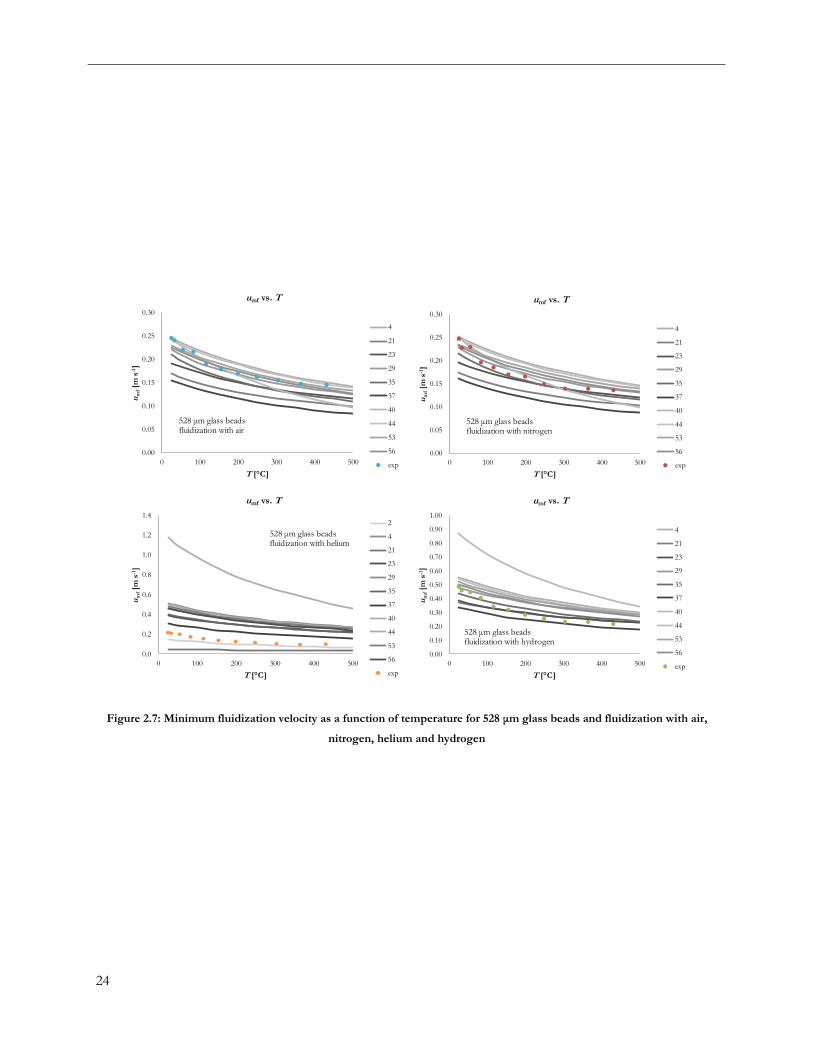
2.3 Results and discussion
The discussed procedure to determine the minimum fluidization velocity has been carried out for glass beads
of both the sizes 263 μm and 528 μm. The experimentally determined minimum fluidization velocities which
were obtained for the 528 μm glass beads are presented in Figure 2.7 as a function of temperature. Alongside
with the experimental values, the predicted values obtained from the correlations presented in
Table 2.1, corresponding to correlations for glass beads, have been plotted as well. The numbers presented in
the legend correspond with the numbers given in Table 2.1. As could be seen from the presented figures for
glass beads with a size of 528 μm for all the fluidization media, a decreasing trend of minimum fluidization
velocity could be observed with increasing temperature. This trend is in correspondence with the results
which were published earlier by Rapagna et al. and Subramani et al. for Geldart B particles [41, 45]. Besides, it
could be observed that the experimentally determined values for the minimum fluidization for 528 μm glass
beads fluidized with air and nitrogen fit reasonably well with the values predicted with the available
correlations in literature. However, for the fluidization media helium and hydrogen a severe underestimation
of the experimental data could be seen. It should be noted that most of the correlations reported in literature
are determined for experimental values of the minimum fluidization velocity with air as fluidizing medium.
Over the years, only two publications report on minimum fluidization velocity correlations obtained for
helium as a fluidization gas. The minimum fluidization velocities predicted for helium as a function of
temperature by the correlations proposed by Miller and Logwinuk (Correlation 2) and Broadhust and Becker
Experimental study on high temperature fluidization
23
(Correlation 23) have been added to Figure 2.7 [48, 66]. Unfortunately, no correlations for the prediction of
the minimum fluidization velocity for particles fluidized by hydrogen have been reported in literature.
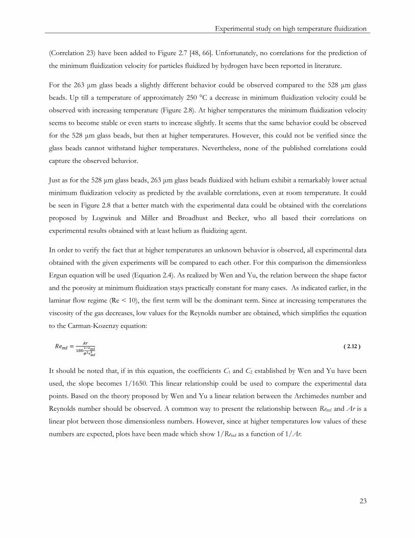
For the 263 μm glass beads a slightly different behavior could be observed compared to the 528 μm glass
beads. Up till a temperature of approximately 250 °C a decrease in minimum fluidization velocity could be
observed with increasing temperature (Figure 2.8). At higher temperatures the minimum fluidization velocity
seems to become stable or even starts to increase slightly. It seems that the same behavior could be observed
for the 528 μm glass beads, but then at higher temperatures. However, this could not be verified since the
glass beads cannot withstand higher temperatures. Nevertheless, none of the published correlations could
capture the observed behavior.
Just as for the 528 μm glass beads, 263 μm glass beads fluidized with helium exhibit a remarkably lower actual
minimum fluidization velocity as predicted by the available correlations, even at room temperature. It could
be seen in Figure 2.8 that a better match with the experimental data could be obtained with the correlations
proposed by Logwinuk and Miller and Broadhust and Becker, who all based their correlations on
experimental results obtained with at least helium as fluidizing agent.
In order to verify the fact that at higher temperatures an unknown behavior is observed, all experimental data
obtained with the given experiments will be compared to each other. For this comparison the dimensionless
Ergun equation will be used (Equation 2.4). As realized by Wen and Yu, the relation between the shape factor
and the porosity at minimum fluidization stays practically constant for many cases. As indicated earlier, in the
laminar flow regime (Re < 10), the first term will be the dominant term. Since at increasing temperatures the
viscosity of the gas decreases, low values for the Reynolds number are obtained, which simplifies the equation
to the Carman-Kozenzy equation:
( 2.12 )
It should be noted that, if in this equation, the coefficients C1 and C2 established by Wen and Yu have been
used, the slope becomes 1/1650. This linear relationship could be used to compare the experimental data
points. Based on the theory proposed by Wen and Yu a linear relation between the Archimedes number and
Reynolds number should be observed. A common way to present the relationship between Remf and Ar is a
linear plot between those dimensionless numbers. However, since at higher temperatures low values of these
numbers are expected, plots have been made which show 1/Remf as a function of 1/Ar.
24
0.00
0.05
0.10
0.15
0.20
0.25
0.30
0 100 200 300 400 500
um
f[m
s-1
]
T [°C]
umf vs. T
4
21
23
29
35
37
40
44
53
56
exp
528 μm glass beads fluidization with air
0.00
0.05
0.10
0.15
0.20
0.25
0.30
0 100 200 300 400 500
um
f[m
s-1
]
T [°C]
umf vs. T
4
21
23
29
35
37
40
44
53
56
exp
528 μm glass beads fluidization with nitrogen
0.0
0.2
0.4
0.6
0.8
1.0
1.2
1.4
0 100 200 300 400 500
um
f[m
s-1
]
T [°C]
umf vs. T
2
4
21
23
29
35
37
40
44
53
56
exp
528 μm glass beads fluidization with helium
0.00
0.10
0.20
0.30
0.40
0.50
0.60
0.70
0.80
0.90
1.00
0 100 200 300 400 500
um
f[m
s-1
]
T [°C]
umf vs. T
4
21
23
29
35
37
40
44
53
56
exp
528 μm glass beads fluidization with hydrogen
Figure 2.7: Minimum fluidization velocity as a function of temperature for 528 μm glass beads and fluidization with air,
nitrogen, helium and hydrogen

Experimental study on high temperature fluidization
25
0.00
0.02
0.04
0.06
0.08
0.10
0.12
0.14
0.16
0.18
0 100 200 300 400 500
um
f[m
s-1]
T [°C]
umf vs. T
4
21
23
29
35
37
40
44
53
56
exp
263 μm glass beads fluidization with air
0.00
0.02
0.04
0.06
0.08
0.10
0.12
0.14
0.16
0.18
0 100 200 300 400 500
um
f[m
s-1
]
T [°C]
umf vs. T
4
21
23
29
35
37
40
44
53
56
exp
263 μm glass beads fluidization with nitrogen
0.00
0.01
0.02
0.03
0.04
0.05
0.06
0.07
0 100 200 300 400 500
um
f[m
s-1]
T [°C]
umf vs. T
2
4
21
23
29
35
37
44
53
56
exp
263 μm glass beads fluidization with helium
0.00
0.02
0.04
0.06
0.08
0.10
0.12
0.14
0.16
0.18
0 100 200 300 400 500
um
f[m
s-1
]
T [°C]
umf vs. T
4
21
23
29
35
37
44
53
56
exp
263 μm glass beads fluidization with hydrogen
Figure 2.8: Minimum fluidization velocity as a function of temperature for 263 μm glass beads and fluidization with air,
nitrogen, helium and hydrogen
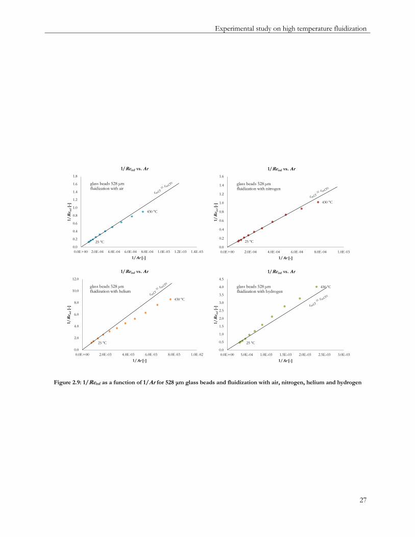
26
For the glass beads of 528 μm an almost clear linear relation between 1/Remf and 1/Ar could be observed for
fluidization with all gases (Figure 2.9). However, at higher temperatures, deviations from this linear relation
could be observed. For the 263 μm glass beads a linear relation could be seen for relatively high Reynolds and
Archimedes numbers (low temperatures), however, at lower values of these dimensionless numbers (higher
temperatures) deviations from the linear trend are observed (Figure 2.10).
The change in slope in the curves shown in Figure 2.9 and Figure 2.10 could be explained by a change in
porosity at minimum fluidization. As could be seen in Equation 2.12 is the slope a function of both sphericity
and porosity at minimum fluidization. Since the sphericity of the particles is assumed to be equal to unity for
all cases, a change in slope could be explained by a change in porosity at minimum fluidization. It was shown
that for the 263 μm glass beads the slope in a 1/Remf as a function of 1/Ar curve decreases with decreasing
Reynolds number and Archimedes number, and so with increasing temperature. A decrease in slope means
that, based on Equation 2.12, the porosity at minimum fluidization should increase. In these figures, a linear
trend line has been added to visualize the effect if the porosity at minimum fluidization at room temperature
is accepted for elevated temperatures as well.
2.4 Conclusions
Over the years, quite some research groups put effort in investigating the minimum fluidization behavior of
fine particles. Up to now, no accordance has been reached in open literature. Unless the fact that it seems that
fluidization at room temperature and with air as fluidization gas is understood, high temperature fluidization
still seems to be a mystery. For Geldart B classified particles, there seems consensus that at higher
temperatures, the minimum fluidization velocity is lower that at room temperature. However, compared to
well-accepted correlations, the minimum fluidization velocity seems higher than expected. Besides,
fluidization with gases different than air, or nitrogen, seems to give additional problems.
In this part of the research, a first step has been made in order to find possible reasons why high temperature
fluidization is so hard to explain. For different particles and gases, results were found which were in
accordance with literature. Analyses of the results lead to the presumption that the porosity at minimum
fluidization, which is assumed to be constant in many cases, is subject to change for different particle and gas
properties and temperature.
Experimental study on high temperature fluidization
27
25 °C
430 °C
0.0
0.2
0.4
0.6
0.8
1.0
1.2
1.4
1.6
1.8
0.0E+00 2.0E-04 4.0E-04 6.0E-04 8.0E-04 1.0E-03 1.2E-03 1.4E-03
1/R
em
f[-
]
1/Ar [-]
1/Remf vs. Ar
glass beads 528 μmfluidization with air
25 °C
430 °C
0.0
0.2
0.4
0.6
0.8
1.0
1.2
1.4
1.6
0.0E+00 2.0E-04 4.0E-04 6.0E-04 8.0E-04 1.0E-03
1/R
em
f[-
]
1/Ar [-]
1/Remf vs. Ar
glass beads 528 μmfluidization with nitrogen
25 °C
430 °C
0.0
2.0
4.0
6.0
8.0
10.0
12.0
0.0E+00 2.0E-03 4.0E-03 6.0E-03 8.0E-03 1.0E-02
1/R
em
f[-
]
1/Ar [-]
1/Remf vs. Ar
glass beads 528 μmfluidization with helium
25 °C
430 °C
0.0
0.5
1.0
1.5
2.0
2.5
3.0
3.5
4.0
4.5
0.0E+00 5.0E-04 1.0E-03 1.5E-03 2.0E-03 2.5E-03 3.0E-03
1/R
em
f[-
]
1/Ar [-]
1/Remf vs. Ar
glass beads 528 μmfluidization with hydrogen
Figure 2.9: 1/Remf as a function of 1/Ar for 528 μm glass beads and fluidization with air, nitrogen, helium and hydrogen

28
25 °C
430 °C
0.0
1.0
2.0
3.0
4.0
5.0
6.0
7.0
8.0
9.0
10.0
0.0E+00 1.0E-03 2.0E-03 3.0E-03 4.0E-03 5.0E-03 6.0E-03 7.0E-03
1/R
em
f[-
]
1/Ar [-]
1/Remf vs. Ar
glass beads 263 μmfluidization with air
25 °C
430 °C
0.0
2.0
4.0
6.0
8.0
10.0
12.0
0.0E+00 2.0E-03 4.0E-03 6.0E-03 8.0E-03 1.0E-02
1/R
em
f[-
]
1/Ar [-]
1/Remf vs. Ar
glass beads 263 μmfluidization with nitrogen
25 °C
430 °C
0.0
20.0
40.0
60.0
80.0
100.0
120.0
140.0
0.0E+00 1.0E-02 2.0E-02 3.0E-02 4.0E-02 5.0E-02 6.0E-02 7.0E-02
1/R
em
f[-
]
1/Ar [-]
1/Remf vs. Ar
glass beads 263 μmfluidization with helium
25 °C
430 °C
0.0
5.0
10.0
15.0
20.0
25.0
30.0
0.0E+00 5.0E-03 1.0E-02 1.5E-02 2.0E-02 2.5E-02
1/R
em
f[-
]
1/Ar [-]
1/Remf vs. Ar
glass beads 263 μmfluidization with hydrogen
Figure 2.10: 1/Remf as a function of 1/Ar for 263 μm glass beads and fluidization with air, nitrogen, helium and hydrogen

Experimental study on the porosity at minimum fluidization
29
3 Experimental study on the porosity at minimum fluidization
A well-accepted procedure to predict the minimum fluidization velocity is to assume a constant porosity at minimum fluidization
(εmf). However, new insights show that this assumption might not be valid. Besides, a slight difference in porosity at minimum
fluidization could result in a severe error in the prediction of the minimum fluidization velocity. In literature no clarification was
given on the possible parameters influencing the porosity at minimum fluidization. Therefore, in this section the influence of
particle and gas properties and temperature has been studied on the porosity at minimum fluidization. As a result, it was found
that particle size and shape, as well as gas density and temperature have an influence on the porosity at minimum fluidization.
Regression analysis on these variables shows that the porosity at minimum fluidization could be predicted with a maximum error
of 3 %, which results in a prediction of umf within an error of 10 %.
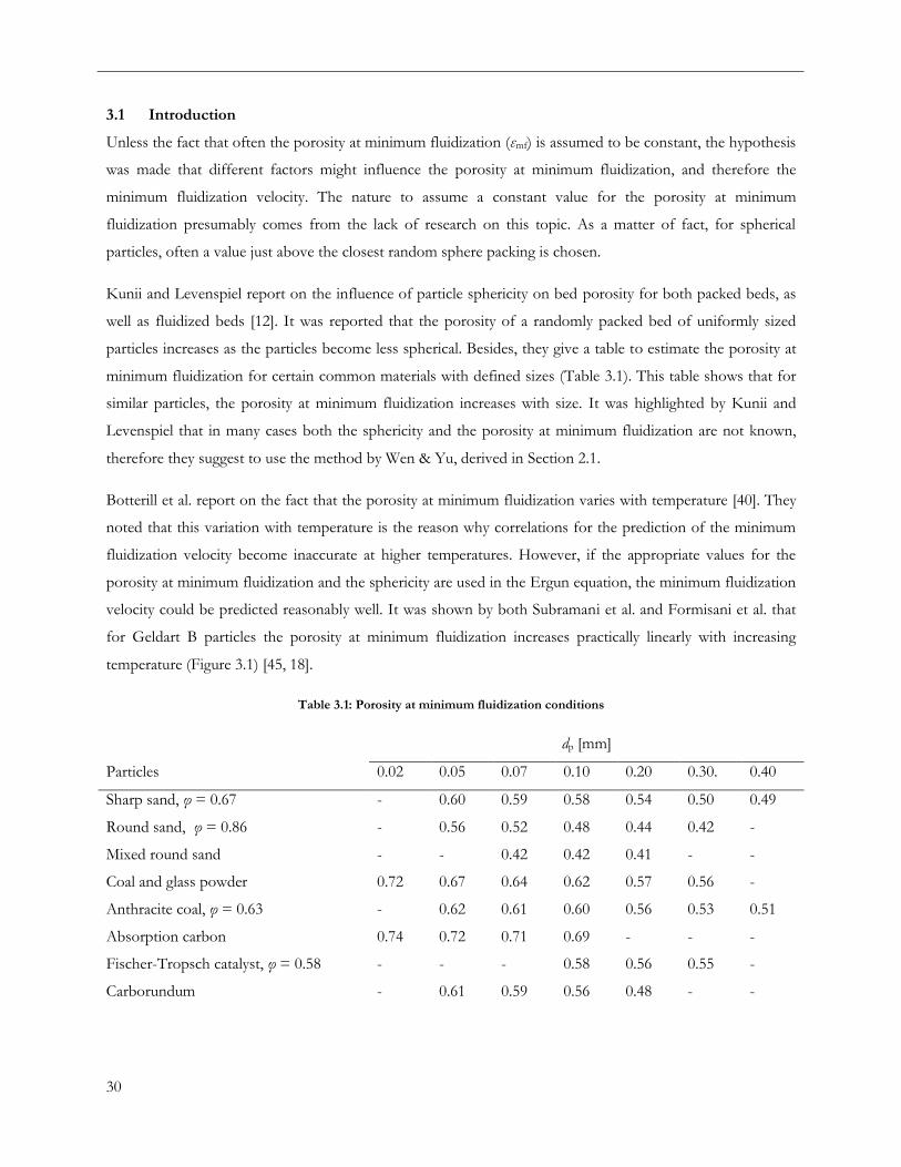
30
3.1 Introduction
Unless the fact that often the porosity at minimum fluidization (εmf) is assumed to be constant, the hypothesis
was made that different factors might influence the porosity at minimum fluidization, and therefore the
minimum fluidization velocity. The nature to assume a constant value for the porosity at minimum
fluidization presumably comes from the lack of research on this topic. As a matter of fact, for spherical
particles, often a value just above the closest random sphere packing is chosen.
Kunii and Levenspiel report on the influence of particle sphericity on bed porosity for both packed beds, as
well as fluidized beds [12]. It was reported that the porosity of a randomly packed bed of uniformly sized
particles increases as the particles become less spherical. Besides, they give a table to estimate the porosity at
minimum fluidization for certain common materials with defined sizes (Table 3.1). This table shows that for
similar particles, the porosity at minimum fluidization increases with size. It was highlighted by Kunii and
Levenspiel that in many cases both the sphericity and the porosity at minimum fluidization are not known,
therefore they suggest to use the method by Wen & Yu, derived in Section 2.1.
Botterill et al. report on the fact that the porosity at minimum fluidization varies with temperature [40]. They
noted that this variation with temperature is the reason why correlations for the prediction of the minimum
fluidization velocity become inaccurate at higher temperatures. However, if the appropriate values for the
porosity at minimum fluidization and the sphericity are used in the Ergun equation, the minimum fluidization
velocity could be predicted reasonably well. It was shown by both Subramani et al. and Formisani et al. that
for Geldart B particles the porosity at minimum fluidization increases practically linearly with increasing
temperature (Figure 3.1) [45, 18].
Table 3.1: Porosity at minimum fluidization conditions
dp [mm]
Particles 0.02 0.05 0.07 0.10 0.20 0.30. 0.40
Sharp sand, φ = 0.67 - 0.60 0.59 0.58 0.54 0.50 0.49
Round sand, φ = 0.86 - 0.56 0.52 0.48 0.44 0.42 -
Mixed round sand - - 0.42 0.42 0.41 - -
Coal and glass powder 0.72 0.67 0.64 0.62 0.57 0.56 -
Anthracite coal, φ = 0.63 - 0.62 0.61 0.60 0.56 0.53 0.51
Absorption carbon 0.74 0.72 0.71 0.69 - - -
Fischer-Tropsch catalyst, φ = 0.58 - - - 0.58 0.56 0.55 -
Carborundum - 0.61 0.59 0.56 0.48 - -

Experimental study on the porosity at minimum fluidization
31
Figure 3.1: Porosity at minimum fluidization as a function of temperature as established by a) Subramani et al. and b)
Formisani et al.
Correlations for the porosity at minimum fluidization are limited in literature (Table 3.2). It seems even that
currently none of the reported correlations can capture a wide range of different conditions. At the moment,
none of them could be used to predict the porosity at minimum fluidization accurately. In order to be able to
predict the minimum fluidization velocity both at room and at higher temperatures within an acceptable
error, understanding is needed in how the porosity at minimum fluidization depends on different variables.
In order to validate the available literature correlations, more than 100 data points from literature have been
evaluated (Appendix 2). These data points, which fall all in the Geldart B classification, have been used to
predict the porosity at minimum fluidization based on the correlations which are presented in Table 3.2.
These predicted values have been compared to the actual experimental values. Plots, which visualize these
comparisons, are shown in Figure 3.2. None of the available correlations seems successful in predicting the
actual porosity at minimum fluidization. However, both the correlation by Fatah and Subramani et al. show a
minimum value for the predicted porosity at minimum fluidization. Physically spoken, this value should be
just above the porosity related to the random closest sphere packing. In practise, this value would come close
to 0.40. It seems that both correlations over predict this minimum value for the porosity at minimum
fluidization. Besides, the correlation by Broadhurst and Becker seems physically incorrect, since it is capable
to predict values for the porosity at minimum fluidization which are far below the porosity related to the
random closest packing for spherical particles. It should be noted that these values appear at the largest
numbers for the Archimedes number. The authors are aware of this fact, but were not able to improve their
correlation.
Based on the available literature highlighted in this chapter and the experimental findings reported in the
previous chapter, possibly, the porosity at minimum fluidization will play a key role in predicting the
minimum fluidization velocity. Different researchers investigated the role of both the particle and gas

32
properties and temperature on the porosity at minimum fluidization independently, but none of them
combined those variables. Besides, the effort which was put into describing experimental data on the porosity
at minimum fluidization, has not lead to a common correlation yet.
Since the research which was done in the past sticks to the use of air as fluidizing medium, different fluidizing
gases and mixtures of gases will be used in this work. Making use of the gas mixtures allows investigating the
changes in gas density and viscosity at both room temperature and elevated temperatures. The goal of this
work would be to find out whether the porosity at minimum fluidization would be a key factor in predicting
the minimum fluidization velocity at different conditions. In order to verify the experimentally obtained
values for the porosity at minimum fluidization, these values are used to predict minimum fluidization
velocity by means of well-accepted relations by Ergun and Carman-Kozeny. Ultimately, the data obtained
shows a trend which could be described by an earlier published, or newly proposed, correlation to predict the
porosity at minimum fluidization.
3.2 Experimental procedure
A common approach to estimate the porosity at minimum fluidization makes use of pressure transducers. By
measuring the pressure drop over a certain height in the bed at different flow rates beyond the minimum
fluidization point, the average porosity of the reactor could be related in the following way (rewriting
Equation 2.3):
( 3.1 )
Table 3.2: Available literature correlations to predict porosity at minimum fluidization
# Correlation Ref Remark
1 [45] Reynolds number used to predict porosity at minimum
fluidization, only tested for air, sphericity not included
2
[66] Only tested at room temperature, physically incorrect for
higher values of Archimedes number
3
[82] Only tested at room temperature, sphericity not included
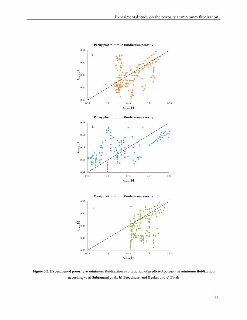
Experimental study on the porosity at minimum fluidization
33
0.35
0.40
0.45
0.50
0.55
0.35 0.40 0.45 0.50 0.55
ε mf,
exp[-
]
εmf,pred [-]
Parity plot minimun fluidization porostiy
a
0.35
0.40
0.45
0.50
0.55
0.35 0.40 0.45 0.50 0.55
ε mf,
exp
[-]
εmf,pred [-]
Parity plot minimun fluidization porosity
b
0.35
0.40
0.45
0.50
0.55
0.35 0.40 0.45 0.50 0.55
ε mf,
exp
[-]
εmf,pred [-]
Parity plot minimun fluidization porosity
c
Figure 3.2: Experimental porosity at minimum fluidization as a function of predicted porosity at minimum fluidization
according to a) Subramani et al., b) Broadhurst and Becker and c) Fatah

34
In order to estimate the porosity at minimum fluidization, the average porosity at different points beyond the
minimum fluidization velocity is determined. These values for the average porosity will give a linear fit with
respect to the flow rate. By extrapolating back to u0/umf = 1, one has access to the porosity at minimum
fluidization (Figure 3.3 and Appendix 3). This procedure has been carried out successfully by different
research groups in the past [45, 41, 20, 98, 40].
In this work, this procedure will be carried out both with measuring a pressure difference as well as with
digital image analysis (DIA). For the method including pressure transducers two SensorTechnics 26PC
pressure transducers will be used, ranging from 0 up to 50 mbar. Since the method involving DIA requires
optical access, a pseudo 2D fluidized bed set-up has been used. A schematic overview of this set-up is given
in Figure 3.4. By inserting a known weight of particles into the fluidized bed, the average bed porosity at a
certain flow rate can be related to the average bed height as follows:
( 3.2)
ε avg
[-]
u0/umf [-]
εavg vs. u0/umf
εmf
u0/umf = 1
Figure 3.3: Representation of the procedure to estimate the porosity at minimum fluidization
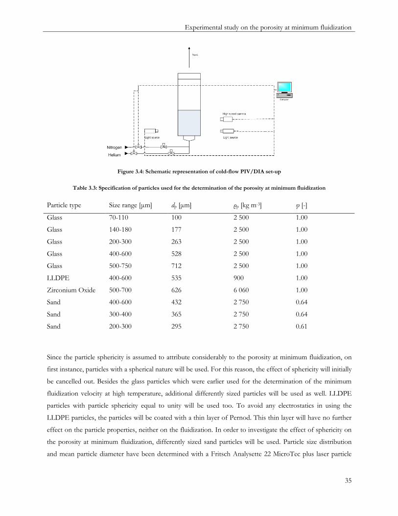
Experimental study on the porosity at minimum fluidization
35
Figure 3.4: Schematic representation of cold-flow PIV/DIA set-up
Table 3.3: Specification of particles used for the determination of the porosity at minimum fluidization
Particle type Size range [μm] dp [μm] ρp [kg m-3] φ [-]
Glass 70-110 100 2 500 1.00
Glass 140-180 177 2 500 1.00
Glass 200-300 263 2 500 1.00
Glass 400-600 528 2 500 1.00
Glass 500-750 712 2 500 1.00
LLDPE 400-600 535 900 1.00
Zirconium Oxide 500-700 626 6 060 1.00
Sand 400-600 432 2 750 0.64
Sand 300-400 365 2 750 0.64
Sand 200-300 295 2 750 0.61
Since the particle sphericity is assumed to attribute considerably to the porosity at minimum fluidization, on
first instance, particles with a spherical nature will be used. For this reason, the effect of sphericity will initially
be cancelled out. Besides the glass particles which were earlier used for the determination of the minimum
fluidization velocity at high temperature, additional differently sized particles will be used as well. LLDPE
particles with particle sphericity equal to unity will be used too. To avoid any electrostatics in using the
LLDPE particles, the particles will be coated with a thin layer of Pernod. This thin layer will have no further
effect on the particle properties, neither on the fluidization. In order to investigate the effect of sphericity on
the porosity at minimum fluidization, differently sized sand particles will be used. Particle size distribution
and mean particle diameter have been determined with a Fritsch Analysette 22 MicroTec plus laser particle

36
sizer. Particle sphericity has been determined with a CILAS ExpertShape particle analyzer. An overview of all
the particles and their properties is given in Table 3.3.
First, the porosity at minimum fluidization will be determined at room temperature for different particle
properties and gas properties. To create gases with different densities and viscosities, mixtures with different
ratios of helium and nitrogen will be used. Combining different gas mixtures with different particles generates
a broad range of different conditions.
As soon as the influences of the gas and particles properties on the porosity at minimum fluidization have
been established, temperature effects will be studied. For this part of the research, the reactor shown in
Figure 2.4 will be used. In order to investigate whether there is a combined effect of temperature and gas and
particles properties, two different gases or gas mixtures with the same density and viscosity at different
temperatures will be investigated. Since these gases have the same properties, and therefore the same
Archimedes number, one would expect the same Reynolds number at minimum fluidization, and therefore
the same porosity at minimum fluidization. For this investigation, a 0.19:0.81 mixture of neon and hydrogen
will be compared to pure helium. Figure 3.5 shows that, indeed, these gases have the same properties in a
defined region. As could been seen is that in a temperature range of helium from 25 °C up to 350 °C, gas
properties should correspond with the mixture in a range from 150 °C up to 500 °C. Gas properties have
been estimated with the UNIQUAC method.
50 °C
100 °C
150 °C
200 °C250 °C
300 °C350 °C
400 °C450 °C
500 °C
50 °C
100 °C
150 °C
200 °C
250 °C300 °C
350 °C400 °C
450 °C500 °C
0.0
0.1
0.2
0.3
0.010 0.015 0.020 0.025 0.030 0.035 0.040 0.045
ρg
[kg
m-3
]
μ [10-3 Pa s]
ρ vs. μ
Helium
0.19:0.81 Neon:Hydrogen
Figure 3.5: Gas density as function of gas viscosity for helium and 0.19:0.81 neon:hydrogen mixture. Markers placed every
50 °C
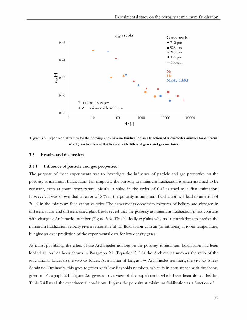
Experimental study on the porosity at minimum fluidization
37
0.38
0.40
0.42
0.44
0.46
1 10 100 1000 10000 100000
ε mf[-
]
Ar [-]
εmf vs. ArGlass beads● 712 μm
■ 528 μm
▲ 263 μm
♦ 177 μm
─ 100 μm
N2
He
N2:He 0.5:0.5
* LLDPE 535 μm
+ Zirconium oxide 626 μm
Figure 3.6: Experimental values for the porosity at minimum fluidization as a function of Archimedes number for different
sized glass beads and fluidization with different gases and gas mixtures
3.3 Results and discussion
3.3.1 Influence of particle and gas properties
The purpose of these experiments was to investigate the influence of particle and gas properties on the
porosity at minimum fluidization. For simplicity the porosity at minimum fluidization is often assumed to be
constant, even at room temperature. Mostly, a value in the order of 0.42 is used as a first estimation.
However, it was shown that an error of 5 % in the porosity at minimum fluidization will lead to an error of
20 % in the minimum fluidization velocity. The experiments done with mixtures of helium and nitrogen in
different ratios and different sized glass beads reveal that the porosity at minimum fluidization is not constant
with changing Archimedes number (Figure 3.6). This basically explains why most correlations to predict the
minimum fluidization velocity give a reasonable fit for fluidization with air (or nitrogen) at room temperature,
but give an over prediction of the experimental data for low density gases.
As a first possibility, the effect of the Archimedes number on the porosity at minimum fluidization had been
looked at. As has been shown in Paragraph 2.1 (Equation 2.6) is the Archimedes number the ratio of the
gravitational forces to the viscous forces. As a matter of fact, at low Archimedes numbers, the viscous forces
dominate. Ordinarily, this goes together with low Reynolds numbers, which is in consistence with the theory
given in Paragraph 2.1. Figure 3.6 gives an overview of the experiments which have been done. Besides,
Table 3.4 lists all the experimental conditions. It gives the porosity at minimum fluidization as a function of
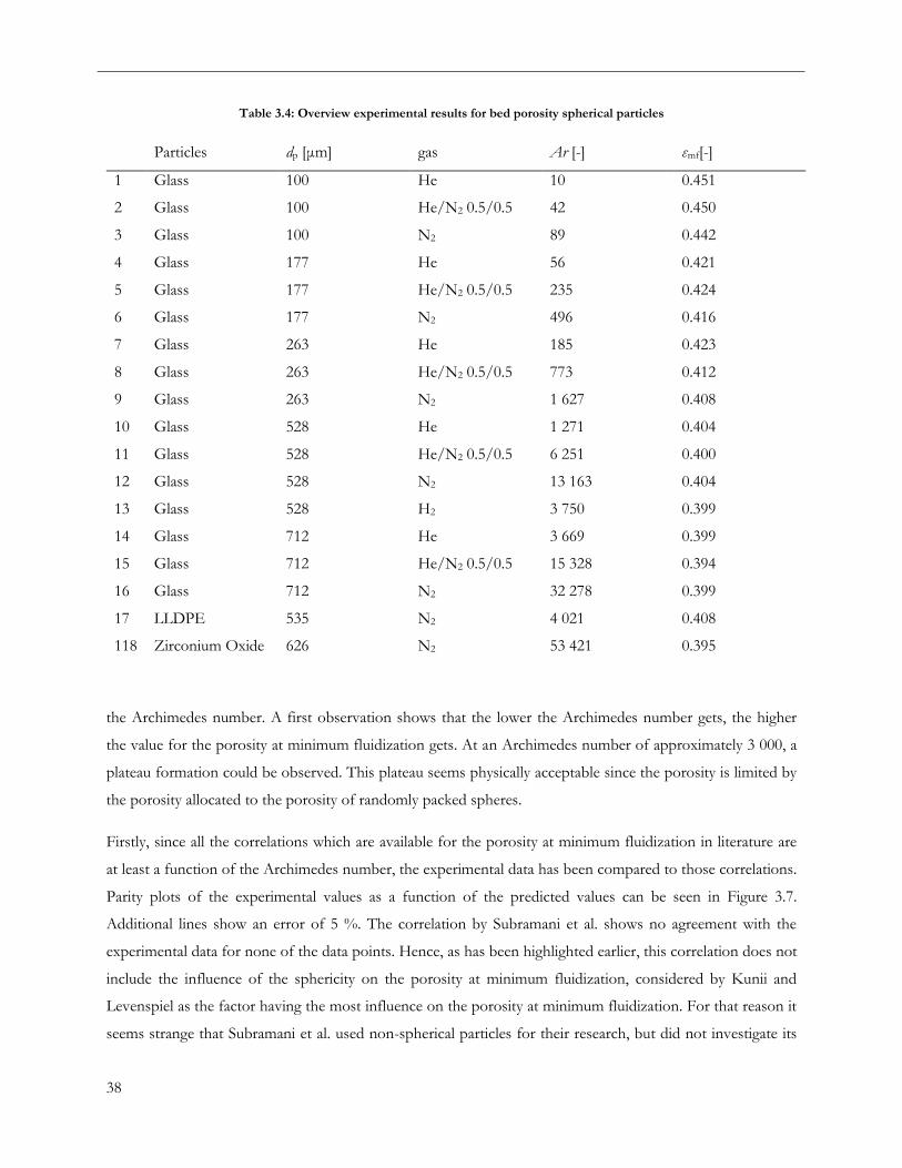
38
Table 3.4: Overview experimental results for bed porosity spherical particles
Particles dp [μm] gas Ar [-] εmf[-]
1 Glass 100 He 10 0.451
2 Glass 100 He/N2 0.5/0.5 42 0.450
3 Glass 100 N2 89 0.442
4 Glass 177 He 56 0.421
5 Glass 177 He/N2 0.5/0.5 235 0.424
6 Glass 177 N2 496 0.416
7 Glass 263 He 185 0.423
8 Glass 263 He/N2 0.5/0.5 773 0.412
9 Glass 263 N2 1 627 0.408
10 Glass 528 He 1 271 0.404
11 Glass 528 He/N2 0.5/0.5 6 251 0.400
12 Glass 528 N2 13 163 0.404
13 Glass 528 H2 3 750 0.399
14 Glass 712 He 3 669 0.399
15 Glass 712 He/N2 0.5/0.5 15 328 0.394
16 Glass 712 N2 32 278 0.399
17 LLDPE 535 N2 4 021 0.408
118 Zirconium Oxide 626 N2 53 421 0.395
the Archimedes number. A first observation shows that the lower the Archimedes number gets, the higher
the value for the porosity at minimum fluidization gets. At an Archimedes number of approximately 3 000, a
plateau formation could be observed. This plateau seems physically acceptable since the porosity is limited by
the porosity allocated to the porosity of randomly packed spheres.
Firstly, since all the correlations which are available for the porosity at minimum fluidization in literature are
at least a function of the Archimedes number, the experimental data has been compared to those correlations.
Parity plots of the experimental values as a function of the predicted values can be seen in Figure 3.7.
Additional lines show an error of 5 %. The correlation by Subramani et al. shows no agreement with the
experimental data for none of the data points. Hence, as has been highlighted earlier, this correlation does not
include the influence of the sphericity on the porosity at minimum fluidization, considered by Kunii and
Levenspiel as the factor having the most influence on the porosity at minimum fluidization. For that reason it
seems strange that Subramani et al. used non-spherical particles for their research, but did not investigate its
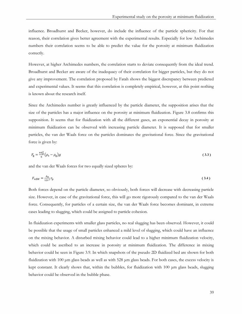
Experimental study on the porosity at minimum fluidization
39
influence. Broadhurst and Becker, however, do include the influence of the particle sphericity. For that
reason, their correlation gives better agreement with the experimental results. Especially for low Archimedes
numbers their correlation seems to be able to predict the value for the porosity at minimum fluidization
correctly.
However, at higher Archimedes numbers, the correlation starts to deviate consequently from the ideal trend.
Broadhurst and Becker are aware of the inadequacy of their correlation for bigger particles, but they do not
give any improvement. The correlation proposed by Fatah shows the biggest discrepancy between predicted
and experimental values. It seems that this correlation is completely empirical, however, at this point nothing
is known about the research itself.
Since the Archimedes number is greatly influenced by the particle diameter, the supposition arises that the
size of the particles has a major influence on the porosity at minimum fluidization. Figure 3.8 confirms this
supposition. It seems that for fluidization with all the different gases, an exponential decay in porosity at
minimum fluidization can be observed with increasing particle diameter. It is supposed that for smaller
particles, the van der Waals force on the particles dominates the gravitational force. Since the gravitational
force is given by:
( 3.3 )
and the van der Waals forces for two equally sized spheres by:
( 3.4 )
Both forces depend on the particle diameter, so obviously, both forces will decrease with decreasing particle
size. However, in case of the gravitational force, this will go more rigorously compared to the van der Waals
force. Consequently, for particles of a certain size, the van der Waals force becomes dominant, in extreme
cases leading to slugging, which could be assigned to particle cohesion.
In fluidization experiments with smaller glass particles, no real slugging has been observed. However, it could
be possible that the usage of small particles enhanced a mild level of slugging, which could have an influence
on the mixing behavior. A disturbed mixing behavior could lead to a higher minimum fluidization velocity,
which could be ascribed to an increase in porosity at minimum fluidization. The difference in mixing
behavior could be seen in Figure 3.9. In which snapshots of the pseudo 2D fluidized bed are shown for both
fluidization with 100 μm glass beads as well as with 528 μm glass beads. For both cases, the excess velocity is
kept constant. It clearly shows that, within the bubbles, for fluidization with 100 μm glass beads, slugging
behavior could be observed in the bubble phase.

40
0.36
0.38
0.40
0.42
0.44
0.46
0.48
0.50
0.52
0.54
0.36 0.38 0.40 0.42 0.44 0.46 0.48 0.50 0.52 0.54
ε mf,
exp
[-]
εmf,pred [-]
Parity plot εmf
+ 5%
- 5%
a
0.36
0.38
0.40
0.42
0.44
0.46
0.48
0.50
0.52
0.54
0.36 0.38 0.40 0.42 0.44 0.46 0.48 0.50 0.52 0.54
ε mf,
exp
[-]
εmf,pred [-]
Parity plot εmf
+ 5%
- 5%
b
0.36
0.38
0.40
0.42
0.44
0.46
0.48
0.50
0.52
0.54
0.36 0.38 0.40 0.42 0.44 0.46 0.48 0.50 0.52 0.54
ε mf,
exp
[-]
εmf,pred [-]
Parity plot εmf
+ 5%
- 5%
c
Figure 3.7: Experimental porosity at minimum fluidization as a function of predicted porosity at minimum fluidization for
present experimental work for a) Subramani et al., b) Broadhurst and Becker and c) Fatah
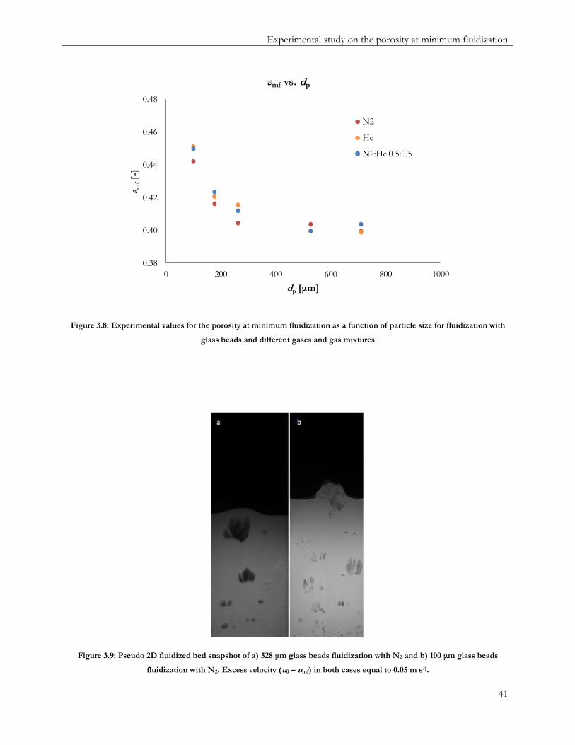
Experimental study on the porosity at minimum fluidization
41
0.38
0.40
0.42
0.44
0.46
0.48
0 200 400 600 800 1000
ε mf[-
]
dp [μm]
εmf vs. dp
N2
He
N2:He 0.5:0.5
Figure 3.8: Experimental values for the porosity at minimum fluidization as a function of particle size for fluidization with
glass beads and different gases and gas mixtures
Figure 3.9: Pseudo 2D fluidized bed snapshot of a) 528 μm glass beads fluidization with N2 and b) 100 μm glass beads
fluidization with N2. Excess velocity (u0 – umf) in both cases equal to 0.05 m s-1.

42
As a first approach to correlate the particle and gas properties to the porosity at minimum fluidization, a
regression analysis on the dimensionless Archimedes number has been carried out. In order to capture the
plateau formation at higher values for the Archimedes number, the following function has been proposed:
( 3.5 )
Fitting parameters for this equation could be found in Table 3.5. For an infinitesimal small value for the
Archimedes number, porosity will go to infinity. Besides, for large values of the Archimedes number the
porosity will go to a. Both Table 3.5 and Figure 3.10 show that a proper fit could be obtained with the
presented parameters. However, to improve the correlation to predict the porosity at minimum fluidization,
gas density has to be taken into account as well. Namely, it could be seen from Figure 3.6 and Figure 3.8 that
the Archimedes number does not perfectly account for the small, but significant role, of the gas density,
especially for small particles. It was noticed by Broadhurst and Becker as well that inserting a dimensionless
density term contributes significantly to reduce the error in the predicted values for the porosity at minimum
fluidization. The form of this correlation would be like this:
( 3.6 )
By using the fitting parameters given in Table 3.5, the porosity at minimum fluidization could be predicted
within an error of 2 % (Figure 3.10). In principle, this would lead to an error of less than 10 % in predicting
the minimum fluidization velocity according to the Ergun or Carman-Kozeny equation.
Table 3.5: Fitting parameters correlations to predict the porosity at minimum fluidization
Variables Ar
Parameter a b R2
Value 0.232 -0.037
Standard error 0.003 0.005
R-square 0.72
Variables Ar ρp/ρg
Parameter a b c R2
Value 0.382 -0.217 -0.126
Standard error 0.007 0.011 0.007
R-square 0.88
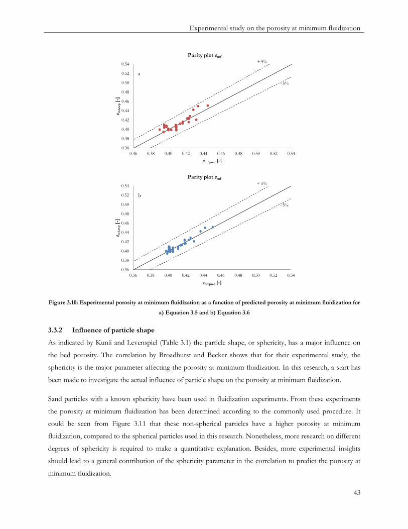
Experimental study on the porosity at minimum fluidization
43
0.36
0.38
0.40
0.42
0.44
0.46
0.48
0.50
0.52
0.54
0.36 0.38 0.40 0.42 0.44 0.46 0.48 0.50 0.52 0.54
ε mf,
exp
[-]
εmf,pred [-]
Parity plot εmf
+ 5%
- 5%
a
0.36
0.38
0.40
0.42
0.44
0.46
0.48
0.50
0.52
0.54
0.36 0.38 0.40 0.42 0.44 0.46 0.48 0.50 0.52 0.54
ε mf,
exp
[-]
εmf,pred [-]
Parity plot εmf
+ 5%
- 5%
b
Figure 3.10: Experimental porosity at minimum fluidization as a function of predicted porosity at minimum fluidization for
a) Equation 3.5 and b) Equation 3.6
3.3.2 Influence of particle shape
As indicated by Kunii and Levenspiel (Table 3.1) the particle shape, or sphericity, has a major influence on
the bed porosity. The correlation by Broadhurst and Becker shows that for their experimental study, the
sphericity is the major parameter affecting the porosity at minimum fluidization. In this research, a start has
been made to investigate the actual influence of particle shape on the porosity at minimum fluidization.
Sand particles with a known sphericity have been used in fluidization experiments. From these experiments
the porosity at minimum fluidization has been determined according to the commonly used procedure. It
could be seen from Figure 3.11 that these non-spherical particles have a higher porosity at minimum
fluidization, compared to the spherical particles used in this research. Nonetheless, more research on different
degrees of sphericity is required to make a quantitative explanation. Besides, more experimental insights
should lead to a general contribution of the sphericity parameter in the correlation to predict the porosity at
minimum fluidization.
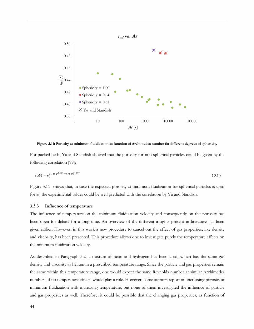
44
0.38
0.40
0.42
0.44
0.46
0.48
0.50
1 10 100 1000 10000 100000
ε mf [-
]
Ar [-]
εmf vs. Ar
Sphericity = 1.00
Sphericity = 0.64
Sphericity = 0.61
× Yu and Standish
Figure 3.11: Porosity at minimum fluidization as function of Archimedes number for different degrees of sphericity
For packed beds, Yu and Standish showed that the porosity for non-spherical particles could be given by the
following correlation [99]:
( 3.7 )
Figure 3.11 shows that, in case the expected porosity at minimum fluidization for spherical particles is used
for ε0, the experimental values could be well predicted with the correlation by Yu and Standish.
3.3.3 Influence of temperature
The influence of temperature on the minimum fluidization velocity and consequently on the porosity has
been open for debate for a long time. An overview of the different insights present in literature has been
given earlier. However, in this work a new procedure to cancel out the effect of gas properties, like density
and viscosity, has been presented. This procedure allows one to investigate purely the temperature effects on
the minimum fluidization velocity.
As described in Paragraph 3.2, a mixture of neon and hydrogen has been used, which has the same gas
density and viscosity as helium in a prescribed temperature range. Since the particle and gas properties remain
the same within this temperature range, one would expect the same Reynolds number at similar Archimedes
numbers, if no temperature effects would play a role. However, some authors report on increasing porosity at
minimum fluidization with increasing temperature, but none of them investigated the influence of particle
and gas properties as well. Therefore, it could be possible that the changing gas properties, as function of
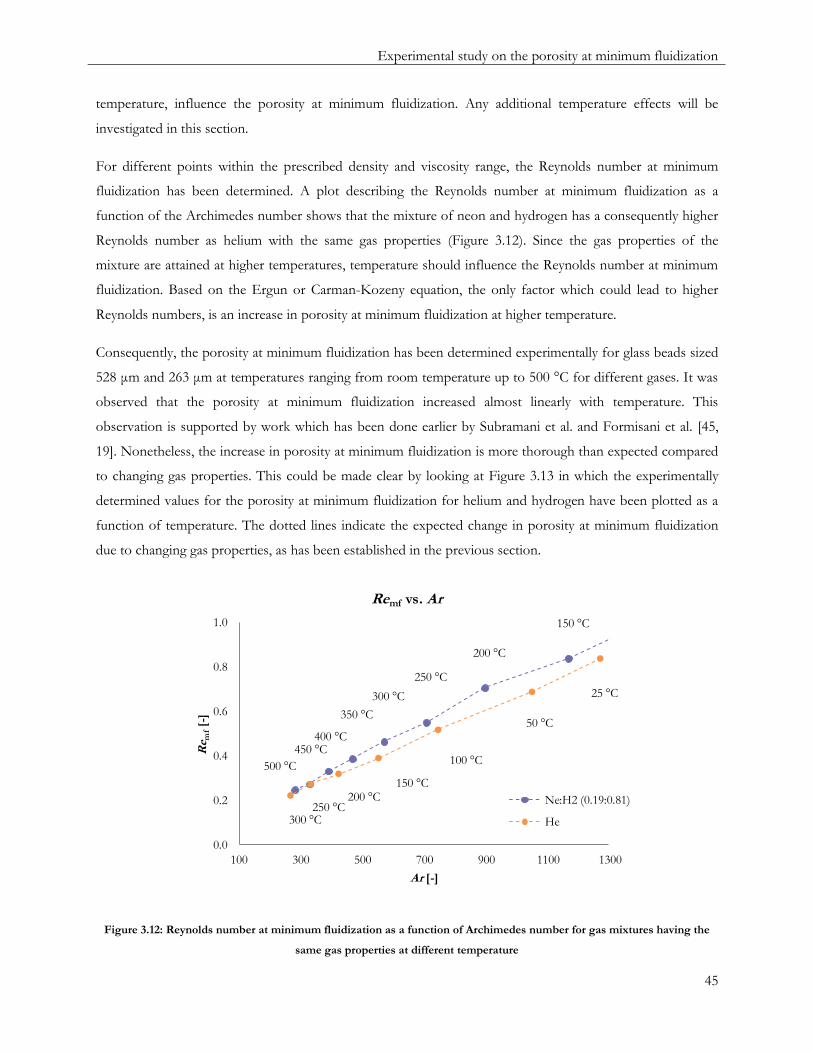
Experimental study on the porosity at minimum fluidization
45
temperature, influence the porosity at minimum fluidization. Any additional temperature effects will be
investigated in this section.
For different points within the prescribed density and viscosity range, the Reynolds number at minimum
fluidization has been determined. A plot describing the Reynolds number at minimum fluidization as a
function of the Archimedes number shows that the mixture of neon and hydrogen has a consequently higher
Reynolds number as helium with the same gas properties (Figure 3.12). Since the gas properties of the
mixture are attained at higher temperatures, temperature should influence the Reynolds number at minimum
fluidization. Based on the Ergun or Carman-Kozeny equation, the only factor which could lead to higher
Reynolds numbers, is an increase in porosity at minimum fluidization at higher temperature.
Consequently, the porosity at minimum fluidization has been determined experimentally for glass beads sized
528 μm and 263 μm at temperatures ranging from room temperature up to 500 °C for different gases. It was
observed that the porosity at minimum fluidization increased almost linearly with temperature. This
observation is supported by work which has been done earlier by Subramani et al. and Formisani et al. [45,
19]. Nonetheless, the increase in porosity at minimum fluidization is more thorough than expected compared
to changing gas properties. This could be made clear by looking at Figure 3.13 in which the experimentally
determined values for the porosity at minimum fluidization for helium and hydrogen have been plotted as a
function of temperature. The dotted lines indicate the expected change in porosity at minimum fluidization
due to changing gas properties, as has been established in the previous section.
150 °C
200 °C
250 °C
300 °C
350 °C
400 °C450 °C
500 °C
25 °C
50 °C
100 °C
150 °C200 °C
250 °C300 °C
0.0
0.2
0.4
0.6
0.8
1.0
100 300 500 700 900 1100 1300
Re m
f[-
]
Ar [-]
Remf vs. Ar
Ne:H2 (0.19:0.81)
He
Figure 3.12: Reynolds number at minimum fluidization as a function of Archimedes number for gas mixtures having the
same gas properties at different temperature
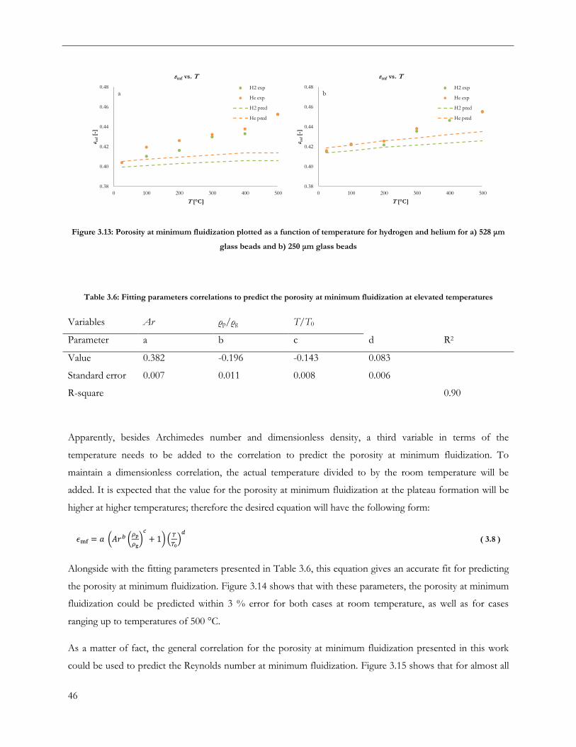
46
0.38
0.40
0.42
0.44
0.46
0.48
0 100 200 300 400 500
ε mf[-
]
T [°C]
εmf vs. T
H2 exp
He exp
H2 pred
He pred
a
0.38
0.40
0.42
0.44
0.46
0.48
0 100 200 300 400 500
ε mf[-
]
T [°C]
εmf vs. T
H2 exp
He exp
H2 pred
He pred
b
Figure 3.13: Porosity at minimum fluidization plotted as a function of temperature for hydrogen and helium for a) 528 μm
glass beads and b) 250 μm glass beads
Table 3.6: Fitting parameters correlations to predict the porosity at minimum fluidization at elevated temperatures
Variables Ar ρp/ρg T/T0
Parameter a b c d R2
Value 0.382 -0.196 -0.143 0.083
Standard error 0.007 0.011 0.008 0.006
R-square 0.90
Apparently, besides Archimedes number and dimensionless density, a third variable in terms of the
temperature needs to be added to the correlation to predict the porosity at minimum fluidization. To
maintain a dimensionless correlation, the actual temperature divided to by the room temperature will be
added. It is expected that the value for the porosity at minimum fluidization at the plateau formation will be
higher at higher temperatures; therefore the desired equation will have the following form:
( 3.8 )
Alongside with the fitting parameters presented in Table 3.6, this equation gives an accurate fit for predicting
the porosity at minimum fluidization. Figure 3.14 shows that with these parameters, the porosity at minimum
fluidization could be predicted within 3 % error for both cases at room temperature, as well as for cases
ranging up to temperatures of 500 °C.
As a matter of fact, the general correlation for the porosity at minimum fluidization presented in this work
could be used to predict the Reynolds number at minimum fluidization. Figure 3.15 shows that for almost all
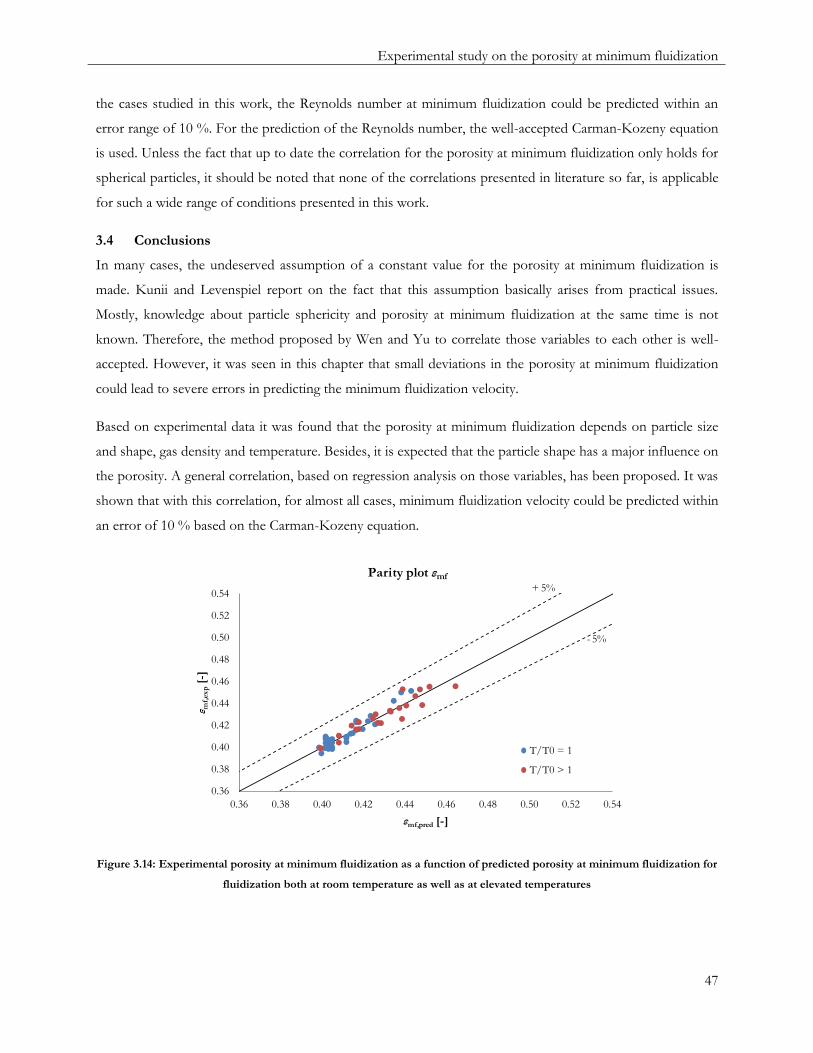
Experimental study on the porosity at minimum fluidization
47
the cases studied in this work, the Reynolds number at minimum fluidization could be predicted within an
error range of 10 %. For the prediction of the Reynolds number, the well-accepted Carman-Kozeny equation
is used. Unless the fact that up to date the correlation for the porosity at minimum fluidization only holds for
spherical particles, it should be noted that none of the correlations presented in literature so far, is applicable
for such a wide range of conditions presented in this work.
3.4 Conclusions
In many cases, the undeserved assumption of a constant value for the porosity at minimum fluidization is
made. Kunii and Levenspiel report on the fact that this assumption basically arises from practical issues.
Mostly, knowledge about particle sphericity and porosity at minimum fluidization at the same time is not
known. Therefore, the method proposed by Wen and Yu to correlate those variables to each other is well-
accepted. However, it was seen in this chapter that small deviations in the porosity at minimum fluidization
could lead to severe errors in predicting the minimum fluidization velocity.
Based on experimental data it was found that the porosity at minimum fluidization depends on particle size
and shape, gas density and temperature. Besides, it is expected that the particle shape has a major influence on
the porosity. A general correlation, based on regression analysis on those variables, has been proposed. It was
shown that with this correlation, for almost all cases, minimum fluidization velocity could be predicted within
an error of 10 % based on the Carman-Kozeny equation.
0.36
0.38
0.40
0.42
0.44
0.46
0.48
0.50
0.52
0.54
0.36 0.38 0.40 0.42 0.44 0.46 0.48 0.50 0.52 0.54
ε mf,
exp
[-]
εmf,pred [-]
Parity plot εmf
T/T0 = 1
T/T0 > 1
+ 5%
- 5%
Figure 3.14: Experimental porosity at minimum fluidization as a function of predicted porosity at minimum fluidization for
fluidization both at room temperature as well as at elevated temperatures
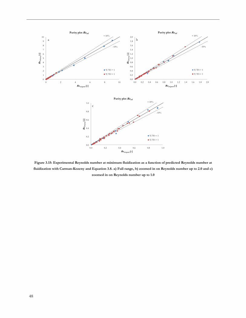
48
0
1
2
3
4
5
6
7
8
9
10
0 2 4 6 8 10
Re
mf,
exp
[-]
Remf,pred [-]
Parity plot Remf
T/T0 = 1
T/T0 > 1
+ 10%
- 10%
a
0.0
0.2
0.4
0.6
0.8
1.0
1.2
1.4
1.6
1.8
2.0
0.0 0.2 0.4 0.6 0.8 1.0 1.2 1.4 1.6 1.8 2.0
Re
mf,
exp
[-]
Remf,pred [-]
Parity plot Remf
T/T0 = 1
T/T0 > 1
+ 10%
- 10%
b
0.0
0.2
0.4
0.6
0.8
1.0
0.0 0.2 0.4 0.6 0.8 1.0
Re
mf,
exp
[-]
Remf,pred [-]
Parity plot Remf
T/T0 = 1
T/T0 > 1
+ 10%
- 10%
c
Figure 3.15: Experimental Reynolds number at minimum fluidization as a function of predicted Reynolds number at
fluidization with Carman-Kozeny and Equation 3.8. a) Full range, b) zoomed in on Reynolds number up to 2.0 and c)
zoomed in on Reynolds number up to 1.0

Hydrodynamics of bubbling fluidized beds
49
4 Hydrodynamics of bubbling fluidized beds
In this chapter, the hydrodynamics of a bubbling fluidized bed have been studied. A pseudo 2D column packed with both glass
particles sized 177 μm as well as 528 μm has been analyzed with the non-invasive digital image analysis (DIA) technique.
Based on a threshold value, this technique discriminated between bubble and emulsion phase, which makes it possible to
determine bubble hold-up, bubble size, bubble velocity and visual bubble flow rate. The experimental findings have been compared
to correlations which are available in open literature. It was found that the larger glass beads correspond reasonably well with
literature correlations. Moreover, the difference in hydrodynamics between small and larger particles could be related to the
difference in porosity at minimum fluidization between those particles.
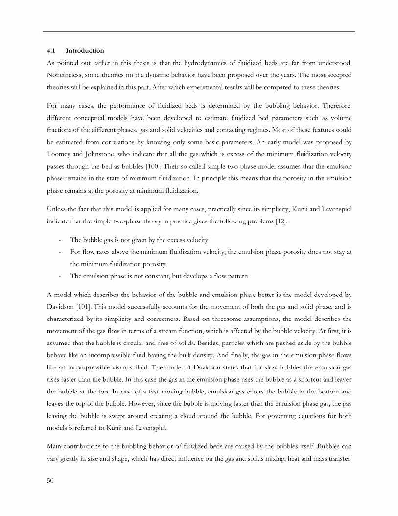
50
4.1 Introduction
As pointed out earlier in this thesis is that the hydrodynamics of fluidized beds are far from understood.
Nonetheless, some theories on the dynamic behavior have been proposed over the years. The most accepted
theories will be explained in this part. After which experimental results will be compared to these theories.
For many cases, the performance of fluidized beds is determined by the bubbling behavior. Therefore,
different conceptual models have been developed to estimate fluidized bed parameters such as volume
fractions of the different phases, gas and solid velocities and contacting regimes. Most of these features could
be estimated from correlations by knowing only some basic parameters. An early model was proposed by
Toomey and Johnstone, who indicate that all the gas which is excess of the minimum fluidization velocity
passes through the bed as bubbles [100]. Their so-called simple two-phase model assumes that the emulsion
phase remains in the state of minimum fluidization. In principle this means that the porosity in the emulsion
phase remains at the porosity at minimum fluidization.
Unless the fact that this model is applied for many cases, practically since its simplicity, Kunii and Levenspiel
indicate that the simple two-phase theory in practice gives the following problems [12]:
- The bubble gas is not given by the excess velocity
- For flow rates above the minimum fluidization velocity, the emulsion phase porosity does not stay at
the minimum fluidization porosity
- The emulsion phase is not constant, but develops a flow pattern
A model which describes the behavior of the bubble and emulsion phase better is the model developed by
Davidson [101]. This model successfully accounts for the movement of both the gas and solid phase, and is
characterized by its simplicity and correctness. Based on threesome assumptions, the model describes the
movement of the gas flow in terms of a stream function, which is affected by the bubble velocity. At first, it is
assumed that the bubble is circular and free of solids. Besides, particles which are pushed aside by the bubble
behave like an incompressible fluid having the bulk density. And finally, the gas in the emulsion phase flows
like an incompressible viscous fluid. The model of Davidson states that for slow bubbles the emulsion gas
rises faster than the bubble. In this case the gas in the emulsion phase uses the bubble as a shortcut and leaves
the bubble at the top. In case of a fast moving bubble, emulsion gas enters the bubble in the bottom and
leaves the top of the bubble. However, since the bubble is moving faster than the emulsion phase gas, the gas
leaving the bubble is swept around creating a cloud around the bubble. For governing equations for both
models is referred to Kunii and Levenspiel.
Main contributions to the bubbling behavior of fluidized beds are caused by the bubbles itself. Bubbles can
vary greatly in size and shape, which has direct influence on the gas and solids mixing, heat and mass transfer,
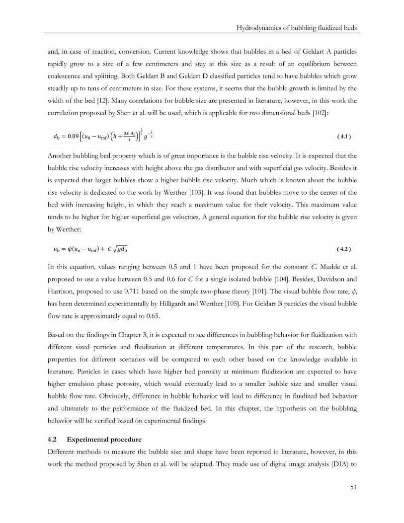
Hydrodynamics of bubbling fluidized beds
51
and, in case of reaction, conversion. Current knowledge shows that bubbles in a bed of Geldart A particles
rapidly grow to a size of a few centimeters and stay at this size as a result of an equilibrium between
coalescence and splitting. Both Geldart B and Geldart D classified particles tend to have bubbles which grow
steadily up to tens of centimeters in size. For these systems, it seems that the bubble growth is limited by the
width of the bed [12]. Many correlations for bubble size are presented in literature, however, in this work the
correlation proposed by Shen et al. will be used, which is applicable for two dimensional beds [102]:
( 4.1 )
Another bubbling bed property which is of great importance is the bubble rise velocity. It is expected that the
bubble rise velocity increases with height above the gas distributor and with superficial gas velocity. Besides it
is expected that larger bubbles show a higher bubble rise velocity. Much which is known about the bubble
rise velocity is dedicated to the work by Werther [103]. It was found that bubbles move to the center of the
bed with increasing height, in which they reach a maximum value for their velocity. This maximum value
tends to be higher for higher superficial gas velocities. A general equation for the bubble rise velocity is given
by Werther:
( 4.2 )
In this equation, values ranging between 0.5 and 1 have been proposed for the constant C. Mudde et al.
proposed to use a value between 0.5 and 0.6 for C for a single isolated bubble [104]. Besides, Davidson and
Harrison, proposed to use 0.711 based on the simple two-phase theory [101]. The visual bubble flow rate, ψ,
has been determined experimentally by Hilligardt and Werther [105]. For Geldart B particles the visual bubble
flow rate is approximately equal to 0.65.
Based on the findings in Chapter 3, it is expected to see differences in bubbling behavior for fluidization with
different sized particles and fluidization at different temperatures. In this part of the research, bubble
properties for different scenarios will be compared to each other based on the knowledge available in
literature. Particles in cases which have higher bed porosity at minimum fluidization are expected to have
higher emulsion phase porosity, which would eventually lead to a smaller bubble size and smaller visual
bubble flow rate. Obviously, difference in bubble behavior will lead to difference in fluidized bed behavior
and ultimately to the performance of the fluidized bed. In this chapter, the hypothesis on the bubbling
behavior will be verified based on experimental findings.
4.2 Experimental procedure
Different methods to measure the bubble size and shape have been reported in literature, however, in this
work the method proposed by Shen et al. will be adapted. They made use of digital image analysis (DIA) to
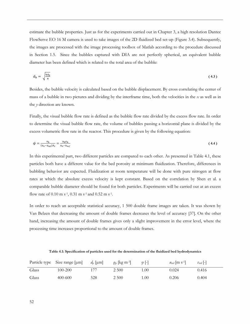
52
estimate the bubble properties. Just as for the experiments carried out in Chapter 3, a high resolution Dantec
FlowServe EO 16 M camera is used to take images of the 2D fluidized bed set-up (Figure 3.4). Subsequently,
the images are processed with the image processing toolbox of Matlab according to the procedure discussed
in Section 1.5. Since the bubbles captured with DIA are not perfectly spherical, an equivalent bubble
diameter has been defined which is related to the total area of the bubble:
( 4.3 )
Besides, the bubble velocity is calculated based on the bubble displacement. By cross correlating the center of
mass of a bubble in two pictures and dividing by the interframe time, both the velocities in the x as well as in
the y direction are known.
Finally, the visual bubble flow rate is defined as the bubble flow rate divided by the excess flow rate. In order
to determine the visual bubble flow rate, the volume of bubbles passing a horizontal plane is divided by the
excess volumetric flow rate in the reactor. This procedure is given by the following equation:
( 4.4 )
In this experimental part, two different particles are compared to each other. As presented in Table 4.1, these
particles both have a different value for the bed porosity at minimum fluidization. Therefore, differences in
bubbling behavior are expected. Fluidization at room temperature will be done with pure nitrogen at flow
rates at which the absolute excess velocity is kept constant. Based on the correlation by Shen et al. a
comparable bubble diameter should be found for both particles. Experiments will be carried out at an excess
flow rate of 0.10 m s-1, 0.31 m s-1 and 0.52 m s-1.
In order to reach an acceptable statistical accuracy, 1 500 double frame images are taken. It was shown by
Van Belzen that decreasing the amount of double frames decreases the level of accuracy [37]. On the other
hand, increasing the amount of double frames gives only a slight improvement in the error level, where the
processing time increases proportional to the amount of double frames.
Table 4.1: Specification of particles used for the determination of the fluidized bed hydrodynamics
Particle type Size range [μm] dp [μm] ρp [kg m-3] φ [-] umf [m s-1] εmf [-]
Glass 100-200 177 2 500 1.00 0.024 0.416
Glass 400-600 528 2 500 1.00 0.206 0.404

Hydrodynamics of bubbling fluidized beds
53
4.3 Results and discussion
Bubble properties of both beds of particles of 177 μm as well as 528 μm have been compared to each other
and literature results. Figures which show the equivalent bubble diameter as a function of height in the bed
are presented in Figure 4.1. For both cases, 2.0 kg of particles have been loaded into the bed. It should be
noted that for the 177 μm particles the aspect ratio of the packed bed was higher than for the 528 μm glass
beads. However, as investigated by Laverman et al., the aspect ratio of the initial packed bed, has no influence
on the bubble size [29]. The equivalent bubble properties have been compared to the correlation proposed by
Shen et al. (Equation 4.1). For both particles, the absolute excess velocity has been kept constant, so in
theory, for the same excess velocity, the same bubble size as a function of bed height is expected for both
particles.
It can be seen that for the 528 μm glass beads, the determined equivalent bubble diameter matches perfectly
with the Shen et al. correlation for the excess flow rates of 0.10 m s-1 and 0.32 m s-1. For an excess flow rate
of 0.52 m s-1 the experimental results are over predicted by the correlation. This deviation in correlation and
experimental results could be explained by the greater bed dimensions used by Shen et al. Namely, at higher
excess flow rates bigger bubbles are expected. However, in the present work, the bubble growth is limited by
the bed dimensions.
For fluidization with 177 μm glass beads a severe over predicting of the experimental results is observed
compared to the correlation by Shen. Since the smaller particles exhibit a significantly higher porosity at
minimum fluidization, higher emulsion phase porosity is expected too. This presumption is confirmed by
Figure 4.2 which shows both the average bed porosity as well as the emulsion phase porosity as a function of
the excess flow rate. It could be observed that smaller particles have a higher emulsion phase porosity, which
in its turn allows more gas in the emulsion phase, resulting in smaller bubbles. Figure 4.3 compares the
number of bubbles for both fluidization with 177 μm as well as 528 μm glass beads with a constant excess
velocity of 0.32 m s-1. If one takes a look at the total number of bubbles as a function of bubble diameter, it
could be seen that indeed a remarkable amount of smaller bubbles is present when smaller particles are used
for fluidization.
An additional explanation for the smaller bubbles arises from the fact that the DIA script has difficulties in
detecting bubbles for the totally different bubbling behavior for smaller particles. This behavior, which is
ascribed to increasing van der Waals force for smaller particles, leads to a totally different behavior of the
particle rain in the bubbles. Due to the increased van der Waals force, cohesion of particles is enhanced,
which leads to slugging particle rain. This divides the bubble into different parts, which means that DIA
detects more smaller bubbles, instead of one bigger. This behavior is visualized in Figure 4.4.
54
0.00
0.02
0.04
0.06
0.08
0.10
0.12
0.14
0.16
0.00 0.05 0.10 0.15 0.20 0.25 0.30 0.35 0.40
db
[m]
h [m]
db vs. h
u0-umf = 0.10 m/s
u0-umf = 0.31 m/s
u0-umf = 0.52 m/s
a
- - Shen et al.
0.00
0.02
0.04
0.06
0.08
0.10
0.12
0.14
0.16
0.00 0.05 0.10 0.15 0.20 0.25 0.30 0.35 0.40
db
[m]
h [m]
db vs. h
u0-umf = 0.10 m/s
u0-umf = 0.31 m/s
u0-umf = 0.52 m/s
b
- - Shen et al.
Figure 4.1: Equivalent bubble diameter as a function of bed height for fluidization with nitrogen, excess flow rates of 0.10
m s-1, 0.32 m s-1 and 0.52 m s-1. a) 528 μm glass beads and b) 177 μm glass beads
0.40
0.45
0.50
0.55
0.60
0.65
0.70
0.0 0.1 0.2 0.3 0.4 0.5 0.6
ε[-
]
u0-umf [m s-1]
ε vs. u0-umf
• average bed porosity
▪ emulsion phase porosity
177 μm glass beads528 μm glass beads
Figure 4.2: Average bed porosity and emulsion phase porosity as a function of excess flow rate for fluidization with
nitrogen and 177 μm and 528 μm glass beads
0
1000
2000
3000
4000
5000
6000
0.00 0.02 0.04 0.06 0.08 0.10 0.12 0.14 0.16
Nb
[-]
db [m]
Nb vs. db
177 μm glass beads528 μm glass beads
Figure 4.3: Total number of bubbles as a function of equivalent bubble diameter for fluidization with nitrogen and 177 μm
and 528 μm glass beads (u0-umf = 0.32 m s-1). Amount of dubble frame images is equal to 1500.
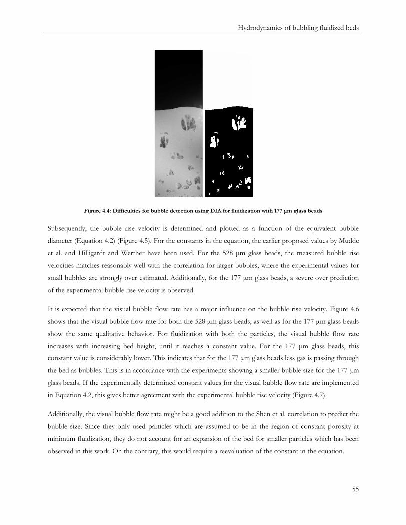
Hydrodynamics of bubbling fluidized beds
55
Figure 4.4: Difficulties for bubble detection using DIA for fluidization with 177 μm glass beads
Subsequently, the bubble rise velocity is determined and plotted as a function of the equivalent bubble
diameter (Equation 4.2) (Figure 4.5). For the constants in the equation, the earlier proposed values by Mudde
et al. and Hilligardt and Werther have been used. For the 528 μm glass beads, the measured bubble rise
velocities matches reasonably well with the correlation for larger bubbles, where the experimental values for
small bubbles are strongly over estimated. Additionally, for the 177 μm glass beads, a severe over prediction
of the experimental bubble rise velocity is observed.
It is expected that the visual bubble flow rate has a major influence on the bubble rise velocity. Figure 4.6
shows that the visual bubble flow rate for both the 528 μm glass beads, as well as for the 177 μm glass beads
show the same qualitative behavior. For fluidization with both the particles, the visual bubble flow rate
increases with increasing bed height, until it reaches a constant value. For the 177 μm glass beads, this
constant value is considerably lower. This indicates that for the 177 μm glass beads less gas is passing through
the bed as bubbles. This is in accordance with the experiments showing a smaller bubble size for the 177 μm
glass beads. If the experimentally determined constant values for the visual bubble flow rate are implemented
in Equation 4.2, this gives better agreement with the experimental bubble rise velocity (Figure 4.7).
Additionally, the visual bubble flow rate might be a good addition to the Shen et al. correlation to predict the
bubble size. Since they only used particles which are assumed to be in the region of constant porosity at
minimum fluidization, they do not account for an expansion of the bed for smaller particles which has been
observed in this work. On the contrary, this would require a reevaluation of the constant in the equation.

56
0.0
0.2
0.4
0.6
0.8
1.0
1.2
0.00 0.02 0.04 0.06 0.08 0.10
ub
[m s
-1]
db [m]
ub vs. db
u0-umf = 0.10 m/s
u0-umf = 0.31 m/s
u0-umf = 0.52 m/s
a
0.0
0.2
0.4
0.6
0.8
1.0
1.2
0.00 0.02 0.04 0.06 0.08 0.10
ub
[m s
-1]
db [m]
ub vs. db
u0-umf = 0.10 m/s
u0-umf = 0.31 m/s
u0-umf = 0.52 m/s
b
Figure 4.5: Bubble rise velocity as a function of equivalent bubble diameter for fluidization with nitrogen and a) 528 μm
glass beads and b) 177 μm glass beads. Constants by Mudde et al. and Hilligardt and Werther
0.0
0.1
0.2
0.3
0.4
0.5
0.6
0.7
0.0 0.2 0.4 0.6 0.8 1.0
ψ[-
]
h/h0 [-]
ψ vs. h/h0
u0-umf = 0.10 m/s
u0-umf = 0.31 m/s
u0-umf = 0.52 m/s
a
0.0
0.1
0.2
0.3
0.4
0.5
0.6
0.7
0.0 0.2 0.4 0.6 0.8 1.0
ψ[-
]
h/h0 [-]
ψ vs. h/h0
u0-umf = 0.10 m/s
u0-umf = 0.31 m/s
u0-umf = 0.52 m/s
b
Figure 4.6: Visual bubble flow rate as function of dimensionless bed height for fluidization with nitrogen and a) 528 μm
glass beads and b) 177 μm glass beads.
0.0
0.2
0.4
0.6
0.8
1.0
1.2
0.00 0.02 0.04 0.06 0.08 0.10
ub
[m s
-1]
db [m]
ub vs. db
u0-umf = 0.10 m/s
u0-umf = 0.31 m/s
u0-umf = 0.52 m/s
a
0.0
0.2
0.4
0.6
0.8
1.0
1.2
0.00 0.02 0.04 0.06 0.08 0.10
ub
[m s
-1]
db [m]
ub vs. db
u0-umf = 0.10 m/s
u0-umf = 0.31 m/s
u0-umf = 0.52 m/s
b
Figure 4.7: Bubble rise velocity as a function of equivalent bubble diameter for fluidization with nitrogen and a) 528 μm
glass beads and b) 177 μm glass beads. Constants determined experimentally.
Hydrodynamics of bubbling fluidized beds
57
4.4 Conclusions
The bubbling behavior of fluidized beds seems to be the major parameter influencing its performance. Since
the occurrence of bubbles is directly related to for instance mixing behavior, heat and mass transfer and
chemical reaction, it is important to understand the bubbling behavior. In the current part of this work it was
shown that bubble properties can be directly related to the change in porosity at minimum fluidization
conditions, which has been discussed in Chapter 3. Due to the change in emulsion phase porosity, bubble
properties like equivalent bubble size and bubble rise velocity tend to change.
Most important parameter which could correct for the difference in bubbling behavior is the visual bubble
flow rate. It defines the fraction of gas passing the column as bubbles. In cases of smaller particles, the value
of this parameter would be smaller compared to bigger particles, since smaller particles have a less dense
packing of the bed. It is expected that correcting for this visual bubble flow rate would improve the
correlation by Shen et al. to predict bubble size.

58
Forces in fluidized beds
59
5 Forces in fluidized beds
Fluidization behavior of particle beds is observed when the drag force exerted by the gas equals the particle weight force. However,
it seems that interparticle forces should also be accounted for studying the dynamic behavior of fluidized beds. In the past, different
research groups have investigated the influence of interparticle forces, but the nature of these phenomena is still uncertain. In this
chapter, an overview of the different interparticle forces is given, which might influence the behavior of particles in fluidized beds.
Based on current insights, it seems most likely that the van der Waals force has a major influence on particle packing for
especially small particles. Due to the cohesive nature, small particles are assumed to act as aggregates, which thwart fluidization.
This effect is reinforced at higher temperature, where the van der Waals force is likely to increase with temperature.
60
5.1 Introduction
Different researchers have suggested that changing interparticle forces might be the cause for the different
fluidization behavior at high temperatures [18, 21, 106]. However, none of them has attributed the change to
a specific force or investigated whether this change could also be observed for different particle or gas
properties at room temperature. In this chapter, an overview will be given of which interparticle forces might
be present in fluidization processes. Besides, a theory, based on changing interparticle forces will be
developed in order to explain the fluidization behavior seen in this work so far.
Up to date, most of the predicting of fluidization behavior has been based on the work of Geldart [107]. In
the Geldart classification, four different kinds of behaviors can be distinguished, which are mainly based on
both density differences between gas and particles and the particle size. However, it seems that the Geldart
classification is only applicable in general cases, since its boundaries of groups may change when the
hydrodynamic and interparticle forces change. In principle this would mean that some particles which in
theory are classified as Geldart A could act as either Geldart B or Geldart C as a result of variations between
hydrodynamic and interparticle forces. To cope up with this problem, a modification to the Geldart
classification, making use of interface areas AB and AC, have been proposed [106].
In recent years, different researchers investigated the effect of temperature on interparticle forces in
fluidization. However, to date, there is no agreement on how the interparticle forces might affect high
temperature fluidization. In order to better understand the interparticle forces, first, the possible interparticle
forces will be analyzed and discussed briefly.
It was reported by Visser that the dominant interaction force between particles in a powder, as well as in a
fluidized bed is the van der Waals force [108]. However, its magnitude becomes negligible compared to the
gravitational force as particles get bigger. As some intermolecular forces only occur with some particle type or
material, van der Waals forces always exist. The nature of the van der Waals force is the charge interactions
between the atoms and molecules. These interactions can be dipole-dipole, dipole-induced dipole and
dispersion forces. If spherical particles are considered, which contain many atoms or molecules, the van der
Waals force can be determined according to the following equation [109]:
( 5.1 )
The Hamaker constant (AH) is considered to be a material constant. Typical values are found in the order of
10-20 J to 10-19 J. For many engineering applications, the separation distance of the particles is negligible
compared to the particle size. In that case, Equation 5.1 could be simplified to:
( 5.2 )
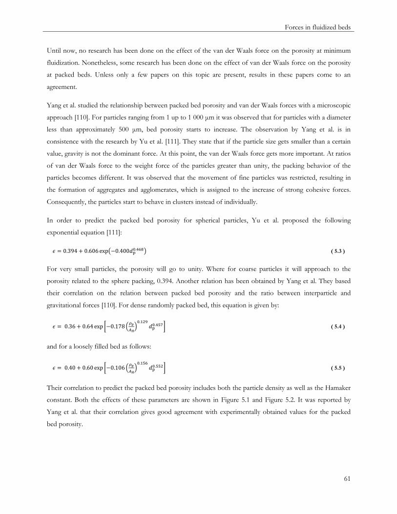
Forces in fluidized beds
61
Until now, no research has been done on the effect of the van der Waals force on the porosity at minimum
fluidization. Nonetheless, some research has been done on the effect of van der Waals force on the porosity
at packed beds. Unless only a few papers on this topic are present, results in these papers come to an
agreement.
Yang et al. studied the relationship between packed bed porosity and van der Waals forces with a microscopic
approach [110]. For particles ranging from 1 up to 1 000 μm it was observed that for particles with a diameter
less than approximately 500 μm, bed porosity starts to increase. The observation by Yang et al. is in
consistence with the research by Yu et al. [111]. They state that if the particle size gets smaller than a certain
value, gravity is not the dominant force. At this point, the van der Waals force gets more important. At ratios
of van der Waals force to the weight force of the particles greater than unity, the packing behavior of the
particles becomes different. It was observed that the movement of fine particles was restricted, resulting in
the formation of aggregates and agglomerates, which is assigned to the increase of strong cohesive forces.
Consequently, the particles start to behave in clusters instead of individually.
In order to predict the packed bed porosity for spherical particles, Yu et al. proposed the following
exponential equation [111]:
( 5.3 )
For very small particles, the porosity will go to unity. Where for coarse particles it will approach to the
porosity related to the sphere packing, 0.394. Another relation has been obtained by Yang et al. They based
their correlation on the relation between packed bed porosity and the ratio between interparticle and
gravitational forces [110]. For dense randomly packed bed, this equation is given by:
( 5.4 )
and for a loosely filled bed as follows:
( 5.5 )
Their correlation to predict the packed bed porosity includes both the particle density as well as the Hamaker
constant. Both the effects of these parameters are shown in Figure 5.1 and Figure 5.2. It was reported by
Yang et al. that their correlation gives good agreement with experimentally obtained values for the packed
bed porosity.
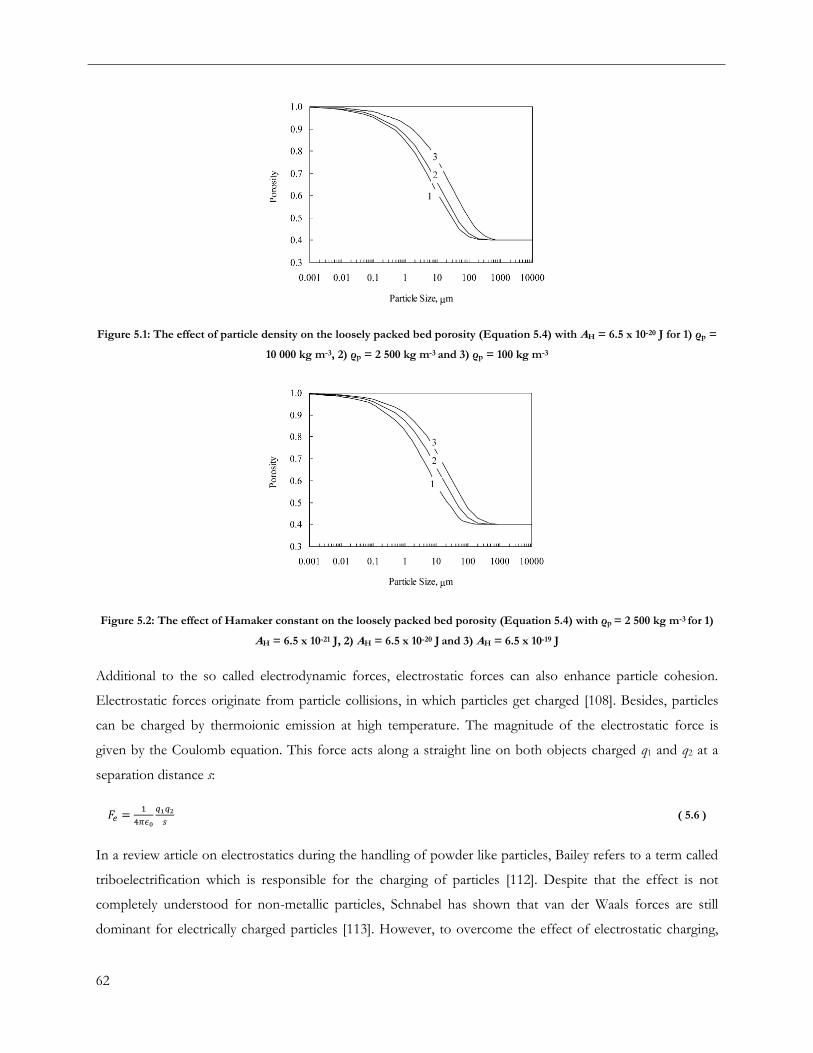
62
Figure 5.1: The effect of particle density on the loosely packed bed porosity (Equation 5.4) with AH = 6.5 x 10⁻²⁰ J for 1) ρp =
10 000 kg m-3, 2) ρp = 2 500 kg m-3 and 3) ρp = 100 kg m-3
Figure 5.2: The effect of Hamaker constant on the loosely packed bed porosity (Equation 5.4) with ρp = 2 500 kg m-3 for 1)
AH = 6.5 x 10⁻²¹ J, 2) AH = 6.5 x 10⁻²⁰ J and 3) AH = 6.5 x 10⁻¹⁹ J
Additional to the so called electrodynamic forces, electrostatic forces can also enhance particle cohesion.
Electrostatic forces originate from particle collisions, in which particles get charged [108]. Besides, particles
can be charged by thermoionic emission at high temperature. The magnitude of the electrostatic force is
given by the Coulomb equation. This force acts along a straight line on both objects charged q1 and q2 at a
separation distance s:
( 5.6 )
In a review article on electrostatics during the handling of powder like particles, Bailey refers to a term called
triboelectrification which is responsible for the charging of particles [112]. Despite that the effect is not
completely understood for non-metallic particles, Schnabel has shown that van der Waals forces are still
dominant for electrically charged particles [113]. However, to overcome the effect of electrostatic charging,
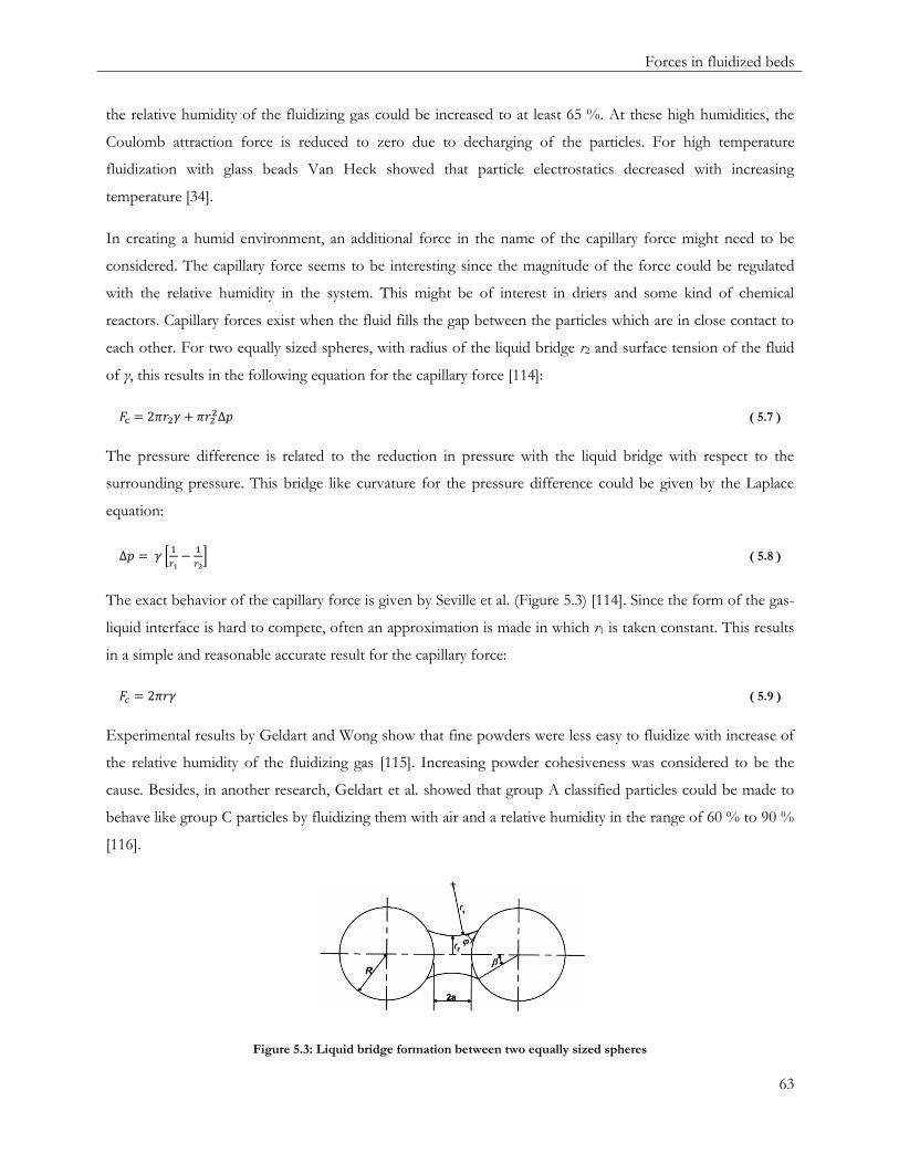
Forces in fluidized beds
63
the relative humidity of the fluidizing gas could be increased to at least 65 %. At these high humidities, the
Coulomb attraction force is reduced to zero due to decharging of the particles. For high temperature
fluidization with glass beads Van Heck showed that particle electrostatics decreased with increasing
temperature [34].
In creating a humid environment, an additional force in the name of the capillary force might need to be
considered. The capillary force seems to be interesting since the magnitude of the force could be regulated
with the relative humidity in the system. This might be of interest in driers and some kind of chemical
reactors. Capillary forces exist when the fluid fills the gap between the particles which are in close contact to
each other. For two equally sized spheres, with radius of the liquid bridge r2 and surface tension of the fluid
of γ, this results in the following equation for the capillary force [114]:
( 5.7 )
The pressure difference is related to the reduction in pressure with the liquid bridge with respect to the
surrounding pressure. This bridge like curvature for the pressure difference could be given by the Laplace
equation:
( 5.8 )
The exact behavior of the capillary force is given by Seville et al. (Figure 5.3) [114]. Since the form of the gas-
liquid interface is hard to compete, often an approximation is made in which r1 is taken constant. This results
in a simple and reasonable accurate result for the capillary force:
( 5.9 )
Experimental results by Geldart and Wong show that fine powders were less easy to fluidize with increase of
the relative humidity of the fluidizing gas [115]. Increasing powder cohesiveness was considered to be the
cause. Besides, in another research, Geldart et al. showed that group A classified particles could be made to
behave like group C particles by fluidizing them with air and a relative humidity in the range of 60 % to 90 %
[116].
Figure 5.3: Liquid bridge formation between two equally sized spheres

64
Each of the single interparticle forces mentioned above is rather complicated to understand and difficult to
be qualified. Some of the researchers referred to in this chapter tried to apply the knowledge of the
interparticle forces discussed in this work to changing hydrodynamics at high temperature fluidization, but
without any success. The question arises why these researchers have not first investigated the nature of
interparticle forces in fluidization at room temperature. As could be seen in Chapter 3 and Chapter 4 is
fluidized bed porosity and behavior greatly influenced by particle properties. The influence of interparticle
forces on particles having different properties might be the key in explaining the hydrodynamics in fluidized
beds.
5.2 Discrete particle model
In order to investigate whether interparticle forces might play a role in fluidization under different conditions,
hydrodynamics of gas-solid fluidized beds will be investigated using the discrete particle model (DPM). In
DPM, particles in a fluidized bed are tracked according to Newton’s second law. The total force acting on the
particles could be split up in the external and contact force, of which the external force consists of the
gravitational forces, the pressure gradient in the gas phase and the drag force exerted by the gas. The contact
force, in its turn, is the sum of all the individual contact forces exerted on particles in contact with each other.
One could make use of a hard sphere model or soft sphere model to describe the particle collisions. A good
description of the DPM is given by Laverman [117]. Equations reported by Laverman have been
implemented in the DPM model used.
In this work, DPM will be used in order to verify whether particle properties influence the fluidization
behavior, and especially the porosity at minimum fluidization. Differently sized particles will be used in order
to check its influence on the fluidized bed porosity. As mentioned, DPM takes into account the gravitational
and drag forces acting on particle beds, but does not account for the interparticle forces. In case any
variations between experiments and DPM simulations are found, interparticle forces are likely to play a big
role in explaining fluidization at room temperature. Moreover, this could mean that the explanation for high
temperature fluidization is related to changing interparticle forces as well.
On overview of the settings used in the DPM simulations is given in Table 5.1.
5.3 Results and discussion
DPM simulations for the different settings shown in Table 5.1 have run for different gas flow rates. Just as
for the determination of the average bed porosity with digital image analysis (DIA), the total bed height is
used and correlated to the porosity by the total number of particles and particle density. It should be noted
that the simulation with 250 μm and helium is still running, since the simulations with helium require a
smaller time step. Simulations with even smaller particles have been started, but because of a relative large
domain to overcome wall effects, these simulations have to date not been finished.
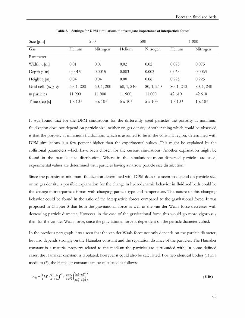
Forces in fluidized beds
65
Table 5.1: Settings for DPM simulations to investigate importance of interparticle forces
Size [μm] 250 500 1 000
Gas Helium Nitrogen Helium Nitrogen Helium Nitrogen
Parameter
Width x [m] 0.01 0.01 0.02 0.02 0.075 0.075
Depth y [m] 0.0015 0.0015 0.003 0.003 0.063 0.0063
Height z [m] 0.04 0.04 0.08 0.06 0.225 0.225
Grid cells (x, y, z) 50, 1, 200 50, 1, 200 60, 1, 240 80, 1, 240 80, 1, 240 80, 1, 240
# particles 11 900 11 900 11 900 11 000 42 610 42 610
Time step [s] 1 x 10⁻⁵ 5 x 10⁻⁵ 5 x 10⁻⁵ 5 x 10⁻⁵ 1 x 10⁻⁴ 1 x 10⁻⁴
It was found that for the DPM simulations for the differently sized particles the porosity at minimum
fluidization does not depend on particle size, neither on gas density. Another thing which could be observed
is that the porosity at minimum fluidization, which is assumed to be in the constant region, determined with
DPM simulations is a few percent higher than the experimental values. This might be explained by the
collisional parameters which have been chosen for the current simulations. Another explanation might be
found in the particle size distribution. Where in the simulations mono-dispersed particles are used,
experimental values are determined with particles having a narrow particle size distribution.
Since the porosity at minimum fluidization determined with DPM does not seem to depend on particle size
or on gas density, a possible explanation for the change in hydrodynamic behavior in fluidized beds could be
the change in interparticle forces with changing particle type and temperature. The nature of this changing
behavior could be found in the ratio of the interparticle forces compared to the gravitational force. It was
proposed in Chapter 3 that both the gravitational force as well as the van der Waals force decreases with
decreasing particle diameter. However, in the case of the gravitational force this would go more vigorously
than for the van der Waals force, since the gravitational force is dependent on the particle diameter cubed.
In the previous paragraph it was seen that the van der Waals force not only depends on the particle diameter,
but also depends strongly on the Hamaker constant and the separation distance of the particles. The Hamaker
constant is a material property related to the medium the particles are surrounded with. In some defined
cases, the Hamaker constant is tabulated; however it could also be calculated. For two identical bodies (1) in a
medium (3), the Hamaker constant can be calculated as follows:
( 5.10 )
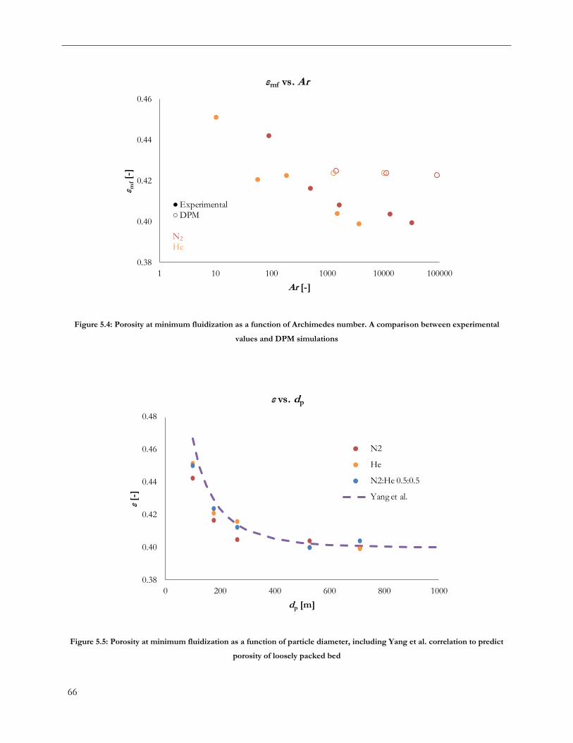
66
0.38
0.40
0.42
0.44
0.46
1 10 100 1000 10000 100000
ε mf[-
]
Ar [-]
εmf vs. Ar
● Experimental
○ DPM
N2
He
Figure 5.4: Porosity at minimum fluidization as a function of Archimedes number. A comparison between experimental
values and DPM simulations
0.38
0.40
0.42
0.44
0.46
0.48
0 200 400 600 800 1000
ε[-
]
dp [m]
ε vs. dp
N2
He
N2:He 0.5:0.5
Yang et al.
Figure 5.5: Porosity at minimum fluidization as a function of particle diameter, including Yang et al. correlation to predict
porosity of loosely packed bed
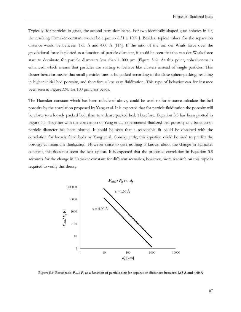
Forces in fluidized beds
67
Typically, for particles in gases, the second term dominates. For two identically shaped glass spheres in air,
the resulting Hamaker constant would be equal to 6.31 x 10⁻²⁰ J. Besides, typical values for the separation
distance would be between 1.65 Å and 4.00 Å [114]. If the ratio of the van der Waals force over the
gravitational force is plotted as a function of particle diameter, it could be seen that the van der Waals force
start to dominate for particle diameters less than 1 000 μm (Figure 5.6). At this point, cohesiveness is
enhanced, which means that particles are starting to behave like clusters instead of single particles. This
cluster behavior means that small particles cannot be packed according to the close sphere packing, resulting
in higher initial bed porosity, and therefore a less easy fluidization. This type of behavior can for instance
been seen in Figure 3.9b for 100 μm glass beads.
The Hamaker constant which has been calculated above, could be used to for instance calculate the bed
porosity by the correlation proposed by Yang et al. It is expected that for particle fluidization the porosity will
be closer to a loosely packed bed, than to a dense packed bed. Therefore, Equation 5.5 has been plotted in
Figure 5.5. Together with the correlation of Yang et al., experimental fluidized bed porosity as a function of
particle diameter has been plotted. It could be seen that a reasonable fit could be obtained with the
correlation for loosely filled beds by Yang et al. Consequently, this equation could be used to predict the
porosity at minimum fluidization. However since to date nothing is known about the change in Hamaker
constant, this does not seem the best option. It is expected that the proposed correlation in Equation 3.8
accounts for the change in Hamaker constant for different scenarios, however, more research on this topic is
required to verify this theory.
1
10
100
1000
10000
100000
1 10 100 1000 10000
Fvd
W/
Fg
[-]
dp [μm]
FvdW/Fg vs. dp
s =1.65 Å
s = 4.00 Å
Figure 5.6: Force ratio Fvdw/Fg as a function of particle size for separation distances between 1.65 Å and 4.00 Å
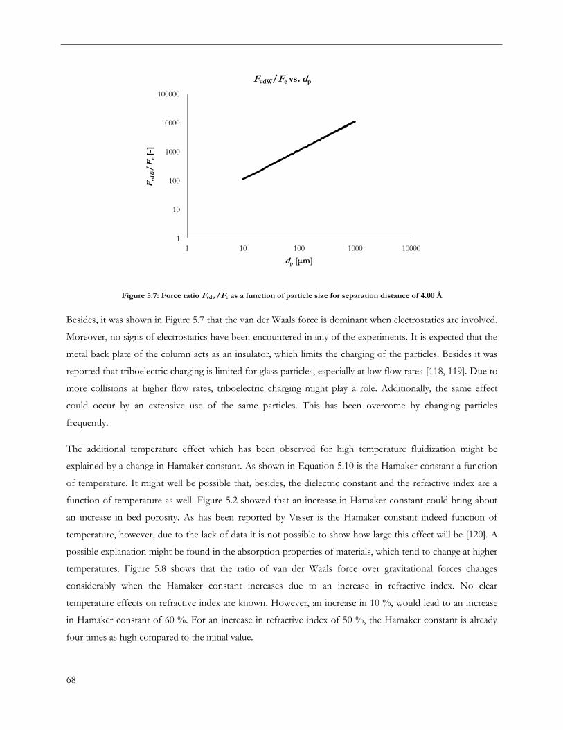
68
1
10
100
1000
10000
100000
1 10 100 1000 10000
Fvd
W/
Fe[-
]
dp [μm]
FvdW/Fe vs. dp
Figure 5.7: Force ratio Fvdw/Fe as a function of particle size for separation distance of 4.00 Å
Besides, it was shown in Figure 5.7 that the van der Waals force is dominant when electrostatics are involved.
Moreover, no signs of electrostatics have been encountered in any of the experiments. It is expected that the
metal back plate of the column acts as an insulator, which limits the charging of the particles. Besides it was
reported that triboelectric charging is limited for glass particles, especially at low flow rates [118, 119]. Due to
more collisions at higher flow rates, triboelectric charging might play a role. Additionally, the same effect
could occur by an extensive use of the same particles. This has been overcome by changing particles
frequently.
The additional temperature effect which has been observed for high temperature fluidization might be
explained by a change in Hamaker constant. As shown in Equation 5.10 is the Hamaker constant a function
of temperature. It might well be possible that, besides, the dielectric constant and the refractive index are a
function of temperature as well. Figure 5.2 showed that an increase in Hamaker constant could bring about
an increase in bed porosity. As has been reported by Visser is the Hamaker constant indeed function of
temperature, however, due to the lack of data it is not possible to show how large this effect will be [120]. A
possible explanation might be found in the absorption properties of materials, which tend to change at higher
temperatures. Figure 5.8 shows that the ratio of van der Waals force over gravitational forces changes
considerably when the Hamaker constant increases due to an increase in refractive index. No clear
temperature effects on refractive index are known. However, an increase in 10 %, would lead to an increase
in Hamaker constant of 60 %. For an increase in refractive index of 50 %, the Hamaker constant is already
four times as high compared to the initial value.
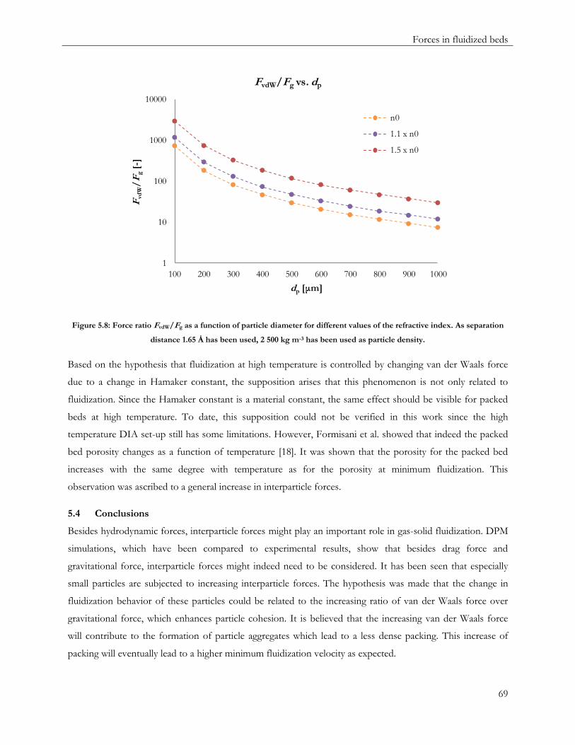
Forces in fluidized beds
69
1
10
100
1000
10000
100 200 300 400 500 600 700 800 900 1000
Fvd
W/
Fg
[-]
dp [μm]
FvdW/Fg vs. dp
n0
1.1 x n0
1.5 x n0
Figure 5.8: Force ratio FvdW/Fg as a function of particle diameter for different values of the refractive index. As separation
distance 1.65 Å has been used, 2 500 kg m-3 has been used as particle density.
Based on the hypothesis that fluidization at high temperature is controlled by changing van der Waals force
due to a change in Hamaker constant, the supposition arises that this phenomenon is not only related to
fluidization. Since the Hamaker constant is a material constant, the same effect should be visible for packed
beds at high temperature. To date, this supposition could not be verified in this work since the high
temperature DIA set-up still has some limitations. However, Formisani et al. showed that indeed the packed
bed porosity changes as a function of temperature [18]. It was shown that the porosity for the packed bed
increases with the same degree with temperature as for the porosity at minimum fluidization. This
observation was ascribed to a general increase in interparticle forces.
5.4 Conclusions
Besides hydrodynamic forces, interparticle forces might play an important role in gas-solid fluidization. DPM
simulations, which have been compared to experimental results, show that besides drag force and
gravitational force, interparticle forces might indeed need to be considered. It has been seen that especially
small particles are subjected to increasing interparticle forces. The hypothesis was made that the change in
fluidization behavior of these particles could be related to the increasing ratio of van der Waals force over
gravitational force, which enhances particle cohesion. It is believed that the increasing van der Waals force
will contribute to the formation of particle aggregates which lead to a less dense packing. This increase of
packing will eventually lead to a higher minimum fluidization velocity as expected.
70
The change in fluidization behavior at high temperature is also expected to be related to changing van der
Waals force. The Hamaker constant, which determines the degree of the van der Waals force, is expected to
increase with temperature, which increases the ratio of van der Waals force over gravitational force. This
means that for particles of the same size, a more cohesive character is expected, leading to a larger porosity
and less easy fluidization.

Conclusion and recommendations
71
Conclusion and recommendations
Predicting the behavior of fluidized beds is a challenging task. In this report, it has been seen that many
correlations to predict the minimum fluidization velocity are available, but none of them are applicable for a
wide range of conditions. Most of them are based on the Ergun equation and make use of the approach by
Wen & Yu to correlate particle sphericity and porosity at minimum fluidization. Others are purely empirical,
and based on a limited set of experimental data. In engineering applications, often the minimum fluidization
velocity is predicted at room temperature and corrected for the change in density and viscosity at high
temperature. In this work it was shown that this procedure is not valid and will often lead to a reactor design
which is far from optimum.
It was shown that one of the key factors, which is often assumed to be constant, is the porosity at minimum
fluidization. Different factors, like particle properties, gas properties and temperature, tend to influence the
porosity and therefore fluidization behavior. A correlation has been proposed to predict the porosity at
minimum fluidization within 3 % error for different types of spherical particles. This will eventually lead to a
predictive error of maximum 10 % in the Reynolds number at minimum fluidization, based on the Carman-
Kozeny equation.

72
Hydrodynamics of bubbling fluidized beds of differently sized particles have been studied with digital image
analysis (DIA) and compared to each other. Since the excess gas velocity was kept constant in all cases,
comparable bubble sizes should be expected based on the correlation proposed by Shen et al. However, since
particle beds with smaller particles allow more gas to pass the emulsion phase, bubble size was shown to be
smaller in such systems. It is assumed that this phenomenon could be corrected for by considering the visual
bubble flow rate, which is defined as the gas which passes the bed as bubble compared to the total excess gas.
A possible explanation for the observed behavior in fluidized beds is related to the changing van der Waals
force in different conditions. Discrete particle model (DPM) simulations suggest that beside drag force and
gravitational force, interparticle forces might play a role. For smaller particles, it was shown that the van der
Waals force dominates over the gravitational force, which influences the packing behavior of the particles. It
is assumed that particles start to behave like aggregates due to the cohesive behavior of the van der Waals
force. The additional temperature effect is likely to be found in the temperature dependence on the Hamaker
constant, which was shown to have a clear effect on particle packing. Nonetheless, to date, very little is
known about the exact temperature effect on the Hamaker constant.
Additional steps could be taken in order to further improve this work. First of all, it is advisable to determine
the exact sphericity of the particles used. Till now, it has been assumed that the glass particles used are
perfectly spherical; however, it could be possible that in practice their sphericity is less than unity. It has been
seen that the sphere factor has a major influence on the particle packing, resulting in a different porosity.
Besides, particles having different sphere factors could extend the usage of the proposed correlation. It is
advised to experimentally determine the porosity for more different particles, so a relation to account for the
sphericity could be included. Moreover, it might be interesting to see how non-spherical particles behave at
high temperature.
As soon as the high temperature set-up is fully operatable, hydrodynamics at high temperature can be studied.
It should be noted that possibly changes have to be made in the DIA code, since different bubbling behavior
is expected at high temperature. Besides, the effect of temperature on the porosity of both packed bed as well
as fluidized bed can be studied visually.
To get a better fundamental understanding in the hydrodynamics of fluidized beds and factors affecting
fluidization behavior, the DPM study could be extended. Firstly, it is advised to study the influence of the
collision parameters on the simulation results. Besides, a good idea would be to incorporate interparticle
forces in the model as well. As soon as this has been done, DPM simulations can be compared to the real
experimental behavior which is observed in the high temperature set-up.

References
73
References
[1] S. Shafiee and E. Topal, "When will fossil fuel reserves be diminished?," Energy Policy, vol. 37, pp. 181-
189, 2009.
[2] G. Chen, J. Andries and H. Spliethoff, "Biomass conversion into fuel gas using circulating fluidised bed
technology: the concept improvement and modelling discussion," Renewable Energy, vol. 28, pp. 985-994,
2003.
[3] I. Catic and M. Rujnic-Sokele, "Agriculture products - Food for living beings of machinery?," Gummi,
Fasern, Kunstoffe, vol. 61, pp. 701-708, 2008.
[4] P. Hellegers, D. Zilbermann, P. Stedto and P. McCornick, "Interactions between water, energy, food
and environment: evolving perspectives and policy issues," Water Policy, vol. 10, pp. 1-10, 2008.
[5] G. Stoeglehner and M. Narodoslawsky, "How sustainable are biofuels? Answers and further quesions

74
arising from an ecological footprint perspective," Bioresource Technology, vol. 100, pp. 3825-3830, 2009.
[6] S. Majhi, P. Mohanty, H. Wang and K. Pant, "Direct conversion of natural gas to higher hydrocarbons:
A review," Journal of Energy Chemistry, vol. 22, pp. 543-554, 2013.
[7] C. Van der Meijden, L. Rabou, A. Van der Drift, B. Vreugdenhil and R. Smit, "Large scale production
of bio methane from wood," in International Gas Union Research Conference, Seoul, 2011.
[8] C. Van der Meijden, A. Van der Drift and B. Vreugdenhil, "Benefits of allothermal biomass gasification
for co-firing," in 2nd Workshop on cofiring biomass with coal, Copenhagen, 2012.
[9] A. Arbel, Z. Huang, I. H. Rinard, R. Shinnar and A. V. Sapre, "Dynamic and control of luidized
catalytic crackers. 1. Modeling of the current generation of FCC's," Industrial & Engineering Chemical
Research, vol. 34, pp. 1228-1243, 1995.
[10] J. C. Abanades, E. J. Anthony, J. Wang and J. E. Oakey, "Fluidized bed combustion systems
integrationg CO2 capture with CaO," Environmental Science & Technology, vol. 39, pp. 2861-2866, 2005.
[11] I. Burdett, R. Eisinger, P. Kai and K. Lee, "Gas-Phase fluidization technology for production of
polyolefins," in Fluidization X, New York, 2001.
[12] D. Kunii and O. Levenspiel, Fluidization Engineering, 2nd edition, Butterworth-Heinemann, 1991.
[13] S. Sanaei, N. Mostoufi, R. Radmanesh, R. Sotudeh-Gharebagh and J. Chaouki, "Effect of temperature
on hydrodynamics of fluidized beds," in Proceedings of European Congress of Chemical Engineering (ECCE-6),
Copenhagen, 2007.
[14] J.-H. Choi, H.-J. Ryu, D.-W. Shun, J.-E. Son and S.-D. Kim, "Temperature effect on the particle
entrainment rate in a gas fluidized bed," Industrial & Engineering Chemical Research, vol. 37, pp. 1130-1135,
1998.
[15] Q. Guo, G. Yue, T. Suda and J. Sato, "Flow characteristics in a bubbling fluidized bed at elevated
temperature," Chemical Engineering and Processing, vol. 42, pp. 439-447, 2003.
[16] K. Svoboda and M. Hartman, "Influence of temperature on inciptent fluidization of limeston, lime, coal
ash, and corundum," Industrial & Engineering Chemistry Process Design and Development, vol. 20, no. 1981, pp.
319-326, 1981.
References
75
[17] H. Cui, P. Sauriol and J. Chaouki, "High temperature fluidized bed reactor: measurements,
hydrodynamics and simulation," Chemical Engineering Science, vol. 58, pp. 1071-1077, 2003.
[18] B. Formisani, R. Girimonte and G. Pataro, "The influence of operating temperature on the dense phase
properties of bubbling fluidized beds of solids," Powder Technology, vol. 125, pp. 28-38, 2002.
[19] B. Formisani, R. Girimonte and L. Mancuso, "Analysis of the fluidization process of particle beds at
high temperature," Chemical Engineering Science, vol. 53, pp. 951-961, 1998.
[20] G. Raso, M. D. Amore, B. Formisani and P. Lignola, "The influence of temperature on the properties
of the particulate phase at incipent fluidization," Powder Technology, vol. 72, pp. 71-76, 1992.
[21] P. Lettieri, J. Yates and D. Newton, "The influence of interparticle forces on the fluidization behavior
of some industrial materials at high temperature," Powder Technology, vol. 110, pp. 117-127, 2000.
[22] M. Poletto, P. Salatino and L. Massimilla, "Fluidization of solids with CO2 at pressures and
temperatures from ambient to nearly critical conditions," Chemical Engineering Science, vol. 48, pp. 617-
621, 1993.
[23] K. Rietema and H. Piepers, "The effect of interparticle forces on the stability of gas-fluidized beds - 1.
Experimental evidence," Chemical Engineering Science, vol. 45, pp. 1627-1639, 1990.
[24] L. Massimilla and G. Donsi, "Cohesive forces between particles of fluid-bed catalysts," Powder Technology,
vol. 15, pp. 253-260, 1976.
[25] C. Boyer, A. Duquenne and G. Wild, "Measuring techniques in gas-liquid and gas-liquid-solid reactors,"
Chemical Engineering Science, vol. 57, pp. 3185-3215, 2002.
[26] R. Adrian, "Scattering particle characteristics and their effect on pulsed laser measurements of fluid
flow: speckle velocimetry vs particle image velocimetry," Applied Optics, vol. 23, pp. 1690-1691, 1984.
[27] R. Adrian, "Twenty years of particle image velocimetry," Experiments in Fluids, vol. 39, pp. 159-169,
2005.
[28] R. Adrian and J. Westerweel, Particle Image Velocimetry, Cambridge University Press, 2011.
[29] J. Laverman, I. Roghair, M. Van Sint Annaland and H. Kuipers, "Investigation into the hydrodynamics
of gas-solid fluidized beds using particle image velocimetry coupled with digital image analysis," The

76
Canadian Journal of Chemical Engineering, vol. 86, pp. 523-535, 2008.
[30] J. Link, C. Zeilstra, N. Deen and J. Kuipers, "Validation of a discrete particle model in a 2D spout-fluid
bed using non-intrusive optical measuring techniques," The Canadian Journal of Chemical Engineering, vol.
82, pp. 30-36, 2004.
[31] N. Deen, M. Van Sint Annaland and J. Kuipers, "Detailed computational and experimental fluid
dynamics of fluidized beds," Applied Mathematical Modelling, vol. 30, pp. 1459-1471, 2006.
[32] M. Van Buijtenen, M. Bomer, N. Deen, S. Heinrich, S. Antonyuk and J. Kuipers, "An experimental
study of the effect of collision properties on spout fluidized bed dynamics," Powder Technology, vol. 206,
pp. 139-148, 2011.
[33] J. De Jong, S. Odu, M. Van Buijtenen, N. Deen, M. Van Sint Annaland and J. Kuipers, "Development
and validation of a novel digital image analysis method for fluidized bed particle image velocimetry,"
Powder Technology, vol. 230, pp. 193-202, 2012.
[34] L. Van Heck, "An experimental study of the hydrodynamics in fluidized bed reactors," Eindhoven
University of Technology, 2012.
[35] U. Dierkshelde, P. Meyer, T. Hovestadt and W. Hentschel, "Endoscopic 2D particle image velocimetry
(PIV) flow field measurements in IC engines," Experiments in Fluids, vol. 33, pp. 794-800, 2002.
[36] E. Delnoij, J. Kuipers, W. Van Swaaij and J. Westerweel, "Measurement of gas-liquid two-phase flow in
bubble colum using ensemble correlation PIV," Chemical Engineering Science, vol. 55, pp. 3385-3395, 2000.
[37] S. Van Belzen, "Hydrodynamics of fluidized beds under reactive conditions," Eindhoven University of
Technology, 2013.
[38] R. Girimonte and B. Formisani, "The minimum bubbling velocity of fluidized beds operating at high
temperature," Powder Technology, vol. 189, pp. 74-81, 2009.
[39] R. Pattipati and C. Wen, "Minimum fluidization velocity at high temperatures," Industrial & Engineering
Chemistry Process Design and Development, vol. 20, pp. 705-708, 1981.
[40] J. Botterill, Y. Teoman and K. Yuregir, "The effect of operating temperature on the velocity of
minimum fluidization," Powder Technology, vol. 31, pp. 101-110, 1982.

References
77
[41] S. Rapagna, P. Foscolo and L. Gibilaro, "The influence of temperature on the quality of gas
fluidization," International Journal of Multiphase Flow, vol. 20, pp. 305-313, 1994.
[42] H. Xie and D. Geldart, "Fluidization of FCC powders in the bubble-free regime: effect of type of gases
and temperature," Powder Technology, vol. 82, pp. 269-277, 1995.
[43] J. Baeyens and D. Geldart, "Predictive calculations of flow parameters in gas fluidised beds and
fluidisation behaviour of various powders," in Proc. Conf. La Fluidisation et ses Applications, Toulouse,
1973.
[44] C. Wen and Y. Yu, "A generalized method for predicting the minimum fluidization velocity," AIChE
journal, vol. 12, pp. 610-612, 1966.
[45] H. Subramani, M. Balaiyya and L. Miranda, "Minimum fluidization velocity at eleveated temperatures
for Geldart's group B powders," ExperimentalThermal and Fluid Science, vol. 32, pp. 166-173, 2007.
[46] A. Lucas, J. Arnaldos, J. Casal and L. Puigjaner, "High temperature incipient fluidization in mono and
poly disperse systems," Chemical Engineering Communications, vol. 41, pp. 121-132, 1986.
[47] E. Johnson, "Publication No. 318/179," Institute of Gas Engineers Report, 1949-50.
[48] C. Miller and A. Logwinuk, "Fluidization studies of solid particles," Industrial Engineering Chemistry, vol.
43, pp. 1220-1226, 1951.
[49] C. Van Heerden, A. Nobel and D. Van Krevelen, "Studies on fluidization I - the critical mass velocity,"
Chemical Engineering Science, vol. 1, pp. 37-49, 1951.
[50] S. Ergun, "Fluid flow through parcked columns," Chemical Engineering Progress , vol. 48, pp. 89-94, 1952.
[51] M. Leva, T. Shirai and C. Wen, "Prediction of onset fluidzation in beds of granular solids," Genie
Chimique, vol. 75, p. 33, 1956.
[52] O. Todes, V. Goroshkov and R. Rozenbaum, Izv. Vyssh. Uchcbn. Zaved. Neft Gaz, vol. 1, p. 8, 1958.
[53] M. Leva, Fluidization, New York: McGraw Hill, 1959.
[54] K. Andersson, "Pressure drop in ideal fluidization," Chemical Engineering Science, vol. 15, pp. 276-297,
1961.
78
[55] P. Rowe and G. Henwood, "Drag forces in a hydraulic model on a fluidised bed - Part I," Transactions of
the Institution of Chemical Engineers, vol. 39, pp. 43-54, 1961.
[56] G. Narsimham, "On generalized expression for prediction of minimum fluidization velocity," AIChE
Journal, vol. 11, pp. 550-554, 1965.
[57] J. Frantz, "Minimum fluidization velocities and pressure in fluidized beds," Chemical Engineering Progress
Smposium Series, vol. 62, pp. 21-31, 1966.
[58] C. Wen and Y. Yu, "Mechanics of fluidization," Chemical Engineering Progress Symposium Series, vol. 62, pp.
100-11, 1966.
[59] V. Goroshko, R. Rozenbaum and O. Todes, "Hydrodynamics and heat transfer in fluidized beds," MIT
Press, pp. 71-73, 1966.
[60] L. Davies and J. Richardson, "Gas interchange between bubbles and the continuous phase in a fluidized
bed," Transaction of Institution of Chemical Engineers, vol. 44, pp. 293-305, 1966.
[61] J. H. J. Bena, "Determination of minimum fluidization velocity of polydispersed materials (2)," Chemicke
Zvesti, vol. 21, p. 877, 1967.
[62] P. Bourgeis and P. Genier, "Ratio of terminal velocity to minimum fluidization velocity for spherical
particles," Canadian Journal of Chemical Engineering, vol. 46, pp. 325-328, 1968.
[63] C. Pillai and M. Raja Rao, Indian Journal of Technology, vol. 9, p. 77, 1971.
[64] W. Goosens, G. Dumont and G. Spaepen, "Fluidization of binary mixture in the laminar flow region,"
Chemical Engineering Progress Symposium Series, vol. 67, pp. 38-45, 1971.
[65] A. Kumar and P. Sen Gupta, "Predictive culculations of minimum fluidization velocity for
multicomponent mixtures," Indian Journal of Technology, vol. 12, pp. 225-228, 1974.
[66] T. Broadhurst and H. Becker, "Onset of fluidization and slugging in beds of uniform particles," AIChE
Journal, vol. 21, pp. 238-247, 1975.
[67] G. Davtyan, V. Ainshtein and R. Grigoryan, Izv. Akd. Nauk, Arm. SSr, Ser. Tekh. Nauk , vol. 26, p. 36,
1976.

References
79
[68] S. Saxena and G. Vogel, "The measurement of incipient fluidization velocities in a bed course dolomite
at temperature and pressure," Transaction of Institution of Chemical Engineers, vol. 55, pp. 184-189, 1977.
[69] S. Babu, B. Shah and A. Talwalker, "Fluidization correlations for coal gasification materials - minimum
fluidzation velocity and fluidized bed expansion ratio," Chemical Engineering Progress Symposium Series, vol.
74, pp. 176-186, 1978.
[70] J. Riba, R. Routie and J. Couderc, "Minimum conditions for fluidisation bya a liquid," Canadian Journal of
Chemical Engineering, vol. 56, pp. 26-30, 1978.
[71] R. Vaid and P. Sen Gupta, "Minimum fluidization velocities in beds of mixtures," Canadian Journal of
Chemical Engineering, vol. 56, pp. 292-296, 1978.
[72] A. Doichev and N. Akhmakov, "Fluidization of polydisperse systems," Chemical Engineering Science, vol.
34, pp. 1357-1359, 1979.
[73] J. Richardson and M. Jeromino, "Velocity voidage relations for sedimentation and fluidization," Chemical
Engineering Science, vol. 34, pp. 1419-1422, 1979.
[74] V. Thonglimp, N. Hiquily and C. Laguerie, "Vitesse minimale de fluidisation et expansion des couches
fluidisees par un gas," Powder Technology, vol. 39, pp. 233-253, 1984.
[75] J. Grace, Handbook of Multiphase Systems, Washington: Hemisphere Pub. Corp., 1982.
[76] D. Chitester, "Characteristics of fluidization at high pressure," Chemical Engineering Science, vol. 39, p. 253,
1984.
[77] Z. Zheng, R. Yamazaki and G. Jimbo, "Minimum fluidization velocity of large particles at elevated
temperatures," Kagaku Kogaku Ronbunsha, vol. 11, p. 115, 1985.
[78] V. Thonglimp, Fluidization, London: Academic Press, 1985.
[79] C. Chyang and W. Huang, "Characteristics of large particle fluidization," Journal of The Chnese Institution of
Chemical Engineers, vol. 19, pp. 81-89, 1988.
[80] K. Sathyanarayana and P. Rao, "Minimum fluidization at elevated temperatures," Indian Chemical
Engineering, vol. 31, pp. 79-81, 1989.
80
[81] S. Wu and J. Baeyens, "Effect of operating temperature on minimum fluidization velocity," Powder
Technology, vol. 67, pp. 217-220, 1991.
[82] N. Fatah, "Theses de doctorat," INP-Toulouse, 1991.
[83] J. Adanez and J. Abanades, "Minimum fluidization velocities of fluidized-bed coal-combustion solids,"
Powder Technology, vol. 67, pp. 113-119, 1991.
[84] J. Fletcher, M. Deo and F. Hanson, "Re-examination of minimum fluidization velocity correlations
applied to Group B sands and coked sands," Powder Technology, vol. 69, pp. 147-155, 1992.
[85] M. Mourad, M. Hemati and C. Laguerie, "Hydrodynamics d'un sechoir a' lit fluidise a'flottation:
determination des vitesses caracteristiques de fluidisation de melanges de mais et de sable," Powder
Technology, vol. 80, pp. 45-54, 1194.
[86] K. Tannous, M. Hemati and C. Laguerie, "Caracteristiques au minimum de fluidisation et expansion des
couches fluidisees de particules de la categorie D de Geldart," Powder Technology, vol. 80, pp. 55-72, 1994.
[87] A. Bin, "Prediction of the minimum fluidization velocity," Powder Technology, vol. 81, pp. 197-199, 1994.
[88] D. Barbosa, D. Steinmetz and H. Angelino, "Fluidization VIII," LagueArie adn Large, vol. 1, pp. 145-153,
1995.
[89] D. Gauthier, S. Zerguerras and G. Flamant, "Influence of the particle size distribution of powders of
the velocities of minimum and complete fluidization," Chemical Engineering Journal, vol. 74, pp. 181-196,
1999.
[90] J. Reina, E. Velo and L. Puigjaner, "Predicting the minimum fluidization velocity of polydisperse
mixtures of scrap-wood partciles," Powder Technology, vol. 111, pp. 245-251, 2000.
[91] M. Hartman, O. Trnka and K. Svoboba, "Fluidization characteristics of dolomite and calcined dolomite
particles," Chemical Engineering Science, vol. 55, pp. 6269-6274, 2000.
[92] A. Delebarre, "Rivisiting the Wen and Yu equations for minimum fluidization velocity prediction,"
Chemical Engineering Research and Design, vol. 82, pp. 587-590, 2004.
[93] R. Coltters and A. Rivas, "Minimum fluidization velocity correlations in particulate systems," Powder
References
81
Technology, vol. 147, pp. 34-48, 2004.
[94] Z. Zhiping, N. Yongjie and L. Qinggang, "Effect of pressure on minimum fluidization velocity," Journal
of Thermal Science, vol. 16, pp. 264-269, 2007.
[95] E. Rabinovich and H. Kalman, "Generalized master curve for threshold superficial velocities in particle
- fluid systems," Powder Technology, vol. 183, pp. 304-313, 2008.
[96] B. Paudel and Z. Feng, "Prediction of minimum fluidization velocity for binary mixtures of biomass
and inert particles," Powder Technology, vol. 237, pp. 134-140, 2013.
[97] I. Puspasari, M. Talib, W. Daud and S. Tasirin, "Fluidization characteristics of oil palm frond particles in
agitated bed," Chemical Engineering Research and Design, vol. 91, pp. 497-507, 2013.
[98] A. Mathur, S. Saxena and Z. Zhand, "Hydrodynamic characteristics of gas-fluidized beds over a broad
temperature range," Powder Technology, vol. 47, pp. 247-256, 1986.
[99] A. Yu and N. Standish, "Characterisation of non-spherical particles from their packing behaviour,"
Powder Technology, vol. 74, pp. 205-213, 1993.
[100] R. Toomey and H. Johnstone, "Gaseous fluidization of solid particles," Chemical Engineering Progress, vol.
48, p. 200, 1952.
[101] J. Davidson and D. Harrison, Fluidized Particles, New York: Cambridge University Press, 1963.
[102] L. Shen, F. Johnsson and B. Leckner, "Digital image analysis of hydrodynamics two-dimensional
bubbling fluidized beds," Chemical Engineering Science, vol. 59, pp. 2607-2617, 2004.
[103] J. Werther, "Effect of gas distribution on the hydrodynamics of gas fluidized beds," German Chemical
Engineering, vol. 1, p. 166, 1978.
[104] R. Mudde, H. Schulte and H. Van den Akker, "Analysis of a bubbling 2-D gas-fluidized bed using image
processing," Powder Technology, vol. 81, pp. 149-159, 1994.
[105] K. Hilligardt and J. Werther, "Local bubble gas hold-up and expansion of gas/solid fluidized beds,"
German Chemical Engineering, vol. 6, p. 215, 1986.
[106] H. Cui and J. Chaouki, "Interparticle forces in high temperature fluidization of Geldart A particles,"

82
China Particuology, vol. 2, pp. 113-118, 2004.
[107] D. Geldart, "Types of gas fluidization," Powder Technology, vol. 7, pp. 285-292, 1973.
[108] J. Visser, "Van der Waals and other cohesive forces affecting powder fluidization," Powder Technology, vol.
58, pp. 1-10, 2989.
[109] J. Israelachvili, Intermolecular and Surface Forces, London: Academic Press, 1991.
[110] A. Yu, C. Feng, R. Zou and R. Yang, "On the relationship between porosity and interparticle forces,"
Powder Technology, vol. 130, pp. 70-76, 2003.
[111] A. Yu, J. Bridgwater and A. Burbidge, "On the modelling of packing of fine particles," Powder Technology,
vol. 92, pp. 185-194, 1997.
[112] A. Bailey, "Electrostatic phenomna during powder handling," Powder Technology, vol. 37, pp. 71-85, 1984.
[113] W. Schnabel, PhD Thesis, Karlsruhe University, 1969.
[114] J. Seville, C. Willett and P. Knight, "Interparticle forces in fluidisation: a review," Powder Technology, vol.
113, pp. 261-168, 2000.
[115] D. Geldart and C. Wong, "Entrapment of particles from fluidized beds of fine powders D," AIChE
Symposium Series, vol. 83, p. 1, 1987.
[116] D. Geldart, N. Harnby and A. Wong, "Fluidization of cohesive powders," Powder Technology, vol. 37, p.
25, 1984.
[117] J. Laverman, On the hydrodynamics in gas polymerization reactors, Eindhoven: Ipskamp Drukkers
B.V. , 2010.
[118] S. Matsusaka, H. Maruyama, T. Matsuyama and M. Ghadiri, "Triboelectric charging of powders: A
review," Chemical Engineering Science, vol. 65, pp. 5781-5807, 2010.
[119] Y. C. Ahn, D. H. Kim, S. C. Kim, E. G. Hwang, G. T. Kim, H. S. Shin and J. K. Lee, "Measurment and
control of triboelectrically charged silica and glassy carbon partilces," Particulate Science and Technology, vol.
22, pp. 305-320, 2004.

References
83
[120] J. Visser, "On Hamaker constants: A comparison between Hamaker constants and Lifshitz - van der
Waals constants," Advances in colloid and interface systems, vol. 3, pp. 331-363, 1972.

84
Appendix 1: Determination of minimum fluidization velocity
85
Appendix 1: Determination of minimum fluidization velocity
The minimum fluidization velocities in this work have been determined by the so-called pressure drop versus
velocity method. In this method, for relatively low flow rates in a fixed bed, the pressure drop increases
proportional to the gas velocity. At a certain gas flow rate, the bed expands and increases the porosity. The
maximum pressure drop is likely to be somewhat higher than the pressure drop resulting from the weight of
the particles. This slight increase in pressure drop is required to go from fixed bed to fluidized bed, which
means that the total bed porosity is increased from the fixed bed porosity to the porosity at minimum
fluidization. At this point, the total drag exerted by the gas equals the gravitational force of the particles.
At gas velocities beyond the minimum fluidization points, the bed starts to expend and particles start to move
around. Increasing the gas flow even further results in the formation of bubbles; this is a result of gas
bypassing the emulsion phase. Even though the gas flow is increased further, the pressure drop will practically
stay at the pressure drop belonging to the static pressure of the bed.
When the gas velocity is decreased, the particles start to settle again to form a loosely packed bed again.
Usually, the minimum fluidization velocity is determined at the intersection point of the trend line of the
defluidization curve with the pressure drop related to the particle weight.
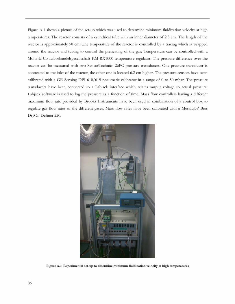
86
Figure A.1 shows a picture of the set-up which was used to determine minimum fluidization velocity at high
temperatures. The reactor consists of a cylindrical tube with an inner diameter of 2.5 cm. The length of the
reactor is approximately 50 cm. The temperature of the reactor is controlled by a tracing which is wrapped
around the reactor and tubing to control the preheating of the gas. Temperature can be controlled with a
Mohr & Co Laborhandelsgesellschaft KM-RX1000 temperature regulator. The pressure difference over the
reactor can be measured with two SensorTechnics 26PC pressure transducers. One pressure transducer is
connected to the inlet of the reactor, the other one is located 6.2 cm higher. The pressure sensors have been
calibrated with a GE Sensing DPI 610/615 pneumatic calibrator in a range of 0 to 50 mbar. The pressure
transducers have been connected to a Labjack interface which relates output voltage to actual pressure.
Labjack software is used to log the pressure as a function of time. Mass flow controllers having a different
maximum flow rate provided by Brooks Instruments have been used in combination of a control box to
regulate gas flow rates of the different gases. Mass flow rates have been calibrated with a MesaLabs' Bios
DryCal Definer 220.
Figure A.1: Experimental set-up to determine minimum fluidization velocity at high temperatures
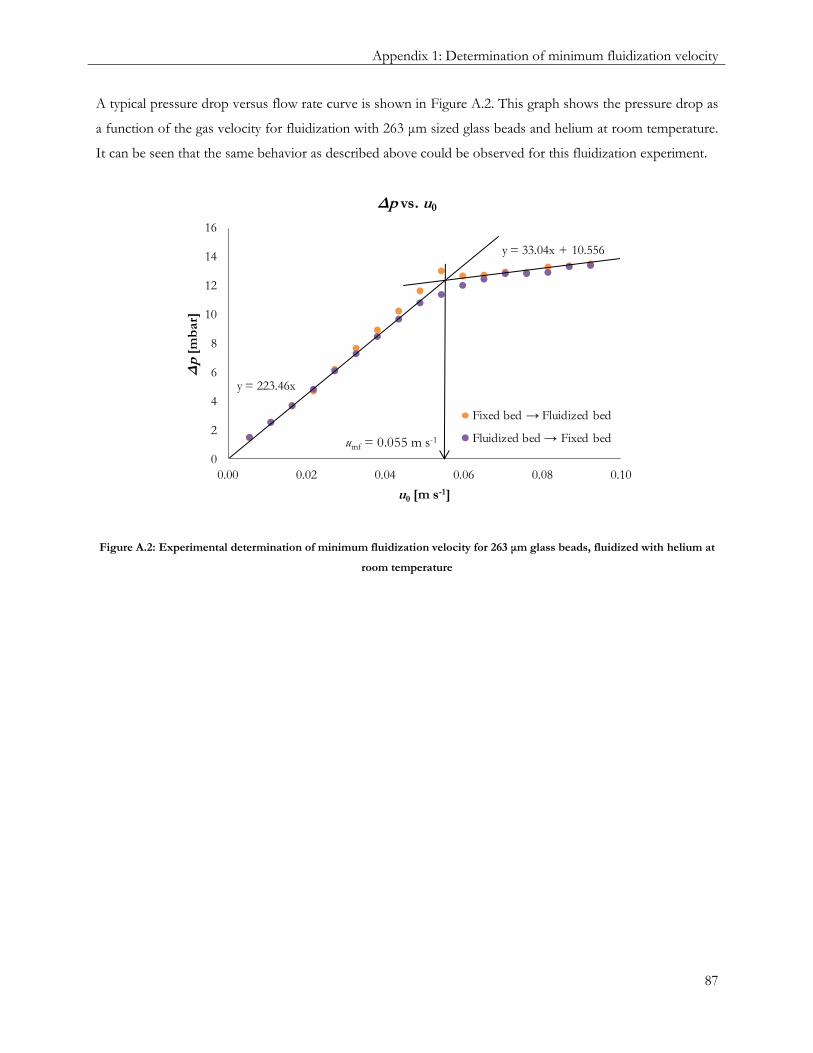
Appendix 1: Determination of minimum fluidization velocity
87
A typical pressure drop versus flow rate curve is shown in Figure A.2. This graph shows the pressure drop as
a function of the gas velocity for fluidization with 263 μm sized glass beads and helium at room temperature.
It can be seen that the same behavior as described above could be observed for this fluidization experiment.
y = 223.46x
y = 33.04x + 10.556
0
2
4
6
8
10
12
14
16
0.00 0.02 0.04 0.06 0.08 0.10
Δp
[mb
ar]
u0 [m s-1]
Δp vs. u0
Fixed bed → Fluidized bed
Fluidized bed → Fixed bedumf = 0.055 m s-1
Figure A.2: Experimental determination of minimum fluidization velocity for 263 μm glass beads, fluidized with helium at
room temperature

88

Appendix 2: Overview of literature values for minimum fluidization porosity for Geldart B particles
89
Appendix 2: Overview of literature values for minimum fluidization porosity for
Geldart B particles
Table A.1: Literature values for minimum fluidization porosity for Geldart B particles
Author
Type
dp [m]
ρp [kg m-3]
Gas
T [°C]
φ [-]
εmf
[-] umf
[m s-1]
Cranfield (1974) aluminium 1 340 1 150 air 20 1.00 0.420 0.560
Cranfield (1974) aluminium 1 340 1 150 air 20 1.00 0.420 0.530
Mathur (1986) sand 751 2 670 air 652 0.75 0.570 0.560
Mathur (1986) sand 559 2 670 air 252 0.84 0.470 0.170
Mathur (1986) sand 559 2 670 air 452 0.83 0.460 0.150
Mathur (1986) sand 751 2 670 air 452 0.72 0.530 0.470
Mathur (1986) sand 751 2 670 air 877 0.70 0.580 0.700
Mathur (1986) sand 1 225 2 670 air 927 0.78 0.530 0.780
Mathur (1986) sand 559 2 670 air 102 0.85 0.460 0.200
Mathur (1986) sand 1 225 2 670 air 727 0.80 0.480 0.800
Mathur (1986) sand 559 2 670 air 777 0.82 0.450 0.140
Mathur (1986) sand 751 2 670 air 227 0.73 0.470 0.450
Mathur (1986) sand 559 2 670 air 927 0.79 0.460 0.130
Mathur (1986) sand 559 2 670 air 27 0.86 0.450 0.220

90
Mathur (1986) sand 1 225 2 670 air 477 0.80 0.440 0.800
Mathur (1986) sand 751 2 670 air 112 0.74 0.400 0.400
Mathur (1986) sand 751 2 670 air 27 0.72 0.430 0.300
Mathur (1986) sand 1 225 2 670 air 227 0.79 0.470 0.790
Mathur (1986) sand 1 225 2 670 air 112 0.81 0.490 0.810
Murachman (1990) corindon 607 3 950 air 20 0.77 0.490 0.550
Murachman (1990) aluminium 917 1 480 air 20 0.92 0.480 0.280
Pattipati (1981) sand 462 2 630 air 281 0.80 0.385 Pattipati (1981) sand 462 2 630 air 391 0.80 0.395 Pattipati (1981) sand 462 2 630 air 18 0.80 0.415 Pattipati (1981) sand 462 2 630 air 551 0.80 0.410 Pattipati (1981) sand 462 2 630 air 611 0.80 0.411 Pattipati (1981) sand 462 2 630 air 625 0.80 0.404 Pattipati (1981) sand 462 2 630 air 786 0.80 0.412 Pattipati (1981) sand 462 2 630 air 921 0.80 0.412 Saxena (1989) glass 147 2 543 air 20 1.00 0.480 0.035
Saxena (1989) glass 423 2 665 air 20 1.00 0.450 0.227
Subramani (2007) ilmenite 128 4 690 air 298 0.73 0.476 0.028
Subramani (2007) ilmenite 128 4 690 air 373 0.73 0.482 0.022
Subramani (2007) ilmenite 128 4 690 air 473 0.73 0.491 0.021
Subramani (2007) ilmenite 128 4 690 air 573 0.73 0.499 0.019
Subramani (2007) ilmenite 128 4 690 air 673 0.73 0.503 0.017
Subramani (2007) ilmenite 128 4 690 air 773 0.73 0.506 0.016
Subramani (2007) ilmenite 128 4 690 air 873 0.73 0.514 0.015
Subramani (2007) ilmenite 128 4 690 air 973 0.73 0.525 0.014
Subramani (2007) ilmenite 163 4 690 air 298 0.73 0.470 0.046
Subramani (2007) ilmenite 163 4 690 air 373 0.73 0.478 0.037
Subramani (2007) ilmenite 163 4 690 air 473 0.73 0.488 0.033
Subramani (2007) ilmenite 163 4 690 air 573 0.73 0.492 0.031
Subramani (2007) ilmenite 163 4 690 air 673 0.73 0.498 0.027
Subramani (2007) ilmenite 163 4 690 air 773 0.73 0.508 0.026
Subramani (2007) ilmenite 163 4 690 air 873 0.73 0.512 0.023
Subramani (2007) ilmenite 163 4 690 air 973 0.73 0.516 0.022
Subramani (2007) ilmenite 200 4 690 air 298 0.73 0.460 0.069
Subramani (2007) ilmenite 200 4 690 air 373 0.73 0.466 0.055
Subramani (2007) ilmenite 200 4 690 air 473 0.73 0.475 0.050
Subramani (2007) ilmenite 200 4 690 air 573 0.73 0.483 0.046
Subramani (2007) ilmenite 200 4 690 air 673 0.73 0.489 0.042
Subramani (2007) ilmenite 200 4 690 air 773 0.73 0.494 0.040
Subramani (2007) ilmenite 200 4 690 air 873 0.73 0.502 0.037
Subramani (2007) ilmenite 200 4 690 air 973 0.73 0.510 0.034
Subramani (2007) sand 200 2 820 air 298 0.67 0.491 0.042
Subramani (2007) sand 200 2 820 air 373 0.67 0.497 0.032
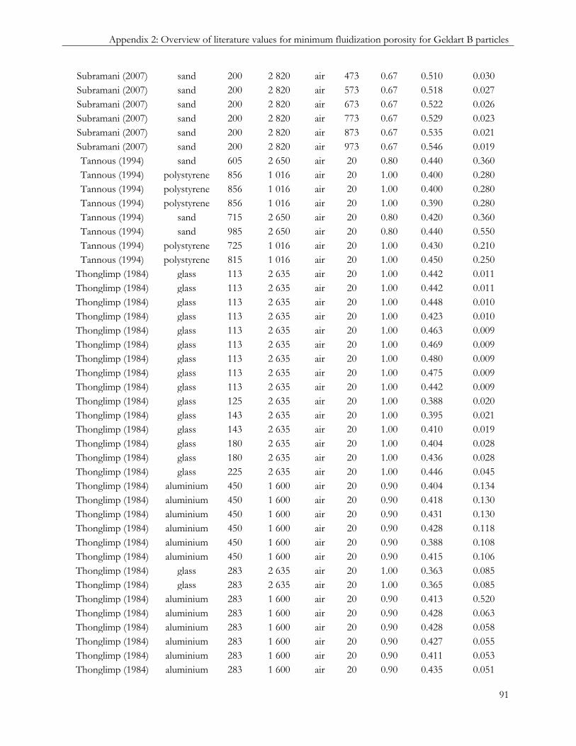
Appendix 2: Overview of literature values for minimum fluidization porosity for Geldart B particles
91
Subramani (2007) sand 200 2 820 air 473 0.67 0.510 0.030
Subramani (2007) sand 200 2 820 air 573 0.67 0.518 0.027
Subramani (2007) sand 200 2 820 air 673 0.67 0.522 0.026
Subramani (2007) sand 200 2 820 air 773 0.67 0.529 0.023
Subramani (2007) sand 200 2 820 air 873 0.67 0.535 0.021
Subramani (2007) sand 200 2 820 air 973 0.67 0.546 0.019
Tannous (1994) sand 605 2 650 air 20 0.80 0.440 0.360
Tannous (1994) polystyrene 856 1 016 air 20 1.00 0.400 0.280
Tannous (1994) polystyrene 856 1 016 air 20 1.00 0.400 0.280
Tannous (1994) polystyrene 856 1 016 air 20 1.00 0.390 0.280
Tannous (1994) sand 715 2 650 air 20 0.80 0.420 0.360
Tannous (1994) sand 985 2 650 air 20 0.80 0.440 0.550
Tannous (1994) polystyrene 725 1 016 air 20 1.00 0.430 0.210
Tannous (1994) polystyrene 815 1 016 air 20 1.00 0.450 0.250
Thonglimp (1984) glass 113 2 635 air 20 1.00 0.442 0.011
Thonglimp (1984) glass 113 2 635 air 20 1.00 0.442 0.011
Thonglimp (1984) glass 113 2 635 air 20 1.00 0.448 0.010
Thonglimp (1984) glass 113 2 635 air 20 1.00 0.423 0.010
Thonglimp (1984) glass 113 2 635 air 20 1.00 0.463 0.009
Thonglimp (1984) glass 113 2 635 air 20 1.00 0.469 0.009
Thonglimp (1984) glass 113 2 635 air 20 1.00 0.480 0.009
Thonglimp (1984) glass 113 2 635 air 20 1.00 0.475 0.009
Thonglimp (1984) glass 113 2 635 air 20 1.00 0.442 0.009
Thonglimp (1984) glass 125 2 635 air 20 1.00 0.388 0.020
Thonglimp (1984) glass 143 2 635 air 20 1.00 0.395 0.021
Thonglimp (1984) glass 143 2 635 air 20 1.00 0.410 0.019
Thonglimp (1984) glass 180 2 635 air 20 1.00 0.404 0.028
Thonglimp (1984) glass 180 2 635 air 20 1.00 0.436 0.028
Thonglimp (1984) glass 225 2 635 air 20 1.00 0.446 0.045
Thonglimp (1984) aluminium 450 1 600 air 20 0.90 0.404 0.134
Thonglimp (1984) aluminium 450 1 600 air 20 0.90 0.418 0.130
Thonglimp (1984) aluminium 450 1 600 air 20 0.90 0.431 0.130
Thonglimp (1984) aluminium 450 1 600 air 20 0.90 0.428 0.118
Thonglimp (1984) aluminium 450 1 600 air 20 0.90 0.388 0.108
Thonglimp (1984) aluminium 450 1 600 air 20 0.90 0.415 0.106
Thonglimp (1984) glass 283 2 635 air 20 1.00 0.363 0.085
Thonglimp (1984) glass 283 2 635 air 20 1.00 0.365 0.085
Thonglimp (1984) aluminium 283 1 600 air 20 0.90 0.413 0.520
Thonglimp (1984) aluminium 283 1 600 air 20 0.90 0.428 0.063
Thonglimp (1984) aluminium 283 1 600 air 20 0.90 0.428 0.058
Thonglimp (1984) aluminium 283 1 600 air 20 0.90 0.427 0.055
Thonglimp (1984) aluminium 283 1 600 air 20 0.90 0.411 0.053
Thonglimp (1984) aluminium 283 1 600 air 20 0.90 0.435 0.051
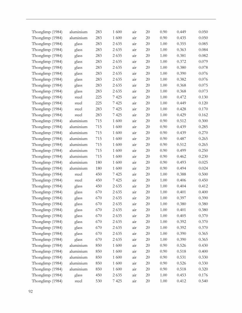
92
Thonglimp (1984) aluminium 283 1 600 air 20 0.90 0.449 0.050
Thonglimp (1984) aluminium 283 1 600 air 20 0.90 0.435 0.050
Thonglimp (1984) glass 283 2 635 air 20 1.00 0.355 0.085
Thonglimp (1984) glass 283 2 635 air 20 1.00 0.363 0.084
Thonglimp (1984) glass 283 2 635 air 20 1.00 0.381 0.082
Thonglimp (1984) glass 283 2 635 air 20 1.00 0.372 0.079
Thonglimp (1984) glass 283 2 635 air 20 1.00 0.380 0.078
Thonglimp (1984) glass 283 2 635 air 20 1.00 0.390 0.076
Thonglimp (1984) glass 283 2 635 air 20 1.00 0.382 0.076
Thonglimp (1984) glass 283 2 635 air 20 1.00 0.368 0.075
Thonglimp (1984) glass 283 2 635 air 20 1.00 0.368 0.073
Thonglimp (1984) steel 225 7 425 air 20 1.00 0.472 0.130
Thonglimp (1984) steel 225 7 425 air 20 1.00 0.449 0.120
Thonglimp (1984) steel 283 7 425 air 20 1.00 0.428 0.170
Thonglimp (1984) steel 283 7 425 air 20 1.00 0.429 0.162
Thonglimp (1984) aluminium 715 1 600 air 20 0.90 0.512 0.300
Thonglimp (1984) aluminium 715 1 600 air 20 0.90 0.439 0.285
Thonglimp (1984) aluminium 715 1 600 air 20 0.90 0.439 0.270
Thonglimp (1984) aluminium 715 1 600 air 20 0.90 0.487 0.265
Thonglimp (1984) aluminium 715 1 600 air 20 0.90 0.512 0.265
Thonglimp (1984) aluminium 715 1 600 air 20 0.90 0.499 0.250
Thonglimp (1984) aluminium 715 1 600 air 20 0.90 0.462 0.230
Thonglimp (1984) aluminium 180 1 600 air 20 0.90 0.493 0.025
Thonglimp (1984) aluminium 180 1 600 air 20 0.90 0.494 0.024
Thonglimp (1984) steel 450 7 425 air 20 1.00 0.388 0.500
Thonglimp (1984) steel 450 7 425 air 20 1.00 0.406 0.450
Thonglimp (1984) glass 450 2 635 air 20 1.00 0.404 0.412
Thonglimp (1984) glass 670 2 635 air 20 1.00 0.401 0.400
Thonglimp (1984) glass 670 2 635 air 20 1.00 0.397 0.390
Thonglimp (1984) glass 670 2 635 air 20 1.00 0.380 0.380
Thonglimp (1984) glass 670 2 635 air 20 1.00 0.401 0.380
Thonglimp (1984) glass 670 2 635 air 20 1.00 0.405 0.370
Thonglimp (1984) glass 670 2 635 air 20 1.00 0.392 0.370
Thonglimp (1984) glass 670 2 635 air 20 1.00 0.392 0.370
Thonglimp (1984) glass 670 2 635 air 20 1.00 0.390 0.365
Thonglimp (1984) glass 670 2 635 air 20 1.00 0.390 0.365
Thonglimp (1984) aluminium 850 1 600 air 20 0.90 0.526 0.430
Thonglimp (1984) aluminium 850 1 600 air 20 0.90 0.518 0.400
Thonglimp (1984) aluminium 850 1 600 air 20 0.90 0.531 0.330
Thonglimp (1984) aluminium 850 1 600 air 20 0.90 0.526 0.330
Thonglimp (1984) aluminium 850 1 600 air 20 0.90 0.518 0.320
Thonglimp (1984) glass 450 2 635 air 20 1.00 0.453 0.176
Thonglimp (1984) steel 530 7 425 air 20 1.00 0.412 0.540

Appendix 2: Overview of literature values for minimum fluidization porosity for Geldart B particles
93
Thonglimp (1984) steel 530 7 425 air 20 1.00 0.408 0.540
Thonglimp (1984) glass 450 2 635 air 20 1.00 0.458 0.175
Thonglimp (1984) glass 450 2 635 air 20 1.00 0.418 0.174
Thonglimp (1984) glass 450 2 635 air 20 1.00 0.418 0.162
Thonglimp (1984) glass 450 2 635 air 20 1.00 0.404 0.156
Thonglimp (1984) glass 450 2 635 air 20 1.00 0.418 0.156
Thonglimp (1984) glass 450 2 635 air 20 1.00 0.404 0.150
Thonglimp (1984) steel 358 7 425 air 20 1.00 0.404 0.350
Thonglimp (1984) steel 358 7 425 air 20 1.00 0.420 0.350
Thonglimp (1984) steel 565 7 425 air 20 1.00 0.409 0.720
Thonglimp (1984) steel 565 7 425 air 20 1.00 0.406 0.670
Thonglimp (1984) aluminium 950 1 600 air 20 0.90 0.518 0.410
Thonglimp (1984) aluminium 950 1 600 air 20 0.90 0.521 0.410
Thonglimp (1984) aluminium 950 1 600 air 20 0.90 0.510 0.410
Thonglimp (1984) glass 900 2 635 air 20 1.00 0.390 0.600
Thonglimp (1984) glass 900 2 635 air 20 1.00 0.380 0.550
Thonglimp (1984) glass 900 2 635 air 20 1.00 0.392 0.550
Thonglimp (1984) glass 900 2 635 air 20 1.00 0.412 0.510
Thonglimp (1984) glass 900 2 635 air 20 1.00 0.382 0.500
Thonglimp (1984) glass 900 2 635 air 20 1.00 0.392 0.500
Thonglimp (1984) glass 900 2 635 air 20 1.00 0.392 0.500
Thonglimp (1984) glass 900 2 635 air 20 1.00 0.382 0.500
Thonglimp (1984) glass 900 2 635 air 20 1.00 0.363 0.420
Thonglimp (1984) steel 670 7 425 air 20 1.00 0.406 0.800
Thonglimp (1984) steel 670 7 425 air 20 1.00 0.409 0.780
Toyohara (1992) glass 154 2 500 air 20 1.00 0.412 0.082
Toyohara (1992) glass 650 2 500 air 20 1.00 0.408 0.344
Toyohara (1992) glass 775 2 500 air 20 1.00 0.429 0.417
Toyohara (1992) glass 920 2 500 air 20 1.00 0.413 0.565

94

Appendix 3: Determination of porosity at minimum fluidization
95
Appendix 3: Determination of porosity at minimum fluidization
Recently, different research groups have successfully applied a method to determine the porosity at minimum
fluidization. They determined a pressure difference over a known height in a fluidized bed at different flow
rates beyond the minimum fluidization velocity and related this pressure difference to the bed porosity. This
procedure was repeated for several ratios of u0/umf. The average bed porosity was plotted as a function of
flow rate and extrapolated to u0/umf = 1. At this point, the porosity appeared to be the porosity at minimum
fluidization.
This procedure has been carried out in the set-up as described in Appendix 1. However, this procedure has
been extended to be able to carry out at high temperature in the proposed high temperature pseudo 2D set-
up. The procedure making use of pressure transducers has been compared to a newly proposed method
based on digital image analysis (DIA). For practical reasons, the comparison has been carried out only in a
room temperature pseudo 2D fluidized bed. To be able to perform this analysis with DIA, optical access to
the fluidized bed is required. Therefore, this method will be carried out in a pseudo 2D fluidized bed in which
images can be made in order to determine the bed height. A schematic overview of this set-up is given
inFigure A.3. A high resolution camera (Dantec FlowSense EO 16M) is used to capture images of the reactor
bed. Post processing of the images is done using the software package Dynamic Studio 3.4. The bed height at
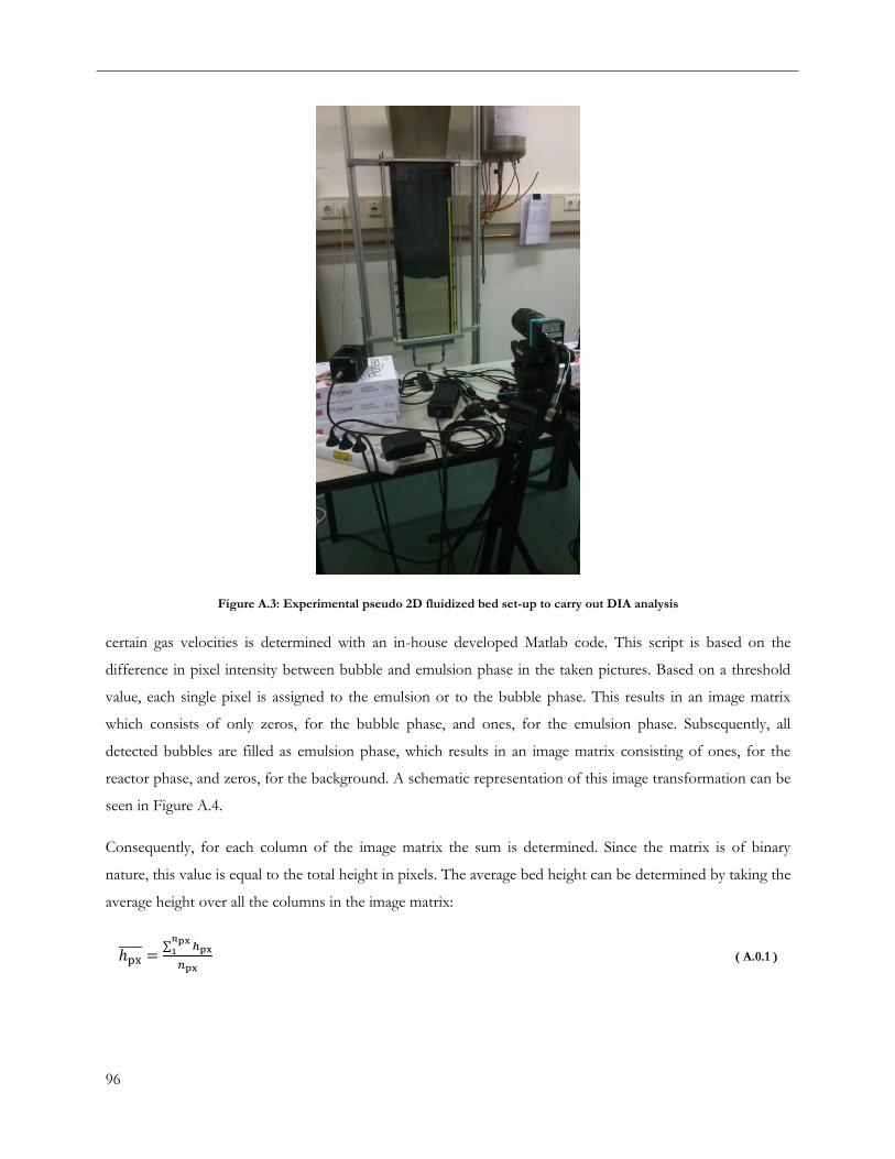
96
Figure A.3: Experimental pseudo 2D fluidized bed set-up to carry out DIA analysis
certain gas velocities is determined with an in-house developed Matlab code. This script is based on the
difference in pixel intensity between bubble and emulsion phase in the taken pictures. Based on a threshold
value, each single pixel is assigned to the emulsion or to the bubble phase. This results in an image matrix
which consists of only zeros, for the bubble phase, and ones, for the emulsion phase. Subsequently, all
detected bubbles are filled as emulsion phase, which results in an image matrix consisting of ones, for the
reactor phase, and zeros, for the background. A schematic representation of this image transformation can be
seen in Figure A.4.
Consequently, for each column of the image matrix the sum is determined. Since the matrix is of binary
nature, this value is equal to the total height in pixels. The average bed height can be determined by taking the
average height over all the columns in the image matrix:
( A.0.1 )
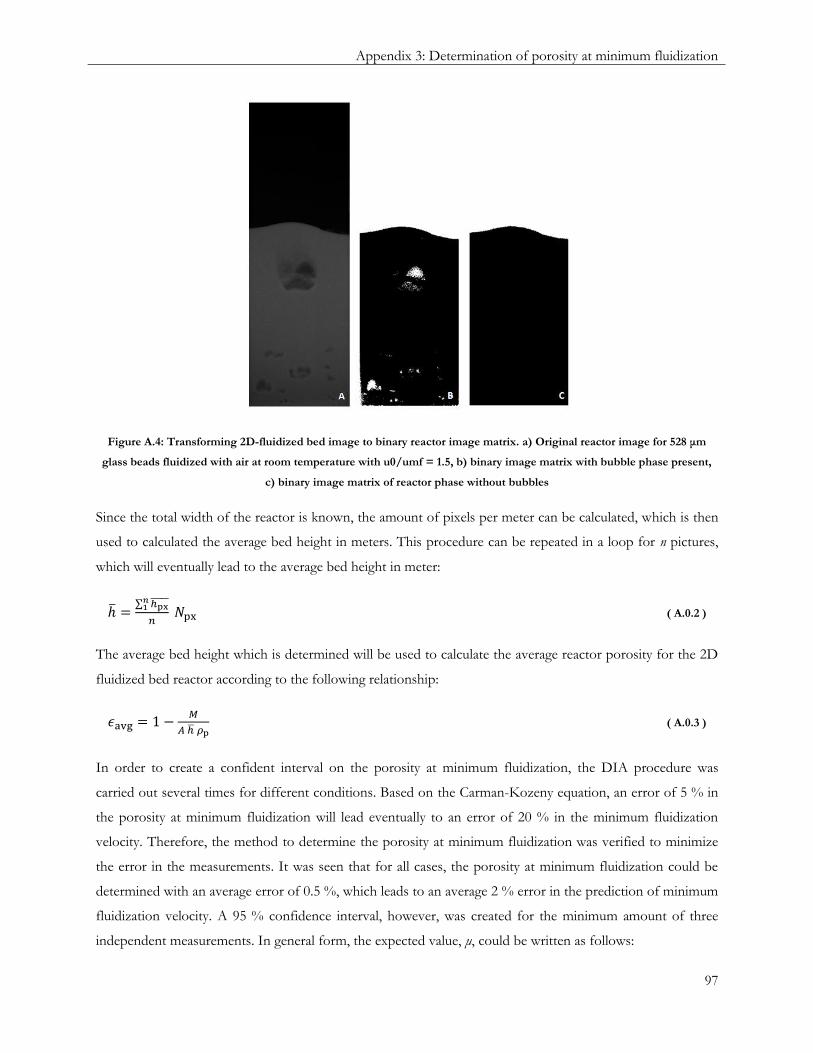
Appendix 3: Determination of porosity at minimum fluidization
97
Figure A.4: Transforming 2D-fluidized bed image to binary reactor image matrix. a) Original reactor image for 528 μm
glass beads fluidized with air at room temperature with u0/umf = 1.5, b) binary image matrix with bubble phase present,
c) binary image matrix of reactor phase without bubbles
Since the total width of the reactor is known, the amount of pixels per meter can be calculated, which is then
used to calculated the average bed height in meters. This procedure can be repeated in a loop for n pictures,
which will eventually lead to the average bed height in meter:
( A.0.2 )
The average bed height which is determined will be used to calculate the average reactor porosity for the 2D
fluidized bed reactor according to the following relationship:
( A.0.3 )
In order to create a confident interval on the porosity at minimum fluidization, the DIA procedure was
carried out several times for different conditions. Based on the Carman-Kozeny equation, an error of 5 % in
the porosity at minimum fluidization will lead eventually to an error of 20 % in the minimum fluidization
velocity. Therefore, the method to determine the porosity at minimum fluidization was verified to minimize
the error in the measurements. It was seen that for all cases, the porosity at minimum fluidization could be
determined with an average error of 0.5 %, which leads to an average 2 % error in the prediction of minimum
fluidization velocity. A 95 % confidence interval, however, was created for the minimum amount of three
independent measurements. In general form, the expected value, μ, could be written as follows:
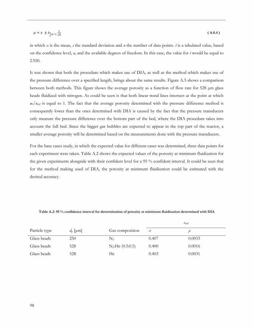
98
( A.0.4 )
in which x is the mean, s the standard deviation and n the number of data points. t is a tabulated value, based
on the confidence level, α, and the available degrees of freedom. In this case, the value for t would be equal to
2.920.
It was shown that both the procedure which makes use of DIA, as well as the method which makes use of
the pressure difference over a specified length, brings about the same results. Figure A.5 shows a comparison
between both methods. This figure shows the average porosity as a function of flow rate for 528 μm glass
beads fluidized with nitrogen. As could be seen is that both linear trend lines intersect at the point at which
u0/umf is equal to 1. The fact that the average porosity determined with the pressure difference method is
consequently lower than the ones determined with DIA is caused by the fact that the pressure transducers
only measure the pressure difference over the bottom part of the bed, where the DIA procedure takes into
account the full bed. Since the bigger gas bubbles are expected to appear in the top part of the reactor, a
smaller average porosity will be determined based on the measurements done with the pressure transducers.
For the base cases study, in which the expected value for different cases was determined, three data points for
each experiment were taken. Table A.2 shows the expected values of the porosity at minimum fluidization for
the given experiments alongside with their confident level for a 95 % confident interval. It could be seen that
for the method making used of DIA, the porosity at minimum fluidization could be estimated with the
desired accuracy.
Table A.2: 95 % confidence interval for determination of porosity at minimum fluidization determined with DIA
εmf
Particle type dp [μm] Gas composition x μ
Glass beads 250 N2 0.407 0.0033
Glass beads 528 N2:He (0.5:0.5) 0.400 0.0016
Glass beads 528 He 0.403 0.0031
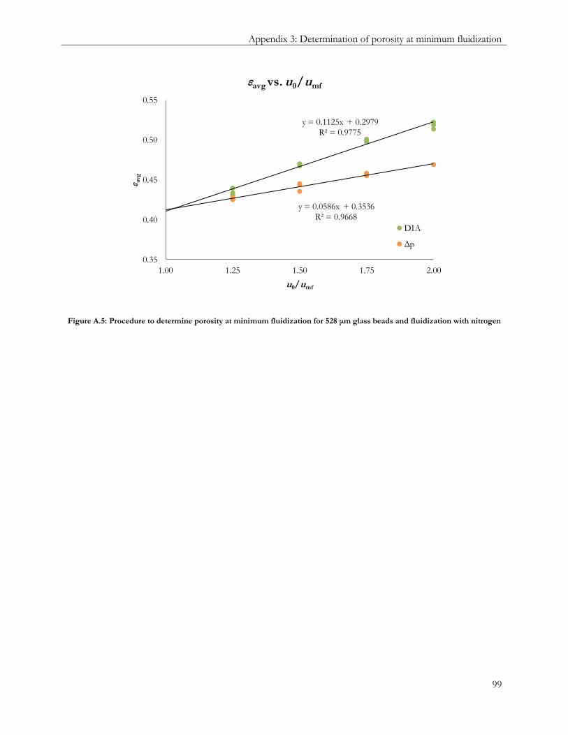
Appendix 3: Determination of porosity at minimum fluidization
99
y = 0.1125x + 0.2979
R² = 0.9775
y = 0.0586x + 0.3536
R² = 0.9668
0.35
0.40
0.45
0.50
0.55
1.00 1.25 1.50 1.75 2.00
ε avg
u0/umf
εavg vs. u0/umf
DIA
Δp
Figure A.5: Procedure to determine porosity at minimum fluidization for 528 μm glass beads and fluidization with nitrogen

100