CDE July 2013
HOW BACKWARD ARE THE OTHER BACKWARD CLASSES? CHANGING CONTOURS OF CASTE
DISADVANTAGE IN INDIA
Ashwini Deshpande Email:[email protected] Department of Economics Delhi School of Economics
Rajesh Ramachandran Email: [email protected]
Department of Microeconomics and Management Goethe University, Frankfurt
Working Paper No. 233
Centre for Development Economics Department of Economics, Delhi School of Economics
How Backward are the Other Backward Classes? Changing
Contours of Caste Disadvantage in India
Ashwini Deshpande and Rajesh Ramachandran∗
July 2013
Abstract
While there is a growing literature on the political rise of the Other Backward Classes (OBCs) in
India, where they are often seen as the new elite or the dominant castes, detailed empirical assessments of
their socio-economic condition are practically non-existent. Using individual-level data from the National
Sample Survey for 1999-2000 and 2009-2010, our paper is one of the first to undertake a comprehensive
empirical exercise, both at the national as well as the regional levels. We compare five age-cohorts,
born between the years 1926-85, for the OBCs, SC-STs and Others (everybody else) and examine the
differences in key indicators such as educational attainment, occupation and activity status, wages and
consumption expenditure through a difference-in-differences method. Our results show clear disparities in
virtually all indicators of material well-being, with Others at the top, SC-STs at the bottom and OBCs in
between. We find evidence of convergence between OBCs and Others in literacy and primary education,
but continued divergence when higher educational categories are considered. In the realm of occupation,
the younger cohorts among OBCs seem to be closing the gap vis-a-vis the Others in terms of access to
prestigious white-collar jobs. Finally comparing wage gaps for males in the labour force and estimates
of labour market discrimination, we find that while average wages of Others are higher than those for
OBCs for all age cohorts, the unexplained (or the discriminatory) component is lower for younger OBC
cohorts, compared to the older ones, and that OBCs face lower labour market discrimination compared
to SC-STs, when the average wages of both groups are compared to those of Others.
∗Corresponding author: Delhi School of Economics, University of Delhi (email: [email protected]). Second author:Departament of Microeconomics and Management, Goethe University, Frankfurt (email:[email protected]).We would like to thank Alessandro Tarozzi, Ana-Rute Cardoso and Irma Clots Figueras for their suggestions and comments.We are also grateful to the participants at the conference on “Inequality, Mobility and Sociality in Contemporary India” at YaleUniversity, April 2013 for their suggestions and useful comments. We are responsible for all remaining errors and omissions.
1
1 Introduction
The rise of the Other Backward Classes (OBCs) in the political arena since the mid-1980s has been heralded
as India’s “silent revolution” (Jafferlot, 2003). This political ascendancy has also been viewed as representing
a large enough flux in the traditional hierarchies of the caste system, such that we now have “a plethora
of assertive caste identities... [that] articulate alternative hierarchies” leading to a scenario where “there is
hardly any unanimity on ranking between jatis” Gupta (2004). Indeed, there is no doubt, especially since
the 73rd and 74th constitutional amendments in the early 1990s, that the so-called lower castes have become
an important force in Indian politics at all levels, local, state and national. Has this change in the political
arena been accompanied by a corresponding reshuffling of the traditional economic hierarchies, such as to
prevent any meaningful ranking of castes?
The nature and degree of change in the economic ranking between castes, or broad caste groups, is a
matter of empirical verification. While there is a large and growing body of work documenting the changes in
the standard of living indicators of the Scheduled Castes and Tribes (SCs and STs), as well as the economic
discrimination faced by these groups, (see Deshpande 2011, for a review of the recent research), the discussion
about the material conditions or the economic dominance of the group of castes and communities classified
as the Other Backward Classes (OBCs) in India is prompted more by beliefs, or localised case studies, rather
than by an empirical analysis of the macro evidence. Part of the reason for this lacuna is the lack of hard
data: until the 2001 census, OBCs were not counted as a separate category, while affirmative action (quotas
in India) were targeted towards OBCs at the national level since 1991, and at the state level since much
earlier. This would be the only instance of an affirmative action anywhere in the world where the targeted
beneficiaries of a national programme are not counted as a separate category in the countrys census.
Researchers have, therefore, had to rely on data from large sample surveys such as the National Sample
Survey (NSS), National Family and Health Survey (NFHS), to mention a few sources, in order to get estimates
about the material conditions of the OBCs. The use of this data has generated research which undertakes a
broader analysis of various caste groups, OBCs being one of the groups in the analysis, along with the SC-
STs and Others, the residual group of the non-SC-ST-OBC population (for instance, Deshpande 2007; Iyer
et al. 2013; Madheswaran and Attewell 2007; Zacharias and Vakulabharanam 2011, among others). Others
include the Hindu upper castes and could be considered a loose approximation for the latter, but data
constraints do not allow us to isolate the upper castes exclusively. Existing evidence suggests that OBCs lie
somewhere in between the SC-STs and the Others, but first, very little is known about their relative distance
from the two other categories and second, in order to make a meaningful intervention about the possible
links between their political ascendancy and their economic conditions, it is important to trace how their
2
relative economic position has changed vis-a-vis the other two groups over time. Here again, the economic
researcher is stymied by the lack of good longitudinal data.
The present paper is an attempt to fill this caveat in the empirical literature by focusing on an important
facet of contemporary caste inequalities, viz., the changing economic conditions of OBCs, relative to the other
two broad social/caste groups. We use data from two quinquennial rounds of the employment-unemployment
surveys (EUS) of the NSS for 1999-2000 and 2009-10 (NSS-55 and NSS-66, respectively), to examine the
multiple dimensions of material standard of living indicators, and the changes therein for the OBCs in India,
in comparison to SC-STs (for the purpose of this paper, we have pooled the two groups, because despite
considerable differences in their social situation, their economic outcomes are very similar), and the Others.
We look at five age cohorts between 25 and 74 years of age in each NSS round, and examine changes in
multiple indicators using a difference-in-differences (D-I-D) approach, comparing the three social groups to
one another over consecutive cohorts to see how the gaps on the key indicators of interest have evolved over
the 60 year period. This allows us to gauge the relative generational shifts between the major caste groups.
Our analysis focuses particularly on the OBCs, and compares how the evolution of the different OBC cohorts
(in relation to the Others) compares with the evolution of the corresponding SC-ST cohorts to the Others.
Through an analysis based on a comparison of different age cohorts, we are able to build a comprehensive
trajectory of change for each of the caste groups since independence, since the oldest cohort in our analysis
consists of individuals born between 1926 and 1935, and the youngest cohort consists of those born between
1976 and 1985. Thus, we are able to track outcomes for successive generations of individuals who reached
adulthood in the 63 years between Indian independence (in 1947) and 2010.
We start by examining the household level aggregates, such as monthly per capita expenditure (MPCE),
proportion of urban population and two landholding measures, and then move to individual indicators,
specifically, education, occupation (which focuses on occupation categories as well as the principal activity
status and changes in the Duncan dissimilarity index based on activity status) and finally wages and Blinder-
Oaxaca estimates of labour market discrimination.
Our main results can be summarized as follows. In a three-fold division of the population between SC-ST,
OBCs and Others, we see clear disparities in virtually all indicators of material well-being, with Others at the
top, SC-STs at the bottom and OBCs in between. This confirms the results from several other studies. The
average gaps between the Others and the other two social groups however remain large. MPCE, an indicator
of standard of living in developing countries, shows that the average MPCE of the OBCs and SC-ST is 51
and 65 percent of the Others, respectively. Similarly the gap between Others and OBCs for the composite
indicator of years of education remains as large as 2.21, whereas the gap between SC-ST and OBCs is 1.47
years of education. The average wages of the OBCs and SC-ST are seen to be only 42 and 55 percent of
3
the average wage of Others and the share of labour force employed in white collar prestigious jobs is just
one-fourth and half the proportion of the Others employed in white collar jobs.
Breaking down the indicator of years of education, we find evidence of convergence between OBCs and
Others in literacy and primary education, but continued divergence when higher educational categories are
considered. In the realm of occupation, the younger cohorts among OBCs seem to be closing the gap vis-
a-vis the Others in terms of access to prestigious white-collar jobs. Based on principal activity status, our
calculations of the Duncan Index reveal that OBCs are closer to the Others (less dissimilar to them) as
compared to the SC-STs (who are more dissimilar compared to the Others). For the category of regular
wage/salaried (RWS) jobs we find divergence between the Others and OBCs and SC-ST except for the very
youngest cohort. Looking at average wage gaps for males in the labour force and estimates of labour market
discrimination, we find that while average wages of Others are higher than those for OBCs for all age cohorts,
the unexplained (or the discriminatory) component is lower for younger OBC cohorts, compared to the older
ones, and that OBCs face lower labour market discrimination compared to SC-STs, when the average wages
of both groups are compared to those of Others.
2 The broad picture: household-level indicators
Table 1 presents estimates of some indicators of standard of living for three major caste groups: SC-STs
considered together, OBCs and Others, for NSS-55 and NSS-66 respectively. The indicators of interest are
MPCE, proportion of the group that is urban (percent urban) and two land holding measures: land owned
and land possessed.
D-I-D for household-level variables is calculated as:
D − I −Djk = [(Indicatorijs − Indicatoriks)− (Indicatorij(s−1)) − Indicatorik(s−1))] (1)
where j and k are the two caste groups being compared, for the ith indicator (say MPCE) between survey
rounds s and s− 1.
MPCE is shown in nominal terms: Others have the highest MPCE, followed by OBCs, and then the
SC-STs. While the MPCE for each of the groups has expectedly increased in nominal terms, the D-I-D
allows us to see the relative gains of groups. Between 1999-00 and 2009-10, we see that the MPCE gap
between OBCs and SC-STs has increased by Rs. 173 in favour of OBCs. However, for the OBCs, MPCE
has fallen behind that of the Others by Rs. 428 over the decade. Others MPCE has increased by Rs. 600
relative to SC-STs over the decade. Thus, SC-STs not only continue to have the lowest MPCE, but the
4
other two groups have gained relative to them in terms of MPCE. OBCs have gained relative to SC-STs,
but the magnitude of their falling behind Others is over 2.5 times their gain over SC-STs. Thus, on MPCE,
there is no evidence of convergence between Others, either with OBCs or with the SC-STs.
[Insert Table 1]
Urbanisation (percent of the groups population which is urban) is an indicator of structural change or of
potential integration into the modern, formal sector economy. We see a rise in urban proportions for both
OBCs and Others (at 28 and 43 percent respectively in 2009-10, but virtually no change for the SC-ST
population at around 17 percent). Again, looking at relative changes across groups using D-I-D, we find
the same pattern as that for MPCE, but the relative gain of Others over OBCs is only about 2 percentage
points. The percentage of population classified as urban for OBCs and Others increased between 3.3 and
3.55 percentage points relative to SC-STs.
The two land holding variables (land possessed and land owned) show sharp disparities in across caste
groups in both rounds, with average values for SC-STs slightly over half of the values for Others. However,
in terms of the relative change in these two variables, we see that OBCs marginally fell behind SC-STs by
0.01 hectares for land possessed, but gained over Others by close to 0.05 hectares. 1 SC-STs appear to have
gained over Others in both land owned and land possessed by 0.017 and 0.059 hectares respectively. These
changes are negligible in magnitude to have any real consequences for standard of living, and are clearly not
matched by trends in MPCE.
Overall, at the household level, we see a clear hierarchy in MPCE, such that Others are at the top,
followed by OBCs and then SC-STs. Over the decade, the gap between OBC and SC-STs has increased in
favour of the former, and Others MPCE has increased relative to both SC-STs and OBCs, but the magnitude
of gain has been larger vis-a-vis the SC-STs than OBCs.
3 Individual-level characteristics : Education
3.1 The construction of cohorts
We construct five age cohorts using the age variable in each of the NSS rounds as follows:
[Insert Table 2]
From their age, we can determine their birth year (relative to year 2000 and 2010, i.e. the end years of the
survey respectively) and thus, over the two rounds we are able to get information for six cohorts, with the
oldest being born between 1926-1935 and the youngest cohort of individuals born between 1976-1985. As
5
can be seen from the table above, matching years of birth implies that Cohort 2 in NSS-55 is Cohort 1 of
NSS-66, Cohort 3 in NSS-55 is Cohort 2 in NSS-66 and so on.
3.2 Years of education
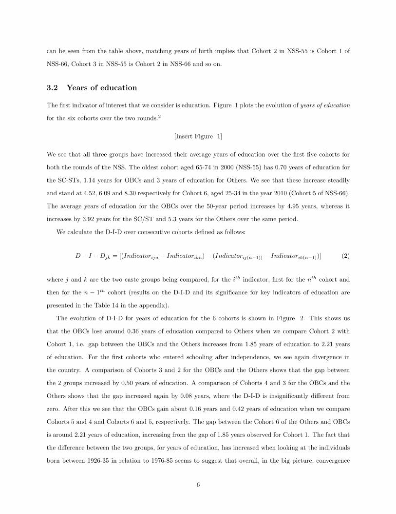
The first indicator of interest that we consider is education. Figure 1 plots the evolution of years of education
for the six cohorts over the two rounds.2
[Insert Figure 1]
We see that all three groups have increased their average years of education over the first five cohorts for
both the rounds of the NSS. The oldest cohort aged 65-74 in 2000 (NSS-55) has 0.70 years of education for
the SC-STs, 1.14 years for OBCs and 3 years of education for Others. We see that these increase steadily
and stand at 4.52, 6.09 and 8.30 respectively for Cohort 6, aged 25-34 in the year 2010 (Cohort 5 of NSS-66).
The average years of education for the OBCs over the 50-year period increases by 4.95 years, whereas it
increases by 3.92 years for the SC/ST and 5.3 years for the Others over the same period.
We calculate the D-I-D over consecutive cohorts defined as follows:
D − I −Djk = [(Indicatorijn − Indicatorikn)− (Indicatorij(n−1)) − Indicatorik(n−1))] (2)
where j and k are the two caste groups being compared, for the ith indicator, first for the nth cohort and
then for the n − 1th cohort (results on the D-I-D and its significance for key indicators of education are
presented in the Table 14 in the appendix).
The evolution of D-I-D for years of education for the 6 cohorts is shown in Figure 2. This shows us
that the OBCs lose around 0.36 years of education compared to Others when we compare Cohort 2 with
Cohort 1, i.e. gap between the OBCs and the Others increases from 1.85 years of education to 2.21 years
of education. For the first cohorts who entered schooling after independence, we see again divergence in
the country. A comparison of Cohorts 3 and 2 for the OBCs and the Others shows that the gap between
the 2 groups increased by 0.50 years of education. A comparison of Cohorts 4 and 3 for the OBCs and the
Others shows that the gap increased again by 0.08 years, where the D-I-D is insignificantly different from
zero. After this we see that the OBCs gain about 0.16 years and 0.42 years of education when we compare
Cohorts 5 and 4 and Cohorts 6 and 5, respectively. The gap between the Cohort 6 of the Others and OBCs
is around 2.21 years of education, increasing from the gap of 1.85 years observed for Cohort 1. The fact that
the difference between the two groups, for years of education, has increased when looking at the individuals
born between 1926-35 in relation to 1976-85 seems to suggest that overall, in the big picture, convergence
6
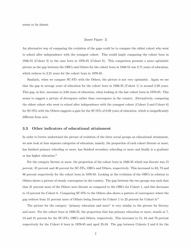
seems to be absent.
[Insert Figure 2]
An alternative way of comparing the evolution of the gaps could be to compare the oldest cohort who went
to school after independence with the youngest cohort. This would imply comparing the cohort born in
1946-55 (Cohort 3) to the ones born in 1976-85 (Cohort 6). This comparison presents a more optimistic
picture as the gap between the OBCs and Others for the cohort born in 1946-55 was 2.71 years of education,
which reduces to 2.21 years for the cohort born in 1976-85.
Similarly, when we compare SC-STs with the Others, the picture is not very optimistic. Again we see
that the gap in average years of education for the cohort born in 1926-35 (Cohort 1) is around 2.29 years.
This gap, in fact, increases to 3.68 years of education, when looking at the last cohort born in 1976-85. This
seems to suggest a picture of divergence rather than convergence in the country. Alternatively, comparing
the oldest cohort who went to school after independence with the youngest cohort (Cohort 3 and Cohort 6)
for SC-STs with the Others suggests a gain for the SC-STs of 0.08 years of education, which is insignificantly
different from zero.
3.3 Other indicators of educational attainment
In order to better understand the picture of evolution of the three social groups on educational attainment,
we now look at four separate categories of education, namely, the proportion of each cohort literate or more,
has finished primary schooling or more, has finished secondary schooling or more and finally is a graduate
or has higher education.3
For the category literate or more, the proportion of the cohort born in 1926-35 which was literate was 15
percent, 25 percent and 46 percent for SC-STs, OBCs and Others, respectively. This increased to 63, 73 and
86 percent respectively for the cohort born in 1976-85. Looking at the evolution of the OBCs in relation to
Others shows a picture of steady convergence in the country. The gap between the two groups was such that
that 21 percent more of the Others were literate as compared to the OBCs for Cohort 1, and this decreases
to 13 percent for Cohort 6. Comparing SC-STs to the Others also shows a pattern of convergence where the
gap reduces from 31 percent more of Others being literate for Cohort 1 to 23 percent for Cohort 6.4
The picture for the category “primary education and more” is very similar to the picture for literacy
and more. For the cohort born in 1926-35, the proportion that has primary education or more, stands at 7,
13 and 31 percent for the SC-STs, OBCs and Others, respectively. This increases to 51, 64 and 78 percent
respectively for the Cohort 6 born in 1976-85 and aged 25-34. The gap between Cohorts 2 and 6 for the
7
OBCs and the Others reduces from 20 percentage points to 14 percentage points. Similarly, comparing
SC-STs with Others, the gap reduces from 32 percent to 26 percent. The convergence is especially strong
for the last 3 cohorts of the OBCs, who gain 8 percentage points relative to the Others.5
The next category of education we examine is all those with “secondary education or more”. For the
cohort born in 1926-35, 2 percent of SC-STs, 3 percent of OBCs and 13 percent of Others have secondary
education or more. This increases to 19, 30 and 48 percent respectively for Cohort 6 born in 1976-85.
The evolution of the OBCs and SC- STs in relation to the Others suggests that contrary to the earlier
categories, the picture for this category of education has been one of divergence rather than convergence.
Again, comparing the gap between the two groups for Cohorts 1 and 6 suggests a picture of divergence. 10
percent more of Cohort 1 had secondary education or more for the Others as compared to the OBCs. This
gap, in fact, increases to 18 percent for Cohort 6 born in 1976-85. Similarly, for SC-STs the gap increases
from 11 percent more of Others having secondary education or more for Cohort 1 to about 29 percent for
Cohort 6.6
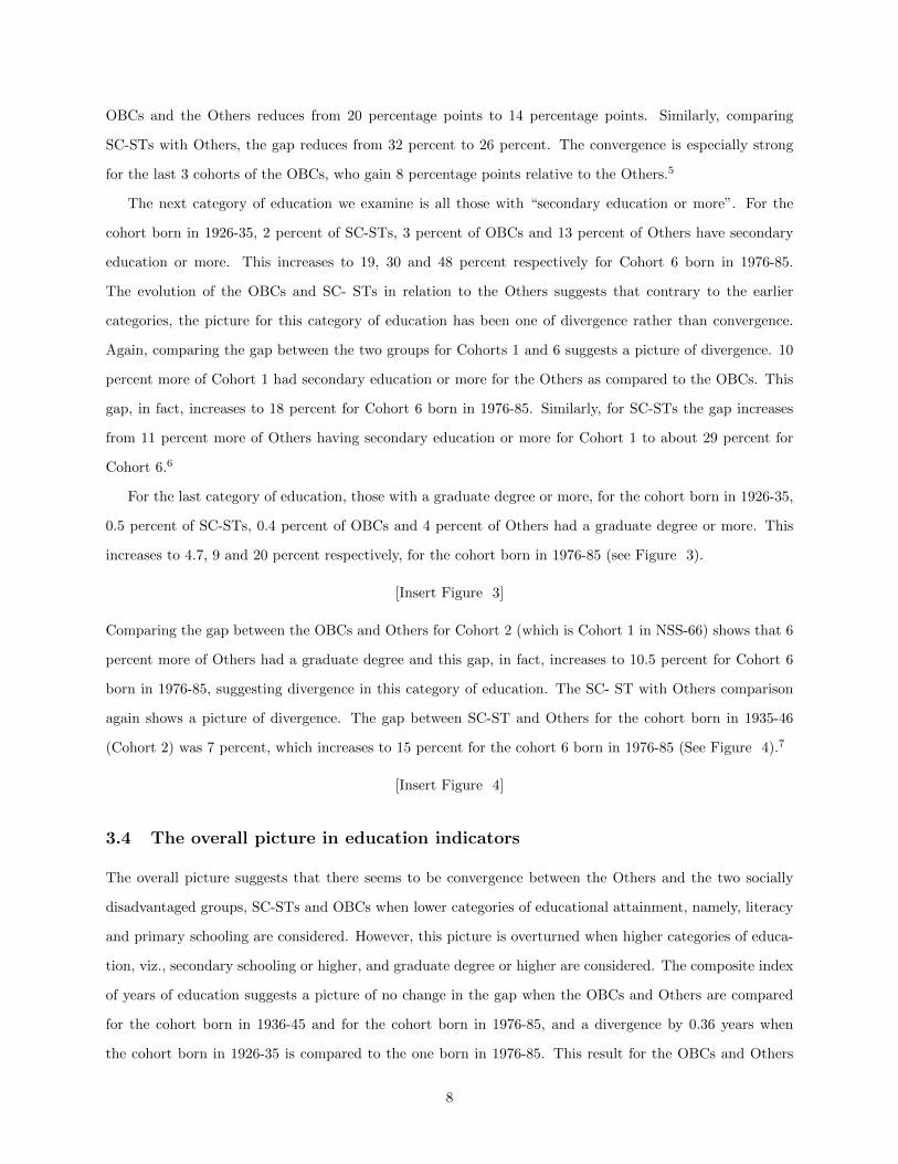
For the last category of education, those with a graduate degree or more, for the cohort born in 1926-35,
0.5 percent of SC-STs, 0.4 percent of OBCs and 4 percent of Others had a graduate degree or more. This
increases to 4.7, 9 and 20 percent respectively, for the cohort born in 1976-85 (see Figure 3).
[Insert Figure 3]
Comparing the gap between the OBCs and Others for Cohort 2 (which is Cohort 1 in NSS-66) shows that 6
percent more of Others had a graduate degree and this gap, in fact, increases to 10.5 percent for Cohort 6
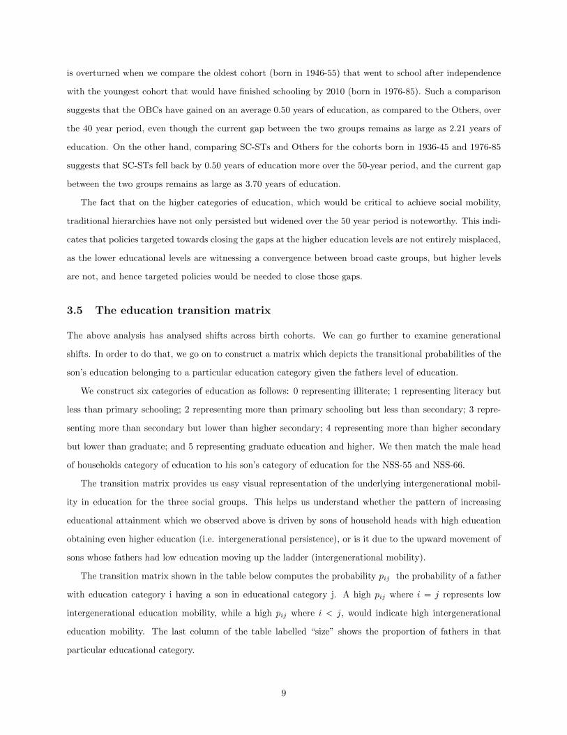
born in 1976-85, suggesting divergence in this category of education. The SC- ST with Others comparison
again shows a picture of divergence. The gap between SC-ST and Others for the cohort born in 1935-46
(Cohort 2) was 7 percent, which increases to 15 percent for the cohort 6 born in 1976-85 (See Figure 4).7
[Insert Figure 4]
3.4 The overall picture in education indicators
The overall picture suggests that there seems to be convergence between the Others and the two socially
disadvantaged groups, SC-STs and OBCs when lower categories of educational attainment, namely, literacy
and primary schooling are considered. However, this picture is overturned when higher categories of educa-
tion, viz., secondary schooling or higher, and graduate degree or higher are considered. The composite index
of years of education suggests a picture of no change in the gap when the OBCs and Others are compared
for the cohort born in 1936-45 and for the cohort born in 1976-85, and a divergence by 0.36 years when
the cohort born in 1926-35 is compared to the one born in 1976-85. This result for the OBCs and Others
8
is overturned when we compare the oldest cohort (born in 1946-55) that went to school after independence
with the youngest cohort that would have finished schooling by 2010 (born in 1976-85). Such a comparison
suggests that the OBCs have gained on an average 0.50 years of education, as compared to the Others, over
the 40 year period, even though the current gap between the two groups remains as large as 2.21 years of
education. On the other hand, comparing SC-STs and Others for the cohorts born in 1936-45 and 1976-85
suggests that SC-STs fell back by 0.50 years of education more over the 50-year period, and the current gap
between the two groups remains as large as 3.70 years of education.
The fact that on the higher categories of education, which would be critical to achieve social mobility,
traditional hierarchies have not only persisted but widened over the 50 year period is noteworthy. This indi-
cates that policies targeted towards closing the gaps at the higher education levels are not entirely misplaced,
as the lower educational levels are witnessing a convergence between broad caste groups, but higher levels
are not, and hence targeted policies would be needed to close those gaps.
3.5 The education transition matrix
The above analysis has analysed shifts across birth cohorts. We can go further to examine generational
shifts. In order to do that, we go on to construct a matrix which depicts the transitional probabilities of the
son’s education belonging to a particular education category given the fathers level of education.
We construct six categories of education as follows: 0 representing illiterate; 1 representing literacy but
less than primary schooling; 2 representing more than primary schooling but less than secondary; 3 repre-
senting more than secondary but lower than higher secondary; 4 representing more than higher secondary
but lower than graduate; and 5 representing graduate education and higher. We then match the male head
of households category of education to his son’s category of education for the NSS-55 and NSS-66.
The transition matrix provides us easy visual representation of the underlying intergenerational mobil-
ity in education for the three social groups. This helps us understand whether the pattern of increasing
educational attainment which we observed above is driven by sons of household heads with high education
obtaining even higher education (i.e. intergenerational persistence), or is it due to the upward movement of
sons whose fathers had low education moving up the ladder (intergenerational mobility).
The transition matrix shown in the table below computes the probability pij the probability of a father
with education category i having a son in educational category j. A high pij where i = j represents low
intergenerational education mobility, while a high pij where i < j, would indicate high intergenerational
education mobility. The last column of the table labelled “size” shows the proportion of fathers in that
particular educational category.
9
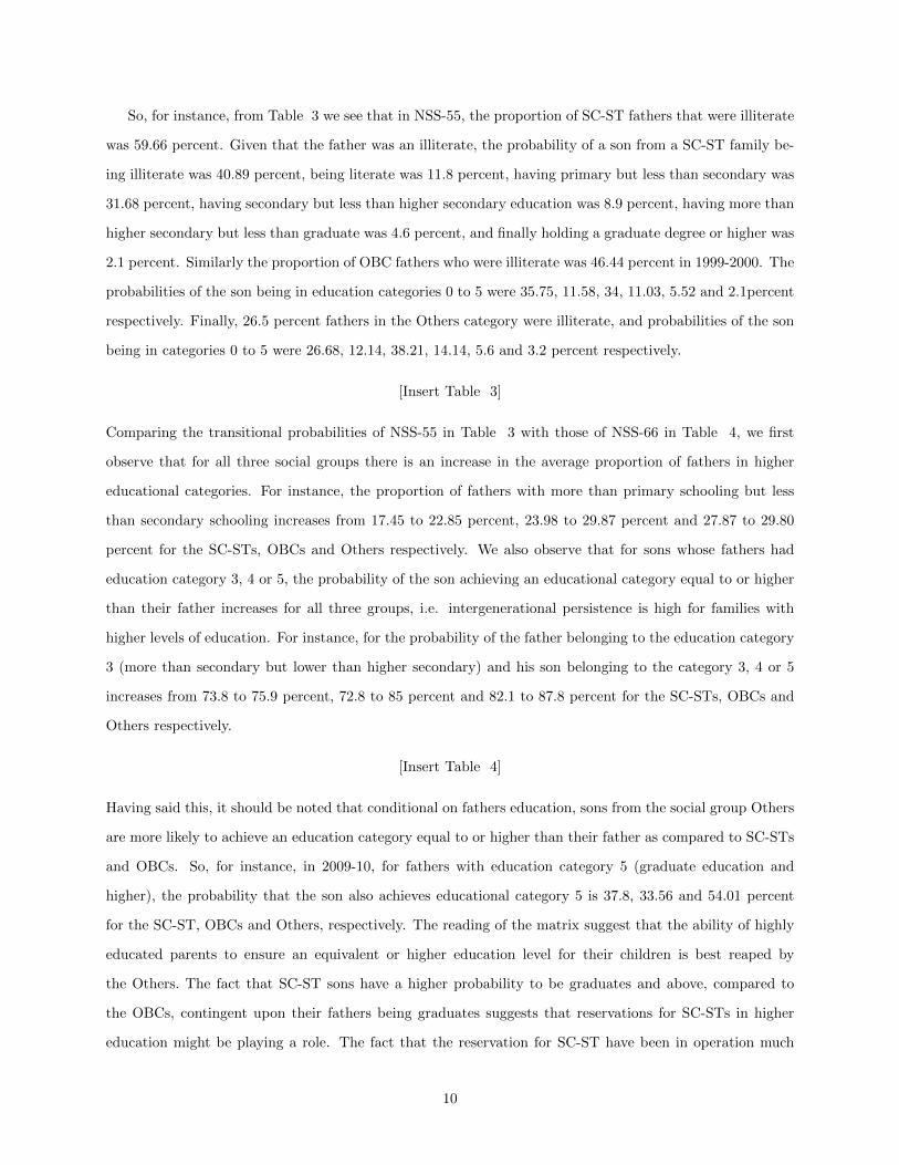
So, for instance, from Table 3 we see that in NSS-55, the proportion of SC-ST fathers that were illiterate
was 59.66 percent. Given that the father was an illiterate, the probability of a son from a SC-ST family be-
ing illiterate was 40.89 percent, being literate was 11.8 percent, having primary but less than secondary was
31.68 percent, having secondary but less than higher secondary education was 8.9 percent, having more than
higher secondary but less than graduate was 4.6 percent, and finally holding a graduate degree or higher was
2.1 percent. Similarly the proportion of OBC fathers who were illiterate was 46.44 percent in 1999-2000. The
probabilities of the son being in education categories 0 to 5 were 35.75, 11.58, 34, 11.03, 5.52 and 2.1percent
respectively. Finally, 26.5 percent fathers in the Others category were illiterate, and probabilities of the son
being in categories 0 to 5 were 26.68, 12.14, 38.21, 14.14, 5.6 and 3.2 percent respectively.
[Insert Table 3]
Comparing the transitional probabilities of NSS-55 in Table 3 with those of NSS-66 in Table 4, we first
observe that for all three social groups there is an increase in the average proportion of fathers in higher
educational categories. For instance, the proportion of fathers with more than primary schooling but less
than secondary schooling increases from 17.45 to 22.85 percent, 23.98 to 29.87 percent and 27.87 to 29.80
percent for the SC-STs, OBCs and Others respectively. We also observe that for sons whose fathers had
education category 3, 4 or 5, the probability of the son achieving an educational category equal to or higher
than their father increases for all three groups, i.e. intergenerational persistence is high for families with
higher levels of education. For instance, for the probability of the father belonging to the education category
3 (more than secondary but lower than higher secondary) and his son belonging to the category 3, 4 or 5
increases from 73.8 to 75.9 percent, 72.8 to 85 percent and 82.1 to 87.8 percent for the SC-STs, OBCs and
Others respectively.
[Insert Table 4]
Having said this, it should be noted that conditional on fathers education, sons from the social group Others
are more likely to achieve an education category equal to or higher than their father as compared to SC-STs
and OBCs. So, for instance, in 2009-10, for fathers with education category 5 (graduate education and
higher), the probability that the son also achieves educational category 5 is 37.8, 33.56 and 54.01 percent
for the SC-ST, OBCs and Others, respectively. The reading of the matrix suggest that the ability of highly
educated parents to ensure an equivalent or higher education level for their children is best reaped by
the Others. The fact that SC-ST sons have a higher probability to be graduates and above, compared to
the OBCs, contingent upon their fathers being graduates suggests that reservations for SC-STs in higher
education might be playing a role. The fact that the reservation for SC-ST have been in operation much
10
longer, than for OBCs, could be resulting in producing a greater share of graduates among SC-STs in
families where the fathers are also highly educated. It is likely that the SC-ST sons are second-generation
beneficiaries of reservations. Also, the calculated transitional probabilities suggest that the conversion of
parents endowment of education into human capital of children is highest for people from the socially
privileged, i.e. non-backward groups.
3.6 Ordered probit regressions for education categories
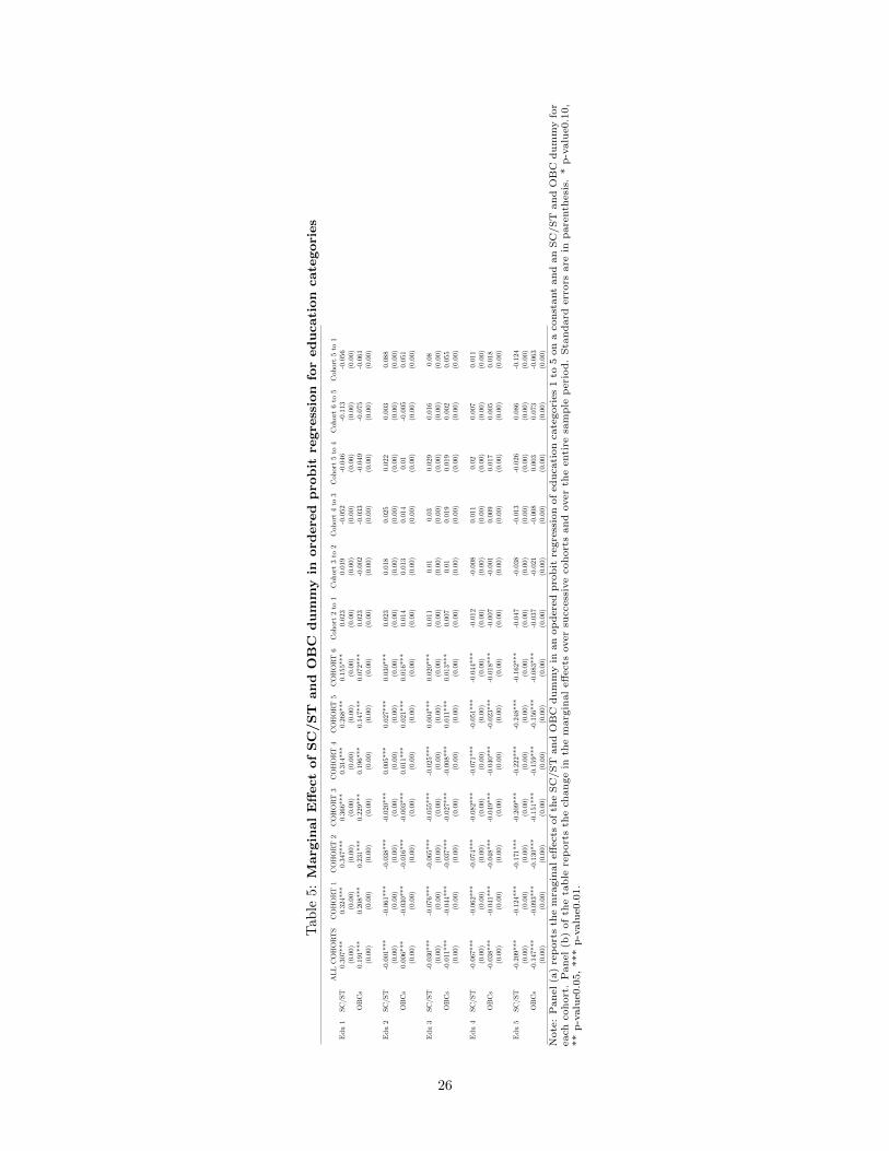
We ran an ordered probit regression to calculate the marginal effects of being in five educational categories
defined as follows: Education category 1: not literate; category 2: literate, below primary; category 3:
primary; category 4: middle; category 5: secondary and above. Table 5 shows the probabilities of being
in each of these categories for OBCs and SC-STs relative to Others. We see that all cohorts of OBCs and
SC-STs are significantly more likely to be illiterate (category 1) than Others. The marginal effects rise from
Cohort 1 to 3 and decline thereafter, such that between Cohort 1 and 5, the likelihood of OBCs being
illiterate as compared to the Others reduces from 20.6 percent to 7.2 percent. We see a similar trend for
SC-STs as well, but first, their likelihood of being illiterate relative to Others is higher than that for OBCs
and second, the decline in this probability over successive cohorts is lower than that for OBCs.
[Insert Table 5]
For higher educational categories, the trend in probabilities changes. For category 2, i.e. literate, below
primary, we see that the three youngest cohorts of OBCs show positive marginal effects compared to the
Others, indicating convergence. For the next higher category, we see that only the two youngest cohorts
of OBCs show positive marginal effects. For the last two educational categories (middle and secondary
and above), all cohorts of OBCs are less likely to be in these categories than the Others, confirming the
D-I-D result that after the middle school level, we see divergence, rather than convergence in educational
attainment.
3.7 Inequality in Years of Education
Given the differences in the educational achievement of the groups (the Others have nearly 80 percent and
37 percent more years of education than the SC-STs and OBCs respectively), we calculate some generalized
entropy measures of inequality in educational achievement, or more precisely in years of education. The
generalized entropy measures fulfil the six criteria of a good inequality measure.8
11
The measure is given by:9
GE(α) =1
α(α− 1)[1
n
n∑i=1
(yiy
)α − 1] (3)
where yi is the educational attainment of individual i and y the mean years of schooling in the population.
The parameter α in the GE class represents the weight given to distances between incomes at different parts
of the income distribution, and can take any real value. For lower values of α, GE is more sensitive to changes
in the lower tail of the distribution, and for higher values GE is more sensitive to changes that affect the
upper tail. The values of GE measures vary between 0 and ∞, with zero representing an equal distribution
and higher value representing a higher level of inequality.
The commonest values of α used are 0,1, and 2, where GE(1) is the commonly used Theil’s T Index and
GE(0) is the Theil’s L Index or the mean log deviation measure. The results are shown in Table 6.
[Insert Table 6]
We see that for all values of α in NSS-55, Others have the lowest level of inequality, followed by the OBCs,
and finally the SC-STs who have the highest level of inequality. Decomposing the inequality in educational
attainment into the between and within group components shows that the within group inequality accounts
for the substantial portion of inequality observed in the educational attainment of the three social groups.
For instance for the Theil T and L, the between component accounts for as little as 0.4 percent to 8.5 percent
of total inequality.
For NSS-66, we see that the inequality for all groups has decreased. The pattern however remains the
same, in that for all values of α, Others have the lowest level of inequality, followed by the OBCs and finally
the SC-STs have the highest level of inequality. Decomposing the total inequality into its between and
within components again shows that between-group inequality accounts for 0.2 percent and 4.1 percent of
inequality when we consider he Theil T and L index, respectively, thus both between- group and within-group
components have decreased over the decade.
4 Occupation
How does the evolution of differences in educational attainment translate into occupational differences be-
tween groups? To start this investigation, we first estimate the number of individuals in the labour force.10
We then aggregate these individuals into three categories: those with agricultural jobs, blue- collar jobs and
white-collar jobs.11
In 1999-2000, based on NSS-55, for the first cohort born in 1926-35, the proportion of those in agricultural
jobs was 78.85 for SC-ST, 74.55 for OBC and 71.85 for Others. Over successive cohorts, we see that for all
12
groups, proportion of individuals in agricultural jobs declines, to stand at 51.28, 46 and 35.46 respectively for
Cohort 4 in NSS-66 (those who are 35-44 years old in 2010).12 For blue-collar jobs, proportions for Cohort
1 in NSS-55 for the three groups are 17.78, 21.68 and 18.97 respectively, which have doubled for Cohort
4 in NSS-66 to stand at 40.4; 41.1 and 39.57 respectively. This illustrates the shift away from agriculture
towards secondary and tertiary sectors respectively. We also note that gaps between groups in agricultural
occupations are sharper than those for blue-collar jobs. The decline in proportions in agricultural jobs is
matched by an increase in proportions with blue-collar and white-collar jobs, reflecting the structural shift
in the economy, where the proportion of the population dependent on agriculture is declining over the last
several decades.
The other notable feature of the occupational division is of sharp inter-caste disparities in access to these
broad occupations. In NSS-55, SC-STs record the highest proportion in agricultural jobs consistently for all
cohorts, followed by OBCs and Others; whereas for white-collar jobs, Others record the highest proportions
for all cohorts, followed by OBCs and then SC-STs. For blue-collar jobs, the picture is mixed, in that OBCs
record the highest proportions, followed by Others and then SC-STs. A decade later, our calculations with
NSS-66 reveal a similar pattern in caste disparities, with proportions of different caste groups in blue-collar
jobs closer to each other, and with OBCs having a slight edge over the other caste groups. 13
4.1 Evolution of White-Collar Jobs
For the most prestigious white-collar jobs, caste disparities remain substantial: from 3.37 (SC-ST); 3.76
(OBC) and 9.18 (Others) percent respectively for Cohort 1 in NSS-55, the shares of the three groups stand
at 8.32; 12.93 and 24.97 respectively for Cohort 4 in NSS-66 (see Figure 5). However, we need to examine D-
I-D between cohorts across groups in order to understand the relative change between successive generations
across the three caste groups.
[Insert Figure 5]
For Cohort 1 (NSS-55), share of OBCs in white-collar jobs is 5.4 percentage points less than the Others
and that of SC-STs is 5.81 percentage points less than the Others. Looking at Cohort 5 (i.e. Cohort 4 in
NSS-66), we find that the gap between OBCs and Others has increased to 12.04 percentage points and that
between SC-STs and Others has increased to 16.65 percentage points. Thus, the share of OBCs and SC-STs
in white- collar jobs has lagged behind that of the Others, but by a greater percentage for the latter.
[Insert Figure 6]
13
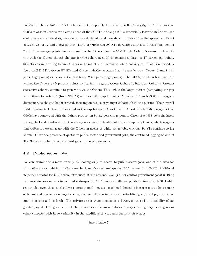
Looking at the evolution of D-I-D in share of the population in white-collar jobs (Figure 6), we see that
OBCs in absolute terms are clearly ahead of the SC-STs, although still substantially lower than Others (the
evolution and statistical significance of the calculated D-I-D are shown in Table 15 in the appendix). D-I-D
between Cohort 2 and 1 reveals that shares of OBCs and SC-STs in white collar jobs further falls behind
2 and 5 percentage points less compared to the Others. For the SC-ST only Cohort 5 seems to close the
gap with the Others though the gap for the cohort aged 35-44 remains as large as 17 percentage points.
SC-STs continue to lag behind Others in terms of their access to white collar jobs. This is reflected in
the overall D-I-D between SC-STs and Others, whether measured as the gap between Cohort 5 and 1 (-11
percentage points) or between Cohorts 5 and 2 (-6 percentage points). The OBCs, on the other hand, are
behind the Others by 5 percent points comparing the gap between Cohort 1, but after Cohort 4 through
successive cohorts, continue to gain vis-a-vis the Others. Thus, while the larger picture (comparing the gap
with Others for cohort 1 (from NSS-55) with a similar gap for cohort 5 (cohort 4 from NSS 66th), suggests
divergence, as the gap has increased, focusing on a slice of younger cohorts alters the picture. Their overall
D-I-D relative to Others, if measured as the gap between Cohort 5 and Cohort 2 in NSS-66, suggests that
OBCs have converged with the Others proportion by 3.2 percentage points. Given that NSS-66 is the latest
survey, the D-I-D evidence from this survey is a clearer indication of the contemporary trends, which suggests
that OBCs are catching up with the Others in access to white collar jobs, whereas SC-STs continue to lag
behind. Given the presence of quotas in public sector and government jobs, the continued lagging behind of
SC-STs possibly indicates continued gaps in the private sector.
4.2 Public sector jobs
We can examine this more directly by looking only at access to public sector jobs, one of the sites for
affirmative action, which in India takes the form of caste-based quotas (22.5 percent for SC-ST). Additional
27 percent quotas for OBCs were introduced at the national level (i.e. for central government jobs) in 1990;
various state governments introduced state-specific OBC quotas at different points in time after 1950. Public
sector jobs, even those at the lowest occupational tier, are considered desirable because most offer security
of tenure and several monetary benefits, such as inflation indexation, cost-of-living adjusted pay, provident
fund, pensions and so forth. The private sector wage dispersion is larger, so there is a possibility of far
greater pay at the higher end, but the private sector is an omnibus category covering very heterogeneous
establishments, with large variability in the conditions of work and payment structures.
[Insert Table 7]
14
Looking at Table 7 based on NSS-66, we see that SC-ST percentages with access to public sector jobs are
consistently higher than those for OBCs, which is at variance with the access to white collar jobs, discussed
above. We believe that the difference in the relative picture between SC-STs and OBCs reflects the longer
operation of SC-ST quotas. Others have the highest percentage of public sector jobs across cohorts. The D-I-
D reveals that OBCs are catching up, both with SC-STs and Others (the evolution and statistical significance
of the calculated D-I-D are shown in Table 15 in the appendix). This is most strikingly true for cohort 3 of
NSS-66, born between 1956-1965, individuals who would have been between 35 and 25 years old in 1990 and
hence eligible to take advantage of the new quotas. This catch-up continues onwards to cohort 4. We see
a similar convergence between SC-ST and Others, which is in contrast to the picture of divergence between
SC-ST and Others in access to white-collar jobs.
Within the public sector, white and blue-collar jobs present different scenarios. The result of quotas can
be clearly seen here. Take a representative example. 6.51 percent SC-ST, 13 percent OBCs and 26.29 percent
of Cohort 3 of NSS-66 (Cohort 4 of the six cohorts) are in white-collar jobs. But of these, 36 percent of (the
6.51) SC-ST, 21.2 percent OBCs and 24.08 percent Others are in the public sector. This reveals that there
are gaps between caste groups even within the public sector but a much higher proportion of SC-STs owes
their access to white-collar jobs to the public sector. If there had been no quotas, the SC-ST access to white
collar jobs would not have been as large as 6.51, which is already less than one-fourth the proportion of the
Others. The D-I-D for white collar public sector jobs reveals that OBCs are gaining vis--vis both SC-STs
and Others, whereas SC-STs are losing vis--vis the Others.
Thus, our suspicion that the lagging behind of the SC-STs in white collar jobs is a result of gaps in
the private sector is further confirmed by this picture. Of course, our data do not allow us to identify
quota beneficiaries explicitly; hence attributing the catch up to quotas is conjectural. The OBCs access to
white-collar jobs (both public and private), as well as public sector jobs (both blue and white-collar) shows
convergence with Others. A part of this convergence would be due to the operation of quotas but not all of
it, since there is convergence between OBCs and Others in both public and private sectors.
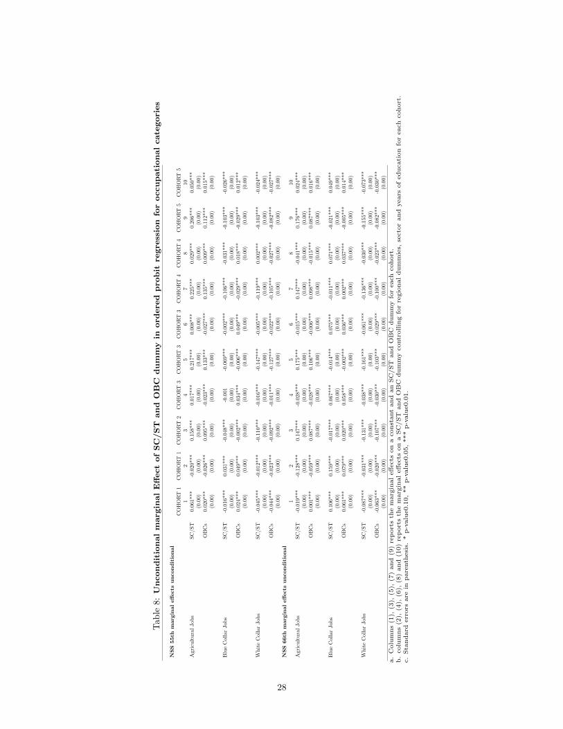
4.3 Estimating Probabilities of Job Types
We ran multinomial probit regressions separately for each cohort to estimate the probability of being in one
of the three job types (agricultural, blue-collar and white- collar) for the three caste groups. Table 8 presents
the probabilities (marginal effects) with and without controls for region, sector, and years of education for
each cohort for both rounds of NSS.
[Insert Table 8]
15
From the estimates for NSS-66, we see that SC-STs in Cohort 1 are 1.9 times less likely (without controls)
and 12.8 times less likely (with controls) be in agricultural jobs compared to Others. However, SC-STs in
Cohorts 2-5 are more likely to be in agricultural jobs compared to Others in corresponding cohorts. Similarly,
OBCs are more likely to be in agricultural jobs compared to Others in all cohorts (in regressions without
controls), but controlling for others explanatory factors, are less likely to be in agricultural jobs.
OBCs, as well as SC-STs, are less likely to be in white-collar jobs compared to Others in all cohorts,
with and without controlling for other explanatory factors. However, Table 9 shows us that the marginal
effects have by and large declined from the oldest to the youngest cohort, suggesting that the disadvantage
of younger cohorts of OBCs relative to Others appears to have decreased.
[Insert Table 9]
Comparing the marginal effects from a similar regression for NSS-55, we see that while OBCs were less likely
than Others to be in white-collar jobs also in 1999-2000, the marginal effects for the NSS-66 cohorts of OBCs
are lower, again suggesting that the relative OBC disadvantage might have reduced over the decade between
the two surveys. These regressions confirm the D-I-D trends in white-collar jobs for OBCs versus Others.
4.4 Duncans Dissimilarity Index
The NSS divides workers into a few broad categories based on their principal activity status.14 Thus, this
classification is distinct from the one used above, where we aggregated several occupations into three broad
types. Using the principal activity status, we calculate the Duncan Dissimilarity Index between groups. The
value of this index for any two groups (in our case, caste groups) gives the proportion of population that
would have to change their activity status to make the distribution of the two groups identical.
Looking at the evolution of the index across cohorts, we find that in 1999-2000, SC-STs are the most
dissimilar to the Others, with the dissimilarity rising from older to younger cohorts. Between OBCs and
Others, Cohorts 3 and 4 are more dissimilar to the Others, as compared to the other three cohorts, and
overall, all cohorts taken together, the OBCs are more similar to Others than they are to SC-STs (See Figure
7).
[Insert Figure 7]
Data from 2009-10 (see Figure 8) reveals that the dissimilarity between SC-STs and Others continues to look
the same as a decade earlier. Between OBCs and Others, too, barring Cohorts 3 and 4, where dissimilarity
between the two groups seems to have increased, the distribution is similar to what it was in 1999-2000.
Again, barring Cohort 4, the OBC distribution is closer to Others than it is to SC-STs.
16
[Insert Figure 8]
4.4.1 Understanding sources of dissimilarity
There are clear differences in the share of caste groups in the various principal status categories. Across all
cohorts, SC-ST proportions in casual wage labour are the highest, followed by OBCs and then by Others.
Mirroring this feature, we find that SC- ST proportions among employers are the lowest across all cohorts,
followed by OBCs and then by Others.
While each of these categories merits a separate analysis, in this paper we focus on two of the important
sources of dissimilarity, viz., the proportion of all workers that are regular wage/ salaried (RWS) employees
and those doing casual labour. Proportion in RWS jobs is a good indicator of involvement in the formal sec-
tor; these jobs are coveted also because of the benefits they confer to the worker, which are typically missing
from informal sector or casual jobs (some possible benefits could be inflation-linked indexation, pensions,
gratuity, illness cover, group insurance, provident fund and so forth). As Banerjee and Duflo (2011) suggest,
job security and regular wages seems to be one of the important aspirations of the poor in India. Thus, the
small proportions of SC- STs and OBCs in RWS jobs suggests that this is an important facet of occupational
disparity across caste groups.
We see that across all groups, the proportions engaged in RWS jobs have been rising, indicating the
greater formalization of jobs. As Figure 9 shows, for the Others, there is sharp rise in the proportion in
RWS jobs from Cohort 1 to Cohort 4, but the rise is not sustained in the next two cohorts. OBCs and
SC-STs too show a much sharper rise from Cohort 1 to Cohort 4, than for the latter two cohorts.
[Insert Figure 9]
What is interesting is that the D-I-D in the share of salaried employees across cohorts between groups shows
slightly different patterns between NSS-55 and NSS-66. In NSS 55 Cohort 4 and 5 of the OBCs and SC-ST
gain relative to the Others. In NSS 66 only Cohort 5 of the OBCs and SC-ST gain relative to the Others.15
Given that NSS-66 is the later survey, we can take the results from this survey as indicating the latest trends.
The share of RWS employees by cohort and their evolution of the D-I-D are shown in Figure 10 and 11,
respectively.
[Insert Figure 10]
Thus, between Cohort 2 and Cohort 1, OBCs fall 9.71 percentage points behind the Others. This gap
consistently increases and finally between Cohort 5 and 4, OBCs gain 3.28 percentage points relative to
17
Others. The SC-ST versus Others D-I-D shows the same trend, except that the final cohort gains only 0.62
percentage points relative to the Others. Over the entire sample period we see that for the OBCs the gap
increases from -0.97 percentage points for Cohort 1 to 8.9 percentage points for cohort 5 (born 1966-75).
Similarly for the SC-ST the gap increases from 1.5 percentage points for cohort 1 to 14 percentage points
for the cohort born in 1966-75. So over the 50 year period there seems to have been divergence in terms of
share of RWS between the Others and OBCs and SC-ST.
[Insert Figure 11]
Given the divergence except for the very youngest cohorts in the activity status of RWS, looking at NSS-66
we explore whether the trends in casual labour mirror those of RWS i.e. whether Others have decreased
their share of labour force in casual labour relative to the SC-ST and OBCs.
[Insert Figure 12]
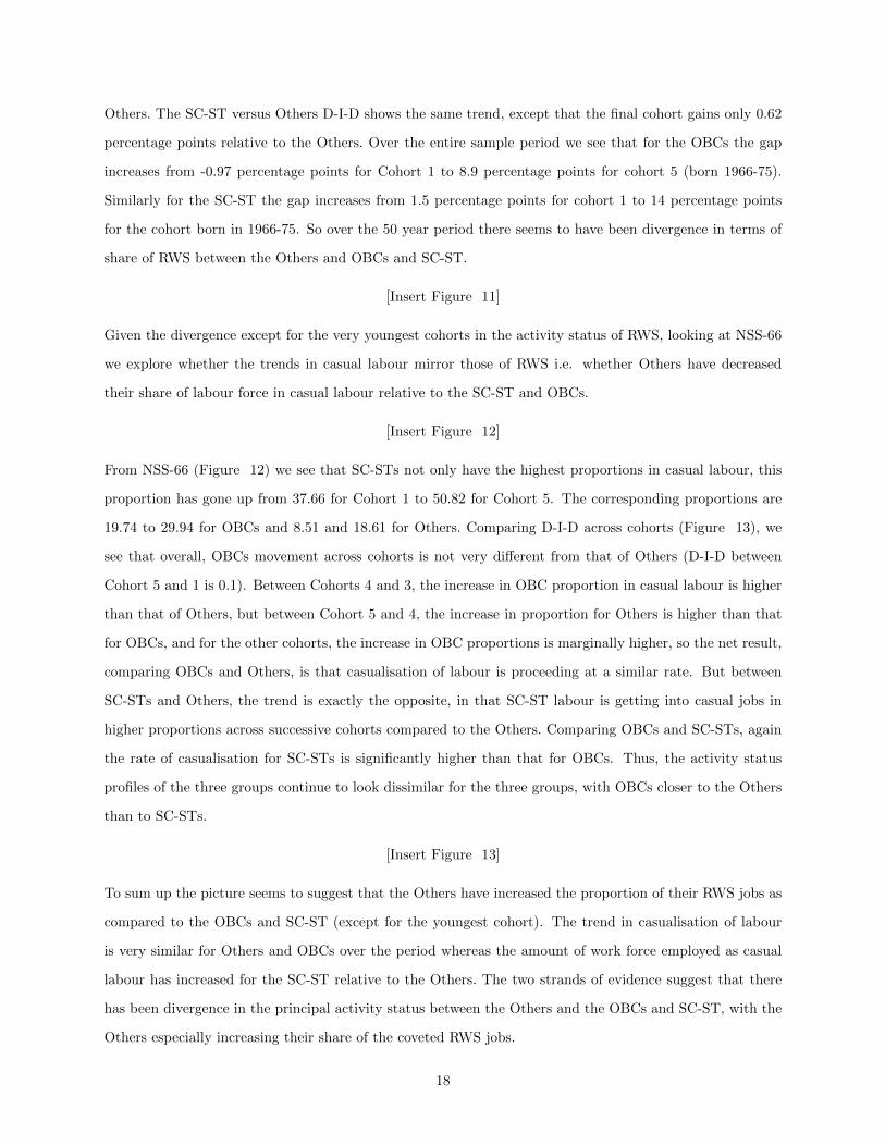
From NSS-66 (Figure 12) we see that SC-STs not only have the highest proportions in casual labour, this
proportion has gone up from 37.66 for Cohort 1 to 50.82 for Cohort 5. The corresponding proportions are
19.74 to 29.94 for OBCs and 8.51 and 18.61 for Others. Comparing D-I-D across cohorts (Figure 13), we
see that overall, OBCs movement across cohorts is not very different from that of Others (D-I-D between
Cohort 5 and 1 is 0.1). Between Cohorts 4 and 3, the increase in OBC proportion in casual labour is higher
than that of Others, but between Cohort 5 and 4, the increase in proportion for Others is higher than that
for OBCs, and for the other cohorts, the increase in OBC proportions is marginally higher, so the net result,
comparing OBCs and Others, is that casualisation of labour is proceeding at a similar rate. But between
SC-STs and Others, the trend is exactly the opposite, in that SC-ST labour is getting into casual jobs in
higher proportions across successive cohorts compared to the Others. Comparing OBCs and SC-STs, again
the rate of casualisation for SC-STs is significantly higher than that for OBCs. Thus, the activity status
profiles of the three groups continue to look dissimilar for the three groups, with OBCs closer to the Others
than to SC-STs.
[Insert Figure 13]
To sum up the picture seems to suggest that the Others have increased the proportion of their RWS jobs as
compared to the OBCs and SC-ST (except for the youngest cohort). The trend in casualisation of labour
is very similar for Others and OBCs over the period whereas the amount of work force employed as casual
labour has increased for the SC-ST relative to the Others. The two strands of evidence suggest that there
has been divergence in the principal activity status between the Others and the OBCs and SC-ST, with the
Others especially increasing their share of the coveted RWS jobs.
18
5 Wages and labour market discrimination
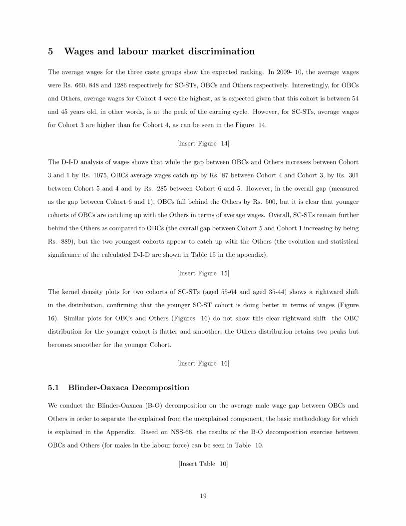
The average wages for the three caste groups show the expected ranking. In 2009- 10, the average wages
were Rs. 660, 848 and 1286 respectively for SC-STs, OBCs and Others respectively. Interestingly, for OBCs
and Others, average wages for Cohort 4 were the highest, as is expected given that this cohort is between 54
and 45 years old, in other words, is at the peak of the earning cycle. However, for SC-STs, average wages
for Cohort 3 are higher than for Cohort 4, as can be seen in the Figure 14.
[Insert Figure 14]
The D-I-D analysis of wages shows that while the gap between OBCs and Others increases between Cohort
3 and 1 by Rs. 1075, OBCs average wages catch up by Rs. 87 between Cohort 4 and Cohort 3, by Rs. 301
between Cohort 5 and 4 and by Rs. 285 between Cohort 6 and 5. However, in the overall gap (measured
as the gap between Cohort 6 and 1), OBCs fall behind the Others by Rs. 500, but it is clear that younger
cohorts of OBCs are catching up with the Others in terms of average wages. Overall, SC-STs remain further
behind the Others as compared to OBCs (the overall gap between Cohort 5 and Cohort 1 increasing by being
Rs. 889), but the two youngest cohorts appear to catch up with the Others (the evolution and statistical
significance of the calculated D-I-D are shown in Table 15 in the appendix).
[Insert Figure 15]
The kernel density plots for two cohorts of SC-STs (aged 55-64 and aged 35-44) shows a rightward shift
in the distribution, confirming that the younger SC-ST cohort is doing better in terms of wages (Figure
16). Similar plots for OBCs and Others (Figures 16) do not show this clear rightward shift the OBC
distribution for the younger cohort is flatter and smoother; the Others distribution retains two peaks but
becomes smoother for the younger Cohort.
[Insert Figure 16]
5.1 Blinder-Oaxaca Decomposition
We conduct the Blinder-Oaxaca (B-O) decomposition on the average male wage gap between OBCs and
Others in order to separate the explained from the unexplained component, the basic methodology for which
is explained in the Appendix. Based on NSS-66, the results of the B-O decomposition exercise between
OBCs and Others (for males in the labour force) can be seen in Table 10.
[Insert Table 10]
19
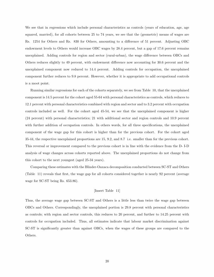
We see that in regressions which include personal characteristics as controls (years of education, age, age
squared, married), for all cohorts between 25 to 74 years, we see that the (geometric) means of wages are
Rs. 1254 for Others and Rs. 830 for Others, amounting to a difference of 51 percent. Adjusting OBC
endowment levels to Others would increase OBC wages by 28.4 percent, but a gap of 17.6 percent remains
unexplained. Adding controls for region and sector (rural-urban), the wage difference between OBCs and
Others reduces slightly to 49 percent, with endowment difference now accounting for 30.6 percent and the
unexplained component now reduced to 14.4 percent. Adding controls for occupation, the unexplained
component further reduces to 9.8 percent. However, whether it is appropriate to add occupational controls
is a moot point.
Running similar regressions for each of the cohorts separately, we see from Table 10, that the unexplained
component is 14.5 percent for the cohort aged 55-64 with personal characteristics as controls, which reduces to
12.1 percent with personal characteristics combined with region and sector and to 3.2 percent with occupation
controls included as well. For the cohort aged 45-54, we see that the unexplained component is higher
(24 percent) with personal characteristics; 21 with additional sector and region controls and 10.9 percent
with further addition of occupation controls. In others words, for all three specifications, the unexplained
component of the wage gap for this cohort is higher than for the previous cohort. For the cohort aged
35-44, the respective unexplained proportions are 15, 9.2, and 8.7 i.e. smaller than for the previous cohort.
This reversal or improvement compared to the previous cohort is in line with the evidence from the D- I-D
analysis of wage changes across cohorts reported above. The unexplained proportions do not change from
this cohort to the next youngest (aged 25-34 years).
Comparing these estimates with the Blinder-Oaxaca decomposition conducted between SC-ST and Others
(Table 11) reveals that first, the wage gap for all cohorts considered together is nearly 92 percent (average
wage for SC-ST being Rs. 653.86).
[Insert Table 11]
Thus, the average wage gap between SC-ST and Others is a little less than twice the wage gap between
OBCs and Others. Correspondingly, the unexplained portion is 29.8 percent with personal characteristics
as controls; with region and sector controls, this reduces to 20 percent, and further to 14.25 percent with
controls for occupation included. Thus, all estimates indicate that labour market discrimination against
SC-ST is significantly greater than against OBCs, when the wages of these groups are compared to the
Others.
20
6 Conclusion
The findings suggest that the gap between the Others and OBCs and SC-ST remain large for a variety of
important indicators. MPCE and wages of the OBCs and SC-ST are 51 and 65 percent and 42 and 55
percent, respectively, of the average of the Others. Their shares of labour force employed in white collar
prestigious jobs is about one fourth and half the proportion of the Others employed in white collar jobs.
On the other hand their share of labour force employed as casual labour is twice and thrice higher than the
Others for the OBCs and SC-ST, respectively. However, despite significant gaps in the above indicators,
we find substantial evidence of catch- up between OBCs and Others for the younger cohorts (especially
in literacy, primary education, access to white-collar jobs, wages), but we find continued divergence in all
education categories after the middle school level. This picture is different from the one that emerges after a
similar analysis between SC-STs and Others, where the divergence and dissimilarity in all indicators vis-a-vis
the Others is much greater. The only exception is in the education transition matrix: we find that sons of
graduate fathers are more likely to be graduates for SC-STs than for OBCs. This could possibly be the result
of the longer history of educational quotas for SC-STs in institutes of higher education as compared to that
for OBCs. Younger cohorts of OBCs are closer to the Others than to SC-STs in all indicators, whereas the
older cohorts were closer to the SC-STs in several key indicators. What precise factors have contributed to
the OBC catch-up needs to be investigated, and we hope to be able to address this in our on going research.
References
[1] Banerji, A. and Duflo, E. (2011), Poor Economics: A Radical Rethinking of the Way to Fight Global
Poverty, Public Affairs. New York, USA
[2] Deshpande, A. (2007), “Overlapping Identities under Liberalisation: Gender and Caste in India,” Eco-
nomic Development and Cultural Change, 55(4): 735-760.
[3] Deshpande, A. (2011), The Grammar of Caste: Economic Discrimination in Contemporary India,
Oxford University Press, New Delhi.
[4] Gupta, D. (2004), (editor) ‘Caste in Question: Identity or Hierarchy?” Contributions to Indian Sociol-
ogy: Occasional Studies 12, Sage Publications, New Delhi.
[5] Hnatkovska, V. and Lahiri, A. and Paul, S. (2012), “Castes and Labor Mobility,” American Economic
Journal: Applied Economics, 4(2): 274-307
21
[6] Lakshmi, I. and Khanna,T. and Varshney, A. (2013), “Caste and Entrepreneurship in India,” Economic
and Political Weekly, XLVIII(6): 52-60
[7] Jafferlot, C. (2003), Indias Silent Revolution: The Rise of Low Castes in North Indian Politics, Perma-
nent Black, New Delhi.
[8] Jann, B. (2008), “The Blinder-Oaxaca decomposition for linear regression models,” The Stata Journal
8(4): 453-479.
[9] Vakulabharanam, V. and Zacharias, A. (2011), “Caste Stratification and Wealth Inequality in India,”
World Development, 39(10): 1820-1833.
22
Notes
11 acre=0.4047 hectares. Land possessed is defined as land (owned+leased-in+neither owned nor leased- in)- land leased
out.
2The NSS does not have information on years of education. We use the method followed in Hnatkovska et al. (2012) for
converting information on educational attainment to years of education. Thus, those with formal schooling were assigned 0
years of education; those with schooling below primary were assigned 2 years; those with primary completed 5 years; those with
middle school completed 7 years; those with secondary completed 10 years; those with higher secondary 12 years; those with
graduate degrees in technology, engineering, medicine and agriculture 16 years and those with graduate degrees in all other
subjects were assigned 15 years.
3The detailed tables and charts for all the educational categories are available with the authors upon request. In the interest
of space, we are only presenting the figures on years of education and for the educational category “graduate and above”.
4If we consider the Cohort aged 15-24, i.e. those who should have achieved literacy by the time the survey was done, the
gaps further reduce, and the Others have a lead of 7 percent and 13 percent over the OBCs and SC/ST, respectively.
5If we consider the Cohort aged 15-24, i.e. those who should have finished primary schooling by the time the survey was
done, the gaps further reduce, and the Others have a lead of 9 percent and 16 percent over the OBCs and SC-STs, respectively.
6Here even if we compare the oldest cohort who went to school after independence (cohort 3), with the youngest cohort who
would have finished schooling by 2010 (cohort 6) makes the D-I-D for the OBCs compared to the Others marginally positive
(1 percent) but insignificant, whereas for the SC-STs and Others, it remains negative and significant (gap of 5 percent).
7Comparing the oldest cohort that went to school after independence (cohort 3) with the youngest cohort that would have
finished schooling by 2010 (cohort 6), the D-I-D for the OBCs and SC-STs compared to the Others remains negative and
significant.
8These are namely mean mean independence, population size independence, symmetry, Pigou-Dalton Transfer sensitivity,
decomposability and statistical testability.
9Note that the above is true for all values of α 6= 0, 1.GE(1) = 1n
∑ni=1[ yi
yln( yi
y)] and GE(0) = 1
n
∑ni=1[ln( y
yi)]
10In the NSS EUS, these are all individuals with principal activity status codes between 11 and 81.
11We use NCO-68 codes for this classification. Following Hnatkovska et al. (2012), all those with NCO codes between 600
and 699 are classified as being in agricultural jobs; those between 400 and 599 or between 700 and 999 as being in blue-collar
jobs; and those between 0 and 399 are classified as having white-collar jobs.
12When we trace the evolution of occupations, we focus on Cohort 1 of NSS-55 (the oldest cohort) and compare that with
Cohort 4 of NSS-66, which is the second youngest cohort in our data set. The youngest group is cohort 5 in NSS- 66, but these
are individuals between 25-34 years of age and might be still be in a state of transition in terms of their occupational choices.
Those aged 35-44 years would be more likely settled in their choices.
13The appendix shows the table showing the distribution of the labour force across the 3 occupations for the 3 social groups.
14 The principal activity status has the following categories: own-account worker, employer, helper in household enterprise,
regular wage/ salaried employment; casual wage labour in public works; casual wage labour in other types of work.
15The graphs for the NSS 55th are provided in the appendix.
23
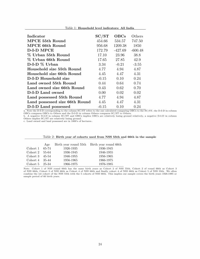
Table 1: Household level indicators: All India
Indicator SC/ST OBCs OthersMPCE 55th Round 454.66 534.57 747.50MPCE 66th Round 956.68 1209.38 1850D-I-D MPCE 172.79 -427.69 -600.48% Urban 55th Round 17.10 23.96 38.8% Urban 66th Round 17.65 27.85 42.9D-I-D % Urban 3.34 -0.21 -3.55Household size 55th Round 4.77 4.94 4.87Household size 66th Round 4.45 4.47 4.31D-I-D Household size -0.15 0.10 0.24Land owned 55th Round 0.44 0.64 0.74Land owned size 66th Round 0.43 0.62 0.70D-I-D Land owned 0.00 0.02 0.02Land possessed 55th Round 4.77 4.94 4.87Land possessed size 66th Round 4.45 4.47 4.31D-I-D Land possessed -0.15 0.10 0.24
a. Note the D-I-D corresponding to the column SC/ST refers to the one calculated comparing OBCs to the SC/ST, the D-I-D in columnOBCs compares OBCs to Others and the D-I-D in column Others compares SC/ST to Others.b. A negative D-I-D in column SC/ST and OBCs implies OBCs are relatively losing ground relatively, a negative D-I-D in columnOthers implies SC/ST are relatively losing ground.c. Land owned and land possessed are in 1000’s of hectares..
Table 2: Birth year of cohorts used from NSS 55th and 66th in the sample
Age Birth year round 55th Birth year round 66thCohort 1 65-74 1926-1935 1936-1945Cohort 2 55-64 1936-1945 1946-1955Cohort 3 45-54 1946-1955 1956-1965Cohort 4 35-44 1956-1965 1966-1975Cohort 5 25-34 1966-1975 1976-1985
Note: Cohort 1 of NSS round 66th has the same birth years as Cohort 2 of NSS 55th, Cohort 2 of round 66th as Cohort 3of NSS 66th, Cohort 3 of NSS 66th as Cohort 4 of NSS 66th and finally cohort 4 of NSS 66th as Cohort 5 of NSS 55th. We oftencombine the 1st cohort of the NSS 55th with the 5 cohorts of NSS 66th. This implies our sample covers the birth years 1926-1985 orsample period of 60 birth years.
24
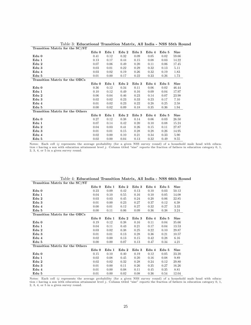
Table 3: Educational Transition Matrix, All India - NSS 55th RoundTransition Matrix for the SC/ST
Edu 0 Edu 1 Edu 2 Edu 3 Edu 4 Edu 5 SizeEdu 0 0.41 0.12 0.32 0.09 0.05 0.02 59.66Edu 1 0.13 0.17 0.44 0.15 0.08 0.03 14.22Edu 2 0.07 0.06 0.49 0.20 0.11 0.06 17.45Edu 3 0.03 0.01 0.22 0.29 0.32 0.13 5.11Edu 4 0.03 0.02 0.19 0.26 0.32 0.19 1.83Edu 5 0.01 0.00 0.17 0.22 0.33 0.26 1.73Transition Matrix for the OBCs
Edu 0 Edu 1 Edu 2 Edu 3 Edu 4 Edu 5 SizeEdu 0 0.36 0.12 0.34 0.11 0.06 0.02 46.44Edu 1 0.10 0.12 0.49 0.16 0.09 0.04 17.97Edu 2 0.06 0.04 0.46 0.23 0.14 0.07 23.98Edu 3 0.02 0.02 0.23 0.33 0.23 0.17 7.10Edu 4 0.01 0.02 0.23 0.22 0.28 0.25 2.58Edu 5 0.00 0.02 0.09 0.18 0.35 0.36 1.94Transition Matrix for the Others
Edu 0 Edu 1 Edu 2 Edu 3 Edu 4 Edu 5 SizeEdu 0 0.27 0.12 0.38 0.14 0.06 0.03 26.50Edu 1 0.07 0.14 0.42 0.20 0.10 0.08 15.24Edu 2 0.04 0.03 0.41 0.26 0.15 0.11 27.87Edu 3 0.01 0.01 0.15 0.28 0.28 0.26 14.95Edu 4 0.02 0.00 0.10 0.21 0.34 0.33 5.90Edu 5 0.02 0.00 0.04 0.13 0.32 0.49 9.55
Notes: Each cell ij represents the average probability (for a given NSS survey round) of a household male head with educa-tion i having a son with education attainment level j. Column titled “size” reports the fraction of fathers in education category 0, 1,2, 3, 4, or 5 in a given survey round.
Table 4: Educational Transition Matrix, All India - NSS 66th RoundTransition Matrix for the SC/ST
Edu 0 Edu 1 Edu 2 Edu 3 Edu 4 Edu 5 SizeEdu 0 0.23 0.09 0.42 0.13 0.10 0.03 50.12Edu 1 0.04 0.10 0.55 0.16 0.10 0.05 14.08Edu 2 0.03 0.03 0.45 0.24 0.20 0.06 22.85Edu 3 0.01 0.00 0.23 0.27 0.37 0.12 6.38Edu 4 0.00 0.01 0.12 0.27 0.32 0.27 3.33Edu 5 0.00 0.11 0.06 0.09 0.36 0.38 3.24Transition Matrix for the OBCs
Edu 0 Edu 1 Edu 2 Edu 3 Edu 4 Edu 5 SizeEdu 0 0.19 0.12 0.38 0.16 0.11 0.04 35.66Edu 1 0.04 0.11 0.43 0.21 0.17 0.04 13.53Edu 2 0.03 0.02 0.38 0.25 0.22 0.10 29.87Edu 3 0.01 0.01 0.13 0.28 0.36 0.21 10.57Edu 4 0.02 0.00 0.13 0.15 0.42 0.28 6.16Edu 5 0.00 0.00 0.07 0.13 0.47 0.34 4.21Transition Matrix for the Others
Edu 0 Edu 1 Edu 2 Edu 3 Edu 4 Edu 5 SizeEdu 0 0.15 0.10 0.40 0.19 0.12 0.05 23.20Edu 1 0.02 0.08 0.45 0.20 0.16 0.08 9.89Edu 2 0.02 0.02 0.32 0.28 0.24 0.12 29.80Edu 3 0.01 0.00 0.11 0.26 0.35 0.27 16.26Edu 4 0.01 0.00 0.08 0.11 0.45 0.35 8.81Edu 5 0.01 0.00 0.02 0.08 0.36 0.54 12.04
Notes: Each cell ij represents the average probability (for a given NSS survey round) of a household male head with educa-tion i having a son with education attainment level j. Column titled “size” reports the fraction of fathers in education category 0, 1,2, 3, 4, or 5 in a given survey round.
25
Tab
le5:
Marg
inal
Eff
ect
of
SC
/ST
and
OB
Cdum
my
inord
ere
dpro
bit
regre
ssio
nfo
reducati
on
cate
gori
es
AL
LC
OH
OR
TS
CO
HO
RT
1C
OH
OR
T2
CO
HO
RT
3C
OH
OR
T4
CO
HO
RT
5C
OH
OR
T6
Coh
ort
2to
1C
ohor
t3
to2
Coh
ort
4to
3C
ohor
t5
to4
Coh
ort
6to
5C
ohort
5to
1E
du
1SC
/ST
0.30
7***
0.32
4***
0.3
47**
*0.
366
***
0.31
4***
0.26
8***
0.15
5***
0.02
30.
019
-0.0
52-0
.046
-0.1
13-0
.056
(0.0
0)(0
.00)
(0.0
0)(0
.00)
(0.0
0)(0
.00)
(0.0
0)(0
.00)
(0.0
0)(0
.00)
(0.0
0)(0
.00)
(0.0
0)
OB
Cs
0.19
1***
0.20
8***
0.231
***
0.22
9***
0.19
6***
0.14
7***
0.07
2***
0.02
3-0
.002
-0.0
33-0
.049
-0.0
75-0
.061
(0.0
0)(0
.00)
(0.0
0)(0
.00)
(0.0
0)(0
.00)
(0.0
0)(0
.00)
(0.0
0)(0
.00)
(0.0
0)(0
.00)
(0.0
0)
Edu
2SC
/ST
-0.0
01**
*-0
.061
***
-0.0
38*
**-0
.020
***
0.00
5***
0.02
7***
0.03
0***
0.02
30.
018
0.02
50.
022
0.00
30.0
88
(0.0
0)(0
.00)
(0.0
0)(0
.00)
(0.0
0)(0
.00)
(0.0
0)(0
.00)
(0.0
0)(0
.00)
(0.0
0)(0
.00)
(0.0
0)
OB
Cs
0.00
6***
-0.0
30**
*-0
.016*
**-0
.003
***
0.01
1***
0.02
1***
0.01
6***
0.01
40.
013
0.01
40.
01-0
.005
0.0
51
(0.0
0)(0
.00)
(0.0
0)(0
.00)
(0.0
0)(0
.00)
(0.0
0)(0
.00)
(0.0
0)(0
.00)
(0.0
0)(0
.00)
(0.0
0)
Edu
3SC
/ST
-0.0
30**
*-0
.076
***
-0.0
65*
**-0
.055
***
-0.0
25*
**0.
004*
**0.0
20**
*0.
011
0.01
0.03
0.02
90.
016
0.0
8(0
.00)
(0.0
0)(0
.00)
(0.0
0)
(0.0
0)(0
.00)
(0.0
0)(0
.00)
(0.0
0)(0
.00)
(0.0
0)(0
.00)
(0.0
0)
OB
Cs
-0.0
11**
*-0
.044
***
-0.0
37**
*-0
.027
***
-0.0
08**
*0.
011*
**0.
013*
**0.
007
0.01
0.01
90.
019
0.00
20.0
55
(0.0
0)(0
.00)
(0.0
0)(0
.00)
(0.0
0)(0
.00)
(0.0
0)(0
.00)
(0.0
0)(0
.00)
(0.0
0)(0
.00)
(0.0
0)
Edu
4SC
/ST
-0.0
67**
*-0
.062
***
-0.0
74*
**-0
.082
***
-0.0
71*
**-0
.051
***
-0.0
44**
*-0
.012
-0.0
080.
011
0.02
0.00
70.0
11
(0.0
0)(0
.00)
(0.0
0)(0
.00)
(0.0
0)(0
.00)
(0.0
0)(0
.00)
(0.0
0)(0
.00)
(0.0
0)(0
.00)
(0.0
0)
OB
Cs
-0.0
38**
*-0
.041
***
-0.0
48**
*-0
.049
***
-0.0
40**
*-0
.023
***
-0.0
18**
*-0
.007
-0.0
010.
009
0.01
70.
005
0.0
18
(0.0
0)(0
.00)
(0.0
0)(0
.00)
(0.0
0)(0
.00)
(0.0
0)(0
.00)
(0.0
0)(0
.00)
(0.0
0)(0
.00)
(0.0
0)
Edu
5SC
/ST
-0.2
09**
*-0
.124
***
-0.1
71*
**-0
.209
***
-0.2
22*
**-0
.248
***
-0.1
62**
*-0
.047
-0.0
38-0
.013
-0.0
260.
086
-0.1
24
(0.0
0)(0
.00)
(0.0
0)(0
.00)
(0.0
0)(0
.00)
(0.0
0)(0
.00)
(0.0
0)(0
.00)
(0.0
0)(0
.00)
(0.0
0)
OB
Cs
-0.1
47**
*-0
.093
***
-0.1
30**
*-0
.151
***
-0.1
59**
*-0
.156
***
-0.0
83**
*-0
.037
-0.0
21-0
.008
0.00
30.
073
-0.0
63
(0.0
0)(0
.00)
(0.0
0)(0
.00)
(0.0
0)(0
.00)
(0.0
0)(0
.00)
(0.0
0)(0
.00)
(0.0
0)(0
.00)
(0.0
0)
Note
:P
anel(a
)re
port
sth
em
ragin
aleff
ects
of
the
SC
/ST
and
OB
Cdum
my
inan
op
dere
dpro
bit
regre
ssio
nof
educati
on
cate
gori
es
1to
5on
aconst
ant
and
an
SC
/ST
and
OB
Cdum
my
for
each
cohort
.P
anel
(b)
of
the
table
rep
ort
sth
ech
ange
inth
em
arg
inal
eff
ects
over
success
ive
cohort
sand
over
the
enti
resa
mple
peri
od.
Sta
ndard
err
ors
are
inpare
nth
esi
s.*
p-v
alu
e0.1
0,
**
p-v
alu
e0.0
5,
***
p-v
alu
e0.0
1.
26
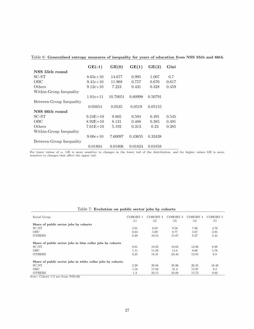
Table 6: Generalized entropy measures of inequality for years of education from NSS 55th and 66th
GE(-1) GE(0) GE(1) GE(2) GiniNSS 55th roundSC-ST 8.65e+10 14.677 0.995 1.007 0.7OBC 9.41e+10 11.968 0.757 0.676 0.617Others 9.12e+10 7.223 0.431 0.328 0.459Within-Group Inequality
1.01e+11 10.70051 0.60998 0.50791Between-Group Inequality
0.05654 0.0535 0.0519 0.05155NSS 66th roundSC-ST 9.24E+10 9.805 0.594 0.491 0.545OBC 8.92E+10 8.131 0.488 0.385 0.491Others 7.61E+10 5.192 0.313 0.23 0.385Within-Group Inequality
9.00e+10 7.60097 0.43655 0.33438Between-Group Inequality
0.01804 0.01806 0.01824 0.01858
For lower values of α, GE is more sensitive to changes in the lower tail of the distribution, and for higher values GE is moresensitive to changes that affect the upper tail.
Table 7: Evolution on public sector jobs by cohorts
Social Group COHORT 1 COHORT 2 COHORT 3 COHORT 4 COHORT 5(1) (2) (3) (4) (5)
Share of public sector jobs by cohortsSC/ST 2.91 8.02 9.56 7.66 4.76OBC 0.63 5.69 8.77 5.67 3.85OTHERS 0.29 10.54 15.07 9.37 5.44
Share of public sector jobs in blue collar jobs by cohortsSC/ST 9.01 18.05 18.65 12.86 6.98OBC 1.11 11.89 14.8 8.06 5.76OTHERS 0.25 18.31 23.43 12.85 6.9
Share of public sector jobs in white collar jobs by cohortsSC/ST 2.29 39.88 35.96 26.35 16.48OBC 1.58 17.03 21.2 15.97 9.2OTHERS 1.3 22.15 24.08 15.73 9.02
Note: Cohort 1-5 are from NSS-66.
27
Tab
le8:
Uncondit
ional
marg
inal
Eff
ect
of
SC
/ST
and
OB
Cdum
my
inord
ere
dpro
bit
regre
ssio
nfo
roccupati
onal
cate
gori
es
NS
S55th
marg
inal
eff
ects
un
con
dit
ion
al
CO
HO
RT
1C
OH
OR
T1
CO
HO
RT
2C
OH
OR
T3
CO
HO
RT
3C
OH
OR
T3
CO
HO
RT
4C
OH
OR
T4
CO
HO
RT
5C
OH
OR
T5
12
34
56
78
910
Agr
icu
ltu
ral
Job
sS
C/S
T0.0
61**
*-0
.020**
*0.1
58***
0.017***
0.2
17**
*0.
008*
**0.
225
***
0.0
29***
0.2
06***
0.05
0**
*(0
.00)
(0.0
0)
(0.0
0)
(0.0
0)
(0.0
0)
(0.0
0)
(0.0
0)(0
.00)
(0.0
0)(0
.00)
OB
Cs
0.0
20***
-0.0
26**
*0.0
95**
*-0
.023*
**
0.133*
**
-0.0
27***
0.135
***
0.009
***
0.11
2***
0.0
15***
(0.0
0)(0
.00)
(0.0
0)
(0.0
0)
(0.0
0)
(0.0
0)
(0.0
0)(0
.00)
(0.0
0)(0
.00)
Blu
eC
olla
rJob
sS
C/S
T-0
.016*
**0.
031**
*-0
.048***
-0.0
01
-0.0
69**
*-0
.002
***
-0.1
06**
*-0
.031
***
-0.1
03**
*-0
.026
***
(0.0
0)(0
.00)
(0.0
0)
(0.0
0)
(0.0
0)
(0.0
0)
(0.0
0)(0
.00)
(0.0
0)(0
.00)
OB
Cs
0.0
24***
0.0
49**
*-0
.002*
**
0.034***
-0.0
06*
**0.
049
***
-0.0
29*
**
0.01
8***
-0.0
29**
*0.0
12*
**(0
.00)
(0.0
0)
(0.0
0)
(0.0
0)
(0.0
0)
(0.0
0)
(0.0
0)(0
.00)
(0.0
0)(0
.00)
Wh
ite
Col
lar
Job
sS
C/S
T-0
.045**
*-0
.012***
-0.1
10***
-0.0
16***
-0.1
47*
**
-0.0
05*
**
-0.1
19*
**
0.0
02**
*-0
.103*
**-0
.024*
**(0
.00)
(0.0
0)
(0.0
0)
(0.0
0)
(0.0
0)
(0.0
0)
(0.0
0)(0
.00)
(0.0
0)(0
.00)
OB
Cs
-0.0
44**
*-0
.023*
**
-0.0
92*
**
-0.0
11*
**
-0.1
27**
*-0
.022
***
-0.1
05**
*-0
.027
***
-0.0
82**
*-0
.027
***
(0.0
0)(0
.00)
(0.0
0)
(0.0
0)
(0.0
0)
(0.0
0)
(0.0
0)(0
.00)
(0.0
0)(0
.00)
NS
S66th
marg
inal
eff
ects
un
con
dit
ion
al
12
34
56
78
910
Agr
icu
ltu
ral
Job
sS
C/S
T-0
.019
***
-0.1
28***
0.147***
-0.0
28**
*0.1
75**
*-0
.015*
**
0.1
47*
**
-0.0
41**
*0.
176**
*0.
024*
**(0
.00)
(0.0
0)
(0.0
0)
(0.0
0)
(0.0
0)
(0.0
0)
(0.0
0)(0
.00)
(0.0
0)(0
.00)
OB
Cs
0.0
01***
-0.0
59**
*0.0
87**
*-0
.028*
**
0.106*
**
-0.0
06***
0.098
***
-0.0
15**
*0.
087*
**
0.0
16***
(0.0
0)(0
.00)
(0.0
0)
(0.0
0)
(0.0
0)
(0.0
0)
(0.0
0)(0
.00)
(0.0
0)(0
.00)
Blu
eC
olla
rJob
sS
C/S
T0.
106*
**
0.159***
-0.0
17**
*0.0
67***
-0.0
14*
**
0.0
75*
**
-0.0
11***
0.071
***
-0.0
21**
*0.
049*
**
(0.0
0)(0
.00)
(0.0
0)
(0.0
0)
(0.0
0)
(0.0
0)
(0.0
0)(0
.00)
(0.0
0)(0
.00)
OB
Cs
0.0
61***
0.0
79**
*0.
020***
0.0
58**
*-0
.002*
**
0.0
36*
**
0.002
***
0.0
37**
*-0
.005*
**0.
014
***
(0.0
0)(0
.00)
(0.0
0)
(0.0
0)
(0.0
0)
(0.0
0)
(0.0
0)(0
.00)
(0.0
0)(0
.00)
Wh
ite
Col
lar
Job
sS
C/S
T-0
.087**
*-0
.031***
-0.1
31***
-0.0
38***
-0.1
61*
**
-0.0
61*
**
-0.1
36*
**
-0.0
30*
**-0
.155*
**-0
.073*
**(0
.00)
(0.0
0)
(0.0
0)
(0.0
0)
(0.0
0)
(0.0
0)
(0.0
0)(0
.00)
(0.0
0)(0
.00)
OB
Cs
-0.0
63**
*-0
.020*
**
-0.1
07*
**
-0.0
30*
**
-0.1
03**
*-0
.029
***
-0.1
00**
*-0
.023
***
-0.0
82**
*-0
.030
***
(0.0
0)(0
.00)
(0.0
0)
(0.0
0)
(0.0
0)
(0.0
0)
(0.0
0)(0
.00)
(0.0
0)(0
.00)
a.
Colu
mns
(1),
(3),
(5),
(7)
and
(9)
rep
ort
sth
em
arg
inal
eff
ects
on
aconst
ant
and
an
SC
/ST
and
OB
Cdum
my
for
each
cohort
.b.
colu
mns
(2),
(4),
(6),
(8)
and
(10)
rep
ort
sth
em
arg
inal
eff
ects
on
aSC
/ST
and
OB
Cdum
my
contr
ollin
gfo
rre
gio
nal
dum
mie
s,se
cto
rand
years
of
educati
on
for
each
cohort
.c.
Sta
ndard
err
ors
are
inpare
nth
esi
s.*
p-v
alu
e0.1
0,
**
p-v
alu
e0.0
5,
***
p-v
alu
e0.0
1.
28
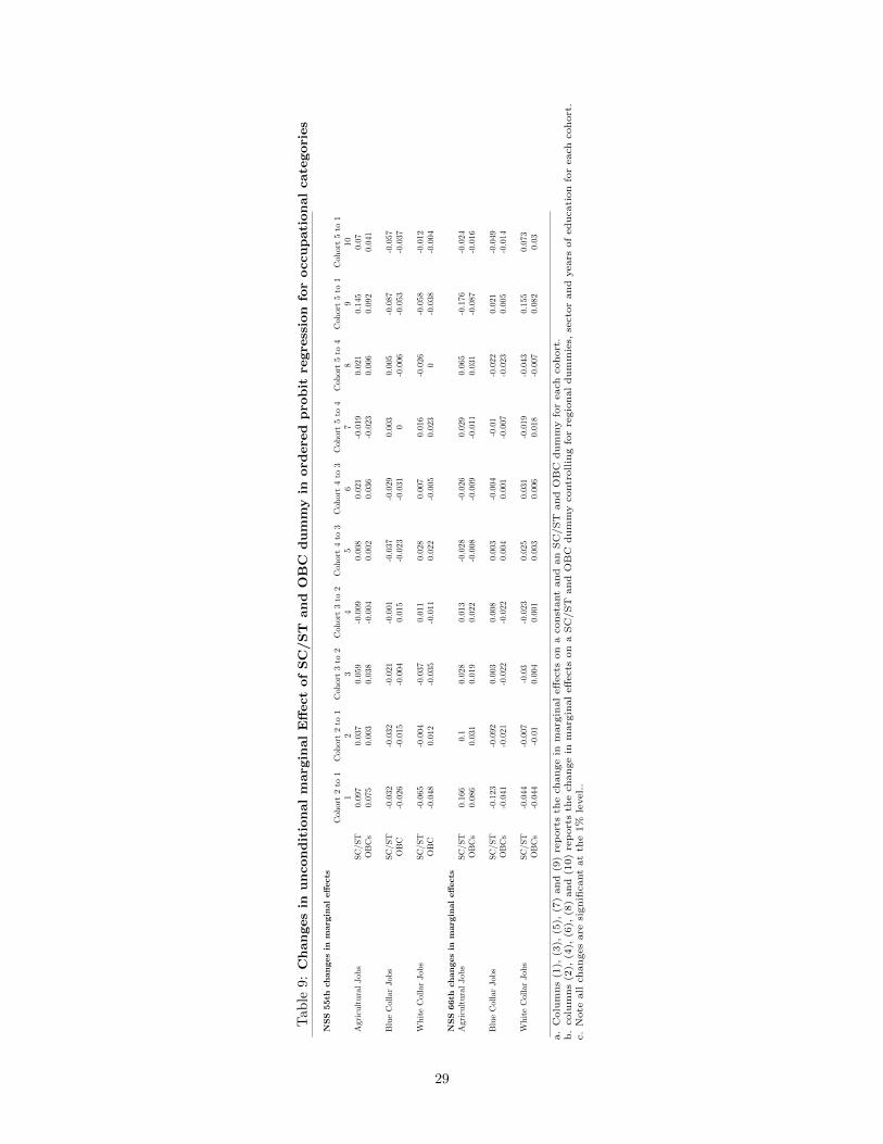
Tab
le9:
Changes
inuncondit
ional
marg
inal
Eff
ect
of
SC
/ST
and
OB
Cdum
my
inord
ere
dpro
bit
regre
ssio
nfo
roccupati
onal
cate
gori
es
NS
S55th
chan
ges
inm
arg
inal
eff
ects
Coh
ort
2to
1C
ohor
t2
to1
Coh
ort
3to
2C
oh
ort
3to
2C
ohort
4to
3C
ohort
4to
3C
ohor
t5
to4
Coh
ort
5to
4C
ohor
t5
to1
Coh
ort
5to
11
23
45
67
89
10A
gric
ult
ura
lJob
sS
C/S
T0.0
97
0.037
0.0
59
-0.0
09
0.0
080.
021
-0.0
190.
021
0.145
0.07
OB
Cs
0.075
0.0
03
0.0
38-0
.004
0.002
0.0
36-0
.023
0.006
0.09
20.
041
Blu
eC
olla
rJob
sS
C/S
T-0
.032
-0.0
32-0
.021
-0.0
01
-0.0
37-0
.029
0.00
30.0
05-0
.087
-0.0
57O
BC
-0.0
26-0
.015
-0.0
04
0.0
15
-0.0
23-0
.031
0-0
.006
-0.0
53
-0.0
37
Wh
ite
Col
lar
Job
sS
C/S
T-0
.065
-0.0
04-0
.037
0.011
0.028
0.0
070.
016
-0.0
26-0
.058
-0.0
12O
BC
-0.0
480.
012
-0.0
35
-0.0
110.
022
-0.0
05
0.023
0-0
.038
-0.0
04
NS
S66th
chan
ges
inm
arg
inal
eff
ects
Agr
icu
ltu
ral
Job
sS
C/S
T0.1
66
0.1
0.028
0.0
13
-0.0
28
-0.0
260.0
29
0.06
5-0
.176
-0.0
24O
BC
s0.
086
0.0
31
0.0
190.
022
-0.0
08
-0.0
09
-0.0
110.
031
-0.0
87-0
.016
Blu
eC
olla
rJob
sS
C/S
T-0
.123
-0.0
920.0
03
0.008
0.0
03-0
.004
-0.0
1-0
.022
0.02
1-0
.049
OB
Cs
-0.0
41-0
.021
-0.0
22
-0.0
22
0.004
0.0
01-0
.007
-0.0
230.
005
-0.0
14
Wh
ite
Col
lar
Job
sS
C/S
T-0
.044
-0.0
07-0
.03
-0.0
23
0.02
50.
031
-0.0
19-0
.043
0.15
50.0
73O
BC
s-0
.044
-0.0
10.
004
0.0
01
0.0
030.
006
0.0
18
-0.0
070.
082
0.03
a.
Colu
mns
(1),
(3),
(5),
(7)
and
(9)
rep
ort
sth
ech
ange
inm
arg
inal
eff
ects
on
aconst
ant
and
an
SC
/ST
and
OB
Cdum
my
for
each
cohort
.b.
colu
mns
(2),
(4),
(6),
(8)
and
(10)
rep
ort
sth
ech
ange
inm
arg
inal
eff
ects
on
aSC
/ST
and
OB
Cdum
my
contr
ollin
gfo
rre
gio
nal
dum
mie
s,se
cto
rand
years
of
educati
on
for
each
cohort
.c.
Note
all
changes
are
signifi
cant
at
the
1%
level..
29
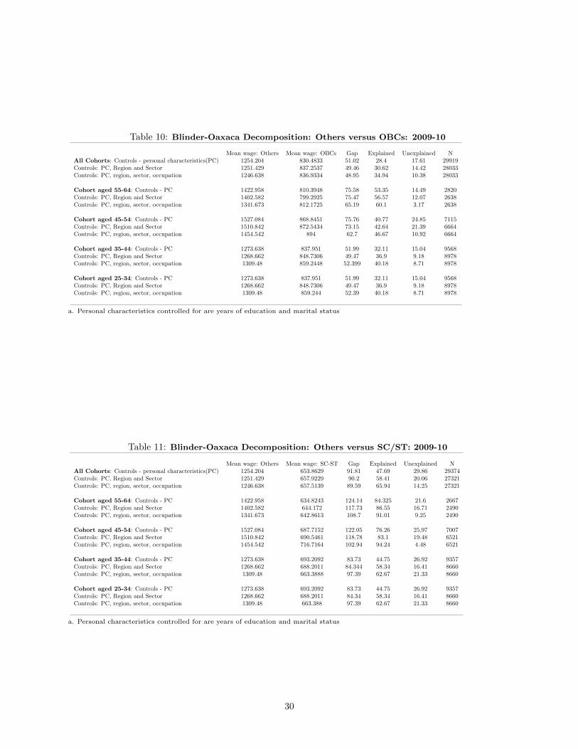
Table 10: Blinder-Oaxaca Decomposition: Others versus OBCs: 2009-10
Mean wage: Others Mean wage: OBCs Gap Explained Unexplained NAll Cohorts: Controls - personal characteristics(PC) 1254.204 830.4833 51.02 28.4 17.61 29919Controls: PC, Region and Sector 1251.429 837.2537 49.46 30.62 14.42 28033Controls: PC, region, sector, occupation 1246.638 836.9334 48.95 34.94 10.38 28033
Cohort aged 55-64: Controls - PC 1422.958 810.3948 75.58 53.35 14.49 2820Controls: PC, Region and Sector 1402.582 799.2925 75.47 56.57 12.07 2638Controls: PC, region, sector, occupation 1341.673 812.1725 65.19 60.1 3.17 2638
Cohort aged 45-54: Controls - PC 1527.084 868.8451 75.76 40.77 24.85 7115Controls: PC, Region and Sector 1510.842 872.5434 73.15 42.64 21.39 6664Controls: PC, region, sector, occupation 1454.542 894 62.7 46.67 10.92 6664
Cohort aged 35-44: Controls - PC 1273.638 837.951 51.99 32.11 15.04 9568Controls: PC, Region and Sector 1268.662 848.7306 49.47 36.9 9.18 8978Controls: PC, region, sector, occupation 1309.48 859.2448 52.399 40.18 8.71 8978
Cohort aged 25-34: Controls - PC 1273.638 837.951 51.99 32.11 15.04 9568Controls: PC, Region and Sector 1268.662 848.7306 49.47 36.9 9.18 8978Controls: PC, region, sector, occupation 1309.48 859.244 52.39 40.18 8.71 8978
a. Personal characteristics controlled for are years of education and marital status
Table 11: Blinder-Oaxaca Decomposition: Others versus SC/ST: 2009-10
Mean wage: Others Mean wage: SC-ST Gap Explained Unexplained NAll Cohorts: Controls - personal characteristics(PC) 1254.204 653.8629 91.81 47.69 29.86 29374Controls: PC, Region and Sector 1251.429 657.9229 90.2 58.41 20.06 27321Controls: PC, region, sector, occupation 1246.638 657.5139 89.59 65.94 14.25 27321
Cohort aged 55-64: Controls - PC 1422.958 634.8243 124.14 84.325 21.6 2667Controls: PC, Region and Sector 1402.582 644.172 117.73 86.55 16.71 2490Controls: PC, region, sector, occupation 1341.673 642.8613 108.7 91.01 9.25 2490
Cohort aged 45-54: Controls - PC 1527.084 687.7152 122.05 76.26 25.97 7007Controls: PC, Region and Sector 1510.842 690.5461 118.78 83.1 19.48 6521Controls: PC, region, sector, occupation 1454.542 716.7164 102.94 94.24 4.48 6521
Cohort aged 35-44: Controls - PC 1273.638 693.2092 83.73 44.75 26.92 9357Controls: PC, Region and Sector 1268.662 688.2011 84.344 58.34 16.41 8660Controls: PC, region, sector, occupation 1309.48 663.3888 97.39 62.67 21.33 8660
Cohort aged 25-34: Controls - PC 1273.638 693.2092 83.73 44.75 26.92 9357Controls: PC, Region and Sector 1268.662 688.2011 84.34 58.34 16.41 8660Controls: PC, region, sector, occupation 1309.48 663.388 97.39 62.67 21.33 8660
a. Personal characteristics controlled for are years of education and marital status
30
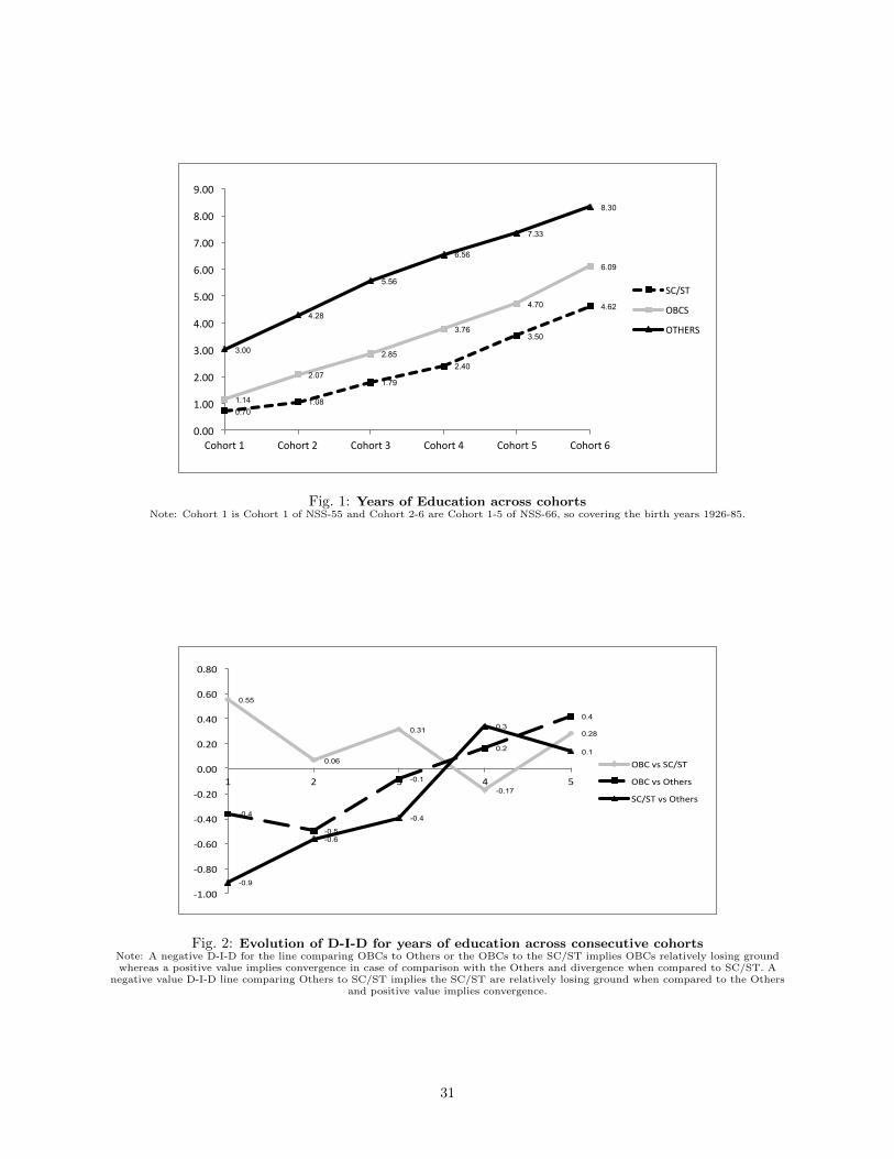
0.70 1.08
1.79
2.40
3.50
4.62
1.14
2.07
2.85
3.76
4.70
6.09
3.00
4.28
5.56
6.56
7.33
8.30
0.00
1.00
2.00
3.00
4.00
5.00
6.00
7.00
8.00
9.00
Cohort 1 Cohort 2 Cohort 3 Cohort 4 Cohort 5 Cohort 6
SC/ST
OBCS
OTHERS
Fig. 1: Years of Education across cohortsNote: Cohort 1 is Cohort 1 of NSS-55 and Cohort 2-6 are Cohort 1-5 of NSS-66, so covering the birth years 1926-85.
0.55
0.06
0.31
-0.17
0.28
-0.4
-0.5
-0.1
0.2
0.4
-0.9
-0.6
-0.4
0.3
0.1
-‐1.00
-‐0.80
-‐0.60
-‐0.40
-‐0.20
0.00
0.20
0.40
0.60
0.80
1 2 3 4 5
OBC vs SC/ST
OBC vs Others
SC/ST vs Others
Fig. 2: Evolution of D-I-D for years of education across consecutive cohortsNote: A negative D-I-D for the line comparing OBCs to Others or the OBCs to the SC/ST implies OBCs relatively losing groundwhereas a positive value implies convergence in case of comparison with the Others and divergence when compared to SC/ST. A
negative value D-I-D line comparing Others to SC/ST implies the SC/ST are relatively losing ground when compared to the Othersand positive value implies convergence.
31
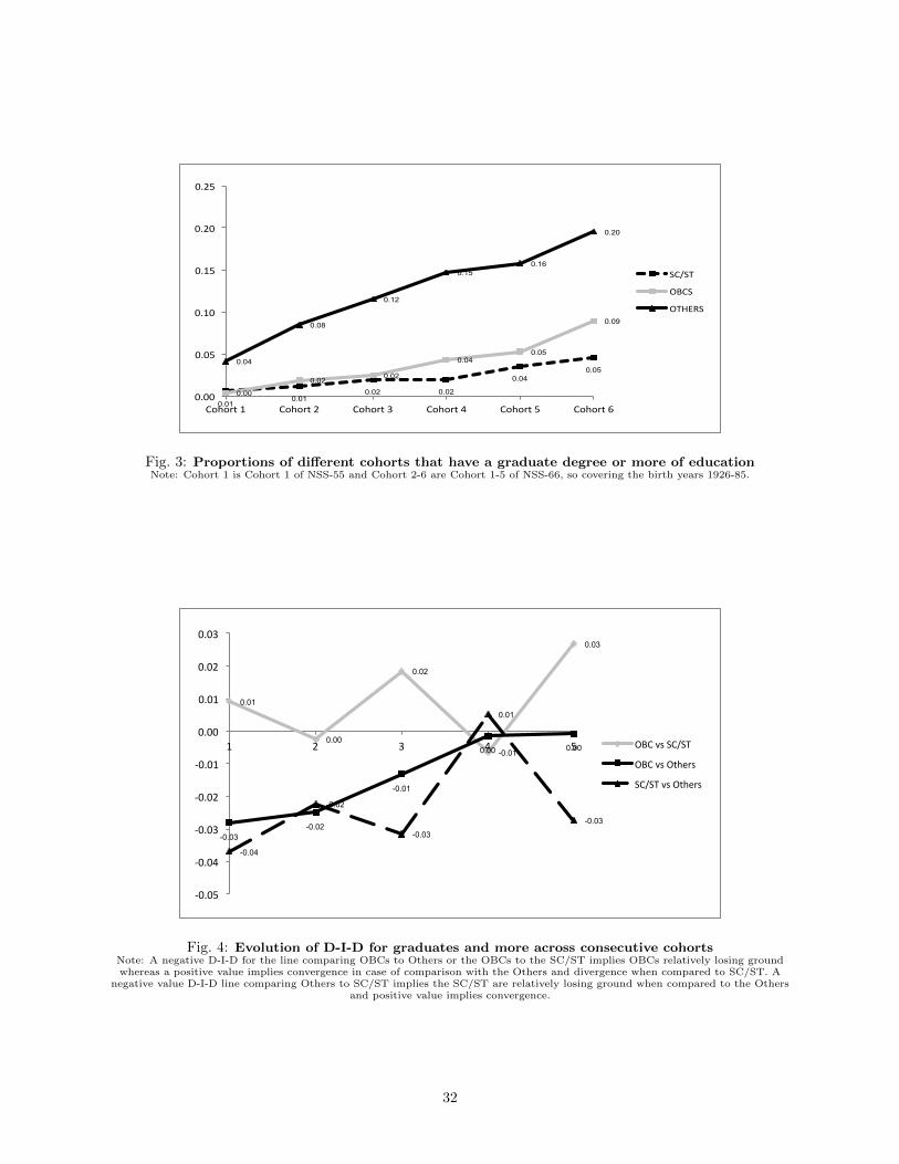
0.01 0.01
0.02 0.02
0.04 0.05
0.00
0.02 0.02
0.04 0.05
0.09
0.04
0.08
0.12
0.15 0.16
0.20
0.00
0.05
0.10
0.15
0.20
0.25
Cohort 1 Cohort 2 Cohort 3 Cohort 4 Cohort 5 Cohort 6
SC/ST
OBCS
OTHERS
Fig. 3: Proportions of different cohorts that have a graduate degree or more of educationNote: Cohort 1 is Cohort 1 of NSS-55 and Cohort 2-6 are Cohort 1-5 of NSS-66, so covering the birth years 1926-85.
0.01
0.00
0.02
-0.01
0.03
-0.03 -0.02
-0.01
0.00 0.00
-0.04
-0.02
-0.03
0.01
-0.03
-‐0.05
-‐0.04
-‐0.03
-‐0.02
-‐0.01
0.00
0.01
0.02
0.03
1 2 3 4 5 OBC vs SC/ST
OBC vs Others
SC/ST vs Others
Fig. 4: Evolution of D-I-D for graduates and more across consecutive cohortsNote: A negative D-I-D for the line comparing OBCs to Others or the OBCs to the SC/ST implies OBCs relatively losing groundwhereas a positive value implies convergence in case of comparison with the Others and divergence when compared to SC/ST. A
negative value D-I-D line comparing Others to SC/ST implies the SC/ST are relatively losing ground when compared to the Othersand positive value implies convergence.
32
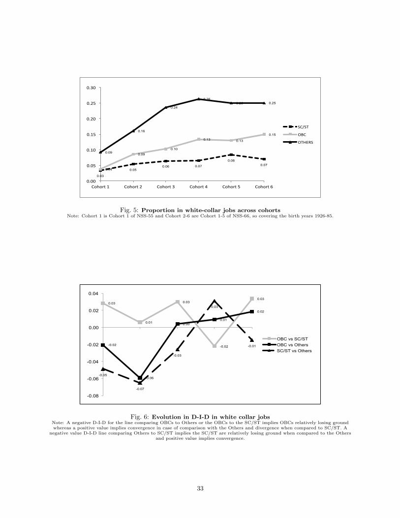
0.03
0.05 0.06 0.07
0.08 0.07
0.04
0.09
0.10
0.13 0.13
0.15
0.09
0.16
0.24
0.26 0.25 0.25
0.00
0.05
0.10
0.15
0.20
0.25
0.30
Cohort 1 Cohort 2 Cohort 3 Cohort 4 Cohort 5 Cohort 6
SC/ST
OBC
OTHERS
Fig. 5: Proportion in white-collar jobs across cohortsNote: Cohort 1 is Cohort 1 of NSS-55 and Cohort 2-6 are Cohort 1-5 of NSS-66, so covering the birth years 1926-85.
0.03
0.01
0.03
-0.02
0.03
-0.02
-0.06
0.00 0.01
0.02
-0.05
-0.07
-0.03
0.03
-0.01
-0.08
-0.06
-0.04
-0.02
0.00
0.02
0.04
OBC vs SC/ST OBC vs Others SC/ST vs Others
Fig. 6: Evolution in D-I-D in white collar jobsNote: A negative D-I-D for the line comparing OBCs to Others or the OBCs to the SC/ST implies OBCs relatively losing groundwhereas a positive value implies convergence in case of comparison with the Others and divergence when compared to SC/ST. A
negative value D-I-D line comparing Others to SC/ST implies the SC/ST are relatively losing ground when compared to the Othersand positive value implies convergence.
33
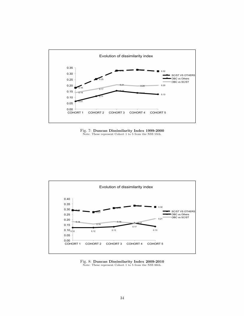
0.18
0.25
0.32 0.33 0.32
0.07
0.11
0.16 0.14
0.13 0.14
0.17
0.21 0.20 0.20
0.00
0.05
0.10
0.15
0.20
0.25
0.30
0.35
COHORT 1 COHORT 2 COHORT 3 COHORT 4 COHORT 5
Evolution of dissimilarity index
SC/ST VS OTHERS OBC vs Others OBC vs SC/ST
Fig. 7: Duncan Dissimilarity Index 1999-2000Note: These represent Cohort 1 to 5 from the NSS 55th.
0.29 0.27
0.31 0.33
0.32
0.12 0.12 0.13
0.17
0.13
0.18 0.16
0.18 0.17
0.21
0.00
0.05
0.10
0.15
0.20
0.25
0.30
0.35
0.40
COHORT 1 COHORT 2 COHORT 3 COHORT 4 COHORT 5
Evolution of dissimilarity index
SC/ST VS OTHERS OBC vs Others OBC vs SC/ST
Fig. 8: Duncan Dissimilarity Index 2009-2010Note: These represent Cohort 1 to 5 from the NSS 66th.
34
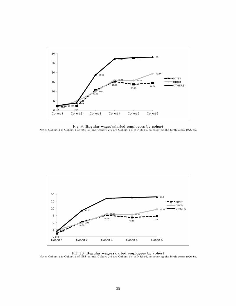
2.1 2.18
10.53
15.18
13.56 14.51
1.66
4.66
9.91
16.04 15.66
19.27
2.33 3.69
18.65
27.02 27.77 28.1
0
5
10
15
20
25
30
Cohort 1 Cohort 2 Cohort 3 Cohort 4 Cohort 5 Cohort 6
SC/ST OBCS OTHERS
Fig. 9: Regular wage/salaried employees by cohortNote: Cohort 1 is Cohort 1 of NSS-55 and Cohort 2-6 are Cohort 1-5 of NSS-66, so covering the birth years 1926-85.
2.18
10.53
15.18 13.56
14.51
4.66
9.91
16.04 15.66
19.27
3.69
18.65
27.02 27.77 28.1
0
5
10
15
20
25
30
Cohort 1 Cohort 2 Cohort 3 Cohort 4 Cohort 5
SC/ST OBCS OTHERS
Fig. 10: Regular wage/salaried employees by cohortNote: Cohort 1 is Cohort 1 of NSS-55 and Cohort 2-6 are Cohort 1-5 of NSS-66, so covering the birth years 1926-85.
35
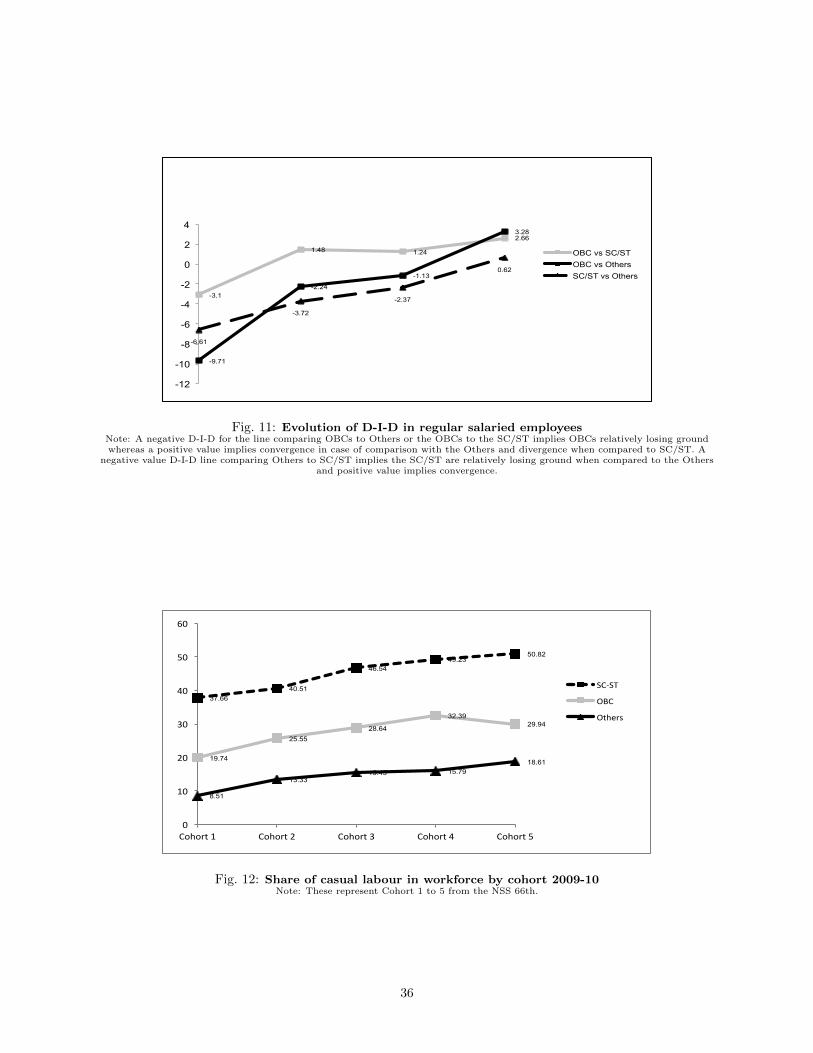
-3.1
1.48 1.24
2.66
-9.71
-2.24
-1.13
3.28
-6.61
-3.72
-2.37
0.62
-12
-10
-8
-6
-4
-2
0
2
4
OBC vs SC/ST OBC vs Others SC/ST vs Others
Fig. 11: Evolution of D-I-D in regular salaried employeesNote: A negative D-I-D for the line comparing OBCs to Others or the OBCs to the SC/ST implies OBCs relatively losing groundwhereas a positive value implies convergence in case of comparison with the Others and divergence when compared to SC/ST. A
negative value D-I-D line comparing Others to SC/ST implies the SC/ST are relatively losing ground when compared to the Othersand positive value implies convergence.
37.66 40.51
46.54 49.23
50.82
19.74
25.55 28.64
32.39 29.94
8.51
13.33 15.45 15.79
18.61
0
10
20
30
40
50
60
Cohort 1 Cohort 2 Cohort 3 Cohort 4 Cohort 5
SC-‐ST
OBC
Others
Fig. 12: Share of casual labour in workforce by cohort 2009-10Note: These represent Cohort 1 to 5 from the NSS 66th.
36
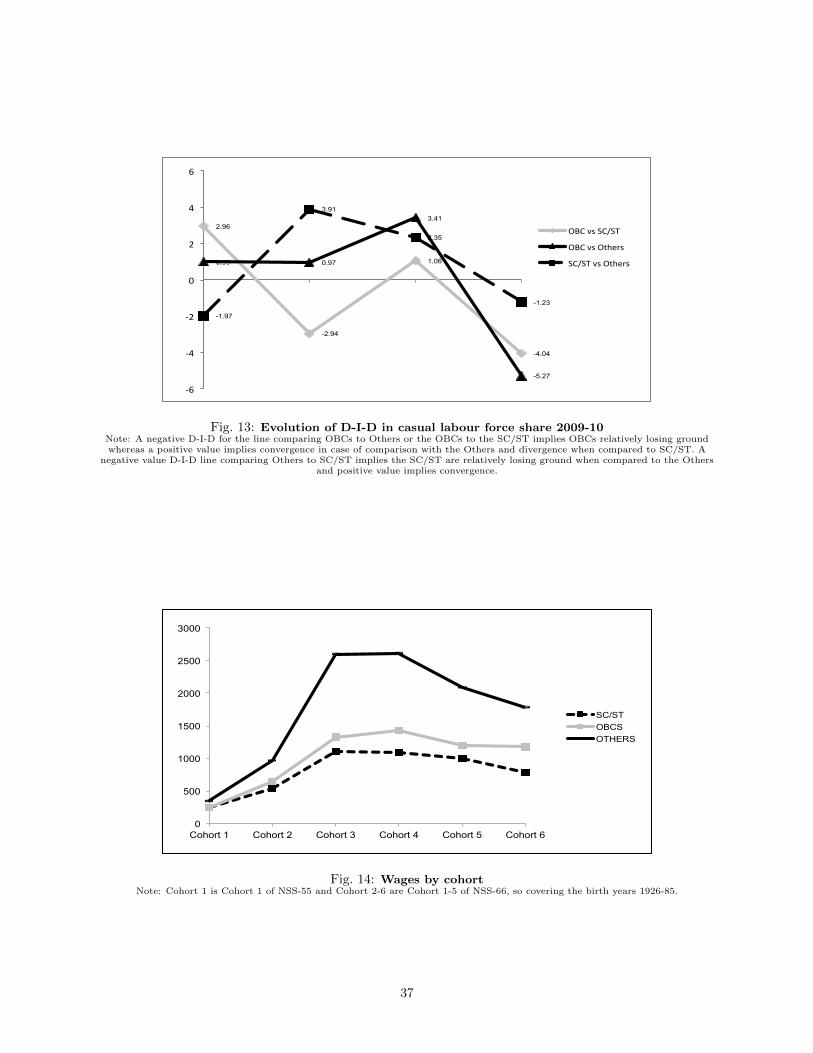
2.96
-2.94
1.06
-4.04
0.99 0.97
3.41
-5.27
-1.97
3.91
2.35
-1.23
-‐6
-‐4
-‐2
0
2
4
6
OBC vs SC/ST
OBC vs Others
SC/ST vs Others
Fig. 13: Evolution of D-I-D in casual labour force share 2009-10Note: A negative D-I-D for the line comparing OBCs to Others or the OBCs to the SC/ST implies OBCs relatively losing groundwhereas a positive value implies convergence in case of comparison with the Others and divergence when compared to SC/ST. A
negative value D-I-D line comparing Others to SC/ST implies the SC/ST are relatively losing ground when compared to the Othersand positive value implies convergence.
0
500
1000
1500
2000
2500
3000
Cohort 1 Cohort 2 Cohort 3 Cohort 4 Cohort 5 Cohort 6
SC/ST OBCS OTHERS
Fig. 14: Wages by cohortNote: Cohort 1 is Cohort 1 of NSS-55 and Cohort 2-6 are Cohort 1-5 of NSS-66, so covering the birth years 1926-85.
37
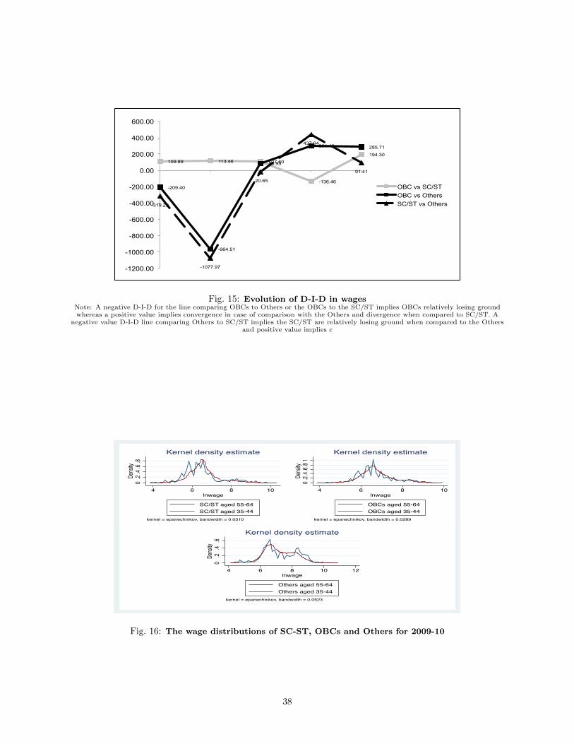
109.89 113.46 107.60
-136.46
194.30
-209.40
-964.51
86.95
301.48 285.71
-319.29
-1077.97
-20.65
437.94
91.41
-1200.00
-1000.00
-800.00
-600.00
-400.00
-200.00
0.00
200.00
400.00
600.00
OBC vs SC/ST OBC vs Others SC/ST vs Others
Fig. 15: Evolution of D-I-D in wagesNote: A negative D-I-D for the line comparing OBCs to Others or the OBCs to the SC/ST implies OBCs relatively losing groundwhereas a positive value implies convergence in case of comparison with the Others and divergence when compared to SC/ST. A
negative value D-I-D line comparing Others to SC/ST implies the SC/ST are relatively losing ground when compared to the Othersand positive value implies c
0.2.
4.6.
8De
nsity
4 6 8 10lnwage
SC/ST aged 55-64SC/ST aged 35-44
kernel = epanechnikov, bandwidth = 0.0310
Kernel density estimate
0.2.4
.6.81
Densi
ty
4 6 8 10lnwage
OBCs aged 55-64OBCs aged 35-44
kernel = epanechnikov, bandwidth = 0.0289
Kernel density estimate
0.2
.4.6
Densi
ty
4 6 8 10 12lnwage
Others aged 55-64Others aged 35-44
kernel = epanechnikov, bandwidth = 0.0523
Kernel density estimate
Fig. 16: The wage distributions of SC-ST, OBCs and Others for 2009-10
38
7 Appendix
7.1 The Blinder-Oaxaca Decomposition Methodology
The detailed methodology can be found in Jann (2008). In this appendix we explain the method intuitively
for those not inclined to go into the technical details. In two independently written pioneering papers,
Blinder (1973) and Oaxaca (1973) outlined the econometric methodology to decompose the average wage
gap between two groups into two components: the explained component, or the part of the wage gap which
can be explained by human capital or endowments (the wage-earning characteristics), and the unexplained
component. The latter is interpreted as a measure of labour market discrimination as it is the part of the wage
gap that remains unaccounted for after all the wage-earning characteristics are accounted for. The basic belief
behind this approach is that wages differ both because of productivity or skill differences between groups
as well as because the market treats the same characteristics differently. What can be observed are only
the actual wage differences; the B-O method artificially separates the endowment/productivity differences
from the treatment or the rate of return effect. The basic Blinder- Oaxaca method suggests substituting
the estimated rates of returns from one group into the estimated wage equation of the other group to
construct counterfactual wage distributions (if there are two groups being compared, as in our paper, there
are two counterfactual wage distributions which get constructed). However, this leads to question of which
counterfactual wage distribution would prevail in the absence of discrimination and one possible alternative
to estimating two separate counterfactuals is to estimate a pooled model over both groups to get the reference
coefficients (which are supposed to represent the non-discriminatory wage structure). We use the pooled
method in the present paper.
7.2 Additional figures and tables
39
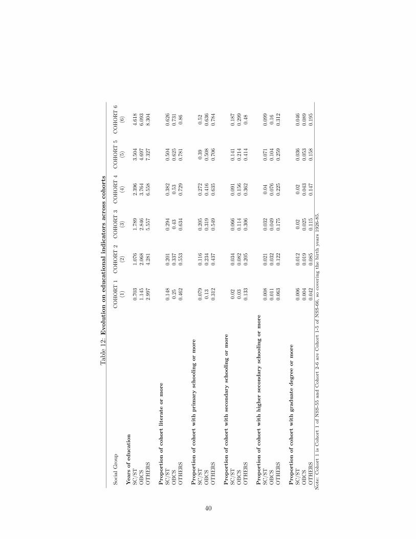
Tab
le12:
Evolu
tion
on
educati
onal
indic
ato
rsacro
sscohort
s
Soci
alG
rou
pC
OH
OR
T1
CO
HO
RT
2C
OH
OR
T3
CO
HO
RT
4C
OH
OR
T5
CO
HO
RT
6(1
)(2
)(3
)(4
)(5
)(6
)Y
ears
of
ed
ucati
on
SC
/ST
0.70
31.0
761.7
892.3
963.
504
4.61
8O
BC
S1.1
452.0
682.
846
3.76
44.
697
6.093
OT
HE
RS
2.997
4.281
5.557
6.55
87.
327
8.30
4
Pro
port
ion
of
coh
ort
lite
rate
or
more
SC
/ST
0.14
80.2
010.2
940.3
820.
504
0.62
6O
BC
S0.
250.
337
0.43
0.5
30.
625
0.731
OT
HE
RS
0.462
0.553
0.634
0.72
90.
781
0.86
Pro
port
ion
of
coh
ort
wit
hp
rim
ary
sch
ooli
ng
or
more
SC
/ST
0.07
90.1
160.2
050.2
720.3
90.
52O
BC
S0.
130.
234
0.31
90.
416
0.50
80.
636
OT
HE
RS
0.312
0.437
0.549
0.63
50.
706
0.78
4
Pro
port
ion
of
coh
ort
wit
hse
con
dary
sch
ooli
ng
or
more
SC
/ST
0.02
0.03
40.
066
0.09
10.
141
0.18
7O
BC
S0.
030.
082
0.11
40.
156
0.21
40.
299
OT
HE
RS
0.133
0.205
0.306
0.36
20.
414
0.48
Pro
port
ion
of
coh
ort
wit
hh
igh
er
secon
dary
sch
ooli
ng
or
more
SC
/ST
0.00
80.0
210.0
320.
040.
071
0.09
9O
BC
S0.0
110.0
320.
049
0.07
60.
104
0.16
OT
HE
RS
0.063
0.122
0.175
0.22
50.
259
0.31
2
Pro
port
ion
of
coh
ort
wit
hgra
du
ate
degre
eor
more
SC
/ST
0.00
60.0
120.
020.
02
0.03
60.
046
OB
CS
0.0
040.0
190.
025
0.04
30.
053
0.089
OT
HE
RS
0.042
0.085
0.115
0.14
70.
158
0.19
5N
ote
:C
ohort
1is
Cohort
1of
NSS-5
5and
Cohort
2-6
are
Cohort
1-5
of
NSS-6
6,
socoveri
ng
the
bir
thyears
1926-8
5.
40
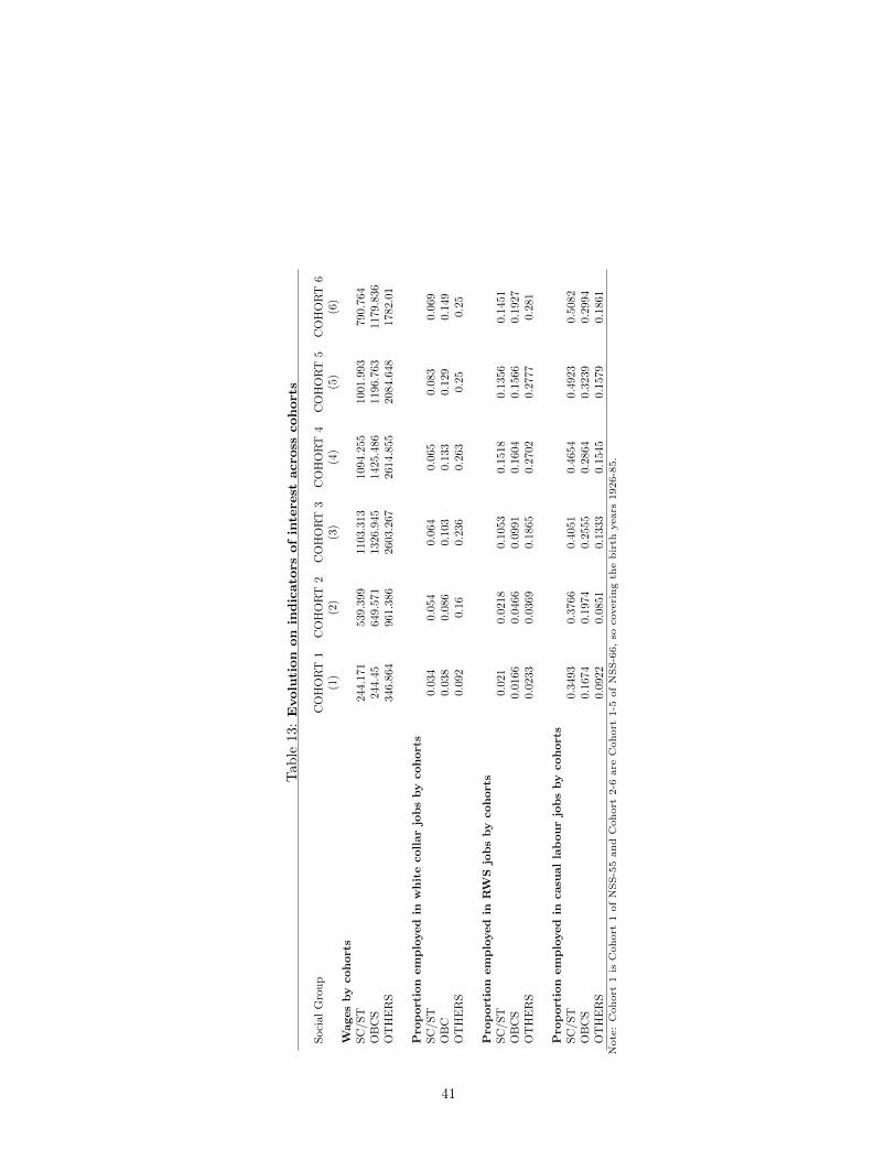
Tab
le13:
Evolu
tion
on
indic
ato
rsof
inte
rest
acro
sscohort
s
Soci
alG
rou
pC
OH
OR
T1
CO
HO
RT
2C
OH
OR
T3
CO
HO
RT
4C
OH
OR
T5
CO
HO
RT
6(1
)(2
)(3
)(4
)(5
)(6
)W
ages
by
coh
ort
sS
C/S
T24
4.1
7153
9.39
911
03.3
1310
94.2
55100
1.99
379
0.76
4O
BC
S24
4.45
649.
571
1326
.945
1425.
486
1196
.763
1179
.836
OT
HE
RS
346.
864
961.
386
260
3.26
726
14.8
55208
4.64
817
82.0
1
Pro
port
ion
em
plo
yed
inw
hit
ecoll
ar
job
sby
coh
ort
sS
C/S
T0.
034
0.05
40.
064
0.06
50.
083
0.0
69O
BC
0.03
80.0
860.
103
0.13
30.
129
0.14
9O
TH
ER
S0.
092
0.1
60.
236
0.26
30.
250.
25
Pro
port
ion
em
plo
yed
inR
WS
job
sby
coh
ort
sS
C/S
T0.
021
0.02
180.1
053
0.1
518
0.1
356
0.14
51
OB
CS
0.01
66
0.046
60.
099
10.
1604
0.15
660.
1927
OT
HE
RS
0.0
233
0.03
69
0.186
50.
270
20.
2777
0.281
Pro
port
ion
em
plo
yed
incasu
al
lab
ou
rjo
bs
by
coh
ort
sS
C/S
T0.
3493
0.37
660.4
051
0.4
654
0.4
923
0.50
82
OB
CS
0.16
74
0.197
40.
255
50.
2864
0.32
390.
2994
OT
HE
RS
0.0
922
0.08
51
0.133
30.
154
50.
1579
0.18
61N
ote
:C
ohort
1is
Cohort
1of
NSS-5
5and
Cohort
2-6
are
Cohort
1-5
of
NSS-6
6,
socoveri
ng
the
bir
thyears
1926-8
5.
41
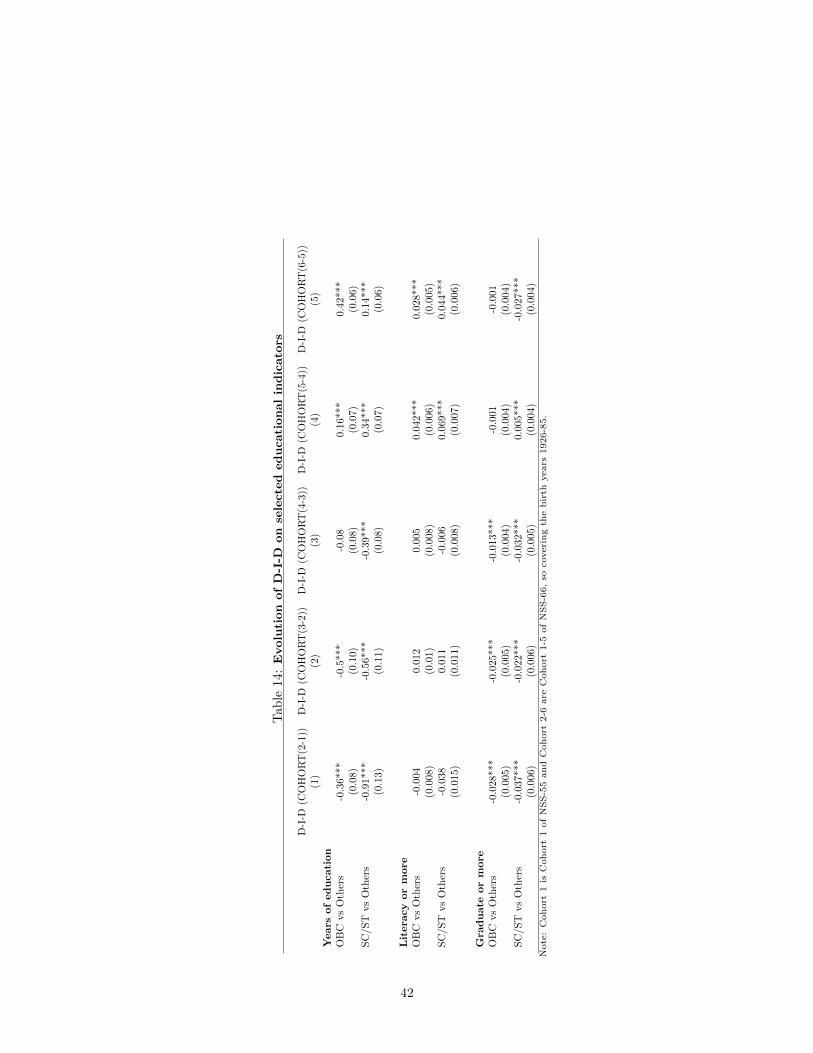
Tab
le14
:E
volu
tion
of
D-I
-Don
sele
cte
deducati
onal
indic
ato
rs
D-I
-D(C
OH
OR
T(2
-1))
D-I
-D(C
OH
OR
T(3
-2))
D-I
-D(C
OH
OR
T(4
-3))
D-I
-D(C
OH
OR
T(5
-4))
D-I
-D(C
OH
OR
T(6
-5))
(1)
(2)
(3)
(4)
(5)
Years
of
ed
ucati
on
OB
Cvs
Oth
ers
-0.3
6***
-0.5
***
-0.0
80.
16*
**0.4
2***
(0.0
8)(0
.10)
(0.0
8)
(0.0
7)
(0.0
6)
SC
/ST
vs
Oth
ers
-0.9
1***
-0.5
6***
-0.3
9***
0.3
4***
0.14
***
(0.1
3)(0
.11)
(0.0
8)
(0.0
7)
(0.0
6)
Lit
era
cy
or
more
OB
Cvs
Oth
ers
-0.0
040.
012
0.0
050.
042**
*0.
028**
*(0
.008
)(0
.01)
(0.0
08)
(0.0
06)
(0.0
05)
SC
/ST
vs
Oth
ers
-0.0
380.
011
-0.0
060.
069**
*0.
044**
*(0
.015
)(0
.011
)(0
.008
)(0
.007
)(0
.006)
Gra
du
ate
or
more
OB
Cvs
Oth
ers
-0.0
28**
*-0
.025*
**-0
.013
***
-0.0
01-0
.001
(0.0
05)
(0.0
05)
(0.0
04)
(0.0
04)
(0.0
04)
SC
/ST
vs
Oth
ers
-0.0
37**
*-0
.022*
**-0
.032
***
0.0
05**
*-0
.027
***
(0.0
06)
(0.0
06)
(0.0
05)
(0.0
04)
(0.0
04)
Note
:C
ohort
1is
Cohort
1of
NSS-5
5and
Cohort
2-6
are
Cohort
1-5
of
NSS-6
6,
socoveri
ng
the
bir
thyears
1926-8
5.
42
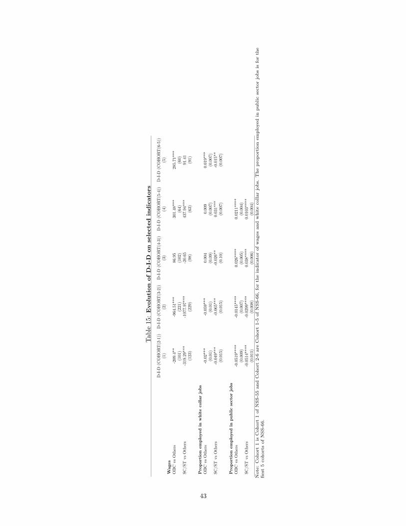
Tab
le15:
Evolu
tion
of
D-I
-Don
sele
cte
din
dic
ato
rs
D-I
-D(C
OH
OR
T(2
-1))
D-I
-D(C
OH
OR
T(3
-2))
D-I
-D(C
OH
OR
T(4
-3))
D-I
-D(C
OH
OR
T(5
-4))
D-I
-D(C
OH
OR
T(6
-5))
(1)
(2)
(3)
(4)
(5)
Wages
OB
Cvs
Oth
ers
-209.
4**
-964
.51*
**86
.95
301.
48***
285.
71*
**(1
01)
(221
)(1
02)
(64)
(60)
SC
/ST
vs
Oth
ers
-319.
29**
*-1
077.
97**
*-2
0.65
437
.94*
**91
.41
(123)
(229
)(9
8)(6
3)(9
1)
Pro
port
ion
em
plo
yed
inw
hit
ecollar
job
sO
BC
vs
Oth
ers
-0.0
2***
-0.0
59***
0.00
40.
009
0.019
***
(0.0
1)(0
.01)
(0.0
9)(0
.007
)(0
.007)
SC
/ST
vs
Oth
ers
-0.0
49*
**-0
.065*
**-0
.026
**0.
031*
**-0
.015
**(0
.015
)(0
.015
)(0
.10)
(0.0
07)
(0.0
07)
Pro
port
ion
em
plo
yed
inp
ub
lic
secto
rjo
bs
OB
Cvs
Oth
ers
-0.0
519**
**-0
.014
5**
**0.
026*
***
0.021
1***
*(0
.009
)(0
.007
)(0
.005
)(0
.004
)SC
/ST
vs
Oth
ers
-0.0
514*
***
-0.0
299*
***
0.03
8***
*0.
0103
****
(0.0
11)
(0.0
08)
(0.0
06)
(0.0
04)
Note
:C
ohort
1is
Cohort
1of
NSS-5
5and
Cohort
2-6
are
Cohort
1-5
of
NSS-6
6,
for
the
indic
ato
rof
wages
and
whit
ecollar
jobs.
The
pro
port
ion
em
plo
yed
inpublic
secto
rjo
bs
isfo
rth
efiest
5cohort
sof
NSS-6
6.
43


![New Page 1 [api.ning.com]api.ning.com/files/w9JIhnUgjg-Lf0kSkTaGPVx7pAjEthi... · Scheduled Castes, Scheduled Tribes, Other Backward Classes (Central List), Persons with Disabilities,](https://static.cupdf.com/doc/110x72/5e41988f49acf2078b11c6ac/new-page-1-apiningcomapiningcomfilesw9jihnugjg-lf0ksktagpvx7pajethi.jpg)