TRANSPORTATION RESEARCH RECORD 1112
Highway Economic Analysis Experiences with the 1985 Highway Capacity Manual
SATISH c. SHARMA, PAWAN J. LINGRAS, AND AL WERNER
Implications of some of the changes suggested in the 1985 Highway Capacity Manual are investigated. The study uses statistics from Alberta Transportation, Edmonton, Canada, as the data base and compares cost-volume curves obtained from the 1965 and the 1985 Highway Capacity Manual. The main conclusion of this investigation is that the application of data and caparity analysis procedures from the 1985 manual produces cost-volume relationships that could conflict with the current practice of designing rural highways when used with the traditional values of other variables, such as vehicle running cost and value of travel time. It Is suggestelf that, In order to reflect the cost of deterioration In service with Increasing traffic volume on two-lane roads, a cost of comfort and convenience should be computed and added to the other components of the user cost. Also examined and discussed is the impact of such new features of the 1985 manual as the driver population factor for multilane roads and the directional spilt of traffic on two-lane roads.
The first edition of the Highway Capacity Manual (HCM) was published by the Bureau of Public Roads (1) in 1950. Despite the fact that the manual was based on a sparse data base and had some well recognized shortcomings, it continued to provide a practical guide to highway capacity analysis until the publication of a second edition in 1965. The 1965 HCM (2), published by the Highway Research Board, reflected vastly improved data bases and procedures, and became widely used throughout the world as the standard for highway capacity and level of service analysis. The latest edition of the manual is a 1985 publication by the Transportation Research Board (3). The procedures for planning, design, and operational analysis included in the 1985 HCM are based on several years of extensive research carried out in the United States and other countries.
Among the new or updated features in the 1985 HCM, whi~h are likely to influence the results of such economic analysis as that carried out in this paper, is information on estimating highway capacity for two-lane and multilane rural highways. Three features of the 1985 manual are considered in this investigation: (a) the driver population factor (f ~ for computing the capacity of freeways and multilane highways; (b) the new speed-volume curves for two-lane roads; and (c) the increase in the ideal capacity of two-lane highways to a maximum of 2,800 passenger cars per hour (pcph), which is a ·-total for both
S. C. Sharma and P. J. Lingras, University of Regina, Regina, Saskatchewan S4S OA2, Canada. A. Werner, Alberta Transportation, 4999 98th Avenue, Edmonton, Alberta T6B 2X3, Canada.
directions-a substantial change from the 1965 HCM's value of 2,000 pcph. It may be noted that the term "driver population" in the 1985 HCM and other recent literature (4) refers to traffic stream characteristics, such as trip purpose and trip length distribution.
The main objective of the analysis presented in this paper is to carry out an economic analysis for investigating the influence of the previously mentioned features of the 1985 HCM. The other objectives of this study are (a) to demonstrate the effect of the driver population or road use type on establishing priorities of highway improvement programming; and (b) to describe a proposed model for the cost of user comfort and convenience, which could be useful in highway economic analysis using the 1985 manual.
HIGHWAY CAPACITY ADJUSTMENT FOR DRIVER POPULATION
The general structure of the capacity analysis procedures for multilane highways in the 1985 HCM remains the same as in the 1965 HCM. A maximum service flow rate can be selected from a table of level of service (LOS) criteria and modifications can be made to reflect any prevailing conditions that are other than ideal. The computation of service flow rate is accomplished by using the following formula:
SFi = MSF; x other factors x Ip (1)
where
SFi = service flow rate under prevailing roadway and traffic conditions;
MSFi = maximum service flow rate for LOS i under ideal conditions;
other factors = factors to adjust for number of lanes, width of lanes, heavy vehicles, and so on; and
Ip = adjustment factor for driver population.
The adjustment factor Ip is used in the 1985 HCM to reflect the influence of driver population on the capacity of freeways and multilane rural highways. It is based on the belief that traffic streams with different characteristics (weekend, recrea-

2
tional, perhaps even midday) use facilities less efficiently than weekday commuter or other regular traffic. An adjustment factor Ip of 1.0 is suggested in the manual for weekdays or commuter type of highway traffic. Au/p range of 0.75- 0.90 is suggested for other types of traffic streams. In a recent article, Sharma et al. (4) elaborate on the factor J;, and recommend a finer and more objective classification of roads according to driver population, which can provide a good basis for making an engineering judgment regarding the selection of a particular J;, value from the range given in the 1985 HCM.
NEW SPEED CURVES AND CAPACITY OF TWO-LANE ROADS
The 1985 HCM's speed-volume curves for two-lane highways are substantially different from those given in the 1965 HCM. A set of the average speed versus volume-to-capacity (V /C) ratio curves obtained from the 1965 and 1985 manuals are shown in Figure I. In the 1985 manual, the speed is much less sensitive to the volume of traffic, compared to the 1965 manual.
110
100
90
80
::c 70
' :E 60 ~
0 50 w w 40 0.. (/)
30
20
10
THE NEW HCM, 20% NO PASSING ZONE, DIRECTIONAL DISTRIBUTION 50/50
........... I ' ' ........... ........
........ ........
j'' ...... 1965 HCM, 80% PASSING ......_'
SIGHT DISTANCE ......_
0.1 0.2 03 04 D~ 06 Q7 08 09 I~
V/C RATIO
FIGURE 1 Relatlonshlp between average speed and V/C ratio on two-lane highways.
According to the 1985 HCM, under ideal conditions, the capacity of Lwo-lan~ roads is a total of 2,800 pcph in both directions, which is a substantial mcrease trom tne i 9ti5 HCM's 2,000 value. The ideal conditions in the 1985 manual include a 50/50 directional distribution of traffic. As given in Table l, the capacity of two-lane rural highways varies with directional distribution, and reduces as the split moves away from 50/50 to a minimum value of 2,000 pcph when the split is 100/0.
TRANSPORTATION RESEARCH RECORD 1112
TABLE 1 CAPACITY OF TWO-LANE ROADS AS A FUNCTION OF DIRECTIONAL SPLIT
Total Directional Capacity Ratio of Capacity Split (pcph) to Ideal Capacity
50/50 2,800 1.00 60/40 2,650 0.94 70(30 2,500 0.89 80/20 2,300 0.83 90/10 2,100 0.75
100/0 2,000 0.71
STUDY DATA AND METHOD OF ANALYSIS
Some of the major critical elements that need to be considered in the road sizing and improvement programming (the subject area of the present analysis) are (a) traffic variables, such as traffic stream characteristics, volume of traffic, vehicle classification, and average travel speed; (b) geometric design variables, such as road standard type, design speed, percentage of no-passing zones, and capacity; (c) economic variables, such as cost of highway construction, maintenance, travel time, accidents, and vehicle running costs; and (d) sociopolitical variables, such as community goals and objectives, and user preferences. All of these factors are considered in this analysis using Alberta Transportation (the highway agency for the Province of Alberta, Canada) statistics as the data base. For the purpose of a comparative cost analysis, the speed-volume curves and capacity calculations, which are prerequisites to the determination of the road user costs, are based on both the 1985 and the 1965 HCMs .
Highway Traffic Data
The road user's perspective or road use variable-the terms "road use" and "driver population" are used interchangeably to reflect the traffic stream characteristics-was included in the present analysis by grouping the roads using a previously developed method (4), which is based on temporal volume variations and the traffic stream characteristics of trip purpose and trip length distribution. The road system under investigation was classified into six main types; however, for the sake of simplicity, the analyses for (a) regional commuter, (b) rural Jong distance, and (c) long distance/recreational types ofroutes are included in this paper. The typical sites representing these three road classes in Alberta are as follows:
regional commuter segment of Highway 3 east of Lethbridge; 2. The PTC site C243 located on a rural long distance
portion of the Trans-Canada Highway west of Brooks; and 3. The PTC site C249 located on a rural long distance/
recreational portion of the Trans-Canada Highway in the Banff National Park.
Sharma et al. 3
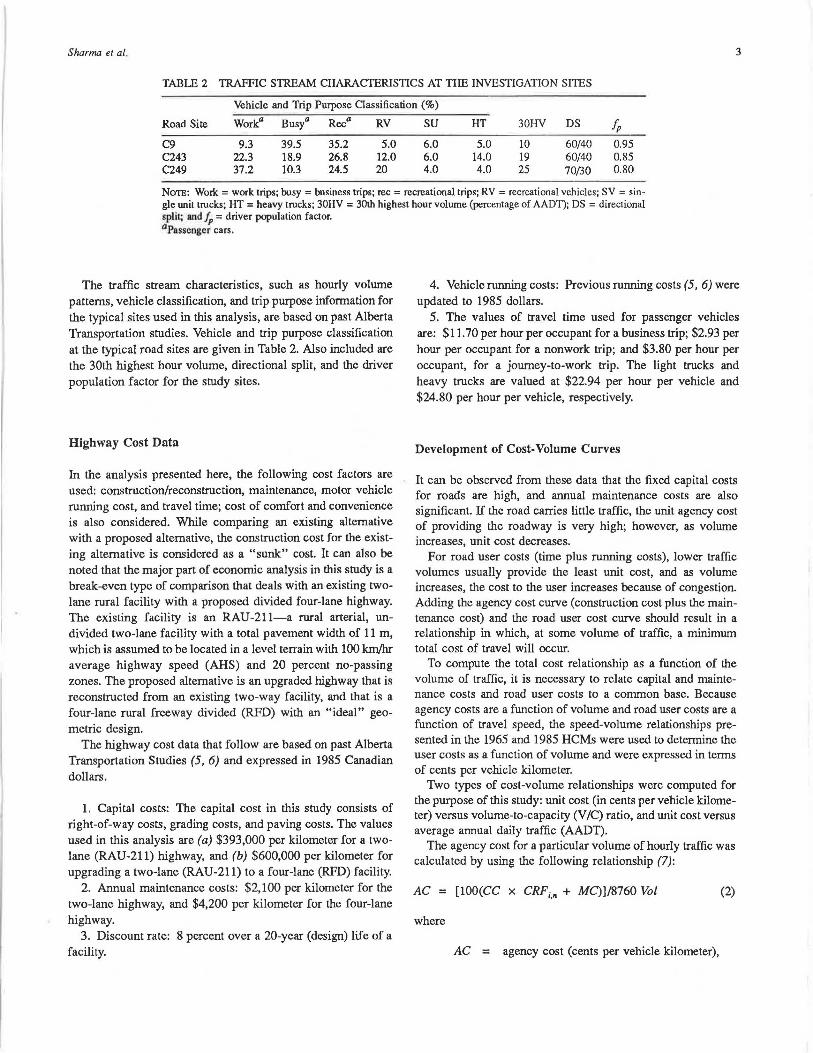
TABLE 2 TRAFFIC STREAM CHARACTERISTICS AT THE INVESTIGATION SITES
Vehicle and Trip Purpose Classification(%)
Road Site Work" Busy a Rec a RV SU HT 30IN DS Ip C9 9.3 39.5 35.2 5.0 6.0 5.0 10 60/40 0.95 C243 22.3 18.9 26.8 12.0 6.0 14.0 19 60/40 0.85 C249 37.2 10.3 24.5 20 4.0 4.0 25 10(30 0.80
Norn: Work = work trips; busy = business trips; rec = recreational trips; RV = recreational vehicles; SV = single unit trucks; HT = heavy trucks; 30HV = 30th highest hour volume (percentage of AADT); DS = directional split; and fp = driver population factor. aPassengcr cars.
The traffic stream characteristics, such as hourly volume patterns, vehicle classification, and trip purpose information for the typical sites used in this analysis, are based on past Alberta Transportation studies. Vehicle and trip purpose classification at the typical road sites are given in Table 2. Also included are the 30th highest hour volume, directional split, and the driver population factor for the study sites.
Highway Cost Data
In the analysis presented here, the following cost factors are used: construction/reconstruction, maintenance, motor vehicle running cost, and travel time; cost of comfort and convenience is also considered. While comparing an existing alternative with a proposed alternative, the construction cost for the existing alternative is considered as a "sunk" cost. It can also be noted that the major part of economic analysis in this study is a break-even type of comparison that deals with an existing twolane rural facility with a proposed divided four-lane highway. The existing facility is an RAU-211-a rural arterial, undivided two-lane facility with a total pavement width of 11 m, which is assumed to be located in a level terrain with 100 km/hr average highway speed (AHS) and 20 percent no-passing zones. The proposed alternative is an upgraded highway that is reconstructed from an existing two-way facility, and that is a four-lane rural freeway divided (RFD) with an "ideal" geometric design.
The highway cost data that follow are based on past Alberta Transportation Studies (5, 6) and expressed in 1985 Canadian dollars.
1. Capital costs: The capital cost in this study consists of right-of-way costs, grading costs, and paving costs. The values used in this analysis are (a) $393,000 per kilometer for a twolane (RAU-211) highway, and (b) $600,000 per kilometer for upgrading a two-lane (RAU-211) to a four-lane (RFD) facility.
2. Annual maintenance costs: $2,100 per kilometer for the two-lane highway, and $4,200 per kilometer for the four-lane highway.
3. Discount rate: 8 percent over a 20-year (design) life of a facility.
4. Vehicle running costs: Previous running costs (5, 6) were updated to 1985 dollars.
5. The values of travel time used for passenger vehicles are: $11. 70 per hour per occupant for a business trip; $2.93 per hour per occupant for a nonwork trip; and $3.80 per hour per occupant, for a journey-to-work trip. The light trucks and heavy trucks are valued at $22.94 per hour per vehicle and $24.80 per hour per vehicle, respectively.
Development of Cost-Volume Curves
It can be observed from these data that the fixed capital costs for roads are high, and annual maintenance costs are also significant. If the road carries little traffic, the unit agency cost of providing the roadway is very high; however, as volume increases, unit cost decreases.
For road user costs (time plus running costs), lower traffic volumes usually provide the least unit cost, and as volume increases, the cost to the user increases because of congestion. Adding the agency cost curve (construction cost plus the maintenance cost) and the road user cost curve should result in a relationship in which, at some volume of traffic, a minimum total cost of travel will occur.
To compute the total cost relationship as a function of the volume of traffic, it is necessary to relate capital and maintenance costs and road user costs to a common base. Because agency costs are a function of volume and road user costs are a function of travel speed, the speed-volume relationships presented in the 1965 and 1985 HCMs were used to determine the user costs as a function of volume and were expressed in terms of cents per vehicle kilometer.
Two types of cost-volume relationships were computed for the purpose of this study: unit cost (in cents per vehicle kilometer) versus volume-to-capacity (V/C) ratio, and unit cost versus average annual daily traffic (AADT).
The agency cost for a particular volume of hourly traffic was calculated by using the following relationship (7):
AC = [lOO(CC x CRF;,,. + MC)]/8760 Vol (2)
where
AC = agency cost (cents per vehicle kilometer),
4
cc = capital cost (dollars per kilometer), CRF;,,. = capital recovery factor for interest rate i
and useful facility life of n years, MC = annual maintenance cost (dollars per
kilometer), and Vol = volume of traffic (vehicles per hour).
The first step in determining the vehicle running cost was to calculate the V /C ratio for a particular hourly volume of travel and the existing road traffic and design conditions. The speed of travel was then estimated from the speed-volume curves presented in the 1965 and 1985 HCMs (2, 3). Finally, the vehicle running costs were obtained from the empirically derived tables of running costs at various speeds (5, 6).
The denominator of the V/C ratio [e.g., the capacity (C) of a road facility] was calculated by using the methods given in the 1965 and 1985 HCMs.
The travel time cost for a given traffic strca...9Il was calculated by using the following relationship (7):
TC = 100 1W[(l/S) - (l/AHS)] (3)
where
TC = travel time cost (cents per vehicle kilometer), 1W = weighted mean travel time cost for the
various types of vehicles in the traffic stream (dollars per hour),
AHS = the average highway speed or the desired speed of travel (kilometers per hour), and
S = space mean speed of travel possible at a given volume of travel (kilometers per hour).
27
26
~ ~
I J: ..... > 25 .......
.......
I-(/)
0 u
24
1,~,~-OS= 50 ,50
23 0.0 0.2 0.4 0.6 0 .8
V/C RATIO
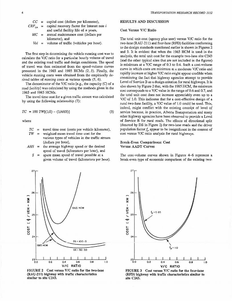
FIGURE 2 Cost versus V/C ratio for the two-lane (RAU-211) highway with traffic characteristics similar to site C243.
1.0
TRANSPORTATION RESEARCH RECORD 1112
RESULTS AND DISCUSSION
Cost Versus V /C Ratio
The total unit cost (agency plus user) versus V/C ratio for the two-lane (RAU-211) and four-lane (RFD) facilities conforming to the design standards mentioned earlier is shown in Figures 2 and 3. It is evident that when the 1965 HCM is used in the analysis, the total unit cost for the example two-lane site C243 (and the other typical sites that are not included in the figures) is minimum at a V/C range of 0.3 to 0.4. Such a cost-volume curve in which costs are minimum at a moderate V/C ratio and rapidly increase at higher V/C ratio might appear credible when considering the fact that highway agencies attempt to provide Level of Service B as a design criterion for rural highways. It is also shown by Figure 2 that, with the 1985 HCM, the minimum cost corresponds to a V /C value in the range of 0.6 and 0. 7, and the total unit cost does not increase appreciably even up to a V/C of 1.0. This indicates that for a cost-effective design of a rural two-lane facility, a V /C value of 1.0 could be used. This, indeed, might conflict with the existing concept of level of service because, in practice, Alberta Transportation and many other highway agencies have been observed to provide a Level of Service B for rural roads. The effects of directional split (denoted by DS in Figure 2) for two-lane roads and the driver population factor Ip appear to be insignificant in the context of cost versus V/C ratio analysis for rural highways.
Break-Even Comparisons: Cost Versus AADT Curves
The cost-volume curves shown in Figures 4-6 represent a break-even type of economic comparison of the existing two-
27
26
~ ~
I J: ..... > 25 .......
.......
I-(/)
0 u
24
,,[ \ fp = I 0
0.0 0.2 0.4 0.6 0.8 1.0
V/C RATIO FIGURE 3 Cost versus V/C ratio for the four-lane (RFD)" highway with traffic characteristics similar to site C243.

Sharma et al.
24
23
:IE 22 ~
I ::c LL.I > 21 ..... .....
t; 20 0 <...>
19
I I I I I I I I
LEGEND ---- 1965 HCM
---- 1985 HCM
EXISTING TWO- LANE HIGHWAY
/ /
/
I I
I /
1s ~~~~~~~~~-'-~~~~-L-~~~~-'-~~~
0 10,000 20,000 30,000 40,000
VOLUME ( AADT)
FIGURE 4 Cost versus AADT curves for the regional commuter site C9.
5
lane facility and the proposed four-lane alternative. In all these figures, the x-axis is the volume of traffic (AADT) in vehicles per day, and the y-axis is the unit cost (cents per vehicle kilometer) corresponding to the 30th highest hour volume for an AADT volume shown on the x-axis. Usually, in the case of break-even comparisons, the x-axis represents the level of
output for the alternatives to be compared. The AADT is used in the present context because it is the most commonly used and easily understood measure of traffic volume. As mentioned earlier, the capital cost for the existing two-lane alternative is considered as a "sunk" cost; the only agency cost in this case is the maintenance cost.
21 0L._~~-5-0~0-0~~~,o-,0Lo_o~~-,-5~,0~0~0~~2=0~.=00=0~~~2~s~.o~o~o:--
VOLUME ( AAOT )
FIGURE 5 Cost versus AADT curves for the long-distance site C243.

6 TRANSPORTATION RESEARCH RECORD 1112
24
I LEGEND
I ---- 1965 HCM 23
:E :lll::
22 J: w > ...... ~
21
..... (/)
0 0
20
19
I I I
I I
I
EXISTING TWO-LANE HIGHWAY
1985 HCM
/ /
/ --
5000 10,000 15,000
VOLUME ( AADT )
FIGURE 6 Cost versus AADT curves for the long-distance/ recreational site C249.
It is apparent that the break-even points derived from the application of the 1985 manual occur at a much higher value of AADT as compared to the 1965 manual. For example, in the case of the regional commuter site C9, a break-even in the costs for the two study alternatives results in an AADT value of 18,500 vehicles per day using the 1985 manual as compared to an AADT value of 7,000 for the 1965 manual. The generally insensitive nature of the new speed curves (3), with respect to the volume of traffic, and a substantial increase in the "ideal" capacity for two-lane roads in the 1985 manual are mainly responsible for such a wide difference in the break-even points.
Another observation that can be made from Figures 4-6 is the effect of road type on cost-volwne curves and the resulting break-even points. Because of their differences in the 30th highest hourly volwne (expressed in percent of AADT), the study sites C9, C243, and C249 exhibit different rates of cost increase beyond the AADT range where the total cost minimization occurs.
The study results pertaining to the value of AADT yielding a break-even situation between the two alternatives were tested
by comparing them with the actual practice of upgrading twolane roads in Alberta. It may be noted that upgrading of twolane roads to three- or four-lane facilities has not been definitive under Alberta Transportation policy to date. In the past, facilities have been reconstructed on the basis of need, as dictated by traffic demand and safety. In one report (8), Alberta Transportation indicated that "expansion to four-lanes will not be undertaken until volumes reach the 6,000 lo 8,000 AADT range." However, since the time of that report, the province has received a large number of user complaints about the poor level of service provided by some of the two-lane roads carrying volumes in the AADT ranges of 2,000 to 4,000 vehicles per day. In many such cases, requests were made to upgrade these roads to the four-lane standard.
Table 3 includes AADT estimates for upgrading two-Jane roads and compares the actual practice by Alberta Transportation and the break-even analysis results from Figures 4-6. The theoretical results correctly indicate the difference in the needs for upgrading the various types of roads at different AADT levels. It is interesting to note that the actual practice followed
TABLE 3 AADT ESTIMATES FOR UPGRADING TWO-LANE ROADS: ALBERTA PRACTICE VERSUS THEORETICAL RESULTS
Actual Alberta Theoretical Results
Road Type Practice 1965 HCM 1985 HCM
Regional commuter 9,000-10,000 7,000 18,500 Rural long distance 4,000-5,000 5,500 13,000 Long distance/recreational 3,000-4,000 3,250 9,000

Sharma et al.
by Alberta Transportation is much closer to the results obtained for the 1965 manual as compared to the results for the 1985 manual. The data given in Table 3 imply that, with a cost model such as that used in this study, a project justifiable from the point of view of the 1965 manual can be found unacceptable using the 1985 manual. In fact, it can be said that the breakeven points or AADT values derived from the use of 1985 HCM are too high, and, as such, the analysis cannot be used as an appropriate model for highway improvement programming.
Cost of Comfort and Convenience
The apparent underestimation of the road user costs for twolane roads, and the overestimation of break-even points associated with the 1985 HCM can be easily understood by considering the use of "percent time delay" in this manual as the primary measure of service quality for two-lane highways-the other two being average travel speed and capacity utilization. The computations of economic costs shown in Figure 2 and Figures 4 through 6 take into account only speed of travel and capacity utilization (or V/C ratio) in the manner used before the publication of the 1985 HCM. The "percent time delay" aspect of the level-of-service analysis is not considered in the economic cost calculations. It is because of this exclusion of "percent time delay" consideration from the economic calculations and the new speed-volume relationship that the costvolume curves obtained from the 1985 HCM are insensitive to traffic volume and do not seem to properly reflect the deterioration in level of service with increases in traffic volume or V /C ratio.
The measure of "percent time delay" is difficult to obtain directly in the field. However, as indicated in the 1985 manual, for field studies, it can be represented in percentage of vehicles traveling at headways of less than 5 sec. The 1985 HCM points out that as volume approaches capacity on two-lane roads, passing demand greatly exceeds passing capacity, which results in a buildup of platoons, and motorists are delayed almost 100 percent of the time. Although the speeds may be relatively high and near capacity, driver frustrations and strain could be intolerable if the platoons routinely existed for long periods of time.
It appears from the preceding discussion that, in order to achieve cost-volume curves that are capable of appropriately reflecting the cost of user congestion, the computations of user costs employing the 1985 HCM should also involve some consideration of motorists' hardship associated with platooning and passing maneuvers on two-lane rural roads. The "percent time delay" parameter in the 1985 manual is intended to be used for level of service analysis, but other factors such as cost of comfort and convenience may be used as a practical measure in highway economic analysis.
A review of the existing state of opinion (3, 7, 9, JO) indicates that any generalized model, in order to provide a measure of comfort and convenience, should cover such factors as (a) the relative importance of driving comfort as perceived by road users, (b) the unsatisfied demand (overtaking demand minus actual overtaking) curves (JO), (c) "percent time delay" curves (3), (d) type of road use (7), (e) V/C ratio (9), (f) desired highway speed, and (g) vehicle classification. Based on these factors, several generalized mathematical models were investi-
7
gated. The following model seems to encompass satisfactorily the foregoing considerations ( 11 ):
CCC = A(V/C)8 (4)
where CCC is the cost of comfort and convenience, and A and B are the model parameters. A detailed description of the model parameters and their calibration is given elsewhere (11 ).
For a brief interpretation of this model and its parameters, the right-hand side of the equation can be split into two parts: the expression (V /C)8
, termed a discomfort and inconvenience index (Dm, and parameter A.
The Dil can be taken to be a relative measure of discomfort and inconvenience as perceived by an average user, and is expressed on a scale of 0.0-1.0, 0.0 being the minimum and 1.0 being the maximum discomfort and inconvenience. Shown in Figure 7 is a plot of the Dil versus V/C curves for different values of B greater than 0.0. The DII curves indicate that (a) the discomfort and inconvenience as perceived by an average user will increase with increasing traffic volume (V/C ratio) and reach a maximum value when V/C equals 1.0, that is, at capacity; (b) except for the value of V/C equal to 1.0, the Dil
0
x UJ 0 z UJ 0 z UJ
z UJ > z 0 0 z
0 z ct .,_ a: 0 LI-~ 0 0 (/)
0
1,0
0. 9
08
0 .7
0 ,6
05
0 .4
0.3
0.2
0 1
0 . 1 0 .2 0 . 3 0.4 0.5 0 6 0 .7 08 0 ,9 I 0
V/C RATIO
FIGURE 7 Effect of parameter Bon discomfort and inconvenience Index.
value for a particular value of V/C increases as the value of B decreases; and (c) the DII value remains the same at 1.0 for V/C equal to 1.0 for all values of B.
Road users making work trips of short distances are usually presumed to have a higher degree of acceptance of congestion, and, therefore, lower expectations of comfort and convenience. On the other hand, users making long-distance trips presumably accept congestion to a lesser degree, and, therefore, expect higher degrees of comfort and convenience. On the basis of

8 TRANSPORTATION RESEARCH RECORD 1112
28
27
~ 26 ::ii::
::c LL.I > 25 ......
PROPOSEO FOUR - LANE ~ HIGHWAY
I- \ Cf) 24 0 (.)
23 FXISTING TWO- LANE
HIGHWAY
VOLUME ( AADT)
FIGURE 8 Cost versus AADT curves for C243 using the 1985 HCM and the cost of comfort and convenience model.
such observations, B can be interpreted as the user's expectancy of the perceived comfort and convenience attached to a highway facility and expected driving conditions; the lower the value of B the higher the expected conditions.
The parameter A may be considered as the maximum perceived monetary value attached to the maximum discomfort and inconvenience (in cents per vehicle kilometer) that occurs at a V/C ratio equal to 1.0, which is the cost that a user is willing to bear in order to achieve the level of comfort and convenience from traveling at a desired speed. Depending on local conditions, such as socioeconomic characteristics, attitudes, perception of preferences, and expectations of the community of users or drivers using the transportation facility, the magnitude of A can be estimated by subjectively assigning a weight to the attribute of comfort and convenience. For example, based on a previous household survey (12) the value of A was made equal to 50 percent of out-of-pocket (or fuel plus oil) cost in the case of the present investigation.
It can be noted that the CCC model (Equation 4) is developed with the intention of using it for two-lane rural highways; the cost value given by this model is assumed mainly to be a measure of the discomfort and inconvenience caused by the phenomena of platooning and overtaking. For this reason, the CCC model is applied only to the existing two-lane alternative and not Lo the four-lane alternative.
While keeping the value of parameter A constam (ac a 50 percent level of the out-of-pocket cost), the effect of parameter B is shown in Figure 8, which is drawn for the study site C243 using the 1985 HCM data. The value of B equal to 2.0 seems to yield the break-even results that conform to the actual practice of upgrading two-lane roads in Alberta, that is, a break-even AADT range of 4,000 to 5,000 in the case of long-distance sites (Table 3). A similar calibration for the other study sites resulted in (a) B equal to 2.5 for the regional corr1n1uter site C9, a...11d (b) B equal to 1.5 for the long-distance/recreational site C249.
The cost versus V /C curves for the different road sites obtained by the 1985 HCM, and the proposed cost of comfort and convenience model are shown in Figure 9. It is evident from this that the inclusion of the cost of comfort and convenience in the analysis gives the desired results that seem to conform to the practice of providing Level of Service B (or C) in designing rural highways. As shown by Figure 9, the high-
27
26
25
::i ::ii::
I 24
::c LL.I > 23 ......
-t:f-
I-Cf)
0 (.)
21
~:[ C9
0 .0 0.2 0.4 0 .6 0 .8
V/C RATIO FIGURE 9 Cost versus V/C ratio for the two-Jane roads using the 1985 HCM !l.nd the cost of comfort and convenience model.
1.0

Sharma et al.
way cost starts increasing rapidly beyond a V /C range of 0.4 to 0.6.
Effect of the Driver Population Factor
The only difference between the cost-volume curves for fourlane highways using the 1985 and the 1965 manuals is that the 1985 manual talces into account the traffic stream characteristics by applying the factor fe in capacity calculation. It can be seen from Figures 4-6 that, ror four-lane highways, the population factor fp causes an upward shift in the cost-volume curve at a high volume of traffic. But this does not seem to significantly affect the results of brealc-even analysis carried out here for upgrading of two-lane roads to four-lane standards. However, this factor is likely to influence the results of other types of transportation analyses involving capacity and level of service for multilane highways.
Effect of the Directional Distribution
The 1985 HCM takes into account the effect of directional distribution of traffic on the highway capacity analysis for twolane roads. The analysis carried out for this paper indicated that a significant difference in the location of the break-even point would result if the two extreme values of the split (100/0 and 50/50) were compared. However, the study results also showed that a modest variation (such as a± 10 percent change) in the directional split would not have a significant impact on highway economic analysis.
CONCLUSIONS
The main conclusions of this study are as follows:
1. The economic analysis of this study shows that the application of the 1985 HCM data and capacity analysis procedure for two-lane roads would require the use of some additional quantifiable variable reflecting the cost of deterioration in service with increasing traffic volume. It is suggested in this paper that a cost of comfort and convenience should be computed and added to the other components of the user cost.
2. The driver population factor fp causes an upward shift in the cost-volume curves, and hence it is likely to influence the results of some transportation analyses involving economic comparisons for multilane highways.
3. The directional split of traffic is an important consideration in the highway capacity analysis for two-lane roads. However, the results of this study indicate that the variations in the range of± 10 percent in directional split would not significantly affect economic analysis.
9
4. Road use type is a significant factor that must be considered for highway improvement programming from both the cost-effectiveness and users' perspectives.
5. The break-even comparison curves developed in this study and the actual practice followed by Alberta Transportation indicate that the AADT can be used as a good criterion for cost-effective and user-oriented upgrading of two-lane roads.
ACKNOWLEDGMENTS
The authors are grateful to Alberta Transportation for providing the necessary data. The observations and views presented in this are strictly the authors' own. The upgrading criteria presented are not formal Alberta Transportation policies. The financial assistance of the Natural Sciences and Engineering Research Council of Canada is also appreciated.
REFERENCES
1. Highway Capacity Manual. Bureau of Public Roads, Washington, D.C., 1950.
2. Special Report 87: Highway Capacity Manual. HRB, National Research Council, Washington, D.C., 1965, 411 pp.
3. Special Report 209: Highway Capacity Manual. TRB, National Research Council, Washington, D.C., 1985, 516 pp.
4. S. C. Sharma, P. J. Lingras, M. U. Hassan, and A. S. Murthy. Road Classification According to Driver Population. In Transportation Research Record 1090, TRB, National Research Council, Washington, D.C., 1986, pp. 61-69.
5. A. S. Williams. 1983 User Costs. Operational Planning Branch, Alberta Transportation, Edmonton, Alberta, Canada, 1983.
6. P. Kilburn. Alberta Road User Costs-1985. Systems Planning Branch, Alberta Transportation, Edmonton, Alberta, Canada, 1985.
7. S. C. Sharma, A. Tayebali, and A. Werner. Cost-Effective and User-Oriented Sizing of Rural Roads. In Transportation Research Record 1009, TRB, National Research Council, Washington, D.C., 1985, pp. 15-23.
8. Western Association of Canadian Highway Officials. Traffic Planning and Design Group Discussion. Presented at Annual Conference, Regina, Saskatchewan, Canada, 1980.
9. P. Ferrari, et al. A Behavioral Approach to the Measurement of Motorway Circulation Comfort and Safety. Transportation Research, Vol. 18A(l), 1984, pp. 43-59.
10. A. Werner and J. F. Morrall. A Unified Traffic Flow Theory for Two Lane Rural Highways. Proc., 1984 International Transport Congress, Montreal, Canada, 1984.
11. P. I. Lingras. The New Highway Capacity Manual and Economic Analysis for Rural Roads. M.Sc. thesis. University of Regina, Canada, 1986.
12. Travel Profile Study. Interim Report 2. Alberta Transportation, Edmonton, Canada, 1978.
Publication of this paper sponsored by Commillee on Highway Capacity and Quality of Service.