Graphs - Carleton University

Albert Chanhttp://www.scs.carleton.ca/~achan

School of Computer Science, Carleton UniversityCOMP 2002/2402 Introduction to Data Structures and Data Types

Version 03.s11-1

Graphs

• Introductions• DFS• BFS• Biconnectivity• DiGraphs• MST• Shortest Paths



Version 03.s11-2

Graph• A graph is a pair (V, E), where

– V is a set of nodes, called vertices– E is a collection of pairs of vertices, called edges– Vertices and edges are positions and store elements

• Example:– A vertex represents an airport and stores the three-letter airport code– An edge represents a flight route between two airports and stores the mileage of the

routeORD PVD

MIADFW

SFO

LAX

LGA

HNL

849

802

13871743

1843

10991120

1233

337

2555

142



Version 03.s11-3

ORD PVDflight

AA 1206

ORD PVD849miles

Edge Types• Directed edge

– ordered pair of vertices (u,v)– first vertex u is the origin– second vertex v is the destination– e.g., a flight

• Undirected edge– unordered pair of vertices (u,v)– e.g., a flight route

• Directed graph– all the edges are directed– e.g., route network

• Undirected graph– all the edges are undirected– e.g., flight network



Version 03.s11-4

Jo h n

D a vidP a ul

brow n .edu

cox.net

cs.bro w n .ed u

att.netqw est.net

m a th.b row n.e du

csla b 1bcsla b 1a

Applications

• Electronic circuits– Printed circuit board– Integrated circuit

• Transportation networks– Highway network– Flight network

• Computer networks– Local area network– Internet– Web

• Databases– Entity-relationship diagram



Version 03.s11-5

XU

V

W

Z

Y

a

c

b

e

d

f

g

h

i

j

Terminology

• End vertices (or endpoints) of an edge– U and V are the endpoints of a

• Edges incident on a vertex– a, d, and b are incident on V

• Adjacent vertices– U and V are adjacent

• Degree of a vertex– X has degree 5

• Parallel edges– h and i are parallel edges

• Self-loop– j is a self-loop



Version 03.s11-6

P1

XU

V

W

Z

Y

a

c

b

e

d

f

g

hP2

Terminology

• Path– sequence of alternating vertices and edges– begins with a vertex– ends with a vertex– each edge is preceded and followed by its

endpoints• Simple path

– path such that all its vertices and edgesare distinct

• Examples– P1=(V,b,X,h,Z) is a simple path– P2=(U,c,W,e,X,g,Y,f,W,d,V) is a path

that is not simple



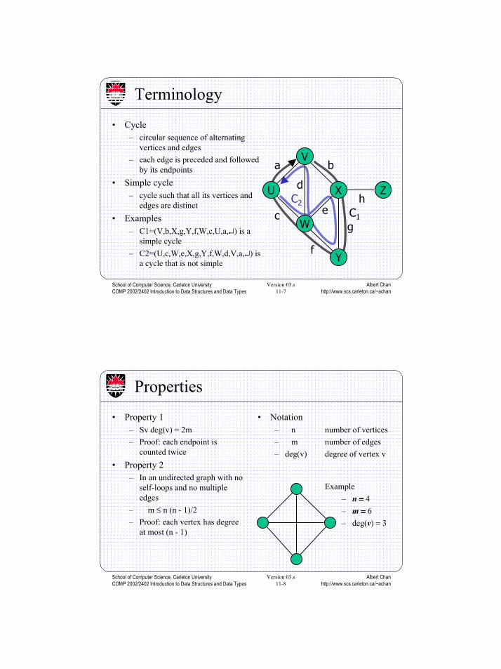
Version 03.s11-7

C1

XU

V

W

Z

Y

a

c

b

e

d

f

g

hC2

Terminology

• Cycle– circular sequence of alternating

vertices and edges– each edge is preceded and followed

by its endpoints• Simple cycle

– cycle such that all its vertices andedges are distinct

• Examples– C1=(V,b,X,g,Y,f,W,c,U,a,↵) is a

simple cycle– C2=(U,c,W,e,X,g,Y,f,W,d,V,a,↵) is

a cycle that is not simple



Version 03.s11-8

Example– n = = = = 4– m = = = = 6– deg(v) = 3

Properties

• Notation– n number of vertices– m number of edges– deg(v) degree of vertex v

• Property 1– Sv deg(v) = 2m– Proof: each endpoint is

counted twice• Property 2

– In an undirected graph with noself-loops and no multipleedges

– m ≤ n (n - 1)/2– Proof: each vertex has degree

at most (n - 1)



Version 03.s11-9

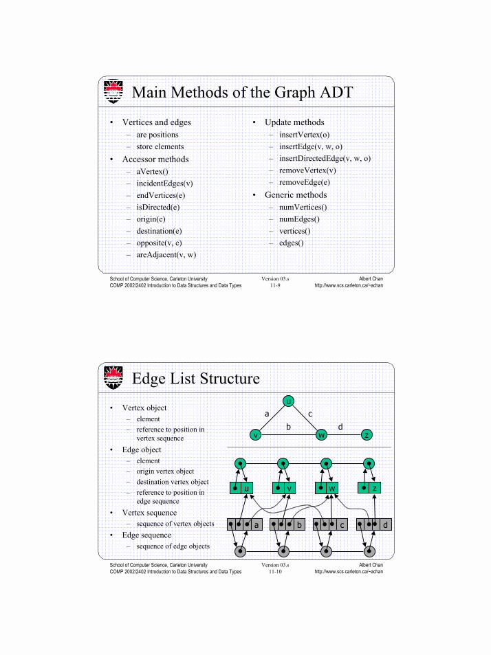
Main Methods of the Graph ADT

• Vertices and edges– are positions– store elements

• Accessor methods– aVertex()– incidentEdges(v)– endVertices(e)– isDirected(e)– origin(e)– destination(e)– opposite(v, e)– areAdjacent(v, w)

• Update methods– insertVertex(o)– insertEdge(v, w, o)– insertDirectedEdge(v, w, o)– removeVertex(v)– removeEdge(e)

• Generic methods– numVertices()– numEdges()– vertices()– edges()



Version 03.s11-10

v

u

w

a c

b

a

zd

u v w z

b c d

Edge List Structure• Vertex object

– element– reference to position in

vertex sequence• Edge object

– element– origin vertex object– destination vertex object– reference to position in

edge sequence• Vertex sequence

– sequence of vertex objects• Edge sequence

– sequence of edge objects



Version 03.s11-11

u

v

wa b

a

u v w

b

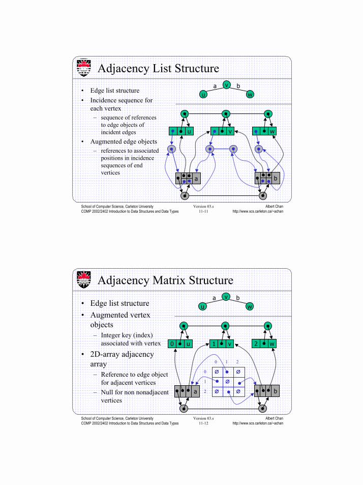
Adjacency List Structure

• Edge list structure• Incidence sequence for

each vertex– sequence of references

to edge objects ofincident edges

• Augmented edge objects– references to associated

positions in incidencesequences of endvertices



Version 03.s11-12

u

v

wa b

2

1

0

210

∅∅∅∅∅∅∅∅

∅∅∅∅

∅∅∅∅∅∅∅∅

a

u v w0 1 2

b

Adjacency Matrix Structure

• Edge list structure• Augmented vertex

objects– Integer key (index)

associated with vertex

• 2D-array adjacencyarray– Reference to edge object

for adjacent vertices– Null for non nonadjacent

vertices



Version 03.s11-13

Performance

n2n + mn + mSpace

n2deg(v)mremoveVertex(v)

111insertEdge(v, w, o)

n211insertVertex(o)

111removeEdge(e)

1min(deg(v), deg(w))mareAdjacent (v, w)

ndeg(v)mincidentEdges(v)

AdjacencyMatrix

AdjacencyList

EdgeList

• n vertices• m edges• no parallel edges• no self-loops



Version 03.s11-14

Subgraph

Spanning subgraph

Subgraphs

• A subgraph S of a graph Gis a graph such that– The edges of S are a subset

of the edges of G– The edges of S are a subset

of the edges of G

• A spanning subgraph of Gis a subgraph that containsall the vertices of G



Version 03.s11-15

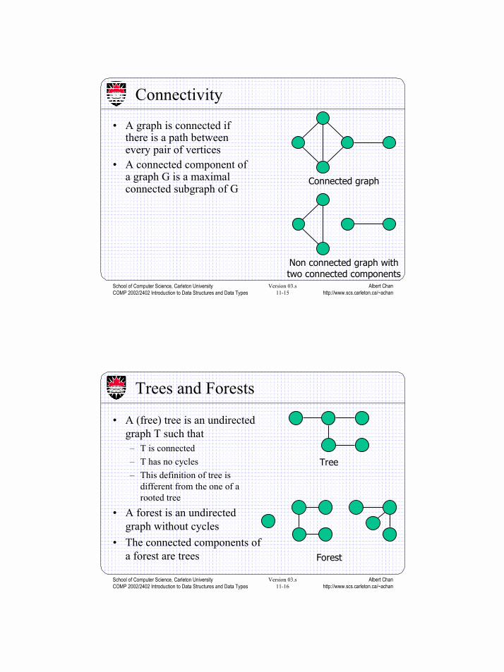
Connectivity

• A graph is connected ifthere is a path betweenevery pair of vertices

• A connected component ofa graph G is a maximalconnected subgraph of G

Connected graph

Non connected graph withtwo connected components



Version 03.s11-16

Tree

Forest

Trees and Forests

• A (free) tree is an undirectedgraph T such that– T is connected– T has no cycles– This definition of tree is

different from the one of arooted tree

• A forest is an undirectedgraph without cycles

• The connected components ofa forest are trees



Version 03.s11-17

Graph

Spanning tree

Spanning Trees and Forests

• A spanning tree of a connectedgraph is a spanning subgraphthat is a tree

• A spanning tree is not uniqueunless the graph is a tree

• Spanning trees have applicationsto the design of communicationnetworks

• A spanning forest of a graph is aspanning subgraph that is aforest



Version 03.s11-18

Depth-First Search

• Depth-first search (DFS) is ageneral technique for traversinga graph

• A DFS traversal of a graph G– Visits all the vertices and

edges of G– Determines whether G is

connected– Computes the connected

components of G– Computes a spanning forest of

G

• DFS on a graph with n verticesand m edges takes O(n + m )time

• DFS can be further extended tosolve other graph problems

– Find and report a path betweentwo given vertices

– Find a cycle in the graph• Depth-first search is to graphs

what Euler tour is to binarytrees



Version 03.s11-19

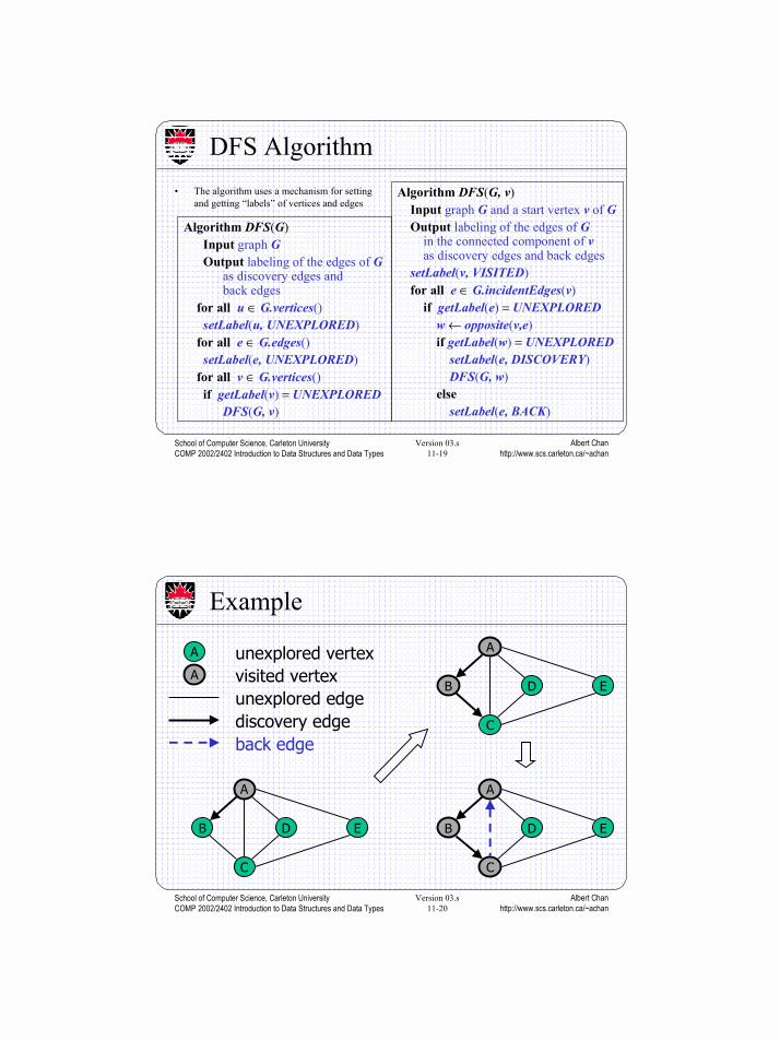
Algorithm DFS(G, v)Input graph G and a start vertex v of GOutput labeling of the edges of G

in the connected component of vas discovery edges and back edges

setLabel(v, VISITED)for all e ∈ G.incidentEdges(v)

if getLabel(e) = UNEXPLOREDw ← opposite(v,e)if getLabel(w) = UNEXPLORED

setLabel(e, DISCOVERY)DFS(G, w)

elsesetLabel(e, BACK)

Algorithm DFS(G)Input graph GOutput labeling of the edges of G

as discovery edges andback edges

for all u ∈ G.vertices()setLabel(u, UNEXPLORED)

for all e ∈ G.edges()setLabel(e, UNEXPLORED)

for all v ∈ G.vertices()if getLabel(v) = UNEXPLORED

DFS(G, v)

DFS Algorithm• The algorithm uses a mechanism for setting

and getting “labels” of vertices and edges



Version 03.s11-20

Example

DB

A

C

E

DB

A

C

E

DB

A

C

E

discovery edgeback edge

A visited vertexA unexplored vertex

unexplored edge



Version 03.s11-21

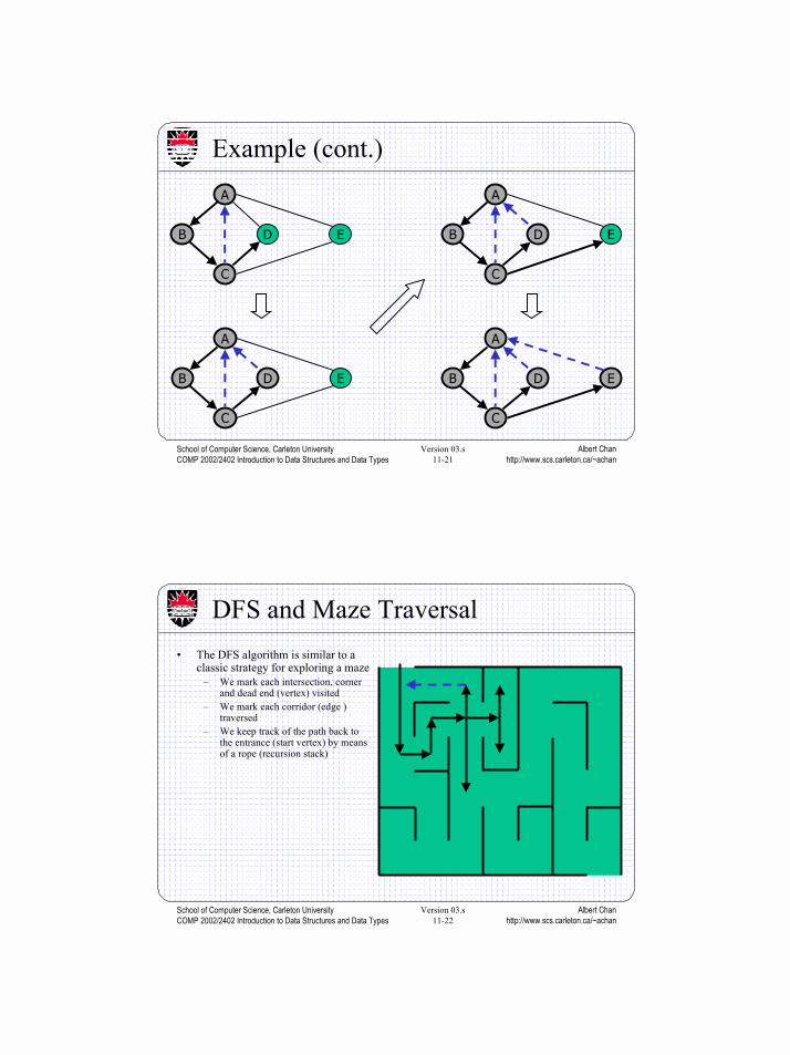
Example (cont.)

DB

A

C

E

DB

A

C

E

DB

A

C

E

DB

A

C

E



Version 03.s11-22

DFS and Maze Traversal• The DFS algorithm is similar to a

classic strategy for exploring a maze– We mark each intersection, corner

and dead end (vertex) visited– We mark each corridor (edge )

traversed– We keep track of the path back to

the entrance (start vertex) by meansof a rope (recursion stack)



Version 03.s11-23

DB

A

C

E

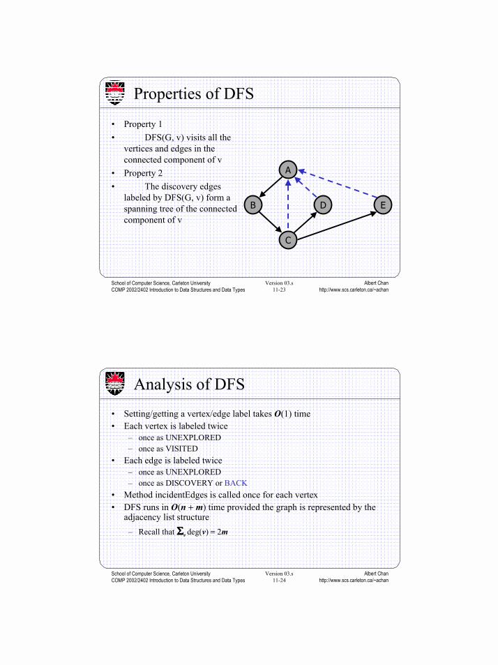
Properties of DFS

• Property 1• DFS(G, v) visits all the

vertices and edges in theconnected component of v

• Property 2• The discovery edges

labeled by DFS(G, v) form aspanning tree of the connectedcomponent of v



Version 03.s11-24

Analysis of DFS• Setting/getting a vertex/edge label takes O(1) time• Each vertex is labeled twice

– once as UNEXPLORED– once as VISITED

• Each edge is labeled twice– once as UNEXPLORED– once as DISCOVERY or BACK

• Method incidentEdges is called once for each vertex• DFS runs in O(n + m) time provided the graph is represented by the

adjacency list structure– Recall that ΣΣΣΣv deg(v) = 2m



Version 03.s11-25

Algorithm pathDFS(G, v, z)setLabel(v, VISITED)S.push(v)if v = z

return S.elements()for all e ∈ G.incidentEdges(v)

if getLabel(e) = UNEXPLOREDw ← opposite(v,e)if getLabel(w) = UNEXPLORED

setLabel(e, DISCOVERY)S.push(e)pathDFS(G, w, z)S.pop(e)

else setLabel(e, BACK)

S.pop(v)

Path Finding

• We can specialize the DFSalgorithm to find a path betweentwo given vertices u and z usingthe template method pattern

• We call DFS(G, u) with u as thestart vertex

• We use a stack S to keep trackof the path between the startvertex and the current vertex

• As soon as destination vertex zis encountered, we return thepath as the contents of the stack



Version 03.s11-26

Cycle Finding

• We can specialize the DFSalgorithm to find a simple cycleusing the template methodpattern

• We use a stack S to keep trackof the path between the startvertex and the current vertex

• As soon as a back edge (v, w)is encountered, we return thecycle as the portion of the stackfrom the top to vertex w

Algorithm cycleDFS(G, v, z)setLabel(v, VISITED)S.push(v)for all e ∈ G.incidentEdges(v)

if getLabel(e) = UNEXPLOREDw ← opposite(v,e)S.push(e)if getLabel(w) = UNEXPLORED

setLabel(e, DISCOVERY)pathDFS(G, w, z)S.pop(e)

elseT ← new empty stackrepeat

o ← S.pop()T.push(o)

until o = wreturn T.elements()

S.pop(v)



Version 03.s11-27

Breadth-First Search

• Breadth-first search (BFS) is ageneral technique for traversinga graph

• A BFS traversal of a graph G– Visits all the vertices and

edges of G– Determines whether G is

connected– Computes the connected

components of G– Computes a spanning forest of

G

• BFS on a graph with n verticesand m edges takes O(n + m )time

• BFS can be further extended tosolve other graph problems

– Find and report a path with theminimum number of edgesbetween two given vertices

– Find a simple cycle, if there isone



Version 03.s11-28

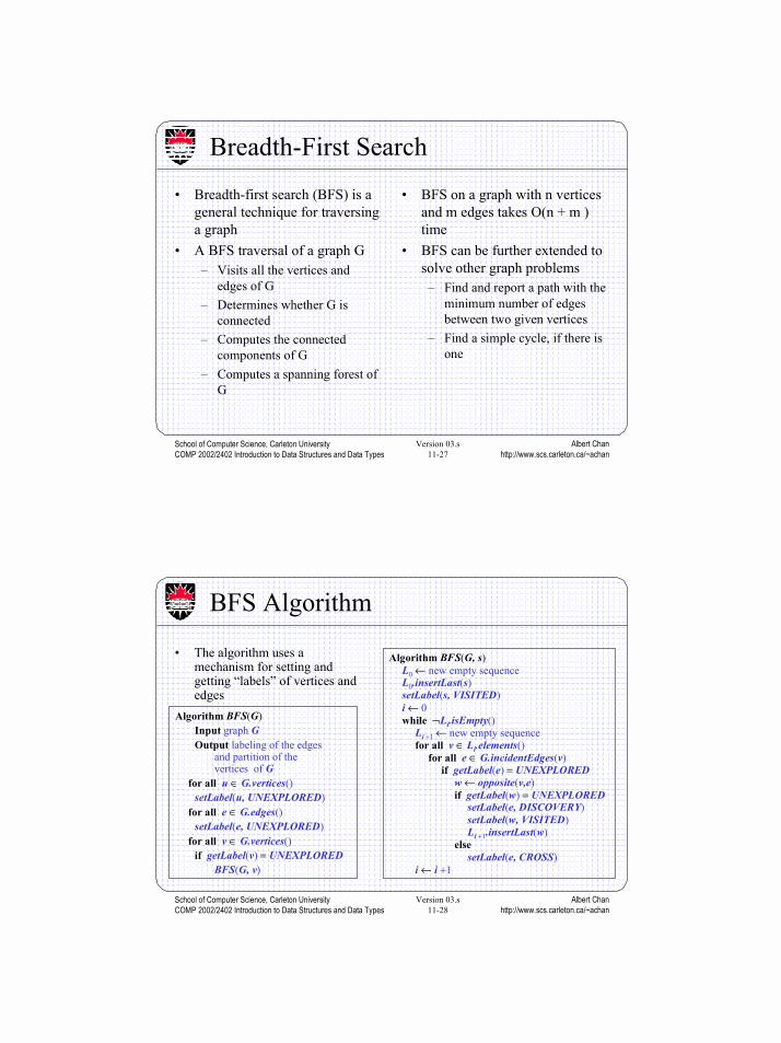
BFS Algorithm

• The algorithm uses amechanism for setting andgetting “labels” of vertices andedges

Algorithm BFS(G, s)L0 ← new empty sequenceL0.insertLast(s)setLabel(s, VISITED)i ← 0while ¬Li.isEmpty()

Li +1 ← new empty sequencefor all v ∈ Li.elements()

for all e ∈ G.incidentEdges(v)if getLabel(e) = UNEXPLORED

w ← opposite(v,e)if getLabel(w) = UNEXPLORED

setLabel(e, DISCOVERY)setLabel(w, VISITED)Li +1.insertLast(w)

elsesetLabel(e, CROSS)

i ← i +1

Algorithm BFS(G)Input graph GOutput labeling of the edges

and partition of thevertices of G

for all u ∈ G.vertices()setLabel(u, UNEXPLORED)

for all e ∈ G.edges()setLabel(e, UNEXPLORED)

for all v ∈ G.vertices()if getLabel(v) = UNEXPLORED

BFS(G, v)



Version 03.s11-29

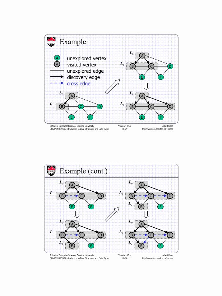
Example

CB

A

E

D

discovery edgecross edge

A visited vertexA unexplored vertex

unexplored edge

L0

L1

F

CB

A

E

D

L0

L1

F

CB

A

E

D

L0

L1

F



Version 03.s11-30

Example (cont.)

CB

A

E

D

L0

L1

F

CB

A

E

D

L0

L1

FL2

CB

A

E

D

L0

L1

FL2

CB

A

E

D

L0

L1

FL2



Version 03.s11-31

Example (cont.)

CB

A

E

D

L0

L1

FL2

CB

A

E

D

L0

L1

FL2

CB

A

E

D

L0

L1

FL2



Version 03.s11-32

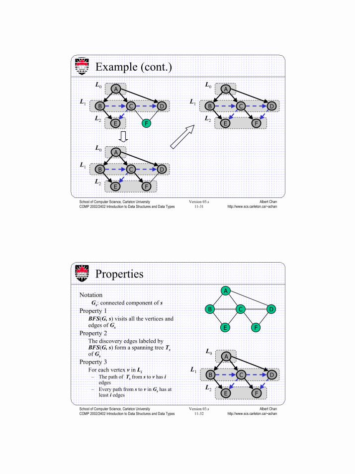
PropertiesNotation

Gs: connected component of sProperty 1

BFS(G, s) visits all the vertices andedges of Gs

Property 2The discovery edges labeled byBFS(G, s) form a spanning tree Tsof Gs

Property 3For each vertex v in Li

– The path of Ts from s to v has iedges

– Every path from s to v in Gs has atleast i edges

CB

A

E

D

L0

L1

FL2

CB

A

E

D

F



Version 03.s11-33

Analysis• Setting/getting a vertex/edge label takes O(1) time• Each vertex is labeled twice

– once as UNEXPLORED– once as VISITED

• Each edge is labeled twice– once as UNEXPLORED– once as DISCOVERY or CROSS

• Each vertex is inserted once into a sequence Li• Method incidentEdges is called once for each vertex• BFS runs in O(n + m) time provided the graph is represented by the

adjacency list structure– Recall that ΣΣΣΣv deg(v) = 2m



Version 03.s11-34

Applications

• Using the template method pattern, we can specialize theBFS traversal of a graph G to solve the following problemsin O(n + m) time– Compute the connected components of G– Compute a spanning forest of G– Find a simple cycle in G, or report that G is a forest– Given two vertices of G, find a path in G between them with the

minimum number of edges, or report that no such path exists



Version 03.s11-35

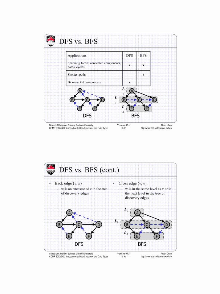
DFS vs. BFS

CB

A

E

D

L0

L1

FL2

CB

A

E

D

F

DFS BFS

√√√√Biconnected components

√√√√Shortest paths

√√√√√√√√Spanning forest, connected components,paths, cycles

BFSDFSApplications



Version 03.s11-36

CB

A

E

D

L0

L1

FL2

CB

A

E

D

F

DFS BFS

DFS vs. BFS (cont.)

• Back edge (v,w)– w is an ancestor of v in the tree

of discovery edges

• Cross edge (v,w)– w is in the same level as v or in

the next level in the tree ofdiscovery edges



Version 03.s11-37

Separation Edges and Vertices• Definitions

– Let G be a connected graph– A separation edge of G is an edge whose removal disconnects G– A separation vertex of G is a vertex whose removal disconnects G

• Applications– Separation edges and vertices represent single points of failure in a network and are

critical to the operation of the network• Example

– DFW, LGA and LAX are separation vertices– (DFW,LAX) is a separation edge

ORD PVD

MIADFW

SFO

LAX

LGA

HNL



Version 03.s11-38

ORDPVD

MIADFW

SFO

LAX

LGAHNL

Biconnected Graph

• Equivalent definitions of a biconnected graph G– Graph G has no separation edges and no separation vertices– For any two vertices u and v of G, there are two disjoint simple

paths between u and v (i.e., two simple paths between u and v thatshare no other vertices or edges)

– For any two vertices u and v of G, there is a simple cyclecontaining u and v

• Example



Version 03.s11-39

ORD PVD

MIADFW

SFO

LAX

LGA

HNLRDU

Biconnected Components• Biconnected component of a graph G

– A maximal biconnected subgraph of G, or– A subgraph consisting of a separation edge of G and its end vertices

• Interaction of biconnected components– An edge belongs to exactly one biconnected component– A nonseparation vertex belongs to exactly one biconnected component– A separation vertex belongs to two or more biconnected components

• Example of a graph with four biconnected components



Version 03.s11-40

Equivalence Classes• Given a set S, a relation R on S is a set of ordered pairs of elements of S, i.e., R is a

subset of S×S• An equivalence relation R on S satisfies the following properties

– Reflexive: (x,x) ∈ R– Symmetric: (x,y) ∈ R ⇒ (y,x) ∈ R– Transitive: (x,y) ∈ R ∧ (y,z) ∈ R ⇒ (x,z) ∈ R

• An equivalence relation R on S induces a partition of the elements of S into equivalenceclasses

• Example (connectivity relation among the vertices of a graph):– Let V be the set of vertices of a graph G– Define the relation

C = {(v,w) ∈ V×V such that G has a path from v to w}– Relation C is an equivalence relation– The equivalence classes of relation C are the vertices in each connected component of graph G



Version 03.s11-41

ab

g

cj

de

f

i

Equivalence classes of linked edges:{a} {b, c, d, e, f} {g, i, j}

ab

g

cj

de

f

i

Link Relation• Edges e and f of connected graph

G are linked if– e = f, or– G has a simple cycle containing

e and f• Theorem:The link relation on the

edges of a graph is anequivalence relation

– Proof Sketch:– The reflexive and symmetric

properties follow from thedefinition

– For the transitive property,consider two simple cyclessharing an edge



Version 03.s11-42

Link Components• The link components of a connected graph G are the equivalence classes of

edges with respect to the link relation• A biconnected component of G is the subgraph of G induced by an

equivalence class of linked edges• A separation edge is a single-element equivalence class of linked edges• A separation vertex has incident edges in at least two distinct equivalence

classes of linked edge

ORD PVD

MIADFW

SFO

LAX

LGA

HNLRDU



Version 03.s11-43

a

bg

cj

d

e

f

i

Auxiliary graph B

DFS on graph G

a

db

c

eh i

jf

h

g

i

Auxiliary Graph• Auxiliary graph B for a connected

graph G– Associated with a DFS traversal of

G– The vertices of B are the edges of G– For each back edge e of G, B has

edges (e,f1), (e,f2) , …, (e,fk),where f1, f2, …, fk are thediscovery edges of G that form asimple cycle with e

– Its connected componentscorrespond to the the linkcomponents of G



Version 03.s11-44

Auxiliary graph BDFS on graph G

Auxiliary Graph (cont.)

• In the worst case, the number of edges of the auxiliarygraph is proportional to nm



Version 03.s11-45

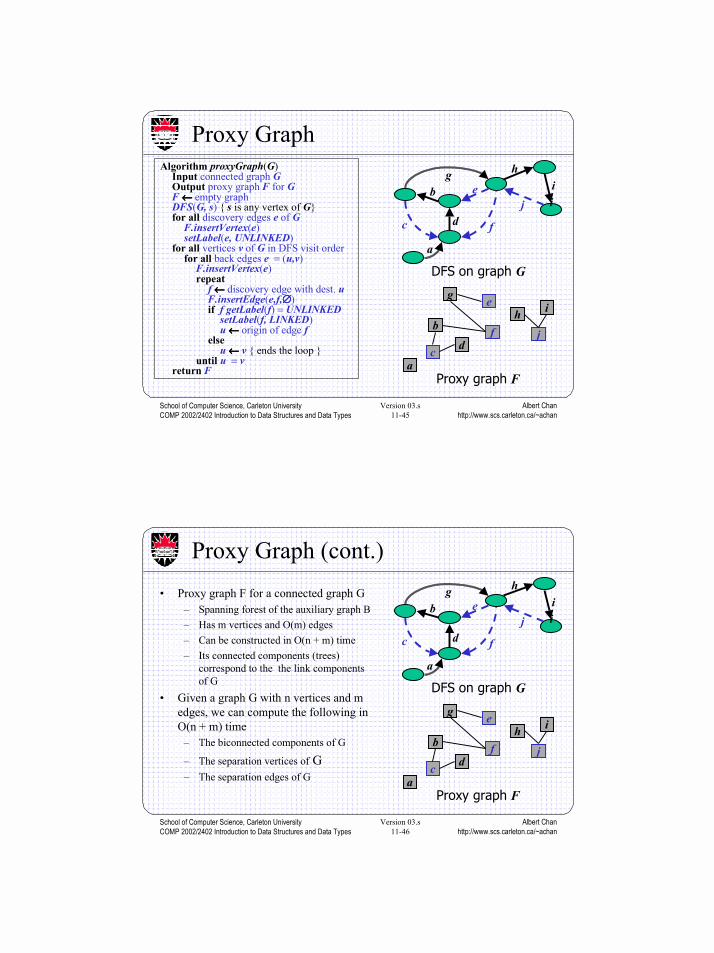
Proxy GraphAlgorithm proxyGraph(G)

Input connected graph GOutput proxy graph F for GF ←←←← empty graphDFS(G, s) { s is any vertex of G}for all discovery edges e of G

F.insertVertex(e)setLabel(e, UNLINKED)

for all vertices v of G in DFS visit orderfor all back edges e = (u,v)

F.insertVertex(e)repeat

f ←←←← discovery edge with dest. uF.insertEdge(e,f,∅∅∅∅)if f getLabel(f) = UNLINKED

setLabel(f, LINKED)u ←←←← origin of edge f

elseu ←←←← v { ends the loop }

until u = vreturn F

a

bg

cj

d

e

f

i

Proxy graph F

DFS on graph G

a

db

c

eh i

jf

h

g

i



Version 03.s11-46

a

bg

cj

d

e

f

i

Proxy graph F

DFS on graph G

a

db

c

eh i

jf

h

g

i

Proxy Graph (cont.)• Proxy graph F for a connected graph G

– Spanning forest of the auxiliary graph B– Has m vertices and O(m) edges– Can be constructed in O(n + m) time– Its connected components (trees)

correspond to the the link componentsof G

• Given a graph G with n vertices and medges, we can compute the following inO(n + m) time

– The biconnected components of G

– The separation vertices of G– The separation edges of G



Version 03.s11-47

A

C

E

B

D

Digraphs

• A digraph is a directed graph whose edges are all directed• Applications

– one-way streets– flights– task scheduling



Version 03.s11-48

A

C

E

B

D

Directed DFS

• We can specialize the traversalalgorithms (DFS and BFS) todigraphs by traversing edgesonly along their direction

• In the directed DFS algorithm,we have four types of edges

– discovery edges– back edges– forward edges– cross edges

• A directed DFS starting a avertex s determines the verticesreachable from s



Version 03.s11-49

B

A

D

C

E

B

A

D

C

E

G

G*

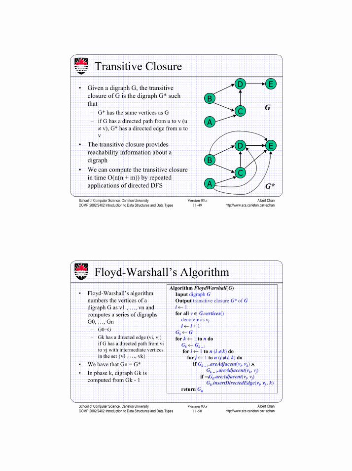
Transitive Closure

• Given a digraph G, the transitiveclosure of G is the digraph G* suchthat

– G* has the same vertices as G– if G has a directed path from u to v (u

≠ v), G* has a directed edge from u tov

• The transitive closure providesreachability information about adigraph

• We can compute the transitive closurein time O(n(n + m)) by repeatedapplications of directed DFS



Version 03.s11-50

Algorithm FloydWarshall(G)Input digraph GOutput transitive closure G* of Gi ← 1for all v ∈ G.vertices()

denote v as vii ← i + 1

G0 ← Gfor k ← 1 to n do

Gk ← Gk −−−− 1 for i ← 1 to n (i ≠≠≠≠ k) do

for j ← 1 to n (j ≠≠≠≠ i, k) doif Gk −−−− 1.areAdjacent(vi, vk) ∧∧∧∧

Gk −−−− 1.areAdjacent(vk, vj) if ¬¬¬¬Gk.areAdjacent(vi, vj)

Gk.insertDirectedEdge(vi, vj , k)return Gn

Floyd-Warshall’s Algorithm• Floyd-Warshall’s algorithm

numbers the vertices of adigraph G as v1 , …, vn andcomputes a series of digraphsG0, …, Gn

– G0=G– Gk has a directed edge (vi, vj)

if G has a directed path from vito vj with intermediate verticesin the set {v1 , …, vk}

• We have that Gn = G*• In phase k, digraph Gk is

computed from Gk - 1



Version 03.s11-51

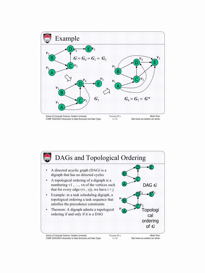
Examplev4

v5

B

A

D

C

E

B

A

D

C

E

B

A

D

C

EG = G0 = G1 = G2

G3 G4 = G5 = G*

v1

v2

v3

v4v5

v1

v2

v3

v1

v2

v3

v4v5



Version 03.s11-52

B

A

D

C

E

DAG G

B

A

D

C

E

Topological

orderingof G

v1

v2

v3

v4 v5

DAGs and Topological Ordering

• A directed acyclic graph (DAG) is adigraph that has no directed cycles

• A topological ordering of a digraph is anumbering v1 , …, vn of the vertices suchthat for every edge (vi , vj), we have i < j

• Example: in a task scheduling digraph, atopological ordering a task sequence thatsatisfies the precedence constraints

• Theorem: A digraph admits a topologicalordering if and only if it is a DAG



Version 03.s11-53

Minimum Spanning TreeSpanning subgraph

– Subgraph of a graph Gcontaining all the vertices ofG

Spanning tree– Spanning subgraph that is

itself a (free) treeMinimum spanning tree (MST)

– Spanning tree of a weightedgraph with minimum totaledge weight

• Applications– Communications networks– Transportation networks

ORD

PIT

ATL

STL

DEN

DFW

DCA

101

9

8

6

3

25

7

4



Version 03.s11-54

84

2 36

7

7

9

8e

Cf

84

2 36

7

7

9

8

C

e

f

Replacing f with e yieldsa better spanning tree

Cycle Property

• Cycle Property:– Let T be a minimum spanning

tree of a weighted graph G– Let e be an edge of G that is not

in T and C let be the cycleformed by e with T

– For every edge f of C, weight(f)≤ weight(e)

– Proof:– By contradiction– If weight(f) > weight(e) we can

get a spanning tree of smallerweight by replacing e with f



Version 03.s11-55

U V

74

2 85

7

3

9

8 e

f

74

2 85

7

3

9

8 e

f

Replacing f with e yieldsanother MST

U V

Partition Property• Partition Property:

– Consider a partition of the vertices of Ginto subsets U and V

– Let e be an edge of minimum weightacross the partition

– There is a minimum spanning tree of Gcontaining edge e

– Proof:– Let T be an MST of G– If T does not contain e, consider the

cycle C formed by e with T and let f bean edge of C across the partition

– By the cycle property,weight(f) ≤ weight(e)

– Thus, weight(f) = weight(e)– We obtain another MST by replacing f

with e



Version 03.s11-56

Prim-Jarnik’s Algorithm

• Prim-Jarnik’s algorithm for computing an MST is similar to Dijkstra’salgorithm

• We assume that the graph is connected• We pick an arbitrary vertex s and we grow the MST as a cloud of

vertices, starting from s• We store with each vertex v a label d(v) representing the smallest

weight of an edge connecting v to a vertex in the cloud• At each step

– We add to the cloud the vertex u outside the cloud with the smallestdistance label

– We update the labels of the vertices adjacent to u



Version 03.s11-57

Algorithm PrimJarnikMST(G)Q ← new heap-based priority queues ← a vertex of Gfor all v ∈ G.vertices()

if v = ssetDistance(v, 0)

elsesetDistance(v, ∞∞∞∞)

setParent(v, ∅∅∅∅)l ← Q.insert(getDistance(v), v)setLocator(v,l)

while ¬Q.isEmpty()u ← Q.removeMin()for all e ∈ G.incidentEdges(u)

z ← G.opposite(u,e)r ← weight(e)if r < getDistance(z)

setDistance(z,r)setParent(z,e)

Q.replaceKey(getLocator(z),r)

Prim-Jarnik’s Algorithm (cont.)

• A priority queue stores thevertices outside the cloud

– Key: distance– Element: vertex

• Locator-based methods– insert(k,e) returns a locator– replaceKey(l,k) changes the

key of an item• We store three labels with

each vertex:– Distance– Parent edge in MST– Locator in priority queue



Version 03.s11-58

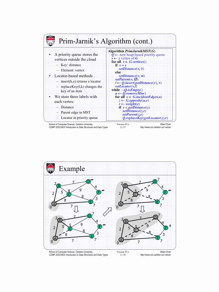
Example

BD

C

A

F

E

74

28

5

7

3

9

8

0 7

2

8 ∞∞∞∞

∞∞∞∞

BD

C

A

F

E

74

28

5

7

3

9

8

0 7

2

5 ∞∞∞∞

7

BD

C

A

F

E

74

28

5

7

3

9

8

0 7

2

5 ∞∞∞∞

7

BD

C

A

F

E

74

28

5

7

3

9

8

0 7

2

5 4

7



Version 03.s11-59

Example (contd.)

BD

C

A

F

E

74

28

5

7

3

9

8

0 3

2

5 4

7

BD

C

A

F

E

74

28

5

7

3

9

8

0 3

2

5 4

7



Version 03.s11-60

Analysis• Graph operations

– Method incidentEdges is called once for each vertex• Label operations

– We set/get the distance, parent and locator labels of vertex z O(deg(z)) times– Setting/getting a label takes O(1) time

• Priority queue operations– Each vertex is inserted once into and removed once from the priority queue, where

each insertion or removal takes O(log n) time– The key of a vertex w in the priority queue is modified at most deg(w) times, where

each key change takes O(log n) time• Prim-Jarnik’s algorithm runs in O((n + m) log n) time provided the graph is

represented by the adjacency list structure– Recall that Sv deg(v) = 2m

• The running time is O(m log n) since the graph is connected



Version 03.s11-61

Dijkstra vs. Prim-Jarnik

Algorithm PrimJarnikMST(G)Q ← new heap-based priority queues ← a vertex of Gfor all v ∈ G.vertices()



setParent(v, ∅∅∅∅)l ← Q.insert(getDistance(v), v)setLocator(v,l)


z ← G.opposite(u,e)r ← weight(e)if r < getDistance(z)



Algorithm DijkstraShortestPaths(G, s)Q ← new heap-based priority queue

for all v ∈ G.vertices()if v = s

setDistance(v, 0)else

setDistance(v, ∞∞∞∞) setParent(v, ∅∅∅∅)

l ← Q.insert(getDistance(v), v)setLocator(v,l)


z ← G.opposite(u,e)r ← getDistance(u) + weight(e)if r < getDistance(z)





Version 03.s11-62

Algorithm KruskalMST(G)for each vertex V in G do

define a Cloud(v) of ! {v}let Q be a priority queue.Insert all edges into Q using their weights as the

keyT ! ∅∅∅∅while T has fewer than n-1 edges do

edge e = T.removeMin()Let u, v be the endpoints of eif Cloud(v) ≠≠≠≠ Cloud(u) then

Add edge e to TMerge Cloud(v) and Cloud(u)

return T

Kruskal’s Algorithm

• A priority queue storesthe edges outside thecloud

– Key: weight– Element: edge

• At the end of thealgorithm

– We are left with onecloud thatencompasses theMST

– A tree T which is ourMST



Version 03.s11-63

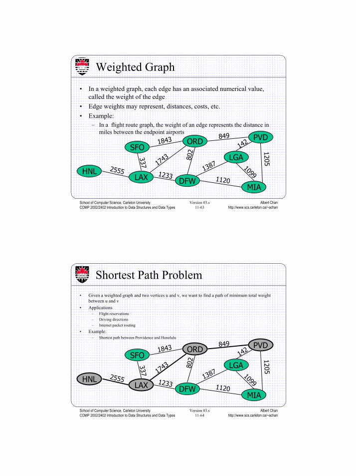
ORD PVD

MIADFW

SFO

LAX

LGA

HNL

849

802

13871743

1843

10991120

1233

337

2555

142

1205

Weighted Graph

• In a weighted graph, each edge has an associated numerical value,called the weight of the edge

• Edge weights may represent, distances, costs, etc.• Example:

– In a flight route graph, the weight of an edge represents the distance inmiles between the endpoint airports



Version 03.s11-64

ORD PVD

MIADFW

SFO

LAX

LGA

HNL

849

802

13871743

1843

10991120

1233

337

2555

142

1205

Shortest Path Problem• Given a weighted graph and two vertices u and v, we want to find a path of minimum total weight

between u and v• Applications

– Flight reservations– Driving directions– Internet packet routing

• Example:– Shortest path between Providence and Honolulu



Version 03.s11-65

ORD PVD

MIADFW

SFO

LAX

LGA

HNL

849

802

13871743

1843

10991120

1233

337

2555

142

1205

Shortest Path Properties

• Property 1: A subpath of a shortest path is itself a shortest path• Property 2: There is a tree of shortest paths from a start vertex to all the

other vertices• Example: Tree of shortest paths from Providence



Version 03.s11-66

Dijkstra’s Algorithm

• The distance of a vertex v froma vertex s is the length of ashortest path between s and v

• Dijkstra’s algorithm computesthe distances of all the verticesfrom a given start vertex s

• Assumptions:– the graph is connected– the edges are undirected– the edge weights are

nonnegative

• We grow a “cloud” of vertices,beginning with s and eventuallycovering all the vertices

• We store with each vertex v alabel d(v) representing thedistance of v from s in thesubgraph consisting of thecloud and its adjacent vertices

• At each step– We add to the cloud the vertex

u outside the cloud with thesmallest distance label

– We update the labels of thevertices adjacent to u



Version 03.s11-67

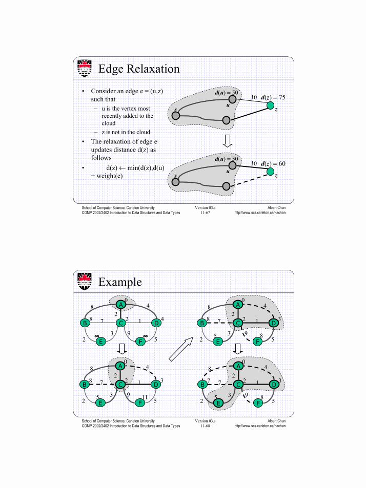
d(z) = 75

d(u) = 5010

zsu

d(z) = 60

d(u) = 5010

zsu

Edge Relaxation

• Consider an edge e = (u,z)such that

– u is the vertex mostrecently added to thecloud

– z is not in the cloud• The relaxation of edge e

updates distance d(z) asfollows

• d(z) ← min(d(z),d(u)+ weight(e)



Version 03.s11-68

Example

CB

A

E

D

F

0

428

∞∞∞∞ ∞∞∞∞

48

7 1

2 5

2

3 9

CB

A

E

D

F

0

328

5 11

48

7 1

2 5

2

3 9

CB

A

E

D

F

0

328

5 8

48

7 1

2 5

2

3 9

CB

A

E

D

F

0

327

5 8

48

7 1

2 5

2

3 9



Version 03.s11-69

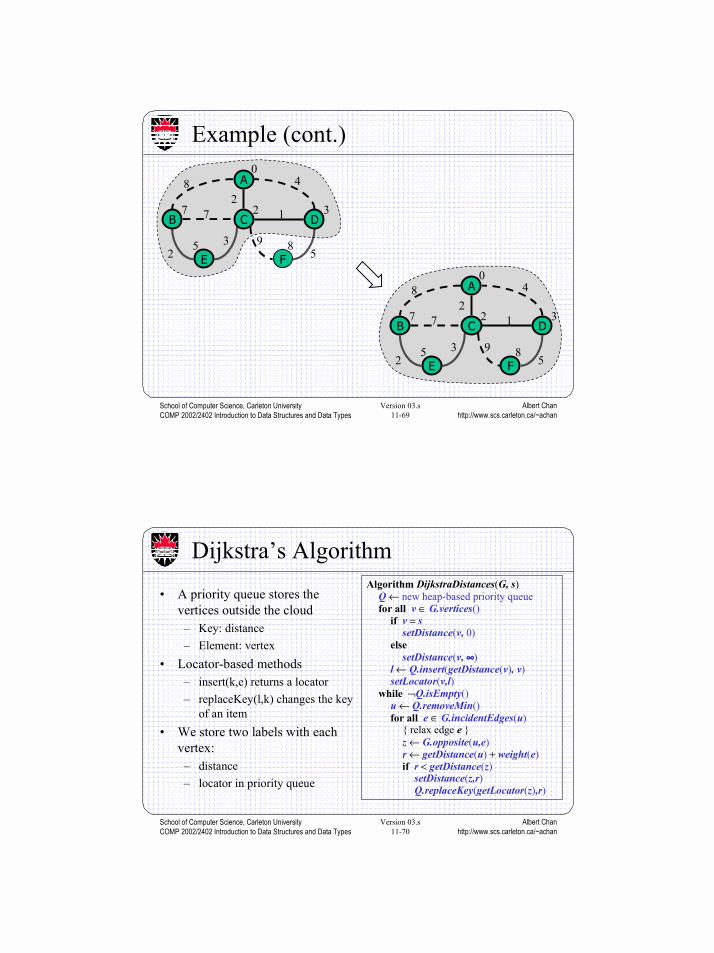
Example (cont.)

CB

A

E

D

F

0

327

5 8

48

7 1

2 5

2

3 9

CB

A

E

D

F

0

327

5 8

48

7 1

2 5

2

3 9



Version 03.s11-70

Algorithm DijkstraDistances(G, s)Q ← new heap-based priority queuefor all v ∈ G.vertices()



l ← Q.insert(getDistance(v), v)setLocator(v,l)


{ relax edge e }z ← G.opposite(u,e)r ← getDistance(u) + weight(e)if r < getDistance(z)

setDistance(z,r) Q.replaceKey(getLocator(z),r)

Dijkstra’s Algorithm

• A priority queue stores thevertices outside the cloud

– Key: distance– Element: vertex

• Locator-based methods– insert(k,e) returns a locator– replaceKey(l,k) changes the key

of an item• We store two labels with each

vertex:– distance– locator in priority queue



Version 03.s11-71

Analysis• Graph operations

– Method incidentEdges is called once for each vertex• Label operations

– We set/get the distance and locator labels of vertex z O(deg(z)) times– Setting/getting a label takes O(1) time

• Priority queue operations– Each vertex is inserted once into and removed once from the priority queue, where

each insertion or removal takes O(log n) time– The key of a vertex in the priority queue is modified at most deg(w) times, where

each key change takes O(log n) time• Dijkstra’s algorithm runs in O((n + m) log n) time provided the graph is

represented by the adjacency list structure– Recall that ΣΣΣΣv deg(v) = 2m

• The running time can also be expressed as O(m log n) since the graph isconnected

Graphs - Carleton University

Documents

Graphs - Carleton University