1
de l'Document de travail
GOVERNMENTS UNDER INFLUENCE :
COUNTRY INTERACTIONS IN DISCRETIONARY FISCAL POLICY
N° 2010-25
OCTOBRE 2010
Aurélie Cassette EQUIPPE-Université de Lille
Jérôme Creel ESCP Europe and OFCE
Etienne Farvaque EQUIPPE-Université de Lille
Sonia Paty
CREM-Université de CAEN and CNRS
OFCE - Centre de recherche en économie de Sciences Po 69, quai d’Orsay - 75340 Paris Cedex 07 Tél/ 01 44 18 54 00 - Fax/ 01 45 56 06 15
www.ofce.sciences-po.fr

2
Governments under influence: Country interactions in discretionary fiscal policy
Aurélie Cassette EQUIPPE-Universités de Lille, Faculté des sciences économiques et sociales –Université
de Lille 1, 59655 Villeneuve d’Ascq Cedex (France) [email protected]
Jérôme Creel
ESCP Europe and OFCE / Sciences Po (Economic Research Department), 69, quai d'Orsay, F-75340 Paris Cedex 07 (France)
Etienne Farvaque EQUIPPE-Universités de Lille, Faculté des sciences économiques et sociales –Université
de Lille 1, 59655 Villeneuve d’Ascq Cedex (France) [email protected]
Sonia Paty
CREM – Université de Caen and CNRS (France) and EQUIPPE-Universités de Lille, Faculté des sciences économiques et sociales –Université de Lille 1, 59655 Villeneuve
d’Ascq Cedex (France). Tel : + 33 3 20 33 72 10 [email protected]
Abstract We investigate the interactions between countries of the discretionary component of national fiscal policies (i.e. the cyclically- and interest-adjusted part of fiscal policy), therefore observing and investigating the part of public spending and tax receipts on which governments keep full discretion. Our sample covers 18 OECD countries, during the 1974-2008 period. First, we build a measure of such discretionary fiscal policy, considered as the residual component of a VAR model, and compute the measure for the full sample. Drawing on this new dataset, the second step provides estimates of discretionary fiscal policy interactions between countries of the sample. Our results highlight the existence of interactions between neighboring countries' public decisions, where neighborhood is defined by economic leadership as well as geography. We also find evidence of an opportunistic behavior of OECD countries' governments for the discretionary public spending. Finally, the disciplining device of the European Union fiscal framework is shown to be ineffective.
Keywords: Fiscal policy; discretion; interactions; VAR; spatial econometrics
JEL Classification: E62, H60, H87
3
Introduction
Are national fiscal policies under external influence? A positive answer to this question
could help design and promote good practices in fiscal policy design. Even more so if
such external influence does not arise through (potentially) binding institutions – such as
the Stability and Growth Pact in the European Union – or through peer pressure. On the
contrary, if countries influence one another simply by adopting the same kind of
behavior, then good practices could spread by the pure virtue of imitation.
The idea that public policies might diffuse from one country to another is not new: it has
been developed, e.g. in the literature dedicated to yardstick competition (see Besley and
Case, 1995), tax competition (see Wilson, 1999), coordination issues (see Oudiz and
Sachs, 1984, for a seminal contribution), capital account policies (see Steiner, 2010), as
well as in political science (see Gilardi, 2010, for a recent contribution). Though binding
fiscal rules and peer pressure have already been studied extensively so far (see, e.g.,
Hallerberg et al., 2009, for the European case), it remains to be investigated, as far as tax
and fiscal policies are concerned, whether other means for such diffusion, i.e. imitation,
are possible. However, it first has to be proven that a country's tax or fiscal policy
influences other countries'.
Our aim in this paper is to discover if such other influences exist. Defining a
discretionary policy is therefore a prerequisite to studying behavioral interactions
between governments: only the part of public spending and/or tax receipts on which
governments fully retain control can be used strategically in response to other
governments’ behaviors.
Before dealing with measurement issues, it remains to be explained how discretionary
fiscal policies might look like. As is well known, there is only one publicized yearly
budget by country. Nevertheless, supplements to the budget are always possible at any
time, stemming from changes in, say, welfare benefits, public employees’ wages
4
following a new collective agreement, or new tax exemptions. These unexpected
supplements at the time of adoption of the yearly budget are common practice, and can
use the legal possibility (sometimes obligation) of mid-year budget review but, in many
countries, they can be proposed to the legislature at any moment (see OECD, 2004). For
instance in the UK, the end-of-the-year budget is substantially revised each year in
comparison with the Pre-Budget Report which serves as a basis for preparing the UK
yearly budget. Among the reasons explaining the revisions, one can find the effects of
forecasting changes, which are not directly attributable to policy decisions, but also
effects of discretionary changes, which are. Moreover, no OECD country provides a limit
to these supplementary budgets, though the practice is generally to limit their size
(OECD, 2004). Mid-year budget, plus the possibility of supplementary budgets, when
they include discretionary changes, may affect the fiscal policy outcome of the current
fiscal year, but only marginally. However, their unexpected essence is what counts in the
end: expected changes are incorporated in private expectations by agents who can smooth
their revenues and profits accordingly; this is not possible with unexpected changes
which may therefore have a dynamic real effect on private consumption and investment
until the new policy measures have become common knowledge. Hence, discretionary
policy measures have no neutral macroeconomic effect, even in a rational expectations
setting.
Assessing these measures is not straightforward, however, and various attempts have
been made in the literature to extract or reveal discretionary fiscal measures (Beetsma
and Giuliodori, 2008, 2010a; Blanchard and Perotti, 2002; Mountford and Uhlig, 2009;
Ramey and Shapiro, 1998; Romer and Romer, 2009, 2010)1. We will briefly review these
methods in the next section. It can nevertheless be stated that, except the studies by
Beetsma and Giuliodori (2008, 2010a), none questions the issue of external influences on
the adoption of the new policy measures and they generally focus on one country, while
our scope is much broader.
1 See Beetsma and Giuliodori (2010b) for a review on discretionary fiscal policy, where they pay attention to estimates in the open economy. Exchange rates and current accounts are out of the scope of this contribution.
5
In order to deal with external influence on the design of discretionary fiscal policy, we
provide two contributions to the literature. First, we define and provide, as a first step, a
measure of discretionary fiscal policy for 18 OECD countries, throughout the 1974-2008
period. Two measures are computed: a discretionary (i.e. a cyclically- and interest-
adjusted) measure of public spending and a discretionary (i.e. a cyclically-adjusted)
measure of tax receipts. Second, we measure country interactions in discretionary tax or
fiscal policy. As such, we consider several weight matrices - to check if influences among
countries are driven by pure chance or by a systematic pattern - and different political
variables that could not be driven away by the first step and may explain why countries
imitate each other. As such, our approach provides a new way to look at the problem, by
cross-breeding two methodologies established in their respective fields and never
combined before, despite the potential fecundity of this combination.
The literature on fiscal policy, its determinants and consequences is abundant. There are
broadly two strands of literature: a macro-founded literature and a micro-founded
literature. On the macroeconomic side, only a few papers have addressed the question of
the measure and determinants of reciprocal influences in discretionary fiscal policy.
Giuliodori and Beetsma (2008) analyze the interdependence of fiscal policies, and in
particular deficits, among European Union countries using an empirical analysis based on
real-time fiscal data. They find some evidence of fiscal policy interdependence, with the
fiscal plans of the large countries affecting the fiscal plans of the small countries, but not
vice versa. However, they restrict attention to fiscal plans, i.e. measures announced ex
ante by European Union governments where they (have to) internalize how they will
abide by the rules of the Stability and Growth Pact2. Though fiscal plans to address
European recommendations of fiscal disciplining are included in discretionary fiscal
policies, the latter cannot be restricted to them: governments might modify their fiscal
policy during a year without justifying it on grounds of fiscal obedience to a European
rule: ex post data are necessary to reveal such a modification. Moreover, the scope for
2 Giuliodori and Beetsma (2008) use OECD forecasts in order to escape political use of fiscal forecasts by governments. However, given that OECD figures come from governmental institutions, OECD forecasts are blurred by political matters, as Giuliodori and Beetsma (2008) acknowledge: economic forecasts can be expected to abide ex ante by the rules of the Stability and Growth Pact.
6
discretionary fiscal interactions may go beyond the EU area. Beetsma and Giuliodori
(2010a) made also use of real-time fiscal data in the OECD, but they paid much attention
to the changes in domestic fiscal plans which were driven by changes in cyclical
conditions, not to external interactions.
Concerning discretionary policy, Agnello and Cimadomo (2009) look at the revenue side
of the government budget of the European Union countries, to investigate if discretionary
measures have been implemented in reaction to economic fluctuations. They establish
that legislated changes in taxes and social security contributions have responded in a
strongly pro-cyclical way to the business cycle. However, not only their measure of
discretionary fiscal policy differs from ours (and looks at the revenue side only, while we
use a more encompassing measure), but they consider EU countries, in contrast to our
larger sample of OECD countries.
Neely and Rapach (2009) analyze co-movements in four measures of budget surpluses
for 18 OECD countries for 1980–2008 with a dynamic latent factor model. They show
that the world factor in national budget surpluses declines substantially in the 1980s and
then rises throughout much of the 1990s to a peak in 2000, before declining again. This
world factor explains a substantial portion of the variability in budget surpluses across
countries they exhibit. Though they document a common trend, their modeling strategy
does not allow them to check if the common trend is not in fact driven by some of their
sample countries' influence. Moreover, it does not allow them to work on the
determinants of the interrelations they exhibit. Here, not only do we work on
discretionary fiscal policy (and not on aggregates that may be subject to other influences,
such as the generalization of the welfare state, along the line of the case made by
Lindbeck, 2008), but we deepen the analysis by uncovering the origins of the reciprocal
national influences.
There is a second strand of literature, which is micro-founded and that focuses on
spending interactions among countries or states (Case et al., 1993; Figlio et al., 1999;
Baicker, 2001; Redoano, 2003, 2007). For instance, Case et al. (1993) estimate the effect

7
of one State’s spending on that of its neighbors using a spatial lag model. Authors find
that States’ per capita expenditures are positively and significantly correlated with their
neighbors’ spending. These results are confirmed by Figlio et al. (1999), who check the
existence of spillovers in welfare spending. Baicker (2001) also finds that each dollar of
State spending causes spending in neighboring states to increase by 37 to 88 cents.
Finally, Redoano (2003) estimates reaction functions for taxes, public expenditures, both
aggregated and disaggregated, using a dataset including EU countries for the period
1985–1995. She finds that governments behave strategically with respect to those
expenditures that are more directly comparable, such as expenditures in education: An
increase by one dollar spent in education by the neighbors increases the same expenditure
in a country by over 40 cents. Nevertheless, to our knowledge, all these papers use broad
measures for spending and gross fiscal data. We believe that to properly investigate
interactions between countries, we need to isolate the sole part which is in the hand of
policy makers. This is the discretionary part of public spending and tax receipts which are
fully under control by governments.
Our results show that interactions do exist among our sample countries. Interestingly,
these interactions are all the more important that countries are close (closeness being
defined by relative per capita GDP or by geographic distance). Another important result
is that political cycles are influential, as we find evidence of an opportunistic behavior of
OECD countries' governments for discretionary public spending. Finally, the disciplining
device of the EU fiscal framework is shown to be ineffective.
We proceed in two steps. In section 2, we detail the data on which we rely, then define
and compute our measure of discretionary fiscal policy. In section 3, we provide
estimates of interactions among OECD countries, while Section 4 tests for the
determinants of these interactions. Finally, section 5 contains our conclusions and
provides hints for further research.
8
1. Measuring discretion in fiscal policy
It is well-known that macro-fiscal data are blurred by many influences that make it
difficult to extract their discretionary part. The latter part, however, is important to gauge
fiscal policy’s design and effectiveness because it is the sole part that is in the hands of
policymakers. Consequently, this is the part for which policymakers can be made
accountable. In the following, we will concentrate on policy design rather than
effectiveness.
In order to proceed with extractions of discretionary fiscal stances, adjustments to
interactions with other policies (from central banks and foreign policymakers' decisions)
have to be implemented, and other adjustments to business-related cyclical variations are
also required. In the end, it is thus possible to relate discretionary fiscal policy in one
country to its counterpart in another country and to ask whether a causal relationship
might appear, whether discretionary interactions (if they do exist) change with political
closeness, with geographical borders, with good and bad times, etc., and how these
interactions occur: between public expenditures and between tax policy.
Three different approaches for measuring the discretionary part of fiscal policy have
already been followed. First, Romer and Romer (2009, 2010) made use of their (1989)
narrative approach on monetary policy for tax policy issues3: they gathered information
on episodes of new discretionary tax changes that successive US governments
implemented every year, distinguishing these changes according to four different sets of
motivation: financing a new spending program, reducing past deficits, implementing a
countercyclical policy or raising economic growth in the long run. Then, they assessed
the influence of some “shocks” to public spending and the economy. Though the
approach is very appealing as it sticks to “real-time” and concrete discretionary fiscal
episodes, it remains that gathering the same kind and quality of information for 18
countries is a task loaded with methodological issues. Moreover, in an international
setting, it might well be in the end that identified discretionary fiscal shocks using the
3 The seminal paper was Ramey and Shapiro (1998).
9
narrative approach, which would mainly consist in fixing a dummy variable rather than
estimated pure tax shocks expressed in percentage points of GDP as in Romer and Romer
(2009, 2010), might not be able to trace back interactions with delayed effects of other
large fiscal shocks.
Second, Mountford and Uhlig (2009) identify fiscal shocks in the case of the US, using
VAR with sign restrictions on the dynamics of the fiscal variables, and imposing
orthogonality to a business cycle shock and a monetary policy shock.4 In the first case,
the fiscal shock is meant to be clearly disconnected to automatic stabilizers whereas, in
the second case, the fiscal shock is separated from monetary policy interferences. Though
the identifying assumptions “are close to minimal” according to the authors, the
identification procedure is not immune from prerequisites which somewhat blur the
relevance of an empirical characterization of discretionary fiscal policy. As for the
identification of the business cycle shock, the assumption that it requires a co-movement
of consumption, GDP and non-residential investment for four quarters following the
shock may not perfectly characterize automatic stabilizers. The latter should start playing
either if a shock on consumption or a shock on non-residential investment occurred, not
because both variables co-move. Thus, identifying the date of the discretionary policy can
be difficult. Let us take an example. As reported in figure 1, neither the negative US real
GDP growth rate of 2008Q1, nor the consecutive third and fourth quarters of 2008 of
negative US real GDP growth rate can be labeled “business cycle shocks” according to
Mountford and Uhlig (2009). As a consequence, if we were to apply Mountford and
Uhlig (2009)’s identification procedure beyond 2000, the end of their sample, US fiscal
shocks during 2008 would not be orthogonal to the business cycle: discretionary fiscal
policy and the automatic stabilizers could not be easily separated.
Insert Figure 1
Third, Blanchard and Perotti (2002) used Structural VARs to extract the discretionary
part of fiscal policy in a dynamic and a-theoretical model in which they assume that GDP
4 Canova and Pappa (2007) identify fiscal shocks, at the regional level in the case of the US.
10
reacts sluggishly to fiscal policy shocks. In contrast with Mounford and Uhlig (2009),
Blanchard and Perotti (2002) cannot deal with lags between the announcement and
implementation of changes in fiscal policy. However, their identification of fiscal policy
shocks depends on computed elasticities of pairs of the dependent variables which do not
require any type of restrictions. Because the method can be made automatically
systematic, it can be applied to many countries. Recent applications to France (Biau and
Girard, 2005), Ireland (Benetrix and Lane, 2009), Italy (Giordano et al., 2007), the UK
(Creel et al., 2009), and the Euro area taken as a whole (Burriel et al., 2010) testify for
this property. Using this methodology, we provide a comparative assessment for 18
OECD countries.
In the following, we describe the method to obtain adjusted fiscal data that characterize
the discretionary part of gross fiscal data. We obtain discretionary public spending and
tax receipts data for 18 OECD countries between 1974 and 2008. Gross data were taken
from the OECD database. Public spending data were not free of net interest: our choice
was dictated by missing net-of-interest spending data in a few countries. Anyway,
spending data were finally adjusted for long-run interest rates (except in Greece where
only short-run interest rates were available for the entire period). The list of countries is
the following: Australia, Austria, Belgium, Canada, Germany, Denmark, Spain, Finland,
France, United Kingdom, Greece, Ireland, Italy, Japan, Netherlands, Norway, Sweden
and the United States.5
For each country, a single VAR model has been estimated. Let , , , andg r yτ π denote
respectively the values of government spending, tax revenues, consumer inflation, the
long-term interest rate and GDP growth. Public finance variables are expressed in percent
of GDP; all variables are expressed in percentage. Let Yt and Ut denote the vector of
endogenous variables and of the reduced-form residuals of the VAR, respectively. The
reduced form VAR can be written:
5 Ideally, one would use quarterly data. However, quarterly public finance data are, more often than not, interpolations of yearly data (see also Giuliodori and Beetsma, 2010a, for complementary justifications). Though the limitation has to be kept in mind, making use of quarterly data would clearly blur the information we want to reveal.

11
t t-1 tY =A(L)Y +U
where [ , , ]'Y , , t t t t t tg y rτ π= and , , , , ,[ , , , ] 'tU , g t t y t t r tu u u u uτ π= . A(L) is the L-year lag
operator. With respect to the usual tests (Akaike information criterion, Schwartz
information criterion), the optimal lag has been set equal to 3 for all countries. Except in
Greece, Italy and the United Kingdom, where Johansen cointegration tests point to the
existence of one cointegration equation (at 1 %) for each country, the remaining 15
countries do not show a significant cointegration relation. For these 15 countries, a
VECM is not required; for the first three countries, and for the sake of comparison with
the remaining 15, we decided not to implement a VECM experiment. We thus first
performed a canonical VAR model.
However, the residuals of this VAR model are uninformative on the response of
endogenous variables to shocks: they are only estimation errors. Hence, in order to
extract the discretionary part of fiscal data – public spending and tax receipts-, one has to
isolate the structural part of the respective canonical residual. Thus, while the canonical
residual of, say, the tax receipt collects information on all the unexpected movements of
that variable, the corresponding structural residual is obtained by eliminating all the
instantaneous feedback mechanisms triggered by evolutions of the other endogenous
variables.
The identification methodology consists in isolating structural residuals according to the
following procedure. Following Blanchard and Perotti (2002), we begin with by writing
the reduced form canonical residuals of the two fiscal policy variables as linear
combinations of the structural and automatic components:
, , , , , , , ,
, , , , , , , ,
g t g y y t g t g r r t g t
t y y t t r r t t
u u u u e
u u u u eπ π
τ τ τ π π τ τ
α α α
α α α
= + + +
= + + + (1)
where , ,andg t te eτ are the structural shocks to the two fiscal policy variables. The first
three terms on the RHS of each equation in block (1) capture the automatic responses of
fiscal policy to a change in GDP growth, in inflation and in the interest rate (the
12
elasticities, denoted by α ). The last term captures the structural policy component which
will be interpreted as the discretionary component.
Elasticities ( , yτα , ,g yα , ,g πα , ,τ πα , ,g rα , ,rτα ) are computed as the estimation of the log
change of the variable – the canonical residual on public spending or tax receipts - on the
contemporary log change of either GDP, inflation, or the interest rate6.
After this step, canonical residuals are corrected for GDP growth (the automatic
stabilisers), inflation and interest rate variations, in order to extract the respective
discretionary parts of spending and tax variables. We can consequently define the
cyclically-adjusted (CA) public spending and tax receipts as their respective canonical
residuals net of the effects of the other contemporaneous endogenous variables, hence:
, , , , , , , , ,
, , , , , , , , ,
( )
( )
CAg t g t g y y t g t g r r t g t
CAt t y y t t r r t t
u u u u u e
u u u u u eπ π
τ τ τ τ π π τ τ
α α α
α α α
≡ − + + =
≡ − + + = (2)
As a consequence, without any theoretical priors, estimations errors of the canonical
VAR are adjusted for changes in the macroeconomic environment. The ensuing structural
component can be interpreted as discretionary because it is neither related to the other
endogenous variables nor to their unexpected variations.
Though the method owes to Blanchard and Perotti (2002), the present elaboration does
not completely endorse their identification strategy. Beyond the introduction of automatic
responses to macroeconomic shocks in the adjusted residual of public spending and tax
receipts, Blanchard and Perotti (2002) adjusted public spending (tax receipts) for the
instantaneous interaction with tax receipts (public spending). Nevertheless, their
identification methodology required to fix to zero one of these two potential interactions:
6 Two other computation methodologies could have been implemented. First, taking all the taxes into account (from income to social contributions), one could compute a weighted-average of tax elasticities where weights would depend on the respective contribution of taxes to tax revenues. Second, like in Blanchard and Perotti, (2002), overall tax elasticity to GDP could be a weighted average of the product of the elasticity of each tax to its own base and the elasticity of its tax base to GDP. The methodology which was preferred in this paper is the simplest to be performed uniformly for a large sample of countries.
13
identifying one structural residual – e.g. the public spending one - as the canonical
residual – on public spending -, it is possible to regress the second canonical residual – on
tax receipts – on the first one, and identifying the new residual as the second structural
residual – on tax receipts -. Such an assumption however requires taking step in the
debate between two competing theories: the “Spend & Tax” and the “Tax & Spend”
public finance frameworks (see Musgrave, 1966), depending on which variable must be
constrained by the other when designing policy action. Within the VAR model, a first
case arises where public spending is left free to affect taxes but not the opposite. In a
second case, tax receipts are left free to affect public spending but not the opposite.
Because there are no a priori reasons to consider that one of these frameworks fits better
than the other for all countries at any time, we do not follow this step in the identification
of structural components.
Thus we escape an unresolved discussion on the best fiscal framework for a sample of 18
countries over 40 years. Nevertheless, we do not escape the strategic issue completely:
though we fix all the contemporaneous interactions to zero, we only do so at the
macroeconomic stage of the empirical procedure; in the spatial stage of it, the analysis of
the strategic interactions across tax or fiscal policies is performed.
It must also be acknowledged that the method introduces some new elements in
comparison with Blanchard and Perotti (2002). Since we include the inflation and the
interest rates (as in Perotti, 2004), we can adjust fiscal variables for a wide array of
macroeconomic shocks. Under the assumption that long-term interest rates are related to
short-term rates according to the yield curve, the adjustment of fiscal data can be
interpreted as involving correction for changes in monetary policy. And, for what
concerns the adjustment for foreign fiscal policies, the spatial econometric methods we
implement below is a novelty in the literature on discretionary components of fiscal
policy.
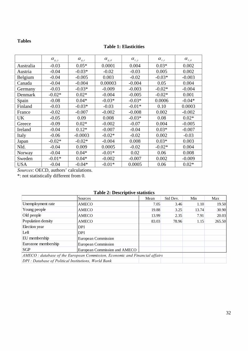
The values of elasticities are reported in Table 1. Expected signs are the following. Public
spending (on GDP) should decrease contemporaneously with GDP, and should increase
14
contemporaneously with long term interest rates (provided public debt is mostly financed
at floating rates), but the sign of the elasticity of public spending (on GDP) towards
inflation depends on the indexation of public spending on actual inflation. The sign of the
elasticity of tax receipts (on GDP) towards GDP depends on the tax structure: the more
progressive the tax system, the larger (and positive) the elasticity; if taxes are lump-sum
or exemptions are numerous, the elasticity can be negative: higher growth means lower
tax receipts in proportion of GDP. Tax receipts (on GDP) should respond positively,
provided net interests are charged with taxes; however, the sign of the related elasticity
could as well be indeterminate, as a higher long term interest rate also reduces the values
of bonds and stocks; consequently, reduced wealth can lead to lower tax receipts. Finally,
the elasticity of tax receipts (on GDP) towards inflation depends on the indexation
procedure of tax brackets.
Insert Table 1
Reported elasticities give a very diverse picture for the different countries involved under
review. It is noteworthy that the sole elasticity which sign is clearly determinate, ,g yα , is
always negative, as expected, and statistically significant for most countries. Other
elasticities testify for variations between countries in terms of degrees of indexation and
tax structures. The contemporaneous impact of long term interest rates on public
spending is often not statistically significant. This is not surprising as one can expect a
relative inertia of total public spending vis-à-vis a short term change in the nominal long
term interest rate.
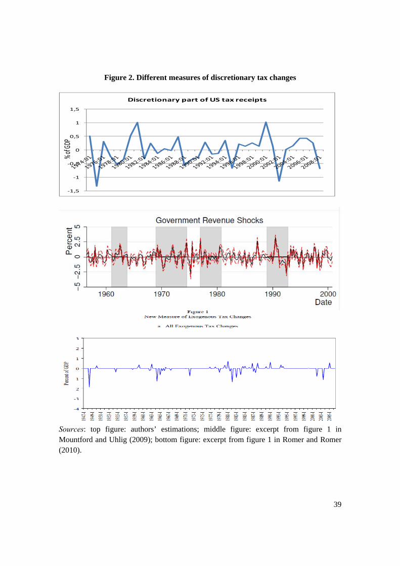
Estimated discretionary parts of public spending and tax receipts are presented in the
appendix for the 18 countries of the sample. As a matter of comparison, we report in
figure 2 the government revenue shocks estimated by Mountford and Uhlig (2009),
exogenous tax changes computed by Romer and Romer (2010), and our estimated
discretionary part of tax receipts, all three in the case of the US. At first sight, our method
gives frequent tax shocks, like Mountford and Uhlig (2009). A closer look shows that the
three methods point to a discretionary increase in taxes in 1981, 1987 and 1991, and to a
15
decrease in 1982 and 1988. All in all, our method gives consistent results with other
methods.
Insert Figure 2
Given the results obtained in this first step, we now turn to the investigation of the
potential spatial interactions between the sample countries.
2. Assessing fiscal policy interactions between OECD countries
Traditionally, empirical models of public policies relate public spending or tax receipts to
variables reflecting socio-economic and political characteristics of the country (or
region). This amounts to assuming that fiscal policies are only influenced by observed
national features. Under a linear specification, such a view leads one to estimate the
following model: ,
, , ,CA ik t i t i t i tu X β λ λ ε= + + + with ,k g τ= (3)
where ,,
CA ik tu are the per capita discretionary spending (or tax receipts) of the 1,i N=
countries, X is the set of exogenous national socio-economic characteristics, λi is a
country fixed effect, λt is a period fixed effect and ε , a vector of i.i.d error terms.
However, strategic interactions among governments have been one of the central issues
in theoretical public finance for the two last decades at least (see the survey by Wilson,
1999). As a consequence, spatial econometric techniques have recently been used to
estimate inter-governmental interaction models (see Brueckner, 2003; Revelli, 2005).
Building on the spatial econometric method developed by Anselin (1988), the model in
equation (3) is then augmented to include the spatially lagged dependent variable: , ,
, , ,,CA i CA jk t i t i t i tk tu Wu Xρ β λ λ ε= + + + + with i j≠ (4)

16
In this spatially lagged model, W is a weight matrix that assigns “neighbors” to each
country; the spatial lagged variable WY is a weighted average of all other countries’ fiscal
policy, ρ being the spatial autoregressive coefficient, which gives the sign and the
intensity of the impact of “neighboring” fiscal policies on one country’s public decision.
A negative ρ will imply that expenditure spillovers explain the spatial correlation
between countries decisions (Brueckner, 2003; Revelli, 2005). On the contrary, when ρ
is positive, a form of imitation (mimicking, i.e. fiscal competition or yardstick
competition) explains the observed interaction. For example, in the presence of tax base
mobility, the fiscal policy of a government may affect the budget constraints of other
governments, through capital migration (Wilson, 1999). This is the fiscal competition for
mobile resources assumption. In the yardstick competition theory, information on the
fiscal policy of the neighbor governments acts as a yardstick for the electorate in any
given country. As a result, any country’s citizens will compare the performance of their
own policymakers to the neighboring ones. This encourages mimicking behavior from
governments, as they do not want to be stigmatized (Salmon, 1987; Besley and Case,
1995).
Finally, a spatial auto-correlation pattern may simply reflect common shocks affecting
public policy or the omission of variables (such as country characteristics) that are
spatially dependent (Manski, 1993). In this case, we have a spatial autoregressive process
in the error term, or a spatial error model: ,
, , ,CA ik t i t i t i tu X β λ λ ε= + + + and , ,,i t i tW j t mε γ ε= + (5)
where γ is the spatial correlation coefficient, W a weight matrix and m a vector of i.i.d.
error terms.
Turning to estimation techniques, Anselin (1988) shows that, due to an endogeneity bias,
OLS estimators are inconsistent when estimating spatial lag and spatial error models.
However, instrumental variables (IV) or maximum likelihood (ML) estimation methods
lead to consistent estimators (Brueckner, 2003; Elhorst, 2003).
17
The weight matrix, denoted W, defines the structure of the interaction, the
“neighborhood” among countries. Since an a priori definition of interaction may
arbitrarily influence the estimations results, we will test the robustness of our fiscal policy
interaction model by using five different criteria, i.e. five different weight matrices.
First, to test whether our results are not an artifact of the statistical procedure in which the
neighborhood variable picks up the effect of any random set of countries, we build an
intentionally absurd weighting scheme.
Traditionally, to test fiscal competition, yardstick competition or spillover effects in
which neighborhood is a central feature, most empirical papers use weight matrices based
on geographical distance or simple contiguity. Following the relevant empirical literature,
we have chosen a common geographical definition of neighborhood based on the
Euclidean distance between countries (dij).7 This scheme is given by the weight matrix
WDIST and imposes a smooth distance decay with weights wij, given by 1/dij when i is
different from j (otherwise wij = 0).
A third set of matrix is based on economic criteria8. We consider the case where countries
follow an economic leader, the latter being defined by her GDP per capita. The matrix
WGDPL assigns higher weights to countries j with higher GDP per capita: wij = GDPj
/ jjGDP∑ if i is different from j, and 0 otherwise. We are thus able to assess size effects.
We clearly set the leader country. Matrix USLEADER gives a coefficient equal to 1 if
country j is the United States and 0 otherwise. Trade flows between countries may also be
a source of mimicking. As for WTRADE , country i is closer to country j than to country k if
the share of trade with j is higher than the share of trade with k in the total trade of
country i.
7 Geodesic distances are calculated following the great circle formula, which uses the geographic coordinates of the capital cities (CEPII data base). 8 See Case et al. (1993) and Baicker (2005) for a discussion on these matrices, defining similarities between countries in terms of income, population, etc.
18
It is conventional in the empirical spatial literature that all these weight matrices are
standardized so that the elements of each row sum to 1. Besides, we also include in our
model some control variables reflecting the impact of differences in socio-economic and
political factors grouped in the vector X in (3). Following the empirical literature, we
include some explanatory variables that might affect fiscal policies. We expect no
important impact of these variables, in validation of the first step of the empirical
procedure. It has to be noted that the economic resource variables such as GDP per
capita, which can be used as a measure of country income, have been removed from this
step in the empirical procedure since it was already included in the first one (see above).
Our data set includes the above 18 OECD countries, considered over a period of 34 years
(1975-2008). Descriptive statistics are shown in Table 2 in appendix.
The first data set of control variables, as is traditional in the literature, is composed of
socio-demographic variables, such as unemployment rate, population density, and shares
of under 14 (young people) and over 65 year-old in the population (old people). All these
variables are available from the AMECO database (European Commission, Economic
and Financial affairs). They are expected to exhibit a positive sign as they might reflect
higher needs of the population they designate. The variable (old people) is designed to
capture the political demand for social services by the older members of the electorate.
This segment of the population constitutes an interest group with growing political
power, and the variable (old people) is expected to be positively related to the size of the
government.
A second group of control variables includes political data collected from the Database of
Political Institutions (DPI, see Beck et al., 2001). Left is a dummy variable for the
country partisan affiliation, which takes the value 1 if the chief executive of country i in
year t belongs to a left-wing party, and 0 otherwise. We also introduce dummies for the
electoral cycle. Election year (t) is a dummy variable, which takes the value 1 if there is a
legislative election in year t. Election year t-1 (resp. t+1) is a dummy variable, which
19
takes the value 1 the year before (resp. after) the legislative election, and zero otherwise.
If there is a trend for an opportunistic political business cycle during the legislative
legislature, we will observe higher discretionary public spending and lower tax receipts
the year before the election or the election year.
As 13 countries of our sample are members of the European Union, the last group of
explanatory variables deals with EU features. We introduce three dummies respectively
for EU membership, for Eurozone membership and for the respect of the Stability and
Growth Pact (SGP). EU membership and Eurozone membership take the value 1 if the
country i in year t belongs respectively to the EU and to the Eurozone, zero otherwise.
SGP takes the value 1 if the EU country i’s deficit does not respect the SGP in year t, and
zero otherwise. A negative (positive) sign for this parameter will appear if the SGP is a
constraint or a disciplining device for the manipulation of discretionary spending (taxes)
in EU countries experimenting high deficits. Conversely, a positive (negative) sign will
emphasize the ineffectiveness of the disciplining device for discretionary spending
(taxes).
Our estimation strategy is as follows. We first estimate (3) using OLS without taking into
account the potential influence of the fiscal policy set by other countries. Because serial
correlation in panel data models biases the standard errors and causes the results to be
less efficient, we performed the Wooldridge test (2002) to identify potential serial
correlation in the idiosyncratic error term. This test does not detect the presence of such
correlation. We then run the appropriate spatial tests based on the Lagrange multiplier
tests in their robust version, which can detect the presence of spatial lag dependence and
spatial error dependence (see Anselin et al., 1996). We also use them in their robust
version which means that the robust LM-lag tests for lag dependency in presence of
missing error and the robust LM-ERR tests for error dependence in presence of missing
lag. If the LM test for spatial lag is more significant than the LM test for spatial error, and
the robust LM test for spatial lag is significant but the robust LM test for spatial error is
20
not, then the appropriate model is the spatial lag model (Anselin and Florax, 1995).9 We
find spatial lag dependency for all the weighting schemes we consider.10
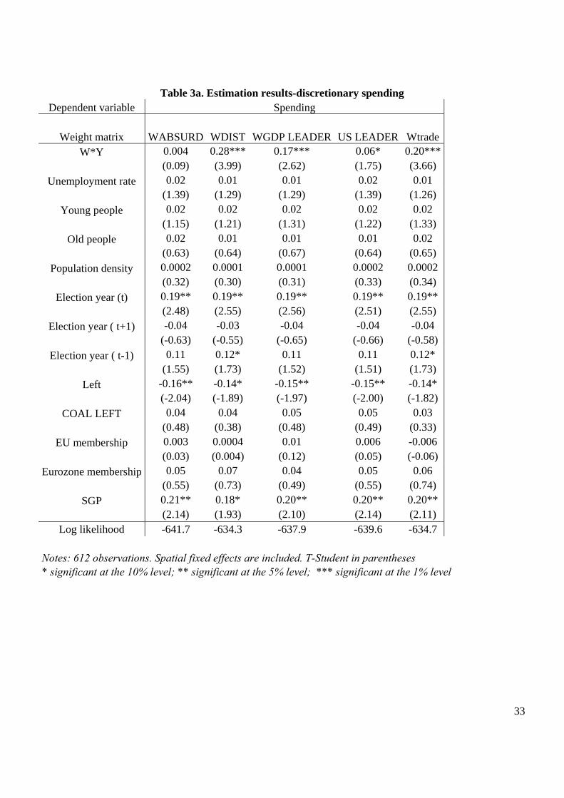
We then estimate the full model (4), the Y variable being our first step uCA residuals,
taking into account the influence of the other countries’ fiscal policies (weighted
spending decisions or tax receipts) using the maximum likelihood (ML) method.11 As
macroeconomic shocks that could be common to all countries have already been taken
into account in the first step of the empirical procedure, we do not need to include time
dummies. Estimation results for discretionary spending decisions and tax receipts are
shown in Tables 3a and 3b.
Insert Table 3a
Insert Table 3b
According to estimates reported in tables 4a and 4b, we find both a significant and
positive sign for the coefficient associated with the “neighboring” OECD countries'
decisions in discretionary public expenditures and tax receipts, except for the absurd
matrix. The estimation results confirm the existence of fiscal policy interactions for all
weighting schemes, either based on geographical proximity or on economic leadership.
This implies that geographically close countries tend to imitate each other, when they set
their discretionary fiscal policy. Countries also mimic their main trade partners and
9 Conversely, if the LM test for spatial error is more significant than the LM test for spatial lag and the robust LM test for spatial error is significant but the robust LM test for spatial lag is not, then the appropriate specification is the spatial error model. 10 LM tests estimation results are not shown in this paper, but are available upon request from the authors. 11 Furthermore, the normality of the residuals (the dependent variables) cannot be rejected, as the Shapiro-Wilk reveals (not shown here for space convenience but available on request). Non-normality could include overall skewness, overall tail weight differing from normal, individual outliers. Shapiro-Wilk test collapses all that onto one dimension by quantifying the straightness of a normal probability plot. The departure from a normal distribution is not statistically significant using this test.
21
economic leaders in the OECD like the US12. However, there is no interaction using the
absurd alphabetical matrix. This outcome confirms that our results are not an artifact of
the statistical procedure nor the effect of common shocks to countries of our sample but
come from mimicking between countries.
Result 1: There are some discretionary fiscal policy interactions between OECD
countries. Countries tend to imitate their geographical neighbours, their trade
partners and the economic leader of the area when they set their discretionary
public spending or tax receipts.
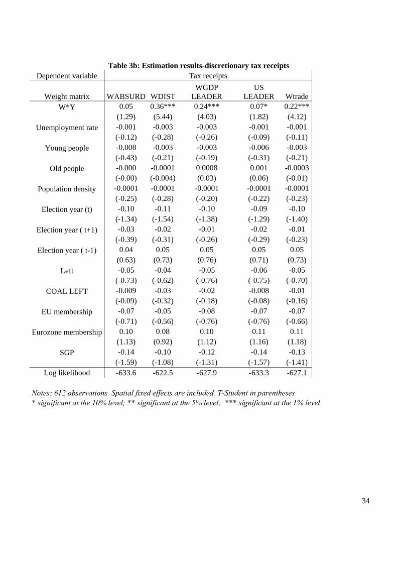
Let us now turn to the estimation results associated with the other explanatory variables.
Although no parameter associated with the socio-economic or political explanatory
variables is significant for tax receipts (a logical result, and a further proof of the fact that
our measure of discretionary fiscal policy really measures discretion), two important
results for public spending can be put to the fore.
First, dummies associated with legislative election years indicate an opportunistic use
(meaning, an increase) of discretionary public spending during the election year. This
gives strong evidence of a political budget cycle for discretionary public expenditures.
This result contradicts Brender and Drazen (2005, 2007), who find a political deficit
cycle in a large cross-section of 74 to 106 countries, a result which is driven by the
experience of “new democracies”. In contrast, our sample contains "mature"
democracries. Though we rehabilitate opportunistic cycles in older democracies, it has
thus to be recalled that our measure of fiscal policy draws on discretionary fiscal policy,
whereas Brender and Drazen (2005, 2007) use an overall deficit, i.e. the difference
between receipts and expenditures. Moreover, our measure does not allow to differentiate
between measures that may be more “visible” for voters than others, and thus measures
12 We also check if other countries are mimicked by all other countries. We find that interactions in discretionary tax receipts are significant at 5% with Germany, Ireland and Netherlands as leader. Results are available upon request.
22
that may be more or less effective, from the incumbent’s point of view (see Drazen and
Eslava, 2010).
Result 2: There is evidence of an opportunistic behavior of OECD countries'
governments for the discretionary public spending.
Second, we find evidence of ideological effects on the discretionary spending decisions,
as the coefficient of the partisan affiliation (Left) for the chief executive is significant and
negative. Left-wing chief executives seem to set lower discretionary public expenditures
than right-wing chief executives. As shown by the coefficient on the COAL*LEFT
variable, this result is not driven by the fact that Left-wing governments are more often
than their Right-wing counterpart, members of a ruling coalition.
Empirics on the relationship between partisan politics and public finance, drawing on a
panel of advanced economies, have generally come to mixed results (see Cusack, 1999,
for a survey). Stated briefly, some showed that left-wing governments were more
favorably inclined to high deficits or spending (see Cusack, 1997), though their influence
was a small one in comparison with right-wing governments (see Blais et al., 1993,
1996), whereas some argued that such an influence was contingent on macroeconomic
conditions (Carlsen, 1997; Cusack, 1999) and has decreased over time with the larger
openness of advanced economies (Cusack, 1999). In a recent paper dedicated to public
budgeting in France, Baumgartner et al. (2009) show that since 1981, no matter which
political type of government has been in power, limited growth in spending has been the
rule. Because right-wing governments had always been in power between 1958 and 1981,
Baumgartner et al. (2009) show that though differences are small, right-wing
governments have been the highest spenders.
Hence, our result is not completely surprising. Contrary to the above-mentioned
literature, it stems from the use of discretionary fiscal measures and thus does not hinge
23
on spending measures like unemployment benefits which are supposedly of greater
matter for left-wing governments than for right-wing ones, supposedly weighing the costs
of inflation higher. As a matter of fact, a complementary interpretation of the negative
coefficient associated with the (Left) variable, could be that left-wing governments are
more concerned than right-wing ones by the policy consequences of discretionary fiscal
policy. On the contrary, right-wing governments could be more prone to use such a
policy if they think it is associated with political (electoral) gains, along the lines of
Gilardi’s results (2010) with unemployment benefit policy. Moreover, our result is not
surprising if a strategic use of debt exists, à la Persson and Svensson (1989), a hypothesis
that can be consistent with this result and could not have been exhibited before. Overall
public spending might well be raised by incumbents, hence feeding debt growth, if they
fear they will not be reelected, hence newly elected governments have no choice but to
reduce spending whatever the economic conditions: discretionary public spending must
fall. Our result would fit this analysis provided the incumbent would come from the
Right, whereas the newly elected government would come from the Left.
Result 3: Left-wing chief executives set lower discretionary public spending.
The remaining explanatory variables based on socio-demographic features
(unemployment rate, young people, old people, and population densities) and on
European characteristics (EU and Eurozone memberships dummies) exhibit the expected
sign though they never appear as significant. Once again, this confirms that only the
discretionary components of fiscal policy are present in our dependent variables (i.e., the
first step has purged the fiscal data and our measure correctly estimates discretionary
impulses). The only significant explanatory variable is the SGP dummy, which sign is
positive in the discretionary public spending equation. The sign is consistently negative
in the discretionary tax revenues equation, though it is not statistically significant. The
coefficient on the SGP dummy shows that the EU fiscal framework is not effective in
prompting a corrective effect when public deficits in the EU are above the SGP threshold.
The disciplining device of the SGP is not working. This result complements Fatás and

24
Mihov (2003), who show that once countries are under the 3% threshold the incentives to
go further (towards the final objective of close to balance or surplus budgets) are much
weaker and countries reduce their efforts.
3. Further results
In this section, we first investigate the source of interdependence in national discretionary
fiscal policies (4.1) and second, we check whether the belonging to the EU matters (4.2).
3.1. How to interpret the existence of interactions between OECD fiscal policies?
We here investigate more deeply the source of interdependence in national discretionary
fiscal policies. As stressed by Redoano (2007), the coefficient associated with the
interaction term is not negative, so our results are not supportive of spillovers caused by
free riding behaviors. However, the positive interaction coefficient may come from fiscal
competition, yardstick competition, a common trend or may be the effect of similar
exogenous shocks.
First we can easily give up the last two explanations as the absurd matrix shows no sign
of interactions. Second, to distinguish between fiscal competition and yardstick
competition, we have to check if the spatial effect is stronger in election year. Yardstick
competition occurs when citizens compare fiscal and spending decisions made by their
incumbent with those of their neighbours (Salmon, 1987; Besley and Case, 1995). In this
context, policy-makers will be particularly concerned about neighbour incumbents in
election periods, and strategic interactions might be stronger at such times. A
straightforward way of testing this hypothesis is to use election cycle variables (Redoano,
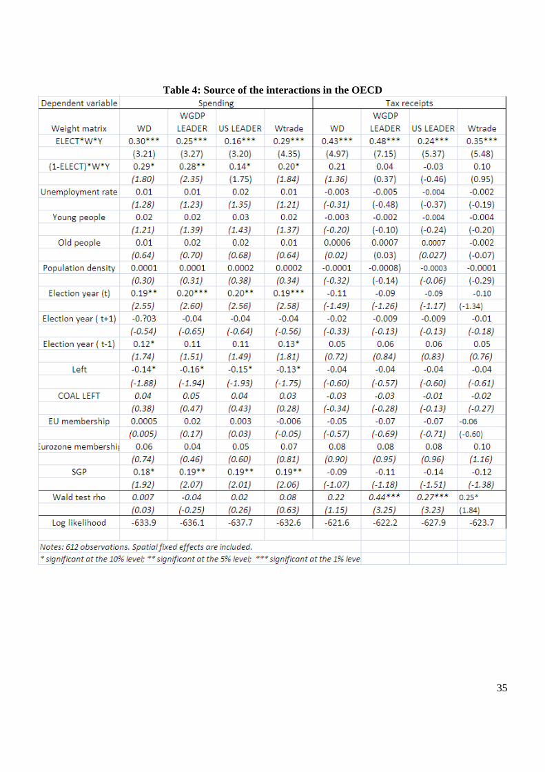
2007; Solé-Ollé, 2003). We interact the weighted average discretionary policy of
neighbours (Yj,t) with an election dummy (D) and estimate two interaction coefficients,
25
one for the year of election ( 1ρ ) and one for the rest of the period( 2ρ ). We thus need to
use a two-regime spatial lag model: , , ,
, 1 2 , ,, ,(1 )CA i CA j CA jk t i t i t i tk t k tu DWu D Wu Xρ ρ β λ λ ε= + − + + + + (6)
In line with Elhorst and Fréret (2009), we use a ML estimator to deal with this specific
model. Results are reported in Table 4 in appendix. We do not find a significant
difference in interactions in discretionary spending. However, highly significant
differences in the spatial interaction coefficient are found for the discretionary tax
receipts. OECD countries mimic discretionary revenues of the economic leaders of the
area (all GDP leaders or only US). The yardstick competition hypothesis cannot be
rejected for discretionary tax receipts.
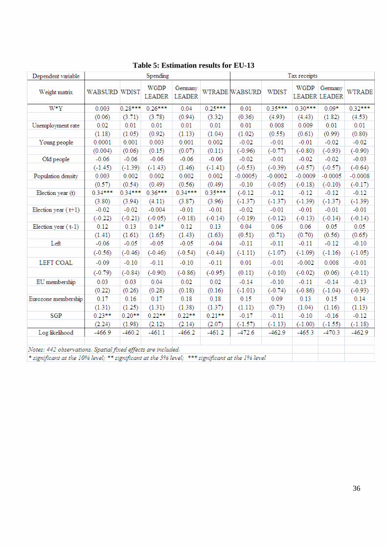
3.2. Does the EU matter?
Since 13 countries of our sample are EU members, we estimate equation (4) on a
subsample of European countries. The estimation results, shown in Table 5 in appendix,
confirm the robustness of the results found in tables 4a and 4b, while the political cycle
coefficients appear stronger for the European countries than for the whole sample. The
coefficient of the SGP dummy is also very robust to different specifications regarding the
weight matrices and the different samples.
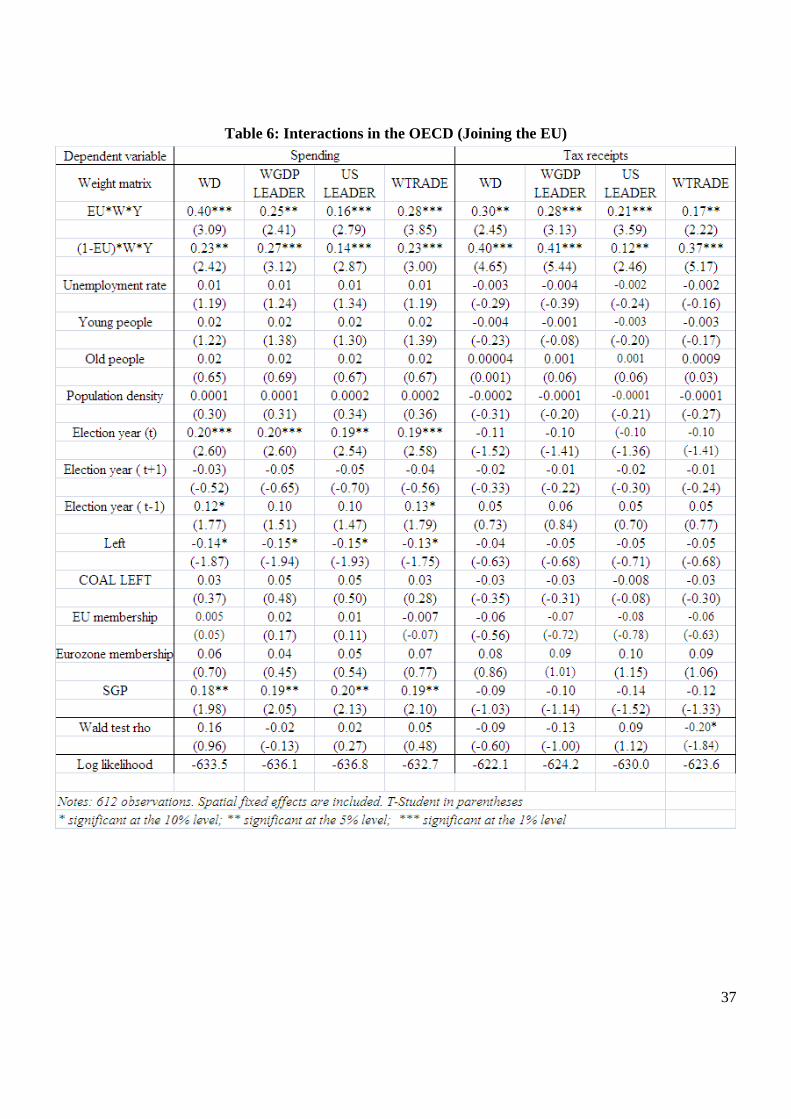
Another way to test if the EU matters in the interdependence of fiscal policy decisions is
to allow two interaction coefficients whether the country i belongs or not to the EU in the
full sample. We then estimate equation (6) on the full sample using as a dummy D for EU
membership. In our dataset, 8 countries were EU members while at the end of the period,
13 out of 18 are members of the EU. On the one hand, EU membership may cause more
interdependent decisions between countries, as countries are constrained in the policy
tools available to compete with other European countries. As stated by Redoano (2007):
“they move in a similar competitive and institutional environment and are subject to
26
similar budget and political constraints, moreover policy makers have more occasions to
meet and discuss formally or informally their plans”. On the other hand, EU non
members may engage in a more competitive behavior than EU countries, especially if
they want to convince EU states to accept their future membership. Table 6 (in appendix)
shows that the degree of interaction does not differ whether the country belongs or not to
the EU. This result is obtained for both measures of discretionary policy.
4. Conclusion
In this paper, we investigate the relationships between the discretionary components of
fiscal policies, for a sample of 18 OECD countries, during the 1974-2008 period. In a
first step, we build two indicators of discretionary fiscal policy, considered as the residual
components of a VAR model: one for public spending, and one for tax receipts.
The second step provides estimates of discretionary fiscal policy interactions between
these OECD countries using spatial econometrics. Our results confirm the existence of
interactions between neighboring countries’ public decisions, where neighborhood is
defined by economic proximity as well as by geography. We also find evidence of an
opportunistic behavior of OECD countries’ governments for the discretionary public
spending, even stronger for the sub-sample of European countries. Moreover, left-wing
chief executives seem to set lower discretionary public expenditures than right-wing chief
executives, which could reveal the presence of a strategic use of deficits by right-wing
incumbents. Finally, the disciplining device of the European Union fiscal framework is
shown to be ineffective. Future research may be to investigate the link between public
spending and tax receipts.
27
Acknowledgements
The authors acknowledge financial assistance from the French National Research Agency (grant FRAL022). They have benefited from comments by Cristina Badarau-Semenescu, Lars Borge, Martial Foucault, Jean-Luc Gaffard, Marcel Gérard, Jurgen von Hagen, Hakim Hammadou, Jérôme Héricourt, Grégory Levieuge, Ioana Moldovan, Edoardo di Porto, Laurence Rioux, Blandine Zimmer, participants in the Public Economics Day (Paris 1), the European Public Choice Society 2010 meeting, the 44th Canadian Economics Association conference, Journées AFSE 2010, the 27th symposium on Money Banking and Finance Bordeaux 2010, AFSE Annual Conference 2010, and seminar participants in Bonn. The usual disclaimer applies.
References
Agnello, L., Cimadomo, J., 2009. Discretionary Fiscal Policies over the Cycle: New Evidence based on the ESCB Disaggregated Approach. Working Paper 1118, European Central Bank.
Anselin, L., 1988. Spatial econometrics: Methods and models. Dordrecht: Kluwer Academic.
Anselin, L., Bera, A.K., Florax, R., Yoon., M. J., 1996. Simple diagnostic tests for spatial dependence. Regional Science and Urban Economics 26,77-104.
Anselin, L., Florax, R., 1995. New Directions in Spatial Econometrics, Springer, Berlin et al. loc.
Baicker, K., 2005. The Spillover Effects of State Spending. Journal of Public Economics 89, 529–544.
Baumgartner, F.R., Foucault, M., François, A., 2009. Public budgeting in the French Fifth Republic: the end of “La République des partis” ? West European Politics 32(2), 404-422.
Beck, T., Clarke, G., Groff, A., Keefer, P., Walsh, P., 2001. New tools in comparative political economy: The Database of Political Institutions. World Bank Economic Review 15:1, 165-176.
Beetsma, R., Giuliodori, M., 2010a. Fiscal adjustment to cyclical developments in the OECD: an empirical analysis based on real-time data. Oxford Economic Papers, 419-441.
Beetsma, R., Giuliodori, M., 2010b. Discretionary fiscal policy: review and estimates for the EU. CesIfo Working Paper 2948.
Benetrix, A.S., Lane P., The impact of fiscal shocks on the Irish economy. The Economic and Social Review 40(4), 407-434.
Besley, T., Case, A., 1995. Incumbent Behavior: Vote Seeking, Tax Setting and Yardstick Competition. American Economic Review 85, 25–45.
Biau, O., Girard, E., 2005. Politique budgétaire et dynamique économique en France: l’approche VAR Structurel. Revue économique 56(3), 755-64.

28
Blais, A., Blake, D., Dion, S., 1993. Do parties make a difference? Parties and the size of government in liberal democracies. American Journal of Political Science 37(1), 40-62.
Blais, A., Blake, D., Dion, S., 1996. Do parties make a difference? A reappraisal. American Journal of Political Science 40(2), 514-520.
Blanchard, O.J., Perotti, R., 2002. An Empirical Characterization of the Dynamic Effects of Changes in Government Spending and Taxes on Output. Quarterly Journal of Economics 117(4), 1329-68.
Brender, A., Drazen, A., 2005. Political budget cycles in new versus established democracies. Journal of Monetary Economics 52, 1271-1295
Brender, A., Drazen, A., 2007. Electoral Fiscal Policy in New, Old, and Fragile Democracies. Comparative Economic Studies 49, 446-466.
Brueckner, J., 2003. Strategic Interaction Among Governments: An Overview of Empirical Studies. International Regional Science Review 26, 175–188.
Burriel, P., de Castro, F., Garrote, D., Gordo, E., Paredes, J.,Perez, J.J., 2010. Fiscal policy shocks in the Euro area and the US: an empirical assessment. Fiscal Studies, forthcoming.
Canova, F., Pappa, E., 2007. Price differentials in monetary unions: the role of fiscal shocks. Economic Journal 117, 713-737.
Carlsen, F., 1997. Counterfiscal policies and partisan politics: evidence from industrialized countries. Applied Economics 29, 145-151.
Case, A., Hines, J., Rosen, H., 1993. Budget Spillovers and Fiscal Policy Interdependence. Journal of Public Economics 52, 285–307.
Creel, J., Monperrus-Veroni, P., Saraceno, F., 2009. Has the Golden Rule of public finance made a difference in the United Kingdom? Scottish Journal of Political Economy 56(5), 580-607.
Cusack, T.R., 1997. Partisan politics and public finance: changes in public spending in the industrialized democracies, 1955-1989. Public Choice 91, 375-395.
Cusack, T.R., 1999. Partisan politics and fiscal policy. Comparative Political Studies 32(4), 464-486.
Drazen, A., Eslava, M., 2010. Electoral manipulation via voter-friendly spending: Theory and evidence. Journal of Development Economics 92(1), 39-52.
Elhorst, J.P., 2003. Specification and Estimation of Spatial Panel Data Models. International Regional Science Review 26, 244-268.
Elhorst, J.P., Fréret, S., 2009. Evidence of political yardstick competition in France using a two- regime spatial Durbin model with fixed effects. Journal of Regional Science 49(5), pages 931-951.
Fatás, A., Mihov, I., 2003. On Constraining Fiscal Policy Discretion in EMU. Oxford Review of Economic Policy 19:1, 112-131.
29
Figlio, D. N., Kolpin, V. W., Reid, W. E., (1999). Do States play welfare games? Journal of Urban Economics 46, 437–454.
Gilardi, F., 2010. Who learns from what in policy diffusion processes. American Journal of Political Science 54:3, 650-666 Giordano, R., Momigliano, S., Neri, S, Perotti, R., 2007. The effects on the economy of shocks to different government expenditures items: estimates with a SVAR model. European Journal of Political Economy 23(3), 707-733.
Giuliodori, M., Beetsma, R., 2008. On the relationship between fiscal plans in the European Union: an empirical analysis based on real-time data. Journal of Comparative Economics 36, 221-242
Hallerberg, M., Strauch, R., von Hagen, J., 2009. Fiscal governance in Europe, Cambridge University Press
Lindbeck, A., 2008. Welfare State. New Palgrave Dictionary, 2nd edition, vol. 8, 731-738
Manski, C., 1993. Identification of Endogenous Social Effects: The Reflection Problem. Review of Economic Studies 60, 531–542.
Mountford, A., Uhlig, H., 2009. What are the effects of fiscal policy shocks? Journal of Applied Econometrics 24(6), 960-992.
Musgrave, R., 1966. Principles of Budget Determination. in H. Cameron and W. Henderson (eds.), Public Finance: Selected Readings, Random House.
Neely, Ch. J., Rapach, D. E., 2009. Common fluctuations in OECD budget balances. Working Papers 2009-055, Federal Reserve Bank of St. Louis
OECD, 2004. The legal framework for budget systems: an international comparison. OECD Journal on Budgeting, special issue 4(3).
Perotti, R., 2004. Public investment: Another (Different) Look. IGIER Working Paper 277, Bocconi University, December.
Persson, T., Svensson, L., 1989. Why a stubborn conservative would run a deficit: policy with time-inconsistent preferences. Quarterly Journal of Economics 104.
Ramey, V.A., Shapiro, M.D., 1998. Costly capital reallocation and the effects of government spending. Carnegie-Rochester Conference Series on Public Policy 48(1), 145-194.
Redoano, M., 2003. Fiscal interactions among European countries. Warwick Economic research papers 680.
Redoano, M. (2007). Fiscal interactions among European countries. Does the EU matter? CESIFO Working paper No. 1952, March.
Romer, C., Romer, D., 1989. Does Monetary Policy Matter? A New Test in the Spirit of Friedman and Schwartz. NBER Macroeconomics Annual, 4, 121-170
Romer, C., Romer, D., 2009. Do tax cuts starve the beast? The effect of tax changes on government spending. Brookings Papers on Economic Activity 1, 139-200
30
Romer, C., Romer, D., 2010. The macroeconomic effects of tax changes: estimates based on a new measure of fiscal shocks. American Economic Review 100, 763-801.
Revelli, F., 2005. On spatial public finance empirics. International Tax and Public Finance 12, 475-492.
Oudiz, G., Sachs, J.D., 1984. Macroeconomic policy coordination among the industrial economies. Brookings Papers on Economic Activity 1, 1-75.
Salmon, P., 1987. Decentralization as an incentive scheme. Oxford Review of Economic Policy 3, 24-43.
Steiner, A., 2010. Contagious policies: an analysis of spatial interactions among countries' capital account policies. Pacific Economic Review 15(3), 422-445.
Wilson, J., 1999. Theories of Tax Competition. National Tax Journal 53, 269–304.
Wooldridge, J.M., 2002. Econometric Analysis of Cross Section and Panel Data. Cambridge, MA: MIT Press.
31
Appendix Insert Table 2 Insert Table 4 Insert Table 5 Insert Table 6
32
Tables Table 1: Elasticities
,g yα ,g rα ,g πα , yτα ,rτα ,τ πα Australia -0.03 0.05* 0.0001 0.004 0.03* 0.002 Austria -0.04 -0.03* -0.02 -0.03 0.005 0.002 Belgium -0.04 -0.005 0.003 -0.02 -0.03* -0.003 Canada -0.04 -0.004 0.00003 -0.004 0.05 0.004 Germany -0.03 -0.03* -0.009 -0.003 -0.02* -0.004 Denmark -0.02* 0.02* -0.004 -0.005 -0.02* 0.001 Spain -0.08 0.04* -0.03* -0.03* 0.0006 -0.04* Finland -0.03 -0.03* -0.03 -0.01* 0.10 0.0003 France -0.02 -0.007 -0.002 -0.008 0.002 -0.002 UK -0.05 0.09 0.008 -0.03* 0.08 0.02* Greece -0.09 0.02* -0.002 -0.07 0.004 -0.005 Ireland -0.04 0.12* -0.007 -0.04 0.03* -0.007 Italy -0.06 -0.0003 -0.02* -0.02 0.002 -0.03 Japan -0.02* -0.02* -0.004 0.008 0.03* 0.003 Nld. -0.04 0.009 0.0005 -0.02 -0.02* 0.004 Norway -0.04 0.04* -0.01* 0.02 0.06 0.008 Sweden -0.01* 0.04* -0.002 -0.007 0.002 -0.009 USA -0.04 -0.04* -0.01* 0.0005 0.06 0.02* Sources: OECD, authors’ calculations. *: not statistically different from 0.
Table 2: Descriptive statistics
Sources Mean Std Dev. Min MaxUnemployment rate AMECO 7.05 3.46 1.10 19.50Young people AMECO 19.88 3.25 13.74 30.90Old people AMECO 13.99 2.35 7.91 20.03Population density AMECO 83.03 78.96 1.15 265.50Election year DPILeft DPIEU membership European CommissionEurozone membership European CommissionSGP European Commission and AMECOAMECO : database of the European Commission, Economic and Financial affairsDPI : Database of Political Institutions, World Bank
33
Table 3a. Estimation results-discretionary spending Dependent variable Spending
Weight matrix WABSURD WDIST WGDP LEADER US LEADER Wtrade W*Y 0.004 0.28*** 0.17*** 0.06* 0.20***
(0.09) (3.99) (2.62) (1.75) (3.66) Unemployment rate 0.02 0.01 0.01 0.02 0.01
(1.39) (1.29) (1.29) (1.39) (1.26) Young people 0.02 0.02 0.02 0.02 0.02
(1.15) (1.21) (1.31) (1.22) (1.33) Old people 0.02 0.01 0.01 0.01 0.02
(0.63) (0.64) (0.67) (0.64) (0.65) Population density 0.0002 0.0001 0.0001 0.0002 0.0002
(0.32) (0.30) (0.31) (0.33) (0.34) Election year (t) 0.19** 0.19** 0.19** 0.19** 0.19**
(2.48) (2.55) (2.56) (2.51) (2.55) Election year ( t+1) -0.04 -0.03 -0.04 -0.04 -0.04
(-0.63) (-0.55) (-0.65) (-0.66) (-0.58) Election year ( t-1) 0.11 0.12* 0.11 0.11 0.12*
(1.55) (1.73) (1.52) (1.51) (1.73) Left -0.16** -0.14* -0.15** -0.15** -0.14*
(-2.04) (-1.89) (-1.97) (-2.00) (-1.82) COAL LEFT 0.04 0.04 0.05 0.05 0.03
(0.48) (0.38) (0.48) (0.49) (0.33) EU membership 0.003 0.0004 0.01 0.006 -0.006
(0.03) (0.004) (0.12) (0.05) (-0.06) Eurozone membership 0.05 0.07 0.04 0.05 0.06
(0.55) (0.73) (0.49) (0.55) (0.74) SGP 0.21** 0.18* 0.20** 0.20** 0.20**
(2.14) (1.93) (2.10) (2.14) (2.11) Log likelihood -641.7 -634.3 -637.9 -639.6 -634.7
Notes: 612 observations. Spatial fixed effects are included. T-Student in parentheses * significant at the 10% level; ** significant at the 5% level; *** significant at the 1% level
34
Table 3b: Estimation results-discretionary tax receipts Dependent variable Tax receipts
Weight matrix WABSURD WDISTWGDP
LEADER US
LEADER Wtrade W*Y 0.05 0.36*** 0.24*** 0.07* 0.22***
(1.29) (5.44) (4.03) (1.82) (4.12) Unemployment rate -0.001 -0.003 -0.003 -0.001 -0.001
(-0.12) (-0.28) (-0.26) (-0.09) (-0.11) Young people -0.008 -0.003 -0.003 -0.006 -0.003
(-0.43) (-0.21) (-0.19) (-0.31) (-0.21) Old people -0.000 -0.0001 0.0008 0.001 -0.0003
(-0.00) (-0.004) (0.03) (0.06) (-0.01) Population density -0.0001 -0.0001 -0.0001 -0.0001 -0.0001
(-0.25) (-0.28) (-0.20) (-0.22) (-0.23) Election year (t) -0.10 -0.11 -0.10 -0.09 -0.10
(-1.34) (-1.54) (-1.38) (-1.29) (-1.40) Election year ( t+1) -0.03 -0.02 -0.01 -0.02 -0.01
(-0.39) (-0.31) (-0.26) (-0.29) (-0.23) Election year ( t-1) 0.04 0.05 0.05 0.05 0.05
(0.63) (0.73) (0.76) (0.71) (0.73) Left -0.05 -0.04 -0.05 -0.06 -0.05
(-0.73) (-0.62) (-0.76) (-0.75) (-0.70) COAL LEFT -0.009 -0.03 -0.02 -0.008 -0.01
(-0.09) (-0.32) (-0.18) (-0.08) (-0.16) EU membership -0.07 -0.05 -0.08 -0.07 -0.07
(-0.71) (-0.56) (-0.76) (-0.76) (-0.66) Eurozone membership 0.10 0.08 0.10 0.11 0.11
(1.13) (0.92) (1.12) (1.16) (1.18) SGP -0.14 -0.10 -0.12 -0.14 -0.13
(-1.59) (-1.08) (-1.31) (-1.57) (-1.41) Log likelihood -633.6 -622.5 -627.9 -633.3 -627.1
Notes: 612 observations. Spatial fixed effects are included. T-Student in parentheses * significant at the 10% level; ** significant at the 5% level; *** significant at the 1% level
35
Table 4: Source of the interactions in the OECD
36
Table 5: Estimation results for EU-13
37
Table 6: Interactions in the OECD (Joining the EU)

38
Figures
Figure 1.
-50
-40
-30
-20
-10
0
10
20
-8
-6
-4
-2
0
2
4
6
8
2007q1 2007q2 2007q3 2007q4 2008q1 2008q2 2008q3 2008q4 2009q1 2009q2 2009q3 2009q4
US Business cycle, 2007-2009
GDP
Consumption
Nonresidential Inv. (right axis)
Source: US Bureau of Economic Analysis.
39
Figure 2. Different measures of discretionary tax changes
‐1,5
‐1
‐0,5
0
0,5
1
1,5
Discretionary part of US tax receipts
% ofG
DP
Sources: top figure: authors’ estimations; middle figure: excerpt from figure 1 in Mountford and Uhlig (2009); bottom figure: excerpt from figure 1 in Romer and Romer (2010).