1
Chapter 4Instructor: Hossein Pourghassem
Image Enhancement in theFrequency Domain
2
Fourier Series

2
Islamic Azad University of Najafabad, Department of Electrical Engineering, Dr. H. Pourghassem, 3
Fourier Series
Fourier series: a periodic function can be represented by the sum of sines/cosines of different frequencies, multiplied by a different coefficient (Fourier series)
Tu
uwnwtBnwtAxf
xfTxf
nn
12
)sin()cos()()()(
=
=
+=
=+
∑π
Islamic Azad University of Najafabad, Department of Electrical Engineering, Dr. H. Pourghassem, 4
One dimensional Fourier TransformNon-periodic functions can also be represented as the
integral of sines/cosines multiplied by weighting function (Fourier transform)f(x): continuous function of a real variable x
Fourier transform of f(x):
{ } ∫∞
∞−
−==ℑ dxuxjxfuFxf ]2exp[)()()( π
where 1−=j

3
Islamic Azad University of Najafabad, Department of Electrical Engineering, Dr. H. Pourghassem, 5
One dimensional Fourier Transform
Given F(u), f(x) can be obtained by the inverse Fourier transform:
)()}({1 xfuF =ℑ−
∫∞
∞−
= duuxjuF ]2exp[)( π
• The above two equations are the Fourier transform pair.
Islamic Azad University of Najafabad, Department of Electrical Engineering, Dr. H. Pourghassem, 6
Discrete Fourier Transform
A continuous function f(x) is discretized into a sequence:
)}]1[(),...,2(),(),({ 0000 xNxfxxfxxfxf Δ−+Δ+Δ+
by taking N or M samples Δx units apart.

4
Islamic Azad University of Najafabad, Department of Electrical Engineering, Dr. H. Pourghassem, 7
Discrete Fourier Transform
Where x assumes the discrete values (0,1,2,3,…,M-1) then
)()( 0 xxxfxf Δ+=
• The sequence {f(0),f(1),f(2),…f(M-1)} denotes any M uniformly spaced samples from a corresponding continuous function.
Islamic Azad University of Najafabad, Department of Electrical Engineering, Dr. H. Pourghassem, 8
Discrete Fourier Transform
∫
∑
−
−
+∞
−∞=
−
=
=
π
ππdweeFxf
exfeF
jwxjw
x
jwxjw
)(21)(
)()(
Fourier Transform of discrete function is a continuous functionwhich is calculated as follows:
5
Islamic Azad University of Najafabad, Department of Electrical Engineering, Dr. H. Pourghassem, 9
Discrete Fourier Transform
xwu
nFx
eFn
sjw
ΩΔ==Ω
Ω−ΩΔ
= ∑+∞
−∞=
π2
)(1)(
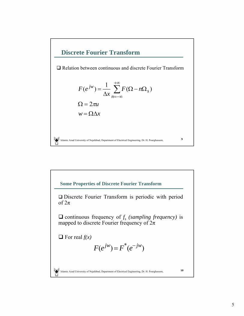
Relation between continuous and discrete Fourier Transform
Islamic Azad University of Najafabad, Department of Electrical Engineering, Dr. H. Pourghassem, 10
Some Properties of Discrete Fourier Transform
Discrete Fourier Transform is periodic with period of 2π
continuous frequency of fs (sampling frequency) is mapped to discrete Fourier frequency of 2π
For real f(x)
)()( * jwjw eFeF −=

6
Islamic Azad University of Najafabad, Department of Electrical Engineering, Dr. H. Pourghassem, 11
Discrete Fourier Transform
The values u = 0, 1, 2, …, M-1 correspond to samples of the continuous transform at values 0, Δu, 2Δu, …, (M-1)Δu.
i.e. F(u) represents F(uΔu), where:
Δu =1
MΔx
Islamic Azad University of Najafabad, Department of Electrical Engineering, Dr. H. Pourghassem, 12
Introduction to the Fourier Transform
The Fourier transform of a real function is generally complex and we use polar coordinates:
|F(u)| (magnitude function) is the Fourier spectrum of f(x) and φ(u) its phase angle.The square of the spectrum
is referred to as the power spectrum of f(x) (spectral density).
⎥⎦
⎤⎢⎣
⎡=
+=
=
+=
−
)()(tan)(
)]()([)(
)()()()()(
1
2/122
)(
uRuIu
uIuRuF
euFuFujIuRuF
uj
φ
φ
)()()()( 222 uIuRuFuP +==

7
Islamic Azad University of Najafabad, Department of Electrical Engineering, Dr. H. Pourghassem, 13
Two Dimensional Discrete Fourier Transform
In a 2-variable case, the discrete FT pair is:
∑∑−
=
−
=
+−=1
0
1
0
)]//(2exp[),(1),(M
x
N
y
NvyMuxjyxfMN
vuF π
∑∑−
=
−
=
+=1
0
1
0)]//(2exp[),(),(
M
u
N
vNvyMuxjvuFyxf π
For u=0,1,2,…,M-1 and v=0,1,2,…,N-1
For x=0,1,2,…,M-1 and y=0,1,2,…,N-1
AND:
Islamic Azad University of Najafabad, Department of Electrical Engineering, Dr. H. Pourghassem, 14
Discrete Fourier Transform
Sampling of a continuous function is now in a 2-D grid (Δx, Δy divisions).
The discrete function f(x,y) represents samples of the function f(x0+xΔx,y0+yΔy) for x=0,1,2,…,M-1 and y=0,1,2,…,N-1.
yNv
xMu
Δ=Δ
Δ=Δ
1 ,1

8
Islamic Azad University of Najafabad, Department of Electrical Engineering, Dr. H. Pourghassem, 15
Introduction to the Fourier Transform
Fourier spectrum: [ ] 2/122 ),(),(),( vuIvuRvuF +=
• Phase: ⎥⎦
⎤⎢⎣
⎡= −
),(),(tan),( 1
vuRvuIvuφ
• Power spectrum: ),(),(),(),( 222 vuIvuRvuFvuP +==
Islamic Azad University of Najafabad, Department of Electrical Engineering, Dr. H. Pourghassem, 16
Discrete Fourier Transform
When images are sampled in a square array, M=N and the FT pair becomes:
∑∑−
=
−
=
+−=1
0
1
0
]/)(2exp[),(1),(N
x
N
y
NvyuxjyxfN
vuF π
∑∑−
=
−
=
+=1
0
1
0]/)(2exp[),(1),(
N
u
N
vNvyuxjvuF
Nyxf π
For u,v=0,1,2,…,N-1
For x,y=0,1,2,…,N-1
AND:

9
Islamic Azad University of Najafabad, Department of Electrical Engineering, Dr. H. Pourghassem, 17
Basic Properties
F(0,0) is at u=M/2 and v=N/2Shifts the origin of F(u,v) to (M/2, N/2), i.e. the center of MxN of the 2-D DFT (frequency rectangle)Frequency rectangle: from u=0 to u=M-1, and v=0 to v=N-1 (u,v integers, M,N even numbers) In computers: summations are from u=1 to M and v=1 to N center of transform: u=(M/2) +1 and v=(N/2) +1
[ ] )2/,2/()1)(,( NvMuFyxf yx −−=−ℑ +
Common practice:
Islamic Azad University of Najafabad, Department of Electrical Engineering, Dr. H. Pourghassem, 18
Basic Properties
Value of transform at (u,v)=(0,0):
which means that the value of FT at the origin = the average gray level of the imageFT is also conjugate symmetric:
F(u,v)=F*(-u,-v)so |F(u,v)|=|F(-u,-v)|
which means that the FT spectrum is symmetric.
F(0,0) =1
MNf (x, y)
y= 0
N −1
∑x= 0
M −1
∑

10
Islamic Azad University of Najafabad, Department of Electrical Engineering, Dr. H. Pourghassem, 19
Basic Properties
Islamic Azad University of Najafabad, Department of Electrical Engineering, Dr. H. Pourghassem, 20
Image Enhancement in the Frequency Domain

11
Islamic Azad University of Najafabad, Department of Electrical Engineering, Dr. H. Pourghassem, 21
Basic steps for filtering in the frequency domain
1. Multiply input Image by (-1)x+y to center the transform,
2. Compute F(u,v) , the DFT of image
3. Multiply by a filter function H(u,v)
4. Compute inverse DFT of the result in (3)
5. Obtain the real part of result in (4)
6. Multiply the result in 5 by (-1)x+y
Summary: G(u,v) = H(u,v) F(u,v)
Filtered Image = ℑ−1 G(u,v)[ ]
Islamic Azad University of Najafabad, Department of Electrical Engineering, Dr. H. Pourghassem, 22
Basic steps for filtering in the frequency domain

12
Islamic Azad University of Najafabad, Department of Electrical Engineering, Dr. H. Pourghassem, 23
Edges and sharp transitions (e.g., noise) in an image contributesignificantly to high-frequency content of FT.
Low frequency contents in the FT are responsible to the general appearance of the image over smooth areas.
Blurring (smoothing) is achieved by attenuating range of high frequency components of FT.
Frequency Domain Filtering
Islamic Azad University of Najafabad, Department of Electrical Engineering, Dr. H. Pourghassem, 24
f(x,y) is the input imageg(x,y) is the filteredh(x,y): impulse response
Convolution Theorem
G(u,v)=F(u,v)●H(u,v)
g(x,y)=h(x,y)*f(x,y)
• Filtering in Frequency Domain with H(u,v) is equivalent to filtering in Spatial Domain with h(x,y).
Multiplication in Frequency Domain
Convolution in Time Domain
13
Islamic Azad University of Najafabad, Department of Electrical Engineering, Dr. H. Pourghassem, 25
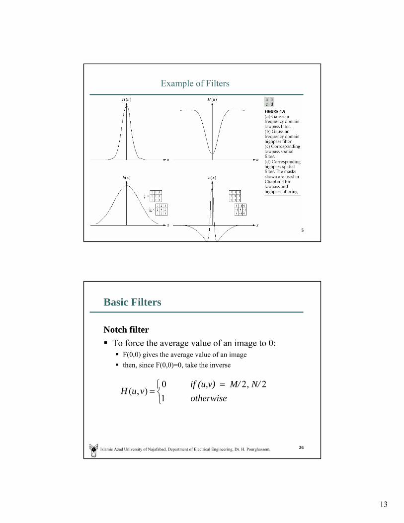
Example of Filters
Islamic Azad University of Najafabad, Department of Electrical Engineering, Dr. H. Pourghassem, 26
Basic Filters
Notch filterTo force the average value of an image to 0:
F(0,0) gives the average value of an imagethen, since F(0,0)=0, take the inverse
⎩⎨⎧ =
=otherwise
, N/ M/if (u,v) vuH
1220
),(

14
Islamic Azad University of Najafabad, Department of Electrical Engineering, Dr. H. Pourghassem, 27
Image Enhancement in the Frequency Domain
Islamic Azad University of Najafabad, Department of Electrical Engineering, Dr. H. Pourghassem, 28
Image Enhancement in the Frequency Domain
Types of enhancement that can be done:
Lowpass filtering: reduce the high-frequency content--blurring or smoothing
Highpass filtering: increase the magnitude of high-frequency components relative to low-frequency components -- sharpening.

15
Islamic Azad University of Najafabad, Department of Electrical Engineering, Dr. H. Pourghassem, 29
Image Enhancement in the Frequency Domain
Islamic Azad University of Najafabad, Department of Electrical Engineering, Dr. H. Pourghassem, 30
Low Pass filtering or Smoothing in the Frequency Domain
G(u,v) = H(u,v) F(u,v)IdealButterworth (parameter: filter order); for high and low values of this parameter, the Butterworth approaches the form of the ideal filter and Gaussian filter, respectively. Gaussian

16
Islamic Azad University of Najafabad, Department of Electrical Engineering, Dr. H. Pourghassem, 31
Ideal low-pass filter (ILPF)
D0 is called the cutoff frequency.
(M/2,N/2): center in frequency domain
2 2 1/2( , ) [( / 2) ( / 2) ]D u v u M v N= − + −⎩⎨⎧
>≤
=0
0
),(0),(1
),(DvuDDvuD
vuH
Islamic Azad University of Najafabad, Department of Electrical Engineering, Dr. H. Pourghassem, 32
Shape of ILPF
Spatial domain
Frequency domain

17
Islamic Azad University of Najafabad, Department of Electrical Engineering, Dr. H. Pourghassem, 33
Traditional Methodfor Calculation of Cutoff frequency
The summation is taken within the circle D0
⎥⎥⎦
⎤
⎢⎢⎣
⎡= ∑∑
u vTPvuP /),(100α
Calculate PT , the total Power of image
∑ ∑−
=
−
==
1
0
1
0),(
M
u
N
vT vuPP
A circle with radius D0, origin at the center of the frequency rectangle encloses a percentage of the power which is given by the expression
Islamic Azad University of Najafabad, Department of Electrical Engineering, Dr. H. Pourghassem, 34
Image Enhancement in the Frequency Domain

18
35
ringing and
blurring
36
Ringing
19
Islamic Azad University of Najafabad, Department of Electrical Engineering, Dr. H. Pourghassem, 37
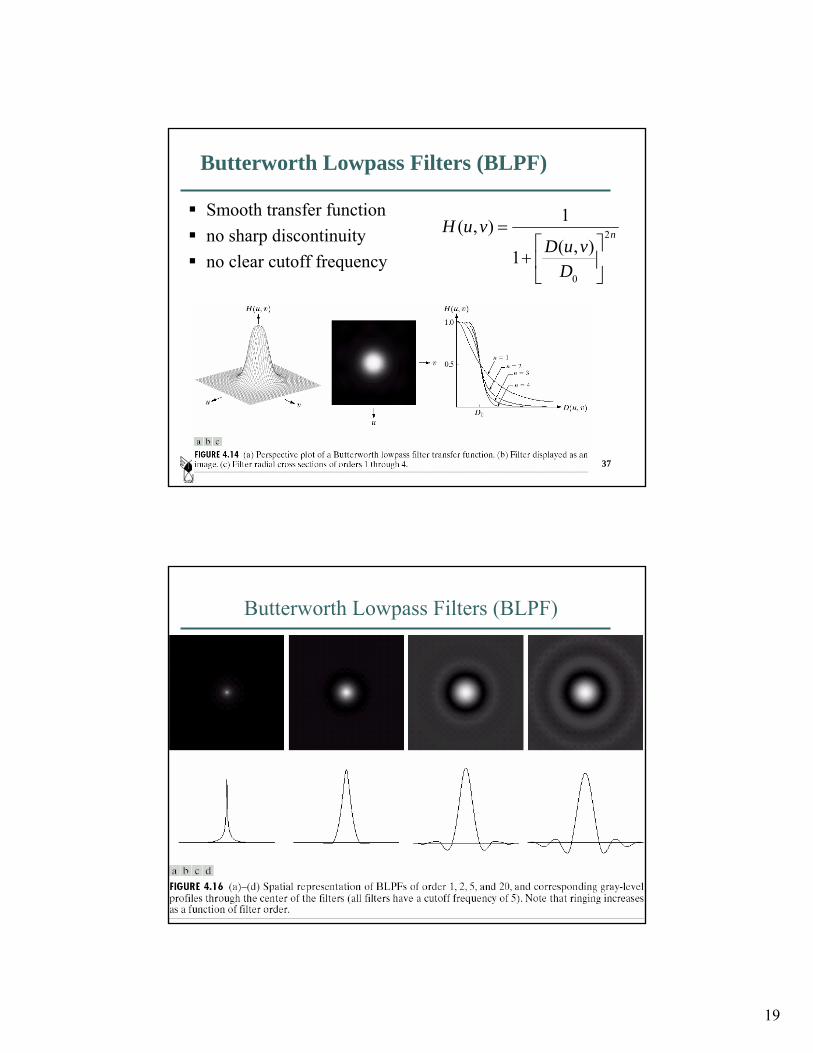
Butterworth Lowpass Filters (BLPF)
Smooth transfer functionno sharp discontinuity no clear cutoff frequency
n
DvuD
vuH 2
0
),(1
1),(
⎥⎦
⎤⎢⎣
⎡+
=
21
Islamic Azad University of Najafabad, Department of Electrical Engineering, Dr. H. Pourghassem, 38
Butterworth Lowpass Filters (BLPF)
20
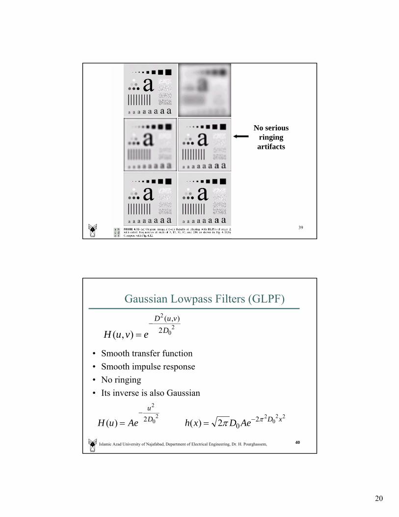
39
No serious ringing artifacts
Islamic Azad University of Najafabad, Department of Electrical Engineering, Dr. H. Pourghassem, 40
• Smooth transfer function• Smooth impulse response• No ringing• Its inverse is also Gaussian
20
2
2),(
),( DvuD
evuH−
=
Gaussian Lowpass Filters (GLPF)
220
220
2
20
2 2)()( xDDu
AeDxhAeuH ππ −−
==

21
Islamic Azad University of Najafabad, Department of Electrical Engineering, Dr. H. Pourghassem, 41
Gaussian Lowpass Filters (GLPF)
42
No serious ringing artifacts
22
Islamic Azad University of Najafabad, Department of Electrical Engineering, Dr. H. Pourghassem, 43
Islamic Azad University of Najafabad, Department of Electrical Engineering, Dr. H. Pourghassem, 44
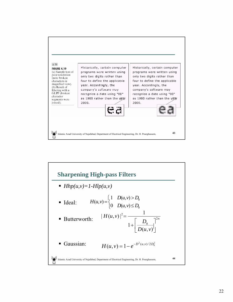
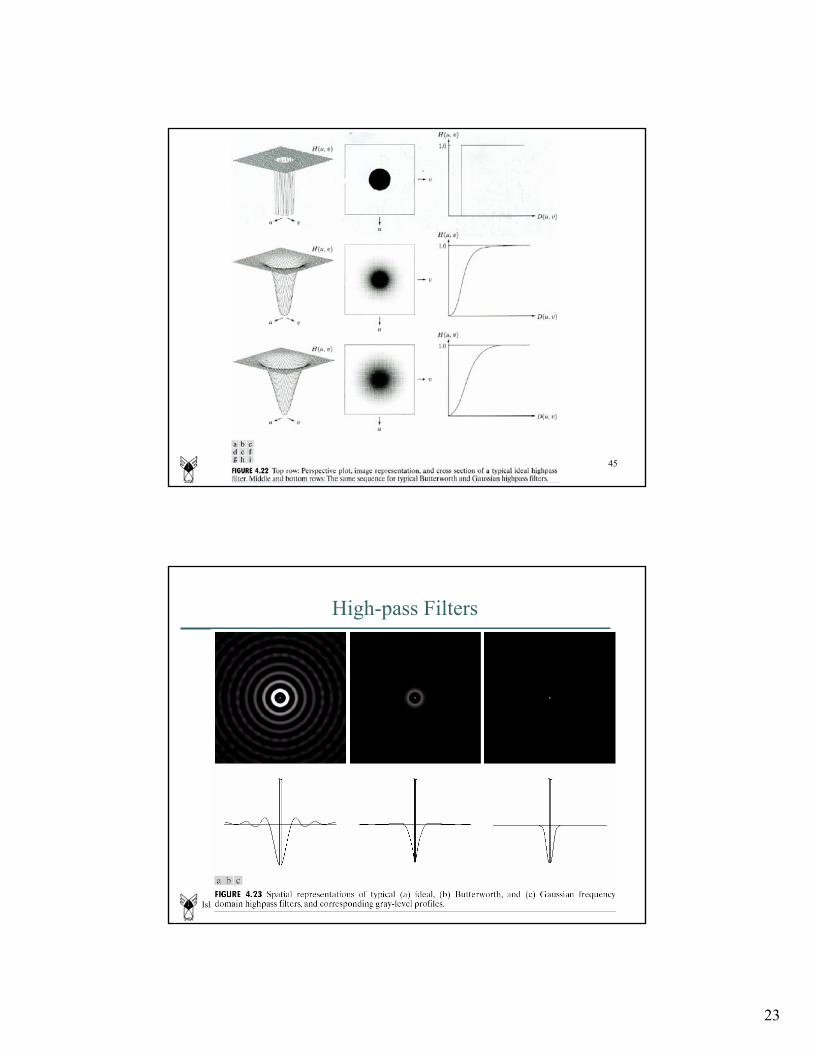
Sharpening High-pass Filters
Hhp(u,v)=1-Hlp(u,v)
Ideal:
Butterworth:
Gaussian:
n
vuDD
vuH 20
2
),(1
1|),(|
⎥⎦
⎤⎢⎣
⎡+
=
⎩⎨⎧
≤>
=0
0
),(0),(1
),(DvuDDvuD
vuH
20
2 2/),(1),( DvuDevuH −−=
23
45
Islamic Azad University of Najafabad, Department of Electrical Engineering, Dr. H. Pourghassem, 46
High-pass Filters

24
Islamic Azad University of Najafabad, Department of Electrical Engineering, Dr. H. Pourghassem, 47
Ideal High-pass Filtering
ringing artifacts
Islamic Azad University of Najafabad, Department of Electrical Engineering, Dr. H. Pourghassem, 48
Butterworth High-pass Filtering

25
Islamic Azad University of Najafabad, Department of Electrical Engineering, Dr. H. Pourghassem, 49
Gaussian High-pass Filtering
Islamic Azad University of Najafabad, Department of Electrical Engineering, Dr. H. Pourghassem, 50
Laplacian
∇2 f =∂ 2 f∂x 2 +
∂ 2 f∂y 2
∂ 2 f∂ 2x 2 = f (x +1, y) + f (x −1, y) − 2 f (x, y)
∂ 2 f∂ 2y 2 = f (x,y +1) + f (x,y −1) − 2 f (x, y)
∇2 f = [ f (x +1,y) + f (x −1,y) + f (x,y +1) + f (x,y −1)]− 4 f (x,y)

26
Islamic Azad University of Najafabad, Department of Electrical Engineering, Dr. H. Pourghassem, 51
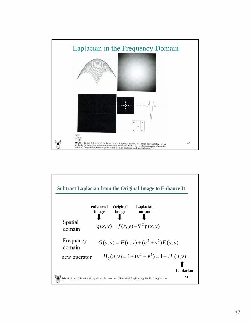
Laplacian in the Frequency Domain
),()(),(
),()(),(
vuFjvy
yxf
vuFjux
yxf
nn
n
nn
n
=⎥⎦
⎤⎢⎣
⎡∂
∂ℑ
=⎥⎦
⎤⎢⎣
⎡∂
∂ℑ
It can be shown
[ ] ),()(),( 222 vuFvuyxf +−=∇ℑ
Islamic Azad University of Najafabad, Department of Electrical Engineering, Dr. H. Pourghassem, 52
The Laplacian can be implemented in the FD by using the filter
FT pair:
Laplacian in the Frequency Domain
)(),( 22 vuvuH +−=
),(])2/()2/[(),( 222 vuFNvMuyxf −+−−⇔∇
27
53
Laplacian in the Frequency Domain
Islamic Azad University of Najafabad, Department of Electrical Engineering, Dr. H. Pourghassem, 54
Subtract Laplacian from the Original Image to Enhance It
),()(),(),( 22 vuFvuvuFvuG ++=
new operator
Spatial domain
Original image
enhanced image
Laplacian output
Frequency domain
Laplacian
),(1)(1),( 122
2 vuHvuvuH −=++=
),(),(),( 2 yxfyxfyxg ∇−=

28
55
Image Enhancement in the Frequency Domain
Islamic Azad University of Najafabad, Department of Electrical Engineering, Dr. H. Pourghassem, 56
Unsharp Masking, High-boost Filtering
Unsharp masking: fhp(x,y)=f(x,y)-flp(x,y)Hhp(u,v)=1-Hlp(u,v)
High-boost filtering: fhb(x,y)=Af(x,y)-flp(x,y)fhb(x,y)=(A-1)f(x,y)+fhp(x,y)Hhb(u,v)=(A-1)+Hhp(u,v)Hhfe(u,v)=a+bHhp(u,v)
One more parameter to
adjust the enhancement
High frequency emphasis

29
Islamic Azad University of Najafabad, Department of Electrical Engineering, Dr. H. Pourghassem, 57
Image Enhancement in Frequency Domain
Islamic Azad University of Najafabad, Department of Electrical Engineering, Dr. H. Pourghassem, 58
An image formation modelWe can view an image f(x,y) as a product of two components:
i(x,y): illumination. It is determined by the illumination source.r(x,y): reflectance. It is determined by the characteristics of imaged objects.
( ) ( ) ( )
1),(0),(0
,,,
<<∞<<
⋅=
yxryxi
yxryxiyxf

30
Islamic Azad University of Najafabad, Department of Electrical Engineering, Dr. H. Pourghassem, 59
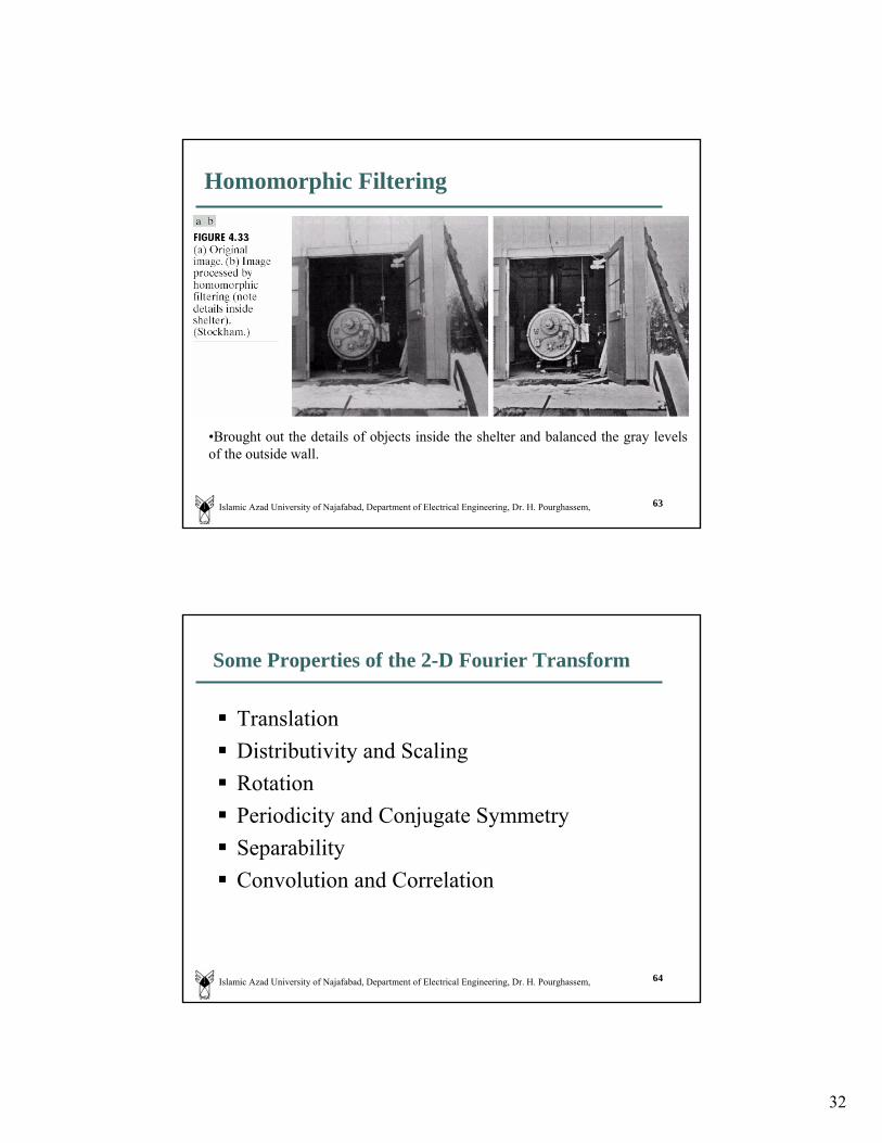
Homomorphic Filtering
In some images, the quality of the image has reduced because of non-uniform illumination.Homomorphic filtering can be used to perform illumination correction.
The above equation cannot be used directly in order to operate separately on the frequency components of illumination and reflectance.
( ) ( ) ( )yxryxiyxf ,,, ⋅=
Islamic Azad University of Najafabad, Department of Electrical Engineering, Dr. H. Pourghassem, 60
( ) ( ) ( )vuFvuFvuZ ri ,,, +=
( ) ( ) ( ) ( )yxryxiyxfyxz ,ln,ln,ln, +==
),(),(),(),(),(),(
00),(
''
yxryxieyxgyxryxiyxs
yxs ==
+=
Homomorphic Filtering
( )vuZvuHvuS ,),(),( =
ln :
DFT :
H(u,v) :
(DFT)-1 :
exp :

31
Islamic Azad University of Najafabad, Department of Electrical Engineering, Dr. H. Pourghassem, 61
By separating the illumination and reflectance components, homomorphic filter can then operate on them separately.Illumination component of an image generally has slow variations, while the reflectance component vary abruptly. By removing the low frequencies (highpass filtering) the effects of illumination can be removed .
Homomorphic Filtering
Islamic Azad University of Najafabad, Department of Electrical Engineering, Dr. H. Pourghassem, 62
Homomorphic Filtering
32
Islamic Azad University of Najafabad, Department of Electrical Engineering, Dr. H. Pourghassem, 63
Homomorphic Filtering
•Brought out the details of objects inside the shelter and balanced the gray levels of the outside wall.
Islamic Azad University of Najafabad, Department of Electrical Engineering, Dr. H. Pourghassem, 64
Some Properties of the 2-D Fourier Transform
TranslationDistributivity and ScalingRotationPeriodicity and Conjugate SymmetrySeparabilityConvolution and Correlation
33
Islamic Azad University of Najafabad, Department of Electrical Engineering, Dr. H. Pourghassem, 65
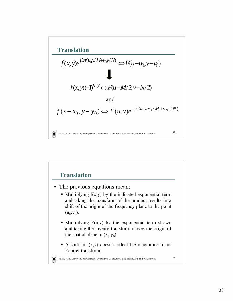
Translation
),(),( 00)//(2 00 vvuuFeyxf NyvMxuj −−⇔+π
)//(200
00),(),( NvyMuxjevuFyyxxf +−⇔−− π
and
)2/,2/()1)(,( NvMuFyxf yx −−⇔− +
Islamic Azad University of Najafabad, Department of Electrical Engineering, Dr. H. Pourghassem, 66
Translation
The previous equations mean:Multiplying f(x,y) by the indicated exponential term and taking the transform of the product results in a shift of the origin of the frequency plane to the point (u0,v0).
Multiplying F(u,v) by the exponential term shown and taking the inverse transform moves the origin of the spatial plane to (x0,y0).
A shift in f(x,y) doesn’t affect the magnitude of its Fourier transform.

34
Islamic Azad University of Najafabad, Department of Electrical Engineering, Dr. H. Pourghassem, 67
Distributivity and ScalingDistributive over addition but not over multiplication.
),(),( vuaFyxaf ⇔
)},({)},({)},(),({ 2121 yxfyxfyxfyxf ℑ+ℑ=+ℑ
)},({)},({)},(),({ 2121 yxfyxfyxfyxf ℑ⋅ℑ≠⋅ℑ
For two scalars a and b,
)/,/(1),( bvauFab
byaxf ⇔
Islamic Azad University of Najafabad, Department of Electrical Engineering, Dr. H. Pourghassem, 68
Rotation
Polar coordinates:
Which means that:
),(),,( become ),(),,( ϕωθ FrfvuFyxf
ϕϕθθ sincossincos wvwuryrx ====
35
Islamic Azad University of Najafabad, Department of Electrical Engineering, Dr. H. Pourghassem, 69
Rotation
Which means that rotating f(x,y) by an angle θ, rotates F(u,v) by the same angle (and vice versa).
),(),( 00 θϕωθθ +⇔+ Frf
Islamic Azad University of Najafabad, Department of Electrical Engineering, Dr. H. Pourghassem, 70
Periodicity & Conjugate Symmetry
The discrete FT and its inverse are periodic with period N:
),(),(),(),( NvMuFNvuFvMuFvuF ++=+=+=
For real f(x,y), FT also exhibits conjugate symmetry:
or),(),(),(),( *
vuFvuFvuFvuF
−−=
−−=

36
Islamic Azad University of Najafabad, Department of Electrical Engineering, Dr. H. Pourghassem, 71
Periodicity & Conjugate Symmetry
Islamic Azad University of Najafabad, Department of Electrical Engineering, Dr. H. Pourghassem, 72
SeparabilityThe discrete FT pair can be expressed in separable forms which (after some manipulations) can be expressed as:
F(u,v) =1M
F(x,v)exp[− j2πux / M]x= 0
M −1
∑
Where: F(x,v) =1N
f (x, y)exp[− j2πvy /N]y= 0
N−1
∑⎡
⎣ ⎢ ⎢
⎤
⎦ ⎥ ⎥

37
Islamic Azad University of Najafabad, Department of Electrical Engineering, Dr. H. Pourghassem, 73
Separability
The discrete FT pair can be expressed in separable forms which can be expressed as:
∑
∑ ∑−
=
−
=
−
=
−=
−−=
1
0
1
0
1
0
]/2exp[),(1),(
]/2exp[),(1]/2exp[1),(
M
x
M
x
M
y
MuxjvxFM
vuF
MvyjyxfN
MuxjM
vuF
π
ππ
Where: F(x,v) =1N
f (x, y)exp[− j2πvy /N]y= 0
N−1
∑⎡
⎣ ⎢ ⎢
⎤
⎦ ⎥ ⎥
Islamic Azad University of Najafabad, Department of Electrical Engineering, Dr. H. Pourghassem, 74
Convolution
Convolution theorem with FT pair:
),(),(),(*),( vuGvuFyxgyxf ⇔
),(*),(),(),( vuGvuFyxgyxf ⇔
H(u,v)vuFMN
y)f(x,y)h(x,
H(u,v)vuF,y)f(x,y)*h(x
*),(1),(
⇔
⇔
Convolution theorem with FT pair: (Matlab)

38
75
Periodicity: the Need for Padding
76
Periodicity: the Need for Padding

39
Islamic Azad University of Najafabad, Department of Electrical Engineering, Dr. H. Pourghassem, 77
Periodicity: the Need for Padding
• For convolution or correlation of two images f(x,y) and h(x,y) of sizes A*B and C*D, Wraparound error is avoided if we create images with the size of P*Q using following equation:
⎩⎨⎧
≤≤≤≤−≤≤−≤≤
=
⎩⎨⎧
≤≤≤≤−≤≤−≤≤
=
QyDorPxCDyandCxyxh
yxh
QyBorPxAByandAxyxf
yxf
e
e
01010),(
),(
01010),(
),(
11
−+≥−+≥
DBQCAP
Islamic Azad University of Najafabad, Department of Electrical Engineering, Dr. H. Pourghassem, 78
Correlation (Cross correlation)
Correlation of two functions f(x,y) and g(x,y):
),(),(),(),(*),(),(*),(),(
vuGvuFyxgyxfvuGvuFyxgyxf
οο
⇔⇔
Fourier Transform and Correlation:
∑∑−
=
−
=
++
=1
0
1
0
* ),(),(1),(),(
M
m
N
nnymxgnmf
MN
yxgyxf ο
40
Islamic Azad University of Najafabad, Department of Electrical Engineering, Dr. H. Pourghassem, 79
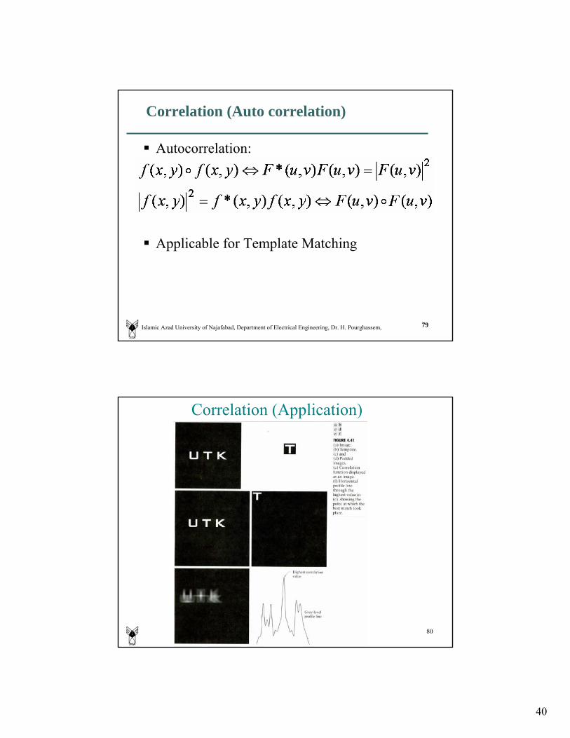
Correlation (Auto correlation)
Autocorrelation:
Applicable for Template Matching
80
Correlation (Application)