First-Order Probabilistic Languages: Into the Unknown
Brian Milch and Stuart RussellUniversity of California at Berkeley, USA
August 27, 2006
Based on joint work with Bhaskara Marthi, David Sontag, Andrey Kolobov, Daniel L. Ong

Knowledge Representation
deterministic
probabilistic
atomic propositional first-order
histogram17th–18th centuries
Probabilistic logic [Nilsson 1986],Graphical modelslate 20th century
Boolean logic19th century
First-order logic19th - early 20th century
First-order probabilistic languages (FOPLs)20th-21st centuries
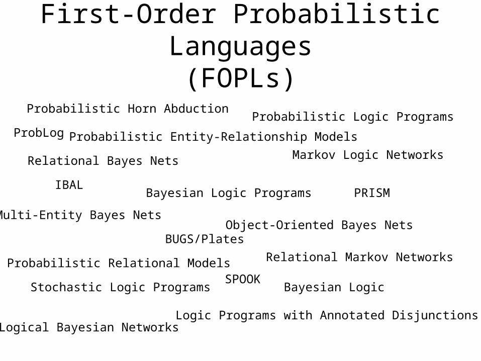
First-Order Probabilistic Languages(FOPLs)
Probabilistic Horn Abduction
Bayesian Logic Programs
Probabilistic Logic Programs
Relational Bayes Nets
BUGS/Plates
Probabilistic Relational Models
Markov Logic Networks
Relational Markov Networks
Bayesian Logic
Multi-Entity Bayes Nets
PRISM
Stochastic Logic Programs
Probabilistic Entity-Relationship Models
Object-Oriented Bayes Nets
IBAL
SPOOK
Logic Programs with Annotated DisjunctionsLogical Bayesian Networks
ProbLog
This Talk
• Taxonomy of FOPLs
• Design of a FOPL: Bayesian logic (BLOG)
• Inference in infinite Bayes nets
• Open problems in structure learning

S. Russel and P. Norvig (1995). Artificial Intelligence: A Modern Approach. Upper Saddle River, NJ: Prentice Hall.
Motivating Problem: Bibliographies
Russell, Stuart and Norvig, Peter. Articial Intelligence. Prentice-Hall, 1995.
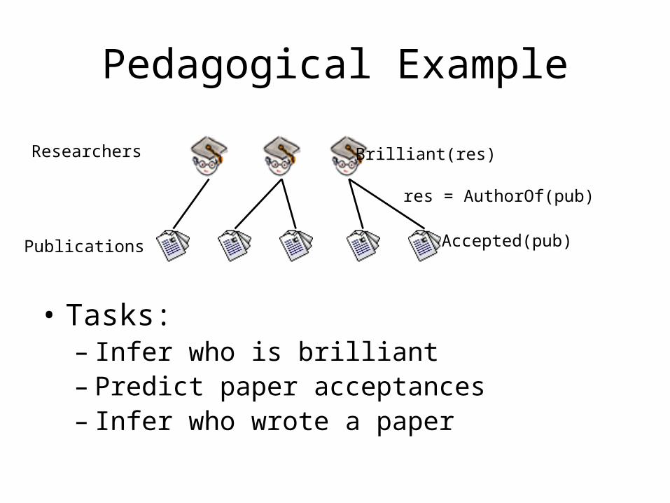
Pedagogical Example
• Tasks:– Infer who is brilliant– Predict paper acceptances– Infer who wrote a paper
res = AuthorOf(pub)
Researchers
Publications Accepted(pub)
Brilliant(res)
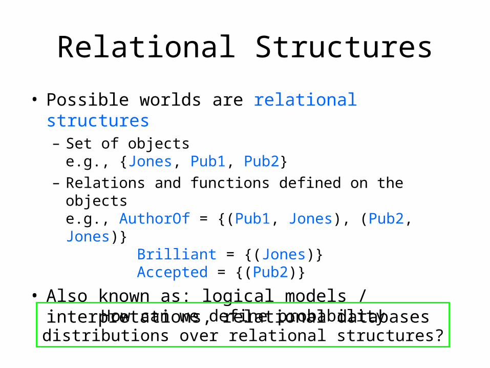
Relational Structures
• Possible worlds are relational structures – Set of objects
e.g., {Jones, Pub1, Pub2}– Relations and functions defined on the objects
e.g., AuthorOf = {(Pub1, Jones), (Pub2, Jones)} Brilliant = {(Jones)} Accepted = {(Pub2)}
• Also known as: logical models / interpretations, relational databases
How can we define probability distributions over relational structures?

Taxonomy of FOPLs, first level
Outcome Space
Relationalstructures
Proofs (and hence logical atoms)
Nested datastructures
SLPs [Muggleton 1996]
IBAL [Pfeffer 2001]
Instantiations of randomvariables
Early KBMCBUGS/Plates [Gilks et al. 1994]BLPs [Kersting & De Raedt 2001]
First-orderinterpretations
Relationaldatabases
PRMs [Koller & Pfeffer 1998]RMNs [Taskar et al. 2002]DAPER models [Heckerman et al. 2004]
PHA [Poole 1992]RBNs [Jaeger 1997]PRISM [Sato 1997]MLNs [Domingos & Richardson 2004]BLOG [Milch et al. 2004]...
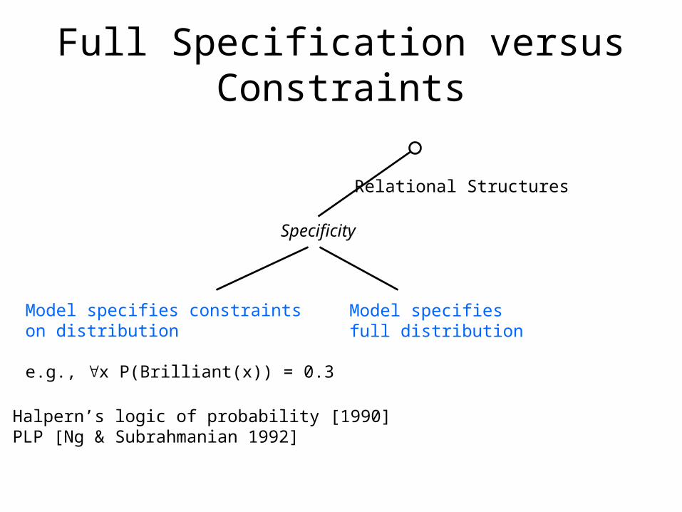
Full Specification versus Constraints
Specificity
Model specifies constraints on distribution e.g., x P(Brilliant(x)) = 0.3
Model specifies full distribution
Halpern’s logic of probability [1990]PLP [Ng & Subrahmanian 1992]
Relational Structures
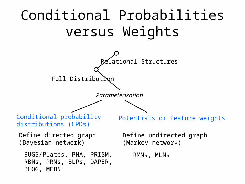
Conditional Probabilities versus Weights
Parameterization
Conditional probability distributions (CPDs)
Potentials or feature weights
RMNs, MLNsBUGS/Plates, PHA, PRISM, RBNs, PRMs, BLPs, DAPER, BLOG, MEBN
Relational Structures
Full Distribution
Define directed graph (Bayesian network)
Define undirected graph (Markov network)
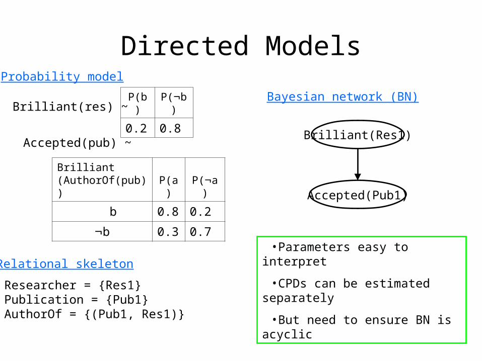
Directed Models
Brilliant(AuthorOf(pub)) P(a) P(a)
b 0.8 0.2
b 0.3 0.7
P(b) P(b)
0.2 0.8Brilliant(res) ~
Accepted(pub) ~Brilliant(Res1)
Accepted(Pub1)
Probability model
Relational skeleton
Researcher = {Res1}Publication = {Pub1}AuthorOf = {(Pub1, Res1)}
Bayesian network (BN)
•Parameters easy to interpret
•CPDs can be estimated separately
•But need to ensure BN is acyclic
•Parameters easy to interpret
•CPDs can be estimated separately
•But need to ensure BN is acyclic
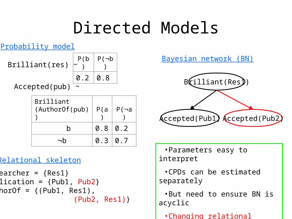
Directed Models
Brilliant(AuthorOf(pub)) P(a) P(a)
b 0.8 0.2
b 0.3 0.7
P(b) P(b)
0.2 0.8Brilliant(res) ~
Accepted(pub) ~Brilliant(Res1)
Accepted(Pub1)
Probability model
Relational skeleton
Researcher = {Res1}Publication = {Pub1, Pub2}AuthorOf = {(Pub1, Res1), (Pub2, Res1)}
Bayesian network (BN)
•Parameters easy to interpret
•CPDs can be estimated separately
•But need to ensure BN is acyclic
•Changing relational skeleton doesn’t change optimal parameters
Accepted(Pub2)
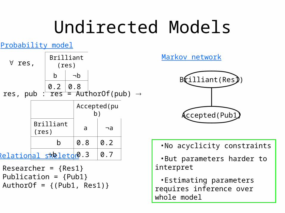
Undirected ModelsProbability model
Relational skeleton
Markov network
res, pub : res = AuthorOf(pub)
Researcher = {Res1}Publication = {Pub1}AuthorOf = {(Pub1, Res1)}
Brilliant(Res1)
Accepted(Pub1)
•No acyclicity constraints
•But parameters harder to interpret
•Estimating parameters requires inference over whole model
Accepted(pub)
Brilliant(res) a a
b 0.8 0.2
b 0.3 0.7
Brilliant(res)
b b
0.2 0.8
res,
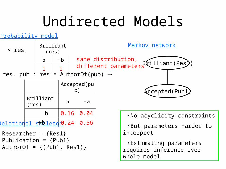
Undirected ModelsProbability model
Relational skeleton
Markov network
res, pub : res = AuthorOf(pub)
Researcher = {Res1}Publication = {Pub1}AuthorOf = {(Pub1, Res1)}
Brilliant(Res1)
Accepted(Pub1)
•No acyclicity constraints
•But parameters harder to interpret
•Estimating parameters requires inference over whole model
Accepted(pub)
Brilliant(res) a a
b 0.16 0.04
b 0.24 0.56
Brilliant(res)
b b
1 1
res,
same distribution, different parameters

•No acyclicity constraints
•But parameters harder to interpret
•Estimating parameters requires inference over whole model
Researcher = {Res1}Publication = {Pub1, Pub2}AuthorOf = {(Pub1, Res1), (Pub2, Res1)}
Undirected ModelsProbability model
Relational skeleton
Markov network
res, pub : res = AuthorOf(pub)
Brilliant(Res1)
Accepted(Pub1)
•No acyclicity constraints
•But parameters harder to interpret
•Estimating parameters requires inference over whole model
•Changing relational skeleton may change optimality of parameters
Accepted(pub)
Brilliant(res) a a
b 0.16 0.04
b 0.24 0.56
Brilliant(res)
b b
1 1
res,
Accepted(Pub2)
marginal now [(0.2)2, (0.8)2]
appliestwice
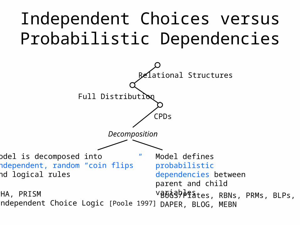
Independent Choices versus Probabilistic Dependencies
Decomposition
Model is decomposed into independent, random “coin flips”and logical rules
Model defines probabilistic dependencies between parent and child variables
PHA, PRISMIndependent Choice Logic [Poole 1997]
BUGS/Plates, RBNs, PRMs, BLPs, DAPER, BLOG, MEBN
CPDs
Relational Structures
Full Distribution
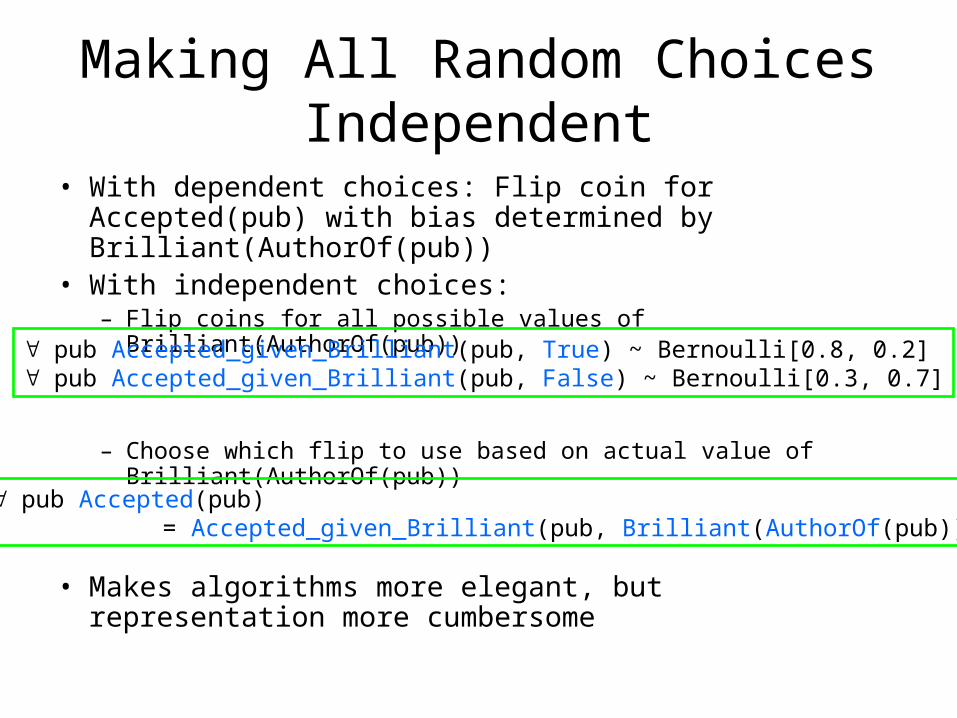
• With dependent choices: Flip coin for Accepted(pub) with bias determined by Brilliant(AuthorOf(pub))
• With independent choices: – Flip coins for all possible values of Brilliant(AuthorOf(pub))
– Choose which flip to use based on actual value of Brilliant(AuthorOf(pub))
• Makes algorithms more elegant, but representation more cumbersome
Making All Random Choices Independent
pub Accepted_given_Brilliant(pub, True) ~ Bernoulli[0.8, 0.2] pub Accepted_given_Brilliant(pub, False) ~ Bernoulli[0.3, 0.7]
pub Accepted(pub) = Accepted_given_Brilliant(pub, Brilliant(AuthorOf(pub)))
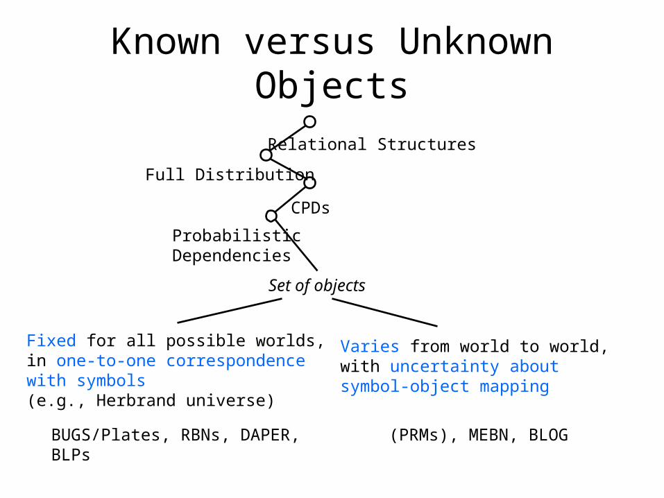
Known versus Unknown Objects
Set of objects
Fixed for all possible worlds,in one-to-one correspondencewith symbols(e.g., Herbrand universe)
Varies from world to world, with uncertainty about symbol-object mapping
BUGS/Plates, RBNs, DAPER, BLPs
(PRMs), MEBN, BLOG
CPDs
Relational Structures
Full Distribution
ProbabilisticDependencies
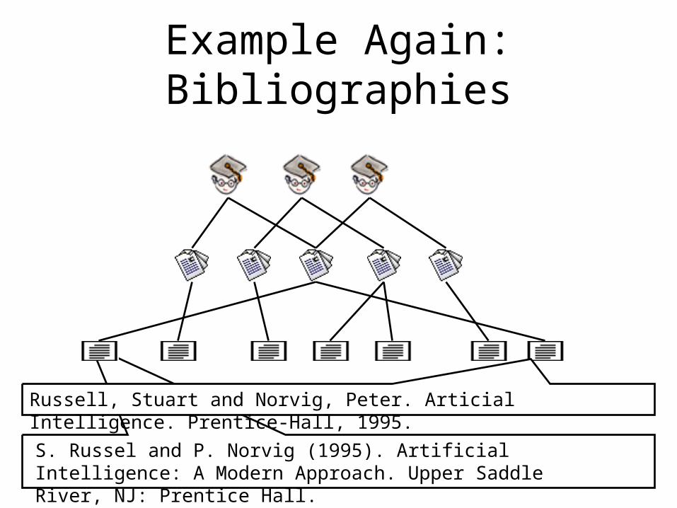
S. Russel and P. Norvig (1995). Artificial Intelligence: A Modern Approach. Upper Saddle River, NJ: Prentice Hall.
Example Again: Bibliographies
Russell, Stuart and Norvig, Peter. Articial Intelligence. Prentice-Hall, 1995.

Levels of Uncertainty
A
CB
D
A
CB
D
A
CB
D
A
CB
D
AttributeUncertainty
A
CB
D
A
CB
D
A
CB
D
A
CB
D
RelationalUncertainty
A, C
B, D
UnknownObjects
A, B,C, D
A, C
B, D
A
C, DB
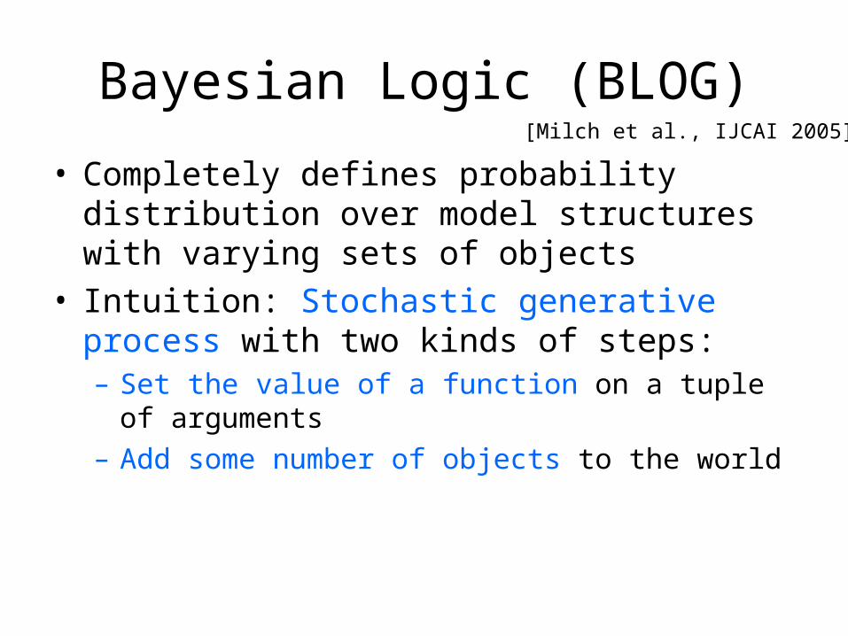
Bayesian Logic (BLOG)
• Completely defines probability distribution over model structures with varying sets of objects
• Intuition: Stochastic generative process with two kinds of steps:– Set the value of a function on a tuple of arguments– Add some number of objects to the world
[Milch et al., IJCAI 2005]
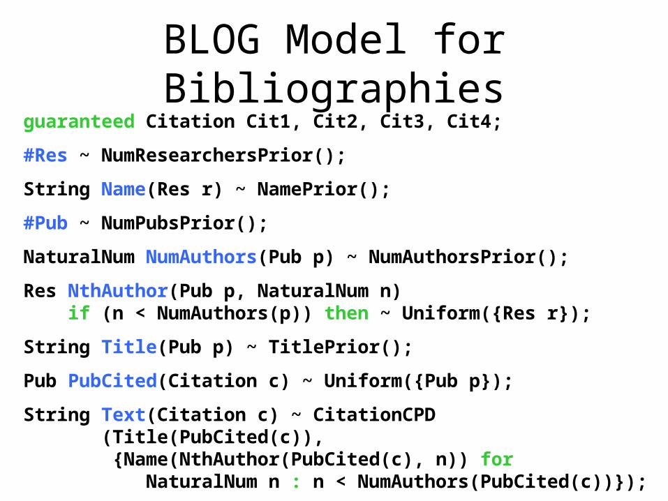
BLOG Model for Bibliographiesguaranteed Citation Cit1, Cit2, Cit3, Cit4;
#Res ~ NumResearchersPrior();
String Name(Res r) ~ NamePrior();
#Pub ~ NumPubsPrior();
NaturalNum NumAuthors(Pub p) ~ NumAuthorsPrior();
Res NthAuthor(Pub p, NaturalNum n) if (n < NumAuthors(p)) then ~ Uniform({Res r});
String Title(Pub p) ~ TitlePrior();
Pub PubCited(Citation c) ~ Uniform({Pub p});
String Text(Citation c) ~ CitationCPD (Title(PubCited(c)), {Name(NthAuthor(PubCited(c), n)) for NaturalNum n : n < NumAuthors(PubCited(c))});

guaranteed Citation Cit1, Cit2, Cit3, Cit4;
#Res ~ NumResearchersPrior();
String Name(Res r) ~ NamePrior();
#Pub ~ NumPubsPrior();
NaturalNum NumAuthors(Pub p) ~ NumAuthorsPrior();
Res NthAuthor(Pub p, NaturalNum n) if (n < NumAuthors(p)) then ~ Uniform({Res r});
String Title(Pub p) ~ TitlePrior();
Pub PubCited(Citation c) ~ Uniform({Pub p});
String Text(Citation c) ~ CitationCPD (Title(PubCited(c)), {Name(NthAuthor(PubCited(c), n)) for NaturalNum n : n < NumAuthors(PubCited(c))});
BLOG Model for Bibliographies
Number statements
Dependency statements
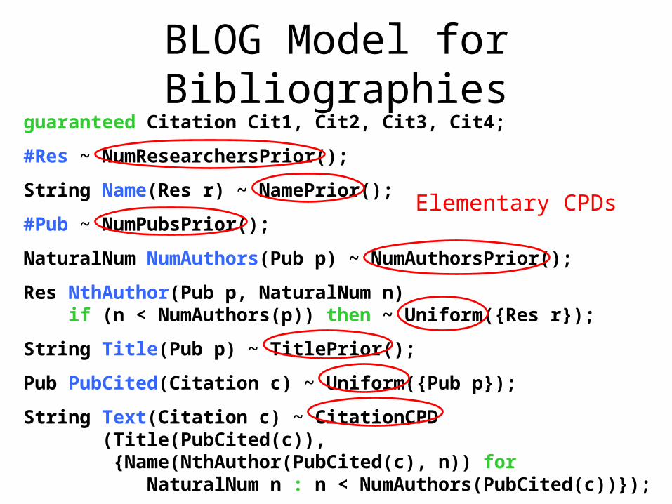
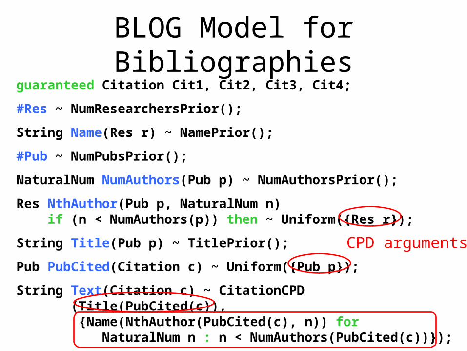
guaranteed Citation Cit1, Cit2, Cit3, Cit4;
#Res ~ NumResearchersPrior();
String Name(Res r) ~ NamePrior();
#Pub ~ NumPubsPrior();
NaturalNum NumAuthors(Pub p) ~ NumAuthorsPrior();
Res NthAuthor(Pub p, NaturalNum n) if (n < NumAuthors(p)) then ~ Uniform({Res r});
String Title(Pub p) ~ TitlePrior();
Pub PubCited(Citation c) ~ Uniform({Pub p});
String Text(Citation c) ~ CitationCPD (Title(PubCited(c)), {Name(NthAuthor(PubCited(c), n)) for NaturalNum n : n < NumAuthors(PubCited(c))});
BLOG Model for Bibliographies
Elementary CPDs
guaranteed Citation Cit1, Cit2, Cit3, Cit4;
#Res ~ NumResearchersPrior();
String Name(Res r) ~ NamePrior();
#Pub ~ NumPubsPrior();
NaturalNum NumAuthors(Pub p) ~ NumAuthorsPrior();
Res NthAuthor(Pub p, NaturalNum n) if (n < NumAuthors(p)) then ~ Uniform({Res r});
String Title(Pub p) ~ TitlePrior();
Pub PubCited(Citation c) ~ Uniform({Pub p});
String Text(Citation c) ~ CitationCPD (Title(PubCited(c)), {Name(NthAuthor(PubCited(c), n)) for NaturalNum n : n < NumAuthors(PubCited(c))});
BLOG Model for Bibliographies
CPD arguments
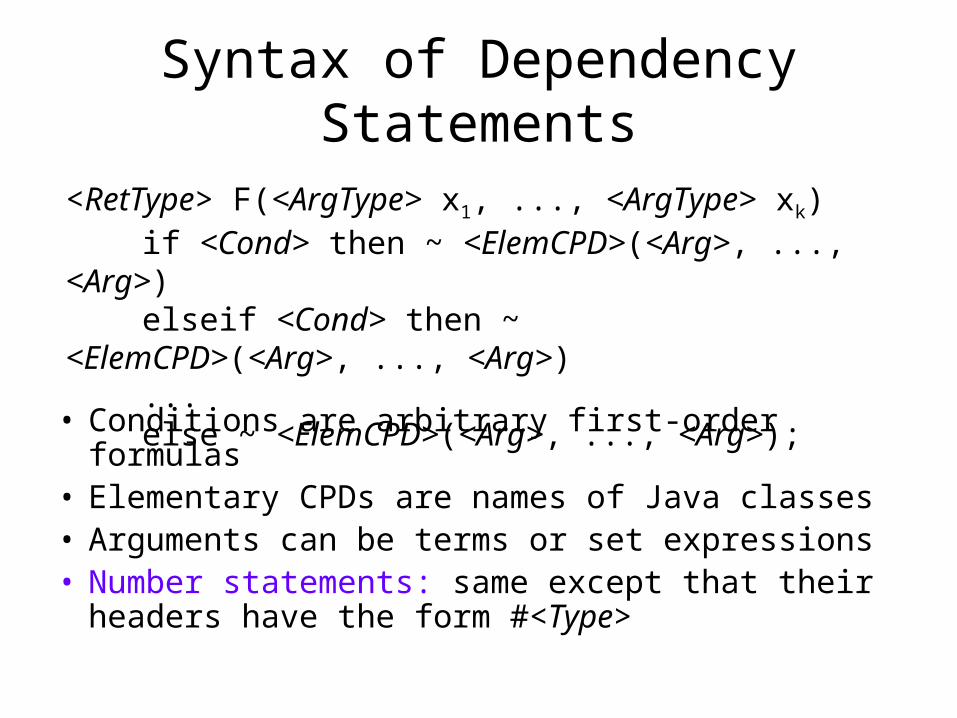
Syntax of Dependency Statements
<RetType> F(<ArgType> x1, ..., <ArgType> xk) if <Cond> then ~ <ElemCPD>(<Arg>, ..., <Arg>) elseif <Cond> then ~ <ElemCPD>(<Arg>, ..., <Arg>) ... else ~ <ElemCPD>(<Arg>, ..., <Arg>);
• Conditions are arbitrary first-order formulas• Elementary CPDs are names of Java classes• Arguments can be terms or set expressions• Number statements: same except that their
headers have the form #<Type>
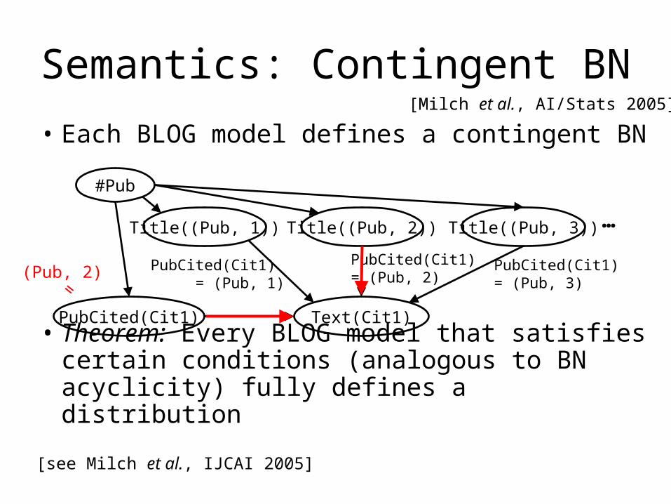
Semantics: Contingent BN
• Each BLOG model defines a contingent BN
• Theorem: Every BLOG model that satisfies certain conditions (analogous to BN acyclicity) fully defines a distribution
Title((Pub, 1)) Title((Pub, 2)) Title((Pub, 3)) …
Text(Cit1)PubCited(Cit1)
#Pub
PubCited(Cit1) = (Pub, 1)
PubCited(Cit1) = (Pub, 2)
PubCited(Cit1) = (Pub, 3)
[Milch et al., AI/Stats 2005]
[see Milch et al., IJCAI 2005]
(Pub, 2)=
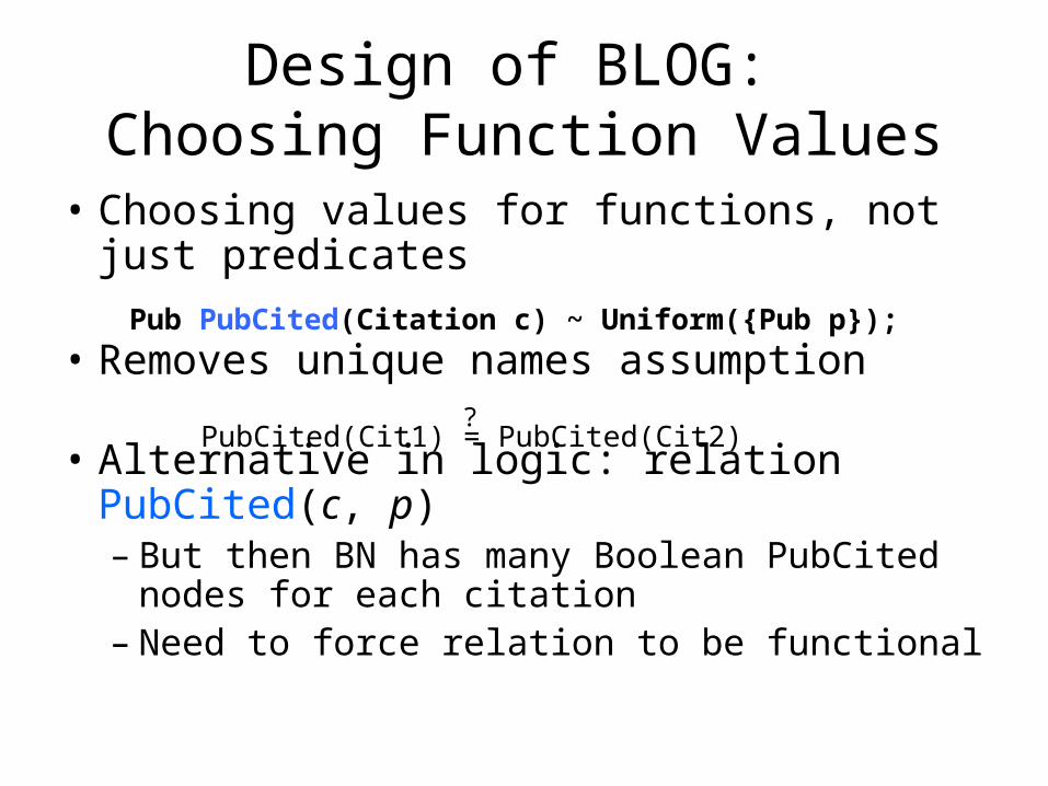
Design of BLOG: Choosing Function Values
• Choosing values for functions, not just predicates
• Removes unique names assumption
• Alternative in logic: relation PubCited(c, p)– But then BN has many Boolean PubCited
nodes for each citation– Need to force relation to be functional
Pub PubCited(Citation c) ~ Uniform({Pub p});
PubCited(Cit1) = PubCited(Cit2)?
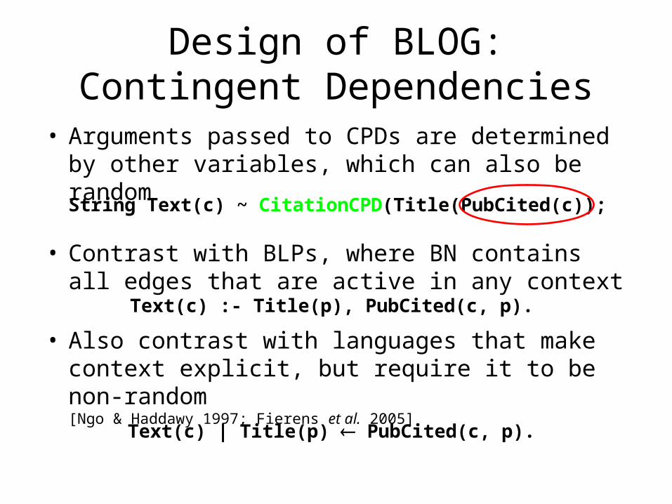
Design of BLOG:Contingent Dependencies
• Arguments passed to CPDs are determined by other variables, which can also be random
• Contrast with BLPs, where BN contains all edges that are active in any context
• Also contrast with languages that make context explicit, but require it to be non-random [Ngo & Haddawy 1997; Fierens et al. 2005]
String Text(c) ~ CitationCPD(Title(PubCited(c));
Text(c) :- Title(p), PubCited(c, p).
Text(c) | Title(p) PubCited(c, p).

Design of BLOG:Explicit Aggregation
• One dependency statement per random function– Can have if-then-else clauses
– Can pass multisets into CPDs
• Contrast with combining rules in BLPs, etc.
String Title(Pub p) if Type(p) = Proceedings then ~ ProcTitlePrior else ~ OrdinaryTitlePrior;
String Text(Citation c) ~ CitationCPD (Title(PubCited(c)), {Name(NthAuthor(PubCited(c), n)) for NaturalNum n : n < NumAuthors(PubCited(c))});

Design of BLOG:Number Statements
• Distribution for number of objects of a type– Can also have objects generating objects, e.g.,
aircraft generating radar blips
• Contrast with existence variables in MEBN [Laskey & Costa 2005]
– Easier to have one number variable than sequence of existence variables
– Number statements make interchangeability explicit• Can be exploited in inference; see [Milch & Russell, UAI ’06]
#Pub ~ NumPubsPrior();

Inference
• Task: Find posterior probability that query Q is true given evidence E
• Naive solution involves summing probabilities of worlds in E and in E Q
E
Q
)(
)()|(
EP
QEPEQP
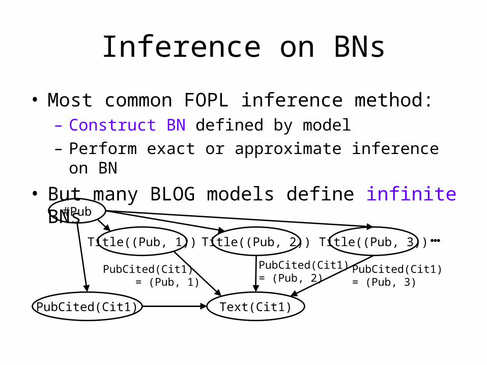
Inference on BNs
• Most common FOPL inference method:– Construct BN defined by model– Perform exact or approximate inference on BN
• But many BLOG models define infinite BNs
Title((Pub, 1)) Title((Pub, 2)) Title((Pub, 3)) …
Text(Cit1)PubCited(Cit1)
#Pub
PubCited(Cit1) = (Pub, 1)
PubCited(Cit1) = (Pub, 2)
PubCited(Cit1) = (Pub, 3)
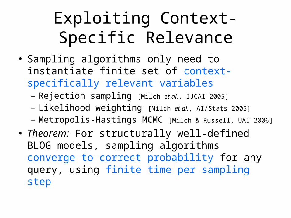
Exploiting Context-Specific Relevance
• Sampling algorithms only need to instantiate finite set of context-specifically relevant variables– Rejection sampling [Milch et al., IJCAI 2005]
– Likelihood weighting [Milch et al., AI/Stats 2005]
– Metropolis-Hastings MCMC [Milch & Russell, UAI 2006]
• Theorem: For structurally well-defined BLOG models, sampling algorithms converge to correct probability for any query, using finite time per sampling step

Metropolis-Hastings MCMC
• Let s1 be arbitrary state in E• For n = 1 to N
– Sample sE from proposal distribution q(s | sn)
– Compute acceptance probability
– With probability , let sn+1 = s;
else let sn+1 = sn
nn
n
ssqsp
ssqsp
|
|,1max
Fraction of visited states in Q converges to p(Q|E)
E
Q
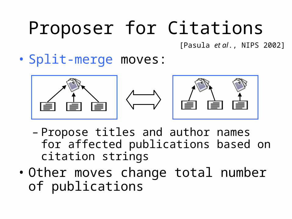
Proposer for Citations
• Split-merge moves:
– Propose titles and author names for affected publications based on citation strings
• Other moves change total number of publications
[Pasula et al., NIPS 2002]

MCMC States
• Not complete instantiations!– No titles, author names for uncited publications
• States are partial instantiations of random variables
– Each state corresponds to an event: set of worlds satisfying description
#Pub = 100, PubCited(Cit1) = (Pub, 37), Title((Pub, 37)) = “Calculus”
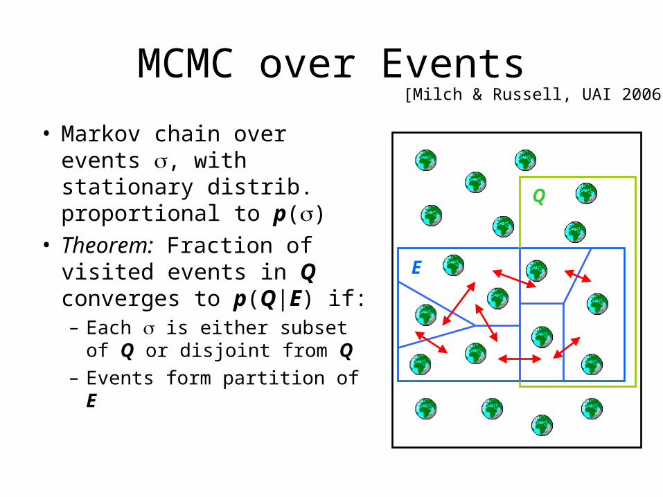
MCMC over Events
• Markov chain over events , with stationary distrib. proportional to p()
• Theorem: Fraction of visited events in Q converges to p(Q|E) if:– Each is either subset of Q
or disjoint from Q– Events form partition of E
E
Q
[Milch & Russell, UAI 2006]
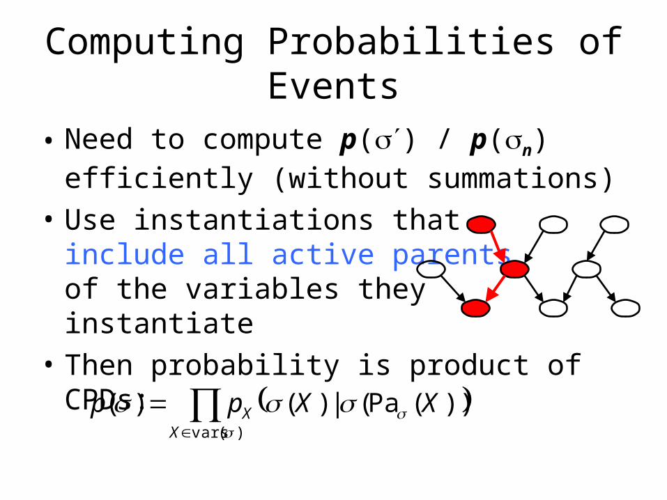
Computing Probabilities of Events
• Need to compute p() / p(n) efficiently (without summations)
• Use instantiations that include all active parents of the variables they instantiate
• Then probability is product of CPDs:
)(vars
))(Pa(|)()(
X
X XXpp

Learning
• Parameters: – Easy to estimate CPDs from complete data– With incomplete data, use EM algorithm
• Structure: – Choose parents [e.g., Friedman et al. 1999,
Popescul et al. 2003, Landwehr et al. 2005, Kok & Domingos 2005]
– Choose aggregation functions– Learn conditions under which CPDs apply
Predicate/Function Invention
• Predicate invention has long history in ILP– But typically new predicates are defined
deterministically in terms of existing predicates
• In probabilistic case: Invent random functions– With existing functions as parents, as in [Revoredo et
al., this conference]– Without parents, e.g., relation Colleagues(a, b) to
explain co-authorship patterns
• Inventing family of latent variables in BN

Entity Invention
• Invent new types of objects, such as:– Atoms (as in John McCarthy’s talk)– Conferences, to explain recurring substrings
of citation strings
• Requires representation that allows unknown objects– Objects of invented types will not be known to
modeler in advance
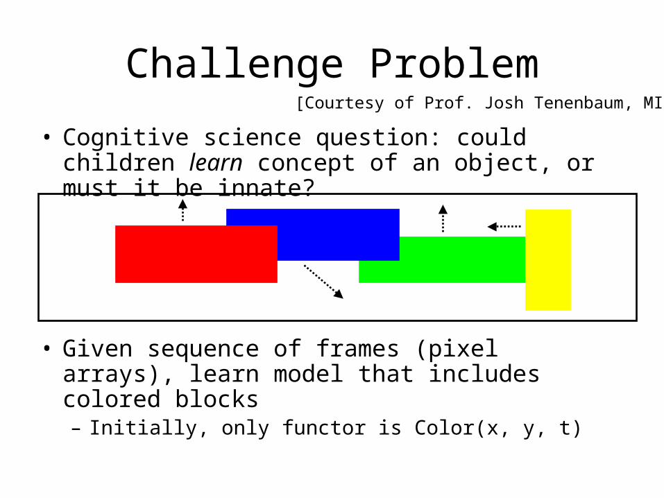
Challenge Problem
• Cognitive science question: could children learn concept of an object, or must it be innate?
• Given sequence of frames (pixel arrays), learn model that includes colored blocks– Initially, only functor is Color(x, y, t)
[Courtesy of Prof. Josh Tenenbaum, MIT]
Summary
• There is method to the madness of FOPLs• Bayesian logic (BLOG)
– Defines full distribution over relational structures– Allows unknown objects, unknown mapping from
symbols to objects– Makes contingent dependencies explicit
• Inference can be possible even when model yields infinite BN
• Exciting challenges in predicate/entity invention
http://www.cs.berkeley.edu/~milch/blog


![Probabilistic Logic Programming Languages · 2019. 3. 7. · 2.1.2 ProbLog The design of ProbLog [De Raedt et al., 2007] was motivated by the desire to make the simplest probabilistic](https://static.cupdf.com/doc/110x72/6141f0a52035ff3bc76259d7/probabilistic-logic-programming-languages-2019-3-7-212-problog-the-design.jpg)