FERRORESONANCE SIMULATION STUDIES
OF TRANSMISSION SYSTEMS
A thesis submitted to
THE UNIVERSITY OF MANCHESTER
for the degree of
DOCTOR OF PHILOSOPHY
in the Faculty of Engineering and Physical Sciences
2010
Swee Peng Ang
School of Electrical and Electronic Engineering
List of Contents
- 2 -
LIST OF CONTENTSLIST OF CONTENTSLIST OF CONTENTSLIST OF CONTENTS
LLL IIISSSTTT OOOFFF CCCOOONNNTTTEEENNNTTTSSS ... ... ... ... ... ... ... ... ... ... ... ... ... ... ... ... ... ... ... ... ... ... ... ... ... ... ... ... ... ... ... ... ... ... ... ... ... ... ... ... ... ... ... ... ... ... ... ... ... ... ... ... ... ... ... ... ... ... ... ... ... ... ... ... ... ... ... ... ... ... ... ... ... ... ... ... ... ... ... ... ... ... ... ... ... ... ... ... ... ... ... ... ... ... ... ... ... ... ... ... --- 222 ---
LLL IIISSSTTT OOOFFF FFFIIIGGGUUURRREEESSS... ... ... ... ... ... ... ... ... ... ... ... ... ... ... ... ... ... ... ... ... ... ... ... ... ... ... ... ... ... ... ... ... ... ... ... ... ... ... ... ... ... ... ... ... ... ... ... ... ... ... ... ... ... ... ... ... ... ... ... ... ... ... ... ... ... ... ... ... ... ... ... ... ... ... ... ... ... ... ... ... ... ... ... ... ... ... ... ... ... ... ... ... ... ... ... ... ... ... ... ... ... ... ... --- 555 ---
LLL IIISSSTTT OOOFFF TTTAAABBBLLL EEESSS ... ... ... ... ... ... ... ... ... ... ... ... ... ... ... ... ... ... ... ... ... ... ... ... ... ... ... ... ... ... ... ... ... ... ... ... ... ... ... ... ... ... ... ... ... ... ... ... ... ... ... ... ... ... ... ... ... ... ... ... ... ... ... ... ... ... ... ... ... ... ... ... ... ... ... ... ... ... ... ... ... ... ... ... ... ... ... ... ... ... ... ... ... ... ... ... ... ... ... ... ... ... ... --- 111000 ---
LLL IIISSSTTT OOOFFF PPPUUUBBBLLL IIICCCAAATTTIIIOOONNNSSS ... ... ... ... ... ... ... ... ... ... ... ... ... ... ... ... ... ... ... ... ... ... ... ... ... ... ... ... ... ... ... ... ... ... ... ... ... ... ... ... ... ... ... ... ... ... ... ... ... ... ... ... ... ... ... ... ... ... ... ... ... ... ... ... ... ... ... ... ... ... ... ... ... ... ... ... ... ... ... ... ... ... ... ... ... ... ... ... ... ... ... --- 111111 ---
AAABBB SSSTTTRRRAAACCCTTT ... ... ... ... ... ... ... ... ... ... ... ... ... ... ... ... ... ... ... ... ... ... ... ... ... ... ... ... ... ... ... ... ... ... ... ... ... ... ... ... ... ... ... ... ... ... ... ... ... ... ... ... ... ... ... ... ... ... ... ... ... ... ... ... ... ... ... ... ... ... ... ... ... ... ... ... ... ... ... ... ... ... ... ... ... ... ... ... ... ... ... ... ... ... ... ... ... ... ... ... ... ... ... ... ... ... ... ... ... ... ... ... --- 111222 ---
DDDEEECCCLLL AAARRRAAATTTIIIOOONNN ... ... ... ... ... ... ... ... ... ... ... ... ... ... ... ... ... ... ... ... ... ... ... ... ... ... ... ... ... ... ... ... ... ... ... ... ... ... ... ... ... ... ... ... ... ... ... ... ... ... ... ... ... ... ... ... ... ... ... ... ... ... ... ... ... ... ... ... ... ... ... ... ... ... ... ... ... ... ... ... ... ... ... ... ... ... ... ... ... ... ... ... ... ... ... ... ... ... ... ... ... ... ... ... ... ... --- 111333 ---
CCCOOOPPPYYY RRRIIIGGGHHHTTT SSSTTTAAATTTEEEMMMEEENNNTTT ... ... ... ... ... ... ... ... ... ... ... ... ... ... ... ... ... ... ... ... ... ... ... ... ... ... ... ... ... ... ... ... ... ... ... ... ... ... ... ... ... ... ... ... ... ... ... ... ... ... ... ... ... ... ... ... ... ... ... ... ... ... ... ... ... ... ... ... ... ... ... ... ... ... ... ... ... ... ... ... ... ... ... ... ... ... ... --- 111444 ---
AAACCCKKK NNNOOOWWWLLL EEEDDDGGGEEEMMMEEENNNTTT ... ... ... ... ... ... ... ... ... ... ... ... ... ... ... ... ... ... ... ... ... ... ... ... ... ... ... ... ... ... ... ... ... ... ... ... ... ... ... ... ... ... ... ... ... ... ... ... ... ... ... ... ... ... ... ... ... ... ... ... ... ... ... ... ... ... ... ... ... ... ... ... ... ... ... ... ... ... ... ... ... ... ... ... ... ... ... ... ... ... ... ... ... --- 111555 ---
CCCHHHAAAPPPTTTEEERRR 111 ... ... ... ... ... ... ... ... ... ... ... ... ... ... ... ... ... ... ... ... ... ... ... ... ... ... ... ... ... ... ... ... ... ... ... ... ... ... ... ... ... ... ... ... ... ... ... ... ... ... ... ... ... ... ... ... ... ... ... ... ... ... ... ... ... ... ... ... ... ... ... ... ... ... ... ... ... ... ... ... ... ... ... ... ... ... ... ... ... ... ... ... ... ... ... ... ... ... ... ... ... ... ... ... ... ... ... ... ... ... ... ... --- 111666 ---
111... IIINNNTTTRRROOODDDUUUCCCTTTIIIOOONNN ... ... ... ... ... ... ... ... ... ... ... ... ... ... ... ... ... ... ... ... ... ... ... ... ... ... ... ... ... ... ... ... ... ... ... ... ... ... ... ... ... ... ... ... ... ... ... ... ... ... ... ... ... ... ... ... ... ... ... ... ... ... ... ... ... ... ... ... ... ... ... ... ... ... ... ... ... ... ... ... ... ... ... ... ... ... ... ... ... ... ... ... ... ... ... --- 111666 ---
1.1 Introduction ..............................................................................................- 16 - 1.2 Background of Ferroresonance ................................................................- 17 - 1.3 Types of Ferroresonance Modes..............................................................- 20 -
1.3.1 Fundamental Mode ......................................................................- 20 - 1.3.2 Subharmonic Mode ......................................................................- 21 - 1.3.3 Quasi-periodic Mode ....................................................................- 22 - 1.3.4 Chaotic Mode...............................................................................- 22 -
1.4 Effect of Ferroresonance on Power Systems ...........................................- 27 - 1.5 Mitigation of Ferroresonance....................................................................- 28 - 1.6 Motivation.................................................................................................- 29 - 1.7 Methodology ............................................................................................- 30 - 1.8 Thesis structure........................................................................................- 32 -
CCCHHHAAAPPPTTTEEERRR 222 ... ... ... ... ... ... ... ... ... ... ... ... ... ... ... ... ... ... ... ... ... ... ... ... ... ... ... ... ... ... ... ... ... ... ... ... ... ... ... ... ... ... ... ... ... ... ... ... ... ... ... ... ... ... ... ... ... ... ... ... ... ... ... ... ... ... ... ... ... ... ... ... ... ... ... ... ... ... ... ... ... ... ... ... ... ... ... ... ... ... ... ... ... ... ... ... ... ... ... ... ... ... ... ... ... ... ... ... ... ... ... ... --- 333555 ---
222... LLL IIITTTEEERRRAAATTTUUURRREEE RRREEEVVVIIIEEEWWW ...... ... ... ... ... ... ... ... ... ... ... ... ... ... ... ... ... ... ... ... ... ... ... ... ... ... ... ... ... ... ... ... ... ... ... ... ... ... ... ... ... ... ... ... ... ... ... ... ... ... ... ... ... ... ... ... ... ... ... ... ... ... ... ... ... ... ... ... ... ... ... ... ... ... ... ... ... ... ... ... ... ... ... ... --- 333555 ---
2.1 Introduction ..............................................................................................- 35 - 2.2 Analytical Approach .................................................................................- 35 - 2.3 Analog Simulation Approach ....................................................................- 43 - 2.4 Real Field Test Approach.........................................................................- 49 - 2.5 Laboratory Measurement Approach .........................................................- 51 - 2.6 Digital Computer Program Approach........................................................- 55 - 2.7 Summary..................................................................................................- 60 -
CCCHHHAAAPPPTTTEEERRR 333 ... ... ... ... ... ... ... ... ... ... ... ... ... ... ... ... ... ... ... ... ... ... ... ... ... ... ... ... ... ... ... ... ... ... ... ... ... ... ... ... ... ... ... ... ... ... ... ... ... ... ... ... ... ... ... ... ... ... ... ... ... ... ... ... ... ... ... ... ... ... ... ... ... ... ... ... ... ... ... ... ... ... ... ... ... ... ... ... ... ... ... ... ... ... ... ... ... ... ... ... ... ... ... ... ... ... ... ... ... ... ... ... --- 666222 ---
333... SSSIIINNNGGGLLL EEE---PPPHHHAAASSSEEE FFFEEERRRRRROOORRREEESSSOOONNNAAANNNCCCEEE ––– AAA CCCAAASSSEEE SSSTTTUUUDDDYYY ... ... ... ... ... ... ... ... ... ... ... ... ... ... ... ... ... ... ... ... ... ... ... ... ... ... ... ... ... ... --- 666222 ---
3.1 Introduction ..............................................................................................- 62 - 3.2 Single-Phase Circuit Configuration...........................................................- 63 - 3.3 ATPDraw Model .......................................................................................- 65 - 3.4 Sensitivity Study on System Parameters..................................................- 67 -
3.4.1 Grading Capacitance (Cg) ............................................................- 68 - 3.4.2 Ground Capacitance (Cs) .............................................................- 69 - 3.4.3 Magnetising Resistance (Rm) .......................................................- 73 -
List of Contents
- 3 -
3.5 Influence of Core Nonlinearity on Ferroresonance................................... - 75 - 3.5.1 Grading Capacitance (Cg)............................................................ - 76 - 3.5.2 Ground Capacitance (Cs)............................................................. - 77 -
3.6 Comparison between Low and High Core Nonlinearity............................ - 81 - 3.7 Analysis and Discussion.......................................................................... - 82 - 3.8 Summary................................................................................................. - 87 -
CCCHHHAAAPPPTTTEEERRR 444 ... ... ... ... ... ... ... ... ... ... ... ... ... ... ... ... ... ... ... ... ... ... ... ... ... ... ... ... ... ... ... ... ... ... ... ... ... ... ... ... ... ... ... ... ... ... ... ... ... ... ... ... ... ... ... ... ... ... ... ... ... ... ... ... ... ... ... ... ... ... ... ... ... ... ... ... ... ... ... ... ... ... ... ... ... ... ... ... ... ... ... ... ... ... ... ... ... ... ... ... ... ... ... ... ... ... ... ... ... ... ... --- 888999 ---
444... SSSYYYSSSTTTEEEMMM CCCOOOMMMPPPOOONNNEEENNNTTT MMMOOODDDEEELLL SSS FFFOOORRR FFFEEERRRRRROOORRREEESSSOOONNNAAANNNCCCEEE ... ... ... ... ... ... ... ... ... ... ... ... ... ... ... ... ... ... ... ... ... ... ... --- 888999 ---
4.1 Introduction.............................................................................................. - 89 - 4.2 400-kV Circuit Breaker ............................................................................ - 89 - 4.3 Power Transformer.................................................................................. - 92 -
4.3.1 The Anhysteretic Curve ............................................................... - 93 - 4.3.2 Hysteresis Curve ......................................................................... - 99 - 4.3.3 Transformer models for ferroresonance study ........................... - 108 -
4.4 Transmission Line ................................................................................. - 119 - 4.4.1 Transmission Line Models in ATP-EMTP .................................. - 119 - 4.4.2 Literature Review of Transmission Line Model for Ferroresonance .... -
127 - 4.4.3 Handling of Simulation Time, ∆t................................................. - 128 -
4.4 Summary............................................................................................... - 131 -
CCCHHHAAAPPPTTTEEERRR 555 ... ... ... ... ... ... ... ... ... ... ... ... ... ... ... ... ... ... ... ... ... ... ... ... ... ... ... ... ... ... ... ... ... ... ... ... ... ... ... ... ... ... ... ... ... ... ... ... ... ... ... ... ... ... ... ... ... ... ... ... ... ... ... ... ... ... ... ... ... ... ... ... ... ... ... ... ... ... ... ... ... ... ... ... ... ... ... ... ... ... ... ... ... ... ... ... ... ... ... ... ... ... ... ... ... ... ... ... ... --- 111333333 ---
555... MMMOOODDDEEELLL IIINNNGGG OOOFFF 444000000 KKKVVV TTTHHHOOORRRPPPEEE--- MMMAAARRRSSSHHH///BBBRRRIIINNNSSSWWWOOORRRTTTHHH SSSYYYSSSTTTEEEMMM ...... ... ... ... ... ... ... ... ... --- 111333333 ---
5.1 Introduction............................................................................................ - 133 - 5.2 Description of the Transmission System................................................ - 133 - 5.3 Identification of the Origin of Ferroresonance Phenomenon .................. - 137 - 5.4 Modeling of the Transmission System ................................................... - 137 -
5.4.1 Modeling of the Circuit Breakers................................................ - 138 - 5.4.2 Modeling of 170 m Cable........................................................... - 141 - 5.4.3 Modeling of the Double-Circuit Transmission Line ..................... - 141 - 5.4.4 Modeling of Transformers SGT1 and SGT4............................... - 142 -
5.5 Simulation of the Transmission System................................................. - 145 - 5.5.1 Case Study 1: Transformer - BCTRAN+, Line - PI .................... - 145 - 5.5.2 Case Study 2: Transformer - BCTRAN+, Line - BERGERON... - 151 - 5.5.3 Case Study 3: Transformer - BCTRAN+, Line – MARTI ........... - 155 - 5.5.4 Case Study 4: Transformer - HYBRID, Line – PI ...................... - 161 - 5.5.5 Case Study 5: Transformer - HYBRID, Line – BERGERON ..... - 166 - 5.5.6 Case Study 6: Transformer - HYBRID, Line – MARTI............... - 170 -
5.6 Improvement of the Simulation Model.................................................... - 177 - 5.6.1 Selection of the Simulation Model.............................................. - 177 -
5.7 Key Parameters Influence the Occurrence of Ferroresonance .............. - 184 - 5.7.1 The Coupling Capacitances of the Power Transformer.............. - 185 - 5.7.2 The 170 m length Cable at the Secondary of the Transformer... - 186 - 5.7.3 The Transmission Line’s Coupling Capacitances....................... - 187 -
5.8 Summary............................................................................................... - 195 -
CCCHHHAAAPPPTTTEEERRR 666 ... ... ... ... ... ... ... ... ... ... ... ... ... ... ... ... ... ... ... ... ... ... ... ... ... ... ... ... ... ... ... ... ... ... ... ... ... ... ... ... ... ... ... ... ... ... ... ... ... ... ... ... ... ... ... ... ... ... ... ... ... ... ... ... ... ... ... ... ... ... ... ... ... ... ... ... ... ... ... ... ... ... ... ... ... ... ... ... ... ... ... ... ... ... ... ... ... ... ... ... ... ... ... ... ... ... ... ... ... --- 111999777 ---
666... MMMOOODDDEEELLL IIINNNGGG OOOFFF 444000000 KKKVVV IIIRRROOONNN---AAACCCTTTOOONNN///MMMEEELLL KKKSSSHHHAAAMMM SSSYYYSSSTTTEEEMMM...... ... ... ... ... ... ... ... ... ... ... ... ... ... ... ... ... ... ... ... ... --- 111999777 ---
6.1 Introduction............................................................................................ - 197 - 6.2 Description of the Transmission System................................................ - 197 -
List of Contents
- 4 -
6.3 Identify the Origin of Ferroresonance .....................................................- 199 - 6.4 Modeling the Iron-Acton/Melksham System ...........................................- 200 -
6.4.1 Modeling the Source Impedance and the Load ..........................- 200 - 6.4.2 Modeling the Circuit Breaker ......................................................- 201 - 6.4.3 Modeling the Cable ....................................................................- 202 - 6.4.4 Modeling the 33 km Double-Circuit Transmission Line ...............- 202 - 6.4.5 Modeling of Power Transformers SGT4 and SGT5 ....................- 203 -
6.5 Simulation Results of Iron-Acton/Melksham System ..............................- 207 - 6.6 Mitigation of Ferroresonance by Switch-in Shunt Reactor ......................- 211 - 6.7 Sensitivity Study of Double-Circuit Transmission Line ............................- 213 - 6.8 Summary................................................................................................- 217 -
CCCHHHAAAPPPTTTEEERRR 777 ... ... ... ... ... ... ... ... ... ... ... ... ... ... ... ... ... ... ... ... ... ... ... ... ... ... ... ... ... ... ... ... ... ... ... ... ... ... ... ... ... ... ... ... ... ... ... ... ... ... ... ... ... ... ... ... ... ... ... ... ... ... ... ... ... ... ... ... ... ... ... ... ... ... ... ... ... ... ... ... ... ... ... ... ... ... ... ... ... ... ... ... ... ... ... ... ... ... ... ... ... ... ... ... ... ... ... ... ... ... ... ... ... ... 222111888
777... CCCOOONNNCCCLLL UUUSSSIIIOOONNN AAANNNDDD FFFUUUTTTUUURRREEE WWWOOORRRKKK... ... ... ... ... ... ... ... ... ... ... ... ... ... ... ... ... ... ... ... ... ... ... ... ... ... ... ... ... ... ... ... ... ... ... ... ... ... ... ... ... ... ... ... ... ... ... ... ... ... ... ... ... ... ... ... ... ... ... ... ... ... ... ... ... 222111888
7.1 Conclusion .................................................................................................218 7.2 Future Work ...............................................................................................221
RRREEEFFFEEERRREEENNNCCCEEESSS ... ... ... ... ... ... ... ... ... ... ... ... ... ... ... ... ... ... ... ... ... ... ... ... ... ... ... ... ... ... ... ... ... ... ... ... ... ... ... ... ... ... ... ... ... ... ... ... ... ... ... ... ... ... ... ... ... ... ... ... ... ... ... ... ... ... ... ... ... ... ... ... ... ... ... ... ... ... ... ... ... ... ... ... ... ... ... ... ... ... ... ... ... ... ... ... ... ... ... ... ... ... ... ... ... ... ... ... ... ... 222222444
AAAPPPPPPEEENNNDDDIIIXXX AAA ... ... ... ... ... ... ... ... ... ... ... ... ... ... ... ... ... ... ... ... ... ... ... ... ... ... ... ... ... ... ... ... ... ... ... ... ... ... ... ... ... ... ... ... ... ... ... ... ... ... ... ... ... ... ... ... ... ... ... ... ... ... ... ... ... ... ... ... ... ... ... ... ... ... ... ... ... ... ... ... ... ... ... ... ... ... ... ... ... ... ... ... ... ... ... ... ... ... ... ... ... ... ... ... ... ... ... ... ... ... ... ... 222222999
AAAPPPPPPEEENNNDDDIIIXXX BBB ... ... ... ... ... ... ... ... ... ... ... ... ... ... ... ... ... ... ... ... ... ... ... ... ... ... ... ... ... ... ... ... ... ... ... ... ... ... ... ... ... ... ... ... ... ... ... ... ... ... ... ... ... ... ... ... ... ... ... ... ... ... ... ... ... ... ... ... ... ... ... ... ... ... ... ... ... ... ... ... ... ... ... ... ... ... ... ... ... ... ... ... ... ... ... ... ... ... ... ... ... ... ... ... ... ... ... ... ... ... ... ... 222333444
AAAPPPPPPEEENNNDDDIIIXXX CCC ... ... ... ... ... ... ... ... ... ... ... ... ... ... ... ... ... ... ... ... ... ... ... ... ... ... ... ... ... ... ... ... ... ... ... ... ... ... ... ... ... ... ... ... ... ... ... ... ... ... ... ... ... ... ... ... ... ... ... ... ... ... ... ... ... ... ... ... ... ... ... ... ... ... ... ... ... ... ... ... ... ... ... ... ... ... ... ... ... ... ... ... ... ... ... ... ... ... ... ... ... ... ... ... ... ... ... ... ... ... ... ... 222555999
AAAPPPPPPEEENNNDDDIIIXXX DDD ... ... ... ... ... ... ... ... ... ... ... ... ... ... ... ... ... ... ... ... ... ... ... ... ... ... ... ... ... ... ... ... ... ... ... ... ... ... ... ... ... ... ... ... ... ... ... ... ... ... ... ... ... ... ... ... ... ... ... ... ... ... ... ... ... ... ... ... ... ... ... ... ... ... ... ... ... ... ... ... ... ... ... ... ... ... ... ... ... ... ... ... ... ... ... ... ... ... ... ... ... ... ... ... ... ... ... ... ... ... ... ... 222666222
List of Figures
- 5 -
LIST OF FIGURESLIST OF FIGURESLIST OF FIGURESLIST OF FIGURES
CHAPTER 1: INTRODUCTION
Figure 1.1: Linear resonance circuit........................................................................... - 18 - Figure 1.2: Characteristic of Vc, VL, I and Es at resonance.......................................... - 18 - Figure 1.3: Ferroresonant circuit ................................................................................ - 19 - Figure 1.4: E-I characteristic of ferroresonance circuit ............................................... - 19 - Figure 1.5: Fundamental mode.................................................................................. - 21 - Figure 1.6: Subharmonic mode.................................................................................. - 21 - Figure 1.7: Quasi-periodic mode................................................................................ - 22 - Figure 1.8: Chaotic mode .......................................................................................... - 22 - Figure 1.9: Time signal .............................................................................................. - 23 - Figure 1.10: Power spectrum..................................................................................... - 23 - Figure 1.11: Poincarè plot.......................................................................................... - 23 - Figure 1.12: Phase-plane diagram............................................................................. - 24 - Figure 1.13: Time signal ............................................................................................ - 24 - Figure 1.14: Power spectrum..................................................................................... - 25 - Figure 1.15: Poincarè plot.......................................................................................... - 25 - Figure 1.16: Phase-plane diagram............................................................................. - 25 - Figure 1.17: Time signal ............................................................................................ - 26 - Figure 1.18: Power spectrum..................................................................................... - 26 - Figure 1.19: Poincarè plot.......................................................................................... - 26 - Figure 1.20: Phase-plane diagram............................................................................. - 26 - Figure 1.21: Outline of modeling methodology........................................................... - 31 -
CHAPTER 2: LITERATURE REVIEW
Figure 2.1: Section of a typical double-busbar 275 kV substation [12] ....................... - 36 - Figure 2.2: Section of a typical double-busbar 275 kV substation [11] ....................... - 36 - Figure 2.3: Model for ferroresonance circuit including line capacitance [25]............... - 37 - Figure 2.4: Circuit that feeds the disconnected coil [25] ............................................. - 37 - Figure 2.5: Basic ferroresonance circuit [25].............................................................. - 38 - Figure 2.6: Bifurcation diagrams- Top: n = 5, Bottom: n = 11 [23] ............................ - 39 - Figure 2.7: Distribution system of 4.16 kV essential bus at MNPS [24] ...................... - 40 - Figure 2.8: Island system at MNPS [24]..................................................................... - 41 - Figure 2.9: Ferroresonance condition - Island system at MNPS ................................ - 41 - Figure 2.10: Oscillogram at the MNPS 345 kV switchyard [24] .................................. - 42 - Figure 2.11: The Big Eddy and John Day transmission system [15]........................... - 44 - Figure 2.12: The Big Eddy/John Day system including coupling capacitances [15].... - 44 - Figure 2.13: Equivalent circuit of Big Eddy and John Day 525/241.5 kV system [15] . - 45 - Figure 2.14: Typical connection of potential transformer used in a ground-fault detector scheme on 3-phase 3-wire ungrounded power system [26]........................... - 46 - Figure 2.15: Anacom circuit to represent circuit of Figure 2.5 [26] ............................. - 46 - Figure 2.16: Possible ferroresonance circuit [27] ....................................................... - 47 - Figure 2.17: Three-phase equivalent system [28] ...................................................... - 48 - Figure 2.18: Subharmonic mode ferroresonance quenching [29]............................... - 50 - Figure 2.19: Fundamental mode ferroresonance quenching [29] ............................... - 50 - Figure 2.20: Laboratory setup [30] ............................................................................. - 51 - Figure 2.21: Transformer banks in series with capacitive impedance [31].................. - 53 - Figure 2.22: Transformers in series with capacitor (C3) for line model [31]................ - 53 - Figure 2.23: 400 kV line bay [13, 14] ......................................................................... - 55 -
List of Figures
- 6 -
Figure 2.24: ATPDraw representation of 400 kV substation [14].................................- 56 - Figure 2.25: Dorsey bus configuration prior to explosion of potential transformer [16] - 57 - Figure 2.26: Dorsey bus configuration with grading capacitors (Cg)............................- 58 - Figure 2.27: EMTP model – Main circuit components [16]..........................................- 58 - Figure 2.28: EMTP model – Bus model [16] ...............................................................- 59 - Figure 2.29: EMTP model – PT model [16].................................................................- 59 -
CHAPTER 3: SINGLE-PHASE FERRORESONANCE - A CASE STUDY
Figure 3.1: Single-phase ferroresonance circuit [16]...................................................- 63 - Figure 3.2: Magnetising characteristic [16] .................................................................- 64 - Figure 3.3: Core characteristic....................................................................................- 64 - Figure 3.4: ATPDraw representation of Figure 3.1......................................................- 65 - Figure 3.5: Top- Field recording waveform [16], bottom – simulation..........................- 65 - Figure 3.6: FFT plot....................................................................................................- 66 - Figure 3.7: Top - Current interrupted at first current zero, Bottom – second current zero ..-
67 - Figure 3.8: Overall system responses to change of grading capacitances..................- 68 - Figure 3.9: Overall system responses to change of capacitances ..............................- 69 - Figure 3.10: Time-domain voltage waveforms............................................................- 71 - Figure 3.11: FFT plots of the time-domian voltage waveforms of Figure 3.10.............- 72 - Figure 3.12: Core-losses for Rm = 92 MΩ, 10 MΩ and 5 MΩ ......................................- 74 - Figure 3.13: Voltage across transformer with variation of core-losses ........................- 74 - Figure 3.14: Core characteristics................................................................................- 75 - Figure 3.15: Overall responses of the influence of capacitances ................................- 76 - Figure 3.16: Overall responses of the influence of capacitances ................................- 77 - Figure 3.17: Time-domain voltage waveforms............................................................- 79 - Figure 3.18: FFT plot of the time-domain waveforms of Figure 3.17...........................- 80 - Figure 3.19: Top: High core nonlinearity, Bottom: Low core nonlinearity ..................- 82 - Figure 3.20: Single-phase ferroresonance circuit .......................................................- 83 - Figure 3.21: Graphical view of ferroresonance ...........................................................- 83 - Figure 3.22: Top-High core nonlinearity, Bottom-Low core nonlinearity ......................- 84 - Figure 3.23: Top-Voltage waveform, Bottom-Current waveform .................................- 85 - Figure 3.24: Top-Voltage waveform, Bottom-Current waveform .................................- 85 - Figure 3.25: Effect of frequency on magnetic characteristic........................................- 86 -
CHAPTER 4: SYSTEM COMPONENT MODELS FOR FERRORESONANCE
Figure 4.1: Circuit breaker opening criteria.................................................................- 90 - Figure 4.2: Hysteresis loop.........................................................................................- 93 - Figure 4.3: λ-i characteristic derived from im=Aλ+Bλp .................................................- 94 - Figure 4.4: λ-i characteristic .......................................................................................- 96 - Figure 4.5: Generated current waveform at operating point A ....................................- 96 - Figure 4.6: Generated current waveform at operating point B ....................................- 97 - Figure 4.7: Generated current waveform at operating point C ....................................- 97 - Figure 4.8: Generated current waveform at operating point D ....................................- 97 - Figure 4.9: Generated current waveform at operating point E ....................................- 98 - Figure 4.10: Single-phase equivalent circuit with dynamic components......................- 99 - Figure 4.11: Power-loss data and curve fit curve......................................................- 103 - Figure 4.12: Effect of introducing the loss function ...................................................- 105 - Figure 4.13: With loss function - current waveform at point A ...................................- 105 - Figure 4.14: With loss function - current waveform at point B ...................................- 106 - Figure 4.15: With loss function - current waveform at point C...................................- 106 - Figure 4.16: With loss function - current waveform at point D...................................- 106 - Figure 4.17: With loss function - current waveform at point E ...................................- 107 - Figure 4.18: Comparison between loss and without loss – around knee region........- 107 -
List of Figures
- 7 -
Figure 4.19: Comparison between loss and without loss – deep saturation ............. - 108 - Figure 4.20: BCTRAN+ model for 2 winding transformer ......................................... - 110 - Figure 4.21: BCTRAN+ model for 3-winding transformer ......................................... - 111 - Figure 4.22: Three-phase three-limbed core-type auto-transformer ......................... - 112 - Figure 4.23: Equivalent magnetic circuit .................................................................. - 113 - Figure 4.24: Applying Principle of Duality................................................................. - 113 - Figure 4.25: Electrical equivalent of core and flux leakages model .......................... - 114 - Figure 4.26: Modeling of core in BCTRAN+............................................................. - 117 - Figure 4.27: Each limb of core ................................................................................. - 118 - Figure 4.28: Transmission line represents by lumped PI circuit ............................... - 120 - Figure 4.29: Distributed parameter of transmission line ........................................... - 121 - Figure 4.30: Lossless representation of transmission line........................................ - 122 - Figure 4.31: Bergeron transmission line model........................................................ - 123 - Figure 4.32: Frequency dependent transmission line model .................................... - 125 - Figure 4.33: Frequency dependent transmission line model .................................... - 127 - Figure 4.34: Flowchart for transmission line general rule ......................................... - 129 -
CHAPTER 5: MODELING OF 400 KV THORPE-MARSH/BRINSWO RTH SYSTEM
Figure 5.1: Thorpe-Marsh/Brinsworth system .......................................................... - 134 - Figure 5.2: Period-3 ferroresonance ........................................................................ - 135 - Figure 5.3: Period-1 ferroresonance ........................................................................ - 136 - Figure 5.4: Thorpe-Marsh/Brinsworth system .......................................................... - 137 - Figure 5.5: Modeling of (a) source impedance (b) load ............................................ - 138 - Figure 5.6: Six current zero crossing within a cycle ................................................. - 139 - Figure 5.7: Physical dimensions of the transmission line ......................................... - 141 - Figure 5.8: Magnetising characteristic ..................................................................... - 146 - Figure 5.9: Period-1 voltage waveforms – Red phase.............................................. - 146 - Figure 5.10: Period-1 voltage waveforms – Yellow phase........................................ - 147 - Figure 5.11: Period-1 voltage waveforms – Blue phase ........................................... - 147 - Figure 5.12: Period-1 current waveforms – Red phase............................................ - 148 - Figure 5.13: Period-1 current waveforms – Yellow phase ........................................ - 148 - Figure 5.14: Period-1 current waveforms – Blue phase ........................................... - 148 - Figure 5.15: Period-3 voltage waveforms – Red phase............................................ - 149 - Figure 5.16: Period-3 voltage waveforms – Yellow phase........................................ - 149 - Figure 5.17: Period-3 voltage waveforms – Blue phase ........................................... - 149 - Figure 5.18: Period-3 current waveforms – Red phase............................................ - 150 - Figure 5.19: Period-3 current waveforms – Yellow phase ........................................ - 150 - Figure 5.20: Period-3 current waveforms – Blue phase ........................................... - 150 - Figure 5.21: Period-1 voltage waveforms – Red phase............................................ - 151 - Figure 5.22: Period-1 voltage waveforms – Yellow phase........................................ - 151 - Figure 5.23: Period-1 voltage waveforms – Blue phase ........................................... - 152 - Figure 5.24: Period-1 current waveforms – Red phase............................................ - 152 - Figure 5.25: Period-1 current waveforms – Yellow phase ........................................ - 152 - Figure 5.26: Period-1 current waveforms – Blue phase ........................................... - 153 - Figure 5.27: Period-3 voltage waveforms – Red phase............................................ - 153 - Figure 5.28: Period-3 voltage waveforms – Yellow phase........................................ - 153 - Figure 5.29: Period-3 voltage waveforms – Blue phase ........................................... - 154 - Figure 5.30: Period-3 current waveforms – Red phase............................................ - 154 - Figure 5.31: Period-3 current waveforms – Yellow phase ........................................ - 154 - Figure 5.32: Period-3 current waveforms – Blue phase ........................................... - 155 - Figure 5.33: Period-1 voltage waveforms – Red phase............................................ - 155 - Figure 5.34: Period-1 voltage waveforms – Yellow phase........................................ - 156 - Figure 5.35: Period-1 voltage waveforms – Yellow phase........................................ - 156 - Figure 5.36: Period-1 current waveforms – Red phase............................................ - 156 -
List of Figures
- 8 -
Figure 5.37: Period-1 current waveforms – Yellow phase.........................................- 157 - Figure 5.38: Period-1 current waveforms – Blue phase ............................................- 157 - Figure 5.39: Period-3 voltage waveforms – Red phase ............................................- 157 - Figure 5.40: Period-3 voltage waveforms – Yellow phase ........................................- 158 - Figure 5.41: Period-3 voltage waveforms – Blue phase............................................- 158 - Figure 5.42: Period-3 current waveforms – Red phase.............................................- 158 - Figure 5.43: Period-3 current waveforms – Yellow phase.........................................- 159 - Figure 5.44: Period-3 current waveforms – Blue phase ............................................- 159 - Figure 5.45: Period-1 voltage waveforms – Red phase ............................................- 162 - Figure 5.46: Period-1 voltage waveforms – Yellow phase ........................................- 162 - Figure 5.47: Period-1 voltage waveforms – Blue phase............................................- 162 - Figure 5.48: Period-1 current waveforms – Red phase.............................................- 163 - Figure 5.49: Period-1 current waveforms – Yellow phase.........................................- 163 - Figure 5.50: Period-1 current waveforms – Blue phase ............................................- 163 - Figure 5.51: Period-3 voltage waveforms – Red phase ............................................- 164 - Figure 5.52: Period-3 voltage waveforms – Yellow phase ........................................- 164 - Figure 5.53: Period-3 voltage waveforms – Blue phase............................................- 164 - Figure 5.54: Period-3 current waveforms – Red phase.............................................- 165 - Figure 5.55: Period-3 current waveforms – Yellow phase.........................................- 165 - Figure 5.56: Period-3 current waveforms – Blue phase ............................................- 165 - Figure 5.57: Period-1 voltage waveforms – Red phase ............................................- 166 - Figure 5.58: Period-1 voltage waveforms – Yellow phase ........................................- 166 - Figure 5.59: Period-1 voltage waveforms – Blue phase............................................- 167 - Figure 5.60: Period-1 current waveforms – Red phase.............................................- 167 - Figure 5.61: Period-1 current waveforms – Yellow phase.........................................- 167 - Figure 5.62: Period-1 current waveforms – Blue phase ............................................- 168 - Figure 5.63: Period-3 voltage waveforms – Red phase ............................................- 168 - Figure 5.64: Period-3 voltage waveforms – Yellow phase ........................................- 168 - Figure 5.65: Period-3 voltage waveforms – Blue phase............................................- 169 - Figure 5.66: Period-3 current waveforms – Red phase.............................................- 169 - Figure 5.67: Period-3 current waveforms – Yellow phase.........................................- 169 - Figure 5.68: Period-3 current waveforms – Blue phase ............................................- 170 - Figure 5.69: Period-1 voltage waveforms – Red phase ............................................- 170 - Figure 5.70: Period-1 voltage waveforms – Yellow phase ........................................- 171 - Figure 5.71: Period-1 voltage waveforms – Blue phase............................................- 171 - Figure 5.72: Period-1 current waveforms – Red phase.............................................- 171 - Figure 5.73: Period-1 current waveforms – Yellow phase.........................................- 172 - Figure 5.74: Period-1 current waveforms – Blue phase ............................................- 172 - Figure 5.75: Period-3 voltage waveforms – Red phase ............................................- 172 - Figure 5.76: Period-3 voltage waveforms – Yellow phase ........................................- 173 - Figure 5.77: Period-3 voltage waveforms – Blue phase............................................- 173 - Figure 5.78: Period-3 current waveforms – Red phase.............................................- 173 - Figure 5.79: Period-3 current waveforms – Yellow phase.........................................- 174 - Figure 5.80: Period-3 current waveforms – Blue phase ............................................- 174 - Figure 5.81: Modified core characteristic ..................................................................- 179 - Figure 5.82: Period-1 voltage waveforms – Red phase ............................................- 179 - Figure 5.83: Period-1 voltage waveforms – Yellow phase ........................................- 180 - Figure 5.84: Period-1 voltage waveforms – Blue phase............................................- 180 - Figure 5.85: Period-1 current waveforms – Red phase.............................................- 181 - Figure 5.86: Period-1 current waveforms – Yellow phase.........................................- 181 - Figure 5.87: Period-1 current waveforms – Blue phase ............................................- 181 - Figure 5.88: Period-3 voltage waveforms – Red phase ............................................- 182 - Figure 5.89: Period-3 voltage waveforms – Yellow phase ........................................- 182 - Figure 5.90: Period-3 voltage waveforms – Blue phase............................................- 182 - Figure 5.91: Period-3 current waveforms – Red phase.............................................- 183 - Figure 5.92: Period-3 current waveforms – Yellow phase.........................................- 183 -
List of Figures
- 9 -
Figure 5.93: Period-3 current waveforms – Blue phase ........................................... - 184 - Figure 5.94: Period-1 - without transformer coupling capacitances.......................... - 186 - Figure 5.95: Period-1 - without cable ....................................................................... - 187 - Figure 5.96: Double-circuit transmission line structure............................................. - 188 - Figure 5.97: Transmission line’s lumped elements .................................................. - 189 - Figure 5.98: Double-circuit transmission line’s lumped elements ............................. - 191 - Figure 5.99: Impedance measurement at the sending-end terminals....................... - 191 - Figure 5.100: Period-1 ferroresonance - Top: Three-phase voltages, Bottom: Three-phase Currents ......................................................................................................... - 192 - Figure 5.101: Predicted three-phase voltages and currents after ground capacitance removed from the line ............................................................................................... - 193 - Figure 5.102: Line-to-line capacitances removed from the line ................................ - 193 - Figure 5.103: FFT plots for the three cases ............................................................. - 194 -
CHAPTER 6: MODELING OF 400 KV IRON-ACTON/MELKSHAM SYSTEM
Figure 6.1: Single-line diagram of Iron Acton/Melksham system.............................. - 198 - Figure 6.2: Single-line diagram of Iron Acton/Melksham system.............................. - 200 - Figure 6.3: Modeling of the source impedance and the load.................................... - 201 - Figure 6.4: Double-circuit transmission line physical dimensions............................. - 202 - Figure 6.5: Saturation curve for SGT4 ..................................................................... - 206 - Figure 6.6: Saturation curve for SGT5 ..................................................................... - 207 - Figure 6.7: Single-line diagram of transmission system ........................................... - 207 - Figure 6.8: 3-phase sustained voltage fundamental frequency ferroresonance ....... - 208 - Figure 6.9: Sustained fundamental frequency ferroresonance (t=3.3 to 3.5 sec) ..... - 208 - Figure 6.10: 3-phase sustained current fundamental frequency ferroresonance...... - 209 - Figure 6.11: Sustained fundamental frequency ferroresonance (t=3.3 to 3.5 sec) ... - 209 - Figure 6.12: FFT plots ............................................................................................. - 210 - Figure 6.13: Phase plot of Period-1 ferroresonance................................................. - 210 - Figure 6.14: Suppression of ferroresonance using switch-in shunt reactors at t=1.5 sec .. -
212 - Figure 6.15: Core connected in parallel with shunt reactor characteristics ............... - 213 - Figure 6.16: Top: 10 Hz subharmonic ferroresonant mode, Bottom: FFT plot ........ - 214 - Figure 6.17: Top: 162/3 Hz subharmonic ferroresonant mode, Bottom: FFT plot..... - 215 - Figure 6.18: Top: Chaotic ferroresonant mode, Bottom: FFT plot .......................... - 215 - Figure 6.19: Probability of occurrence for different ferroresonant modes ................. - 216 -
List of Tables
- 10 -
LIST OF TABLESLIST OF TABLESLIST OF TABLESLIST OF TABLES
CHAPTER 1: INTRODUCTION
Table 1.1: Comparison between linear resonance and ferroresonance ......................- 20 -
CHAPTER 2: LITERATURE REVIEW
Table 2.1: Effects of supply voltage, E on ferroresonance ..........................................- 39 - Table 2.2: Advantages and disadvantages of each of the modeling approaches........- 60 -
CHAPTER 3: SINGLE-PHASE FERRORESONANCE - A CASE STUDY
Table 3.1: Comparison between high and low core nonlinearity .................................- 87 -
CHAPTER 4: SYSTEM COMPONENT MODELS FOR FERRORESONANCE
Table 4.1: Modeling guidelines for circuit breakers proposed by CIGRE WG 33-02 ...- 91 - Table 4.2: CIGRE modeling recommendation for power transformer........................- 109 - Table 4.3: Comparison between BCTRAN+ and HYBRID models............................- 116 - Table 4.4: Line models available in ATPDraw ..........................................................- 119 -
CHAPTER 5: MODELING OF 400 KV THORPE-MARSH/BRINSWO RTH SYSTEM
Table 5.1: Sequence of circuit breaker opening in each phase.................................- 139 - Table 5.2: Switching time to command the circuit breaker to open ...........................- 140 - Table 5.3: Sequence of circuit breaker opening in each phase.................................- 140 - Table 5.4: No-load loss data and load-loss data.......................................................- 143 - Table 5.5: Comparison of open-circuit test results between measured and BCTRAN and HYBRID models .................................................................................................- 144 - Table 5.6: Comparison of load loss test results between measured and BCTRAN+ and HYBRID models .................................................................................................- 144 - Table 5.7: Combination of power transformer and transmission line models ............- 145 -
CHAPTER 6: MODELING OF 400 KV IRON-ACTON/MELKSHAM SYSTEM
Table 6.1: Status of circuit-breakers and disconnectors for normal operation ...........- 198 - Table 6.2: Status of circuit-breakers and disconnectors triggering ferroresonance ...- 199 - Table 6.3: Open and short circuit test data for the 180 MVA rating transformer........- 203 - Table 6.4: Open and short circuit test data for the 750 MVA rating transformer........- 204 - Table 6.5: Comparison of open-circuit test between measured and BCTRAN..........- 205 - Table 6.6: Comparison of short-circuit test between measured and BCTRAN..........- 205 - Table 6.7: Comparison of open-circuit test between measured and BCTRAN..........- 206 - Table 6.8: Comparison of short-circuit test between measured and BCTRAN..........- 206 -
List of Publications
- 11 -
LIST OF PUBLICATIONSLIST OF PUBLICATIONSLIST OF PUBLICATIONSLIST OF PUBLICATIONS
Conferences:
(1) Swee Peng Ang, Jie Li, Zhongdong Wang and Paul Jarman, “FRA Low Frequency Characteristic Study Using Duality Transformer Core Modeling,” 2008 International Conference on Condition Monitoring and Diagnosis, Beijing, China, April 21-24, 2008.
(2) S. P. Ang, Z. D. Wang, P. Jarman, and M. Osborne, "Power Transformer Ferroresonance Suppression by Shunt Reactor Switching," in The 44th International Universities' Power Engineering Conference 2009 (UPEC 2009).
(3) Jinsheng Peng, Swee Peng Ang, Haiyu Li, and Zhongdong Wang, "Comparisons of Normal and Sympathetic Inrush and Their Implications toward System Voltage Depression," in The 45th International Universities' Power Engineering Conference 2010 (UPEC 2010) Cardiff University, Wales, UK, 31st August - 3rd September 2010.
(4) Swee Peng Ang, Jinsheng Peng, and Zhongdong Wang, "Identification of Key Circuit Parameters for the Initiation of Ferroresonance in a 400-kV Transmission Syetem," in International Conference on High Voltage Engineering and Application (ICHVE 2010) New Orleans, USA, 11-14 October 2010.
(5) Rui Zhang, Swee Peng Ang, Haiyu Li, and Zhongdong Wang, "Complexity of Ferroresonance Phenomena: Sensitivity studies from a single-phase system to three-phase reality" in International Conference on High Voltage Engineering and Application (ICHVE 2010) New Orleans, USA, 11-14 October 2010.
Abstract
- 12 -
ABSTRACT
The onset of a ferroresonance phenomenon in power systems is commonly caused
by the reconfiguration of a circuit into the one consisting of capacitances in series and
interacting with transformers. The reconfiguration can be due to switching operations of
de-energisation or the occurrence of a fault. Sustained ferroresonance without immediate
mitigation measures can cause the transformers to stay in a state of saturation leading to
excessive flux migrating to transformer tanks via internal accessories. The symptom of
such an event can be unwanted humming noises being generated but the real threatening
implication is the possible overheating which can result in premature ageing and failures.
The main objective of this thesis is to determine the accurate models for
transformers, transmission lines, circuit breakers and cables under transient studies,
particularly for ferroresonance. The modeling accuracy is validated on a particular 400/275
kV transmission system by comparing the field test recorded voltage and current
waveforms with the simulation results obtained using the models. In addition, a second
case study involving another 400/275 kV transmission system with two transformers is
performed to investigate the likelihood of the occurrence of sustained fundamental
frequency ferroresonance mode and a possible quenching mechanism using the 13 kV
tertiary connected reactor. A sensitivity study on transmission line lengths was also carried
out to determine the probability function of occurrence of various ferroresonance modes.
To reproduce the sustained fundamental and the subharmonic ferroresonance modes, the
simulation studies revealed that three main power system components which are involved
in ferroresonance, i.e. the circuit breaker, the transmission line and the transformer, can be
modeled using time-controlled switch, the PI, Bergeron or Marti line model, and the
BCTRAN+ or HYBRID transformer model. Any combination of the above component
models can be employed to accurately simulate the ferroresonance system circuit.
Simulation studies also revealed that the key circuit parameter to initiate
transformer ferroresonance in a transmission system is the circuit-to-circuit capacitance of
a double-circuit overhead line. The extensive simulation studies also suggested that the
ferroresonance phenomena are far more complex and sensitive to the minor changes of
system parameters and circuit breaker operations. Adding with the non-linearity of
transformer core characteristics, repeatability is not always guaranteed for simulation and
experimental studies. All simulation studies are carried out using an electromagnetic
transient program, called ATPDraw.

Declaration
- 13 -
DECLARATIONDECLARATIONDECLARATIONDECLARATION
No portion of the work referred to in this thesis has been submitted in support of an
application for another degree of qualification of this or any other university, or other
institution of learning.

CopyRight Statement
- 14 -
COPYCOPYCOPYCOPYRIGHT STATEMENTRIGHT STATEMENTRIGHT STATEMENTRIGHT STATEMENT
i. The author of this thesis (including any appendices and/or schedules to this thesis)
owns certain copyright or related right in it (the “Copyright”) and s/he has given The
University of Manchester certain rights to use such Copyright, including for
administrative purposes.
ii. Copies of this thesis, either in full or in extracts and whether in hard or electronic
copy, may be made only in accordance with the Copyright, Designs and Patents Act
1988 (as amended) and regulations issued under it or, where appropriate, in
accordance with licensing agreements which the University has from time to time.
This page must form part of any such copies made.
iii. The ownership of certain Copyright, patents, designs, trade marks and other
intellectual property (the “Intellectual Property”) and any reproductions of copyright
works in the thesis, for example graphs and tables (“Reproductions”), which may be
described in this thesis, may not be owned by the author and may be owned by third
parties. Such Intellectual Property and Reproductions cannot and must not be made
available for use without the prior written permission of the owner(s) of the relevant
Intellectual Property and/or Reproductions.
iv. Further information on the conditions under which disclosure, publication and
commercialisation of this thesis, the Copyright and any Intellectual Property and/or
Reproductions described in it may take place is available in the University IP Policy
(see http://www.campus.manchester.ac.uk/medialibrary/policies/intellectual-
property.pdf), in any relevant Thesis restriction declarations deposited in the
University Library, The University Library’s regulations (see
http://www.manchester.ac.uk/library/aboutus/regulations) and in The University’s
policy on presentation of Theses.

Acknowledgement
- 15 -
ACKNOWLEDGEMENTACKNOWLEDGEMENTACKNOWLEDGEMENTACKNOWLEDGEMENT
Writing a thesis, as with any other large project, requires the coordinated efforts of many
people. I would like to thank the following people. Without their efforts and guidance this
thesis would never have been completed.
I would like to express my indebted gratitude to my supervisor Prof. Zhongdong Wang for
her outstanding support, contribution and invaluable assistance in the achievement and
development of my Ph.D thesis. Her wise experience in the field of electrical power
engineering has enlightened me throughout the project.
Collaborations with Paul Jarman and Mark Osborne of National Grid, UK give my project
the focus and direction, I would like to thank them for their assistance in providing
technical support.
Jinsheng Peng's assistance with performing ATP-EMTP simulations on the Brinsworth
system in investigating the initiation of ferroresonant modes is greatly appreciated. Useful
discussions with Mr. Syed Mohammad Sadegh Mir Ghafourian, a fellow Ph.D student is
appreciated regarding the circuit breaker re-ignition mechanism in developing an EMTP
model.
I would like also to express my special thanks to the Ministry of Education, Government of
Brunei Darussalam for providing a government scholarship to pursue my Ph.D research at
the University of Manchester, UK.
Last but not least, my special thanks to my beloved parents, brothers, sisters, my wife and
my three sons for their patience and encouragement. This thesis took a great deal of time
away from them. All involved gave me confidence and unending support.
Chapter 1 Introduction
- 16 -
CHAPTER 1CHAPTER 1CHAPTER 1CHAPTER 1
111... III NNNTTTRRROOODDDUUUCCCTTTIII OOONNN
1.1 Introduction
Power system is considered to be the most sophisticated network which consists of
electrical, mechanical, electronic and control hardware designed, built and operated by
electrical engineers. The function of a power system is to deliver electrical energy as
economically as possible with minimum environmental impact such as reduction in carbon
dioxide (CO2) emission. In addition, the transfer of electrical energy to the load centers via
transmission and distribution systems are achieved with maximum efficiency and optimum
reliability at nominal voltage and frequency. In view of this, the establishment of the
system is considered to be the most expensive in terms of capital investment, in
comparison with other systems, such as, communication, gas, water, sewage etc.
Nowadays, because of technological advancement, industrial globalization and continuous
increasing levels of network integrations, the grid system is increasingly vulnerable and
sensitive to system disturbances. Such events may be due to switching activities (i.e. ON
and OFF) of loads, or as a result of component switching such as reactor switching, the
energisation and de-energisation of system components for commissioning and
maintenance purposes. Other sources of switching events are the switching off of
protection zones after the occurrence of short-circuit, or a lightning stroke [1] impinging to
the nearest high-voltage transmission line. For these reasons, the systems are never
operated in a continuous steady state condition, it is a system consisting of a mixture of
normal operating and transient states. Yet, the duration of the transient state in a system is
not significant as compared to the steady state operating time. There are some instances
that this transient can subject system components to excessive stresses due to overvoltage
and overcurrent. Thus, premature aging of component insulation structures can happen and
sometimes they can finally develop into an extreme stage of breakdown. In some cases,
this effect may become ecologically most intrusive in terms of thermal, chemical and
potentially radiological pollution. Another adverse impact is the widespread of problems in
Chapter 1 Introduction
- 17 -
a system, which may disable a component, trip off a plant, or cause power outage in
hospitals or in a city hence halting some businesses.
Transient events are due to the attended power system parameters such as resistance,
inductance and capacitance of transmission line, transformer, cable, capacitive shunt
reactors, inductive shunt reactors etc. Owing to such parameters and the adding up of
capacitive and inductive components into the integrated power system, the frequency range
of transient phenomena can extend from DC to several MHz [2]. Depending on the
frequency range the types of transient events are classified into high- and low-frequency
transients.
The nature of high frequency transient mainly depends on the load and the status of circuit
breaker when separating its contacts close to a current zero passage [1]. High frequency
oscillation will occur if re-ignition takes place between the separated contacts of a circuit
breaker, that is when the transient recovery voltage (TRV) exceeds the breakdown voltage
of the contact gap.
Depending on the circuit configuration, the large number of various sources of
capacitances in the network and certain sequence of switching events, a low frequency
transient known as ferroresonance can exhibit in the system. The word ferroresonance
means the resonanance between the network parameters with ferromagnetic material,
particularly with the presence of transformers working at no-load condition.
1.2 Background of Ferroresonance
Linear resonance only occurs in the circuit of Figure 1.1 as an example, consisting of a
series connected resistor, inductor and capacitor when the source is tuned to the natural
frequency of the circuit. The capacitive and inductive reactances of the circuit are identical
at the resonance frequency as given by:
1
2Rf
LCπ= (Hz)
Chapter 1 Introduction
- 18 -
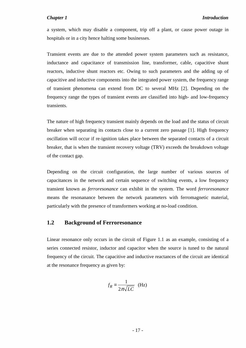
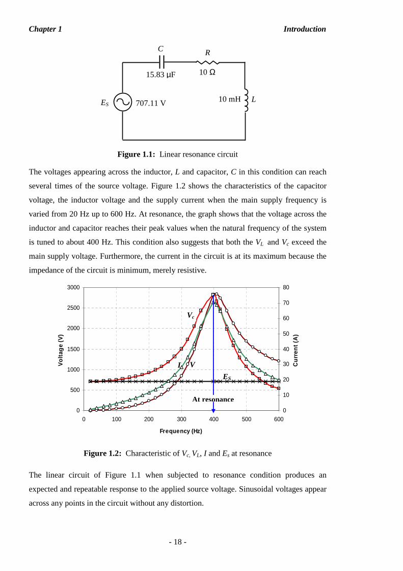
Figure 1.1: Linear resonance circuit
The voltages appearing across the inductor, L and capacitor, C in this condition can reach
several times of the source voltage. Figure 1.2 shows the characteristics of the capacitor
voltage, the inductor voltage and the supply current when the main supply frequency is
varied from 20 Hz up to 600 Hz. At resonance, the graph shows that the voltage across the
inductor and capacitor reaches their peak values when the natural frequency of the system
is tuned to about 400 Hz. This condition also suggests that both the VL and Vc exceed the
main supply voltage. Furthermore, the current in the circuit is at its maximum because the
impedance of the circuit is minimum, merely resistive.
Figure 1.2: Characteristic of Vc, VL, I and Es at resonance
The linear circuit of Figure 1.1 when subjected to resonance condition produces an
expected and repeatable response to the applied source voltage. Sinusoidal voltages appear
across any points in the circuit without any distortion.
R
L
C
ES 707.11 V
15.83 µF 10 Ω
10 mH
0
500
1000
1500
2000
2500
3000
0 100 200 300 400 500 600
Frequency (Hz)
Vol
tage
(V
)
0
10
20
30
40
50
60
70
80C
urre
nt (
A)
Vc
V
I
At resonance
ES
Vc
Chapter 1 Introduction
- 19 -
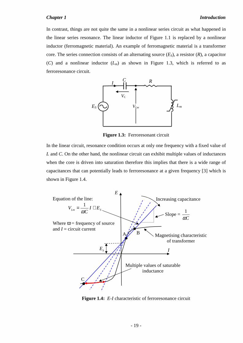
In contrast, things are not quite the same in a nonlinear series circuit as what happened in
the linear series resonance. The linear inductor of Figure 1.1 is replaced by a nonlinear
inductor (ferromagnetic material). An example of ferromagnetic material is a transformer
core. The series connection consists of an alternating source (ES), a resistor (R), a capacitor
(C) and a nonlinear inductor (Lm) as shown in Figure 1.3, which is referred to as
ferroresonance circuit.
Figure 1.3: Ferroresonant circuit
In the linear circuit, resonance condition occurs at only one frequency with a fixed value of
L and C. On the other hand, the nonlinear circuit can exhibit multiple values of inductances
when the core is driven into saturation therefore this implies that there is a wide range of
capacitances that can potentially leads to ferroresonance at a given frequency [3] which is
shown in Figure 1.4.
Figure 1.4: E-I characteristic of ferroresonance circuit
E
I
A B
C
SE
Increasing capacitance
Magnetising characteristic of transformer
Slope = 1
Cω
Multiple values of saturable inductance
Equation of the line: 1
Lm SV I ECω
= +
Where ω = frequency of source and I = circuit current
ES
R
Lm
C
VLm
VC
I
Chapter 1 Introduction
- 20 -
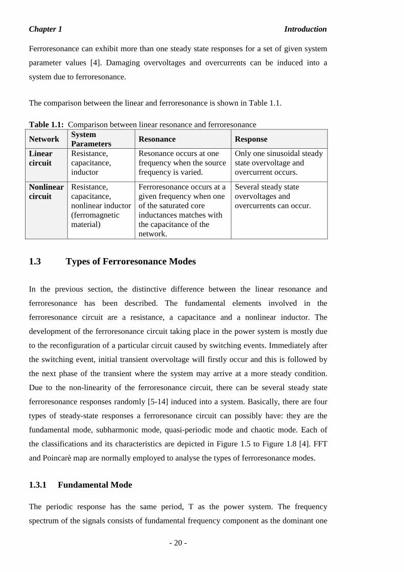
Ferroresonance can exhibit more than one steady state responses for a set of given system
parameter values [4]. Damaging overvoltages and overcurrents can be induced into a
system due to ferroresonance.
The comparison between the linear and ferroresonance is shown in Table 1.1.
Table 1.1: Comparison between linear resonance and ferroresonance
Network System Parameters
Resonance Response
Linear circuit
Resistance, capacitance, inductor
Resonance occurs at one frequency when the source frequency is varied.
Only one sinusoidal steady state overvoltage and overcurrent occurs.
Nonlinear circuit
Resistance, capacitance, nonlinear inductor (ferromagnetic material)
Ferroresonance occurs at a given frequency when one of the saturated core inductances matches with the capacitance of the network.
Several steady state overvoltages and overcurrents can occur.
1.3 Types of Ferroresonance Modes
In the previous section, the distinctive difference between the linear resonance and
ferroresonance has been described. The fundamental elements involved in the
ferroresonance circuit are a resistance, a capacitance and a nonlinear inductor. The
development of the ferroresonance circuit taking place in the power system is mostly due
to the reconfiguration of a particular circuit caused by switching events. Immediately after
the switching event, initial transient overvoltage will firstly occur and this is followed by
the next phase of the transient where the system may arrive at a more steady condition.
Due to the non-linearity of the ferroresonance circuit, there can be several steady state
ferroresonance responses randomly [5-14] induced into a system. Basically, there are four
types of steady-state responses a ferroresonance circuit can possibly have: they are the
fundamental mode, subharmonic mode, quasi-periodic mode and chaotic mode. Each of
the classifications and its characteristics are depicted in Figure 1.5 to Figure 1.8 [4]. FFT
and Poincarè map are normally employed to analyse the types of ferroresonance modes.
1.3.1 Fundamental Mode
The periodic response has the same period, T as the power system. The frequency
spectrum of the signals consists of fundamental frequency component as the dominant one
Chapter 1 Introduction
- 21 -
followed by decreasing contents of 3rd, 5th, 7th and nth odd harmonic. In addition, this type
of response can also be identified by using the stroboscopic diagram of Figure 1.5 (c)
which is also known as Poincarè plot, which can be obtained by simultaneously sampling
of voltage, v and current, i at the fundamental frequency. Detailed explanation on this plot
can be referred in the following section.
Figure 1.5: Fundamental mode
1.3.2 Subharmonic Mode
This type of ferroresonance signals has a period which is multiple of the source period, nT.
The fundamental mode of ferroresonance is normally called a Period-1 (i.e. f0/1 Hz)
ferroresonance and a ferroresonance with a sub-multiple of the power system frequency is
called a Period-n (i.e. f0/n Hz) ferroresonance. Alternatively, the frequency contents are
described having a spectrum of frequencies equal to f0/n with f0 denoting the fundamental
frequency and n is an integer. With this signal, there are n points exist in the stroboscopic
diagram which signifies predominant of fundamental frequency component with
decreasing harmonic contents at other frequencies.
Figure 1.6: Subharmonic mode
(a) Periodic signal (b) Frequency spectrum (c) Stroboscopic diagram
(a) Periodic signal (b) Frequency spectrum (c) Stroboscopic diagram
Chapter 1 Introduction
- 22 -
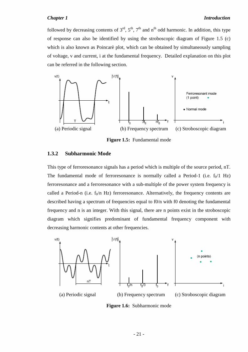
1.3.3 Quasi-periodic Mode
This kind of signal is not periodic. The frequency contents in the signal are discontinuous
in the frequency spectrum, whose frequencies are defined as: nf1+mf2 (where n and m are
integers and f1/f2 an irrational real number). This type of response displays a feature
employing a close cycle of dotted points on the stroboscopic plot. The set of points (closed
curve) in the diagram is called an attractor to which all close by orbits will asympotate as
t→ ∞, that is, in the steady state [73].
Figure 1.7: Quasi-periodic mode
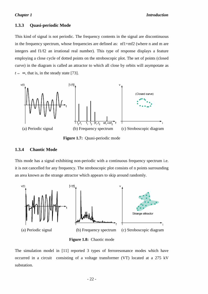
1.3.4 Chaotic Mode
This mode has a signal exhibiting non-periodic with a continuous frequency spectrum i.e.
it is not cancelled for any frequency. The stroboscopic plot consists of n points surrounding
an area known as the strange attractor which appears to skip around randomly.
Figure 1.8: Chaotic mode
The simulation model in [11] reported 3 types of ferroresonance modes which have
occurred in a circuit consisting of a voltage transformer (VT) located at a 275 kV
substation.
(a) Periodic signal (b) Frequency spectrum (c) Stroboscopic diagram
(a) Periodic signal (b) Frequency spectrum (c) Stroboscopic diagram
Chapter 1 Introduction
- 23 -
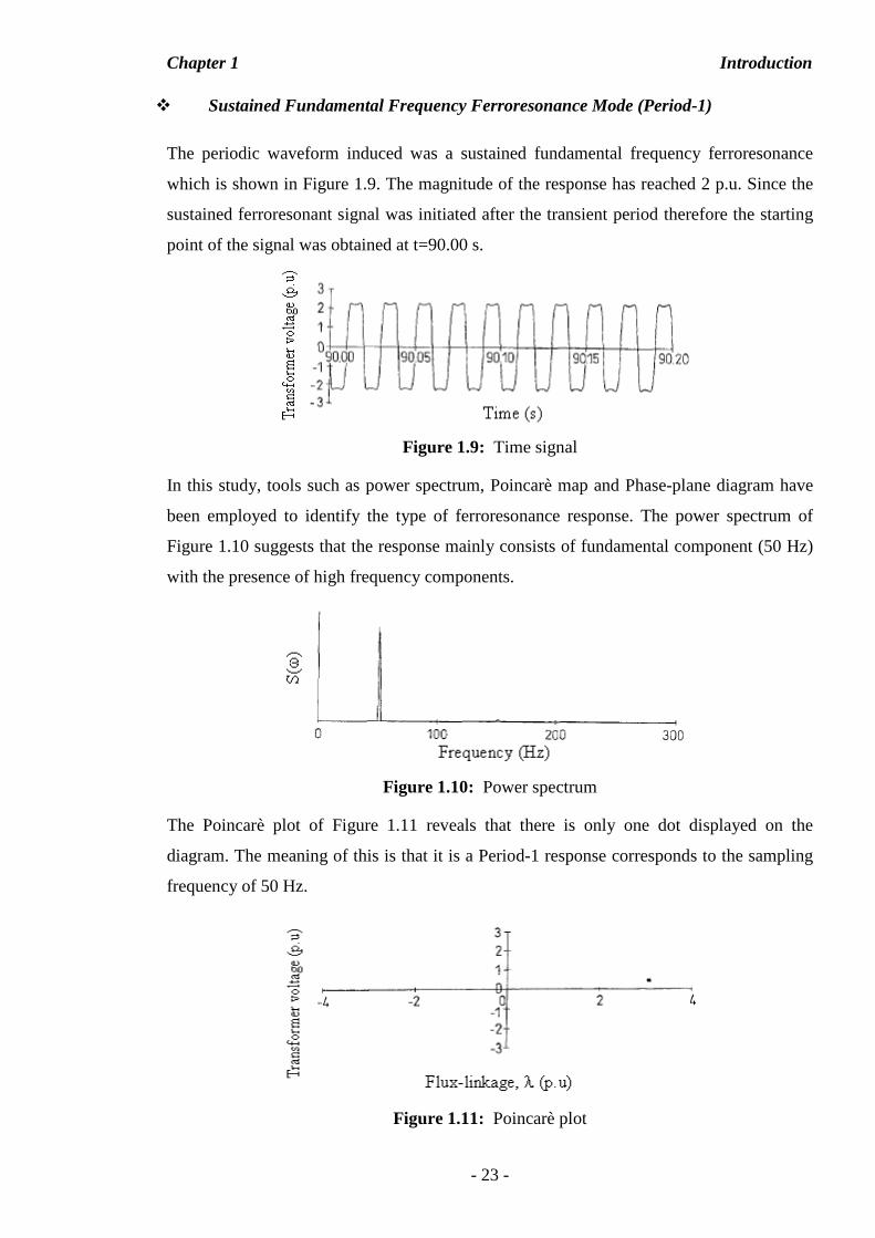
Sustained Fundamental Frequency Ferroresonance Mode (Period-1)
The periodic waveform induced was a sustained fundamental frequency ferroresonance
which is shown in Figure 1.9. The magnitude of the response has reached 2 p.u. Since the
sustained ferroresonant signal was initiated after the transient period therefore the starting
point of the signal was obtained at t=90.00 s.
Figure 1.9: Time signal
In this study, tools such as power spectrum, Poincarè map and Phase-plane diagram have
been employed to identify the type of ferroresonance response. The power spectrum of
Figure 1.10 suggests that the response mainly consists of fundamental component (50 Hz)
with the presence of high frequency components.
Figure 1.10: Power spectrum
The Poincarè plot of Figure 1.11 reveals that there is only one dot displayed on the
diagram. The meaning of this is that it is a Period-1 response corresponds to the sampling
frequency of 50 Hz.
Figure 1.11: Poincarè plot
Chapter 1 Introduction
- 24 -
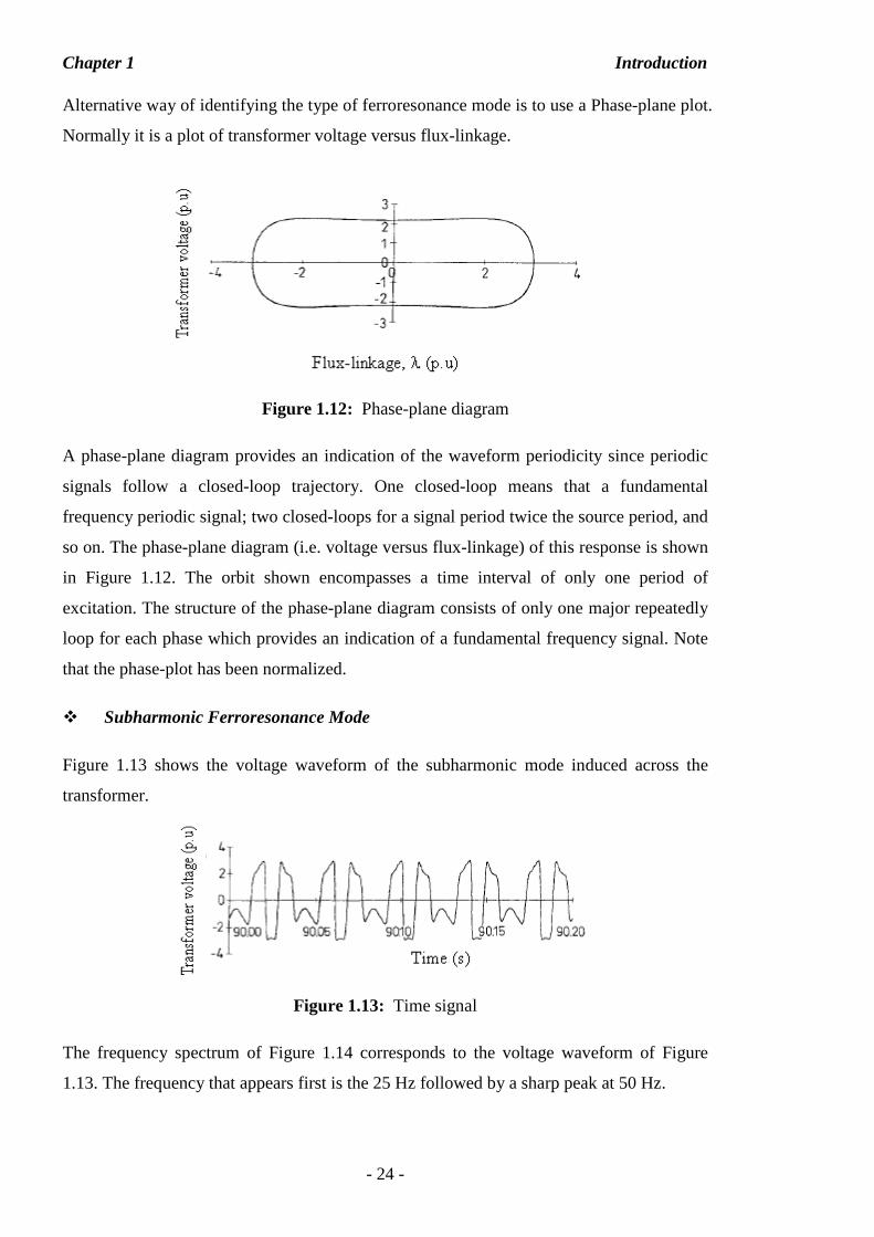
Alternative way of identifying the type of ferroresonance mode is to use a Phase-plane plot.
Normally it is a plot of transformer voltage versus flux-linkage.
Figure 1.12: Phase-plane diagram
A phase-plane diagram provides an indication of the waveform periodicity since periodic
signals follow a closed-loop trajectory. One closed-loop means that a fundamental
frequency periodic signal; two closed-loops for a signal period twice the source period, and
so on. The phase-plane diagram (i.e. voltage versus flux-linkage) of this response is shown
in Figure 1.12. The orbit shown encompasses a time interval of only one period of
excitation. The structure of the phase-plane diagram consists of only one major repeatedly
loop for each phase which provides an indication of a fundamental frequency signal. Note
that the phase-plot has been normalized.
Subharmonic Ferroresonance Mode
Figure 1.13 shows the voltage waveform of the subharmonic mode induced across the
transformer.
Figure 1.13: Time signal
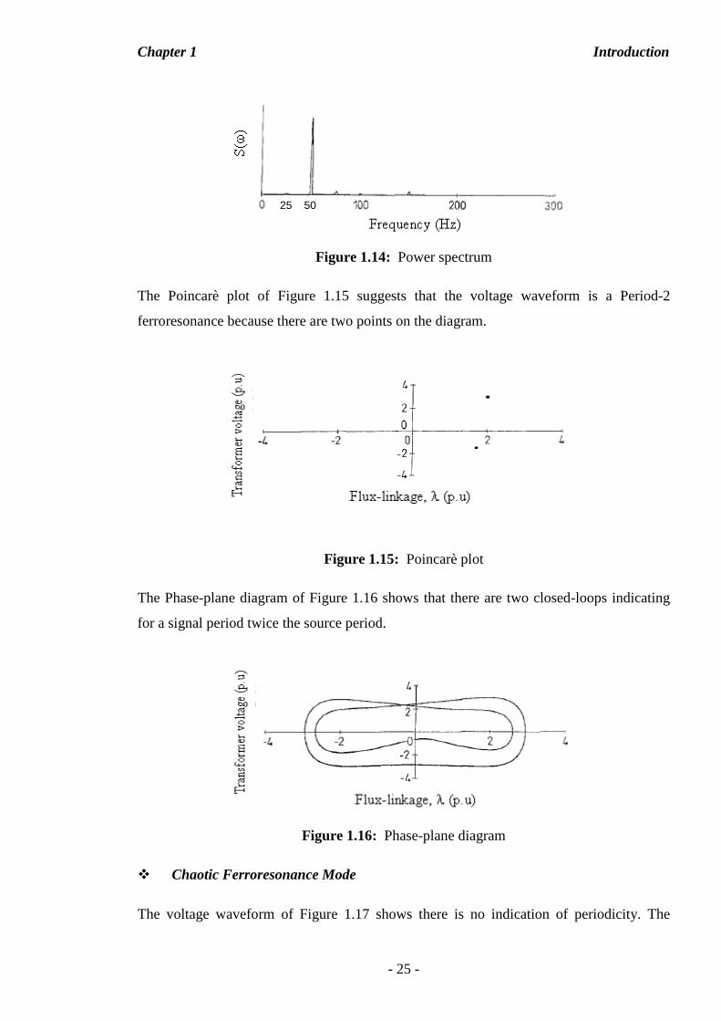
The frequency spectrum of Figure 1.14 corresponds to the voltage waveform of Figure
1.13. The frequency that appears first is the 25 Hz followed by a sharp peak at 50 Hz.
Chapter 1 Introduction
- 25 -
Figure 1.14: Power spectrum
The Poincarè plot of Figure 1.15 suggests that the voltage waveform is a Period-2
ferroresonance because there are two points on the diagram.
Figure 1.15: Poincarè plot
The Phase-plane diagram of Figure 1.16 shows that there are two closed-loops indicating
for a signal period twice the source period.
Figure 1.16: Phase-plane diagram
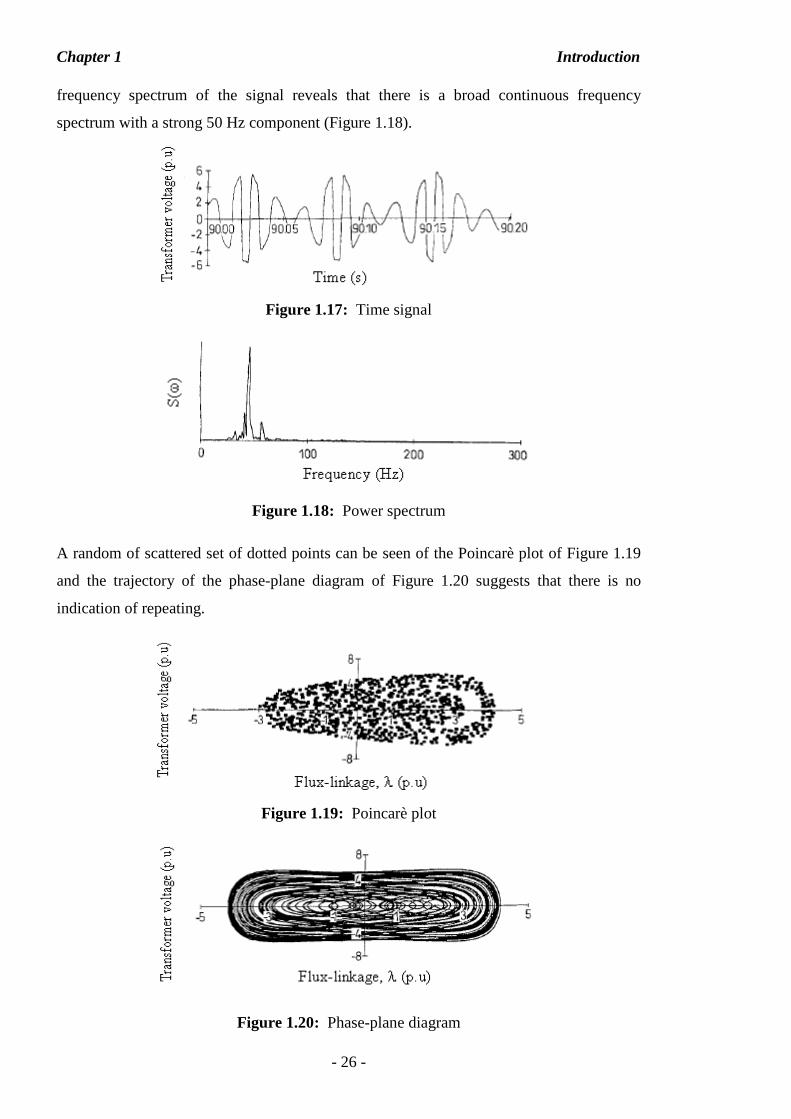
Chaotic Ferroresonance Mode
The voltage waveform of Figure 1.17 shows there is no indication of periodicity. The
50 25
Chapter 1 Introduction
- 26 -
frequency spectrum of the signal reveals that there is a broad continuous frequency
spectrum with a strong 50 Hz component (Figure 1.18).
Figure 1.17: Time signal
Figure 1.18: Power spectrum
A random of scattered set of dotted points can be seen of the Poincarè plot of Figure 1.19
and the trajectory of the phase-plane diagram of Figure 1.20 suggests that there is no
indication of repeating.
Figure 1.19: Poincarè plot
Figure 1.20: Phase-plane diagram
Chapter 1 Introduction
- 27 -
1.4 Effect of Ferroresonance on Power Systems
In the preceding section, the characteristics and features of each of the four distinctive
ferroresonance modes have been highlighted. The impacts due to ferroresonance can cause
undesirable effects on power system components. The implications of such phenomena
experienced in [7, 14-16] have been reported. They are summarised as follows:
• [15] described that a 420-kV peak and distorted sustained fundamental mode
ferroresonance waveform has been induced in C-phase 1000 MVA, 525/241.5-kV
wye-connected bank of autotransformers. The consequences following the event
were as follows: Nine minutes later, the gas accumulation alarm relay operated on
the C-phase transformer. Arcing of C-phase switch was much more severe than
that of the other two phases. No sign of damage although a smell of burnt
insulation was reported. However, the gas analysis reported a significant amount
of hydrogen, carbon dioxide and monoxide.
• Ferroresonance experienced in [14] was due to the switching events that have
been carried out during the commissioning of a new 400-kV substation. It was
reported that two voltage transformers (VT) terminating into the system had been
driven into a sustained fundamental frequency ferroresonance of 2 p.u. The
adverse impact upon the initiation of this phenomenon was that a very loud
humming noise generated from the affected voltage transformer, heard by the
local operator.
• In 1995, [16] reported that one of the buses in the station was disconnected from
service for the purpose of commissioning the replaced circuit breaker and current
transformers. At the same time, work on maintenance and trip testing were also
carried out. After the switching operations, the potential transformers which were
connected at the de-energised bus were energised by the adjacent live busbar, via
the circuit breakers’ grading capacitors. Following the switching events, a
sustained fundamental frequency ferroresonance has been induced into the system.
As a result, the response has caused an explosion to the potential transformer. The
catastrophically failure was due to the excessive current in the primary winding of
the affected potential transformer.
Chapter 1 Introduction
- 28 -
• [7] reported that the Station Service Transformer (SST) ferroresonance has been
occurred at the 12-kV substation. The incident was due to the switching
operations by firstly opening the circuit breaker and then the disconnector switch
located at the riser pole surge arrester. The first ferroresonance test without
arrestor installation has induced both the 3rd subharmonic and chaotic modes. As a
result, the affected transformer creating loud noises like sound of crack and race
engine. While for the second test, with the arrester, a sustained fundamental mode
has been generated and thus has caused the explosion of riser pole arrester. The
physical impact of the explosion has caused the ground lead of the disconnector
explodes and the ruptures of the polymer housing.
It has been addressed from the above that the trigger mechanism of ferroresonance is
switching events that reconfigure a circuit into ferroresonance circuit. In addition, the
literatures presented in [3, 17, 18] documented that the existence of the phenomena can
also result in any of the following symptom(s):
- Inappropriate time operation of protective devices and interference of
control operation [3, 4, 18].
- Electrical equipment damage due to thermal effect or insulation
breakdown and internal transformer heating triggering of the Bucholtz
relay [3, 4, 18].
- Arcing across open phase switches or over surge arresters, particularly
the use of the gapless ZnO [14].
- Premature ageing of equipment insulation structures [17].
Owing to the above consequences and symptoms, mitigation measures of ferroresonance
are therefore necessary in order for the system to operate in a healthy environment.
1.5 Mitigation of Ferroresonance
The initiation of ferroresonance phenomena can cause distorted overvoltages and
overcurrents to be induced into a system. The outcomes of this event have been highlighted
in section 1.4 which are considered to be catastrophic when it occurs. There are generally
two main ways of preventing the occurrence of ferroresonance [3, 4, 17].
Chapter 1 Introduction
- 29 -
Avoid any switching operations that will reconfigure a circuit into a sudden
inclusion of capacitance connected in series with transformer with no or light load
condition [17].
Provide damping of ferroresonance by introducing losses (i.e. load resistance) into
the affected transformer. In other words, there is not sufficient energy supplied by
the source to sustain the response [3, 4, 17].
1.6 Motivation
A survey paying attention onto the modeling of power system components for
ferroresonance simulation study has been highlighted in the literature review in Chapter 2.
It is shown that the main objective of developing the simulation models focused on
validation of the models using the field test ferroresonance waveforms, then the use of the
simulation tools to analyse the types of ferroresonant modes and finally performing the
mitigation studies of ferroresonance. One of the main problems that ferroresonance studies
employing digital simulation programs face is the lack of definitive criterion on how each
of the power system components should be modeled. There is lacking of detailed
guidelines on how the power system components such as the voltage source, transformer,
transmission line, cable and circuit breaker should be modeled for ferroresonance studies.
In addition, step-by-step systematic approaches of selecting an appropriate simulation
model are still not explained in the literatures. Therefore, the motivation devoted in this
thesis is directed towards achieving the following objectives:
To provide a better understanding about the technical requirements on each of the
power system components necessary for the development of simulation models for
ferroresonance study.
To provide a set of modeling guidelines required for choosing any of the available
models.
To identify the types of models suitable for the simulation studies required in this
thesis.
Chapter 1 Introduction
- 30 -
To achieve the above objectives, a simulation model has been built on a 400/275 kV sub-
transmission system undergone ferroresonance tests. Verification of the simulation results
with the field test recordings have been performed, particularly the 50 Hz fundamental and
16.67 Hz subharmonic mode ferroresonance.
Based on the reasonable matching between the simulation and the field test recording
waveforms, the modeling techniques which have been developed are then applied for the
ferroresonance study of 400/275 kV sub-transmission system with the aim of assessing
whether there is any likelihood of 50 Hz sustained fundamental frequency mode which can
be initiated in the system, and also investigating an effective switch-in shunt reactor
connected at the 13 kV tertiary winding for quenching purpose.
1.7 Methodology
The undesirable effects of ferroresonance phenomena subjected to power system
components have been highlighted in section 1.4. Building a realistic model that would
satisfactorily model such a transient event, employed either one of the following methods
(1) analytical approach (2) analog simulation approach (3) real field test approach (4)
laboratory measurement approach and (5) digital computer program approach.
Power system transient represented by analytical approach is difficult because of lengthy
mathematical equations involved in arriving at the solutions required. Using analog
simulators such as Transient Network Analyser (TNA) [19], the miniature approach of
characterising power system model is rather expensive and requires floor areas to
accommodate the equipment. Real network testing performed in the field is considered to
be impractical at the design stage of a power system network. In view of those, a computer
simulation program is therefore preferred as compared to the previous approaches. In this
project, a graphical user interface (GUI) with a mouse-driven approach software called
ATPDraw is employed. In this program, the users can develop the simulation models of
digital representation of the power circuit under study, by simply choosing the build-in
predefined components.
To develop a complete simulation model in ATPDraw, a block diagram as shown in
Figure 1.21 is firstly drawn up outlining the approach which should be followed for
simulation studies.
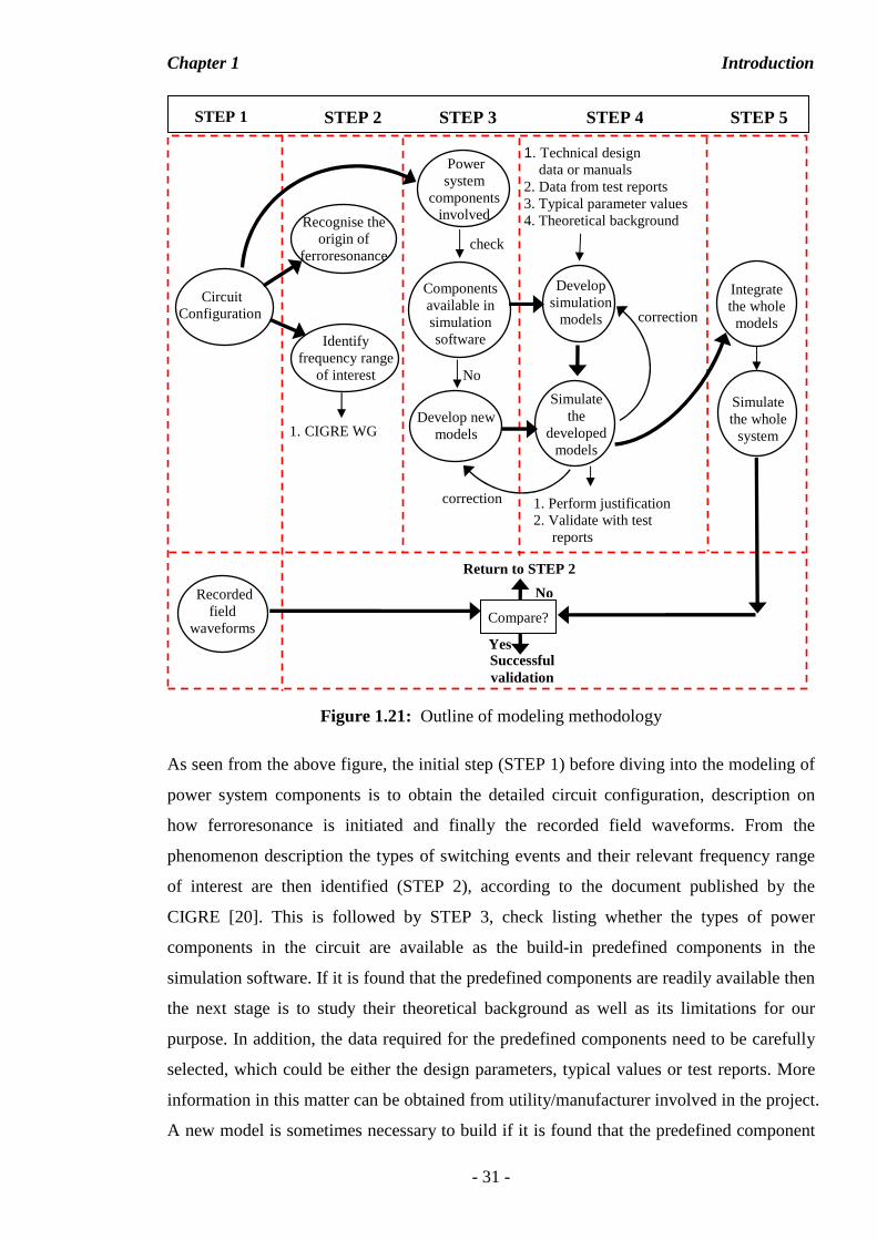
Chapter 1 Introduction
- 31 -
Figure 1.21: Outline of modeling methodology
As seen from the above figure, the initial step (STEP 1) before diving into the modeling of
power system components is to obtain the detailed circuit configuration, description on
how ferroresonance is initiated and finally the recorded field waveforms. From the
phenomenon description the types of switching events and their relevant frequency range
of interest are then identified (STEP 2), according to the document published by the
CIGRE [20]. This is followed by STEP 3, check listing whether the types of power
components in the circuit are available as the build-in predefined components in the
simulation software. If it is found that the predefined components are readily available then
the next stage is to study their theoretical background as well as its limitations for our
purpose. In addition, the data required for the predefined components need to be carefully
selected, which could be either the design parameters, typical values or test reports. More
information in this matter can be obtained from utility/manufacturer involved in the project.
A new model is sometimes necessary to build if it is found that the predefined component
Develop simulation
models
1. Technical design data or manuals 2. Data from test reports 3. Typical parameter values 4. Theoretical background
Simulate the
developed models
1. Perform justification 2. Validate with test reports
Circuit Configuration
Recorded field
waveforms
Recognise the origin of
ferroresonance
Identify frequency range
of interest
Components available in simulation software
Develop new models
Power system
components involved
check
No
correction
Integrate the whole models
Simulate the whole
system
Compare?
STEP 1 STEP 2 STEP 3 STEP 4 STEP 5
Successful validation
correction
1. CIGRE WG
Return to STEP 2
No
Yes
Chapter 1 Introduction
- 32 -
cannot serve the modeling requirements. Once the new or the predefined components have
been developed, the next phase is to conduct validation and simulation studies. Once each
of the developed simulation model has been tested or checked accordingly, then they are
integrated into the actual circuit configuration. The simulation results are then compared
with the actual field recorded waveform for validation. The process is then repeated if it is
found out that the comparisons do not match what are expected.
Once the developed simulation model has been verified, the next stage of the simulation
study can be scenario studies or sensitivity studies, aimed for in advance forecasting the
consequences of switching operations of a power system network and planning for
protection schemes. As an example, designing and evaluations of damping and quenching
devices and to determine the thermal withstand capability of the devices can be parts of the
study.
1.8 Thesis structure
There are seven chapters in this thesis. Overall they can be divided into four sections.
Chapter 1 and 2 consist of the background; the objectives, the motivation, the methodology
and literature review. Chapter 3 mainly concerns with exploring and understanding the
behaviour of ferroresonance phenomenon and this leads into chapter 4 looking into
modeling aspects of circuit breakers, transformers and transmission lines. The final stage
of the project i.e. the development of two simulation models for two practical case
scenarios, is covered in Chapter 5 and Chapter 6, followed by highlighting the contribution
of the work and the work for future research.
Chapter 1: Introduction
In the first chapter, an overview of power system network and the introduction of the
aspects of ferroresonance in terms of its occurrence, configuration, responses, impact and
mitigation are introduced. In addition, the motivation together with the objective and the
methodology of the projected are defined in this chapter.
Chapter 1 Introduction
- 33 -
Chapter 2: Literature Review
In this chapter, five different types of technology for time domain modeling ferroresonance,
particularly the way that the components are taken into consideration are reviewed. Their
advantages and disadvantages are emphased and compared with computer simulation
program approach. The main issues encountered in modeling the real case system are
highlighted here.
Chapter 3: Single-Phase Ferroresonance – A Case Study
The main aims of this chapter are twofold by considering an existing real case scenario
including a single-phase equivalent transformer model connected to the circuit breaker
including its grading capacitor and the influence of shunt capacitor of busbar. The first aim
is to look into the influence of the core-loss and the degrees of core saturations. The
second one is to investigate on how the initiation of fundamental and subharmonic mode
ferroresonance can occur when being affected by both the grading capacitor and the shunt
capacitor.
Chapter 4: System Component Models for Ferroresonance
This chapter concentrates on the modeling aspects of the power system component
available in ATPDraw suitable for the study of ferroresonance, particularly looking into
the circuit breaker, the transformers and the transmission lines. Each predefined model in
ATPDraw is reviewed to determine the suitability for ferroresonance study.
Chapter 5: Modeling of 400 kV Thorpe-Marsh/Brinsworth System
There are two main objectives covered in this chapter; firstly the validation of the
developed predefined models and secondly identifying the key parameter responsible for
the occurrence of ferroresonance. For the first objective, finding out the suitability of the
predefined models is carried out by modeling a real test case on the Thorpe-
Marsh/Brinsworth system. The only way to find out the correctness of the modeled
component is to compare the simulation results with the real field test recording results, in
terms of 3-phase voltages and currents for both the Period-1 and Period-3 ferroresonance.
An attempt in improving the deviation from the real measurement results is also conducted.
Chapter 1 Introduction
- 34 -
The second objective is to identify which parameter in the transmission system is the key
parameter to cause ferroresonance to occur. Three components are believed to dominant
the influence of ferroresonance; they are the transformer’s coupling capacitor, the cable
capacitors and the transmission line coupling capacitors. The transmission line is modeled
as a lumped element in PI representation. The way to find out their influence is by
simulating the system stage by stage without firstly including the transformer’s coupling
capacitors and then secondly simulating the system without the presence of cable
capacitance, and finally looking into the individual capacitors of the line.
Chapter 6: Modeling of 400 kV Iron-Action/Melksham System
Following the modeling experiences which are gained from Chapter 5, modeling of
another real case system “Iron-Acton/Melksham system” is carried out in this chapter. The
system is believed to have potential risk of initiating Period-1 ferroresonance because of
the complex arrangement of the mesh-corner substation. The inquiry from National Grid is
to evaluate the system whether there is any likelihood of occurrence Period-1
ferroresonance. If it does, a mitigation measure by employing a shunt reactor connected to
the 13 kV winding is suggested to switch-in. The power rating of shunt reactor is chosen
according to a series of evaluations so that the ferroresonance is effectively suppressed
without any failure. In addition, sensitivity study on transmission line lengths is also
carried out to determine the probability function of occurrence of various ferroresonance
modes.
Chapter 7: Conclusion and Future work
In this last chapter, the conclusion for each chapter is drawn along with the papers
published as a result of this work. The contribution towards the users about this work and
finally the room for future work is highlighted.
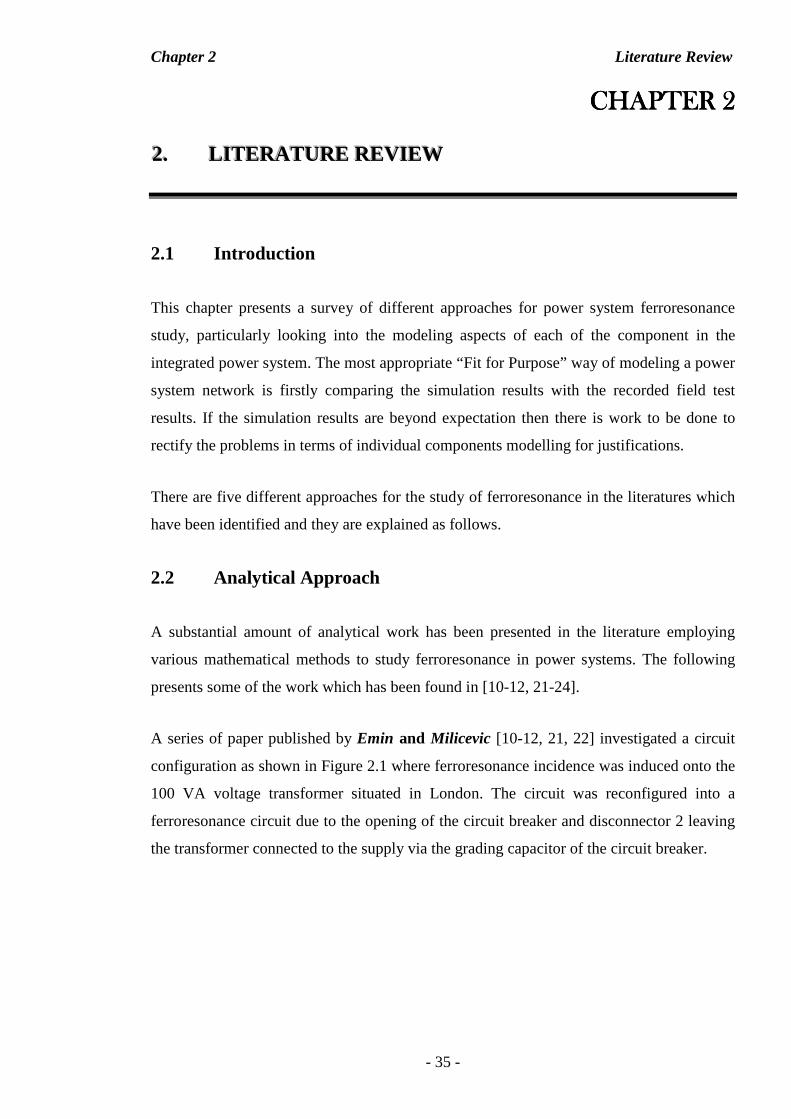
Chapter 2 Literature Review
- 35 -
CHAPTER 2CHAPTER 2CHAPTER 2CHAPTER 2
222... LLL III TTTEEERRRAAATTTUUURRREEE RRREEEVVVIII EEEWWW
2.1 Introduction
This chapter presents a survey of different approaches for power system ferroresonance
study, particularly looking into the modeling aspects of each of the component in the
integrated power system. The most appropriate “Fit for Purpose” way of modeling a power
system network is firstly comparing the simulation results with the recorded field test
results. If the simulation results are beyond expectation then there is work to be done to
rectify the problems in terms of individual components modelling for justifications.
There are five different approaches for the study of ferroresonance in the literatures which
have been identified and they are explained as follows.
2.2 Analytical Approach
A substantial amount of analytical work has been presented in the literature employing
various mathematical methods to study ferroresonance in power systems. The following
presents some of the work which has been found in [10-12, 21-24].
A series of paper published by Emin and Milicevic [10-12, 21, 22] investigated a circuit
configuration as shown in Figure 2.1 where ferroresonance incidence was induced onto the
100 VA voltage transformer situated in London. The circuit was reconfigured into a
ferroresonance circuit due to the opening of the circuit breaker and disconnector 2 leaving
the transformer connected to the supply via the grading capacitor of the circuit breaker.
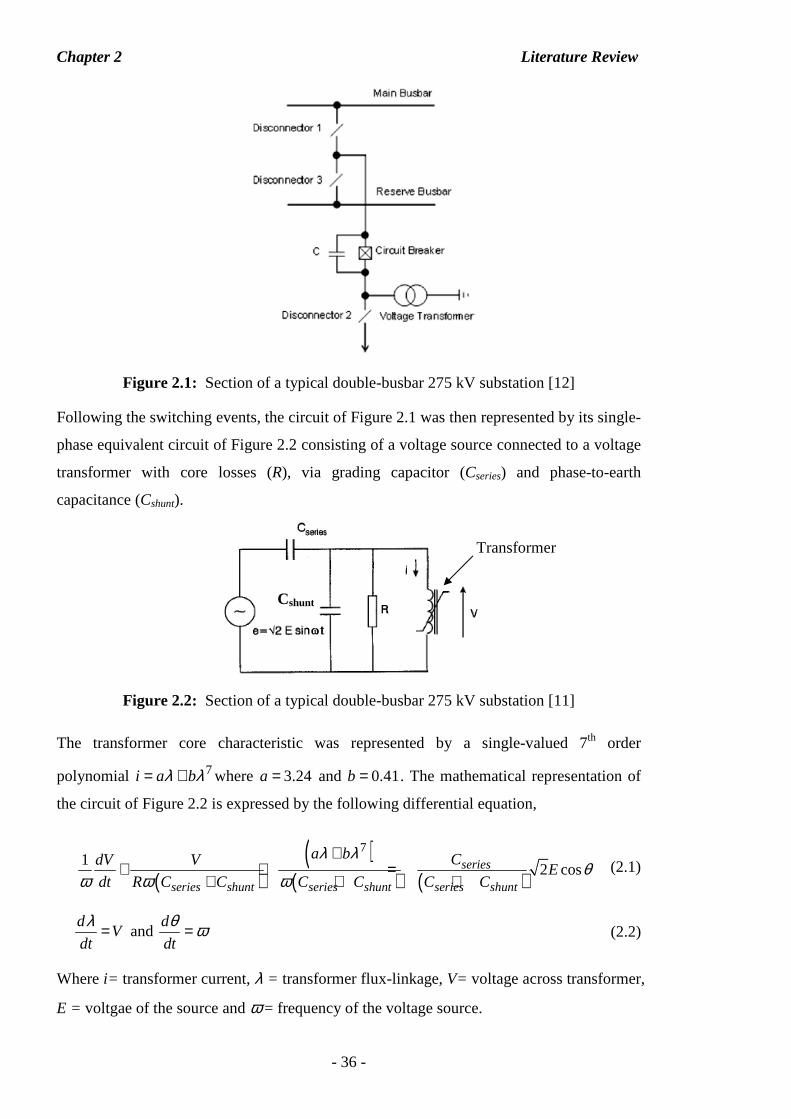
Chapter 2 Literature Review
- 36 -
Figure 2.1: Section of a typical double-busbar 275 kV substation [12]
Following the switching events, the circuit of Figure 2.1 was then represented by its single-
phase equivalent circuit of Figure 2.2 consisting of a voltage source connected to a voltage
transformer with core losses (R), via grading capacitor (Cseries) and phase-to-earth
capacitance (Cshunt).
Figure 2.2: Section of a typical double-busbar 275 kV substation [11]
The transformer core characteristic was represented by a single-valued 7th order
polynomial 7i a bλ λ= + where 3.24a = and 0.41b = . The mathematical representation of
the circuit of Figure 2.2 is expressed by the following differential equation,
( )
( )( ) ( )
71
2 cosseries
series shunt series shunt series shunt
a b CdV VE
dt R C C C C C C
λ λθ
ω ω ω
++ + =
+ + + (2.1)
d
Vdt
λ = and d
dt
θ ω= (2.2)
Where i= transformer current, λ = transformer flux-linkage, V= voltage across transformer,
E = voltgae of the source and ω = frequency of the voltage source.
Cshunt
Transformer
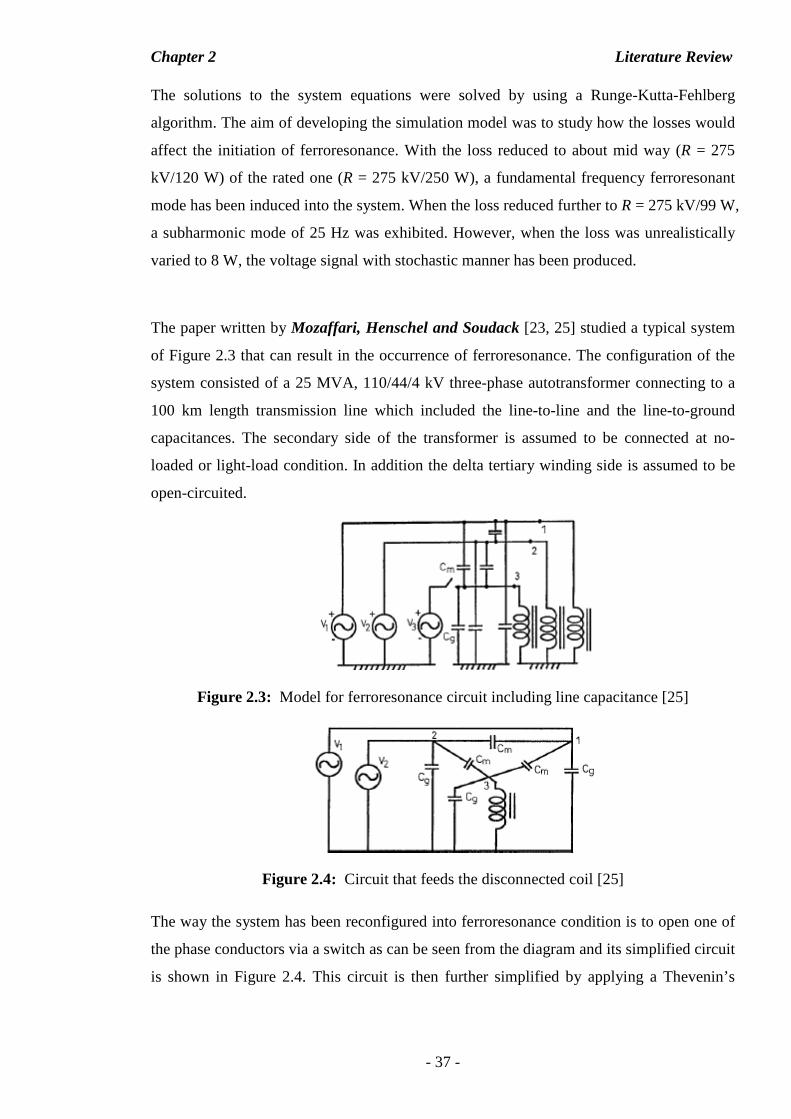
Chapter 2 Literature Review
- 37 -
The solutions to the system equations were solved by using a Runge-Kutta-Fehlberg
algorithm. The aim of developing the simulation model was to study how the losses would
affect the initiation of ferroresonance. With the loss reduced to about mid way (R = 275
kV/120 W) of the rated one (R = 275 kV/250 W), a fundamental frequency ferroresonant
mode has been induced into the system. When the loss reduced further to R = 275 kV/99 W,
a subharmonic mode of 25 Hz was exhibited. However, when the loss was unrealistically
varied to 8 W, the voltage signal with stochastic manner has been produced.
The paper written by Mozaffari, Henschel and Soudack [23, 25] studied a typical system
of Figure 2.3 that can result in the occurrence of ferroresonance. The configuration of the
system consisted of a 25 MVA, 110/44/4 kV three-phase autotransformer connecting to a
100 km length transmission line which included the line-to-line and the line-to-ground
capacitances. The secondary side of the transformer is assumed to be connected at no-
loaded or light-load condition. In addition the delta tertiary winding side is assumed to be
open-circuited.
Figure 2.3: Model for ferroresonance circuit including line capacitance [25]
Figure 2.4: Circuit that feeds the disconnected coil [25]
The way the system has been reconfigured into ferroresonance condition is to open one of
the phase conductors via a switch as can be seen from the diagram and its simplified circuit
is shown in Figure 2.4. This circuit is then further simplified by applying a Thevenin’s
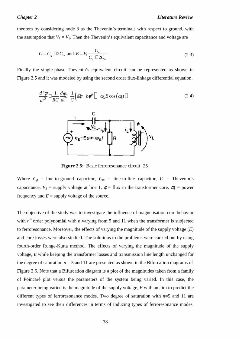
Chapter 2 Literature Review
- 38 -
theorem by considering node 3 as the Thevenin’s terminals with respect to ground, with
the assumption that V1 = V2. Then the Thevenin’s equivalent capacitance and voltage are
2g mC C C= + and 1 2m
g m
CE V
C C=
+ (2.3)
Finally the single-phase Thevenin’s equivalent circuit can be represented as shown in
Figure 2.5 and it was modeled by using the second order flux-linkage differential equation.
( ) ( )2
21 1
cosns s
d da b E t
RC dt Cdt
φ φ φ φ ω ω+ + + = (2.4)
Figure 2.5: Basic ferroresonance circuit [25]
Where Cg = line-to-ground capacitor, Cm = line-to-line capacitor, C = Thevenin’s
capacitance, V1 = supply voltage at line 1, φ = flux in the transformer core, ωs = power
frequency and E = supply voltage of the source.
The objective of the study was to investigate the influence of magnetisation core behavior
with nth order polynomial with n varying from 5 and 11 when the transformer is subjected
to ferroresonance. Moreover, the effects of varying the magnitude of the supply voltage (E)
and core losses were also studied. The solutions to the problems were carried out by using
fourth-order Runge-Kutta method. The effects of varying the magnitude of the supply
voltage, E while keeping the transformer losses and transmission line length unchanged for
the degree of saturation n = 5 and 11 are presented as shown in the Bifurcation diagrams of
Figure 2.6. Note that a Bifurcation diagram is a plot of the magnitudes taken from a family
of Poincarè plot versus the parameters of the system being varied. In this case, the
parameter being varied is the magnitude of the supply voltage, E with an aim to predict the
different types of ferroresonance modes. Two degree of saturation with n=5 and 11 are
investigated to see their differences in terms of inducing types of ferroresonance modes.
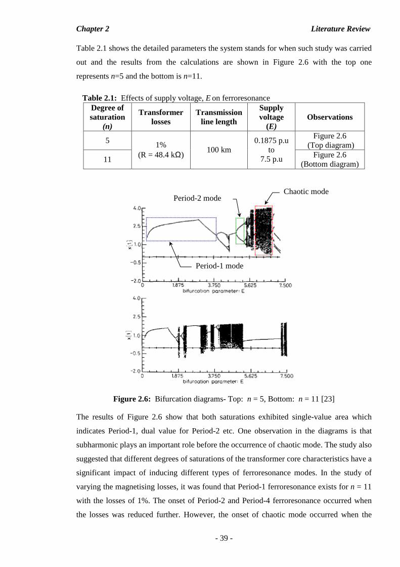
Chapter 2 Literature Review
- 39 -
Table 2.1 shows the detailed parameters the system stands for when such study was carried
out and the results from the calculations are shown in Figure 2.6 with the top one
represents n=5 and the bottom is n=11.
Table 2.1: Effects of supply voltage, E on ferroresonance Degree of saturation
(n)
Transformer losses
Transmission line length
Supply voltage
(E) Observations
5 Figure 2.6
(Top diagram)
11
1% (R = 48.4 kΩ)
100 km 0.1875 p.u
to 7.5 p.u Figure 2.6
(Bottom diagram)
Figure 2.6: Bifurcation diagrams- Top: n = 5, Bottom: n = 11 [23]
The results of Figure 2.6 show that both saturations exhibited single-value area which
indicates Period-1, dual value for Period-2 etc. One observation in the diagrams is that
subharmonic plays an important role before the occurrence of chaotic mode. The study also
suggested that different degrees of saturations of the transformer core characteristics have a
significant impact of inducing different types of ferroresonance modes. In the study of
varying the magnetising losses, it was found that Period-1 ferroresonance exists for n = 11
with the losses of 1%. The onset of Period-2 and Period-4 ferroresonance occurred when
the losses was reduced further. However, the onset of chaotic mode occurred when the
Period-1 mode
Period-2 mode Chaotic mode
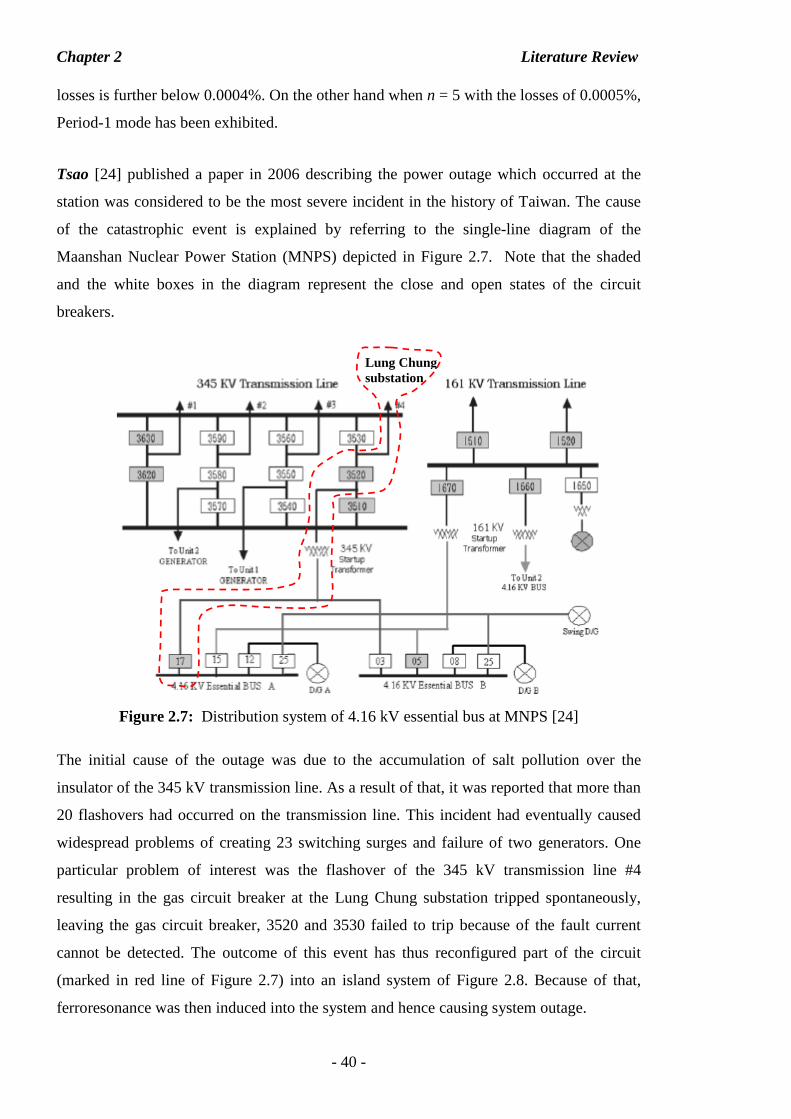
Chapter 2 Literature Review
- 40 -
losses is further below 0.0004%. On the other hand when n = 5 with the losses of 0.0005%,
Period-1 mode has been exhibited.
Tsao [24] published a paper in 2006 describing the power outage which occurred at the
station was considered to be the most severe incident in the history of Taiwan. The cause
of the catastrophic event is explained by referring to the single-line diagram of the
Maanshan Nuclear Power Station (MNPS) depicted in Figure 2.7. Note that the shaded
and the white boxes in the diagram represent the close and open states of the circuit
breakers.
Figure 2.7: Distribution system of 4.16 kV essential bus at MNPS [24]
The initial cause of the outage was due to the accumulation of salt pollution over the
insulator of the 345 kV transmission line. As a result of that, it was reported that more than
20 flashovers had occurred on the transmission line. This incident had eventually caused
widespread problems of creating 23 switching surges and failure of two generators. One
particular problem of interest was the flashover of the 345 kV transmission line #4
resulting in the gas circuit breaker at the Lung Chung substation tripped spontaneously,
leaving the gas circuit breaker, 3520 and 3530 failed to trip because of the fault current
cannot be detected. The outcome of this event has thus reconfigured part of the circuit
(marked in red line of Figure 2.7) into an island system of Figure 2.8. Because of that,
ferroresonance was then induced into the system and hence causing system outage.
Lung Chung substation
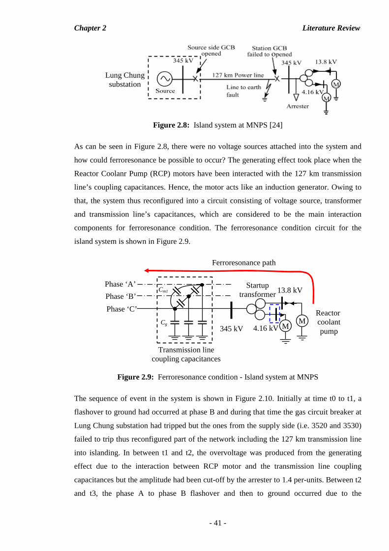
Chapter 2 Literature Review
- 41 -
Figure 2.8: Island system at MNPS [24]
As can be seen in Figure 2.8, there were no voltage sources attached into the system and
how could ferroresonance be possible to occur? The generating effect took place when the
Reactor Coolanr Pump (RCP) motors have been interacted with the 127 km transmission
line’s coupling capacitances. Hence, the motor acts like an induction generator. Owing to
that, the system thus reconfigured into a circuit consisting of voltage source, transformer
and transmission line’s capacitances, which are considered to be the main interaction
components for ferroresonance condition. The ferroresonance condition circuit for the
island system is shown in Figure 2.9.
Figure 2.9: Ferroresonance condition - Island system at MNPS
The sequence of event in the system is shown in Figure 2.10. Initially at time t0 to t1, a
flashover to ground had occurred at phase B and during that time the gas circuit breaker at
Lung Chung substation had tripped but the ones from the supply side (i.e. 3520 and 3530)
failed to trip thus reconfigured part of the network including the 127 km transmission line
into islanding. In between t1 and t2, the overvoltage was produced from the generating
effect due to the interaction between RCP motor and the transmission line coupling
capacitances but the amplitude had been cut-off by the arrester to 1.4 per-units. Between t2
and t3, the phase A to phase B flashover and then to ground occurred due to the
Lung Chung substation
M M
Cm1
Cg
Startup transformer
345 kV 4.16 kV
13.8 kV
Reactor coolant pump
Transmission line coupling capacitances
Phase ‘A’
Phase ‘B’
Phase ‘C’
Ferroresonance path
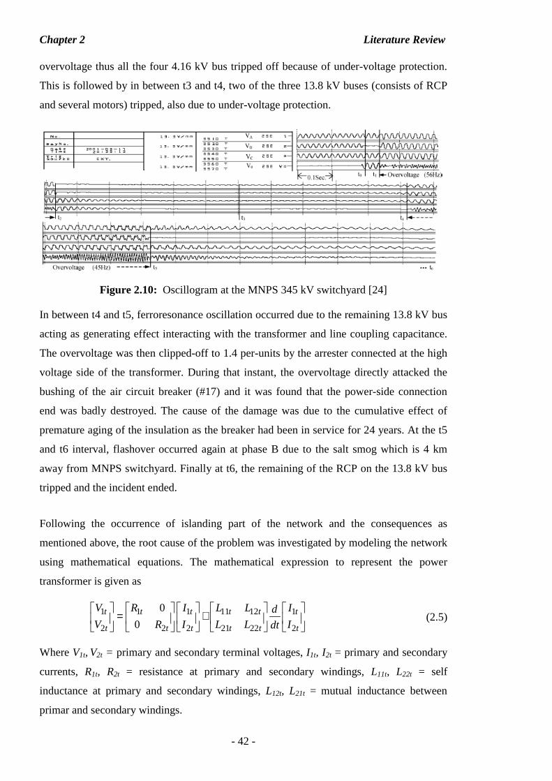
Chapter 2 Literature Review
- 42 -
overvoltage thus all the four 4.16 kV bus tripped off because of under-voltage protection.
This is followed by in between t3 and t4, two of the three 13.8 kV buses (consists of RCP
and several motors) tripped, also due to under-voltage protection.
Figure 2.10: Oscillogram at the MNPS 345 kV switchyard [24]
In between t4 and t5, ferroresonance oscillation occurred due to the remaining 13.8 kV bus
acting as generating effect interacting with the transformer and line coupling capacitance.
The overvoltage was then clipped-off to 1.4 per-units by the arrester connected at the high
voltage side of the transformer. During that instant, the overvoltage directly attacked the
bushing of the air circuit breaker (#17) and it was found that the power-side connection
end was badly destroyed. The cause of the damage was due to the cumulative effect of
premature aging of the insulation as the breaker had been in service for 24 years. At the t5
and t6 interval, flashover occurred again at phase B due to the salt smog which is 4 km
away from MNPS switchyard. Finally at t6, the remaining of the RCP on the 13.8 kV bus
tripped and the incident ended.
Following the occurrence of islanding part of the network and the consequences as
mentioned above, the root cause of the problem was investigated by modeling the network
using mathematical equations. The mathematical expression to represent the power
transformer is given as
1 1 1 11 12 1
2 2 2 21 22 2
0
0t t t t t t
t t t t t t
V R I L L Id
V R I L L Idt
= +
(2.5)
Where V1t, V2t = primary and secondary terminal voltages, I1t, I2t = primary and secondary
currents, R1t, R2t = resistance at primary and secondary windings, L11t, L22t = self
inductance at primary and secondary windings, L12t, L21t = mutual inductance between
primar and secondary windings.
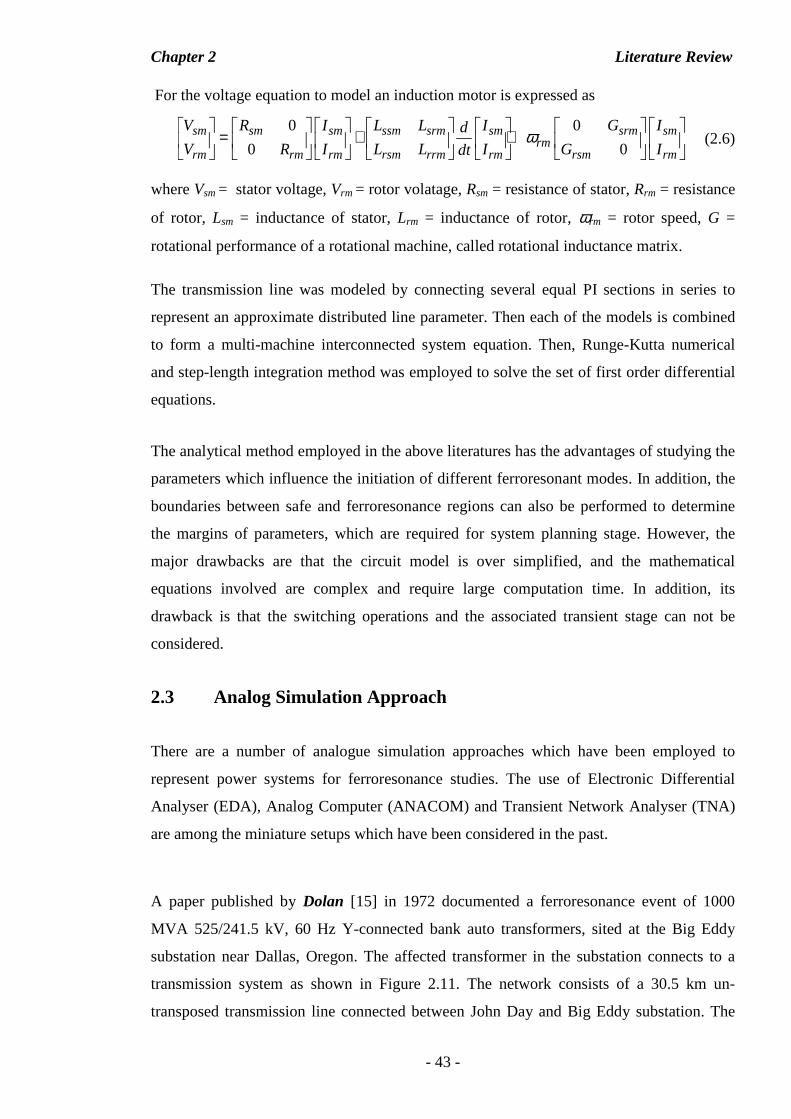
Chapter 2 Literature Review
- 43 -
For the voltage equation to model an induction motor is expressed as
0 0
0 0sm sm sm ssm srm sm srm sm
rmrm rm rm rsm rrm rm rsm rm
V R I L L I G Id
V R I L L I G Idtω
= + +
(2.6)
where Vsm = stator voltage, Vrm = rotor volatage, Rsm = resistance of stator, Rrm = resistance
of rotor, Lsm = inductance of stator, Lrm = inductance of rotor, ωrm = rotor speed, G =
rotational performance of a rotational machine, called rotational inductance matrix.
The transmission line was modeled by connecting several equal PI sections in series to
represent an approximate distributed line parameter. Then each of the models is combined
to form a multi-machine interconnected system equation. Then, Runge-Kutta numerical
and step-length integration method was employed to solve the set of first order differential
equations.
The analytical method employed in the above literatures has the advantages of studying the
parameters which influence the initiation of different ferroresonant modes. In addition, the
boundaries between safe and ferroresonance regions can also be performed to determine
the margins of parameters, which are required for system planning stage. However, the
major drawbacks are that the circuit model is over simplified, and the mathematical
equations involved are complex and require large computation time. In addition, its
drawback is that the switching operations and the associated transient stage can not be
considered.
2.3 Analog Simulation Approach
There are a number of analogue simulation approaches which have been employed to
represent power systems for ferroresonance studies. The use of Electronic Differential
Analyser (EDA), Analog Computer (ANACOM) and Transient Network Analyser (TNA)
are among the miniature setups which have been considered in the past.
A paper published by Dolan [15] in 1972 documented a ferroresonance event of 1000
MVA 525/241.5 kV, 60 Hz Y-connected bank auto transformers, sited at the Big Eddy
substation near Dallas, Oregon. The affected transformer in the substation connects to a
transmission system as shown in Figure 2.11. The network consists of a 30.5 km un-
transposed transmission line connected between John Day and Big Eddy substation. The
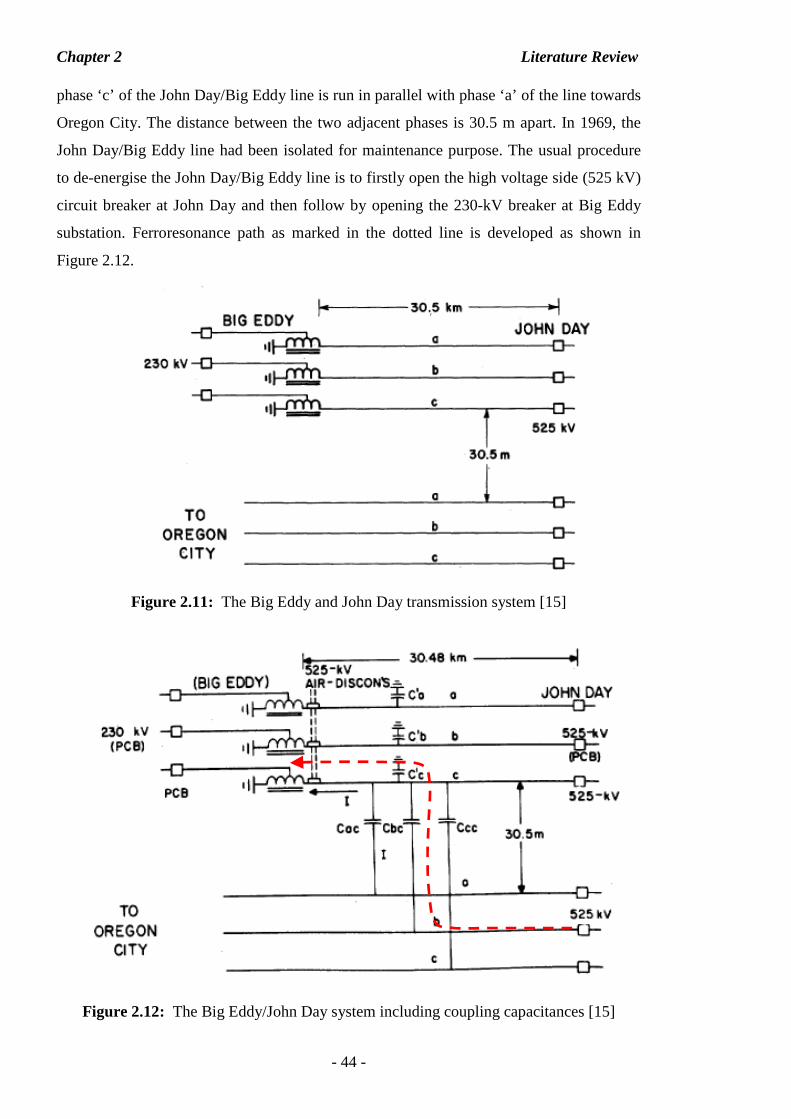
Chapter 2 Literature Review
- 44 -
phase ‘c’ of the John Day/Big Eddy line is run in parallel with phase ‘a’ of the line towards
Oregon City. The distance between the two adjacent phases is 30.5 m apart. In 1969, the
John Day/Big Eddy line had been isolated for maintenance purpose. The usual procedure
to de-energise the John Day/Big Eddy line is to firstly open the high voltage side (525 kV)
circuit breaker at John Day and then follow by opening the 230-kV breaker at Big Eddy
substation. Ferroresonance path as marked in the dotted line is developed as shown in
Figure 2.12.
Figure 2.11: The Big Eddy and John Day transmission system [15]
Figure 2.12: The Big Eddy/John Day system including coupling capacitances [15]
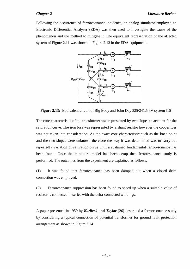
Chapter 2 Literature Review
- 45 -
Following the occurrence of ferroresonance incidence, an analog simulator employed an
Electronic Differential Analyser (EDA) was then used to investigate the cause of the
phenomenon and the method to mitigate it. The equivalent representation of the affected
system of Figure 2.11 was shown in Figure 2.13 in the EDA equipment.
Figure 2.13: Equivalent circuit of Big Eddy and John Day 525/241.5 kV system [15]
The core characteristic of the transformer was represented by two slopes to account for the
saturation curve. The iron loss was represented by a shunt resistor however the copper loss
was not taken into consideration. As the exact core characteristic such as the knee point
and the two slopes were unknown therefore the way it was determined was to carry out
repeatedly variation of saturation curve until a sustained fundamental ferroresonance has
been found. Once the miniature model has been setup then ferroresonance study is
performed. The outcomes from the experiment are explained as follows:
(1) It was found that ferroresonance has been damped out when a closed delta
connection was employed.
(2) Ferroresonance suppression has been found to speed up when a suitable value of
resistor is connected in series with the delta-connected windings.
A paper presented in 1959 by Karlicek and Taylor [26] described a ferroresonance study
by considering a typical connection of potential transformer for ground fault protection
arrangement as shown in Figure 2.14.
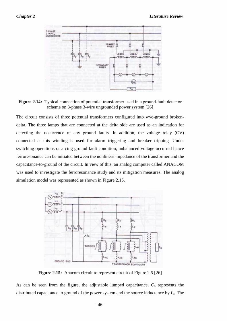
Chapter 2 Literature Review
- 46 -
Figure 2.14: Typical connection of potential transformer used in a ground-fault detector scheme on 3-phase 3-wire ungrounded power system [26]
The circuit consists of three potential transformers configured into wye-ground broken-
delta. The three lamps that are connected at the delta side are used as an indication for
detecting the occurrence of any ground faults. In addition, the voltage relay (CV)
connected at this winding is used for alarm triggering and breaker tripping. Under
switching operations or arcing ground fault condition, unbalanced voltage occurred hence
ferroresonance can be initiated between the nonlinear impedance of the transformer and the
capacitance-to-ground of the circuit. In view of this, an analog computer called ANACOM
was used to investigate the ferroresonance study and its mitigation measures. The analog
simulation model was represented as shown in Figure 2.15.
Figure 2.15: Anacom circuit to represent circuit of Figure 2.5 [26]
As can be seen from the figure, the adjustable lumped capacitance, Co represents the
distributed capacitance to ground of the power system and the source inductance by Ls. The
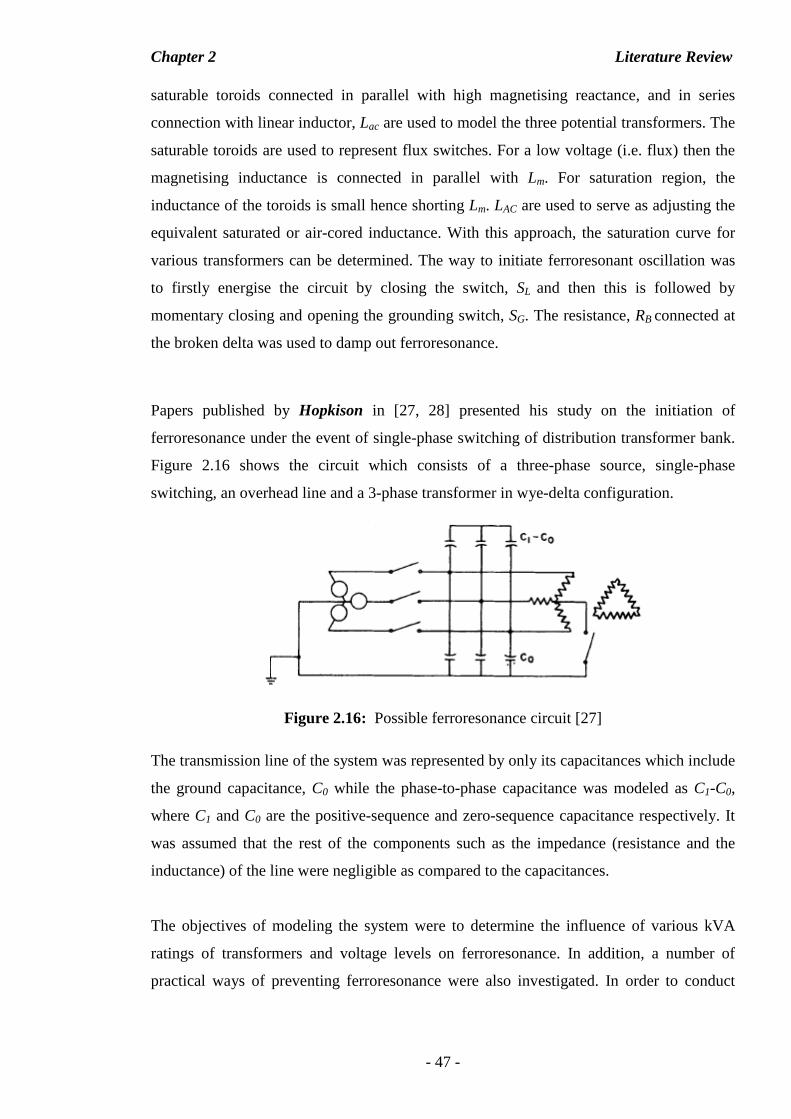
Chapter 2 Literature Review
- 47 -
saturable toroids connected in parallel with high magnetising reactance, and in series
connection with linear inductor, Lac are used to model the three potential transformers. The
saturable toroids are used to represent flux switches. For a low voltage (i.e. flux) then the
magnetising inductance is connected in parallel with Lm. For saturation region, the
inductance of the toroids is small hence shorting Lm. LAC are used to serve as adjusting the
equivalent saturated or air-cored inductance. With this approach, the saturation curve for
various transformers can be determined. The way to initiate ferroresonant oscillation was
to firstly energise the circuit by closing the switch, SL and then this is followed by
momentary closing and opening the grounding switch, SG. The resistance, RB connected at
the broken delta was used to damp out ferroresonance.
Papers published by Hopkison in [27, 28] presented his study on the initiation of
ferroresonance under the event of single-phase switching of distribution transformer bank.
Figure 2.16 shows the circuit which consists of a three-phase source, single-phase
switching, an overhead line and a 3-phase transformer in wye-delta configuration.
Figure 2.16: Possible ferroresonance circuit [27]
The transmission line of the system was represented by only its capacitances which include
the ground capacitance, C0 while the phase-to-phase capacitance was modeled as C1-C0,
where C1 and C0 are the positive-sequence and zero-sequence capacitance respectively. It
was assumed that the rest of the components such as the impedance (resistance and the
inductance) of the line were negligible as compared to the capacitances.
The objectives of modeling the system were to determine the influence of various kVA
ratings of transformers and voltage levels on ferroresonance. In addition, a number of
practical ways of preventing ferroresonance were also investigated. In order to conduct
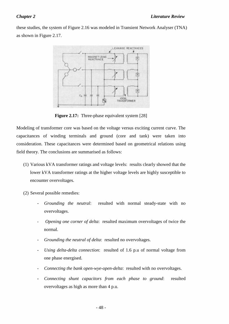
Chapter 2 Literature Review
- 48 -
these studies, the system of Figure 2.16 was modeled in Transient Network Analyser (TNA)
as shown in Figure 2.17.
Figure 2.17: Three-phase equivalent system [28]
Modeling of transformer core was based on the voltage versus exciting current curve. The
capacitances of winding terminals and ground (core and tank) were taken into
consideration. These capacitances were determined based on geometrical relations using
field theory. The conclusions are summarised as follows:
(1) Various kVA transformer ratings and voltage levels: results clearly showed that the
lower kVA transformer ratings at the higher voltage levels are highly susceptible to
encounter overvoltages.
(2) Several possible remedies:
- Grounding the neutral: resulted with normal steady-state with no
overvoltages.
- Opening one corner of delta: resulted maximum overvoltages of twice the
normal.
- Grounding the neutral of delta: resulted no overvoltages.
- Using delta-delta connection: resulted of 1.6 p.u of normal voltage from
one phase energised.
- Connecting the bank open-wye-open-delta: resulted with no overvoltages.
- Connecting shunt capacitors from each phase to ground: resulted
overvoltages as high as more than 4 p.u.
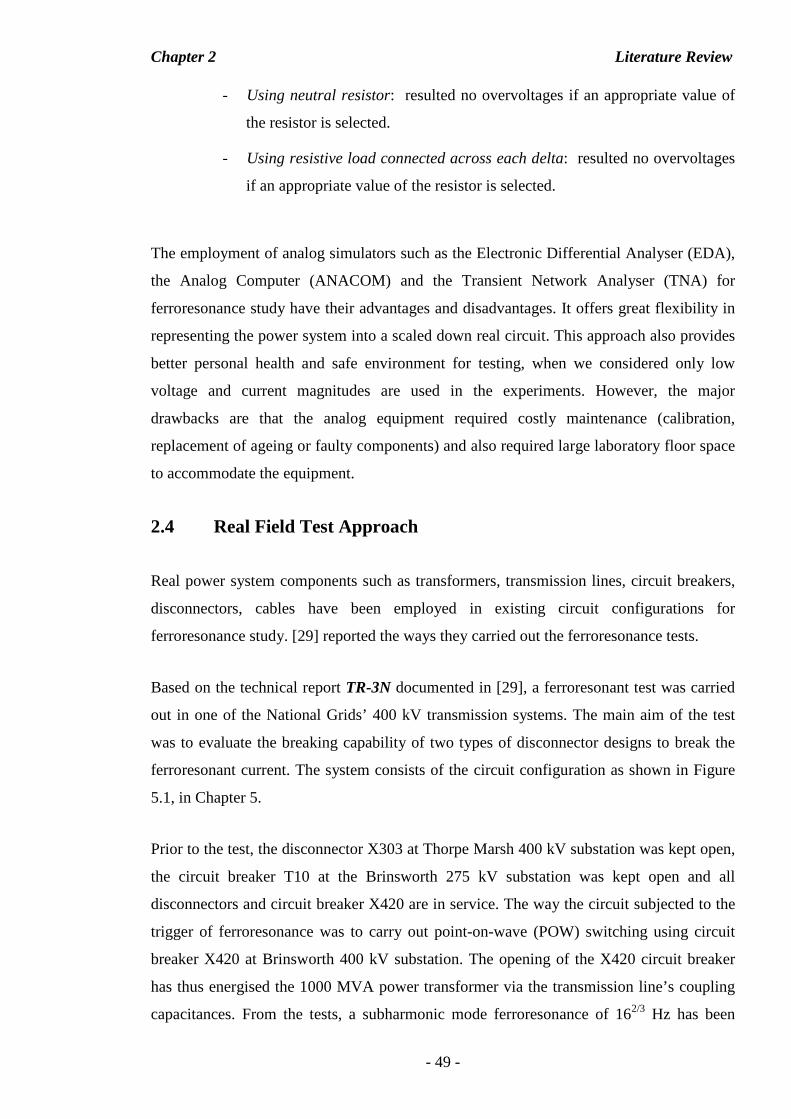
Chapter 2 Literature Review
- 49 -
- Using neutral resistor: resulted no overvoltages if an appropriate value of
the resistor is selected.
- Using resistive load connected across each delta: resulted no overvoltages
if an appropriate value of the resistor is selected.
The employment of analog simulators such as the Electronic Differential Analyser (EDA),
the Analog Computer (ANACOM) and the Transient Network Analyser (TNA) for
ferroresonance study have their advantages and disadvantages. It offers great flexibility in
representing the power system into a scaled down real circuit. This approach also provides
better personal health and safe environment for testing, when we considered only low
voltage and current magnitudes are used in the experiments. However, the major
drawbacks are that the analog equipment required costly maintenance (calibration,
replacement of ageing or faulty components) and also required large laboratory floor space
to accommodate the equipment.
2.4 Real Field Test Approach
Real power system components such as transformers, transmission lines, circuit breakers,
disconnectors, cables have been employed in existing circuit configurations for
ferroresonance study. [29] reported the ways they carried out the ferroresonance tests.
Based on the technical report TR-3N documented in [29], a ferroresonant test was carried
out in one of the National Grids’ 400 kV transmission systems. The main aim of the test
was to evaluate the breaking capability of two types of disconnector designs to break the
ferroresonant current. The system consists of the circuit configuration as shown in Figure
5.1, in Chapter 5.
Prior to the test, the disconnector X303 at Thorpe Marsh 400 kV substation was kept open,
the circuit breaker T10 at the Brinsworth 275 kV substation was kept open and all
disconnectors and circuit breaker X420 are in service. The way the circuit subjected to the
trigger of ferroresonance was to carry out point-on-wave (POW) switching using circuit
breaker X420 at Brinsworth 400 kV substation. The opening of the X420 circuit breaker
has thus energised the 1000 MVA power transformer via the transmission line’s coupling
capacitances. From the tests, a subharmonic mode ferroresonance of 162/3 Hz has been
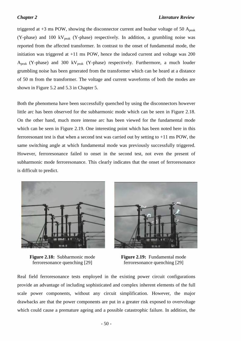
Chapter 2 Literature Review
- 50 -
triggered at +3 ms POW, showing the disconnector current and busbar voltage of 50 Apeak
(Y-phase) and 100 kVpeak (Y-phase) respectively. In addition, a grumbling noise was
reported from the affected transformer. In contrast to the onset of fundamental mode, the
initiation was triggered at +11 ms POW, hence the induced current and voltage was 200
Apeak (Y-phase) and 300 kVpeak (Y-phase) respectively. Furthermore, a much louder
grumbling noise has been generated from the transformer which can be heard at a distance
of 50 m from the transformer. The voltage and current waveforms of both the modes are
shown in Figure 5.2 and 5.3 in Chapter 5.
Both the phenomena have been successfully quenched by using the disconnectors however
little arc has been observed for the subharmonic mode which can be seen in Figure 2.18.
On the other hand, much more intense arc has been viewed for the fundamental mode
which can be seen in Figure 2.19. One interesting point which has been noted here in this
ferroresonant test is that when a second test was carried out by setting to +11 ms POW, the
same switching angle at which fundamental mode was previously successfully triggered.
However, ferroresonance failed to onset in the second test, not even the present of
subharmonic mode ferroresonance. This clearly indicates that the onset of ferroresonance
is difficult to predict.
Figure 2.18: Subharmonic mode ferroresonance quenching [29]
Figure 2.19: Fundamental mode ferroresonance quenching [29]
Real field ferroresonance tests employed in the existing power circuit configurations
provide an advantage of including sophisticated and complex inherent elements of the full
scale power components, without any circuit simplification. However, the major
drawbacks are that the power components are put in a greater risk exposed to overvoltage
which could cause a premature ageing and a possible catastrophic failure. In addition, the
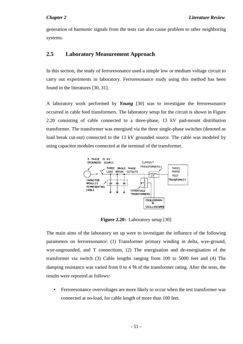
Chapter 2 Literature Review
- 51 -
generation of harmonic signals from the tests can also cause problem to other neighboring
systems.
2.5 Laboratory Measurement Approach
In this section, the study of ferroresonance used a simple low or medium voltage circuit to
carry out experiments in laboratory. Ferroresonance study using this method has been
found in the literatures [30, 31].
A laboratory work performed by Young [30] was to investigate the ferroresonance
occurred in cable feed transformers. The laboratory setup for the circuit is shown in Figure
2.20 consisting of cable connected to a three-phase, 13 kV pad-mount distribution
transformer. The transformer was energised via the three single-phase switches (denoted as
load break cut-out) connected to the 13 kV grounded source. The cable was modeled by
using capacitor modules connected at the terminal of the transformer.
Figure 2.20: Laboratory setup [30]
The main aims of the laboratory set up were to investigate the influence of the following
parameters on ferroresonance: (1) Transformer primary winding in delta, wye-ground,
wye-ungrounded, and T connections, (2) The energisation and de-energisation of the
transformer via switch (3) Cable lengths ranging from 100 to 5000 feet and (4) The
damping resistance was varied from 0 to 4 % of the transformer rating. After the tests, the
results were reported as follows:
• Ferroresonance overvoltages are more likely to occur when the test transformer was
connected at no-load, for cable length of more than 100 feet.
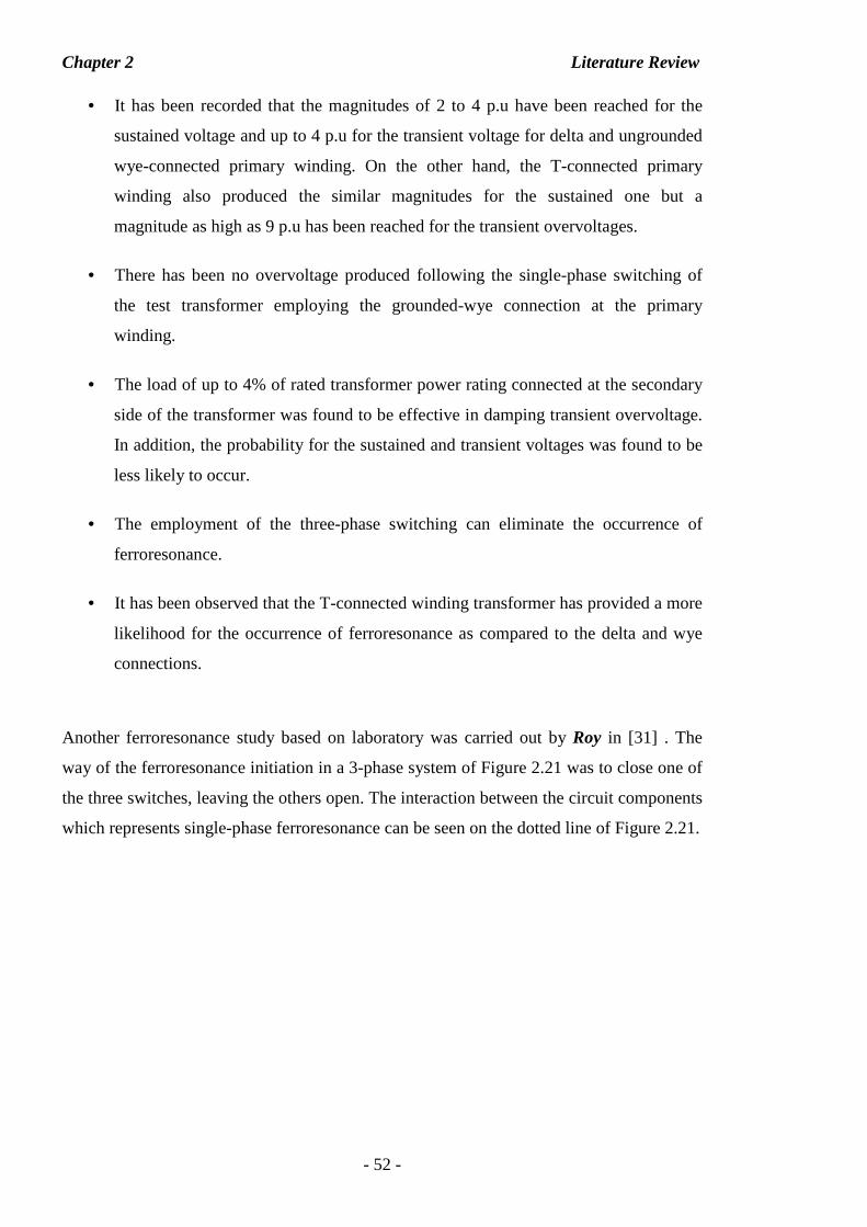
Chapter 2 Literature Review
- 52 -
• It has been recorded that the magnitudes of 2 to 4 p.u have been reached for the
sustained voltage and up to 4 p.u for the transient voltage for delta and ungrounded
wye-connected primary winding. On the other hand, the T-connected primary
winding also produced the similar magnitudes for the sustained one but a
magnitude as high as 9 p.u has been reached for the transient overvoltages.
• There has been no overvoltage produced following the single-phase switching of
the test transformer employing the grounded-wye connection at the primary
winding.
• The load of up to 4% of rated transformer power rating connected at the secondary
side of the transformer was found to be effective in damping transient overvoltage.
In addition, the probability for the sustained and transient voltages was found to be
less likely to occur.
• The employment of the three-phase switching can eliminate the occurrence of
ferroresonance.
• It has been observed that the T-connected winding transformer has provided a more
likelihood for the occurrence of ferroresonance as compared to the delta and wye
connections.
Another ferroresonance study based on laboratory was carried out by Roy in [31] . The
way of the ferroresonance initiation in a 3-phase system of Figure 2.21 was to close one of
the three switches, leaving the others open. The interaction between the circuit components
which represents single-phase ferroresonance can be seen on the dotted line of Figure 2.21.
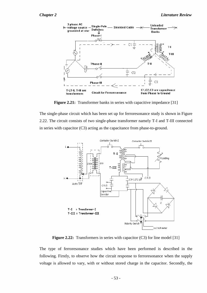
Chapter 2 Literature Review
- 53 -
Figure 2.21: Transformer banks in series with capacitive impedance [31]
The single-phase circuit which has been set up for ferroresonance study is shown in Figure
2.22. The circuit consists of two single-phase transformer namely T-I and T-III connected
in series with capacitor (C3) acting as the capacitance from phase-to-ground.
Figure 2.22: Transformers in series with capacitor (C3) for line model [31]
The type of ferroresonance studies which have been performed is described in the
following. Firstly, to observe how the circuit response to ferroresonance when the supply
voltage is allowed to vary, with or without stored charge in the capacitor. Secondly, the
Chapter 2 Literature Review
- 54 -
study with supply voltage fixed at 100% of the rated transformer with negative stored
charges presents in the capacitor. Thirdly, the study of mitigation of ferroresonance by
using damping resistor connected at the secondary side of the transformer. Finally, an
interruption of short-circuit study was conducted by overloading the system with low
resistance connected at the secondary side of the transformer. The results from the
experiment are explained as follows:
(1) Supply voltage is varied:
- Capacitor without stored charge: Resulted no ferroresonance when the supply is
80% of the rated value of transformer. Sustained ferroresonance of 5.8 p.u occurred when
the supply is 100% of the rated value of transformer.
- Capacitor with negative stored charge: It has resulted in a situation where capacitor
voltage increased asymmetrically with positive value and approaching to a damaging
voltage of 7.44 p.u.
- Capacitor with positive stored charge: This has resulted in the capacitor voltage
being increased asymmetrically with negative amplitude of -7.31 p.u.
(2) Mitigation of ferroresonance by using damping resistor connected at the secondary
side of the transformer
- Initial stored charge = 0 V, applied voltage = 92% of rated transformer: Initially,
the ferroresonance has damped out when a load is applied at the secondary winding of the
transformer but it reoccurs again when the load is removed from the transformer.
- Initial stored charge = positive, applied voltage = 92% of rated transformer: Even
with the presence of the initial positive charge in the capacitor, the damping resistor will
still be able to provide the damping effect. However, ferroresonance again re-built after
removal of the resistor from the transformer.
(3) Interruption of short-circuit study by overloading the system with low resistance
connected at the secondary side of the transformer
- A transient overvoltage of 4.11 p.u peak and then a sustained steady state voltage of
3.04 p.u have been noted before the fault has been interrupted. A sustained ferroresonance
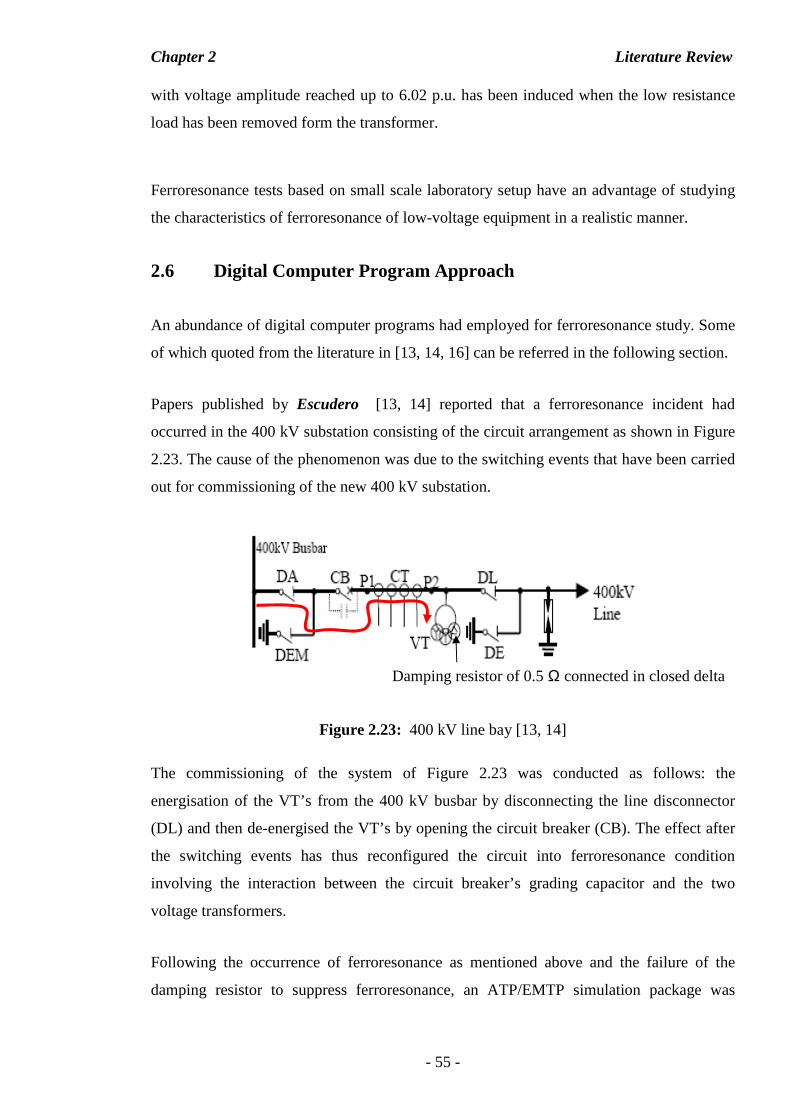
Chapter 2 Literature Review
- 55 -
with voltage amplitude reached up to 6.02 p.u. has been induced when the low resistance
load has been removed form the transformer.
Ferroresonance tests based on small scale laboratory setup have an advantage of studying
the characteristics of ferroresonance of low-voltage equipment in a realistic manner.
2.6 Digital Computer Program Approach
An abundance of digital computer programs had employed for ferroresonance study. Some
of which quoted from the literature in [13, 14, 16] can be referred in the following section.
Papers published by Escudero [13, 14] reported that a ferroresonance incident had
occurred in the 400 kV substation consisting of the circuit arrangement as shown in Figure
2.23. The cause of the phenomenon was due to the switching events that have been carried
out for commissioning of the new 400 kV substation.
Figure 2.23: 400 kV line bay [13, 14]
The commissioning of the system of Figure 2.23 was conducted as follows: the
energisation of the VT’s from the 400 kV busbar by disconnecting the line disconnector
(DL) and then de-energised the VT’s by opening the circuit breaker (CB). The effect after
the switching events has thus reconfigured the circuit into ferroresonance condition
involving the interaction between the circuit breaker’s grading capacitor and the two
voltage transformers.
Following the occurrence of ferroresonance as mentioned above and the failure of the
damping resistor to suppress ferroresonance, an ATP/EMTP simulation package was
Damping resistor of 0.5 Ω connected in closed delta
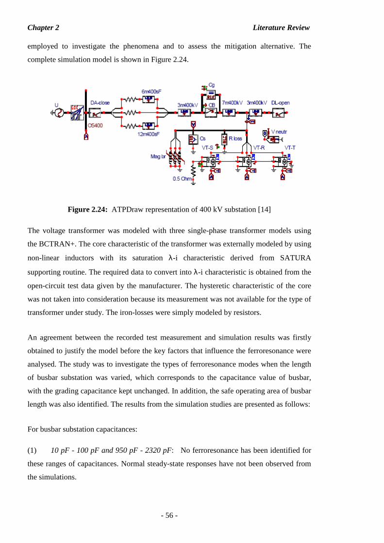
Chapter 2 Literature Review
- 56 -
employed to investigate the phenomena and to assess the mitigation alternative. The
complete simulation model is shown in Figure 2.24.
Figure 2.24: ATPDraw representation of 400 kV substation [14]
The voltage transformer was modeled with three single-phase transformer models using
the BCTRAN+. The core characteristic of the transformer was externally modeled by using
non-linear inductors with its saturation λ-i characteristic derived from SATURA
supporting routine. The required data to convert into λ-i characteristic is obtained from the
open-circuit test data given by the manufacturer. The hysteretic characteristic of the core
was not taken into consideration because its measurement was not available for the type of
transformer under study. The iron-losses were simply modeled by resistors.
An agreement between the recorded test measurement and simulation results was firstly
obtained to justify the model before the key factors that influence the ferroresonance were
analysed. The study was to investigate the types of ferroresonance modes when the length
of busbar substation was varied, which corresponds to the capacitance value of busbar,
with the grading capacitance kept unchanged. In addition, the safe operating area of busbar
length was also identified. The results from the simulation studies are presented as follows:
For busbar substation capacitances:
(1) 10 pF - 100 pF and 950 pF - 2320 pF: No ferroresonance has been identified for
these ranges of capacitances. Normal steady-state responses have not been observed from
the simulations.
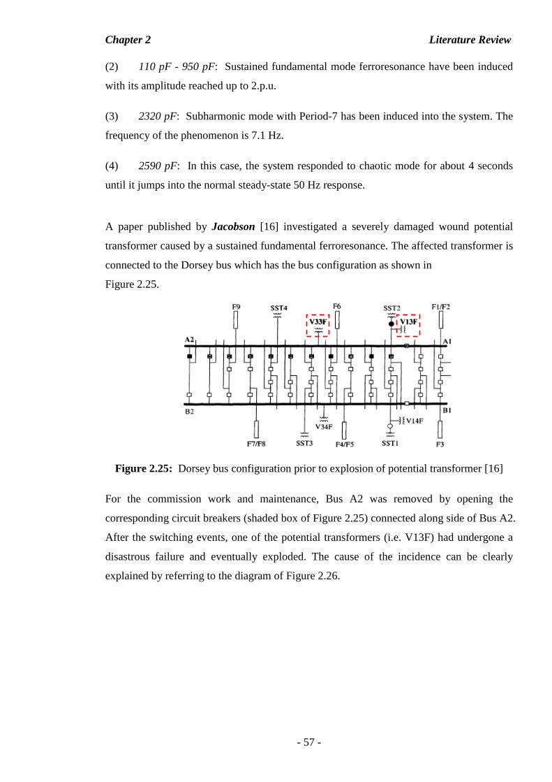
Chapter 2 Literature Review
- 57 -
(2) 110 pF - 950 pF: Sustained fundamental mode ferroresonance have been induced
with its amplitude reached up to 2.p.u.
(3) 2320 pF: Subharmonic mode with Period-7 has been induced into the system. The
frequency of the phenomenon is 7.1 Hz.
(4) 2590 pF: In this case, the system responded to chaotic mode for about 4 seconds
until it jumps into the normal steady-state 50 Hz response.
A paper published by Jacobson [16] investigated a severely damaged wound potential
transformer caused by a sustained fundamental ferroresonance. The affected transformer is
connected to the Dorsey bus which has the bus configuration as shown in
Figure 2.25.
Figure 2.25: Dorsey bus configuration prior to explosion of potential transformer [16]
For the commission work and maintenance, Bus A2 was removed by opening the
corresponding circuit breakers (shaded box of Figure 2.25) connected along side of Bus A2.
After the switching events, one of the potential transformers (i.e. V13F) had undergone a
disastrous failure and eventually exploded. The cause of the incidence can be clearly
explained by referring to the diagram of Figure 2.26.
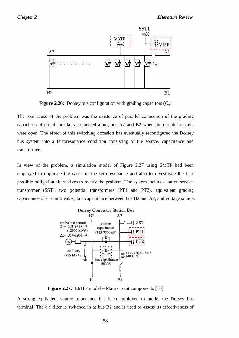
Chapter 2 Literature Review
- 58 -
Figure 2.26: Dorsey bus configuration with grading capacitors (Cg)
The root cause of the problem was the existence of parallel connection of the grading
capacitors of circuit breakers connected along bus A2 and B2 when the circuit breakers
were open. The effect of this switching occasion has eventually reconfigured the Dorsey
bus system into a ferroresonance condition consisting of the source, capacitance and
transformers.
In view of the problem, a simulation model of Figure 2.27 using EMTP had been
employed to duplicate the cause of the ferroresonance and also to investigate the best
possible mitigation alternatives to rectify the problem. The system includes station service
transformer (SST), two potential transformers (PT1 and PT2), equivalent grading
capacitance of circuit breaker, bus capacitance between bus B2 and A2, and voltage source.
Figure 2.27: EMTP model – Main circuit components [16]
A strong equivalent source impedance has been employed to model the Dorsey bus
terminal. The a.c filter is switched in at bus B2 and is used to assess its effectiveness of
V13F
. . . . . . . . . .
A2
B2
Cg
A1
V33F
B1
SST1
. . . . . . . . . .
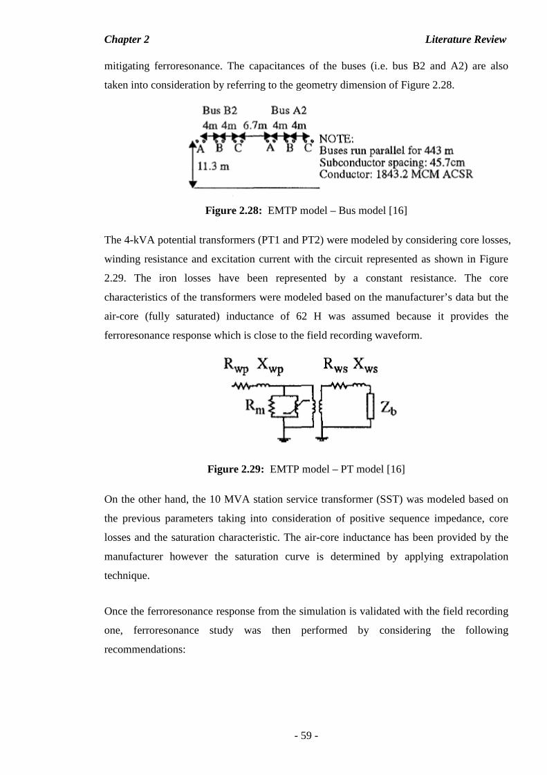
Chapter 2 Literature Review
- 59 -
mitigating ferroresonance. The capacitances of the buses (i.e. bus B2 and A2) are also
taken into consideration by referring to the geometry dimension of Figure 2.28.
Figure 2.28: EMTP model – Bus model [16]
The 4-kVA potential transformers (PT1 and PT2) were modeled by considering core losses,
winding resistance and excitation current with the circuit represented as shown in Figure
2.29. The iron losses have been represented by a constant resistance. The core
characteristics of the transformers were modeled based on the manufacturer’s data but the
air-core (fully saturated) inductance of 62 H was assumed because it provides the
ferroresonance response which is close to the field recording waveform.
Figure 2.29: EMTP model – PT model [16]
On the other hand, the 10 MVA station service transformer (SST) was modeled based on
the previous parameters taking into consideration of positive sequence impedance, core
losses and the saturation characteristic. The air-core inductance has been provided by the
manufacturer however the saturation curve is determined by applying extrapolation
technique.
Once the ferroresonance response from the simulation is validated with the field recording
one, ferroresonance study was then performed by considering the following
recommendations:
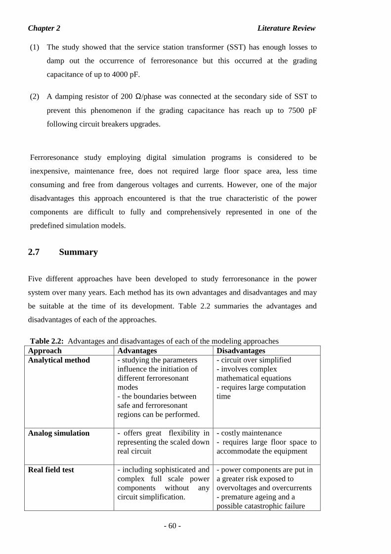
Chapter 2 Literature Review
- 60 -
(1) The study showed that the service station transformer (SST) has enough losses to
damp out the occurrence of ferroresonance but this occurred at the grading
capacitance of up to 4000 pF.
(2) A damping resistor of 200 Ω/phase was connected at the secondary side of SST to
prevent this phenomenon if the grading capacitance has reach up to 7500 pF
following circuit breakers upgrades.
Ferroresonance study employing digital simulation programs is considered to be
inexpensive, maintenance free, does not required large floor space area, less time
consuming and free from dangerous voltages and currents. However, one of the major
disadvantages this approach encountered is that the true characteristic of the power
components are difficult to fully and comprehensively represented in one of the
predefined simulation models.
2.7 Summary
Five different approaches have been developed to study ferroresonance in the power
system over many years. Each method has its own advantages and disadvantages and may
be suitable at the time of its development. Table 2.2 summaries the advantages and
disadvantages of each of the approaches.
Table 2.2: Advantages and disadvantages of each of the modeling approaches Approach Advantages Disadvantages Analytical method - studying the parameters
influence the initiation of different ferroresonant modes - the boundaries between safe and ferroresonant regions can be performed.
- circuit over simplified - involves complex mathematical equations - requires large computation time
Analog simulation - offers great flexibility in representing the scaled down real circuit
- costly maintenance - requires large floor space to accommodate the equipment
Real field test - including sophisticated and complex full scale power components without any circuit simplification.
- power components are put in a greater risk exposed to overvoltages and overcurrents - premature ageing and a possible catastrophic failure
Chapter 2 Literature Review
- 61 -
Laboratory measurement
- studying the characteristics of ferroresonance of low-voltage equipment in a realistic manner
Digital computer program
- inexpensive, maintenance free, does not required large floor area, less time consuming - free from dangerous overvoltages and overcurrents
- power system components are difficult to fully and comprehensively represented in a predefined simulation model alone.
.
In view of the computation power of modern computer and well-developed power system
transient softwares, the current approach used in this thesis is to carry out simulation
studies for understanding the network transients performance, to aid network design and to
analyse the failure causes in the existing system.
Chapter 3 Single-Phase Ferroresonance – A Case Study
- 62 -
CHAPTER 3 CHAPTER 3 CHAPTER 3 CHAPTER 3
333... SSSIII NNNGGGLLL EEE---PPPHHHAAASSSEEE FFFEEERRRRRROOORRREEESSSOOONNNAAANNNCCCEEE ––– AAA CCCAAASSSEEE SSSTTTUUUDDDYYY
3.1 Introduction
Ferroresonance has been identified as a nonlinear event which can cause damaging of
power system equipment as a result of exhibiting overvoltages and overcurrents. In view of
this, power network must function beyond the boundary of ferroresonant regions, and in
addition minimise the likelihood of occurrence of such response when planning of
expansion of network takes place. In order to achieve this, a comprehensive understanding
of such phenomenon is essential for power system engineers, that is by looking into the
variations of system parameters and transformer parameters which are known to directly
influence ferroresonance response so as to gain a better understanding about its behaviour.
As an initial stage of the current study, a single-phase ferroresonance equivalent circuit
employing a potential transformer (PT) quoted in [16] is used as a case study. The studies
aim to achieve the goals as follows:
(1) Identification of ferroresonant modes such as sustained fundamental, quasi-
subharmonic, subharmonic and chaotic modes by varying both the grading and shunt
capacitances for both high and low core nonlinearity characteristics.
(2) Suppression of sustained fundamental ferroresonant mode by having variation of
core-losses introduced into the transformer core characteristic.
(3) Recognising the key parameters for providing initiation and sustainability of
ferroresonance, particularly the sustained fundamental mode.
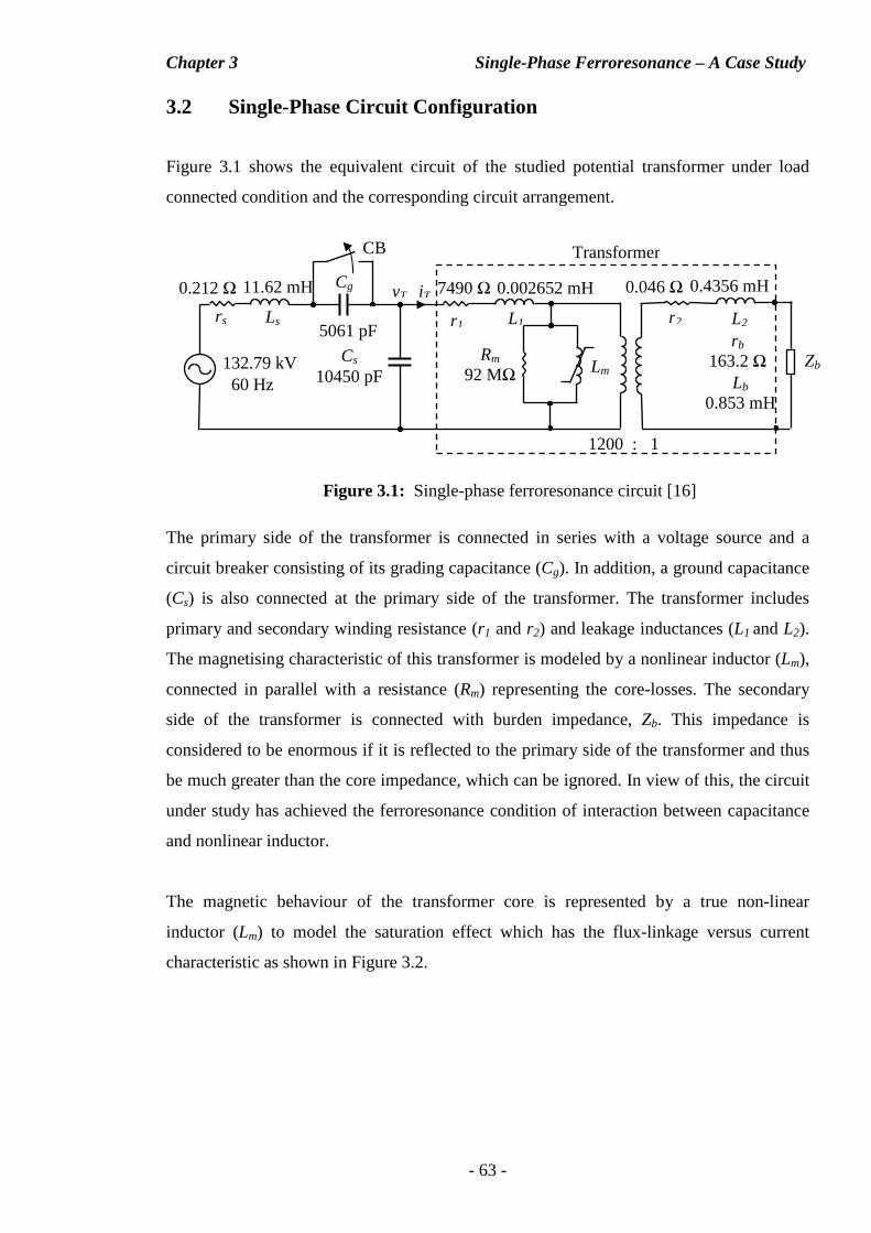
Chapter 3 Single-Phase Ferroresonance – A Case Study
- 63 -
3.2 Single-Phase Circuit Configuration
Figure 3.1 shows the equivalent circuit of the studied potential transformer under load
connected condition and the corresponding circuit arrangement.
Figure 3.1: Single-phase ferroresonance circuit [16]
The primary side of the transformer is connected in series with a voltage source and a
circuit breaker consisting of its grading capacitance (Cg). In addition, a ground capacitance
(Cs) is also connected at the primary side of the transformer. The transformer includes
primary and secondary winding resistance (r1 and r2) and leakage inductances (L1 and L2).
The magnetising characteristic of this transformer is modeled by a nonlinear inductor (Lm),
connected in parallel with a resistance (Rm) representing the core-losses. The secondary
side of the transformer is connected with burden impedance, Zb. This impedance is
considered to be enormous if it is reflected to the primary side of the transformer and thus
be much greater than the core impedance, which can be ignored. In view of this, the circuit
under study has achieved the ferroresonance condition of interaction between capacitance
and nonlinear inductor.
The magnetic behaviour of the transformer core is represented by a true non-linear
inductor (Lm) to model the saturation effect which has the flux-linkage versus current
characteristic as shown in Figure 3.2.
r1 L1
Rm
92 MΩ
1200 : 1
Lm
Transformer
Zb
r2 L2
CB
vT
Cs 10450 pF
Cg
rs Ls
iT 0.212 Ω 11.62 mH 7490 Ω 0.002652 mH
5061 pF
0.046 Ω 0.4356 mH
rb
163.2 Ω
Lb
0.853 mH
132.79 kV 60 Hz
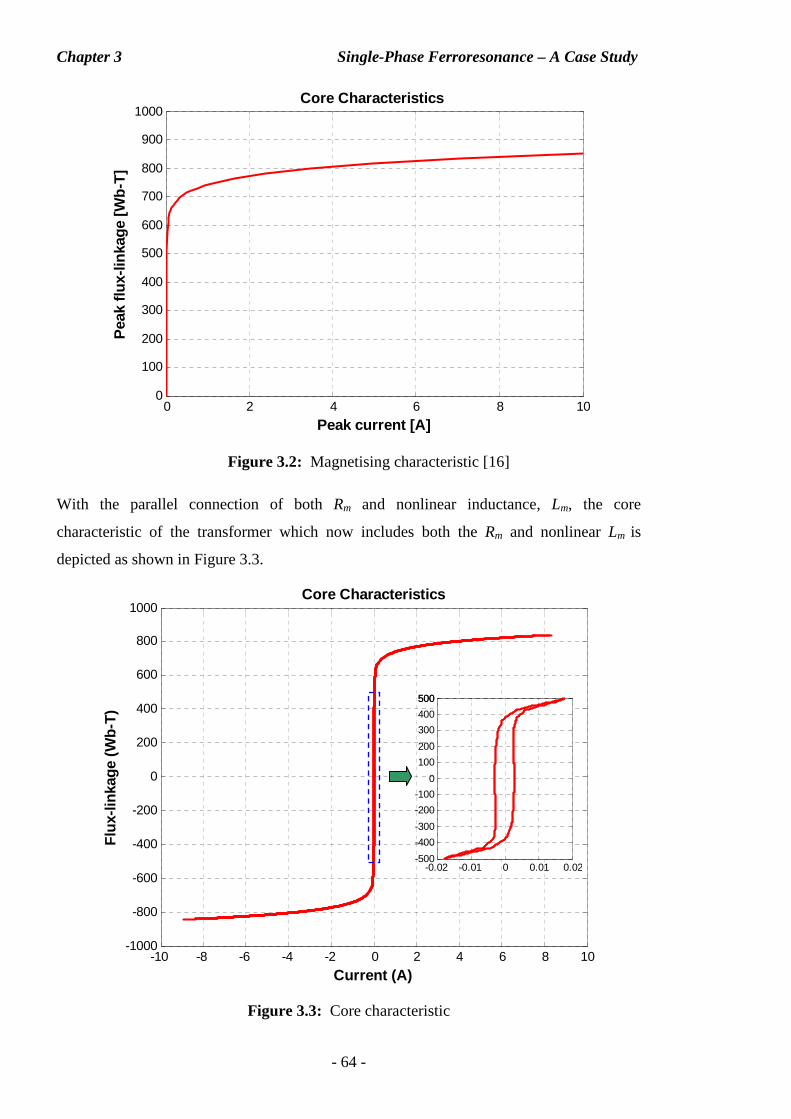
Chapter 3 Single-Phase Ferroresonance – A Case Study
- 64 -
Figure 3.2: Magnetising characteristic [16]
With the parallel connection of both Rm and nonlinear inductance, Lm, the core
characteristic of the transformer which now includes both the Rm and nonlinear Lm is
depicted as shown in Figure 3.3.
Figure 3.3: Core characteristic
-10 -8 -6 -4 -2 0 2 4 6 8 10-1000
-800
-600
-400
-200
0
200
400
600
800
1000Core Characteristics
Current (A)
Flu
x-lin
kage
(W
b-T
)
-0.02 -0.01 0 0.01 0.02-500
-400
-300
-200
-100
0
100
200
300
400
500500
0 2 4 6 8 100
100
200
300
400
500
600
700
800
900
1000Core Characteristics
Pea
k flu
x-lin
kage
[Wb-
T]
Peak current [A]
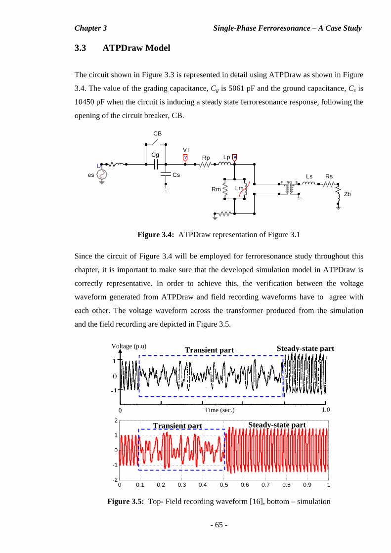
Chapter 3 Single-Phase Ferroresonance – A Case Study
- 65 -
3.3 ATPDraw Model
The circuit shown in Figure 3.3 is represented in detail using ATPDraw as shown in Figure
3.4. The value of the grading capacitance, Cg is 5061 pF and the ground capacitance, Cs is
10450 pF when the circuit is inducing a steady state ferroresonance response, following the
opening of the circuit breaker, CB.
Figure 3.4: ATPDraw representation of Figure 3.1
Since the circuit of Figure 3.4 will be employed for ferroresonance study throughout this
chapter, it is important to make sure that the developed simulation model in ATPDraw is
correctly representative. In order to achieve this, the verification between the voltage
waveform generated from ATPDraw and field recording waveforms have to agree with
each other. The voltage waveform across the transformer produced from the simulation
and the field recording are depicted in Figure 3.5.
Figure 3.5: Top- Field recording waveform [16], bottom – simulation
U
V VRp Lp
RsLs
ZbRm Lm
Cg
CB
es Cs
VT
0
1
0 1.0 Time (sec.)
-1
0
Voltage (p.u) Transient part Steady-state part
0 0.1 0.2 0.3 0.4 0.5 0.6 0.7 0.8 0.9 1-2
-1
0
1
2Transient part Steady-state part
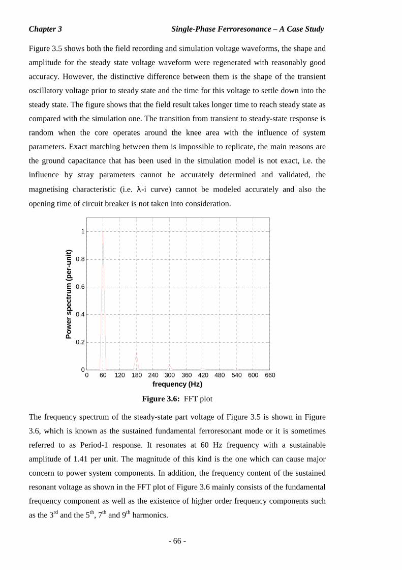
Chapter 3 Single-Phase Ferroresonance – A Case Study
- 66 -
Figure 3.5 shows both the field recording and simulation voltage waveforms, the shape and
amplitude for the steady state voltage waveform were regenerated with reasonably good
accuracy. However, the distinctive difference between them is the shape of the transient
oscillatory voltage prior to steady state and the time for this voltage to settle down into the
steady state. The figure shows that the field result takes longer time to reach steady state as
compared with the simulation one. The transition from transient to steady-state response is
random when the core operates around the knee area with the influence of system
parameters. Exact matching between them is impossible to replicate, the main reasons are
the ground capacitance that has been used in the simulation model is not exact, i.e. the
influence by stray parameters cannot be accurately determined and validated, the
magnetising characteristic (i.e. λ-i curve) cannot be modeled accurately and also the
opening time of circuit breaker is not taken into consideration.
Figure 3.6: FFT plot
The frequency spectrum of the steady-state part voltage of Figure 3.5 is shown in Figure
3.6, which is known as the sustained fundamental ferroresonant mode or it is sometimes
referred to as Period-1 response. It resonates at 60 Hz frequency with a sustainable
amplitude of 1.41 per unit. The magnitude of this kind is the one which can cause major
concern to power system components. In addition, the frequency content of the sustained
resonant voltage as shown in the FFT plot of Figure 3.6 mainly consists of the fundamental
frequency component as well as the existence of higher order frequency components such
as the 3rd and the 5th, 7th and 9th harmonics.
0 60 120 180 240 300 360 420 480 540 600 6600
0.2
0.4
0.6
0.8
1
frequency (Hz)
Pow
er s
pect
rum
(pe
r-un
it)
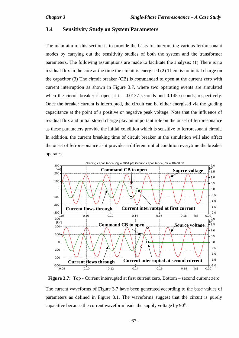
Chapter 3 Single-Phase Ferroresonance – A Case Study
- 67 -
3.4 Sensitivity Study on System Parameters
The main aim of this section is to provide the basis for interpreting various ferroresonant
modes by carrying out the sensitivity studies of both the system and the transformer
parameters. The following assumptions are made to facilitate the analysis: (1) There is no
residual flux in the core at the time the circuit is energised (2) There is no initial charge on
the capacitor (3) The circuit breaker (CB) is commanded to open at the current zero with
current interruption as shown in Figure 3.7, where two operating events are simulated
when the circuit breaker is open at t = 0.0137 seconds and 0.145 seconds, respectively.
Once the breaker current is interrupted, the circuit can be either energised via the grading
capacitance at the point of a positive or negative peak voltage. Note that the influence of
residual flux and initial stored charge play an important role on the onset of ferroresonance
as these parameters provide the initial condition which is sensitive to ferroresonant circuit.
In addition, the current breaking time of circuit breaker in the simulation will also affect
the onset of ferroresonance as it provides a different initial condition everytime the breaker
operates.
Figure 3.7: Top - Current interrupted at first current zero, Bottom – second current zero
The current waveforms of Figure 3.7 have been generated according to the base values of
parameters as defined in Figure 3.1. The waveforms suggest that the circuit is purely
capacitive because the current waveform leads the supply voltage by 90o.
0.08 0.10 0.12 0.14 0.16 0.18 0.20[s]-300
-200
-100
0
100
200
300[kV]
-2.0
-1.5
-1.0
-0.5
0.0
0.5
1.0
1.5
2.0[A]
0.08 0.10 0.12 0.14 0.16 0.18 0.20[s]-300
-200
-100
0
100
200
300[kV]
-2.0
-1.5
-1.0
-0.5
0.0
0.5
1.0
1.5
2.0[A]
Grading capacitance, Cg = 5061 pF, Ground capacitance, Cs = 10450 pF
Command CB to open
Current interrupted at first current Current flows through
Source voltage
Current interrupted at second current zero
Current flows through
Source voltage Command CB to open
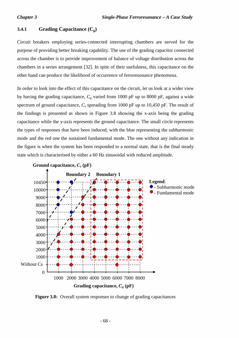
Chapter 3 Single-Phase Ferroresonance – A Case Study
- 68 -
3.4.1 Grading Capacitance (Cg)
Circuit breakers employing series-connected interrupting chambers are served for the
purpose of providing better breaking capability. The use of the grading capacitor connected
across the chamber is to provide improvement of balance of voltage distribution across the
chambers in a series arrangement [32]. In spite of their usefulness, this capacitance on the
other hand can produce the likelihood of occurrence of ferroresonance phenomena.
In order to look into the effect of this capacitance on the circuit, let us look at a wider view
by having the grading capacitance, Cg varied from 1000 pF up to 8000 pF, against a wide
spectrum of ground capacitance, Cs spreading from 1000 pF up to 10,450 pF. The result of
the findings is presented as shown in Figure 3.8 showing the x-axis being the grading
capacitance while the y-axis represents the ground capacitance. The small circle represents
the types of responses that have been induced, with the blue representing the subharmonic
mode and the red one the sustained fundamental mode. The one without any indication in
the figure is when the system has been responded to a normal state, that is the final steady
state which is characterised by either a 60 Hz sinusoidal with reduced amplitude.
Figure 3.8: Overall system responses to change of grading capacitances
Ground capacitance, Cs (pF)
Without Cs
Grading capacitance, Cg (pF)
Legend: - Subharmonic mode - Fundamental mode
0
1000
1000 2000 3000 4000 5000 6000 7000 8000
2000
3000
4000
5000
6000
7000
8000
9000
10000
10450
Boundary 1 Boundary 2
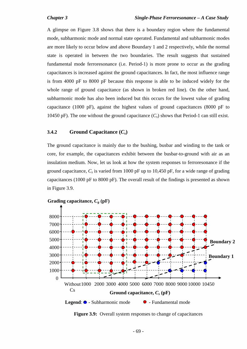
Chapter 3 Single-Phase Ferroresonance – A Case Study
- 69 -
A glimpse on Figure 3.8 shows that there is a boundary region where the fundamental
mode, subharmonic mode and normal state operated. Fundamental and subharmonic modes
are more likely to occur below and above Boundary 1 and 2 respectively, while the normal
state is operated in between the two boundaries. The result suggests that sustained
fundamental mode ferroresonance (i.e. Period-1) is more prone to occur as the grading
capacitances is increased against the ground capacitances. In fact, the most influence range
is from 4000 pF to 8000 pF because this response is able to be induced widely for the
whole range of ground capacitance (as shown in broken red line). On the other hand,
subharmonic mode has also been induced but this occurs for the lowest value of grading
capacitance (1000 pF), against the highest values of ground capacitances (8000 pF to
10450 pF). The one without the ground capacitance (Cs) shows that Period-1 can still exist.
3.4.2 Ground Capacitance (Cs)
The ground capacitance is mainly due to the bushing, busbar and winding to the tank or
core, for example, the capacitances exhibit between the busbar-to-ground with air as an
insulation medium. Now, let us look at how the system responses to ferroresonance if the
ground capacitance, Cs is varied from 1000 pF up to 10,450 pF, for a wide range of grading
capacitances (1000 pF to 8000 pF). The overall result of the findings is presented as shown
in Figure 3.9.
Figure 3.9: Overall system responses to change of capacitances
Legend: - Subharmonic mode - Fundamental mode
Grading capacitance, Cg (pF)
0
1000
2000
3000
4000
5000
6000
7000
8000
1000 2000 3000 4000 5000 6000 7000 8000 9000 10000 10450 Without Cs Ground capacitance, Cs (pF)
Boundary 1
Boundary 2
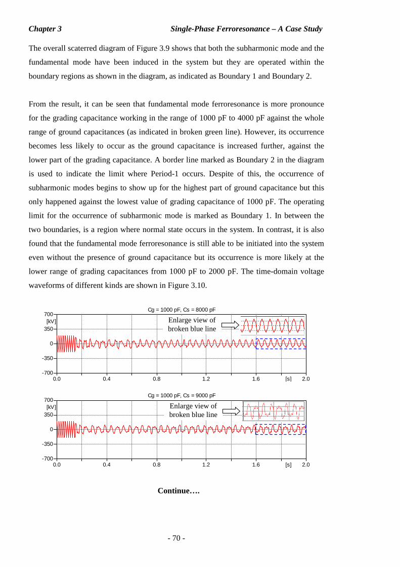
Chapter 3 Single-Phase Ferroresonance – A Case Study
- 70 -
The overall scaterred diagram of Figure 3.9 shows that both the subharmonic mode and the
fundamental mode have been induced in the system but they are operated within the
boundary regions as shown in the diagram, as indicated as Boundary 1 and Boundary 2.
From the result, it can be seen that fundamental mode ferroresonance is more pronounce
for the grading capacitance working in the range of 1000 pF to 4000 pF against the whole
range of ground capacitances (as indicated in broken green line). However, its occurrence
becomes less likely to occur as the ground capacitance is increased further, against the
lower part of the grading capacitance. A border line marked as Boundary 2 in the diagram
is used to indicate the limit where Period-1 occurs. Despite of this, the occurrence of
subharmonic modes begins to show up for the highest part of ground capacitance but this
only happened against the lowest value of grading capacitance of 1000 pF. The operating
limit for the occurrence of subharmonic mode is marked as Boundary 1. In between the
two boundaries, is a region where normal state occurs in the system. In contrast, it is also
found that the fundamental mode ferroresonance is still able to be initiated into the system
even without the presence of ground capacitance but its occurrence is more likely at the
lower range of grading capacitances from 1000 pF to 2000 pF. The time-domain voltage
waveforms of different kinds are shown in Figure 3.10.
0.0 0.4 0.8 1.2 1.6 2.0[s]-700
-350
0
350
700[kV]
Cg = 1000 pF, Cs = 8000 pF
Continue….
Enlarge view of broken blue line
0.0 0.4 0.8 1.2 1.6 2.0[s]-700
-350
0
350
700[kV]
Cg = 1000 pF, Cs = 9000 pF
Enlarge view of broken blue line
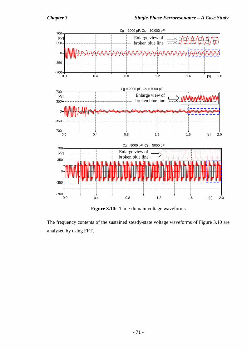
Chapter 3 Single-Phase Ferroresonance – A Case Study
- 71 -
Figure 3.10: Time-domain voltage waveforms
The frequency contents of the sustained steady-state voltage waveforms of Figure 3.10 are
analysed by using FFT,
0.0 0.4 0.8 1.2 1.6 2.0[s]-700
-350
0
350
700[kV]
Cg =1000 pF, Cs = 10,000 pF
Enlarge view of broken blue line
0.0 0.4 0.8 1.2 1.6 2.0[s]-700
-350
0
350
700[kV]
Cg = 2000 pF, Cs = 7000 pF
Enlarge view of broken blue line
0.0 0.4 0.8 1.2 1.6 2.0[s]-700
-350
0
350
700
[kV]
Cg = 8000 pF, Cs = 5000 pF
Enlarge view of broken blue line
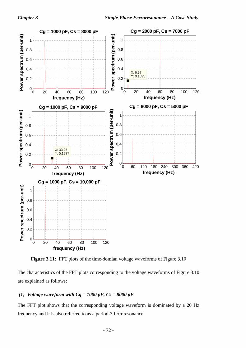
Chapter 3 Single-Phase Ferroresonance – A Case Study
- 72 -
Figure 3.11: FFT plots of the time-domian voltage waveforms of Figure 3.10
The characteristics of the FFT plots corresponding to the voltage waveforms of Figure 3.10
are explained as follows:
(1) Voltage waveform with Cg = 1000 pF, Cs = 8000 pF
The FFT plot shows that the corresponding voltage waveform is dominated by a 20 Hz
frequency and it is also referred to as a period-3 ferroresonance.
0 20 40 60 80 100 1200
0.2
0.4
0.6
0.8
1
Cg = 1000 pF, Cs = 8000 pF
frequency (Hz)
Pow
er s
pect
rum
(pe
r-un
it)
0 20 40 60 80 100 1200
0.2
0.4
0.6
0.8
1
Cg = 2000 pF, Cs = 7000 pF
frequency (Hz)
Pow
er s
pect
rum
(pe
r-un
it)
X: 6.67Y: 0.1595
0 20 40 60 80 100 1200
0.2
0.4
0.6
0.8
1
X: 33.25Y: 0.1287
Cg = 1000 pF, Cs = 9000 pF
frequency (Hz)
Pow
er s
pect
rum
(pe
r-un
it)
0 60 120 180 240 300 360 4200
0.2
0.4
0.6
0.8
1
Cg = 8000 pF, Cs = 5000 pF
frequency (Hz)
Pow
er s
pect
rum
(pe
r-un
it)
0 20 40 60 80 100 1200
0.2
0.4
0.6
0.8
1
Cg = 1000 pF, Cs = 10,000 pF
frequency (Hz)
Pow
er s
pect
rum
(pe
r-un
it)
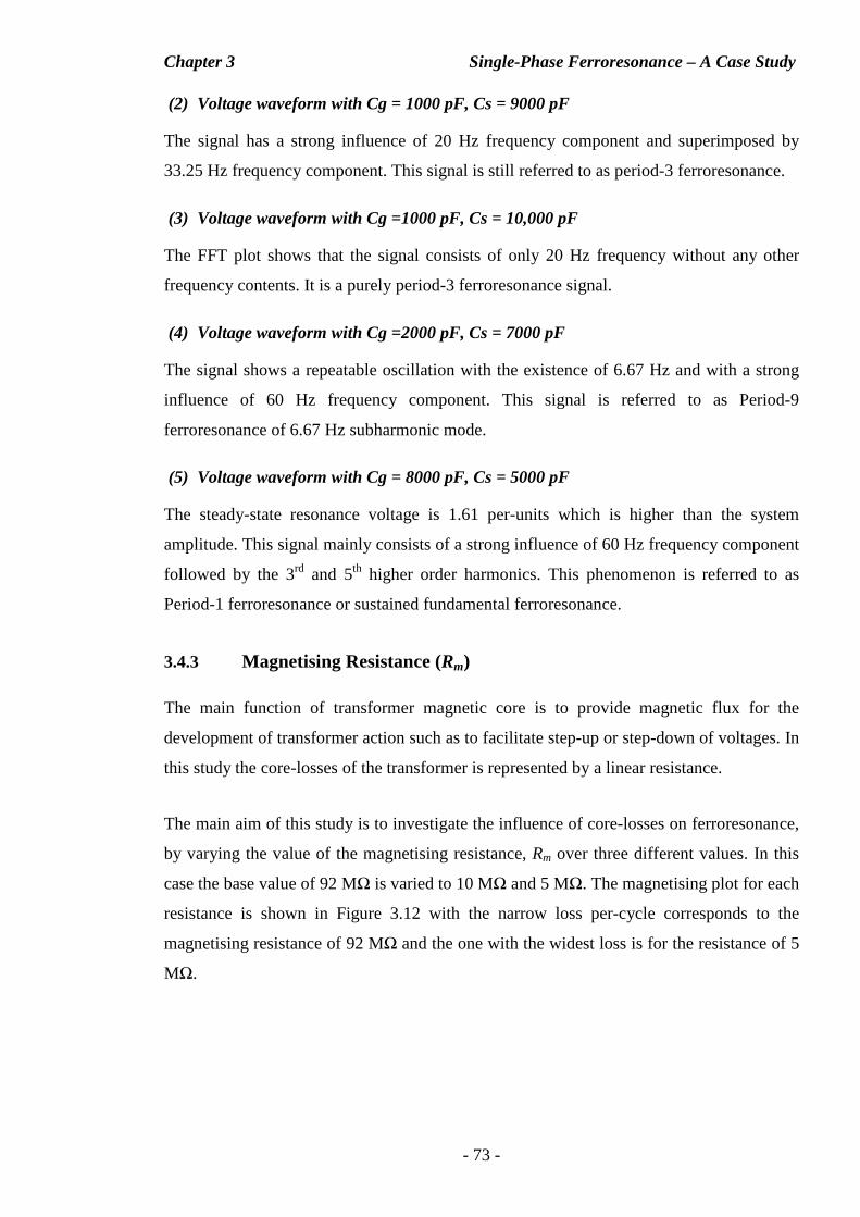
Chapter 3 Single-Phase Ferroresonance – A Case Study
- 73 -
(2) Voltage waveform with Cg = 1000 pF, Cs = 9000 pF
The signal has a strong influence of 20 Hz frequency component and superimposed by
33.25 Hz frequency component. This signal is still referred to as period-3 ferroresonance.
(3) Voltage waveform with Cg =1000 pF, Cs = 10,000 pF
The FFT plot shows that the signal consists of only 20 Hz frequency without any other
frequency contents. It is a purely period-3 ferroresonance signal.
(4) Voltage waveform with Cg =2000 pF, Cs = 7000 pF
The signal shows a repeatable oscillation with the existence of 6.67 Hz and with a strong
influence of 60 Hz frequency component. This signal is referred to as Period-9
ferroresonance of 6.67 Hz subharmonic mode.
(5) Voltage waveform with Cg = 8000 pF, Cs = 5000 pF
The steady-state resonance voltage is 1.61 per-units which is higher than the system
amplitude. This signal mainly consists of a strong influence of 60 Hz frequency component
followed by the 3rd and 5th higher order harmonics. This phenomenon is referred to as
Period-1 ferroresonance or sustained fundamental ferroresonance.
3.4.3 Magnetising Resistance (Rm)
The main function of transformer magnetic core is to provide magnetic flux for the
development of transformer action such as to facilitate step-up or step-down of voltages. In
this study the core-losses of the transformer is represented by a linear resistance.
The main aim of this study is to investigate the influence of core-losses on ferroresonance,
by varying the value of the magnetising resistance, Rm over three different values. In this
case the base value of 92 MΩ is varied to 10 MΩ and 5 MΩ. The magnetising plot for each
resistance is shown in Figure 3.12 with the narrow loss per-cycle corresponds to the
magnetising resistance of 92 MΩ and the one with the widest loss is for the resistance of 5
MΩ.
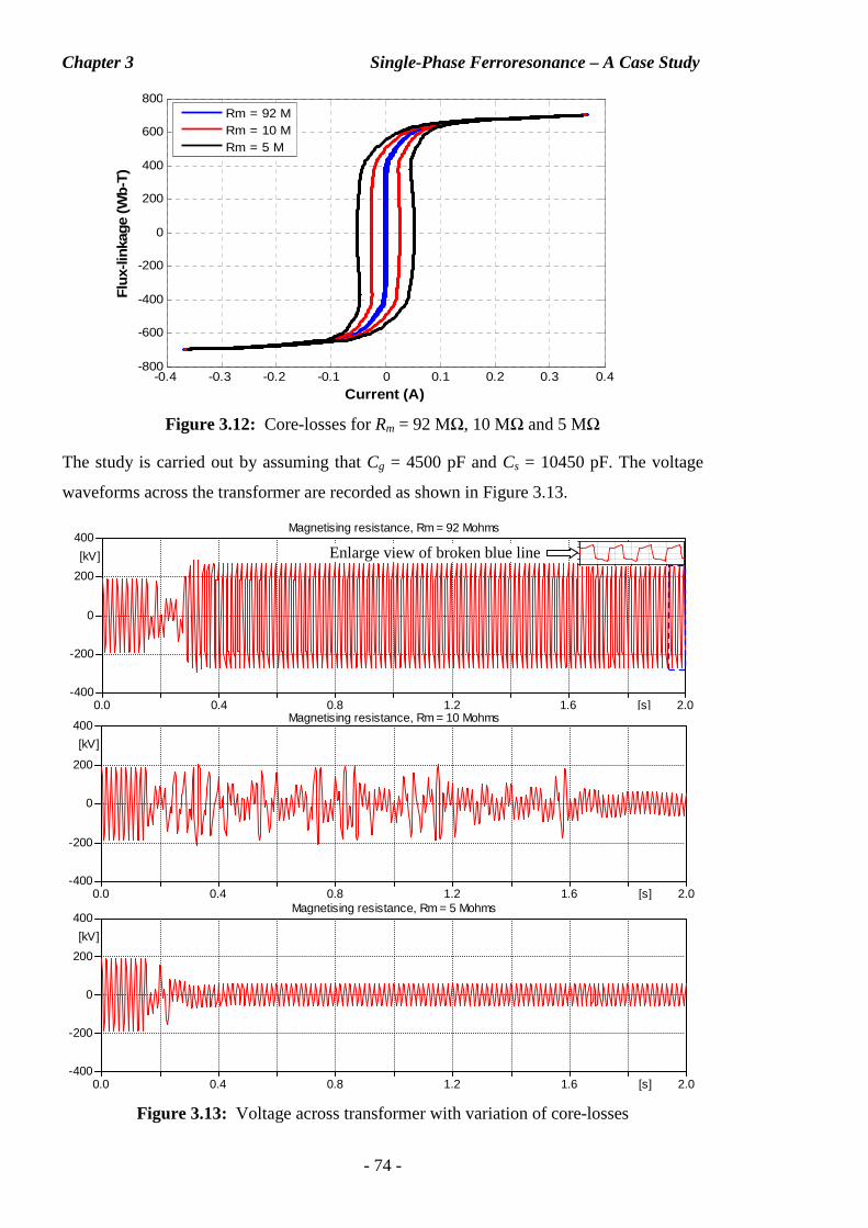
Chapter 3 Single-Phase Ferroresonance – A Case Study
- 74 -
Figure 3.12: Core-losses for Rm = 92 MΩ, 10 MΩ and 5 MΩ
The study is carried out by assuming that Cg = 4500 pF and Cs = 10450 pF. The voltage
waveforms across the transformer are recorded as shown in Figure 3.13.
Figure 3.13: Voltage across transformer with variation of core-losses
0.0 0.4 0.8 1.2 1.6 2.0[s]-400
-200
0
200
400
[kV]
Magnetising resistance, Rm = 92 Mohms
1.94 1.95 1.96 1.97 1.98 1.99 2.00[s]
[kV]
0.0 0.4 0.8 1.2 1.6 2.0[s]-400
-200
0
200
400
[kV]
Magnetising resistance, Rm = 10 Mohms
0.0 0.4 0.8 1.2 1.6 2.0[s]-400
-200
0
200
400
[kV]
Magnetising resistance, Rm = 5 Mohms
Enlarge view of broken blue line
-0.4 -0.3 -0.2 -0.1 0 0.1 0.2 0.3 0.4-800
-600
-400
-200
0
200
400
600
800
Current (A)
Flu
x-lin
kage
(W
b-T
)Rm = 92 MRm = 10 MRm = 5 M
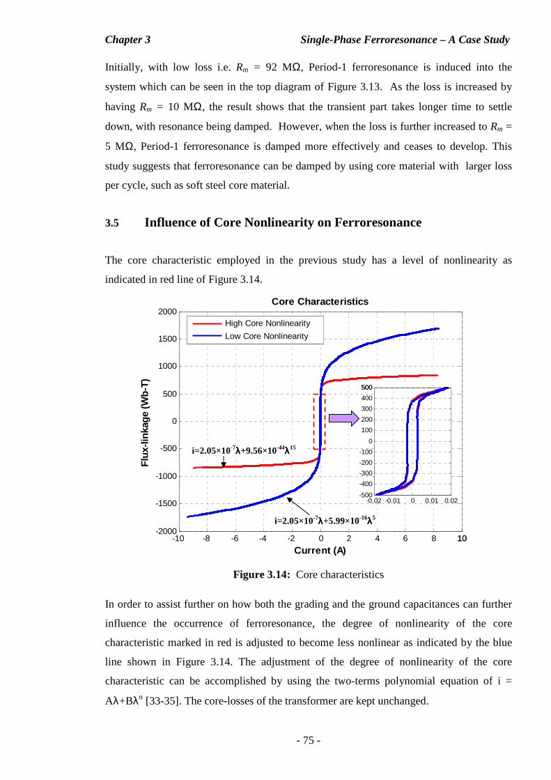
Chapter 3 Single-Phase Ferroresonance – A Case Study
- 75 -
Initially, with low loss i.e. Rm = 92 MΩ, Period-1 ferroresonance is induced into the
system which can be seen in the top diagram of Figure 3.13. As the loss is increased by
having Rm = 10 MΩ, the result shows that the transient part takes longer time to settle
down, with resonance being damped. However, when the loss is further increased to Rm =
5 MΩ, Period-1 ferroresonance is damped more effectively and ceases to develop. This
study suggests that ferroresonance can be damped by using core material with larger loss
per cycle, such as soft steel core material.
3.5 Influence of Core Nonlinearity on Ferroresonance
The core characteristic employed in the previous study has a level of nonlinearity as
indicated in red line of Figure 3.14.
Figure 3.14: Core characteristics
In order to assist further on how both the grading and the ground capacitances can further
influence the occurrence of ferroresonance, the degree of nonlinearity of the core
characteristic marked in red is adjusted to become less nonlinear as indicated by the blue
line shown in Figure 3.14. The adjustment of the degree of nonlinearity of the core
characteristic can be accomplished by using the two-terms polynomial equation of i =
Aλ+Bλn [33-35]. The core-losses of the transformer are kept unchanged.
-10 -8 -6 -4 -2 0 2 4 6 8 1010-2000
-1500
-1000
-500
0
500
1000
1500
2000Core Characteristics
Current (A)
Flu
x-lin
kage
(W
b-T
)
High Core Nonlinearity
Low Core Nonlinearity
-0.02 -0.01 0 0.01 0.02-500
-400
-300
-200
-100
0
100
200
300
400
500500
i=2.05×10⁻⁷λλλλ+9.56×10-44λλλλ15
i=2.05×10⁻⁷λλλλ+5.99×10⁻¹⁶λλλλ5
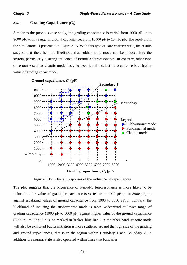
Chapter 3 Single-Phase Ferroresonance – A Case Study
- 76 -
3.5.1 Grading Capacitance (Cg)
Similar to the previous case study, the grading capacitance is varied from 1000 pF up to
8000 pF, with a range of ground capacitances from 10000 pF to 10,450 pF. The result from
the simulations is presented in Figure 3.15. With this type of core characteristic, the results
suggest that there is more likelihood that subharmonic mode can be induced into the
system, particularly a strong influence of Period-3 ferroresonance. In contrary, other type
of response such as chaotic mode has also been identified, but its occurrence is at higher
value of grading capacitance.
Figure 3.15: Overall responses of the influence of capacitances
The plot suggests that the occurrence of Period-1 ferroresonance is more likely to be
induced as the value of grading capacitance is varied from 1000 pF up to 8000 pF, up
against escalating values of ground capacitance from 1000 to 8000 pF. In contrary, the
likelihood of inducing the subharmonic mode is more widespread at lower range of
grading capacitance (1000 pF to 5000 pF) against higher value of the ground capacitance
(8000 pF to 10,450 pF), as marked in broken blue line. On the other hand, chaotic mode
will also be exhibited but its initiation is more scattered around the high side of the grading
and ground capacitances, that is in the region within Boundary 1 and Boundary 2. In
addition, the normal state is also operated within these two bundaries.
Legend: - Subharmonic mode - Fundamental mode - Chaotic mode
0
1000
1000 2000 3000 4000 5000 6000 7000 8000
Grading capacitance, Cg (pF)
Ground capacitance, Cs (pF)
2000
3000
4000
5000
6000
7000
8000
9000
10000
10450
Boundary 1
Boundary 2
Without Cs
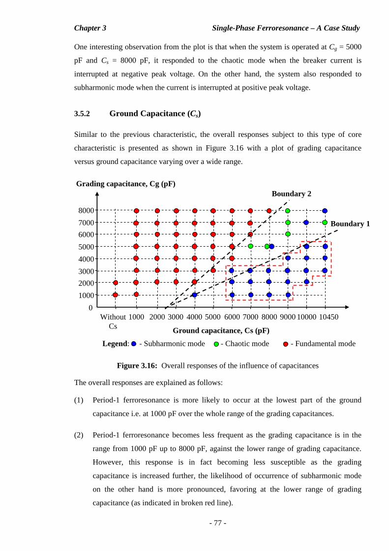
Chapter 3 Single-Phase Ferroresonance – A Case Study
- 77 -
One interesting observation from the plot is that when the system is operated at Cg = 5000
pF and Cs = 8000 pF, it responded to the chaotic mode when the breaker current is
interrupted at negative peak voltage. On the other hand, the system also responded to
subharmonic mode when the current is interrupted at positive peak voltage.
3.5.2 Ground Capacitance (Cs)
Similar to the previous characteristic, the overall responses subject to this type of core
characteristic is presented as shown in Figure 3.16 with a plot of grading capacitance
versus ground capacitance varying over a wide range.
Figure 3.16: Overall responses of the influence of capacitances
The overall responses are explained as follows:
(1) Period-1 ferroresonance is more likely to occur at the lowest part of the ground
capacitance i.e. at 1000 pF over the whole range of the grading capacitances.
(2) Period-1 ferroresonance becomes less frequent as the grading capacitance is in the
range from 1000 pF up to 8000 pF, against the lower range of grading capacitance.
However, this response is in fact becoming less susceptible as the grading
capacitance is increased further, the likelihood of occurrence of subharmonic mode
on the other hand is more pronounced, favoring at the lower range of grading
capacitance (as indicated in broken red line).
Legend: - Subharmonic mode - Chaotic mode - Fundamental mode
0
1000
2000
3000
4000
5000
6000
7000
8000
1000 2000 3000 4000 5000 6000 7000 8000 9000 10000 10450 Without Cs Ground capacitance, Cs (pF)
Grading capacitance, Cg (pF) Boundary 2
Boundary 1
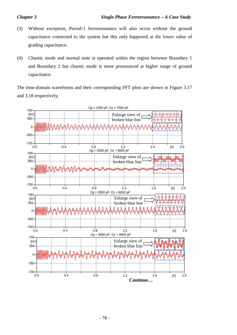
Chapter 3 Single-Phase Ferroresonance – A Case Study
- 78 -
(3) Without exception, Period-1 ferroresonance will also occur without the ground
capacitance connected to the system but this only happened at the lower value of
grading capacitance.
(4) Chaotic mode and normal state is operated within the region between Boundary 1
and Boundary 2 but chaotic mode is more pronounced at higher range of ground
capacitance.
The time-domain waveforms and their corresponding FFT plots are shown in Figure 3.17
and 3.18 respectively.
0.0 0.4 0.8 1.2 1.6 2.0[s]-700
-350
0
350
700[kV]
Cg = 1000 pF, Cs = 7000 pF
Enlarge view of broken blue line
0.0 0.4 0.8 1.2 1.6 2.0[s]-700
-350
0
350
700[kV]
Cg = 2000 pF, Cs = 9000 pF
Enlarge view of broken blue line
0.0 0.4 0.8 1.2 1.6 2.0[s]-700
-350
0
350
700[kV]
Cg = 3000 pF, Cs = 8000 pF
Enlarge view of broken blue line
Continue… 0.0 0.4 0.8 1.2 1.6 2.0[s]
-700
-350
0
350
700[kV]
Cg = 3000 pF, Cs = 9000 pF
Enlarge view of broken blue line
Continue…
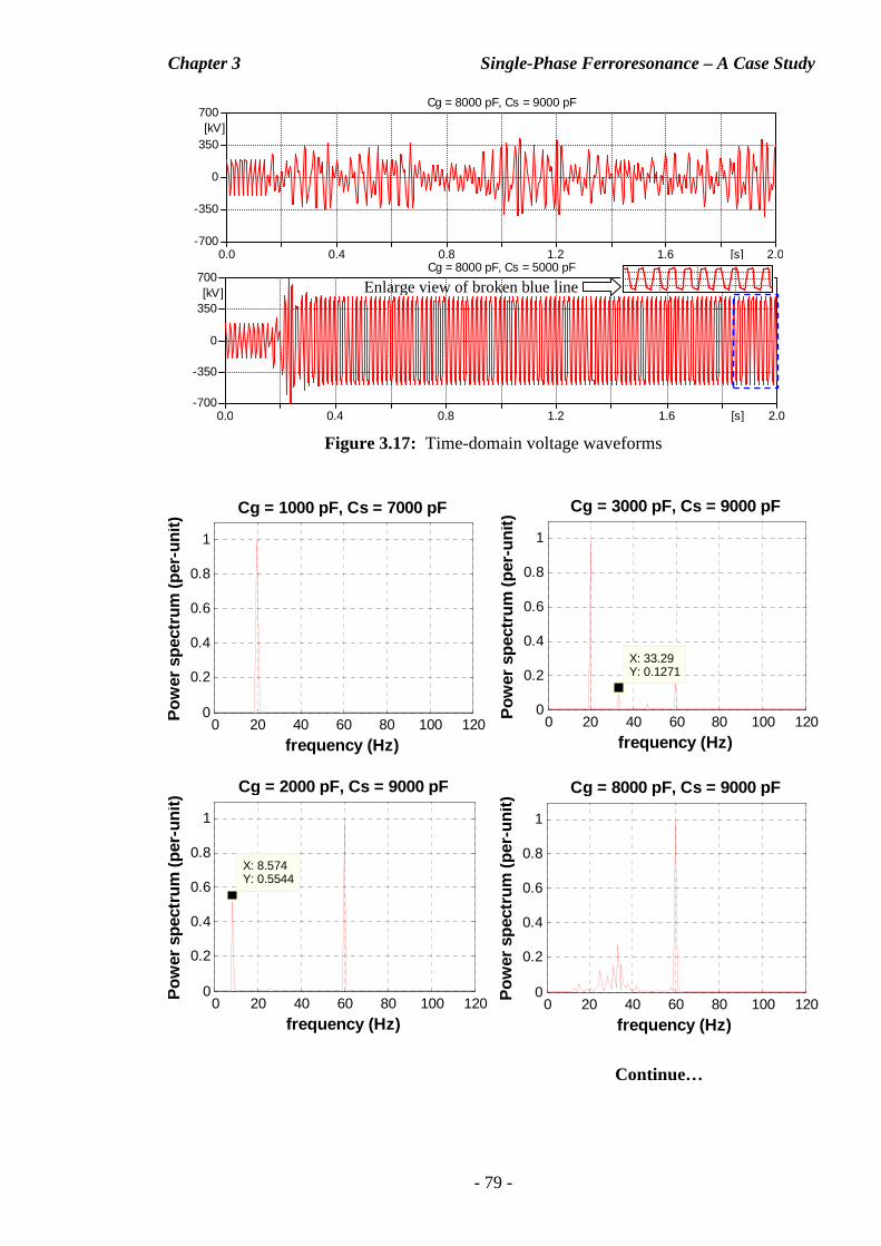
Chapter 3 Single-Phase Ferroresonance – A Case Study
- 79 -
Figure 3.17: Time-domain voltage waveforms
0.0 0.4 0.8 1.2 1.6 2.0[s]-700
-350
0
350
700[kV]
Cg = 8000 pF, Cs = 9000 pF
0.0 0.4 0.8 1.2 1.6 2.0[s]-700
-350
0
350
700[kV]
Cg = 8000 pF, Cs = 5000 pF
Enlarge view of broken blue line
0 20 40 60 80 100 1200
0.2
0.4
0.6
0.8
1
Cg = 1000 pF, Cs = 7000 pF
frequency (Hz)
Pow
er s
pect
rum
(pe
r-un
it)
0 20 40 60 80 100 1200
0.2
0.4
0.6
0.8
1
X: 33.29Y: 0.1271
Cg = 3000 pF, Cs = 9000 pF
frequency (Hz)
Pow
er s
pect
rum
(pe
r-un
it)
0 20 40 60 80 100 1200
0.2
0.4
0.6
0.8
1
Cg = 2000 pF, Cs = 9000 pF
frequency (Hz)
Pow
er s
pect
rum
(pe
r-un
it)
X: 8.574Y: 0.5544
0 20 40 60 80 100 1200
0.2
0.4
0.6
0.8
1
Cg = 8000 pF, Cs = 9000 pF
frequency (Hz)
Pow
er s
pect
rum
(pe
r-un
it)
Continue…
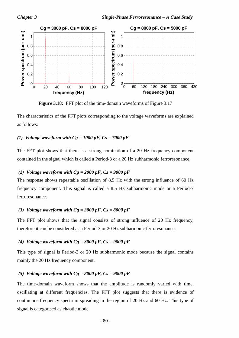
Chapter 3 Single-Phase Ferroresonance – A Case Study
- 80 -
Figure 3.18: FFT plot of the time-domain waveforms of Figure 3.17
The characteristics of the FFT plots corresponding to the voltage waveforms are explained
as follows:
(1) Voltage waveform with Cg = 1000 pF, Cs = 7000 pF
The FFT plot shows that there is a strong nomination of a 20 Hz frequency component
contained in the signal which is called a Period-3 or a 20 Hz subharmonic ferroresonance.
(2) Voltage waveform with Cg = 2000 pF, Cs = 9000 pF
The response shows repeatable oscillation of 8.5 Hz with the strong influence of 60 Hz
frequency component. This signal is called a 8.5 Hz subharmonic mode or a Period-7
ferroresonance.
(3) Voltage waveform with Cg = 3000 pF, Cs = 8000 pF
The FFT plot shows that the signal consists of strong influence of 20 Hz frequency,
therefore it can be considered as a Period-3 or 20 Hz subharmonic ferroresonance.
(4) Voltage waveform with Cg = 3000 pF, Cs = 9000 pF
This type of signal is Period-3 or 20 Hz subharmonic mode because the signal contains
mainly the 20 Hz frequency component.
(5) Voltage waveform with Cg = 8000 pF, Cs = 9000 pF
The time-domain waveform shows that the amplitude is randomly varied with time,
oscillating at different frequencies. The FFT plot suggests that there is evidence of
continuous frequency spectrum spreading in the region of 20 Hz and 60 Hz. This type of
signal is categorised as chaotic mode.
0 20 40 60 80 100 1200
0.2
0.4
0.6
0.8
1
Cg = 3000 pF, Cs = 8000 pF
frequency (Hz)
Pow
er s
pect
rum
(pe
r-un
it)
0 60 120 180 240 300 360 4204200
0.2
0.4
0.6
0.8
1
Cg = 8000 pF, Cs = 5000 pF
frequency (Hz)
Pow
er s
pect
rum
(pe
r-un
it)
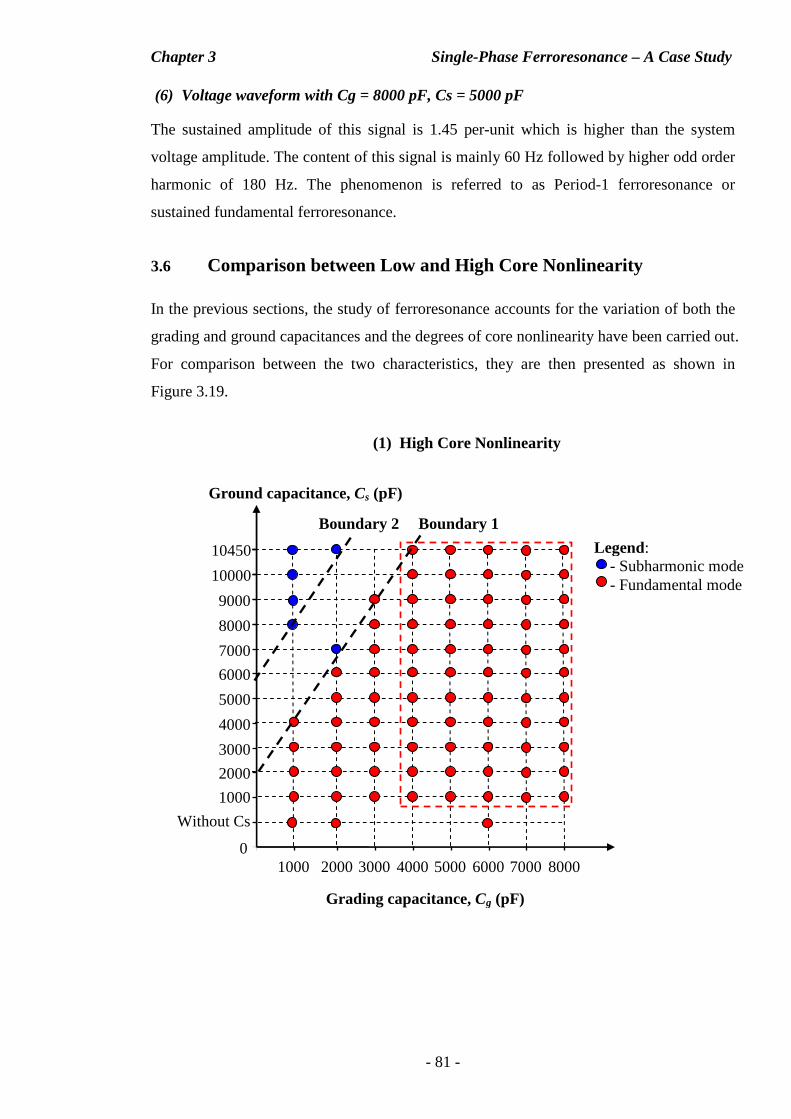
Chapter 3 Single-Phase Ferroresonance – A Case Study
- 81 -
(6) Voltage waveform with Cg = 8000 pF, Cs = 5000 pF
The sustained amplitude of this signal is 1.45 per-unit which is higher than the system
voltage amplitude. The content of this signal is mainly 60 Hz followed by higher odd order
harmonic of 180 Hz. The phenomenon is referred to as Period-1 ferroresonance or
sustained fundamental ferroresonance.
3.6 Comparison between Low and High Core Nonlinearity
In the previous sections, the study of ferroresonance accounts for the variation of both the
grading and ground capacitances and the degrees of core nonlinearity have been carried out.
For comparison between the two characteristics, they are then presented as shown in
Figure 3.19.
(1) High Core Nonlinearity
Grading capacitance, Cg (pF)
Legend: - Subharmonic mode - Fundamental mode
0
1000
1000 2000 3000 4000 5000 6000 7000 8000
Ground capacitance, Cs (pF)
2000
3000
4000
5000
6000
7000
8000
9000
10000
10450
Boundary 1 Boundary 2
Without Cs
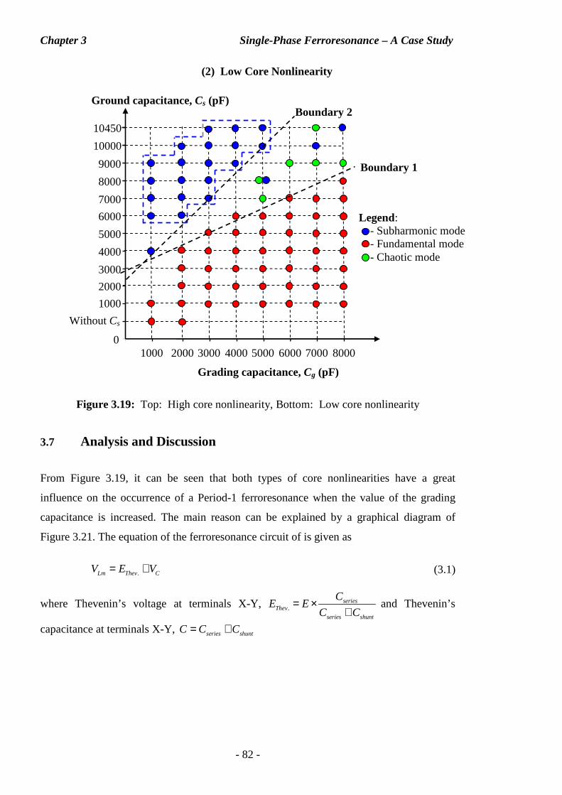
Chapter 3 Single-Phase Ferroresonance – A Case Study
- 82 -
Figure 3.19: Top: High core nonlinearity, Bottom: Low core nonlinearity
3.7 Analysis and Discussion
From Figure 3.19, it can be seen that both types of core nonlinearities have a great
influence on the occurrence of a Period-1 ferroresonance when the value of the grading
capacitance is increased. The main reason can be explained by a graphical diagram of
Figure 3.21. The equation of the ferroresonance circuit of is given as
.Lm Thev CV E V= + (3.1)
where Thevenin’s voltage at terminals X-Y, .series
Thev
series shunt
CE E
C C= ×
+and Thevenin’s
capacitance at terminals X-Y, series shuntC C C= +
(2) Low Core Nonlinearity
Legend: - Subharmonic mode - Fundamental mode - Chaotic mode
0
1000
1000 2000 3000 4000 5000 6000 7000 8000
Grading capacitance, Cg (pF)
Ground capacitance, Cs (pF)
2000
3000
4000
5000
6000
7000
8000
9000
10000
10450
Boundary 1
Boundary 2
Without Cs
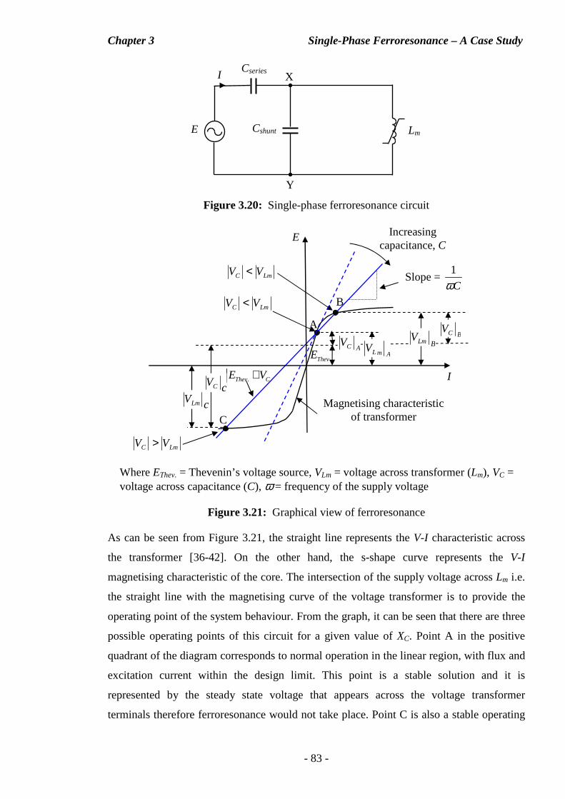
Chapter 3 Single-Phase Ferroresonance – A Case Study
- 83 -
Figure 3.20: Single-phase ferroresonance circuit
Figure 3.21: Graphical view of ferroresonance
As can be seen from Figure 3.21, the straight line represents the V-I characteristic across
the transformer [36-42]. On the other hand, the s-shape curve represents the V-I
magnetising characteristic of the core. The intersection of the supply voltage across Lm i.e.
the straight line with the magnetising curve of the voltage transformer is to provide the
operating point of the system behaviour. From the graph, it can be seen that there are three
possible operating points of this circuit for a given value of XC. Point A in the positive
quadrant of the diagram corresponds to normal operation in the linear region, with flux and
excitation current within the design limit. This point is a stable solution and it is
represented by the steady state voltage that appears across the voltage transformer
terminals therefore ferroresonance would not take place. Point C is also a stable operating
Increasing capacitance, C
E
I
A
B
C
.ThevE
.Thev CE V+
AmLV
Magnetising characteristic of transformer
cVC
cVLm
BLmV
LmC VV >
LmC VV <
LmC VV <
ACVBCV
Slope = 1
Cω
Where EThev. = Thevenin’s voltage source, VLm = voltage across transformer (Lm), VC = voltage across capacitance (C), ω = frequency of the supply voltage
E
Cseries
Cshunt
I
Lm
X
Y
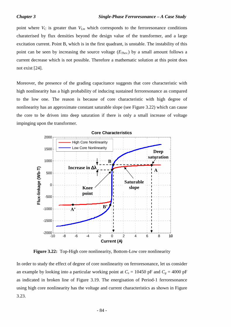
Chapter 3 Single-Phase Ferroresonance – A Case Study
- 84 -
point where VC is greater than VLm which corresponds to the ferroresonance conditions
charaterised by flux densities beyond the design value of the transformer, and a large
excitation current. Point B, which is in the first quadrant, is unstable. The instability of this
point can be seen by increasing the source voltage (EThev.) by a small amount follows a
current decrease which is not possible. Therefore a mathematic solution at this point does
not exist [24].
Moreover, the presence of the grading capacitance suggests that core characteristic with
high nonlinearity has a high probability of inducing sustained ferroresonance as compared
to the low one. The reason is because of core characteristic with high degree of
nonlinearity has an approximate constant saturable slope (see Figure 3.22) which can cause
the core to be driven into deep saturation if there is only a small increase of voltage
impinging upon the transformer.
Figure 3.22: Top-High core nonlinearity, Bottom-Low core nonlinearity
In order to study the effect of degree of core nonlinearity on ferroresonance, let us consider
an example by looking into a particular working point at Cs = 10450 pF and Cg = 4000 pF
as indicated in broken line of Figure 3.19. The energisation of Period-1 ferroresonance
using high core nonlinearity has the voltage and current characteristics as shown in Figure
3.23.
-10 -8 -6 -4 -2 0 2 4 6 8 1010-2000
-1500
-1000
-500
0
500
1000
1500
2000Core Characteristics
Current (A)
Flu
x-lin
kage
(Wb-
T)
High Core Nonlinearity
Low Core Nonlinearity
Increase in ∆∆∆∆λλλλ
Saturable slope
Deep saturation
Knee point
B
A
A’ B’
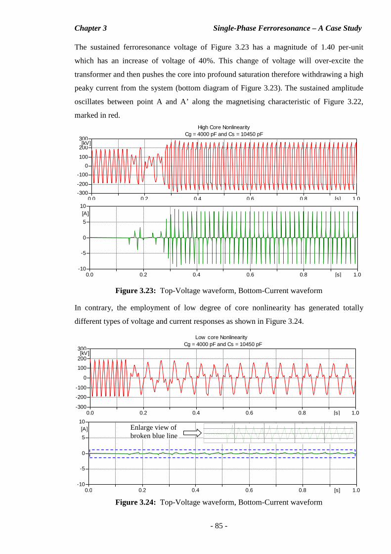
Chapter 3 Single-Phase Ferroresonance – A Case Study
- 85 -
The sustained ferroresonance voltage of Figure 3.23 has a magnitude of 1.40 per-unit
which has an increase of voltage of 40%. This change of voltage will over-excite the
transformer and then pushes the core into profound saturation therefore withdrawing a high
peaky current from the system (bottom diagram of Figure 3.23). The sustained amplitude
oscillates between point A and A’ along the magnetising characteristic of Figure 3.22,
marked in red.
Figure 3.23: Top-Voltage waveform, Bottom-Current waveform
In contrary, the employment of low degree of core nonlinearity has generated totally
different types of voltage and current responses as shown in Figure 3.24.
Figure 3.24: Top-Voltage waveform, Bottom-Current waveform
0.0 0.2 0.4 0.6 0.8 1.0[s]-300
-200
-100
0
100
200
300[kV]
High Core NonlinearityCg = 4000 pF and Cs = 10450 pF
0.0 0.2 0.4 0.6 0.8 1.0[s]-10
-5
0
5
10[A]
0.0 0.2 0.4 0.6 0.8 1.0[s]-300
-200
-100
0
100
200
300[kV]
Low core Nonlinearity Cg = 4000 pF and Cs = 10450 pF
0.0 0.2 0.4 0.6 0.8 1.0[s]-10
-5
0
5
10[A] Enlarge view of
broken blue line
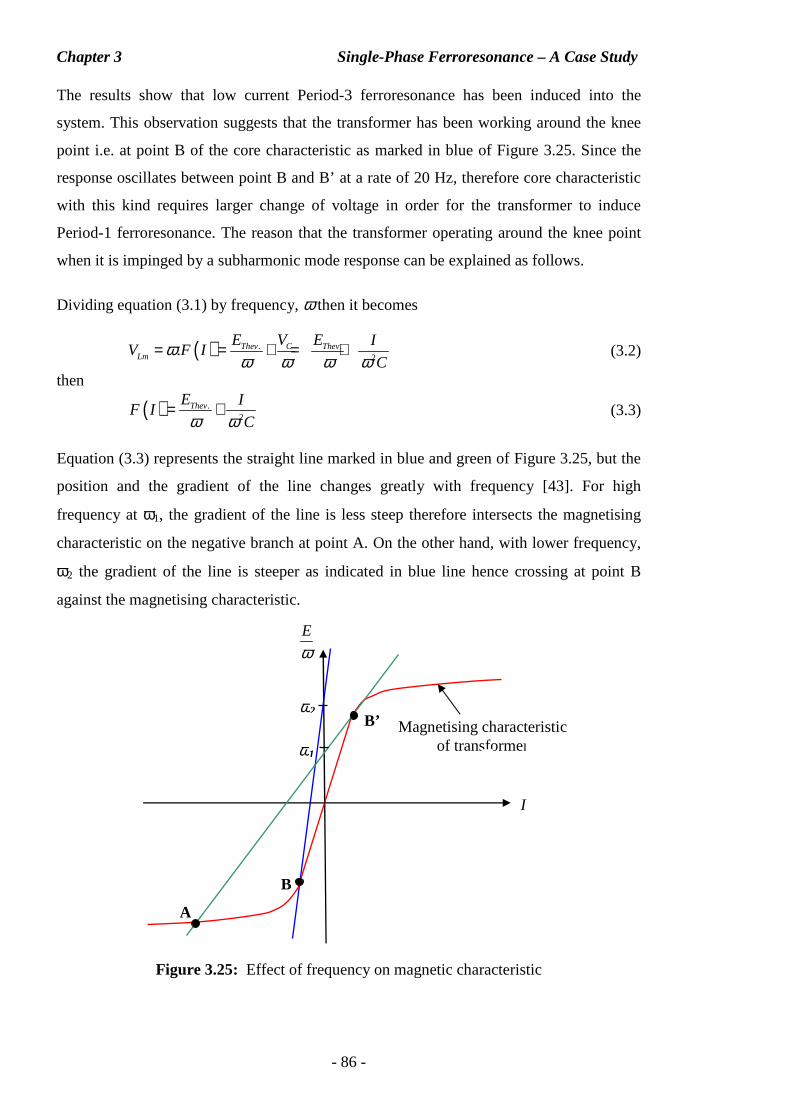
Chapter 3 Single-Phase Ferroresonance – A Case Study
- 86 -
The results show that low current Period-3 ferroresonance has been induced into the
system. This observation suggests that the transformer has been working around the knee
point i.e. at point B of the core characteristic as marked in blue of Figure 3.25. Since the
response oscillates between point B and B’ at a rate of 20 Hz, therefore core characteristic
with this kind requires larger change of voltage in order for the transformer to induce
Period-1 ferroresonance. The reason that the transformer operating around the knee point
when it is impinged by a subharmonic mode response can be explained as follows.
Dividing equation (3.1) by frequency, ω then it becomes
( ) . .2
. Thev C ThevLm
E V E IV F I
Cω
ω ω ω ω= = + = + (3.2)
then
( ) .2
ThevE IF I
Cω ω= + (3.3)
Equation (3.3) represents the straight line marked in blue and green of Figure 3.25, but the
position and the gradient of the line changes greatly with frequency [43]. For high
frequency at ω1, the gradient of the line is less steep therefore intersects the magnetising
characteristic on the negative branch at point A. On the other hand, with lower frequency,
ω2 the gradient of the line is steeper as indicated in blue line hence crossing at point B
against the magnetising characteristic.
Figure 3.25: Effect of frequency on magnetic characteristic
I
B
Magnetising characteristic of transformer
E
ω
A
ω2
ω1
B’
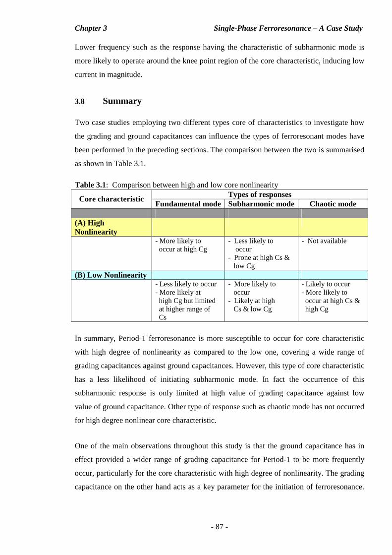
Chapter 3 Single-Phase Ferroresonance – A Case Study
- 87 -
Lower frequency such as the response having the characteristic of subharmonic mode is
more likely to operate around the knee point region of the core characteristic, inducing low
current in magnitude.
3.8 Summary
Two case studies employing two different types core of characteristics to investigate how
the grading and ground capacitances can influence the types of ferroresonant modes have
been performed in the preceding sections. The comparison between the two is summarised
as shown in Table 3.1.
Table 3.1: Comparison between high and low core nonlinearity Types of responses Core characteristic
Fundamental mode Subharmonic mode Chaotic mode (A) High Nonlinearity
- More likely to occur at high Cg
- Less likely to occur - Prone at high Cs & low Cg
- Not available
(B) Low Nonlinearity - Less likely to occur
- More likely at high Cg but limited at higher range of Cs
- More likely to occur - Likely at high Cs & low Cg
- Likely to occur - More likely to occur at high Cs & high Cg
In summary, Period-1 ferroresonance is more susceptible to occur for core characteristic
with high degree of nonlinearity as compared to the low one, covering a wide range of
grading capacitances against ground capacitances. However, this type of core characteristic
has a less likelihood of initiating subharmonic mode. In fact the occurrence of this
subharmonic response is only limited at high value of grading capacitance against low
value of ground capacitance. Other type of response such as chaotic mode has not occurred
for high degree nonlinear core characteristic.
One of the main observations throughout this study is that the ground capacitance has in
effect provided a wider range of grading capacitance for Period-1 to be more frequently
occur, particularly for the core characteristic with high degree of nonlinearity. The grading
capacitance on the other hand acts as a key parameter for the initiation of ferroresonance.

Chapter 3 Single-Phase Ferroresonance – A Case Study
- 88 -
This is because Period-1 response is still able to be induced without the presence of the
ground capacitance.
In contrast, core characteristic employing low degree of nonlinearity has a less chance for
the Period-1 ferroresonance to occur. Instead this type of response occurs in a confined
range of high ground capacitance against high value of grading capacitance. Subsequently,
it is more pronounced for subharmonic mode to be induced, confining at high ground
capacitance and low value of grading capacitances. Furthermore, chaotic mode can also be
exhibited but restricted around high ground and grading capacitances.
The overall study from the above can thus provide an overall glimpse on how a system
network responds to ferroresonance for the variation of the following parameters; the
grading capacitance, the ground capacitance, the core-losses and the use of different degree
of nonlinearity of core characteristics.
Chapter 4 System Component Models for Ferroresonance
- 89 -
CHAPTER 4 CHAPTER 4 CHAPTER 4 CHAPTER 4
444... SSSYYYSSSTTTEEEMMM CCCOOOMMM PPPOOONNNEEENNNTTT MMM OOODDDEEELLL SSS FFFOOORRR FFFEEERRRRRROOORRREEESSSOOONNNAAANNNCCCEEE
4.1 Introduction
In the preceding chapter, the study of a single-phase ferroresonance circuit has been carried
out to investigate the fundamental behaviours of the phenomenon when the parameters are
varied.
One of the main aims of this thesis is to determine the best possible predefined models in
ATPDraw so that each of the components can be suitably represented for modeling the real
case circuit which has experienced ferroresonance. It is therefore the objective of this
chapter to firstly introduce the technical aspects of the power system components, and to
identify the best possible model for the study of ferroresonance that are available in
ATPDraw. As ferroresonance is classified as a low frequency transient, much attention is
then concentrated on the circuit breaker, the transmission line and the power transformer
which are concerned. The criteria to be used for determining the suitability of each of the
predefined models are taken in relation to the modeling guidance proposed by CIGRE and
are explained accordingly.
4.2 400-kV Circuit Breaker
A circuit breaker is a mechanical switching device, regardless of its location in the power
system network, it is required for controlling purposes by switching a circuit in, by
carrying load currents and by switching a circuit off under manual or automatic
supervision. In its simplistic term, the main function of the circuit breaker is to act as a
switch capable of making, carrying, and breaking currents under the normal and abnormal
conditions.
There are five basic types of switch models [44] available in ATPDraw namely: the time-
controlled switch, the gap switch, diode switch, the thyristor switch and the measuring
switch. The only one relevant to the circuit breaker is the time-controlled switch which is
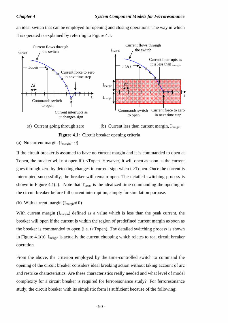
Chapter 4 System Component Models for Ferroresonance
- 90 -
an ideal switch that can be employed for opening and closing operations. The way in which
it is operated is explained by referring to Figure 4.1.
(a) Current going through zero (b) Current less than current margin, Imargin
Figure 4.1: Circuit breaker opening criteria
(a) No current margin (Imargin= 0)
If the circuit breaker is assumed to have no current margin and it is commanded to open at
Topen, the breaker will not open if t <Topen. However, it will open as soon as the current
goes through zero by detecting changes in current sign when t >Topen. Once the current is
interrupted successfully, the breaker will remain open. The detailed switching process is
shown in Figure 4.1(a). Note that Topen is the idealized time commanding the opening of
the circuit breaker before full current interruption, simply for simulation purpose.
(b) With current margin (Imargin≠ 0)
With current margin (Imargin) defined as a value which is less than the peak current, the
breaker will open if the current is within the region of predefined current margin as soon as
the breaker is commanded to open (i.e. t>Topen). The detailed switching process is shown
in Figure 4.1(b). Imargin is actually the current chopping which relates to real circuit breaker
operation.
From the above, the criterion employed by the time-controlled switch to command the
opening of the circuit breaker considers ideal breaking action without taking account of arc
and restrike characteristics. Are these characteristics really needed and what level of model
complexity for a circuit breaker is required for ferroresonance study? For ferroresonance
study, the circuit breaker with its simplistic form is sufficient because of the following:
Current flows through the switch
∆t
t
iswitch
Current interrupts as it changes sign
Commands switch to open
Current force to zero in next time step
Topen
Current flows through the switch
∆t
t
iswitch
Current interrupts as it is less than Imargin
Commands switch to open
Imargin
Imargin
Current force to zero in next time step
i (A)
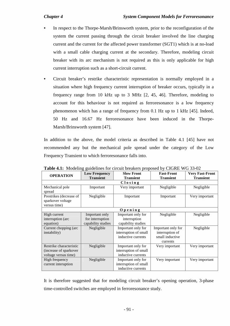
Chapter 4 System Component Models for Ferroresonance
- 91 -
• In respect to the Thorpe-Marsh/Brinsworth system, prior to the reconfiguration of the
system the current passing through the circuit breaker involved the line charging
current and the current for the affected power transformer (SGT1) which is at no-load
with a small cable charging current at the secondary. Therefore, modeling circuit
breaker with its arc mechanism is not required as this is only applicable for high
current interruption such as a short-circuit current.
• Circuit breaker’s restrike characteristic representation is normally employed in a
situation where high frequency current interruption of breaker occurs, typically in a
frequency range from 10 kHz up to 3 MHz [2, 45, 46]. Therefore, modeling to
account for this behaviour is not required as ferroresonance is a low frequency
phenomenon which has a range of frequency from 0.1 Hz up to 1 kHz [45]. Indeed,
50 Hz and 16.67 Hz ferroresonance have been induced in the Thorpe-
Marsh/Brinsworth system [47].
In addition to the above, the model criteria as described in Table 4.1 [45] have not
recommended any but the mechanical pole spread under the category of the Low
Frequency Transient to which ferroresonance falls into.
Table 4.1: Modeling guidelines for circuit breakers proposed by CIGRE WG 33-02
OPERATION Low Frequency
Transient Slow Front Transient
Fast-Front Transient
Very Fast-Front Transient
C l o s i n g Mechanical pole spread
Important Very important Negligible Negligible
Prestrikes (decrease of sparkover voltage versus time)
Negligible Important Important Very important
O p e n i n g High current interruption (arc equation)
Important only for interruption
capability studies
Important only for interruption
capability studies
Negligible Negligible
Current chopping (arc instability)
Negligible Important only for interruption of small inductive currents
Important only for interruption of small inductive
currents
Negligible
Restrike characteristic (increase of sparkover voltage versus time)
Negligible Important only for interruption of small inductive currents
Very important Very important
High frequency current interuption
Negligible Important only for interruption of small inductive currents
Very important Very important
It is therefore suggested that for modeling circuit breaker’s opening operation, 3-phase
time-controlled switches are employed in ferroresonance study.
Chapter 4 System Component Models for Ferroresonance
- 92 -
4.3 Power Transformer
Electrical power produced from generation stations has to be delivered over a long distance
for consumption. To enable a large amount of power to be transmitted through small
conductors while keeping the losses small the use of very high transmission voltages is
required. Therefore, a step-up transformer is employed to increase the voltage to a very
high level. In the distribution level, the high voltages are then step-down for distribution to
customers.
Transformers are considered to be one of the most universal components employed in
power transmission and distribution networks. Their complex structures mainly consist of
electromagnetic circuits. They are operating in a linear region of their magnetic
characteristic, drawing transformation of steady state sinusoidal voltages and currents.
However, there are instances the operating linear region is breached when the transformer
is subjected to the influence of an abnormal event. This incident could eventually lead to
one of the low frequency transient events, a phenomenon known as ferroresonance.
High peaky current will be drawn from the system once transformers are impinged upon by
ferroresonance. In view of this, transformers are constrained in their performance by the
magnetic flux limitations of the core. Core materials cannot support infinite magnetic flux
densities: they tend to “saturate” at a certain level, meaning that further increases in
magnetic field force (m.m.f) do not result in proportional increases in magnetic field flux
(Φ). In this regard, the transformer cores become nonlinear and they have to be modeled
correctly to characterise saturation effect. Saturation effect introduces distortion of the
excitation current when the cores are under the influence of nonlinearity.
In modeling the nonlinear core of transformer, core saturation effect can be represented by
either a single-value curve alone or with loss to account for major hysteresis curve. Both
representations are studied to differentiate their variations in generating the excitation
currents. In addition, the harmonic contents of the excitation currents operating along the
core characteristic are also studied.
Two mathematical approaches based on [35, 48, 49] are used to characteristic core
saturation; they are the single-value curve (without loss) and the major hysteresis curve
(with loss), and each of them is presented in the following section.
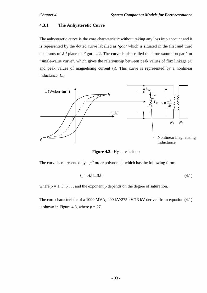
Chapter 4 System Component Models for Ferroresonance
- 93 -
4.3.1 The Anhysteretic Curve
The anhysteretic curve is the core characteristic without taking any loss into account and it
is represented by the dotted curve labelled as ‘gob’ which is situated in the first and third
quadrants of λ-i plane of Figure 4.2. The curve is also called the “true saturation part” or
“single-value curve”, which gives the relationship between peak values of flux linkage (λ)
and peak values of magnetising current (i). This curve is represented by a nonlinear
inductance, Lm.
Figure 4.2: Hysteresis loop
The curve is represented by a pth order polynomial which has the following form:
p
mi A Bλ λ= + (4.1) where p = 1, 3, 5 . . . and the exponent p depends on the degree of saturation.
The core characteristic of a 1000 MVA, 400 kV/275 kV/13 kV derived from equation (4.1)
is shown in Figure 4.3, where p = 27.
λ (Weber-turn) b
o
g
Lm
N1 N2
iexc
Nonlinear magnetising inductance
im
dt
dv
λ=
i (A)
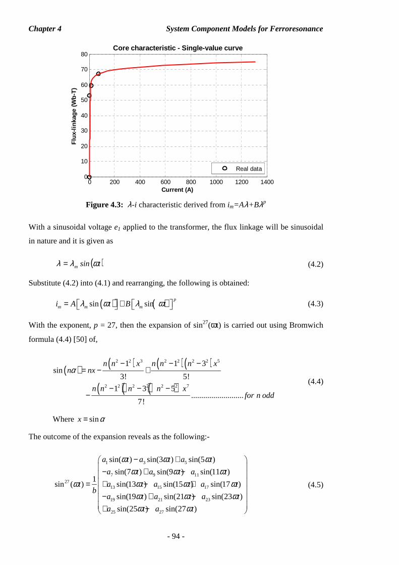
Chapter 4 System Component Models for Ferroresonance
- 94 -
Figure 4.3: λ-i characteristic derived from im=Aλ+Bλp
With a sinusoidal voltage e1 applied to the transformer, the flux linkage will be sinusoidal
in nature and it is given as
( )tsinm ωλλ = (4.2)
Substitute (4.2) into (4.1) and rearranging, the following is obtained:
( ) ( )sin sinp
m m mi A t B tλ ω λ ω= + (4.3)
With the exponent, p = 27, then the expansion of sin27(ωt) is carried out using Bromwich
formula (4.4) [50] of,
( ) ( ) ( ) ( )
( )( ) ( )
2 2 3 2 2 2 2 5
2 2 2 2 2 2 7
1 1 3sin
3! 5!
1 3 5..........................
7!
n n x n n n xn nx
n n n n xfor n odd
α− − −
= − +
− − −−
(4.4)
Where sinx α=
The outcome of the expansion reveals as the following:-
1 3 5
7 9 11
2713 15 17
19 21 23
25 27
sin( ) sin(3 ) sin(5 )
sin(7 ) sin(9 ) sin(11 )1
sin ( ) sin(13 ) sin(15 ) sin(17 )
sin(19 ) sin(21 ) sin(23 )
sin(25 ) sin(27 )
a t a t a t
a t a t a t
t a t a t a tb
a t a t a t
a t a t
ω ω ωω ω ω
ω ω ω ωω ω ωω ω
− + − + − = + − +
− + − + −
(4.5)
0 200 400 600 800 1000 1200 14000
10
20
30
40
50
60
70
80Core characteristic - Single-value curve
Current (A)
Flu
x-lin
kage
(W
b-T
)
Real data
Chapter 4 System Component Models for Ferroresonance
- 95 -
where the constants are found to be:
b = 67108864; a1 = 20058300; a3 = 17383860; a5 = 13037895; a7 = 8436285; a9 = 4686825;
a11 = 2220075; a13 = 888030; a15 = 296010; a17 = 80730; a19 = 17550; a21 = 2925; a23 = 351;
a25 = 27; a27 = 1;
Substituting (4.5) into (4.3)
( )
1 3 5
7 9 11
13 15 17
19 21 23
25 27
sin( ) sin(3 ) sin(5 )
sin(7 ) sin(9 ) sin(11 )1
'sin ' sin(13 ) sin(15 ) sin(17 )
sin(19 ) sin(21 ) sin(23 )
sin(25 ) sin(27 )
m
a t a t a t
a t a t a t
i A t B a t a t a tb
a t a t a t
a t a t
ω ω ωω ω ω
ω ω ω ωω ω ωω ω
− + − + − = + + − +
− + − + −
(4.6)
Where ' mA Aλ= , 27' mB Bλ=
Finally, the general equation of magnetising current in the time domain without the
hysteresis effect is derived as,
( ) ( )1 3 5 7 9
11 13 15 17
19 21 23 25 27
ˆ ˆ ˆ ˆ ˆsin sin 3 sin(5 ) sin(7 ) sin(9 )
ˆ ˆ ˆsin(11 ) sin(13 ) sin(15 ) sin(17 )
ˆ ˆ ˆ ˆ ˆsin(19 ) sin(21 ) sin(23 ) sin(25 ) sin(27 )
mi I t I t I t I t I t
I t I t I t a t
I t I t I t I t I t
ω ω ω ω ω
ω ω ω ω
ω ω ω ω ω
= + + + +
+ + + +
+ + + + +
(4.7)
Where
11 ' '
aI A B
b= + , 3
3 'a
I Bb
= − , 55 '
aI B
b= , 7
7 'a
I Bb
= − , 99 '
aI B
b= , 11
11ˆ '
aI B
b= − ,
1313ˆ '
aI B
b= , 15
15ˆ '
aI B
b= − , 17
17ˆ '
aI B
b= , 19
19ˆ '
aI B
b= − , 21
21ˆ '
aI B
b= ,
2323ˆ '
aI B
b= − , '25
25ˆ aI B
b= , '27
27ˆ aI B
b= −
The magnetising current, im together with its harmonic contents up to 27th can be plotted
using MATLAB. The magnetising currents, im operating along the core λ-i characteristic
labeled as A, B, C, D and E of Figure 4.4 are studied.
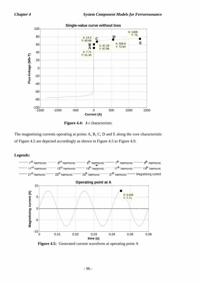
Chapter 4 System Component Models for Ferroresonance
- 96 -
Figure 4.4: λ-i characteristic
The magnetising currents operating at points A, B, C, D and E along the core characteristic
of Figure 4.5 are depicted accordingly as shown in Figure 4.5 to Figure 4.9.
Figure 4.5: Generated current waveform at operating point A
Legends:
-1500 -1000 -500 0 500 1000 1500-100
-80
-60
-40
-20
0
20
40
60
80
100
X: 7.71Y: 51.34
X: 13.3Y: 60.68
X: 97.29Y: 67.86
X: 558.8Y: 72.64
Single-value curve without loss
Current (A)
Flu
x-lin
kage
(W
b-T
)X: 1308
Y: 75
A B
C D
E
0 0.01 0.02 0.03 0.04 0.05 0.06-10
-5
0
5
10Operating point at A
time (s)
Mag
netis
ing
curr
ent (
A) X: 0.045
Y: 7.71
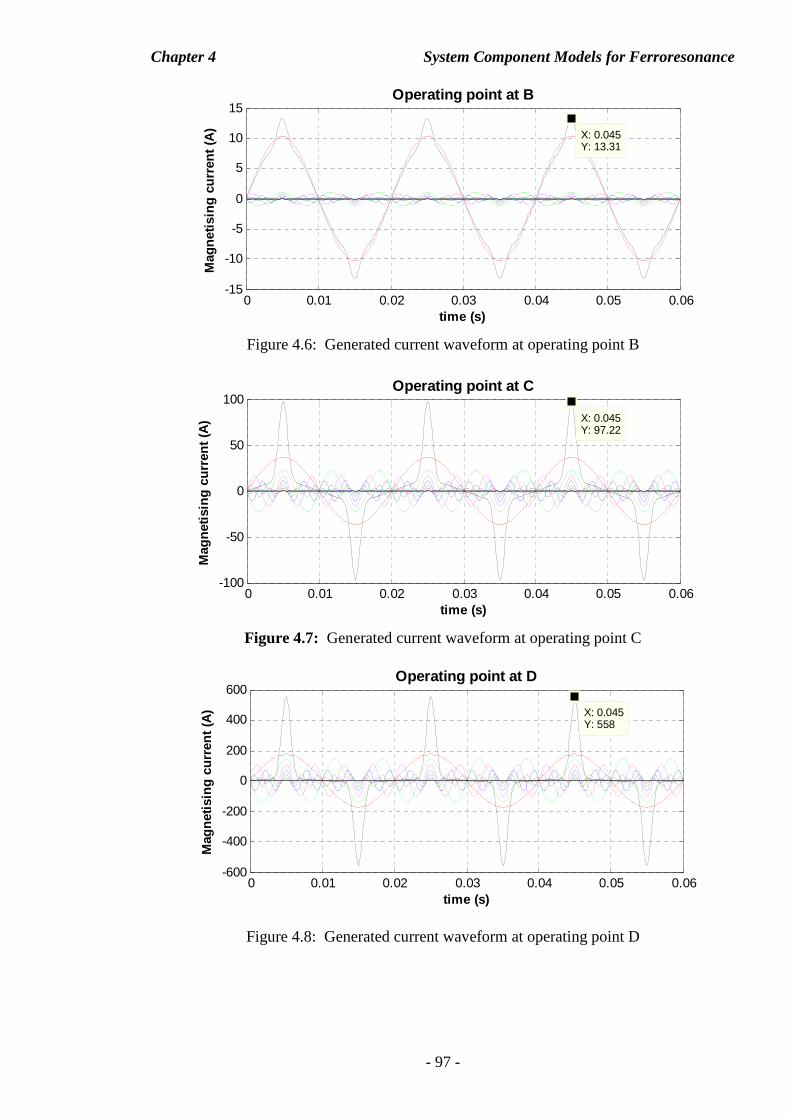
Chapter 4 System Component Models for Ferroresonance
- 97 -
Figure 4.6: Generated current waveform at operating point B
Figure 4.7: Generated current waveform at operating point C
Figure 4.8: Generated current waveform at operating point D
0 0.01 0.02 0.03 0.04 0.05 0.06-15
-10
-5
0
5
10
15Operating point at B
time (s)
Mag
netis
ing
curr
ent (
A) X: 0.045
Y: 13.31
0 0.01 0.02 0.03 0.04 0.05 0.06-100
-50
0
50
100Operating point at C
time (s)
Mag
netis
ing
curr
ent (
A)
X: 0.045Y: 97.22
0 0.01 0.02 0.03 0.04 0.05 0.06-600
-400
-200
0
200
400
600Operating point at D
time (s)
Mag
netis
ing
curr
ent (
A)
X: 0.045Y: 558
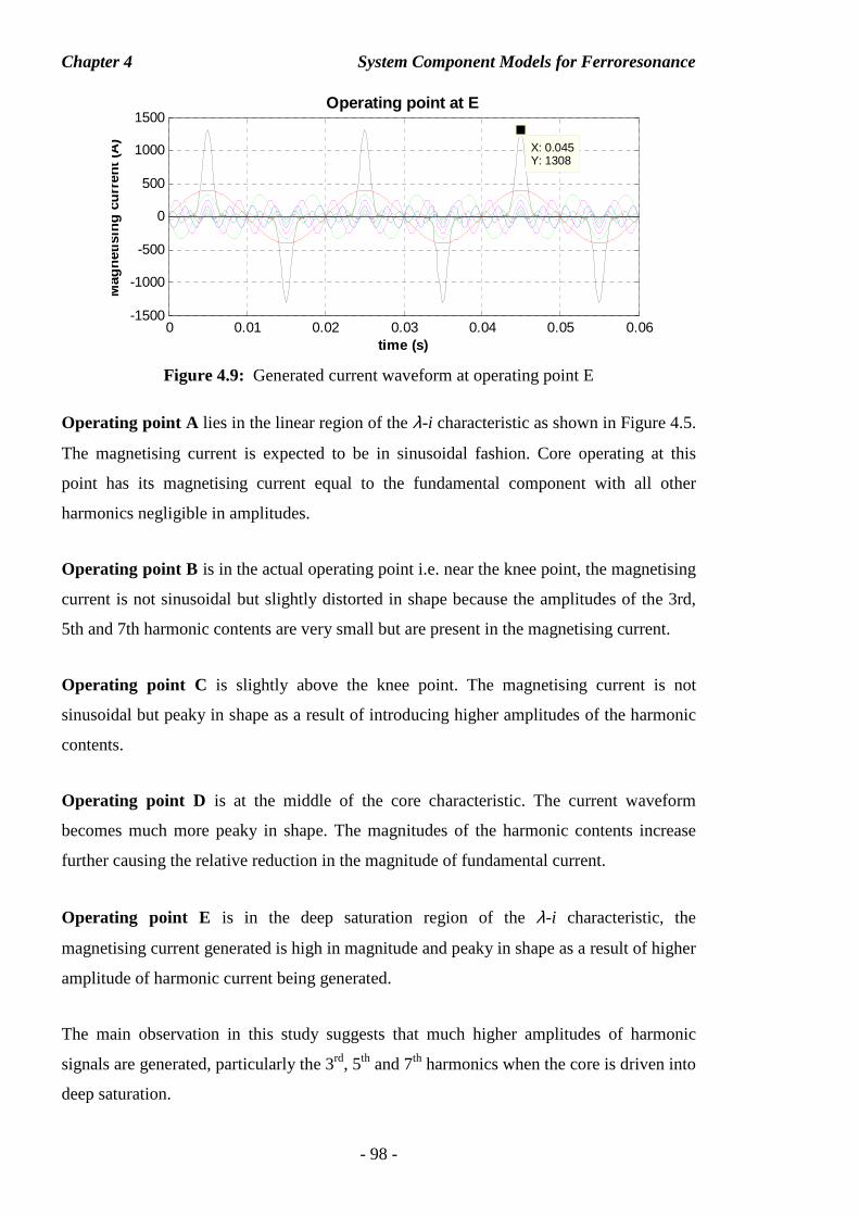
Chapter 4 System Component Models for Ferroresonance
- 98 -
Figure 4.9: Generated current waveform at operating point E
Operating point A lies in the linear region of the λ-i characteristic as shown in Figure 4.5.
The magnetising current is expected to be in sinusoidal fashion. Core operating at this
point has its magnetising current equal to the fundamental component with all other
harmonics negligible in amplitudes.
Operating point B is in the actual operating point i.e. near the knee point, the magnetising
current is not sinusoidal but slightly distorted in shape because the amplitudes of the 3rd,
5th and 7th harmonic contents are very small but are present in the magnetising current.
Operating point C is slightly above the knee point. The magnetising current is not
sinusoidal but peaky in shape as a result of introducing higher amplitudes of the harmonic
contents.
Operating point D is at the middle of the core characteristic. The current waveform
becomes much more peaky in shape. The magnitudes of the harmonic contents increase
further causing the relative reduction in the magnitude of fundamental current.
Operating point E is in the deep saturation region of the λ-i characteristic, the
magnetising current generated is high in magnitude and peaky in shape as a result of higher
amplitude of harmonic current being generated.
The main observation in this study suggests that much higher amplitudes of harmonic
signals are generated, particularly the 3rd, 5th and 7th harmonics when the core is driven into
deep saturation.
0 0.01 0.02 0.03 0.04 0.05 0.06-1500
-1000
-500
0
500
1000
1500Operating point at E
time (s)
Mag
netis
ing
curr
ent (
A) X: 0.045
Y: 1308
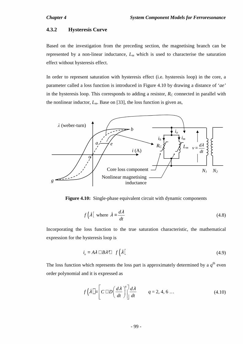
Chapter 4 System Component Models for Ferroresonance
- 99 -
4.3.2 Hysteresis Curve
Based on the investigation from the preceding section, the magnetising branch can be
represented by a non-linear inductance, Lm which is used to characterise the saturation
effect without hysteresis effect.
In order to represent saturation with hysteresis effect (i.e. hysteresis loop) in the core, a
parameter called a loss function is introduced in Figure 4.10 by drawing a distance of ‘ae’
in the hysteresis loop. This corresponds to adding a resistor, RC connected in parallel with
the nonlinear inductor, Lm. Base on [33], the loss function is given as,
Figure 4.10: Single-phase equivalent circuit with dynamic components
( )f λɺ where d
dt
λλ =ɺ (4.8)
Incorporating the loss function to the true saturation characteristic, the mathematical
expression for the hysteresis loop is
( )poi A B fλ λ λ= + + ɺ (4.9)
The loss function which represents the loss part is approximately determined by a qth even
order polynomial and it is expressed as
( )q
d df C D
dt dt
λ λλ = +
ɺ q = 2, 4, 6 … (4.10)
e a
λ (weber-turn) b
o
g
RC
ih
Lm
N1 N2
io
Nonlinear magnetising inductance
im
dt
dv
λ=
Core loss component
i (A)
Chapter 4 System Component Models for Ferroresonance
- 100 -
The total no-load current is
o m h
qp
i i i
d dA B C D
dt dt
λ λλ λ
= +
= + + +
(4.11)
where im is the magnetising current due to magnetic core inductance, and ih is the resistive
current due to hysteresis loss.
The flux linkage is expressed as ( )sinm tλ λ ω= , then ( )cosm
dt
dt
λ λ ω ω= and substituting
into (4.11) then
( ) ( ) ( ) ( ) ( ) ( ) ( ) ( )
1
1
sin sin cos cos
'sin 'sin 'cos 'cos
o m h
p q
m m m m
P q
i i i
A t B t C t D t
A t B t C t D t
λ ω λ ω λ ω ω λ ω ω
ω ω ω ω
+
+
= +
= + + +
= + + +
(4.12)
where ' mA Aλ= , ' pmB Bλ= , ' mC Cλ ω= , 1' ( )q
mD D λ ω +=
The true saturation characteristic is approximated by 27th order polynomial and the loss
part ( )f λɺ is approximated by the qth order polynomial which will be determined by curve
fitting using the power loss equation. The area of the hysteresis loop which determines the
power loss per cycle is given as
( )
( ) ( ) ( ) ( )
( ) ( ) ( )
( ) ( ) ( ) ( )
2
( ) ( )
0
21
0
22 2
0
2 22 2
0 0
1.
2
1cos . 'cos 'cos
2
'cos 'cos2
'cos 'cos2
losses t h t
qm
qm
qm
P v i d t
V t C t D t d t
VC t D t d t
VC t d t D t d t
π
π
π
π π
ωπ
ω ω ω ωπ
ω ω ωπ
ω ω ω ωπ
+
+
+
=
= +
= +
= +
∫
∫
∫
∫ ∫
(4.13)
For the first term, since ( )2 1cos cos 2 1
2θ θ= + and solving it yields,
Chapter 4 System Component Models for Ferroresonance
- 101 -
( ) ( ) ( ) ( ) ( )
( ) ( )
( )( )
2 22
0 0
2
0
2
': 'cos cos 2 1
2 2 2
' 1sin 2
2 2 2
' 2
2 2
'
2
2
m m
m
m
m
m
V V CFirst term C t d t t d t
V Ct t
V C
C V
CV
π π
π
ω ω ω ωπ π
ω ωπ
ππ
= +
= +
=
=
=
∫ ∫
( ) ( ) ( ) ( )
( ) ( )
( )( ) ( )( )( )
2 22 '
0 0
21
20
2
2
': 'cos cos2 2
' 1 1cos sin
2
' 1
2
1 3 5 ...2
2 2 4 ...
q nm m
nmn
mn
qm
V V DSecond term D t d t D t d t
V D nt t I
n n
V D nI
n
n n nDV
n n n
π π
π
ω ω ω ωπ π
ω ωπ
π
ππ
+
−−
−
+
=
− = +
− =
− − −= × − −
∫ ∫
where 2n q= + , ( ) ( )2
22
0
cosnnI t d t
π
ω ω−− = ∫
Note: ( ) ( )2
00
0
cos 2I t d tπ
ω ω π= =∫
Finally, the general core loss is expressed as,
( ) ( ) ( )( )( )( ) ( )( ) ( )( )
22 1 1 3 5 7 ...
2 2 2 4 6 ...qm
losses m
q q q q qCVP DV
q q q q q+ + − − − −
= + + − − − (4.14)
To confirm the correctness of equation (4.14), an example is carried out by deriving the
power equation without using equation (4.14). It is assumed that in a modern transformer,
the true saturation characteristic is approximated by a fifth order polynomial and the loss
part ( )f λɺ approximation by the cubic order, i.e. p = 5 and q = 2. Then,
Chapter 4 System Component Models for Ferroresonance
- 102 -
( )
( ) ( ) ( )
( ) ( ) ( )
( ) ( ) ( ) ( )
2
( ) ( )
0
2' 2 1
0
22 2 2
0
2 22 4
0 0
1.
2
1cos . 'cos cos
2
'cos 'cos2
'cos 'cos2
losses t h t
m
m
m
P v i d t
V t C t D t dt
VC t D t d t
VC t d t D t d t
π
π
π
π π
ωπ
ω ω ωπ
ω ω ωπ
ω ω ω ωπ
+
+
=
= +
= +
= +
∫
∫
∫
∫ ∫
(4.15)
For the first term, since ( )2 1cos cos 2 1
2θ θ= + and solving yields,
( ) ( ) ( ) ( ) ( )
( ) ( )
( )( )
2 22
0 0
2
0
2
': 'cos cos 2 12 2 2
' 1sin 2
2 2 2
' 2
2 2
2
m m
m
m
m
V V CFirst term C t d t t d t
V Ct t
C V
CV
π π
π
ω ω ω ωπ π
ω ωπ
ππ
= +
= +
=
=
∫ ∫
( ) ( ) ( ) ( ) ( ) ( )
( ) ( ) ( ) ( )
( ) ( ) ( )
2 24
0 0
2
0
2
0
4
': 'cos cos 2 1 cos 2 12 2 4
' 1 1cos 4 2cos 2 1
2 4 2 2
' 1 1sin 4 sin 2
2 4 8 2
3
8
m m
m
m
m
V V DSecond term D t d t t t d t
V Dt t d t
V Dt t t t
DV
π π
π
π
ω ω ω ω ωπ π
ω ω ωπ
ω ω ω ωπ
= + +
= + + +
= + + +
=
∫ ∫
∫
Finally, the core-loss is expressed as,
( ) ( ) ( ) ( )
2 22 4
0 0
2 4
' s ' s2
1 3
2 8
mlosses
m m
VP C co t d t D co t d t
CV DV
π π
ω ω ω ωπ
= +
= +
∫ ∫ (4.16)
The power-loss which has been derived in equation (4.16) is proved to be mathematically
correct with the power loss equation (4.14) by using the previous assumptions of p=5 and
q=2 then
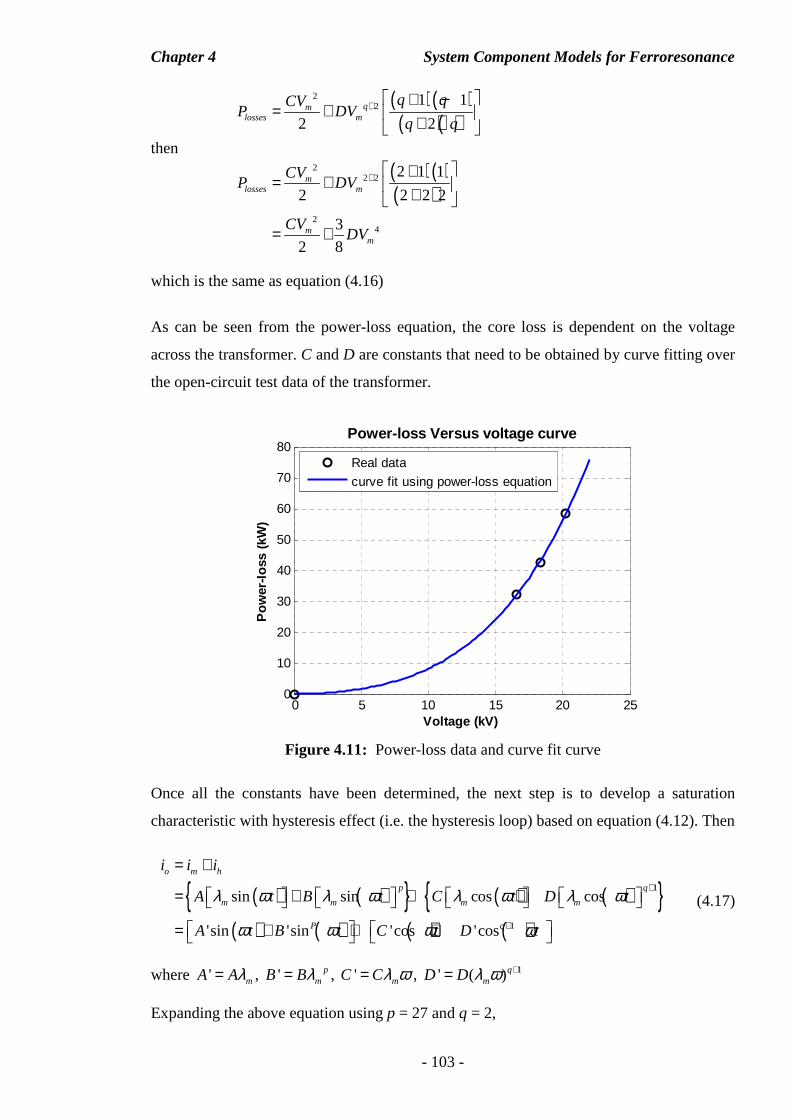
Chapter 4 System Component Models for Ferroresonance
- 103 -
( )( )
( )( )2
2 1 1
2 2qm
losses m
q qCVP DV
q q+ + −
= + +
then
( ) ( )( )
22 2
24
2 1 1
2 2 2 2
3
2 8
mlosses m
mm
CVP DV
CVDV
+ += + +
= +
which is the same as equation (4.16)
As can be seen from the power-loss equation, the core loss is dependent on the voltage
across the transformer. C and D are constants that need to be obtained by curve fitting over
the open-circuit test data of the transformer.
Figure 4.11: Power-loss data and curve fit curve
Once all the constants have been determined, the next step is to develop a saturation
characteristic with hysteresis effect (i.e. the hysteresis loop) based on equation (4.12). Then
( ) ( ) ( ) ( ) ( ) ( ) ( ) ( )
1
1
sin sin cos cos
'sin 'sin 'cos 'cos
o m h
p q
m m m m
P q
i i i
A t B t C t D t
A t B t C t D t
λ ω λ ω λ ω λ ω
ω ω ω ω
+
+
= +
= + + +
= + + +
(4.17)
where ' mA Aλ= , ' pmB Bλ= , ' mC Cλ ω= , 1' ( )q
mD D λ ω +=
Expanding the above equation using p = 27 and q = 2,
0 5 10 15 20 250
10
20
30
40
50
60
70
80Power-loss Versus voltage curve
Voltage (kV)
Pow
er-lo
ss (
kW)
Real data
curve fit using power-loss equation
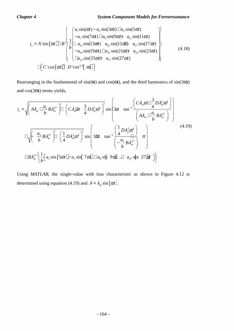
Chapter 4 System Component Models for Ferroresonance
- 104 -
( )
1 3 5
7 9 11
13 15 17
19 21 23
25 27
sin( ) sin(3 ) sin(5 )
sin(7 ) sin(9 ) sin(11 )1
'sin ' sin(13 ) sin(15 ) sin(17 )
sin(19 ) sin(21 ) sin(23 )
sin(25 ) sin(27 )
o
a t a t a t
a t a t a t
i A t B a t a t a tb
a t a t a t
a t a t
ω ω ωω ω ω
ω ω ω ωω ω ωω ω
− + − + − = + + − +
− + − + −
( ) ( )1'cos 'cosqC t D tω ω+
+ +
(4.18)
Rearranging in the fundamental of sin(ωt) and cos(ωt), and the third harmonics of sin(3ωt)
and cos(3ωt) terms yields,
3 32 2
27 3 3 11
271
3 32 2
27 3 3 13
273
27
33 4
sin tan4
11 4
sin 3 tan4
1
m m
o m m m m
m m
m
m m
m
m
C Da
i A B C D tab A Bb
Da
B D tab
Bb
B ab
λ ω λ ωλ λ λ ω λ ω ω
λ λ
λ ωλ λ ω ω π
λ
λ
−
−
+ = + + + + +
+ − + + + −
+ ( ) ( ) ( ) ( )5 7 9 27sin 5 sin 7 sin 9 ... sin 27t a t a t a tω ω ω ω − + +
(4.19)
Using MATLAB, the single-value with loss characteristic as shown in Figure 4.12 is
determined using equation (4.19) and ( )sinm tλ λ ω= .
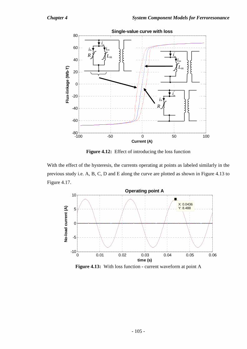
Chapter 4 System Component Models for Ferroresonance
- 105 -
Figure 4.12: Effect of introducing the loss function
With the effect of the hysteresis, the currents operating at points as labeled similarly in the
previous study i.e. A, B, C, D and E along the curve are plotted as shown in Figure 4.13 to
Figure 4.17.
Figure 4.13: With loss function - current waveform at point A
-100 -50 0 50 100-80
-60
-40
-20
0
20
40
60
80Single-value curve with loss
Current (A)
Flu
x-lin
kage
(W
b-T
)
Rih
Lm
im
Lm
'oi
im
R
ih
''oi
oi
0 0.01 0.02 0.03 0.04 0.05 0.06-10
-5
0
5
10Operating point A
time (s)
No-
load
cur
rent
(A
)
X: 0.0436Y: 8.488
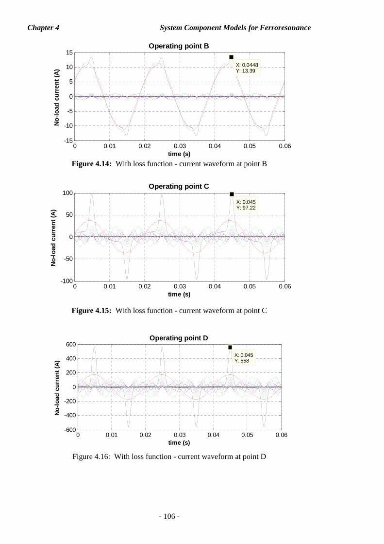
Chapter 4 System Component Models for Ferroresonance
- 106 -
Figure 4.14: With loss function - current waveform at point B
Figure 4.15: With loss function - current waveform at point C
Figure 4.16: With loss function - current waveform at point D
0 0.01 0.02 0.03 0.04 0.05 0.06-15
-10
-5
0
5
10
15Operating point B
time (s)
No-
load
cur
rent
(A
)X: 0.0448Y: 13.39
0 0.01 0.02 0.03 0.04 0.05 0.06-100
-50
0
50
100Operating point C
time (s)
No-
load
cur
rent
(A
)
X: 0.045Y: 97.22
0 0.01 0.02 0.03 0.04 0.05 0.06-600
-400
-200
0
200
400
600Operating point D
time (s)
No-
load
cur
rent
(A
)
X: 0.045Y: 558
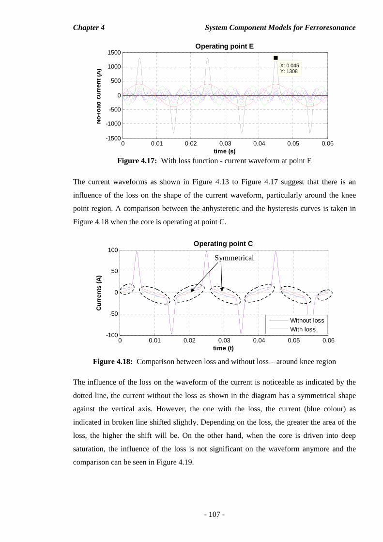
Chapter 4 System Component Models for Ferroresonance
- 107 -
Figure 4.17: With loss function - current waveform at point E
The current waveforms as shown in Figure 4.13 to Figure 4.17 suggest that there is an
influence of the loss on the shape of the current waveform, particularly around the knee
point region. A comparison between the anhysteretic and the hysteresis curves is taken in
Figure 4.18 when the core is operating at point C.
Figure 4.18: Comparison between loss and without loss – around knee region
The influence of the loss on the waveform of the current is noticeable as indicated by the
dotted line, the current without the loss as shown in the diagram has a symmetrical shape
against the vertical axis. However, the one with the loss, the current (blue colour) as
indicated in broken line shifted slightly. Depending on the loss, the greater the area of the
loss, the higher the shift will be. On the other hand, when the core is driven into deep
saturation, the influence of the loss is not significant on the waveform anymore and the
comparison can be seen in Figure 4.19.
0 0.01 0.02 0.03 0.04 0.05 0.06-100
-50
0
50
100Operating point C
time (t)
Cur
rent
s (A
)
Without loss
With loss
Symmetrical
0 0.01 0.02 0.03 0.04 0.05 0.06-1500
-1000
-500
0
500
1000
1500Operating point E
time (s)
No-
load
cur
rent
(A
)
X: 0.045Y: 1308
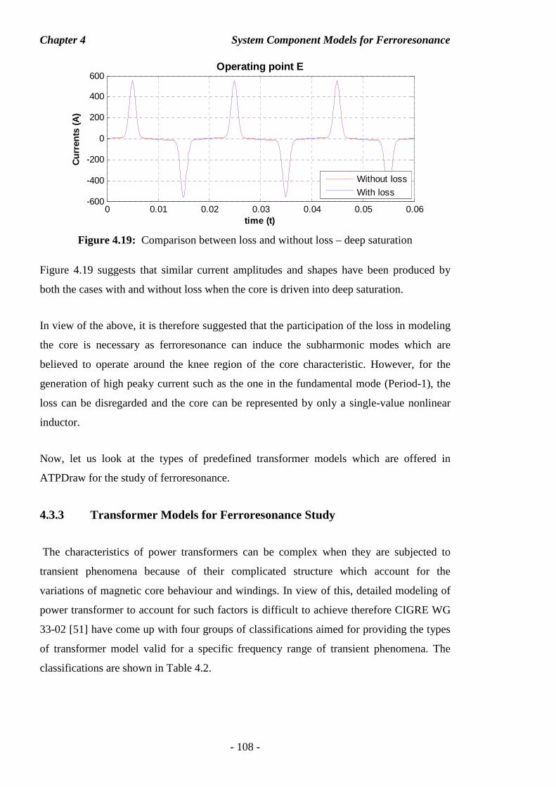
Chapter 4 System Component Models for Ferroresonance
- 108 -
Figure 4.19: Comparison between loss and without loss – deep saturation
Figure 4.19 suggests that similar current amplitudes and shapes have been produced by
both the cases with and without loss when the core is driven into deep saturation.
In view of the above, it is therefore suggested that the participation of the loss in modeling
the core is necessary as ferroresonance can induce the subharmonic modes which are
believed to operate around the knee region of the core characteristic. However, for the
generation of high peaky current such as the one in the fundamental mode (Period-1), the
loss can be disregarded and the core can be represented by only a single-value nonlinear
inductor.
Now, let us look at the types of predefined transformer models which are offered in
ATPDraw for the study of ferroresonance.
4.3.3 Transformer Models for Ferroresonance Study
The characteristics of power transformers can be complex when they are subjected to
transient phenomena because of their complicated structure which account for the
variations of magnetic core behaviour and windings. In view of this, detailed modeling of
power transformer to account for such factors is difficult to achieve therefore CIGRE WG
33-02 [51] have come up with four groups of classifications aimed for providing the types
of transformer model valid for a specific frequency range of transient phenomena. The
classifications are shown in Table 4.2.
0 0.01 0.02 0.03 0.04 0.05 0.06-600
-400
-200
0
200
400
600Operating point E
time (t)
Cur
rent
s (A
)
Without loss
With loss
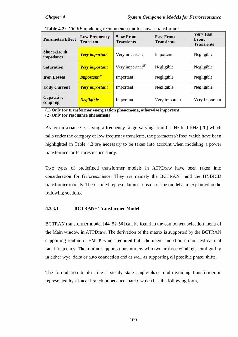
Chapter 4 System Component Models for Ferroresonance
- 109 -
Table 4.2: CIGRE modeling recommendation for power transformer
Parameter/Effect Low Frequency Transients
Slow Front Transients
Fast Front Transients
Very Fast Front Transients
Short-circuit impedance Very important Very important Important Negligible
Saturation Very important Very important(1) Negligible Negligible
Iron Losses Important(2) Important Negligible Negligible
Eddy Current Very important Important Negligible Negligible
Capacitive coupling Negligible Important Very important Very important
(1) Only for transformer energisation phenomena, otherwise important (2) Only for resonance phenomena
As ferroresonance is having a frequency range varying from 0.1 Hz to 1 kHz [20] which
falls under the category of low frequency transients, the parameters/effect which have been
highlighted in Table 4.2 are necessary to be taken into account when modeling a power
transformer for ferroresonance study.
Two types of predefined transformer models in ATPDraw have been taken into
consideration for ferroresonance. They are namely the BCTRAN+ and the HYBRID
transformer models. The detailed representations of each of the models are explained in the
following sections.
4.3.3.1 BCTRAN+ Transformer Model
BCTRAN transformer model [44, 52-56] can be found in the component selection menu of
the Main window in ATPDraw. The derivation of the matrix is supported by the BCTRAN
supporting routine in EMTP which required both the open- and short-circuit test data, at
rated frequency. The routine supports transformers with two or three windings, configuring
in either wye, delta or auto connection and as well as supporting all possible phase shifts.
The formulation to describe a steady state single-phase multi-winding transformer is
represented by a linear branch impedance matrix which has the following form,
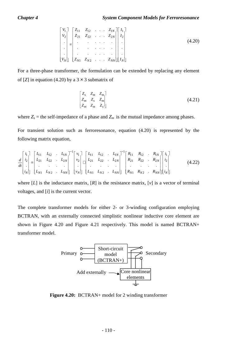
Chapter 4 System Component Models for Ferroresonance
- 110 -
1 11 12 1 1
2 21 22 2 2
1 2
. . .
. . .
. . . . . . . .
. . . . . . . .
. . . . . . . .
. . .
N
N
N N N NN N
V Z Z Z I
V Z Z Z I
V Z Z Z I
=
(4.20)
For a three-phase transformer, the formulation can be extended by replacing any element
of [Z] in equation (4.20) by a 3 × 3 submatrix of
s m m
m s m
m m s
Z Z Z
Z Z Z
Z Z Z
(4.21)
where Zs = the self-impedance of a phase and Zm is the mutual impedance among phases.
For transient solution such as ferroresonance, equation (4.20) is represented by the
following matrix equation,
1 11 11 12 1 1 11 12 1 11 12 1 1
2 21 22 2 2 21 22 2 21 22 2 2
1 2 1 2 1 2
. . .
. . .
. . . . . . . . . . . . . . .
. . .
N N N
N N N
N N N NN N N N NN N N NN
i L L L v L L L R R R i
i L L L v L L L R R R id
dt
i L L L v L L L R R R
− − = + Ni
(4.22)
where [L] is the inductance matrix, [R] is the resistance matrix, [v] is a vector of terminal
voltages, and [i] is the current vector.
The complete transformer models for either 2- or 3-winding configuration employing
BCTRAN, with an externally connected simplistic nonlinear inductive core element are
shown in Figure 4.20 and Figure 4.21 respectively. This model is named BCTRAN+
transformer model.
Figure 4.20: BCTRAN+ model for 2 winding transformer
Primary
Secondary
Short-circuit model
(BCTRAN+)
Core nonlinear elements
Add externally
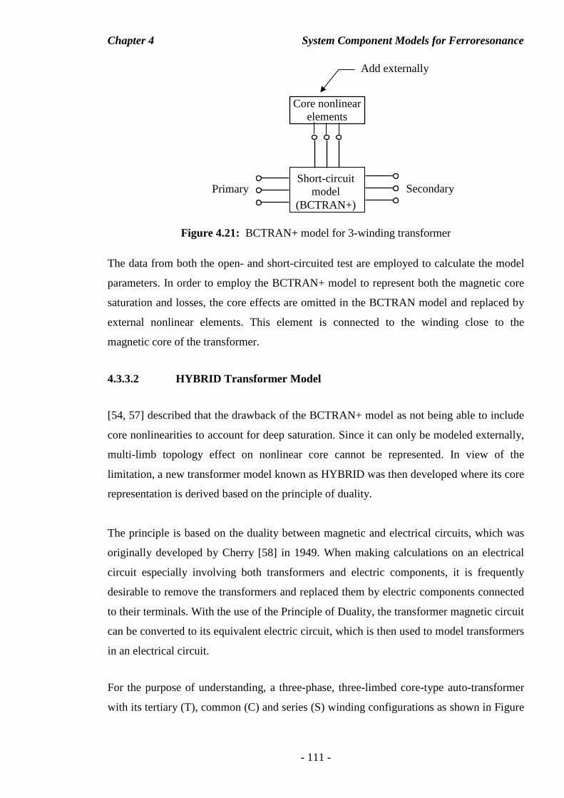
Chapter 4 System Component Models for Ferroresonance
- 111 -
Figure 4.21: BCTRAN+ model for 3-winding transformer
The data from both the open- and short-circuited test are employed to calculate the model
parameters. In order to employ the BCTRAN+ model to represent both the magnetic core
saturation and losses, the core effects are omitted in the BCTRAN model and replaced by
external nonlinear elements. This element is connected to the winding close to the
magnetic core of the transformer.
4.3.3.2 HYBRID Transformer Model
[54, 57] described that the drawback of the BCTRAN+ model as not being able to include
core nonlinearities to account for deep saturation. Since it can only be modeled externally,
multi-limb topology effect on nonlinear core cannot be represented. In view of the
limitation, a new transformer model known as HYBRID was then developed where its core
representation is derived based on the principle of duality.
The principle is based on the duality between magnetic and electrical circuits, which was
originally developed by Cherry [58] in 1949. When making calculations on an electrical
circuit especially involving both transformers and electric components, it is frequently
desirable to remove the transformers and replaced them by electric components connected
to their terminals. With the use of the Principle of Duality, the transformer magnetic circuit
can be converted to its equivalent electric circuit, which is then used to model transformers
in an electrical circuit.
For the purpose of understanding, a three-phase, three-limbed core-type auto-transformer
with its tertiary (T), common (C) and series (S) winding configurations as shown in Figure
Primary
Secondary
Short-circuit model
(BCTRAN+)
Core nonlinear elements
Add externally
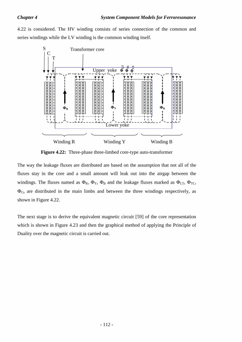
Chapter 4 System Component Models for Ferroresonance
- 112 -
4.22 is considered. The HV winding consists of series connection of the common and
series windings while the LV winding is the common winding itself.
Figure 4.22: Three-phase three-limbed core-type auto-transformer
The way the leakage fluxes are distributed are based on the assumption that not all of the
fluxes stay in the core and a small amount will leak out into the airgap between the
windings. The fluxes named as ΦR, ΦY, ΦB and the leakage fluxes marked as ΦLT, ΦTC,
ΦCs are distributed in the main limbs and between the three windings respectively, as
shown in Figure 4.22.
The next stage is to derive the equivalent magnetic circuit [59] of the core representation
which is shown in Figure 4.23 and then the graphical method of applying the Principle of
Duality over the magnetic circuit is carried out.
ΦB ΦY ΦR
ΦT
C
ΦLT
ΦC
S
Winding R Winding Y Winding B
Upper yoke
Lower yoke
Transformer core
T
S C
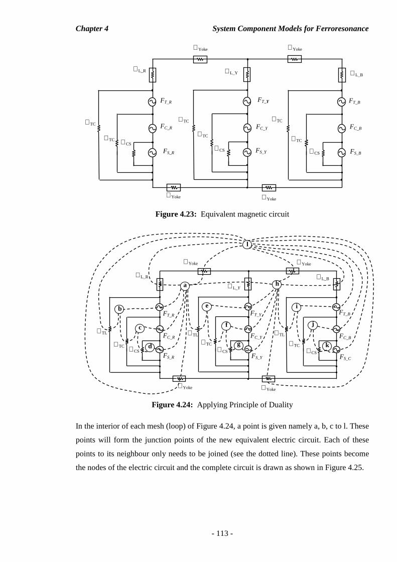
Chapter 4 System Component Models for Ferroresonance
- 113 -
Figure 4.23: Equivalent magnetic circuit
Figure 4.24: Applying Principle of Duality
In the interior of each mesh (loop) of Figure 4.24, a point is given namely a, b, c to l. These
points will form the junction points of the new equivalent electric circuit. Each of these
points to its neighbour only needs to be joined (see the dotted line). These points become
the nodes of the electric circuit and the complete circuit is drawn as shown in Figure 4.25.
ℜYoke ℜYoke
ℜYoke ℜYoke
FS_R
FT_R
FC_R
ℜCS ℜTC
ℜL_Y
ℜCS
ℜTC
ℜTC
ℜL_B
ℜCS
ℜTC
ℜTC
FT_Y
FC_Y
FS_Y
FT_B
FC_B
FS_B
ℜL_R
ℜTC
FS_R
ℜYoke
ℜYoke
FT_R
FC_R
ℜL_R
ℜCS
ℜTL
ℜTC
ℜL_Y
ℜCS
ℜTL
ℜTC
ℜL_B
ℜCS
ℜTL
ℜTC
ℜYoke
FT_Y
FC_Y
FS_Y
FT_B
FC_B
FS_C
a
ℜYoke
b
c
d
e
f
g
h
i
j
k
l
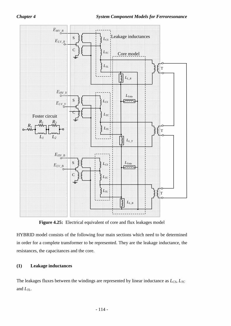
Chapter 4 System Component Models for Ferroresonance
- 114 -
Figure 4.25: Electrical equivalent of core and flux leakages model
HYBRID model consists of the following four main sections which need to be determined
in order for a complete transformer to be represented. They are the leakage inductance, the
resistances, the capacitances and the core.
(1) Leakage inductances
The leakages fluxes between the windings are represented by linear inductance as LCS, LTC
and LTL.
EHV_R
S
C
ELV_R LCS
LTC
LTL T
EHV_Y
S
C
ELV_Y LCS
LTC
LTL T
EHV_B
S
C
ELV_B LCS
LTC
LTL T
LL_R
LL_Y
LL_B
LYoke
LYoke
Core model
Leakage inductances
R1 R2
L1 L2
Rs
Foster circuit
Chapter 4 System Component Models for Ferroresonance
- 115 -
(2) Resistances
The ways the winding resistances are represented in the model are to be added externally at
the terminals of the transformer. Moreover, the resistances can be optionally presented as
frequency dependent which is derived from the Foster circuit. A Foster circuit [51, 59] is
used to represent the resistance of the winding which varies with the frequency of the
current, i.e. the change of resistance of the winding due to the skin effects. Skin effect is
due to the non-uniformly distribution of current in the winding conductor; as frequency
increases, more current flows near the surface of conductor which will increase its
resistance.
(3) Capacitances
External and internal coupling capacitive effects of the transformer are taken into
consideration in the HYBRID model, they include
- Capacitances between windings: primary-to-ground, secondary-to-ground,
primary-to-secondary, tertiary-to-ground, secondary-to-tertiary and tertiary-to-
primary.
- Capacitances between phases performed at primary, secondary and tertiary: Red-
to-yellow phase, yellow-to-blue phase and blue-to-red phase.
(4) Core
The core model is developed by fitting the measured excitation currents and losses. The
user can specify 9 points on the magnetising characteristic to define the air-core for the
transformer.
There are three different sources of data that the HYBRID model can rely on, they are
• Design parameters – Winding and core geometries and material properties.
• Test report – Standard open- and short-circuited test data from the manufacturers.
• Typical values - Typical values based on transformer ratings which can be found in
text books. However, care needs to be taken since both design and material
properties have changed a lot for the past decades.
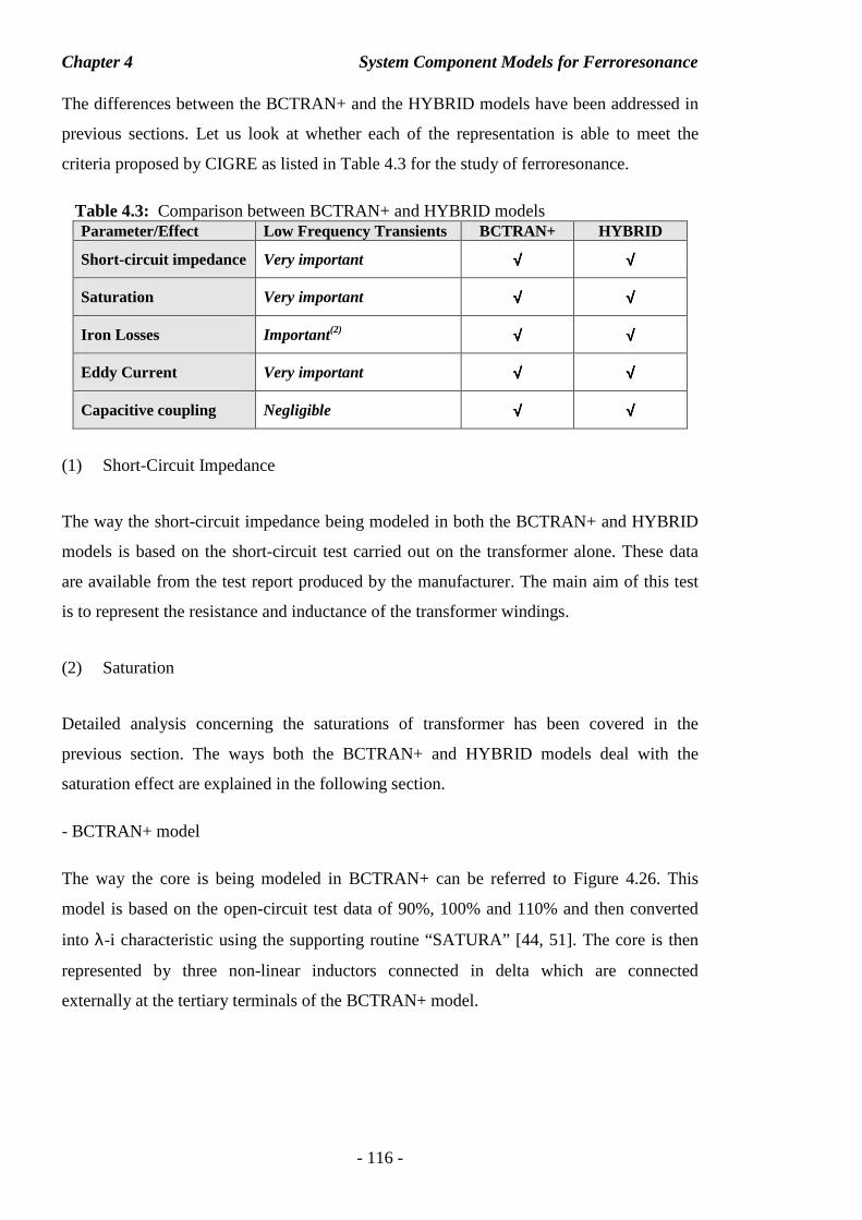
Chapter 4 System Component Models for Ferroresonance
- 116 -
The differences between the BCTRAN+ and the HYBRID models have been addressed in
previous sections. Let us look at whether each of the representation is able to meet the
criteria proposed by CIGRE as listed in Table 4.3 for the study of ferroresonance.
Table 4.3: Comparison between BCTRAN+ and HYBRID models Parameter/Effect Low Frequency Transients BCTRAN+ HYBRID
Short-circuit impedance Very important √√√√ √√√√
Saturation Very important √√√√ √√√√
Iron Losses Important(2) √√√√ √√√√
Eddy Current Very important √√√√ √√√√
Capacitive coupling Negligible √√√√ √√√√
(1) Short-Circuit Impedance
The way the short-circuit impedance being modeled in both the BCTRAN+ and HYBRID
models is based on the short-circuit test carried out on the transformer alone. These data
are available from the test report produced by the manufacturer. The main aim of this test
is to represent the resistance and inductance of the transformer windings.
(2) Saturation
Detailed analysis concerning the saturations of transformer has been covered in the
previous section. The ways both the BCTRAN+ and HYBRID models deal with the
saturation effect are explained in the following section.
- BCTRAN+ model
The way the core is being modeled in BCTRAN+ can be referred to Figure 4.26. This
model is based on the open-circuit test data of 90%, 100% and 110% and then converted
into λ-i characteristic using the supporting routine “SATURA” [44, 51]. The core is then
represented by three non-linear inductors connected in delta which are connected
externally at the tertiary terminals of the BCTRAN+ model.
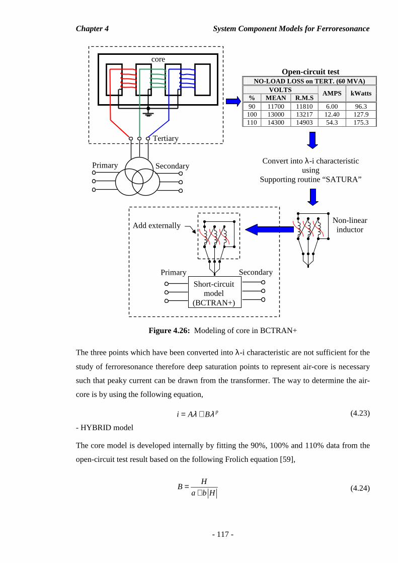
Chapter 4 System Component Models for Ferroresonance
- 117 -
Figure 4.26: Modeling of core in BCTRAN+
The three points which have been converted into λ-i characteristic are not sufficient for the
study of ferroresonance therefore deep saturation points to represent air-core is necessary
such that peaky current can be drawn from the transformer. The way to determine the air-
core is by using the following equation,
pi A Bλ λ= + (4.23)
- HYBRID model
The core model is developed internally by fitting the 90%, 100% and 110% data from the
open-circuit test result based on the following Frolich equation [59],
HB
a b H=
+ (4.24)
Open-circuit test NO-LOAD LOSS on TERT. (60 MVA)
VOLTS % MEAN R.M.S
AMPS kWatts
90 11700 11810 6.00 96.3 100 13000 13217 12.40 127.9 110 14300 14903 54.3 175.3
Primary
core
Tertiary
Secondary
Convert into λ-i characteristic using
Supporting routine “SATURA”
Non-linear inductor
Add externally
Secondary
Primary Short-circuit
model (BCTRAN+)
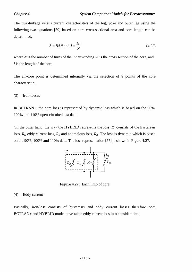
Chapter 4 System Component Models for Ferroresonance
- 118 -
The flux-linkage versus current characteristics of the leg, yoke and outer leg using the
following two equations [59] based on core cross-sectional area and core length can be
determined,
BANλ = and Hl
iN
= (4.25)
where N is the number of turns of the inner winding, A is the cross section of the core, and
l is the length of the core.
The air-core point is determined internally via the selection of 9 points of the core
characteristic.
(3) Iron-losses
In BCTRAN+, the core loss is represented by dynamic loss which is based on the 90%,
100% and 110% open-circuited test data.
On the other hand, the way the HYBRID represents the loss, Rc consists of the hysteresis
loss, RH eddy current loss, RE and anomalous loss, RA. The loss is dynamic which is based
on the 90%, 100% and 110% data. The loss representation [57] is shown in Figure 4.27.
Figure 4.27: Each limb of core
(4) Eddy current
Basically, iron-loss consists of hysteresis and eddy current losses therefore both
BCTRAN+ and HYBRID model have taken eddy current loss into consideration.
RH Lm
im
RE RA
Rc
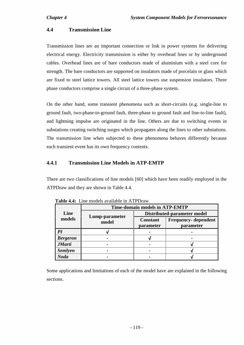
Chapter 4 System Component Models for Ferroresonance
- 119 -
4.4 Transmission Line
Transmission lines are an important connection or link in power systems for delivering
electrical energy. Electricity transmission is either by overhead lines or by underground
cables. Overhead lines are of bare conductors made of aluminium with a steel core for
strength. The bare conductors are supported on insulators made of porcelain or glass which
are fixed to steel lattice towers. All steel lattice towers use suspension insulators. Three
phase conductors comprise a single circuit of a three-phase system.
On the other hand, some transient phenomena such as short-circuits (e.g. single-line to
ground fault, two-phase-to-ground fault, three-phase to ground fault and line-to-line fault),
and lightning impulse are originated in the line. Others are due to switching events in
substations creating switching surges which propagates along the lines to other substations.
The transmission line when subjected to these phenomena behaves differently because
each transient event has its own frequency contents.
4.4.1 Transmission Line Models in ATP-EMTP
There are two classifications of line models [60] which have been readily employed in the
ATPDraw and they are shown in Table 4.4.
Table 4.4: Line models available in ATPDraw Time-domain models in ATP-EMTP
Distributed-parameter model Line models Lump-parameter
model Constant parameter
Frequency- dependent parameter
PI √√√√ - - Bergeron - √√√√ - JMarti - - √√√√ Semlyen - - √√√√ Noda - - √√√√
Some applications and limitations of each of the model have are explained in the following
sections.
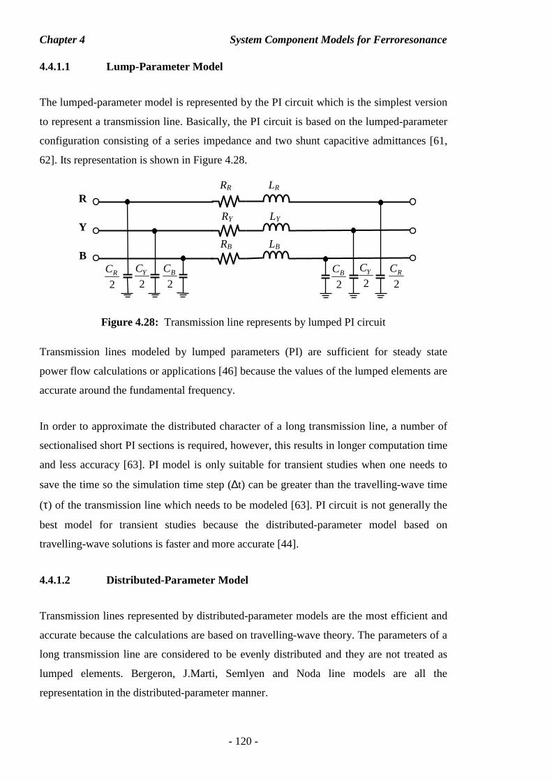
Chapter 4 System Component Models for Ferroresonance
- 120 -
4.4.1.1 Lump-Parameter Model
The lumped-parameter model is represented by the PI circuit which is the simplest version
to represent a transmission line. Basically, the PI circuit is based on the lumped-parameter
configuration consisting of a series impedance and two shunt capacitive admittances [61,
62]. Its representation is shown in Figure 4.28.
Figure 4.28: Transmission line represents by lumped PI circuit
Transmission lines modeled by lumped parameters (PI) are sufficient for steady state
power flow calculations or applications [46] because the values of the lumped elements are
accurate around the fundamental frequency.
In order to approximate the distributed character of a long transmission line, a number of
sectionalised short PI sections is required, however, this results in longer computation time
and less accuracy [63]. PI model is only suitable for transient studies when one needs to
save the time so the simulation time step (∆t) can be greater than the travelling-wave time
(τ) of the transmission line which needs to be modeled [63]. PI circuit is not generally the
best model for transient studies because the distributed-parameter model based on
travelling-wave solutions is faster and more accurate [44].
4.4.1.2 Distributed-Parameter Model
Transmission lines represented by distributed-parameter models are the most efficient and
accurate because the calculations are based on travelling-wave theory. The parameters of a
long transmission line are considered to be evenly distributed and they are not treated as
lumped elements. Bergeron, J.Marti, Semlyen and Noda line models are all the
representation in the distributed-parameter manner.
R
Y
B
RR LR
RY LY
RB LB
2RC
2RC
2YC
2YC
2BC
2BC
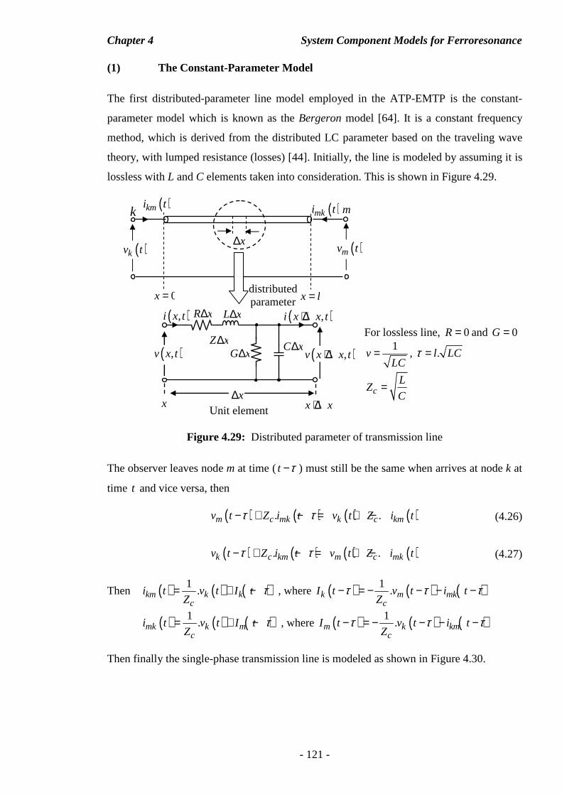
Chapter 4 System Component Models for Ferroresonance
- 121 -
(1) The Constant-Parameter Model
The first distributed-parameter line model employed in the ATP-EMTP is the constant-
parameter model which is known as the Bergeron model [64]. It is a constant frequency
method, which is derived from the distributed LC parameter based on the traveling wave
theory, with lumped resistance (losses) [44]. Initially, the line is modeled by assuming it is
lossless with L and C elements taken into consideration. This is shown in Figure 4.29.
Figure 4.29: Distributed parameter of transmission line
The observer leaves node m at time (t τ− ) must still be the same when arrives at node k at
time t and vice versa, then
( ) ( ) ( ) ( ). .m c mk k c kmv t Z i t v t Z i tτ τ− + − = + − (4.26)
( ) ( ) ( ) ( ). .k c km m c mkv t Z i t v t Z i tτ τ− + − = + − (4.27)
Then ( ) ( ) ( )1.km k k
ci t v t I t
Zτ= + − , where ( ) ( ) ( )1
.k m mkc
I t v t i tZ
τ τ τ− = − − − −
( ) ( ) ( )1.mk k m
ci t v t I t
Zτ= + − , where ( ) ( ) ( )1
.m k kmc
I t v t i tZ
τ τ τ− = − − − −
Then finally the single-phase transmission line is modeled as shown in Figure 4.30.
( )kmi t
For lossless line, 0R = and 0G = 1
vLC
= , .l LCτ =
cL
ZC
=
C x∆
( ),i x t
Unit element
R x∆ L x∆
x∆
( ),v x t
( ),i x x t+ ∆
( ),v x x t+ ∆
x
Z x∆G x∆
x x+ ∆
( )mki tk
( )kv t
m
( )mv t
0x = x l=
x∆
distributed parameter
s
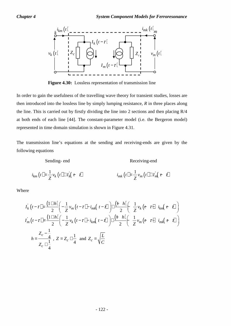
Chapter 4 System Component Models for Ferroresonance
- 122 -
Figure 4.30: Lossless representation of transmission line
In order to gain the usefulness of the travelling wave theory for transient studies, losses are
then introduced into the lossless line by simply lumping resistance, R in three places along
the line. This is carried out by firstly dividing the line into 2 sections and then placing R/4
at both ends of each line [44]. The constant-parameter model (i.e. the Bergeron model)
represented in time domain simulation is shown in Figure 4.31.
The transmission line’s equations at the sending and receiving-ends are given by the
following equations
Sending- end Receiving-end
( ) ( ) ( )'1km k ki t v t I t
Zτ= + − ( ) ( ) ( )'1
mk m mi t v t I tZ
τ= + −
Where
( ) ( ) ( ) ( ) ( ) ( ) ( )' 1 11 1
2 2k m mk k kmh h
I t v t i t v t i tZ Z
τ τ τ τ τ+ − − = − − − − + − − − −
( ) ( ) ( ) ( ) ( ) ( ) ( )' 1 11 1
2 2m k km m mkh h
I t v t i t v t i tZ Z
τ τ τ τ τ+ − − = − − − − + − − − −
1414
c
c
Zh
Z
−=
+ ,
1
4cZ Z= + and cL
ZC
=
cZ
( )kI t τ−
( )kmi t
cZ
( )mI t τ−
( )mki t
( )kv t
k
( )mv t
m
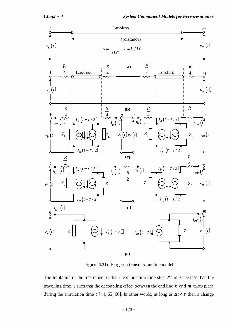
Chapter 4 System Component Models for Ferroresonance
- 123 -
Figure 4.31: Bergeron transmission line model
The limitation of the line model is that the simulation time step, t∆ must be less than the
travelling time, τ such that the decoupling effect between the end line k and m takes place
during the simulation time t [44, 65, 66]. In other words, as long as t τ∆ < then a change
( )/ 2mI t τ−
( )/ 2bI t τ−
cZ
( )bi t
( )bv t
b 4
R
CZ
( )mki t
( )mv t
m 4
R
( )/ 2aI t τ−
( )/ 2kI t τ−
cZ
( )kmi t
( )kv t
k 4
R
cZ
( )ai t
( )av t
a 4
R
4
R
4
R
Lossless 4
R
4
R
Lossless k m
( )kv t ( )mv t
Lossless k m
( )kv t ( )mv t l (distance)
1v
LC= , .l LCτ =
( )/ 2mI t τ−
( )/ 2bI t τ−
cZ
( )bi t
cZ
( )mki t
( )mv t
m 4
R
( )/ 2aI t τ−
( )/ 2kI t τ−
cZ
( )kmi t
( )kv t
k 4
R
cZ
( )ai t
2
R
( )mki t
Z ( )'mI t τ− ( )mv t
m
( )'kI t τ−
( )kmi t
( )kv t
k
Z
(a)
(b)
(c)
(d)
(e)
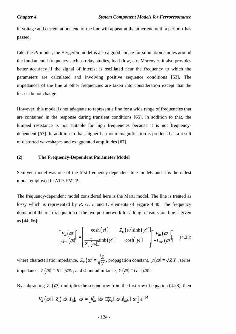
Chapter 4 System Component Models for Ferroresonance
- 124 -
in voltage and current at one end of the line will appear at the other end until a period τ has
passed.
Like the PI model, the Bergeron model is also a good choice for simulation studies around
the fundamental frequency such as relay studies, load flow, etc. Moreover, it also provides
better accuracy if the signal of interest is oscillated near the frequency to which the
parameters are calculated and involving positive sequence conditions [63]. The
impedances of the line at other frequencies are taken into consideration except that the
losses do not change.
However, this model is not adequate to represent a line for a wide range of frequencies that
are contained in the response during transient conditions [65]. In addition to that, the
lumped resistance is not suitable for high frequencies because it is not frequency-
dependent [67]. In addition to that, higher harmonic magnification is produced as a result
of distorted waveshapes and exaggerated amplitudes [67].
(2) The Frequency-Dependent Parameter Model
Semlyen model was one of the first frequency-dependent line models and it is the oldest
model employed in ATP-EMTP.
The frequency-dependent model considered here is the Marti model. The line is treated as
lossy which is represented by R, G, L and C elements of Figure 4.30. The frequency
domain of the matrix equation of the two port network for a long transmission line is given
as [44, 66]:
( )( )
( ) ( ) ( )
( ) ( ) ( )( )( )
cosh sinh
1sinh cosh
ck m
km mkc
l Z lV V
l lI IZ
γ ω γω ω
γ γω ωω
= −
(4.28)
where characteristic impedance, ( )cZ
ZY
ω = , propagation constant, ( ) .Z Yγ ω = , series
impedance, ( )Z R j Lω ω= + , and shunt admittance, ( )Y G j Cω ω= + .
By subtracting ( )cZ ω multiplies the second row from the first row of equation (4.28), then
( ) ( ) ( ) ( ) ( ) ( ). . . lk c km m c mkV Z I V Z I e γω ω ω ω ω ω −− = +
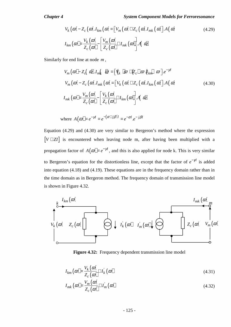
Chapter 4 System Component Models for Ferroresonance
- 125 -
( ) ( ) ( ) ( ) ( ) ( ) ( ). . .k c km m c mkV Z I V Z I Aω ω ω ω ω ω ω− = + (4.29)
( ) ( )( )
( )( ) ( ) ( ).k m
km mkc c
V VI I A
Z Z
ω ωω ω ω
ω ω
= − +
Similarly for end line at node m ,
( ) ( ) ( ) ( ) ( ) ( ). . . lm c mk k c kmV Z I V Z I e γω ω ω ω ω ω −− = +
( ) ( ) ( ) ( ) ( ) ( ) ( ). . .m c mk k c kmV Z I V Z I Aω ω ω ω ω ω ω− = + (4.30)
( ) ( )( )
( )( ) ( ) ( ).m k
mk kmc c
V VI I A
Z Z
ω ωω ω ω
ω ω
= − +
where ( ) ( ) .j ll l j lA e e e eα βγ α βω − +− − −= = =
Equation (4.29) and (4.30) are very similar to Bergeron’s method where the expression
[ ]V ZI+ is encountered when leaving node m, after having been multiplied with a
propagation factor of ( ) lA e γω −= , and this is also applied for node k. This is very similar
to Bergeron’s equation for the distortionless line, except that the factor of le γ− is added
into equation (4.18) and (4.19). These equations are in the frequency domain rather than in
the time domain as in Bergeron method. The frequency domain of transmission line model
is shown in Figure 4.32.
Figure 4.32: Frequency dependent transmission line model
( ) ( )( ) ( )'k
km kc
VI I
Z
ωω ω
ω= + (4.31)
( ) ( )( ) ( )'m
mk mc
VI I
Z
ωω ω
ω= + (4.32)
( )mkI ω
( )cZ ω ( )'mI ω ( )mV ω
m
( )'kI ω
( )kmI ω
( )kV ω
k
( )cZ ω
Chapter 4 System Component Models for Ferroresonance
- 126 -
where ( ) ( )( ) ( ) ( )' .m
k mkc
VI I A
Z
ωω ω ω
ω
= +
, ( ) ( )( ) ( ) ( )' .k
m kmc
VI I A
Z
ωω ω ω
ω
= +
,
( ) lA e γω −=
Since time domain solutions are required in the EMTP simulation, therefore the frequency
domain of Equation (4.31) and (4.32) are then converted into the time domain by using the
convolution integral.
Let,
( ) ( ) ( ) ( ).k k c kmB V Z Iω ω ω ω= − , ( ) ( ) ( ) ( ).m m c mkB V Z Iω ω ω ω= −
( ) ( ) ( ) ( ).m m c mkF V Z Iω ω ω ω= + , ( ) ( ) ( ) ( ).k k c kmF V Z Iω ω ω ω= +
Equation (4.31) and (4.32) become
( ) ( ) ( ).k mB F Aω ω ω= (4.33)
( ) ( ) ( ).m kB F Aω ω ω= (4.34)
Applying convolution integral to equation (4.33) and (4.34) then,
( ) ( ).mF Aω ω ⇔⇔⇔⇔ ( ) ( ) ( )t
m mf a t f t u a u duτ
⊗ = −∫
( ) ( ).kF Aω ω ⇔⇔⇔⇔ ( ) ( ) ( )t
k kf a t f t u a u duτ
⊗ = −∫
However, the above method involves lengthy process of evaluating the convolution
integral therefore an alternative approximate approach i.e. a rational function suggested by
Marti [66] is best to approximate ( ) lA e γω −= which has the following term,
( ) ( ) 1 2
1 2
. . .s l smapprox
m
kk kA s e e
s p s p s pγ τ− −
= = + + + + + + (4.35)
Then in time-domain form as
( ) ( ) ( ) ( )1 min 2 min min
1 2 . . . mp t p t p tapprox mA t k e k e k eτ τ τ− − − − − −= + + + for mint τ≥
0= for mint τ≤
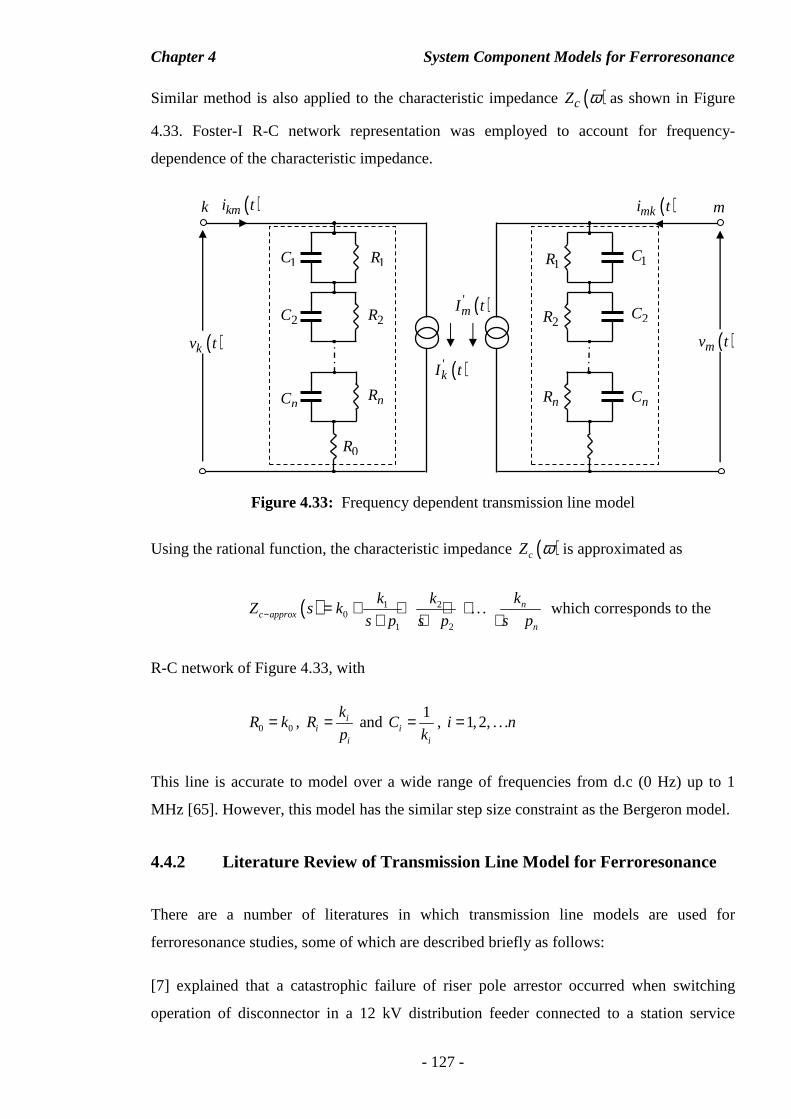
Chapter 4 System Component Models for Ferroresonance
- 127 -
Similar method is also applied to the characteristic impedance ( )cZ ω as shown in Figure
4.33. Foster-I R-C network representation was employed to account for frequency-
dependence of the characteristic impedance.
Figure 4.33: Frequency dependent transmission line model
Using the rational function, the characteristic impedance ( )cZ ω is approximated as
( ) 1 20
1 2
. . . nc approx
n
kk kZ s k
s p s p s p− = + + + ++ + +
which corresponds to the
R-C network of Figure 4.33, with
0 0R k= , ii
i
kR
p= and
1i
i
Ck
= , 1,2, . . .i n=
This line is accurate to model over a wide range of frequencies from d.c (0 Hz) up to 1
MHz [65]. However, this model has the similar step size constraint as the Bergeron model.
4.4.2 Literature Review of Transmission Line Model for Ferroresonance
There are a number of literatures in which transmission line models are used for
ferroresonance studies, some of which are described briefly as follows:
[7] explained that a catastrophic failure of riser pole arrestor occurred when switching
operation of disconnector in a 12 kV distribution feeder connected to a station service
( )mki t
( )'mI t
( )mv t
m
( )kmi t
( )kv t
k
1C
2C
nC
1R
2R
nR
0R
1C
2C
nC
1R
2R
nR
( )'kI t
Chapter 4 System Component Models for Ferroresonance
- 128 -
transformer has been carried out. The simulation study is modeled using ATP-EMTP. For
the component modeling, the overhead line has been modeled as PI model.
[68] mentioned that ferroresonance occurred when a no-load transformer was energised by
adjacent live line via capacitive coupling of the double-circuit transmission line. In the
simulation model, the transposed transmission line has been modeled by using a frequency
dependent line model.
[24] described that a blackout event has occurred at their nuclear power station because of
ferroresonant overvoltages being induced into the system. The aim of building a simulation
model of the affected system is to determine if the simulation results matched with the
actual recording results such that the root cause of the problem can be investigated. The
transmission line was modeled by connecting several identical PI divisions to represent an
approximate model of distributed parameter line.
[5] explained the modeling work which has been performed to validate the actual
ferroresonance field measurements. The transmission line involved in the system is a
double-circuit with un-transposed configuration. The type of line modeled in ATP-EMTP
has been based on a Bergeron model.
Paper on ‘Modeling and Analysis Guidelines for Slow Transients-Part III: The Study of
Ferroresonance’ [69] quoted that either the distributed line or the cascaded PI model for
long line can be employed for ferroresonance study.
There is no specific type of line model which has been proposed or suggested for
ferroresonance study after surveying some of the literatures. Therefore assessment
procedure has been developed to evaluate the type of line model that is suitable for
ferroresonance study.
4.4.3 Handling of Simulation Time, ∆∆∆∆t
It is important to choose the correct simulation time step before a simulation case study is
carried out in ATPDraw to avoid simulation errors. Therefore, the main aim of this section
is to aid users to handle the simulation time-step i.e. ∆t when either the lumped- or the
distributed-parameter transmission lines is chosen for ferroresonance study. A flowchart as
shown in Figure 4.34 has been setup for this purpose.
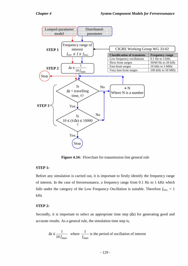
Chapter 4 System Component Models for Ferroresonance
- 129 -
Figure 4.34: Flowchart for transmission line general rule
STEP 1:
Before any simulation is carried out, it is important to firstly identify the frequency range
of interest. In the case of ferroresonance, a frequency range from 0.1 Hz to 1 kHz which
falls under the category of the Low Frequency Oscillation is suitable. Therefore fmax. = 1
kHz
STEP 2:
Secondly, it is important to select an appropriate time step (∆t) for generating good and
accurate results. As a general rule, the simulation time step is,
max
1
10t
f∆ ≤ where
max
1
fis the period of oscillation of interest
Distributed-parameter
model
max
1
10t
f∆ ≤
Frequency range of interest
fmin ≤ f ≤ fmax.
Is ∆t < travelling
time, τ?
No
Yes
Stop
Is 10 ≤ (τ/∆t) ≤ 10000
?
No
Yes
CIGRE Working Group WG 33-02
÷÷÷÷ N Where N is a number
Lumped-parameter model
Stop
Classification of transients Frequency range Low frequency oscillations 0.1 Hz to 3 kHz Slow-front surges 50/60 Hz to 20 kHz Fast-front surges 10 kHz to 3 MHz Very-fast-front surges 100 kHz to 50 MHz
STEP 1
STEP 2
STEP 3
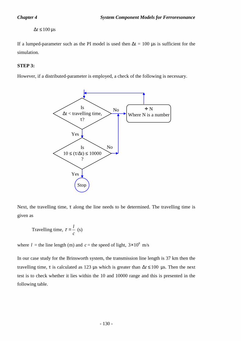
Chapter 4 System Component Models for Ferroresonance
- 130 -
100t∆ ≤ µs
If a lumped-parameter such as the PI model is used then ∆t = 100 µs is sufficient for the
simulation.
STEP 3:
However, if a distributed-parameter is employed, a check of the following is necessary.
Next, the travelling time, τ along the line needs to be determined. The travelling time is
given as
Travelling time, l
cτ = (s)
where l = the line length (m) and c= the speed of light, 83 10× m/s
In our case study for the Brinsworth system, the transmission line length is 37 km then the
travelling time, τ is calculated as 123 µs which is greater than 100t∆ ≤ µs. Then the next
test is to check whether it lies within the 10 and 10000 range and this is presented in the
following table.
Is ∆t < travelling time,
τ?
No
Yes
Stop
Is 10 ≤ (τ/∆t) ≤ 10000
?
No
Yes
÷÷÷÷ N Where N is a number
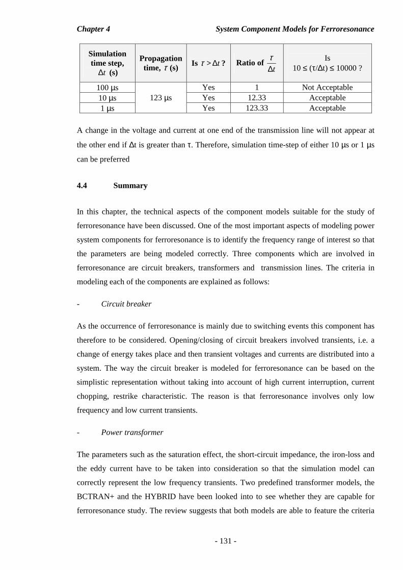
Chapter 4 System Component Models for Ferroresonance
- 131 -
Simulation time step,
t∆ (s)
Propagation time, τ (s) Is τ > t∆ ? Ratio of
t
τ∆
Is
10 ≤ (τ/∆t) ≤ 10000 ?
100 µs Yes 1 Not Acceptable 10 µs Yes 12.33 Acceptable 1 µs
123 µs Yes 123.33 Acceptable
A change in the voltage and current at one end of the transmission line will not appear at
the other end if ∆t is greater than τ. Therefore, simulation time-step of either 10 µs or 1 µs
can be preferred
4.4 Summary
In this chapter, the technical aspects of the component models suitable for the study of
ferroresonance have been discussed. One of the most important aspects of modeling power
system components for ferroresonance is to identify the frequency range of interest so that
the parameters are being modeled correctly. Three components which are involved in
ferroresonance are circuit breakers, transformers and transmission lines. The criteria in
modeling each of the components are explained as follows:
- Circuit breaker
As the occurrence of ferroresonance is mainly due to switching events this component has
therefore to be considered. Opening/closing of circuit breakers involved transients, i.e. a
change of energy takes place and then transient voltages and currents are distributed into a
system. The way the circuit breaker is modeled for ferroresonance can be based on the
simplistic representation without taking into account of high current interruption, current
chopping, restrike characteristic. The reason is that ferroresonance involves only low
frequency and low current transients.
- Power transformer
The parameters such as the saturation effect, the short-circuit impedance, the iron-loss and
the eddy current have to be taken into consideration so that the simulation model can
correctly represent the low frequency transients. Two predefined transformer models, the
BCTRAN+ and the HYBRID have been looked into to see whether they are capable for
ferroresonance study. The review suggests that both models are able to feature the criteria

Chapter 4 System Component Models for Ferroresonance
- 132 -
(parameter/effect) for low frequency transients, hence for ferroresonance. In addition
BCTRAN+ and HYBRID models are valid for up to 2 kHz and 5 kHz respectively. The
only difference between the two is the way in which the core is taken into consideration.
- Transmission line
Again, frequency range of interest needs to be determined so that a proper predefined
model can be used. The three predefined models, the PI, Bergeron and the Marti are
considered to be adequate for modeling ferroresonance. For a short-line up to less than 50
km, a PI model is considered to be adequate for ferroresonance. Bergeron model is a
constant frequency method, based on traveling wave theory, and can also be used for
ferroresonance study. On the other hand, transmission line represented by the J. Marti
model can also be used for ferroresonance study because the parameters of the line are
frequency-dependent which can cover up to 1 MHz.
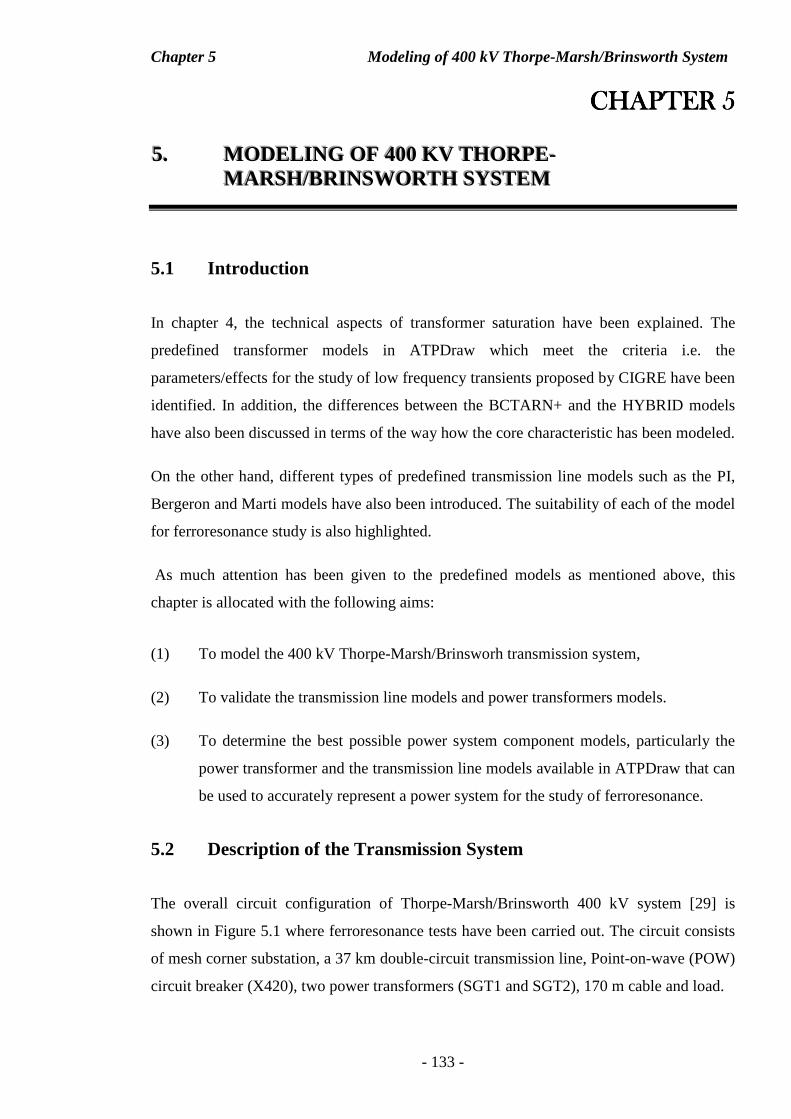
Chapter 5 Modeling of 400 kV Thorpe-Marsh/Brinsworth System
- 133 -
CHAPTER 5 CHAPTER 5 CHAPTER 5 CHAPTER 5
555... MMM OOODDDEEELLL III NNNGGG OOOFFF 444000000 KKK VVV TTTHHHOOORRRPPPEEE--- MMM AAARRRSSSHHH///BBBRRRIII NNNSSSWWWOOORRRTTTHHH SSSYYYSSSTTTEEEMMM
5.1 Introduction
In chapter 4, the technical aspects of transformer saturation have been explained. The
predefined transformer models in ATPDraw which meet the criteria i.e. the
parameters/effects for the study of low frequency transients proposed by CIGRE have been
identified. In addition, the differences between the BCTARN+ and the HYBRID models
have also been discussed in terms of the way how the core characteristic has been modeled.
On the other hand, different types of predefined transmission line models such as the PI,
Bergeron and Marti models have also been introduced. The suitability of each of the model
for ferroresonance study is also highlighted.
As much attention has been given to the predefined models as mentioned above, this
chapter is allocated with the following aims:
(1) To model the 400 kV Thorpe-Marsh/Brinsworh transmission system,
(2) To validate the transmission line models and power transformers models.
(3) To determine the best possible power system component models, particularly the
power transformer and the transmission line models available in ATPDraw that can
be used to accurately represent a power system for the study of ferroresonance.
5.2 Description of the Transmission System
The overall circuit configuration of Thorpe-Marsh/Brinsworth 400 kV system [29] is
shown in Figure 5.1 where ferroresonance tests have been carried out. The circuit consists
of mesh corner substation, a 37 km double-circuit transmission line, Point-on-wave (POW)
circuit breaker (X420), two power transformers (SGT1 and SGT2), 170 m cable and load.
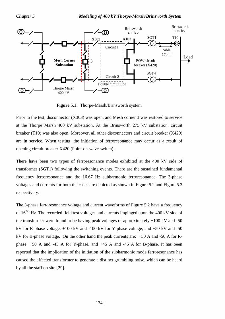
Chapter 5 Modeling of 400 kV Thorpe-Marsh/Brinsworth System
- 134 -
Figure 5.1: Thorpe-Marsh/Brinsworth system
Prior to the test, disconnector (X303) was open, and Mesh corner 3 was restored to service
at the Thorpe Marsh 400 kV substation. At the Brinsworth 275 kV substation, circuit
breaker (T10) was also open. Moreover, all other disconnectors and circuit breaker (X420)
are in service. When testing, the initiation of ferroresonance may occur as a result of
opening circuit breaker X420 (Point-on-wave switch).
There have been two types of ferroresonance modes exhibited at the 400 kV side of
transformer (SGT1) following the switching events. There are the sustained fundamental
frequency ferroresonance and the 16.67 Hz subharmonic ferroresonance. The 3-phase
voltages and currents for both the cases are depicted as shown in Figure 5.2 and Figure 5.3
respectively.
The 3-phase ferroresonance voltage and current waveforms of Figure 5.2 have a frequency
of 162/3 Hz. The recorded field test voltages and currents impinged upon the 400 kV side of
the transformer were found to be having peak voltages of approximately +100 kV and -50
kV for R-phase voltage, +100 kV and -100 kV for Y-phase voltage, and +50 kV and -50
kV for B-phase voltage. On the other hand the peak currents are: +50 A and -50 A for R-
phase, +50 A and -45 A for Y-phase, and +45 A and -45 A for B-phase. It has been
reported that the implication of the initiation of the subharmonic mode ferroresonance has
caused the affected transformer to generate a distinct grumbling noise, which can be heard
by all the staff on site [29].
Load
SGT1
SGT4
Brinsworth 400 kV
POW circuit breaker (X420)
X103
T10
Brinsworth 275 kV
cable 170 m
Thorpe Marsh 400 kV
X303
Mesh Corner Substation
Double circuit line
Circuit 1
Circuit 2
3
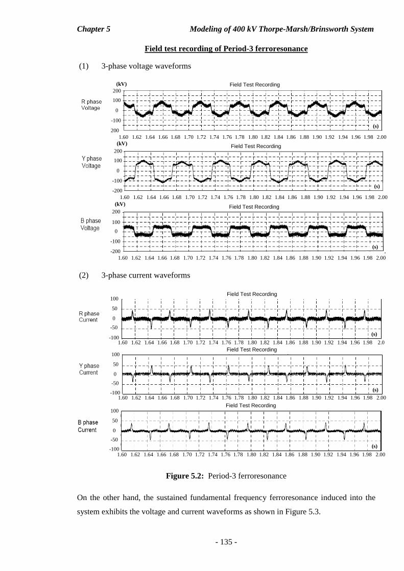
Chapter 5 Modeling of 400 kV Thorpe-Marsh/Brinsworth System
- 135 -
Field test recording of Period-3 ferroresonance
(1) 3-phase voltage waveforms
(2) 3-phase current waveforms
Figure 5.2: Period-3 ferroresonance
On the other hand, the sustained fundamental frequency ferroresonance induced into the
system exhibits the voltage and current waveforms as shown in Figure 5.3.
-50
50
100
-100
0
1.60 1.62 1.64 1.66 1.68 1.70 1.72 1.74 1.76 1.78 1.80 1.82 1.84 1.86 1.88 1.90 1.92 1.94 1.96 1.98 2.0
Field Test Recording
(s)
-50
50
100
-100
0
(s)
Field Test Recording
1.60 1.62 1.64 1.66 1.68 1.70 1.72 1.74 1.76 1.78 1.80 1.82 1.84 1.86 1.88 1.90 1.92 1.94 1.96 1.98 2.00
-50
50
100
-100
0
(s)
1.60 1.62 1.64 1.66 1.68 1.70 1.72 1.74 1.76 1.78 1.80 1.82 1.84 1.86 1.88 1.90 1.92 1.94 1.96 1.98 2.00
Field Test Recording
(s)
Field Test Recording
100 200
200
0
-100
1.60 1.62 1.64 1.66 1.68 1.70 1.72 1.74 1.76 1.78 1.80 1.82 1.84 1.86 1.88 1.90 1.92 1.94 1.96 1.98 2.00
(s)
Field Test Recording (kV)
100 200
-200
0
-100
1.60 1.62 1.64 1.66 1.68 1.70 1.72 1.74 1.76 1.78 1.80 1.82 1.84 1.86 1.88 1.90 1.92 1.94 1.96 1.98 2.00
(s)
Field Test Recording (kV)
100 200
-200
0
-100
1.60 1.62 1.64 1.66 1.68 1.70 1.72 1.74 1.76 1.78 1.80 1.82 1.84 1.86 1.88 1.90 1.92 1.94 1.96 1.98 2.00
(kV)
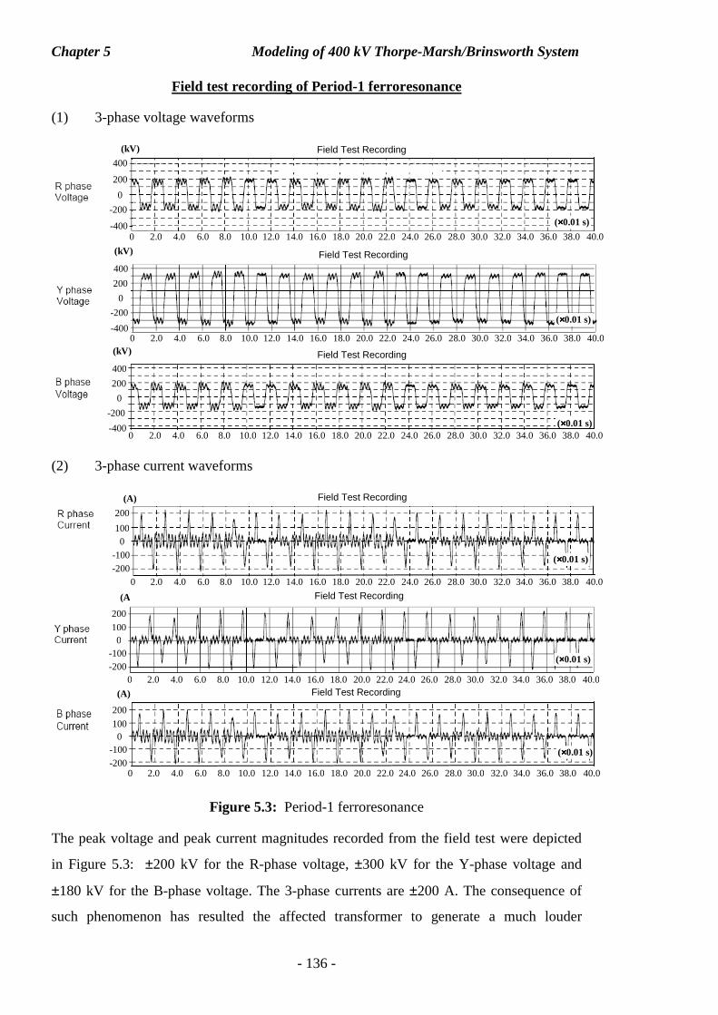
Chapter 5 Modeling of 400 kV Thorpe-Marsh/Brinsworth System
- 136 -
Field test recording of Period-1 ferroresonance
(1) 3-phase voltage waveforms
(2) 3-phase current waveforms
Figure 5.3: Period-1 ferroresonance
The peak voltage and peak current magnitudes recorded from the field test were depicted
in Figure 5.3: ±200 kV for the R-phase voltage, ±300 kV for the Y-phase voltage and
±180 kV for the B-phase voltage. The 3-phase currents are ±200 A. The consequence of
such phenomenon has resulted the affected transformer to generate a much louder
0 2.0 4.0 6.0 8.0 10.0 12.0 14.0 16.0 18.0 20.0 22.0 24.0 26.0 28.0 30.0 32.0 34.0 36.0 38.0 40.0
100 200
0
-200 -100
Field Test Recording (A)
(××××0.01 s)
100 200
0
-200 -100
(A)
0 2.0 4.0 6.0 8.0 10.0 12.0 14.0 16.0 18.0 20.0 22.0 24.0 26.0 28.0 30.0 32.0 34.0 36.0 38.0 40.0
(××××0.01 s)
Field Test Recording
100 200
0
-200 -100
Field Test Recording (A)
0 2.0 4.0 6.0 8.0 10.0 12.0 14.0 16.0 18.0 20.0 22.0 24.0 26.0 28.0 30.0 32.0 34.0 36.0 38.0 40.0
(××××0.01 s)
200 400
0
-400
-200
0 2.0 4.0 6.0 8.0 10.0 12.0 14.0 16.0 18.0 20.0 22.0 24.0 26.0 28.0 30.0 32.0 34.0 36.0 38.0 40.0
Field Test Recording (kV)
(××××0.01 s)
0 2.0 4.0 6.0 8.0 10.0 12.0 14.0 16.0 18.0 20.0 22.0 24.0 26.0 28.0 30.0 32.0 34.0 36.0 38.0 40.0
Field Test Recording (kV)
200 400
-400
-200
0
(××××0.01 s)
0 2.0 4.0 6.0 8.0 10.0 12.0 14.0 16.0 18.0 20.0 22.0 24.0 26.0 28.0 30.0 32.0 34.0 36.0 38.0 40.0 (××××0.01 s)
Field Test Recording (kV)
200 400
-400
0
-200
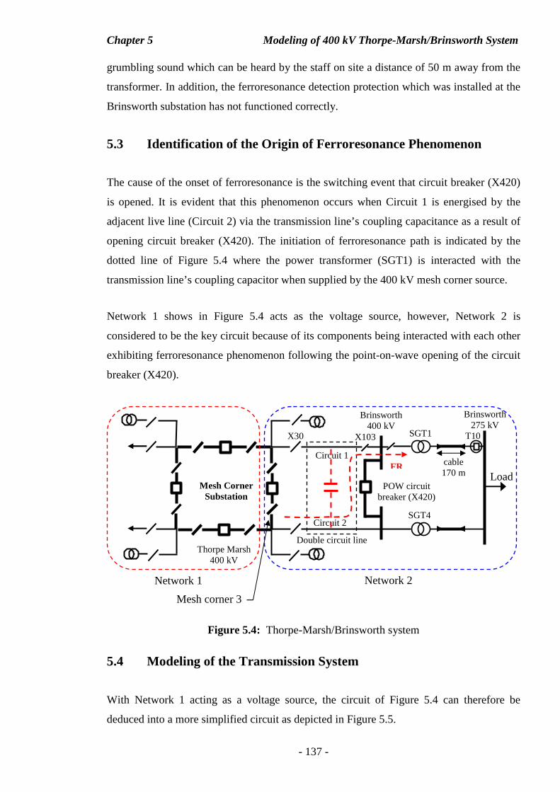
Chapter 5 Modeling of 400 kV Thorpe-Marsh/Brinsworth System
- 137 -
grumbling sound which can be heard by the staff on site a distance of 50 m away from the
transformer. In addition, the ferroresonance detection protection which was installed at the
Brinsworth substation has not functioned correctly.
5.3 Identification of the Origin of Ferroresonance Phenomenon
The cause of the onset of ferroresonance is the switching event that circuit breaker (X420)
is opened. It is evident that this phenomenon occurs when Circuit 1 is energised by the
adjacent live line (Circuit 2) via the transmission line’s coupling capacitance as a result of
opening circuit breaker (X420). The initiation of ferroresonance path is indicated by the
dotted line of Figure 5.4 where the power transformer (SGT1) is interacted with the
transmission line’s coupling capacitor when supplied by the 400 kV mesh corner source.
Network 1 shows in Figure 5.4 acts as the voltage source, however, Network 2 is
considered to be the key circuit because of its components being interacted with each other
exhibiting ferroresonance phenomenon following the point-on-wave opening of the circuit
breaker (X420).
Figure 5.4: Thorpe-Marsh/Brinsworth system
5.4 Modeling of the Transmission System
With Network 1 acting as a voltage source, the circuit of Figure 5.4 can therefore be
deduced into a more simplified circuit as depicted in Figure 5.5.
Mesh corner 3
Load
SGT1
SGT4
Brinsworth 400 kV
POW circuit breaker (X420)
X103
T10
Brinsworth 275 kV
cable 170 m
Thorpe Marsh 400 kV
X30
Mesh Corner Substation
Double circuit line
Circuit 1
Circuit 2
FR
Network 1 Network 2
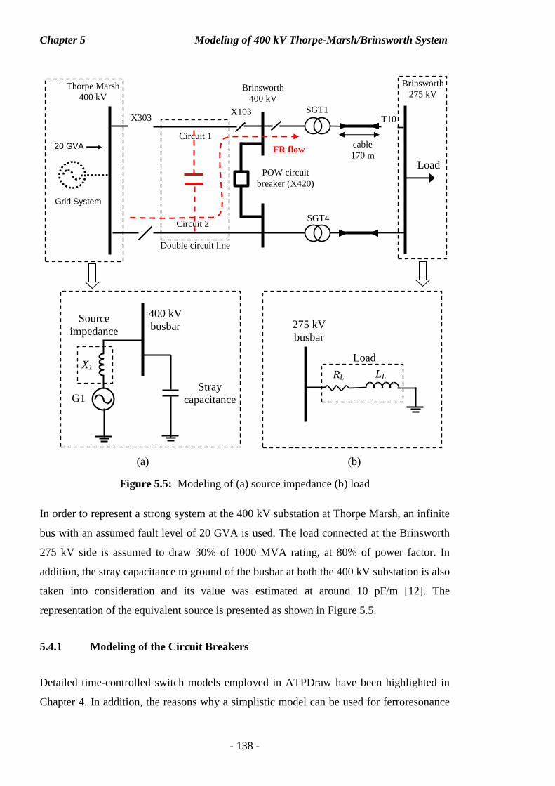
Chapter 5 Modeling of 400 kV Thorpe-Marsh/Brinsworth System
- 138 -
Figure 5.5: Modeling of (a) source impedance (b) load
In order to represent a strong system at the 400 kV substation at Thorpe Marsh, an infinite
bus with an assumed fault level of 20 GVA is used. The load connected at the Brinsworth
275 kV side is assumed to draw 30% of 1000 MVA rating, at 80% of power factor. In
addition, the stray capacitance to ground of the busbar at both the 400 kV substation is also
taken into consideration and its value was estimated at around 10 pF/m [12]. The
representation of the equivalent source is presented as shown in Figure 5.5.
5.4.1 Modeling of the Circuit Breakers
Detailed time-controlled switch models employed in ATPDraw have been highlighted in
Chapter 4. In addition, the reasons why a simplistic model can be used for ferroresonance
Load
SGT1
SGT4
Brinsworth 400 kV
POW circuit breaker (X420)
X103 T10
Brinsworth 275 kV
cable 170 m
X303
Double circuit line
Circuit 1
Circuit 2
FR flow
Thorpe Marsh 400 kV
20 GVA
Grid System
G1
X1
Stray capacitance
L
Source impedance
400 kV busbar
RL LL
Load
275 kV busbar
(a) (b)
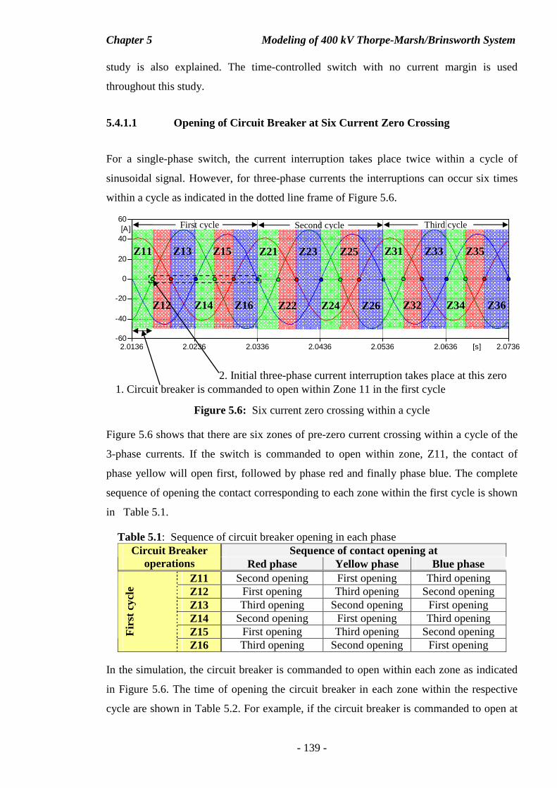
Chapter 5 Modeling of 400 kV Thorpe-Marsh/Brinsworth System
- 139 -
study is also explained. The time-controlled switch with no current margin is used
throughout this study.
5.4.1.1 Opening of Circuit Breaker at Six Current Zero Crossing
For a single-phase switch, the current interruption takes place twice within a cycle of
sinusoidal signal. However, for three-phase currents the interruptions can occur six times
within a cycle as indicated in the dotted line frame of Figure 5.6.
Figure 5.6: Six current zero crossing within a cycle
Figure 5.6 shows that there are six zones of pre-zero current crossing within a cycle of the
3-phase currents. If the switch is commanded to open within zone, Z11, the contact of
phase yellow will open first, followed by phase red and finally phase blue. The complete
sequence of opening the contact corresponding to each zone within the first cycle is shown
in Table 5.1.
Table 5.1: Sequence of circuit breaker opening in each phase Sequence of contact opening at Circuit Breaker
operations Red phase Yellow phase Blue phase Z11 Second opening First opening Third opening Z12 First opening Third opening Second opening Z13 Third opening Second opening First opening Z14 Second opening First opening Third opening Z15 First opening Third opening Second opening F
irst c
ycle
Z16 Third opening Second opening First opening
In the simulation, the circuit breaker is commanded to open within each zone as indicated
in Figure 5.6. The time of opening the circuit breaker in each zone within the respective
cycle are shown in Table 5.2. For example, if the circuit breaker is commanded to open at
2.0136 2.0236 2.0336 2.0436 2.0536 2.0636 2.0736[s]-60
-40
-20
0
20
40
60[A] First cycle
Z11
Z12
Z13
Z14
Z15
Z16
Second cycle
Z21
Z22
Z23
Z24
Z25
Z26
Third cycle
Z31
Z32
Z33
Z34
Z35
Z36
1. Circuit breaker is commanded to open within Zone 11 in the first cycle 2. Initial three-phase current interruption takes place at this zero
Chapter 5 Modeling of 400 kV Thorpe-Marsh/Brinsworth System
- 140 -
2.0153 s at zone Z11 within the 1st cycle, the circuit breaker will not open instantly, instead
it waits until the first current zero crossing takes place which occurs at phase yellow,
follows by current interruptions at red and blue phases.
Table 5.2: Switching time to command the circuit breaker to open 1st cycle
Z11 Z12 Z13 Z14 Z15 Z16 Time to command CB to open
2.0153 s 2.0181 s 2.0219 s 2.0254 s 2.0283 s 2.0319 s
2nd cycle Z21 Z22 Z23 Z24 Z25 Z26 Time to command CB to open
2.0353 s 2.0381 s 2.0419 s 2.0454 s 2.0483 s 2.0519 s
3rd cycle Z31 Z32 Z33 Z34 Z35 Z36 Time to command CB to open
2.0553 s 2.0581 s 2.0619 s 2.0654 s 2.0683 s 2.0719 s
Occasionally, the simulations to reproduce the expected waveforms cannot be extended for
more than three cycles due to the fact that the initial three-phase currents and voltages at
the point of current interruption of each phase are not repetitive from one cycle to another
cycle which can be seen in Table 5.3. Although the differences of the initial conditions are
small, they determine the initial stored energy in the capacitive and inductive components
of the ferroresonant circuit, therefore affect the transient ferroresonant voltages and
currents. As we have known, the transient ferroresonance can develop into sustained
ferroresonance sometimes and also can decay down into zero.
Table 5.3: Sequence of circuit breaker opening in each phase 1st Cycle
Current Z11 Z12 Z13 Z14 Z15 Z16
Red phase
34.083 A (1.6143E5 V)
Interrupted at 2.0198 s
(3.2033E5 V)
-39.647 A (1.2435E5 V)
-33 929 A (-1.6318E5 V)
Interrupted at 2.0298 s
(-3.2041E5 V)
39.682 A (-1.2342E5 V)
Yellow phase
Interrupted at 2.0167 s
(-3.2194E5 V)
41.222 A (-1.8287E5 V)
40.362 A (1.9468E5 V)
Interrupted at 2.0268 s
(3.2193E5 V)
-41.301 A (1.8204E5 V)
-40.253 A (-1.9548E5 V)
Blue phase
-36.731 A (1.6137E5 V)
-42.151 A (-1.373E5 V)
Interrupted at 2.0238 s
(-3.1986E5 V)
36.912 A (-1.5961E5 V)
42.092 A (1.3821E5 V)
Interrupted at 2.0338 s
3.1974E5 V)
2nd Cycle Current
Z21 Z22 Z23 Z24 Z25 Z26 Red
phase 34.602 A
(1.5528E5 V)
Interrupted at 2.0398 s
(3.2056E5 V)
-39.718 A (1.2249E5 V)
-33.696 A (-1.6578E5 V)
Interrupted at 2.0498 s
(-3.2063E5 V)
39.807 A (-1.2062E5 V
Yellow phase
Interrupted at 2.0367 s
(-3.2188E5 V)
41.518 A (-1.8036E5 V)
40.139 A (1.9628E5 V)
Interrupted at 2.0468 s
(3.2189E5 V)
-41.599 A (1.7953E5 V)
-39.976 A (-1.9788E5 V)
Blue phase
-36.157 A (1.6746E5)
-42.021 A (-1.4004E5 V)
Interrupted at 2.0438 s
(-3.1961E5 V)
37.147 A (-1.5697E5 V)
41.967 A (1.4095E5 V)
Interrupted at 2.0538 s
(3.1934E5 V)
Continue…
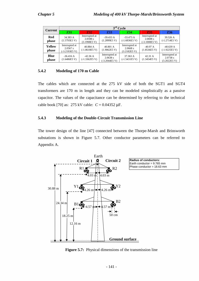
Chapter 5 Modeling of 400 kV Thorpe-Marsh/Brinsworth System
- 141 -
3rd Cycle
Current Z31 Z32 Z33 Z34 Z35 Z36
Red phase
34.383 A (1.5793E5 V)
Interrupted at 2.0598 s
(3.1998E5 V)
-39.433 A (1.2899E5 V)
-33.473 A (-1.6836E5 V)
Interrupted at 2.0698 s
(-3.1008E5 V)
39.526 A (-1.2714E5 V)
Yellow phase
Interrupted at 2.0567 s
(-3.2193E5 V)
40.884 A (-1.8618E5 V)
40.801 A (1.9062E5 V)
Interrupted at 2.0668 s
(3.2182E5 V)
-40.97 A (1.8536E5 V)
-40.639 A (-1.9225E5 V)
Blue phase
-36.416 A (1.6486E5 V)
-42.36 A (-1.3362E5 V)
Interrupted at 2.0638 s
(-3.2044E5 V)
37.363 A (-1.5431E5 V)
42.31 A (1.3454E5 V)
Interrupted at 2.0738 s
(3.2022E5 V)
5.4.2 Modeling of 170 m Cable
The cables which are connected at the 275 kV side of both the SGT1 and SGT4
transformers are 170 m in length and they can be modeled simplistically as a passive
capacitor. The values of the capacitance can be determined by referring to the technical
cable book [70] as: 275 kV cable: C = 0.04352 µF.
5.4.3 Modeling of the Double-Circuit Transmission Line
The tower design of the line [47] connected between the Thorpe-Marsh and Brinsworth
substations is shown in Figure 5.7. Other conductor parameters can be referred to
Appendix A.
Figure 5.7: Physical dimensions of the transmission line
Earth
Ground surface
12.16 m
18.25 m
24.34 m
30.88 m
R1 R2
4.03 m 4.03 m
Y1 Y2 4.26 m 4.26 m
B1 B2
4.57 m 4.57 m
50 cm
Circuit 1 Circuit 2 Radius of conductors: Earth conductor = 9.765 mm Phase conductor = 18.63 mm
Chapter 5 Modeling of 400 kV Thorpe-Marsh/Brinsworth System
- 142 -
The line is modeled in ATPDraw using the integrated LCC object according to the
available physical dimensions and parameters.
Since the main aim of this chapter is to determine the best possible model for
ferroresonance study, therefore, three different types of approaches are put into test to
determine their suitability for the purpose.
5.4.3.1 Lumped Parameter Model
Detailed description about the lumped parameter, particularly the PI model has been
highlighted in the previous chapter. The double-circuit transmission line is modeled in this
representation and the next stage of verifying and checking is shown in Appendix B.
5.4.3.2 Distributed Parameter
Other than the line being modeled in lumped representation, two alternative approaches
based on distributed parameter are also considered with an aim to determine the best
possible model, the Bergeron and J. Marti models. The detailed of each of them have been
explained in the previous chapter.
5.4.4 Modeling of Transformers SGT1 and SGT4
Two power transformers are involved in the transmission system but only SGT1 is affected
by ferroresonance therefore it is modeled by using both BCTRAN+ and HYBRID models
with an aim to determine the best possible model. On the other hand, SGT4 is not affected
by ferroresonance therefore it is only modeled as a steady-state characteristic using
BCTRAN. The open- and short-circuit test data obtained from the test report supplying by
the manufacturers [71] are shown in Table 5.4. The electrical specification of the SGT1
transformer is 1000 MVA, 400/275/13 kV, Vector: YNa0d11 (5 legs). Zero-sequence data
are not available.
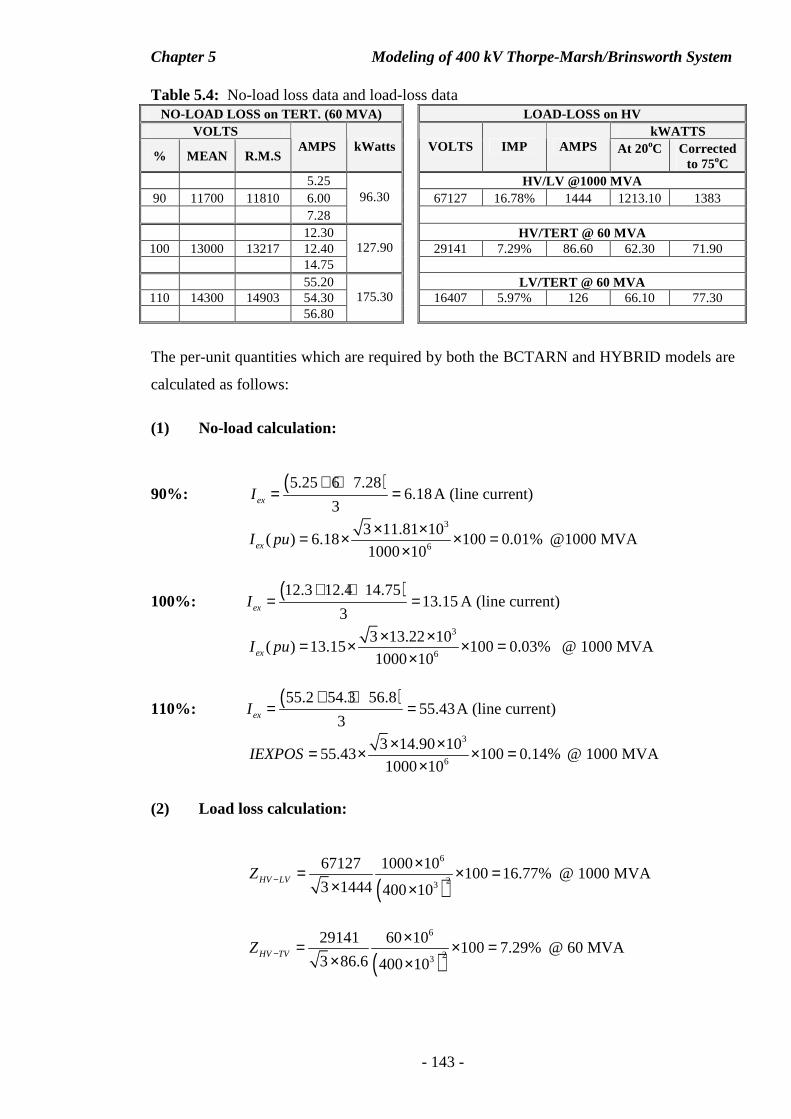
Chapter 5 Modeling of 400 kV Thorpe-Marsh/Brinsworth System
- 143 -
Table 5.4: No-load loss data and load-loss data NO-LOAD LOSS on TERT. (60 MVA) LOAD-LOSS on HV
VOLTS kWATTS
% MEAN R.M.S AMPS kWatts VOLTS IMP AMPS At 20oC Corrected
to 75oC 5.25 HV/LV @1000 MVA
90 11700 11810 6.00 67127 16.78% 1444 1213.10 1383 7.28
96.30
12.30 HV/TERT @ 60 MVA
100 13000 13217 12.40 29141 7.29% 86.60 62.30 71.90 14.75
127.90
55.20 LV/TERT @ 60 MVA 110 14300 14903 54.30 16407 5.97% 126 66.10 77.30
56.80 175.30
The per-unit quantities which are required by both the BCTARN and HYBRID models are
calculated as follows:
(1) No-load calculation:
90%: ( )5.25 6 7.28
6.183exI
+ += = A (line current)
3
6
3 11.81 10( ) 6.18 100 0.01%
1000 10exI pu× ×= × × =
× @1000 MVA
100%: ( )12.3 12.4 14.75
13.153exI
+ += = A (line current)
3
6
3 13.22 10( ) 13.15 100 0.03%
1000 10exI pu× ×= × × =
× @ 1000 MVA
110%: ( )55.2 54.3 56.8
55.433exI
+ += = A (line current)
3
6
3 14.90 1055.43 100 0.14%
1000 10IEXPOS
× ×= × × =×
@ 1000 MVA
(2) Load loss calculation:
( )6
23
67127 1000 10100 16.77%
3 1444 400 10HV LVZ −
×= × =× ×
@ 1000 MVA
( )6
23
29141 60 10100 7.29%
3 86.6 400 10HV TVZ −
×= × =× ×
@ 60 MVA
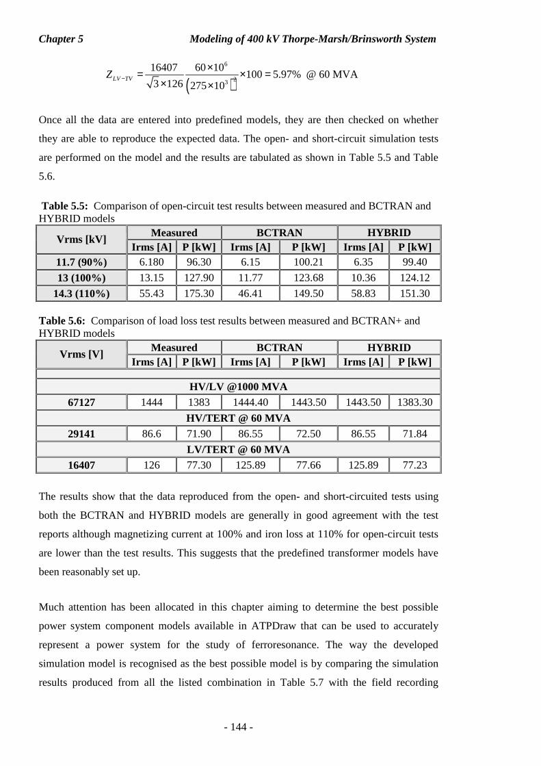
Chapter 5 Modeling of 400 kV Thorpe-Marsh/Brinsworth System
- 144 -
( )6
23
16407 60 10100 5.97%
3 126 275 10LV TVZ −
×= × =× ×
@ 60 MVA
Once all the data are entered into predefined models, they are then checked on whether
they are able to reproduce the expected data. The open- and short-circuit simulation tests
are performed on the model and the results are tabulated as shown in Table 5.5 and Table
5.6.
Table 5.5: Comparison of open-circuit test results between measured and BCTRAN and HYBRID models
Measured BCTRAN HYBRID Vrms [kV]
Irms [A] P [kW] Irms [A] P [kW] Irms [A] P [kW] 11.7 (90%) 6.180 96.30 6.15 100.21 6.35 99.40
13 (100%) 13.15 127.90 11.77 123.68 10.36 124.12
14.3 (110%) 55.43 175.30 46.41 149.50 58.83 151.30 Table 5.6: Comparison of load loss test results between measured and BCTRAN+ and HYBRID models
Measured BCTRAN HYBRID Vrms [V]
Irms [A] P [kW] Irms [A] P [kW] Irms [A] P [kW]
HV/LV @1000 MVA 67127 1444 1383 1444.40 1443.50 1443.50 1383.30
HV/TERT @ 60 MVA 29141 86.6 71.90 86.55 72.50 86.55 71.84
LV/TERT @ 60 MVA 16407 126 77.30 125.89 77.66 125.89 77.23
The results show that the data reproduced from the open- and short-circuited tests using
both the BCTRAN and HYBRID models are generally in good agreement with the test
reports although magnetizing current at 100% and iron loss at 110% for open-circuit tests
are lower than the test results. This suggests that the predefined transformer models have
been reasonably set up.
Much attention has been allocated in this chapter aiming to determine the best possible
power system component models available in ATPDraw that can be used to accurately
represent a power system for the study of ferroresonance. The way the developed
simulation model is recognised as the best possible model is by comparing the simulation
results produced from all the listed combination in Table 5.7 with the field recording
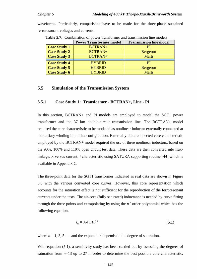
Chapter 5 Modeling of 400 kV Thorpe-Marsh/Brinsworth System
- 145 -
waveforms. Particularly, comparisons have to be made for the three-phase sustained
ferroresonant voltages and currents.
Table 5.7: Combination of power transformer and transmission line models Power Transformer model Transmission line model Case Study 1 BCTRAN+ PI Case Study 2 BCTRAN+ Bergeron Case Study 3 BCTRAN+ Marti
Case Study 4 HYBRID PI Case Study 5 HYBRID Bergeron Case Study 6 HYBRID Marti
5.5 Simulation of the Transmission System
5.5.1 Case Study 1: Transformer - BCTRAN+, Line - PI
In this section, BCTRAN+ and PI models are employed to model the SGT1 power
transformer and the 37 km double-circuit transmission line. The BCTRAN+ model
required the core characteristic to be modeled as nonlinear inductor externally connected at
the tertiary winding in a delta configuration. Externally delta-connected core characteristic
employed by the BCTRAN+ model required the use of three nonlinear inductors, based on
the 90%, 100% and 110% open circuit test data. These data are then converted into flux-
linkage, λ versus current, i characteristic using SATURA supporting routine [44] which is
available in Appendix C.
The three-point data for the SGT1 transformer indicated as real data are shown in Figure
5.8 with the various converted core curves. However, this core representation which
accounts for the saturation effect is not sufficient for the reproduction of the ferroresonant
currents under the tests. The air-core (fully saturated) inductance is needed by curve fitting
through the three points and extrapolating by using the nth order polynomial which has the
following equation,
nmi A Bλ λ= + (5.1)
where n = 1, 3, 5 . . . and the exponent n depends on the degree of saturation.
With equation (5.1), a sensitivity study has been carried out by assessing the degrees of
saturation from n=13 up to 27 in order to determine the best possible core characteristic.
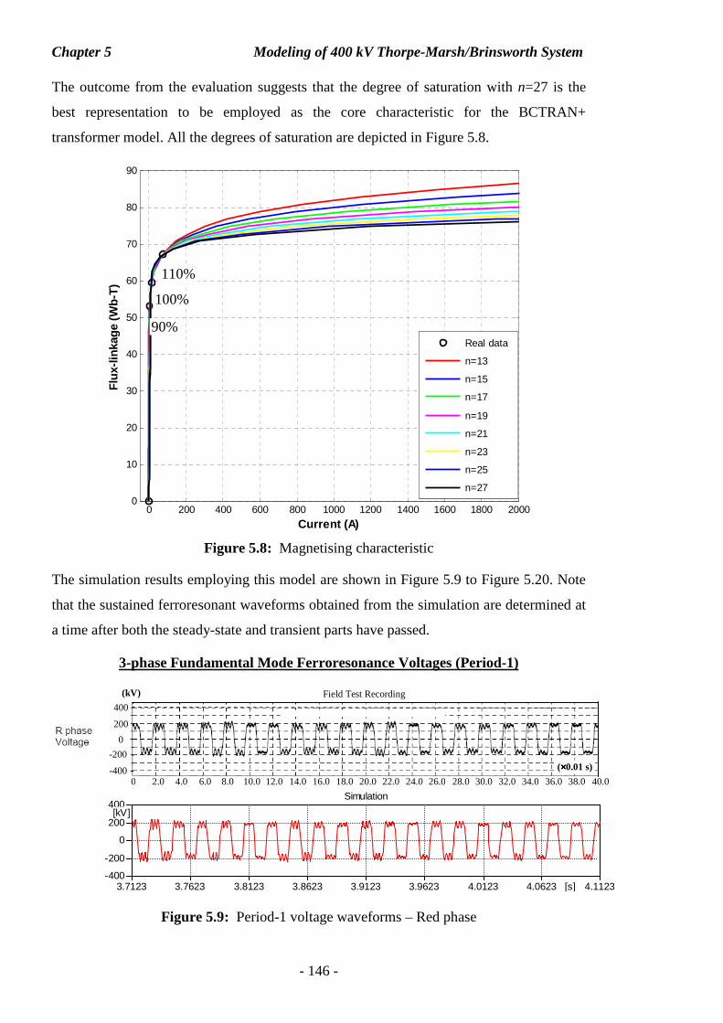
Chapter 5 Modeling of 400 kV Thorpe-Marsh/Brinsworth System
- 146 -
The outcome from the evaluation suggests that the degree of saturation with n=27 is the
best representation to be employed as the core characteristic for the BCTRAN+
transformer model. All the degrees of saturation are depicted in Figure 5.8.
Figure 5.8: Magnetising characteristic
The simulation results employing this model are shown in Figure 5.9 to Figure 5.20. Note
that the sustained ferroresonant waveforms obtained from the simulation are determined at
a time after both the steady-state and transient parts have passed.
3-phase Fundamental Mode Ferroresonance Voltages (Period-1)
Figure 5.9: Period-1 voltage waveforms – Red phase
200 400
0
-400
-200
0 2.0 4.0 6.0 8.0 10.0 12.0 14.0 16.0 18.0 20.0 22.0 24.0 26.0 28.0 30.0 32.0 34.0 36.0 38.0 40.0
Field Test Recording (kV)
(××××0.01 s)
3.7123 3.7623 3.8123 3.8623 3.9123 3.9623 4.0123 4.0623 4.1123[s]-400
-200
0
200
400[kV]
Simulation
0 200 400 600 800 1000 1200 1400 1600 1800 20000
10
20
30
40
50
60
70
80
90
Current (A)
Flu
x-lin
kage
(W
b-T
)
Real data
n=13
n=15
n=17
n=19
n=21
n=23
n=25
n=27
90%
100%
110%
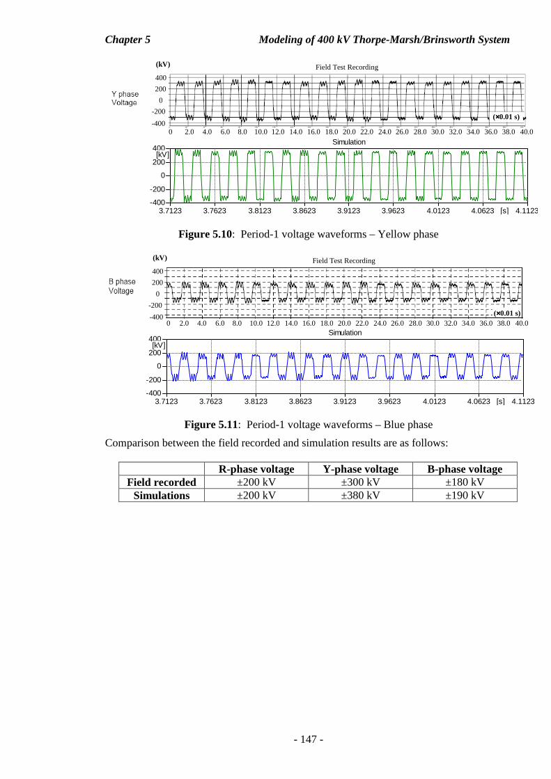
Chapter 5 Modeling of 400 kV Thorpe-Marsh/Brinsworth System
- 147 -
Figure 5.10: Period-1 voltage waveforms – Yellow phase
Figure 5.11: Period-1 voltage waveforms – Blue phase
Comparison between the field recorded and simulation results are as follows:
R-phase voltage Y-phase voltage B-phase voltage Field recorded ±200 kV ±300 kV ±180 kV
Simulations ±200 kV ±380 kV ±190 kV
3.7123 3.7623 3.8123 3.8623 3.9123 3.9623 4.0123 4.0623 4.1123[s]-400
-200
0
200
400[kV]
Simulation
Field Test Recording (kV)
200 400
-400
-200
0
(××××0.01 s)
0 2.0 4.0 6.0 8.0 10.0 12.0 14.0 16.0 18.0 20.0 22.0 24.0 26.0 28.0 30.0 32.0 34.0 36.0 38.0 40.0
0 2.0 4.0 6.0 8.0 10.0 12.0 14.0 16.0 18.0 20.0 22.0 24.0 26.0 28.0 30.0 32.0 34.0 36.0 38.0 40.0 (××××0.01 s)
Field Test Recording (kV)
200 400
-400
0
-200
3.7123 3.7623 3.8123 3.8623 3.9123 3.9623 4.0123 4.0623 4.1123[s]-400
-200
0
200
400[kV]
Simulation
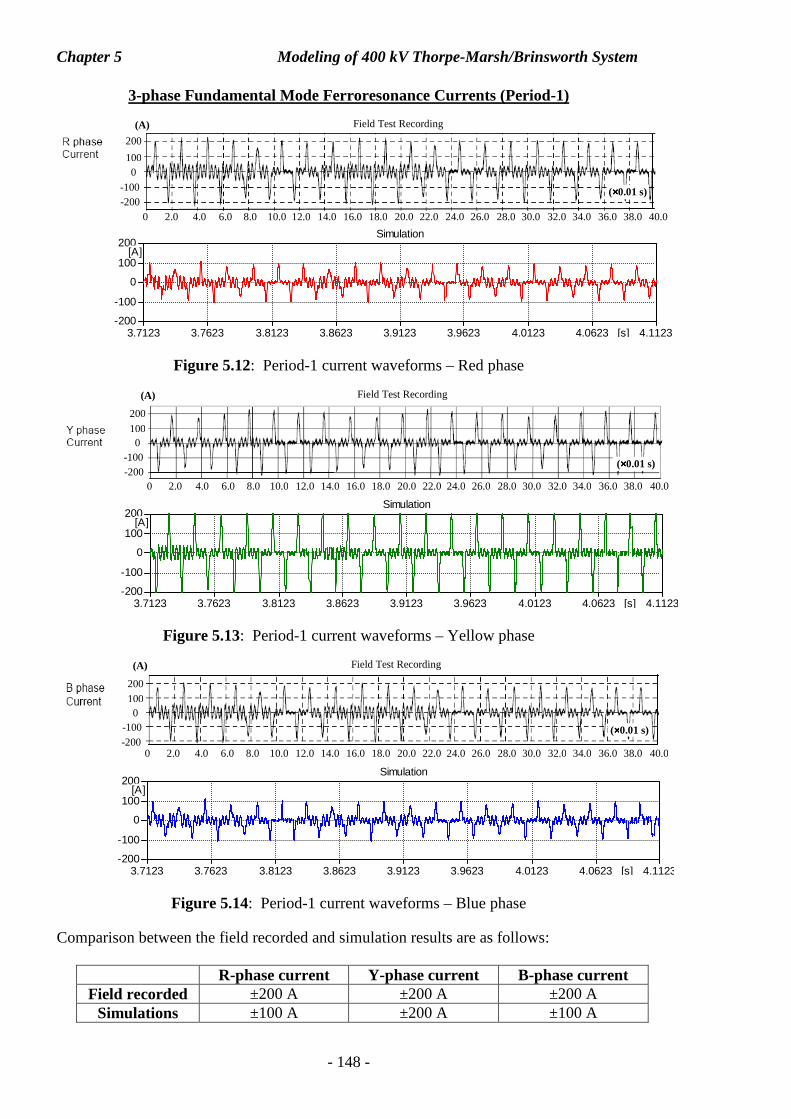
Chapter 5 Modeling of 400 kV Thorpe-Marsh/Brinsworth System
- 148 -
3-phase Fundamental Mode Ferroresonance Currents (Period-1)
Figure 5.12: Period-1 current waveforms – Red phase
Figure 5.13: Period-1 current waveforms – Yellow phase
Figure 5.14: Period-1 current waveforms – Blue phase
Comparison between the field recorded and simulation results are as follows:
R-phase current Y-phase current B-phase current Field recorded ±200 A ±200 A ±200 A
Simulations ±100 A ±200 A ±100 A
100 200
0
-200 -100
Field Test Recording (A)
0 2.0 4.0 6.0 8.0 10.0 12.0 14.0 16.0 18.0 20.0 22.0 24.0 26.0 28.0 30.0 32.0 34.0 36.0 38.0 40.0
(××××0.01 s)
3.7123 3.7623 3.8123 3.8623 3.9123 3.9623 4.0123 4.0623 4.1123[s]-200
-100
0
100
200[A]
Simulation
100 200
0
-200 -100
0 2.0 4.0 6.0 8.0 10.0 12.0 14.0 16.0 18.0 20.0 22.0 24.0 26.0 28.0 30.0 32.0 34.0 36.0 38.0 40.0
(××××0.01 s)
Field Test Recording (A)
3.7123 3.7623 3.8123 3.8623 3.9123 3.9623 4.0123 4.0623 4.1123[s]-200
-100
0
100
200[A]
Simulation
3.7123 3.7623 3.8123 3.8623 3.9123 3.9623 4.0123 4.0623 4.1123[s]-200
-100
0
100
200[A]
Simulation
0 2.0 4.0 6.0 8.0 10.0 12.0 14.0 16.0 18.0 20.0 22.0 24.0 26.0 28.0 30.0 32.0 34.0 36.0 38.0 40.0
100 200
0
-200 -100
Field Test Recording (A)
(××××0.01 s)
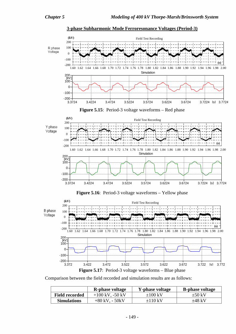
Chapter 5 Modeling of 400 kV Thorpe-Marsh/Brinsworth System
- 149 -
3-phase Subharmonic Mode Ferroresonance Voltages (Period-3)
Figure 5.15: Period-3 voltage waveforms – Red phase
Figure 5.16: Period-3 voltage waveforms – Yellow phase
Figure 5.17: Period-3 voltage waveforms – Blue phase
Comparison between the field recorded and simulation results are as follows:
R-phase voltage Y-phase voltage B-phase voltage Field recorded +100 kV, -50 kV ±100 kV ±50 kV
Simulations +80 kV, - 50kV ±110 kV ±48 kV
3.372 3.422 3.472 3.522 3.572 3.622 3.672 3.722 3.772[s]-200
-100
0
100
200[kV]
Simulation
3.3724 3.4224 3.4724 3.5224 3.5724 3.6224 3.6724 3.7224 3.7724[s]-200
-100
0
100
200[kV]
Simulation
3.3724 3.4224 3.4724 3.5224 3.5724 3.6224 3.6724 3.7224 3.7724[s]-200
-100
0
100
200[kV]
Simulation
(s)
Field Test Recording (kV)
100 200
0
-100
1.60 1.62 1.64 1.66 1.68 1.70 1.72 1.74 1.76 1.78 1.80 1.82 1.84 1.86 1.88 1.90 1.92 1.94 1.96 1.98 2.00 -200
(s)
Field Test Recording (kV)
100 200
-200
0
-100
1.60 1.62 1.64 1.66 1.68 1.70 1.72 1.74 1.76 1.78 1.80 1.82 1.84 1.86 1.88 1.90 1.92 1.94 1.96 1.98 2.00
(s)
Field Test Recording (kV)
100 200
0
-100
1.60 1.62 1.64 1.66 1.68 1.70 1.72 1.74 1.76 1.78 1.80 1.82 1.84 1.86 1.88 1.90 1.92 1.94 1.96 1.98 2.00 -200
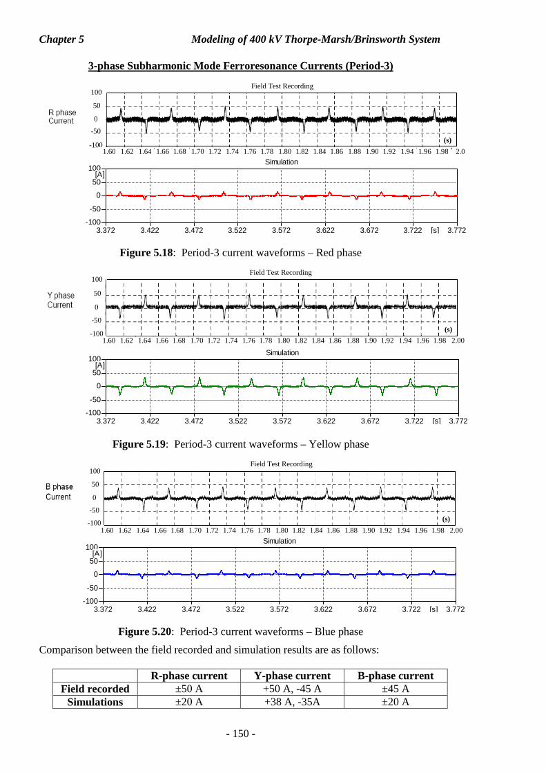
Chapter 5 Modeling of 400 kV Thorpe-Marsh/Brinsworth System
- 150 -
3-phase Subharmonic Mode Ferroresonance Currents (Period-3)
Figure 5.18: Period-3 current waveforms – Red phase
Figure 5.19: Period-3 current waveforms – Yellow phase
Figure 5.20: Period-3 current waveforms – Blue phase
Comparison between the field recorded and simulation results are as follows:
R-phase current Y-phase current B-phase current Field recorded ±50 A +50 A, -45 A ±45 A
Simulations ±20 A +38 A, -35A ±20 A
-50
50
100
-100
0
(s)
1.60 1.62 1.64 1.66 1.68 1.70 1.72 1.74 1.76 1.78 1.80 1.82 1.84 1.86 1.88 1.90 1.92 1.94 1.96 1.98 2.00
Field Test Recording
3.372 3.422 3.472 3.522 3.572 3.622 3.672 3.722 3.772[s]-100
-50
0
50
100[A]
Simulation
-50
50
100
-100
0
(s)
1.60 1.62 1.64 1.66 1.68 1.70 1.72 1.74 1.76 1.78 1.80 1.82 1.84 1.86 1.88 1.90 1.92 1.94 1.96 1.98 2.00
Field Test Recording
3.372 3.422 3.472 3.522 3.572 3.622 3.672 3.722 3.772[s]-100
-50
0
50
100[A]
Simulation
-50
50
100
-100
0
1.60 1.62 1.64 1.66 1.68 1.70 1.72 1.74 1.76 1.78 1.80 1.82 1.84 1.86 1.88 1.90 1.92 1.94 1.96 1.98 2.0
Field Test Recording
(s)
3.372 3.422 3.472 3.522 3.572 3.622 3.672 3.722 3.772[s]-100
-50
0
50
100[A]
Simulation
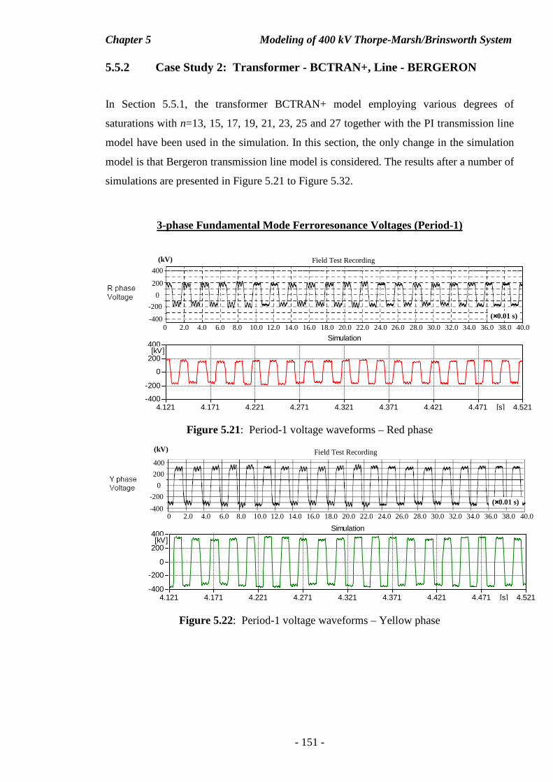
Chapter 5 Modeling of 400 kV Thorpe-Marsh/Brinsworth System
- 151 -
5.5.2 Case Study 2: Transformer - BCTRAN+, Line - BERGERON
In Section 5.5.1, the transformer BCTRAN+ model employing various degrees of
saturations with n=13, 15, 17, 19, 21, 23, 25 and 27 together with the PI transmission line
model have been used in the simulation. In this section, the only change in the simulation
model is that Bergeron transmission line model is considered. The results after a number of
simulations are presented in Figure 5.21 to Figure 5.32.
3-phase Fundamental Mode Ferroresonance Voltages (Period-1)
Figure 5.21: Period-1 voltage waveforms – Red phase
Figure 5.22: Period-1 voltage waveforms – Yellow phase
4.121 4.171 4.221 4.271 4.321 4.371 4.421 4.471 4.521[s]-400
-200
0
200
400[kV]
Simulation
4.121 4.171 4.221 4.271 4.321 4.371 4.421 4.471 4.521[s]-400
-200
0
200
400[kV]
Simulation
200 400
0
-400
-200
0 2.0 4.0 6.0 8.0 10.0 12.0 14.0 16.0 18.0 20.0 22.0 24.0 26.0 28.0 30.0 32.0 34.0 36.0 38.0 40.0
Field Test Recording (kV)
(××××0.01 s)
0 2.0 4.0 6.0 8.0 10.0 12.0 14.0 16.0 18.0 20.0 22.0 24.0 26.0 28.0 30.0 32.0 34.0 36.0 38.0 40.0
Field Test Recording (kV)
200 400
-400
-200
0
(××××0.01 s)
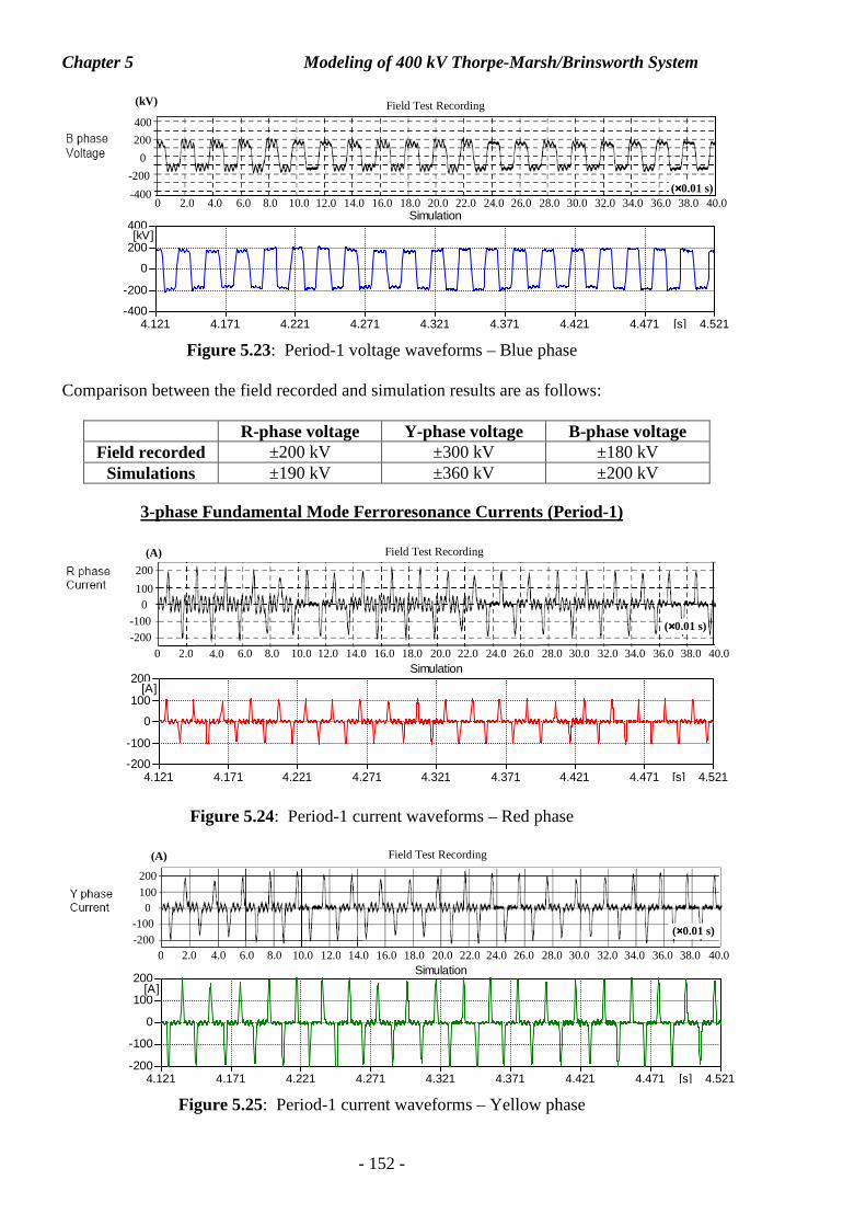
Chapter 5 Modeling of 400 kV Thorpe-Marsh/Brinsworth System
- 152 -
Figure 5.23: Period-1 voltage waveforms – Blue phase Comparison between the field recorded and simulation results are as follows:
R-phase voltage Y-phase voltage B-phase voltage Field recorded ±200 kV ±300 kV ±180 kV
Simulations ±190 kV ±360 kV ±200 kV
3-phase Fundamental Mode Ferroresonance Currents (Period-1)
Figure 5.24: Period-1 current waveforms – Red phase
Figure 5.25: Period-1 current waveforms – Yellow phase
100 200
0
-200 -100
0 2.0 4.0 6.0 8.0 10.0 12.0 14.0 16.0 18.0 20.0 22.0 24.0 26.0 28.0 30.0 32.0 34.0 36.0 38.0 40.0
(××××0.01 s)
Field Test Recording (A)
4.121 4.171 4.221 4.271 4.321 4.371 4.421 4.471 4.521[s]-200
-100
0
100
200[A]
Simulation
4.121 4.171 4.221 4.271 4.321 4.371 4.421 4.471 4.521[s]-200
-100
0
100
200[A]
Simulation
4.121 4.171 4.221 4.271 4.321 4.371 4.421 4.471 4.521[s]-400
-200
0
200
400[kV]
Simulation0 2.0 4.0 6.0 8.0 10.0 12.0 14.0 16.0 18.0 20.0 22.0 24.0 26.0 28.0 30.0 32.0 34.0 36.0 38.0 40.0
(××××0.01 s)
Field Test Recording (kV)
200 400
-400
0
-200
0 2.0 4.0 6.0 8.0 10.0 12.0 14.0 16.0 18.0 20.0 22.0 24.0 26.0 28.0 30.0 32.0 34.0 36.0 38.0 40.0
100 200
0
-200 -100
Field Test Recording (A)
(××××0.01 s)
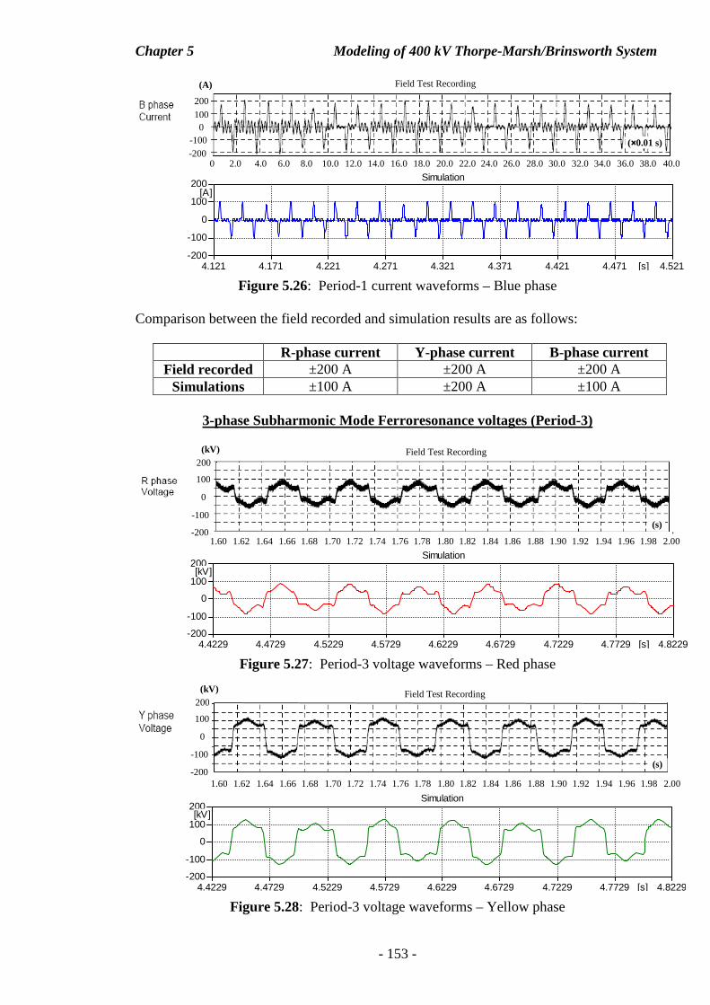
Chapter 5 Modeling of 400 kV Thorpe-Marsh/Brinsworth System
- 153 -
Figure 5.26: Period-1 current waveforms – Blue phase
Comparison between the field recorded and simulation results are as follows:
R-phase current Y-phase current B-phase current
Field recorded ±200 A ±200 A ±200 A Simulations ±100 A ±200 A ±100 A
3-phase Subharmonic Mode Ferroresonance voltages (Period-3)
Figure 5.27: Period-3 voltage waveforms – Red phase
Figure 5.28: Period-3 voltage waveforms – Yellow phase
4.4229 4.4729 4.5229 4.5729 4.6229 4.6729 4.7229 4.7729 4.8229[s]-200
-100
0
100
200[kV]
Simulation
4.4229 4.4729 4.5229 4.5729 4.6229 4.6729 4.7229 4.7729 4.8229[s]-200
-100
0
100
200[kV]
Simulation
100 200
0
-200 -100
Field Test Recording (A)
0 2.0 4.0 6.0 8.0 10.0 12.0 14.0 16.0 18.0 20.0 22.0 24.0 26.0 28.0 30.0 32.0 34.0 36.0 38.0 40.0
(××××0.01 s)
4.121 4.171 4.221 4.271 4.321 4.371 4.421 4.471 4.521[s]-200
-100
0
100
200[A]
Simulation
(s)
Field Test Recording (kV)
100 200
0
-100
-200 1.60 1.62 1.64 1.66 1.68 1.70 1.72 1.74 1.76 1.78 1.80 1.82 1.84 1.86 1.88 1.90 1.92 1.94 1.96 1.98 2.00
(s)
Field Test Recording (kV)
100 200
-200
0
-100
1.60 1.62 1.64 1.66 1.68 1.70 1.72 1.74 1.76 1.78 1.80 1.82 1.84 1.86 1.88 1.90 1.92 1.94 1.96 1.98 2.00
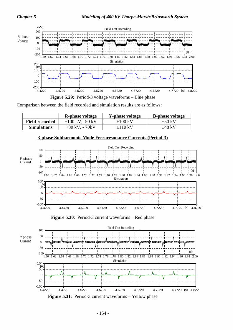
Chapter 5 Modeling of 400 kV Thorpe-Marsh/Brinsworth System
- 154 -
Figure 5.29: Period-3 voltage waveforms – Blue phase
Comparison between the field recorded and simulation results are as follows:
R-phase voltage Y-phase voltage B-phase voltage Field recorded +100 kV, -50 kV ±100 kV ±50 kV
Simulations +80 kV, - 70kV ±110 kV ±48 kV
3-phase Subharmonic Mode Ferroresonance Currents (Period-3)
Figure 5.30: Period-3 current waveforms – Red phase
Figure 5.31: Period-3 current waveforms – Yellow phase
-50
50
100
-100
0
(s)
1.60 1.62 1.64 1.66 1.68 1.70 1.72 1.74 1.76 1.78 1.80 1.82 1.84 1.86 1.88 1.90 1.92 1.94 1.96 1.98 2.00
Field Test Recording
4.4229 4.4729 4.5229 4.5729 4.6229 4.6729 4.7229 4.7729 4.8229[s]-100
-50
0
50
100[A]
Simulation
-50
50
100
-100
0
1.60 1.62 1.64 1.66 1.68 1.70 1.72 1.74 1.76 1.78 1.80 1.82 1.84 1.86 1.88 1.90 1.92 1.94 1.96 1.98 2.0
Field Test Recording
(s)
4.4229 4.4729 4.5229 4.5729 4.6229 4.6729 4.7229 4.7729 4.8229[s]-100
-50
0
50
100[A]
Simulation
(s)
Field Test Recording (kV)
100 200
0
-100
1.60 1.62 1.64 1.66 1.68 1.70 1.72 1.74 1.76 1.78 1.80 1.82 1.84 1.86 1.88 1.90 1.92 1.94 1.96 1.98 2.00 -200
4.4229 4.4729 4.5229 4.5729 4.6229 4.6729 4.7229 4.7729 4.8229[s]-200
-100
0
100
200[kV]
Simulation
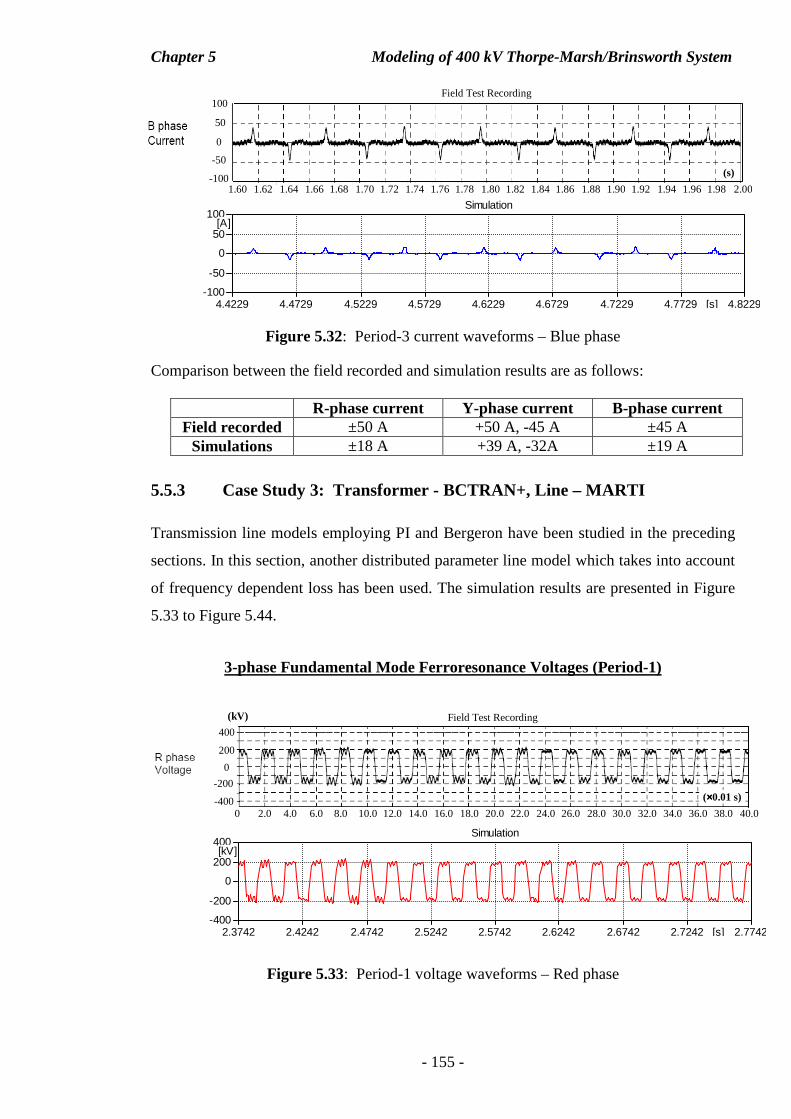
Chapter 5 Modeling of 400 kV Thorpe-Marsh/Brinsworth System
- 155 -
Figure 5.32: Period-3 current waveforms – Blue phase
Comparison between the field recorded and simulation results are as follows:
R-phase current Y-phase current B-phase current Field recorded ±50 A +50 A, -45 A ±45 A
Simulations ±18 A +39 A, -32A ±19 A
5.5.3 Case Study 3: Transformer - BCTRAN+, Line – MARTI
Transmission line models employing PI and Bergeron have been studied in the preceding
sections. In this section, another distributed parameter line model which takes into account
of frequency dependent loss has been used. The simulation results are presented in Figure
5.33 to Figure 5.44.
3-phase Fundamental Mode Ferroresonance Voltages (Period-1)
Figure 5.33: Period-1 voltage waveforms – Red phase
200 400
0
-400
-200
0 2.0 4.0 6.0 8.0 10.0 12.0 14.0 16.0 18.0 20.0 22.0 24.0 26.0 28.0 30.0 32.0 34.0 36.0 38.0 40.0
Field Test Recording (kV)
(××××0.01 s)
2.3742 2.4242 2.4742 2.5242 2.5742 2.6242 2.6742 2.7242 2.7742[s]-400
-200
0
200
400[kV]
Simulation
4.4229 4.4729 4.5229 4.5729 4.6229 4.6729 4.7229 4.7729 4.8229[s]-100
-50
0
50
100[A]
Simulation
-50
50
100
-100
0
(s)
1.60 1.62 1.64 1.66 1.68 1.70 1.72 1.74 1.76 1.78 1.80 1.82 1.84 1.86 1.88 1.90 1.92 1.94 1.96 1.98 2.00
Field Test Recording
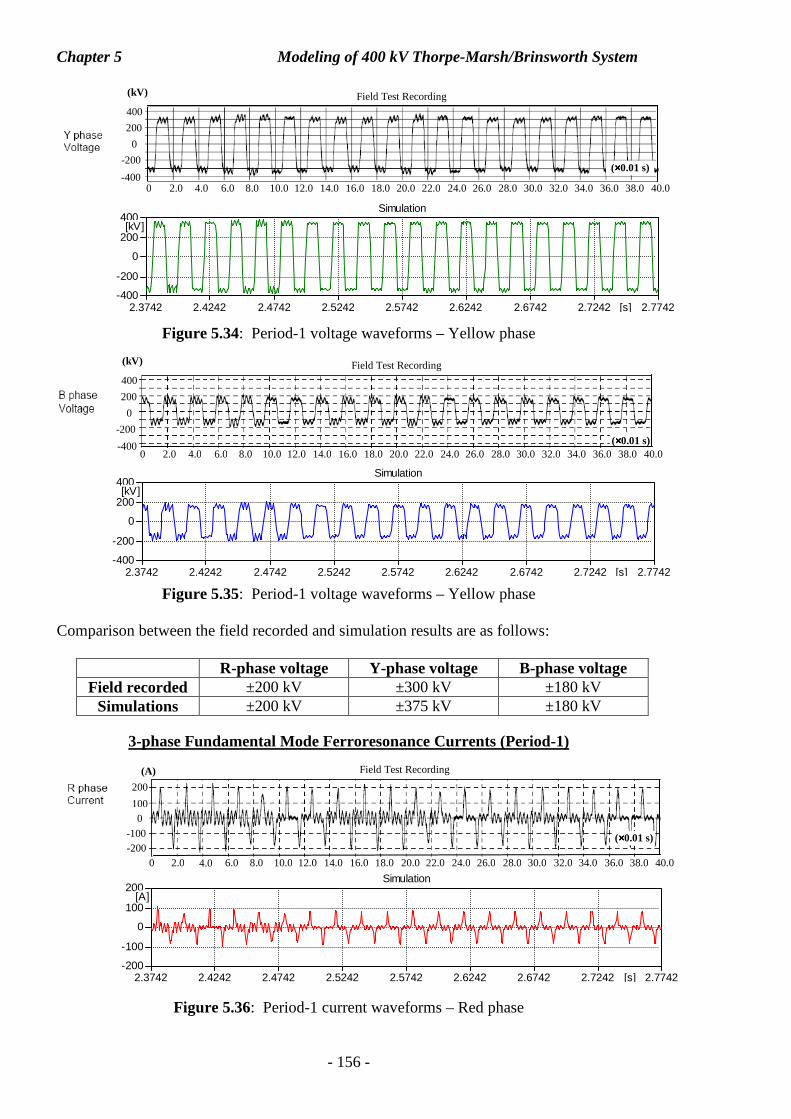
Chapter 5 Modeling of 400 kV Thorpe-Marsh/Brinsworth System
- 156 -
Figure 5.34: Period-1 voltage waveforms – Yellow phase
Figure 5.35: Period-1 voltage waveforms – Yellow phase Comparison between the field recorded and simulation results are as follows:
R-phase voltage Y-phase voltage B-phase voltage Field recorded ±200 kV ±300 kV ±180 kV
Simulations ±200 kV ±375 kV ±180 kV
3-phase Fundamental Mode Ferroresonance Currents (Period-1)
Figure 5.36: Period-1 current waveforms – Red phase
0 2.0 4.0 6.0 8.0 10.0 12.0 14.0 16.0 18.0 20.0 22.0 24.0 26.0 28.0 30.0 32.0 34.0 36.0 38.0 40.0
100 200
0
-200 -100
Field Test Recording (A)
(××××0.01 s)
2.3742 2.4242 2.4742 2.5242 2.5742 2.6242 2.6742 2.7242 2.7742[s]-200
-100
0
100
200[A]
Simulation
2.3742 2.4242 2.4742 2.5242 2.5742 2.6242 2.6742 2.7242 2.7742[s]-400
-200
0
200
400[kV]
Simulation
0 2.0 4.0 6.0 8.0 10.0 12.0 14.0 16.0 18.0 20.0 22.0 24.0 26.0 28.0 30.0 32.0 34.0 36.0 38.0 40.0
Field Test Recording (kV)
200 400
-400
-200
0
(××××0.01 s)
2.3742 2.4242 2.4742 2.5242 2.5742 2.6242 2.6742 2.7242 2.7742[s]-400
-200
0
200
400[kV]
Simulation
0 2.0 4.0 6.0 8.0 10.0 12.0 14.0 16.0 18.0 20.0 22.0 24.0 26.0 28.0 30.0 32.0 34.0 36.0 38.0 40.0 (××××0.01 s)
Field Test Recording (kV)
200 400
-400
0
-200
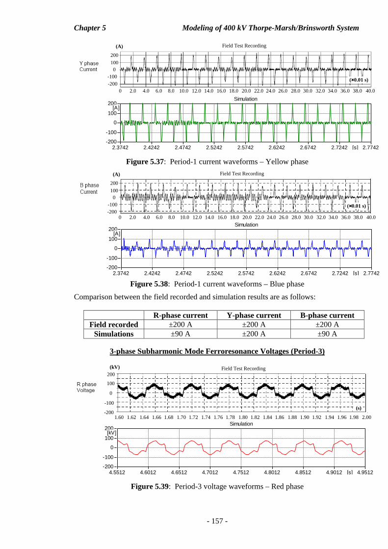
Chapter 5 Modeling of 400 kV Thorpe-Marsh/Brinsworth System
- 157 -
Figure 5.37: Period-1 current waveforms – Yellow phase
Figure 5.38: Period-1 current waveforms – Blue phase
Comparison between the field recorded and simulation results are as follows:
R-phase current Y-phase current B-phase current Field recorded ±200 A ±200 A ±200 A
Simulations ±90 A ±200 A ±90 A
3-phase Subharmonic Mode Ferroresonance Voltages (Period-3)
Figure 5.39: Period-3 voltage waveforms – Red phase
4.5512 4.6012 4.6512 4.7012 4.7512 4.8012 4.8512 4.9012 4.9512[s]-200
-100
0
100
200[kV]
Simulation
100 200
0
-200 -100
Field Test Recording (A)
0 2.0 4.0 6.0 8.0 10.0 12.0 14.0 16.0 18.0 20.0 22.0 24.0 26.0 28.0 30.0 32.0 34.0 36.0 38.0 40.0
(××××0.01 s)
2.3742 2.4242 2.4742 2.5242 2.5742 2.6242 2.6742 2.7242 2.7742[s]-200
-100
0
100
200[A]
Simulation
100 200
0
-200 -100
0 2.0 4.0 6.0 8.0 10.0 12.0 14.0 16.0 18.0 20.0 22.0 24.0 26.0 28.0 30.0 32.0 34.0 36.0 38.0 40.0
(××××0.01 s)
Field Test Recording (A)
2.3742 2.4242 2.4742 2.5242 2.5742 2.6242 2.6742 2.7242 2.7742[s]-200
-100
0
100
200[A]
Simulation
(s)
Field Test Recording (kV)
100 200
0
-100
-200 1.60 1.62 1.64 1.66 1.68 1.70 1.72 1.74 1.76 1.78 1.80 1.82 1.84 1.86 1.88 1.90 1.92 1.94 1.96 1.98 2.00
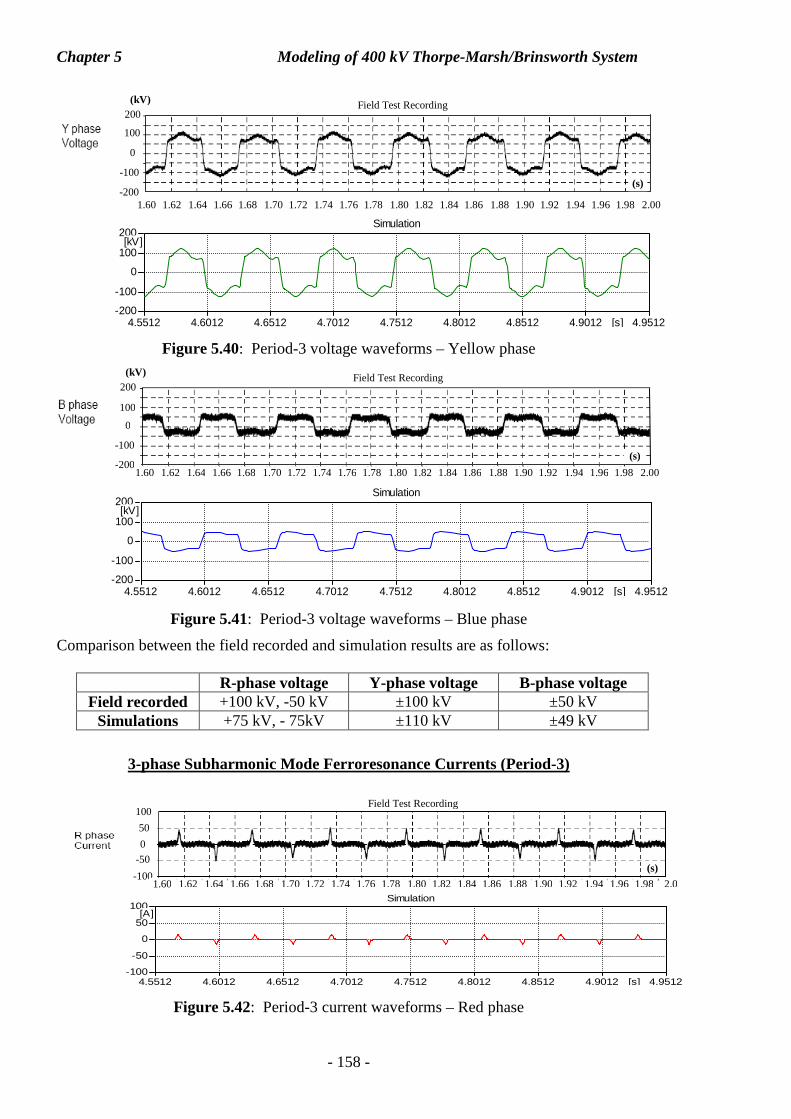
Chapter 5 Modeling of 400 kV Thorpe-Marsh/Brinsworth System
- 158 -
Figure 5.40: Period-3 voltage waveforms – Yellow phase
Figure 5.41: Period-3 voltage waveforms – Blue phase
Comparison between the field recorded and simulation results are as follows:
R-phase voltage Y-phase voltage B-phase voltage Field recorded +100 kV, -50 kV ±100 kV ±50 kV
Simulations +75 kV, - 75kV ±110 kV ±49 kV
3-phase Subharmonic Mode Ferroresonance Currents (Period-3)
Figure 5.42: Period-3 current waveforms – Red phase
-50
50
100
-100
0
1.60 1.62 1.64 1.66 1.68 1.70 1.72 1.74 1.76 1.78 1.80 1.82 1.84 1.86 1.88 1.90 1.92 1.94 1.96 1.98 2.0
(s)
Field Test Recording
4.5512 4.6012 4.6512 4.7012 4.7512 4.8012 4.8512 4.9012 4.9512[s]-100
-50
0
50
100[A]
Simulation
4.5512 4.6012 4.6512 4.7012 4.7512 4.8012 4.8512 4.9012 4.9512[s]-200
-100
0
100
200[kV]
Simulation
(s)
Field Test Recording (kV)
100 200
-200
0
-100
1.60 1.62 1.64 1.66 1.68 1.70 1.72 1.74 1.76 1.78 1.80 1.82 1.84 1.86 1.88 1.90 1.92 1.94 1.96 1.98 2.00
4.5512 4.6012 4.6512 4.7012 4.7512 4.8012 4.8512 4.9012 4.9512[s]-200
-100
0
100
200[kV]
Simulation
(s)
Field Test Recording (kV)
100 200
0
-100
1.60 1.62 1.64 1.66 1.68 1.70 1.72 1.74 1.76 1.78 1.80 1.82 1.84 1.86 1.88 1.90 1.92 1.94 1.96 1.98 2.00 -200
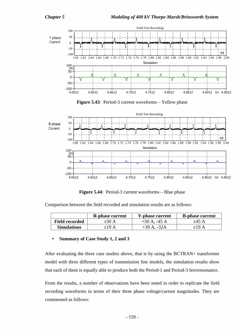
Chapter 5 Modeling of 400 kV Thorpe-Marsh/Brinsworth System
- 159 -
Figure 5.43: Period-3 current waveforms – Yellow phase
Figure 5.44: Period-3 current waveforms – Blue phase
Comparison between the field recorded and simulation results are as follows:
R-phase current Y-phase current B-phase current Field recorded ±50 A +50 A, -45 A ±45 A
Simulations ±19 A +39 A, -32A ±19 A
• Summary of Case Study 1, 2 and 3
After evaluating the three case studies above, that is by using the BCTRAN+ transformer
model with three different types of transmission line models, the simulation results show
that each of them is equally able to produce both the Period-1 and Period-3 ferroresonance.
From the results, a number of observations have been noted in order to replicate the field
recording waveforms in terms of their three phase voltage/current magnitudes. They are
commented as follows:
-50
50
100
-100
0
(s)
1.60 1.62 1.64 1.66 1.68 1.70 1.72 1.74 1.76 1.78 1.80 1.82 1.84 1.86 1.88 1.90 1.92 1.94 1.96 1.98 2.00
Field Test Recording
4.5512 4.6012 4.6512 4.7012 4.7512 4.8012 4.8512 4.9012 4.9512[s]-100
-50
0
50
100[A]
Simulation
-50
50
100
-100
0
(s)
1.60 1.62 1.64 1.66 1.68 1.70 1.72 1.74 1.76 1.78 1.80 1.82 1.84 1.86 1.88 1.90 1.92 1.94 1.96 1.98 2.00
Field Test Recording
4.5512 4.6012 4.6512 4.7012 4.7512 4.8012 4.8512 4.9012 4.9512[s]-100
-50
0
50
100[A]
Simulation
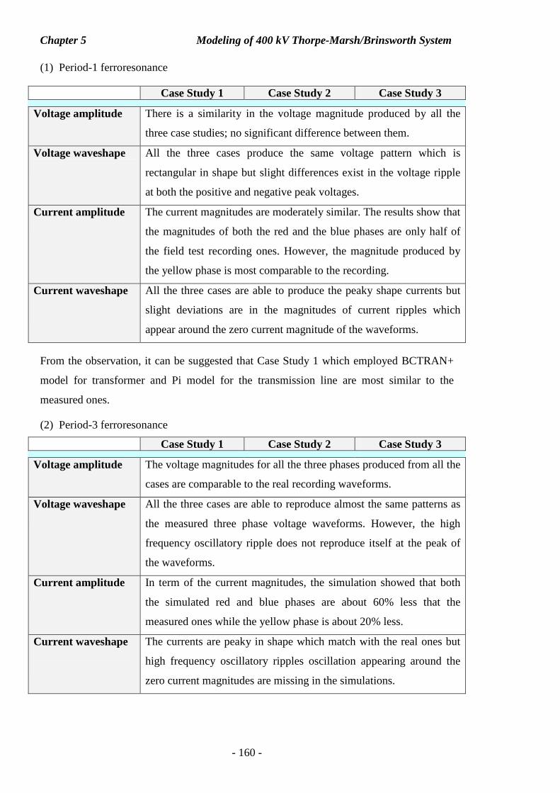
Chapter 5 Modeling of 400 kV Thorpe-Marsh/Brinsworth System
- 160 -
(1) Period-1 ferroresonance
Case Study 1 Case Study 2 Case Study 3
Voltage amplitude There is a similarity in the voltage magnitude produced by all the
three case studies; no significant difference between them.
Voltage waveshape
All the three cases produce the same voltage pattern which is
rectangular in shape but slight differences exist in the voltage ripple
at both the positive and negative peak voltages.
Current amplitude
The current magnitudes are moderately similar. The results show that
the magnitudes of both the red and the blue phases are only half of
the field test recording ones. However, the magnitude produced by
the yellow phase is most comparable to the recording.
Current waveshape
All the three cases are able to produce the peaky shape currents but
slight deviations are in the magnitudes of current ripples which
appear around the zero current magnitude of the waveforms.
From the observation, it can be suggested that Case Study 1 which employed BCTRAN+
model for transformer and Pi model for the transmission line are most similar to the
measured ones.
(2) Period-3 ferroresonance
Case Study 1 Case Study 2 Case Study 3
Voltage amplitude The voltage magnitudes for all the three phases produced from all the
cases are comparable to the real recording waveforms.
Voltage waveshape
All the three cases are able to reproduce almost the same patterns as
the measured three phase voltage waveforms. However, the high
frequency oscillatory ripple does not reproduce itself at the peak of
the waveforms.
Current amplitude
In term of the current magnitudes, the simulation showed that both
the simulated red and blue phases are about 60% less that the
measured ones while the yellow phase is about 20% less.
Current waveshape
The currents are peaky in shape which match with the real ones but
high frequency oscillatory ripples oscillation appearing around the
zero current magnitudes are missing in the simulations.
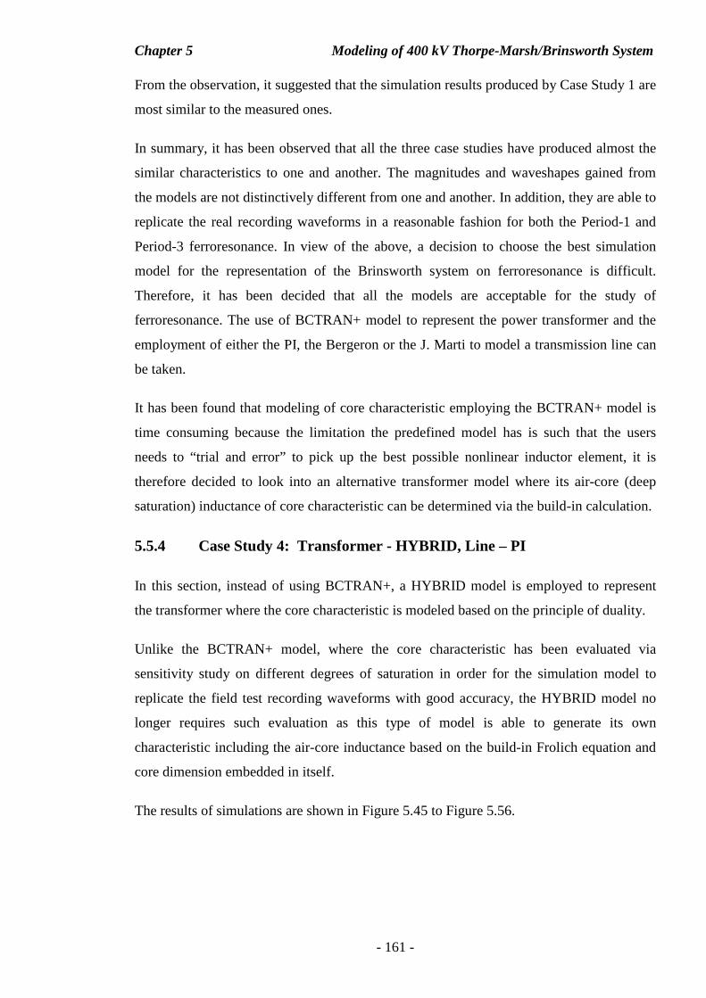
Chapter 5 Modeling of 400 kV Thorpe-Marsh/Brinsworth System
- 161 -
From the observation, it suggested that the simulation results produced by Case Study 1 are
most similar to the measured ones.
In summary, it has been observed that all the three case studies have produced almost the
similar characteristics to one and another. The magnitudes and waveshapes gained from
the models are not distinctively different from one and another. In addition, they are able to
replicate the real recording waveforms in a reasonable fashion for both the Period-1 and
Period-3 ferroresonance. In view of the above, a decision to choose the best simulation
model for the representation of the Brinsworth system on ferroresonance is difficult.
Therefore, it has been decided that all the models are acceptable for the study of
ferroresonance. The use of BCTRAN+ model to represent the power transformer and the
employment of either the PI, the Bergeron or the J. Marti to model a transmission line can
be taken.
It has been found that modeling of core characteristic employing the BCTRAN+ model is
time consuming because the limitation the predefined model has is such that the users
needs to “trial and error” to pick up the best possible nonlinear inductor element, it is
therefore decided to look into an alternative transformer model where its air-core (deep
saturation) inductance of core characteristic can be determined via the build-in calculation.
5.5.4 Case Study 4: Transformer - HYBRID, Line – PI
In this section, instead of using BCTRAN+, a HYBRID model is employed to represent
the transformer where the core characteristic is modeled based on the principle of duality.
Unlike the BCTRAN+ model, where the core characteristic has been evaluated via
sensitivity study on different degrees of saturation in order for the simulation model to
replicate the field test recording waveforms with good accuracy, the HYBRID model no
longer requires such evaluation as this type of model is able to generate its own
characteristic including the air-core inductance based on the build-in Frolich equation and
core dimension embedded in itself.
The results of simulations are shown in Figure 5.45 to Figure 5.56.
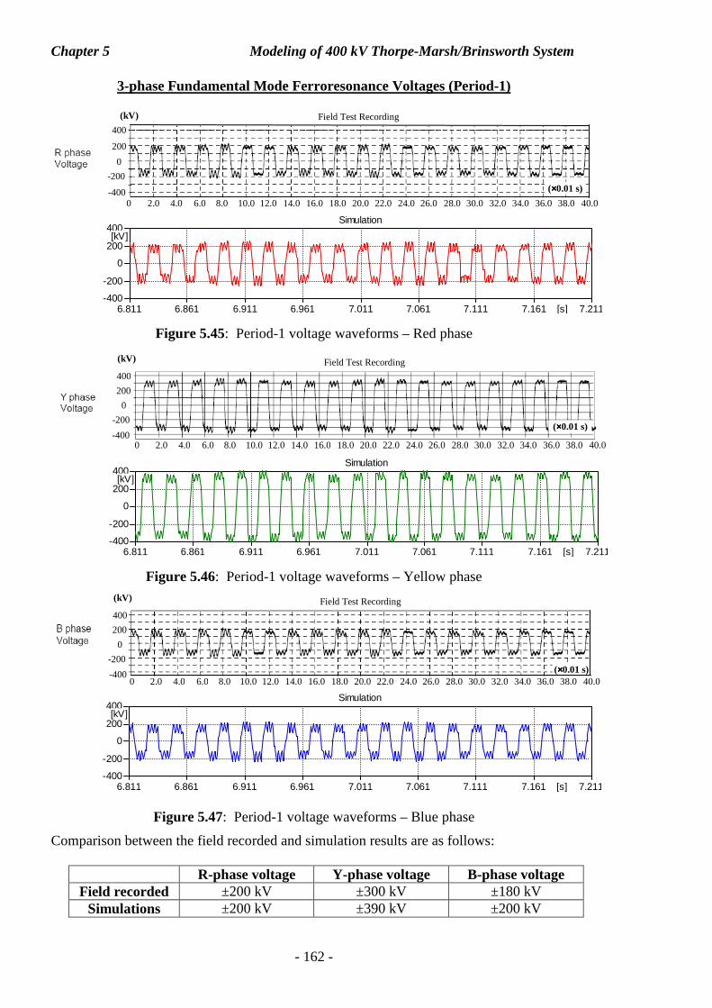
Chapter 5 Modeling of 400 kV Thorpe-Marsh/Brinsworth System
- 162 -
3-phase Fundamental Mode Ferroresonance Voltages (Period-1)
Figure 5.45: Period-1 voltage waveforms – Red phase
Figure 5.46: Period-1 voltage waveforms – Yellow phase
Figure 5.47: Period-1 voltage waveforms – Blue phase
Comparison between the field recorded and simulation results are as follows:
R-phase voltage Y-phase voltage B-phase voltage Field recorded ±200 kV ±300 kV ±180 kV
Simulations ±200 kV ±390 kV ±200 kV
0 2.0 4.0 6.0 8.0 10.0 12.0 14.0 16.0 18.0 20.0 22.0 24.0 26.0 28.0 30.0 32.0 34.0 36.0 38.0 40.0
Field Test Recording (kV)
200 400
-400
-200
0
(××××0.01 s)
6.811 6.861 6.911 6.961 7.011 7.061 7.111 7.161 7.211[s]-400
-200
0
200
400[kV]
Simulation
0 2.0 4.0 6.0 8.0 10.0 12.0 14.0 16.0 18.0 20.0 22.0 24.0 26.0 28.0 30.0 32.0 34.0 36.0 38.0 40.0 (××××0.01 s)
Field Test Recording (kV)
200 400
-400
0
-200
6.811 6.861 6.911 6.961 7.011 7.061 7.111 7.161 7.211[s]-400
-200
0
200
400[kV]
Simulation
200 400
0
-400
-200
0 2.0 4.0 6.0 8.0 10.0 12.0 14.0 16.0 18.0 20.0 22.0 24.0 26.0 28.0 30.0 32.0 34.0 36.0 38.0 40.0
Field Test Recording (kV)
(××××0.01 s)
6.811 6.861 6.911 6.961 7.011 7.061 7.111 7.161 7.211[s]-400
-200
0
200
400[kV]
Simulation
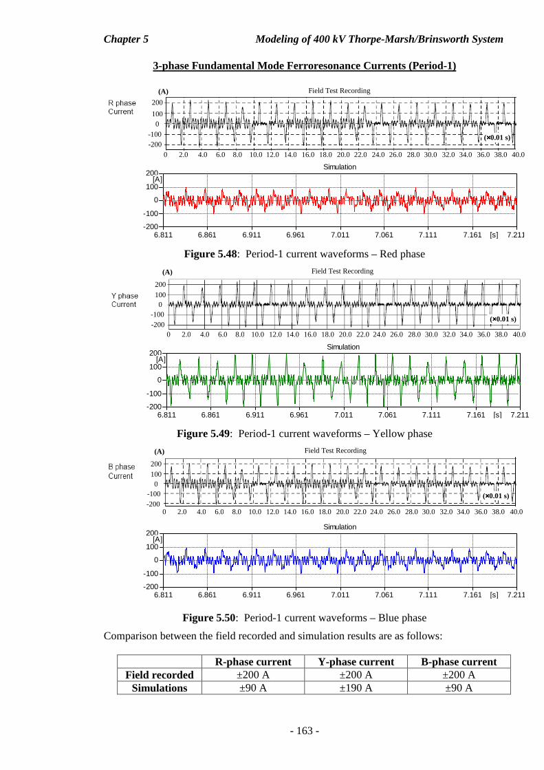
Chapter 5 Modeling of 400 kV Thorpe-Marsh/Brinsworth System
- 163 -
3-phase Fundamental Mode Ferroresonance Currents (Period-1)
Figure 5.48: Period-1 current waveforms – Red phase
Figure 5.49: Period-1 current waveforms – Yellow phase
Figure 5.50: Period-1 current waveforms – Blue phase
Comparison between the field recorded and simulation results are as follows:
R-phase current Y-phase current B-phase current Field recorded ±200 A ±200 A ±200 A
Simulations ±90 A ±190 A ±90 A
100 200
0
-200 -100
Field Test Recording (A)
0 2.0 4.0 6.0 8.0 10.0 12.0 14.0 16.0 18.0 20.0 22.0 24.0 26.0 28.0 30.0 32.0 34.0 36.0 38.0 40.0
(××××0.01 s)
6.811 6.861 6.911 6.961 7.011 7.061 7.111 7.161 7.211[s]-200
-100
0
100
200[A]
Simulation
100 200
0
-200 -100
0 2.0 4.0 6.0 8.0 10.0 12.0 14.0 16.0 18.0 20.0 22.0 24.0 26.0 28.0 30.0 32.0 34.0 36.0 38.0 40.0
(××××0.01 s)
Field Test Recording (A)
6.811 6.861 6.911 6.961 7.011 7.061 7.111 7.161 7.211[s]-200
-100
0
100
200[A]
Simulation
0 2.0 4.0 6.0 8.0 10.0 12.0 14.0 16.0 18.0 20.0 22.0 24.0 26.0 28.0 30.0 32.0 34.0 36.0 38.0 40.0
100 200
0
-200 -100
Field Test Recording (A)
(××××0.01 s)
6.811 6.861 6.911 6.961 7.011 7.061 7.111 7.161 7.211[s]-200
-100
0
100
200[A]
Simulation
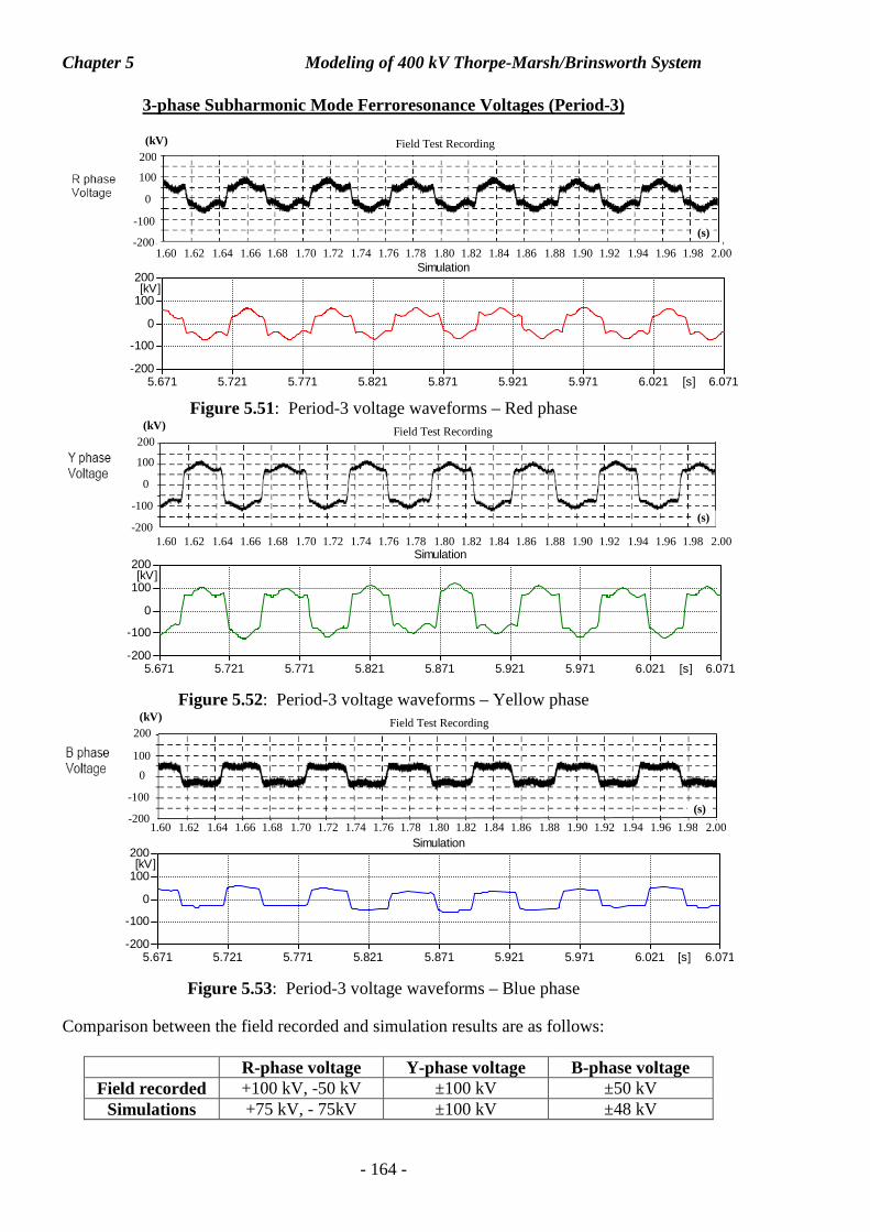
Chapter 5 Modeling of 400 kV Thorpe-Marsh/Brinsworth System
- 164 -
3-phase Subharmonic Mode Ferroresonance Voltages (Period-3)
Figure 5.51: Period-3 voltage waveforms – Red phase
Figure 5.52: Period-3 voltage waveforms – Yellow phase
Figure 5.53: Period-3 voltage waveforms – Blue phase
Comparison between the field recorded and simulation results are as follows:
R-phase voltage Y-phase voltage B-phase voltage Field recorded +100 kV, -50 kV ±100 kV ±50 kV
Simulations +75 kV, - 75kV ±100 kV ±48 kV
(s)
Field Test Recording (kV)
100 200
0
-100
1.60 1.62 1.64 1.66 1.68 1.70 1.72 1.74 1.76 1.78 1.80 1.82 1.84 1.86 1.88 1.90 1.92 1.94 1.96 1.98 2.00 -200
5.671 5.721 5.771 5.821 5.871 5.921 5.971 6.021 6.071[s]-200
-100
0
100
200[kV]
Simulation
(s)
Field Test Recording (kV)
100 200
-200
0
-100
1.60 1.62 1.64 1.66 1.68 1.70 1.72 1.74 1.76 1.78 1.80 1.82 1.84 1.86 1.88 1.90 1.92 1.94 1.96 1.98 2.00
5.671 5.721 5.771 5.821 5.871 5.921 5.971 6.021 6.071[s]-200
-100
0
100
200[kV]
Simulation
(s)
Field Test Recording (kV)
100 200
0
-100
-200 1.60 1.62 1.64 1.66 1.68 1.70 1.72 1.74 1.76 1.78 1.80 1.82 1.84 1.86 1.88 1.90 1.92 1.94 1.96 1.98 2.00
5.671 5.721 5.771 5.821 5.871 5.921 5.971 6.021 6.071[s]-200
-100
0
100
200[kV]
Simulation
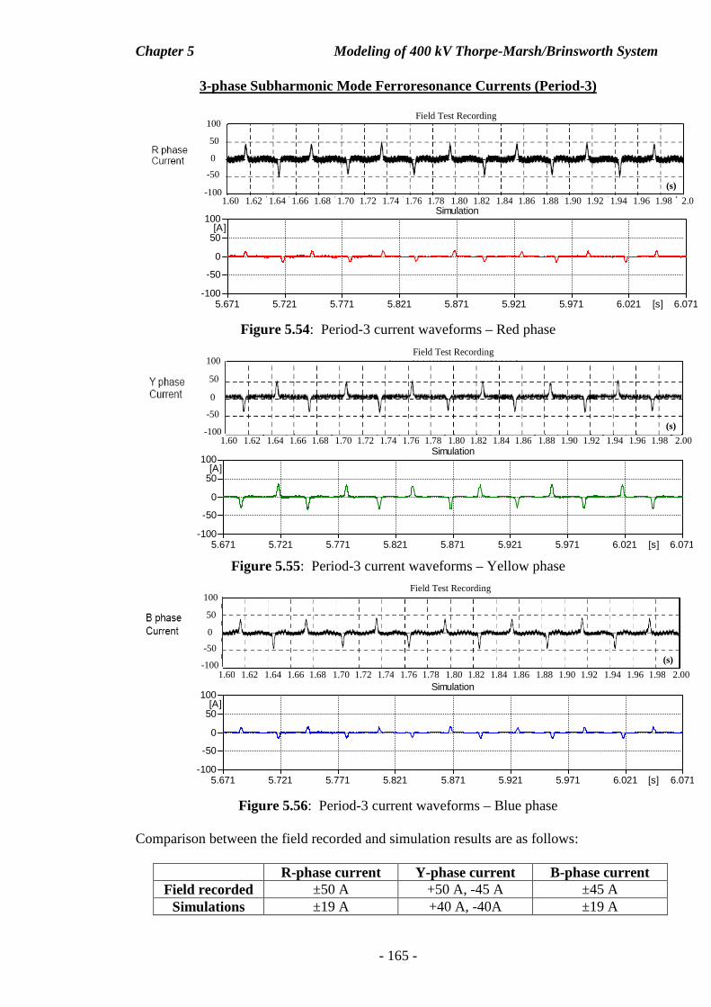
Chapter 5 Modeling of 400 kV Thorpe-Marsh/Brinsworth System
- 165 -
3-phase Subharmonic Mode Ferroresonance Currents (Period-3)
Figure 5.54: Period-3 current waveforms – Red phase
Figure 5.55: Period-3 current waveforms – Yellow phase
Figure 5.56: Period-3 current waveforms – Blue phase
Comparison between the field recorded and simulation results are as follows:
R-phase current Y-phase current B-phase current Field recorded ±50 A +50 A, -45 A ±45 A
Simulations ±19 A +40 A, -40A ±19 A
-50
50
100
-100
0
(s)
1.60 1.62 1.64 1.66 1.68 1.70 1.72 1.74 1.76 1.78 1.80 1.82 1.84 1.86 1.88 1.90 1.92 1.94 1.96 1.98 2.00
Field Test Recording
5.671 5.721 5.771 5.821 5.871 5.921 5.971 6.021 6.071[s]-100
-50
0
50
100[A]
Simulation
-50
50
100
-100
0
(s)
1.60 1.62 1.64 1.66 1.68 1.70 1.72 1.74 1.76 1.78 1.80 1.82 1.84 1.86 1.88 1.90 1.92 1.94 1.96 1.98 2.00
Field Test Recording
5.671 5.721 5.771 5.821 5.871 5.921 5.971 6.021 6.071[s]-100
-50
0
50
100[A]
Simulation
-50
50
100
-100
0
1.60 1.62 1.64 1.66 1.68 1.70 1.72 1.74 1.76 1.78 1.80 1.82 1.84 1.86 1.88 1.90 1.92 1.94 1.96 1.98 2.0
Field Test Recording
(s)
5.671 5.721 5.771 5.821 5.871 5.921 5.971 6.021 6.071[s]-100
-50
0
50
100[A]
Simulation
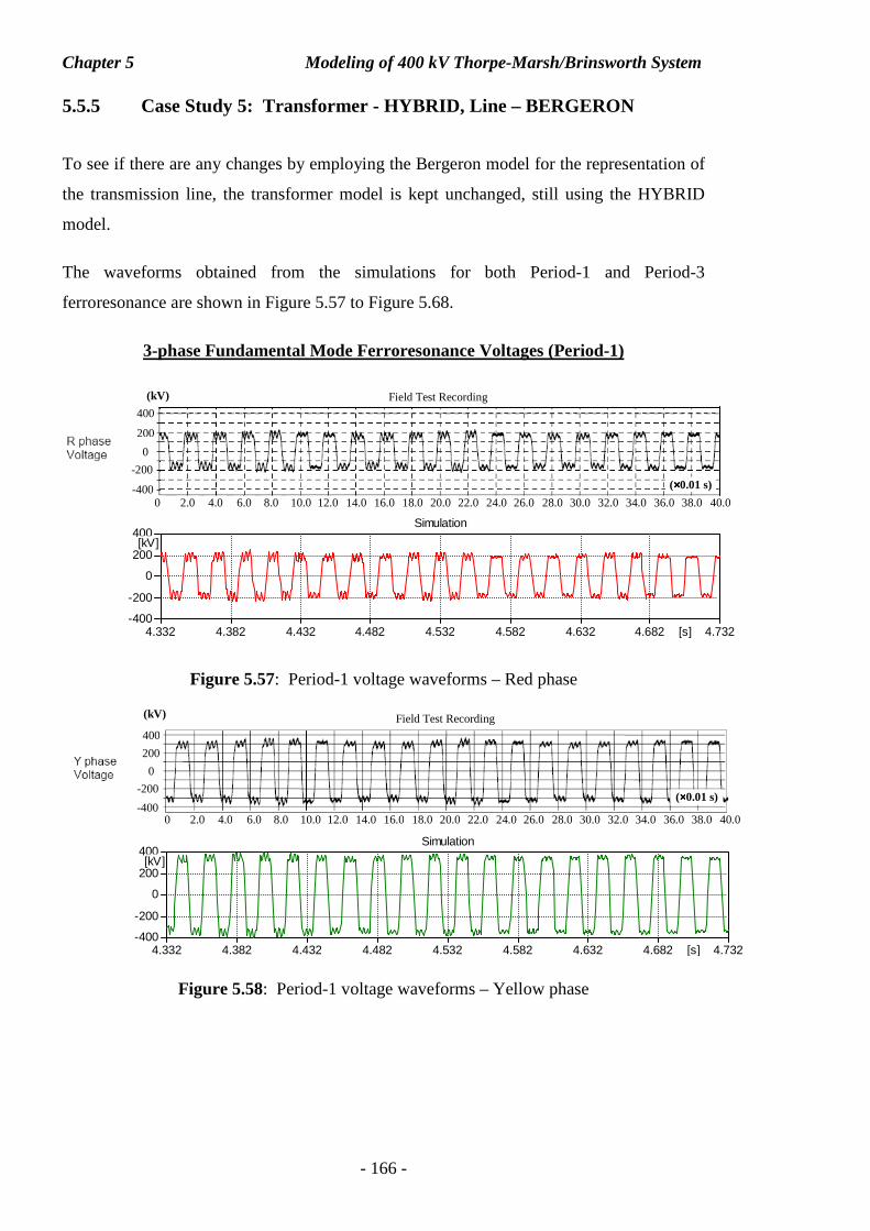
Chapter 5 Modeling of 400 kV Thorpe-Marsh/Brinsworth System
- 166 -
5.5.5 Case Study 5: Transformer - HYBRID, Line – BERGERON
To see if there are any changes by employing the Bergeron model for the representation of
the transmission line, the transformer model is kept unchanged, still using the HYBRID
model.
The waveforms obtained from the simulations for both Period-1 and Period-3
ferroresonance are shown in Figure 5.57 to Figure 5.68.
3-phase Fundamental Mode Ferroresonance Voltages (Period-1)
Figure 5.57: Period-1 voltage waveforms – Red phase
Figure 5.58: Period-1 voltage waveforms – Yellow phase
0 2.0 4.0 6.0 8.0 10.0 12.0 14.0 16.0 18.0 20.0 22.0 24.0 26.0 28.0 30.0 32.0 34.0 36.0 38.0 40.0
Field Test Recording (kV)
200 400
-400
-200
0
(××××0.01 s)
4.332 4.382 4.432 4.482 4.532 4.582 4.632 4.682 4.732[s]-400
-200
0
200
400[kV]
Simulation
200 400
0
-400
-200
0 2.0 4.0 6.0 8.0 10.0 12.0 14.0 16.0 18.0 20.0 22.0 24.0 26.0 28.0 30.0 32.0 34.0 36.0 38.0 40.0
Field Test Recording (kV)
(××××0.01 s)
4.332 4.382 4.432 4.482 4.532 4.582 4.632 4.682 4.732[s]-400
-200
0
200
400[kV]
Simulation
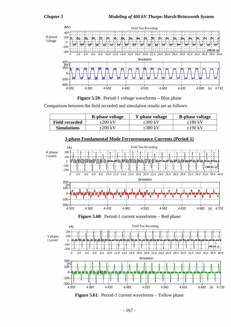
Chapter 5 Modeling of 400 kV Thorpe-Marsh/Brinsworth System
- 167 -
Figure 5.59: Period-1 voltage waveforms – Blue phase
Comparison between the field recorded and simulation results are as follows:
R-phase voltage Y-phase voltage B-phase voltage Field recorded ±200 kV ±300 kV ±180 kV
Simulations ±200 kV ±380 kV ±190 kV
3-phase Fundamental Mode Ferroresonance Currents (Period-1)
Figure 5.60: Period-1 current waveforms – Red phase
Figure 5.61: Period-1 current waveforms – Yellow phase
100 200
0
-200 -100
0 2.0 4.0 6.0 8.0 10.0 12.0 14.0 16.0 18.0 20.0 22.0 24.0 26.0 28.0 30.0 32.0 34.0 36.0 38.0 40.0
(××××0.01 s)
Field Test Recording (A)
4.332 4.382 4.432 4.482 4.532 4.582 4.632 4.682 4.732[s]-200
-100
0
100
200[A]
Simulation
0 2.0 4.0 6.0 8.0 10.0 12.0 14.0 16.0 18.0 20.0 22.0 24.0 26.0 28.0 30.0 32.0 34.0 36.0 38.0 40.0
100 200
0
-200 -100
Field Test Recording (A)
(××××0.01 s)
4.332 4.382 4.432 4.482 4.532 4.582 4.632 4.682 4.732[s]-200
-100
0
100
200[A]
Simulation
0 2.0 4.0 6.0 8.0 10.0 12.0 14.0 16.0 18.0 20.0 22.0 24.0 26.0 28.0 30.0 32.0 34.0 36.0 38.0 40.0 (××××0.01 s)
Field Test Recording (kV)
200 400
-400
0
-200
4.332 4.382 4.432 4.482 4.532 4.582 4.632 4.682 4.732[s]-400
-200
0
200
400[kV]
Simulation
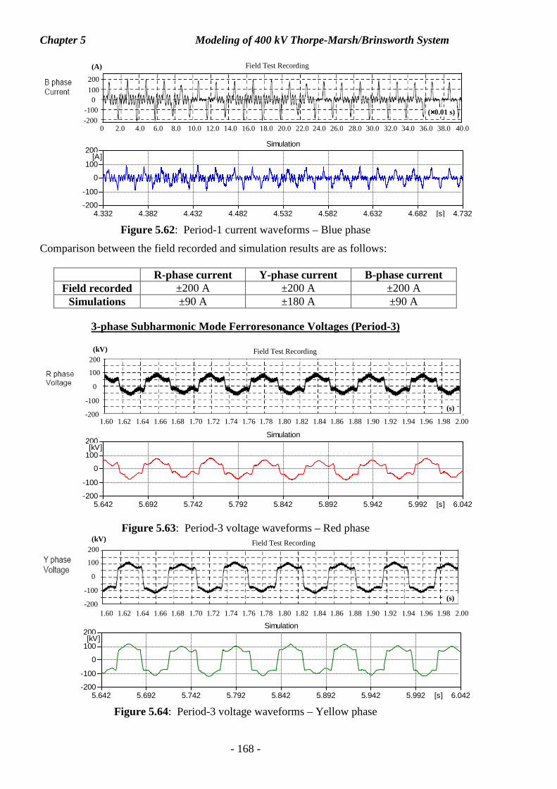
Chapter 5 Modeling of 400 kV Thorpe-Marsh/Brinsworth System
- 168 -
Figure 5.62: Period-1 current waveforms – Blue phase
Comparison between the field recorded and simulation results are as follows:
R-phase current Y-phase current B-phase current Field recorded ±200 A ±200 A ±200 A
Simulations ±90 A ±180 A ±90 A
3-phase Subharmonic Mode Ferroresonance Voltages (Period-3)
Figure 5.63: Period-3 voltage waveforms – Red phase
Figure 5.64: Period-3 voltage waveforms – Yellow phase
(s)
Field Test Recording (kV)
100 200
-200
0
-100
1.60 1.62 1.64 1.66 1.68 1.70 1.72 1.74 1.76 1.78 1.80 1.82 1.84 1.86 1.88 1.90 1.92 1.94 1.96 1.98 2.00
5.642 5.692 5.742 5.792 5.842 5.892 5.942 5.992 6.042[s]-200
-100
0
100
200[kV]
Simulation
(s)
Field Test Recording (kV)
100 200
0
-100
-200 1.60 1.62 1.64 1.66 1.68 1.70 1.72 1.74 1.76 1.78 1.80 1.82 1.84 1.86 1.88 1.90 1.92 1.94 1.96 1.98 2.00
5.642 5.692 5.742 5.792 5.842 5.892 5.942 5.992 6.042[s]-200
-100
0
100
200[kV]
Simulation
100 200
0
-200 -100
Field Test Recording (A)
0 2.0 4.0 6.0 8.0 10.0 12.0 14.0 16.0 18.0 20.0 22.0 24.0 26.0 28.0 30.0 32.0 34.0 36.0 38.0 40.0
(××××0.01 s)
4.332 4.382 4.432 4.482 4.532 4.582 4.632 4.682 4.732[s]-200
-100
0
100
200[A]
Simulation
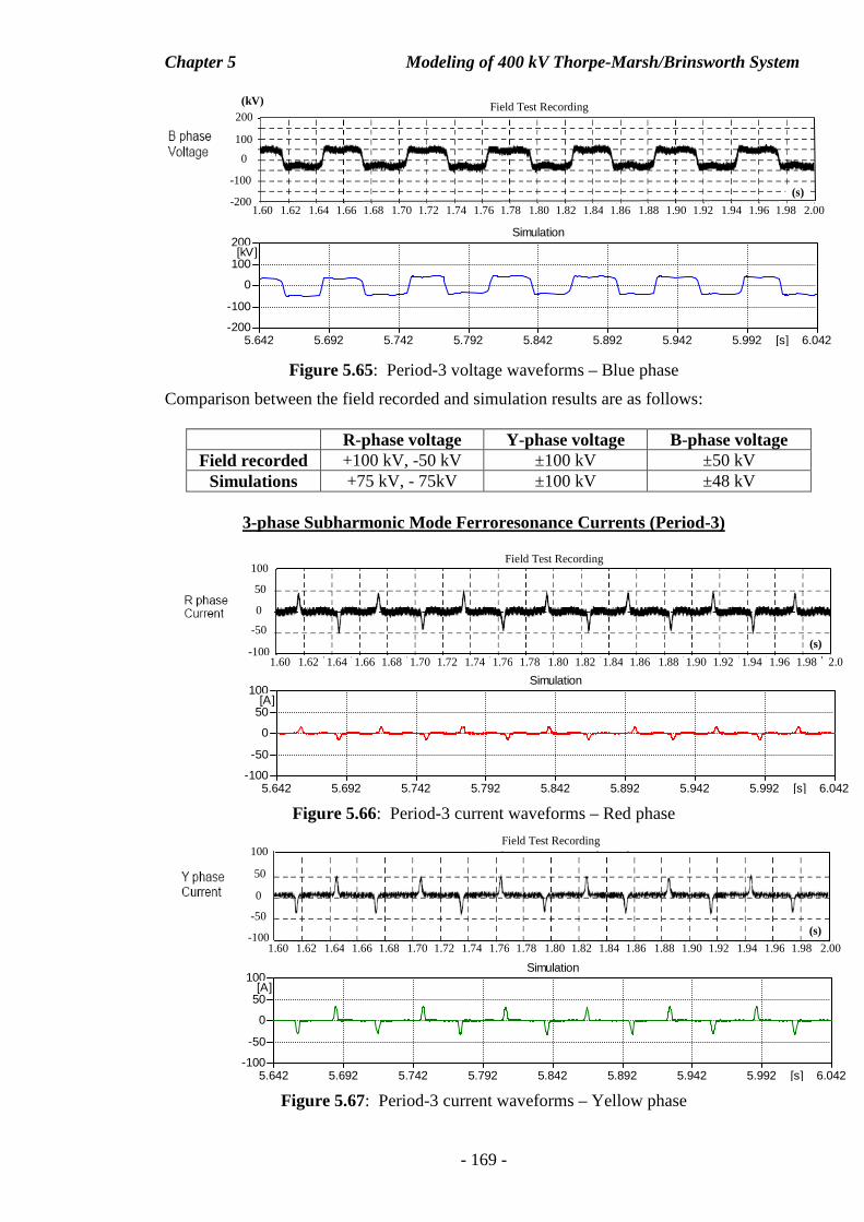
Chapter 5 Modeling of 400 kV Thorpe-Marsh/Brinsworth System
- 169 -
Figure 5.65: Period-3 voltage waveforms – Blue phase
Comparison between the field recorded and simulation results are as follows:
R-phase voltage Y-phase voltage B-phase voltage Field recorded +100 kV, -50 kV ±100 kV ±50 kV
Simulations +75 kV, - 75kV ±100 kV ±48 kV
3-phase Subharmonic Mode Ferroresonance Currents (Period-3)
Figure 5.66: Period-3 current waveforms – Red phase
Figure 5.67: Period-3 current waveforms – Yellow phase
-50
50
100
-100
0
(s)
1.60 1.62 1.64 1.66 1.68 1.70 1.72 1.74 1.76 1.78 1.80 1.82 1.84 1.86 1.88 1.90 1.92 1.94 1.96 1.98 2.00
Field Test Recording
5.642 5.692 5.742 5.792 5.842 5.892 5.942 5.992 6.042[s]-100
-50
0
50
100[A]
Simulation
-50
50
100
-100
0
1.60 1.62 1.64 1.66 1.68 1.70 1.72 1.74 1.76 1.78 1.80 1.82 1.84 1.86 1.88 1.90 1.92 1.94 1.96 1.98 2.0
Field Test Recording
(s)
5.642 5.692 5.742 5.792 5.842 5.892 5.942 5.992 6.042[s]-100
-50
0
50
100[A]
Simulation
(s)
Field Test Recording (kV)
100 200
0
-100
1.60 1.62 1.64 1.66 1.68 1.70 1.72 1.74 1.76 1.78 1.80 1.82 1.84 1.86 1.88 1.90 1.92 1.94 1.96 1.98 2.00 -200
5.642 5.692 5.742 5.792 5.842 5.892 5.942 5.992 6.042[s]-200
-100
0
100
200[kV]
Simulation
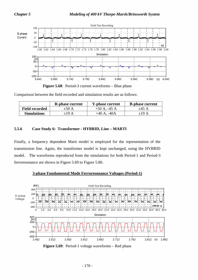
Chapter 5 Modeling of 400 kV Thorpe-Marsh/Brinsworth System
- 170 -
Figure 5.68: Period-3 current waveforms – Blue phase
Comparison between the field recorded and simulation results are as follows:
R-phase current Y-phase current B-phase current Field recorded ±50 A +50 A, -45 A ±45 A
Simulations ±19 A +40 A, -40A ±19 A
5.5.6 Case Study 6: Transformer - HYBRID, Line – MARTI
Finally, a frequency dependent Marti model is employed for the representation of the
transmission line. Again, the transformer model is kept unchanged, using the HYBRID
model. The waveforms reproduced from the simulations for both Period-1 and Period-3
ferroresonance are shown in Figure 5.69 to Figure 5.80.
3-phase Fundamental Mode Ferroresonance Voltages (Period-1)
Figure 5.69: Period-1 voltage waveforms – Red phase
200 400
0
-400
-200
0 2.0 4.0 6.0 8.0 10.0 12.0 14.0 16.0 18.0 20.0 22.0 24.0 26.0 28.0 30.0 32.0 34.0 36.0 38.0 40.0
Field Test Recording (kV)
(××××0.01 s)
2.462 2.512 2.562 2.612 2.662 2.712 2.762 2.812 2.862[s]-400
-200
0
200
400[kV]
Simulation
-50
50
100
-100
0
(s)
1.60 1.62 1.64 1.66 1.68 1.70 1.72 1.74 1.76 1.78 1.80 1.82 1.84 1.86 1.88 1.90 1.92 1.94 1.96 1.98 2.00
Field Test Recording
5.642 5.692 5.742 5.792 5.842 5.892 5.942 5.992 6.042[s]-100
-50
0
50
100[A]
Simulation
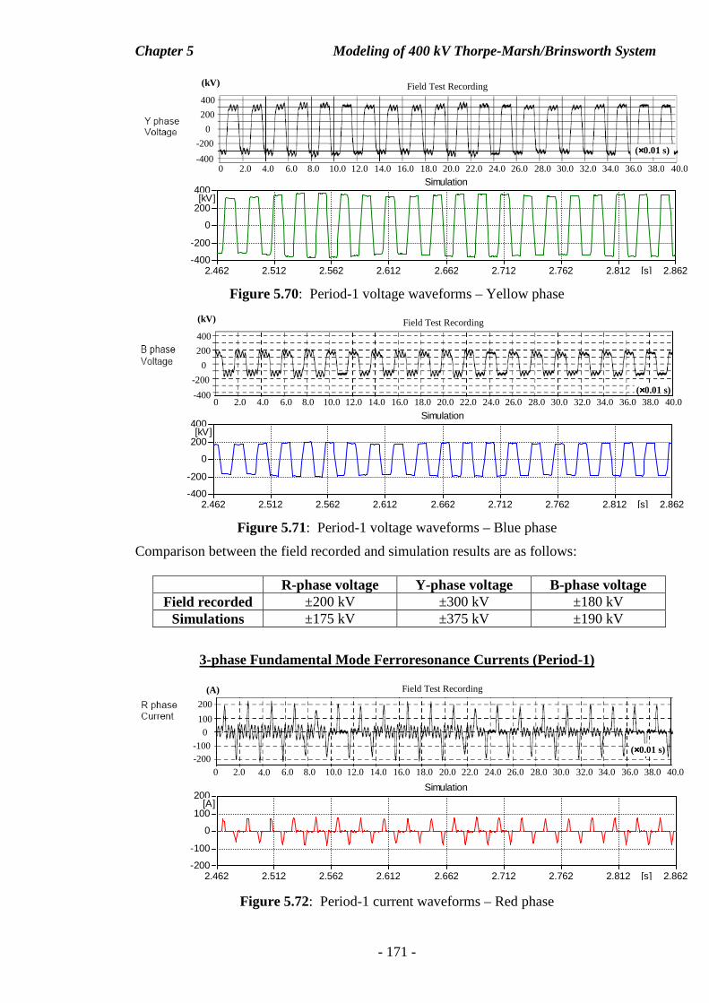
Chapter 5 Modeling of 400 kV Thorpe-Marsh/Brinsworth System
- 171 -
Figure 5.70: Period-1 voltage waveforms – Yellow phase
Figure 5.71: Period-1 voltage waveforms – Blue phase
Comparison between the field recorded and simulation results are as follows:
R-phase voltage Y-phase voltage B-phase voltage Field recorded ±200 kV ±300 kV ±180 kV
Simulations ±175 kV ±375 kV ±190 kV
3-phase Fundamental Mode Ferroresonance Currents (Period-1)
Figure 5.72: Period-1 current waveforms – Red phase
0 2.0 4.0 6.0 8.0 10.0 12.0 14.0 16.0 18.0 20.0 22.0 24.0 26.0 28.0 30.0 32.0 34.0 36.0 38.0 40.0
100 200
0
-200 -100
Field Test Recording (A)
(××××0.01 s)
2.462 2.512 2.562 2.612 2.662 2.712 2.762 2.812 2.862[s]-200
-100
0
100
200[A]
Simulation
0 2.0 4.0 6.0 8.0 10.0 12.0 14.0 16.0 18.0 20.0 22.0 24.0 26.0 28.0 30.0 32.0 34.0 36.0 38.0 40.0
Field Test Recording (kV)
200 400
-400
-200
0
(××××0.01 s)
2.462 2.512 2.562 2.612 2.662 2.712 2.762 2.812 2.862[s]-400
-200
0
200
400[kV]
Simulation
0 2.0 4.0 6.0 8.0 10.0 12.0 14.0 16.0 18.0 20.0 22.0 24.0 26.0 28.0 30.0 32.0 34.0 36.0 38.0 40.0 (××××0.01 s)
Field Test Recording (kV)
200 400
-400
0
-200
2.462 2.512 2.562 2.612 2.662 2.712 2.762 2.812 2.862[s]-400
-200
0
200
400[kV]
Simulation
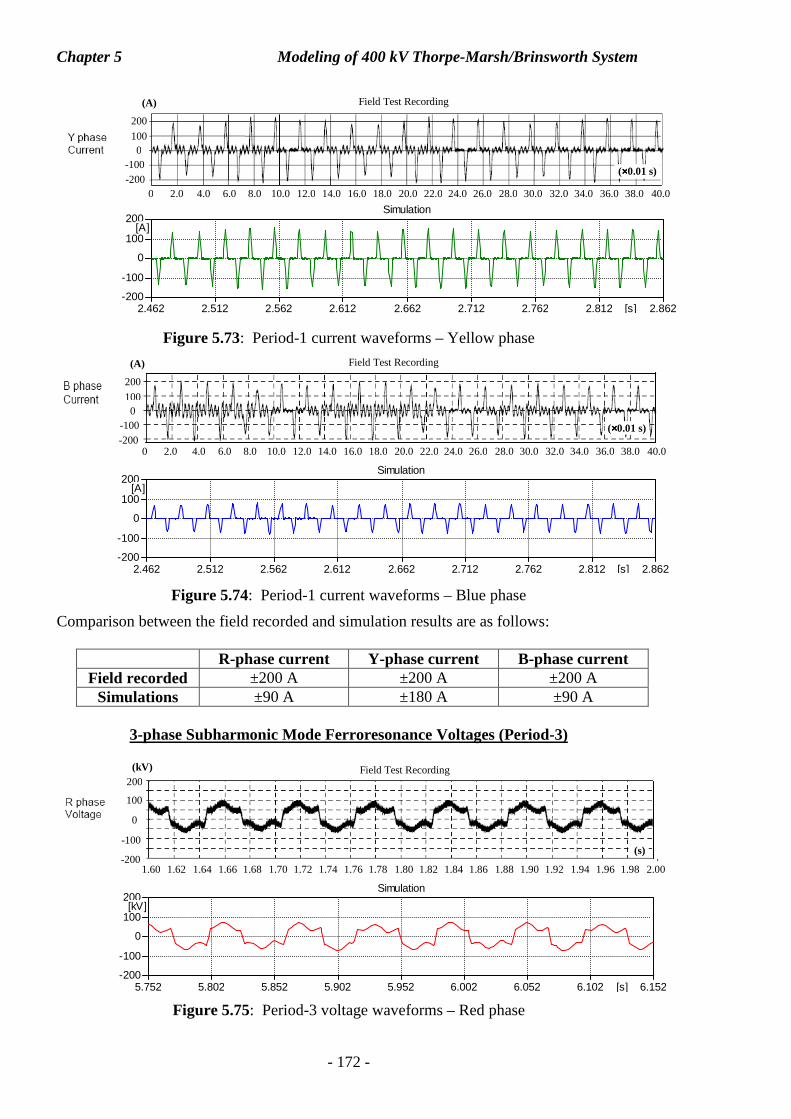
Chapter 5 Modeling of 400 kV Thorpe-Marsh/Brinsworth System
- 172 -
Figure 5.73: Period-1 current waveforms – Yellow phase
Figure 5.74: Period-1 current waveforms – Blue phase
Comparison between the field recorded and simulation results are as follows:
R-phase current Y-phase current B-phase current Field recorded ±200 A ±200 A ±200 A
Simulations ±90 A ±180 A ±90 A
3-phase Subharmonic Mode Ferroresonance Voltages (Period-3)
Figure 5.75: Period-3 voltage waveforms – Red phase
(s)
Field Test Recording (kV)
100 200
0
-100
-200 1.60 1.62 1.64 1.66 1.68 1.70 1.72 1.74 1.76 1.78 1.80 1.82 1.84 1.86 1.88 1.90 1.92 1.94 1.96 1.98 2.00
5.752 5.802 5.852 5.902 5.952 6.002 6.052 6.102 6.152[s]-200
-100
0
100
200[kV]
Simulation
100 200
0
-200 -100
Field Test Recording (A)
0 2.0 4.0 6.0 8.0 10.0 12.0 14.0 16.0 18.0 20.0 22.0 24.0 26.0 28.0 30.0 32.0 34.0 36.0 38.0 40.0
(××××0.01 s)
2.462 2.512 2.562 2.612 2.662 2.712 2.762 2.812 2.862[s]-200
-100
0
100
200[A]
Simulation
100 200
0
-200 -100
0 2.0 4.0 6.0 8.0 10.0 12.0 14.0 16.0 18.0 20.0 22.0 24.0 26.0 28.0 30.0 32.0 34.0 36.0 38.0 40.0
(××××0.01 s)
Field Test Recording (A)
2.462 2.512 2.562 2.612 2.662 2.712 2.762 2.812 2.862[s]-200
-100
0
100
200[A]
Simulation
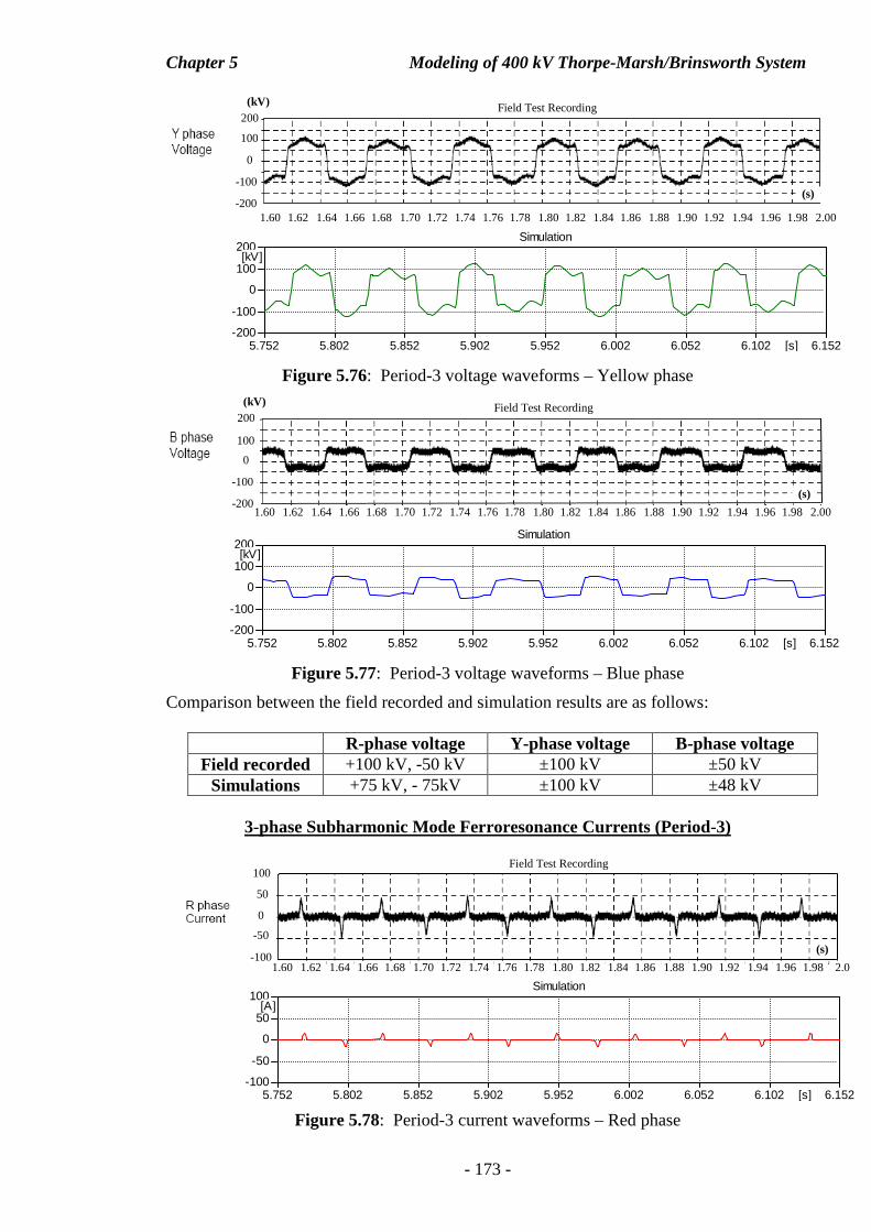
Chapter 5 Modeling of 400 kV Thorpe-Marsh/Brinsworth System
- 173 -
Figure 5.76: Period-3 voltage waveforms – Yellow phase
Figure 5.77: Period-3 voltage waveforms – Blue phase
Comparison between the field recorded and simulation results are as follows:
R-phase voltage Y-phase voltage B-phase voltage Field recorded +100 kV, -50 kV ±100 kV ±50 kV
Simulations +75 kV, - 75kV ±100 kV ±48 kV
3-phase Subharmonic Mode Ferroresonance Currents (Period-3)
Figure 5.78: Period-3 current waveforms – Red phase
-50
50
100
-100
0
1.60 1.62 1.64 1.66 1.68 1.70 1.72 1.74 1.76 1.78 1.80 1.82 1.84 1.86 1.88 1.90 1.92 1.94 1.96 1.98 2.0
Field Test Recording
(s)
5.752 5.802 5.852 5.902 5.952 6.002 6.052 6.102 6.152[s]-100
-50
0
50
100[A]
Simulation
(s)
Field Test Recording (kV)
100 200
0
-100
1.60 1.62 1.64 1.66 1.68 1.70 1.72 1.74 1.76 1.78 1.80 1.82 1.84 1.86 1.88 1.90 1.92 1.94 1.96 1.98 2.00 -200
5.752 5.802 5.852 5.902 5.952 6.002 6.052 6.102 6.152[s]-200
-100
0
100
200[kV]
Simulation
(s)
Field Test Recording (kV)
100 200
-200
0
-100
1.60 1.62 1.64 1.66 1.68 1.70 1.72 1.74 1.76 1.78 1.80 1.82 1.84 1.86 1.88 1.90 1.92 1.94 1.96 1.98 2.00
5.752 5.802 5.852 5.902 5.952 6.002 6.052 6.102 6.152[s]-200
-100
0
100
200[kV]
Simulation
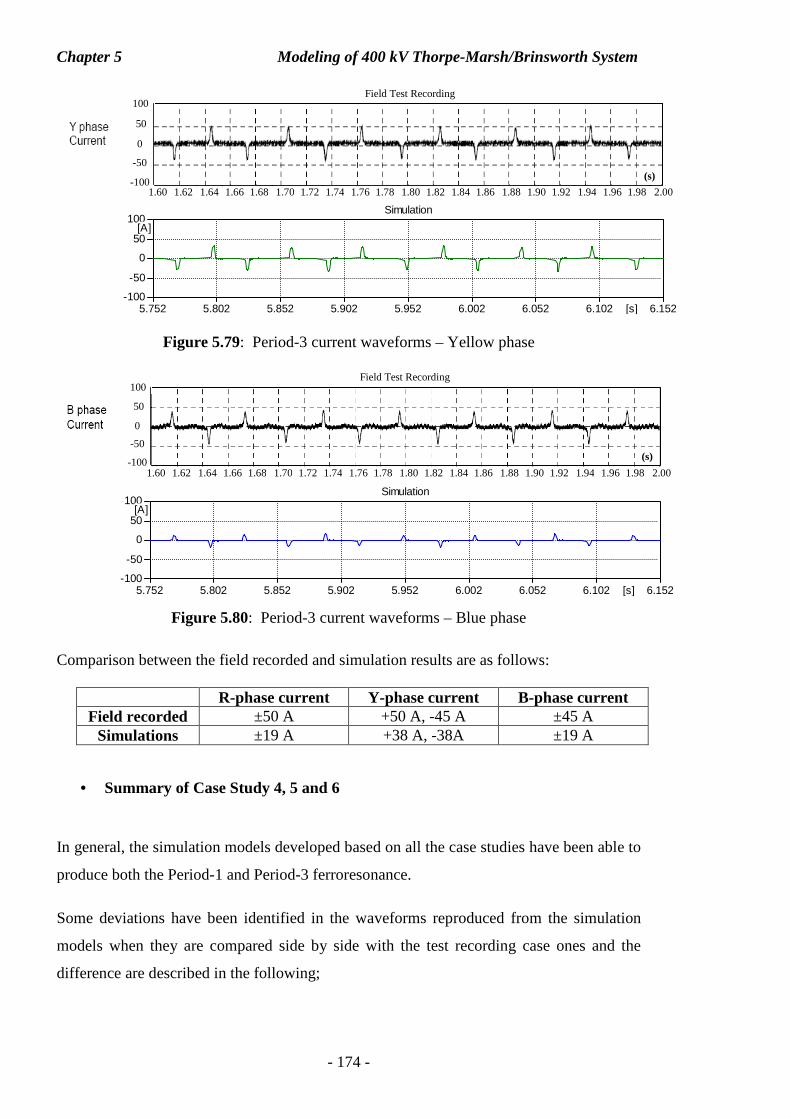
Chapter 5 Modeling of 400 kV Thorpe-Marsh/Brinsworth System
- 174 -
Figure 5.79: Period-3 current waveforms – Yellow phase
Figure 5.80: Period-3 current waveforms – Blue phase
Comparison between the field recorded and simulation results are as follows:
R-phase current Y-phase current B-phase current Field recorded ±50 A +50 A, -45 A ±45 A
Simulations ±19 A +38 A, -38A ±19 A
• Summary of Case Study 4, 5 and 6
In general, the simulation models developed based on all the case studies have been able to
produce both the Period-1 and Period-3 ferroresonance.
Some deviations have been identified in the waveforms reproduced from the simulation
models when they are compared side by side with the test recording case ones and the
difference are described in the following;
5.752 5.802 5.852 5.902 5.952 6.002 6.052 6.102 6.152[s]-100
-50
0
50
100[A]
Simulation
-50
50
100
-100
0
(s)
1.60 1.62 1.64 1.66 1.68 1.70 1.72 1.74 1.76 1.78 1.80 1.82 1.84 1.86 1.88 1.90 1.92 1.94 1.96 1.98 2.00
Field Test Recording
-50
50
100
-100
0
(s)
1.60 1.62 1.64 1.66 1.68 1.70 1.72 1.74 1.76 1.78 1.80 1.82 1.84 1.86 1.88 1.90 1.92 1.94 1.96 1.98 2.00
Field Test Recording
5.752 5.802 5.852 5.902 5.952 6.002 6.052 6.102 6.152[s]-100
-50
0
50
100[A]
Simulation
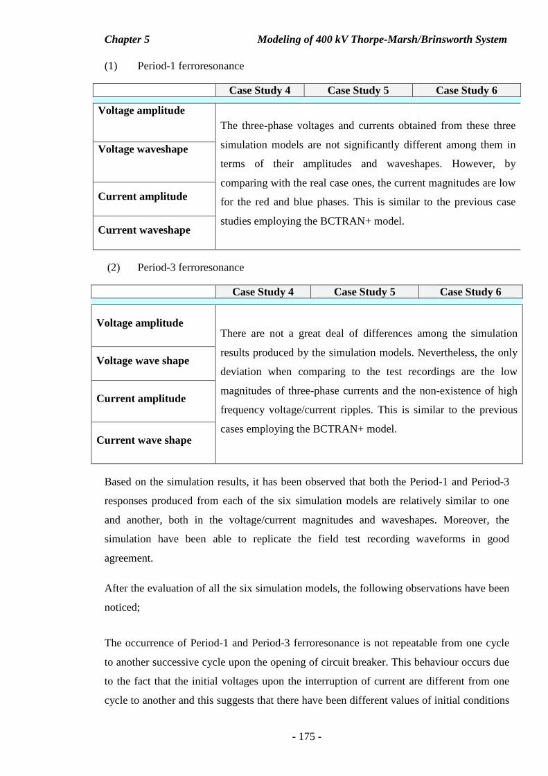
Chapter 5 Modeling of 400 kV Thorpe-Marsh/Brinsworth System
- 175 -
(1) Period-1 ferroresonance
Case Study 4 Case Study 5 Case Study 6
Voltage amplitude
Voltage waveshape
Current amplitude
Current waveshape
The three-phase voltages and currents obtained from these three
simulation models are not significantly different among them in
terms of their amplitudes and waveshapes. However, by
comparing with the real case ones, the current magnitudes are low
for the red and blue phases. This is similar to the previous case
studies employing the BCTRAN+ model.
(2) Period-3 ferroresonance
Case Study 4 Case Study 5 Case Study 6
Voltage amplitude
Voltage wave shape
Current amplitude
Current wave shape
There are not a great deal of differences among the simulation
results produced by the simulation models. Nevertheless, the only
deviation when comparing to the test recordings are the low
magnitudes of three-phase currents and the non-existence of high
frequency voltage/current ripples. This is similar to the previous
cases employing the BCTRAN+ model.
Based on the simulation results, it has been observed that both the Period-1 and Period-3
responses produced from each of the six simulation models are relatively similar to one
and another, both in the voltage/current magnitudes and waveshapes. Moreover, the
simulation have been able to replicate the field test recording waveforms in good
agreement.
After the evaluation of all the six simulation models, the following observations have been
noticed;
The occurrence of Period-1 and Period-3 ferroresonance is not repeatable from one cycle
to another successive cycle upon the opening of circuit breaker. This behaviour occurs due
to the fact that the initial voltages upon the interruption of current are different from one
cycle to another and this suggests that there have been different values of initial conditions
Chapter 5 Modeling of 400 kV Thorpe-Marsh/Brinsworth System
- 176 -
being applied to the system. The system is triggered with different voltage points which
can be sensitive for the initiation of different responses. This kind of behaviour has also
been experienced by [13, 14] in which different steady state responses can be induced
simply due to small changes in system parameters or initial conditions. In view of this
behaviour, there have been a great deal of simulations being carried out in order for the
system to be able to exhibit the type of required ferroresonant response. That is the reason
that a large amount of simulations lasting for a few cycles are sometimes required for the
determination of both the Period-1 and Period-3 responses. Furthermore, from the UK
perspective as quoted in [72], the onset of this type of phenomena has been considered as
random or stochastic which is dependent on system parameters. In addition, [11]
mentioned that the nonlinear system of ferroresonance condition is extremely susceptible
to changes in system parameters and initial conditions. The system can induce different
responses upon a small change of system voltage, capacitance or losses. [17] described that
ferroresonance phenomena relied on (1) the degree of transformer’s residual flux, (2) the
initial charge of the capacitive elements and (3) the point on the voltage wave.
The major limitations that all the six simulation models have are explained as follows;
(1) Period-1 ferroresonance
Case Study 1, 2, 3, 4, 5 and 6 Limitation The magnitudes of the red and blue phase currents that have been reproduced
from all the simulation models are only 50% of the measurement ones.
(2) Period-3 ferroresonance
Case Study 1, 2, 3, 4, 5 and 6 Limitation The magnitudes of the three-phase currents reproduced from the simulation
models are relatively small as compared to the real case ones. Furthermore,
both the voltages and currents that have been reproduced do not contain any
high frequency ripples as expected from the real ones.
Due to the limitations of the simulation models therefore the next step is to improve one of
the six models by looking into a possible way to modify the parameter of either the
transformer or the transmission line models. The following questions arise before
modification takes place.
(1) Which simulation model out of six is the best choice to be employed for
improvement?
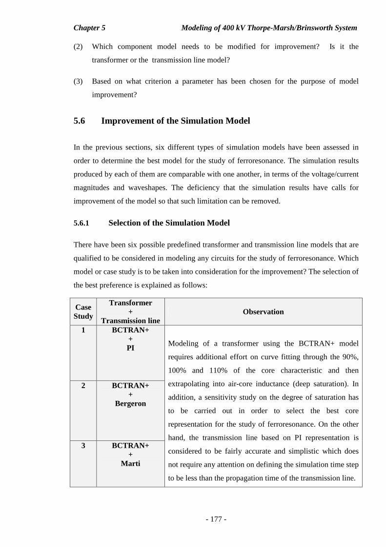
Chapter 5 Modeling of 400 kV Thorpe-Marsh/Brinsworth System
- 177 -
(2) Which component model needs to be modified for improvement? Is it the
transformer or the transmission line model?
(3) Based on what criterion a parameter has been chosen for the purpose of model
improvement?
5.6 Improvement of the Simulation Model
In the previous sections, six different types of simulation models have been assessed in
order to determine the best model for the study of ferroresonance. The simulation results
produced by each of them are comparable with one another, in terms of the voltage/current
magnitudes and waveshapes. The deficiency that the simulation results have calls for
improvement of the model so that such limitation can be removed.
5.6.1 Selection of the Simulation Model
There have been six possible predefined transformer and transmission line models that are
qualified to be considered in modeling any circuits for the study of ferroresonance. Which
model or case study is to be taken into consideration for the improvement? The selection of
the best preference is explained as follows:
Case Study
Transformer +
Transmission line Observation
1 BCTRAN+ + PI
2 BCTRAN+ +
Bergeron
3 BCTRAN+ +
Marti
Modeling of a transformer using the BCTRAN+ model
requires additional effort on curve fitting through the 90%,
100% and 110% of the core characteristic and then
extrapolating into air-core inductance (deep saturation). In
addition, a sensitivity study on the degree of saturation has
to be carried out in order to select the best core
representation for the study of ferroresonance. On the other
hand, the transmission line based on PI representation is
considered to be fairly accurate and simplistic which does
not require any attention on defining the simulation time step
to be less than the propagation time of the transmission line.
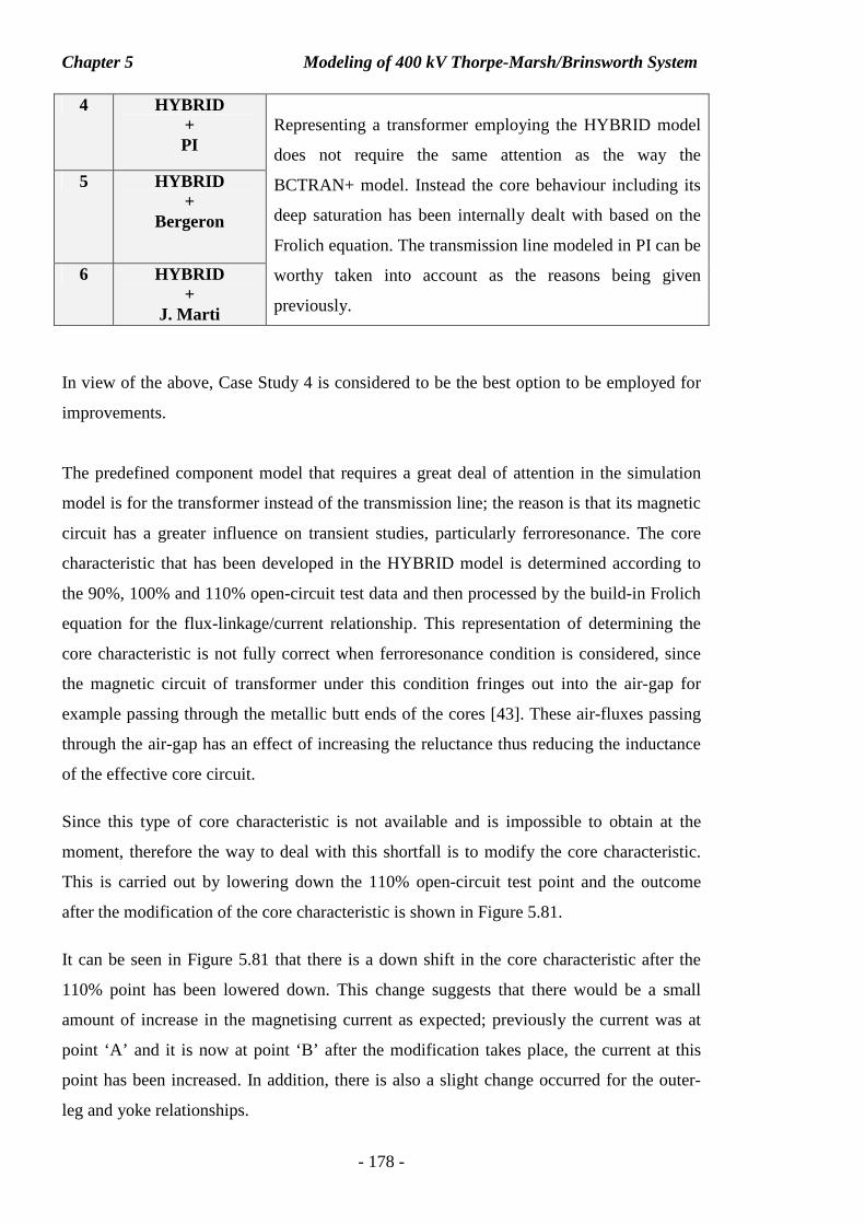
Chapter 5 Modeling of 400 kV Thorpe-Marsh/Brinsworth System
- 178 -
4 HYBRID + PI
5 HYBRID +
Bergeron
6 HYBRID +
J. Marti
Representing a transformer employing the HYBRID model
does not require the same attention as the way the
BCTRAN+ model. Instead the core behaviour including its
deep saturation has been internally dealt with based on the
Frolich equation. The transmission line modeled in PI can be
worthy taken into account as the reasons being given
previously.
In view of the above, Case Study 4 is considered to be the best option to be employed for
improvements.
The predefined component model that requires a great deal of attention in the simulation
model is for the transformer instead of the transmission line; the reason is that its magnetic
circuit has a greater influence on transient studies, particularly ferroresonance. The core
characteristic that has been developed in the HYBRID model is determined according to
the 90%, 100% and 110% open-circuit test data and then processed by the build-in Frolich
equation for the flux-linkage/current relationship. This representation of determining the
core characteristic is not fully correct when ferroresonance condition is considered, since
the magnetic circuit of transformer under this condition fringes out into the air-gap for
example passing through the metallic butt ends of the cores [43]. These air-fluxes passing
through the air-gap has an effect of increasing the reluctance thus reducing the inductance
of the effective core circuit.
Since this type of core characteristic is not available and is impossible to obtain at the
moment, therefore the way to deal with this shortfall is to modify the core characteristic.
This is carried out by lowering down the 110% open-circuit test point and the outcome
after the modification of the core characteristic is shown in Figure 5.81.
It can be seen in Figure 5.81 that there is a down shift in the core characteristic after the
110% point has been lowered down. This change suggests that there would be a small
amount of increase in the magnetising current as expected; previously the current was at
point ‘A’ and it is now at point ‘B’ after the modification takes place, the current at this
point has been increased. In addition, there is also a slight change occurred for the outer-
leg and yoke relationships.
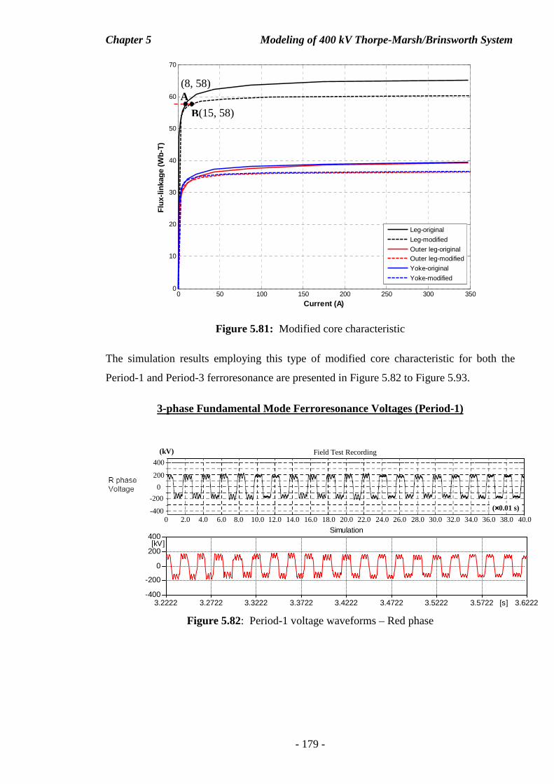
Chapter 5 Modeling of 400 kV Thorpe-Marsh/Brinsworth System
- 179 -
Figure 5.81: Modified core characteristic
The simulation results employing this type of modified core characteristic for both the
Period-1 and Period-3 ferroresonance are presented in Figure 5.82 to Figure 5.93.
3-phase Fundamental Mode Ferroresonance Voltages (Period-1)
Figure 5.82: Period-1 voltage waveforms – Red phase
200 400
0
-400
-200
0 2.0 4.0 6.0 8.0 10.0 12.0 14.0 16.0 18.0 20.0 22.0 24.0 26.0 28.0 30.0 32.0 34.0 36.0 38.0 40.0
Field Test Recording (kV)
(××××0.01 s)
0 50 100 150 200 250 300 3500
10
20
30
40
50
60
70
Current (A)
Flux
-link
age
(Wb-
T)
Leg-original
Leg-modified
Outer leg-originalOuter leg-modified
Yoke-original
Yoke-modified
A
B
(8, 58)
(15, 58)
3.2222 3.2722 3.3222 3.3722 3.4222 3.4722 3.5222 3.5722 3.6222[s]-400
-200
0
200
400[kV]
Simulation
Chapter 5 Modeling of 400 kV Thorpe-Marsh/Brinsworth System
- 180 -
Figure 5.83: Period-1 voltage waveforms – Yellow phase
Figure 5.84: Period-1 voltage waveforms – Blue phase
Comparison between the field recorded and simulation results are as follows:
R-phase voltage Y-phase voltage B-phase voltage Field recorded ±200 kV ±300 kV ±180 kV
Simulations ±175 kV ±300 kV ±180 kV
Simulations results show that there is slight improvement on the magnitude of the Y-phase
voltage.
0 2.0 4.0 6.0 8.0 10.0 12.0 14.0 16.0 18.0 20.0 22.0 24.0 26.0 28.0 30.0 32.0 34.0 36.0 38.0 40.0
Field Test Recording (kV)
200 400
-400
-200
0
(××××0.01 s)
0 2.0 4.0 6.0 8.0 10.0 12.0 14.0 16.0 18.0 20.0 22.0 24.0 26.0 28.0 30.0 32.0 34.0 36.0 38.0 40.0 (××××0.01 s)
Field Test Recording (kV)
200 400
-400
0
-200
3.2222 3.2722 3.3222 3.3722 3.4222 3.4722 3.5222 3.5722 3.6222[s]-400
-200
0
200
400[kV]
Simulation
3.2222 3.2722 3.3222 3.3722 3.4222 3.4722 3.5222 3.5722 3.6222[s]-400
-200
0
200
400[kV]
Simulation
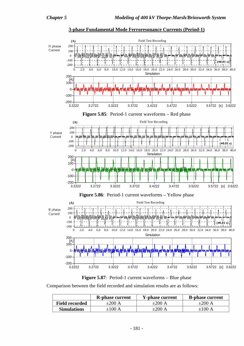
Chapter 5 Modeling of 400 kV Thorpe-Marsh/Brinsworth System
- 181 -
3-phase Fundamental Mode Ferroresonance Currents (Period-1)
Figure 5.85: Period-1 current waveforms – Red phase
Figure 5.86: Period-1 current waveforms – Yellow phase
Figure 5.87: Period-1 current waveforms – Blue phase
Comparison between the field recorded and simulation results are as follows:
R-phase current Y-phase current B-phase current Field recorded ±200 A ±200 A ±200 A
Simulations ±100 A ±200 A ±100 A
100 200
0
-200 -100
Field Test Recording (A)
0 2.0 4.0 6.0 8.0 10.0 12.0 14.0 16.0 18.0 20.0 22.0 24.0 26.0 28.0 30.0 32.0 34.0 36.0 38.0 40.0
(××××0.01 s)
3.2222 3.2722 3.3222 3.3722 3.4222 3.4722 3.5222 3.5722 3.6222[s]-200
-100
0
100
200[A]
Simulation
100 200
0
-200 -100
0 2.0 4.0 6.0 8.0 10.0 12.0 14.0 16.0 18.0 20.0 22.0 24.0 26.0 28.0 30.0 32.0 34.0 36.0 38.0 40.0
(××××0.01 s)
Field Test Recording (A)
3.2222 3.2722 3.3222 3.3722 3.4222 3.4722 3.5222 3.5722 3.6222[s]-200
-100
0
100
200[A]
Simulation
0 2.0 4.0 6.0 8.0 10.0 12.0 14.0 16.0 18.0 20.0 22.0 24.0 26.0 28.0 30.0 32.0 34.0 36.0 38.0 40.0
100 200
0
-200 -100
Field Test Recording (A)
(××××0.01 s)
3.2222 3.2722 3.3222 3.3722 3.4222 3.4722 3.5222 3.5722 3.6222[s]-200
-100
0
100
200[A]
Simulation
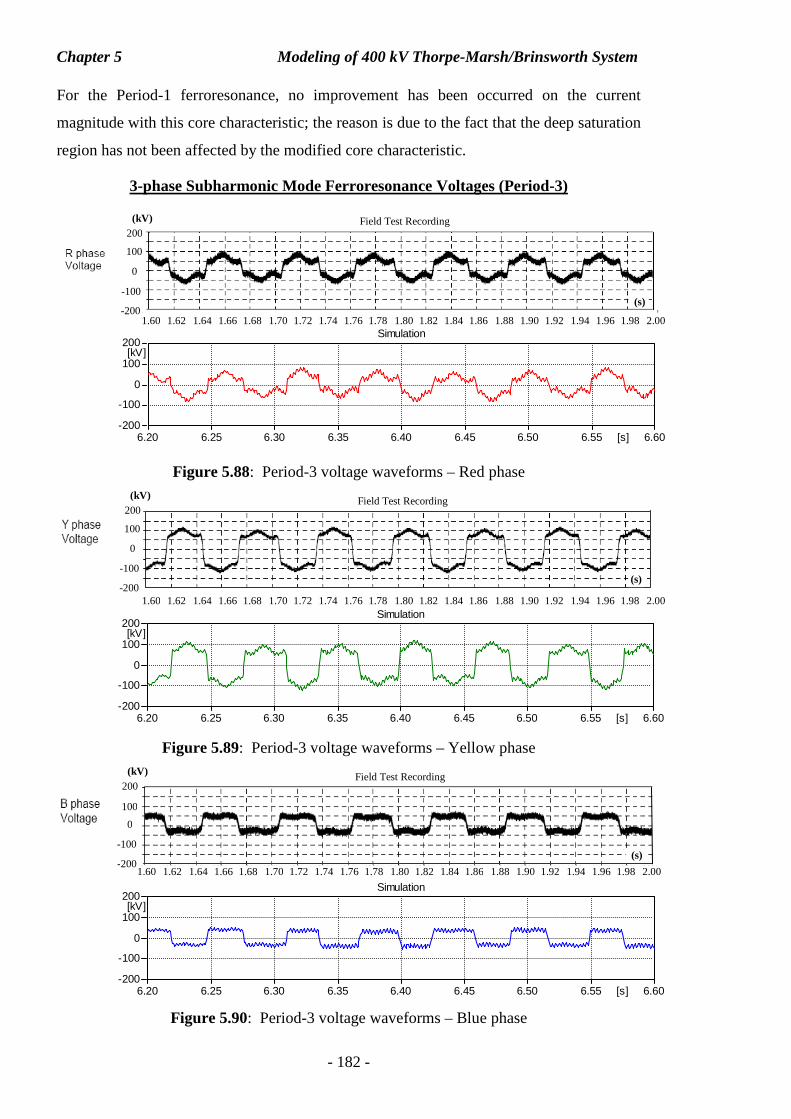
Chapter 5 Modeling of 400 kV Thorpe-Marsh/Brinsworth System
- 182 -
For the Period-1 ferroresonance, no improvement has been occurred on the current
magnitude with this core characteristic; the reason is due to the fact that the deep saturation
region has not been affected by the modified core characteristic.
3-phase Subharmonic Mode Ferroresonance Voltages (Period-3)
Figure 5.88: Period-3 voltage waveforms – Red phase
Figure 5.89: Period-3 voltage waveforms – Yellow phase
Figure 5.90: Period-3 voltage waveforms – Blue phase
(s)
Field Test Recording (kV)
100 200
0
-100
1.60 1.62 1.64 1.66 1.68 1.70 1.72 1.74 1.76 1.78 1.80 1.82 1.84 1.86 1.88 1.90 1.92 1.94 1.96 1.98 2.00 -200
(s)
Field Test Recording (kV)
100 200
-200
0
-100
1.60 1.62 1.64 1.66 1.68 1.70 1.72 1.74 1.76 1.78 1.80 1.82 1.84 1.86 1.88 1.90 1.92 1.94 1.96 1.98 2.00
6.20 6.25 6.30 6.35 6.40 6.45 6.50 6.55 6.60[s]-200
-100
0
100
200[kV]
Simulation
(s)
Field Test Recording (kV)
100 200
0
-100
-200 1.60 1.62 1.64 1.66 1.68 1.70 1.72 1.74 1.76 1.78 1.80 1.82 1.84 1.86 1.88 1.90 1.92 1.94 1.96 1.98 2.00
6.20 6.25 6.30 6.35 6.40 6.45 6.50 6.55 6.60[s]-200
-100
0
100
200[kV]
Simulation
6.20 6.25 6.30 6.35 6.40 6.45 6.50 6.55 6.60[s]-200
-100
0
100
200[kV]
Simulation
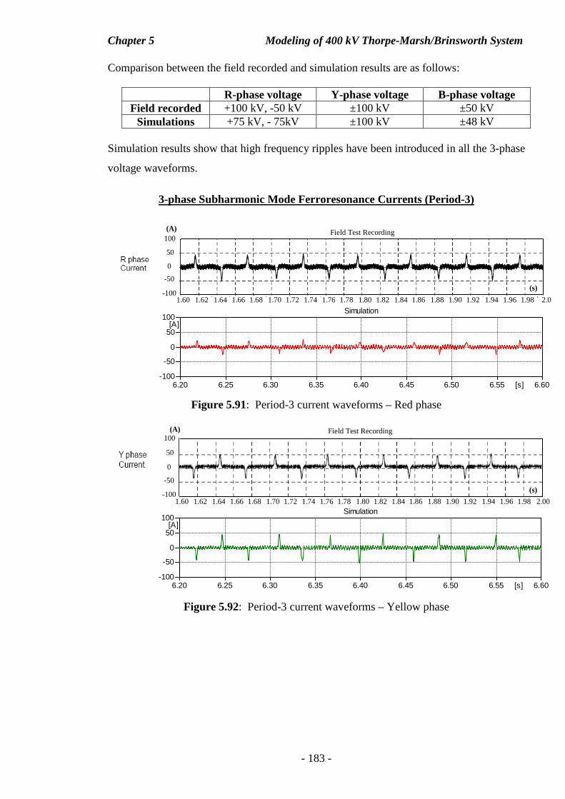
Chapter 5 Modeling of 400 kV Thorpe-Marsh/Brinsworth System
- 183 -
Comparison between the field recorded and simulation results are as follows:
R-phase voltage Y-phase voltage B-phase voltage Field recorded +100 kV, -50 kV ±100 kV ±50 kV
Simulations +75 kV, - 75kV ±100 kV ±48 kV Simulation results show that high frequency ripples have been introduced in all the 3-phase
voltage waveforms.
3-phase Subharmonic Mode Ferroresonance Currents (Period-3)
Figure 5.91: Period-3 current waveforms – Red phase
Figure 5.92: Period-3 current waveforms – Yellow phase
-50
50
100
-100
0
(s)
1.60 1.62 1.64 1.66 1.68 1.70 1.72 1.74 1.76 1.78 1.80 1.82 1.84 1.86 1.88 1.90 1.92 1.94 1.96 1.98 2.00
Field Test Recording (A)
-50
50
100
-100
0
1.60 1.62 1.64 1.66 1.68 1.70 1.72 1.74 1.76 1.78 1.80 1.82 1.84 1.86 1.88 1.90 1.92 1.94 1.96 1.98 2.0
Field Test Recording
(s)
(A)
6.20 6.25 6.30 6.35 6.40 6.45 6.50 6.55 6.60[s]-100
-50
0
50
100[A]
Simulation
6.20 6.25 6.30 6.35 6.40 6.45 6.50 6.55 6.60[s]-100
-50
0
50
100[A]
Simulation
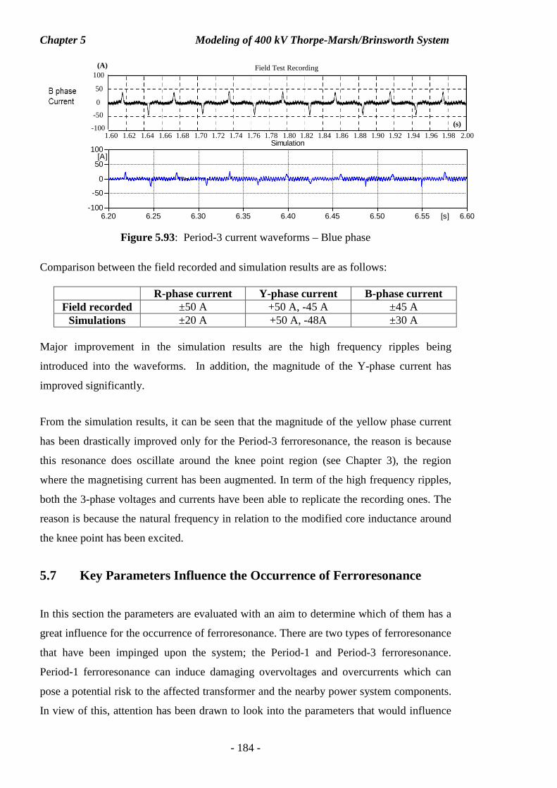
Chapter 5 Modeling of 400 kV Thorpe-Marsh/Brinsworth System
- 184 -
Figure 5.93: Period-3 current waveforms – Blue phase
Comparison between the field recorded and simulation results are as follows:
R-phase current Y-phase current B-phase current Field recorded ±50 A +50 A, -45 A ±45 A
Simulations ±20 A +50 A, -48A ±30 A Major improvement in the simulation results are the high frequency ripples being
introduced into the waveforms. In addition, the magnitude of the Y-phase current has
improved significantly.
From the simulation results, it can be seen that the magnitude of the yellow phase current
has been drastically improved only for the Period-3 ferroresonance, the reason is because
this resonance does oscillate around the knee point region (see Chapter 3), the region
where the magnetising current has been augmented. In term of the high frequency ripples,
both the 3-phase voltages and currents have been able to replicate the recording ones. The
reason is because the natural frequency in relation to the modified core inductance around
the knee point has been excited.
5.7 Key Parameters Influence the Occurrence of Ferroresonance
In this section the parameters are evaluated with an aim to determine which of them has a
great influence for the occurrence of ferroresonance. There are two types of ferroresonance
that have been impinged upon the system; the Period-1 and Period-3 ferroresonance.
Period-1 ferroresonance can induce damaging overvoltages and overcurrents which can
pose a potential risk to the affected transformer and the nearby power system components.
In view of this, attention has been drawn to look into the parameters that would influence
-50
50
100
-100
0
(s)
1.60 1.62 1.64 1.66 1.68 1.70 1.72 1.74 1.76 1.78 1.80 1.82 1.84 1.86 1.88 1.90 1.92 1.94 1.96 1.98 2.00
Field Test Recording
6.20 6.25 6.30 6.35 6.40 6.45 6.50 6.55 6.60[s]-100
-50
0
50
100[A]
Simulation
(A)
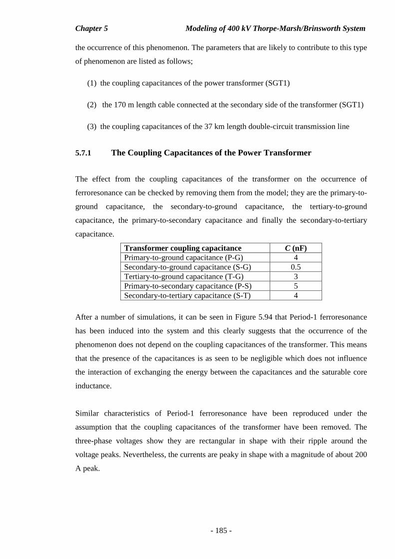
Chapter 5 Modeling of 400 kV Thorpe-Marsh/Brinsworth System
- 185 -
the occurrence of this phenomenon. The parameters that are likely to contribute to this type
of phenomenon are listed as follows;
(1) the coupling capacitances of the power transformer (SGT1)
(2) the 170 m length cable connected at the secondary side of the transformer (SGT1)
(3) the coupling capacitances of the 37 km length double-circuit transmission line
5.7.1 The Coupling Capacitances of the Power Transformer
The effect from the coupling capacitances of the transformer on the occurrence of
ferroresonance can be checked by removing them from the model; they are the primary-to-
ground capacitance, the secondary-to-ground capacitance, the tertiary-to-ground
capacitance, the primary-to-secondary capacitance and finally the secondary-to-tertiary
capacitance.
Transformer coupling capacitance C (nF) Primary-to-ground capacitance (P-G) 4 Secondary-to-ground capacitance (S-G) 0.5 Tertiary-to-ground capacitance (T-G) 3 Primary-to-secondary capacitance (P-S) 5 Secondary-to-tertiary capacitance (S-T) 4
After a number of simulations, it can be seen in Figure 5.94 that Period-1 ferroresonance
has been induced into the system and this clearly suggests that the occurrence of the
phenomenon does not depend on the coupling capacitances of the transformer. This means
that the presence of the capacitances is as seen to be negligible which does not influence
the interaction of exchanging the energy between the capacitances and the saturable core
inductance.
Similar characteristics of Period-1 ferroresonance have been reproduced under the
assumption that the coupling capacitances of the transformer have been removed. The
three-phase voltages show they are rectangular in shape with their ripple around the
voltage peaks. Nevertheless, the currents are peaky in shape with a magnitude of about 200
A peak.
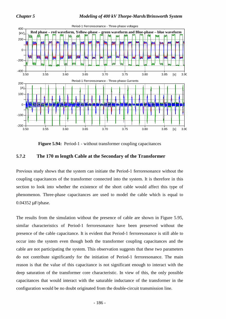
Chapter 5 Modeling of 400 kV Thorpe-Marsh/Brinsworth System
- 186 -
Figure 5.94: Period-1 - without transformer coupling capacitances
5.7.2 The 170 m length Cable at the Secondary of the Transformer
Previous study shows that the system can initiate the Period-1 ferroresonance without the
coupling capacitances of the transformer connected into the system. It is therefore in this
section to look into whether the existence of the short cable would affect this type of
phenomenon. Three-phase capacitances are used to model the cable which is equal to
0.04352 µF/phase.
The results from the simulation without the presence of cable are shown in Figure 5.95,
similar characteristics of Period-1 ferroresonance have been preserved without the
presence of the cable capacitance. It is evident that Period-1 ferroresonance is still able to
occur into the system even though both the transformer coupling capacitances and the
cable are not participating the system. This observation suggests that these two parameters
do not contribute significantly for the initiation of Period-1 ferroresonance. The main
reason is that the value of this capacitance is not significant enough to interact with the
deep saturation of the transformer core characteristic. In view of this, the only possible
capacitances that would interact with the saturable inductance of the transformer in the
configuration would be no doubt originated from the double-circuit transmission line.
3.50 3.55 3.60 3.65 3.70 3.75 3.80 3.85 3.90[s]-400
-200
0
200
400
[kV]
Period-1 Ferroresonance - Three-phase voltages
3.50 3.55 3.60 3.65 3.70 3.75 3.80 3.85 3.90[s]-200
-100
0
100
200
[A]
Period-1 Ferroresonance - Three-phase Currents
Red phase – red waveform, Yellow-phase – green waveform and Blue-phase – blue waveform
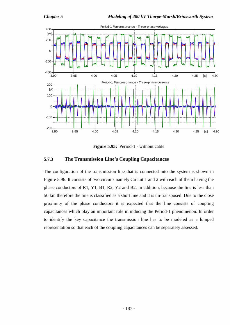
Chapter 5 Modeling of 400 kV Thorpe-Marsh/Brinsworth System
- 187 -
Figure 5.95: Period-1 - without cable
5.7.3 The Transmission Line’s Coupling Capacitances
The configuration of the transmission line that is connected into the system is shown in
Figure 5.96. It consists of two circuits namely Circuit 1 and 2 with each of them having the
phase conductors of R1, Y1, B1, R2, Y2 and B2. In addition, because the line is less than
50 km therefore the line is classified as a short line and it is un-transposed. Due to the close
proximity of the phase conductors it is expected that the line consists of coupling
capacitances which play an important role in inducing the Period-1 phenomenon. In order
to identify the key capacitance the transmission line has to be modeled as a lumped
representation so that each of the coupling capacitances can be separately assessed.
3.90 3.95 4.00 4.05 4.10 4.15 4.20 4.25 4.30[s]-400
-200
0
200
400
[kV]
Period-1 Ferroresonance - Three-phase voltages
3.90 3.95 4.00 4.05 4.10 4.15 4.20 4.25 4.30[s]-200
-100
0
100
200
[A]
Period-1 Ferroresonance - Three-phase currents
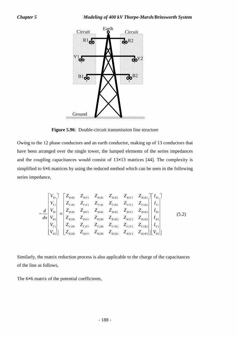
Chapter 5 Modeling of 400 kV Thorpe-Marsh/Brinsworth System
- 188 -
Figure 5.96: Double-circuit transmission line structure
Owing to the 12 phase conductors and an earth conductor, making up of 13 conductors that
have been arranged over the single tower, the lumped elements of the series impedances
and the coupling capacitances would consist of 13×13 matrices [44]. The complexity is
simplified to 6×6 matrices by using the reduced method which can be seen in the following
series impedance,
1 1 1 1 1 1 1 1 2 1 2 1 2
1 1 1 1 1 1 1 1 2 1 2 1 2
1 1 1 1 1 1 1 1 2 1 2 1 2
2 2 1 2 1 2 1 2 2 2 2 2 2
2 2 1 2 1 2 1 2 2 2 2 2 2
2 2 1
R R R R Y R B R R R Y R B
Y Y R Y Y Y B Y R Y Y Y B
B B R B Y B B B R B Y B B
R R R R Y R B R R R Y R B
Y Y R Y Y Y B Y R Y Y Y B
B B R B
V Z Z Z Z Z Z
V Z Z Z Z Z Z
V Z Z Z Z Z Zd
V Z Z Z Z Z Zdx
V Z Z Z Z Z Z
V Z Z
− =
1
1
1
2
2
2 1 2 1 2 2 2 2 2 2 2
R
Y
B
R
Y
Y B B B R B Y B B B
I
I
I
I
I
Z Z Z Z V
(5.2)
Similarly, the matrix reduction process is also applicable to the charge of the capacitances
of the line as follows,
The 6×6 matrix of the potential coefficients,
Earth
R1
Y1
B1
R2
Y2
B2
Ground
Circuit Circuit
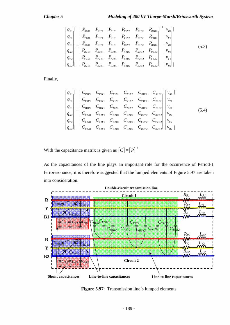
Chapter 5 Modeling of 400 kV Thorpe-Marsh/Brinsworth System
- 189 -
1 1 1 1 1 1 1 1 2 1 2 1 2
1 1 1 1 1 1 1 1 2 1 2 1 2
1 1 1 1 1 1 1 1 2 1 2 1 2
2 2 1 2 1 2 1 2 2 2 2 2 2
2 2 1 2 1 2 1 2 2 2 2 2 2
2 2 1 2 1
R R R R Y R B R R R Y R B
Y Y R Y Y Y B Y R Y Y Y B
B B R B Y B B B R B Y B B
R R R R Y R B R R R Y R B
Y Y R Y Y Y B Y R Y Y Y B
B B R B Y
q P P P P P P
q P P P P P P
q P P P P P P
q P P P P P P
q P P P P P P
q P P P
=
1
1
1
1
2
2
2 1 2 2 2 2 2 2 2
R
Y
B
R
Y
B B B R B Y B B B
v
v
v
v
v
P P P v
−
(5.3)
Finally,
1 1 1 1 1 1 1 1 2 1 2 1 2
1 1 1 1 1 1 1 1 2 1 2 1 2
1 1 1 1 1 1 1 1 2 1 2 1 2
2 2 1 2 1 2 1 2 2 2 2 2 2
2 2 1 2 1 2 1 2 2 2 2 2 2
2 2 1 2 1
R R R R Y R B R R R Y R B
Y Y R Y Y Y B Y R Y Y Y B
B B R B Y B B B R B Y B B
R R R R Y R B R R R Y R B
Y Y R Y Y Y B Y R Y Y Y B
B B R B Y
q C C C C C C
q C C C C C C
q C C C C C C
q C C C C C C
q C C C C C C
q C C C
=
1
1
1
2
2
2 1 2 2 2 2 2 2 2
R
Y
B
R
Y
B B B R B Y B B B
v
v
v
v
v
C C C v
(5.4)
With the capacitance matrix is given as [ ] [ ] 1C P
−=
As the capacitances of the line plays an important role for the occurrence of Period-1
ferroresonance, it is therefore suggested that the lumped elements of Figure 5.97 are taken
into consideration.
Figure 5.97: Transmission line’s lumped elements
Circuit 1
Circuit 2
Double-circuit transmission line
R
Y
B1
R
Y
B2
CR1 CY1 CB1
CR2 CY2 CB2
CR1B1 CR1Y1
CY1B1
CR2Y2
CY2B2
CR2B2
CR1R2 CY1R2
CB1R2 CR1Y2
CY1Y2
CB1Y2 CR1B2
CY1B2
CB1B2
RR1 LR1
RY1 LY1
RB1 LB1
RR2 LB2
RY2 LY2
RB2 LB2
Line-to-line capacitances Shunt capacitances Line-to-line capacitances
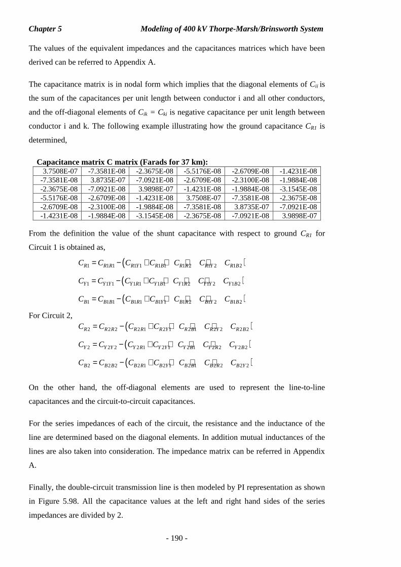
Chapter 5 Modeling of 400 kV Thorpe-Marsh/Brinsworth System
- 190 -
The values of the equivalent impedances and the capacitances matrices which have been
derived can be referred to Appendix A.
The capacitance matrix is in nodal form which implies that the diagonal elements of Cii is
the sum of the capacitances per unit length between conductor i and all other conductors,
and the off-diagonal elements of Cik = Cki is negative capacitance per unit length between
conductor i and k. The following example illustrating how the ground capacitance CR1 is
determined,
Capacitance matrix C matrix (Farads for 37 km): 3.7508E-07 -7.3581E-08 -2.3675E-08 -5.5176E-08 -2.6709E-08 -1.4231E-08
-7.3581E-08 3.8735E-07 -7.0921E-08 -2.6709E-08 -2.3100E-08 -1.9884E-08 -2.3675E-08 -7.0921E-08 3.9898E-07 -1.4231E-08 -1.9884E-08 -3.1545E-08 -5.5176E-08 -2.6709E-08 -1.4231E-08 3.7508E-07 -7.3581E-08 -2.3675E-08 -2.6709E-08 -2.3100E-08 -1.9884E-08 -7.3581E-08 3.8735E-07 -7.0921E-08 -1.4231E-08 -1.9884E-08 -3.1545E-08 -2.3675E-08 -7.0921E-08 3.9898E-07
From the definition the value of the shunt capacitance with respect to ground CR1 for
Circuit 1 is obtained as,
( )1 1 1 1 1 1 1 1 2 1 2 1 2R R R R Y R B R R R Y R BC C C C C C C= − + + + +
( )1 1 1 1 1 1 1 1 2 1 2 1 2Y Y Y Y R Y B Y R Y Y Y BC C C C C C C= − + + + +
( )1 1 1 1 1 1 1 1 2 1 2 1 2B B B B R B Y B R B Y B BC C C C C C C= − + + + +
For Circuit 2,
( )2 2 2 2 1 2 1 2 1 2 2 2 2R R R R R R Y R B R Y R BC C C C C C C= − + + + +
( )2 2 2 2 1 2 1 2 1 2 2 2 2Y Y Y Y R Y Y Y B Y R Y BC C C C C C C= − + + + +
( )2 2 2 2 1 2 1 2 1 2 2 2 2B B B B R B Y B B B R B YC C C C C C C= − + + + +
On the other hand, the off-diagonal elements are used to represent the line-to-line
capacitances and the circuit-to-circuit capacitances.
For the series impedances of each of the circuit, the resistance and the inductance of the
line are determined based on the diagonal elements. In addition mutual inductances of the
lines are also taken into consideration. The impedance matrix can be referred in Appendix
A.
Finally, the double-circuit transmission line is then modeled by PI representation as shown
in Figure 5.98. All the capacitance values at the left and right hand sides of the series
impedances are divided by 2.
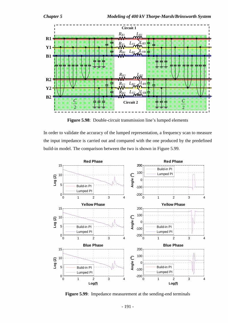
Chapter 5 Modeling of 400 kV Thorpe-Marsh/Brinsworth System
- 191 -
Figure 5.98: Double-circuit transmission line’s lumped elements
In order to validate the accuracy of the lumped representation, a frequency scan to measure
the input impedance is carried out and compared with the one produced by the predefined
build-in model. The comparison between the two is shown in Figure 5.99.
Figure 5.99: Impedance measurement at the sending-end terminals
R1
Y1
B1
R2
Y2
B2
RR1 LR1
RY1
RB1
RR2 LB2
RY2
RB2
Circuit 1
Circuit 2
2
C
2
C
LRY
LYB
LY1
LB1
LRY
LYB
LB2
LY2
0 1 2 3 40
5
10
15Red Phase
Log
(Z)
0 1 2 3 4-200
-100
0
100
200200Red Phase
Ang
le (
o)
0 1 2 3 40
5
10
15Yellow Phase
Log
(Z)
0 1 2 3 4-200
-100
0
100
200Yellow Phase
Ang
le (
o)
0 1 2 3 40
5
10
15Blue Phase
Log(f)
Log
(Z)
0 1 2 3 4-200
-100
0
100
200Blue Phase
Log(f)
Ang
le (
o)
Build-in PI
Lumped PI
Build-in PI
Lumped PI
Build-in PI
Lumped PI
Build-in PI
Lumped PI
Build-in PI
Lumped PI
Build-in PI
Lumped PI
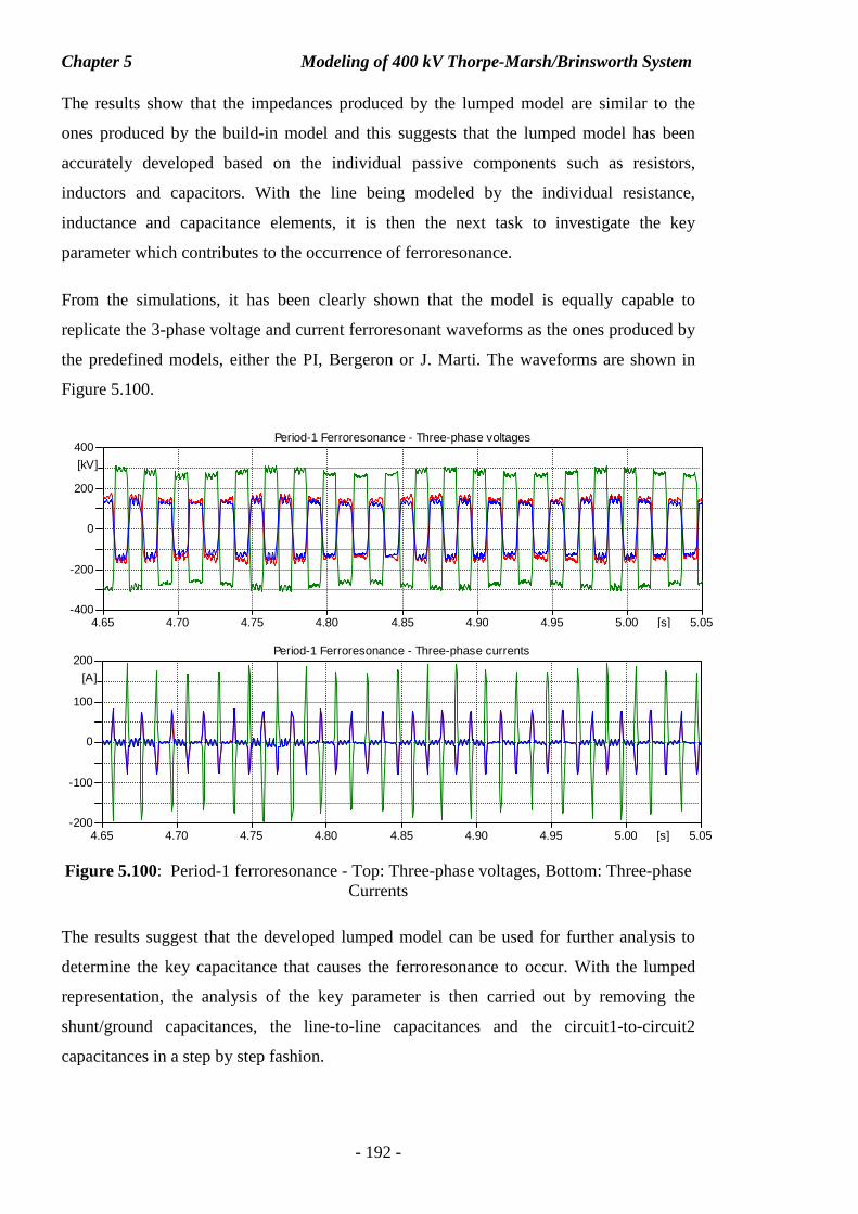
Chapter 5 Modeling of 400 kV Thorpe-Marsh/Brinsworth System
- 192 -
The results show that the impedances produced by the lumped model are similar to the
ones produced by the build-in model and this suggests that the lumped model has been
accurately developed based on the individual passive components such as resistors,
inductors and capacitors. With the line being modeled by the individual resistance,
inductance and capacitance elements, it is then the next task to investigate the key
parameter which contributes to the occurrence of ferroresonance.
From the simulations, it has been clearly shown that the model is equally capable to
replicate the 3-phase voltage and current ferroresonant waveforms as the ones produced by
the predefined models, either the PI, Bergeron or J. Marti. The waveforms are shown in
Figure 5.100.
Figure 5.100: Period-1 ferroresonance - Top: Three-phase voltages, Bottom: Three-phase Currents
The results suggest that the developed lumped model can be used for further analysis to
determine the key capacitance that causes the ferroresonance to occur. With the lumped
representation, the analysis of the key parameter is then carried out by removing the
shunt/ground capacitances, the line-to-line capacitances and the circuit1-to-circuit2
capacitances in a step by step fashion.
4.65 4.70 4.75 4.80 4.85 4.90 4.95 5.00 5.05[s]-400
-200
0
200
400
[kV]
Period-1 Ferroresonance - Three-phase voltages
4.65 4.70 4.75 4.80 4.85 4.90 4.95 5.00 5.05[s]-200
-100
0
100
200
[A]
Period-1 Ferroresonance - Three-phase currents
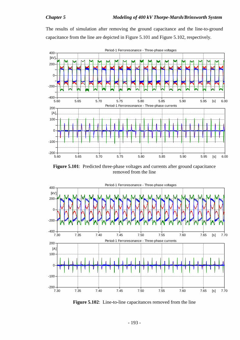
Chapter 5 Modeling of 400 kV Thorpe-Marsh/Brinsworth System
- 193 -
The results of simulation after removing the ground capacitance and the line-to-ground
capacitance from the line are depicted in Figure 5.101 and Figure 5.102, respectively.
Figure 5.101: Predicted three-phase voltages and currents after ground capacitance removed from the line
Figure 5.102: Line-to-line capacitances removed from the line
7.30 7.35 7.40 7.45 7.50 7.55 7.60 7.65 7.70[s]-400
-200
0
200
400
[kV]
Period-1 Ferroresonance - Three-phase voltages
7.30 7.35 7.40 7.45 7.50 7.55 7.60 7.65 7.70[s]-200
-100
0
100
200
[A]
Period-1 Ferroresonance - Three-phase currents
5.60 5.65 5.70 5.75 5.80 5.85 5.90 5.95 6.00[s]-400
-200
0
200
400
[kV]
Period-1 Ferroresonance - Three-phase voltages
5.60 5.65 5.70 5.75 5.80 5.85 5.90 5.95 6.00[s]-200
-100
0
100
200
[A]
Period-1 Ferroresonance - Three-phase currents
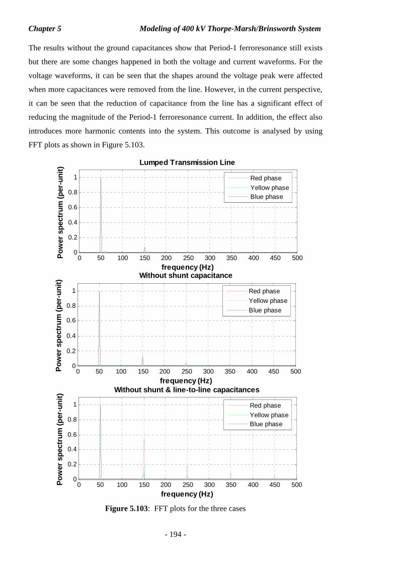
Chapter 5 Modeling of 400 kV Thorpe-Marsh/Brinsworth System
- 194 -
The results without the ground capacitances show that Period-1 ferroresonance still exists
but there are some changes happened in both the voltage and current waveforms. For the
voltage waveforms, it can be seen that the shapes around the voltage peak were affected
when more capacitances were removed from the line. However, in the current perspective,
it can be seen that the reduction of capacitance from the line has a significant effect of
reducing the magnitude of the Period-1 ferroresonance current. In addition, the effect also
introduces more harmonic contents into the system. This outcome is analysed by using
FFT plots as shown in Figure 5.103.
Figure 5.103: FFT plots for the three cases
0 50 100 150 200 250 300 350 400 450 5000
0.2
0.4
0.6
0.8
1
frequency (Hz)
Pow
er s
pect
rum
(pe
r-un
it)
Lumped Transmission Line
Red phase
Yellow phaseBlue phase
0 50 100 150 200 250 300 350 400 450 5000
0.2
0.4
0.6
0.8
1
frequency (Hz)
Pow
er s
pect
rum
(pe
r-un
it)
Without shunt capacitance
Red phase
Yellow phase
Blue phase
0 50 100 150 200 250 300 350 400 450 5000
0.2
0.4
0.6
0.8
1
frequency (Hz)
Pow
er s
pect
rum
(pe
r-un
it)
Without shunt & line-to-line capacitances
Red phase
Yellow phaseBlue phase
Chapter 5 Modeling of 400 kV Thorpe-Marsh/Brinsworth System
- 195 -
Figure 5.103 shows that the line without the presence of the shunt and line-to-line
capacitances has the influence of introducing harmonics into the system.
From the investigation, it has been found that each of the coupling capacitances of the line
play an important role as a key parameter for the occurrence of Period-1 ferroresonance.
Without the shunt and the line-to-line capacitances taking part in the line, the arrangement
of the circuit-to-circuit capacitances are actually connected in series with the transformer.
This study showed that the series arrangement of the capacitances and the transformer
serve as a purpose of sustaining the amplitude of the three-phase voltages and currents. On
the other hand, the studies without the shunt and the line-to-line capacitances has shown
that there is a dramatic effect of reducing the amplitude of the ferroresonance currents, and
this suggests that both of them are actually contributing to the current boosting of the
phenomenon.
5.8 Summary
The simulations involved in all the six case studies using both the BCTRAN+ and
HYBRID transformer models combined with either PI, Bergeron or Marti transmission line
model have been carried out. Out of all the six combinations of the simulation models have
been developed, and the comparisons between the simulations and the field recording
results draw the following observations;
(1) A great deal of simulation attempts are required in order to reproduce the types of
ferroresonance responses (Period-1 and Period-3) by the simulation models. The
reason is because of the initial condition of the three-voltage waves after the current
interruption are not repeatable from one cycle to another cycle.
(2) Degree of saturation for the transformer core was chosen as n = 27 because the
simulation results are comparable with the field recording waveforms.
(3) There is not single simulation model, out of the six models developed, can be regarded
as the best. All of them are comparable and are equally capable to replicate both the
Period-1 and Period-3 ferroresonance waveforms. However, the limitations of these
models are that they are not able to match the current magnitudes of the red and blue
phases of the Period-1 ferroresonance and also the three-phase currents of the Period-3

Chapter 5 Modeling of 400 kV Thorpe-Marsh/Brinsworth System
- 196 -
ferroresonance. In addition, there is no high frequency ripples appearing on both the 3-
phase voltages and currents.
(4) All the six simulation models can be employed for the study of ferroresonance but one
particular model i.e. modeling the transformer using HYBRID and the transmission
line in PI has been preferred.
(5) The preferred model is then further improved by modifying the core characteristic and
the improved model is able to provide the high frequency ripples on the three-phase
voltage and current waveforms for only the Period-3 ferroresonance. In addition to
that, the magnitude of the yellow phase current has been drastically manifested.
(6) Discrepancy between recorded and predicted current still exists for Red and Blue
phases. One of the possible reasons could be due to the core characteristic used to
model the transformer is not fully representative to account for the flux distribution
into airgap and its fringing effect, particularly, in the case of deep saturation.
However, the shapes (see waveform figures) match quite well between the simulation
and the field recording waveforms.
The observations on the key parameters that would influence the occurrence of the Period-
1 ferroresonance are explained as follows:
(1) Both the transformer’s coupling capacitances and the cable capacitance do not provide
any significant influence on the occurrence of the Period-1 ferroresonance.
(2) From the investigation, all the coupling capacitances of the line have contributed
individually to the occurrence of the phenomenon. The role of the circuit-to-circuit
capacitances is to provide the sustainable amplitude of the ferroresonance while the
rest provides the additional energy transfers from the line to the saturable core
inductance.
Chapter 6 Modeling of 400 kV Iron-Acton/Melksham System
- 197 -
CHAPTER 6 CHAPTER 6 CHAPTER 6 CHAPTER 6
666... MMM OOODDDEEELLL III NNNGGG OOOFFF 444000000 KKK VVV III RRROOONNN---AAACCCTTTOOONNN///MMM EEELLL KKK SSSHHHAAAMMM SSSYYYSSSTTTEEEMMM
6.1 Introduction
In the preceding chapter, modeling of power system components to represent a 400 kV
transmission system was carried out. The simulation model which has been developed is
able to reproduce both the Period-1 and Period-3 ferroresonance waveforms in good
agreement with the field test recording waveforms.
The aim of this chapter is to carry out a case study on a particular circuit configuration,
regarding the likelihood of occurrence of sustained fundamental frequency (Period-1)
ferroresonance. The study considered a complex arrangement including a mesh corner
substation connected by overhead lines to a transformer feeder. The assessment upon the
circuit is carried out by simulation studies using the ATPDraw. Since there are no field
recording waveforms available for comparative verification, modeling of the individual
components to represent the system are based of the criteria that have been obtained
previously.
In addition to evaluating the system, this chapter also investigates the effectiveness of
mitigation measure to quench the intended ferroresonance by switching-in a 60 MVAR
shunt reactor which is connected at the 13 kV tertiary winding.
Furthermore, a sensitivity study on transmission line length is also carried out with an aim
to find out the likelihood of occurrence of ferroresonance.
6.2 Description of the Transmission System
Figure 6.1 shows the single-line arrangement of one of the circuits on the National Grid
transmission systems. The circuit arrangement which is believed to have a potential risk of
inducing the Period-1 ferroresonance consists of a 33 km long double-circuit transmission
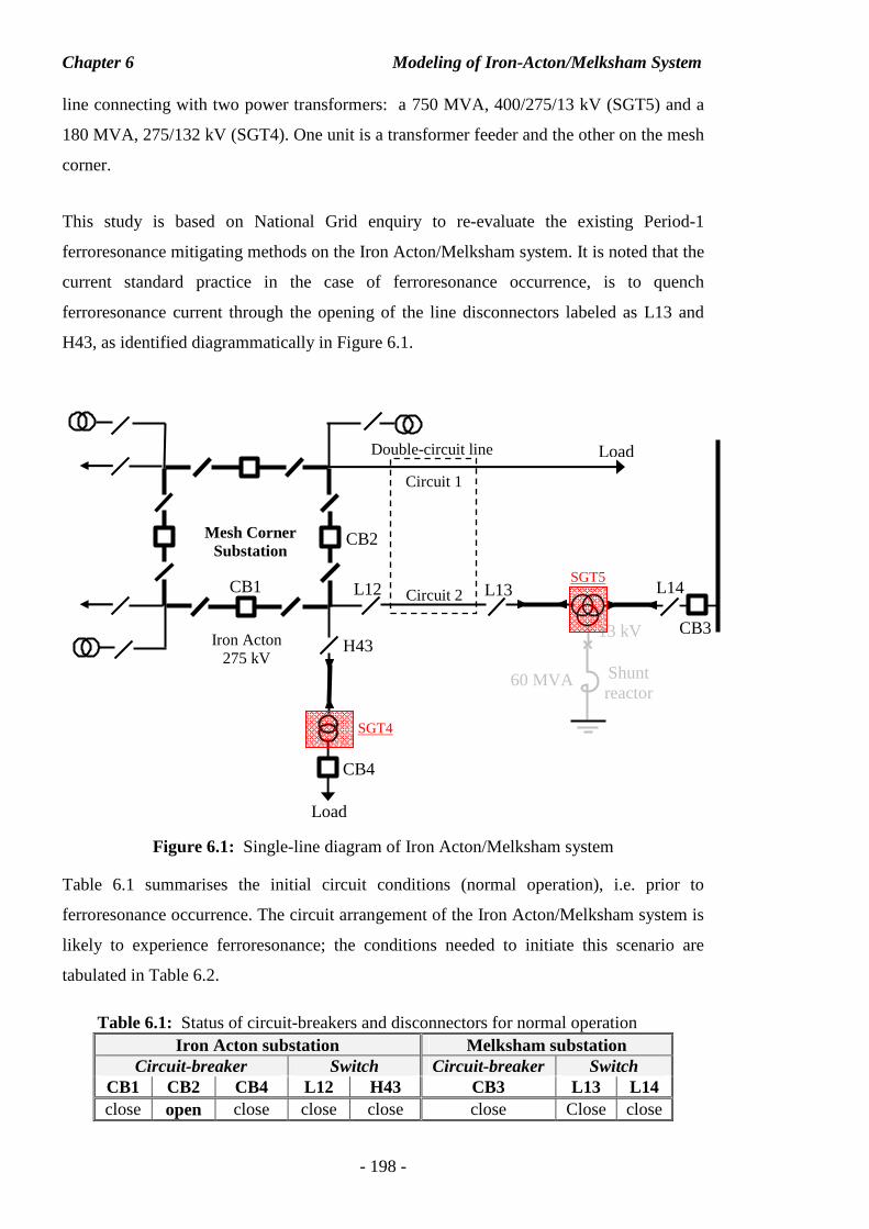
Chapter 6 Modeling of Iron-Acton/Melksham System
- 198 -
line connecting with two power transformers: a 750 MVA, 400/275/13 kV (SGT5) and a
180 MVA, 275/132 kV (SGT4). One unit is a transformer feeder and the other on the mesh
corner.
This study is based on National Grid enquiry to re-evaluate the existing Period-1
ferroresonance mitigating methods on the Iron Acton/Melksham system. It is noted that the
current standard practice in the case of ferroresonance occurrence, is to quench
ferroresonance current through the opening of the line disconnectors labeled as L13 and
H43, as identified diagrammatically in Figure 6.1.
Figure 6.1: Single-line diagram of Iron Acton/Melksham system
Table 6.1 summarises the initial circuit conditions (normal operation), i.e. prior to
ferroresonance occurrence. The circuit arrangement of the Iron Acton/Melksham system is
likely to experience ferroresonance; the conditions needed to initiate this scenario are
tabulated in Table 6.2.
Table 6.1: Status of circuit-breakers and disconnectors for normal operation Iron Acton substation Melksham substation
Circuit-breaker Switch Circuit-breaker Switch CB1 CB2 CB4 L12 H43 CB3 L13 L14 close open close close close close Close close
13 kV
Shunt reactor
60 MVA
H43 CB3
CB1
CB2
L12
Load
Iron Acton 275 kV
Mesh Corner Substation
Double-circuit line
Circuit 1
Circuit 2
Load
CB4
SGT4
L13 L14 SGT5
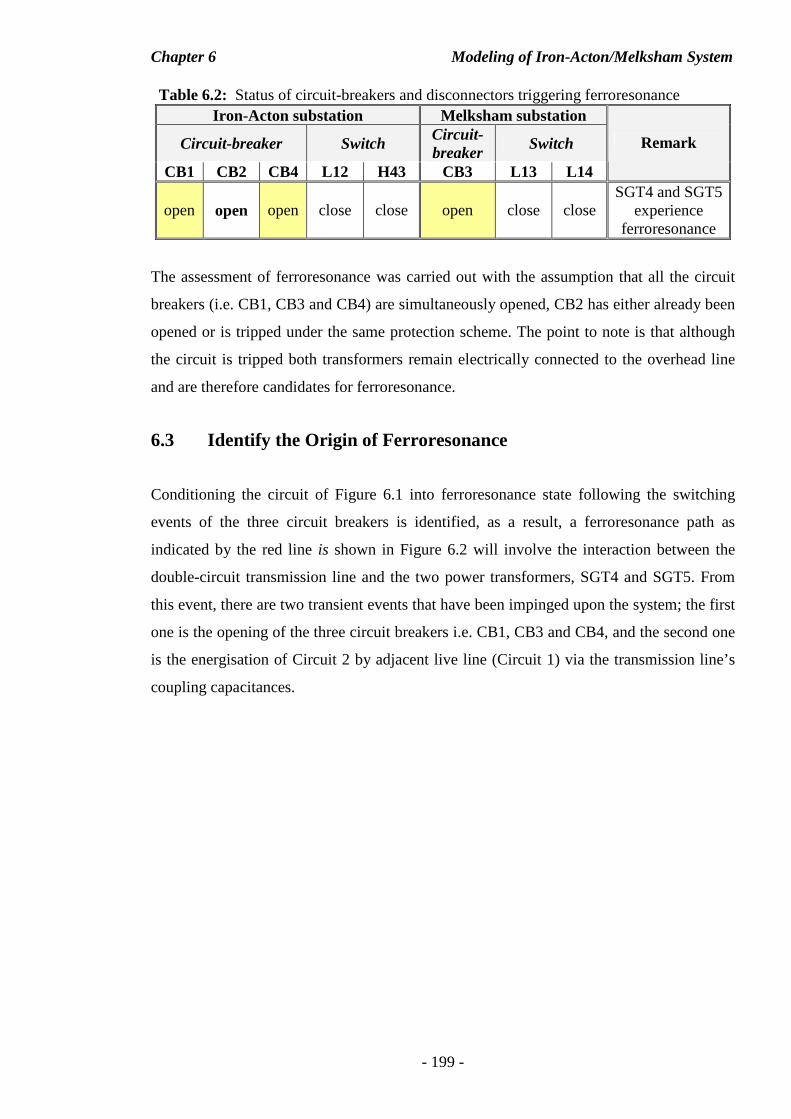
Chapter 6 Modeling of Iron-Acton/Melksham System
- 199 -
Table 6.2: Status of circuit-breakers and disconnectors triggering ferroresonance Iron-Acton substation Melksham substation
Circuit-breaker Switch Circuit-breaker
Switch
CB1 CB2 CB4 L12 H43 CB3 L13 L14
Remark
open open open close close open close close SGT4 and SGT5
experience ferroresonance
The assessment of ferroresonance was carried out with the assumption that all the circuit
breakers (i.e. CB1, CB3 and CB4) are simultaneously opened, CB2 has either already been
opened or is tripped under the same protection scheme. The point to note is that although
the circuit is tripped both transformers remain electrically connected to the overhead line
and are therefore candidates for ferroresonance.
6.3 Identify the Origin of Ferroresonance
Conditioning the circuit of Figure 6.1 into ferroresonance state following the switching
events of the three circuit breakers is identified, as a result, a ferroresonance path as
indicated by the red line is shown in Figure 6.2 will involve the interaction between the
double-circuit transmission line and the two power transformers, SGT4 and SGT5. From
this event, there are two transient events that have been impinged upon the system; the first
one is the opening of the three circuit breakers i.e. CB1, CB3 and CB4, and the second one
is the energisation of Circuit 2 by adjacent live line (Circuit 1) via the transmission line’s
coupling capacitances.
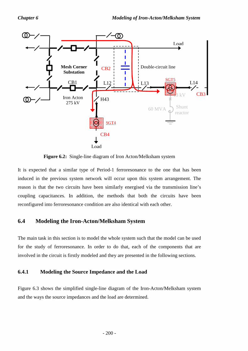
Chapter 6 Modeling of Iron-Acton/Melksham System
- 200 -
Figure 6.2: Single-line diagram of Iron Acton/Melksham system
It is expected that a similar type of Period-1 ferroresonance to the one that has been
induced in the previous system network will occur upon this system arrangement. The
reason is that the two circuits have been similarly energised via the transmission line’s
coupling capacitances. In addition, the methods that both the circuits have been
reconfigured into ferroresonance condition are also identical with each other.
6.4 Modeling the Iron-Acton/Melksham System
The main task in this section is to model the whole system such that the model can be used
for the study of ferroresonance. In order to do that, each of the components that are
involved in the circuit is firstly modeled and they are presented in the following sections.
6.4.1 Modeling the Source Impedance and the Load
Figure 6.3 shows the simplified single-line diagram of the Iron-Acton/Melksham system
and the ways the source impedances and the load are determined.
13 kV
Shunt reactor
60 MVA
H43 CB3
CB1
CB2
L12
Load
Iron Acton 275 kV
Mesh Corner Substation
Double-circuit line
Load
SGT4
L13 L14 SGT5
CB4
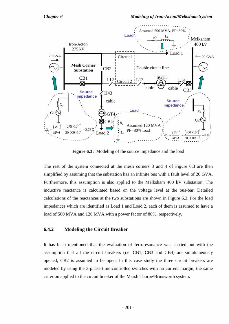
Chapter 6 Modeling of Iron-Acton/Melksham System
- 201 -
Figure 6.3: Modeling of the source impedance and the load
The rest of the system connected at the mesh corners 3 and 4 of Figure 6.3 are then
simplified by assuming that the substation has an infinite bus with a fault level of 20 GVA.
Furthermore, this assumption is also applied to the Melksham 400 kV substation. The
inductive reactance is calculated based on the voltage level at the bus-bar. Detailed
calculations of the reactances at the two substations are shown in Figure 6.3. For the load
impedances which are identified as Load 1 and Load 2, each of them is assumed to have a
load of 500 MVA and 120 MVA with a power factor of 80%, respectively.
6.4.2 Modeling the Circuit Breaker
It has been mentioned that the evaluation of ferroresonance was carried out with the
assumption that all the circuit breakers (i.e. CB1, CB3 and CB4) are simultaneously
opened, CB2 is assumed to be open. In this case study the three circuit breakers are
modeled by using the 3-phase time-controlled switches with no current margin, the same
criterion applied to the circuit breaker of the Marsh Thorpe/Brinsworth system.
H43 CB3
CB1
CB2
L12
Load 1
SGT5
Iron-Acton 275 kV
Mesh Corner Substation Double circuit line
Circuit 1
Circuit 2
Load 2
CB4
SGT4
L13 L14
Melksham 400 kV
20 GVA 20 GVA
R1 L1
Assumed 500 MVA, PF=80% Load
X2
G2
( ) ( )22 3
2 6
400 108
20,000 10
kVX
MVA
×= = = Ω
×
R2
L2
Assumed 120 MVA PF=80% load
Load G1
X1
( ) ( )22 3
1 6
275 103.78
20,000 10
kVX
MVA
×= = = Ω
×
Source impedance
Source impedance
cable cable
cable
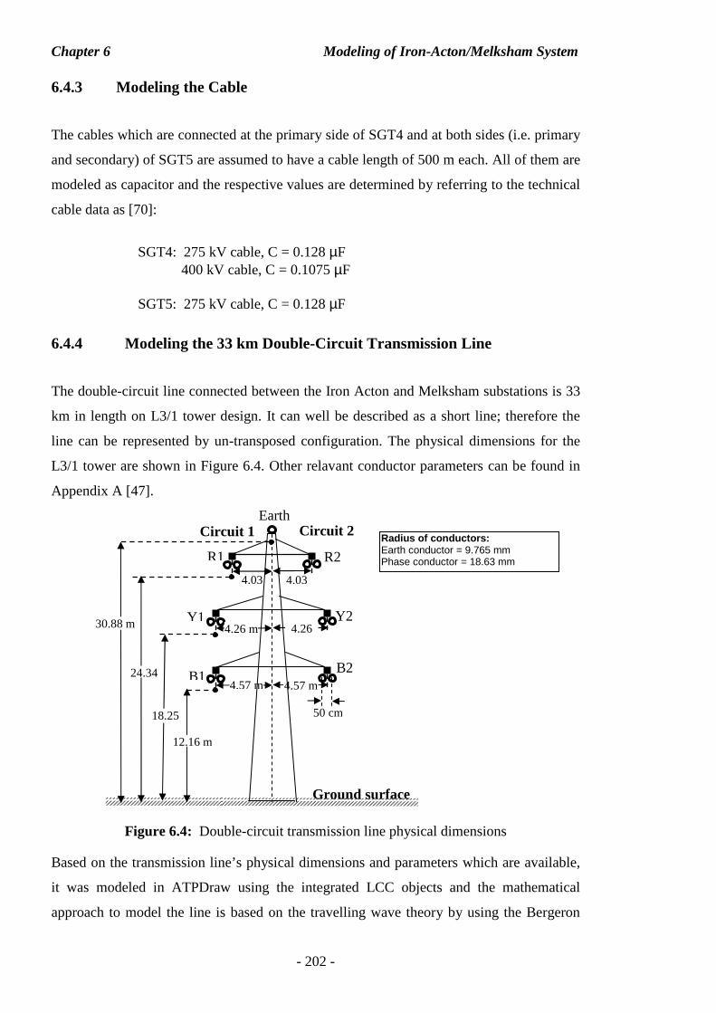
Chapter 6 Modeling of Iron-Acton/Melksham System
- 202 -
6.4.3 Modeling the Cable
The cables which are connected at the primary side of SGT4 and at both sides (i.e. primary
and secondary) of SGT5 are assumed to have a cable length of 500 m each. All of them are
modeled as capacitor and the respective values are determined by referring to the technical
cable data as [70]:
SGT4: 275 kV cable, C = 0.128 µF
400 kV cable, C = 0.1075 µF
SGT5: 275 kV cable, C = 0.128 µF
6.4.4 Modeling the 33 km Double-Circuit Transmission Line
The double-circuit line connected between the Iron Acton and Melksham substations is 33
km in length on L3/1 tower design. It can well be described as a short line; therefore the
line can be represented by un-transposed configuration. The physical dimensions for the
L3/1 tower are shown in Figure 6.4. Other relavant conductor parameters can be found in
Appendix A [47].
Figure 6.4: Double-circuit transmission line physical dimensions
Based on the transmission line’s physical dimensions and parameters which are available,
it was modeled in ATPDraw using the integrated LCC objects and the mathematical
approach to model the line is based on the travelling wave theory by using the Bergeron
Earth
Ground surface
12.16 m
18.25 m
24.34
30.88 m
R1 R2
4.03 4.03
Y1 Y2 4.26 m 4.26
B1 B2
4.57 m 4.57 m
50 cm
Circuit 1 Circuit 2 Radius of conductors: Earth conductor = 9.765 mm Phase conductor = 18.63 mm
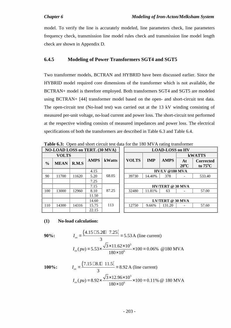
Chapter 6 Modeling of Iron-Acton/Melksham System
- 203 -
model. To verify the line is accurately modeled, line parameters check, line parameters
frequency check, transmission line model rules check and transmission line model length
check are shown in Appendix D.
6.4.5 Modeling of Power Transformers SGT4 and SGT5
Two transformer models, BCTRAN and HYBRID have been discussed earlier. Since the
HYBRID model required core dimensions of the transformer which is not available, the
BCTRAN+ model is therefore employed. Both transformers SGT4 and SGT5 are modeled
using BCTRAN+ [44] transformer model based on the open- and short-circuit test data.
The open-circuit test (No-load test) was carried out at the 13 kV winding consisting of
measured per-unit voltage, no-load current and power loss. The short-circuit test performed
at the respective winding consists of measured impedances and power loss. The electrical
specifications of both the transformers are described in Table 6.3 and Table 6.4.
Table 6.3: Open and short circuit test data for the 180 MVA rating transformer NO-LOAD LOSS on TERT. (30 MVA) LOAD-LOSS on HV
VOLTS kWATTS
% MEAN R.M.S AMPS kWatts VOLTS IMP AMPS At
20oC Corrected
to 75oC 4.15 HV/LV @180 MVA
90 11700 11620 5.20 39730 14.40% 378 - 533.40 7.25
68.05
7.15 HV/TERT @ 30 MVA
100 13000 12960 8.10 32480 11.81% 63 - 57.00 11.50
87.25
14.60 LV/TERT @ 30 MVA 110 14300 14316 15.75 12750 9.66% 131.20 - 57.60
22.15 113
(1) No-load calculation:
90%: ( )4.15 5.20 7.25
5.533exI
+ += = A (line current)
3
6
3 11.62 10( ) 5.53 100 0.06%
180 10exI pu× ×= × × =
× @180 MVA
100%: ( )7.15 8.1 11.5
8.923exI
+ += = A (line current)
3
6
3 12.96 10( ) 8.92 100 0.11%
180 10exI pu× ×= × × =
×@ 180 MVA
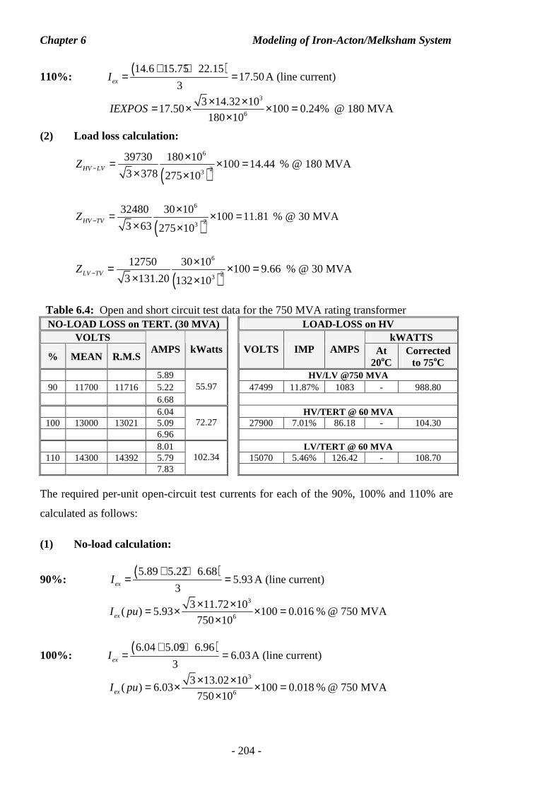
Chapter 6 Modeling of Iron-Acton/Melksham System
- 204 -
110%: ( )14.6 15.75 22.15
17.503exI
+ += = A (line current)
3
6
3 14.32 1017.50 100 0.24%
180 10IEXPOS
× ×= × × =×
@ 180 MVA
(2) Load loss calculation:
( )6
23
39730 180 10100 14.44
3 378 275 10HV LVZ −
×= × =× ×
% @ 180 MVA
( )6
23
32480 30 10100 11.81
3 63 275 10HV TVZ −
×= × =× ×
% @ 30 MVA
( )6
23
12750 30 10100 9.66
3 131.20 132 10LV TVZ −
×= × =× ×
% @ 30 MVA
Table 6.4: Open and short circuit test data for the 750 MVA rating transformer NO-LOAD LOSS on TERT. (30 MVA) LOAD-LOSS on HV
VOLTS kWATTS
% MEAN R.M.S AMPS kWatts VOLTS IMP AMPS At
20oC Corrected
to 75oC 5.89 HV/LV @750 MVA
90 11700 11716 5.22 47499 11.87% 1083 - 988.80 6.68
55.97
6.04 HV/TERT @ 60 MVA
100 13000 13021 5.09 27900 7.01% 86.18 - 104.30 6.96
72.27
8.01 LV/TERT @ 60 MVA 110 14300 14392 5.79 15070 5.46% 126.42 - 108.70
7.83 102.34
The required per-unit open-circuit test currents for each of the 90%, 100% and 110% are
calculated as follows:
(1) No-load calculation:
90%: ( )5.89 5.22 6.68
5.933exI
+ += = A (line current)
3
6
3 11.72 10( ) 5.93 100 0.016 %
750 10exI pu× ×= × × =
×@ 750 MVA
100%: ( )6.04 5.09 6.96
6.033exI
+ += = A (line current)
3
6
3 13.02 10( ) 6.03 100 0.018 %
750 10exI pu× ×= × × =
×@ 750 MVA
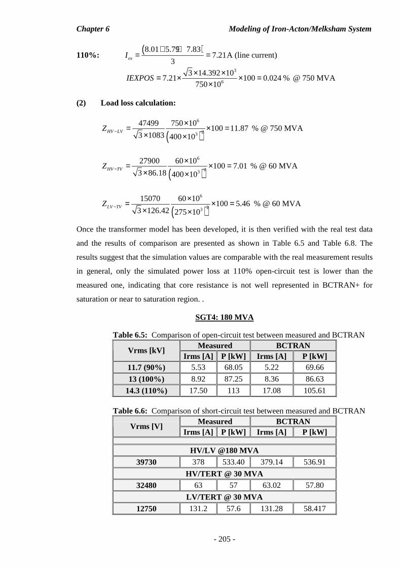
Chapter 6 Modeling of Iron-Acton/Melksham System
- 205 -
110%: ( )8.01 5.79 7.83
7.213exI
+ += = A (line current)
3
6
3 14.392 107.21 100 0.024 %
750 10IEXPOS
× ×= × × =×
@ 750 MVA
(2) Load loss calculation:
( )6
23
47499 750 10100 11.87
3 1083 400 10HV LVZ −
×= × =× ×
% @ 750 MVA
( )6
23
27900 60 10100 7.01
3 86.18 400 10HV TVZ −
×= × =× ×
% @ 60 MVA
( )6
23
15070 60 10100 5.46
3 126.42 275 10LV TVZ −
×= × =× ×
% @ 60 MVA
Once the transformer model has been developed, it is then verified with the real test data
and the results of comparison are presented as shown in Table 6.5 and Table 6.8. The
results suggest that the simulation values are comparable with the real measurement results
in general, only the simulated power loss at 110% open-circuit test is lower than the
measured one, indicating that core resistance is not well represented in BCTRAN+ for
saturation or near to saturation region. .
SGT4: 180 MVA
Table 6.5: Comparison of open-circuit test between measured and BCTRAN Measured BCTRAN
Vrms [kV] Irms [A] P [kW] Irms [A] P [kW]
11.7 (90%) 5.53 68.05 5.22 69.66
13 (100%) 8.92 87.25 8.36 86.63
14.3 (110%) 17.50 113 17.08 105.61
Table 6.6: Comparison of short-circuit test between measured and BCTRAN Measured BCTRAN
Vrms [V] Irms [A] P [kW] Irms [A] P [kW]
HV/LV @180 MVA 39730 378 533.40 379.14 536.91
HV/TERT @ 30 MVA 32480 63 57 63.02 57.80
LV/TERT @ 30 MVA 12750 131.2 57.6 131.28 58.417
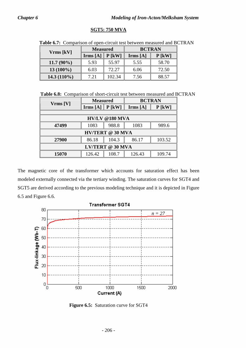
Chapter 6 Modeling of Iron-Acton/Melksham System
- 206 -
SGT5: 750 MVA
Table 6.7: Comparison of open-circuit test between measured and BCTRAN Measured BCTRAN
Vrms [kV] Irms [A] P [kW] Irms [A] P [kW]
11.7 (90%) 5.93 55.97 5.55 58.70
13 (100%) 6.03 72.27 6.06 72.50
14.3 (110%) 7.21 102.34 7.56 88.57
Table 6.8: Comparison of short-circuit test between measured and BCTRAN Measured BCTRAN
Vrms [V] Irms [A] P [kW] Irms [A] P [kW]
HV/LV @180 MVA 47499 1083 988.8 1083 989.6
HV/TERT @ 30 MVA 27900 86.18 104.3 86.17 103.52
LV/TERT @ 30 MVA 15070 126.42 108.7 126.43 109.74
The magnetic core of the transformer which accounts for saturation effect has been
modeled externally connected via the tertiary winding. The saturation curves for SGT4 and
SGT5 are derived according to the previous modeling technique and it is depicted in Figure
6.5 and Figure 6.6.
Figure 6.5: Saturation curve for SGT4
n = 27
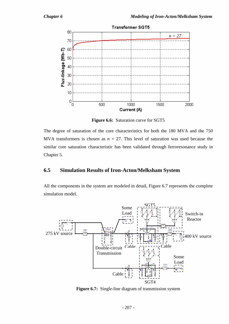
Chapter 6 Modeling of Iron-Acton/Melksham System
- 207 -
Figure 6.6: Saturation curve for SGT5
The degree of saturation of the core characteristics for both the 180 MVA and the 750
MVA transformers is chosen as n = 27. This level of saturation was used because the
similar core saturation characteristic has been validated through ferroresonance study in
Chapter 5.
6.5 Simulation Results of Iron-Acton/Melksham System
All the components in the system are modeled in detail, Figure 6.7 represents the complete
simulation model.
Figure 6.7: Single-line diagram of transmission system
n = 27
SGT5 Some Load
400 kV source 275 kV source
Cable
Cable
Double-circuit Transmission
line
Cable
SGT4
Some Load
Switch-in Reactor
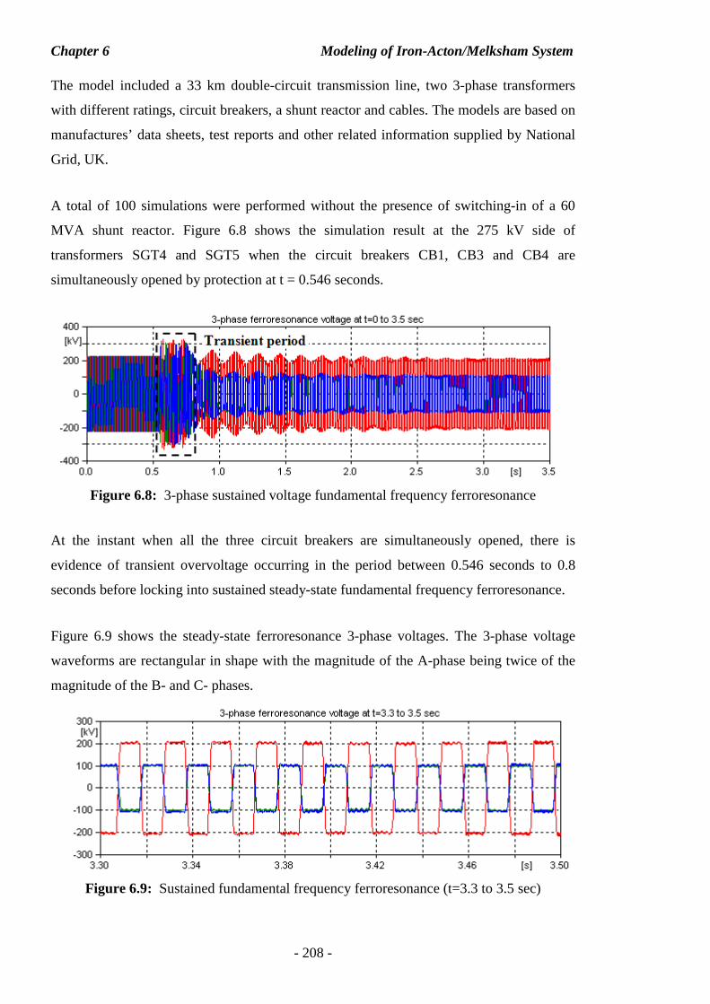
Chapter 6 Modeling of Iron-Acton/Melksham System
- 208 -
The model included a 33 km double-circuit transmission line, two 3-phase transformers
with different ratings, circuit breakers, a shunt reactor and cables. The models are based on
manufactures’ data sheets, test reports and other related information supplied by National
Grid, UK.
A total of 100 simulations were performed without the presence of switching-in of a 60
MVA shunt reactor. Figure 6.8 shows the simulation result at the 275 kV side of
transformers SGT4 and SGT5 when the circuit breakers CB1, CB3 and CB4 are
simultaneously opened by protection at t = 0.546 seconds.
Figure 6.8: 3-phase sustained voltage fundamental frequency ferroresonance
At the instant when all the three circuit breakers are simultaneously opened, there is
evidence of transient overvoltage occurring in the period between 0.546 seconds to 0.8
seconds before locking into sustained steady-state fundamental frequency ferroresonance.
Figure 6.9 shows the steady-state ferroresonance 3-phase voltages. The 3-phase voltage
waveforms are rectangular in shape with the magnitude of the A-phase being twice of the
magnitude of the B- and C- phases.
Figure 6.9: Sustained fundamental frequency ferroresonance (t=3.3 to 3.5 sec)
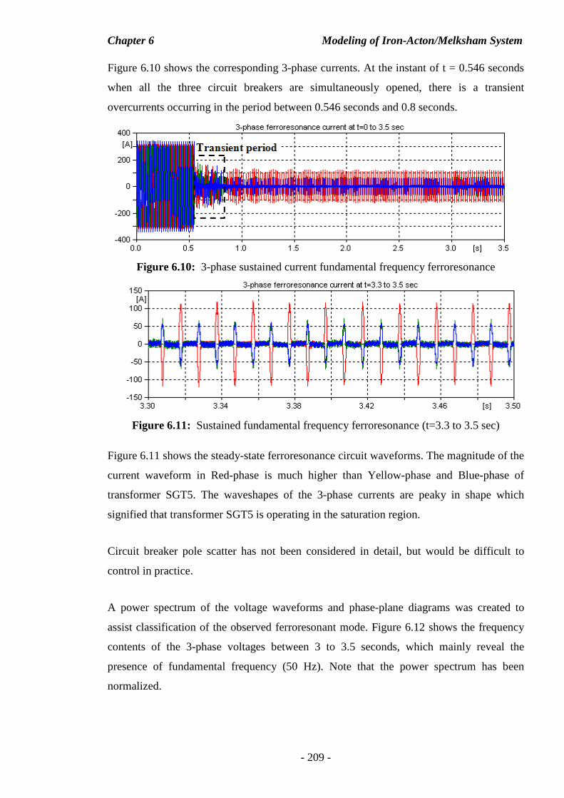
Chapter 6 Modeling of Iron-Acton/Melksham System
- 209 -
Figure 6.10 shows the corresponding 3-phase currents. At the instant of t = 0.546 seconds
when all the three circuit breakers are simultaneously opened, there is a transient
overcurrents occurring in the period between 0.546 seconds and 0.8 seconds.
Figure 6.10: 3-phase sustained current fundamental frequency ferroresonance
Figure 6.11: Sustained fundamental frequency ferroresonance (t=3.3 to 3.5 sec)
Figure 6.11 shows the steady-state ferroresonance circuit waveforms. The magnitude of the
current waveform in Red-phase is much higher than Yellow-phase and Blue-phase of
transformer SGT5. The waveshapes of the 3-phase currents are peaky in shape which
signified that transformer SGT5 is operating in the saturation region.
Circuit breaker pole scatter has not been considered in detail, but would be difficult to
control in practice.
A power spectrum of the voltage waveforms and phase-plane diagrams was created to
assist classification of the observed ferroresonant mode. Figure 6.12 shows the frequency
contents of the 3-phase voltages between 3 to 3.5 seconds, which mainly reveal the
presence of fundamental frequency (50 Hz). Note that the power spectrum has been
normalized.
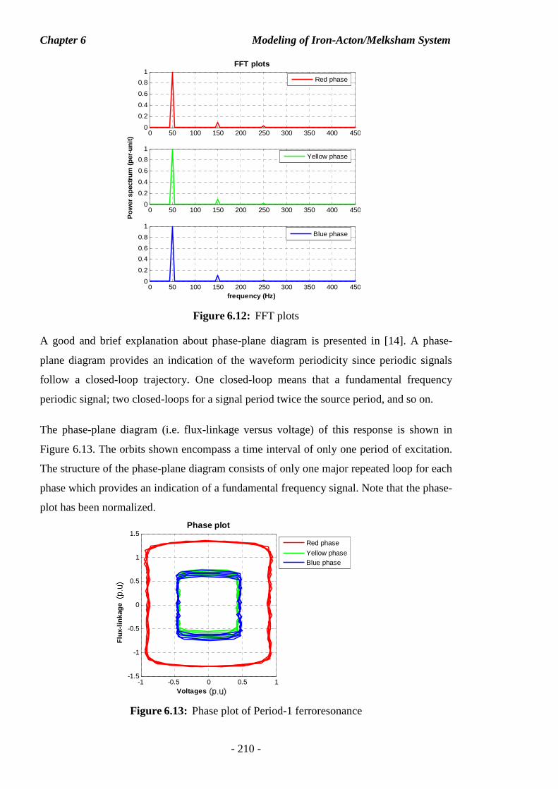
Chapter 6 Modeling of Iron-Acton/Melksham System
- 210 -
Figure 6.12: FFT plots
A good and brief explanation about phase-plane diagram is presented in [14]. A phase-
plane diagram provides an indication of the waveform periodicity since periodic signals
follow a closed-loop trajectory. One closed-loop means that a fundamental frequency
periodic signal; two closed-loops for a signal period twice the source period, and so on.
The phase-plane diagram (i.e. flux-linkage versus voltage) of this response is shown in
Figure 6.13. The orbits shown encompass a time interval of only one period of excitation.
The structure of the phase-plane diagram consists of only one major repeated loop for each
phase which provides an indication of a fundamental frequency signal. Note that the phase-
plot has been normalized.
Figure 6.13: Phase plot of Period-1 ferroresonance
0 50 100 150 200 250 300 350 400 4500
0.2
0.4
0.6
0.8
1FFT plots
0 50 100 150 200 250 300 350 400 4500
0.2
0.4
0.6
0.8
1
Pow
er s
pect
rum
(pe
r-un
it)
0 50 100 150 200 250 300 350 400 4500
0.2
0.4
0.6
0.8
1
frequency (Hz)
Red phase
Yellow phase
Blue phase
-1 -0.5 0 0.5 1-1.5
-1
-0.5
0
0.5
1
1.5
Voltages (Per-unit)
Flu
x-lin
kage
(P
er-U
nit)
Phase plot
Red phase
Yellow phaseBlue phase
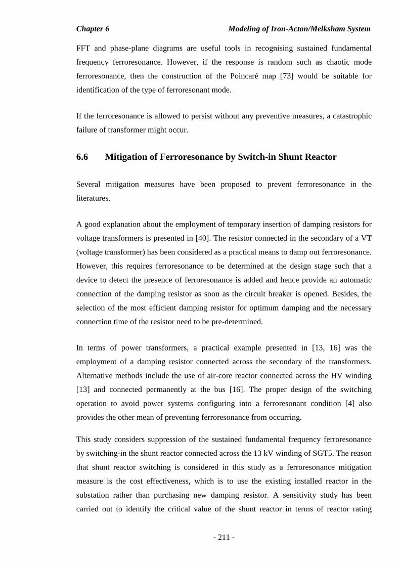
Chapter 6 Modeling of Iron-Acton/Melksham System
- 211 -
FFT and phase-plane diagrams are useful tools in recognising sustained fundamental
frequency ferroresonance. However, if the response is random such as chaotic mode
ferroresonance, then the construction of the Poincaré map [73] would be suitable for
identification of the type of ferroresonant mode.
If the ferroresonance is allowed to persist without any preventive measures, a catastrophic
failure of transformer might occur.
6.6 Mitigation of Ferroresonance by Switch-in Shunt Reactor
Several mitigation measures have been proposed to prevent ferroresonance in the
literatures.
A good explanation about the employment of temporary insertion of damping resistors for
voltage transformers is presented in [40]. The resistor connected in the secondary of a VT
(voltage transformer) has been considered as a practical means to damp out ferroresonance.
However, this requires ferroresonance to be determined at the design stage such that a
device to detect the presence of ferroresonance is added and hence provide an automatic
connection of the damping resistor as soon as the circuit breaker is opened. Besides, the
selection of the most efficient damping resistor for optimum damping and the necessary
connection time of the resistor need to be pre-determined.
In terms of power transformers, a practical example presented in [13, 16] was the
employment of a damping resistor connected across the secondary of the transformers.
Alternative methods include the use of air-core reactor connected across the HV winding
[13] and connected permanently at the bus [16]. The proper design of the switching
operation to avoid power systems configuring into a ferroresonant condition [4] also
provides the other mean of preventing ferroresonance from occurring.
This study considers suppression of the sustained fundamental frequency ferroresonance
by switching-in the shunt reactor connected across the 13 kV winding of SGT5. The reason
that shunt reactor switching is considered in this study as a ferroresonance mitigation
measure is the cost effectiveness, which is to use the existing installed reactor in the
substation rather than purchasing new damping resistor. A sensitivity study has been
carried out to identify the critical value of the shunt reactor in terms of reactor rating
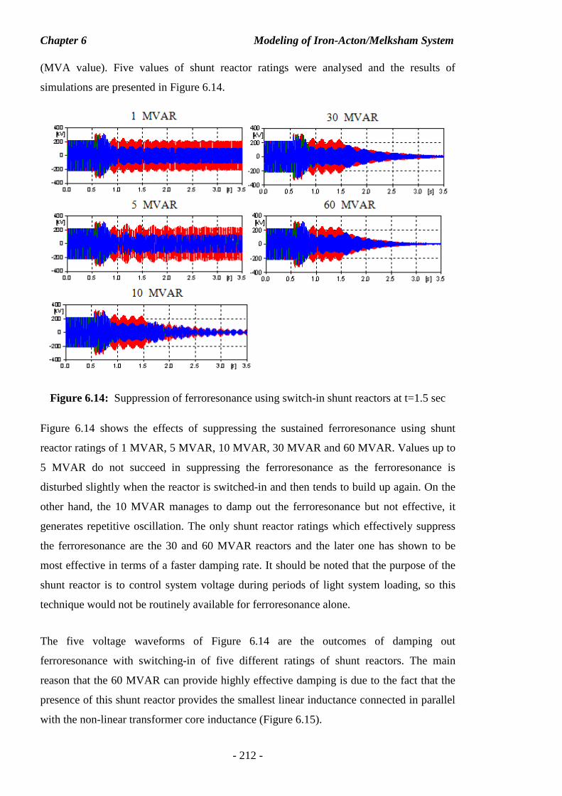
Chapter 6 Modeling of Iron-Acton/Melksham System
- 212 -
(MVA value). Five values of shunt reactor ratings were analysed and the results of
simulations are presented in Figure 6.14.
Figure 6.14: Suppression of ferroresonance using switch-in shunt reactors at t=1.5 sec
Figure 6.14 shows the effects of suppressing the sustained ferroresonance using shunt
reactor ratings of 1 MVAR, 5 MVAR, 10 MVAR, 30 MVAR and 60 MVAR. Values up to
5 MVAR do not succeed in suppressing the ferroresonance as the ferroresonance is
disturbed slightly when the reactor is switched-in and then tends to build up again. On the
other hand, the 10 MVAR manages to damp out the ferroresonance but not effective, it
generates repetitive oscillation. The only shunt reactor ratings which effectively suppress
the ferroresonance are the 30 and 60 MVAR reactors and the later one has shown to be
most effective in terms of a faster damping rate. It should be noted that the purpose of the
shunt reactor is to control system voltage during periods of light system loading, so this
technique would not be routinely available for ferroresonance alone.
The five voltage waveforms of Figure 6.14 are the outcomes of damping out
ferroresonance with switching-in of five different ratings of shunt reactors. The main
reason that the 60 MVAR can provide highly effective damping is due to the fact that the
presence of this shunt reactor provides the smallest linear inductance connected in parallel
with the non-linear transformer core inductance (Figure 6.15).
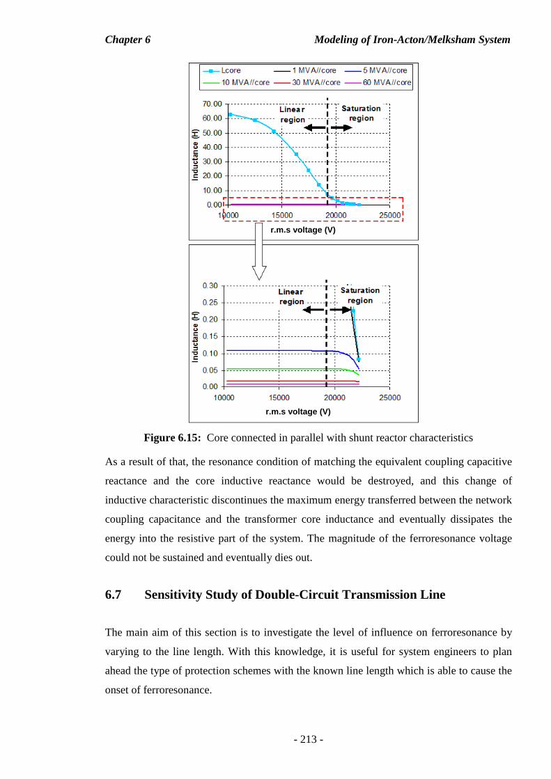
Chapter 6 Modeling of Iron-Acton/Melksham System
- 213 -
Figure 6.15: Core connected in parallel with shunt reactor characteristics
As a result of that, the resonance condition of matching the equivalent coupling capacitive
reactance and the core inductive reactance would be destroyed, and this change of
inductive characteristic discontinues the maximum energy transferred between the network
coupling capacitance and the transformer core inductance and eventually dissipates the
energy into the resistive part of the system. The magnitude of the ferroresonance voltage
could not be sustained and eventually dies out.
6.7 Sensitivity Study of Double-Circuit Transmission Line
The main aim of this section is to investigate the level of influence on ferroresonance by
varying to the line length. With this knowledge, it is useful for system engineers to plan
ahead the type of protection schemes with the known line length which is able to cause the
onset of ferroresonance.
r.m.s voltage (V)
r.m.s voltage (V)
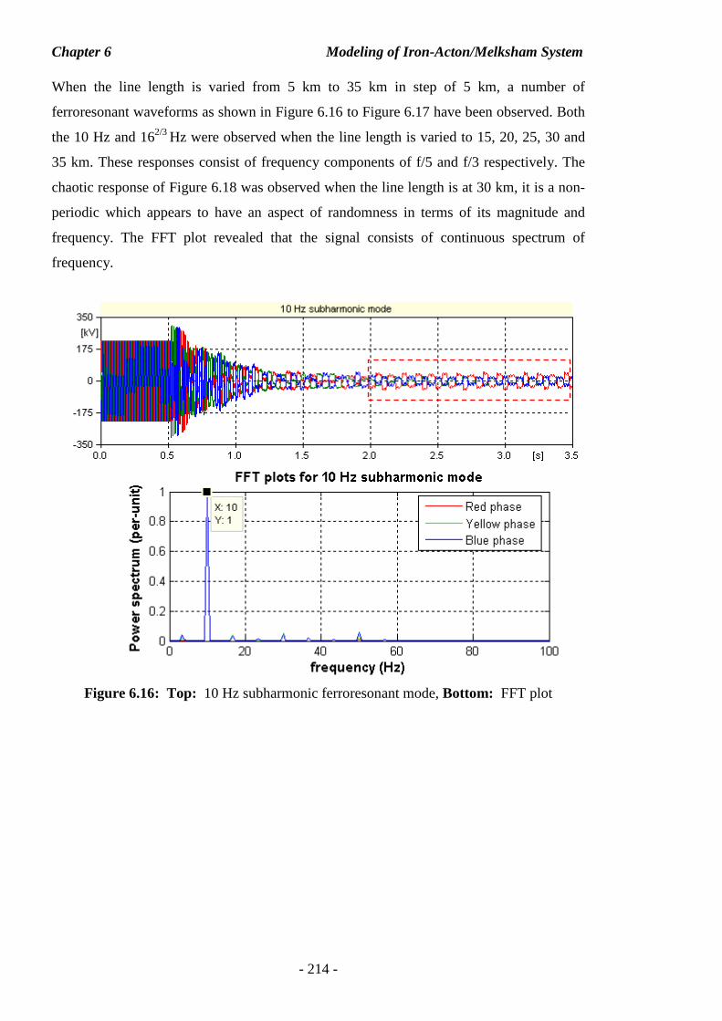
Chapter 6 Modeling of Iron-Acton/Melksham System
- 214 -
When the line length is varied from 5 km to 35 km in step of 5 km, a number of
ferroresonant waveforms as shown in Figure 6.16 to Figure 6.17 have been observed. Both
the 10 Hz and 162/3 Hz were observed when the line length is varied to 15, 20, 25, 30 and
35 km. These responses consist of frequency components of f/5 and f/3 respectively. The
chaotic response of Figure 6.18 was observed when the line length is at 30 km, it is a non-
periodic which appears to have an aspect of randomness in terms of its magnitude and
frequency. The FFT plot revealed that the signal consists of continuous spectrum of
frequency.
Figure 6.16: Top: 10 Hz subharmonic ferroresonant mode, Bottom: FFT plot
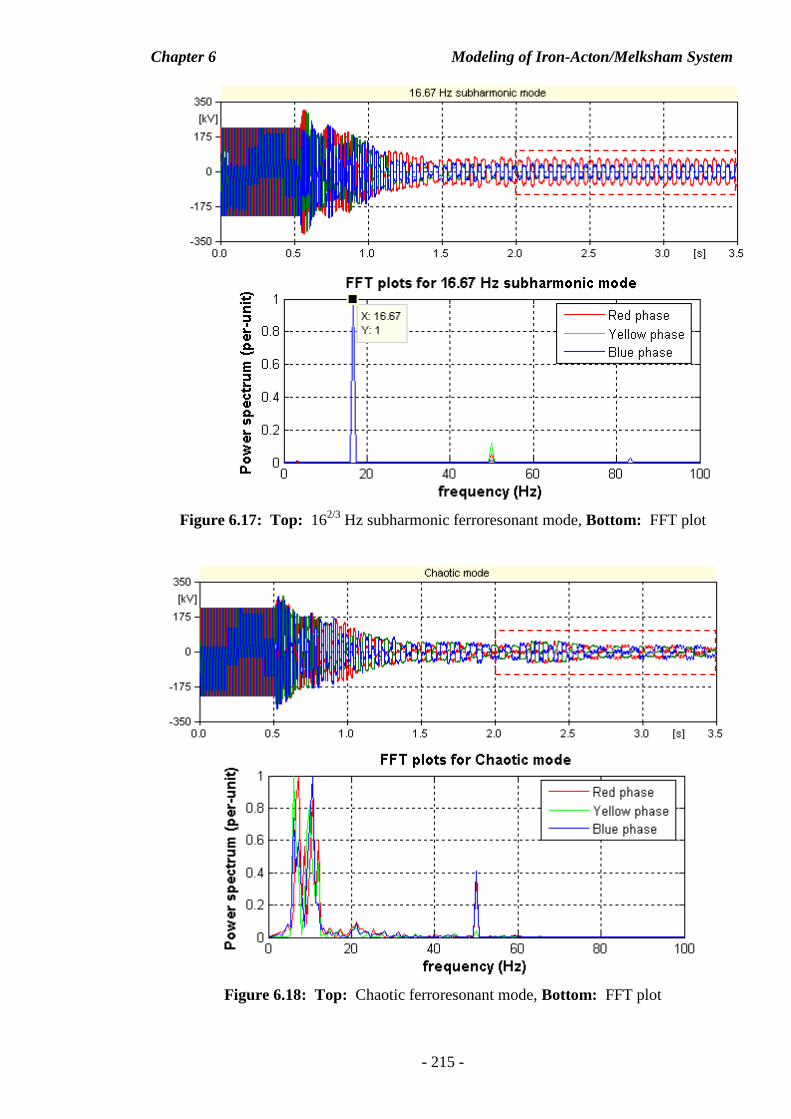
Chapter 6 Modeling of Iron-Acton/Melksham System
- 215 -
Figure 6.17: Top: 162/3 Hz subharmonic ferroresonant mode, Bottom: FFT plot
Figure 6.18: Top: Chaotic ferroresonant mode, Bottom: FFT plot
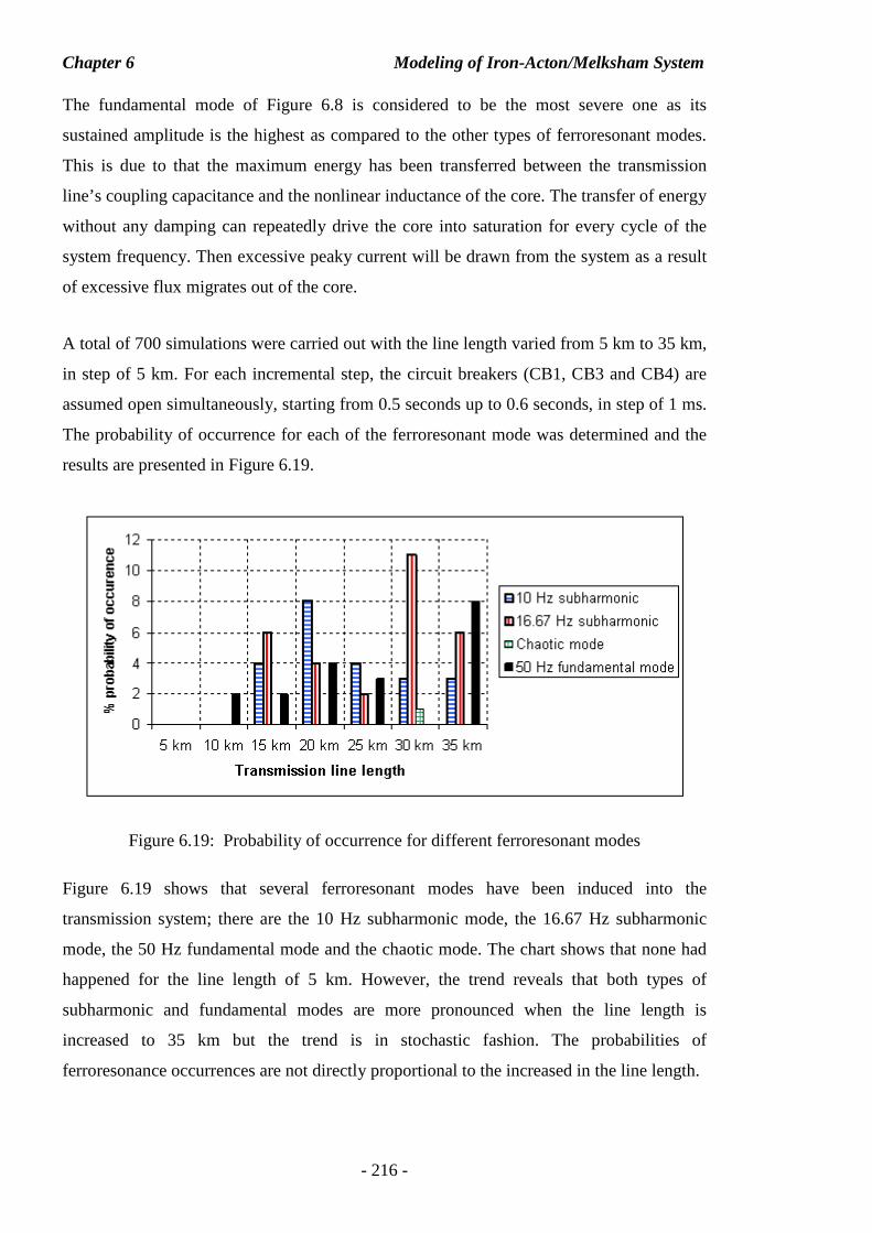
Chapter 6 Modeling of Iron-Acton/Melksham System
- 216 -
The fundamental mode of Figure 6.8 is considered to be the most severe one as its
sustained amplitude is the highest as compared to the other types of ferroresonant modes.
This is due to that the maximum energy has been transferred between the transmission
line’s coupling capacitance and the nonlinear inductance of the core. The transfer of energy
without any damping can repeatedly drive the core into saturation for every cycle of the
system frequency. Then excessive peaky current will be drawn from the system as a result
of excessive flux migrates out of the core.
A total of 700 simulations were carried out with the line length varied from 5 km to 35 km,
in step of 5 km. For each incremental step, the circuit breakers (CB1, CB3 and CB4) are
assumed open simultaneously, starting from 0.5 seconds up to 0.6 seconds, in step of 1 ms.
The probability of occurrence for each of the ferroresonant mode was determined and the
results are presented in Figure 6.19.
Figure 6.19: Probability of occurrence for different ferroresonant modes
Figure 6.19 shows that several ferroresonant modes have been induced into the
transmission system; there are the 10 Hz subharmonic mode, the 16.67 Hz subharmonic
mode, the 50 Hz fundamental mode and the chaotic mode. The chart shows that none had
happened for the line length of 5 km. However, the trend reveals that both types of
subharmonic and fundamental modes are more pronounced when the line length is
increased to 35 km but the trend is in stochastic fashion. The probabilities of
ferroresonance occurrences are not directly proportional to the increased in the line length.
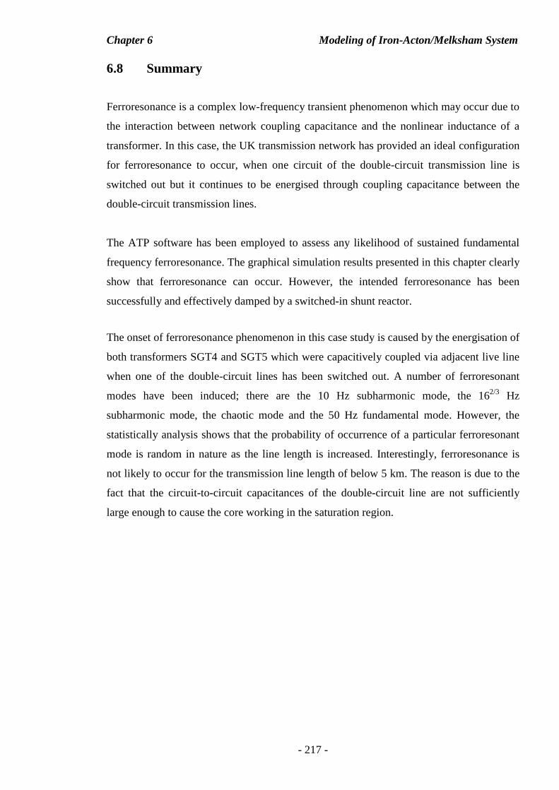
Chapter 6 Modeling of Iron-Acton/Melksham System
- 217 -
6.8 Summary
Ferroresonance is a complex low-frequency transient phenomenon which may occur due to
the interaction between network coupling capacitance and the nonlinear inductance of a
transformer. In this case, the UK transmission network has provided an ideal configuration
for ferroresonance to occur, when one circuit of the double-circuit transmission line is
switched out but it continues to be energised through coupling capacitance between the
double-circuit transmission lines.
The ATP software has been employed to assess any likelihood of sustained fundamental
frequency ferroresonance. The graphical simulation results presented in this chapter clearly
show that ferroresonance can occur. However, the intended ferroresonance has been
successfully and effectively damped by a switched-in shunt reactor.
The onset of ferroresonance phenomenon in this case study is caused by the energisation of
both transformers SGT4 and SGT5 which were capacitively coupled via adjacent live line
when one of the double-circuit lines has been switched out. A number of ferroresonant
modes have been induced; there are the 10 Hz subharmonic mode, the 162/3 Hz
subharmonic mode, the chaotic mode and the 50 Hz fundamental mode. However, the
statistically analysis shows that the probability of occurrence of a particular ferroresonant
mode is random in nature as the line length is increased. Interestingly, ferroresonance is
not likely to occur for the transmission line length of below 5 km. The reason is due to the
fact that the circuit-to-circuit capacitances of the double-circuit line are not sufficiently
large enough to cause the core working in the saturation region.
Chapter 7 Conclusion
218
CHAPTER 7CHAPTER 7CHAPTER 7CHAPTER 7
777... CCCOOONNNCCCLLL UUUSSSIII OOONNN AAANNNDDD FFFUUUTTTUUURRREEE WWWOOORRRKKK
7.1 Conclusion
The study begins by briefly outlining the main function of power system network and the
status of the network due to the development of technological equipment, population
growth and industrial globalisation. Along with network expansion and integration, serious
concern has been raised on the occurrence of transient related events. The consequences of
such event may be system breakdown and catastrophic failure of power system
components such as arrestors, transformers etc.
One of the transients which are likely to be caused by switching events is a low frequency
transient, for example ferroresonance. Prior to the introduction of such a phenomenon, a
linear resonance in a linear R, L and C circuit is firstly discussed, particularly the
mechanism on how resonance can occur in a linear circuit. Then the differences between
the linear resonance and ferroresonance are identified in terms of the system parameters,
the condition for the occurrence of ferroresonance and the types of responses. Several
ferroresonant modes can be identified and they are namely the fundamental mode,
subharmonic mode, quasi-periodic mode and chaotic mode. In addition, the tools to
identify these modes employing frequency spectrum (FFT), Poincaré map and phase-plane
diagram have been presented. This is followed by looking into the implications of
ferroresonance on a power system network, ranging from the mal-operation of protective
device to insulation breakdown. Two general methods of mitigating ferroresonance have
been discussed to avoid the system being put into stress.
Survey into different approaches on modeling of ferroresonance in terms of practical and
simulation aspects has been carried out. There are five categories of ferroresonance studies
which have been presented in the literatures; the analytical approach, the analog simulation
approach, the real field test approach, the laboratory measurement approach and the digital
computer program approach. The drawback of analytical approach is the complexity of the
mathematical model to represent an over simplified circuit. The analog simulation and the
Chapter 7 Conclusion
219
small scale laboratory approaches on the other hand do not truly represent all the
characteristics of the real power network. In contrary, the real field test being carried out
upon the power network will put the test components under stress and even in a dangerous
position. Despite of the major advantages of computer simulation approach, the major
drawback of employing computer simulation for modeling the power system network is the
lack of definite explanation on modeling requirements in terms of selecting the suitable
predefined models and validating the developed models. The only way to find out the
validities of the developed models is to compare the simulation results with the field
recording waveforms.
Prior to the identification of the individual component model and hence the development
of the simulation model for a real case scenario, one of the main aims of this study is to
look into the influence of system parameters on a single-phase ferroresonant circuit. This
includes (1) the study of the influence of magnetising resistance, Rm (2) the study of
influence of degree of core saturations with each case in relation to the change of grading
capacitor of circuit breaker and the ground capacitance. The studies from part (1) turned
out to be that high core-loss has an ability to suppress the sustained Period-1
ferroresonance as compared to low-loss iron core which is employed in modern
transformers. On the other hand, the study from part (2) revealed the followings: (a) high
degree of core saturation – sustained fundamental mode is more likely to occur, however,
subharmonic mode is more likely to happen at high value of shunt capacitor and low value
of grading capacitor (b) low degree of core saturation - fundamental mode occurs at high
value of grading capacitor but limited at higher range of shunt capacitor, however,
subharmonic mode is more likely to occur at high value of shunt capacitor and low value
of grading capacitor. Chaotic mode starts to occur with low degree of core saturation.
The fundamental understanding upon the influence of system parameters on ferroresonance
in a single-phase circuit has been described. Prior to the development of the simulation
model for the real case three-phase power system network, the identification of the models
of the circuit breakers, the transformers and the transmission lines in ATPDraw which are
suitable for ferroresonance study is firstly carried out. The appropriateness of each of the
predefined model is assessed by applying the criteria supported by CIGRE WG 3.02. In
regards to the circuit breaker, a simplistic model based on current zero interruption has
been found to be appropriate as the current study of ferroresonance is only focused on the
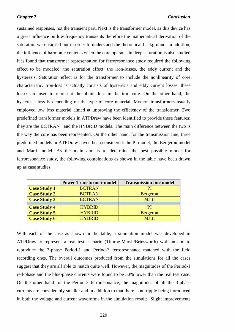
Chapter 7 Conclusion
220
sustained responses, not the transient part. Next is the transformer model, as this device has
a great influence on low frequency transients therefore the mathematical derivation of the
saturation were carried out in order to understand the theoretical background. In addition,
the influence of harmonic contents when the core operates in deep saturation is also studied.
It is found that transformer representation for ferroresonance study required the following
effect to be modeled: the saturation effect, the iron-losses, the eddy current and the
hysteresis. Saturation effect is for the transformer to include the nonlinearity of core
characteristic. Iron-loss is actually consists of hysteresis and eddy current losses, these
losses are used to represent the ohmic loss in the iron core. On the other hand, the
hysteresis loss is depending on the type of core material. Modern transformers usually
employed low loss material aimed at improving the efficiency of the transformer. Two
predefined transformer models in ATPDraw have been identified to provide these features:
they are the BCTRAN+ and the HYBRID models. The main difference between the two is
the way the core has been represented. On the other hand, for the transmission line, three
predefined models in ATPDraw haven been considered: the PI model, the Bergeron model
and Marti model. As the main aim is to determine the best possible model for
ferroresonance study, the following combinations as shown in the table have been drawn
up as case studies.
Power Transformer model Transmission line model Case Study 1 BCTRAN PI Case Study 2 BCTRAN Bergeron Case Study 3 BCTRAN Marti
Case Study 4 HYBRID PI Case Study 5 HYBRID Bergeron Case Study 6 HYBRID Marti
With each of the case as shown in the table, a simulation model was developed in
ATPDraw to represent a real test scenario (Thorpe-Marsh/Brinsworth) with an aim to
reproduce the 3-phase Period-1 and Period-3 ferroresonance matched with the field
recording ones. The overall outcomes produced from the simulations for all the cases
suggest that they are all able to match quite well. However, the magnitudes of the Period-1
red-phase and the blue-phase currents were found to be 50% lower than the real test case.
On the other hand for the Period-3 ferroresonance, the magnitudes of all the 3-phase
currents are considerably smaller and in addition to that there is no ripple being introduced
in both the voltage and current waveforms in the simulation results. Slight improvements
Chapter 7 Conclusion
221
have been made to the simulation model, and the results suggest that only the Period-3
ferroresonance has a slight improvement in terms of their current magnitude and the ripple.
From the study, it is suggested that transmission line using PI model and transformer
employed HYBRID model are the most suitable for ferroresonance study. The
investigations into the key parameter that influence the occurrence of ferroresonance have
been carried out. The study began by looking into the removal of the transformer coupling
capacitance, and then followed by removing cable capacitance, the simulation results
revealed that Period-1 ferroresonance still occurred. Further study is then carried out by
representing the line in lumped parameter in PI representation and each of the coupling
capacitances are then evaluated. The studies showed that the sustainable resonance is
supported by the interaction between the series capacitance (i.e. the circuit-to-circuit
capacitance) and the saturable core inductance. They in fact provide the resonance
condition of matching the saturable core inductive reactances thus providing sustainable
energy transfer. On the other hand, both the ground and line-to-line capacitors supply
additional discharging currents to the core.
Once the types of transmission line and the transformer model have been identified which
are suitable for ferroresonance study, they are then employed to develop another case study
on a National Grid transmission network with an aim to evaluate the likelihood of
occurrence of Period-1 ferroresonance. From the simulation, it has been found that the
Period-1 ferroresonance can be induced into the system. An effort was then carried out to
suppress the phenomena by switching-in the shunt reactor which is connected at the 13 kV
winding side. A series of different shunt reactor ratings have been evaluated and it was
found that a 60 MVAR reactor is able to quench the phenomena in an effective way. In
addition, sensitivity study on transmission line length was also carried out and the
simulation results suggests that sustained fundamental frequency ferroresonance will occur
for the line length of 15, 20, 25, 30 and 35 km.
7.2 Future Work
The major achievement in this project is the identification of the circuit breaker,
transformer and transmission line models which can be used for ferroresonance study.
A simplistic time-controlled switch to represent a circuit breaker can be employed without
considering the circuit breaker’s complex interruption characteristic if a sustained steady-
Chapter 7 Conclusion
222
state phenomenon is of interest. The predefined transformer models namely the BCTRAN+
and the HYBRID are equally capable of representing their saturation effect for the
transformer magnetic core characteristic to account for ferroresonance events. The
transmission line models employing both the lumped-parameter (i.e. the PI representation)
and the distributed-parameter (i.e. the Bergeron and the Marti) models are able to represent
the double-circuit line.
However the predefined models may not be sufficiently accurate when they are used to
represent the power system components, especially when differences are noticed as we
compare the simulation results with the field test recordings. Further work can be done at
the following aspects:
I) The method for modeling the core of the transformer in the predefined model is
based on the open-circuit test report using the 90%, 100% and 110% data. This type of
core representation to account for saturation effect does not characterise the joint effect of
the core when being driven into deep saturation. In fact, transformer driven into deep
saturation may cause more flux distributed into air-gap which in effect will create different
type of core characteristic which is different from the one extrapolated from the open-
circuit test result. Future work on self built transformer core models should be conducted
based on real saturation test results. In the case that the deep saturation test results are not
available, sensitivity studies should be done on the characteristics of the core with various
degrees of deep saturation.
II) For the transmission line model, either the PI, the Bergeron or the Marti models
represents the reactance part of the line well, however the resistive losses are differently
represented and their representation accuracy is hard to assess. For example, there is no
loss in the PI representation, and some spurious oscillation can be seen in the transient
simulation results. In view of this, future work should be focusing on how to accurately
represent the resistive loss in the system and how the loss could affect the initiation of the
ferroresonance phenomena.
III) For the modeling of circuit breaker, the time-controlled switch may be suitable
for the sustained steady-state ferroresonance, however, the detailed interruption
characteristics such as the high frequency transient currents, the time lags of pole

Chapter 7 Conclusion
223
operations and etc may not be fully represented at this stage and can be vital important for
the detail studies of ferroresonance. Such detailed modeling of normal operations of circuit
breakers may require further studies.
Besides, the investigation of the initiation of different modes of ferroresonance is an area
for the future work. The study can be to look into the stochastic manner of the
ferroresonant circuit following the opening of the circuit breaker at different initial
conditions, and to look into the onset conditions of different modes which are sensitive to
system parameters.
References
224
REFERENCESREFERENCESREFERENCESREFERENCES
[1] A. Greenwood, Electrical Transents in Power Systems, Second Edition ed.: John
Willey & Sons, Inc, 1991. [2] J. A. Martinez-Velasco, "Computer Analysis of Electric Power System Transients,"
The Institute of Electrical and Electronics Engineers, Inc, p. 121, 1997. [3] Cadick Corporation, “Ferroresonance” TECHNICAL BULLETIN-004a, May 29,
2002. [4] P. Ferracci, “Ferroresonance, Cashier Technique no 190”, Groupe Schneider. March
1998. [5] C. Charalambous, Z. D. Wang, M. Osborne, and P. Jarman, "Sensitivity studies on
power transformer ferroresonance of a 400 kV double circuit," Generation, Transmission & Distribution, IET, vol. 2, pp. 159-166, 2008.
[6] S. K. Chakravarthy and C. V. Nayar, "Series ferroresonance in power systems," International Journal of Electrical Power & Energy Systems, vol. 17, pp. 267-274, 1995.
[7] C. B. K.Pattanapakdee, "Failure of Riser Pole Arrester due to Station Service Transformer Ferroresonance," in Internatioinal Conference on Power Systems Transients (IPST'07) Lyon, France, 2007.
[8] S. C. Preecha Sakarung, "Application of PSCAD/EMTDC and Chaos Theory to Power System Ferroresonance Analysis," in International Conference on Power Systems Transients (IPST'05) Montreal, Canada, 2005.
[9] Y. Yuhong and Z. Hao, "Study on Simulation of Ferroresonance Elimination in 10kV Power System," in Transmission and Distribution Conference and Exhibition: Asia and Pacific, 2005 IEEE/PES, 2005, pp. 1-7.
[10] B. A. T. Al Zahawi, Z. Emin, and Y. K. Tong, "Chaos in ferroresonant wound voltage transformers: effect of core losses and universal circuit behaviour," Science, Measurement and Technology, IEE Proceedings -, vol. 145, pp. 39-43, 1998.
[11] Z. Emin, B. A. T. Al Zahawi, D. W. Auckland, and Y. K. Tong, "Ferroresonance in electromagnetic voltage transformers: a study based on nonlinear dynamics," Generation, Transmission and Distribution, IEE Proceedings-, vol. 144, pp. 383-387, 1997.
[12] K. Milicevic and Z. Emin, "Impact of initial conditions on the initiation of ferroresonance," International Journal of Electrical Power & Energy Systems, vol. 31, pp. 146-152, 2009.
[13] M. Val Escudero, I. Dudurych, and M. Redfem, "Understanding ferroresonance," in Universities Power Engineering Conference, 2004. UPEC 2004. 39th International, 2004, pp. 1262-1266 vol. 2.
[14] M. Val Escudero, I. Dudurych, and M. A. Redfern, "Characterization of ferroresonant modes in HV substation with CB grading capacitors," Electric Power Systems Research, vol. 77, pp. 1506-1513, 2007.
[15] E. J. Dolan, D. A. Gillies, and E. W. Kimbark, "Ferroresonance in a Transformer Switched with an EHV Line," IEEE Transactions on Power Apparatus and Systems, vol. PAS-91, pp. 1273-1280, 1972.
[16] D. A. N. Jacobson, D. R. Swatek, and R. W. Mazur, "Mitigating potential transformer ferroresonance in a 230 kV converter station," in Transmission and Distribution Conference, 1996. Proceedings., 1996 IEEE, 1996, pp. 269-275.
References
225
[17] J. B. Wareing and F. Perrot, "Ferroresonance overvoltages in distribution networks," in Warning! Ferroresonance Can Damage Your Plant (Digest No: 1997/349), IEE Colloquium on, 1997, pp. 5/1-5/7.
[18] M. Osborne, P. Jarman, C. Charalambous, and Z. D. Wang, "The Impact of Ferroresonance and Low frequency Phenomena on Power Transformers and Transmission Systems," CIGRE, 2007.
[19] J. P. Bickford, Computation of Power System Transients, IEE Monograph Series 18, 1976.
[20] J. A. Martinez, J. Mahseredjian, and R. A. Walling, "Parameter determination: procedures for modeling system transients," Power and Energy Magazine, IEEE, vol. 3, pp. 16-28, 2005.
[21] Z. Emin, B. A. T. Al Zahawi, and Y. K. Tong, "Voltage transformer ferroresonance in 275 kV substation," in High Voltage Engineering, 1999. Eleventh International Symposium on (Conf. Publ. No. 467), 1999, pp. 283-286 vol.1.
[22] Z. Emin, B. A. T. Al Zahawi, T. Yu Kwong, and M. Ugur, "Quantification of the chaotic behavior of ferroresonant voltage transformer circuits," Circuits and Systems I: Fundamental Theory and Applications, IEEE Transactions on, vol. 48, pp. 757-760, 2001.
[23] S. Mozaffari, S. Henschel, and A. C. Soudack, "Chaotic Feroresonance in Power Transformers," IEE Proceeding Generation, Transmission and Distribution, vol. 142, pp. 247-250, May 1995.
[24] Ta-Peng Tsao and Chia-Ching Ning, "Analysis of Ferroresonance Overvoltages at Maanshan Nuclear Power Station in Taiwan," IEEE Transactions on Power Delivery, vol. 21, pp. 1006-1012, April 2006.
[25] S. Mozaffari, M. Sameti, and A. C. Soudack, "Effect of Initial Conditions on Chaotic Ferroresonance in Power Transformers," IEE Proceeding Generation, Transmission and Distribution, vol. 144, pp. 456 - 460, September 1997.
[26] R. F. Karlicek and E. R. Taylor JR., "Ferroresonance of Grounded Potential Transformers on Ungrounded Power Systems," AIEE Transactions, pp. 607-618, August 1959.
[27] R. H. Hopkinson, "Ferroresonance During Single-Phase Switching of 3-Phase Distribution Transformer Banks," power apparatus and systems, ieee transactions on, vol. 84, pp. 289-293, 1965.
[28] R. H. Hopkinson, "Ferroresonant Overvoltage Control Based on TNA Tests on Three-Phase Wye-Delta Transformer Banks," power apparatus and systems, ieee transactions on, vol. PAS-87, pp. 352-361, 1968.
[29] "Ferroresonance Tests on Brinsworth-Thorpe Marsh 400 kV Circuit," Technical Report TR(E) 389 Issue 1, July 2001.
[30] F. S. Young, R. L. Schmid, and P. I. Fergestad, "A Laboratory Investigation of Ferroresonance in Cable-Connected Transformers," power apparatus and systems, ieee transactions on, vol. PAS-87, pp. 1240-1249, 1968.
[31] M. Roy and C. K. Roy, "Experiments on Ferroresonance at Various Line Conditions and Its Damping," in Power System Technology and IEEE Power India Conference, 2008. POWERCON 2008. Joint International Conference on, 2008, pp. 1-8.
[32] T. Fugel and D. Koeing, "Influence of Grading Capacitors on Breaking Performance of a 24-kV Vacuum Breaker Series Design," IEEE Transactions on Dielectrics and Electrical Insulation, vol. 10, pp. 569-575, August 2003.
[33] T. Tran-Quoc and L. Pierrat, "An efficient non linear transformer model and its application to ferroresonance study," Magnetics, IEEE Transactions on, vol. 31, pp. 2060-2063, 1995.
[34] T. Tran-Quoc and L. Pierrat, "Correction of the measured Core Losses under Distorted Flux," IEEE Transactions on Magnetics, vol. 33, pp. 2045-2048, March 1997.
References
226
[35] T. T. Quoc, S. L. Du, D. P. Van, N. N. Khac, and L. T. Dinh, "Temporary overvoltages in the Vietnam 500 kV transmission line," in Transmission & Distribution Construction, Operation & Live-Line Maintenance Proceedings, 1998. ESMO '98. 1998 IEEE 8th International Conference on, 1998, pp. 225-230.
[36] J. R. Marti and A. C. Soudack, "Ferroresonance in power systems: fundamental solutions," Generation, Transmission and Distribution [see also IEE Proceedings-Generation, Transmission and Distribution], IEE Proceedings C, vol. 138, pp. 321-329, 1991.
[37] C. C. Ning and T. P. Tsao, "Using lattice approach to scan nonlinear resonance region," in Transmission and Distribution Conference and Exposition, 2003 IEEE PES, 2003, pp. 13-18 Vol.1.
[38] M. Roy and C. K. Roy, "A study on ferroresonance and its depedence on instant of switching angle of the source voltage," in Power Systems, 2009. ICPS '09. International Conference on, 2009, pp. 1-6.
[39] J. Horak, "A review of ferroresonance," in Protective Relay Engineers, 2004 57th Annual Conference for, 2004, pp. 1-29.
[40] P. Shein, S. Zissu, and W. Schapiro, "Voltage Transformer Ferroresonance in One 400 Kv Gis Substation," in Electrical and Electronics Engineers in Israel, 1989. The Sixteenth Conference of, 1989, pp. 1-5.
[41] A. Belan, Z. Eleschova, and M. Smola, "Resonance overvoltages in electric power networks," in Power Tech, 2005 IEEE Russia, 2005, pp. 1-4.
[42] S. Rahimi, W. Wiechowski, J. Ostergaard, and A. H. Nielsen, "Identification of problems when using long high voltage AC cable in transmission system II: Resonance & harmonic resonance," in Transmission and Distribution Conference and Exposition, 2008. T&D. IEEE/PES, 2008, pp. 1-8.
[43] R. Rudenberg, Transient Performance of Electric Power Systems: McGraw-Hill Book Company, Inc, 1950.
[44] ATP Rule Book and Theory Book, European EMTP-ATP Users Group e.V. (EEUG), 2007.
[45] J. A. Martinez, J. Mahseredjian, and B. Khodabakhchian, "Parameter determination for modeling system transients-Part VI: Circuit breakers," Power Delivery, IEEE Transactions on, vol. 20, pp. 2079-2085, 2005.
[46] J. A. Martinez-Velasco, "Digital Computation of Electromagnetic Transients in Power Systems. Current Status," in EEUG News Feb-May, 1998, pp. 48-70.
[47] "National Grid, UK data sheet, TGN(E)166," February 2002. [48] T. Tran-Quoc, L. Pierrat, A. Montmeat, and A. Giard, "Harmonic overvoltages in
industrial power system with capacitors and saturated transformers," in Industry Applications Conference, 1995. Thirtieth IAS Annual Meeting, IAS '95., Conference Record of the 1995 IEEE, 1995, pp. 2206-2210 vol.3.
[49] T. Tran-Quoc and L. Pierrat, "Influence of Random Variables on Protective Current Transformer Transient Performance," in First International Conference on Digital Power System Simulators (ICDS 95') College Station, Texas, USA, April 5-7,1995.
[50] Bromwich, "Bromwich Formula," http://mathworld.wolfram.com/Multiple-AngleFormulas.html, 1991.
[51] J. A. Martinez, R. Walling, B. A. Mork, J. Martin-Arnedo, and D. Durbak, "Parameter determination for modeling system transients-Part III: Transformers," Power Delivery, IEEE Transactions on, vol. 20, pp. 2051-2062, 2005.
[52] J. A. Martinez and B. A. Mork, "Transformer modeling for low- and mid-frequency transients - a review," Power Delivery, IEEE Transactions on, vol. 20, pp. 1625-1632, 2005.
[53] Juan A. Martinez and B. A. Mork, "Transformer Modeling for Low Frequency Transients - The State of the Art," in International Conference on Power System Transients (IPST 2003) New Orleans, USA, 2003.
References
227
[54] J. A. Martinez-Velasco, "ATP Modeling of Power Transformers," Technical Notes - EEUG News, pp. 63 - 76, Aug - Nov 1998.
[55] V. Brandwajn, H. W. Donnel, and I. I. Dommel, "Matrix Representation of Three-Phase N-Winding Transformers for Steady-State and Transient Studies," Power Apparatus and Systems, IEEE Transactions on, vol. PAS-101, pp. 1369-1378, 1982.
[56] H. K. Hoidalen, "New Features in ATPDraw ver. 4.0 for advanced simulation of electromagnetic transients in power systems," October 2004, pp. 1-58.
[57] B. A. Mork, F. Gonzalez, D. Ishchenko, D. L. Stuehm, and J. Mitra, "Hybrid Transformer Model for Transient Simulation - Part I: Development and Parmeters," IEEE Trans. Power Deliv., pp. 248-255, 2007.
[58] E. Collin Cherry, "The Duality between Interlinked Electric and Magnetic Circuits and the Formation of Transformer Equivalent Circuits," Proceedings of the Physical Society, Part B, vol. 62, pp. 101-111, 1949.
[59] Sung Don Cho, "Parameter Estimation for Transformer Modeling." vol. Ph.D Thesis: Michigan Technological University, USA, 2002.
[60] Hans K. Hoidalen, Bruce A. Mork, Laszlo Prinkler, and James L. Hall, "Implementation of New Features in ATPDraw Version 3," in International Conference on Power Systems Transients - IPST 2003 New Orleans, USA, 2003.
[61] A. I. Ibrahim, S. Henschel, A. C. Lima, and H. W. Dommel, "Applications of a new EMTP line model for short overhead lines and cables," International Journal of Electrical Power & Energy Systems, vol. 24, pp. 639-645, 2002.
[62] Tutorial on Electromagnetic Transient Program Applications to Power System Protection, IEEE Power Engineering Society (PES), 2000.
[63] D. W. Durbak, A. M. Gole, E. H. Camm, M. Marz, R. C. Degeneff, R. P. O'Leary, R. Natarajan, J. A. Martinez-Velasco, K.-C. Lee, A. Morched, R. Shanahan, E. R. Pratico, G. C. Thomann, B. Shperling, A. J. F. Keri, D. A. Woodford, L. Rugeles, V. Rashkes, and A. Sarshar, "Modeling Guidelines for Switching Transients " Report prepared by Switching Tranient Task Force of IEEE Modeling and Analysis of System Transients Working Group 15.08.
[64] A. I. Ibrahim, "An Intelligent Support System For The Analysis of Power System Transients." vol. Ph.D Thesis: University of British Columbia, 2000.
[65] J. R. Marti, "Accurate Modeling of Frequency Dependent Transmission Lines in Electromagnetic Transient Simulations," IEEE Transactions on Power Apparatus and Systems, vol. PAS-101, pp. 147 - 157, January 1982.
[66] J. R. Marti, L. Marti, and H. W. Dommel, "Transmission Line Models for Steady-State and Transients Analysis," IEEE/NTUA Athens Power Tech Conference: "Planning Operation and Control of Today's Electric Power Systems" pp. 744 - 750, Sept 5-8, 1993.
[67] Neville Watson and Jos Arrillaga, Power Systems Electromagnetic Transients Simulation, IET Power and Energy Seried 39, 2007.
[68] D. A. N. Jacobson, L. Marti, and R. W. Menzies, "Modeling Ferroresonance in a 230 kV Transformer-Terminated Double-Circuit Transmission Line," IPST'99 International Conference on Power Systems Transients, pp. 451-456, June 20-24, 1999.
[69] M. R. Iravani, A. K. S. Chaudhary, W. J. Giesbrecht, I. E. Hassan, A. J. F. Keri, K. C. Lee, J. A. Martinez, A. S. Morched, B. A. Mork, M. Parniani, A. Sharshar, D. Shirmohammadi, R. A. Walling, and D. A. Woodford, "Modeling and analysis guidelines for slow transients. III. The study of ferroresonance," Power Delivery, IEEE Transactions on, vol. 15, pp. 255-265, 2000.
[70] G. F. Moore, Electric Cable Handbook 3rd Edition ed.: Blackwell Publishing, 1997. [71] "Transformers Test Report - National Grid."

References
228
[72] Y. K. Tong, "NGC experience on ferroresonance in power transformers and voltage transformers on HV transmission systems," IEE Seminar Digests, vol. 1997, pp. 4-4, 1997.
[73] T. D. Burton, Introduction to Dynamic System Analysis, International Edition ed.: McGraw-Hill.
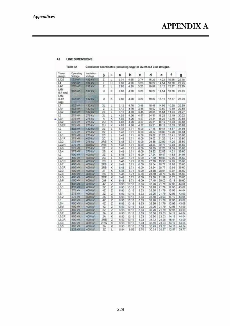
Appendices
229
APPENDIAPPENDIAPPENDIAPPENDIX AX AX AX A
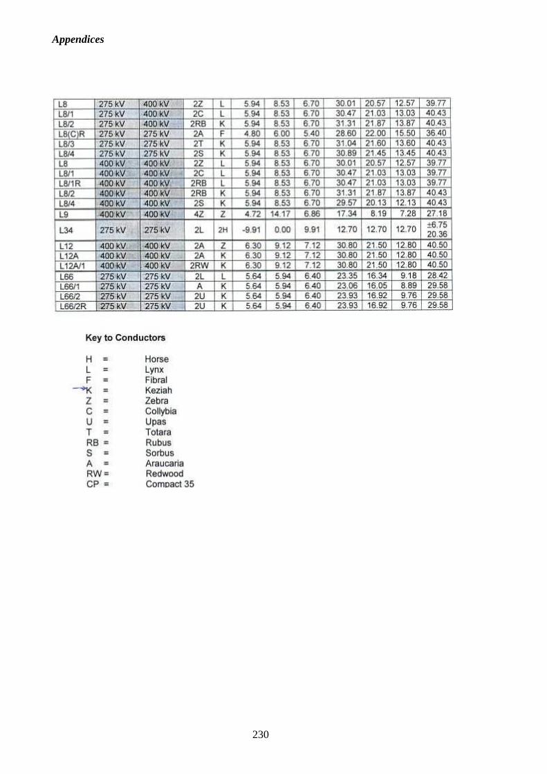
Appendices
230
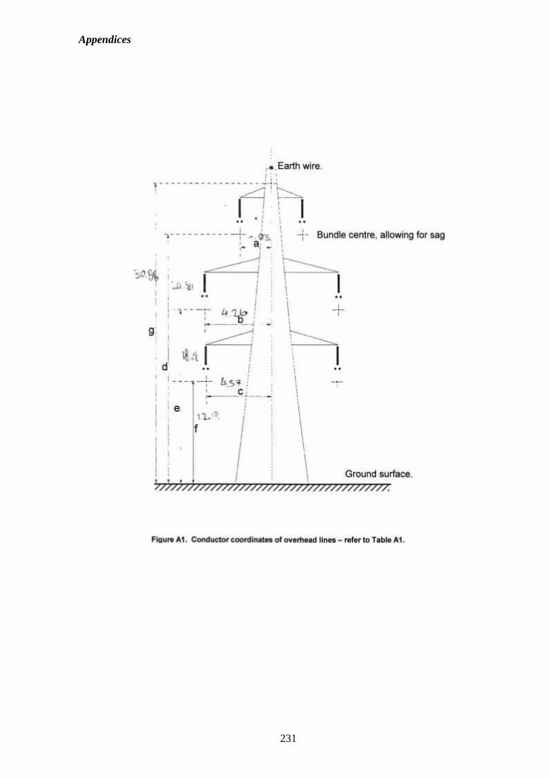
Appendices
231
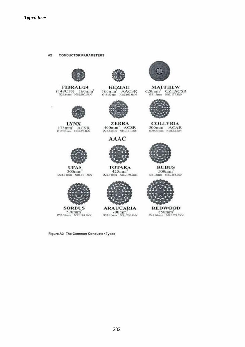
Appendices
232
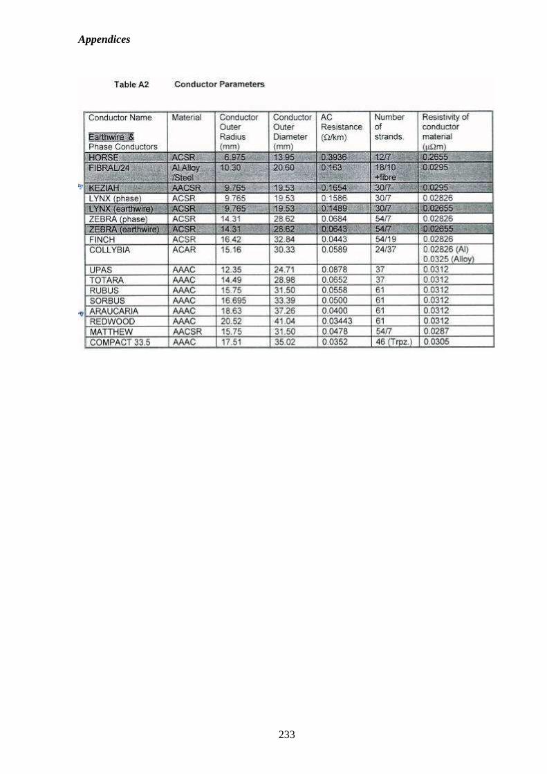
Appendices
233
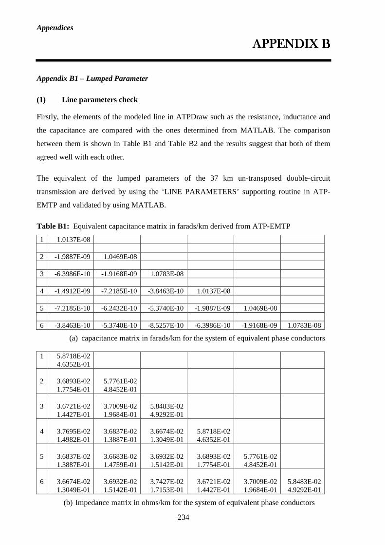
Appendices
234
APPENDIX BAPPENDIX BAPPENDIX BAPPENDIX B
Appendix B1 – Lumped Parameter
(1) Line parameters check
Firstly, the elements of the modeled line in ATPDraw such as the resistance, inductance and
the capacitance are compared with the ones determined from MATLAB. The comparison
between them is shown in Table B1 and Table B2 and the results suggest that both of them
agreed well with each other.
The equivalent of the lumped parameters of the 37 km un-transposed double-circuit
transmission are derived by using the ‘LINE PARAMETERS’ supporting routine in ATP-
EMTP and validated by using MATLAB.
Table B1: Equivalent capacitance matrix in farads/km derived from ATP-EMTP
1 1.0137E-08 2 -1.9887E-09 1.0469E-08 3 -6.3986E-10 -1.9168E-09 1.0783E-08 4 -1.4912E-09 -7.2185E-10 -3.8463E-10 1.0137E-08 5 -7.2185E-10 -6.2432E-10 -5.3740E-10 -1.9887E-09 1.0469E-08 6 -3.8463E-10 -5.3740E-10 -8.5257E-10 -6.3986E-10 -1.9168E-09 1.0783E-08
(a) capacitance matrix in farads/km for the system of equivalent phase conductors 1 5.8718E-02 4.6352E-01
2 3.6893E-02 5.7761E-02 1.7754E-01 4.8452E-01 3 3.6721E-02 3.7009E-02 5.8483E-02 1.4427E-01 1.9684E-01 4.9292E-01 4 3.7695E-02 3.6837E-02 3.6674E-02 5.8718E-02 1.4982E-01 1.3887E-01 1.3049E-01 4.6352E-01 5 3.6837E-02 3.6683E-02 3.6932E-02 3.6893E-02 5.7761E-02 1.3887E-01 1.4759E-01 1.5142E-01 1.7754E-01 4.8452E-01 6 3.6674E-02 3.6932E-02 3.7427E-02 3.6721E-02 3.7009E-02 5.8483E-02 1.3049E-01 1.5142E-01 1.7153E-01 1.4427E-01 1.9684E-01 4.9292E-01
(b) Impedance matrix in ohms/km for the system of equivalent phase conductors
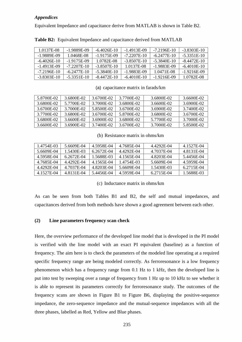
Appendices
235
Equivalent Impedance and capacitance derive from MATLAB is shown in Table B2.
Table B2: Equivalent Impedance and capacitance derived from MATLAB
1.0137E-08 -1.9889E-09 -6.4026E-10 -1.4913E-09 -7.2196E-10 -3.8303E-10 -1.9889E-09 1.0468E-08 -1.9175E-09 -7.2207E-10 -6.2477E-10 -5.3351E-10 -6.4026E-10 -1.9175E-09 1.0782E-08 -3.8507E-10 -5.3840E-10 -8.4472E-10 -1.4913E-09 -7.2207E-10 -3.8507E-10 1.0137E-08 -1.9883E-09 -6.4010E-10 -7.2196E-10 -6.2477E-10 -5.3840E-10 -1.9883E-09 1.0471E-08 -1.9216E-09 -3.8303E-10 -5.3351E-10 -8.4472E-10 -6.4010E-10 -1.9216E-09 1.0782E-08
(a) capacitance matrix in farads/km
5.8700E-02 3.6800E-02 3.6700E-02 3.7700E-02 3.6800E-02 3.6600E-02 3.6800E-02 5.7700E-02 3.7000E-02 3.6800E-02 3.6600E-02 3.6900E-02 3.6700E-02 3.7000E-02 5.8500E-02 3.6700E-02 3.6900E-02 3.7400E-02 3.7700E-02 3.6800E-02 3.6700E-02 5.8700E-02 3.6800E-02 3.6700E-02 3.6800E-02 3.6600E-02 3.6900E-02 3.6800E-02 5.7700E-02 3.7000E-02 3.6600E-02 3.6900E-02 3.7400E-02 3.6700E-02 3.7000E-02 5.8500E-02
(b) Resistance matrix in ohms/km
1.4754E-03 5.6609E-04 4.5958E-04 4.7685E-04 4.4292E-04 4.1527E-04 5.6609E-04 1.5430E-03 6.2672E-04 4.4292E-04 4.7037E-04 4.8131E-04 4.5958E-04 6.2672E-04 1.5688E-03 4.1565E-04 4.8203E-04 5.4456E-04 4.7685E-04 4.4292E-04 4.1565E-04 1.4754E-03 5.6609E-04 4.5959E-04 4.4292E-04 4.7037E-04 4.8203E-04 5.6609E-04 1.5430E-03 6.2715E-04 4.1527E-04 4.8131E-04 5.4456E-04 4.5959E-04 6.2715E-04 1.5688E-03
(c) Inductance matrix in ohms/km
As can be seen from both Tables B1 and B2, the self and mutual impedances, and
capacitances derived from both methods have shown a good agreement between each other.
(2) Line parameters frequency scan check
Here, the overview performance of the developed line model that is developed in the PI model
is verified with the line model with an exact PI equivalent (baseline) as a function of
frequency. The aim here is to check the parameters of the modeled line operating at a required
specific frequency range are being modeled correctly. As ferroresonance is a low frequency
phenomenon which has a frequency range from 0.1 Hz to 1 kHz, then the developed line is
put into test by sweeping over a range of frequency from 1 Hz up to 10 kHz to see whether it
is able to represent its parameters correctly for ferroresonance study. The outcomes of the
frequency scans are shown in Figure B1 to Figure B6, displaying the positive-sequence
impedance, the zero-sequence impedance and the mutual-sequence impedances with all the
three phases, labelled as Red, Yellow and Blue phases.
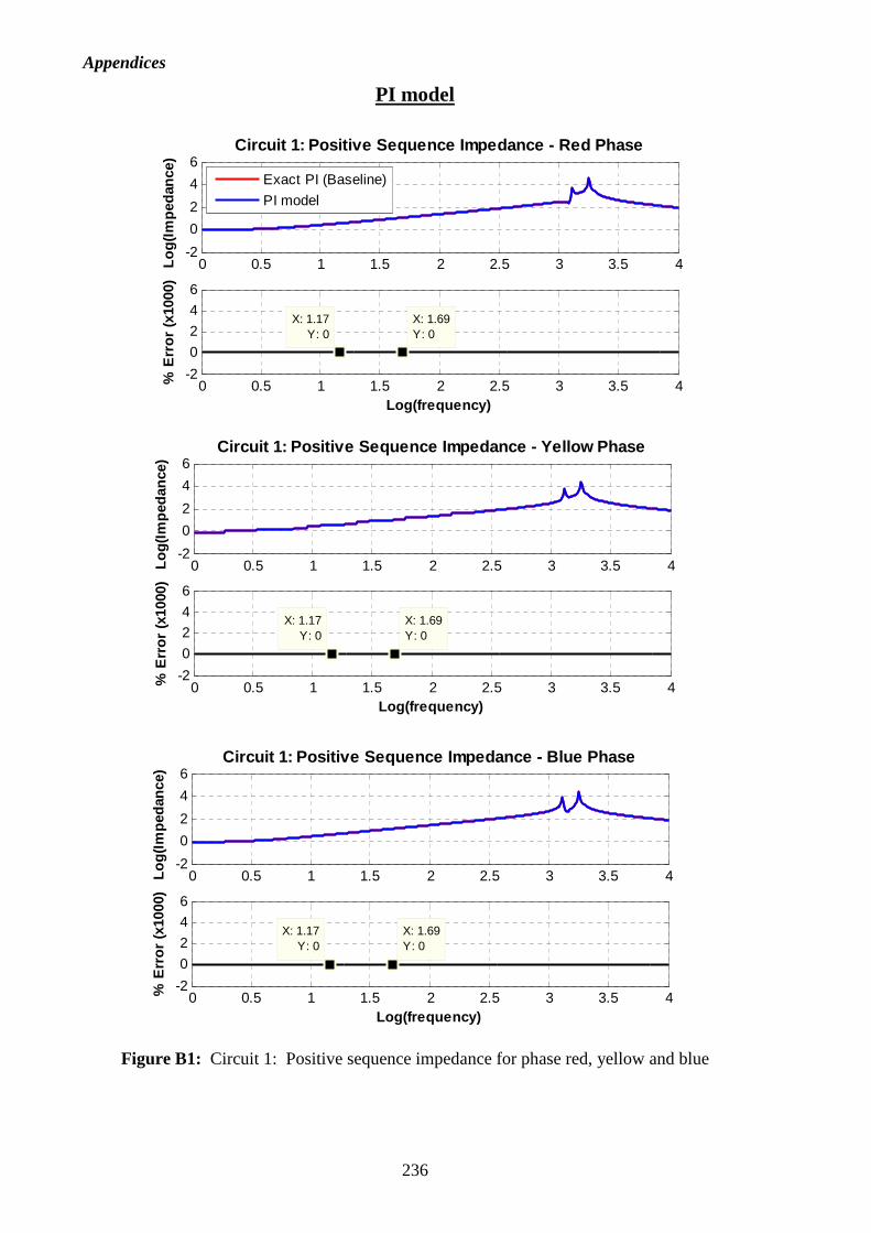
Appendices
236
PI model
Figure B1: Circuit 1: Positive sequence impedance for phase red, yellow and blue
0 0.5 1 1.5 2 2.5 3 3.5 4-2
0
2
4
6
Log(
Impe
danc
e)
Circuit 1: Positive Sequence Impedance - Blue Phase
0 0.5 1 1.5 2 2.5 3 3.5 4-2
0
2
4
6
X: 1.17Y: 0
% E
rror
(x1
000)
Log(frequency)
X: 1.69Y: 0
0 0.5 1 1.5 2 2.5 3 3.5 4-2
0
2
4
6
Log(
Impe
danc
e)
Circuit 1: Positive Sequence Impedance - Yellow Pha se
0 0.5 1 1.5 2 2.5 3 3.5 4-2
0
2
4
6
X: 1.17Y: 0
% E
rror
(x1
000)
Log(frequency)
X: 1.69Y: 0
0 0.5 1 1.5 2 2.5 3 3.5 4-2
0
2
4
6Lo
g(Im
peda
nce)
Circuit 1: Positive Sequence Impedance - Red Phase
0 0.5 1 1.5 2 2.5 3 3.5 4-2
0
2
4
6
X: 1.69Y: 0
% E
rror
(x1
000)
Log(frequency)
X: 1.17Y: 0
Exact PI (Baseline)
PI model
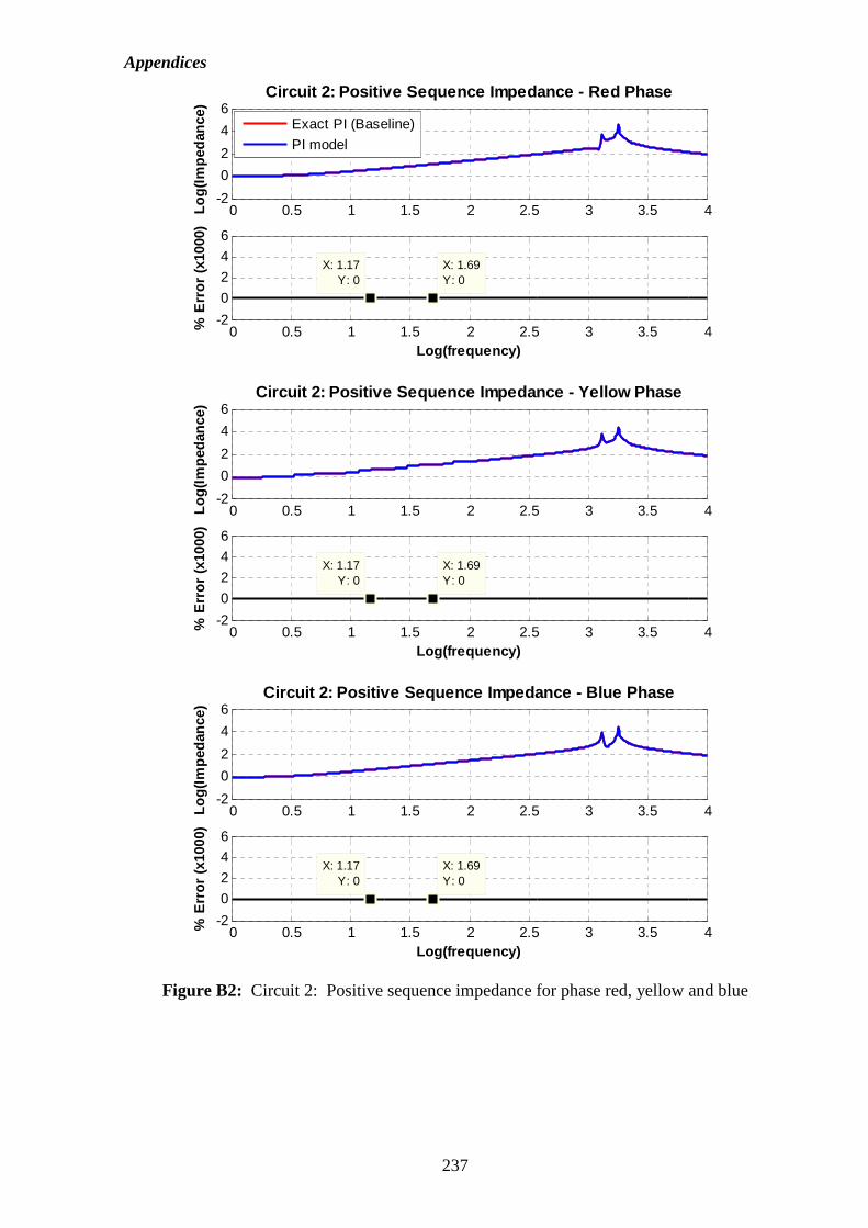
Appendices
237
Figure B2: Circuit 2: Positive sequence impedance for phase red, yellow and blue
0 0.5 1 1.5 2 2.5 3 3.5 4-2
0
2
4
6
Log(
Impe
danc
e)
Circuit 2: Positive Sequence Impedance - Blue Phase
0 0.5 1 1.5 2 2.5 3 3.5 4-2
0
2
4
6
X: 1.17Y: 0
% E
rror
(x1
000)
Log(frequency)
X: 1.69Y: 0
0 0.5 1 1.5 2 2.5 3 3.5 4-2
0
2
4
6
Log(
Impe
danc
e)
Circuit 2: Positive Sequence Impedance - Yellow Pha se
0 0.5 1 1.5 2 2.5 3 3.5 4-2
0
2
4
6
X: 1.17Y: 0
% E
rror
(x1
000)
Log(frequency)
X: 1.69Y: 0
0 0.5 1 1.5 2 2.5 3 3.5 4-2
0
2
4
6
Log(
Impe
danc
e)
Circuit 2: Positive Sequence Impedance - Red Phase
0 0.5 1 1.5 2 2.5 3 3.5 4-2
0
2
4
6
X: 1.17Y: 0
% E
rror
(x1
000)
Log(frequency)
X: 1.69Y: 0
Exact PI (Baseline)
PI model
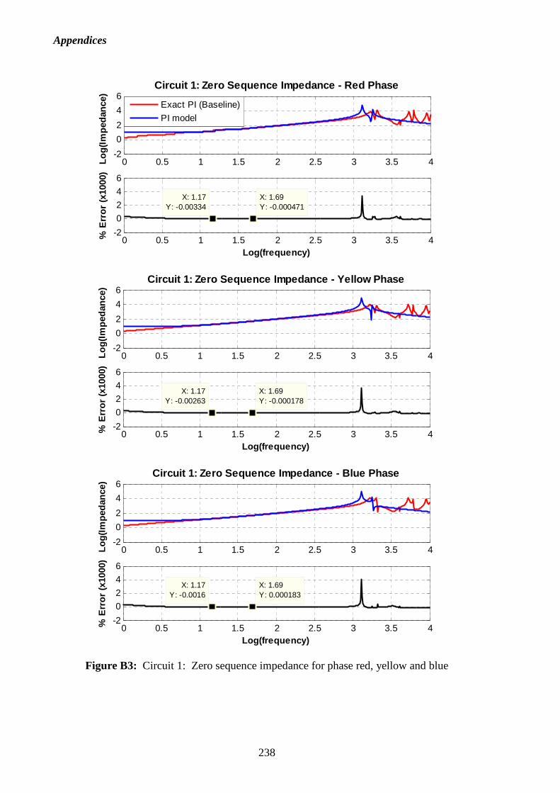
Appendices
238
Figure B3: Circuit 1: Zero sequence impedance for phase red, yellow and blue
0 0.5 1 1.5 2 2.5 3 3.5 4-2
0
2
4
6
Log(
Impe
danc
e)
Circuit 1: Zero Sequence Impedance - Blue Phase
0 0.5 1 1.5 2 2.5 3 3.5 4-2
0
2
4
6
X: 1.17Y: -0.0016
% E
rror
(x1
000)
Log(frequency)
X: 1.69Y: 0.000183
0 0.5 1 1.5 2 2.5 3 3.5 4-2
0
2
4
6
Log(
Impe
danc
e)
Circuit 1: Zero Sequence Impedance - Yellow Phase
0 0.5 1 1.5 2 2.5 3 3.5 4-2
0
2
4
6
X: 1.17Y: -0.00263
% E
rror
(x1
000)
Log(frequency)
X: 1.69Y: -0.000178
0 0.5 1 1.5 2 2.5 3 3.5 4-2
0
2
4
6Lo
g(Im
peda
nce)
Circuit 1: Zero Sequence Impedance - Red Phase
0 0.5 1 1.5 2 2.5 3 3.5 4-2
0
2
4
6
X: 1.17Y: -0.00334
% E
rror
(x1
000)
Log(frequency)
X: 1.69Y: -0.000471
Exact PI (Baseline)
PI model
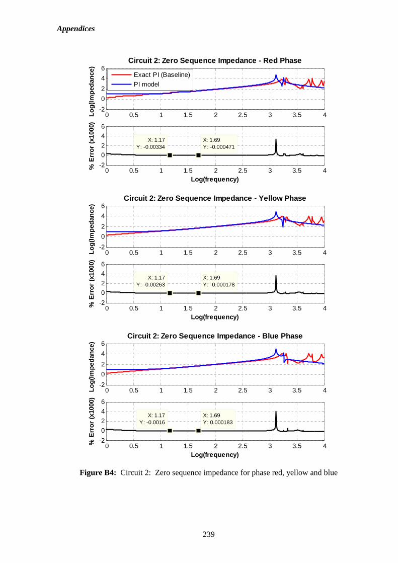
Appendices
239
Figure B4: Circuit 2: Zero sequence impedance for phase red, yellow and blue
0 0.5 1 1.5 2 2.5 3 3.5 4-2
0
2
4
6
Log(
Impe
danc
e)
Circuit 2: Zero Sequence Impedance - Blue Phase
0 0.5 1 1.5 2 2.5 3 3.5 4-2
0
2
4
6
X: 1.17Y: -0.0016
% E
rror
(x1
000)
Log(frequency)
X: 1.69Y: 0.000183
0 0.5 1 1.5 2 2.5 3 3.5 4-2
0
2
4
6
Log(
Impe
danc
e)
Circuit 2: Zero Sequence Impedance - Yellow Phase
0 0.5 1 1.5 2 2.5 3 3.5 4-2
0
2
4
6
X: 1.17Y: -0.00263
% E
rror
(x1
000)
Log(frequency)
X: 1.69Y: -0.000178
0 0.5 1 1.5 2 2.5 3 3.5 4-2
0
2
4
6
Log(
Impe
danc
e)
Circuit 2: Zero Sequence Impedance - Red Phase
0 0.5 1 1.5 2 2.5 3 3.5 4-2
0
2
4
6
X: 1.17Y: -0.00334
% E
rror
(x1
000)
Log(frequency)
X: 1.69Y: -0.000471
Exact PI (Baseline)
PI model
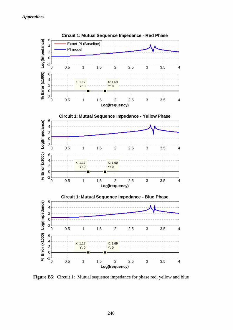
Appendices
240
Figure B5: Circuit 1: Mutual sequence impedance for phase red, yellow and blue
0 0.5 1 1.5 2 2.5 3 3.5 4-2
0
2
4
6
Log(
Impe
danc
e)
Circuit 1: Mutual Sequence Impedance - Blue Phase
0 0.5 1 1.5 2 2.5 3 3.5 4-2
0
2
4
6
X: 1.17Y: 0
% E
rror
(x1
000)
Log(frequency)
X: 1.69Y: 0
0 0.5 1 1.5 2 2.5 3 3.5 4-2
0
2
4
6
Log(
Impe
danc
e)
Circuit 1: Mutual Sequence Impedance - Yellow Phase
0 0.5 1 1.5 2 2.5 3 3.5 4-2
0
2
4
6
X: 1.17Y: 0
% E
rror
(x1
000)
Log(frequency)
X: 1.69Y: 0
0 0.5 1 1.5 2 2.5 3 3.5 4-2
0
2
4
6Lo
g(Im
peda
nce)
Circuit 1: Mutual Sequence Impedance - Red Phase
0 0.5 1 1.5 2 2.5 3 3.5 4-2
0
2
4
6
X: 1.17Y: 0
% E
rror
(x1
000)
Log(frequency)
X: 1.69Y: 0
Exact PI (Baseline)
PI model
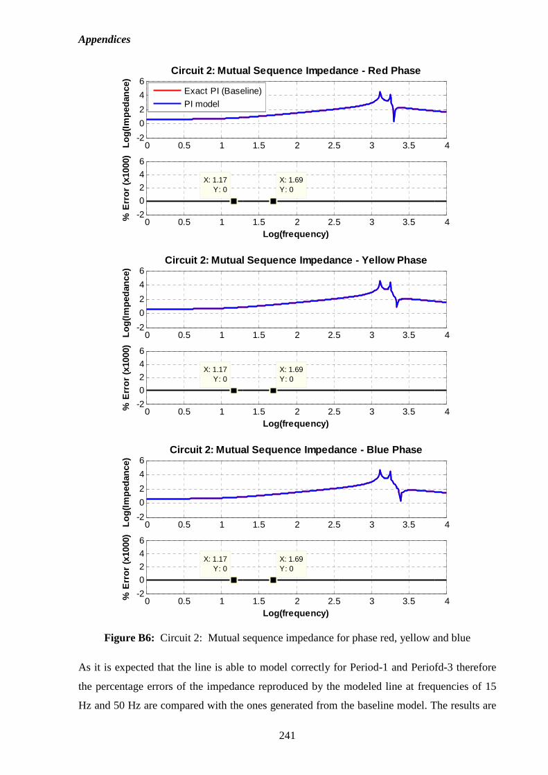
Appendices
241
Figure B6: Circuit 2: Mutual sequence impedance for phase red, yellow and blue
As it is expected that the line is able to model correctly for Period-1 and Periofd-3 therefore
the percentage errors of the impedance reproduced by the modeled line at frequencies of 15
Hz and 50 Hz are compared with the ones generated from the baseline model. The results are
0 0.5 1 1.5 2 2.5 3 3.5 4-2
0
2
4
6
Log(
Impe
danc
e)
Circuit 2: Mutual Sequence Impedance - Blue Phase
0 0.5 1 1.5 2 2.5 3 3.5 4-2
0
2
4
6
X: 1.17Y: 0
% E
rror
(x1
000)
Log(frequency)
X: 1.69Y: 0
0 0.5 1 1.5 2 2.5 3 3.5 4-2
0
2
4
6
Log(
Impe
danc
e)
Circuit 2: Mutual Sequence Impedance - Yellow Phase
0 0.5 1 1.5 2 2.5 3 3.5 4-2
0
2
4
6
X: 1.17Y: 0
% E
rror
(x1
000)
Log(frequency)
X: 1.69Y: 0
0 0.5 1 1.5 2 2.5 3 3.5 4-2
0
2
4
6
Log(
Impe
danc
e)
Circuit 2: Mutual Sequence Impedance - Red Phase
0 0.5 1 1.5 2 2.5 3 3.5 4-2
0
2
4
6
X: 1.17Y: 0
% E
rror
(x1
000)
Log(frequency)
X: 1.69Y: 0
Exact PI (Baseline)
PI model
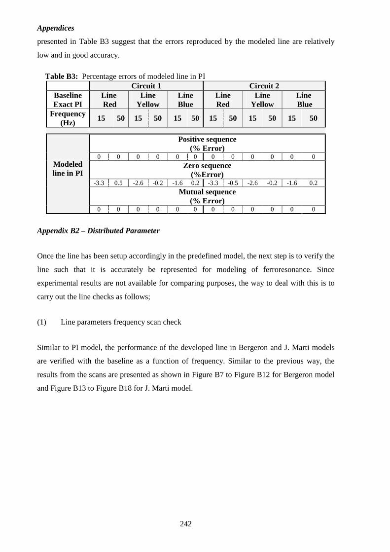
Appendices
242
presented in Table B3 suggest that the errors reproduced by the modeled line are relatively
low and in good accuracy.
Table B3: Percentage errors of modeled line in PI Circuit 1 Circuit 2 Baseline Exact PI
Line Red
Line Yellow
Line Blue
Line Red
Line Yellow
Line Blue
Frequency (Hz)
15 50 15 50 15 50 15 50 15 50 15 50
Positive sequence (% Error)
0 0 0 0 0 0 0 0 0 0 0 0
Zero sequence (%Error)
-3.3 0.5 -2.6 -0.2 -1.6 0.2 -3.3 -0.5 -2.6 -0.2 -1.6 0.2
Mutual sequence (% Error)
Modeled line in PI
0 0 0 0 0 0 0 0 0 0 0 0
Appendix B2 – Distributed Parameter
Once the line has been setup accordingly in the predefined model, the next step is to verify the
line such that it is accurately be represented for modeling of ferroresonance. Since
experimental results are not available for comparing purposes, the way to deal with this is to
carry out the line checks as follows;
(1) Line parameters frequency scan check
Similar to PI model, the performance of the developed line in Bergeron and J. Marti models
are verified with the baseline as a function of frequency. Similar to the previous way, the
results from the scans are presented as shown in Figure B7 to Figure B12 for Bergeron model
and Figure B13 to Figure B18 for J. Marti model.
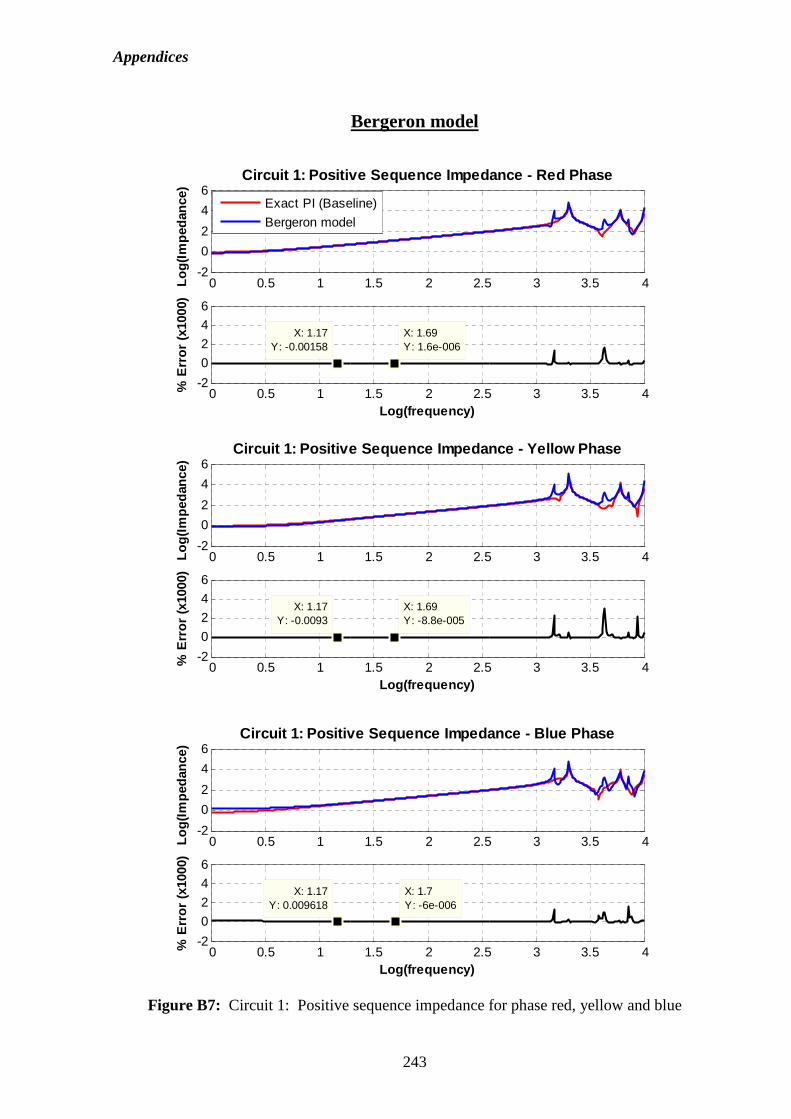
Appendices
243
Bergeron model
Figure B7: Circuit 1: Positive sequence impedance for phase red, yellow and blue
0 0.5 1 1.5 2 2.5 3 3.5 4-2
0
2
4
6
Log(
Impe
danc
e)
Circuit 1: Positive Sequence Impedance - Blue Phase
0 0.5 1 1.5 2 2.5 3 3.5 4-2
0
2
4
6
X: 1.17Y: 0.009618
% E
rror
(x1
000)
Log(frequency)
X: 1.7Y: -6e-006
0 0.5 1 1.5 2 2.5 3 3.5 4-2
0
2
4
6
Log(
Impe
danc
e)
Circuit 1: Positive Sequence Impedance - Yellow Pha se
0 0.5 1 1.5 2 2.5 3 3.5 4-2
0
2
4
6
X: 1.17Y: -0.0093
% E
rror
(x1
000)
Log(frequency)
X: 1.69Y: -8.8e-005
0 0.5 1 1.5 2 2.5 3 3.5 4-2
0
2
4
6Lo
g(Im
peda
nce)
Circuit 1: Positive Sequence Impedance - Red Phase
0 0.5 1 1.5 2 2.5 3 3.5 4-2
0
2
4
6
X: 1.17Y: -0.00158
% E
rror
(x1
000)
Log(frequency)
X: 1.69Y: 1.6e-006
Exact PI (Baseline)
Bergeron model
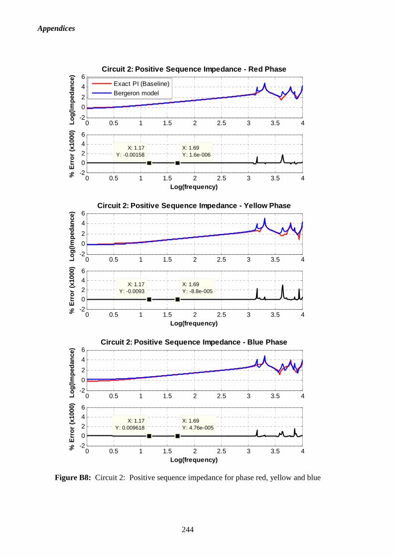
Appendices
244
Figure B8: Circuit 2: Positive sequence impedance for phase red, yellow and blue
0 0.5 1 1.5 2 2.5 3 3.5 4-2
0
2
4
6
Log(
Impe
danc
e)
Circuit 2: Positive Sequence Impedance - Blue Phase
0 0.5 1 1.5 2 2.5 3 3.5 4-2
0
2
4
6
X: 1.17Y: 0.009618
% E
rror
(x1
000)
Log(frequency)
X: 1.69Y: 4.76e-005
0 0.5 1 1.5 2 2.5 3 3.5 4-2
0
2
4
6
Log(
Impe
danc
e)
Circuit 2: Positive Sequence Impedance - Yellow Pha se
0 0.5 1 1.5 2 2.5 3 3.5 4-2
0
2
4
6
X: 1.17Y: -0.0093
% E
rror
(x1
000)
Log(frequency)
X: 1.69Y: -8.8e-005
0 0.5 1 1.5 2 2.5 3 3.5 4-2
0
2
4
6Lo
g(Im
peda
nce)
Circuit 2: Positive Sequence Impedance - Red Phase
0 0.5 1 1.5 2 2.5 3 3.5 4-2
0
2
4
6
X: 1.17Y: -0.00158
% E
rror
(x1
000)
Log(frequency)
X: 1.69Y: 1.6e-006
Exact PI (Baseline)
Bergeron model
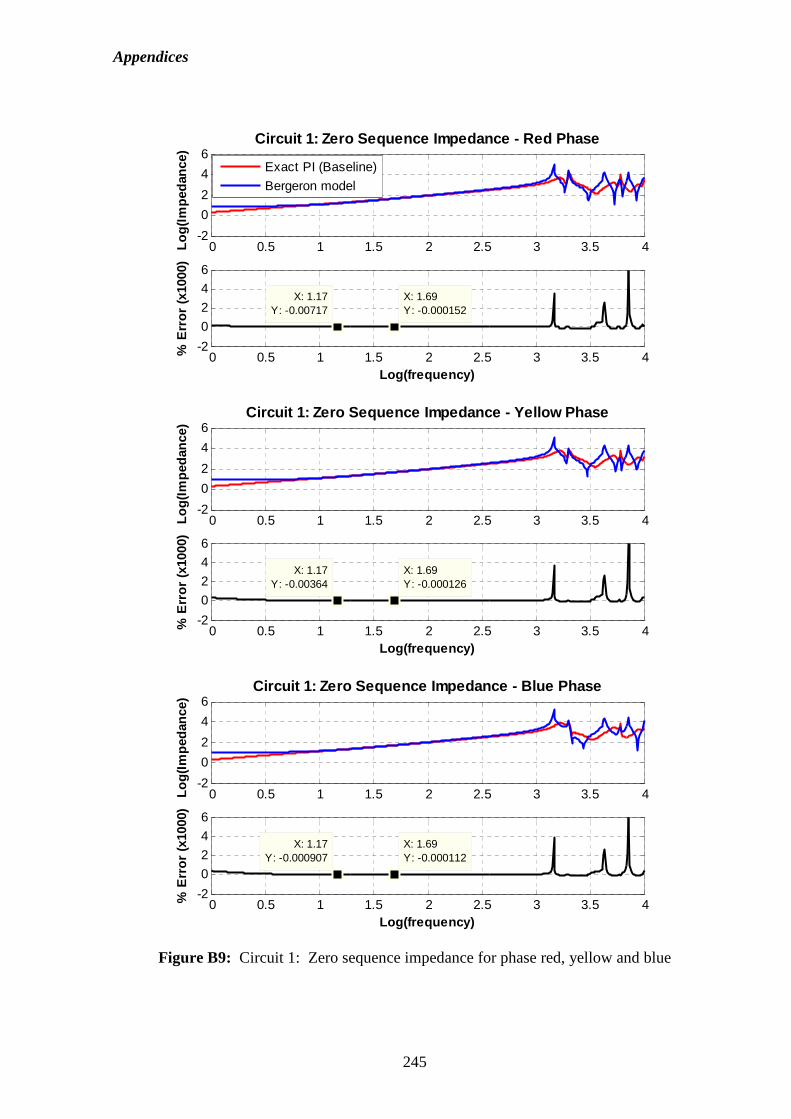
Appendices
245
Figure B9: Circuit 1: Zero sequence impedance for phase red, yellow and blue
0 0.5 1 1.5 2 2.5 3 3.5 4-2
0
2
4
6
Log(
Impe
danc
e)
Circuit 1: Zero Sequence Impedance - Blue Phase
0 0.5 1 1.5 2 2.5 3 3.5 4-2
0
2
4
6
X: 1.17Y: -0.000907
% E
rror
(x1
000)
Log(frequency)
X: 1.69Y: -0.000112
0 0.5 1 1.5 2 2.5 3 3.5 4-2
0
2
4
6
Log(
Impe
danc
e)
Circuit 1: Zero Sequence Impedance - Yellow Phase
0 0.5 1 1.5 2 2.5 3 3.5 4-2
0
2
4
6
X: 1.17Y: -0.00364
% E
rror
(x1
000)
Log(frequency)
X: 1.69Y: -0.000126
0 0.5 1 1.5 2 2.5 3 3.5 4-2
0
2
4
6
Log(
Impe
danc
e)
Circuit 1: Zero Sequence Impedance - Red Phase
0 0.5 1 1.5 2 2.5 3 3.5 4-2
0
2
4
6
X: 1.17Y: -0.00717
% E
rror
(x1
000)
Log(frequency)
X: 1.69Y: -0.000152
Exact PI (Baseline)
Bergeron model
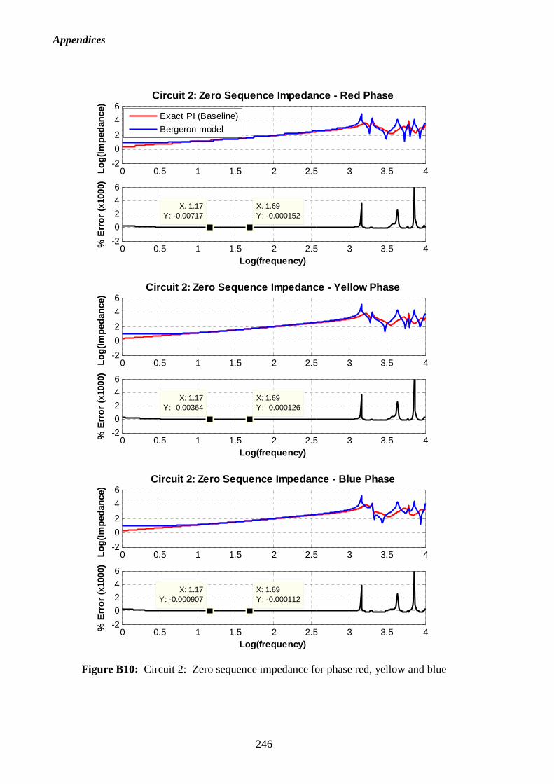
Appendices
246
Figure B10: Circuit 2: Zero sequence impedance for phase red, yellow and blue
0 0.5 1 1.5 2 2.5 3 3.5 4-2
0
2
4
6
Log(
Impe
danc
e)
Circuit 2: Zero Sequence Impedance - Blue Phase
0 0.5 1 1.5 2 2.5 3 3.5 4-2
0
2
4
6
X: 1.17Y: -0.000907
% E
rror
(x1
000)
Log(frequency)
X: 1.69Y: -0.000112
0 0.5 1 1.5 2 2.5 3 3.5 4-2
0
2
4
6
Log(
Impe
danc
e)
Circuit 2: Zero Sequence Impedance - Yellow Phase
0 0.5 1 1.5 2 2.5 3 3.5 4-2
0
2
4
6
X: 1.17Y: -0.00364
% E
rror
(x1
000)
Log(frequency)
X: 1.69Y: -0.000126
0 0.5 1 1.5 2 2.5 3 3.5 4-2
0
2
4
6Lo
g(Im
peda
nce)
Circuit 2: Zero Sequence Impedance - Red Phase
0 0.5 1 1.5 2 2.5 3 3.5 4-2
0
2
4
6
X: 1.17Y: -0.00717
% E
rror
(x1
000)
Log(frequency)
X: 1.69Y: -0.000152
Exact PI (Baseline)
Bergeron model
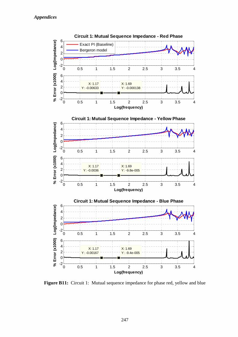
Appendices
247
Figure B11: Circuit 1: Mutual sequence impedance for phase red, yellow and blue
0 0.5 1 1.5 2 2.5 3 3.5 4-2
0
2
4
6
Log(
Impe
danc
e)
Circuit 1: Mutual Sequence Impedance - Blue Phase
0 0.5 1 1.5 2 2.5 3 3.5 4-2
0
2
4
6
X: 1.17Y: -0.00167
% E
rror
(x1
000)
Log(frequency)
X: 1.69Y: -9.4e-005
0 0.5 1 1.5 2 2.5 3 3.5 4-2
0
2
4
6
Log(
Impe
danc
e)
Circuit 1: Mutual Sequence Impedance - Yellow Phase
0 0.5 1 1.5 2 2.5 3 3.5 4-2
0
2
4
6
X: 1.17Y: -0.0036
% E
rror
(x1
000)
Log(frequency)
X: 1.69Y: -9.8e-005
0 0.5 1 1.5 2 2.5 3 3.5 4-2
0
2
4
6
Log(
Impe
danc
e)
Circuit 1: Mutual Sequence Impedance - Red Phase
0 0.5 1 1.5 2 2.5 3 3.5 4-2
0
2
4
6
X: 1.17Y: -0.00633
% E
rror
(x1
000)
Log(frequency)
X: 1.69Y: -0.000138
Exact PI (Baseline)
Bergeron model
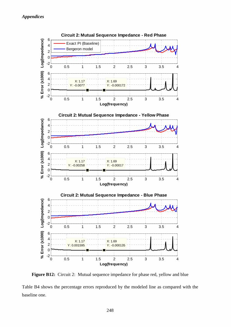
Appendices
248
Figure B12: Circuit 2: Mutual sequence impedance for phase red, yellow and blue
Table B4 shows the percentage errors reproduced by the modeled line as compared with the
baseline one.
0 0.5 1 1.5 2 2.5 3 3.5 4-2
0
2
4
6
Log(
Impe
danc
e)
Circuit 2: Mutual Sequence Impedance - Blue Phase
0 0.5 1 1.5 2 2.5 3 3.5 4-2
0
2
4
6
X: 1.17Y: 0.001595
% E
rror
(x1
000)
Log(frequency)
X: 1.69Y: -0.000135
0 0.5 1 1.5 2 2.5 3 3.5 4-2
0
2
4
6
Log(
Impe
danc
e)
Circuit 2: Mutual Sequence Impedance - Yellow Phase
0 0.5 1 1.5 2 2.5 3 3.5 4-2
0
2
4
6
X: 1.17Y: -0.00258
% E
rror
(x1
000)
Log(frequency)
X: 1.69Y: -0.00017
0 0.5 1 1.5 2 2.5 3 3.5 4-2
0
2
4
6Lo
g(Im
peda
nce)
Circuit 2: Mutual Sequence Impedance - Red Phase
0 0.5 1 1.5 2 2.5 3 3.5 4-2
0
2
4
6
X: 1.17Y: -0.0077
% E
rror
(x1
000)
Log(frequency)
X: 1.69Y: -0.000172
Exact PI (Baseline)
Bergeron model
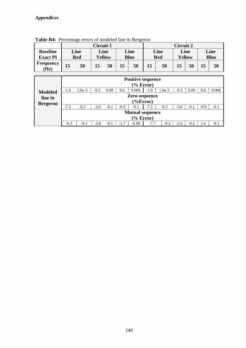
Appendices
249
Table B4: Percentage errors of modeled line in Bergeron Circuit 1 Circuit 2 Baseline Exact PI
Line Red
Line Yellow
Line Blue
Line Red
Line Yellow
Line Blue
Frequency (Hz)
15 50 15 50 15 50 15 50 15 50 15 50
Positive sequence (% Error)
-1.6 1.6e-3 -9.3 0.09 9.6 0.006 -1.6 1.6e-3 -9.3 0.09 9.6 0.006
Zero sequence (%Error)
-7.2 -0.2 -3.6 -0.1 -0.9 -0.1 -7.2 -0.2 -3.6 -0.1 -0.9 -0.1
Mutual sequence (% Error)
Modeled line in
Bergeron
-6.3 -0.1 -3.6 -0.1 -1.7 -0.09 -7.7 -0.2 -2.6 -0.2 1.6 -0.1
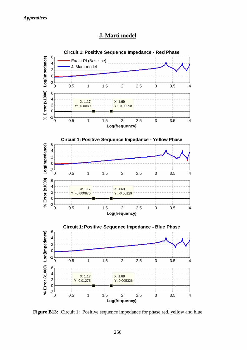
Appendices
250
J. Marti model
Figure B13: Circuit 1: Positive sequence impedance for phase red, yellow and blue
0 0.5 1 1.5 2 2.5 3 3.5 4-2
0
2
4
6
Log(
Impe
danc
e)
Circuit 1: Positive Sequence Impedance - Blue Phase
0 0.5 1 1.5 2 2.5 3 3.5 4-2
0
2
4
6
X: 1.17Y: 0.01275
% E
rror
(x1
000)
Log(frequency)
X: 1.69Y: 0.005326
0 0.5 1 1.5 2 2.5 3 3.5 4-2
0
2
4
6
Log(
Impe
danc
e)
Circuit 1: Positive Sequence Impedance - Yellow Pha se
0 0.5 1 1.5 2 2.5 3 3.5 4-2
0
2
4
6
X: 1.17Y: -0.000876
% E
rror
(x1
000)
Log(frequency)
X: 1.69Y: -0.00129
0 0.5 1 1.5 2 2.5 3 3.5 4-2
0
2
4
6
Log(
Impe
danc
e)
Circuit 1: Positive Sequence Impedance - Red Phase
0 0.5 1 1.5 2 2.5 3 3.5 4-2
0
2
4
6
X: 1.17Y: -0.0089
% E
rror
(x1
000)
Log(frequency)
X: 1.69Y: -0.00298
Exact PI (Baseline)
J. Marti model
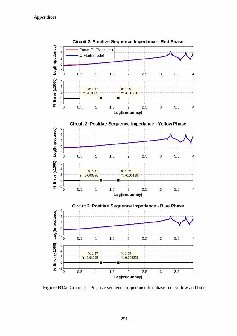
Appendices
251
Figure B14: Circuit 2: Positive sequence impedance for phase red, yellow and blue
0 0.5 1 1.5 2 2.5 3 3.5 4-2
0
2
4
6
Log(
Impe
danc
e)
Circuit 2: Positive Sequence Impedance - Yellow Pha se
0 0.5 1 1.5 2 2.5 3 3.5 4-2
0
2
4
6
X: 1.17Y: -0.000876
% E
rror
(x1
000)
Log(frequency)
X: 1.69Y: -0.00129
0 0.5 1 1.5 2 2.5 3 3.5 4-2
0
2
4
6
Log(
Impe
danc
e)
Circuit 2: Positive Sequence Impedance - Blue Phase
0 0.5 1 1.5 2 2.5 3 3.5 4-2
0
2
4
6
X: 1.17Y: 0.01275
% E
rror
(x1
000)
Log(frequency)
X: 1.69Y: 0.005326
0 0.5 1 1.5 2 2.5 3 3.5 4-2
0
2
4
6
Log(
Impe
danc
e)
Circuit 2: Positive Sequence Impedance - Red Phase
0 0.5 1 1.5 2 2.5 3 3.5 4-2
0
2
4
6
X: 1.17Y: -0.0089
% E
rror
(x1
000)
Log(frequency)
X: 1.69Y: -0.00298
Exact PI (Baseline)
J. Marti model
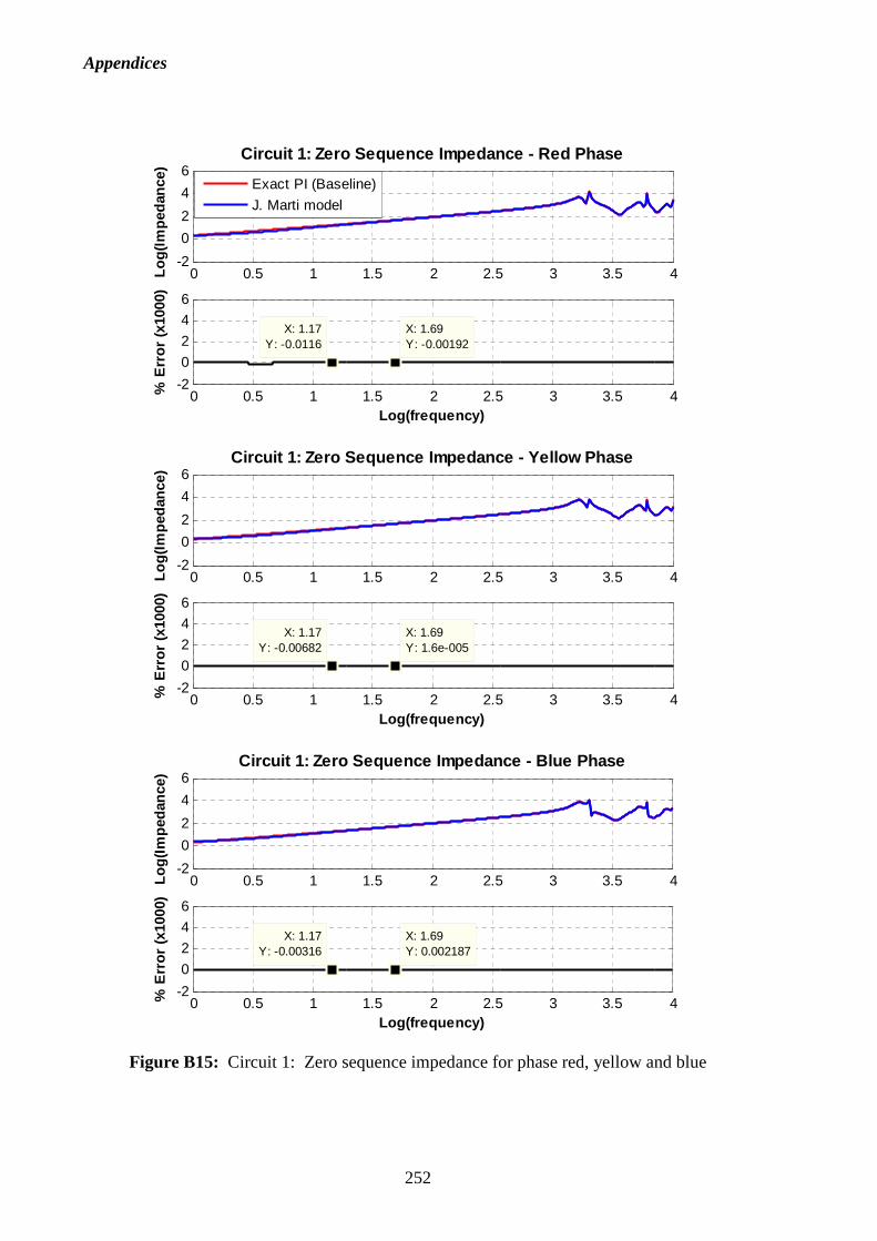
Appendices
252
Figure B15: Circuit 1: Zero sequence impedance for phase red, yellow and blue
0 0.5 1 1.5 2 2.5 3 3.5 4-2
0
2
4
6
Log(
Impe
danc
e)
Circuit 1: Zero Sequence Impedance - Blue Phase
0 0.5 1 1.5 2 2.5 3 3.5 4-2
0
2
4
6
X: 1.17Y: -0.00316
% E
rror
(x1
000)
Log(frequency)
X: 1.69Y: 0.002187
0 0.5 1 1.5 2 2.5 3 3.5 4-2
0
2
4
6
Log(
Impe
danc
e)
Circuit 1: Zero Sequence Impedance - Yellow Phase
0 0.5 1 1.5 2 2.5 3 3.5 4-2
0
2
4
6
X: 1.17Y: -0.00682
% E
rror
(x1
000)
Log(frequency)
X: 1.69Y: 1.6e-005
0 0.5 1 1.5 2 2.5 3 3.5 4-2
0
2
4
6Lo
g(Im
peda
nce)
Circuit 1: Zero Sequence Impedance - Red Phase
0 0.5 1 1.5 2 2.5 3 3.5 4-2
0
2
4
6
X: 1.17Y: -0.0116
% E
rror
(x1
000)
Log(frequency)
X: 1.69Y: -0.00192
Exact PI (Baseline)
J. Marti model
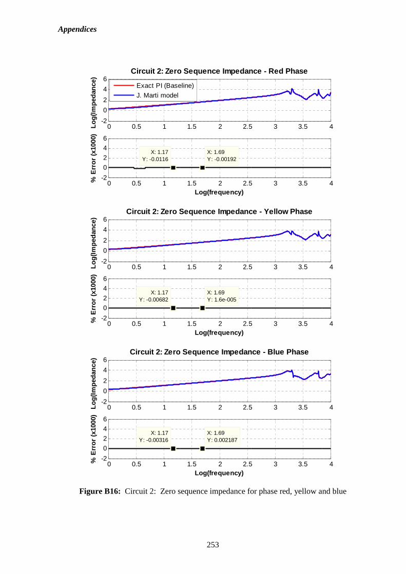
Appendices
253
Figure B16: Circuit 2: Zero sequence impedance for phase red, yellow and blue
0 0.5 1 1.5 2 2.5 3 3.5 4-2
0
2
4
6
Log(
Impe
danc
e)
Circuit 2: Zero Sequence Impedance - Blue Phase
0 0.5 1 1.5 2 2.5 3 3.5 4-2
0
2
4
6
X: 1.17Y: -0.00316
% E
rror
(x1
000)
Log(frequency)
X: 1.69Y: 0.002187
0 0.5 1 1.5 2 2.5 3 3.5 4-2
0
2
4
6
Log(
Impe
danc
e)
Circuit 2: Zero Sequence Impedance - Yellow Phase
0 0.5 1 1.5 2 2.5 3 3.5 4-2
0
2
4
6
X: 1.17Y: -0.00682
% E
rror
(x1
000)
Log(frequency)
X: 1.69Y: 1.6e-005
0 0.5 1 1.5 2 2.5 3 3.5 4-2
0
2
4
6
Log(
Impe
danc
e)
Circuit 2: Zero Sequence Impedance - Red Phase
0 0.5 1 1.5 2 2.5 3 3.5 4-2
0
2
4
6
X: 1.17Y: -0.0116
% E
rror
(x1
000)
Log(frequency)
X: 1.69Y: -0.00192
Exact PI (Baseline)
J. Marti model
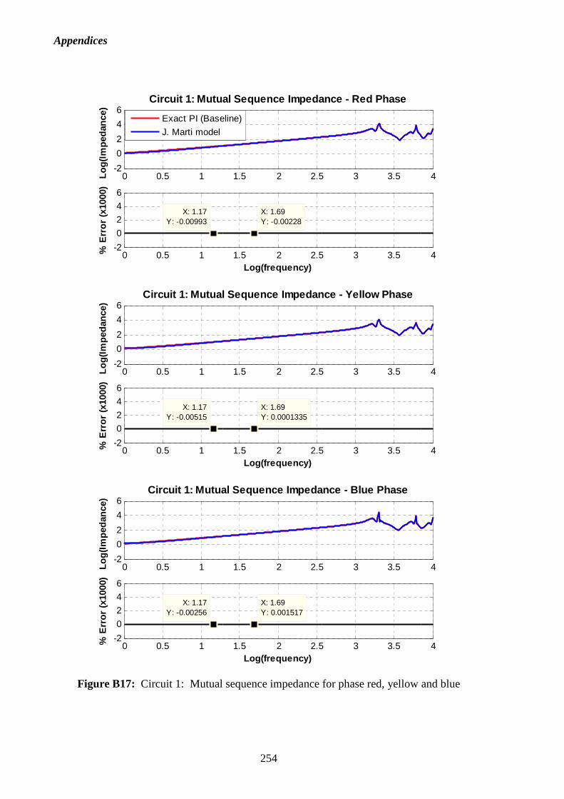
Appendices
254
Figure B17: Circuit 1: Mutual sequence impedance for phase red, yellow and blue
0 0.5 1 1.5 2 2.5 3 3.5 4-2
0
2
4
6
Log(
Impe
danc
e)
Circuit 1: Mutual Sequence Impedance - Blue Phase
0 0.5 1 1.5 2 2.5 3 3.5 4-2
0
2
4
6
X: 1.17Y: -0.00256
% E
rror
(x1
000)
Log(frequency)
X: 1.69Y: 0.001517
0 0.5 1 1.5 2 2.5 3 3.5 4-2
0
2
4
6
Log(
Impe
danc
e)
Circuit 1: Mutual Sequence Impedance - Yellow Phase
0 0.5 1 1.5 2 2.5 3 3.5 4-2
0
2
4
6
X: 1.17Y: -0.00515
% E
rror
(x1
000)
Log(frequency)
X: 1.69Y: 0.0001335
0 0.5 1 1.5 2 2.5 3 3.5 4-2
0
2
4
6Lo
g(Im
peda
nce)
Circuit 1: Mutual Sequence Impedance - Red Phase
0 0.5 1 1.5 2 2.5 3 3.5 4-2
0
2
4
6
X: 1.17Y: -0.00993
% E
rror
(x1
000)
Log(frequency)
X: 1.69Y: -0.00228
Exact PI (Baseline)
J. Marti model
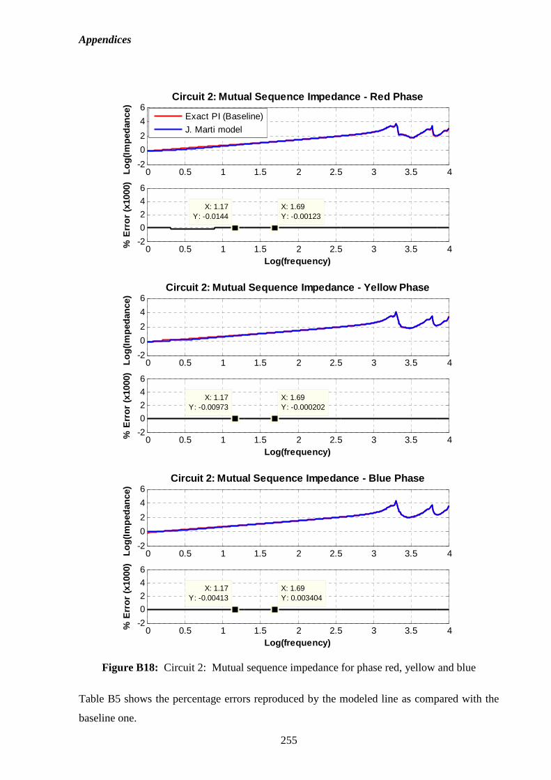
Appendices
255
Figure B18: Circuit 2: Mutual sequence impedance for phase red, yellow and blue
Table B5 shows the percentage errors reproduced by the modeled line as compared with the
baseline one.
0 0.5 1 1.5 2 2.5 3 3.5 4-2
0
2
4
6
Log(
Impe
danc
e)
Circuit 2: Mutual Sequence Impedance - Blue Phase
0 0.5 1 1.5 2 2.5 3 3.5 4-2
0
2
4
6
X: 1.17Y: -0.00413
% E
rror
(x1
000)
Log(frequency)
X: 1.69Y: 0.003404
0 0.5 1 1.5 2 2.5 3 3.5 4-2
0
2
4
6
Log(
Impe
danc
e)
Circuit 2: Mutual Sequence Impedance - Yellow Phase
0 0.5 1 1.5 2 2.5 3 3.5 4-2
0
2
4
6
X: 1.17Y: -0.00973
% E
rror
(x1
000)
Log(frequency)
X: 1.69Y: -0.000202
0 0.5 1 1.5 2 2.5 3 3.5 4-2
0
2
4
6
Log(
Impe
danc
e)
Circuit 2: Mutual Sequence Impedance - Red Phase
0 0.5 1 1.5 2 2.5 3 3.5 4-2
0
2
4
6
X: 1.17Y: -0.0144
% E
rror
(x1
000)
Log(frequency)
X: 1.69Y: -0.00123
Exact PI (Baseline)
J. Marti model
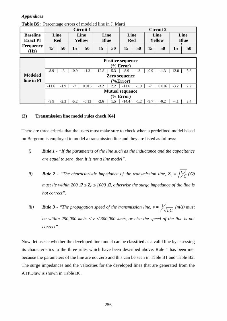
Appendices
256
Table B5: Percentage errors of modeled line in J. Marti Circuit 1 Circuit 2 Baseline Exact PI
Line Red
Line Yellow
Line Blue
Line Red
Line Yellow
Line Blue
Frequency (Hz)
15 50 15 50 15 50 15 50 15 50 15 50
Positive sequence (% Error)
-8.9 -3 -0.9 -1.3 12.8 5.3 -8.9 -3 -0.9 -1.3 12.8 5.3
Zero sequence (%Error)
-11.6 -1.9 -7 0.016 -3.2 2.2 -11.6 -1.9 -7 0.016 -3.2 2.2
Mutual sequence (% Error)
Modeled line in PI
-9.9 -2.3 -5.2 -0.13 -2.6 1.5 -14.4 -1.2 -9.7 -0.2 -4.1 3.4
(2) Transmission line model rules check [64]
There are three criteria that the users must make sure to check when a predefined model based
on Bergeron is employed to model a transmission line and they are listed as follows:
i) Rule 1 - “If the parameters of the line such as the inductance and the capacitance
are equal to zero, then it is not a line model”.
ii) Rule 2 - “The characteristic impedance of the transmission line, cLZ C= (Ω)
must lie within 200 Ω ≤ Zc ≤ 1000 Ω, otherwise the surge impedance of the line is
not correct”.
iii) Rule 3 - “The propagation speed of the transmission line, 1vLC
= (m/s) must
be within 250,000 km/s ≤ v ≤ 300,000 km/s, or else the speed of the line is not
correct”.
Now, let us see whether the developed line model can be classified as a valid line by assessing
its characteristics to the three rules which have been described above. Rule 1 has been met
because the parameters of the line are not zero and this can be seen in Table B1 and Table B2.
The surge impedances and the velocities for the developed lines that are generated from the
ATPDraw is shown in Table B6.
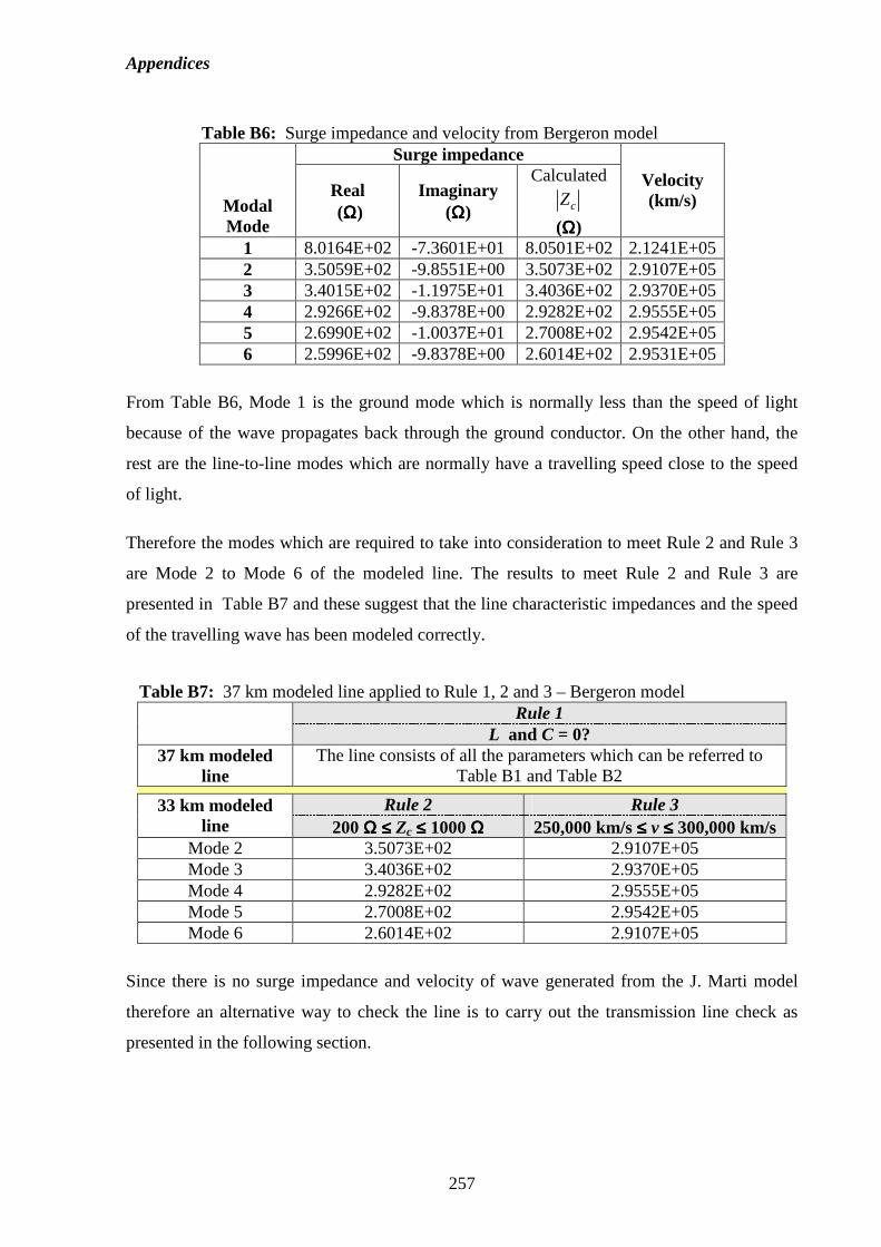
Appendices
257
Table B6: Surge impedance and velocity from Bergeron model Surge impedance
Modal Mode
Real (ΩΩΩΩ)
Imaginary (ΩΩΩΩ)
Calculated
cZ
(ΩΩΩΩ)
Velocity (km/s)
1 8.0164E+02 -7.3601E+01 8.0501E+02 2.1241E+05 2 3.5059E+02 -9.8551E+00 3.5073E+02 2.9107E+05 3 3.4015E+02 -1.1975E+01 3.4036E+02 2.9370E+05 4 2.9266E+02 -9.8378E+00 2.9282E+02 2.9555E+05 5 2.6990E+02 -1.0037E+01 2.7008E+02 2.9542E+05 6 2.5996E+02 -9.8378E+00 2.6014E+02 2.9531E+05
From Table B6, Mode 1 is the ground mode which is normally less than the speed of light
because of the wave propagates back through the ground conductor. On the other hand, the
rest are the line-to-line modes which are normally have a travelling speed close to the speed
of light.
Therefore the modes which are required to take into consideration to meet Rule 2 and Rule 3
are Mode 2 to Mode 6 of the modeled line. The results to meet Rule 2 and Rule 3 are
presented in Table B7 and these suggest that the line characteristic impedances and the speed
of the travelling wave has been modeled correctly.
Table B7: 37 km modeled line applied to Rule 1, 2 and 3 – Bergeron model Rule 1
L and C = 0? 37 km modeled
line The line consists of all the parameters which can be referred to
Table B1 and Table B2
Rule 2 Rule 3 33 km modeled line 200 ΩΩΩΩ ≤≤≤≤ Zc ≤≤≤≤ 1000 ΩΩΩΩ 250,000 km/s ≤≤≤≤ v ≤≤≤≤ 300,000 km/s
Mode 2 3.5073E+02 2.9107E+05 Mode 3 3.4036E+02 2.9370E+05 Mode 4 2.9282E+02 2.9555E+05 Mode 5 2.7008E+02 2.9542E+05 Mode 6 2.6014E+02 2.9107E+05
Since there is no surge impedance and velocity of wave generated from the J. Marti model
therefore an alternative way to check the line is to carry out the transmission line check as
presented in the following section.
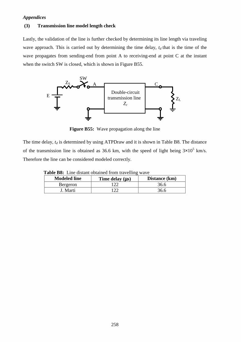
Appendices
258
(3) Transmission line model length check
Lastly, the validation of the line is further checked by determining its line length via traveling
wave approach. This is carried out by determining the time delay, td that is the time of the
wave propagates from sending-end from point A to receiving-end at point C at the instant
when the switch SW is closed, which is shown in Figure B55.
Figure B55: Wave propagation along the line
The time delay, td is determined by using ATPDraw and it is shown in Table B8. The distance
of the transmission line is obtained as 36.6 km, with the speed of light being 3×10⁵ km/s.
Therefore the line can be considered modeled correctly.
Table B8: Line distant obtained from travelling wave Modeled line Time delay (µµµµs) Distance (km)
Bergeron 122 36.6 J. Marti 122 36.6
Double-circuit transmission line
Zc
ZS
ZL
SW
A C
E
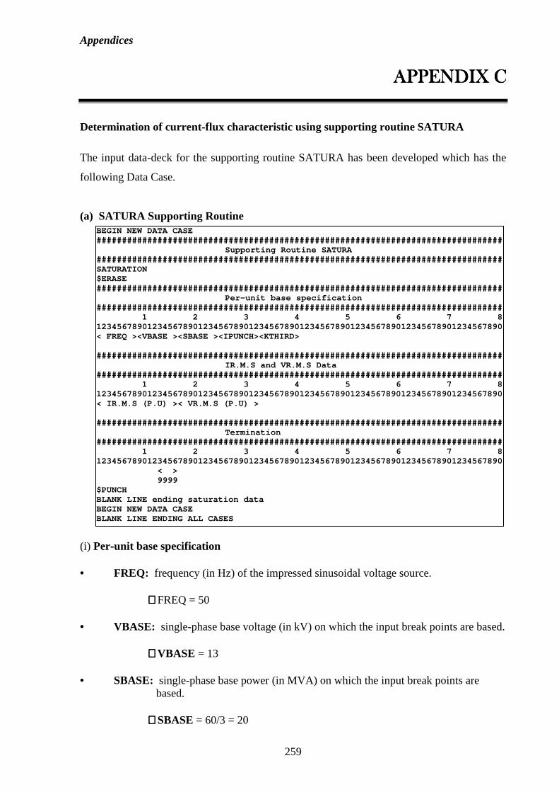
Appendices
259
APPENDIX CAPPENDIX CAPPENDIX CAPPENDIX C
Determination of current-flux characteristic using supporting routine SATURA
The input data-deck for the supporting routine SATURA has been developed which has the
following Data Case.
(a) SATURA Supporting Routine
(i) Per-unit base specification • FREQ: frequency (in Hz) of the impressed sinusoidal voltage source.
∴∴∴∴FREQ = 50
• VBASE: single-phase base voltage (in kV) on which the input break points are based. ∴∴∴∴VBASE = 13
• SBASE: single-phase base power (in MVA) on which the input break points are based.
∴∴∴∴SBASE = 60/3 = 20
BEGIN NEW DATA CASE ################################################################################ Supporting Routine SATURA ################################################################################ SATURATION $ERASE ################################################################################ Per-unit base specification ################################################################################ 1 2 3 4 5 6 7 8 12345678901234567890123456789012345678901234567890123456789012345678901234567890 < FREQ ><VBASE ><SBASE ><IPUNCH><KTHIRD> ################################################################################ IR.M.S and VR.M.S Data ################################################################################ 1 2 3 4 5 6 7 8 12345678901234567890123456789012345678901234567890123456789012345678901234567890 < IR.M.S (P.U) >< VR.M.S (P.U) > ################################################################################ Termination ################################################################################ 1 2 3 4 5 6 7 8 12345678901234567890123456789012345678901234567890123456789012345678901234567890 < > 9999 $PUNCH BLANK LINE ending saturation data BEGIN NEW DATA CASE BLANK LINE ENDING ALL CASES
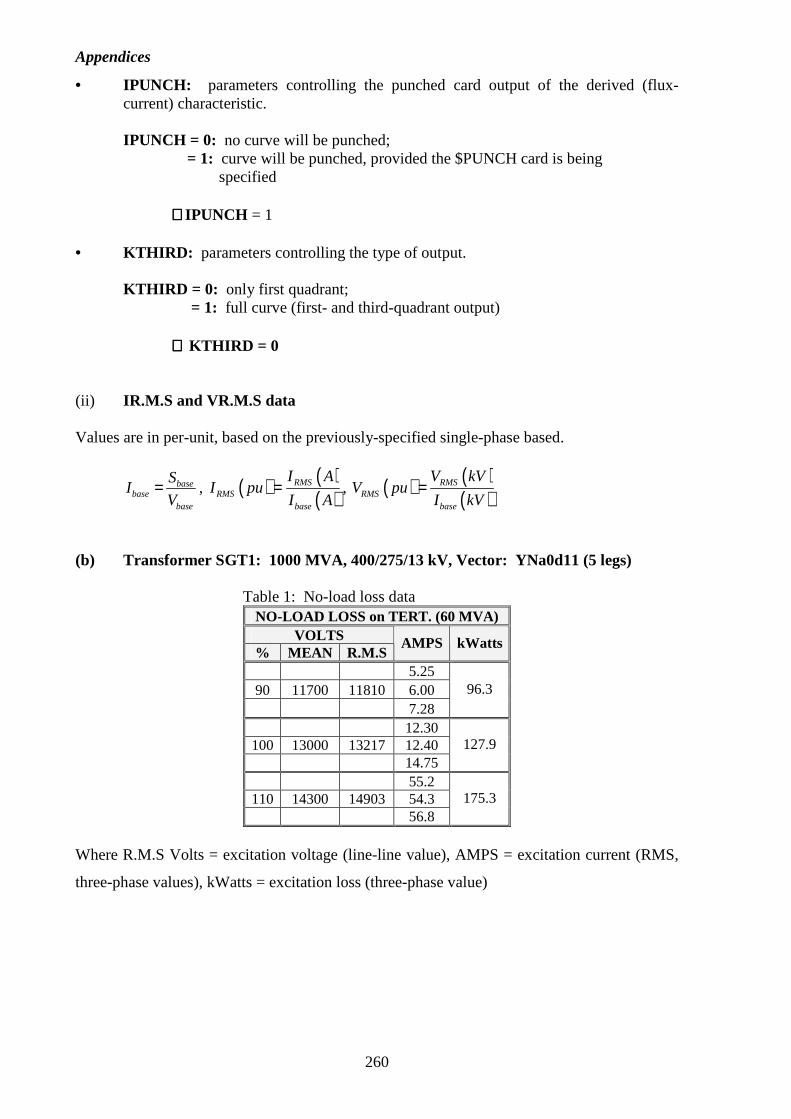
Appendices
260
• IPUNCH: parameters controlling the punched card output of the derived (flux-current) characteristic.
IPUNCH = 0: no curve will be punched; = 1: curve will be punched, provided the $PUNCH card is being specified
∴∴∴∴IPUNCH = 1
• KTHIRD: parameters controlling the type of output.
KTHIRD = 0: only first quadrant; = 1: full curve (first- and third-quadrant output)
∴∴∴∴ KTHIRD = 0 (ii) IR.M.S and VR.M.S data Values are in per-unit, based on the previously-specified single-phase based.
basebase
base
SI
V= , ( ) ( )
( )RMS
RMSbase
I AI pu
I A= , ( ) ( )
( )RMS
RMSbase
V kVV pu
I kV=
(b) Transformer SGT1: 1000 MVA, 400/275/13 kV, Vector: YNa0d11 (5 legs) Table 1: No-load loss data
NO-LOAD LOSS on TERT. (60 MVA) VOLTS
% MEAN R.M.S AMPS kWatts
5.25 90 11700 11810 6.00 7.28
96.3
12.30 100 13000 13217 12.40
14.75 127.9
55.2 110 14300 14903 54.3
56.8 175.3
Where R.M.S Volts = excitation voltage (line-line value), AMPS = excitation current (RMS,
three-phase values), kWatts = excitation loss (three-phase value)
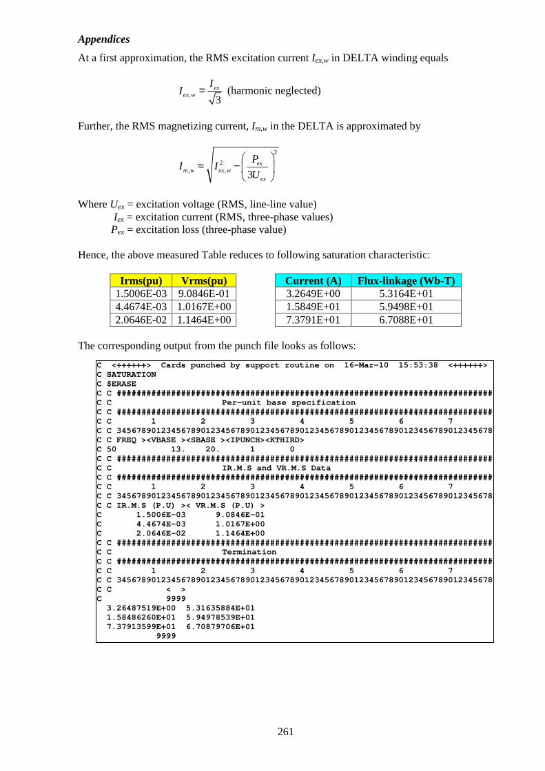
Appendices
261
At a first approximation, the RMS excitation current Iex,w in DELTA winding equals
,3ex
ex w
II = (harmonic neglected)
Further, the RMS magnetizing current, Im,w in the DELTA is approximated by
2
2, , 3
exm w ex w
ex
PI I
U
≈ −
Where Uex = excitation voltage (RMS, line-line value) Iex = excitation current (RMS, three-phase values) Pex = excitation loss (three-phase value) Hence, the above measured Table reduces to following saturation characteristic:
Irms(pu) Vrms(pu) Current (A) Flux-linkage (Wb-T) 1.5006E-03 9.0846E-01 3.2649E+00 5.3164E+01 4.4674E-03 1.0167E+00 1.5849E+01 5.9498E+01 2.0646E-02 1.1464E+00 7.3791E+01 6.7088E+01
The corresponding output from the punch file looks as follows:
C <++++++> Cards punched by support routine on 16-Mar-10 15:53:38 <++++++> C SATURATION C $ERASE C C ############################################################################ C C Per-unit base specification C C ############################################################################ C C 1 2 3 4 5 6 7 C C 3456789012345678901234567890123456789012345678901234567890123456789012345678 C C FREQ ><VBASE ><SBASE ><IPUNCH><KTHIRD> C 50 13. 20. 1 0 C C ############################################################################ C C IR.M.S and VR.M.S Data C C ############################################################################ C C 1 2 3 4 5 6 7 C C 3456789012345678901234567890123456789012345678901234567890123456789012345678 C C IR.M.S (P.U) >< VR.M.S (P.U) > C 1.5006E-03 9.0846E-01 C 4.4674E-03 1.0167E+00 C 2.0646E-02 1.1464E+00 C C ############################################################################ C C Termination C C ############################################################################ C C 1 2 3 4 5 6 7 C C 3456789012345678901234567890123456789012345678901234567890123456789012345678 C C < > C 9999 3.26487519E+00 5.31635884E+01 1.58486260E+01 5.94978539E+01 7.37913599E+01 6.70879706E+01 9999
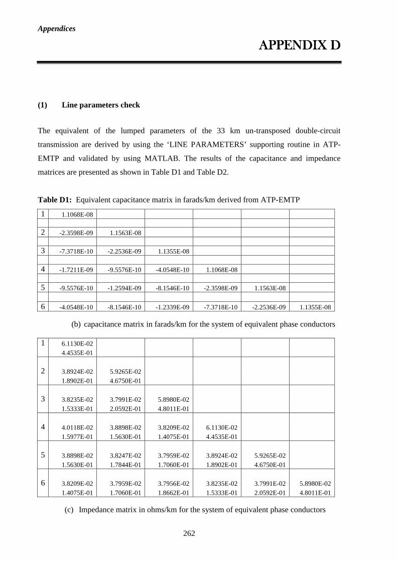
Appendices
262
APPENDIX DAPPENDIX DAPPENDIX DAPPENDIX D
(1) Line parameters check
The equivalent of the lumped parameters of the 33 km un-transposed double-circuit
transmission are derived by using the ‘LINE PARAMETERS’ supporting routine in ATP-
EMTP and validated by using MATLAB. The results of the capacitance and impedance
matrices are presented as shown in Table D1 and Table D2.
Table D1: Equivalent capacitance matrix in farads/km derived from ATP-EMTP
1 1.1068E-08
2 -2.3598E-09 1.1563E-08
3 -7.3718E-10 -2.2536E-09 1.1355E-08
4 -1.7211E-09 -9.5576E-10 -4.0548E-10 1.1068E-08
5 -9.5576E-10 -1.2594E-09 -8.1546E-10 -2.3598E-09 1.1563E-08 6 -4.0548E-10 -8.1546E-10 -1.2339E-09 -7.3718E-10 -2.2536E-09 1.1355E-08
(b) capacitance matrix in farads/km for the system of equivalent phase conductors
1 6.1130E-02 4.4535E-01 2 3.8924E-02 5.9265E-02 1.8902E-01 4.6750E-01 3 3.8235E-02 3.7991E-02 5.8980E-02 1.5333E-01 2.0592E-01 4.8011E-01 4 4.0118E-02 3.8898E-02 3.8209E-02 6.1130E-02 1.5977E-01 1.5630E-01 1.4075E-01 4.4535E-01 5 3.8898E-02 3.8247E-02 3.7959E-02 3.8924E-02 5.9265E-02 1.5630E-01 1.7844E-01 1.7060E-01 1.8902E-01 4.6750E-01 6 3.8209E-02 3.7959E-02 3.7956E-02 3.8235E-02 3.7991E-02 5.8980E-02 1.4075E-01 1.7060E-01 1.8662E-01 1.5333E-01 2.0592E-01 4.8011E-01
(c) Impedance matrix in ohms/km for the system of equivalent phase conductors
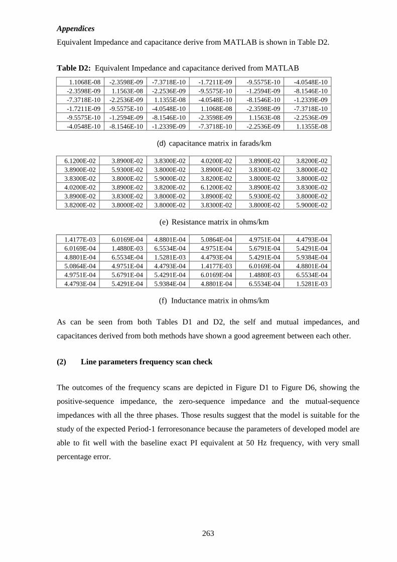
Appendices
263
Equivalent Impedance and capacitance derive from MATLAB is shown in Table D2.
Table D2: Equivalent Impedance and capacitance derived from MATLAB
1.1068E-08 -2.3598E-09 -7.3718E-10 -1.7211E-09 -9.5575E-10 -4.0548E-10 -2.3598E-09 1.1563E-08 -2.2536E-09 -9.5575E-10 -1.2594E-09 -8.1546E-10 -7.3718E-10 -2.2536E-09 1.1355E-08 -4.0548E-10 -8.1546E-10 -1.2339E-09 -1.7211E-09 -9.5575E-10 -4.0548E-10 1.1068E-08 -2.3598E-09 -7.3718E-10 -9.5575E-10 -1.2594E-09 -8.1546E-10 -2.3598E-09 1.1563E-08 -2.2536E-09 -4.0548E-10 -8.1546E-10 -1.2339E-09 -7.3718E-10 -2.2536E-09 1.1355E-08
(d) capacitance matrix in farads/km
6.1200E-02 3.8900E-02 3.8300E-02 4.0200E-02 3.8900E-02 3.8200E-02 3.8900E-02 5.9300E-02 3.8000E-02 3.8900E-02 3.8300E-02 3.8000E-02 3.8300E-02 3.8000E-02 5.9000E-02 3.8200E-02 3.8000E-02 3.8000E-02 4.0200E-02 3.8900E-02 3.8200E-02 6.1200E-02 3.8900E-02 3.8300E-02 3.8900E-02 3.8300E-02 3.8000E-02 3.8900E-02 5.9300E-02 3.8000E-02 3.8200E-02 3.8000E-02 3.8000E-02 3.8300E-02 3.8000E-02 5.9000E-02
(e) Resistance matrix in ohms/km
1.4177E-03 6.0169E-04 4.8801E-04 5.0864E-04 4.9751E-04 4.4793E-04 6.0169E-04 1.4880E-03 6.5534E-04 4.9751E-04 5.6791E-04 5.4291E-04 4.8801E-04 6.5534E-04 1.5281E-03 4.4793E-04 5.4291E-04 5.9384E-04 5.0864E-04 4.9751E-04 4.4793E-04 1.4177E-03 6.0169E-04 4.8801E-04 4.9751E-04 5.6791E-04 5.4291E-04 6.0169E-04 1.4880E-03 6.5534E-04 4.4793E-04 5.4291E-04 5.9384E-04 4.8801E-04 6.5534E-04 1.5281E-03
(f) Inductance matrix in ohms/km
As can be seen from both Tables D1 and D2, the self and mutual impedances, and
capacitances derived from both methods have shown a good agreement between each other.
(2) Line parameters frequency scan check
The outcomes of the frequency scans are depicted in Figure D1 to Figure D6, showing the
positive-sequence impedance, the zero-sequence impedance and the mutual-sequence
impedances with all the three phases. Those results suggest that the model is suitable for the
study of the expected Period-1 ferroresonance because the parameters of developed model are
able to fit well with the baseline exact PI equivalent at 50 Hz frequency, with very small
percentage error.
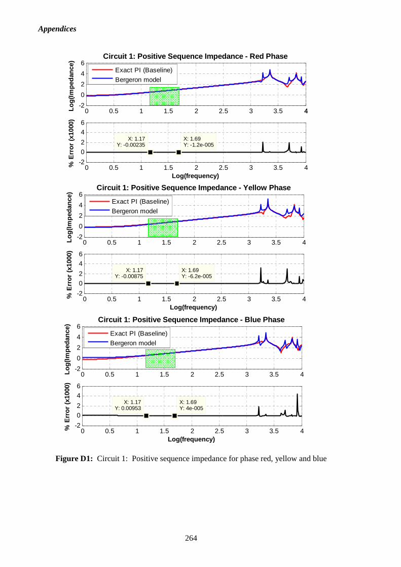
Appendices
264
Figure D1: Circuit 1: Positive sequence impedance for phase red, yellow and blue
0 0.5 1 1.5 2 2.5 3 3.5 44-2
0
2
4
6Lo
g(Im
peda
nce)
Circuit 1: Positive Sequence Impedance - Red Phase
0 0.5 1 1.5 2 2.5 3 3.5 4-2
0
2
4
6
X: 1.17Y: -0.00235
% E
rror
(x1
000)
Log(frequency)
X: 1.69Y: -1.2e-005
Exact PI (Baseline)
Bergeron model
0 0.5 1 1.5 2 2.5 3 3.5 4-2
0
2
4
6
Log(
Impe
danc
e)
Circuit 1: Positive Sequence Impedance - Yellow Pha se
0 0.5 1 1.5 2 2.5 3 3.5 4-2
0
2
4
6
X: 1.17Y: -0.00875
% E
rror
(x1
000)
Log(frequency)
X: 1.69Y: -6.2e-005
Exact PI (Baseline)
Bergeron model
0 0.5 1 1.5 2 2.5 3 3.5 4-2
0
2
4
6
Log(
Impe
danc
e)
Circuit 1: Positive Sequence Impedance - Blue Phase
0 0.5 1 1.5 2 2.5 3 3.5 4-2
0
2
4
6
X: 1.17Y: 0.00953
% E
rror
(x1
000)
Log(frequency)
X: 1.69Y: 4e-005
Exact PI (Baseline)
Bergeron model
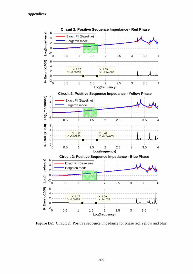
Appendices
265
Figure D2: Circuit 2: Positive sequence impedance for phase red, yellow and blue
0 0.5 1 1.5 2 2.5 3 3.5 4-2
0
2
4
66
Log(
Impe
danc
e)
Circuit 2: Positive Sequence Impedance - Red Phase
0 0.5 1 1.5 2 2.5 3 3.5 4-2
0
2
4
6
X: 1.17Y: -0.00235
% E
rror
(x1
000)
Log(frequency)
X: 1.69Y: -1.2e-005
Exact PI (Baseline)
Bergeron model
0 0.5 1 1.5 2 2.5 3 3.5 4-2
0
2
4
6
Log(
Impe
danc
e)
Circuit 2: Positive Sequence Impedance - Yellow Pha se
0 0.5 1 1.5 2 2.5 3 3.5 4-2
0
2
4
6
X: 1.17Y: -0.00875
% E
rror
(x1
000)
Log(frequency)
X: 1.69Y: -6.2e-005
Exact PI (Baseline)
Bergeron model
0 0.5 1 1.5 2 2.5 3 3.5 4-2
0
2
4
6
Log(
Impe
danc
e)
Circuit 2: Positive Sequence Impedance - Blue Phase
0 0.5 1 1.5 2 2.5 3 3.5 4-2
0
2
4
6
X: 1.17Y: 0.00953
% E
rror
(x1
000)
Log(frequency)
X: 1.69Y: 4e-005
Exact PI (Baseline)
Bergeron model
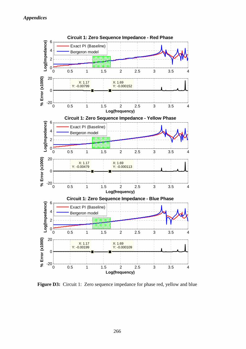
Appendices
266
Figure D3: Circuit 1: Zero sequence impedance for phase red, yellow and blue
0 0.5 1 1.5 2 2.5 3 3.5 40
2
4
6Lo
g(Im
peda
nce)
Circuit 1: Zero Sequence Impedance - Red Phase
0 0.5 1 1.5 2 2.5 3 3.5 4-20
0
20X: 1.17
Y: -0.00799
% E
rror
(x1
000)
Log(frequency)
X: 1.69Y: -0.000152
Exact PI (Baseline)
Bergeron model
0 0.5 1 1.5 2 2.5 3 3.5 40
2
4
6
Log(
Impe
danc
e)
Circuit 1: Zero Sequence Impedance - Yellow Phase
0 0.5 1 1.5 2 2.5 3 3.5 4-20
0
20X: 1.17
Y: -0.00479
% E
rror
(x1
000)
Log(frequency)
X: 1.69Y: -0.000113
Exact PI (Baseline)
Bergeron model
0 0.5 1 1.5 2 2.5 3 3.5 40
2
4
6
Log(
Impe
danc
e)
Circuit 1: Zero Sequence Impedance - Blue Phase
0 0.5 1 1.5 2 2.5 3 3.5 4-20
0
20X: 1.17
Y: -0.00199
% E
rror
(x1
000)
Log(frequency)
X: 1.69Y: -0.000109
Exact PI (Baseline)
Bergeron model
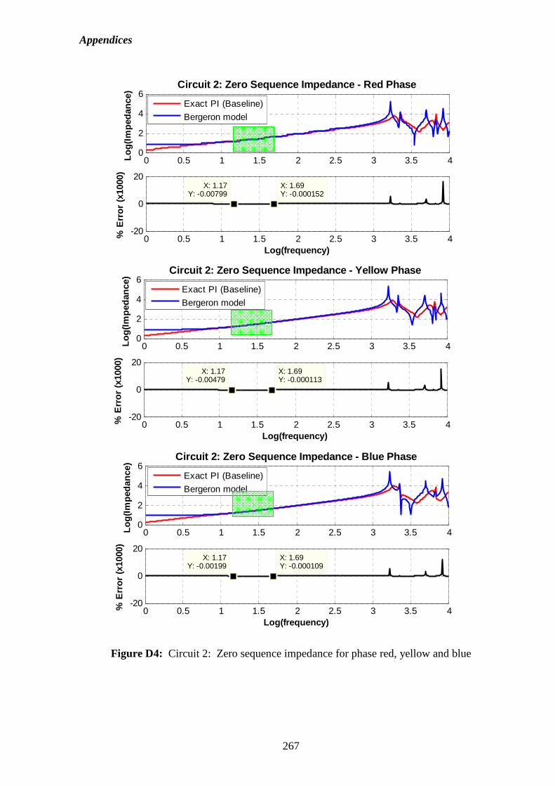
Appendices
267
Figure D4: Circuit 2: Zero sequence impedance for phase red, yellow and blue
0 0.5 1 1.5 2 2.5 3 3.5 40
2
4
6
Log(
Impe
danc
e)
Circuit 2: Zero Sequence Impedance - Red Phase
0 0.5 1 1.5 2 2.5 3 3.5 4-20
0
20X: 1.17
Y: -0.00799
% E
rror
(x1
000)
Log(frequency)
X: 1.69Y: -0.000152
Exact PI (Baseline)
Bergeron model
0 0.5 1 1.5 2 2.5 3 3.5 40
2
4
6
Log(
Impe
danc
e)
Circuit 2: Zero Sequence Impedance - Yellow Phase
0 0.5 1 1.5 2 2.5 3 3.5 4-20
0
20X: 1.17
Y: -0.00479
% E
rror
(x1
000)
Log(frequency)
X: 1.69Y: -0.000113
Exact PI (Baseline)
Bergeron model
0 0.5 1 1.5 2 2.5 3 3.5 40
2
4
6
Log(
Impe
danc
e)
Circuit 2: Zero Sequence Impedance - Blue Phase
0 0.5 1 1.5 2 2.5 3 3.5 4-20
0
20X: 1.17
Y: -0.00199
% E
rror
(x1
000)
Log(frequency)
X: 1.69Y: -0.000109
Exact PI (Baseline)
Bergeron model
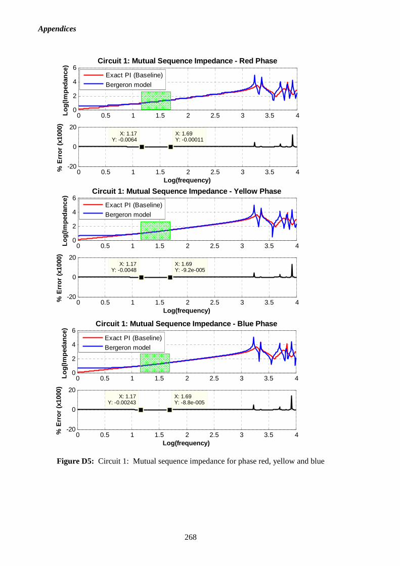
Appendices
268
Figure D5: Circuit 1: Mutual sequence impedance for phase red, yellow and blue
0 0.5 1 1.5 2 2.5 3 3.5 40
2
4
6Lo
g(Im
peda
nce)
Circuit 1: Mutual Sequence Impedance - Red Phase
0 0.5 1 1.5 2 2.5 3 3.5 4-20
0
20X: 1.17
Y: -0.0064
% E
rror
(x1
000)
Log(frequency)
X: 1.69Y: -0.00011
Exact PI (Baseline)
Bergeron model
0 0.5 1 1.5 2 2.5 3 3.5 40
2
4
6
Log(
Impe
danc
e)
Circuit 1: Mutual Sequence Impedance - Yellow Phase
0 0.5 1 1.5 2 2.5 3 3.5 4-20
0
20X: 1.17
Y: -0.0048
% E
rror
(x1
000)
Log(frequency)
X: 1.69Y: -9.2e-005
Exact PI (Baseline)
Bergeron model
0 0.5 1 1.5 2 2.5 3 3.5 40
2
4
6
Log(
Impe
danc
e)
Circuit 1: Mutual Sequence Impedance - Blue Phase
0 0.5 1 1.5 2 2.5 3 3.5 4-20
0
20X: 1.17
Y: -0.00243
% E
rror
(x1
000)
Log(frequency)
X: 1.69Y: -8.8e-005
Exact PI (Baseline)
Bergeron model
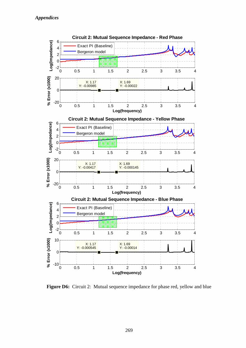
Appendices
269
Figure D6: Circuit 2: Mutual sequence impedance for phase red, yellow and blue
0 0.5 1 1.5 2 2.5 3 3.5 4-2
0
2
4
6
Log(
Impe
danc
e)
Circuit 2: Mutual Sequence Impedance - Red Phase
0 0.5 1 1.5 2 2.5 3 3.5 4-20
0
20X: 1.17
Y: -0.00985
% E
rror
(x1
000)
Log(frequency)
X: 1.69Y: -0.00022
Exact PI (Baseline)
Bergeron model
0 0.5 1 1.5 2 2.5 3 3.5 4-2
0
2
4
6
Log(
Impe
danc
e)
Circuit 2: Mutual Sequence Impedance - Yellow Phase
0 0.5 1 1.5 2 2.5 3 3.5 4-20
0
20X: 1.17
Y: -0.00417
% E
rror
(x1
000)
Log(frequency)
X: 1.69Y: -0.000145
Exact PI (Baseline)
Bergeron model
0 0.5 1 1.5 2 2.5 3 3.5 4-2
0
2
4
6
Log(
Impe
danc
e)
Circuit 2: Mutual Sequence Impedance - Blue Phase
0 0.5 1 1.5 2 2.5 3 3.5 4-10
0
10X: 1.17
Y: -0.000545
% E
rror
(x1
000)
Log(frequency)
X: 1.69Y: -0.00014
Exact PI (Baseline)
Bergeron model
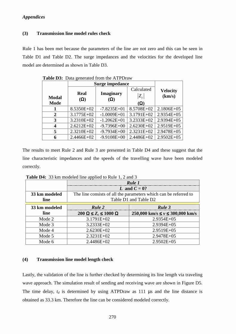
Appendices
270
(3) Transmission line model rules check
Rule 1 has been met because the parameters of the line are not zero and this can be seen in
Table D1 and Table D2. The surge impedances and the velocities for the developed line
model are determined as shown in Table D3.
Table D3: Data generated from the ATPDraw Surge impedance
Modal Mode
Real (ΩΩΩΩ)
Imaginary (ΩΩΩΩ)
Calculated
cZ
(ΩΩΩΩ)
Velocity (km/s)
1 8.5350E+02 -7.8235E+01 8.5708E+02 2.1806E+05 2 3.1775E+02 -1.0009E+01 3.1791E+02 2.9354E+05 3 3.2310E+02 -1.2062E+01 3.2333E+02 2.9394E+05 4 2.6212E+02 -9.7396E+00 2.6230E+02 2.9519E+05 5 2.3210E+02 -9.7934E+00 2.3231E+02 2.9478E+05 6 2.4466E+02 -9.9108E+00 2.4486E+02 2.9502E+05
The results to meet Rule 2 and Rule 3 are presented in Table D4 and these suggest that the
line characteristic impedances and the speeds of the travelling wave have been modeled
correctly.
Table D4: 33 km modeled line applied to Rule 1, 2 and 3 Rule 1
L and C = 0? 33 km modeled
line The line consists of all the parameters which can be referred to
Table D1 and Table D2
Rule 2 Rule 3 33 km modeled line 200 ΩΩΩΩ ≤≤≤≤ Zc ≤≤≤≤ 1000 ΩΩΩΩ 250,000 km/s ≤≤≤≤ v ≤≤≤≤ 300,000 km/s
Mode 2 3.1791E+02 2.9354E+05 Mode 3 3.2333E+02 2.9394E+05 Mode 4 2.6230E+02 2.9519E+05 Mode 5 2.3231E+02 2.9478E+05 Mode 6 2.4486E+02 2.9502E+05
(4) Transmission line model length check
Lastly, the validation of the line is further checked by determining its line length via traveling
wave approach. The simulation result of sending and receiving wave are shown in Figure D5.
The time delay, td is determined by using ATPDraw as 111 µs and the line distance is
obtained as 33.3 km. Therefore the line can be considered modeled correctly.
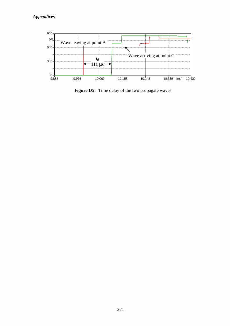
Appendices
271
Figure D5: Time delay of the two propagate waves
9.885 9.976 10.067 10.158 10.248 10.339 10.430[ms]0
300
600
900
[V]
td 111 µµµµs
Wave leaving at point A
Wave arriving at point C