arX
iv:1
208.
2219
v1 [
cond
-mat
.mtr
l-sc
i] 1
0 A
ug 2
012
Ferroelectric control of magnetization in La1−xSrxMnO3
manganites: A first-principles study
Hanghui Chen1,3 and Sohrab Ismail-Beigi1,2,3
1Department of Physics, Yale University,
New Haven, Connecticut, 06511, USA
2Department of Applied Physics, Yale University,
New Haven, Connecticut, 06511, USA
3Center for Research on Interface Structures and Phenomena (CRISP),
Yale University, New Haven, CT 06511, USA
(Dated: December 23, 2013)
Abstract
We present a first-principles study on the interface between perovskite ferroelectrics (PbTiO3)
and conducting magnetic manganites (La1−xSrxMnO3). We show that by switching the ferroelec-
tric polarization, additional carriers are accumulated or depleted at the interfacial region of the
manganite and that this change in carrier density can modify the magnetic spin configuration of
the interfacial Mn, which is consistent with the experimentally observed anomalously large change
in the magnetization. We also describe an unexpected purely interfacial phenomenon whereby the
ferroelectric polarization of the interfacial region changes the magnetic energetics — a degree of
freedom not present in bulk manganites. Theoretically, we show the the ground-state magnetic
structure depends sensitively on the precise choice of Hubbard U parameter within the widely-
used DFT+U class of exchange correlation functionals. We provide a simple Ising-like model that
explains the evolution of the magnetic structure with U in tandem with a discussion of various
different ways in which one might try to choose an appropriate U parameter.
1

I. INTRODUCTION
Multiferroics have been one of the most intensively studied materials during the past
decade [1, 2]. The coexistence of more than one order parameter in a single phase and their
coupling may open new routes to the next generation of electronic devices. For instance,
the possibility of controlling magnetization via external electric fields may find promising
applications in spintronics. The origin of magnetoelectric multiferroicity lies in a nonzero
magnetoelectric coupling which may occur due to many different mechanisms (for recent
reviews, see [3, 4]). The magnetic properties of an intrinsic bulk magnetoelectric, of which
Cr2O3 is a prototype, can be modulated by an external field through the change of the
magnetic cations’ displacement relative to anions [5]. Extrinsic magnetoelectric couplings
are typically mediated by strain: in composites of piezomagnetic materials combined with
electrostrictive materials, external fields modulate the electric polarization, as well as the
shape of the piezoelectric. This change in turn induces strain of the magnetic components
and modifies the magnetization in the magnetostrictive material [6].
However, although these bulk mechanisms are well understood, the magnitude of mag-
netoelectric couplings in bulk materials is generally small [7], impeding their applications in
electronic devices. Moving away from bulk materials, artificial heterostructures such as in-
terfaces are promising candidates for realizing or even engineering magnetoelectric couplings.
Recently, a variety of mechanisms were proposed to induce magnetoelectric coupling at inter-
faces. At ferromagnet/ferroelectric interfaces, the interfacial bond length can be altered by
the presence of ferroelectric polarization, for example in Fe/BaTiO3 [8], Co2MnSi/BaTiO3
[9] and Fe3O4/BaTiO3 [10]. Another mechanism is to apply an external field and induce
magnetization mediated by free screening carriers accumulated at ferromagnetic/dielectric
interfaces, for example SrRuO3/SrTiO3 [11]. A more complex but intriguing mechanism
was recently described theoretically and experimentally [12, 13] at ferroelectric/conducting
magnetic manganite interfaces. Our work focuses on this last class of systems, because the
coupling between ferroelectric polarization and magnetization not only is of great impor-
tance in fundemental sciences, but also finds very promising applications in memory devices
[14, 15].
At a ferroelectric/manganite interface, the presence of the ferroelectric polarization causes
screening charges to appear at the interface due to accumulation or depletion of carriers in the
2

interfacial region. Much like SrRuO3/SrTiO3 interfaces, the magnetization of the interfacial
atoms can be enhanced due to the modification of carrier density around the interface
because the magnetic moment of the atoms depends on the doping level (provided that the
manganite is in the ferromagnetic phase). What is different in the ferroelectric/manganite
system is that the accumulation of carriers not only changes the magnetic moment but
can lead to an interfacial ferromagnetic-to-antiferromagnetic transition which reverses the
directions of the moments and thus to a much larger magnetoelectric coupling. The work
of Ref. [12] studied a representative heterostructure: BaTiO3/La1−xBaxMnO3 with x = 0.5.
For bulk La1−xSrxMnO3, x = 0.5 is at the critical doping level separating ferromagnetic and
antiferromagnetic phases, so the system is highly susceptible to magnetic changes with small
changes of doping. What was found is that when the ferroelectric polarization is flipped, the
magnetic moment of the Mn atoms in the second unit cell away from the interface is reversed.
We note that the result is somewhat unintuitive as the carrier doping density is highest
in the first layer at the interface which is most susceptible to change of magnetic phase.
Experiments on the Pb(Ti0.8Zr0.2)O3/La1−xSrxMnO3 are performed for x = 0.2 [13] which
is quite far from the boundary: a priori it is not clear whether enough screening charges can
accumulate to drive the system over the magnetic phase transition. The experiments find a
large magneto-electric coupling which is interpreted to originate from a spin-flip in the first
unit cell of the manganite closest to the interface [13].
In this work, we comprehensively study this proposed magnetoelectric phenomenon
at the ferroelectric/manganite interface using first-principles calculations. We choose
PbTiO3/La1−xSrxMnO3 as our prototype for computational convenience. Although the ex-
periments use Pb(Ti0.8Zr0.2)O3 as the ferroelectric [13] in order to reduce leakage currents,
the key role of the ferroelectric is to induce screening charges due to its surface polarization,
and we believe the compositional details are secondary. For the La1−xSrxMnO3 thin film,
we choose the nominal hole doping to be x = 0.2 (unless otherwise specified) in order to
directly compare to experiment [13].
The original contributions of this paper are the following. (i) We are able to show that
even though the manganite film has a low nominal doping of x = 0.2, the ferroelectric field
effects can sufficiently change the carrier density to induce a magnetic transition at the inter-
face. However, the precise ground-state magnetic structure of the interface (e.g., no spin-flip,
spin-flip in first Mn layer, spin-flip in second Mn layer) depends sensitively on the choice
3
of exchange correlation functionals and specifically the value of the Hubbard U parameter
in the DFT+U approach. (ii) We clarify the physical reasons of the sensitivity based on a
simple Ising-like nearest-neighbor model using bulk-derived parameters that well describes
the computed dependences. (iii) We describe an unexpected purely interfacial effect that
significantly modifies the energies of magnetic states at the interface: the ferroelectric polar-
ization propagates into the first few manganite layers and the resulting rumplings of atomic
layers are responsible for the modifications. This degree of freedom is not present in the
bulk and potentially represents a further degree of freedom that can be exploited to modify
and engineer material properties at oxide interfaces. (iv) We show that various approaches
to find an appropriate U produce significantly different U values, some of which do poorly
when used to compute results that compare to bulk properties of manganites; empiricism
in the choice of U is an unfortunate necessity for manganites using state-of-the-art ab initio
methods. (v) In the process of this work, we develop an alternative method for counting
electrons on the Mn atoms in La1−xSrxMnO3 thin films that is directly based on the electron
density instead of the standard and widely used method based on projecting onto Lowdin
or atomic-like orbitals [16]. With this method, we can quantify the carrier distribution as a
function of ferroelectric polarization and calculate the layer-resolved effective hole doping.
The method is generally applicable to half-metallic oxide films.
The remainder of the paper is organized as follows. We discuss computational details
in Section II. We first study the magnetic phase transition of bulk La1−xSrxMnO3 in Sec-
tion IIIA. A discussion of Hubbard U for bulk La1−xSrxMnO3 is presented in Section IIIB.
The charge modulation at the interface is studied in Section IVB and Section IVC is de-
voted to the discussion of spin modulation at the interface. We conclude in Section V. A
number of appendices contain further technical details.
II. COMPUTATIONAL DETAILS
Our calculations are performed using density functional theory within the ab initio su-
percell plane-wave approach [17], with the code PWscf in the Quantum-ESPRESSO package
[38]. We employ ultrasoft pseudopotentials [18]. The semicore states and reference config-
uration of each element are shown in Table I. We use the local spin density approximation
(LSDA) [19] for the exchange correlation functional as well as the Hubbard U correction
4

TABLE I: The semicore states and reference configurations of our pseudopotentials. The cut-off
radii are in units of Bohr.
Atom Reference valence states rsc rpc rdc
Pb 5d106s26p2 2.5 2.5 2.3
Ti 3s23p63d14s2 1.8 1.8 1.8
Sr 4s24p65s2 2.0 1.8 2.0
La 5s25p65d16s1.56p0.5 2.2 2.0 2.2
Mn 3s23p63d54s2 2.0 2.0 2.0
Pt 5d96s16p0 1.0 1.0 1.2
O 2s22p4 1.3 1.3 –
method (LSDA+U) [20] to account for some of the strong electronic correlations on the
localized d orbitals of Mn atoms. The plane wave basis energy cutoff and charge cutoff are
35 Ry and 280 Ry, respectively. We use a Gaussian smearing width of 5 mRy when sampling
the Brillouin zone. For bulk La1−xSrxMnO3, the k-grid sampling of the Brillouin zone is
20× 20× 20 per formula unit. For interface calculations, the k-grid sampling is 20× 20× 2
where the z-axis is orthogonal to the interface. For variable cell relaxations, the convergence
threshold for pressure is 0.5 Kbar. For atom relaxations, the convergence threshold for ev-
ery force component is 26 meV/A. We have checked the convergence in total energies and
structural parameters by further increasing the k-point sampling and reducing the stress
and force threshold, and observe no significant differences in key physical observables.
The A-site La1−xSrx alloying is treated by the virtual crystal approximation [21, 22].
Appendix A describes tests on the accuracy of the virtual crystal approximation for our
system: the results are highly satisfactory and consistent with earlier observations [23]
5

FIG. 1: (Color online) a) 20-atom unit cell of Pnma La1−xSrxMnO3. b) Experimental phase dia-
gram of La1−xSrxMnO3. ‘CI’ means canted insulating. ‘FI’ means ferromagnetic insulating. ‘FM’
means ferromagnetic metallic. ‘AFM’ means antiferromagnetic metallic. ‘PI’ means paramagnetic
insulating. ‘PM’ means paramagnetic metallic. The phase boundary of the ferromagnetic to A-
type antiferromagnetic phase transition at low temperatures is highlighted by the bold dashed line.
The panel b) is reproduced with permission from Ref. [27]. Copyright 2006 Institute of Physics
Publishing.
III. BULK MANGANITES
A. Phase transition of magnetic ordering
Since, as we will show, the magnetic properties of PbTiO3/La1−xSrxMnO3 interface can
be understood qualitatively in terms of bulk La1−xSrxMnO3, we start the discussion with the
phase diagram of bulk La1−xSrxMnO3 under different conditions. The parent compound of
La1−xSrxMnO3 is LaMnO3 which is an A-type antiferromagnetic Mott insulator [24]. Bulk
LaMnO3 has strong Jahn-Teller and GdFeO3 distortions with Pnma symmetry [25] and its
primitive cell is of size c(2× 2)× 2 in units of the cubic perovskite. The smallest unit cell of
LaMnO3 has four formula units (20 atoms), as is illustrated in Fig. 1a. Chemically doping
LaMnO3 with Sr induces holes on the Mn d-orbitals, leading to conduction and various
6

0 0.2 0.4 0.6 0.8 1
Hole doping x
-120
-60
0
60
120
∆E/M
n (m
eV)
0 0.2 0.4 0.6 0.8 1
Hole doping x
-120
-60
0
60
120
∆E/M
n (m
eV) U = 0 eV
U = 1 eVU = 2 eV
0 0.2 0.4 0.6 0.8 1
Hole doping x
-120
-60
0
60
120
∆E/M
n (m
eV)
unstrainedSrTiO3-strained
0 0.2 0.4 0.6 0.8 1
Hole doping x
-180
-120
-60
0
60
∆E/M
n (m
eV)
a b
c d
PnmaP4
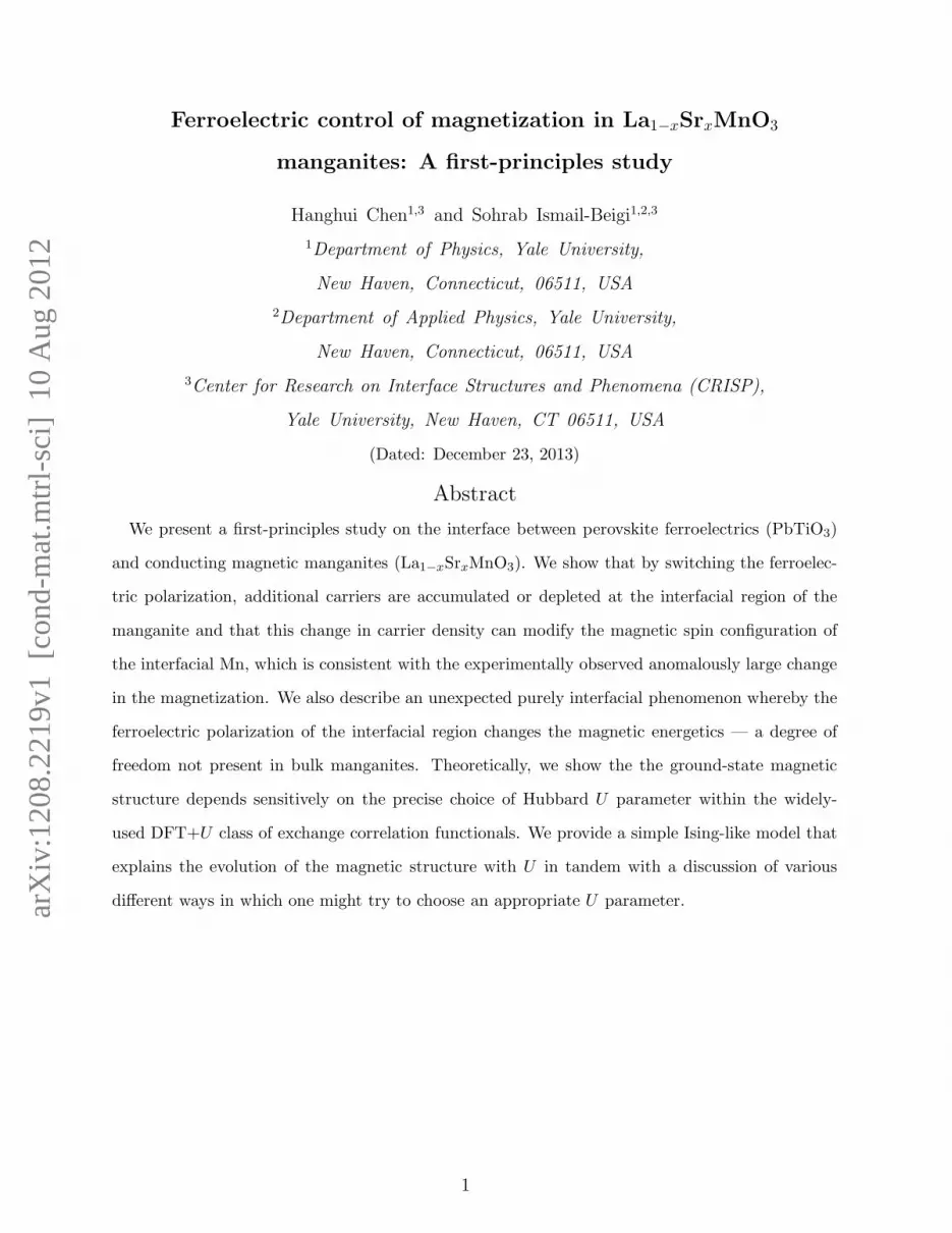
FIG. 2: (Color online) Phase diagram of bulk Pnma La1−xSrxMnO3. ∆E is defined in Eq. (1).
Above zero, the ground state is ferromagnetic and below zero it is A-type antiferromagnetic. a)
Hole doping dependence within LSDA. b) Hubbard U dependence. c) Strain dependence. d)
Structural distortion dependence.
magnetic orderings. Fig. 1b shows the experimental phase diagram of bulk La1−xSrxMnO3.
A ferromagnetic to A-type antiferromagnetic phase transition occurs around x =0.5 doping,
which is highlighted by the bold dashed line in Fig. 1b. For a random alloy distribution,
we assume that bulk La1−xSrxMnO3 has the same symmetry as LaMnO3 (Pnma). In DFT
simulations, we replace La with the fictitious atom La1−xSrx in the virtual crystal approxi-
mation and calculate the energy difference between ferromagnetic ordering (F ) and A-type
antiferromagnetic ordering (A) as a function of doping x.
∆E = E(A)− E(F ) (1)
In addition to the doping dependence x, we also study the effect of strain, structural distor-
tions and Hubbard U on the magnetic transition of bulk La1−xSrxMnO3.
7

1. Doping dependence
Fig. 2a shows a representative bulk phase diagram of La1−xSrxMnO3 as a function of
doping x. The calculation is performed in the LSDA (i.e. Hubbard U=0). DFT-LSDA
reproduces the ferromagnetic-to-antiferromagnetic phase transition that is observed in ex-
periment. The doping dependence can be understood as follows: the ferromagnetic ordering
is stablized by the double exchange mechanism which relies on the hopping of the lone eg
electrons among the Mn3+ ions [26]. With the increasing hole doping x, the itinerant elec-
trons (i.e. Mn3+ ions) are drained and the hopping processes are suppressed. Therefore
the double exchange mechanism becomes less operative and the ferromagnetic ordering gets
more unstable as x is increased. We need to point out that in the experimental phase dia-
gram for x < 0.1, La1−xSrxMnO3 is a spin-canted insulator (a magnetic structure close to
A-type antiferromagnetic ordering but the magnetic moment is not exactly cancelled due to
weak spin-canting) [27]. As x increases to 0.2, there is an insulating-to-metallic transition
and the appearance of the ferromagnetic ordering which is not reproduced in the DFT-LSDA
calculation, since the LSDA ground state is metallic in the whole doping range. Turning on
the Hubbard U does not change the metallicity of ferromagnetic La1−xSrxMnO3. We argue
that even though LSDA or LSDA+U is not accurate enough to reproduce the spin-canted
ground state at very low doping nor the insulating-to-metallic transition around x ≃ 0.2,
it correctly produces the metallic ferromagnetic to metallic antiferromagnetic phase transi-
tion at larger x, which is the key to understanding the spin-modified magnetic structure of
manganites in the presence of ferroelectrics.
2. Hubbard U dependence
Fig. 2b shows a comparison of LSDA and LSDA+U calculations for bulk La1−xSrxMnO3.
The ferromagnetic-to-antiferromagnetic phase transition is well reproduced in both LSDA
and LSDA+U calculations, but the transition point, i.e. the critical hole density where the
ground state changes magnetic ordering, depends on the value of the Hubbard U . With an
increasing U , the transition point moves to larger doping values while the overall features
of the transition remain unchanged. The Hubbard U dependence originates as follows:
antiferromagnetism is favored by the superexchange mechanism which involves the virtual
8
hopping of electrons between low and high energy sites with the same spin [28]. A larger
U increases the energy splitting and thus the virtual hopping is suppressed. Therefore the
superexchange mechanism is suppressed as U increases, and the antiferromagnetic ordering
accordingly becomes less stable, resulting in the upward shift of phase transition curve
(favoring ferromagnetism). Empirically in order to correctly locate the transition point at
the experimental value of x ≃ 0.5, we need a Hubbard U in the range of 1 eV< U <2 eV in
the LSDA+U approximation (as illustrated in Fig. 2b).
3. Strain dependence
Since the La1−xSrxMnO3 thin film is grown coherently on an SrTiO3 substrate, we also
study the phase diagram of SrTiO3-strained La1−xSrxMnO3 and compare it with unstrained
bulk La1−xSrxMnO3 in Fig. 2c. La1−xSrxMnO3 in the whole doping range is under weak
tensile strain (within 1%) when on an SrTiO3 substrate. Tensile (compressive) strain re-
moves the degeneracy of Mn eg orbitals and favors dx2−y2 (d3z2−r2) orbitals due to the change
of crystal field [29]. Based on the double exchange mechanism, ferromagnetism is isotropic
with equal hoppings between Mn atoms along x, y and z directions. A-type antiferromag-
netism is ferromagnetic in-plane and alternates its spin orientation layer by layer along the
out-of-plane axis [30]. Due to the tensile strain, the occupancy of d3d2−r2 is lowered and
the hopping between Mn atoms becomes essentially two-dimensional, suppressing ferromag-
netism. Therefore with tensile strain, ferromagnetism is destablized and the whole transition
curve is shifted downwards (favoring A-type antiferromagnetic ordering) as seen in Fig. 2c.
4. Structural distortions
Distortions away from cubic symmetry play a crucial role in the magnetism of manganites
[31]. Bulk La1−xSrxMnO3 has complicated structural distortions with Pnma symmetry (the
unit cell is c(2 × 2) × 2 with 20 atoms). However, we also theoretically study ‘artificial’
La1−xSrxMnO3 with only tetragonal distortions (the symmetry is P4 and the unit cell is
1× 1× 2). The main reason we consider the high symmetry phase (P4) and compare it to
the low symmetry structure (Pnma) is computational: the P4 symmetry allows for the use
of a smaller 1 × 1 interface unit cell which allows for simulation of much thicker films and
9

substrates. Therefore we need to understand the main differences, if any, between the two
phases for what follows below. In addition, a comparison allows us to elucidate the role of
structural distortions.
Fig. 2d shows a representative phase diagram versus doping for both Pnma
La1−xSrxMnO3 and P4 La1−xSrxMnO3 in the LSDA approximation. To understand these
results, we begin with the fact that the effective hopping matrix element t between neigh-
bouring Mn atoms depends on the Mn-O-Mn bond angle [32]. In the P4 case, the bond
angle is 180◦ and the hopping is maximized, while in the Pnma case, the bond angle is
smaller than 180◦ and the hopping is reduced. The double exchange mechanism depends
linearly on this effective hopping matrix element t, while the superexchange mechanism low-
ers the energy of antiferromagnetism by ∝ t2 from second-order perturbation theory [32].
Therefore as we increase the hopping matrix element t, superexhange is more significantly
enhanced than double exchange, thus favoring antiferromagnetism. Compared to the Pnma
case, the P4 case has a larger effective hopping and the transition curve is shifted to favor
antiferromagnetic ordering. This trend holds for both LSDA and LSDA+U calculations.
Therefore, phenomenologically we can map Pnma La1−xSrxMnO3 to P4 La1−xSrxMnO3 by
choosing an appropriate Hubbard U . We find that in order to reproduce the ferromagnetic-
to-antiferromagnetic transition around x ≃ 0.5 in the P4 case, we need 3 eV < U < 4 eV.
By comparison, to locate the correct transition point for Pnma La1−xSrxMnO3, U must be
in the range of 1 eV < U < 2 eV (see Fig. 2b).
B. Choosing Hubbard U
The DFT+U approach is commonly used to study manganites [25]. However, neither the
choice of Hubbard U value nor the method of choosing it is unanimous. Obviously, one can
choose U based on purely empirical considerations that use experimental data: for example,
we showed above that when 1 eV < U < 2 eV, LSDA+U can correctly locate the experimen-
tal critical doping density (x = 0.5) separating ferromagnetic and antiferromagnetic phases
for bulk Pnma manganites. Below, we discuss two other reasonable-seeming methods one
might consider to determine U . The approaches yield very different values of U that tend not
to overlap and do not do well in comparison to experiment. In our opinion, unfortunately
there is no reliable way to determine U in a theoretical a priori manner. Our opinion is that
10

a single-particle approach such as DFT+U will generally run into difficulties in describing
strongly correlated system such as manganites, so that empiricism in choosing parameters
is a necessary fact of life. Since the magnetic properties depend sensitively on the value of
U , in our mind a more fruitful approach is to study a wide range of U to understand the
trends versus U and especially why the trends take the form that they do instead of trying
to make specific predictions based on some particular choice of U . (The U dependence of
bulk manganite and ferroelectric/manganite interfaces are discussed in Sections IIIA 2 and
IVC, respectively.)
1. Bulk LaMnO3
First we may ask what U value properly describes the parent material: bulk LaMnO3.
This value then may be a reasonable guess for the doped manganites. Taking into account
the structural distortions by using a c(2 × 2) × 2 unit cell [25] and by relaxing all degrees
of freedom, we calculate the total energies of different magnetic orderings and find their
energy sequence as a function of U . The result is shown in Table II. In particular, we
explicitly list ∆E, defined by Eq. (1) in the table. We can see that within a wide range
of U , the ground state is not the experimentally observed A-type antiferromagnet, nor is
there any tendency that ferromagnetism could yield to antiferromagnetism in the large U
limit. However, reproducing the insulating properties of the A-type antiferromagnetic phase
requires U ≥ 4 eV.
We note that one can perform self-consistent calculations on bulk LaMnO3 using the
experimental lattice parameters and atomic coordinates. It is possible to stabilize an insu-
lating A-type ground-state for U ≤ 1 eV, as shown in Table III. For a comprehensive study
of bulk LaMnO3 studied with a variety of exchange correlation functionals and basis sets,
please refer to [33] and references therein. Unfortunately, the reproduction for the correct
ground state when using experimental structures is not of great value for our study: we have
a non bulk-like interfacial system where the in-plane lattice constants are fixed via epitaxy
to a substrate and all remaining degrees of freedom must be relaxed, so we must return
to Table II. It would seem the best choice is either U = 0 (which stabilizes the incorrect
ground-state by the least energy) or U > 4 (which makes the A-type phase insulating). As
shown above, neither choice is satisfactory in reproducing the experimental x ≃ 0.5 phase
11
boundary for the doped manganites.
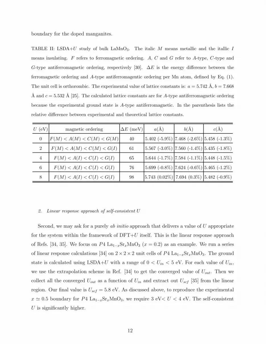
TABLE II: LSDA+U study of bulk LaMnO3. The italic M means metallic and the itallic I
means insulating. F refers to ferromagnetic ordering. A, C and G refer to A-type, C-type and
G-type antiferromagnetic ordering, respectively [30]. ∆E is the energy difference between the
ferromagnetic ordering and A-type antiferromagentic ordering per Mn atom, defined by Eq. (1).
The unit cell is orthorombic. The experimental value of lattice constants is: a = 5.742 A, b = 7.668
A and c = 5.532 A [25]. The calculated lattice constants are for A-type antiferromagnetic ordering
because the experimental ground state is A-type antiferromagnetic. In the parenthesis lists the
relative difference between experimental and theoretical lattice constants.
U (eV) magnetic ordering ∆E (meV) a(A) b(A) c(A)
0 F (M) < A(M) < C(M) < G(M) 40 5.402 (-5.9%) 7.468 (-2.6%) 5.458 (-1.3%)
2 F (M) < A(M) < C(M) < G(I) 61 5.567 (-3.0%) 7.560 (-1.4%) 5.435 (-1.8%)
4 F (M) < A(I) < C(I) < G(I) 65 5.644 (-1.7%) 7.584 (-1.1%) 5.448 (-1.5%)
6 F (M) < A(I) < C(I) < G(I) 76 5.699 (-0.8%) 7.624 (-0.6%) 5.465 (-1.2%)
8 F (M) < A(I) < C(I) < G(I) 98 5.743 (0.02%) 7.694 (0.3%) 5.482 (-0.9%)
2. Linear response approach of self-consistent U
Second, we may ask for a purely ab initio approach that delivers a value of U appropriate
for the system within the framework of DFT+U itself. This is the linear response approach
of Refs. [34, 35]. We focus on P4 La1−xSrxMnO3 (x = 0.2) as an example. We run a series
of linear response calculations [34] on 2× 2× 2 unit cells of P4 La1−xSrxMnO3. The ground
state is calculated using LSDA+U with a range of 0 < Uin < 5 eV. For each value of Uin,
we use the extrapolation scheme in Ref. [34] to get the converged value of Uout. Then we
collect all the converged Uout as a function of Uin and extract out Uscf [35] from the linear
region. Our final value is Uscf = 5.8 eV. As discussed above, to reproduce the experimental
x ≃ 0.5 boundary for P4 La1−xSrxMnO3, we require 3 eV< U < 4 eV. The self-consistent
U is significantly higher.
12
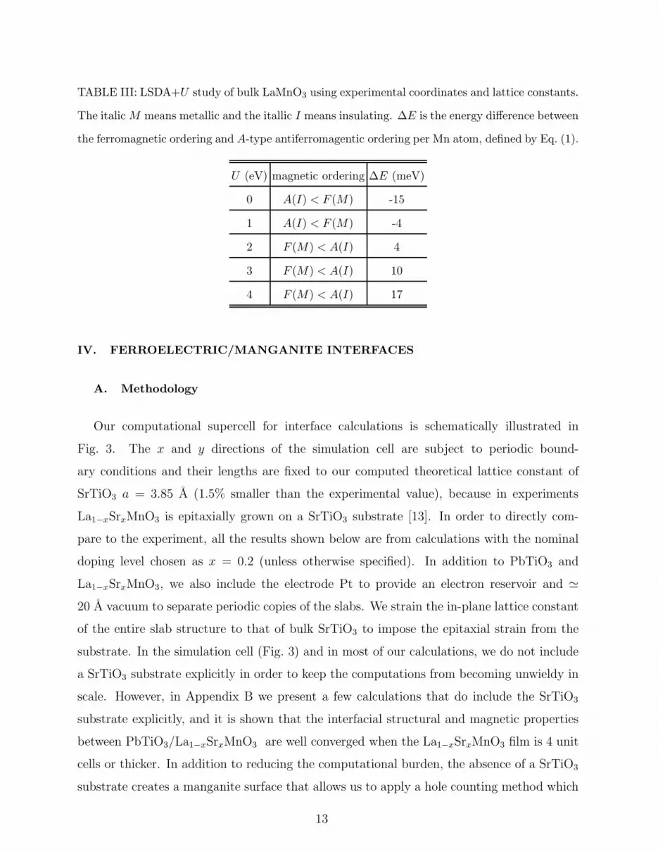
TABLE III: LSDA+U study of bulk LaMnO3 using experimental coordinates and lattice constants.
The italic M means metallic and the itallic I means insulating. ∆E is the energy difference between
the ferromagnetic ordering and A-type antiferromagentic ordering per Mn atom, defined by Eq. (1).
U (eV) magnetic ordering ∆E (meV)
0 A(I) < F (M) -15
1 A(I) < F (M) -4
2 F (M) < A(I) 4
3 F (M) < A(I) 10
4 F (M) < A(I) 17
IV. FERROELECTRIC/MANGANITE INTERFACES
A. Methodology
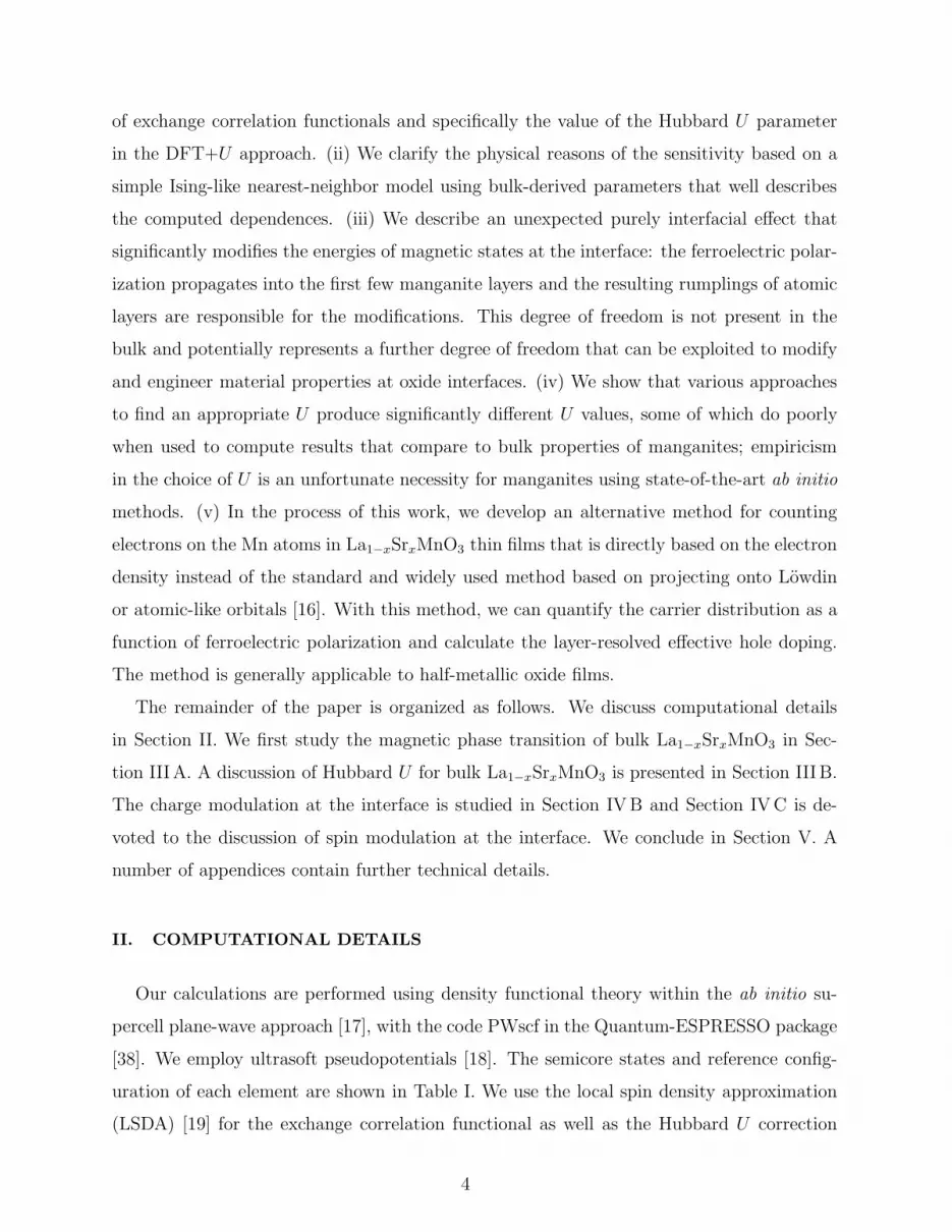
Our computational supercell for interface calculations is schematically illustrated in
Fig. 3. The x and y directions of the simulation cell are subject to periodic bound-
ary conditions and their lengths are fixed to our computed theoretical lattice constant of
SrTiO3 a = 3.85 A (1.5% smaller than the experimental value), because in experiments
La1−xSrxMnO3 is epitaxially grown on a SrTiO3 substrate [13]. In order to directly com-
pare to the experiment, all the results shown below are from calculations with the nominal
doping level chosen as x = 0.2 (unless otherwise specified). In addition to PbTiO3 and
La1−xSrxMnO3, we also include the electrode Pt to provide an electron reservoir and ≃
20 A vacuum to separate periodic copies of the slabs. We strain the in-plane lattice constant
of the entire slab structure to that of bulk SrTiO3 to impose the epitaxial strain from the
substrate. In the simulation cell (Fig. 3) and in most of our calculations, we do not include
a SrTiO3 substrate explicitly in order to keep the computations from becoming unwieldy in
scale. However, in Appendix B we present a few calculations that do include the SrTiO3
substrate explicitly, and it is shown that the interfacial structural and magnetic properties
between PbTiO3/La1−xSrxMnO3 are well converged when the La1−xSrxMnO3 film is 4 unit
cells or thicker. In addition to reducing the computational burden, the absence of a SrTiO3
substrate creates a manganite surface that allows us to apply a hole counting method which
13

FIG. 3: (Color online) Illustration of the computational supercell. The dashed line highlights the
PbO/MnO2 interface. The whole structure is coherently strained to the lattice constant of SrTiO3.
Vacuum ≃ 20 A thick is introduced to separate periodic copies. An XO (X=La/Sr) atomic layer
faces the vacuum.
can much more accurately calculate the hole spatial distribution than the use of Lowdin
orbitals [16] (see Appendix C for details). Since the SrTiO3 substrate is typically TiO2-
terminated and the manganites are in principle deposited stoichiometrically and epitaxially
on the SrTiO3, the resulting ferroelectric/manganite interface is taken to be PbO/MnO2.
Using the Berry phase method [36], we find that SrTiO3-strained PbTiO3 has bulk po-
larization 0.74 C/m2. For the two different directions of ferroelectric polarization, we define
two distinct states: the accumulation state in which extra holes are induced into the in-
terfacial La1−xSrxMnO3 and depletion state in which extra electrons are induced into the
interfacial La1−xSrxMnO3 (i.e., holes are driven out). One unit cell of PbTiO3 in the interior
is fixed to the bulk ferroelectric PbTiO3 positions, an choice that simulates the behavior of
a thick PbTiO3 film. All remaining atomic coordinates in the slab are relaxed. We need to
mention that our choice of boundary condition on ferroelectrics is consistent with the exper-
iment [13] in which a thick film of 250 nm Pb(Zr0.2Ti0.8)O3 is deposited on La1−xSrxMnO3.
However, the boundary condition on the ferroelectric could be different, depending on the
experiments to be studied. For example, in Ref. [15], three unit cells of BaTiO3 adjacent
to a La0.7Sr0.3MnO3 film are fully relaxed without the presence of Pt electron reservior, in
order to simulate the ultra-thin ferroelectrics used in other experiments [14]. Interestingly,
the results of magnetoelectric coupling in Ref. [15] are consistent with ours, described below.
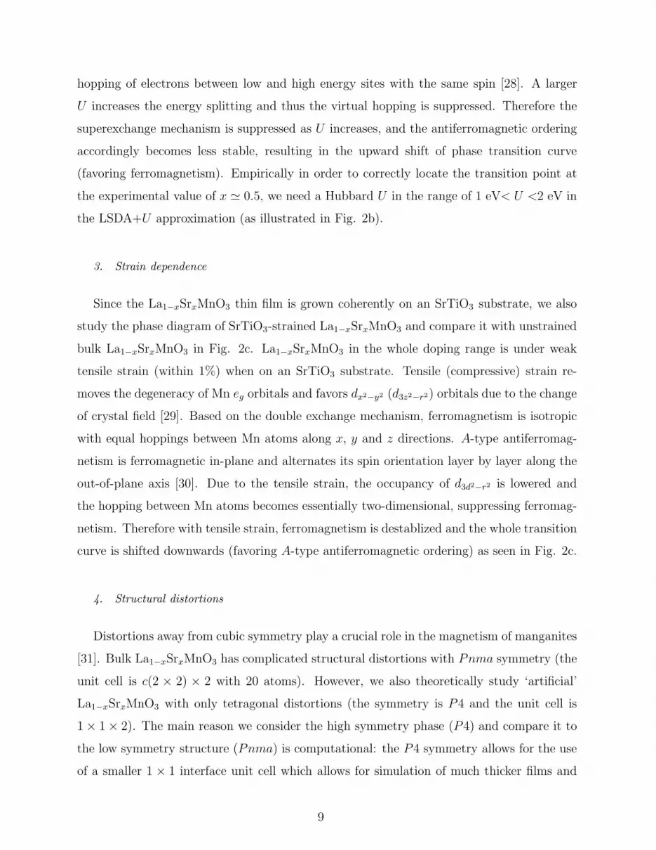
In Fig. 4, we show the cation-oxygen z-axis displacements of a representative PbTiO3
14

-0.5
-0.25
0
0.25
0.5
Cat
ion-
oxyg
en d
ispl
acm
ent (
Å)
PbO PbO PbO PbO PbOTiO 2TiO 2
TiO 2TiO 2
Pt
MnO
2
accumulationparaelectricdepletion
FIG. 4: (Color online) Cation-oxygen displacements along z-axis for the PbTiO3 film inside the
Pt/PbTiO3/La1−xSrxMnO3 heterostructures. The two purple solid lines highlights the one unit
cell of PbTiO3 that is fixed to bulk positions. The two orange dashed lines show the interfaces:
left is the one facing Pt electrodes and right is the one that faces La1−xSrxMnO3.
thin film within the slab structure. The single fixed unit cell is highlighted by the two
solid purple lines. The two interfaces (one faces La1−xSrxMnO3 and the other faces Pt
electrodes) are shown by the orange dashed lines. The sign of the displacements indicates
polarization directions. We can see that in the relaxed PbTiO3, there is no reversal of
ferroelectric polarization and the magnitude of polarization is homogeneous. In addition,
we also calculate an artificial state in which one unit cell of PbTiO3 is fixed to be paraelectric
(i.e., zero cation-oxygen rumpling in the (100) atomic plane of the fixed unit cell).
Finally, we mention that most of the results presented below are calculated for an in-
plane c(2 × 2) unit cell which is compatible with the structural distortions found in bulk
Pnma La1−xSrxMnO3. Such calculations are referred to as c(2 × 2) La1−xSrxMnO3 inter-
face calculations. In order to converge the hole distribution versus La1−xSrxMnO3 thickness
without inordinately increasing the computational burden, we increase the thickness of man-
ganites by reducing the in-plane cell to 1 × 1. Those calculations are referred to as 1 × 1
La1−xSrxMnO3 interface calculations.
15

FIG. 5: (Color online) Left panel: hole distributions of the accumulation and depletion states of
c(2× 2) La1−xSrxMnO3 (U = 1 eV). Middle panel: Hubbard U dependence of hole distribution in
the accumulation state. Right panel: Hubbard U dependence of hole distribution in the depletion
state.
B. Charge modulation
We first study the effect of charge modulation from switching the ferroelectric polarization
of PbTiO3. In the presence of ferroelectric PbTiO3, the charge density of La1−xSrxMnO3 at
the interface differs from its bulk value because the polarization of PbTiO3 terminates at the
interface and results in the surface charge (the surface charge density is σ = P·n = Pz). Since
La1−xSrxMnO3 is metallic, this surface charge induces screening charge in the La1−xSrxMnO3
equal in magnitude but opposite in sign to the surface charge. When the PbTiO3 switches
its polarization, the surface charge changes sign and so does the screening charge. Therefore
a net change of charge density (∆σ = 2Pz) is induced in the La1−xSrxMnO3 thin film.
The left panel of Fig. 5 shows the hole distribution of a 4 unit cells thick
La1−xSrxMnO3 film on PbTiO3. The method of counting holes is described in the Ap-
pendix C. The nominal doping is x = 0.2, highlighted by the dashed line. This calculation
is performed on c(2 × 2) La1−xSrxMnO3 with LSDA+U (U = 1 eV). The PbO/MnO2 in-
terface is at layer 1, and layer 4 is the artificial surface. As expected, the hole distribution
accumulates (depletes) at the interface when the surface charge is negative (positive).
The middle and right panel of Fig. 5 show the Hubbard U dependence of spatial hole
distribution for the accumulation and depletion states, respectively. The calculation is per-
16

formed on the same structure as in the left panel of Fig. 5. Since the induced holes (or
electrons) extend into the La1−xSrxMnO3 within the screening length (which does not
strongly depend on the correlation), it is not surprising that Hubbard U does not signif-
icantly change the hole distribution. As a good approximation, we assume that the hole
distribution does not depend on Hubbard U .
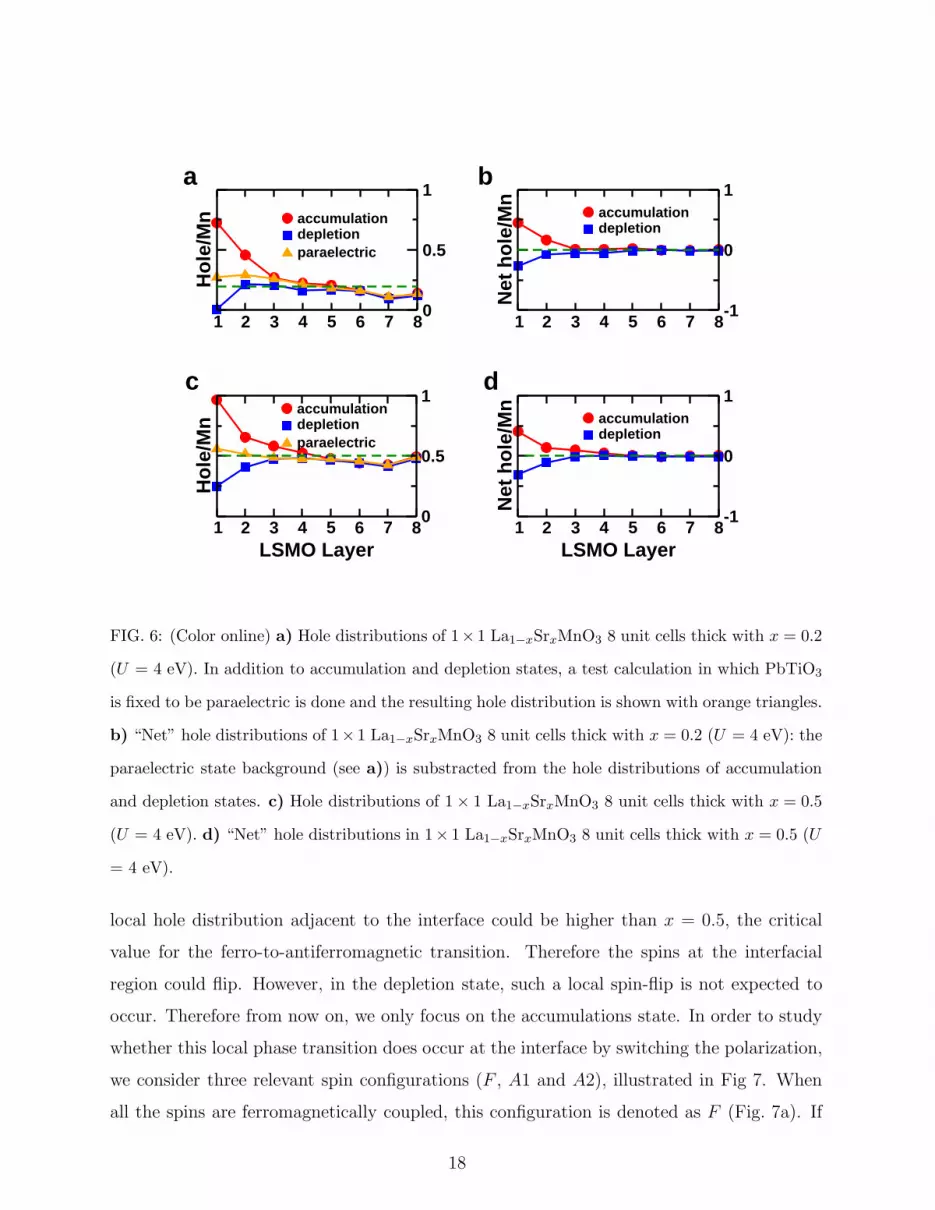
In order to get a spatial distribution of holes that is well converged with the manganite
thickness, we run a calculation with 8 unit cells of 1 × 1 La1−xSrxMnO3 . This calculation
is performed with LSDA+U (U=4 eV). The results are shown in Fig. 6. From Fig. 6a,
the screening length of the accumulation state is estimated to be 3 unit cells while the
screening length of depletion state seems to be only 1 unit cell. The asymmetry is due
to the fact that there are two factors affecting the hole distribution. One is the induced
screening charge and the other is the presence of PbO/MnO2 interface itself. To demonstrate
the role of the interface, we perform a test calculation in which the PbTiO3 thin film is
forced to be paraelectric and find (see the orange triangle symbols in Fig. 6a) that the
resulting hole distribution is not uniform nor equal to the nominial doping (x = 0.2) at
the interface. This non-uniform hole distribution can be considered as a background, owing
to the chemistry of the PbO/MnO2 interface. If we substract the hole distributions of
accumulation and depletion states from this background, we can see that the “net” hole
distributions of accumulation and depletion states now become more symmetric, with the
screening length of depletion state a little larger than that of accumulation state (Fig. 6b).
This is consistent with the Thomas-Fermi picture that depletion states have less carriers
(holes) and therefore a larger screening length. To further verify this Thomas-Fermi picture,
we perform the same calculation with a layer nominal hole doping x = 0.5 and find very
similar results (see Fig. 6c and d).
C. Magnetization modulation
In this section, we study in detail whether the charge modulation can induce a spin
modified configuration in the ground state. This means that the change of the magnetization
is not simply proportional to that of the charge density (i.e. simple filling/emptying of Mn
orbitals with fixed spin polarization) but involves a more dramatic change of magnetic
structure at the interface. The mechanism is as follows: in the accumulation state, the
17
a b
1 2 3 4 5 6 7 80
0.5
1H
ole/
Mn accumulation
depletionparaelectric
1 2 3 4 5 6 7 8-1
0
1
Net
hol
e/M
n accumulationdepletion
1 2 3 4 5 6 7 8LSMO Layer
0
0.5
1
Hol
e/M
n
accumulationdepletionparaelectric
1 2 3 4 5 6 7 8LSMO Layer
-1
0
1
Net
hol
e/M
n
c daccumulationdepletion
FIG. 6: (Color online) a) Hole distributions of 1× 1 La1−xSrxMnO3 8 unit cells thick with x = 0.2
(U = 4 eV). In addition to accumulation and depletion states, a test calculation in which PbTiO3
is fixed to be paraelectric is done and the resulting hole distribution is shown with orange triangles.
b) “Net” hole distributions of 1× 1 La1−xSrxMnO3 8 unit cells thick with x = 0.2 (U = 4 eV): the
paraelectric state background (see a)) is substracted from the hole distributions of accumulation
and depletion states. c) Hole distributions of 1× 1 La1−xSrxMnO3 8 unit cells thick with x = 0.5
(U = 4 eV). d) “Net” hole distributions in 1× 1 La1−xSrxMnO3 8 unit cells thick with x = 0.5 (U
= 4 eV).
local hole distribution adjacent to the interface could be higher than x = 0.5, the critical
value for the ferro-to-antiferromagnetic transition. Therefore the spins at the interfacial
region could flip. However, in the depletion state, such a local spin-flip is not expected to
occur. Therefore from now on, we only focus on the accumulations state. In order to study
whether this local phase transition does occur at the interface by switching the polarization,
we consider three relevant spin configurations (F , A1 and A2), illustrated in Fig 7. When
all the spins are ferromagnetically coupled, this configuration is denoted as F (Fig. 7a). If
18

FIG. 7: (Color online) Illustration of different magnetic structures. a) Ferromagnetic configuration,
denoted by F . b) Spin flips in the first unit cell, denoted by A1. c) Spin flips in the second unit
cell, denoted by A2.
the spin is flipped in the first unit cell of manganite from the interface, this configuration is
denoted by A1 (Fig. 7b). Finally, if the spin is flipped in the second unit cell of manganite,
then we denote it by A2 (Fig. 7c). We address three important and related questions below:
i) whether the ground-state magnetic structure depends on U? ii) given a reasonable U ,
whether the manganite nominal doping x could change the final magnetic structure? iii)
how the structural distortions at the interface may affect the magnetic structures?
1. Hubbard U dependence
We obtain the total energies of these three spin configurations with a range of Hubbard
U and collect all the results in Fig. 8. We use the following definitions of energy differences:
∆E1 = E(A1)−E(F ) (2)
∆E2 = E(A2)−E(F ) (3)
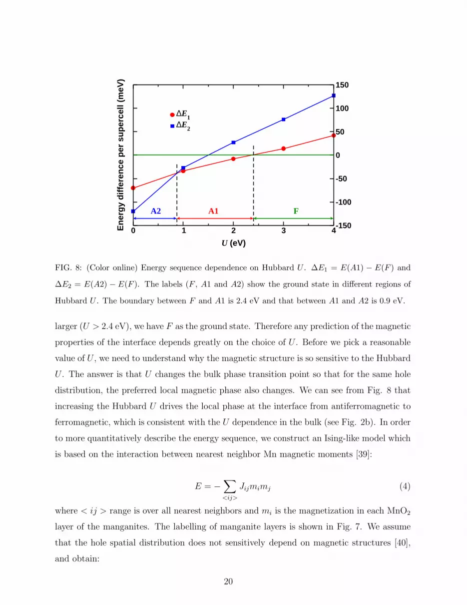
From Fig. 8 we can see that the magnetic structure of the ground state evolves with Hubbard
U . When U is small (U < 0.9 eV), the ground state has the magnetic structure of A2. With
U increasing (0.9 eV < U < 2.4 eV), the ground state evolves into A1. When U gets even
19
0 1 2 3 4
U (eV)
-150
-100
-50
0
50
100
150
Ene
rgy
diffe
renc
e pe
r su
perc
ell (
meV
)
A2 A1 F
∆E1∆E2
FIG. 8: (Color online) Energy sequence dependence on Hubbard U . ∆E1 = E(A1) − E(F ) and
∆E2 = E(A2) − E(F ). The labels (F , A1 and A2) show the ground state in different regions of
Hubbard U . The boundary between F and A1 is 2.4 eV and that between A1 and A2 is 0.9 eV.
larger (U > 2.4 eV), we have F as the ground state. Therefore any prediction of the magnetic
properties of the interface depends greatly on the choice of U . Before we pick a reasonable
value of U , we need to understand why the magnetic structure is so sensitive to the Hubbard
U . The answer is that U changes the bulk phase transition point so that for the same hole
distribution, the preferred local magnetic phase also changes. We can see from Fig. 8 that
increasing the Hubbard U drives the local phase at the interface from antiferromagnetic to
ferromagnetic, which is consistent with the U dependence in the bulk (see Fig. 2b). In order
to more quantitatively describe the energy sequence, we construct an Ising-like model which
is based on the interaction between nearest neighbor Mn magnetic moments [39]:
E = −∑
<ij>
Jijmimj (4)
where < ij > range is over all nearest neighbors and mi is the magnetization in each MnO2
layer of the manganites. The labelling of manganite layers is shown in Fig. 7. We assume
that the hole spatial distribution does not sensitively depend on magnetic structures [40],
and obtain:
20

∆E1 = 2J12|m1m2| (5)
∆E2 = 2J12|m1m2|+ 2J23|m2m3| (6)
In order to get an energy sequence, we need to know the signs of J12 and J23. From the
bulk calculations, at a given hole doping x and assuming half-metallicity, the magnetization
is related to the hole doping x by m = (4 − x)µB where µB is the Bohr magneton. The
exchange coupling J can be extracted out by:
J =E(A)− E(F )
2m2(7)
where the energy difference ∆E = E(A) − E(F ) is from the bulk calculations, shown in
Fig. 2. J changes sign at the transition point. From Eq. (7), J is positive for ferromagnetic
phase and negative for A-type antiferromagnetic phase. At the interface, however, the hole
spatial distribution is not uniform (see Fig. 6). We assume that the interface coupling Jij
is that of bulk La1−xSrxMnO3 but for a doping value that is the average of the neighboring
layers i and j:
Jij ≃ Jbulk
(
xi + xj
2
)
(8)
We need a final good approximation, which is verified in Fig. 5, that the hole distribution
does not sensitively depend on Hubbard U . Based on Eq. (5-8), we start with a large Hub-
bard U . Since large U favors ferromagnetism (see Fig. 2b), the bulk phase is ferromagnetic
and both J12 and J23 are positive. Thus 0 < ∆E1 < ∆E2 and we have the following energy
sequence: F < A1 < A2. We denote this by case 1. With a decreasing U , the transition
point is moved to smaller hole doping region. Noting that the hole distribution monoton-
ically decays from the interface (see Fig. 6), we always have (x1 + x2)/2 > (x2 + x3)/2.
Hence J12 changes sign earlier than J23 as U decreases. If U is in such a range that J12 just
becomes negative but J23 > 0, we have ∆E1 < 0 and ∆E2 > 0. The energy sequence is now
A1 < F < A2, which is denoted by case 2. As U further decreases, so that J12 becomes very
negative and J23 remains positive but J12|m1|+J23|m3| < 0, then we have ∆E1 < ∆E2 < 0.
The energy sequence becomes A1 < A2 < F . This is case 3. With U further decreasing, the
bulk phase becomes always antiferromagnetic, both J12 and J23 become negative, and we
21

TABLE IV: The energy sequence predicted from the simple model and the comparison with the
DFT calculations with different Hubbard U .
model DFT
case energy sequence U (eV) ∆E1 (meV) ∆E2 (meV)
1 0 < ∆E1 < ∆E2 3 14 76
2 ∆E1 < 0 < ∆E2 2 -8 27
3 ∆E1 < ∆E2 < 0 1 -34 -27
4 ∆E2 < ∆E1 < 0 0 -70 -120
have ∆E2 < ∆E1 < 0. The final possible energy sequence is A2 < A1 < F , which is denoted
by case 4. These four energy sequences exhaust all the possibilities and are summarized in
Table IV. Now we compare the DFT results (see Fig. 8) to the energy sequence predicted
from the model (see Table IV). As the Hubbard U evolves from 0 to 4 eV, we find all four
cases. For example, U = 3 eV corresponds to F < A1 < A2; U = 2 eV to A1 < F < A2;
U = 1 eV to A1 < A2 < F and U = 0 eV to A2 < A1 < F . The exact boundaries of
Hubbard U for each energy sequence can be found in Fig. 8.
Since the Hubbard U changes the transition point and the magnetic structure of the
ground state of the PbTiO3/La1−xSrxMnO3 interface, we need to determine what is the
reasonable value of U . Following Ref. [12], we argue that because the magnetic struc-
tures sensitively depend on the transition point, we need to choose a range of U so that
the ferromagnetic-to-antiferromagnetic transition occurs around x ≃ 0.5. From bulk cal-
culations, we know that as 1 eV < U < 2 eV for Pnma La1−xSrxMnO3, this criterion is
satisfied. On the other hand, when U is in this range, the magnetic structure of the ground
state is always A1. Therefore by switching the PbTiO3 polarization, we do find a spin-
modified configuration in the DFT simulation, provided that our choice of U is reasonable.
This prediction is consistent with the recent experiment [13] which observes an anomously
large change in the magnetization as the polarization of ferroelectrics is switched and which
assigns this to a spin-flip on the Mn atom closest to the interface.
22

0.2 0.3 0.4 0.5
hole x
-150
-100
-50
0
Ene
rgy
diffe
renc
e pe
r su
perc
ell (
meV
)
A2A1
∆E1∆E2
FIG. 9: (Color online) Energy dependences of the interfacial magnetic states as a function of the
doping x of the La1−xSrxMnO3. ∆E1 = E(A1)−E(F ) and ∆E2 = E(A2)−E(F ). The boundary
between the phases is at xc ≈ 0.22 denoted by the vertical dashed line. A1 is stable to the left and
A2 to the right of the boundary. The results are based on LSDA+U with U = 1 eV.
2. Hole dependence
The ground-state magnetic structure we found above (A1 configuration) is consistent
with the experimental conjecture, but it is different from the A2 configuration found using
DFT+GGA for the similar multiferroelectric structure BaTiO3/La1xBaxMnO3 with x =
0.5 [12]. We find that the reason for the differing ground state magnetic structure is due to
the doping x dependence of the system. Specifically, for U = 1 eV, we calculate the energies
of the A1 and A2 interfacial states versus doping x and present the results in Fig. 9.
When the nominal doping x is near the bulk magnetic transition point x = 0.5, the Fig. 9
shows that the ground state should be A2 which is consistent with Ref. [12]. However,
the actual experimental doping x = 0.2 is far below x = 0.5, the ground state should be
A1. We calculate the phase boundary between A1 and A2 to be xc ≈ 0.22 for U = 1
eV. This transition from A1 to A2 is easily understood in the framework of our Ising-like
model. Each pair of neighboring Mn magnetic moments could be either ferromagnetically or
23
antiferromagnetically coupled depending on the number of holes on the pair of Mn atoms.
When the doping x is low, the ferroelectric modulation of the hole density must drop to a
low value within a few unit cells from the interface (see Fig. 6) and thus only the first two
moments (m1, m2) will be paired antiferromagnetically, which leads to A1. However, when
the doping x is high, the larger values of the hole density means that both the (m1, m2) and
(m2, m3) pairs couple antiferromagnetically, which leads to A2. As a final remark, we note
that our Ising-like model predicts that the transition doping xc between A1 and A2 should
depend on Hubbard U : since increasing U favors ferromagnetism, larger U will increase xc
(i.e, require more holes for antiferromagnetism).
3. Structural distortion dependence
Due to the presence of ferroelectric polarization, significant distortions that deviate from
bulk manganites are observed in the relaxed ground state structures. Concerning each
oxygen octahedron that encloses Mn atoms, we calculate c/a ratio and rumplings δ/a in
each MnO2 layer, where c is the distance between the two apical oxygen atoms along the
z direction, δ is the vertical displacement between Mn and O, and a is the lattice constant
of SrTiO3 substrate. The results are summarized in Table V. Since the spin-flipped process
occurs at the interface in the accumulation state, we only show c/a ratio and δ/a of the
first and second manganite layers from the interface, and from now on the discussion is
constrained to the accumulation state. From Table V, we can see that in the accumulation
state, there are significant polar distortions at the interface (δ/a is as large as 6%). It was
shown in Ref. [12] that the spin-flipped process is mainly of electronic origin rather than
due to the polar distortions at the interface. In this section, we use detailed comparisons
to show that though the spin-modified configuration is due to electronic reconstructions,
polar distortions need to be taken into account in order to make a quantitative (instead of
qualitative) link between the interface phase and bulk phases.
Now we look at the Ising-like model Eq. (5-8) more closely. The model is based on the
assumption that the local magnetic structure can be predicted from bulk manganites of the
same hole doping. In Table VI, we list the energy difference between F and A1 interfacial
configurations from the interface calculations, defined by
24

TABLE V: The c/a ratio of each oxygen octahedron that encloses Mn atoms and rumplings δ/a
of each MnO2 layer for both accumulation and depletion states. c is the distance between the
two apical oxygen atoms along the z direction. δ is the rumplings of MnO2 layer, and a is the
lattice constant of SrTiO3 substrate. Layer1 and layer2 refer to the first and second unit cell of
manganites from the interface.
accumulation state depletion state
layer1 layer2 layer1 layer2
c/a 0.97 0.94 c/a 1.05 0.98
δ/a 0.06 0.02 δ/a 0.01 0.001
∆EI = E(A1)− E(F ) (9)
where E(F ) and E(A1) are the total energies of F and A1 configurations, respectively.
We also calculate the average hole density between the first and second layers, i.e. x =
(x1 + x2)/2. Next, we list the bulk energy difference ∆EB, defined as
∆EB =1
2(EB(A)−EB(F )) (10)
where EB(F ) and EB(A) are the total energies of SrTiO3-strained La1−xSrxMnO3 with
ferromagnetic and A-type antiferromagnetic ordering, respectively. The factor 1
2is included
because in the bulk form wherever a Mn atom flips its spin, there are two Mn-Mn bonds
involved owing to periodic boundary conditions, whereas at the interface a Mn spin flip only
involves one Mn-Mn bond. Hence, we need a factor 1
2so that both ∆EI and ∆EB describe
the energy difference per Mn-Mn bond. The nominal hole doping x is chosen as the same
as x from the supercell calculations. Table VI shows that although the trend versus U is
the same in both supercell and bulk calculations, the magnitudes of ∆E do not agree at all.
There must be something at the interface which is absent in bulk phase and significantly
affects the energy difference between antiferro- and ferromagnetism.
We find that, due to the presence of ferroelectric PbTiO3, strong polar distortions are
induced at the interface layer of MnO2 in the accumulation state (Table V), as is illus-
25
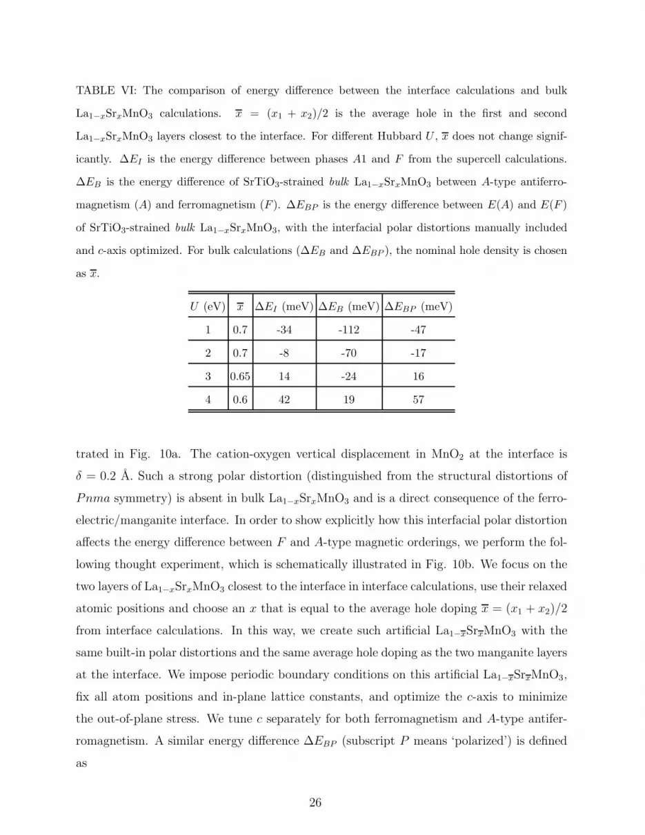
TABLE VI: The comparison of energy difference between the interface calculations and bulk
La1−xSrxMnO3 calculations. x = (x1 + x2)/2 is the average hole in the first and second
La1−xSrxMnO3 layers closest to the interface. For different Hubbard U , x does not change signif-
icantly. ∆EI is the energy difference between phases A1 and F from the supercell calculations.
∆EB is the energy difference of SrTiO3-strained bulk La1−xSrxMnO3 between A-type antiferro-
magnetism (A) and ferromagnetism (F ). ∆EBP is the energy difference between E(A) and E(F )
of SrTiO3-strained bulk La1−xSrxMnO3, with the interfacial polar distortions manually included
and c-axis optimized. For bulk calculations (∆EB and ∆EBP ), the nominal hole density is chosen
as x.
U (eV) x ∆EI (meV) ∆EB (meV) ∆EBP (meV)
1 0.7 -34 -112 -47
2 0.7 -8 -70 -17
3 0.65 14 -24 16
4 0.6 42 19 57
trated in Fig. 10a. The cation-oxygen vertical displacement in MnO2 at the interface is
δ = 0.2 A. Such a strong polar distortion (distinguished from the structural distortions of
Pnma symmetry) is absent in bulk La1−xSrxMnO3 and is a direct consequence of the ferro-
electric/manganite interface. In order to show explicitly how this interfacial polar distortion
affects the energy difference between F and A-type magnetic orderings, we perform the fol-
lowing thought experiment, which is schematically illustrated in Fig. 10b. We focus on the
two layers of La1−xSrxMnO3 closest to the interface in interface calculations, use their relaxed
atomic positions and choose an x that is equal to the average hole doping x = (x1 + x2)/2
from interface calculations. In this way, we create such artificial La1−xSrxMnO3 with the
same built-in polar distortions and the same average hole doping as the two manganite layers
at the interface. We impose periodic boundary conditions on this artificial La1−xSrxMnO3,
fix all atom positions and in-plane lattice constants, and optimize the c-axis to minimize
the out-of-plane stress. We tune c separately for both ferromagnetism and A-type antifer-
romagnetism. A similar energy difference ∆EBP (subscript P means ‘polarized’) is defined
as
26
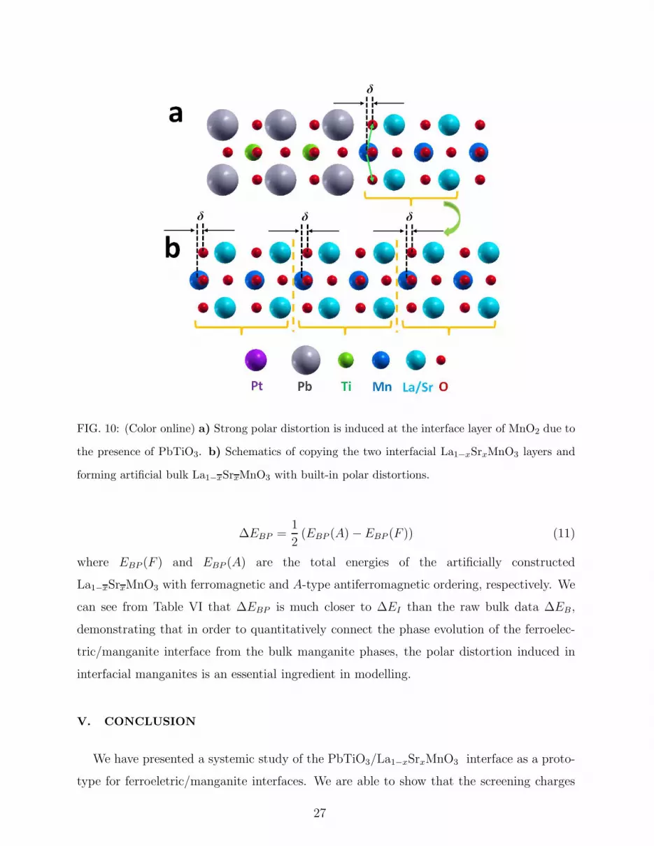
FIG. 10: (Color online) a) Strong polar distortion is induced at the interface layer of MnO2 due to
the presence of PbTiO3. b) Schematics of copying the two interfacial La1−xSrxMnO3 layers and
forming artificial bulk La1−xSrxMnO3 with built-in polar distortions.
∆EBP =1
2(EBP (A)−EBP (F )) (11)
where EBP (F ) and EBP (A) are the total energies of the artificially constructed
La1−xSrxMnO3 with ferromagnetic and A-type antiferromagnetic ordering, respectively. We
can see from Table VI that ∆EBP is much closer to ∆EI than the raw bulk data ∆EB,
demonstrating that in order to quantitatively connect the phase evolution of the ferroelec-
tric/manganite interface from the bulk manganite phases, the polar distortion induced in
interfacial manganites is an essential ingredient in modelling.
V. CONCLUSION
We have presented a systemic study of the PbTiO3/La1−xSrxMnO3 interface as a proto-
type for ferroeletric/manganite interfaces. We are able to show that the screening charges
27
produced in the manganite in response to the ferroelectric surface charge are sufficient to
change the magnetic state of the interfacial manganite from ferromagnetic to antiferromag-
netic, in agreement with experimental observations and interpretations. In the process, we
have developed a method to accurately count the layer-by-layer hole distribution in the
manganite thin film which allows us to perform quantitative analysis of the system. For
example, it allows us to create a simple Ising-like model of the interfacial magnetism that
uses bulk parameters to reproduce the computed behaviors.
One of main theoretical findings is that the ground-state magnetic state depends sen-
sitively on the value of U chosen in the LSDA+U computation. We show that different
reasonable-seeming approaches to determining U , and in particular some that are ab initio
and deliver a U value appropriate to LSDA+U self-consistently, yield significantly different
U values. Not all the values do well when compared to experiment. By asking that the
LSDA+U calculation should correctly reproduce the critical hole doping density separating
the ferromagnetic and antiferromagnetic phases, we are able to find a narrow range of U
values that also produce a straightforward interfacial magnetic ground-state structure (the
A1 configuration) whereby the manganite layer with the highest doping has the strongest
magnetic response. Clearly, our conclusions on the magnetic ground-state are not ab initio
as they involve significant experimental input. In our opinion, the unsatisfactory situa-
tion vis a vis choosing the U value is due to the limitations of the single-particle DFT+U
method itself when applied to a complex and strongly correlated electronic system such as
manganites: the theory is not accurate enough for the material, so some level of empiricism
is unfortunately necessary.
Acknowledgments
We are grateful to useful discussions with Carlos A. F. Vaz, Jason Hoffman, Yaron Segal,
Fred J. Walker, Alexie M. Kolpak and Charles H. Ahn. This work was supported primarily
by the National Science Foundation under Contracts No. MRSEC DMR 0520495 and DMR
1119826 and in part by the facilities and staff of the Yale University Faculty of Arts and
Sciences High Performance Computing Center and by the National Science Foundation
under grant #CNS 08-21132 that partially funded acquisition of the facilities. Bulldog
parallel clusters of the Yale High Performance Computing center and TeraGrid provided
28

computational resources.
Appendix A: Tests of the virtual crystal approximation
We treat the A-site La1−xSrx alloying in La1−xSrxMnO3 with the virtual crystal approx-
imation [21, 22]. This approximation involves replacing the two elements by a fictitious one
whose electron number is (1−x)NLa+xNSr, where NLa and NSr are the number of electrons
of the La and Sr pseudo atoms, respectively. We stress that i) since the magnetic properties
originate from Mn d-electrons and A-site atoms serve to donate electrons, we expect that
the virtual crystal approximation is reasonable to describe the magnetic phase transition
of manganites in the random distribution; ii) since the chemical properties mainly depend
on the valence electrons, the approximation we make here is expected to be also good for
Ca and Ba, and iii) our choice of pseudo potential and valence electrons shown in Table I
ensures a very smooth interpolation between La and Sr as their pseudo valence electrons and
nuclear pseudo charges only differ by one elementary charge. We perform simple tests of 1:1
Sr-La alloying (i.e. 50% alloying) in a c(2 × 2) × 2 unit cell and the results are compared
to the x = 0.5 virtual crystal approximation as shown in Table VII. We can see that virtual
crystal approximation quantitatively reproduces the lattice constants and the energy differ-
ences between various magnetic orderings when compared to the calculation with “real” La
and Sr atoms. The accuracy of magnetic energy differences is consistent with earlier work
[23].
Appendix B: The effects of SrTiO3 substrate
Inclusion of SrTiO3 substrate in the simulation of PbTiO3/La1−xSrxMnO3 heterostruc-
tures is computationally intensive. In this section, we test the effects of SrTiO3 substrate
on structrual and magnetic properties on the PbTiO3/La1−xSrxMnO3 interface. We com-
pare two calculations: one with three unit cells of SrTiO3 and the other without SrTiO3.
La1−xSrxMnO3 is four unit cells thick with nominal doping x = 0.2. PbTiO3 thin film is
polarized so that both calculations are in the accumulation state. In terms of structural
properties, we focus on two important quantities. One is the c/a ratio of each oxygen oc-
tahedron that encloses Mn atoms. The other is the rumpling δ of each MnO2 layer. The
29

TABLE VII: Comparison between the virtual crystal approximation and supercell calculations.
The nominal doping x is 0.5 in the virtual crystal approximation. A c(2 × 2) × 2 supercell is
employed with La and Sr atoms forming a checker-board pattern (every nearest neighbor of Sr is
La and vice versa). The lattice constants reported are those for A-type antiferromagnetic ordering.
∆E is the energy difference between ferromagnetic ordering and A-type antiferromagnetic ordering
per Mn atom, defined by Eq. (1). A range of Hubbard U (0 ≤ U ≤ 2 eV) are tested.
Virtual crystal approximation c(2 × 2)× 2 supercell
U (eV) a (A) b (A) c (A) ∆E (meV) a (A) b (A) c (A) ∆E (meV)
F A F A F A F A F A F A
0 5.345 5.363 7.561 7.385 5.386 5.408 -34 5.327 5.366 7.482 7.372 5.381 5.411 -37
1 5.385 5.376 7.612 7.411 5.430 5.433 -10 5.355 5.380 7.513 7.398 5.400 5.439 -11
2 5.401 5.380 7.623 7.422 5.434 5.452 7 5.365 5.387 7.520 7.411 5.410 5.452 6
results are shown in Fig. 11A. Layer 1 is the interface. Layer 4 is the artificial surface when
SrTiO3 is absent. The solid symbols are with SrTiO3 and the open symbols are without
SrTiO3. We can see that the structural properties with or without SrTiO3 substrate quickly
converge as the interface is approached. At Layer 1, the difference is negligible. In terms of
magnetic properties, we calculate the d-orbital magnetic moment of each Mn atom, using
the Lowdin orbitals approach [16]. Fig. 11B shows the comparison between with SrTiO3
substrate (solid symbols) and without SrTiO3 substrate (open symbols). Similar to struc-
tural properties, the effects of SrTiO3 substrate on magnetic properties are generally very
small and diminish at the interface. Therefore we do not include SrTiO3 substrate in our
simulation, not only to reduce the computation burden but also to introduce an artificial
surface so that we can apply a counting method (see Appendix C) to accurately calculate
hole distribution in La1−xSrxMnO3.
30

FIG. 11: (Color online) The effects of SrTiO3 substrate on structural and magnetic properties at
the PbTiO3/La1−xSrxMnO3 interface. Layer1 is the interfacial layer of MnO2. The solid symbols
correspond to the data with SrTiO3 substrate. The open symbols correspond to the data without
SrTiO3 substrate. A) rumplings of each MnO2 layer and c/a ratio of each oxygen octahedron that
encloses Mn atoms. B) d-orbital magnetic moment of each Mn atom, calculated by using Lowdin
orbitals.
Appendix C: The method for counting holes
A widely used approach for calculating the number of holes and the magnetization of Mn
atoms is to use Lowdin orbitals [16]. However, a more direct method is to use the electron
density itself. The difficulty lies in that the boundary between each manganite layer is not
well-defined in the thin film of La1−xSrxMnO3. We develop a method to self-consistently set
the boundary between each manganite layer, provided that the manganite is half-metallic.
For a half-metallic manganite, there are no states at the Fermi level in the minority spin
channel, so that there must be a definite integer number of electrons Nc filled in the minority
spin channel. Nc depends on the details of pseudopotentials. For our pseudo atoms (see
Table I), for doping level x, we have La3+: 5s25p65d06s0, Sr2+: 4s24p65s0, O2−: 2s22p6 and
due to charge conservation, Mn ion is nominally +(3 + x) with an electron configuration
3s23p63d4−x4s0. For one unit cell of La1−xSrxMnO3, since spin polarization only comes from
the electrons on Mn d-orbitals, we can sum all the other electrons that are formally spin
unpolarized: 8× (1−x)+ 8×x+8× 3+8 = 40. The four terms are from La3+, Sr2+, three
O2− and the Mn ion without d-electrons. Hence Nc = 40/2 = 20, which is independent of
31

FIG. 12: (Color online) Illustration of how to count the charge in each layer of La1−xSrxMnO3. The
spin polarized part is La1−xSrxMnO3. The green dashed lines highlight the computed boundaries
of each layer.
hole doping. Now we start from the vacuum (see Fig. 12) where there is no charge. We
integrate the minority spin channel moving into the film until the integral is equal to 20.
Then this position determines the boundary of the first layer. Next we restart the integral
from this boundary until it reaches 20 again. This determines the boundary of the second
layer. Repeating the procedure yields the boundaries of each manganite layer. Once the
boundaries are determined, we integrate the charge density of both majority and minority
spins in each layer and thus layer-resolved holes and magntization follow straightforwardly.
We comment that in DFT calculations, as long as the Hubbard U is larger than a critical
value Uc, the manganites become half-metallic in the ferromagnetic phase. For SrTiO3-
strained Pnma La1−xSrxMnO3, we find Uc ≃ 1 eV. Therefore, for the useful and reasonable
range of U , our method is valid.
32

0 0.2 0.4 0.6 0.8 1
Hole doping x
-300
-200
-100
0
100
200
300
∆ E
/Mn
(meV
)
F A C G
A-typeC-typeG-type
FIG. 13: (Color online) The complete magnetic phase diagram of La1−xSrxMnO3 (4 formula,
20 atoms). The calculation is based on LSDA+U with U = 1 eV. ∆E is the energy difference
between ferromagnetism and various types of anti-ferromagnetism. The labels F , A, C and G
refer to ferromagnetism, A-type, C-type and G-type antiferromagnetism, respectively. Each label
highlights the ground state magnetic structure of the given hole doping region.
Appendix D: The phase diagram of manganites from LSDA+U
In this section, we provide the complete magnetic phase diagram of La1−xSrxMnO3
in Fig. 13 based on LSDA+U with U = 1 eV. In the high doping region (x > 0.4),
LSDA+U does reproduce the experimentally observed sequence of different magnetic ground
states [23]: FM → A−AFM → C −AFM → G−AFM as the hole doping x increases. Our
result is consistent with previous calculations [12].
Appendix E: Test of band alignment and possible artificial charge spillage
Due to the well known underestimation of band gaps in DFT calculations, band align-
ment errors and possible artificial charge spillage into the conduction bands of on material
at an interface may occur. These errors can lead to unrealistic ground states when sim-
ulating the interface between ferroelectrics and metals [37]. We check our calculations of
33

Ti-dO-p
Layer1 (IF)
Layer2
Layer3
Layer4
Layer1 (IF)
Layer2
Layer3
Layer4
ba
Ti-dO-p
PD
OS
(ar
bitr
ary
unit)
7 8 9 10 11 12 13E (eV)
PD
OS
(ar
bitr
ary
unit)
7 8 9 10 11 12 13E (eV)
FIG. 14: (Color online) Atomic projected density of states (PDOS) of PbTiO3 in the
PbTiO3/La1−xSrxMO3/Pt heterostructures. a) The accumulation state. b) The depletion state.
The red curves are Ti-d projected states and the blue curves are O-p projected states. Layer1
refers to the interface between PbTiO3 and La1−xSrxMnO3 (the interface we are interested in) and
Layer4 is the interface between PbTiO3 and Pt. The green solid line is the Fermi level.
PbTiO3/La1−xSrxMO3/Pt interface and find that the Fermi level is in the band gap of
PbTiO3. A typical projected density of states (PDOS) of both the accumulation and de-
pletion states is illustrated in Fig. 14, where Layer1 refers to the interface between PbTiO3
and La1−xSrxMnO3 (the interface we are interested in) and Layer4 is the interface between
PbTiO3 and Pt. We can see that the interior of PbTiO3 remains insulating. We need to
point out that both terminations of PbTiO3 are PbO layers in our calculations, instead of
the pathological TiO2 termination which leads to a metallic ferroelectric ground state in
other similar systems [37].
34

[1] W. Eerenstein, N. D. Mathur, and J. F. Scott, Nature 442, 759 (2006).
[2] R. Ramesh and N. A. Spaldin, Nat. Mater. 6, 21 (2007).
[3] K. F. Wang, J. M. Liu, and Z. F. Ren, Adv. Phys. 58, 321 (2009).
[4] C. A. F. Vaz, J. Hoffman, C. H. Ahn, and R. Ramesh, Advanced Materials 22, 2900 (2010).
[5] I. Dzyaloshinskii, Soviet Phys. J. Expt. Theor. Phys. 10, 628629 (1960).
[6] G. Srinivasan, E. T. Rasmussen, J. Gallegos, R. Srinivasan, Y. I. Bokhan, and V. M. Laletin,
Phys. Rev. B 64, 214408 (2001).
[7] N. A. Spaldin and M. Fiebig, Science 309, 391 (2005).
[8] C.-G. Duan, S. S. Jaswal, and E. Y. Tsymbal, Phys. Rev. Lett. 97, 047201 (2006).
[9] K. Yamauchi, B. Sanyal, and S. Picozzi, Appl. Phys. Lett. 91, 062506 (2007).
[10] M. K. Niranjan, J. P. Velev, C.-G. Duan, S. S. Jaswal, and E. Y. Tsymbal, Phys. Rev. B 78,
104405 (2008).
[11] J. M. Rondinelli, M. Stengel, and N. A. Spaldin, Nat. Nanotech. 3, 46 (2008).
[12] J. D. Burton and E. Y. Tsymbal, Phys. Rev. B 80, 174406 (2009).
[13] C. A. F. Vaz, J. Hoffman, Y. Segal, J. W. Reiner, R. D. Grober, Z. Zhang, C. H. Ahn, and
F. J. Walker, Phys. Rev. Lett. 104, 127202 (2010).
[14] V. Garcia, S. Fusil, K. Bouzehouane, S. Enouz-Vedrenne, N. D. Mathur, A. Barthelemy, and
M. Bibes, Nature 460, 81 (2009).
[15] N. C. Bristowe, M. Stengel, P. B. Littlewood, J. M. Pruneda, and E. Artacho, Phys. Rev. B
85, 024106 (2012).
[16] P.-O. Lowdin, J. Chem. Phys. 18, 365 (1950).
[17] M. C. Payne, M. P. Teter, D. C. Allan, T. A. Arias, and J. D. Joannopoulos, Rev. Mod. Phys.
64, 1045 (1992).
[18] D. Vanderbilt, Phys. Rev. B 41, 7892 (1990).
[19] W. Kohn and L. J. Sham, Phys. Rev. 140, A1133 (1965).
[20] V. I. Anisimov, F. Aryasetiawan, and A. I. Lichtenstein, J. Phys.: Condens. Matter 9, 767
(1997).
[21] L. Nordheim, Ann. Phys. (Leipzig) 9, 607 (1931).
[22] L. Bellaiche and D. Vanderbilt, Phys. Rev. B 61, 7877 (2000).
35

[23] Z. Fang, I. V. Solovyev, and K. Terakura, Phys. Rev. Lett. 84, 3169 (2000).
[24] Y. Nohara, A. Yamasaki, S. Kobayashi, and T. Fujiwara, Phys. Rev. B 74, 064417 (2006).
[25] G. Trimarchi and N. Binggeli, Phys. Rev. B 71, 035101 (2005).
[26] C. Zener, Phys. Rev. 82, 403 (1951).
[27] Y. Tokura, Rep. Prog. Phys. 69, 797 (2006).
[28] H. A. Kramers, Physica 1, 182 (1934).
[29] A. Sadoc, B. Mercey, C. Simon, D. Grebille, W. Prellier, and M.-B. Lepetit, Phys. Rev. Lett.
104, 046804 (2010).
[30] I. V. Solovyev, Phys. Rev. B 69, 134403 (2004).
[31] I. Solovyev, N. Hamada, and K. Terakura, Phys. Rev. Lett. 76, 4825 (1996).
[32] P. W. Anderson and H. Hasegawa, Phys. Rev. 100, 675 (1955).
[33] T. Hashimoto, S. Ishibashi, and K. Terakura, Phys. Rev. B 82, 045124 (2010).
[34] M. Cococcioni and S. de Gironcoli, Phys. Rev. B 71, 035105 (2005).
[35] H. J. Kulik, M. Cococcioni, D. A. Scherlis, and N. Marzari, Phys. Rev. Lett. 97, 103001
(2006).
[36] R. D. King-Smith and D. Vanderbilt, Phys. Rev. B 47, 1651 (1993).
[37] M. Stengel, P. Aguado-Puente, N. A. Spaldin, and J. Junquera, Phys. Rev. B 83, 235112
(2011).
[38] See http://www.quantum-espresso.org
[39] The original Ising model with Hamiltonian of the form∑
ij JijSiSj can not be justified rigor-
ously from first principles here because our system is metallic and there are no isolated spins.
Instead, we use layer-resolved magnetization mi as a basis variable to create an effective model
for our system which has the form of an Ising Hamiltonian.
[40] We used a Lowdin orbital analysis and found that the change in the hole spatial distribution
between different magnetic structures is insignificant. However, just as we argued in the ap-
pendix, the Lowdin method itself is not highly accurate and can only be considered to provide
indirect evidence.
36