Feature Detection

Image features
• Global features – global properties of an image, including intensity
histogram, frequency domain descriptors, covariance matrix and high order statistics, etc.
• Local features – local regions with special properties, including edges,
corners, lines, curves, regions with special properties, etc
• Depending on applications, various features are useful. We will focus on edges and corners in this lecture
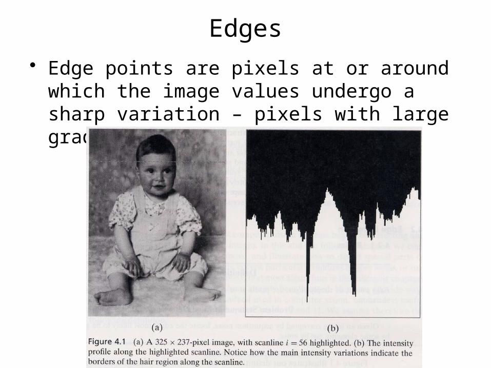
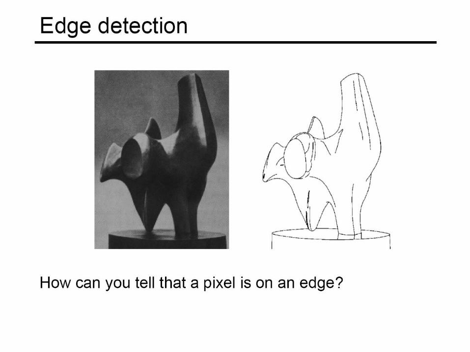
Edges
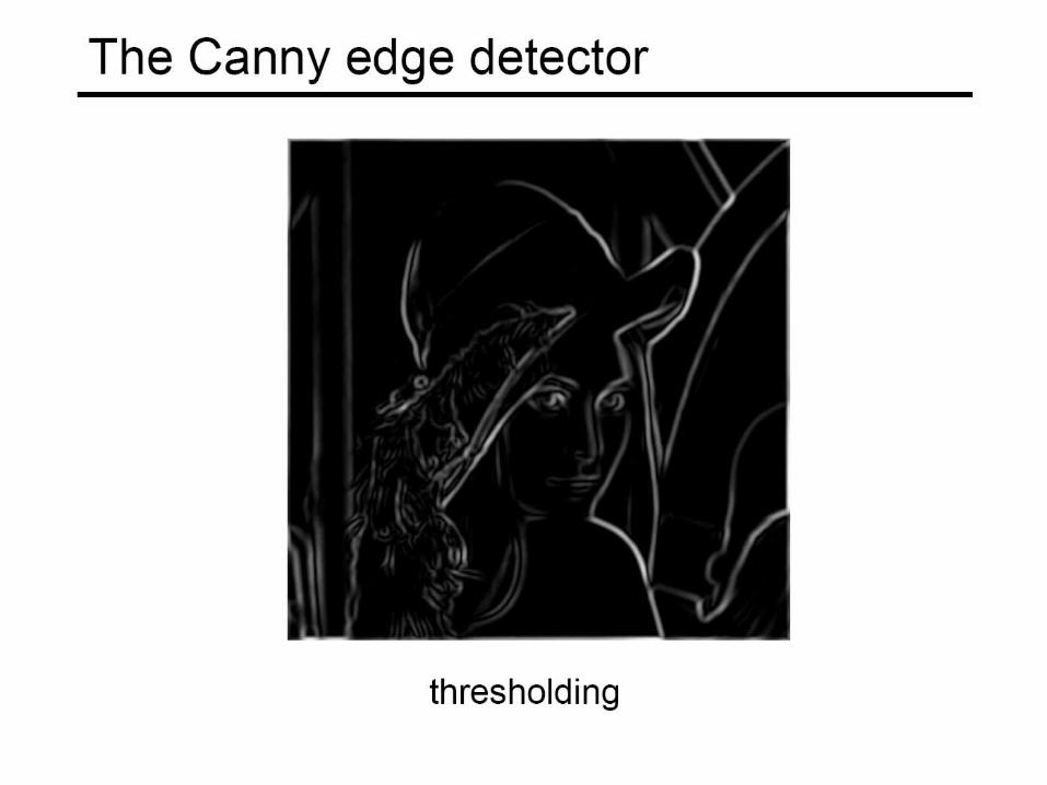
• Edge points are pixels at or around which the image values undergo a sharp variation – pixels with large gradient


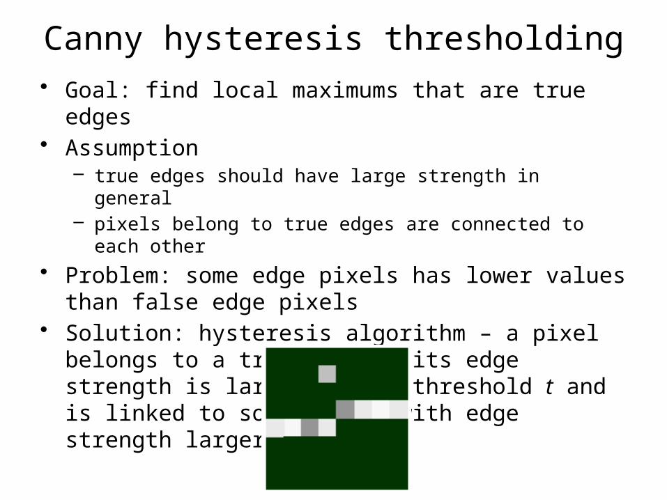
Canny hysteresis thresholding• Goal: find local maximums that are true edges• Assumption
– true edges should have large strength in general– pixels belong to true edges are connected to each other
• Problem: some edge pixels has lower values than false edge pixels
• Solution: hysteresis algorithm – a pixel belongs to a true edge if its edge strength is larger than a threshold t and is linked to some points with edge strength larger than t
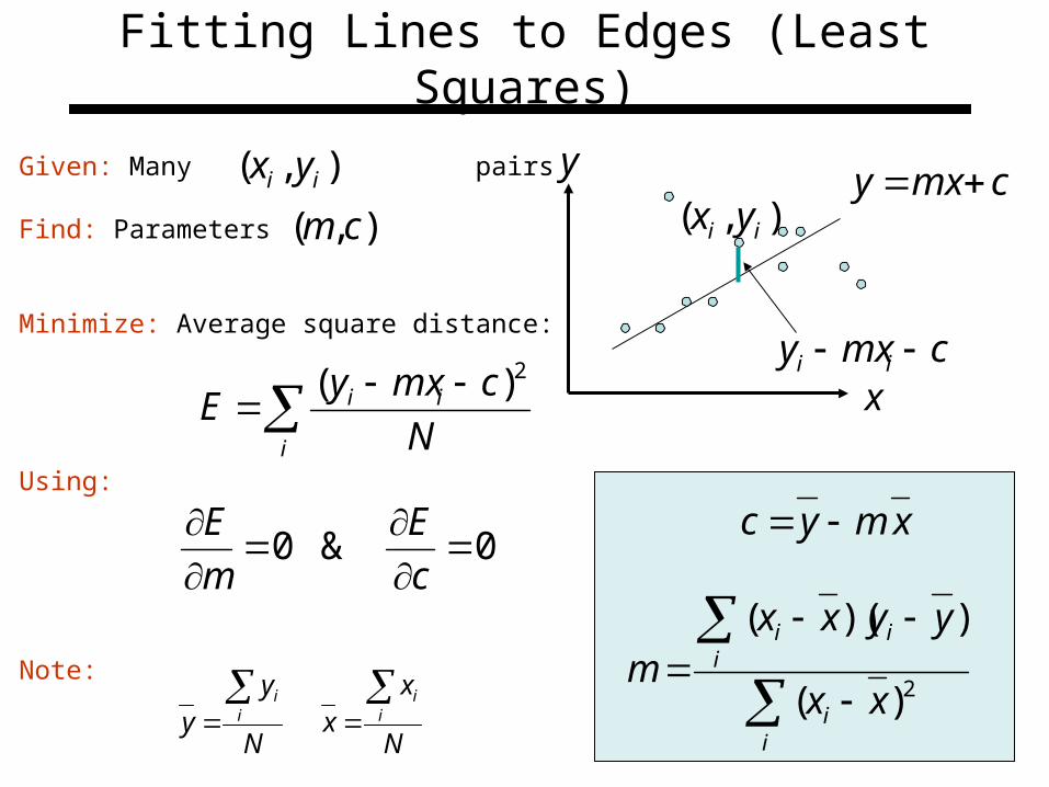
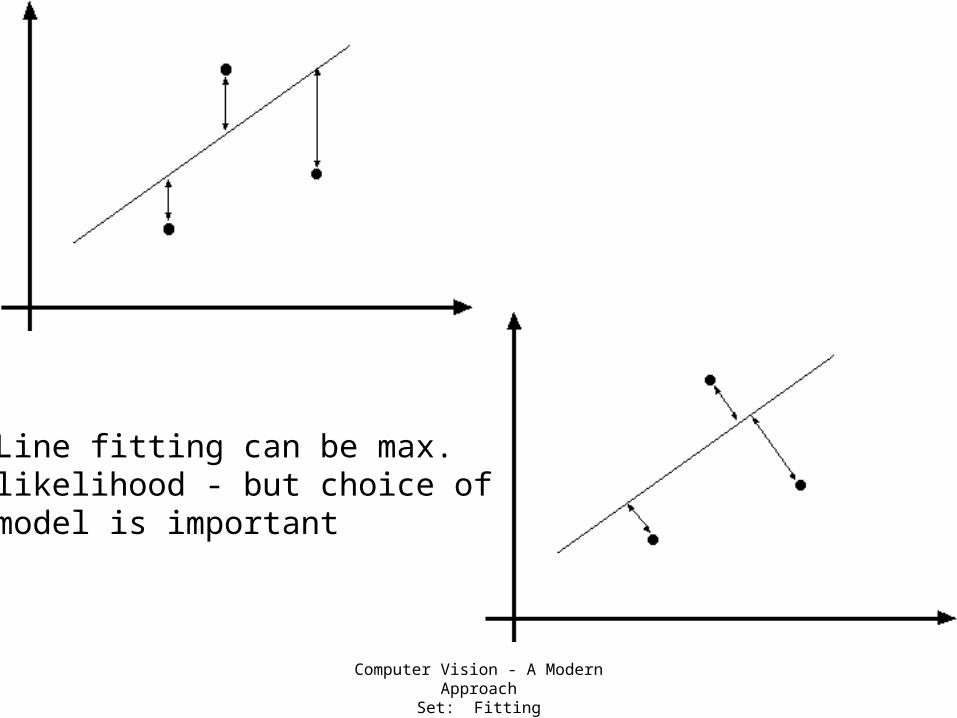
Fitting Lines to Edges (Least Squares)
cmxy
cmxy ii
),( ii yx
y
x
Given: Many pairs
Find: Parameters
Minimize: Average square distance:
Using:
Note:
),( ii yx
),( cm
i
ii
N
cmxyE
2)(
0&0
c
E
m
E xmyc
ii
iii
xx
yyxxm
2)(
))((
N
yy i
i
N
xx i
i

Problem with Parameterization
y
x
Line that minimizes E!!
Solution: Use a different parameterization
(same as the one we used in computing Minimum Moment of Inertia)
Note: Error E must be formulated carefully!
i
ii yxN
E 2)sincos(1
Computer Vision - A Modern ApproachSet: Fitting
Slides by D.A. Forsyth
Line fitting can be max.likelihood - but choice ofmodel is important
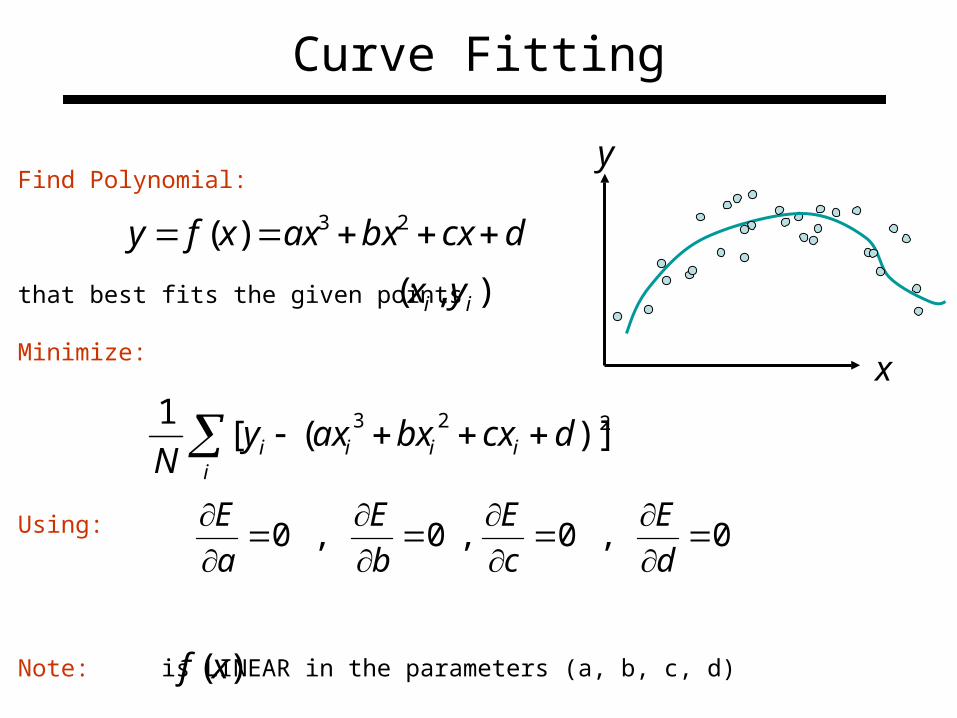
Curve Fitting
y
x
Find Polynomial:
that best fits the given points
Minimize:
Using:
Note: is LINEAR in the parameters (a, b, c, d)
),( ii yx
dcxbxaxxfy 23)(
i
iiii dcxbxaxyN
223 )]([1
0,0,0,0
d
E
c
E
b
E
a
E
)(xf

Line Grouping Problem
Slide credit: David Jacobs

This is difficult because of:
• Extraneous data: clutter or multiple models– We do not know what is part of the model?– Can we pull out models with a few parts from much
larger amounts of background clutter?
• Missing data: only some parts of model are present
• Noise
• Cost:– It is not feasible to check all combinations of features
by fitting a model to each possible subset

Hough Transform
• Elegant method for direct object recognition
• Edges need not be connected
• Complete object need not be visible
• Key Idea: Edges VOTE for the possible model
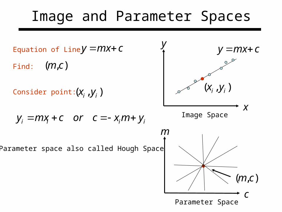
Image and Parameter Spaces
cmxy
),( ii yx
y
x
Equation of Line:
Find:
Consider point:
cmxy
),( cm
),( ii yx
iiii ymxcorcmxy m
c
),( cm
Image Space
Parameter Space
Parameter space also called Hough Space

Line Detection by Hough Transformy
x
),( cm
Parameter Space
1 1
1 1
1 1
2
1 1
1 1
1 1
),( cmA
Algorithm:
• Quantize Parameter Space
• Create Accumulator Array
• Set
• For each image edge increment:
• If lies on the line:
• Find local maxima in
),( cm
),( cmA
cmcmA ,0),(
),( ii yx
1),(),( cmAcmA
),( cm
),( cmAii ymxc

Better Parameterization
NOTE:
Large Accumulator
More memory and computations
Improvement:
Line equation:
Here
Given points find
m
sincos yx
max0
20
(Finite Accumulator Array Size)
),( ii yx ),(
),( ii yx
y
xImage Space
Hough Space
?
Hough Space Sinusoid
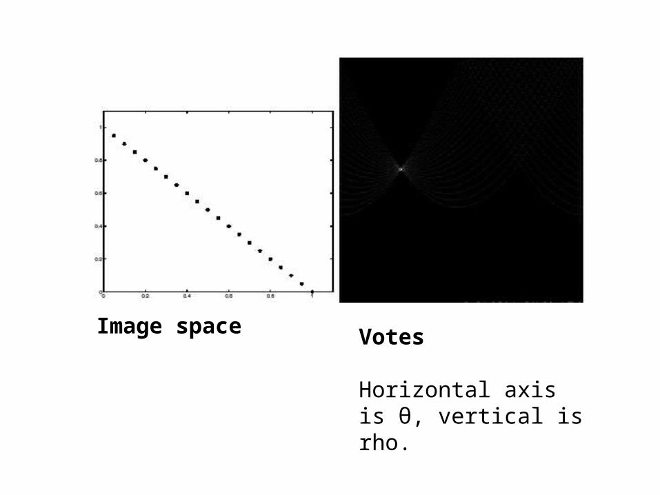
Image space Votes
Horizontal axis is θ, vertical is rho.

Image space
votes

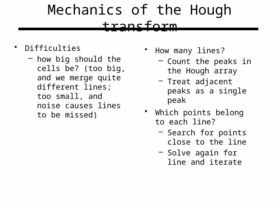
Mechanics of the Hough transform
• Difficulties– how big should the cells
be? (too big, and we merge quite different lines; too small, and noise causes lines to be missed)
• How many lines?– Count the peaks in the
Hough array– Treat adjacent peaks as
a single peak
• Which points belong to each line?– Search for points close to
the line– Solve again for line and
iterate

Fewer votes land in a single bin when noise increases.
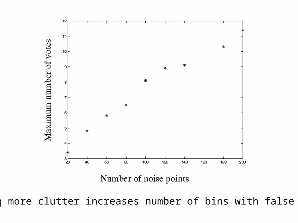
Adding more clutter increases number of bins with false peaks.
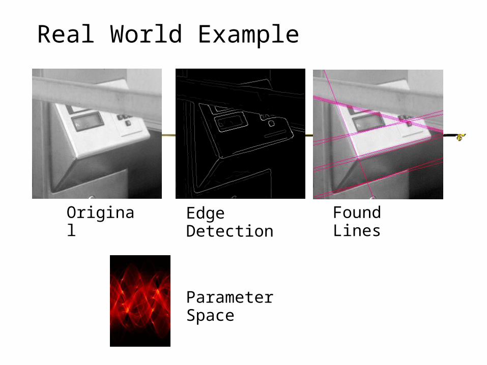
Real World Example
Original Edge Detection
Found Lines
Parameter Space

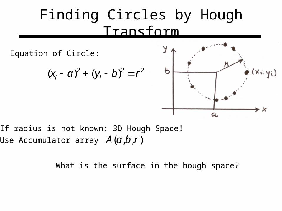
Finding Circles by Hough Transform
Equation of Circle:
222 )()( rbyax ii
If radius is known:
),( baAAccumulator Array
(2D Hough Space)
Finding Circles by Hough Transform
Equation of Circle:
222 )()( rbyax ii
If radius is not known: 3D Hough Space!
Use Accumulator array ),,( rbaA
What is the surface in the hough space?
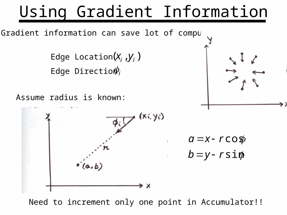
Using Gradient Information• Gradient information can save lot of computation:
Edge Location
Edge Direction
Need to increment only one point in Accumulator!!
i),( ii yx
Assume radius is known:
sin
cos
ryb
rxa
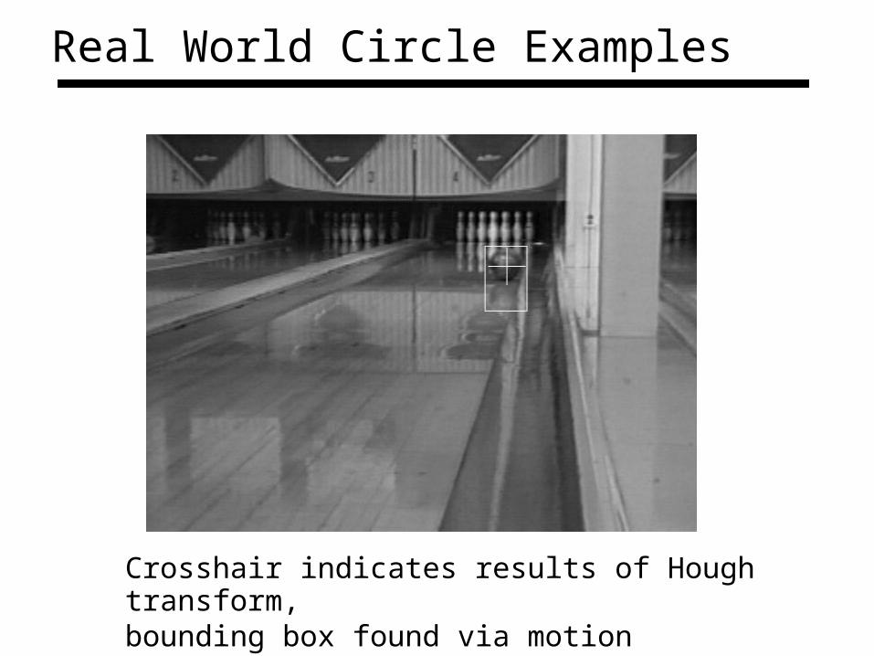
Real World Circle Examples
Crosshair indicates results of Hough transform,bounding box found via motion differencing.

Finding Coins
Original Edges (note noise)

Finding Coins (Continued)
Penny
Quarters

Finding Coins (Continued)
Coin finding sample images from: Vivek Kwatra
Note that because the quarters and penny are different sizes, a different Hough transform (with separate accumulators) was used for each circle size.

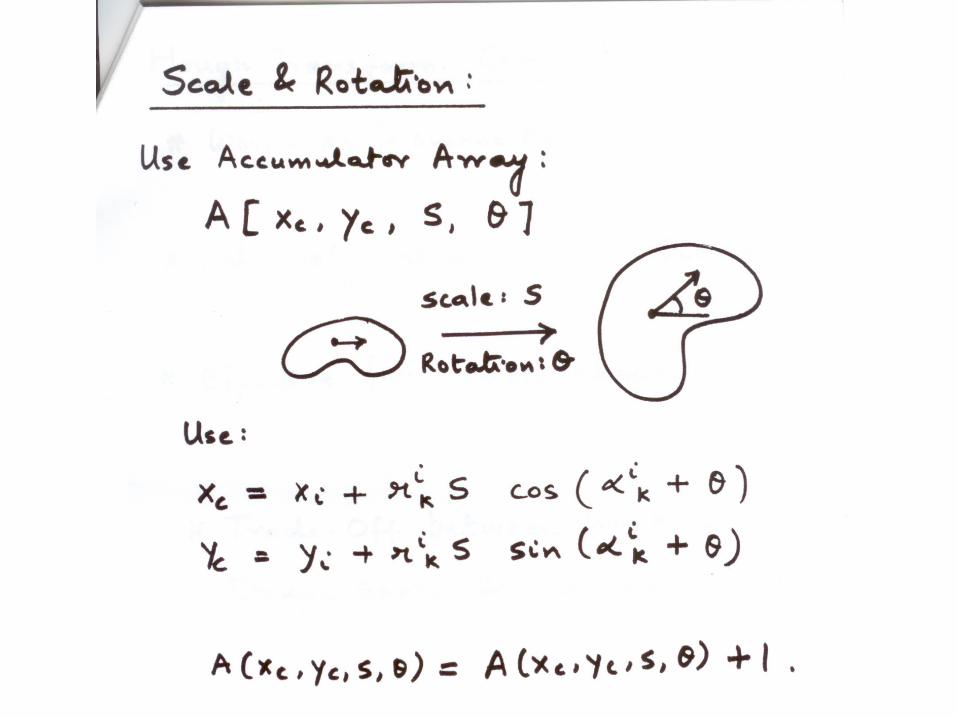
Generalized Hough Transform
• Model Shape NOT described by equation

Generalized Hough Transform
• Model Shape NOT described by equation

Generalized Hough Transform
Find Object Center given edges
Create Accumulator Array
Initialize:
For each edge point
For each entry in table, compute:
Increment Accumulator:
Find Local Maxima in
),( cc yxA
),(0),( cccc yxyxA
),,( iii yx
1),(),( cccc yxAyxA
),( cc yxA
ik
ikic
ik
ikic
ryy
rxx
sin
cos
ikr
),( cc yx ),,( iii yx
Hough Transform: Comments
• Works on Disconnected Edges
• Relatively insensitive to occlusion
• Effective for simple shapes (lines, circles, etc)
• Trade-off between work in Image Space and Parameter Space
• Handling inaccurate edge locations:
• Increment Patch in Accumulator rather than a single point
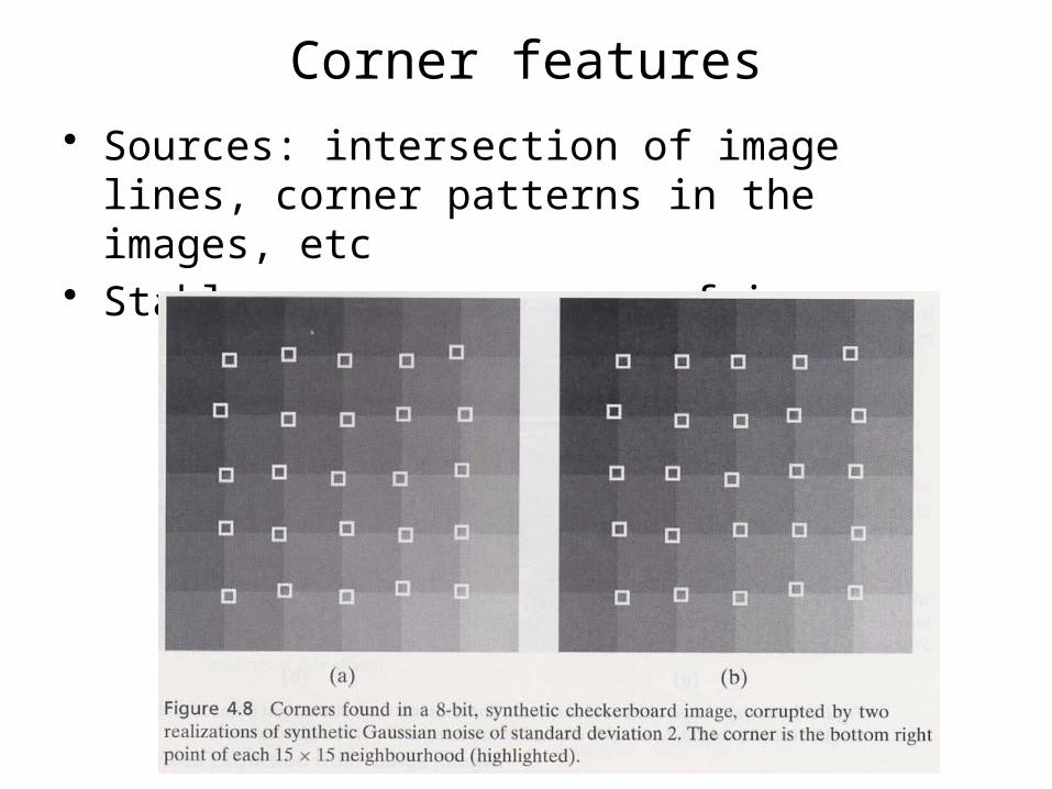
Corner features
• Sources: intersection of image lines, corner patterns in the images, etc
• Stable across sequence of images
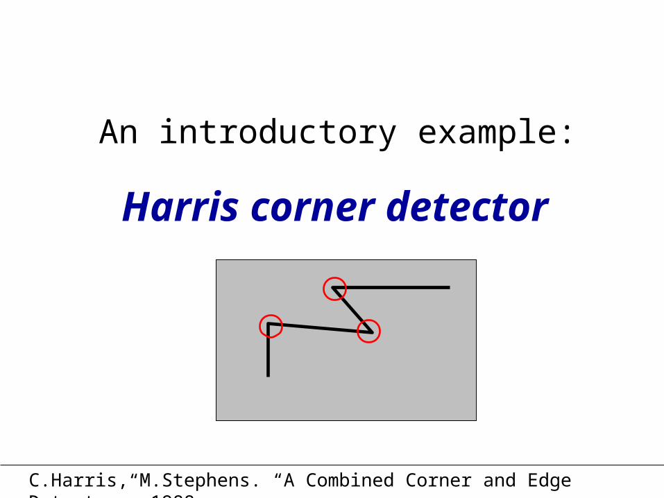
An introductory example:
Harris corner detector
C.Harris, M.Stephens. “A Combined Corner and Edge Detector”. 1988

The Basic Idea
• We should easily recognize the point by looking through a small window
• Shifting a window in any direction should give a large change in intensity

Harris Detector: Basic Idea
“flat” region:no change in all directions
“edge”:no change along the edge direction
“corner”:significant change in all directions

Harris Detector: Mathematics
2
,
( , ) ( , ) ( , ) ( , )x y
E u v w x y I x u y v I x y
Window-averaged change of intensity for the shift [u,v]:
IntensityShifted intensity
Window function
orWindow function w(x,y) =
Gaussian1 in window, 0 outside
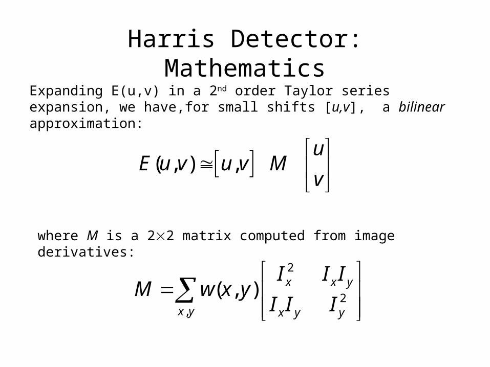
Harris Detector: Mathematics
( , ) ,u
E u v u v Mv
Expanding E(u,v) in a 2nd order Taylor series expansion, we have,for small shifts [u,v], a bilinear approximation:
2
2,
( , ) x x y
x y x y y
I I IM w x y
I I I
where M is a 22 matrix computed from image derivatives:
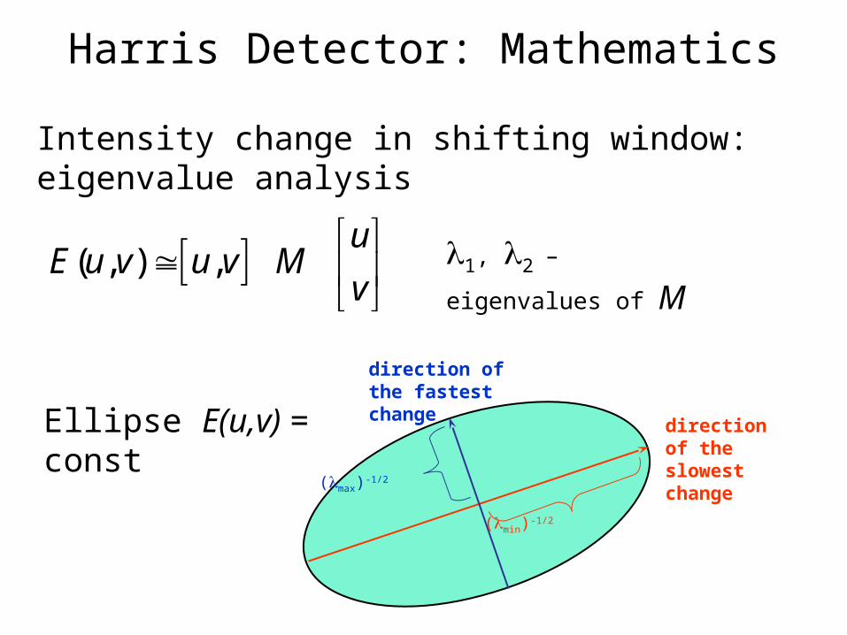
Harris Detector: Mathematics
( , ) ,u
E u v u v Mv
Intensity change in shifting window: eigenvalue analysis
1, 2 – eigenvalues of M
direction of the slowest change
direction of the fastest change
(max)-1/2
(min)-1/2
Ellipse E(u,v) = const

Selecting Good Features
l1 and l2 are large

Selecting Good Features
large l1, small l2
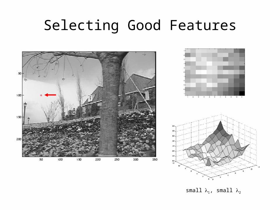
Selecting Good Features
small l1, small l2
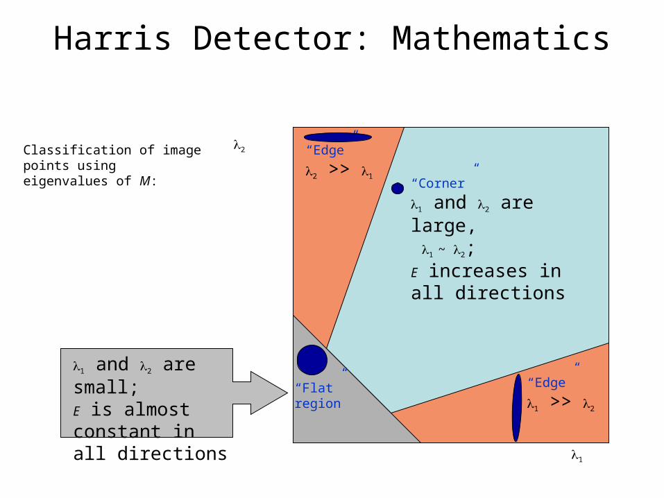
Harris Detector: Mathematics
1
2
“Corner”
1 and 2 are large, 1 ~ 2;E increases in all directions
1 and 2 are small;E is almost constant in all directions
“Edge”
1 >> 2
“Edge”
2 >> 1
“Flat” region
Classification of image points using eigenvalues of M:

Harris Detector: Mathematics
Measure of corner response:
2det traceR M k M
1 2
1 2
det
trace
M
M
(k – empirical constant, k = 0.04-0.06)

Harris Detector: Mathematics
1
2“Corner”
“Edge”
“Edge”
“Flat”
• R depends only on eigenvalues of M
• R is large for a corner
• R is negative with large magnitude for an edge
• |R| is small for a flat regionR > 0
R < 0
R < 0|R| small
Harris Detector
• The Algorithm:– Find points with large corner response function R (R
> threshold)– Take the points of local maxima of R

Harris Detector: Workflow
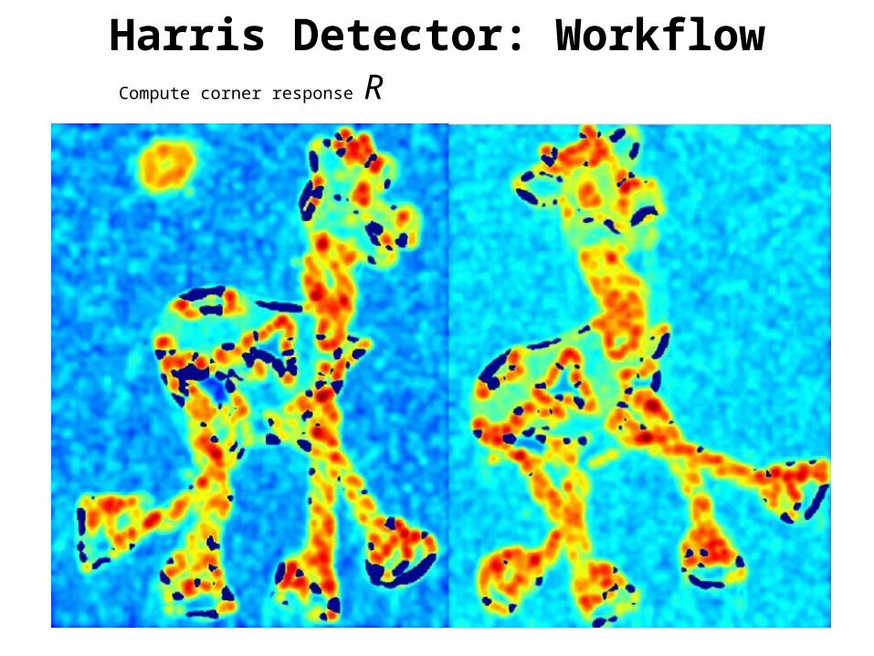
Harris Detector: WorkflowCompute corner response R
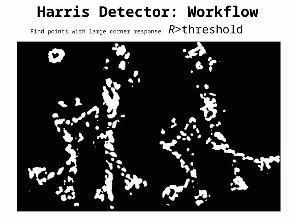
Harris Detector: WorkflowFind points with large corner response: R>threshold
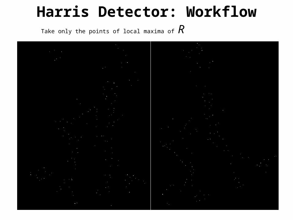
Harris Detector: WorkflowTake only the points of local maxima of R

Harris Detector: Workflow

Harris Detector: Summary
• Average intensity change in direction [u,v] can be expressed as a bilinear form:
• Describe a point in terms of eigenvalues of M:measure of corner response
• A good (corner) point should have a large intensity change in all directions, i.e. R should be large positive
( , ) ,u
E u v u v Mv
2
1 2 1 2R k
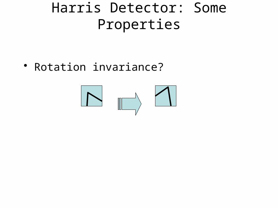
Harris Detector: Some Properties
• Rotation invariance?

Harris Detector: Some Properties
• Rotation invariance
Ellipse rotates but its shape (i.e. eigenvalues) remains the same
Corner response R is invariant to image rotation

Harris Detector: Some Properties
• Invariance to image intensity change?

Harris Detector: Some Properties
• Partial invariance to additive and multiplicative intensity changes
Only derivatives are used => invariance to intensity shift I I + b
Intensity scale: I a I
R
x (image coordinate)
threshold
R
x (image coordinate)

Harris Detector: Some Properties
• Invariant to image scale?

Harris Detector: Some Properties
• Not invariant to image scale!
All points will be classified as edges
Corner !

We want to:
detect the same interest points regardless of image changes

Models of Image Change
• Geometry– Rotation– Similarity (rotation + uniform scale)
– Affine (scale dependent on direction)valid for: orthographic camera, locally planar object
• Photometry– Affine intensity change (I a I + b)

Rotation Invariant Detection
• Harris Corner Detector
C.Schmid et.al. “Evaluation of Interest Point Detectors”. IJCV 2000
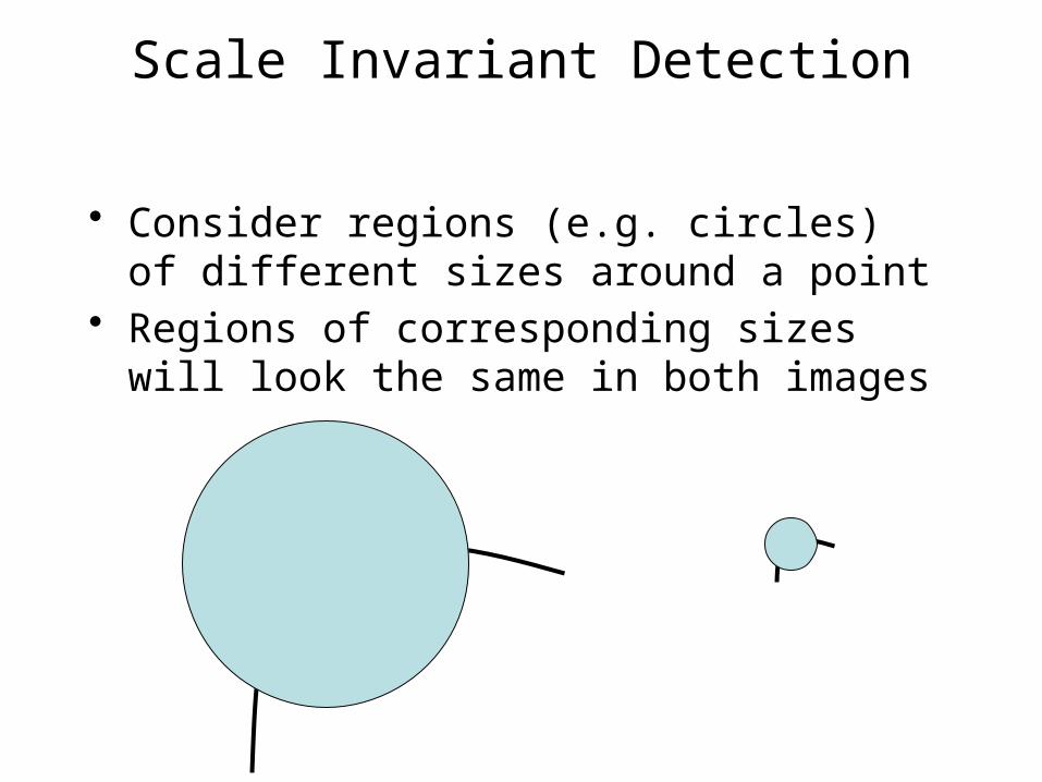
Scale Invariant Detection
• Consider regions (e.g. circles) of different sizes around a point
• Regions of corresponding sizes will look the same in both images

Scale Invariant Detection
• The problem: how do we choose corresponding circles independently in each image?
Scale Invariant Detection
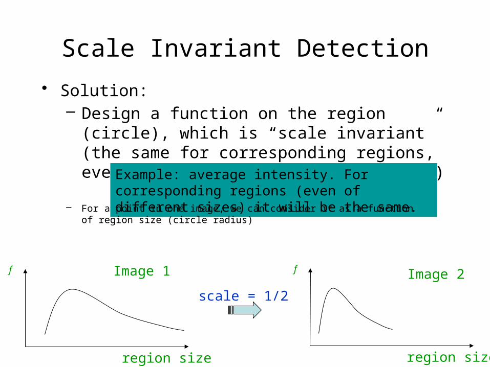
• Solution:– Design a function on the region (circle), which is
“scale invariant” (the same for corresponding regions, even if they are at different scales)
Example: average intensity. For corresponding regions (even of different sizes) it will be the same.
scale = 1/2
– For a point in one image, we can consider it as a function of region size (circle radius)
f
region size
Image 1 f
region size
Image 2
Scale Invariant Detection
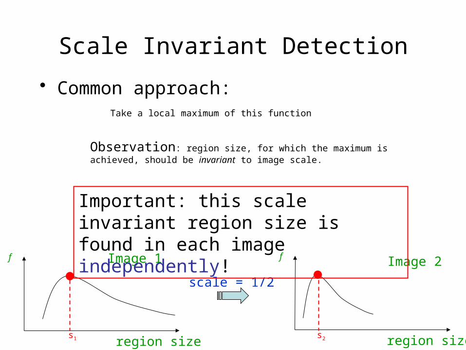
• Common approach:
scale = 1/2
f
region size
Image 1 f
region size
Image 2
Take a local maximum of this function
Observation: region size, for which the maximum is achieved, should be invariant to image scale.
s1 s2
Important: this scale invariant region size is found in each image independently!

Scale Invariant Detection
• A “good” function for scale detection: has one stable sharp peak
f
region size
bad
f
region size
bad
f
region size
Good !
• For usual images: a good function would be a one which responds to contrast (sharp local intensity change)

Scale Invariant Detection
• Functions for determining scale
2 2
21 22
( , , )x y
G x y e
2 ( , , ) ( , , )xx yyL G x y G x y
( , , ) ( , , )DoG G x y k G x y
Kernel Imagef Kernels:
where Gaussian
Note: both kernels are invariant to scale and rotation
(Laplacian)
(Difference of Gaussians)


Scale Invariant Detection: Summary
• Given: two images of the same scene with a large scale difference between them
• Goal: find the same interest points independently in each image
• Solution: search for maxima of suitable functions in scale and in space (over the image)
Methods:
1. Harris-Laplacian [Mikolajczyk, Schmid]: maximize Laplacian over scale, Harris’ measure of corner response over the image
2. SIFT [Lowe]: maximize Difference of Gaussians over scale and space

Point Descriptors
• We know how to detect points• Next question: How to match them?
?
Point descriptor should be:1. Invariant2. Distinctive

SIFT – Scale Invariant Feature Transform1
• Empirically found2 to show very good performance, invariant to image rotation, scale, intensity change, and to moderate affine transformations
1 D.Lowe. “Distinctive Image Features from Scale-Invariant Keypoints”. Accepted to IJCV 20042 K.Mikolajczyk, C.Schmid. “A Performance Evaluation of Local Descriptors”. CVPR 2003
Scale = 2.5Rotation = 450

CVPR 2003 Tutorial
Recognition and Matching Based on Local Invariant Features
David Lowe
Computer Science Department
University of British Columbia

Invariant Local Features• Image content is transformed into local feature
coordinates that are invariant to translation, rotation, scale, and other imaging parameters
SIFT Features
Advantages of invariant local features
• Locality: features are local, so robust to occlusion and clutter (no prior segmentation)
• Distinctiveness: individual features can be matched to a large database of objects
• Quantity: many features can be generated for even small objects
• Efficiency: close to real-time performance
• Extensibility: can easily be extended to wide range of differing feature types, with each adding robustness

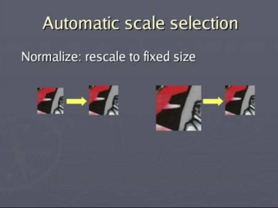
Scale invariance
Requires a method to repeatably select points in location and scale:
• The only reasonable scale-space kernel is a Gaussian (Koenderink, 1984; Lindeberg, 1994)
• An efficient choice is to detect peaks in the difference of Gaussian pyramid (Burt & Adelson, 1983; Crowley & Parker, 1984 – but examining more scales)
• Difference-of-Gaussian with constant ratio of scales is a close approximation to Lindeberg’s scale-normalized Laplacian (can be shown from the heat diffusion equation)
B l u r
R e s a m p l e
S u b t r a c t
B l u r
R e s a m p l e
S u b t r a c t
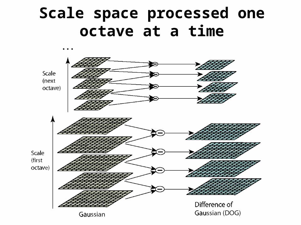
Scale space processed one octave at a time

Key point localization
• Detect maxima and minima of difference-of-Gaussian in scale space
• Fit a quadratic to surrounding values for sub-pixel and sub-scale interpolation (Brown & Lowe, 2002)
• Taylor expansion around point:
• Offset of extremum (use finite differences for derivatives):
B l u r
R e s a m p l e
S u b t r a c t

Select canonical orientation
• Create histogram of local gradient directions computed at selected scale
• Assign canonical orientation at peak of smoothed histogram
• Each key specifies stable 2D coordinates (x, y, scale, orientation)
0 2
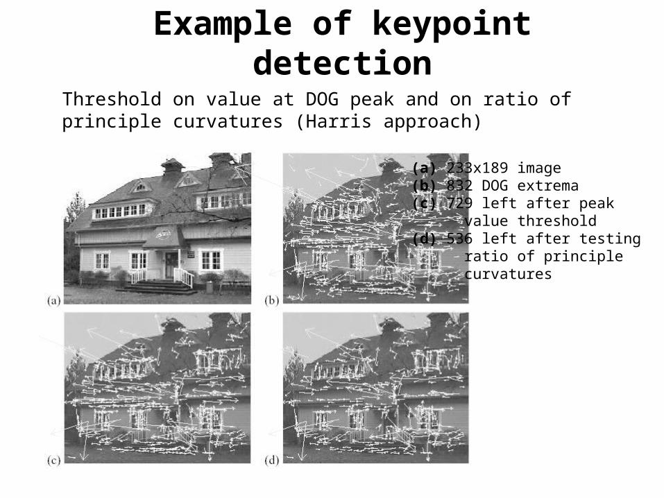
Example of keypoint detection
Threshold on value at DOG peak and on ratio of principle curvatures (Harris approach)
(a) 233x189 image(b) 832 DOG extrema(c) 729 left after peak value threshold(d) 536 left after testing ratio of principle curvatures

SIFT vector formation• Thresholded image gradients are sampled over
16x16 array of locations in scale space• Create array of orientation histograms• 8 orientations x 4x4 histogram array = 128
dimensions
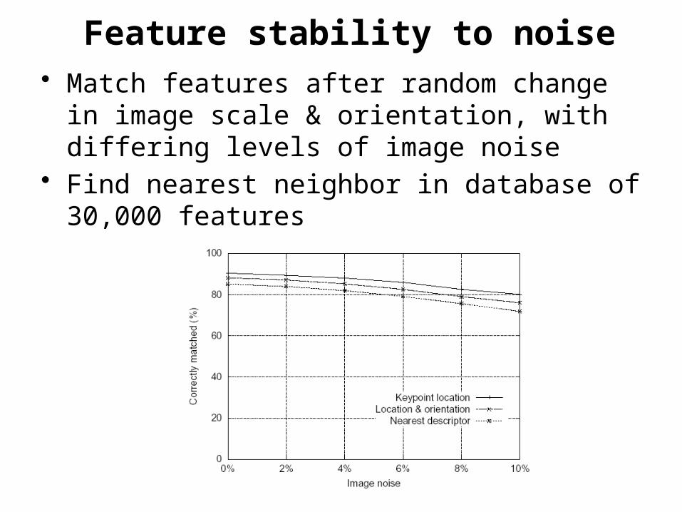
Feature stability to noise• Match features after random change in image
scale & orientation, with differing levels of image noise
• Find nearest neighbor in database of 30,000 features
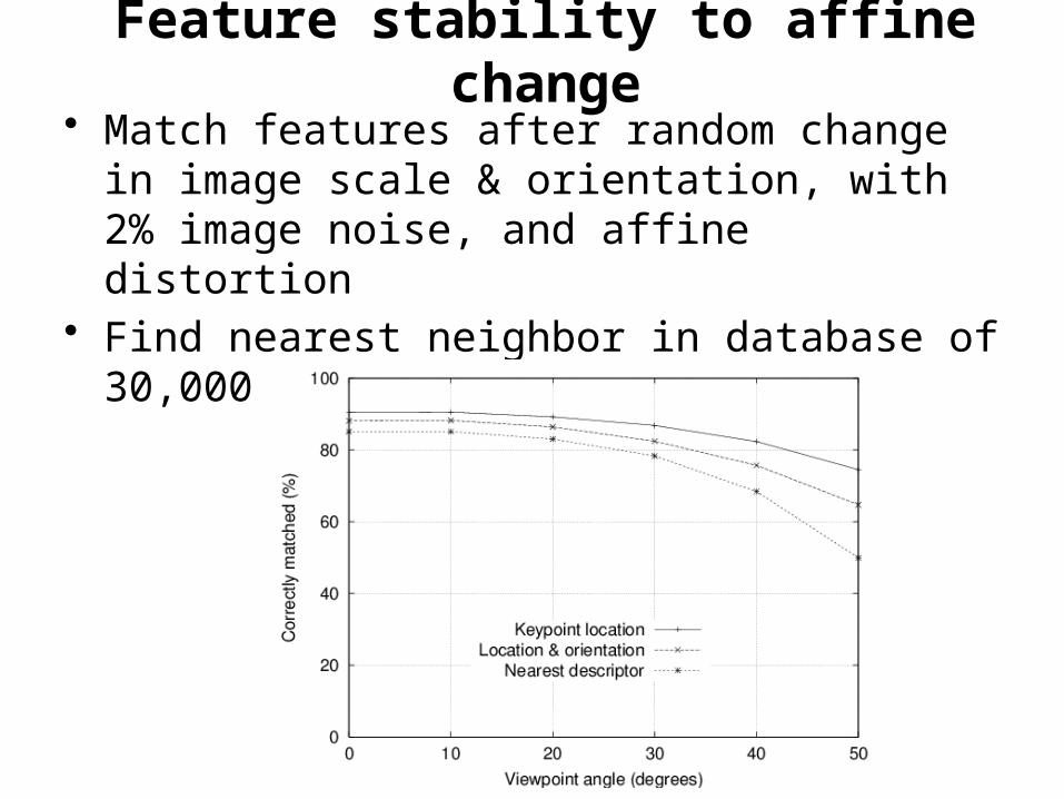
Feature stability to affine change• Match features after random change in image
scale & orientation, with 2% image noise, and affine distortion
• Find nearest neighbor in database of 30,000 features

Distinctiveness of features• Vary size of database of features, with 30 degree
affine change, 2% image noise• Measure % correct for single nearest neighbor
match


A good SIFT features tutorial
http://www.cs.toronto.edu/~jepson/csc2503/tutSIFT04.pdf
By Estrada, Jepson, and Fleet.
Other References
• Harris & Stephens (1988)http://www.bmva.org/bmvc/1988/avc-88-023.pdf
• Lowe (2004)http://www.cs.ubc.ca/~lowe/papers/ijcv04.pdf
• Mikolajczyk & Schmid (2005)http://lear.inrialpes.fr/pubs/2005/MS05/mikolajczyk_pami05.pdf
• Brown & Lowe (2007)http://cvlab.epfl.ch/~brown/papers/ijcv2007.pdf