2
Family Composition and Off-Farm Participation Decisions in
Israeli Farm Households*
By
Ayal Kimhi Department of Agricultural Economics and Management
Faculty of Agriculture, The Hebrew University P.O. Box 12, Rehovot 76100, Israel
November 2001
ABSTRACT
This paper studies the dependence of the off-farm participation behavior of farm
operators and their spouses on the demographic composition of the household.
Specifically, we focus on farm families without parents, siblings or partners,
and examine the effects of the existence and work decisions of elderly children
of the farm couple. We find that both the father and the mother tend to reduce
their participation in off-farm work as the number of elderly children rises. This
result holds even after controlling for observed characteristics. We also find that
the effect of elderly children stems from considerations related to both farm
production and household production.
_____________________
* This research was supported in part by Research Grant Award No. IS-2762-96 from BARD - the United States � Israel Binational Agricultural Research and Development Fund. We thank the Central Bureau of Statistics in Israel, and especially Elana Dror and Haim Regev, for providing the data.
3
Introduction
The time allocation decision of farmers has long attracted researchers because many
farmers divide their labor supply between farm work and off-farm work, a phenomenon that is
rarely observed in other sectors of the economy (Shishko and Rostker 1976). Other than the
scientific attractiveness of multiple job-holding among self-employed farmers, understanding
this phenomenon is important for the design of agricultural policy, and, more generally, rural
policy. Many policy instruments are aimed at improving farm income or reducing its variability.
Policy makers often do not fully appreciate the importance of earnings from off-farm sources
that supplement farm income and serve as a buffer against farm income fluctuations. Moreover,
any farm-related policy should take into account the ability of farmers to act on the extensive
margin between farming and off-farm activities in addition to their actions on the intensive
margin between different farm activities. Understanding how farmers allocate their time
between farming and off-farm occupations is therefore crucial for designing successful farm
policies.
The empirical attempts to analyze farmers� time allocation decisions have thus far been
limited to husband and wife only because of two main reasons. One is the lack of sufficient data
on the time allocation of other family members. The other is the limitation imposed by the
availability of suitable econometric techniques. As family farming is still dominant in
agricultural sectors all over the world, data on farm households are readily available in many
countries. This research will use data from a detailed family farm survey conducted in Israel,
which include the time allocation patterns of all farm-family members older than 14 years.
Econometric tools such as quasi-maximum likelihood estimation (Kimhi 1994), and minimum
distance estimation (Kimhi and Lee 1996), enable the joint estimation of a large number of
participation and labor supply equations. Hence the purpose of this research is to extend the time
allocation analysis to other members of the farming family.
Previous research (Kimhi 1996) has found that household composition affects the
tendency of different household members to provide off-farm labor. This is explained by the
differential income effects resulting from the household�s joint budget constraint, and by the
time and money costs imposed by different household members. In particular, farm couples are
more likely to work off the farm when the number of other adults in the household increases.
This paper builds on the previous work and modifies it in several directions: (a) a more recent
data set is used; (b) we focus on farm families without parents, siblings or partners, so the only
other adults in the household are the immediate descendents of the farm couple (and the
4
descendents� spouses); (c) we estimate the off-farm participation equations of the descendents
jointly with the off-farm participation equations of the farm couple.
We find that the effect of household composition on the off-farm participation behavior
of the farm couple is completely different than the behavior indicated by the previous results. In
particular, we find that the farm couple is less likely to work off the farm as the number of adult
children in the household rises. We also explore two possible reasons for this behavior, one
related to complementarity of farm labor inputs of different family members, and another
related to the time burden in household production imposed by adult children. Both reasons are
supported by the empirical results.
The following section starts with a survey of previous literature. Then we present a
theoretical model of time allocation and off-farm labor participation in a household context.
After that we discuss the empirical methods we adopt for this analysis. The following sections
present the data, descriptive statistics, and empirical results. The last section provides a
summary and conclusions.
Background and Previous Results
The literature is rich in applications of the agricultural household model to time
allocation problems. The traditional approach has been to estimate off-farm participation
equations and labor supply equations of farm operators (e.g., Sumner 1982). In the last decade,
researchers have moved to estimate two-equation models in which the off-farm labor supply
equations of husbands and wives are jointly determined (e.g., Huffman and Lange 1989; Tokle
and Huffman 1991; Lass and Gempesaw 1992). The results of these studies indicated that off-
farm labor supply of husbands and wives are positively correlated. Recently, this approach has
been extended to include farm work participation equations (Kimhi 1994) and labor supply
equations as well (Kimhi and Lee 1996). Buttel and Gillespie (1984) have also found that men's
and women's farm and off-farm labor supply decisions are correlated.
However, farm families are not made of a husband and a wife only. On the contrary,
farm families are often larger than non-farm families, including several generations who
function as an extended family. The importance of within-family succession serves as an
incentive for adult children to work together with their parents on the family farm (Kimhi 1995).
Blanc and Perrier-Cornet (1993) found that European successors often work as laborers for their
parents for ten years or more before receiving ownership. Hence, the existence of other family
members allows the farm operator and spouse to have more flexibility in their time allocation
decisions.
5
This claim is supported by the empirical results of Kimhi (1996), who studied the effect
of family composition on the labor participation decisions of Israeli farm couples. Children
under 3 years of age decreased the tendency of spouses to participate in either farm work or off-
farm work, decreased operators' farm participation but increased their off-farm participation.
Older children (up to 18 years of age) increased farm participation and decreased off-farm
participation of both adult family members. The number of other adults (19 to 51 years old)
increased (decreased) off-farm (farm) participation of both spouses. It seems that other adults
are net substitutes in farm work. Further, a measure of other adults' farm work was included as
an explanatory variable, and the results did not change much, though the coefficients tended to
be larger in absolute value. This variable had a strong positive (negative) effect on farm (off-
farm) participation probability. Finally, the joint participation model was estimated separately
for households with and without other adults. The results implied that the time allocation of
farm operators and their spouses depends strongly on the existence of other adult household
members.
Overall, these results indicate that there are substitutability and complementarity
relations between the labor supplies of different household members to the two sectors. Hence, a
joint estimation is desirable.
Theory
Up to the present, the time-allocation decisions in family farms were modeled as if they
are derived from a joint household utility model, that is, each and every family member acts so
as to maximize a utility function defined over consumption and leisure of all family members.
This is the framework used by Huffman (1991) in his comprehensive theoretical survey of the
farm-household models. Kimhi (1994) suggested a slight modification of the theory to allow for
zero farm work. The resulting model is outlined in short below.
Assume that household utility (U) is a function of household consumption (C) and the
vector of household members' home time, Th (housework and leisure). Each household member
can use his time endowment (T) for farm work (Tf), market work (Tm), and/or home time.
Hence, the time constraint is (in vector notation):
(1) Tf + Tm + Th = T.

6
Non-negativity constraints are imposed on market work and farm work of each household
member: Tf ≥ 0 and Tm ≥ 0. Consumption is constrained by household income, which is
composed of: (i) farm income (Yf), which is a function of each household member's farm labor
supply; (ii) off-farm labor income, which is the sum of off-farm earnings of all household
members (Ymi); and (iii) other income (Yo). The resulting budget constraint is:
(2) C = Yf(Tf ;Zf)+ ΣiYmi(Tmi ;Zmi)+ Yo.
The household optimization problem is to maximize U(C, Th; Zu) subject to the time,
budget, and non-negativity constraints, where Zj are exogenous shifters of function j. The
optimal solution is characterized by the Kuhn-Tucker conditions, which are the first-order
conditions for maximizing the Lagrange function:
(3) U(C ,Th; Zu) + λ⋅[Yf (Tf; Zf) + ΣiYmi (Tmi; Zmi) + Yo - C] +
+ µµµµt⋅[T - Tf - Tm - Th] + µµµµf⋅Tf + µµµµm⋅Tm
over {C, Th, Tf, Tm} and minimizing it over {λ, µµµµt, µµµµf, µµµµm}. The farm work and off-farm work
participation conditions are, respectively, a subset of the Kuhn-Tucker conditions:
(4) ∂∂∂∂Yf /∂∂∂∂Tf ≤ µµµµt /λ
(5) ∂∂∂∂Ym /∂∂∂∂Tm ≤ µµµµt /λ
(in vector notation), where µµµµt = ∂∂∂∂U/∂Th and λ = ∂U /∂C. Participation (an internal solution)
occurs when the equality holds.
If an interior solution occurs for all choices (all household members work both on and
off the farm), the participation equations and all the constraints can be solved for endogenous
variables {C, Th, Tf, Tm, λ, µµµµt, µµµµf, µµµµm} as functions of all the exogenous variables Zu, Zf, Zm, Yo,
and T. This is the reduced-form solution. Using this solution in the participation equations, we
can then determine which of the labor participation conditions is satisfied. If n is the number of
potential workers in the household, there are 2n participation equations, taking the forms:
(4)� fj (Zu, Zf, Zm, Yo, T) ≤ g (Zu, Zf, Zm, Yo, T), j=1...n;
7
(5)� hj (Zmj) ≤ g (Zu, Zf, Zm, Yo, T), j=1...n.
The model can easily be extended to include housework as an activity separate from
leisure, as well as non-agricultural self-employment activities of the household. The results of
this model could hold even if the strong assumption of a single household utility function is
relaxed. According to Becker's (1991) "Rotten Kid Theorem", if each household member
maximizes his own utility function, but one member is sufficiently altruistic towards the others,
and this member controls a sufficient amount of resources, the behavior of all household
members will be similar to the case of a single joint utility function.
Equation (5)�, the off-farm labor participation equation, is of most interest for our
purposes. We can see that each household member�s off-farm participation decision depends on
the characteristics of all other household members, through the right-hand side of (5)�. It is this
dependence that we examine in this paper.
Empirical Methods
Off-farm participation models with up to two participation equations were modeled by
maximum likelihood models in most of the studies of joint husband-wife work decisions. The
quasi maximum likelihood approach can be used for more than two equations. The following
description of the quasi maximum likelihood method is based on Kimhi (1994).
Using a first-order approximation of (5)�, and adding stochastic terms for the
approximation errors, we can write a generic empirical off-farm participation equation as a
linear function of the explanatory variables:
(5)�� ββββujZu + ββββfjZf + ββββmjZm + βojYo + ββββtjT + εj ≤ 0 (j=1...n),
where the β's are unknown parameters. Strict inequality indicates nonparticipation. If εj ~
N(0,1), each equation can be estimated by probit. Assuming a general correlation structure
between the equations necessitates a joint estimation procedure in order to exploit all available
information and provide efficient estimators. This correlation structure could result, for
example, from unobserved household-level variables that are common to all equations.
Multivariate probit ML estimation of more than two equations requires more than two
levels of numerical integration, making the task impractical. Instead, in the Quasi-ML method,
restrictions are imposed on the parameters in order to simplify the likelihood function. The
8
restrictions are chosen such that the restricted model satisfies the orthogonality conditions,
which are equivalent to the first-order conditions of the restricted ML model. The simplest
version of this class is estimating each equation separately by probit, then estimating the cross-
equation correlation coefficients in a second stage by using bivariate probit on each possible pair
of equations, replacing the ββββ parameters by their first-stage estimators.
The method is illustrated here for the case of four equations. Let the probit equations be
ααααi⋅Xi + νi ≤ 0 (i=1,2,3,4), where strict equality indicates participation. Assume the first stage
probit estimators are αααα*i (i=1,2,3,4). The second stage involves maximizing a bivariate probit
log-likelihood function of the form £ij = Σ ln B(diαααα*iXi, djαααα*
jXj, dijρij), with respect to ρij, for
each possible (i,j) ∈ {(1,2), (1,3), (1,4), (2,3), (2,4), (3,4)}. Summation is over individuals; B is
the bivariate normal probability function; ρij is the correlation between νi and νj; Ik equals one if
participation occurs, zero otherwise; and di=2Ii-1 and dij=didj. Since maximizing £ij for each
possible (i,j) is equivalent to maximizing £ = £12 + £13 + £14 + £23 + £24 + £34, £ can be
maximized over all the parameters in one stage. This is the most efficient QML estimator
subject to the condition that the level of integration is not higher than two. The method is
appropriate for any number of equations. The true covariance matrix of the estimators should be
calculated as H -1WH -1 where H is the matrix of second derivatives of quasi-likelihood function
£ and W is its gradient outer-product matrix.
Data
The data come from a farm survey that was conducted in Israel in 1995 (State of Israel,
Central Bureau of Statistics 1998). The survey encompassed a representative 10% sample of
farms, and included approximately 3000 farms of various kinds. Three separate sectors were
surveyed: Moshavim (cooperative villages), other Jewish localities, and Arab localities. Note
that despite the cooperative structure of Moshavim, these farms can be treated as private family
farms for all practical purposes.1 Sampling in each sector was conducted in two stages: localities
were sampled in the first stage out of all localities in the sector. Then, individual farms were
sampled in the second stage. Each sample was stratified according to farm size, branch, and
region, and an appropriate weight was attached to each observation.
The survey questionnaire included very detailed questions about farm production
activities, both in 1995 and in 1990, as well as personal and family characteristics (age,
education, tenure, ethnic origin). Regarding time allocation, each family member was asked if
he/she engaged in agricultural activities on the farm up to 1/4 of a full-time job, up to 1/2, 3/4,
9
full time, or not at all. A similar question was asked about non-agricultural farm activities, and
about off-farm work.
We use only a small subset of the variables in this data set. Among the time allocation
variables, we only use a dummy for working/not working in each sector, and ignore the level of
work. This is because the vast majority of those who work off the farm do it on a full-time basis.
Also, we add together those who work off the farm and those who participate in non-agricultural
activities on the farm, because the latter are a very small group. Other personal characteristics
that we use are age, a dummy for being born in Israel, a dummy for having an ethnic origin in
Asia or Africa (this relates to the respondent or his/her father), and three educational dummies:
one for finishing high school, one for having more than high school education, and one for
having some kind of agricultural education. The latter dummy variable is independent of the
former two dummies, in the sense that finishing agricultural high school qualifies for both the
first and the third dummies.
Family-related variables include two locality-type dummies (private-Jewish and Arab,
excluded group is Moshavim), two location dummies (north and south, excluded location is
center), the number of children up to age 14, the number of adolescents up to age 21, and
dummies for the number of adults in the household: group=1 is for husband and wife only,
group=2 is for husband, wife, and one adult child, group=3 is for husband, wife, and two adult
children (or an adult child and his/her spouse), and group=4 is for husband, wife, and more than
two adult children or spouses. An adult child is a child older than 21 years.2 Other types of
households, including single-parent households, households with elderly parents, and other
forms of extended families, were excluded from the current analysis. There were 1949 families
left in the data set comprising of groups 1 to 4.
Variables related to the farm operator include tenure, which is the time since the current
owner operates the farm, and two dummies for method of receiving the farm, one for succession
and one for purchase (the excluded group includes those who received the farm through the
settlement agencies). Variables related to farm production include level of specialization, land,
capital, and types of products. Level of specialization includes two dummy variables: one for
specialized farms, in which one branch accounts for at least 90% of total value added,3 and
another for diversified farms, which include all other farms with positive production. The
excluded group includes inactive farms. Land size includes all the land that is permanently held
by the farm.4 Capital stock is the value of buildings, machinery, equipment, and livestock.5 We
also include dummy variables indicating production in each of the following branches: flowers
and nurseries, poultry, field crops and vegetables, and cattle.6
10
Descriptive Statistics
Table 1 includes descriptive statistics of the personal characteristics of the different
household members.7 We can see that overall, 55% of the operators and 46% of the spouses
work off the farm, while 69% of oldest children do so. However, the fraction of operators and
spouses who work off the farm declines with the number of adult children in the household,
while that of the oldest children rises. This could very well be an age effect. As can be seen from
the table, the ages of operators, spouses, and oldest children rise with the number of adult
children, reflecting life-cycle effects. While the parents are already in the age range in which the
tendency to work off the farm declines with age, the children are not. Opposite to the results of
Kimhi (1996), we do not find that adult children substitute for their parents� farm labor. On the
contrary, fathers� farm labor participation rises with the number of adult children, while that of
the mother doesn�t change monotonically. This could be due to several reasons. First, Kimhi
(1996) treated all adult household members equally, while here we only deal with immediate
descendents. Second, only 24% of oldest children work on the farm, reflecting the highly
diminished role of agriculture in rural Israel in 1995 relative to 1981. Finally, these are only raw
results; we have to see whether they still hold after we control for observed differences among
the groups of households, especially age.
The fraction of operators and spouses who were born in Israel declines sharply as the
number of adult children increases, and so does the fraction of those of Asian or African origin.
This is most likely a reflection of the age pattern, as well, since most immigration to Israel, and
especially from Asia and Africa, occurred in the early 1950s. Among adult children, these
variables do not vary systematically across the groups of households. Education does not vary
systematically across the groups for males and children, but declines with the number of adult
children for females. This is likely to be a cohort effect. Agricultural-specific education does not
seem to be very common in this sample. It is interesting to note that 69% of adult children are
males. This could be due to two reasons. First, children�s spouses are also included when
present, and male spouses of female children are likely to be older. Second, there could be a
higher tendency for male children to live on the family farm alongside their parents, for farm
succession purposes.
Table 2 includes descriptive statistics of the operator, family, and farm variables. We
can first observe that private Jewish farm families are less likely to have adult children on the
farm, while Arab farm families are more likely to have three or more adult children on the farm.
This probably reflects a lower incentive for farm succession in private Jewish family farms on
11
one hand,8 and the different fertility and marriage behavior in Arab families on the other hand.
The majority of groups 1 and 2 are found in the north and south of the country, while the
majority of groups 3 and 4 are found in central locations. This can be explained by the
residential value of living on the farm, which is much higher in central regions due to higher
housing prices. The number of adolescents goes up from group 1 to group 2 and then declines,
while the number of younger children goes down from group 1 to group 2 and then rises. This
reflects the fact that households with a single adult child are in a more advanced stage in the life
cycle than households without an adult child, as we have learned from the age statistics.9 The
opposite is observed when moving from group 2 to groups 3 and 4. Here the increase in the
number of young children is perhaps due to the third generation.
Average tenure increases monotonically from group 1 to group 4, again reflecting the
stage in the life cycle. The fraction of operators who have succeeded their parents on the farm
does not change much with the number of adult children, while the fraction of operators who
have purchased their farms from previous owners declines monotonically from group 1 to group
4. This perhaps reflects the fact that most Moshavim have been established between the late
1940s and the early 1950s, so older operators are more likely to have obtained their farms
directly from the settlement institutions.
The fractions of specialized and diversified farms do not change monotonically from
group 1 to group 4, but the fraction of inactive farms (the excluded category) decreases
monotonically. It could be that inactive farms are less attractive to adult children for succession
purposes, and it could also be that farms without successors become inactive. The causality is
not clear here. Landholdings don�t change much from group 1 to group 4. Capital stock, on the
other hand, rises. This difference is due to the fact that landholdings, at least in Moshavim, were
determined at time of establishment, while capital stock was gradually accumulated over the
years since establishment. The positive association between capital stock and number of adult
children residing on the farm can be explained similarly to the explanation of the level of
inactivity above, again without the ability to determine causality. Regarding the branch
dummies, we do observe variations across the groups of households. Group 4, for example, has
more field crops and less flowers than the other groups. Group 1 has less poultry and group 3
has flowers. We do not good explanations for these variations.
Results
We first apply the quasi-maximum likelihood estimation of the off-farm participation
equation to the whole sample, allowing for different intercepts for the different groups of

12
households. The model includes 3 different equations: for the male operator or spouse, for the
female operator or spouse, and for the oldest adult child. We tried to add an equation for a
second adult child, but the model did not converge, probably because the number of
observations with more than one adult child was not large enough. The estimation was
performed using Gauss.10 The procedure accounts for the different probability weights attached
to different households, and for missing values. Most cases of missing values were in the work
participation variables: many respondents did not answer these questions. While we believe that
a large fraction of those thought the questions were not relevant for them because they did not
work at all, there is no way to confirm this, and hence we exclude these individuals from the
model by attaching zero weights. A few additional observations were excluded because of
missing schooling data.11
The results are in table 3. We first observe that the three off-farm participation equations
are positively correlated. This could be due to two reasons. First, it could be that unobserved
household-specific components are important determinants of off-farm labor participation, even
after controlling for all the observed attributes. Second, it could be easier for other household
members to work off the farm when one member already does so, for various reasons.12 The
group dummies have negative coefficients in the males� equation, but only the coefficient of
group 4 is statistically significant. On the other hand, all of the group dummies have
significantly negative coefficients in the females� equation, implying that the tendency of farm
women to work off the farm is smaller when adult children are present. This is similar to the raw
statistics in table 1. The tendency of the oldest adult child to work off the farm increases with
the number of adult children, but, as in the case of the father, only the coefficient of group 4 is
statistically significant.
Age has a typical inverted U effect on participation probability. Females are more likely
to work off the farm if they were born in Israel. This variable is considered as a proxy for
country-specific human capital that affects potential earnings positively. Ethnic origin has a
significant effect in the children�s equation only. Children with Asian or African origin are more
likely to work off the farm. Education has a positive effect on males� participation, as expected,
but does not affect off-farm participation of females or children. Participation is lower in
northern and southern regions, as in the raw statistics. Both north and south dummies are
significant in the females� equation, while only the south dummy is significant in the males�
equation. None of the regional dummies was significant in the children�s equation. The number
of children has a negative effect on participation, but the effect is significant only for females.
This is similar to the result of Kimhi (1996) that children impose a time cost on the family

13
members, especially the mother. The number of adolescents did not have significant effects in
any of the equations.
Tenure does not have a significant effect on the off-farm labor participation decision.
Participation is more likely in farms purchased from a previous owner, except for the case of
females. This hints to the existence of a phenomenon of purchasing farms for residential
purposes. The level of farm specialization does not seem to have an effect on the off-farm
participation decision, but the male operators of active farms are much less likely to work off
the farm than the male operators of inactive farms. This is a natural result stemming from the
lower value of reservation wage on inactive farms. Landholdings have a significantly positive
effect on the female�s probability of working off the farm. This is a surprising result. If land
were important as a factor of production, we would have expected the opposite. It may be that
land-intensive farms do not provide employment opportunities for females. Capital stock, on the
other hand, has a significantly negative effect on the off-farm participation probabilities of all
household members, as expected. Males� participation was lowest in the presence of field crops
or vegetables, the second lowest in flower farms, the third � in poultry farms, and the fourth � in
cattle farms This is compared to fruit farms. The same rankings are observed for females, except
for the fact that cattle farms are not significantly different from fruit farms. None of the branch
dummies was significant in the children�s equation.
Male operators of private Jewish farms are less likely to work off the farm than those in
Moshavim. This is attributed to the institutional link between farm residence and farm operation
in Moshavim (Kimhi 1998) that counts people in Moshavim as farm operators even when the
farm is inactive. When we repeat the estimation with active farms only, the coefficient of private
Jewish farms is no longer significant.13 In Arab farm families, females and children are less
likely to work off the farm. This may be due to differences in cultural tradition but also to off-
farm labor market discrimination.
Next, we want to examine the importance of the constraint imposed on the previous
model, that the participation equations in the different groups of households are only different in
their intercepts. For this, we estimate the model separately in each of the groups of households.
The model of group 1 includes only two equations, so it is in fact a bivariate probit model. The
model of group 4 did not converge, probably due to the relatively small number of observations.
Hence we estimated the model for groups 3 and 4 together, allowing for a different intercept for
each of the groups, as before. The results are reported in table 4. A quick look at the table
reveals that the coefficient estimates vary considerably across the groups of households. One
interesting change is that agricultural education significantly decreases the tendency of adult
14
males to work off the farm, except for farmers of group 1. All the correlation coefficients are
still positive and significant, indicating the importance of a joint analysis of the participation
decisions of household members.
In order to check whether the differences in off-farm participation probabilities across
the groups of households remain after allowing for different coefficients, we compare in table 5
the predicted probabilities of the off-farm labor participation in the different models. The table
also includes the actual frequencies. The predicted probabilities are derived from the two
models. �Joint estimation� is the model with equal coefficients for the different groups of
households except for the intercepts (table 3). �Separate estimation� is the model with all the
coefficients different (table 4). For each of the models, we also calculate the probabilities at the
sample means of the explanatory variables, where the means are taken over the whole sample.
This last calculation allows us to isolate the effect of the group alone, without the effects of the
different variable means across groups.
For both males and females, the predicted frequencies follow a pattern similar to that of
the actual frequencies, namely a general decline with the number of adult children. This is true
for the joint estimation as well as the separate estimation. The decline is somewhat less
moderate than in the actual frequencies. The predicted frequencies of adult children�s off-farm
work participation are higher than the actual frequencies, and do not follow a particular pattern.
When using the sample means of the explanatory variables to generate predicted
frequencies, the trend changes somewhat, but it is qualitatively similar. In general, the decline in
both males� and females� predicted participation frequency with the number of adult children is
more moderate when using the sample means. This means that the decline in the farm couples�
off-farm work participation with the number of adult children is due in part to the changes in
explanatory variables and in part to genuine effects of the adult children.
Discussion and Additional Results
We found evidence for the existence of a genuine negative effect of the number of adult
children in the household on the tendency of the parents to work off the farm. As discussed by
Kimhi (1996), this effect could be related to farm production considerations and/or to household
production considerations. As an example to the farm-related considerations, it could be that
adult children satisfy the need of the household for additional income and the diversification of
income, so that the parents do not have to split their time and can concentrate on their farm
work. As an example to the household-related considerations, it could be that the adult children

15
impose time costs on the parents in household production so that their tendency to work off the
farm is reduced. In the following paragraphs, we will try to test these possibilities.
To start with the household-related considerations, we try to examine whether the
number of adult children matters less if they maintain a separate consumption unit. In particular,
we interact the group dummies in the �joint estimation� model with a dummy variable that
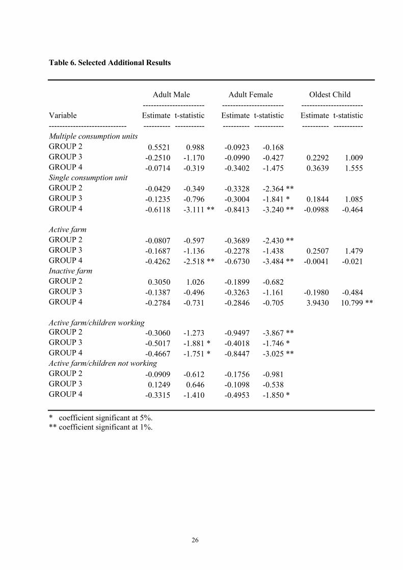
indicates whether the household includes more than one consumption unit. The results (table 6)
are strikingly supportive of the hypothesis that the effect of children is related to household
production considerations: the negative effects of the number of adult children on the parents�
tendency to work off the farm are statistically significant only when the children live with the
parents in the same house and do not maintain separate consumption units.14
Moving to the farm-related considerations, we first try to examine whether the number
of adult children matters more in active farms. We now interact the group dummies with a
dummy variable for active farms. The results (table 6) show that the negative effects of the
number of adult children on the parents� tendency to work off the farm are statistically
significant only in active farms.15 In addition, we interact the group dummies with a dummy
variable indicating whether at least one adult child is working on the farm. We use active farms
only, and because of the apparently high negative correlation between participation decisions on
farm and off the farm for the adult children, we drop the children�s equation and estimate a
bivariate probit model of the two parents only. The results (table 6) show that the negative
effects of the number of adult children on the parents� tendency to work off the farm are
statistically significant only in families with at at least one adult child who is working on the
farm. These last two results are clearly in support of the hypothesis that the effect of children is
related to farm production considerations as well.
Summary and Conclusions
This paper takes a deeper look at the phenomenon observed in previous research, that
the off-farm labor participation behavior of farm operators and their spouses depends on the
demographic composition of the household. Using data from a 1995 family farm survey, we
estimate jointly the off-farm participation equations of the farm operator, his or her spouse, and
their eldest adult child. We find that the number of adult children has a statistically significant
negative effect on the off-farm participation of farm couples, especially on that of the female.
An analysis of the predicted frequencies of off-farm labor participation revealed that for both
males and females, the variation across the groups of households defined by the number of adult
children is due in part to observed differences across the groups, and in part to genuine effects of
16
the number of adult children. We also find support to the hypothesis that this negative effect is
related to household production considerations as well as farm production considerations.
These conclusions contradict the results of previous research, but only under several
qualifications. First, previous research looked at the effects of the number of all adults in the
household, not only children, and included different forms of extended households, other than
the relatively simple households considered here. Second, the previous research looked at the
joint farm and off-farm labor participation decisions, while here we only examined off-farm
participation. Finally, it could be that the effects of household composition changed directions
and importance from 1981 to 1995. While all these qualifications could and will be studied in
future research, the last one is perhaps the most interesting and deserves more attention.
Another point that should be kept in mind for future research is that the number of adult
children living with the parents may be endogenous. It could be that adult children choose to
live with their parents on the farm in a way that depends on the parents� labor decisions. For
example, mothers who do not work off the farm are more available for child care services that
are demanded by the adult children. Prospects for farm succession could also play a role here.
As family history is not available in this data set, it is difficult to account for this possible
endogeneity. However, we expect to be able to match at least part of the sample with the 1981
data, and this may enable to trace, at least in part, children who left the family farm between the
two periods.
17
References
Ahituv, Avner, and Ayal Kimhi (forthcoming). �Off-Farm Work and Capital Accumulation
over the Farmer�s Life-Cycle.� Journal of Development Economics.
Becker, Gary S. (1991). A Treatise on the Family (Enlarged Edition). Cambridge: Harvard
University Press.
Blanc, Michel, and Philippe Perrier-Cornet (1993). "Farm Transfer and Farm Entry in the
EC." Sociologia Ruralis 33, 319-35.
Buttel, Fredrick H., and Gilbert W. Gillespie (1984). "The Sexual Division of Farm
Household Labor: An Exploratory Study of the Structure of On-Farm and Off-Farm Labor
Allocation among Farm Men and Women." Rural Sociology 49, 183-209.
Huffman, Wallace E. (1991). "Agricultural Household Models: Survey and Critique." In M.C.
Hallberg, J.L Findeis and D.A. Lass (eds.), Multiple Job-holding among Farm Families. Ames:
Iowa State University Press, 79-111.
Huffman, Wallace E., and Mark D. Lange (1989). "Off-Farm Work Decisions of Husbands
and Wives: Joint Decision Making." Review of Economics and Statistics LXXXI, 471-80.
Kimhi, Ayal (1994). "Quasi Maximum Likelihood Estimation of Multivariate Probit Models:
Farm Couples' Labor Participation." American Journal of Agricultural Economics 76, 828-835.
Kimhi, Ayal (1995). "Differential Human Capital Investments and the Choice of Successor in
Family Farms." American Journal of Agricultural Economics 77, 719-724.
Kimhi, Ayal (1996). "Demographic Composition of Farm Households and its Effect on Time
Allocation." Journal of Population Economics 9, 429-439.
Kimhi, Ayal (1998). �Institutional Environment, Ideological Commitment, and Farmers' Time
Allocation: the Case of Israeli Moshavim.� Economic Development and Cultural Change 47,
27-44.

18
Kimhi, Ayal, and Myoung-Jae Lee (1996). "Joint Farm and Off-Farm Work Decisions of
Farm Couples: Estimating Structural Simultaneous Equations with Ordered Categorical
Dependent Variables." American Journal of Agricultural Economics 78, 687-698.
Kimhi, Ayal, and Noga Nachlieli (2001). �Intergenerational Succession in Israeli Family
Farms.� Journal of Agricultural Economics 52, 42-58.
Lass, Daniel A., and Conrado M. Gempesaw (1992). "The Supply of Off-Farm Labor: A
Random Coefficients Approach." American Journal of Agricultural Economics 74, 400-11.
Shishko, Robert, and Bernard Rostker (1976). "The Economics of Multiple Job Holding."
American Economic Review 66, 298-308.
State of Israel, Central Bureau of Statistics (1998). Agricultural Survey 1995, Publication No.
1081, Jerusalem.
Sumner, Daniel A. (1982). "The Off-Farm Labor Supply of Farmers." American Journal of
Agricultural Economics 64, 499-509.
Tokle, J. G., and Wallace E. Huffman (1991). "Local Economic Conditions and Wage Labor
Decisions of Farm and Rural Nonfarm Couples." American Journal of Agricultural Economics
73, 652-70.
19
Table 1. Descriptive Statistics of Personal Variables
Variable All Group 1 Group 2 Group 3 Group 4
---------------------------------- ----------- ----------- ----------- ----------- ----------- Male Operator or Spouse WORKS ON FARM 0.68 0.63 0.70 0.75 0.79 WORKS OFF FARM 0.55 0.60 0.55 0.46 0.35 AGE 52.85 48.92 56.86 58.88 59.81 BORN IN ISRAEL 0.57 0.67 0.44 0.43 0.39 ASIA/AFRICA ORIGIN 0.23 0.28 0.19 0.18 0.07 HIGH SCHOOL 0.49 0.49 0.51 0.54 0.42 HIGHER EDUCATION 0.14 0.13 0.16 0.12 0.17 AGRICULTURAL EDUCATION 0.07 0.07 0.10 0.05 0.06
Female Operator or Spouse WORKS ON FARM 0.39 0.26 0.34 0.31 0.33 WORKS OFF FARM 0.46 0.51 0.44 0.45 0.24 AGE 48.79 44.78 52.46 55.00 56.41 BORN IN ISRAEL 0.60 0.70 0.52 0.45 0.42 ASIA/AFRICA ORIGIN 0.27 0.29 0.27 0.27 0.14 HIGH SCHOOL 0.48 0.49 0.48 0.47 0.43 HIGHER EDUCATION 0.13 0.14 0.13 0.11 0.13 AGRICULTURAL EDUCATION 0.05 0.05 0.04 0.05 0.07
Oldest Adult Child or Spouse WORKS ON FARM 0.24 0.23 0.22 0.29 WORKS OFF FARM 0.69 0.64 0.73 0.72 MALE 0.69 0.64 0.71 0.72 AGE 28.88 25.79 29.52 32.72 BORN IN ISRAEL 0.95 0.96 0.93 0.95 ASIA/AFRICA ORIGIN 0.39 0.41 0.36 0.42 HIGH SCHOOL 0.53 0.48 0.55 0.57 HIGHER EDUCATION 0.16 0.15 0.18 0.13 AGRICULTURAL EDUCATION 0.05 0.05 0.05 0.06
OBSERVATIONS 1949 1052 344 328 225
Note: off-farm work includes on-farm non-agricultural activities.
20
Table 2. Descriptive Statistics of Family, Operator, and Farm Variables
Variable All Group 1 Group 2 Group 3 Group 4
-------------------------- ----------- ----------- ----------- ----------- ----------- PRIVATE 0.08 0.09 0.08 0.07 0.03 ARAB 0.20 0.21 0.17 0.16 0.27 NORTH 0.29 0.29 0.36 0.26 0.27 SOUTH 0.24 0.27 0.23 0.16 0.18 ADOLESCENTS 0.80 0.75 1.03 0.90 0.64 CHILDREN 1.50 1.89 0.68 1.05 1.31 TENURE 28.50 26.10 28.99 33.14 34.42 SUCCEEDED 0.31 0.31 0.28 0.29 0.34 PURCHASED 0.28 0.31 0.27 0.22 0.19 SPECIALIZED 0.49 0.50 0.44 0.47 0.54 DIVERSIFIED 0.25 0.21 0.31 0.31 0.27 LAND 29.78 29.31 31.58 29.00 30.65 CAPITAL 99.58 89.94 101.39 123.22 116.34 FLOWERS 0.09 0.10 0.08 0.13 0.05 POULTRY 0.16 0.13 0.20 0.23 0.20 FIELD CROPS 0.27 0.24 0.28 0.28 0.39 CATTLE 0.08 0.09 0.06 0.06 0.08 OBSERVATIONS 1949 1052 344 328 225
21
Table 3. Quasi-Maximum Likelihood Estimation Results
Adult Male Adult Female Oldest Child ----------------------- ----------------------- -----------------------
Variable Estimate t-statistic Estimate t-statistic Estimate t-statistic ----------------------------- ---------- ----------- ---------- ----------- ---------- ----------- CORR. WITH FEMALE 0.2653 5.0970 ** CORR. WITH CHILD 0.2266 4.6850 ** 0.3797 6.6580 ** CONSTANT 0.1721 0.1640 -3.3368 -2.4980 ** -2.5188 -1.6090 GROUP 2 -0.0208 -0.1700 -0.3213 -2.3060 * 0.1770 1.1190 GROUP 3 -0.1616 -1.2060 -0.2471 -1.7150 * 0.0662 0.3550 GROUP 4 -0.3991 -2.5440 ** -0.5791 -3.1950 ** 0.3390 2.5100 ** AGE 0.0898 2.1850 * 0.2235 3.9220 ** 0.2065 2.1450 * AGE SQUARED -0.0013 -3.3420 ** -0.0027 -4.8460 ** -0.0030 -2.1230 * BORN IN ISRAEL 0.0136 0.1240 0.1973 1.9380 * 0.0005 0.0020 ASIA/AFRICA ORIGIN -0.0778 -0.7340 -0.0385 -0.3810 0.2846 1.8840 * HIGH SCHOOL 0.3633 3.4100 ** -0.0515 -0.4630 0.1132 0.7890 HIGHER EDUCATION 0.6395 4.7050 ** 0.0174 0.1230 -0.0472 -0.2390 AGRIC. EDUCATION -0.2571 -1.4450 0.0590 0.3240 -0.0717 -0.2860 NORTH 0.0976 0.8310 -0.2565 -2.1710 * -0.0939 -0.6100 SOUTH -0.3402 -2.6220 ** -0.3408 -2.5430 ** -0.0781 -0.4290 ADOLESCENTS 0.0442 0.9590 -0.0418 -0.7620 0.0311 0.4810 CHILDREN -0.0365 -1.5170 -0.0526 -1.6760 * -0.0233 -0.6180 TENURE 0.0001 0.0330 0.0015 0.3620 0.0015 0.3650 SUCCEEDED 0.0423 0.3030 0.0165 0.1230 0.2259 1.0330 PURCHASED 0.3100 2.5900 ** 0.0728 0.6130 0.3757 2.0400 * SPECIALIZED -0.7794 -5.2360 ** -0.1745 -1.2430 -0.3812 -1.5690 DIVERSIFIED -0.6913 -3.8140 ** 0.0750 0.4600 -0.4434 -1.6120 LAND 0.0034 1.6300 0.0075 3.7900 ** -0.0035 -1.1500 CAPITAL -0.0016 -4.9240 ** -0.0007 -2.7190 ** -0.0017 -5.0990 ** FLOWERS -0.5972 -4.4950 ** -0.2496 -1.7310 * -0.1628 -0.9750 POULTRY -0.3976 -2.9540 ** -0.4561 -3.2950 ** -0.1652 -0.9050 FIELD CROPS -0.6820 -6.0410 ** -0.4203 -3.5840 ** -0.1367 -0.9410 CATTLE -0.3846 -2.1180 * -0.1579 -0.7430 0.1687 0.7670 PRIVATE -0.4519 -2.5140 * -0.2401 -1.4530 -0.1001 -0.3860 ARAB -0.0932 -0.5310 -2.0098 -8.5100 ** -0.6444 -2.4970 **
* coefficient significant at 5%. ** coefficient significant at 1%

22
Table 4. Off-Farm Participation Results by Groups of Households
Group 1 Group 2 Groups 3-4 ----------------------- ----------------------- -----------------------
Variable Estimate t-statistic Estimate t-statistic Estimate t-statistic ----------------------------- ---------- ----------- ---------- ----------- ---------- ----------- CORR. MAL/FEM 0.2373 3.3540 ** 0.3749 3.4120 ** 0.2332 2.1770 * CORR. MAL/CHI 0.2392 1.9840 * 0.3814 3.6030 ** CORR. FEM/CHI 0.2315 1.9380 * 0.2729 2.6180 ** Male Operator or Spouse CONSTANT -0.0648 -0.0500 6.4253 1.3690 -11.8167 -2.5990 ** AGE 0.0924 1.7940 * -0.1296 -0.8330 0.5311 3.3770 ** AGE SQUARED -0.0013 -2.6200 ** 0.0005 0.4050 -0.0052 -3.8600 ** BORN IN ISRAEL -0.0673 -0.4620 0.1513 0.6030 0.0201 0.0900 ASIA/AFRICA ORIGIN 0.0048 0.0350 -0.3206 -1.2620 0.0530 0.2100 HIGH SCHOOL 0.2952 2.0780 * 0.5562 2.2200 * 0.3735 1.7430 * HIGHER EDUCATION 0.8062 4.3030 ** 0.4722 1.5680 0.5292 1.8780 * AGRIC. EDUCATION 0.0400 0.1530 -0.6227 -1.9220 * -0.8651 -2.3960 ** NORTH 0.2657 1.5830 -0.2232 -0.8970 0.0109 0.0450 SOUTH -0.1670 -0.9240 -1.0321 -3.7140 ** -0.2203 -0.8910 ADOLESCENTS 0.0351 0.5640 0.2101 2.1800 * 0.0343 0.3660 CHILDREN -0.0354 -1.1570 -0.1351 -1.3950 -0.0274 -0.4580 TENURE -0.0012 -0.3740 0.0081 1.0380 -0.0037 -0.6270 SUCCEEDED 0.0696 0.3700 -0.0676 -0.1930 0.2765 1.0780 PURCHASED 0.4106 2.6070 ** 0.2952 1.0610 0.2316 0.9150 SPECIALIZED -0.6853 -3.3950 ** -1.1115 -3.2960 ** -1.0198 -3.3120 ** DIVERSIFIED -0.7431 -3.1720 ** -0.5110 -1.2610 -0.8297 -2.1370 * LAND 0.0023 0.8020 0.0215 3.8610 ** -0.0046 -1.0340 CAPITAL -0.0018 -4.6950 ** -0.0019 -3.0170 ** -0.0013 -2.0220 * FLOWERS -0.6591 -3.9510 ** -1.0171 -3.3110 ** -0.1633 -0.6160 POULTRY -0.3314 -1.7190 * -0.7211 -2.3270 ** -0.3870 -1.4140 FIELD CROPS -0.6866 -4.4180 ** -1.5880 -6.0310 ** -0.3902 -1.7310 * CATTLE -0.4392 -1.8090 * -0.4089 -1.0040 -0.4731 -1.1800 PRIVATE -0.4830 -1.9090 * -1.0747 -2.7100 ** 0.0719 0.1740 ARAB 0.0519 0.2300 0.2647 0.5680 -0.5307 -1.4370 GROUP 4 -0.1669 -0.8850
Continued on next page

23
Table 4. (continued)
Group 1 Group 2 Groups 3-4 ----------------------- ----------------------- -----------------------
Variable Estimate t-statistic Estimate t-statistic Estimate t-statistic ----------------------------- ---------- ----------- ---------- ----------- ---------- ----------- Female Operator or Spouse CONSTANT -3.2078 -2.2870 * -21.5404 -3.5940 ** -15.2294 -2.6450 ** AGE 0.2068 3.3010 ** 0.8940 3.9790 ** 0.6737 3.1480 ** AGE SQUARED -0.0026 -4.0290 ** -0.0088 -4.2070 ** -0.0069 -3.4570 ** BORN IN ISRAEL 0.1615 1.1590 0.1840 0.7010 0.4381 2.0050 * ASIA/AFRICA ORIGIN -0.0847 -0.6350 -0.1250 -0.5240 0.2529 1.1550 HIGH SCHOOL 0.0228 0.1530 0.1317 0.4760 -0.4156 -1.8180 * HIGHER EDUCATION -0.1131 -0.6000 0.5009 1.4530 -0.2292 -0.7700 AGRIC. EDUCATION 0.3942 1.6220 0.1429 0.3130 -0.5191 -1.5510 NORTH -0.2262 -1.4650 0.0165 0.0560 -0.7171 -2.9290 ** SOUTH -0.1705 -0.9540 -0.8114 -2.6050 ** -0.5932 -2.0920 * ADOLESCENTS 0.0190 0.2670 0.0213 0.1760 -0.2378 -1.8980 * CHILDREN -0.0636 -1.5100 0.1656 1.8230 * -0.0304 -0.5030 TENURE 0.0061 1.2560 -0.0091 -1.2580 -0.0063 -0.7610 SUCCEEDED 0.0943 0.5480 -0.6563 -1.9460 * 0.0089 0.0320 PURCHASED 0.1958 1.2560 -0.4618 -1.5690 -0.0568 -0.2320 SPECIALIZED -0.2773 -1.5330 -0.3146 -0.8790 0.2812 0.9290 DIVERSIFIED 0.1155 0.5390 0.0208 0.0490 0.1688 0.5130 LAND 0.0069 2.7860 ** 0.0108 2.1560 * 0.0164 3.8080 ** CAPITAL -0.0008 -2.4720 ** -0.0001 -0.1140 -0.0016 -2.8860 ** FLOWERS -0.1286 -0.6960 -0.8675 -3.1400 ** -0.4040 -1.4410 POULTRY -0.2491 -1.3350 -1.0459 -3.0030 ** -0.6429 -2.3700 ** FIELD CROPS -0.3046 -1.9480 * -0.8033 -2.9380 ** -0.6411 -2.6400 ** CATTLE -0.1393 -0.4210 0.3797 0.7960 -0.5049 -1.3660 PRIVATE -0.0144 -0.0640 -0.0005 -0.0010 -1.2088 -2.5980 ** ARAB -2.3819 -9.2190 ** -1.4724 -2.7250 ** -2.2574 -4.5600 ** GROUP 4 -0.4698 -2.3070 *
Continued on next page

24
Table 4. (continued)
Group 1 Group 2 Groups 3-4 ----------------------- ----------------------- -----------------------
Variable Estimate t-statistic Estimate t-statistic Estimate t-statistic ----------------------------- ---------- ----------- ---------- ----------- ---------- ----------- Oldest Adult Child or Spouse CONSTANT -2.5711 -1.0520 -3.3091 -1.4990 MALE 0.1789 0.7990 0.4098 2.3570 ** AGE 0.1976 1.3410 0.2637 1.9490 * AGE SQUARED -0.0030 -1.3280 -0.0037 -1.8910 * BORN IN ISRAEL 0.4261 0.9250 -0.1246 -0.3420 ASIA/AFRICA ORIGIN 0.5250 1.9080 * 0.1929 1.0370 HIGH SCHOOL 0.2139 0.8960 0.0488 0.2690 HIGHER EDUCATION -0.0105 -0.0320 -0.0950 -0.3690 AGRIC. EDUCATION -0.3896 -0.8790 0.0094 0.0310 NORTH -0.0536 -0.2030 -0.1794 -0.8920 SOUTH -0.0689 -0.2140 -0.1556 -0.6910 ADOLESCENTS 0.0285 0.2700 0.0550 0.6210 CHILDREN -0.0962 -1.0620 -0.0205 -0.4810 TENURE 0.0008 0.1210 0.0017 0.3370 SUCCEEDED 0.0639 0.1690 0.3888 1.4810 PURCHASED 0.0037 0.0120 0.7188 3.1800 ** SPECIALIZED -0.6171 -1.6240 * -0.1654 -0.4930 DIVERSIFIED -0.4650 -1.0510 -0.4228 -1.1210 LAND -0.0019 -0.3390 -0.0040 -1.0170 CAPITAL -0.0012 -2.1190 * -0.0021 -4.4610 ** FLOWERS -0.4133 -1.4950 -0.1402 -0.6330 POULTRY -0.5100 -1.4990 -0.0683 -0.3010 FIELD CROPS 0.0455 0.1780 -0.2946 -1.5720 CATTLE 0.1194 0.2930 0.2529 0.9420 PRIVATE 0.0261 0.0700 -0.4836 -1.3970 ARAB -0.4018 -0.9070 -0.8511 -2.6350 ** GROUP 4 -0.1424 -0.8230
* coefficient significant at 5%. ** coefficient significant at 1%.
25
Table 5. Comparing Actual and Predicted Off-Farm Participation Frequencies
Group of Households ----------------------------------------------- 1 2 3 4 All ---------- ---------- ---------- ---------- ----------
Males Actual frequency 0.602 0.553 0.456 0.354 0.547 Joint estimation Predicted 0.674 0.624 0.433 0.324 0.593 At the means 0.483 0.475 0.419 0.330 0.453 Separate estimation Predicted 0.657 0.582 0.464 0.321 At the means 0.426 0.468 0.293 0.238
Females Actual frequency 0.510 0.441 0.451 0.240 0.463 Joint estimation Predicted 0.659 0.517 0.502 0.186 0.563 At the means 0.486 0.361 0.389 0.269 0.421 Separate estimation Predicted 0.638 0.474 0.460 0.220 At the means 0.420 0.183 0.207 0.099
Children Actual frequency 0.641 0.725 0.715 0.691 Joint estimation Predicted 0.797 0.896 0.842 0.844 At the means 0.610 0.676 0.635 0.640 Separate estimation Predicted 0.811 0.860 0.787 At the means 0.605 0.657 0.604
Note: the actual frequencies are somewhat different from those reported in table 1 because of the different treatment of missing values.
26
Table 6. Selected Additional Results
Adult Male Adult Female Oldest Child ----------------------- ----------------------- -----------------------
Variable Estimate t-statistic Estimate t-statistic Estimate t-statistic ----------------------------- ---------- ----------- ---------- ----------- ---------- ----------- Multiple consumption units GROUP 2 0.5521 0.988 -0.0923 -0.168 GROUP 3 -0.2510 -1.170 -0.0990 -0.427 0.2292 1.009 GROUP 4 -0.0714 -0.319 -0.3402 -1.475 0.3639 1.555 Single consumption unit GROUP 2 -0.0429 -0.349 -0.3328 -2.364 ** GROUP 3 -0.1235 -0.796 -0.3004 -1.841 * 0.1844 1.085 GROUP 4 -0.6118 -3.111 ** -0.8413 -3.240 ** -0.0988 -0.464 Active farm GROUP 2 -0.0807 -0.597 -0.3689 -2.430 ** GROUP 3 -0.1687 -1.136 -0.2278 -1.438 0.2507 1.479 GROUP 4 -0.4262 -2.518 ** -0.6730 -3.484 ** -0.0041 -0.021 Inactive farm GROUP 2 0.3050 1.026 -0.1899 -0.682 GROUP 3 -0.1387 -0.496 -0.3263 -1.161 -0.1980 -0.484 GROUP 4 -0.2784 -0.731 -0.2846 -0.705 3.9430 10.799 ** Active farm/children working GROUP 2 -0.3060 -1.273 -0.9497 -3.867 ** GROUP 3 -0.5017 -1.881 * -0.4018 -1.746 * GROUP 4 -0.4667 -1.751 * -0.8447 -3.025 ** Active farm/children not working GROUP 2 -0.0909 -0.612 -0.1756 -0.981 GROUP 3 0.1249 0.646 -0.1098 -0.538 GROUP 4 -0.3315 -1.410 -0.4953 -1.850 *
* coefficient significant at 5%. ** coefficient significant at 1%.
27
Notes 1 Kimhi (1998) provides a detailed description of the historical institutional structure of Moshavim. However, by 1995 most Moshavim had very little cooperation left. 2 It is important to note that the number of adult children include only those who are currently residing on the farm, either as part of the parents� household or as a separate �succeeding� household, hence it has nothing to do with the number of children the parents ever had. 3 Value added is �normative�, meaning that it was calculated using weights attached to physical measures of production, such as size of crop areas and number of animals. 4 This could be larger or smaller to the size of land that is actually operated. This variable could easily be thought of as exogenous or at least predetermined (Kimhi 1998). 5 The use of capital stock as an explanatory variable could be problematic, due to possible endogeneity (Ahituv and Kimhi, forthcoming). 6 Although a farm could have production in more than one branch, we exclude the dummy for fruits in order to avoid collinearity with the specialization dummies through the inactive farms. 7 We do not show the statistics for adult children other than the oldest, since they will not be included in the estimated model, as will be explained below. 8 Farm succession in Moshavim has the incentive of obtaining a permit to build another house on the farm, while this is not necessarily the case in private family farms (Kimhi and Nachlieli 2001). 9 On the other hand, group 1 can include elderly households in which children have grown up and left. 10 The code is available from the corresponding author upon request. 11 It should be emphasized that when data were missing for an individual we excluded that individual only, not the whole household. 12 To test these two explanations, a panel data set with at least three periods is necessary (Ahituv and Kimhi, forthcoming). 13 These results are available from the corresponding author upon request. 14 We only list the coefficients of the group dummies. Full results are available from the corresponding author upon request. 15 The large and significant coefficient of group 4 in the sample of inactive farms is because of the small number of observations in that category and should not be interpreted as is.