TitleExtrema of logarithmically correlated random field: Knownand new results (Stochastic Analysis on Large Scale InteractingSystems)
Author(s) Abe, Yoshihiro
Citation 数理解析研究所講究録別冊 = RIMS Kokyuroku Bessatsu(2016), B59: 117-128
Issue Date 2016-07
URL http://hdl.handle.net/2433/243597
Right © 2016 by the Research Institute for Mathematical Sciences,Kyoto University. All rights reserved.
Type Departmental Bulletin Paper
Textversion publisher
Kyoto University

RIMS Kôkyûroku BessatsuB59 (2016), 117−128
Extrema of logarithmically correlated random field:Known and new results
By
Yoshihiro ABE*
Abstract
In this paper, we have two main purposes. Firstly, we describe known results on extrema oflogarithmically correlated random fields such as the branching Brownian motion, the branchingrandom walk, the two‐dimensional discrete Gaussian free field, and cover times of the two‐dimensional torus and the binary tree. Secondly, we announce a new result on extrema of localtimes for the simple random walk on the b‐ary tree.
§1. Introduction
Logarithmically correlated random fields have been studied extensively since they
appear naturally in relation to a number of different mathematical problems, some 0
which are mentioned below. There are several properties which are common to all such
fields, and which are different from those of independent and identically distributed
random variables. We will focus our attention to the branching Brownian motion, the
branching random walk, the two‐dimensional discrete Gaussian free field, and cover
times for the two‐dimensional torus and the binary tree. These models have fruitful
connections with many subjects: partial differential equations (the Fisher‐KPP equa‐tion) [21], spin glasses [19, 20], random multiplicative cascade measures [36], the theoryof fixed points of smoothing transforms [33], the two‐dimensional Liouville quantumgravity [32, 14].
We recently studied extrema of local times for the simple random walk on the b‐ary
tree [1]. Thanks to the Dynkin isomorphism [34, 35], the local times are closely related
Received January 30, 2016. Revised May 2, 2016.2010 Mathematics Subject Classification(s): 60J55, 60G70, 60G57
Ke Words: Local time, Branching random walk, Branching Brownian motion, Discrete Gaussiafree field.Supported by JSPS KAKENHI 13J01411
*
Graduate School of Science, Kobe University, Rokkodai‐cho 1‐1, Nada‐ku, Kobe, 657‐8501, Japan. e‐mail: yosihiro@math. kobe -u . ac. jp
© 2016 Research Institute for Mathematical Sciences, Kyoto University. All rights reserved.

118 Yoshihiro Abe
to the branching random walk, and exploring explicit connections between the two is
the main motivation of the study.
In Section 2, we describe known results on logarithmically correlated random mod‐
els. In Section 3, we announce a new result on local times for the simple random walk
on the b‐ary tree.
We give some notation which we use throughout the paper. Given functions f and
g , we will write f(x)\sim g(x) as xarrow 1 if \lim_{xarrow\infty}f(x)/g(x)=1 . For random variables X and Y, \backslash \backslash X^{1aw}=Y ” means that the law of X is the same as that of Y . We will write
\delta_{p} to denote the Dirac measure at a point p . Fix a complete, separable metric space
X. Let M_{+}(\mathcal{X}) be the set of all non‐negative Radon measures on \mathcal{X} topologized with
the vague topology. Since M_{+}(\mathcal{X}) is metrizable as a complete, separable metric space,
we can consider convergence in law of random elements of M_{+}(\mathcal{X}) . Given a sequence o
random measures (\mu_{n})_{n\geq 1} and a random element \mu in M_{+}(\mathcal{X}) , we will write \backslash \backslash \mu_{n} law \mu
in M_{+}(\mathcal{X}) ” as narrow 1 if for any continuous, non‐negative function f on \mathcal{X} with compact
support, \int_{\mathcal{X}}fd\mu_{n} weakly converges to \int_{\mathcal{X}}fd\mu as narrow 1 . Given a random element vo
M_{+}(\mathcal{X}) , we will write PPP (v) to denote a point process on \mathcal{X} which, conditioned on v,
is the Poisson point process on \mathcal{X} with intensity measure v (that is, PPP(v) is a Coxprocess).
§2. Logarithmically correlated random fields
In this section, we describe known results on some logarithmically correlated ran‐
dom fields. We refer to [37] for a general description of this topic.
§2.1. Branching Brownian motion
In this subsection, we collect known results on extrema of the branching Brownian
motion (BBM . We refer to [17] for an overview of BBM. BBM is a probabilistic modeldescribing the growth of population of particles moving in a space. This model is
defined as follows: At time 0 , a particle starts at the origin and behaves like a standardBrownian motion on \mathbb{R} up to time T which is distributed as an exponential distribution
with mean 1 and independent of the Brownian motion. Let a be the position of the
particle at time T . At time T , the particle splits into two particles. Independently, eachof the particles starts at a and performs a standard Brownian motion on \mathbb{R} up to an
exponential time of parameter 1 and splits into two particles. Repeating this procedure,
we obtain a BBM. Let x_{1}(t) , :::, x_{n(t)}(t) be positions of the particles at time t . One
of the striking features of the BBM is that the maximum of the BBM is related to
a reaction‐diffusion equation called the Fisher equation or the Kolmogorov‐Petrovsky‐
Piscounov (KPP) equation: McKean [41] proved that the law of the maximum of the
Extrema of logarithmically correlated random FiELD: Known and new results 119
BBM u(t, x) :=\mathbb{P} (max1 \leq i\leq n(t)^{X_{i}(t)} \leq x ) is the solution 0
\frac{\partial u}{\partial t} = \frac{1}{2}\frac{\partial^{2}u}{\partial x^{2}}+u^{2}-u, u(0, x)=1_{\{x\geq 0\}}.Lalley and Sellke [38] showed that there exists a positive constant \alpha_{bbm} such that forall x\in \mathbb{R},
(2.1) \lim_{tarrow\infty}\mathbb{P}(_{1}\max_{\leq i\leq n(t)}x_{i}(t) \leq m_{t}^{bbm}+x) =E[\exp\{-\alpha_{bbm}Z_{bbm}e^{-} 2x\}] ,
where
m_{t}^{bbm}:= 2t- \frac{3}{22}\log t,and Z_{bbm} is the limit of the so‐called derivative martingale:
n(t)
(2.2) Z_{bbm} :=t \lim \sum_{i=1}( 2t-x_{i}(t))e^{-} 2( 2t-x_{i}(t)) .
(It is known that the limit on the right of (2.2) exists almost surely.) Thus, the limitlaw of the maximum of BBM is a Gumbel distribution with a random mean given by
the derivative martingale. The derivative martingale is essentially determined by the
positions of the particles at time o(t) and conditionally on these positions, particles
behave independently, which explains the appearance of the Gumbel distribution. Let
\omega_{bbm}(x) be the right of (2.1). It is known that
(2.3) 1-\omega_{bbm}(x)\sim\alpha_{bbm}xe^{-} 2x
as xarrow 1.
In [4, 5], Arguin, Bovier, and Kistler showed that the first branching time for any twoextremal particles at time t is either less than r or larger than t-r with probability
tending to 1 as t arrow 1 and then r arrow 1 , and that a point process encoding local
extrema of positions of the particles converges to a Cox process. The convergence 0
the full extremal process of the BBM has been settled by [3, 6]: they proved that thereexist independent and identically distributed point processes \mathcal{D}^{(i)} := \sum_{j\geq 1}\delta_{d_{j}^{(i)}}, i \in \mathbb{N}
such that as tarrow 1,
(2.4) \sum_{i=1}^{n(t)}\delta_{x_{i}(t)-m_{t}^{bbm}} law \sum_{i}\delta_{x_{i}+d_{j}^{(i)}} in M_{+}(\mathbb{R}) ,
where x_{i}, i\in \mathbb{N} are atoms of the Cox process PPP (\alpha_{bbm}Z_{bbm} 2e^{-} 2xdx) . We empha‐
size that the authors of [3, 6] gave an explicit description of the decoration point process \mathcal{D}^{(1)} . Recently, adding information about the “location” of particles in the genealogy
tree, Bovier and Hartung [18] extended the convergence of the extremal process. We

120 Yoshihiro Abe
stress that the above results have been established for BBM with more general branchingbehaviour.
§2.2. Branching random walk
In this subsection, we describe known results on extrema of the branching random
walk (BRW) and random multiplicative cascade measures. We refer to [42] for theformer and to [9] and references therein for the latter. To simplify the description, weonly consider a very simple version of the BRW: Consider the binary tree T with a
distinguished point \rho called root. This is a graph with the vertex set T= \bigcup_{k\geq 0}T_{k} and
the edge set E(T) := \{\{\rho, v\} : v\in T_{1}\}\cup\bigcup_{k\geq 1}\{\{v, vu\} : v\in T_{k}, u\in T_{1}\} , where
T_{0} :=\{\rho\}, T_{k} :=\{(V_{1}, \ldots, V_{k}) : V_{i}\in\{0, 1\}, 1\leq i\leq k\}, k\geq 1,
and for v=(V_{1}, \ldots, V_{k}) \in T_{k} and u=(u_{1}, \ldots, \overline{u}_{\ell}) \in T_{\ell} , we set
vu := ( v_{1}, \ldots, v_{k} , u1, :::, \overline{u}_{\ell} ).
Let (Y_{e})_{e\in E(T)} be a family of independent standard normal random variables. To each
v\in T_{k}, k\geq 1 , we assign
h_{v} := \sum_{i=1}^{k}Y_{e_{i}^{v}},where e_{1}^{v} , :::, e_{k}^{v} are the edges on the unique path from \rho to v . We will call (h_{v}^{T})_{v\in T} a
BRW on T.
2.2.1. Extrema of the branching random walk
Due to [7, 2, 25], it is known that there exists a positive constant \alpha_{brw} such thatfor all \lambda\in \mathbb{R},
(2.5) \lim_{narrow\infty}\mathbb{P}(\max_{v\in T_{n}}\frac{1}{2}h_{v} \leq m_{n}^{brw}+\lambda) =E[\exp\{-\alpha_{brw}Z_{brw}e^{-2\sqrt{\log 2}\lambda}\}] ,
where
(2.6) m_{n}^{brw} := \log 2n-\frac{3}{4\log 2}\log n,and Z_{brw} is the limit of the deri \sqrt{}ative martingale:
(2.7) Z_{brw}:= \lim_{n} \sum_{v\in T_{n}} ( \log 2n-\frac{1}{2}h_{v})e^{-2\sqrt{\log2}(\sqrt{\log 2}n-\frac{1}{2}h_{v})}.(It is known that the limit on the right of (2.7) exists almost surely.) Let \omega_{brw}(\lambda) bethe right of (2.5). It is known (see [2, Proposition 1.3] or [25, Proposition 3.1]) that
(2.8) 1 — \omega_{brw}(\lambda)\sim\alpha_{brw}\lambda e^{-2\sqrt{102}\lambda} as \lambdaarrow 1.
Extrema of logarithmically correlated random FiELD: Known and new results 121
We emphasize that Bachmann [7], A^{\cdot}idékon [2], and Bramson, Ding, and Zeitouni [25] ob‐tained results corresponding to (2.5) for more general branching random walks. Madaule[40] established the convergence of the full extremal process of the BRW similar to (2.4).
2.2.2. Random multiplicative cascade measures
Random multiplicative cascade measures (we will call cascade measures, for short)were introduced by Mandelbrot in the study of turbulence. According to a positive
parameter \beta corresponding to the inverse temperature, cascade measures fall into three
types: subcritical (\beta < 1) , critical (\beta = 1) , and supercritical (\beta > 1) . To define the
cascade measures, we give some notation. Let
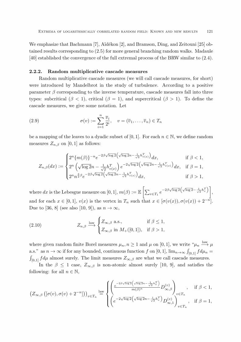
(2.9) \sigma(v) := \sum_{i=1}^{n}\frac{\overline{v}_{i}}{2^{i}}, v= (v1, :::, \overline{v}_{n} ) \in T_{n}
be a mapping of the leaves to a dyadic subset of [0 , 1 ] . For each n\in \mathbb{N} , we define random
measures Z_{n,\beta} on [0 , 1 ] as follows:
Z_{n,\beta} (dx) := \{\begin{array}{ll}2^{n}\{m(\beta)\}^{-n}e^{-2\beta\sqrt{102}(\sqrt{102}n-\frac{1}{2}h_{vx})}dx, if \beta<1,2^{n}(\sqrt{\log 2}n-\frac{1}{2}h_{v(x)})e^{-2\sqrt{\log}(\sqrt{\log 2}n-\frac{1}{2}h_{vx}})_{dx}, if \beta=1,2^{n}n^{\frac{3}{2}\beta}e^{-2\beta\sqrt{\log 2}(\sqrt{\log 2}n-\frac{1}{2}h_{vx}})_{dx}, if \beta>1,\end{array}where dx is the Lebesgue measure on [0 , 1 ], m(\beta) :=E [ \sum_{v\in T_{1}}e^{-2\beta\sqrt{102}(\sqrt{102}-\frac{1}{2}h_{v}})],and for each x\in [0 , 1 ], v(x) is the vertex in T_{n} such that x\in [\sigma(v(x)), \sigma(v(x))+2^{-n}].Due to [36, 8] (see also [10, 9]), as narrow 1,
(2.10) Z_{n,\beta} law \{\begin{array}{ll}Z_{\infty,\beta} a.s., if \beta\leq 1,Z_{\infty,\beta} in M_{+}([0,1]) , if \beta> 1,\end{array}where given random finite Borel measures \mu_{n}, n\geq 1 and \mu on [0 , 1 ] , we write \backslash \backslash \mu_{n} law \mu
a.s.” as narrow 1 if for any bounded, continuous function f on [0 , 1 ], \lim_{narrow\infty}\int_{[0,1]}fd\mu_{n}= \int_{[0,1]}fd\mu almost surely. The limit measures Z_{\infty,\beta} are what we call cascade measures.
In the \beta \leq 1 case, Z_{\infty,\beta} is non‐atomic almost surely [10, 9], and satisfies thefollowing: for all n\in \mathbb{N},
(Z_{\infty,\beta} ([\sigma(v), \sigma(v) +2^{-n}]))_{v\in T_{n}} 1aw= \{\begin{array}{ll}(\frac{e^{-2\beta\sqrt{\log 2}(\sqrt{\log 2}n-\frac{1}{2}h_{v})}}{m(\beta)^{n}}D_{\infty,\beta}^{(v)})_{v\in T_{n}}, if \beta< 1,(e^{-2\sqrt{\log 2}(\sqrt{\log 2}n-\frac{1}{2}h_{v}})_{D_{\infty,1}^{(v)})_{v\inT_{n}}}, if \beta=1,\end{array}

122 Yoshihiro Abe
where D^{(v)} \infty,\beta, v\in T_{n} are indepesdent copies of Z_{\infty,\beta}([0,1]) . In particular, we have
(2.11) Z_{\infty,\beta}([0,1])^{1aw}= \{\begin{array}{ll}\sum_{v\in T_{1}} \frac{e^{-2\beta\sqrt{\log 2}(\sqrt{\log 2}-\frac{1}{2}h_{v})}}{m(\beta)}D_{\infty,\beta}^{(v)}, if \beta< 1,\sum_{v\in T_{1}}e^{-2\sqrt{\log 2}(\sqrt{\log 2}-\frac{1}{2}h_{v}})_{D_{\infty,1}^{(v)}}, if \beta=1.\end{array}Due to, for example, [12, Theorem 3], Z_{\infty,\beta}([0,1]) is the unique solution of the distri‐butional equation (2.11) (called the fixed point of the smoothing transform) up to amultiplicative constant in the space of non‐trivial finite non‐negative random variables.
Tails of Z_{\infty,\beta}([0,1]) are well studied. See, for example, [39, 26].In the \beta> 1 case, Barral, Rhodes, and Vargas [8] showed that there exists a positive
constant c(\beta) such that
Z_{\infty,\beta}=c(\beta)T_{\frac{1}{\beta}}(Z_{\infty,1})1aw,where T_{\frac{1}{\beta}} is a subordinator with the Laplace transform
E[e^{-\lambda T_{\frac{1}{\beta}}(t)}] =e^{-t\lambda^{\frac{1}{\beta}}}, t\geq 0, \lambda\geq 0,and T_{\frac{1}{\beta}}(Z_{\infty,1}) is a random Borel measure on [0 , 1 ] which satisfies
T_{\frac{1}{\beta}}(Z_{\infty,1})((a, b])=T_{\frac{1}{\beta}}(Z_{\infty,1}([0, b]))-T_{\frac{1}{\beta}}(Z_{\infty,1}([0, a])) , 0\leq a<b\leq 1,where T_{\frac{1}{\beta}} is independent of Z_{\infty,1} . In particular, Z_{n,\beta} is atomic almost surely if \beta> 1.
One of the remarkable features of cascade measures is the so‐called KPZ formula
proved by Benjamini and Schramm [10] in the \beta < 1 case and Barral et a1.[9] in the \beta = 1 case: Fix \beta \leq 1 and a deterministic, nonempty Borel set K \subset [0 , 1 ] . Let \xi_{0} (\xi,respectively) be the Hausdorff dimension of K with respect to the Euclidean metric (withrespect to the random metric d_{\beta} defined by d_{\beta}(x, y) := Z_{\infty,\beta}([x, y]) , 0 \leq x \leq y \leq 1,
respectively). Then, the following holds almost surely:
\xi_{0}-\xi=\beta^{2}\xi(1-\xi) .
We note that the above results hold in more general settings.
§2.3. Two‐dimensional discrete Gaussian free field
In this subsection, we collect known results on extrema of the two‐dimensional
discrete Gaussian free field (DGFF). We refer to [42] for an overview of this model. Set V_{n} := [0, n]^{2}\cap \mathbb{Z}^{2} . Let \partial V_{n} be the inner vertex boundary of V_{n} . The two‐dimensional
DGFF is a family of centered Gaussian random variables h^{V_{n}} = \{h_{x}^{V_{n}} : x \in V_{n}\} withcovariance
E[h_{x}^{V_{n}}h^{V_{n}}] =E_{x} [\sum_{i=0}^{H_{\partial V_{n}}-1}1_{\{S_{i}=y\}}] ,

Extrema of logarithmically correlated random FiELD: Known and new results 123
where S = (S_{i}, i \geq 0, P_{x}, x \in V_{n}) is the discrete‐time simple random walk on V_{n} and
H_{A} is the hitting time of a subset A\subset V_{n} by S . Thanks to the so‐called Gibbs‐Markov
property of h^{V_{n}} , the DGFF can be approximated by a BRW. This elegant idea goes
back to [15], and was revisited by [16, 23]. Bramson, Ding, and Zeitouni [24] provedthat there exist a positive constant \alpha ff and an almost surely positive random variable
Z_{gff} such that for all \lambda\in \mathbb{R},
(2.12) \lim_{narrow\infty}\mathbb{P}(\max_{x\in V_{n}}h_{x}^{V_{n}} \leq m_{n}^{g} +\lambda) =E[\exp\{-\alpha_{gff}Z_{gff}e^{-\sqrt{2\pi}\lambda}\}] ,
where
m_{n}^{g} :=2 \frac{2}{\pi}\log n-\frac{3}{4} \frac{2}{\pi}\log(\log n) .
Let \omega_{gff}(\lambda) be the right of (2.12). It is known (see [24, Proposition 4.1]) that
(2.13) 1-\omega_{gff}(\lambda) \sim\alpha_{gff}\lambda e^{-\sqrt{2\pi}\lambda} as \lambdaarrow 1.
Ding and Zeitouni [31] studied the geometry of the set of vertices with values close to m_{n}^{gff} . Biskup and Louidor [13] considered the point process on [0 , 1 ]^{2} \cross \mathbb{R}
\eta_{n,r}:=\sum_{x\in V_{n}}\delta_{(\frac{x}{n},h_{x}^{V_{n}}-m_{n}^{gff})}1_{\{h_{x}^{V_{n}}=\max_{y\in\Lambda_{r}(x)}h_{y^{n}}^{V}\}}, r>0, n\in \mathbb{N},where \Lambda_{r}(x) := \{y \in \mathbb{Z}^{2} : |y - x|_{1} \leq r\} and showed that there exists a random
Borel measure Z_{\infty}^{gff} on [0 , 1 ]^{} such that for any (r_{n})_{n\geq 1} with \lim_{narrow\infty}r_{n} = 1 and
\lim_{narrow\infty}r_{n}/n=0 , as narrow 1,
(2.14) \eta_{n,r_{n}} law PPP (Z^{gff}(dx)\otimes e^{-\sqrt{2\pi}h}dh) in M_{+}([0,1]^{2} \cross \mathbb{R})They investigated properties of the limiting measure Z^{gff} and revealed that it is a version
of the derivative martingale associated with the continuum Gaussian free field. In [14],they discuss a possible connection between extrema of the DGFF and the so‐called
critical Liouville quantum gravity.
§2.4. Cover times
In this subsection, we describe results on cover times for the planar Brownian
motion by Belius and Kistler [11] and the simple random walk on the binary tree dueto Ding and Zeitouni [30].
2.4.1. Cover time for the planar Brownian motionConsider the two‐dimensional torus \mathbb{T} :=(\mathbb{R}/\mathbb{Z})^{2} . Let B(x, r) be the closed ball 0
radius r in \mathbb{T} centered at x . For \epsilon>0 , we define the \epsilon‐cover time by
C_{\varepsilon} := \sup_{x\in \mathbb{T}}H_{B(x,\varepsilon)},

124 Yoshihiro Abe
where H_{A} is the hitting time of a subset A \subset \mathbb{T} by the standard Brownian motion on
T. Let P_{x} be the law of the Brownian motion started at x\in \mathbb{T} . Belius and Kistler [11]studied the \epsilon‐cover time by analyzing the number of crossings of consecutive annuli by
the Brownian motion (“traversal process in their word) which enabled them to applytechniques developed in the study of the BBM. A key of the relation with the BBM
is a hierarchical structure of the traversal process (see [11, Figure 6.1]) and this ideagoes back to [27, 28]. Belius and Kistler [11] proved that for all \delta > 0 and x \in \mathbb{T} , thefollowing holds with P_{x} ‐probability tending to 1 as \epsilonarrow 0 :
2 \log\epsilon^{-1}-(1+\delta)\log(\log\epsilon^{-1}) \leq \frac{C_{\varepsilon}}{\frac{1}{\pi}\log\epsilon^{-1}} \leq 2\log\epsilon^{-1}-(1-\delta)\log(\log\epsilon^{-1}) .
Further properties such as the tightness and convergence in law are still unknown.
2.4.2. Cover time for the simple random walk on the binary tree
Recall the notation in Section 2.2. Let T_{\leq n} be the binary tree of depth n given by
T_{\leq n}:= \bigcup_{k=0}^{n}T_{k}.
We define the cover time for the simple random walk on T_{\leq n} by
\tau_{cov}^{n}:=\max_{v\in T_{\leq n}}H_{v},where H_{v} is the hitting time of v by the simple random walk on T_{\leq n} started at the
root. Ding and Zeitouni [30] showed that there exist positive constants c_{1}, c_{2} \in (0, \infty)such that the following holds with probability tending to 1 as narrow\infty :
(2.15)
\sqrt{2\log 2}n-\frac{\log n}{\sqrt{2\log 2}}-c_{1}(\log(\log n))^{8}\leq \sqrt{\frac{\tau_{cov}^{n}}{|E_{n}|}}\leq \sqrt{2\log 2}n-\frac{\log n}{\sqrt{2\log 2}}+c_{2}(\log(\log n))^{8},where |E_{n}| is the total number of edges in T_{\leq n} . A key step of the proof is comparison
between densities of local times and Gaussian random variables [30, Lemma 2.7]. Bram‐son and Zeitouni [22, Theorem 1.2] established a tightness result on the cover time, butmore detailed questions are still open.
§3. Model and results
In this section, we describe new results, to appear in [1], on extrema of local timesfor the simple random walk on the b‐ary tree. To simplify the description, we onlyconsider the b=2 case.
Extrema of logarithmically correlated random FiELD: Known and new results 125
§3.1. Local times for the simple random walk on the binary tree
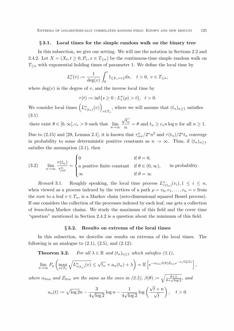
In this subsection, we give our setting. We will use the notation in Sections 2.2 and2.4.2. Let X=(X_{t}, t\geq 0, P_{x}, x\in T_{\leq n}) be the continuous‐time simple random walk on
T_{\leq n} with exponential holding times of parameter 1. We define the local time by
L_{t}^{n}(v) := \frac{1}{\deg(v)} 0^{t_{1_{\{X_{s}=v\}}ds}} ’ t>0, v\in T_{\leq n},
where \deg(v) is the degree of v , and the inverse local time by
\tau(t) :=\inf\{s\geq 0 : L_{s}^{n}(\rho) >t\}, t>0.
We consider local times (L_{\tau(t_{n})}^{n}(v))_{v\in T_{n}} , where we will assume that (t_{n})_{n\geq 1} satisfies
(3.1)
there exist \theta\in [0, \infty], c_{*} >0 such that \lim_{n} \frac{t_{n}}{n} =\theta and t_{n} \geq c_{*}n\log n for all n\geq 1.
Due to (2.15) and [29, Lemma 2.1], it is known that \tau_{cov}^{n}/2^{n}n^{2} and \tau(t_{n})/2^{n}t_{n} convergein probability to some deterministic positive constants as n arrow 1 . Thus, if (t_{n})_{n\geq 1}satisfies the assumptio > (3.1) , then
(3.2) \lim_{n} \frac{\tau(t_{n})}{\tau_{cov}^{n}}= \{\begin{array}{ll}0 if \theta=0,a positive finite constant if \theta\in (0, \infty) ,\infty \end{array}if \theta=\infty
in probability:
Remark 3.1. Roughly speaking, the local time process L_{\tau(t_{n})}^{n} (vi), 1 \leq i \leq n,
when viewed as a process indexed by the vertices of a path \rho=v_{0}, v_{1} , :::, v_{n}=v from
the root to a leaf v\in T_{n} , is a Markov chain (zero‐dimensional squared Bessel process).If one considers the collection of the processes indexed by each leaf, one gets a collection
of branching Markov chains. We study the maximum of this field and the cover time“question” mentioned in Section 2.4.2 is a question about the minimum of this field.
§3.2. Results on extrema of the local times
In this subsection, we describe our results on extrema of the local times. The
following is an analogue to (2.1), (2.5), and (2.12):
Theorem 3.2. For all \lambda\in \mathbb{R} and (t_{n})_{n\geq 1} which satisfies (3.1),
\lim_{narrow\infty}P_{\rho} ( \max_{v\in T_{n}}\sqrt{L_{\tau(t_{n})}^{n}(v)}\leq t_{n}+a_{n}(t_{n})+\lambda) =E[e^{-\alpha_{brw}\beta(\theta)Z_{brw}e^{-2\sqrt{\log 2}\lambda}}] ,
where \alpha_{brw} and Z_{brw} are the same as the ones in (2.5), \beta(\theta) := \sqrt{\frac{\theta+l}{\theta+\sqrt{\log 2}}} , and
a_{n}(t) := \log 2n-\frac{3}{4\log 2}\log n-\frac{l}{4\log 2}\log(\frac{t+n}{t}) , t>0.

126 Yoshihiro Abe
Comparing Theorem 3.2 with (2.5), when \theta=1 (that is, when \tau(t_{n}) is much largerthan the cover time due to (3.2)), one can see that the limiting law of the maximumof local times are the same as that of the BRW on T and that a_{n}(t_{n}) =m_{n}^{brw} , where
m_{n}^{brw} is the one in (2.6). This similarity is plausible in view of the Dynkin isomorphism[34, 35] which relates local times with the BRW. However, when \theta is finite, we have adifference from the BRW since \beta(\theta) \neq 1, a_{n}(t_{n}) \neq m_{n}^{brw} . The term \beta(\theta) comes from
the Radon‐Nikodym derivative of the law of a zero‐dimensional squared Bessel process
with respect to that of a one‐dimensional squared Bessel process (recall Remark 3.1).Let \omega_{1oc}(\lambda) be the limiting law in Theorem 3.2. We further show that
1 — \omega_{1oc}(\lambda)\sim\alpha_{brw}\beta(\theta)\lambda e^{-2\sqrt{\log 2}\lambda} as \lambdaarrow 1.
Thus, the tail of the limiting law \omega_{1oc} has an asymptotic behavior similar to those 0
the BBM, the BRW, and the two‐dimensional DGFF, cf. (2.3), (2.8), (2.13).We have a stronger result on extrema of the local times. Recall (2.9). We consider
the point process on [0 , 1 ] \cross \mathbb{R}
--n,t-(m) := \sum_{u\in T_{n-m}}\delta(\sigma(\arg\max_{u}L_{\tau t}^{n}), \max_{v\in\tau_{7m}^{u}\sqrt{L_{\tau t}^{n}(v)}-} t-a_{n}(t)) ’ t>0, 0\leq m\leq n,
where for each u \in T_{n-m} , we set T_{m}^{u} := \{uw : w \in T_{m}\} , and \arg\max_{u}L_{\tau(t)}^{n} is the
maximizer on T_{m}^{u} , that is, the vertex v_{*} \in T_{m}^{u} such that L_{\tau(t)}^{n}(v_{*}) = \max_{v\in T_{m}^{u}}L_{\tau(t)}^{n}(v) .
We now state the main result of [1]:
Theorem 3.3. For all (r_{n})_{n\geq 1} with \lim_{narrow\infty}r_{n}=1 and \lim_{narrow\infty}r_{n}/n=0 and
(t_{n})_{n\geq 1} which satis(es (3.1), as narrow 1,
--n,t_{n}-(r_{n}) law PPP (\alpha_{brw}\beta(\theta)Z_{\infty,1}(dx)\otimes 2 \log 2e^{-2\sqrt{\log 2}h}dh) in M_{+}([0,1] \cross \mathbb{R}) ,
where \alpha_{brw} and \beta(\theta) are the same as the ones in Theorem 3.2, and Z_{\infty,1} is the critica
random multiplicative cascade measure in (2.10).
Theorem 3.3 is an analogue of (2.14) for the two‐dimensional DGFF and [5, Theo‐rem 2] for the BBM. Our results are inspired by [18].
Acknowledgment. The author would like to thank the referee for valuable comments.
References
[1] Y. Abe. Extremes of local times for simple random walks on symmetric trees. Preprint.[2] E. Aidékon. Convergence in law of the minimum of a branching random walk. Ann. Probab.
41 (2013), 1362‐1426.

Extrema of logarithmically correlated random FiELD: Known and new results 127
[3] E. Aidékon, J. Berestycki, É. Brunet and Z. Shi. Branching Brownian motion seen fromits tip. Probab. Theory Relat. Fields. 157 (2013), 405‐451.
[4] L.‐P. Arguin, A. Bovier, and N. Kistler. Genealogy of extremal particles of branchingBrownian motion. Commun. Pure Appl. Math. 64 (2011), 1647‐1676.
[5] L.‐P. Arguin, A. Bovier, and N. Kistler. Poissonian statistics in the extremal process ofbranching Brownian motion. Ann. Appl. Probab. 22 (2012), 1693‐1711.
[6] L.‐P. Arguin, A. Bovier, and N. Kistler. The extremal process of branching Brownianmotion. Probab. Theory Relat. Fields. 157 (2013), 535‐574.
[7] M. Bachmann. Limit theorems for the minimal position in a branching random walk withindependent logconcave displacements. Adv. in Appl. Probab. 32 (2000), 159‐176.
[8] J. Barral, R. Rhodes, and V. Vargas. Limiting laws of supercritical branching randomwalks. C. R. Acad. Sci. Paris, Ser. I. 350 (2012), 535‐538.
[9] J. Barral, A. Kupiainen, M. Nikula, E. Saksman, and C. Webb. Critical Mandelbrotcascades. Commun. Math. Phys. 325 (2014), 685‐711.
[10] I. Benjamini and O. Schramm. KPZ in one dimensional random eometry of multiplicativecascades. Commun. Math. Phys. 289 (2009), 653‐662.
[11] D. Belius and N. Kistler. The subleadin order of two dimensional cover times.arXiv: 1405. 0888vl.
[12] J. D. Biggins and A. E. Kyprianou. Fixed points of the smoothin transform: the boundarycase. Electron. J. Probab. 10 (2005), 609‐631.
[13] M. Biskup and O. Louidor. Extreme local extrema of two‐dimensional discrete Gaussianfree field. Commun. Math. Phys. (to appear)
[14] M. Biskup and O. Louidor. Conformal symmetries in the extremal process of two‐dimensional discrete Gaussian free field. arXiv:1410.4676
[15] E. Bolthausen, J.‐D. Deuschel, and G. Giacomin. Entropic repulsion and the maximumof the two‐dimensional harmonic crystal. Ann. Probab. 29 (2001), 1670‐1692.
[16] E. Bolthausen, J.‐D. Deuschel, and O. Zeitouni. Recursions and tightness for the maximumof the discrete, two dimensional Gaussian free field. Electron. Commun. Probab. 16 (2011),114‐119.
[17] A. Bovier. From spin glasses to branching Brownian motion — and back/p In: RandoWalks, Random Fields, and Disordered Systems, M. Biskup, J. Černy, R. Kotecky, Eds.,Lecture Notes in Mathematics 2144, Springer, 2015.
[18] A. Bovier and L. Hartung. Extended convergence of the extremal process of branchingBrownian motion. arXiv: 1412.5975
[19] A. Bovier and I. Kurkova. Derrida’s generalized random energy models. 1. Models withfinitely many hierarchies. Ann. Inst. H. Poincaré Probab. Statist. 40 (2004), 439‐480.
[20] A. Bovier and I. Kurkova. Derrida’s generalized random energy models. 2. Models withcontinuous hierarchies. Ann. Inst. H. Poincaré Probab. Statist. 40 (2004), 481‐495.
[21] M. Bramson. Convergence of solutions of the Kolmogorov equation to traveling waves.Mem. Amer. Math. Soc. 44 (1983)
[22] M. Bramson and O. Zeitouni. Tightness for a family of recursion equations. Ann. Probab.37 (2009), 615‐653.
[23] M. Bramson and O. Zeitouni. Tightness of the recentered maximum of the two‐dimensionaldiscrete Gaussian free field. Commun. Pure Appl. Math. 65 (2012), 1‐20.
[24] M. Bramson, J. Ding, and O. Zeitouni. Convergence in law of the maximum of the two‐dimensional discrete Gaussian free field. Commun. Pure Appl. Math. 69 (2016), 62‐123.
[25] M. Bramson, J. Ding, and O. Zeitouni. Convergence in law of the maximum of nonlattice

128 Yoshihiro Abe
branching random walk. Ann. Inst. H. Poincaré Probab. Statist. (to appear)[26] D. Buraczewski. On tails of fixed points of the smoothing transform in the boundary case.
Stochastic Process. Appl. 119 (2009), 3955‐3961.[27] A. Dembo, Y. Peres, J. Rosen, and O. Zeitouni. Thick points for planar Brownian motion
and the Erós‐Taylor conjecture on random walk. Acta Math., 186 (2001), 239‐270.[28] A. Dembo, Y. Peres, J. Rosen, and O. Zeitouni. Cover times for Brownian motion and
random walks in two dimensions. Ann. Math. 160 (2004), 433‐464.[29] J. Ding. Asymptotics of cover times via Gaussian free fields: Bounded‐degree graphs and
general trees. Ann. Probab. 42 (2014), 464‐496.[30] J. Ding and O. Zeitouni. A sharp estimate for cover times on binary trees. Stochastic
Processes and their Applications. 122 (2012), 2117‐2133.[31] J. Ding and O. Zeitouni. Extreme values for two‐dimensional discrete Gaussian free field.
Ann. Probab. 42 (2014), 1480‐1515.[32] B. Duplantier and S. Sheffield. Liouville quantum ravity and KPZ. Invent. Math. 185
(2011), 333‐393.[33] R. Durrett and T. M. Liggett. Fixed points of the smoothin transformation. Z.
Wahrscheinlichkeitstheor. Verw. Geb. 64 (1983), 275‐301.[34] E. B. Dynkin. Markov processes as a tool in field theory. J. Funct. Anal. 50 (1983),
167‐187.
[35] N. Eisenbaum, H. Kaspi, M. B. Marcus, J. Rosen, and Z. Shi. A Ray‐Knight theorem forsymmetric Markov processes. Ann. Probab. 28 (2000), 1781‐1796.
[36] J.‐P. Kahane and J. Peyrière. Sur certaines martingales de Benoit Mandelbrot. Adv. Math.22 (1976), 131‐145.
[37] N. Kistler. Derrida’s random energy models from spin lasses to the extremes of correlatedrandom fields, in Correlated Random Systems: Five Different Methods, V. Gayrard, N.Kistler, editors. Lecture Notes in Mathematics, vol. 2143 (Springer, Berlin, 2015), pp.71‐120.
[38] S.P. Lalley and T. Sellke. A conditional limit theorem for the frontier of a branchingBrownian motion. Ann. Probab. 15 (1987), 1052‐1061.
[39] Q. Liu. On generalized multiplicative cascades. Stochastic Process. Appl. 86 (2000), 263‐286.
[40] T. Madaule. Convergence in law for the branching random walk seen from its tip. J. Theor.Probab. (to appear)
[41] H. P. McKean. Application of Brownian motion to the equation of Kolmogorov‐Petrovskii‐Piskunov. Comm. Pure Appl. Math. 28 (1976), 323‐331.
[42] O. Zeitouni. Branching random walks and Gaussian free fields. Available at http: //www.
wisdom. weizmann. ac. il/\sim zeitouni/pdf/notesBRW. pdf


![Xvii samet dr. yoshihiro yamazake [mini-curso 6ª -feira] 2wps ufpel-2010_apres2](https://static.cupdf.com/doc/110x72/54963b1fb47959962d8b5d9c/xvii-samet-dr-yoshihiro-yamazake-mini-curso-6a-feira-2wps-ufpel-2010apres2.jpg)