arX
iv:1
604.
0056
3v1
[ast
ro-p
h.S
R]
2 A
pr 2
016
EXPLORING THE ORIGIN ANDDYNAMICS OF SOLAR MAGNETIC
FIELDS
Soumitra Hazra
Department of Physical Sciencesand
Centre of Excellence in Space Sciences India
Indian Institute of Science Education and Research Kolkata
This dissertation is submitted for the degree of
Doctor of Philosophy in Science
2015


Dedicated to My Parents...


Declaration
This thesis is a presentation of my original research work. Wherever contributions of others
are involved, every effort is made to indicate this clearly,with due reference to the literature
and acknowledgments of collaborative research and discussions. The work has not been
submitted earlier either in entirety or in parts for a degreeor diploma at this or any other
Institution or University. Some chapters of this thesis have either been published or are in
the process of being published. This work was done under the guidance of Dr. Dibyendu
Nandi, at the Indian Institute of Science Education and Research Kolkata (IISER Kolkata).
Soumitra Hazra
2015

CERTIFICATE FROM THE SUPERVISOR
This is to certify that this thesis entitled"Exploring the Origin and Dynamics of Solar
Magnetic Fields" – which is being submitted by Soumitra Hazra (who registeredon 11th
August, 2009 for a PhD Degree with registration number09RS028at the Indian Institute of
Science Education and Research Kolkata) – is based upon his own research work under my
supervision and that neither this thesis nor any part of it has been submitted for any degree
or any other academic award anywhere else.
Dr. Dibyendu Nandi
Associate Professor
Department of Physical Sciences and Center of Excellence inSpace Sciences India
Indian Institute of Science Education and Research Kolkata
West Bengal 741246
India


Acknowledgements
This is a special moment for me and I wish to express my sinceregratitude to my thesis
supervisor Dibyendu Nandi, who introduced me to the exciting world of research in Astro-
physics. This thesis work would never have been possible without his help and constant
support during this period. He also taught me that one of the major components of scientific
research is to be able to communicate your scientific ideas with others. I have learnt a lot of
science as well as the methodolgy of tackling a difficult problem through discussions with
him. I also thank him for his support and encouragement to attend different conferences
which enabled me to interact with other scientists.
I would like to thank B Ravindra for giving me the opportunityto visit his institute and
work with him. His constant help, encouragement and discussion helped me grasp the skills
of satelite data anyalisis quickly. I have completed an important project with him "The Re-
lationship between Solar Coronal X-Ray Brightness and Active Region Magnetic Fields: A
Study with High Resolution Hinode Observations". I am also extremly thankful to Aveek
da, Andres, Piet, Dario, Bidya da, Dipankar da, Shravan Hanasoge, Paul Rajaguru, Durgesh
Tripathi, Nandita Srivastava, Dhrubaditya Mitra and Prasad Subramanian for their helpful
discussions and readiness to answer my numerious queries. Ialso want to thank Arnab Rai
Choudhuri for his two books "Physics of Fluids and Plasma’ and "Astrophysics for Physi-
cist" which I used as a text book during my Ph.D period.
I am also greatful to all the faculty members and colleagues of the Department of Physi-
cal Sciences, IISER Kolkata for their help and support. I want to thank Barun (nada), Dyuti,
choto and baro Nandan (Das & Roy), Abhinav, Subhrajit (kaka), Gopal, Tanmoy, Sudipta,
Rupak, Richarj, Sumi, Harkirat, Sanhita, Anirudha, Abhishek, Arghya da (mama), Basu
da, Chandan da, Rabi da, Vivek da, Priyam da for making my initial life at IISER Kolkata
fun and enjoyable. It gives me pleasure to thank my CESSI lab mates Mayukh, Prantika,
Avyarthana, Rakesh, Sushant, Tamoghna, Athira, Sanchita,Prasenjit, Abhinna, Chandu da
for their support. A special word of thanks to Mayukh and Prantika for their readiness to
help me with MATLAB related issues. Mayukh has also collaborated with me in a paper. I

x
want to thank Sanjib Ghosh for his initial help in my first work. I also thank Madhusudan,
Arun Babu, Wageesh, Sushant Bishoi, Grijesh Gupta, Krishnada, Vemareddy for discussion
and help. It is also my pleasure to thank Ankan, Debmalya (motu), Chiranjeeb, Soumya
(gambat), Diptesh, Deepak, Radhe, Soumen, Rafikul and all those who made my life mem-
orable and enjoyable at IISER Kolkata. I also want to thank Prasanta da and Soma di for
their help and support during my stay at Montana.
It is also my pleasure to thank my masters and bachelors degree friends Monalisa,
Arup, Amit, Amaresh, Arnab, Nikhil, Sarengi, Suman, Prithwish da, Asim da, Samaresh
da and my childhood friends Palash, Dilip, Jagneswar, Gopi,Bubun, Bulbul da, Bappaditya,
Sushanta, Arup Samanta, Dipak da, Abhi, Piu for their help and support. I also want to
thank my maternal uncles and aunts (mama and mamima), paternal uncles and aunts for
their encouragement and support.
Finally, I would like to thank my parents and sister for theirconstant patience and sup-
port. They have always shared my joys and sorrows and have given their unconditional love.
Thanks to all of my family members and friends for their understanding and supporting me.
Abstract
The Sun is a magnetically active star and is the source of the solar wind, electromagnetic ra-
diation and energetic particles which affect the heliosphere and the Earth’s atmosphere. The
magnetic field of the Sun is responsible for most of the dynamic activity of the Sun. This
thesis research seeks to understand solar magnetic field generation and the role that mag-
netic fields play in the dynamics of the solar atmosphere. Specifically, this thesis focuses on
two themes: in the first part, we study the origin and behaviour of solar magnetic fields us-
ing magnetohydrodynamic dynamo theory and modelling, and in the second part, utilizing
observations and data analysis we study two major problems in solar physics, namely, the
coronal heating problem and initiation mechanisms of solarflares.
The magnetic field of the Sun, whose evolution is evident in the 11 year cycle of
sunspots, is created within the Sun through complex interactions between internal plasma
flows and fields. It is widely believed that magnetic fields of not just the Sun, but all as-
tronomical bodies are produced by this hydromagnetic dynamo process. To explain the
origin of the solar cycle, Eugene Parker first proposed the idea of flux recycling between
the toroidal (which is in the azimuthal i.e.,φ -direction) and poloidal (which is in r-θ plane)
field components . Currently, flux transport dynamo models based on the Babcock-Leighton
mechanism for poloidal field generation appears as a promising candidate for explaining dif-
ferent aspects of the solar cycle. In this scenario, the toroidal field is produced within the
convection zone due to stretching of the poloidal componentby strong differential rotation
while the poloidal field is produced at the solar surface due to decay and dispersal of tilted
bipolar sunspot pairs. Flux transport mechanisms such as diffusion, meridional flow and tur-
bulent pumping shares the role of communicator between these two largely separated source
layers. In chapter 1, we describe observations of solar magnetic fields and development of
solar dynamo theory to motivate our work.
An outstanding issue related to the solar cycle is extreme fluctuations, specifically the
occurrence of extended periods of reduced or no activity, known as grand minima episodes.
The origin of such episodes have eluded a consistent theory.The Maunder minima was
xii
such an episode during 1645-1715 AD when there was almost no sunspots observed on the
Sun. There is also observational evidence of many such episodes in the past. The crucial
fact is that the solar cycle has recovered from these episodes every time and regained nor-
mal activity levels. It is expected that during grand minimaphases, the Babcock-Leighton
mechanism would not be able to produce poloidal field as this mechanism relies on the
presence of sunspots on the solar surface. This leads to the following fundamental ques-
tion: How does the solar cycle recover every time from these episodes? We address this
question through diverse means. In chapter 2 of this thesis,we develop a mathematical,
low order time delay dynamo model (based on delay differential equations) removing all
spatial dependence terms from the magnetic induction equation and mimic flux transport
through the introduction of finite time delays in the system.By introducing fluctuations in
the Babcock-Leighton source term of this low order dynamo model, we, for the first time
explicitly demonstrate that a solar cycle model based on theBabcock-Leighton mechanism
alone can not recover from a grand minima. We find that an additional poloidal field gener-
ation mechanism effective on weak magnetic field is necessary for recovery of the sunspot
cycle from grand minima like episodes.
Modeling the Babcock-Leighton mechanism in a correct way tocapture the observed
surface dynamics is a challenging task. Two different approaches, mainly near-surface
alpha-coefficient formulation and the double ring formalism has been followed to model
the Babcock-Leighton mechanism for poloidal field generation. Earlier it has been shown
that the second approach, i.e., the double ring formalism ismore successful in explaining
observational results compared to the near-surface alpha-coefficient formulation. Inspired
by this, we develop a 2.5D kinematic solar dynamo model wherewe simulate the Babcock-
Leighton mechanism via the double ring algorithm. In chapter 3 of this thesis, we utilize
this state-of-the spatially extended model in a solar like geometry to validate our findings
on entry and exit from Maunder minima like episodes. We find that stochastic fluctuations
in the Babcock-Leighton mechanism is a possible candidate for triggering entry into grand
minima phases. However, the Babcock-Leighton mechanism alone is not able to recover
the solar cycle from a grand minimum. An additional mean fieldα-effect effective on week
magnetic field is necessary for self-consistent recovery. Thus, this result puts the earlier
findings based on a low order time delay model on firmed grounds. This spatially extended
model also allows one to explore latitudinal asymmetry and hemispheric coupling of the
sunspot cycle. Based on simulations with this model, we find that stochastic fluctuation in
both poloidal field sources makes hemispheric coupling weak, thus introducing asymmetry
in sunspot eruptions in the Northern and Southern hemispheres. The phase locking between
xiii
the two hemispheres is thus impacted resulting in a switching of the parity of the solutions.
Particularly we find that parity shifts in the sunspot cycle is more likely to occur when solar
activity in one hemisphere strongly dominates over the other hemisphere for a period of
time significantly longer than the sunspot cycle timescale.While direct observations over
the last fifty years have shown that the solar magnetic cycle exhibits dipolar (odd) parity, our
results suggest that the solar cycle has a significant probability to reside in the quadrapolar
(even) parity state. Our findings may open the pathway for predicting parity flip in the Sun.
Meridional circulation is an essential ingredient in present day kinematic solar dynamo
models. Earlier studies based on theoretical considerations and numerical simulations have
suggested that a deep equatorward meridional flow near the base of the solar convection
zone is plausibly essential in explaining the observed equatorward migration of the sunspot
belt. However there is no observational evidence of such a deep meridional flow as it is
difficult to probe such deep layers. Some recent observational studies, on the other hand, in-
dicate that the meridional flow could be shallow or more complex than previously assumed.
In chapter 4 of this thesis, we explore whether flux transportdynamos could function with
such a shallow meridional flow and discuss the consequences that this scenario would have
on our traditional understanding of magnetic field dynamicsin the solar interior. We demon-
strate that dynamo models of the solar cycle can produce solar-like solutions with a shallow
meridional flow if the effects of turbulent pumping of magnetic flux is taken into account.
In the second part of this thesis, we utilize satellite observations to explore the dynamics
of magnetic fields in the solar atmosphere. The solar corona,the outer atmosphere of the
Sun is very hot compared to the solar surface and can reach millions of degrees. There is
controversy regarding the physical processes that heat thesolar outer atmosphere to such
high temperatures. Such high temperatures result in X-ray emission from the solar corona.
In chapter 5, we discuss the observational techniques and the current theoretical understand-
ing developed over time, necessary to explain coronal dynamics. In chapter 6 of this thesis,
we explore the relationship between coronal X-ray brightness and sunspot magnetic fields
using high resolution observations from the Solar Optical Telescope and X-Ray Telescope
onboard the Hinode satellite (a joint JAXA-NASA space mission). We find that the total
magnetic flux within active regions sunspot structures is the primary determinant of solar
coronal X-ray luminosity suggesting that magnetic flux is the fundamental quantity that
determines coronal heating. This result sets important constraints on theories of solar and
stellar coronal heating.
xiv
Solar flares are highly energetic eruptions from the Sun thathurl out magnetize plasma
and emit high energy radiation thereby impacting space weather and space- and some
ground-based technologies. Thus predictions of solar flareis necessary for developing ad-
vance warning systems. Previous studies indicate that the non-potentiality of the magnetic
field is closely related with solar flare productivity. However traditional measures of mag-
netic field non-potentiality based on the force-free parameter have been questioned and stud-
ies based on the force-free parameter have given diverging results. In chapter 7 of this thesis,
a recently developed, flux-tube fitting technique is utilized to measure the non-potentiality
(twist) of solar magnetic fields and test whether the kink-instability mechanism (follow-
ing magnetic helicity conservation) can be a plausible initiation mechanism for solar flares.
We demonstrate that those sunspot magnetic field structuresin which the twist exceeds the
threshold for kink instability are more prone to generate solar flares. This finding may lead
to more accurate solar flare prediction schemes based on the kink instability mechanism.
The chapters that follow, outline the outcome of this thesisresearch, are written in the
form of research publications; as such they are self-contained with independent introduc-
tions and conclusions.
Research publications emnating out of this thesis work:
• A stochastically forced time delay solar dynamo model: self-consistent recovery from
a Maunder-like grand minimum necessitates a mean-field alpha effect. Hazra, S.,
Passos, D. & Nandy, D.ApJ, 789, 5 (2014)
(Dario Passos was a collaborator in exploring this idea using a different, spatially
extended dynamo model the results of which are published in Passos, D, Nandy, D,
Hazra, S & Lopes, I. 2014, A&A, 563, A18.)
• Double ring algorithm of solar active region eruptions within the framework of kine-
matic dynamo model. Hazra, S. & Nandy, D.,Bulletin of Astronomical Society of
India, ASI conference series, vol 10, p 117-121 (2013)
• The Relationship between Solar Coronal X-Ray Brightness and Active Region Mag-
netic Fields: A Study Using High Resolution Hinode Observations. Hazra, S., Nandy,
D. & Ravindra, B.Solar Physics, 290, 771 (2015)
(Ravindra Belur was a collaborator in this work in which he provided the knowhow
on the software tools necessary to reduce the observationaldata.)
• A New Paradigm of Magnetic Field Dynamics at the Basis of theSunspot Cycle.
Hazra, S. & Nandy, D. in preparation

xv
• Strong Hemispheric Asymmetry can Trigger Parity Changes in the Sunspot Cycle.
Hazra, S. & Nandy, D. in preparation
• Exploring the Relationship between Kink Instability and Solar Flare: A Study Using
High Resolution Hinode Observations. Panja, M., Hazra, S. &Nandy, D. in prepara-
tion
(Mayukh Panja was an undergraduate summer student who contributed to the obser-
vational analysis under the supervision of Soumitra Hazra and Dibyendu Nandy.)

Table of contents
List of figures xxi
List of tables xxix
Nomenclature xxix
1 Introduction to the Solar Magnetic Cycle 1
1.1 The Sun: Interior and Atmosphere . . . . . . . . . . . . . . . . . . . .. . 1
1.1.1 Solar Interior . . . . . . . . . . . . . . . . . . . . . . . . . . . . . 1
1.1.2 Solar Atmosphere . . . . . . . . . . . . . . . . . . . . . . . . . . .1
1.2 Discovery of the Solar Magnetic Cycle . . . . . . . . . . . . . . . .. . . . 2
1.3 Generation of the Large Scale Solar Magnetic Field . . . . .. . . . . . . . 5
1.3.1 Magnetohydrodynamics . . . . . . . . . . . . . . . . . . . . . . .5
1.3.2 Parker’s Mean-Field Dynamo . . . . . . . . . . . . . . . . . . . .7
1.3.3 Mean Field Electrodynamics . . . . . . . . . . . . . . . . . . . . .9
1.3.4 Flux Tube Dynamics and the Babcock-Leighton Mechanism for Poloidal
Field Generation . . . . . . . . . . . . . . . . . . . . . . . . . . .11
1.3.5 Differential Rotation and Meridional Circulation: Essential Ingredi-
ents of Solar Dynamo Modelling . . . . . . . . . . . . . . . . . . .13
1.3.6 Kinematic Babcock-Leighton Dynamo Models . . . . . . . . .. . 14
2 Exploring Grand Minima Phases with a Low Order, Time Delay Dynamo Model 21
2.1 Introduction . . . . . . . . . . . . . . . . . . . . . . . . . . . . . . . . . .21
2.2 Stochastically Forced, Non-Linear, Time Delay Solar Dynamo Model . . . 24
2.3 Results and Discussions . . . . . . . . . . . . . . . . . . . . . . . . . . .. 28
2.4 Conclusions . . . . . . . . . . . . . . . . . . . . . . . . . . . . . . . . . .32
3 Strong Hemispheric Asymmetry can Trigger Parity Changes in the Sunspot
Cycle 35
xviii Table of contents
3.1 Introduction . . . . . . . . . . . . . . . . . . . . . . . . . . . . . . . . . .36
3.2 Model . . . . . . . . . . . . . . . . . . . . . . . . . . . . . . . . . . . . .38
3.2.1 Modelling Active Regions as Double Rings and Recreating the poloidal
field . . . . . . . . . . . . . . . . . . . . . . . . . . . . . . . . . . 39
3.3 Results and Discussion . . . . . . . . . . . . . . . . . . . . . . . . . . . .41
3.4 Conclusions . . . . . . . . . . . . . . . . . . . . . . . . . . . . . . . . . .49
4 A New Paradigm of Magnetic Field Dynamics at the Basis of theSunspot Cycle
Based on Turbulent Pumping 51
4.1 Introduction . . . . . . . . . . . . . . . . . . . . . . . . . . . . . . . . . .52
4.2 Results . . . . . . . . . . . . . . . . . . . . . . . . . . . . . . . . . . . . .53
4.3 Discussions . . . . . . . . . . . . . . . . . . . . . . . . . . . . . . . . . .60
5 Observational Studies of Magnetic Field Dynamics in the Solar Atmosphere 63
5.1 Measuring large scale solar magnetic field . . . . . . . . . . . .. . . . . . 63
5.2 Effects of large scale solar magnetic field . . . . . . . . . . . .. . . . . . 64
5.2.1 Null Points and Current Sheet . . . . . . . . . . . . . . . . . . . .64
5.2.2 Magnetic Reconnection . . . . . . . . . . . . . . . . . . . . . . .65
5.2.3 Magnetic Nonpotentiality . . . . . . . . . . . . . . . . . . . . . .67
5.2.4 Magnetic Helicity . . . . . . . . . . . . . . . . . . . . . . . . . . .69
5.2.5 The Coronal Heating Problem . . . . . . . . . . . . . . . . . . . .70
5.2.6 Solar Flares . . . . . . . . . . . . . . . . . . . . . . . . . . . . . .72
6 The Relationship between Solar Coronal X-Ray Brightness and Active Region
Magnetic Fields 73
6.1 Introduction . . . . . . . . . . . . . . . . . . . . . . . . . . . . . . . . . .74
6.2 Data Analysis . . . . . . . . . . . . . . . . . . . . . . . . . . . . . . . . .76
6.2.1 Data Selection . . . . . . . . . . . . . . . . . . . . . . . . . . . .76
6.2.2 Data Coalignment . . . . . . . . . . . . . . . . . . . . . . . . . .77
6.3 Integrated Quantities . . . . . . . . . . . . . . . . . . . . . . . . . . . .. 80
6.3.1 Active-Region Coronal X-Ray Brightness . . . . . . . . . . .. . . 80
6.3.2 Global Magnetic-Field Quantities . . . . . . . . . . . . . . . .. . 80
6.4 Results . . . . . . . . . . . . . . . . . . . . . . . . . . . . . . . . . . . . .82
6.4.1 Correlation Between Global Magnetic Field Quantities and X-ray
Brightness . . . . . . . . . . . . . . . . . . . . . . . . . . . . . .83
6.4.2 Correlations Among Global Magnetic-Field Quantities and Partial
Correlation Analysis . . . . . . . . . . . . . . . . . . . . . . . . .86
Table of contents xix
6.4.3 Filter Issues in the X-ray Data . . . . . . . . . . . . . . . . . . . .88
6.5 Summary and Discussion . . . . . . . . . . . . . . . . . . . . . . . . . . .89
7 Kink Instability, Coronal Sigmoids and Solar Eruptive Events 91
7.1 Introduction . . . . . . . . . . . . . . . . . . . . . . . . . . . . . . . . . .91
7.2 Data Selection and Analysis . . . . . . . . . . . . . . . . . . . . . . . .. 93
7.3 Methods . . . . . . . . . . . . . . . . . . . . . . . . . . . . . . . . . . . .94
7.3.1 Measuring Twist by Cylindrical-Flux-Tube-Fitting Technique . . . 94
7.3.2 Establishing the Kink Instability Criterion . . . . . . .. . . . . . . 95
7.4 Results . . . . . . . . . . . . . . . . . . . . . . . . . . . . . . . . . . . . .97
7.5 Summary and Discussions . . . . . . . . . . . . . . . . . . . . . . . . . .99
Appendix A Numerical Methods 103
References 109


List of figures
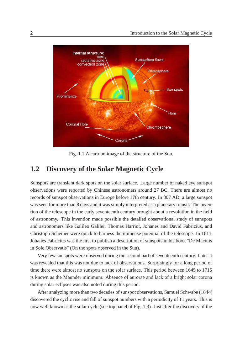
1.1 A cartoon image of the structure of the Sun. . . . . . . . . . . . .. . . . . 2
1.2 SDO-HMI magnetogram image recorded on May 11, 2015 showing bipolar
sunspot pairs within active region structures. In the image, white signifies
positive polarity while black signifies negative polarity sunspots. . . . . . . 3
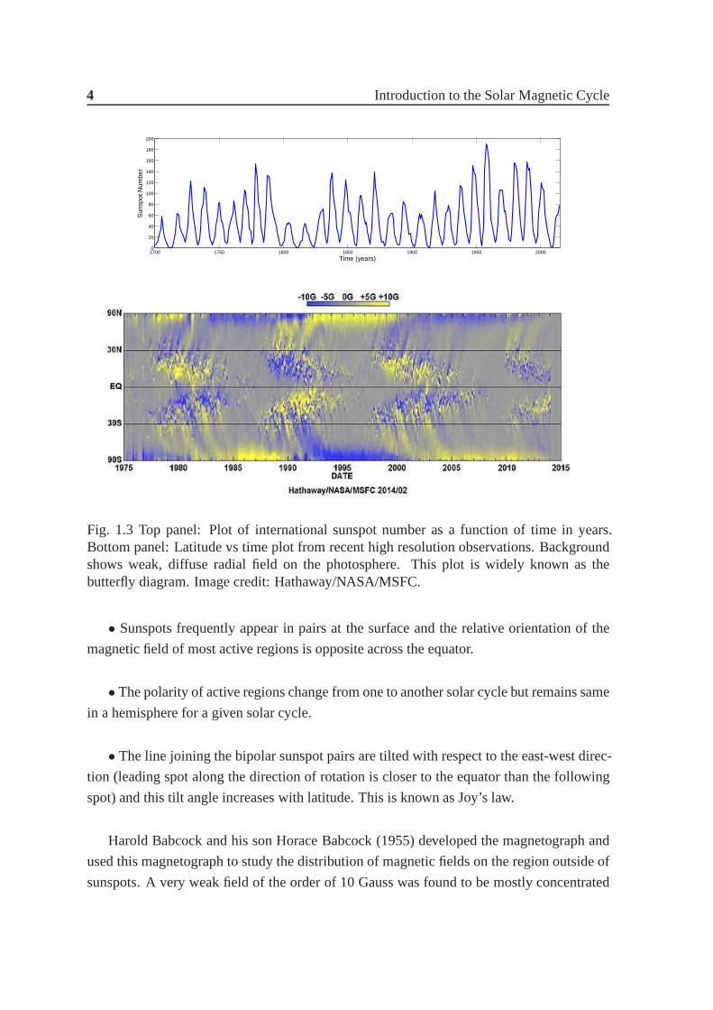
1.3 Top panel: Plot of international sunspot number as a function of time in
years. Bottom panel: Latitude vs time plot from recent high resolution ob-
servations. Background shows weak, diffuse radial field on the photosphere.
This plot is widely known as the butterfly diagram. Image credit: Hath-
away/NASA/MSFC. . . . . . . . . . . . . . . . . . . . . . . . . . . . . . 4
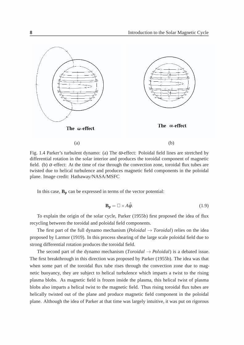
1.4 Parker’s turbulent dynamo: (a) Theω-effect: Poloidal field lines are stretched
by differential rotation in the solar interior and producesthe toroidal com-
ponent of magnetic field. (b)α-effect: At the time of rise through the con-
vection zone, toroidal flux tubes are twisted due to helical turbulence and
produces magnetic field components in the poloidal plane. Image credit:
Hathaway/NASA/MSFC . . . . . . . . . . . . . . . . . . . . . . . . . . . 8
1.5 A cartoon image of the Babcock-Leighton mechanism: (a) Newly emerged
bipolar magnetic regions with opposite leading/ followingpolarity patterns
obeying Hale’s polarity law. (b) Decaying bipolar magneticregions, Trail-
ing polarity goes to higher latitude while leading components reconnect
across the equator. Image credit: Paul Charbonneau . . . . . . .. . . . . . 12
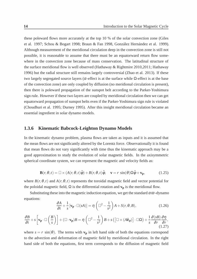
1.6 (a) Variation of turbulent magnetic diffusivity diffusivity with radius. (b)
Analytical differential rotation profile (in nHz) used in dynamo model. Re-
gion between two dashed circular arcs indicates the tachocline. . . . . . . . 15
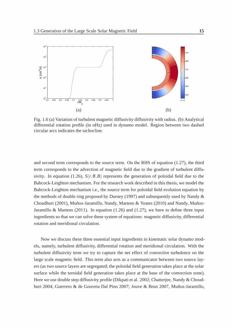
1.7 (a) Meridional circulation streamlines used in our model. Region between
two dashed circular arcs indicates the tachocline. (b) Plotof latitudinal ve-
locity (vθ in m/s) as a function ofr/R0 at 450 latitude. . . . . . . . . . . . . 17
xxii List of figures
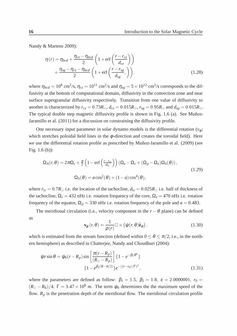
1.8 Plot of latitudinal velocity (vθ in m/s) as a function of latitude (θ ) at the
solar surface. . . . . . . . . . . . . . . . . . . . . . . . . . . . . . . . . .17
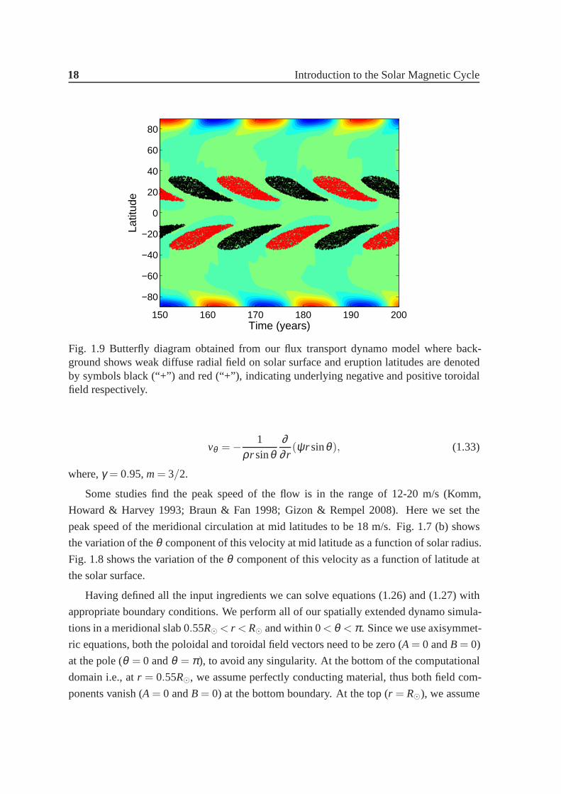
1.9 Butterfly diagram obtained from our flux transport dynamomodel where
background shows weak diffuse radial field on solar surface and eruption
latitudes are denoted by symbols black (“+”) and red (“+”), indicating un-
derlying negative and positive toroidal field respectively. . . . . . . . . . . 18
1.10 Butterfly diagram obtained from our flux transport dynamo model where
background shows weak diffuse radial field on solar surface and eruption
latitudes are denoted by symbols black (“+”) and red (“+”), indicating under-
lying negative and positive toroidal field respectively. This plot is obtained
using the meridional flow profile suggested by Muñoz-Jaramillo et al. (2009).19
2.1 Profile of the quenching functionf1 for the Babcock-Leightonα and f2 for
the weak, mean fieldα-effect (described later in the text). The plot off1corresponds to parametersBmin = 1 andBmax= 7 and f2 corresponds to
Beq= 1 (all in arbitrary code units). . . . . . . . . . . . . . . . . . . . . .25
2.2 Stochastic fluctuations in time in the poloidal source term α at a level of
30% (δ = 30) with a correlation time (τcor = 4) using our random number
generating programme. . . . . . . . . . . . . . . . . . . . . . . . . . . . .27
2.3 (a) Time evolution of the magnetic energy proxy without considering the
lower operating threshold in the quenching function (Bmin = 0); (b) Same
as above but with a finite lower operating threshold (Bmin = 1). The solar
dynamo never recovers in the latter case once it settles intoa grand minima.
All other parameters are fixed atτ = 15,Bmax= 7,T0 = 2,T1 = 0.5,ω/L =
−0.34 andα0 = 0.17 . . . . . . . . . . . . . . . . . . . . . . . . . . . . . 29
2.4 (a) Time evolution of the magnetic energy proxy without considering the
lower operating threshold in the quenching function (Bmin = 0); (b) Same
as above but with a finite lower operating threshold (Bmin = 1). The solar
dynamo never recovers in the latter case once it settles intoa grand minima.
All other parameters are fixed atτ = 25,Bmax= 7,T0 = 20,T1 = 0.5,ω/L =
−0.102 andα0 = 0.051 . . . . . . . . . . . . . . . . . . . . . . . . . . . . 30
2.5 Time series of the magnetic energy (B2φ ) with both Babcock-Leighton and
a weak (mean-field like)α effect for 30% fluctuation inα, τ=15, T0=2,
T1=0.5,T2=0.25,Bmin = Beq=1,Bmax=7,ω/L=−0.34,α0=0.17 andαm f=0.20.
This long-term simulation depicts the model’s ability to recover from grand
minima episodes. . . . . . . . . . . . . . . . . . . . . . . . . . . . . . . .31
List of figures xxiii
2.6 Time series of the magnetic energy (B2φ ) with both Babcock-Leighton and
a weak (mean-field like)α effect for 50% fluctuation inα, τ=25, T0=20,
T1=0.5,T2=0.25,Bmin = Beq=1,Bmax=7,ω/L=−0.102,α0=0.051 andαm f=0.04.
This long-term simulation depicts the model’s ability to recover from grand
minima episodes. . . . . . . . . . . . . . . . . . . . . . . . . . . . . . . .31
2.7 Top panel: Time evolution of the magnetic energy proxy with a finite lower
operating threshold (Bmin= 1) and 30 % fluctuation in time delay (T0). The
solar dynamo never recovers in the latter case once it settles into a grand
minima. All other parameters are fixed atτ = 15,Bmax= 7,T0 = 2,T1 =
0.5,ω/L = −0.34 andα0 = 0.17. Bottom panel: Same as above but with
both Babcock-Leighton and a weak (mean-field like)α effect for 30% fluc-
tuation in time delay (T0), τ=15, T0=2, T1=0.5, T2=0.25, Bmin = Beq =1,
Bmax=7, ω/L=−0.34, α0=0.17 andαm f=0.20. This long-term simulation
depicts the model’s ability to recover from grand minima episodes. . . . . . 32
3.1 Diagram illustrating the quantities which define the latitudinal dependence
of a double-ring bipolar pair. Variation of strengths for positive (B+) and
negative (B−) ring with colatitude is shown in red and blue colour respectively. 40
3.2 Top panel: (a) Babcock-Leighton mechanism modeled by double-ring al-
gorithm: Poloidal field line contour of double-rings in bothnorthern and
southern hemisphere. (b) Radial profile of mean fieldα-coefficient used to
model the additional poloidal field generation mechanism. Bottom panel:
Representative butterfly diagram from our solar dynamo model with double
ring algorithm, without fluctuation in Babcock-Leighton mechanism. Here
background is the weak diffuse radial field on solar surface and eruption
latitudes are denoted by symbols black (“+”) and red (“+”), indicating un-
derlying negative and positive toroidal field respectively. . . . . . . . . . . 42
3.3 The top panel shows typical figure of stochastic fluctuations in time in the
Babcock-Leighton source term constant K1 at a level of 30 % fluctuation
with a correlation time of 1 year using our random number generating pro-
gram. Middle panel shows simulated butterfly diagram at the base of the
convection zone after introducing fluctuation in Babcock-Leighton source
term without the presence of additional mean fieldα source term. Bottom
panel shows simulated butterfly diagram at the base of the convection zone
when both Babcock-Leighton source term and mean fieldα effect is present.
In last case we introduce 75 % fluctuation in Babcock-Leighton mechanism
and 150 % fluctuation in mean fieldα. . . . . . . . . . . . . . . . . . . . . 43
xxiv List of figures
3.4 First panel shows the time series of yearly averaged sunspot area by hemi-
sphere, the second panel is the time series of yearly averaged absolute asym-
metry generated from observed sunspot area data series, thethird panel is
the wavelet power spectrum of absolute asymmetry time series and fourth
panel shows the global wavelet analysis of absolute asymmetry. Both wavelet
power spectrum and global wavelet analysis shows a clear signature of 11
year periodicity in the absolute asymmetry data generated from observation. 44
3.5 Top panel shows the time series of yearly averaged absolute asymmetry gen-
erated from our kinematic dynamo simulation with stochastic fluctuation. In
this case we take 60 % fluctuation in the Babcock-Leighton mechanism and
50 % fluctuation in mean fieldα-effect. Middle panel and bottom panel
shows the wavelet power spectrum and global wavelet analysis of this abso-
lute asymmetry time series, respectively. Both wavelet power spectrum and
global wavelet analysis shows a clear signature of 11 year periodicity in the
absolute asymmetry data generated from the simulations. . .. . . . . . . . 45
3.6 First panel shows the evolution of parity (red colour) and 22 year averaged
normalized signed asymmetry (blue color) obtained from oursimulations.
Second, third, fourth and fifth panels are simulated butterfly diagrams for
different time intervals where parity change takes place. Selected time in-
tervals are shown in top panel by double arrow. All these plots indicate that
a change in solar parity takes place only when sunspot activity in one hemi-
sphere dominates over the other for a sufficiently large period of time. This
simulations corresponds to 60% fluctuations in Babcock-Leighton mecha-
nism and 50 % fluctuations in mean fieldα. . . . . . . . . . . . . . . . . . 46
3.7 First panel shows the evolution of parity (red colour) and 22 year averaged
normalized signed asymmetry (blue color) obtained from oursimulations.
Second, third, fourth and fifth panels are simulated butterfly diagrams for
different time intervals where parity change takes place. Selected time in-
tervals are shown in top panel by double arrow. These simulations indicate
solar cycle parity changes take place when activity in one hemisphere dom-
inates over the other for a sufficiently large period of time.This simulation
corresponds to 75% fluctuation in Babcock-Leighton mechanism and 150
% fluctuation in mean fieldα. . . . . . . . . . . . . . . . . . . . . . . . . 48
List of figures xxv
4.1 The outer 45% of the Sun depicting the internal rotation profile in color.
Faster rotation is denoted in deep red and slower rotation inblue. The equa-
tor of the Sun rotates faster than the polar regions and thereis a strong shear
layer in the rotation near the base of the convection zone (denoted by the
dotted line). Streamlines of a deep meridional flow (solid black curves)
reaching below the base of the solar convection zone (dashedline) is shown
on the left hemisphere, while streamlines of a shallow meridional flow con-
fined to the top 10% of the Sun is shown on the right hemispheres(arrows
indicate direction of flow). Recent observations indicate that the meridional
flow is much shallower and more complex than traditionally assumed, call-
ing in to question a fundamental premise of flux transport dynamo models
of the solar cycle. . . . . . . . . . . . . . . . . . . . . . . . . . . . . . . .52
4.2 Evolution of the toroidal field when we allow magnetic fluxtubes to buoy-
antly erupt from near surface layer i.e. 0.90R⊙) above a critical buoyancy
threshold of 104 Gauss. . . . . . . . . . . . . . . . . . . . . . . . . . . . .54
4.3 Solar cycle simulations with a shallow meridional flow. The toroidal (a)
and poloidal (b) components of the magnetic field is depictedwithin the
computational domain at a phase corresponding to cycle maxima. The solar
interior shows the existence of two toroidal field belts, oneat the base of
the convection zone and the other at near-surface layers where the shallow
equatorward meridional counterflow is located. Region between two dashed
circular arcs indicates the tachocline. (c) A butterfly diagram generated at
the base of convection zone showing the spatiotemporal evolution of the
toroidal field. Clearly, there is no dominant equatorward propagation of the
toroidal field belt and the solution displays quadrupolar parity (i.e., symmet-
ric toroidal field across the equator) which do not agree withobservations. . 55
4.4 First two plots show the variation of radial pumpingγr (in ms−1) at co-
latitudes of northern hemisphere and southern hemisphere respectively, with
fractional solar radius from the solar surface to the solar interior. Radial
turbulent pumping is negative at both hemisphere. Next two plots show the
variation of latitudinal pumpingγθ (in ms−1) at 45 mid latitudes of both
northern hemisphere and southern hemisphere respectively, with fractional
solar radius from the solar surface to the solar interior. Itis positive in
northern hemisphere and negative in southern hemisphere. .. . . . . . . . 56
xxvi List of figures
4.5 Plot of left side represents the contour plot of radial pumping profile and
plot of right side represents the contour plot of latitudinal pumping profile.
In this case, peak value ofγr andγθ is 0.4 ms−1 and 1 ms−1 respectively.
Region between two dashed circular arcs indicates the tachocline. . . . . . 57
4.6 Dynamo simulations with shallow meridional flow but withradial and lat-
itudinal turbulent pumping included (same convention is followed as in
Fig. 4.3). The toroidal (a) and poloidal field (b) plots show the dipolar na-
ture of the solutions, and the butterfly diagram at the base ofthe convection
zone clearly indicates the equatorward propagation of the toroidal field that
forms sunspots. . . . . . . . . . . . . . . . . . . . . . . . . . . . . . . . .58
4.7 Dynamo simulations considering both shallow meridional flow and turbu-
lent pumping but started with symmetric initial condition.Plot of top pan-
nel shows the correct phase relationship between toroidal and poloidal field
while bottom pannel shows the butterfly diagram taken at the base of the
convection zone. . . . . . . . . . . . . . . . . . . . . . . . . . . . . . . .59
4.8 Results of solar dynamo simulations with turbulent pumping and without
any meridional circulation. The convention is the same as inFig. 4.3. The
simulations show that solar-like sunspot cycles can be generated even with-
out any meridional plasma flow in the solar interior. . . . . . . .. . . . . . 60
5.1 Top figure represents the geometry of Sweet-Parker reconnection model
while bottom figure represents Petschek reconnection model. In case of
Sweet-Parker reconnection model, diffusion region is a long thin sheet (∆>>
δ ) while for Petschek model, diffusion region is narrow (∆ ≃ δ ). As diffu-
sion region is very narrow, inflow speed abruptly changes to outflow speed,
thus Petschek considers slow mode shocks in outward flow region. Image
credit: M J Aschwanden. . . . . . . . . . . . . . . . . . . . . . . . . . . .66
5.2 Variation of temperature from solar photosphere to corona. Spectral lines
used for observing different regions of solar atmosphere are marked at re-
spective locations. Image credit: Yang et al. (2009). . . . . .. . . . . . . . 71
6.1 The contours of vertical magnetic field overlaid upon theX-ray image of
Active Region NOAA 11093 taken in Ti-poly filter by the XRT telescope.
Contours with thick solid lines (white) represent the positive magnetic fields
with a field strength level of 500, 1000, 1500, 2000, and 3000 G; thin solid
lines (black) represent the negative vertical magnetic field at the same level. 81
List of figures xxvii
6.2 Contour map of the 1σ level of X-ray brightness overlaid on the X-ray im-
age of the Active Region NOAA 11093. . . . . . . . . . . . . . . . . . . .82
6.3 Relationship between X-ray brightness and global magnetic-field quantities
φtot, Jtot, B2z,tot, andB2
h,tot (using the data set of Table 6.1,i.e. the Ti-poly
filter). Correlation coefficients are listed in Table 6.3. . .. . . . . . . . . . 83
6.4 Relationship between X-ray brightness and global magnetic-field quantities
φtot, Jtot, B2z,tot, andB2
h,tot (using the data set of Table 6.2,i.e. the Al-poly
filter). Correlation coefficients are listed in Table 6.3. . .. . . . . . . . . . 84
6.5 Scatter plots of X-ray brightness withµ0Jtot/φtot (top plot is for the data set
of Table 6.1,i.e. the Ti-poly filter, the bottom plot is for the data set of Table
6.2, i.e. the Al-poly filter). Correlation coefficients are listed in Table 6.3 . . 85
6.6 Relationship of global magnetic quantitiesJtot, B2z,tot, B2
h,tot, andµ0Jtot/φtot
with φtot. Correlation coefficients are listed in Table 6.3. . . . . . . . .. . . 87
6.7 X-ray data obtained from the Ti-poly and Al-poly filters.The linear correla-
tion coefficient is 0.99. . . . . . . . . . . . . . . . . . . . . . . . . . . . .88
7.1 A cartoon image of a twisted flux tube. This figure depicts the conversion
of Bz in to the azimuthalBθ component. Image Credit: Dana Longcope. . .94
7.2 Image of AR 10930. Top spot is the negative spot and bottomspot is the
positive spot. . . . . . . . . . . . . . . . . . . . . . . . . . . . . . . . . .96
7.3 (a) Temporal evolution ofQf it andQkink for negative spot of AR 10930 (b)
Temporal evolution ofQf it andQkink for positive spot of AR 10930. Note
thatQf it andQkink are denoted as Q-fit and Q-kink inside the figure. Error
bars refer to 95 % confidence bound of bothQf it andQkink. . . . . . . . . . 97
7.4 Qf it , Qkink, flaring and non flaring active regions. . . . . . . . . . . . . . .98
7.5 Comparison between sigmoid and non-sigmoid active regions in terms of
twist and flares . . . . . . . . . . . . . . . . . . . . . . . . . . . . . . . .99


List of tables
6.1 NOAA active regions and time of corresponding XRT X-ray Ti-poly filter
and SP magnetogram data . . . . . . . . . . . . . . . . . . . . . . . . . .78
6.2 NOAA active regions and time of corresponding XRT X-ray Al-poly filter
and SP magnetogram data . . . . . . . . . . . . . . . . . . . . . . . . . .79
6.3 Correlation coefficients between different parameters. . . . . . . . . . . . 86
6.4 Partial correlation coefficients between different quantities for different filters 87
7.1 List of values ofQf it andQkink for active regions (in units of 10−7m−1) . . 100

Chapter 1
Introduction to the Solar Magnetic Cycle
1.1 The Sun: Interior and Atmosphere
1.1.1 Solar Interior
The Sun is a completely gaseous body consisting mostly of hydrogen and helium. Solar
interior consists of three regions, namely, Core, Radiative zone and Convection zone. Inside
the core, energy is generated via nuclear fusion by converting hydrogen into helium. When
we go outwards from the core to the surface, density decreases gradually. Energy is trans-
ported via radiation in the inner 70 % of the Sun and by convection in the outer 30 % of the
Sun. In the interface between these two regions, a strong radial shear in the rotation (known
as the tachocline) exists between 0.675 and 0.725 solar radius (Charbonneau et al. 1999).
1.1.2 Solar Atmosphere
The region above the solar photosphere is known as solar atmosphere. A small region
above the photosphere where temperature rises from 6000K to20000K is known as the
chromosphere. The very low density region above the chromosphere where temperature is
of the order of 106 K is called the solar corona. The solar corona is only visibleat the time
of total solar eclipse. The layer which separates the chromosphere and the corona is known
as the transition region. The rapid rise in temperature fromthe chromosphere to corona
can not be of thermal origin as this would violate the second law of thermodynamics. This
problem is known as the coronal heating problem. Different layers of the Sun (both interior
and atmosphere) are shown in Fig. 1.1.
2 Introduction to the Solar Magnetic Cycle
Fig. 1.1 A cartoon image of the structure of the Sun.
1.2 Discovery of the Solar Magnetic Cycle
Sunspots are transient dark spots on the solar surface. Large number of naked eye sunspot
observations were reported by Chinese astronomers around 27 BC. There are almost no
records of sunspot observations in Europe before 17th century. In 807 AD, a large sunspot
was seen for more than 8 days and it was simply interpreted as aplanetary transit. The inven-
tion of the telescope in the early seventeenth century brought about a revolution in the field
of astronomy. This invention made possible the detailed observational study of sunspots
and astronomers like Galileo Galilei, Thomas Harriot, Johanes and David Fabricius, and
Christoph Scheiner were quick to harness the immense potential of the telescope. In 1611,
Johanes Fabricius was the first to publish a description of sunspots in his book "De Maculis
in Sole Observatis" (On the spots observed in the Sun).
Very few sunspots were observed during the second part of seventeenth century. Later it
was revealed that this was not due to lack of observations. Surprisingly for a long period of
time there were almost no sunspots on the solar surface. Thisperiod between 1645 to 1715
is known as the Maunder minimum. Absence of aurorae and lack of a bright solar corona
during solar eclipses was also noted during this period.
After analyzing more than two decades of sunspot observations, Samuel Schwabe (1844)
discovered the cyclic rise and fall of sunspot numbers with aperiodicity of 11 years. This is
now well known as the solar cycle (see top panel of Fig. 1.3). Just after the discovery of the
1.2 Discovery of the Solar Magnetic Cycle 3
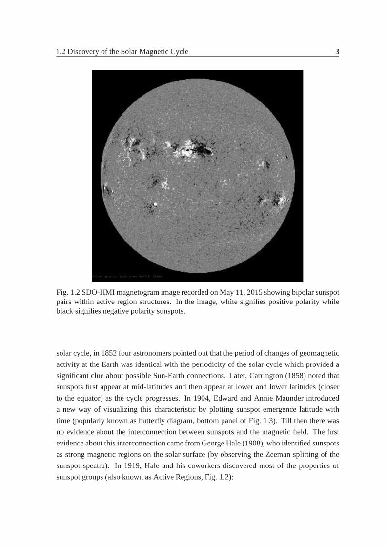
Fig. 1.2 SDO-HMI magnetogram image recorded on May 11, 2015 showing bipolar sunspotpairs within active region structures. In the image, white signifies positive polarity whileblack signifies negative polarity sunspots.
solar cycle, in 1852 four astronomers pointed out that the period of changes of geomagnetic
activity at the Earth was identical with the periodicity of the solar cycle which provided a
significant clue about possible Sun-Earth connections. Later, Carrington (1858) noted that
sunspots first appear at mid-latitudes and then appear at lower and lower latitudes (closer
to the equator) as the cycle progresses. In 1904, Edward and Annie Maunder introduced
a new way of visualizing this characteristic by plotting sunspot emergence latitude with
time (popularly known as butterfly diagram, bottom panel of Fig. 1.3). Till then there was
no evidence about the interconnection between sunspots andthe magnetic field. The first
evidence about this interconnection came from George Hale (1908), who identified sunspots
as strong magnetic regions on the solar surface (by observing the Zeeman splitting of the
sunspot spectra). In 1919, Hale and his coworkers discovered most of the properties of
sunspot groups (also known as Active Regions, Fig. 1.2):
4 Introduction to the Solar Magnetic Cycle
1700 1750 1800 1850 1900 1950 20000
20
40
60
80
100
120
140
160
180
200
Time (years)
Sun
spot
Num
ber
Fig. 1.3 Top panel: Plot of international sunspot number as afunction of time in years.Bottom panel: Latitude vs time plot from recent high resolution observations. Backgroundshows weak, diffuse radial field on the photosphere. This plot is widely known as thebutterfly diagram. Image credit: Hathaway/NASA/MSFC.
• Sunspots frequently appear in pairs at the surface and the relative orientation of the
magnetic field of most active regions is opposite across the equator.
• The polarity of active regions change from one to another solar cycle but remains same
in a hemisphere for a given solar cycle.
• The line joining the bipolar sunspot pairs are tilted with respect to the east-west direc-
tion (leading spot along the direction of rotation is closerto the equator than the following
spot) and this tilt angle increases with latitude. This is known as Joy’s law.
Harold Babcock and his son Horace Babcock (1955) developed the magnetograph and
used this magnetograph to study the distribution of magnetic fields on the region outside of
sunspots. A very weak field of the order of 10 Gauss was found tobe mostly concentrated
1.3 Generation of the Large Scale Solar Magnetic Field 5
in the latitude above 55, (Babcock, 1959). This weak diffuse magnetic field migrates
poleward and changes the sign of the polar field every 11 years. Note that the polar field
reverses its polarity when the sunspot number is maximum. Wealso note that recent high
resolution observations find vertically oriented magneticflux tubes with strong kilo-Gauss
magnetic field strength in the polar region (Tsuneta et al. 2008), which might also contribute
to the polar field.
There is also another type of photospheric magnetic field structure known as small scale
magnetic field. This mixed polarity small scale magnetic field is very dynamic and does
not vary much with the solar cycle. Although the origin of this small scale magnetic field
is unknown, some recent studies suggest that a small scale dynamo near the solar surface
(local dynamo), may be the source for this small scale magnetic field (Petrovay & Szakaly
1993; Cattaneo 1999; Danilovic et al. 2010; Lites 2011).
1.3 Generation of the Large Scale Solar Magnetic Field
1.3.1 Magnetohydrodynamics
Matter inside the Sun exists in the ionized (plasma) state. To explain the magnetic nature
of the solar cycle, one has to understand the behaviour of magnetic fields inside electrically
conducting fluids – which is the heart of the subject Magnetohydrodynamics (MHD). The
interaction of the plasma velocity field with the magnetic field can be described through the
magnetic induction equation:
∂B∂ t
= ∇× (v×B)+λ∇2B, (1.1)
where the first term in the right hand side of the equation is the source term and the second
term is the diffusion term. Here we assume the situation where the diffusivity (λ ) does not
vary with space.
One important input in the induction equation is the velocity (v). To describe a MHD
system self-consistently, we also require the Navier-Stokes equation, which describes the
evolution of the velocity field.
ρ∂v∂ t
+ρ(v ·∇)v =−∇p+J×B+ρg+∇.τ, (1.2)
wherev is the fluid velocity,−∇p is the force due to pressure gradient,J×B is the Lorentz
force term andτ is the viscous stress tensor. The Lorentz force term is calculated using
6 Introduction to the Solar Magnetic Cycle
the solution of induction equation (B), which acts as a forcing term in the Navier-Stokes
equation.
Note thatB = 0 is a valid solution of the induction equation, so that no magnetic field
generation is possible if we start with zero magnetic field. So there must be some mechanism
through which initial seed magnetic fields can be generated and amplified. As we are mainly
interested in the generation of large scale solar magnetic fields, it is suffice to assume that
we start with a pre-existing seed magnetic field. Dynamo is a process which can amplify
this seed magnetic field to produce large scale magnetic fields by converting the kinetic
energy of plasma into magnetic energy. So, in order to explore the full dynamical behaviour
of the magnetized plasma, we have to solve equations (1.1), (1.2) together with the mass
continuity and energy conservation equations:
∂ρ∂ t
+∇.(ρv) = 0, (1.3)
∂ p∂ t
+v.∇p+ γ p∇.v =−(γ −1)L, (1.4)
whereL is the heat loss rate which consists of the terms due to thermal conduction, ohmic
heating etc. andγ represents the ratio between specific heats. These equations along with
∇.B= 0 and equation of state, comprise the full set of MHD equations.
The evolution of magnetic field (equation 1.1) inside the plasma is governed by the
competition between induction and diffusion of the magnetic field. If we take the ratio of
two terms on the right hand side of the equation then we get themagnetic Reynold’s number,
Rm = VLη whereV is the velocity andL is the spatial length-scale. Now it is obvious that
Rm ≫ 1 for astrophysical systems as length scales (L) are very large. In this case one may
approximate the induction equation as:
∂B∂ t
≃ ∇× (v×B). (1.5)
In this situation (i.e., in the ideal MHD limit), Alfvén (1942a) pointed out that magnetic flux
is conserved inside the plasma system and moves with the fluid. This theorem is known as
Alfvén’s theorem of flux-freezing. It is well known from early nineteenth century observa-
tions that the Sun rotates differentially with the equator rotating faster than the pole. Since
the flux is frozen inside the plasma, it allows differential rotation to stretch magnetic field
lines along the direction of rotation (i.e., the toroidal orφ direction). This process is known
as theΩ-effect and was first pointed out by Larmor (1919).
1.3 Generation of the Large Scale Solar Magnetic Field 7
Theoretical and numerical magnetoconvection studies performed by Chandrasekhar (1952)
and Weiss (1981) suggest that in the presence of magnetic field, convective systems get sep-
arated into regions that are free of magnetic field where vigorous convection takes place
while magnetic fields are concentrated into thin structuresin the form of flux tubes. It is
also known that the presence of strong magnetic field makes the magneto-fluid more stable
against convection, i.e., convection is suppressed withinregions of strong magnetic field due
to the tension of magnetic field lines (Thompson 1951; Chandrasekhar 1952). Since convec-
tion is suppressed in regions of strong magnetic field, thereis less efficient heat transport in
these regions. Because of this, sunspots appear darker thanthe surroundings. To sum up, it
is expected that magnetic field exists in the form of flux tubesinside the solar convection
zone and strong differential rotation of the Sun stretches these flux tubes in the toroidal i.e.,
φ -direction.
Let us assume that the gas pressure inside the flux tube ispint and outside it ispext, B is
the strength of magnetic field inside the flux tube. To maintain pressure balance across the
surrounding surface of the flux tube:
pext = pint +B2
2µ0. (1.6)
When the flux tubes are in isothermal condition, the above equation implies,ρext ≥ ρint . If
such a situation arises in any part of the flux tube, then this part will experience a buoyancy
force. Due to magnetic buoyancy this part rises up against gravity and generates bipolar
sunspot pairs on the solar surface (Parker 1955a, 1955b).
1.3.2 Parker’s Mean-Field Dynamo
In spherical geometry, we can write the magnetic field as:
B = Br r +Bθ θ +Bφ φ . (1.7)
We consider the stellar system as axisymmetric with the rotation axis coinciding with the
axis of symmetry. ThenBr , Bθ andBφ do not vary withφ . In this situation, we can write
the magnetic field as a sum of the toroidal (Bt) and poloidal (Bp) field components.
B = Bt +Bp, (1.8)
whereBt = Bφ φ andBp = Br r +Bθ θ .
8 Introduction to the Solar Magnetic Cycle
(a) (b)
Fig. 1.4 Parker’s turbulent dynamo: (a) Theω-effect: Poloidal field lines are stretched bydifferential rotation in the solar interior and produces the toroidal component of magneticfield. (b) α-effect: At the time of rise through the convection zone, toroidal flux tubes aretwisted due to helical turbulence and produces magnetic field components in the poloidalplane. Image credit: Hathaway/NASA/MSFC
In this case,Bp can be expressed in terms of the vector potential:
Bp = ∇×Aφ . (1.9)
To explain the origin of the solar cycle, Parker (1955b) firstproposed the idea of flux
recycling between the toroidal and poloidal field components.
The first part of the full dynamo mechanism (Poloidal→ Toroidal) relies on the idea
proposed by Larmor (1919). In this process shearing of the large scale poloidal field due to
strong differential rotation produces the toroidal field.
The second part of the dynamo mechanism (Toroidal→ Poloidal) is a debated issue.
The first breakthrough in this direction was proposed by Parker (1955b). The idea was that
when some part of the toroidal flux tube rises through the convection zone due to mag-
netic buoyancy, they are subject to helical turbulence which imparts a twist to the rising
plasma blobs. As magnetic field is frozen inside the plasma, this helical twist of plasma
blobs also imparts a helical twist to the magnetic field. Thusrising toroidal flux tubes are
helically twisted out of the plane and produce magnetic fieldcomponent in the poloidal
plane. Although the idea of Parker at that time was largely intuitive, it was put on rigorous
1.3 Generation of the Large Scale Solar Magnetic Field 9
mathematical footing after a decade through the development of mean field electrodynamics
(Steenbeck, Krause & Rädler 1966).
1.3.3 Mean Field Electrodynamics
Turbulence is expected to play an important role in the solardynamo as the solar convective
zone is highly turbulent. As it is not possible to develop a deterministic theory to tackle
turbulence, it is necessary to develop a statistical schemebased on average properties of
turbulence.
In a turbulent medium, we can decompose the fluid velocity (v) and magnetic field (B)
in terms of mean and fluctuating parts. Thus:
v = v+v′, B = B+B′ (1.10)
where the term with overline corresponds to the mean and the primed terms correspond to
the fluctuating parts. In mean field theory the mean typicallydenotes ensemble averages
over length-scales and time-scales much larger than turbulent eddy length-scale and eddy
turn over time scales. Also by definition,v′ = B′ = 0, i.e., mean of the fluctuating compo-
nents are zero. Substituting (1.10) into the magnetic induction equation (1.1) we get:
∂ B∂ t
+∂B′
∂ t= ∇× (v× B+v′× B+ v×B′+v′×B′)+λ∇2(B+B′), (1.11)
where diffusivity (λ ) is constant. Again averaging equation (1.11) term by term,we get:
∂ B∂ t
= ∇× (v× B)+∇× ε +λ∇2(B+B′), (1.12)
whereε = v′×B′ is known as the mean electromotive force which arises because of the cor-
relation between fluctuating components of velocity and magnetic fields (Steenbeck, Krause
& Rädler 1966; Krause & Rädler 1980). Subtracting (1.12) from (1.11), we get
∂B′
∂ t= ∇× (v′× B+ v×B′+v′×B′− ε)+λ∇2B′. (1.13)
Let us assume at initial time (t = 0), fluctuation in the magnetic field is zero. From equation
(1.13), it is clear that if there is no fluctuation in the magnetic field (B′ = 0) then there is a
linear relationship between mean electromotive force (ε) and mean magnetic field (B). Now
if we assume that the spatial scale of the fluctuation is very small compared to the mean
10 Introduction to the Solar Magnetic Cycle
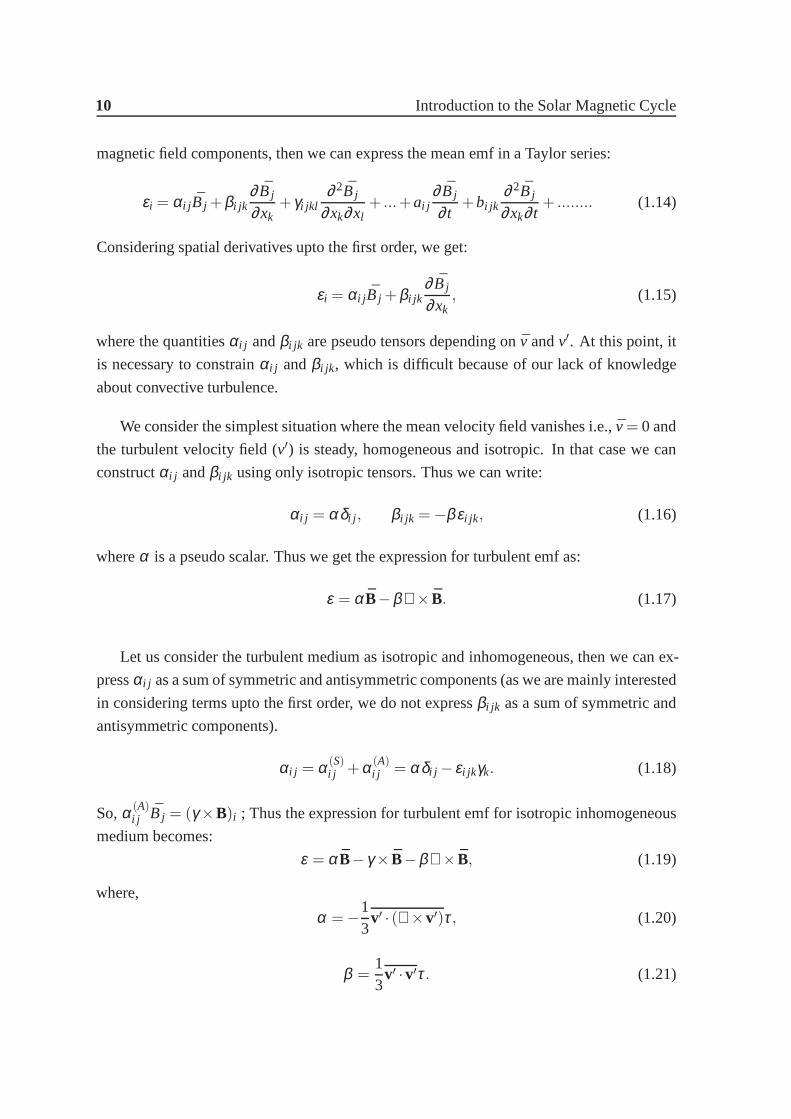
magnetic field components, then we can express the mean emf ina Taylor series:
εi = αi j B j +βi jk∂ B j
∂xk+ γi jkl
∂ 2B j
∂xk∂xl+ ...+ai j
∂ B j
∂ t+bi jk
∂ 2B j
∂xk∂ t+ ........ (1.14)
Considering spatial derivatives upto the first order, we get:
εi = αi j B j +βi jk∂ B j
∂xk, (1.15)
where the quantitiesαi j andβi jk are pseudo tensors depending on ¯v andv′. At this point, it
is necessary to constrainαi j andβi jk , which is difficult because of our lack of knowledge
about convective turbulence.
We consider the simplest situation where the mean velocity field vanishes i.e., ¯v= 0 and
the turbulent velocity field (v′) is steady, homogeneous and isotropic. In that case we can
constructαi j andβi jk using only isotropic tensors. Thus we can write:
αi j = αδi j , βi jk =−βεi jk , (1.16)
whereα is a pseudo scalar. Thus we get the expression for turbulent emf as:
ε = αB−β∇× B. (1.17)
Let us consider the turbulent medium as isotropic and inhomogeneous, then we can ex-
pressαi j as a sum of symmetric and antisymmetric components (as we aremainly interested
in considering terms upto the first order, we do not expressβi jk as a sum of symmetric and
antisymmetric components).
αi j = α(S)i j +α(A)
i j = αδi j − εi jkγk. (1.18)
So,α(A)i j B j = (γ ×B)i ; Thus the expression for turbulent emf for isotropic inhomogeneous
medium becomes:
ε = αB− γ × B−β∇× B, (1.19)
where,
α =−13
v′ · (∇×v′)τ, (1.20)
β =13
v′ ·v′τ. (1.21)
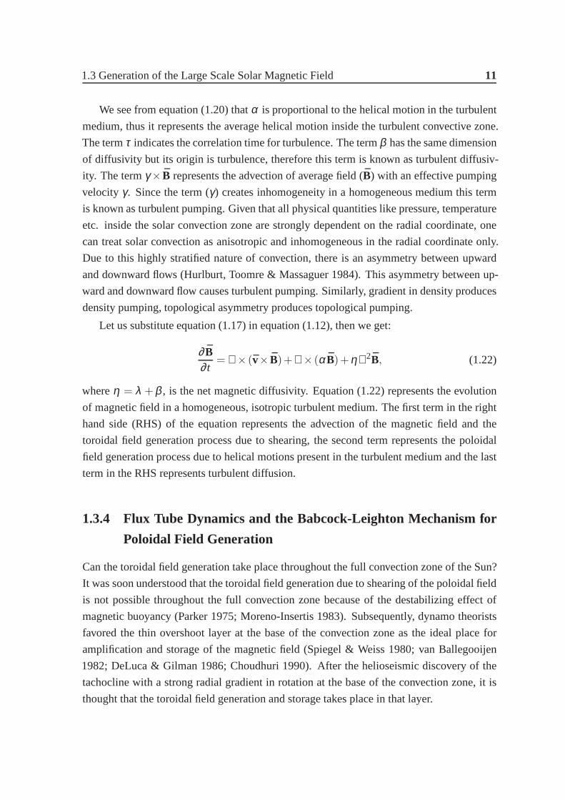
1.3 Generation of the Large Scale Solar Magnetic Field 11
We see from equation (1.20) thatα is proportional to the helical motion in the turbulent
medium, thus it represents the average helical motion inside the turbulent convective zone.
The termτ indicates the correlation time for turbulence. The termβ has the same dimension
of diffusivity but its origin is turbulence, therefore thisterm is known as turbulent diffusiv-
ity. The termγ × B represents the advection of average field (B) with an effective pumping
velocity γ. Since the term (γ) creates inhomogeneity in a homogeneous medium this term
is known as turbulent pumping. Given that all physical quantities like pressure, temperature
etc. inside the solar convection zone are strongly dependent on the radial coordinate, one
can treat solar convection as anisotropic and inhomogeneous in the radial coordinate only.
Due to this highly stratified nature of convection, there is an asymmetry between upward
and downward flows (Hurlburt, Toomre & Massaguer 1984). Thisasymmetry between up-
ward and downward flow causes turbulent pumping. Similarly,gradient in density produces
density pumping, topological asymmetry produces topological pumping.
Let us substitute equation (1.17) in equation (1.12), then we get:
∂ B∂ t
= ∇× (v× B)+∇× (αB)+η∇2B, (1.22)
whereη = λ +β , is the net magnetic diffusivity. Equation (1.22) represents the evolution
of magnetic field in a homogeneous, isotropic turbulent medium. The first term in the right
hand side (RHS) of the equation represents the advection of the magnetic field and the
toroidal field generation process due to shearing, the second term represents the poloidal
field generation process due to helical motions present in the turbulent medium and the last
term in the RHS represents turbulent diffusion.
1.3.4 Flux Tube Dynamics and the Babcock-Leighton Mechanism for
Poloidal Field Generation
Can the toroidal field generation take place throughout the full convection zone of the Sun?
It was soon understood that the toroidal field generation dueto shearing of the poloidal field
is not possible throughout the full convection zone becauseof the destabilizing effect of
magnetic buoyancy (Parker 1975; Moreno-Insertis 1983). Subsequently, dynamo theorists
favored the thin overshoot layer at the base of the convection zone as the ideal place for
amplification and storage of the magnetic field (Spiegel & Weiss 1980; van Ballegooijen
1982; DeLuca & Gilman 1986; Choudhuri 1990). After the helioseismic discovery of the
tachocline with a strong radial gradient in rotation at the base of the convection zone, it is
thought that the toroidal field generation and storage takesplace in that layer.
12 Introduction to the Solar Magnetic Cycle
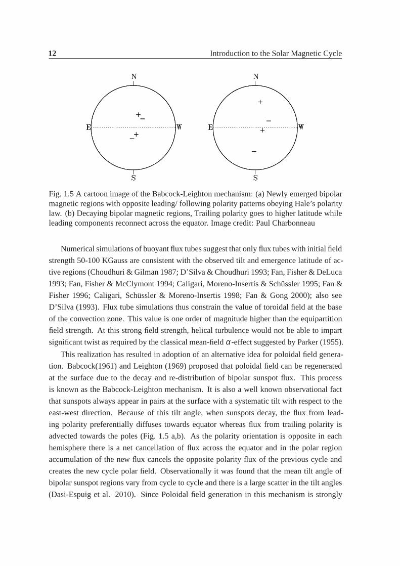
Fig. 1.5 A cartoon image of the Babcock-Leighton mechanism:(a) Newly emerged bipolarmagnetic regions with opposite leading/ following polarity patterns obeying Hale’s polaritylaw. (b) Decaying bipolar magnetic regions, Trailing polarity goes to higher latitude whileleading components reconnect across the equator. Image credit: Paul Charbonneau
Numerical simulations of buoyant flux tubes suggest that only flux tubes with initial field
strength 50-100 KGauss are consistent with the observed tilt and emergence latitude of ac-
tive regions (Choudhuri & Gilman 1987; D’Silva & Choudhuri 1993; Fan, Fisher & DeLuca
1993; Fan, Fisher & McClymont 1994; Caligari, Moreno-Insertis & Schüssler 1995; Fan &
Fisher 1996; Caligari, Schüssler & Moreno-Insertis 1998; Fan & Gong 2000); also see
D’Silva (1993). Flux tube simulations thus constrain the value of toroidal field at the base
of the convection zone. This value is one order of magnitude higher than the equipartition
field strength. At this strong field strength, helical turbulence would not be able to impart
significant twist as required by the classical mean-fieldα-effect suggested by Parker (1955).
This realization has resulted in adoption of an alternativeidea for poloidal field genera-
tion. Babcock(1961) and Leighton (1969) proposed that poloidal field can be regenerated
at the surface due to the decay and re-distribution of bipolar sunspot flux. This process
is known as the Babcock-Leighton mechanism. It is also a wellknown observational fact
that sunspots always appear in pairs at the surface with a systematic tilt with respect to the
east-west direction. Because of this tilt angle, when sunspots decay, the flux from lead-
ing polarity preferentially diffuses towards equator whereas flux from trailing polarity is
advected towards the poles (Fig. 1.5 a,b). As the polarity orientation is opposite in each
hemisphere there is a net cancellation of flux across the equator and in the polar region
accumulation of the new flux cancels the opposite polarity flux of the previous cycle and
creates the new cycle polar field. Observationally it was found that the mean tilt angle of
bipolar sunspot regions vary from cycle to cycle and there isa large scatter in the tilt angles
(Dasi-Espuig et al. 2010). Since Poloidal field generation in this mechanism is strongly
1.3 Generation of the Large Scale Solar Magnetic Field 13
dependent on the tilt angle of the bipolar sunspot pairs, this mechanism itself is a source of
irregularity (Choudhuri et al. 2007; Jiang et al. 2007). Recent observational results also
lend strong support to this mechanism (Dasi-Espuig et al. 2010; Kitchatinov & Olemskoy
2011a; Muñoz-Jaramillo et al. 2013). In recent years most ofthe kinematic dynamo models
are based on the scenario that – a) The toroidal field is produced due to strong differential
rotation in the convection zone b) The poloidal field is produced near the solar surface due
to decay of bipolar sunspot regions.
1.3.5 Differential Rotation and Meridional Circulation: E ssential In-
gredients of Solar Dynamo Modelling
In his classic paper, Parker (1955) showed that linear dynamo equations support periodically
propagating dynamo wave solutions – which signifies the solar cycle. The direction of such
periodic propagating dynamo waves is given by:
s= α∇Ω× φ , (1.23)
whereΩ is the solar differential rotation which arises mainly because of Reynolds stresses
< vrvθ > and< vθ vφ > (which creates angular momentum flux). To obtain the equatorward
propagation of dynamo waves (in keeping with the equatorward migration of the sunspot
belt), the following condition must be satisfied:
α∂Ω∂ r
< 0. (1.24)
This is known as the Parker-Yoshimura sign rule (Parker 1955; Yoshimura 1975). Since
at that time the profile of the differential rotation inside the convection zone was unknown,
there was full freedom to choose the profile of differential rotation such that results match
with observation. When the differential rotation was measured by helioseismology with
great accuracy (Thompson et al. 1996; Kosovichev et al. 1997; Schou et al. 1998) it was
found that the observed differential rotation profile wouldgive rise to poleward propagating
dynamo solutions as there is a negative radial shear at low latitudes. At this point it was
necessary to address this problem.
Observations of small magnetic features on the solar surface show that they are car-
ried by surface flows from equator to pole with an estimated speed of 10-20 m/s (Komm,
Howard & Harvey 1993; Latushko 1994; Snodgrass & Dailey 1996; Hathaway 1996). This
axisymmetric poleward flow in the meridional plane is known as meridional circulation.
Helioseismic measurements in later time also confirmed these observations and measured
14 Introduction to the Solar Magnetic Cycle
these poleward flows more accurately at the top 10 % of the solar convection zone (Giles
et al. 1997; Schou & Bogart 1998; Braun & Fan 1998, González Hernández et al. 1999).
Although measurement of the meridional circulation deep inthe convection zone is still not
possible, it is reasonable to assume that there must be an equatorward return flow some-
where in the convection zone because of mass conservation. The latitudinal structure of
the surface meridional flow is well observed (Hathaway & Rightmire 2010,2011; Hathaway
1996) but the radial structure still remains largely controversial (Zhao et al. 2013). If these
two largely segregated source layers (α-effect is at the surface whileΩ-effect is at the base
of the convection zone) are only coupled by diffusion (no meridional circulation is present),
then there is poleward propagation of the sunspot belt according to the Parker-Yoshimura
sign rule. However if these two layers are coupled by meridional circulation then we can get
equatorward propagation of sunspot belts even if the Parker-Yoshimura sign rule is violated
(Choudhuri et al. 1995; Durney 1995). After this insight meridional circulation became an
essential ingredient in solar dynamo models.
1.3.6 Kinematic Babcock-Leighton Dynamo Models
In the kinematic dynamo problem, plasma flows are taken as inputs and it is assumed that
the mean flows are not significantly altered by the Lorentz force. Observationally it is found
that mean flows do not vary significantly with time thus the kinematic approach may be a
good approximation to study the evolution of solar magneticfields. In the axisymmetric
spherical coordinate system, we can represent the magneticand velocity fields as:
B(r,θ , t) = ∇× (A(r,θ , t)φ)+B(r,θ , t)φ, v = r sin(θ)Ωφ +vp, (1.25)
whereB(r,θ , t) andA(r,θ , t) represents the toroidal magnetic field and vector potentialfor
the poloidal magnetic field,Ω is the differential rotation andvp is the meridional flow.
Substituting these into the magnetic induction equation, we get the standardαω -dynamo
equations:∂A∂ t
+1s[vp ·∇(sA)] = η
(∇2− 1
s2
)A+S(r,θ ,B), (1.26)
∂B∂ t
+s
[vp ·∇
(Bs
)]+(∇ ·vp)B= η
(∇2− 1
s2
)B+s
([∇× (Aeφ )
]·∇Ω
)+
1s
∂ (sB)∂ r
∂η∂ r
,
(1.27)
wheres= r sin(θ). The terms withvp in left hand side of both the equations correspond
to the advection and deformation of magnetic field by meridional circulation. In the right
hand side of both the equations, first term corresponds to thediffusion of magnetic field
1.3 Generation of the Large Scale Solar Magnetic Field 15
0.5 0.55 0.6 0.65 0.7 0.75 0.8 0.85 0.9 0.95 110
8
109
1010
1011
1012
1013
r/R0
η (c
m2 /s
)
(a) (b)
Fig. 1.6 (a) Variation of turbulent magnetic diffusivity diffusivity with radius. (b) Analyticaldifferential rotation profile (in nHz) used in dynamo model.Region between two dashedcircular arcs indicates the tachocline.
and second term corresponds to the source term. On the RHS of equation (1.27), the third
term corresponds to the advection of magnetic field due to thegradient of turbulent diffu-
sivity. In equation (1.26),S(r,θ ,B) represents the generation of poloidal field due to the
Babcock-Leighton mechanism. For the research work described in this thesis, we model the
Babcock-Leighton mechanism i.e., the source term for poloidal field evolution equation by
the methods of double ring proposed by Durney (1997) and subsequently used by Nandy &
Choudhuri (2001), Muñoz-Jaramillo, Nandy, Martens & Yeates (2010) and Nandy, Muñoz-
Jaramillo & Martens (2011). In equation (1.26) and (1.27), we have to define three input
ingredients so that we can solve these system of equations: magnetic diffusivity, differential
rotation and meridional circulation.
Now we discuss these three essential input ingredients in kinematic solar dynamo mod-
els, namely, turbulent diffusivity, differential rotation and meridional circulation. With the
turbulent diffusivity term we try to capture the net effect of convective turbulence on the
large scale magnetic field. This term also acts as a communicator between two source lay-
ers (as two source layers are segregated; the poloidal field generation takes place at the solar
surface while the toroidal field generation takes place at the base of the convection zone).
Here we use double step diffusivity profile (Dikpati et al. 2002; Chatterjee, Nandy & Choud-
huri 2004; Guerrero & de Gouveia Dal Pino 2007; Jouve & Brun 2007, Muñoz-Jaramillo,
16 Introduction to the Solar Magnetic Cycle
Nandy & Martens 2009):
η(r) = ηbcd+ηcz−ηbcd
2
(1+erf
(r − rcz
dcz
))
+ηsg−ηcz−ηbcd
2
(1+erf
(r − rsg
dsg,
)). (1.28)
whereηbcd = 108 cm2/s,ηcz= 1011 cm2/s andηsg= 5×1012 cm2/s corresponds to the dif-
fusivity at the bottom of computational domain, diffusivity in the convection zone and near
surface supergranular diffusivity respectively. Transition from one value of diffusivity to
another is characterized byrcz= 0.73R⊙, dcz= 0.015R⊙, rsg= 0.95R⊙ anddsg= 0.015R⊙.
The typical double step magnetic diffusivity profile is shown in Fig. 1.6 (a). See Muñoz-
Jaramillo et al. (2011) for a discussion on constraining thediffusivity profile.
One necessary input parameter in solar dynamo models is the differential rotation (vφ ;
which stretches poloidal field lines in theφ -direction and creates the toroidal field). Here
we use the differential rotation profile as prescribed by Muñoz-Jaramillo et al. (2009) (see
Fig. 1.6 (b)):
ΩA(r,θ) = 2πΩc+π2
(1−erf
(r−rtcdtc
))(Ωe−Ωc+(Ωp−Ωe)ΩS(θ)) ,
ΩS(θ) = acos2(θ)+(1−a)cos4(θ),
(1.29)
wherertc = 0.7R⊙ i.e. the location of the tachocline,dtc = 0.025R⊙ i.e. half of thickness of
the tachocline,Ωc = 432 nHz i.e. rotation frequency of the core,Ωe= 470 nHz i.e. rotation
frequency of the equator,Ωp = 330 nHz i.e. rotation frequency of the pole anda= 0.483.
The meridional circulation (i.e., velocity component in the r −θ plane) can be defined
as
vp (r,θ) =1
ρ(r)∇×
(ψ(r,θ)eφ
). (1.30)
which is estimated from the stream function (defined within 0≤ θ ≤ π/2, i.e., in the north-
ern hemisphere) as described in Chatterjee, Nandy and Choudhuri (2004):
ψr sinθ = ψ0(r −Rp)sin
[π(r −Rp)
(R⊙−Rp)
]1−e−β1θ ε
1−eβ2(θ−π/2)e−((r−r0)/Γ)2, (1.31)
where the parameters are defined as follow:β1 = 1.5, β2 = 1.8, ε = 2.0000001, r0 =
(R⊙−Rb)/4, Γ = 3.47×10⁸ m. The termψ0 determines the the maximum speed of the
flow. Rp is the penetration depth of the meridional flow. The meridional circulation profile
1.3 Generation of the Large Scale Solar Magnetic Field 17
0.55 0.6 0.65 0.7 0.75 0.8 0.85 0.9 0.95 1−18
−16
−14
−12
−10
−8
−6
−4
−2
0
2
r/Ro
v θ (m
s−
1 )
(a) (b)
Fig. 1.7 (a) Meridional circulation streamlines used in ourmodel. Region between twodashed circular arcs indicates the tachocline. (b) Plot of latitudinal velocity (vθ in m/s) as afunction ofr/R0 at 450 latitude.
−80 −60 −40 −20 0 20 40 60 80−20
−15
−10
−5
0
5
10
15
20
θ (in o)
v θ (m
s−
1 )
Fig. 1.8 Plot of latitudinal velocity (vθ in m/s) as a function of latitude (θ ) at the solarsurface.
in the southern hemisphere is generated by a mirror reflection of the velocity profile across
the equator. Streamlines of a typical meridional circulation profile are shown in Fig. 1.7 (a).
Taking the density stratification in the convection zone asρ = C(R⊙r − γ)m (from stan-
dard solar model; Christensen-Dalsgaard et al. 1996), we get the speed of meridional circu-
lation:
vr =1
ρr2sinθ∂
∂θ(ψr sinθ), (1.32)
18 Introduction to the Solar Magnetic Cycle
Time (years)
Latit
ude
150 160 170 180 190 200
−80
−60
−40
−20
0
20
40
60
80
Fig. 1.9 Butterfly diagram obtained from our flux transport dynamo model where back-ground shows weak diffuse radial field on solar surface and eruption latitudes are denotedby symbols black (“+”) and red (“+”), indicating underlyingnegative and positive toroidalfield respectively.
vθ =− 1ρr sinθ
∂∂ r
(ψr sinθ), (1.33)
where,γ = 0.95,m= 3/2.
Some studies find the peak speed of the flow is in the range of 12-20 m/s (Komm,
Howard & Harvey 1993; Braun & Fan 1998; Gizon & Rempel 2008). Here we set the
peak speed of the meridional circulation at mid latitudes tobe 18 m/s. Fig. 1.7 (b) shows
the variation of theθ component of this velocity at mid latitude as a function of solar radius.
Fig. 1.8 shows the variation of theθ component of this velocity as a function of latitude at
the solar surface.
Having defined all the input ingredients we can solve equations (1.26) and (1.27) with
appropriate boundary conditions. We perform all of our spatially extended dynamo simula-
tions in a meridional slab 0.55R⊙ < r <R⊙ and within 0< θ < π . Since we use axisymmet-
ric equations, both the poloidal and toroidal field vectors need to be zero (A= 0 andB= 0)
at the pole (θ = 0 andθ = π), to avoid any singularity. At the bottom of the computational
domain i.e., atr = 0.55R⊙, we assume perfectly conducting material, thus both field com-
ponents vanish (A= 0 andB= 0) at the bottom boundary. At the top (r = R⊙), we assume
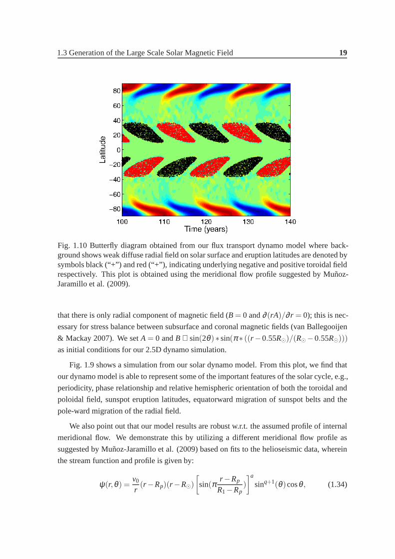
1.3 Generation of the Large Scale Solar Magnetic Field 19
Fig. 1.10 Butterfly diagram obtained from our flux transport dynamo model where back-ground shows weak diffuse radial field on solar surface and eruption latitudes are denoted bysymbols black (“+”) and red (“+”), indicating underlying negative and positive toroidal fieldrespectively. This plot is obtained using the meridional flow profile suggested by Muñoz-Jaramillo et al. (2009).
that there is only radial component of magnetic field (B= 0 and∂ (rA)/∂ r = 0); this is nec-
essary for stress balance between subsurface and coronal magnetic fields (van Ballegooijen
& Mackay 2007). We setA= 0 andB ∝ sin(2θ) ∗ sin(π ∗ ((r −0.55R⊙)/(R⊙−0.55R⊙)))as initial conditions for our 2.5D dynamo simulation.
Fig. 1.9 shows a simulation from our solar dynamo model. Fromthis plot, we find that
our dynamo model is able to represent some of the important features of the solar cycle, e.g.,
periodicity, phase relationship and relative hemisphericorientation of both the toroidal and
poloidal field, sunspot eruption latitudes, equatorward migration of sunspot belts and the
pole-ward migration of the radial field.
We also point out that our model results are robust w.r.t. theassumed profile of internal
meridional flow. We demonstrate this by utilizing a different meridional flow profile as
suggested by Muñoz-Jaramillo et al. (2009) based on fits to the helioseismic data, wherein
the stream function and profile is given by:
ψ(r,θ) =v0
r(r −Rp)(r −R⊙)
[sin(π
r −Rp
R1−Rp)
]a
sinq+1(θ)cosθ , (1.34)

20 Introduction to the Solar Magnetic Cycle
where, q=1 governs the latitudinal dependence,Rp=0.65R⊙ is the penetration depth, a=1.92
andR1 = 1.027R⊙ govern the location of the peak of poleward flow and the amplitude and
location of equatorward return flow.v0 = 18 is used to control the amplitude of meridional
flow. We find that the results do not change qualitatively withthe alternative meridional
flow profile (see Fig. 1.10).
In the next few chapters of this thesis, we will investigate some important features of the
solar cycle using this model.
Chapter 2
Exploring Grand Minima Phases with a
Low Order, Time Delay Dynamo Model
Fluctuations in the Sun’s magnetic activity, including episodes of grand minima such as
the Maunder minimum have important consequences for space and planetary environments.
However, the underlying dynamics of such extreme fluctuations remain ill-understood. In
this chapter we develop a low order time delay dynamo model removing all space de-
pendent terms. Introduction of time delays capture the physics of magnetic flux trans-
port between spatially segregated dynamo source regions inthe solar interior. We follow
the Babcock-Leighton approach to treat the poloidal field generation mechanism due to
decay and dispersal of tilted bipolar sunspot region. Introducing stochastic fluctuation
in Babcock-Leighton source term for poloidal field generation, we demonstrate that the
Babcock-Leighton poloidal field source based on dispersal of tilted bipolar sunspot flux,
alone, can not recover the sunspot cycle from a grand minimum. We find that an additional
poloidal field source effective on weak fields – e.g., the mean-field α-effect driven by he-
lical turbulence – is necessary for self-consistent recovery of the sunspot cycle from grand
minima episodes.
2.1 Introduction
Sunspots, which are strongly magnetized regions, play a keyrole in governing the activity
of the Sun. The number of sunspots observed on the solar surface waxes and wanes with
time generating the 11-year solar cycle. While there is a small variation in this periodicity,
fluctuations in the amplitude of the solar cycle are large. Extreme fluctuations are manifest
in grand maxima episodes – when the cycle amplitudes are muchhigher than normal, and
22 Exploring Grand Minima Phases with a Low Order, Time Delay Dynamo Model
grand minima episodes – when the cycle amplitudes fall drastically, even leading to the dis-
appearance of sunspots for an extended period of time. The most striking evidence of such
a minimum in the recorded history of sunspot numbers is the so-called Maunder minimum
between 1645 and 1715 AD (Eddy 1988). The lack of sunspots during this period is statis-
tically well-proven and is not due to the lack of observations – which covered 68% of the
days during this period (Hoyt & Schatten 1996). The occurrence of these solar activity ex-
tremes is correlated with temperature records over millennium scale (Usoskin et al. 2005);
the solar Maunder minimum coincided with the severest part of the Little Ice Age – a period
of global cooling on Earth.
Over the last decade, solar activity reconstructions basedon cosmogenic isotopes and
geomagnetic data (Usoskin et al. 2000, 2003, 2007; Miyaharaet al. 2004; Steinhilber et al.
2010; Lockwood & Owens 2011), which are indirect proxies forprobing long-term solar
activity have brought to the fore various properties of these grand minima episodes. These
observations show that there have been many such activity minima in the past; however the
solar cycle has recovered every time and regained normal activity levels. There is some
evidence for persistent, but very weak amplitude cycles during the Maunder minimum and
a slow strengthening of cycle amplitudes to normal levels during the recovery phase. While
the general perception was that the onset of the Maunder minimum was sudden, a recent
reconstruction based on historical sunspot records has challenged that notion indicating that
the onset phase of the minimum may have been gradual (Vaqueroet al. 2011).
A magnetohydrodynamic (MHD) dynamo mechanism, involving interactions of plasma
flows and magnetic fields drives the solar cycle. Our understanding of the solar dynamo,
see e.g., the reviews by Ossendrijver (Ossendrijver 2003) and Charbonneau (Charbonneau
2010), is based on the generation and recycling of the toroidal and poloidal components of
the Sun’s magnetic field. The toroidal magnetic field is produced by stretching of poloidal
field lines by differential rotation – a process termed as theΩ-effect (Parker 1955). It is
thought this process is concentrated near the base of the solar convection zone (SCZ) –
where the upper part of the tachocline (a region of strong radial gradient in the rotation)
and overshoot layer (which is stable to convection) offers an ideal location for toroidal field
amplification and storage. Sufficiently strong toroidal fluxtubes are magnetically buoyant
and erupt radially outwards producing sunspots where they intersect the solar surface.
For the dynamo to function, the poloidal component has to be regenerated back from the
toroidal component, a step for which, diverse propositionsexist. The first such proposition
invoked helical turbulent convection as a means of twistingrising toroidal flux tubes to
regenerate the poloidal component (a mechanism traditionally known as the the mean field
α-effect; Parker 1955). Numerous dynamo models based on the mean-fieldα-effect were
2.1 Introduction 23
constructed and such models enjoyed a long run as the leadingcontender for explaining
the origin of the solar cycle (Charbonneau 2010). However, subsequent simulations of
the dynamics of buoyant toroidal flux tubes and observational constraints set by the tilt
angle distribution of sunspots pointed out that the toroidal magnetic field at the base of the
SCZ must be as high as 105 G (D’Silva & Choudhuri 1993; Fan et al. 1993; Caligari et
al. 1995); such strong toroidal flux tubes being one order of magnitude stronger than the
equipartition magnetic field in the SCZ would render the meanfield α-effect ineffective.
This consideration revived interest in an alternative mechanism of poloidal field production
based on the flux transport mediated decay and dispersal of tilted bipolar sunspots pairs in
the near-surface layers (Babcock 1961; Leighton 1969), hereby, referred to as the Babcock-
Leighton mechanism.
In the last couple of decades, multiple dynamo models have been based on this idea
(Durney 1997; Dikpati & Charbonneau 1999; Nandy & Choudhuri2002; Chatterjee et al.
2004; Muñoz-Jaramillo et al. 2009) and have successfully reproduced many nuances of the
solar cycle. Some (Tobias et al. 2006; Bushby & Tobias 2007; Cattaneo & Hughes 2009)
have criticised the usage of such mean-field dynamo models topredict the solar cycle, how-
ever it should be noted that recent studies (Simard et al. 2013; Dube & Charbonneau 2013)
indicate that if input profiles are extracted from three-dimensional full MHD simulations
and fed into two-dimensional mean-field dynamo models, theyare capable of producing
qualitatively similar solutions to those found in the full MHD simulations. The major ad-
vantage of the mean-field dynamo framework is that it allows for much faster integration
times compared to the full MHD simulations and are thereforecomputationally efficient as
well as physically transparent. Recent observations also lend strong support to the Babcock-
Leighton mechanism (Dasi-Espuig et al. 2010; Muñoz-Jaramillo et al. 2013) and this is now
believed to be the dominant source for the Sun’s poloidal field. Surface transport models
(Wang et al. 1989; van Ballegooijen et al. 2010) also providetheoretical evidence that this
mechanism is in fact operating in the solar surface. Randomness or stochastic fluctuations
in the Babcock-Leighton poloidal field generation mechanism is an established method for
exploring variability in solar cycle amplitudes (Charbonneau & Dikpati 2000; Charbonneau
et al. 2004, 2005; Passos & Lopes 2011; Passos et al. 2012, Choudhuri & Karak 2012) as
are deterministic or non-linear feedback mechanisms (Wilmot-Smith et al. 2005; Jouve et
al. 2010). Stochastic fluctuations within the dynamo framework are physically motivated
from the random buffeting that a rising magnetic flux tube endures during its ascent through
the turbulent convection zone and from the observed scatteraround the mean (Joy’s law)
distribution of tilt angles. It is to be noted that similar fluctuations are to be expected in the
24 Exploring Grand Minima Phases with a Low Order, Time Delay Dynamo Model
mean-fieldα effect as well (Hoyng 1988) and such phenomenon can be explored within the
framework of truncated mean-field dynamo models (Yoshimura1975).
Since the two source layers for toroidal field generation (theΩ effect) and poloidal field
regeneration (theα-effect) are spatially segregated in the SCZ, there must be effective com-
munication to complete the dynamo loop. Magnetic buoyancy efficiently transports toroidal
field from the bottom of the convection zone to the solar surface. On the other hand, merid-
ional circulation, turbulent diffusion and turbulent pumping share the role of transporting
the poloidal flux from the surface back to the solar interior (Karak & Nandy 2012) where
the toroidal field of the next cycle is generated thus keepingthe cycles going. Thus, there is
a time delay built into the system due to the finite time required for transporting magnetic
fluxes from one source region to another within the SCZ.
Based on delay differential equations and the introductionof randomness on the poloidal
field source, here we construct a novel, stochastically forced, non-linear time delay dynamo
model for the solar cycle to explore long-term solar activity variations. We particularly fo-
cus our investigations on the recovery from grand minima phases and demonstrate that the
Babcock-Leighton mechanism alone – which is believed to be the dominant source for the
poloidal field – cannot restart the solar cycle once it settles into a prolonged grand minimum.
The presence of an additional poloidal field source capable of working on weak magnetic
fields, such as the mean fieldα-effect is necessary for recovering the solar cycle.
2.2 Stochastically Forced, Non-Linear, Time Delay Solar
Dynamo Model
The model is an extension of the low order time delay dynamo equations previously explored
by Wilmot-Smith et al. (2006). This model was derived considering only the source and
dissipative mechanisms in the dynamo process. All space dependent terms were removed
and instead the physical effect of flux transport through space was captured through the
explicit introduction of time delays in the system of equations.
The time delay dynamo equations are given by
dBφ (t)
dt=
ωL
A(t−T0)−Bφ (t)
τ(2.1)
dA(t)dt
= α0 f1(Bφ (t −T1))Bφ (t−T1)−A(t)
τ, (2.2)
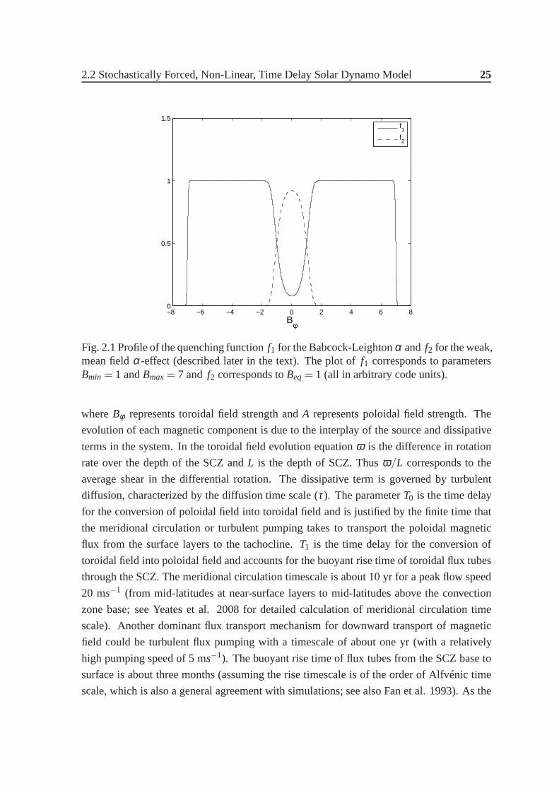
2.2 Stochastically Forced, Non-Linear, Time Delay Solar Dynamo Model 25
−8 −6 −4 −2 0 2 4 6 80
0.5
1
1.5
Bφ
f1
f2
Fig. 2.1 Profile of the quenching functionf1 for the Babcock-Leightonα and f2 for the weak,mean fieldα-effect (described later in the text). The plot off1 corresponds to parametersBmin = 1 andBmax= 7 and f2 corresponds toBeq= 1 (all in arbitrary code units).
whereBφ represents toroidal field strength andA represents poloidal field strength. The
evolution of each magnetic component is due to the interplayof the source and dissipative
terms in the system. In the toroidal field evolution equationω is the difference in rotation
rate over the depth of the SCZ andL is the depth of SCZ. Thusω/L corresponds to the
average shear in the differential rotation. The dissipative term is governed by turbulent
diffusion, characterized by the diffusion time scale (τ). The parameterT0 is the time delay
for the conversion of poloidal field into toroidal field and isjustified by the finite time that
the meridional circulation or turbulent pumping takes to transport the poloidal magnetic
flux from the surface layers to the tachocline.T1 is the time delay for the conversion of
toroidal field into poloidal field and accounts for the buoyant rise time of toroidal flux tubes
through the SCZ. The meridional circulation timescale is about 10 yr for a peak flow speed
20 ms−1 (from mid-latitudes at near-surface layers to mid-latitudes above the convection
zone base; see Yeates et al. 2008 for detailed calculation ofmeridional circulation time
scale). Another dominant flux transport mechanism for downward transport of magnetic
field could be turbulent flux pumping with a timescale of aboutone yr (with a relatively
high pumping speed of 5 ms−1). The buoyant rise time of flux tubes from the SCZ base to
surface is about three months (assuming the rise timescale is of the order of Alfvénic time
scale, which is also a general agreement with simulations; see also Fan et al. 1993). As the
26 Exploring Grand Minima Phases with a Low Order, Time Delay Dynamo Model
magnetic buoyancy time scale is much shorter compared to themeridional circulation (or
turbulent diffusion or flux pumping) timescale, we assumeT1 << T0. Since it is not clear
which is the most dominant flux transport mechanism - meridional circulation or turbulent
pumping, we explore our model in two different regimes of operation to test for robustness.
In one setup, we considerT0 = 4T1 (if T0 corresponds to pumping time scale) andT0 = 40T1
(if T0 corresponds to meridional circulation time scale). This model setup mimics spatial
separation between two source layers in the Sun’s convection zone and the role of magnetic
flux transport between them and is therefore physically motivated. On the other hand, due
to its nature, this model is amenable to long time-integration without being computationally
expensive.
To account for quenching of the Babcock-Leighton poloidal sourceα, we take a general
form of α, i.e α = α0 f1, whereα0 is the amplitude of theα effect andf1 is the quenching
factor approximated here by a nonlinear function
f1 =[1+erf(B2
φ (t−T1)−B2min)]
2×
[1−erf(B2φ (t−T1)−B2
max)]
2. (2.3)
Figure 2.1 depicts this quenching function, constructed with the motivation that only flux
tubes with field strength aboveBmin (and not below) can buoyantly rise up to the solar
surface and contribute to the Babcock-Leighton poloidal field source, i.e., sunspots (Parker
1955) and that flux tubes stronger thanBmax erupt without any tilt therefore quenching the
poloidal source (D’Silva & Choudhuri 1993; Fan et al. 1993).Accounting for these lower
and upper operating thresholds for the Babcock-Leighton poloidal source is fundamentally
important for the dynamics. Our aim here is to explore the impact of stochastic fluctuations
in this time delay solar dynamo model. Forα = α0, we get a strictly periodic solution. In
order to introduce stochastic fluctuations, we redefineα as
α = α0 [1+δ
100σ(t,τcor)], (2.4)
whereσ(t,τcor) is a uniform random function lying in the range [+1,-1], changing values
at a coherence time,τcor. Statistical fluctuations are characterized byδ and τcor, which
correspond to percentile level of fluctuation and coherencetime correspondingly. Figure
2.2 shows a typicalα fluctuation generated by our random number generation program.
Stochastic variations in the Babcock-Leightonα coefficient are natural because they arise
from the cumulative effect of a finite number of discrete flux emergences, i.e., active re-
gion eruptions, all with various degrees of tilt randomly scattered around a mean Joy’s law
distribution.
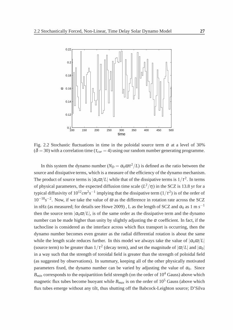
2.2 Stochastically Forced, Non-Linear, Time Delay Solar Dynamo Model 27
100 150 200 250 300 350 400 450 5000.1
0.12
0.14
0.16
0.18
0.2
0.22
time
α
Fig. 2.2 Stochastic fluctuations in time in the poloidal source termα at a level of 30%(δ = 30) with a correlation time (τcor = 4) using our random number generating programme.
In this system the dynamo number (ND = α0ωτ2/L) is defined as the ratio between the
source and dissipative terms, which is a measure of the efficiency of the dynamo mechanism.
The product of source terms is|α0ω/L| while that of the dissipative terms is 1/τ2. In terms
of physical parameters, the expected diffusion time scale (L2/η) in the SCZ is 13.8 yr for a
typical diffusivity of 1012cm2s−1 implying that the dissipative term (1/τ2) is of the order of
10−18s−2. Now, if we take the value ofω as the difference in rotation rate across the SCZ
in nHz (as measured; for details see Howe 2009) , L as the length of SCZ andα0 as 1 ms−1
then the source term|α0ω/L|, is of the same order as the dissipative term and the dynamo
number can be made higher than unity by slightly adjusting the α coefficient. In fact, if the
tachocline is considered as the interface across which flux transport is occurring, then the
dynamo number becomes even greater as the radial differential rotation is about the same
while the length scale reduces further. In this model we always take the value of|α0ω/L|(source term) to be greater than 1/τ2 (decay term), and set the magnitude of|ω/L| and|α0|in a way such that the strength of toroidal field is greater than the strength of poloidal field
(as suggested by observations). In summary, keeping all of the other physically motivated
parameters fixed, the dynamo number can be varied by adjusting the value ofα0. Since
Bmin corresponds to the equipartition field strength (on the order of 104 Gauss) above which
magnetic flux tubes become buoyant whileBmax is on the order of 105 Gauss (above which
flux tubes emerge without any tilt, thus shutting off the Babcock-Leighton source; D’Silva
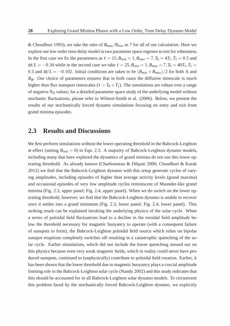
28 Exploring Grand Minima Phases with a Low Order, Time Delay Dynamo Model
& Choudhuri 1993), we take the ratio ofBmax/Bmin as 7 for all of our calculation. Here we
explore our low order time delay model in two parameter spaceregimes to test for robustness.
In the first case we fix the parameters asτ = 15,Bmin= 1,Bmax= 7,T0 = 4T1,T1 = 0.5 and
ω/L =−0.34 while in the second case we takeτ = 25,Bmin= 1,Bmax= 7,T0 = 40T1,T1 =
0.5 andω/L = −0.102. Initial conditions are taken to be(Bmin+Bmax)/2 for both A and
Bφ . Our choice of parameters ensures that in both cases the diffusive timescale is much
higher than flux transport timescales (τ > T0+T1). The simulations are robust over a range
of negativeND values; for a detailed parameter space study of the underlying model without
stochastic fluctuations, please refer to Wilmot-Smith et al. (2006). Below, we present the
results of our stochastically forced dynamo simulations focusing on entry and exit from
grand minima episodes.
2.3 Results and Discussions
We first perform simulations without the lower operating threshold in the Babcock-Leighton
α-effect (settingBmin = 0) in Eqn. 2.3. A majority of Babcock-Leighton dynamo models,
including many that have explored the dynamics of grand minima do not use this lower op-
erating threshold. As already known (Charbonneau & Dikpati2000; Choudhuri & Karak
2012) we find that the Babcock-Leighton dynamo with this setup generate cycles of vary-
ing amplitudes, including episodes of higher than average activity levels (grand maxima)
and occasional episodes of very low amplitude cycles reminiscent of Maunder-like grand
minima (Fig. 2.3, upper panel; Fig. 2.4, upper panel). When we do switch on the lower op-
erating threshold, however, we find that the Babcock-Leighton dynamo is unable to recover
once it settles into a grand minimum (Fig. 2.3, lower panel; Fig. 2.4, lower panel). This
striking result can be explained invoking the underlying physics of the solar cycle. When
a series of poloidal field fluctuations lead to a decline in thetoroidal field amplitude be-
low the threshold necessary for magnetic buoyancy to operate (with a consequent failure
of sunspots to form), the Babcock-Leighton poloidal field source which relies on bipolar
sunspot eruptions completely switches off resulting in a catastrophic quenching of the so-
lar cycle. Earlier simulations, which did not include the lower quenching missed out on
this physics because even very weak magnetic fields, which inreality could never have pro-
duced sunspots, continued to (unphysically) contribute topoloidal field creation. Earlier, it
has been shown that the lower threshold due to magnetic buoyancy plays a crucial amplitude
limiting role in the Babcock-Leighton solar cycle (Nandy 2002) and this study indicates that
this should be accounted for in all Babcock-Leighton solar dynamo models. To circumvent
this problem faced by the stochastically forced Babcock-Leighton dynamo, we explicitly
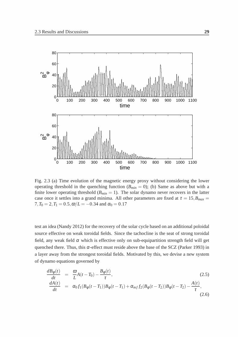
2.3 Results and Discussions 29
0 100 200 300 400 500 600 700 800 900 1000 11000
20
40
60
80
time
Bφ2
0 100 200 300 400 500 600 700 800 900 1000 11000
20
40
60
80
time
Bφ2
Fig. 2.3 (a) Time evolution of the magnetic energy proxy without considering the loweroperating threshold in the quenching function (Bmin = 0); (b) Same as above but with afinite lower operating threshold (Bmin = 1). The solar dynamo never recovers in the lattercase once it settles into a grand minima. All other parameters are fixed atτ = 15,Bmax=7,T0 = 2,T1 = 0.5,ω/L =−0.34 andα0 = 0.17
test an idea (Nandy 2012) for the recovery of the solar cycle based on an additional poloidal
source effective on weak toroidal fields. Since the tachocline is the seat of strong toroidal
field, any weak fieldα which is effective only on sub-equipartition strength fieldwill get
quenched there. Thus, thisα-effect must reside above the base of the SCZ (Parker 1993) in
a layer away from the strongest toroidal fields. Motivated bythis, we devise a new system
of dynamo equations governed by
dBφ (t)
dt=
ωL
A(t−T0)−Bφ (t)
τ, (2.5)
dA(t)dt
= α0 f1(Bφ (t −T1))Bφ (t −T1)+αm f f2(Bφ (t −T2))Bφ(t −T2)−A(t)
τ,
(2.6)
30 Exploring Grand Minima Phases with a Low Order, Time Delay Dynamo Model
0 200 400 600 800 1000 1200 1400 1600 1800 2000 22000
20
40
60
80
time
Bφ2
0 200 400 600 800 1000 1200 1400 1600 1800 2000 22000
20
40
60
80
time
Bφ2
Fig. 2.4 (a) Time evolution of the magnetic energy proxy without considering the loweroperating threshold in the quenching function (Bmin = 0); (b) Same as above but with afinite lower operating threshold (Bmin = 1). The solar dynamo never recovers in the lattercase once it settles into a grand minima. All other parameters are fixed atτ = 25,Bmax=7,T0 = 20,T1 = 0.5,ω/L =−0.102 andα0 = 0.051
where f2, the quenching function for the weak field poloidal sourceαm f is shown in Fig. 2.1
and is parameterized by
f2 =erfc(B2
φ (t−T2)−B2eq)
2. (2.7)
TakingBeq= 1 ensures that the weak field source term gets quenched at or below the lower
operating threshold for the Babcock-Leightonα and the former, therefore, can be inter-
preted to be the mean fieldα effect. In equation 2.6, the time delayT2 is the time necessary
for the toroidal field to enter the source region where the additional, weak-fieldα effect is
located.
If T2 = 0, i.e. the generation layer of the additionalα effect is coincident with theΩeffect (layer) then we find that the stochastically forced dynamo again fails to recover from
a grand minimum. This is reminiscent of the original motivation behind the introduction of
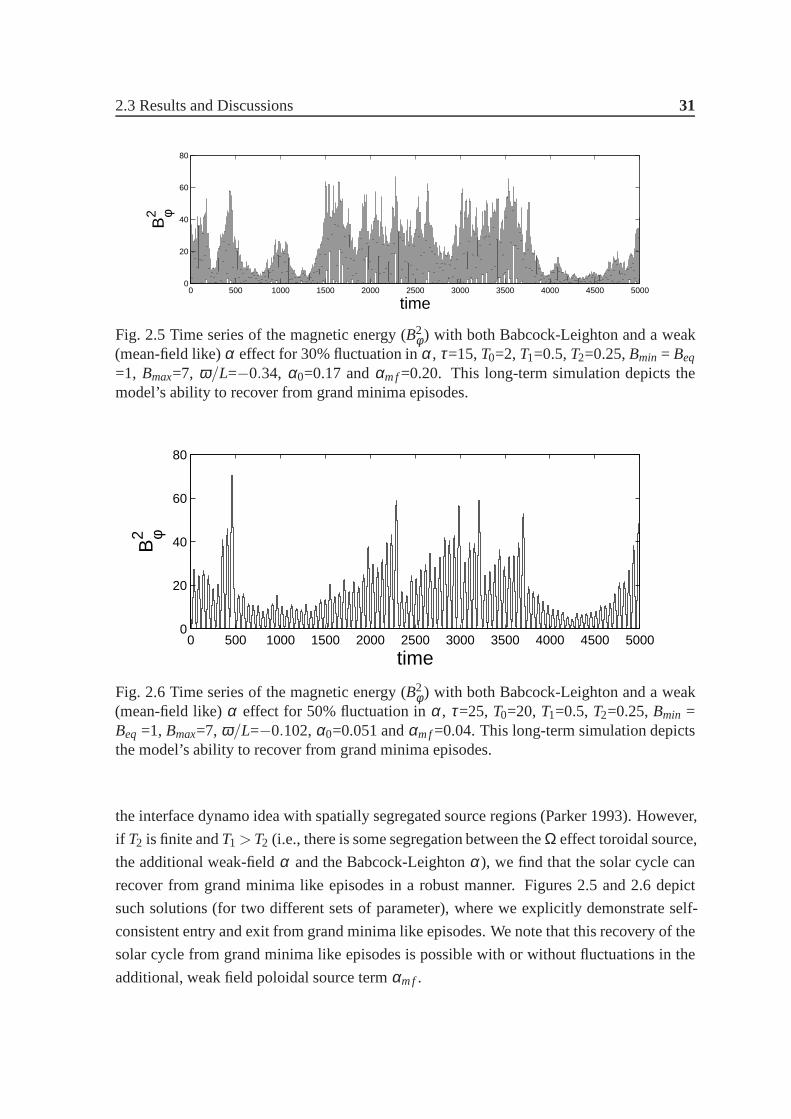
2.3 Results and Discussions 31
0 500 1000 1500 2000 2500 3000 3500 4000 4500 50000
20
40
60
80
time
Bφ2
Fig. 2.5 Time series of the magnetic energy (B2φ ) with both Babcock-Leighton and a weak
(mean-field like)α effect for 30% fluctuation inα, τ=15,T0=2,T1=0.5,T2=0.25,Bmin = Beq
=1, Bmax=7, ω/L=−0.34, α0=0.17 andαm f=0.20. This long-term simulation depicts themodel’s ability to recover from grand minima episodes.
0 500 1000 1500 2000 2500 3000 3500 4000 4500 50000
20
40
60
80
time
Bφ2
Fig. 2.6 Time series of the magnetic energy (B2φ ) with both Babcock-Leighton and a weak
(mean-field like)α effect for 50% fluctuation inα, τ=25, T0=20, T1=0.5,T2=0.25,Bmin =Beq =1, Bmax=7, ω/L=−0.102,α0=0.051 andαm f=0.04. This long-term simulation depictsthe model’s ability to recover from grand minima episodes.
the interface dynamo idea with spatially segregated sourceregions (Parker 1993). However,
if T2 is finite andT1 >T2 (i.e., there is some segregation between theΩ effect toroidal source,
the additional weak-fieldα and the Babcock-Leightonα), we find that the solar cycle can
recover from grand minima like episodes in a robust manner. Figures 2.5 and 2.6 depict
such solutions (for two different sets of parameter), wherewe explicitly demonstrate self-
consistent entry and exit from grand minima like episodes. We note that this recovery of the
solar cycle from grand minima like episodes is possible withor without fluctuations in the
additional, weak field poloidal source termαm f.
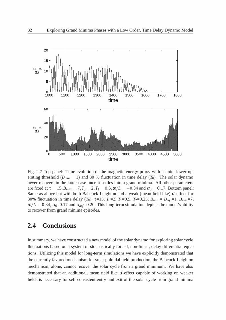
32 Exploring Grand Minima Phases with a Low Order, Time Delay Dynamo Model
1000 1100 1200 1300 1400 1500 1600 1700 18000
5
10
15
20
time
B2 φ
0 500 1000 1500 2000 2500 3000 3500 4000 4500 50000
20
40
60
time
B2 φ
Fig. 2.7 Top panel: Time evolution of the magnetic energy proxy with a finite lower op-erating threshold (Bmin = 1) and 30 % fluctuation in time delay (T0). The solar dynamonever recovers in the latter case once it settles into a grandminima. All other parametersare fixed atτ = 15,Bmax= 7,T0 = 2,T1 = 0.5,ω/L =−0.34 andα0 = 0.17. Bottom panel:Same as above but with both Babcock-Leighton and a weak (mean-field like) α effect for30% fluctuation in time delay (T0), τ=15, T0=2, T1=0.5, T2=0.25,Bmin = Beq =1, Bmax=7,ω/L=−0.34,α0=0.17 andαm f=0.20. This long-term simulation depicts the model’s abilityto recover from grand minima episodes.
2.4 Conclusions
In summary, we have constructed a new model of the solar dynamo for exploring solar cycle
fluctuations based on a system of stochastically forced, non-linear, delay differential equa-
tions. Utilizing this model for long-term simulations we have explicitly demonstrated that
the currently favored mechanism for solar poloidal field production, the Babcock-Leighton
mechanism, alone, cannot recover the solar cycle from a grand minimum. We have also
demonstrated that an additional, mean field likeα-effect capable of working on weaker
fields is necessary for self-consistent entry and exit of thesolar cycle from grand minima

2.4 Conclusions 33
episodes. We have demonstrated that our results and conclusions hold over two very di-
verse regimes of parameter choices. Although we have utilized fluctuations in the poloidal
source in our study, we do not claim that this is the only possible source of fluctuations in
the solar cycle. We also point out that our model results are robust if we run simulations
considering fluctuations in time delay (Fig. 2.7). We note that simulations motivated from
this current study and based on a spatially extended dynamo model in a solar-like geometry
supports the results from this mathematical time delay model (Passos et al. 2014). Taken
together, these strengthen the conclusion that a mean field like α-effect effective on weak
toroidal fields must be functional in the Sun’s convection zone and that this is vitally impor-
tant for the solar cycle, even if the dominant contribution to the poloidal field comes from
the Babcock-Leighton mechanism during normal activity phases.

Chapter 3
Strong Hemispheric Asymmetry can
Trigger Parity Changes in the Sunspot
Cycle
Although sunspots have been systematically observed on theSun’s surface over the last
four centuries, their magnetic properties have been revealed and documented only since the
early 1900s. Sunspots typically appear in pairs of oppositemagnetic polarity which have a
systematic orientation. This polarity orientation is opposite across the equator – a trend that
has persisted over the last century since observations of sunspot magnetic fields exist. Taken
together with the configuration of the global poloidal field of the Sun – that governs the
heliospheric open flux and cosmic ray flux at Earth – this phenomena is consistent with the
dipolar parity state of an underlying magnetohydrodynamicdynamo mechanism. Although,
hemispheric asymmetry in the emergence of sunspots is observed in the Sun, a parity shift
has never been observed. We simulate hemispheric asymmetrythrough introduction of
random fluctuations in a computational dynamo model of the solar cycle and demonstrate
that changes in parity are indeed possible over long time-scales. In particular, we find that
a parity shift in the underlying nature of the sunspot cycle is more likely to occur when
sunspot activity dominates in any one hemisphere for a time which is significantly longer
compared to the sunspot cycle period. Our simulations suggest that the sunspot cycle may
have resided in quadrupolar parity states in the distant past, and provides a possible pathway
for predicting parity flips in the future.
36 Strong Hemispheric Asymmetry can Trigger Parity Changes inthe Sunspot Cycle
3.1 Introduction
Samuel Heinrich Schwabe discovered the 11 year solar cycle in 1843, but detailed observa-
tions about the dipolar nature of solar magnetic fields existonly for last hundred years (Hale
et al. 1919). One may pose the question whether solar magnetic fields have always been in
the dipolar state?
To investigate this issue we use an axisymmetric kinematic flux transport solar dynamo
model which involves the generation and recycling of the toroidal and poloidal field (Parker
1955). In this model, the toroidal field is produced by stretching of poloidal field lines
at the base of the convection zone due to strong differentialrotation (Parker 1955) and the
poloidal field is generated through a combination of mean field α-effect due to helical turbu-
lence in the solar convection zone (Parker 1955) and the Babcock-Leighton mechanism due
to decay and dispersal of tilted bipolar sunspot region at the near-surface layers (Babcock
1961; Leighton 1969). The kinematic flux transport dynamo model based on the Babcock-
Leighton mechanism for poloidal field generation has been successful in explaining different
observational aspects of the solar cycle (Dikpati & Charbonneau 1999; Nandy & Choudhuri
2002; Chatterjee et al. 2004; Goel & Choudhuri 2009; Nandy etal. 2011; Karak & Nandy
2012; DeRosa et al. 2012). Recent observations also lend strong support to the Babcock-
Leighton mechanism as a primary source for poloidal field generation (Dasi-Espuig et al.
2010; Muñoz-Jaramillo et al. 2013).
It is widely thought that stochastic fluctuations in the poloidal field generation mecha-
nism is the primary source for irregularity in the solar cycle (Hoyng 1988; Choudhuri 1992;
Charbonneau & Dikpati 2000; Charbonneau et al. 2004). In theBabcock-Leighton frame-
work, poloidal field generation depends on the tilt angle of bipolar sunspot pairs, which is
imparted by the action of Coriolis force on buoyantly risingtoroidal flux tubes from the
base of the solar convection zone. Observational scatter oftilt angles around the mean
given by Joy’s law may be produced by turbulent buffeting that a rising flux tube encounters
during its journey through the convection zone (Longcope & Choudhuri 2002). Thus the
Babcock-Leighton mechanism for poloidal field generation is not a deterministic process
but a random one (Choudhuri et al. 2007). Another major source in solar cycle irregularity
is fluctuations in the meridional circulation (Lopes & Passos 2009; Karak 2010).
On the one hand, two different types of symmetries are obtained, in general, in solutions
of the dynamo equations. The global magnetic field is of dipolar nature (dipolar or odd par-
ity) if the toroidal field is antisymmetric across the equator; conversely, if the toroidal field
3.1 Introduction 37
is symmetric across the equator then the global field is of quadrupolar nature (quadrupolar
or even parity). Some previous studies have found solutionsthat are of quadrupolar nature
using low diffusivity in their kinematic dynamo models. It has been suggested that an addi-
tional alpha effect at the base of the convection zone is necessary to produce the observed
dipolar parity (Dikpati & Gilman 2001; Bonanno et al. 2002).However, other studies sug-
gest that strong hemispheric coupling by higher diffusivity is necessary for generation of
the global dipolar magnetic field without the presence of an additional alpha effect at the
base of the convection zone (Chatterjee et al. 2004; Chatterjee & Choudhuri 2006; Hotta &
Yokoyama 2010). These past studies have been inspired with the primary aim of ensuring
dipolar solutions to the dynamo equations with the notion that the solar dynamo has always
persisted in the dipolar parity state with antisymmetric toroidal fields across the equator.
On the other hand, unequal solar activity in northern and southern hemispheres (known
as hemispheric asymmetry) is well documented (Waldmeier 1955, 1971; Chowdhury et al.
2013; McClintock & Norton 2013). Observational evidence ofstrong hemispheric asym-
metry exists during the onset of grand-minima like episodes(Sokoloff & Nesme-Reibes
1994). Theoretical and observational studies also suggestthat hemispheric polar field at the
minimum of the solar cycle can be used as a precursor to predict the amplitude of the next
cycle (Schaten et al. 1978; Schaten 2005; Jiang et al. 2007; Karak & Nandy 2012; Muñoz-
Jaramillo et al. 2013). Thus possibly, the hemispheric asymmetry of the polar field at solar
minima may be responsible for the hemispheric asymmetry in the next cycle too. Feeding
the data of the polar flux of previous cycles in kinematic solar dynamo models, some studies
are able to explain hemispheric asymmetry like phenomenon in the current cycle (Goel &
Choudhuri, 2009). Details about hemispheric coupling and hemispheric asymmetry can be
found in a review paper by Norton et al. (2014).
To explore hemispheric asymmetry and parity issues and their inter-relationship, we in-
troduce stochastic fluctuations in the Babcock-Leighton poloidal field source and find that
stochastic fluctuations can trigger the solar cycle into grand minima like episodes. As pro-
posed earlier, we confirm that an additionalα-effect is necessary for cycle recovery. In
the next step, we introduce stochastic fluctuations in both the Babcock-Leighton mecha-
nism and the additional mean fieldα-effect and find dynamo solutions can self-consistently
change parity. The above result begs the question whether itis possible to predict parity flips
in the Sun. We find that parity flips in the sunspot cycle tend tooccur when solar activity
in one hemisphere strongly dominates over the other hemisphere for a period of time signif-
icantly longer than the sunspot cycle timescale. However, strong domination of activity in
one hemisphere does not necessarily always guarantee a parity change.
38 Strong Hemispheric Asymmetry can Trigger Parity Changes inthe Sunspot Cycle
3.2 Model
Our model is based onαΩ dynamo equations in the axisymmetric spherical formulation
wherein the dynamo equations are:
∂A∂ t
+1s[vp ·∇(sA)] = η
(∇2− 1
s2
)A+S(r,θ ,B), (3.1)
∂B∂ t
+s
[vp ·∇
(Bs
)]+(∇ ·vp)B= η
(∇2− 1
s2
)B+s
([∇× (Aeφ )
]·∇Ω
)+
1s
∂ (sB)∂ r
∂η∂ r
,
(3.2)
where,B(r,θ) (i.e. Bφ ) andA(r,θ) are the toroidal and vector potential for the poloidal
components of the magnetic field respectively. HereΩ is the differential rotation,vp is the
meridional flow,η is the turbulent magnetic diffusivity ands= r sin(θ).Here, we use a two step radially dependent magnetic diffusivity profile as described in
Muñoz-Jaramilloet al. (2009). In our case, the diffusivity at the bottom of convection zone
is 108cm2/s, diffusivity in the convection zone is 1011cm2/s and supergranular diffusivity
is 5×1012cm2/s. rcz= 0.73R⊙, dcz= 0.025R⊙, rsg= 0.95R⊙ anddsg= 0.015R⊙ describes
the transition from one diffusivity value to another. We also use the same differential ro-
tation profile as described inMuñoz-Jaramilloet al. (2009). We generate the meridional
circulation profile (vp) for a compressible flow inside the convection zone by using astream
function along with mass conservation constraint:
vp (r,θ) =1
ρ(r)∇×
(ψ(r,θ)eφ
). (3.3)
which is estimated from the stream function (defined within 0≤ θ ≤ π/2, i.e., in the north-
ern hemisphere) as described in Chatterjee, Nandy and Choudhuri (2004):
ψr sinθ = ψ0(r −Rp)sin
[π(r −Rp)
(R⊙−Rp)
]1−e−β1θ ε1−eβ2(θ−π/2)e−((r−r0)/Γ)2,(3.4)
whereψ0 is the factor which determines the maximum speed of the flow. We use the fol-
lowing parameter valuesβ1 = 1.5,β2 = 1.8,ε = 2.0000001, r0 = (R⊙−Rb)/4,Γ = 3.47×10⁸ m,γ = 0.95,m= 3/2. HereRp = 0.64R⊙ is the penetration depth of the meridional
flow. The meridional circulation profile in the southern hemisphere is generated by a mirror
reflection of the velocity profile across the equator. In thiswork, we use the surface value
of meridional circulation as 17ms−1.
3.2 Model 39
Recent observations and theory both indicate that the Babcock-Leighton mechanism
for poloidal field creation plays an important role in the solar cycle. In Equation (3.1),
S(r,θ ,B) represents the Babcock-Leighton mechanism. But modellingthis mechanism to
capture correctly the underlying physics is a challenging task. Two different approaches
exist in the kinematic dynamo literature to model Babcock-Leighton mechanism-one is
alpha-coefficient formulation and another is double ring approach proposed by Durney
(1995). Nandy & Choudhuri (2001) has shown that these two different approaches for mod-
elling Babcock-Leighton mechanism produce qualitativelysimilar result. However Muñoz-
Jaramillo et al. (2010) has shown that double ring approach is more successful in capturing
the observed surface dynamics compared to the alpha-coefficient formulation. Motivated by
this, here we model the Babcock-Leighton mechanism (i.e., poloidal field source term) by
the emergence and flux dispersal of double-rings structures.
3.2.1 Modelling Active Regions as Double Rings and Recreating the
poloidal field
We model the Babcock-Leighton mechanism by the methods of double ring proposed by
Durney (1997) and subsequently used by some other groups (Nandy & Choudhuri 2001;
Muñoz-Jaramillo et al. 2010; Nandy et al. 2011). In this algorithm we define theφ compo-
nent of potential vectorA corresponding to active region as:
Aar(r,θ , t) = K1A(Φ, t)F(r)G(θ), (3.5)
whereK1 is a constant which ensures super-critical solutions and strength of ring doublet is
defined byA(Φ, t). Φ is basically the magnetic flux. We defineF(r) as:
F(r) =
0 r < R⊙−Rar
1r sin2
[π
2Rar(r − (R⊙−Rar))
]r ≥ R⊙−Rar
, (3.6)
whereR⊙ is the solar radius andRar = 0.15R⊙. R⊙−Rar is the radial extent of the active
regions, i.e., how deep they extend from the surface. This extent (surface to 0.85R⊙) is
motivated from results indicating that active region flux tube disconnection happens around
this depth in the convection zone (Longcope & Choudhuri 2002). We defineG(θ) in integral
form as:
G(θ) =1
sinθ
∫ θ
0[B−(θ ′)+B+(θ ′)]sin(θ ′)dθ ′, (3.7)
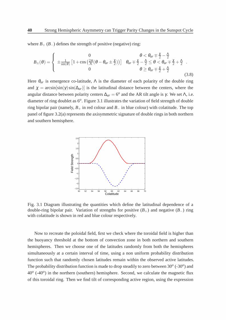
40 Strong Hemispheric Asymmetry can Trigger Parity Changes inthe Sunspot Cycle
whereB+ (B−) defines the strength of positive (negative) ring:
B±(θ) =
0 θ < θar ∓ χ2 − Λ
2
± 1sin(θ )
[1+cos
(2πΛ (θ −θar ± χ
2))]
θar ∓ χ2 − Λ
2 ≤ θ < θar ∓ χ2 +
Λ2
0 θ ≥ θar ∓ χ2 +
Λ2
.
(3.8)
Here θar is emergence co-latitude,Λ is the diameter of each polarity of the double ring
and χ = arcsin[sin(γ)sin(∆ar)] is the latitudinal distance between the centers, where the
angular distance between polarity centers∆ar = 6o and the AR tilt angle isγ. We setΛ, i.e.
diameter of ring doublet as 6o. Figure 3.1 illustrates the variation of field strength of double
ring bipolar pair (namely,B+ in red colour andB− in blue colour) with colatitude. The top
panel of figure 3.2(a) represents the axisymmetric signature of double rings in both northern
and southern hemisphere.
50 52 54 56 58 60 62 64 66 68 70−2.5
−2
−1.5
−1
−0.5
0
0.5
1
1.5
2
2.5
Colatitude
Fie
ld S
tren
gth
Fig. 3.1 Diagram illustrating the quantities which define the latitudinal dependence of adouble-ring bipolar pair. Variation of strengths for positive (B+) and negative (B−) ringwith colatitude is shown in red and blue colour respectively.
Now to recreate the poloidal field, first we check where the toroidal field is higher than
the buoyancy threshold at the bottom of convection zone in both northern and southern
hemispheres. Then we choose one of the latitudes randomly from both the hemispheres
simultaneously at a certain interval of time, using a non uniform probability distribution
function such that randomly chosen latitudes remain withinthe observed active latitudes.
The probability distribution function is made to drop steadily to zero between 30o (-30o) and
40o (-40o) in the northern (southern) hemisphere. Second, we calculate the magnetic flux
of this toroidal ring. Then we find tilt of corresponding active region, using the expression
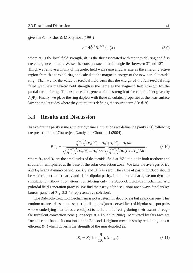
3.3 Results and Discussion 41
given in Fan, Fisher & McClymont (1994)
γ ∝ Φ1/40 B−5/4
0 sin(λ ), (3.9)
whereB0 is the local field strength,Φ0 is the flux associated with the toroidal ring andλ is
the emergence latitude. We set the constant such that tilt angle lies between 3o and 12o.
Third, we remove a chunk of magnetic field with same angular size as the emerging active
region from this toroidal ring and calculate the magnetic energy of the new partial toroidal
ring. Then we fix the value of toroidal field such that the energy of the full toroidal ring
filled with new magnetic field strength is the same as the magnetic field strength for the
partial toroidal ring. This exercise also generated the strength of the ring doublet given by
A(Φ). Finally, we place the ring duplets with these calculated properties at the near-surface
layer at the latitudes where they erupt, thus defining the source termS(r,θ ,B).
3.3 Results and Discussion
To explore the parity issue with our dynamo simulations we define the parityP(t) following
the prescription of Chatterjee, Nandy and Choudhuri (2004):
P(t) =
∫ t+T/2t−T/2 (BN(t ′)−BN)(BS(t ′)−BS)dt′
√∫ t+T/2t−T/2 (BN(t ′)−BN)2dt′
√∫ t+T/2t−T/2 (BS(t ′)−BS)2dt′
, (3.10)
whereBN andBS are the amplitudes of the toroidal field at 25 latitude in both northern and
southern hemispheres at the base of the solar convection zone. We take the averages ofBN
andBS over a dynamo period (i.e.BN andBS ) as zero. The value of parity function should
be +1 for quadrupolar parity and -1 for dipolar parity. In thefirst scenario, we run dynamo
simulations without fluctuations, considering only the Babcock-Leighton mechanism as a
poloidal field generation process. We find the parity of the solutions are always dipolar (see
bottom panels of Fig. 3.2 for representative solution).
The Babcock-Leighton mechanism is not a deterministic process but a random one. This
random nature arises due to scatter in tilt angles (an observed fact) of bipolar sunspot pairs
whose underlying flux tubes are subject to turbulent buffeting during their ascent through
the turbulent convection zone (Longcope & Choudhuri 2002).Motivated by this fact, we
introduce stochastic fluctuations in the Babcock-Leightonmechanism by redefining the co-
efficientK1 (which governs the strength of the ring doublet) as:
K1 = K0[1+δ
100σ(t,τcor)], (3.11)
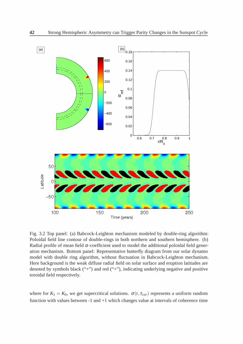
42 Strong Hemispheric Asymmetry can Trigger Parity Changes inthe Sunspot Cycle
−600
−400
−200
0
200
400
600
0.6 0.7 0.8 0.9 10
0.02
0.04
0.06
0.08
0.1
0.12
0.14
0.16
0.18
r/R0
α mf
(a) (b)
Fig. 3.2 Top panel: (a) Babcock-Leighton mechanism modeledby double-ring algorithm:Poloidal field line contour of double-rings in both northernand southern hemisphere. (b)Radial profile of mean fieldα-coefficient used to model the additional poloidal field gener-ation mechanism. Bottom panel: Representative butterfly diagram from our solar dynamomodel with double ring algorithm, without fluctuation in Babcock-Leighton mechanism.Here background is the weak diffuse radial field on solar surface and eruption latitudes aredenoted by symbols black (“+”) and red (“+”), indicating underlying negative and positivetoroidal field respectively.
where forK1 = K0, we get supercritical solutions.σ(t,τcor) represents a uniform random
function with values between -1 and +1 which changes value atintervals of coherence time
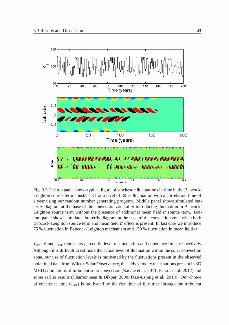
3.3 Results and Discussion 43
Fig. 3.3 The top panel shows typical figure of stochastic fluctuations in time in the Babcock-Leighton source term constant K1 at a level of 30 % fluctuationwith a correlation time of1 year using our random number generating program. Middle panel shows simulated but-terfly diagram at the base of the convection zone after introducing fluctuation in Babcock-Leighton source term without the presence of additional mean field α source term. Bot-tom panel shows simulated butterfly diagram at the base of theconvection zone when bothBabcock-Leighton source term and mean fieldα effect is present. In last case we introduce75 % fluctuation in Babcock-Leighton mechanism and 150 % fluctuation in mean fieldα.
τcor. δ andτcor represents percentile level of fluctuation and coherence time, respectively.
Although it is difficult to estimate the actual level of fluctuation within the solar convection
zone, our use of fluctuation levels is motivated by the fluctuations present in the observed
polar field data from Wilcox Solar Observatory, the eddy velocity distributions present in 3D
MHD simulations of turbulent solar convection (Racine et al. 2011; Passos et al. 2012) and
some earlier results (Charbonneau & Dikpati 2000; Dasi-Espuig et al. 2010). Our choice
of coherence time (τcor) is motivated by the rise time of flux tube through the turbulent
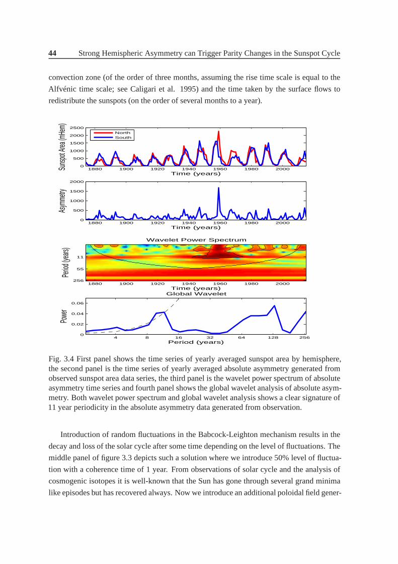
44 Strong Hemispheric Asymmetry can Trigger Parity Changes inthe Sunspot Cycle
convection zone (of the order of three months, assuming the rise time scale is equal to the
Alfvénic time scale; see Caligari et al. 1995) and the time taken by the surface flows to
redistribute the sunspots (on the order of several months toa year).
1880 1900 1920 1940 1960 1980 20000
500
1000
1500
2000
2500
Time (years)
Sunsp
ot Are
a (mH
em)
NorthSouth
1880 1900 1920 1940 1960 1980 20000
500
1000
1500
2000
Time (years)
Asym
metry
Time (years)
Perio
d (yea
rs)
Wavelet Power Spectrum
1880 1900 1920 1940 1960 1980 2000
11
55
256
4 8 16 32 64 128 2560
0.02
0.04
0.06
Powe
r
Period (years)
Global Wavelet
Fig. 3.4 First panel shows the time series of yearly averagedsunspot area by hemisphere,the second panel is the time series of yearly averaged absolute asymmetry generated fromobserved sunspot area data series, the third panel is the wavelet power spectrum of absoluteasymmetry time series and fourth panel shows the global wavelet analysis of absolute asym-metry. Both wavelet power spectrum and global wavelet analysis shows a clear signature of11 year periodicity in the absolute asymmetry data generated from observation.
Introduction of random fluctuations in the Babcock-Leighton mechanism results in the
decay and loss of the solar cycle after some time depending onthe level of fluctuations. The
middle panel of figure 3.3 depicts such a solution where we introduce 50% level of fluctua-
tion with a coherence time of 1 year. From observations of solar cycle and the analysis of
cosmogenic isotopes it is well-known that the Sun has gone through several grand minima
like episodes but has recovered always. Now we introduce an additional poloidal field gener-
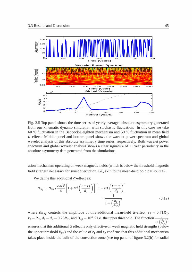
3.3 Results and Discussion 45
500 550 600 650 700 750 8000
50
100
150
200
Time (years)
Asym
metry
Time (year)
Perio
d (yea
rs)
Wavelet Power Spectrum
500 1000 1500 2000 2500 3000 3500 4000
11
55
256
4 8 16 32 64 128 2560
1
2
3
4
5
x 104
Powe
r
Period (years)
Global Wavelet
Fig. 3.5 Top panel shows the time series of yearly averaged absolute asymmetry generatedfrom our kinematic dynamo simulation with stochastic fluctuation. In this case we take60 % fluctuation in the Babcock-Leighton mechanism and 50 % fluctuation in mean fieldα-effect. Middle panel and bottom panel shows the wavelet power spectrum and globalwavelet analysis of this absolute asymmetry time series, respectively. Both wavelet powerspectrum and global wavelet analysis shows a clear signature of 11 year periodicity in theabsolute asymmetry data generated from the simulations.
ation mechanism operating on weak magnetic fields (which is below the threshold magnetic
field strength necessary for sunspot eruption, i.e., akin tothe mean-field poloidal source).
We define this additionalα-effect as:
αm f = α0m fcosθ
4
[1+erf
(r − r1
d1
)][1−erf
(r − r2
d2
)]
× 1
1+(
BφBup
)2 (3.12)
whereα0m f controls the amplitude of this additional mean-fieldα-effect, r1 = 0.71R⊙,
r2=R⊙, d1=d2=0.25R⊙, andBup= 104 G i.e. the upper threshold. The function 1
1+( Bφ
Bup
)2
ensures that this additionalα effect is only effective on weak magnetic field strengths (below
the upper thresholdBup) and the value ofr1 andr2 confirms that this additional mechanism
takes place inside the bulk of the convection zone (see top panel of figure 3.2(b) for radial
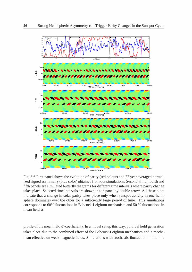
46 Strong Hemispheric Asymmetry can Trigger Parity Changes inthe Sunspot Cycle
0 500 1000 1500 2000 2500 3000 3500 4000−1
−0.8
−0.6
−0.4
−0.2
0
0.2
0.4
0.6
0.8
1
Time (years)
Signed Asymmetry
Parity
Fig. 3.6 First panel shows the evolution of parity (red colour) and 22 year averaged normal-ized signed asymmetry (blue color) obtained from our simulations. Second, third, fourth andfifth panels are simulated butterfly diagrams for different time intervals where parity changetakes place. Selected time intervals are shown in top panel by double arrow. All these plotsindicate that a change in solar parity takes place only when sunspot activity in one hemi-sphere dominates over the other for a sufficiently large period of time. This simulationscorresponds to 60% fluctuations in Babcock-Leighton mechanism and 50 % fluctuations inmean fieldα.
profile of the mean fieldα-coefficient). In a model set up this way, poloidal field generation
takes place due to the combined effect of the Babcock-Leighton mechanism and a mecha-
nism effective on weak magnetic fields. Simulations with stochastic fluctuation in both the
3.3 Results and Discussion 47
Babcock-Leighton mechanism and an additional mean fieldα-effect show that the cycle re-
covers from grand minima-like episodes and regains normal activity levels (see bottom panel
of figure 3.3 for representative solution with fluctuations in both the Babcock-Leighton and
mean fieldα). This result confirms our earlier results based on somewhatdifferent dynamo
models (Hazra et al. 2014; Passos et al. 2014).
Introducing fluctuations in both the Babcock-Leighton source (Kar) and mean field poloidal
source terms (αm f), we find the parity of dynamo solutions change (see top panels of figure
3.6 and 3.7). Earlier studies indicate that the dipolar parity of dynamo solutions is associated
with strong hemispheric coupling – which can be obtained either by increasing diffusivity or
by introducing an additional mean fieldα effect (distributed through the convection zone, or
tachocline) (Dikpati & Gilman 2001; Chatterjee et al. 2004). These models do not consider
stochastic fluctuation in their simulation. Introducing stochastic fluctuations in dynamo
simulations we always find solutions of single periodicity in both hemispheres even if we
introduce very large fluctuations in poloidal field source terms (both BL and mean fieldαeffect).
What is the cause of parity change in our model? One possible reason is the different
levels of fluctuations in poloidal field source terms associated with northern and southern
hemispheres. Stochastic fluctuations or randomness in the poloidal source is plausibly at
the heart of hemispheric asymmetry (Hoyng 1988). Thus we think that there may be a rela-
tionship between hemispheric asymmetry and parity change.To investigate the relationship
between parity and hemispheric asymmetry, we have to define hemispheric asymmetry in
the context of our simulations. In our kinematic flux transport dynamo model, we model the
Babcock-Leighton mechanism by double ring algorithm. We believe that double ring algo-
rithm is a more realistic way to capture the essence of the Babcock-Leighton mechanism as
well as sunspots. For this work, we take the difference between double ring eruptions in the
northern and southern hemispheres as a measure of hemispheric asymmetry. We call this
difference the signed asymmetry and only the magnitude of this difference as asymmetry
for the rest of the chapter.
We find no north-south asymmetry in the simulated solar cycleif we perform dynamo
simulations without stochastic fluctuation. Thus our result confirms the idea that stochastic
fluctuation is the cause for hemispheric asymmetry. Interestingly, we find that yearly aver-
aged absolute asymmetry obtained from our simulation is notstochastic, rather it shows a
systematic periodic behaviour. We also find that hemispheric asymmetry obtained from our
simulation is stronger at solar cycle maximum but also sometimes significant at solar cycle
minima. We note that maximum amplitude of yearly averaged absolute asymmetry time
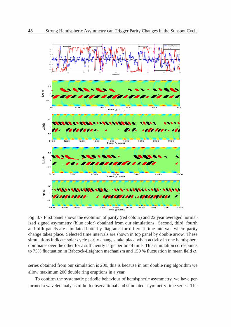
48 Strong Hemispheric Asymmetry can Trigger Parity Changes inthe Sunspot Cycle
0 500 1000 1500 2000 2500 3000 3500 4000−1
−0.8
−0.6
−0.4
−0.2
0
0.2
0.4
0.6
0.8
1
Time (years)
Signed Asymmetry
Parity
Fig. 3.7 First panel shows the evolution of parity (red colour) and 22 year averaged normal-ized signed asymmetry (blue color) obtained from our simulations. Second, third, fourthand fifth panels are simulated butterfly diagrams for different time intervals where paritychange takes place. Selected time intervals are shown in toppanel by double arrow. Thesesimulations indicate solar cycle parity changes take placewhen activity in one hemispheredominates over the other for a sufficiently large period of time. This simulation correspondsto 75% fluctuation in Babcock-Leighton mechanism and 150 % fluctuation in mean fieldα.
series obtained from our simulation is 200, this is because in our double ring algorithm we
allow maximum 200 double ring eruptions in a year.
To confirm the systematic periodic behaviour of hemisphericasymmetry, we have per-
formed a wavelet analysis of both observational and simulated asymmetry time series. The
3.4 Conclusions 49
Royal Greenwich Observatory provides the monthly mean hemispheric sunspot area data se-
ries (in unit of millionths of a hemisphere) from 1874 to present. We have created a yearly
data series from this data set by averaging over 12 month to examine hemispheric asymme-
try. We take the absolute difference between the areas of northern and southern hemispheres
as a definition of observed hemispheric asymmetry. Figs. 3.4and 3.5 show the results of
wavelet analysis of observational absolute asymmetry and simulated absolute asymmetry
data series. Third and fourth panels of Fig 3.4 and 3.5 shows the wavelet power spectrum
and global wavelet analysis of observational and simulatedabsolute asymmetry time series
respectively. We find a clear signature of 11 year periodicity in both observed and simulated
asymmetry time series which is also outside the cone of influence. Distortion of wavelet
power spectra occurs inside the region named the cone of influence, thus periodicities in
these regions are unreliable. The significant periodicities in both observed and simulated
asymmetry time series are already present in the hemispheric sunspot area time series and
the simulated toroidal field time series, respectively, which basically corresponds to the un-
derlying magnetic cycle. Thus, we conclude that the periodicity in the asymmetry reflects
the underlying periodicity of the parent cycle.
Next we focus our attention on the relationship between parity and hemispheric asymme-
try obtained from our dynamo simulations. Figures 3.6 and 3.7 are the representative plots
of parity and signed asymmetry relationship with differentlevel of fluctuations. The top
panels in Figure 3.6 and 3.7 shows the time evolution of parity and 22 year averaged signed
asymmetry. Comparing the time evolutions of parity and signed asymmetry we find that
parity changes are always associated with strong dominanceof eruptions in one hemisphere
for a long period of time. We confirm our findings from the simulated butterfly diagrams.
The second, third, fourth and fifth panels of figure 3.6 and 3.7are the corresponding but-
terfly diagrams for different time intervals where parity change takes place. We also notice
that on some occasions there is a strong dominance of eruptions in one hemisphere, but the
parity does not change, however, these occasions are rare.
We perform several numerical experiments with different levels of fluctuations in both
poloidal field source terms and find that our model results arerobust with different level of
fluctuations.
3.4 Conclusions
Here, we first perform solar dynamo simulations consideringonly the Babcock-Leighton
mechanism for poloidal field generation. We find that stochastic fluctuations in the Babcock-
Leighton mechanism is a possible candidate for triggering entry into grand minima like
50 Strong Hemispheric Asymmetry can Trigger Parity Changes inthe Sunspot Cycle
episodes. We also confirm that an additional mean-field likeα-effect capable of working on
weak fields is necessary for recovery of the solar cycle. Nextwe perform simulations where
the poloidal field generation takes place through the combined effect of both the Babcock-
Leighton mechanism and mean fieldα-effect. By introducing stochastic fluctuations in the
poloidal field source terms we find dynamo solutions of changing parity. Earlier results in a
different context (without any consideration of stochastic fluctuations in the dynamo source
terms) has been indicative that the parity issue may be related to the coupling between
hemispheres (Chatterjee & Choudhuri 2006). We demonstratethat presence of stochastic
fluctuations makes hemispheric coupling weak. Thus there may be a possible relationship
between hemispheric asymmetry and parity change. A closer investigations reveals that
parity changes are likely to occur only when one hemisphere strongly dominates over the
other hemisphere for a long period of time persisting over several solar cycles.
Systematic observations over the past century indicates that the solar magnetic field
has always been in the dipolar parity state. However, it has been noted that there was
large asymmetry at the recovery phase of the Maunder minimum, wherein, appearance of
sunspots were almost confined at the southern hemisphere (Ribes & Nesme-Ribes 1993).
At this point, it is unclear whether this was related to any parity change in the Sun before
or after the Maunder minimum. Independent simulations using low order dynamo models
also predict the possibility of parity flipping in the Sun (Beer et al. 1998; Knobloch et al.
1998). Thus, our results, taken together with other investigations point out that hemispheric
coupling, parity shifts and the occurrence of grand minima episodes may be related. These
interrelationship needs to be investigated further and mayprovide a pathway for predicting
parity shifts and the onset of grand minima episodes.
Chapter 4
A New Paradigm of Magnetic Field
Dynamics at the Basis of the Sunspot
Cycle Based on Turbulent Pumping
Four hundred years of sunspot observations show the existence of a 11-year periodicity in
the appearance of sunspots. At the turn of the 20th Century, George Ellery Hale discov-
ered that sunspots are strongly magnetized and subsequently the sunspot cycle came to be
recognized as the underlying magnetic cycle of the Sun. Solar magnetism is thought to
originate via a magnetohydrodynamic dynamo mechanism relying on plasma flows in the
Sun’s interior. While a fully self-consistent theoreticalmodel of the solar cycle remains
elusive, significant progress has been made based on convection simulations and kinematic,
flux transport dynamo modelling of the solar interior. The success of these flux transport
dynamo models are largely dependent upon a single-cell meridional circulation with a deep
equatorward component at the base of the Sun’s convection zone. However, recent observa-
tions suggest that the meridional flow may in fact be very shallow (confined to the top 10%
of the Sun) and more complex than previously thought. Taken together these observations
cast serious doubts on the validity of flux transport dynamo models of the solar cycle. By ac-
counting for the turbulent pumping of magnetic flux as evidenced in magnetohydrodynamic
simulations of solar convection, we demonstrate that flux transport dynamo models can gen-
erate solar-like magnetic cycles even if the meridional flowis shallow, or altogether absent.
These results imply that substantial revisions may be necessary to our current understanding
of magnetic flux transport processes within the Sun and by extension, the interior of other
solar-like stars.
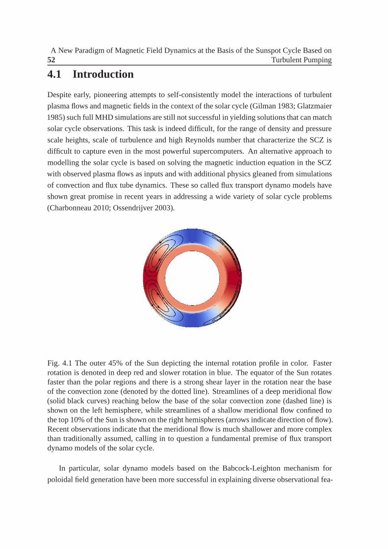
52A New Paradigm of Magnetic Field Dynamics at the Basis of the Sunspot Cycle Based on
Turbulent Pumping
4.1 Introduction
Despite early, pioneering attempts to self-consistently model the interactions of turbulent
plasma flows and magnetic fields in the context of the solar cycle (Gilman 1983; Glatzmaier
1985) such full MHD simulations are still not successful in yielding solutions that can match
solar cycle observations. This task is indeed difficult, forthe range of density and pressure
scale heights, scale of turbulence and high Reynolds numberthat characterize the SCZ is
difficult to capture even in the most powerful supercomputers. An alternative approach to
modelling the solar cycle is based on solving the magnetic induction equation in the SCZ
with observed plasma flows as inputs and with additional physics gleaned from simulations
of convection and flux tube dynamics. These so called flux transport dynamo models have
shown great promise in recent years in addressing a wide variety of solar cycle problems
(Charbonneau 2010; Ossendrijver 2003).
Fig. 4.1 The outer 45% of the Sun depicting the internal rotation profile in color. Fasterrotation is denoted in deep red and slower rotation in blue. The equator of the Sun rotatesfaster than the polar regions and there is a strong shear layer in the rotation near the baseof the convection zone (denoted by the dotted line). Streamlines of a deep meridional flow(solid black curves) reaching below the base of the solar convection zone (dashed line) isshown on the left hemisphere, while streamlines of a shallowmeridional flow confined tothe top 10% of the Sun is shown on the right hemispheres (arrows indicate direction of flow).Recent observations indicate that the meridional flow is much shallower and more complexthan traditionally assumed, calling in to question a fundamental premise of flux transportdynamo models of the solar cycle.
In particular, solar dynamo models based on the Babcock-Leighton mechanism for
poloidal field generation have been more successful in explaining diverse observational fea-
4.2 Results 53
tures of the solar cycle (Dikpati & Charbonneau 1999; Nandy &Choudhuri 2002; Chatterjee
et al. 2004;Choudhuri et al. 2004; Nandy et al. 2011; Choudhuri & Karak 2012, Hazra et al.
2014; Passos et al. 2014). Recent observations also strongly favor the Babcock-Leighton
mechanism as a major source for poloidal field generation (Dasi-Espuig et al. 2010; Muñoz-
Jaramillo et al. 2013). In this scenario, the poloidal field generation is essentially predom-
inantly confined to near-surface layers. For the dynamo to function efficiently, the toroidal
field that presumably resides deep in the interior has to reach the near-surface layers for the
Babcock-Leighton poloidal source to be effective. This is achieved by the buoyant transport
of magnetic flux from the Sun’s interior to its surface (through sunspot eruptions). Subse-
quent to this the poloidal field so generated at near-surfacelayers must be transported back
to the solar interior, where differential rotation can generate the toroidal field. The deep
meridional flow assumed in such models (See Fig. 4.1, left-hemisphere) plays a significant
role in this flux transport process and is thought to govern the period of the sunspot cy-
cle (Charbonneau & Dikpati 2000; Hathaway et al. 2003, Yeates et al. 2008, Hazra et al.
2014). Moreover, a fundamentally crucial role attributed to the deep equatorward merid-
ional flow is that it allows the Parker-Yoshimura sign rule (Parker 1955; Yoshimura 1975)
to be overcome, which would otherwise result in poleward propagating dynamo waves in
contradiction to observations that the sunspot belt migrates equatorwards with the progress
of the cycle (Choudhuri et al. 1995; G.Hazra et al. 2014; Passos et al. 2015; Belusz et al.
2015).
While the poleward meridional flow at the solar surface is well observed (Hathaway
& Rightmire 2010, 2011) the internal meridional flow profile has remained largely uncon-
strained. A recent study utilizing solar supergranules (Hathaway 2012) indicates that the
meridional flow is confined to within the top 10% of the Sun (Fig. 4.1, right-hemisphere)
– much shallower than previously thought. Independent studies utilizing helioseismic in-
versions is also indicative that the equatorward meridional counterflow may be located at
shallow depths (Mitra-Kraev & Thompson 2007; Zhao et al. 2013). The latter also infer
the flow to be multi-cellular and more complex. Here, utilizing a newly developed state-of-
the-art Babcock-Leighton flux transport dynamo model, we explore the impact of a shallow
meridional flow on our current understanding of the solar cycle and provide a new paradigm
which resolves the significant challenges posed by these newobservations.
4.2 Results
Our flux transport solar dynamo model (see chapter 3) solves for the coupled, evolution
equation for the axisymmetric toroidal and poloidal components of the solar magnetic field
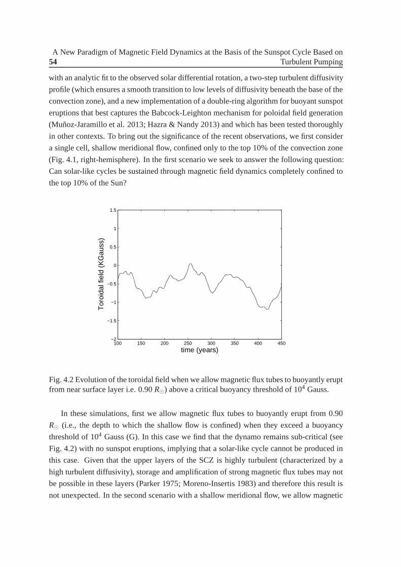
54A New Paradigm of Magnetic Field Dynamics at the Basis of the Sunspot Cycle Based on
Turbulent Pumping
with an analytic fit to the observed solar differential rotation, a two-step turbulent diffusivity
profile (which ensures a smooth transition to low levels of diffusivity beneath the base of the
convection zone), and a new implementation of a double-ringalgorithm for buoyant sunspot
eruptions that best captures the Babcock-Leighton mechanism for poloidal field generation
(Muñoz-Jaramillo et al. 2013; Hazra & Nandy 2013) and which has been tested thoroughly
in other contexts. To bring out the significance of the recentobservations, we first consider
a single cell, shallow meridional flow, confined only to the top 10% of the convection zone
(Fig. 4.1, right-hemisphere). In the first scenario we seek to answer the following question:
Can solar-like cycles be sustained through magnetic field dynamics completely confined to
the top 10% of the Sun?
100 150 200 250 300 350 400 450−2
−1.5
−1
−0.5
0
0.5
1
1.5
time (years)
Tor
oida
l fie
ld (
KG
auss
)
Fig. 4.2 Evolution of the toroidal field when we allow magnetic flux tubes to buoyantly eruptfrom near surface layer i.e. 0.90R⊙) above a critical buoyancy threshold of 104 Gauss.
In these simulations, first we allow magnetic flux tubes to buoyantly erupt from 0.90
R⊙ (i.e., the depth to which the shallow flow is confined) when they exceed a buoyancy
threshold of 104 Gauss (G). In this case we find that the dynamo remains sub-critical (see
Fig. 4.2) with no sunspot eruptions, implying that a solar-like cycle cannot be produced in
this case. Given that the upper layers of the SCZ is highly turbulent (characterized by a
high turbulent diffusivity), storage and amplification of strong magnetic flux tubes may not
be possible in these layers (Parker 1975; Moreno-Insertis 1983) and therefore this result is
not unexpected. In the second scenario with a shallow meridional flow, we allow magnetic
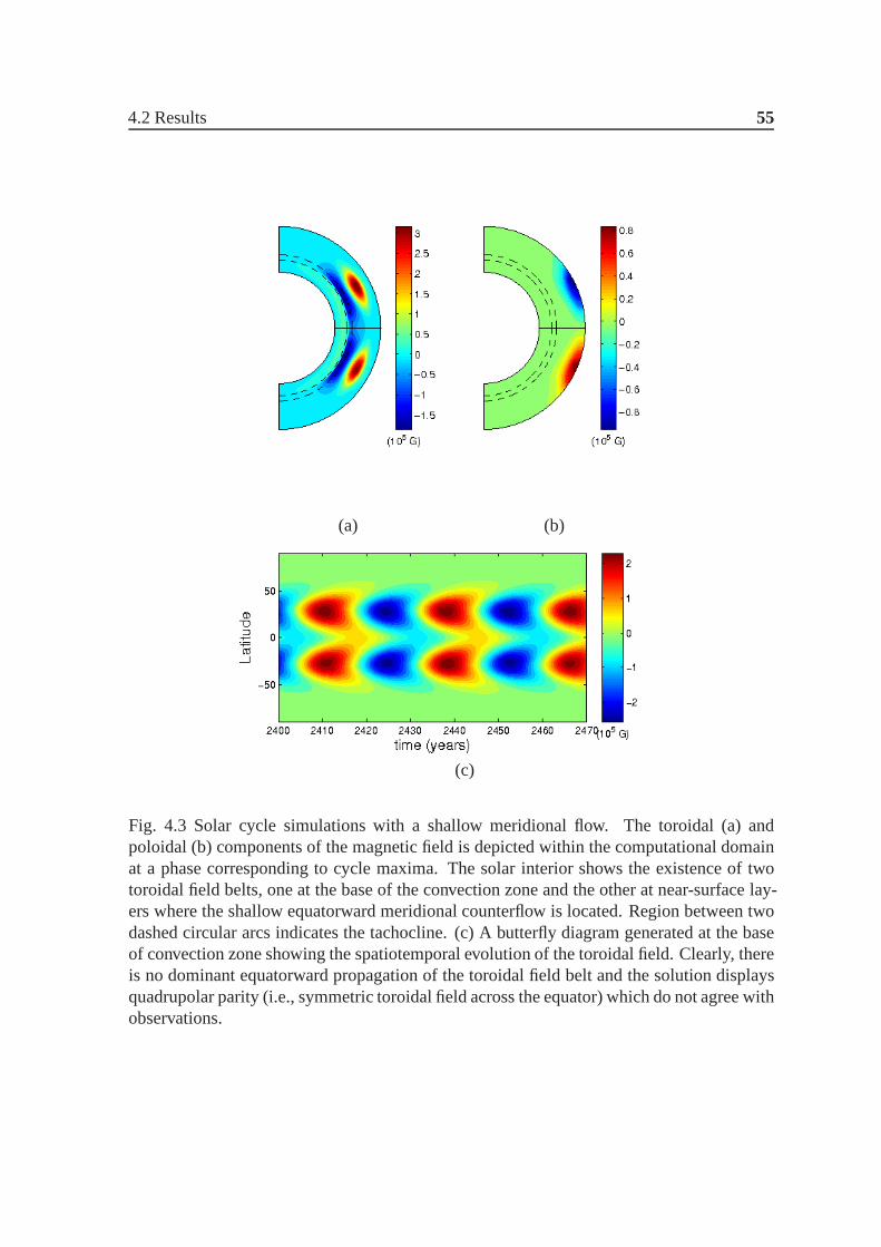
4.2 Results 55
(a) (b)
(c)
Fig. 4.3 Solar cycle simulations with a shallow meridional flow. The toroidal (a) andpoloidal (b) components of the magnetic field is depicted within the computational domainat a phase corresponding to cycle maxima. The solar interiorshows the existence of twotoroidal field belts, one at the base of the convection zone and the other at near-surface lay-ers where the shallow equatorward meridional counterflow islocated. Region between twodashed circular arcs indicates the tachocline. (c) A butterfly diagram generated at the baseof convection zone showing the spatiotemporal evolution ofthe toroidal field. Clearly, thereis no dominant equatorward propagation of the toroidal fieldbelt and the solution displaysquadrupolar parity (i.e., symmetric toroidal field across the equator) which do not agree withobservations.
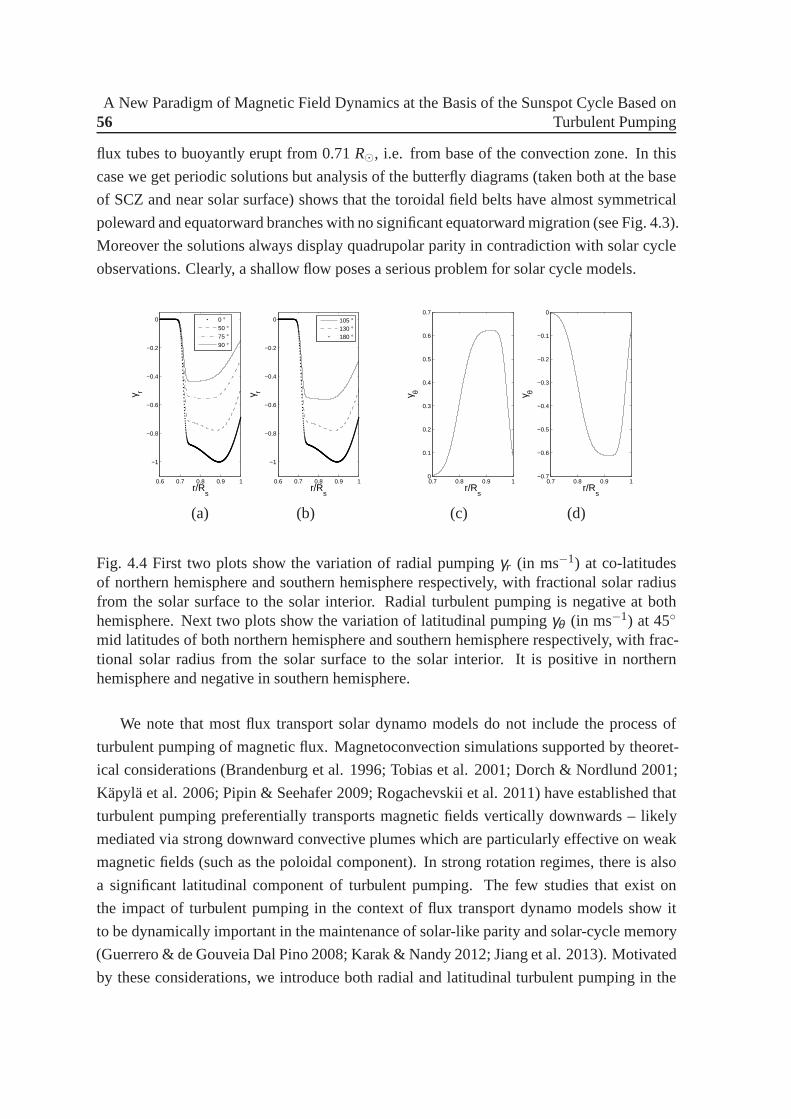
56A New Paradigm of Magnetic Field Dynamics at the Basis of the Sunspot Cycle Based on
Turbulent Pumping
flux tubes to buoyantly erupt from 0.71R⊙, i.e. from base of the convection zone. In this
case we get periodic solutions but analysis of the butterfly diagrams (taken both at the base
of SCZ and near solar surface) shows that the toroidal field belts have almost symmetrical
poleward and equatorward branches with no significant equatorward migration (see Fig. 4.3).
Moreover the solutions always display quadrupolar parity in contradiction with solar cycle
observations. Clearly, a shallow flow poses a serious problem for solar cycle models.
0.6 0.7 0.8 0.9 1
−1
−0.8
−0.6
−0.4
−0.2
0
r/Rs
γ r
0 °50 °75 °90 °
0.6 0.7 0.8 0.9 1
−1
−0.8
−0.6
−0.4
−0.2
0
r/Rs
γ r
105 °130 °180 °
0.7 0.8 0.9 10
0.1
0.2
0.3
0.4
0.5
0.6
0.7
r/Rs
γ θ
0.7 0.8 0.9 1−0.7
−0.6
−0.5
−0.4
−0.3
−0.2
−0.1
0
r/Rs
γ θ
(a) (b) (c) (d)
Fig. 4.4 First two plots show the variation of radial pumpingγr (in ms−1) at co-latitudesof northern hemisphere and southern hemisphere respectively, with fractional solar radiusfrom the solar surface to the solar interior. Radial turbulent pumping is negative at bothhemisphere. Next two plots show the variation of latitudinal pumpingγθ (in ms−1) at 45
mid latitudes of both northern hemisphere and southern hemisphere respectively, with frac-tional solar radius from the solar surface to the solar interior. It is positive in northernhemisphere and negative in southern hemisphere.
We note that most flux transport solar dynamo models do not include the process of
turbulent pumping of magnetic flux. Magnetoconvection simulations supported by theoret-
ical considerations (Brandenburg et al. 1996; Tobias et al.2001; Dorch & Nordlund 2001;
Käpylä et al. 2006; Pipin & Seehafer 2009; Rogachevskii et al. 2011) have established that
turbulent pumping preferentially transports magnetic fields vertically downwards – likely
mediated via strong downward convective plumes which are particularly effective on weak
magnetic fields (such as the poloidal component). In strong rotation regimes, there is also
a significant latitudinal component of turbulent pumping. The few studies that exist on
the impact of turbulent pumping in the context of flux transport dynamo models show it
to be dynamically important in the maintenance of solar-like parity and solar-cycle memory
(Guerrero & de Gouveia Dal Pino 2008; Karak & Nandy 2012; Jiang et al. 2013). Motivated
by these considerations, we introduce both radial and latitudinal turbulent pumping in the
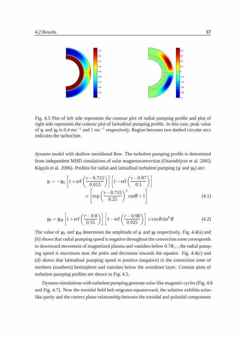
4.2 Results 57
−1
−0.9
−0.8
−0.7
−0.6
−0.5
−0.4
−0.3
−0.2
−0.1
−1
−0.8
−0.6
−0.4
−0.2
0
0.2
0.4
0.6
0.8
Fig. 4.5 Plot of left side represents the contour plot of radial pumping profile and plot ofright side represents the contour plot of latitudinal pumping profile. In this case, peak valueof γr andγθ is 0.4 ms−1 and 1 ms−1 respectively. Region between two dashed circular arcsindicates the tachocline.
dynamo model with shallow meridional flow. The turbulent pumping profile is determined
from independent MHD simulations of solar magnetoconvection (Ossendrijver et al. 2002;
Käpylä et al. 2006). Profiles for radial and latitudinal turbulent pumping (γr andγθ ) are:
γr =−γ0r
[1+erf
(r−0.715
0.015
)][1−erf
(r−0.97
0.1
)]
×[
exp
(r−0.715
0.25
)2
cosθ +1
](4.1)
γθ = γ0θ
[1+erf
(r −0.80.55
)][1−erf
(r −0.980.025
)]×cosθ sin4 θ (4.2)
The value ofγ0r andγ0θ determines the amplitude ofγr andγθ respectively. Fig. 4.4(a) and
(b) shows that radial pumping speed is negative throughout the convection zone corresponds
to downward movement of magnetized plasma and vanishes below 0.7R⊙ , the radial pump-
ing speed is maximum near the poles and decreases towards theequator. Fig. 4.4(c) and
(d) shows that latitudinal pumping speed is positive (negative) in the convection zone of
northern (southern) hemisphere and vanishes below the overshoot layer. Contour plots of
turbulent pumping profiles are shown in Fig. 4.5.
Dynamo simulations with turbulent pumping generate solar-like magnetic cycles (Fig. 4.6
and Fig. 4.7). Now the toroidal field belt migrates equatorward, the solution exhibits solar-
like parity and the correct phase relationship between the toroidal and poloidal components
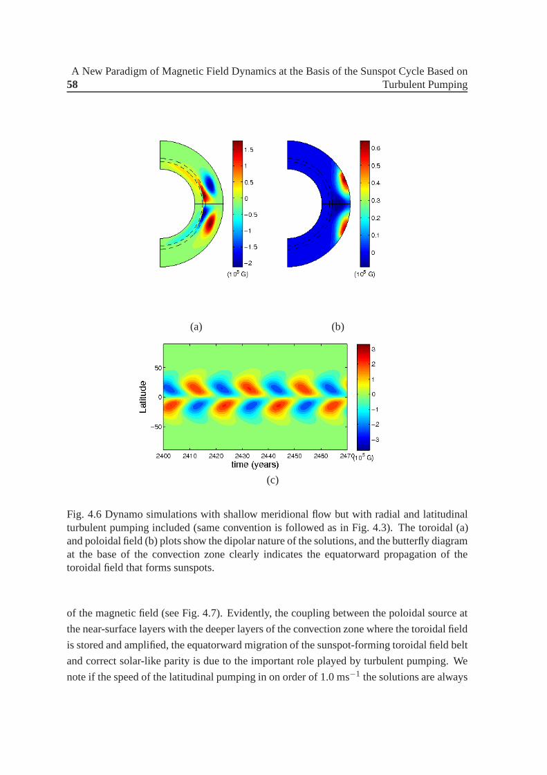
58A New Paradigm of Magnetic Field Dynamics at the Basis of the Sunspot Cycle Based on
Turbulent Pumping
(a) (b)
(c)
Fig. 4.6 Dynamo simulations with shallow meridional flow butwith radial and latitudinalturbulent pumping included (same convention is followed asin Fig. 4.3). The toroidal (a)and poloidal field (b) plots show the dipolar nature of the solutions, and the butterfly diagramat the base of the convection zone clearly indicates the equatorward propagation of thetoroidal field that forms sunspots.
of the magnetic field (see Fig. 4.7). Evidently, the couplingbetween the poloidal source at
the near-surface layers with the deeper layers of the convection zone where the toroidal field
is stored and amplified, the equatorward migration of the sunspot-forming toroidal field belt
and correct solar-like parity is due to the important role played by turbulent pumping. We
note if the speed of the latitudinal pumping in on order of 1.0ms−1 the solutions are always
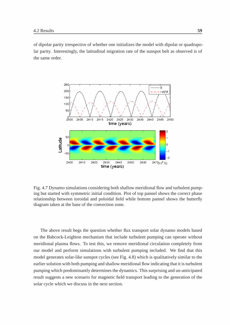
4.2 Results 59
of dipolar parity irrespective of whether one initializes the model with dipolar or quadrupo-
lar parity. Interestingly, the latitudinal migration rateof the sunspot belt as observed is of
the same order.
Fig. 4.7 Dynamo simulations considering both shallow meridional flow and turbulent pump-ing but started with symmetric initial condition. Plot of top pannel shows the correct phaserelationship between toroidal and poloidal field while bottom pannel shows the butterflydiagram taken at the base of the convection zone.
The above result begs the question whether flux transport solar dynamo models based
on the Babcock-Leighton mechanism that include turbulent pumping can operate without
meridional plasma flows. To test this, we remove meridional circulation completely from
our model and perform simulations with turbulent pumping included. We find that this
model generates solar-like sunspot cycles (see Fig. 4.8) which is qualitatively similar to the
earlier solution with both pumping and shallow meridional flow indicating that it is turbulent
pumping which predominantly determines the dynamics. Thissurprising and un-anticipated
result suggests a new scenario for magnetic field transport leading to the generation of the
solar cycle which we discuss in the next section.
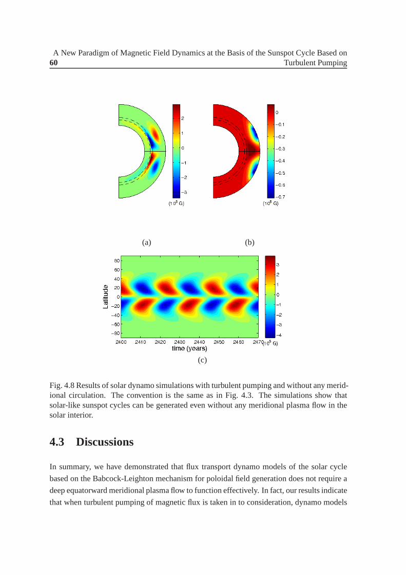
60A New Paradigm of Magnetic Field Dynamics at the Basis of the Sunspot Cycle Based on
Turbulent Pumping
(a) (b)
(c)
Fig. 4.8 Results of solar dynamo simulations with turbulentpumping and without any merid-ional circulation. The convention is the same as in Fig. 4.3.The simulations show thatsolar-like sunspot cycles can be generated even without anymeridional plasma flow in thesolar interior.
4.3 Discussions
In summary, we have demonstrated that flux transport dynamo models of the solar cycle
based on the Babcock-Leighton mechanism for poloidal field generation does not require a
deep equatorward meridional plasma flow to function effectively. In fact, our results indicate
that when turbulent pumping of magnetic flux is taken in to consideration, dynamo models
4.3 Discussions 61
can generate solar-like magnetic cycles even without any meridional circulation. These find-
ings have significant implications for our understanding ofthe solar cycle. First of all, the
serious challenges that was apparently posed by observations of a shallow (and perhaps com-
plex, multi-cellular) meridional flow on the very premise offlux transport dynamo models
stands resolved. Turbulent pumping essentially takes overthe role of meridional circulation
by transporting magnetic fields from the near-surface solarlayers to the deep interior, ensur-
ing that efficient recycling of toroidal and poloidal fields components across the SCZ is not
compromised. While these findings augur well for dynamo models of the solar cycle, they
also imply that we need to revisit many aspects of our currentunderstanding.
It has been argued earlier that the interplay between competing flux transport processes
determine the dynamical memory of the solar cycle governingsolar cycle predictability
(Yeates et al. 2008). If turbulent pumping is the dominant flux transport process as seems
plausible based on the simulations presented herein, the cycle memory would be short and
this is indeed supported by independent studies (Karak & Nandy 2012) and solar cycle obser-
vations (Muñoz-Jaramillo et al. 2013). It is noteworthy that on the other hand, if meridional
circulation were to be the dominant flux transport process, the solar cycle memory would
be relatively longer and last over several cycles. This is not borne out by observations.
Previous results in the context of the maintenance of solar-like dipolar parity have relied
on a strong turbulent diffusion to couple the Northern and Southern hemispheres of the Sun
(Chatterjee et al. 2004), or a dynamoα-effect which is co-spatial with the deep equatorward
counterflow in the meridional circulation assumed in most flux transport dynamo models
(Dikpati & Gilman 2001). However, our results indicate thatturbulent pumping is equally
capable of coupling the Northern and Southern solar hemispheres and aid in the maintenance
of solar-like dipolar parity. This is in keeping with earlier, independent simulations based
on a somewhat different dynamo model (Guerrero & de Gouveia Dal Pino 2008).
Most importantly, our results point out a completely new alternative to circumventing
the Parker-Yoshimura sign rule (Parker 1955; Yoshimura 1975) that would otherwise imply
poleward propagating sunspot belts in conflict with observations of equatorward propaga-
tion of sunspot belt with the progress of the solar cycle. While a deep meridional coun-
terflow is currently thought to circumvent this constraint and force the toroidal field belt
equatorward, our results show that the latitudinal component of turbulent pumping provides
a viable alternative to overcoming the Parker-Yoshimura sign rule.
We note however that our theoretical results should not be taken as support for the exis-
tence of a shallow meridional flow, rather we point out that flux transport dynamo models
of the solar cycle are equally capable for working with a shallow or non-existent meridional
flow, as long as the turbulent pumping of magnetic flux is accounted for. Taken together,

62A New Paradigm of Magnetic Field Dynamics at the Basis of the Sunspot Cycle Based on
Turbulent Pumping
these insights suggest a plausible new paradigm for dynamo models of the solar cycle,
wherein, turbulent pumping of magnetic flux effectively replaces the important roles that
are currently thought to be mediated via a deep meridional circulation within the Sun’s inte-
rior. Since the dynamical memory and thus predictability ofthe solar cycle depends on the
dominant mode of magnetic flux transport in the Sun’s interior, this would also imply that
physics-based prediction models of long-term space weather need to adequately include the
physics of turbulent pumping of magnetic fields.

Chapter 5
Observational Studies of Magnetic Field
Dynamics in the Solar Atmosphere
After discussing the generation process of large scale magnetic fields inside the Sun, in the
second part of this thesis we will concentrate on observations of the photospheric magnetic
field of the Sun and constrain the role of photospheric magnetic fields in atmospheric dy-
namics. Two major explosive events in the solar atmosphere,namely, solar flare and coronal
mass ejection, release huge amounts of plasma to outer space. One of the major outstand-
ing problem in astrophysics is the coronal heating problem:the solar corona is much hotter
compared to the photosphere. In this chapter, we will discuss some observational techniques
and the current theoretical understanding for explaining the observations of the solar atmo-
sphere.
5.1 Measuring large scale solar magnetic field
Zeeman effect is a widely used method to measure solar magnetic fields. In this effect en-
ergy levels of atom split into several levels in presence of static magnetic field (based on
degeneracy of energy level). From the atomic absorption lines interspersed in the black-
body continuum spectra, one can easily choose certain magnetically sensitive lines which
show larger splitting due to their large Lande-g factor. Onecan measure different states
of polarization from these magnetically sensitive lines, in terms of Stokes parameters I, Q,
U, V. The Stokes parameter are used to describe the polarization state of electromagnetic
radiation. These parameters are easily measurable by techniques of remote sensing. Stokes
parameters of a partially polarized light are defined as (Stokes, 1852):

64 Observational Studies of Magnetic Field Dynamics in the Solar Atmosphere
I = l+ ↔ = Ilin(0)+ Ilin(90) = Ix + Iy
Q = l − ↔ = Ilin(0)− Ilin(90) = Ix − Iy
U = ր− ց = Ilin(45)− Ilin(135)
V = − = Icirc(le f t)− Icirc(right)
Stokes I vector represents integrated unpolarized light. Stokes Q parameter represents the
difference between the x and y axis intensities transmittedthrough a polaroid. Parameter U
is the difference between intensities transmitted througha polaroid having axis at 45 and
−45 to the x-axis and parameter V is the difference between between the amount of right
handed circularly polarized light and left handed circularly polarized light present in the
light.
It is possible to determine the strength and direction of magnetic field from the mea-
surement of such polarized signals, using Stokes inversiontechniques (Skumanich & Lites,
1987).
5.2 Effects of large scale solar magnetic field
5.2.1 Null Points and Current Sheet
Null point is the point where all three components of a magnetic field vanishes. It is a
general feature of magnetic fields containing multiple sources, e.g., a field produced by
two bar magnets. Current sheets can form only when the mediumis conducting plasma,
unlike neutral points which can form irrespective of the background medium whether it is
conducting plasma or neutral gas.
A thin current carrying layer across which the magnetic fieldchanges in magnitude or
direction or both, is a current sheet. It has been shown that null points typically give rise
to current sheets in conducting plasma. R. G. Giovanelli (1946) and F. Hoyle (1949) first
suggested that magnetic X-type null points are preferred locations for plasma heating and
initiation of solar flares. T. G. Cowling (1953) pointed out that to power a solar flare, a
current sheet of only few meters thickness is needed. Aroundalmost the same time, J. W.
Dungey (1953) suggested that such current sheets can form bycollapsing magnetic field
lines near an X-type null point.
5.2 Effects of large scale solar magnetic field 65
5.2.2 Magnetic Reconnection
The Magnetic induction equation is given by,
∂B∂ t
= ∇× (v×B)+η∇2B (5.1)
Now the diffusive term is negligible compared to time derivative term if
t << Tdecay=L2
η(5.2)
In that case flux conservation arises because of the balance between the terms∂B∂ t and
∇× (v×B) i.e., magnetic field is coupled within the plasma. This mechanism is easily
applicable for high Reynold’s number plasma system i.e., for astrophysical plasma. So
we can safely assume flux freezing condition as long as evolution time scale (t) is small
compared to diffusion time scale. This flux freezing condition introduces strong constraints
on the dynamics of astrophysical magnetic fields as it implies that connectivity between field
lines can not break and their topology is preserved. We can say, two magnetic configurations
are topologically equivalent if one can be deformed into theother by continuous motion
(without cutting or pasting). But if it is required to cut andpaste field lines, then they are
of different magnetic topology. Now, we can state the flux freezing statement as:In a time
t, magnetic lines of force can slip through the plasma up to the distance l=√
ηt. If our
scale of interest (say,δ ) is very large compared to distancel then flux freezing condition is a
good approximation. However, there are also some situations, when our scale of interest (δ )
is small compared tol in which case this flux freezing condition is no longer valid.In that
case there might be breaking and reattachment between pair of field lines, which is widely
known as magnetic reconnection. Bringing opposing field lines together leads to such large
current densities that there is always break in field lines causing a change in topology even if
the resistivity is very small. These intense thin current layers (also known as current sheet)
are the location for magnetic reconnection.
As topology controls the equilibrium state of the plasma, change in topology corre-
sponds to a change in equilibrium from one configuration to another. On the other hand,
change in equilibrium configuration corresponds to conversion of magnetic energy to other
forms of energy like heat. If this change is sudden then thereis a release of large amounts
of energy. This may be the basis for explosive events in solaratmosphere like solar flares
and coronal mass ejections.
Sweet (1958) and Parker (1957) first quantitatively modelled magnetic reconnection in
two dimension. In their model, they considered the presenceof a thin magnetic diffusion
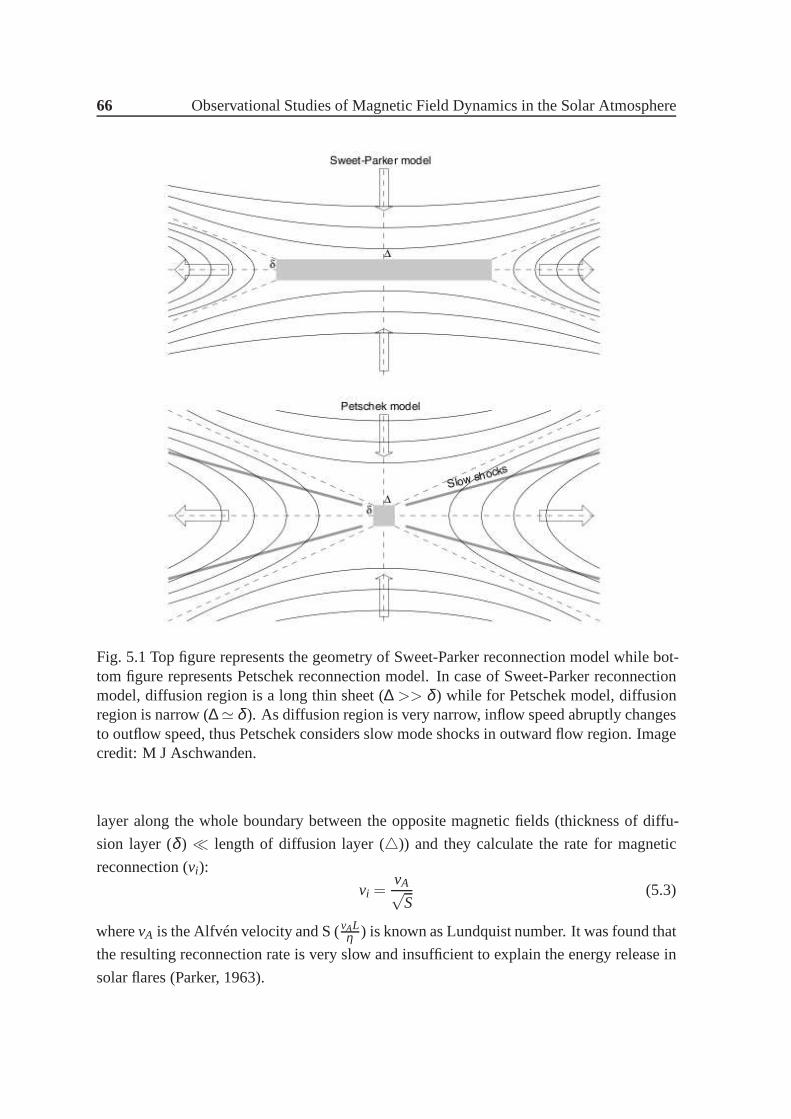
66 Observational Studies of Magnetic Field Dynamics in the Solar Atmosphere
Fig. 5.1 Top figure represents the geometry of Sweet-Parker reconnection model while bot-tom figure represents Petschek reconnection model. In case of Sweet-Parker reconnectionmodel, diffusion region is a long thin sheet (∆ >> δ ) while for Petschek model, diffusionregion is narrow (∆ ≃ δ ). As diffusion region is very narrow, inflow speed abruptly changesto outflow speed, thus Petschek considers slow mode shocks inoutward flow region. Imagecredit: M J Aschwanden.
layer along the whole boundary between the opposite magnetic fields (thickness of diffu-
sion layer (δ ) ≪ length of diffusion layer ()) and they calculate the rate for magnetic
reconnection (vi):
vi =vA√
S(5.3)
wherevA is the Alfvén velocity and S (vALη ) is known as Lundquist number. It was found that
the resulting reconnection rate is very slow and insufficient to explain the energy release in
solar flares (Parker, 1963).

5.2 Effects of large scale solar magnetic field 67
Petschek (1964) came up with a brilliant solution of this problem. As breaking and
reconnection of field lines is a topological process, thus itis only necessary to break and
reconnect field lines near one point. For magnetic reconnection the resistivity of the rest
of the flux system is not important. Thus he reduced the size ofthe diffusion layer to a
narrow area ( ∼ δ ), much less than the length of Sweet-Parker current sheet. As the size
of diffusion region is very narrow, thus plasma inflow speed (let say,v1) abruptly changes
to outflow speed (let say,v2) thus slow-mode shock arises in the Petschek model. Keeping
this in mind, the reconnection rate turns out to be:
vi =vA
log(S)(5.4)
This rate is much faster than Sweet-Parker reconnection rate and is able to explain the energy
released in solar flare like events.
5.2.3 Magnetic Nonpotentiality
The Navier-Stokes equation for incompressible flow can be written as:
ρ∂v∂ t
+ρ(v ·∇)v =−∇p+J×B+ρg+ γ∇2v. (5.5)
when plasma velocity (v) is small, then the Navier-Stokes equation reduces to:
−∇p+J×B+ρg= 0. (5.6)
In case of solar atmosphere, both the pressure gradient (−∇p) and gravitational term (ρg)
are important in the dynamical equilibrium. We can subsume the gravity term in the pressure
term by expressing it as the gradient of a potential; thus total effective pressure is the term
which adjusts itself to equilibrate the Lorentz force. Thuswe can write:
−∇pe f f +J×B = 0. (5.7)
Using the vector identity,∇(A ·B) = A× (∇×B)+B× (∇×A)+(A ·∇)B+B(∇ ·A); we
get:
1µ0
(B ·∇)B = ∇(B2
2µ0+ pe f f). (5.8)

68 Observational Studies of Magnetic Field Dynamics in the Solar Atmosphere
The ratio of gas to magnetic pressure is defined as the plasma-β parameter i.e.,β = 2µ0pB2 .
In case of the solar corona, due to low density the plasma-β is small and one can consider:
J×B = 0. (5.9)
A magnetic field satisfying this condition is known as a force-free field. Now we can satisfy
this condition in three possible ways. First,B = 0 everywhere but we are not interested in
this situation. Second,J = 0 i.e., current vanishes. NowJ = 0 implies∇×B = 0; thus we
can write:
B = ∇φ , (5.10)
whereφ is any scalar potential. This magnetic field configuration isknown as potential
magnetic field or current-free field. Another possibility is:
∇×B = µ0J = α(r)B, (5.11)
whereα(r) is a scalar which is a function of position. Ifα(r) = 0 then current vanishes and
magnetic field corresponds to potential field. But ifα(r) 6= 0 then current does not vanish;
in this case the corresponding magnetic field is known as nonpotential field. So one can take
current as a measure of magnetic nonpotentiality. Using vector identity∇ · (∇×B) = 0, we
can show that:
∇ · (∇×B) = ∇ · (αB) = α(∇ ·B)+B ·∇α = B ·∇α = 0. (5.12)
It indicates thatα does not change along field line. Soα(r) is not a scalar function but a
constant. Magnetic field satisfying condition (5.11) with constantα is known as linear force
free field equation.
If we write the integral form of equation (5.11) with constant α, then we get:
∫
S(∇×B) ·dS=
∫
SαB ·dS So,
∮
CB ·dS=
∫
SαB ·dS (5.13)
The right hand side of the equation isα times the amount of magnetic field passing through
the surface bounded by C while left hand side represents the amount of magnetic field inte-
grated around the circumference of the surface S. Thus relative sizes of these two compo-
nents are indicated by the force-free parameterα, i.e., the amount of twist in the field. This
is the physical significance of the force-free parameterα. The nonpoteniality parameter
represents the departure of the force-free field (observed field in corona) from the potential
field.
5.2 Effects of large scale solar magnetic field 69
To model shear arcades Priest (1982) and Sturrock (1994) considered a loop arcade
which consists of a sequence of loop with a common axis of curvature and generated a
shearing motion by shifting the footpoints parallel to the neutral line on one side along the
solar surface. The shear angle of this arcade is higher when the shearing motion is applied
for longer time. It was shown that:
tanθ =αl, (5.14)
i.e., shear angle (θ ) is proportional toα. So if there is an increase in shear angle, it also
indicates the increase in the nonpotentiality parameterα. Thus shear angle is one of the
major indicator of the magnetic field nonpotentiality.
Now from the study of uniformly twisted, cylindrical, force-free flux tubes (Priest,
1982); it was shown that both force free parameterα and geometric shear angle (i.e., an-
gle between twisted and untwisted field lines) is proportional to the number of twist (say,
Ntwist). Thus one can also use geometric shear angle (θ ) as an estimate of force-free pa-
rameterα. Pevtsov et al. (1997) performed an observational study about the relationship
between geometric shear angle (θ ) and force-free parameterα and found a strong linear
correlation between them. Thus one can measure the nonpotentiality of magnetic field by
measuring shear angle or the twist parameter (α).
5.2.4 Magnetic Helicity
Moreau (1961) and Moffatt (1969) have pointed out that a pseudo scalar quantity called
helicity of the form∫
X · (∇×X)d3x can be related with topological properties of field lines
of ∇×X. Similarly, for magnetic field, one can define magnetic helicity as:
H =∫
B ·A d3x, (5.15)
whereB = ∇×A; A is the vector potential. This quantity is the measure of the linkage
between magnetic field lines.
Woltjer (1958) showed that for a perfectly conducting plasma (ideal MHD, where field
lines are frozen inside the plasma); magnetic helicity is a conserved quantity. He also proved
that, if magnetic helicity is invariant, minimum magnetic energy field configuration always
satisfies the force-free condition i.e.,
∇×B = αB. (5.16)
Taylor (1974) applied this idea to the process of plasma relaxation. He suggested that recon-
nection can remove all topological constraints except total helicity conservation, making the
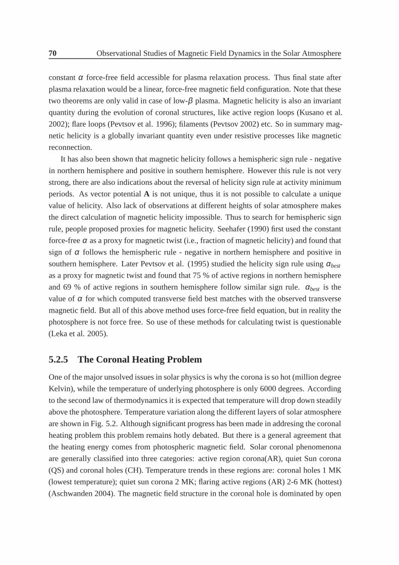
70 Observational Studies of Magnetic Field Dynamics in the Solar Atmosphere
constantα force-free field accessible for plasma relaxation process.Thus final state after
plasma relaxation would be a linear, force-free magnetic field configuration. Note that these
two theorems are only valid in case of low-β plasma. Magnetic helicity is also an invariant
quantity during the evolution of coronal structures, like active region loops (Kusano et al.
2002); flare loops (Pevtsov et al. 1996); filaments (Pevtsov 2002) etc. So in summary mag-
netic helicity is a globally invariant quantity even under resistive processes like magnetic
reconnection.
It has also been shown that magnetic helicity follows a hemispheric sign rule - negative
in northern hemisphere and positive in southern hemisphere. However this rule is not very
strong, there are also indications about the reversal of helicity sign rule at activity minimum
periods. As vector potentialA is not unique, thus it is not possible to calculate a unique
value of helicity. Also lack of observations at different heights of solar atmosphere makes
the direct calculation of magnetic helicity impossible. Thus to search for hemispheric sign
rule, people proposed proxies for magnetic helicity. Seehafer (1990) first used the constant
force-freeα as a proxy for magnetic twist (i.e., fraction of magnetic helicity) and found that
sign of α follows the hemispheric rule - negative in northern hemisphere and positive in
southern hemisphere. Later Pevtsov et al. (1995) studied the helicity sign rule usingαbest
as a proxy for magnetic twist and found that 75 % of active regions in northern hemisphere
and 69 % of active regions in southern hemisphere follow similar sign rule. αbest is the
value ofα for which computed transverse field best matches with the observed transverse
magnetic field. But all of this above method uses force-free field equation, but in reality the
photosphere is not force free. So use of these methods for calculating twist is questionable
(Leka et al. 2005).
5.2.5 The Coronal Heating Problem
One of the major unsolved issues in solar physics is why the corona is so hot (million degree
Kelvin), while the temperature of underlying photosphere is only 6000 degrees. According
to the second law of thermodynamics it is expected that temperature will drop down steadily
above the photosphere. Temperature variation along the different layers of solar atmosphere
are shown in Fig. 5.2. Although significant progress has beenmade in addresing the coronal
heating problem this problem remains hotly debated. But there is a general agreement that
the heating energy comes from photospheric magnetic field. Solar coronal phenomenona
are generally classified into three categories: active region corona(AR), quiet Sun corona
(QS) and coronal holes (CH). Temperature trends in these regions are: coronal holes 1 MK
(lowest temperature); quiet sun corona 2 MK; flaring active regions (AR) 2-6 MK (hottest)
(Aschwanden 2004). The magnetic field structure in the coronal hole is dominated by open
5.2 Effects of large scale solar magnetic field 71
Fig. 5.2 Variation of temperature from solar photosphere tocorona. Spectral lines used forobserving different regions of solar atmosphere are markedat respective locations. Imagecredit: Yang et al. (2009).
magnetic field lines, while in quiet sun and active region corona are mostly closed. In recent
time, theories of coronal heating have been broadly classified into two subcategories– one is
DC heating model i.e., nanoflare heating model, and another is AC heating model i.e., wave
heating theory.
Photospheric drivers, say random motion of magnetic field line footpoints, plausibly
provides the source of energy required for coronal heating.Magnetic disturbances created
by photospheric changes propagate towards corona with the Alfvén speed (vA). In AC heat-
ing model (Wave heating theory), photospheric forcing changes magnetic footpoints rapidly
thereby generating waves. These waves propagate up into thecorona, get dissipated there
and heat the coronal plasma locally. On the other hand, in theDC heating model, pho-
tospheric forcing changes magnetic loop footpoints at timescales much longer than the
Alfvén transit time thus it allows magnetic stresses to build up over time and dissipate in
the corona due to magnetic reconnection, producing heating(Parker 1988). So the basic
problem is to find the exact mechanism which is responsible for coronal heating. In chap-
ter 6 of this thesis, we study the relationship between coronal X-ray intensity and active
region magnetic fields using high resolution Hinode data anddiscuss the consequences of
our results in the context of coronal heating theory.
72 Observational Studies of Magnetic Field Dynamics in the Solar Atmosphere
5.2.6 Solar Flares
A solar flare is an energetic explosive event high up in the solar atmosphere without any
visible energy source. This mystery was resolved when it wasunderstood that it may be pro-
duced by an instability of the underlying magnetic field configuration. Due to this event, the
magnetic field configuration evolves into a more stable stateby changing and reconnecting
the magnetic topology.
Due to the random motions of the magnetic footpoints in the solar photosphere, magnetic
field lines are twisted. Because of this twisted motion, there is a increase in the magnetic
energy much above than the energy of Sun’s vacuum dipole field. Now if a rising bubble
of the magnetic field from the photosphere collides with the twisted magnetic field, then it
produces a reverse field configuration on a very short scale. Then reconnection takes place
in this thin region and lowers the energy of the previous fieldby releasing the twist. In this
way, we can explain solar flare like events. Recent observational studies suggest a close
relation between photospheric magnetic non-potentialityand flare productivity (Jing et al.
2006; Falconer et al. 2008); which may be helpful for predicting solar flares. But a method
of calculating magnetic non-potentiality in terms of twistby using force-free field equation
is questionable as the photosphere is not force free. In chapter 7 of this thesis, we use a
new flux-tube fitting technique to calculate the best-fit twist (Qf it ; one of the measures of
magnetic non-potentiality) and critical twist threshold necessary for determining the suscep-
tibility of magnetic flux tubes to kink instability mechanism (Qkink). We also discuss the
importance of the relationship betweenQf it andQkink for predicting solar flare like events.

Chapter 6
The Relationship between Solar Coronal
X-Ray Brightness and Active Region
Magnetic Fields
In this chapter, using high-resolution observations of nearly co-temporal and co-spatialSo-
lar Optical Telescopespectropolarimeter andX-Ray Telescopecoronal X-ray data onboard
Hinode, we revisit the problematic relationship between global magnetic quantities and coro-
nal X-ray brightness. Co-aligned vector magnetogram and X-ray data were used for this
study. The total X-ray brightness over active regions is well correlated with integrated mag-
netic quantities such as the total unsigned magnetic flux, the total unsigned vertical current
and the area-integrated square of the vertical and horizontal magnetic fields. On account-
ing for the inter-dependence of the magnetic quantities, weinferred that the total magnetic
flux is the primary determinant of the observed integrated X-ray brightness. Our observa-
tions indicate that a stronger coronal X-ray flux is not related to a higher non-potentiality of
active-region magnetic fields. The data even suggest a slight negative correlation between
X-ray brightness and a proxy of active-region non-potentiality. Although there are small
numerical differences in the established correlations, the main results are qualitatively con-
sistent over two different X-ray filters, the Al-poly and Ti-Poly filters, which confirms the
strength of our conclusions and validate and extend earlierstudies that used low-resolution
data. We discuss the implications of our results and the constraints they set on theories of
solar coronal heating.
74The Relationship between Solar Coronal X-Ray Brightness and Active Region Magnetic
Fields
6.1 Introduction
Solar active-region coronal loops appear bright in EUV and X-ray wavelengths, which is
indicative of very high temperatures of the order of a million degrees Kelvin. The ori-
gins behind these high-temperature coronal structures remain elusive. An energy flux of
about 107 ergs cm2 s−1 is required to maintain this high temperature of the coronalplasma
(Withbroe & Noyes 1977). It has been suggested that there is aone-to-one correspondence
between the location of the magnetic fields in the photosphere and bright coronal structures
in the corona (Vaiana et al. 1973) and we know that most of the coronal X-ray luminosity is
concentrated within active-region magnetic-flux systems.
Several theories have been proposed to explain the heating of coronal structures (Zirker
1993; Narain & Ulmschneider 1996; Aschwanden 2004; Klimchuk 2006). These theories
are broadly classified into two subcategories: DC heating model, i.e. the nano-flare heat-
ing model (Parker 1988), and the AC heating model,i.e. the wave-heating theory (e.g. see
the review by Aschwanden, 2004). In the AC heating model, high-frequency MHD waves
are generated in the magnetic foot points of active regions and propagate through magnetic
loops in the corona. These waves dissipate their energy in the corona (Narain & Ulmschnei-
der 1996). Although recent observations reveal that MHD waves propagate into the quiet
solar corona (Tomczyk et al. 2007), it is unclear whether these MHD waves alone can heat
the corona to such a high temperature (Mandrini et al. 2000; Cirtain et al. 2013). Alter-
natively, DC-heating models are proposed to explain the heating of active regions where
nanoflare-like small bursts (each of energy 1024 erg) can liberate energy by magnetic recon-
nection – driven by the constant shuffling of magnetic foot points by turbulent convective
motions just beneath the photosphere (Parker 1988; Cirtainet al. 2013). It has been sug-
gested recently that waves can play a major role in heating the quiet-Sun corona (McIntosh
et al. 2011; Wedemeyer-Böhm et al. 2012), while for coronal active regions the additional
DC heating mechanism must play a role (Parker 1988; Klimchuk2006).
To examine the relative roles of diverse physical mechanisms in the context of coronal
heating, it is essential to have information on the coronal magnetic and velocity field. Cur-
rent instrumentation is still at a nascent stage, however, and is inadequate for such coronal
diagnostics (Lin, Kuhn & Coulter 2004). Since coronal field lines are linked to the pho-
tosphere, another approach is possible: exploring the relationship between photospheric
magnetic-field parameters and brightness of the coronal loops. In earlier studies, Fisher
et al. (1998) and Tan et al. (2007) investigated the relationship between the X-ray lumi-
nosity and photospheric magnetic-field parameters. These two studies reported a strong
correlation between the X-ray luminosity and the total unsigned magnetic flux. Tan et
al. (2007) also found a good correlation between the averageX-ray brightness and aver-
6.1 Introduction 75
age Poynting flux, but ruled out any correlation between the velocity of footpoint motions
and total X-ray brightness. Their computed Poynting flux hada range between 106.7 and
107.6 ergs cm−2 s−1, which is enough to heat the corona (Withbroe & Noyes 1977). Using
data from other wavelengths (UV/EUV channels), Chandrasekhar et al. (2013) also found a
good correlation between total emission from bright pointsand total unsigned photospheric
magnetic flux. Forward-modeling of active regions also suggests a direct correlation be-
tween magnetic flux and X-ray luminosity (Lundquist et al. 2008).
The net current is a measure of non-potentiality of the magnetic field in the active re-
gion. In active-region flare and coronal-mass-ejection processes, the non-potentiality of the
magnetic field can play a significant role (Schrijver et al. 2006; Jing et al. 2006; Wang et
al. 2008). As a result of the low resistivity, large-scale (103 km) currents cannot dissipate
sufficiently in the corona (Hagyard 1988); thus these currents may have no contribution
to coronal heating. Earlier observations do not find a strongrelationship between the to-
tal X-ray luminosity and total vertical current (Metcalf etal. 1994; Fisher et al. 1998).
Note that Wang et al. (2008) showed the existence of 3D current structures over active re-
gions. Another traditionally used measure for magnetic non-potentiality is the parameter
αbestwhich appears in the force-free field equation and which is thought to be related to the
wrapping of magnetic-field lines along the axis of an active-region flux tube (i.e. the twist
of magnetic-field lines). Observation shows that there is nosignificant correlation between
X-ray brightness andαbest(Fisher et al. 1998; Nandy 2008). While many studies have used
αbest as the measure of the twist in the solar active region, this isquestionable because the
photosphere is not deemed to be force-free (Leka et al. 2005). Other studies have shown
that a polarity-inversion line near coronal-loop foot points and strong magnetic shear may
also result in enhanced coronal emission (Falconer 1997; Falconer et al. 1997, 2000).
Longcope (1996) proposed the minimum current corona (MCC) model where coronal
heating was described as a series of small reconnection events punctuating the quasi-static
evolution of coronal field. This model qualitatively predicts the variation of the X-ray lu-
minosity with the total flux that closely matches observations (Fisher et al. 1998). Wang
et al. (2000) have observed bright coronal loops and diffused coronal loops that are asso-
ciated with the quasi-separatrix layers (QSLs). Since QSLsare the places where energy
release occurs through 3D magnetic reconnection, they concluded that QSLs are important
for heating the active-region corona and chromosphere. By analysing the X-ray images
taken fromHinode/X-Ray Telescope(XRT) and correspondingMichelson Doppler Imager
(MDI) line-of-sight magnetograms, Lee et al. (2010) found arelationship between coronal-
loop brightness and magnetic topologies in AR 10963. They also found that frequent tran-
76The Relationship between Solar Coronal X-Ray Brightness and Active Region Magnetic
Fields
sient brightenings in coronal loops are related to separators that have a large amount of free
energy.
Here we revisit the coronal-heating problem with space-based vector-magnetogram data,
which are free from atmospheric seeing effects, which can produce cross talk between var-
ious Stokes parameters. Such space-based magnetic field measurements have also reduced
atmospheric scattered light contribution. The obtained vector-field data are of very high
resolution, thereby reducing the effect of filling factor. In this chapter, we use X-ray images
taken from two filters (Ti-poly and thin Al-poly) of the XRT telescope onboard theHinode
spacecraft and vector magnetic-field measurements taken from theSpectro-Polarimeter(SP)
of Solar Optical Telescope(SOT) to study the relationship between the X-ray brightness and
magnetic-field parameters in active-region flux systems. This study extends previous work
that used lower resolutionYohkohdata (Fisher et al. 1998). We also, incidentally, explore
the effect of the filter response (which is mainly affected bydeposition of unknown ma-
terials on CCD cameras) on the relationship between X-ray brightness and magnetic-field
parameters. In Section 6.2 we provide the details of the dataused in this study. In Section
6.3, we detail our results. In Section 6.4, we discuss the implication of our results for the
heating of the solar corona.
6.2 Data Analysis
6.2.1 Data Selection
The X-ray telescope(XRT: Golub et al. 2007) onboard theHinodespacecraft (Kosugi et
al. 2007) takes images of the solar corona at a spatial resolution of one arcsec per pixel
using different filters. XRT images are of the size 2k×2k pixel, which covers a 34×34
square arcmin field of view (FOV) of the solar corona. XRT observes coronal plasma emis-
sion in the temperature range 5.5 < logT < 8, which is realized by different X-ray filters,
that have their own passband, corresponding to different responses to plasma temperature.
Within a few months of the launch of theHinodespacecraft, contaminating materials were
deposited on the CCD, which significantly impacted the filterresponse, specifically for ob-
servations of longer wavelengths. Regular CCD bakeouts were unable to completely remove
this contamination. As the effect of the contamination is mainly wavelength-dependent (the
long-wavelength observations are affected more strongly), the observations from the thin
Al-poly/Al-mesh filter are more heavily affected than the other filters such as Ti-poly, and
Be-med. For the present study, we have used data taken from Ti-poly and the thin Al-poly
filter, which observe the solar coronal plasma at temperatures higher than 2 MK and 0.5 MK,
6.2 Data Analysis 77
respectively. Therefore, we have a point of comparison to establish whether filter degrada-
tion may play a role in the inconsistencies of the results.
˜ TheSpectro-Polarimeter(SP: Ichimoto et al. 2008) is a separate back-end instrumentof
theSolar Optical Telescope(SOT: Tsuneta et al. 2008) onboard theHinodespacecraft. The
SP provides Stokes signals with high polarimetric accuracyin the 6301 and 6302 Å pho-
tospheric lines. The primary product of the Stokes polarimeter are the Stokes-IQUV pro-
files, which are suitable for deriving the vector magnetic field in the photosphere. The
spatial resolution along the slit direction is 0.295′′ pixel−1; in the scanning direction it is
0.317′′ pixel−1. The Stokes vector was inverted using the MERLIN code, whichis based
on the Milne–Eddington inversion method. The inverted dataprovide the field strength, in-
clination and azimuth along with the Doppler velocity, continuum images, and many other
parameters. The processed data were obtained from the Community Spectropolarimetric
Analysis Center (CSAC). We corrected for the ambiguity in the transverse component of the
magnetic field using the minimum-energy algorithm (Metcalf1994; Leka et al. 2009). The
resulting magnetic-field vectors were transformed into heliographic co-ordinates (Venkatkr-
ishnan and Gary 1989). We selected 40 different NOAA active regions observed at different
times of the year. We also excluded active regions whose central meridional distance was
greater than 30. We took the vector magnetogram data close to the timings of soft X-ray
data obtained from both the Ti-poly and the Al-poly filter of the XRT. In Table 6.1 and 6.2
we list the different active regions used in this study, the date and time of the observations of
the vector magnetogram, and the corresponding soft X-ray data. After these two sets of data,
we also obtained the G-band data taken by theX-Ray Telescope. These data were used for
to co-align each of the data sets. For each selected vector magnetogram, we simultaneously
took XRT X-ray (Ti-poly and Al-poly) data and G-band data. Throughout this chapter, we
use the term Ti-poly dataset to represent the X-ray image obtained from the Ti-poly filter
of XRT onboardHinode. Similarly, we use the term Al-poly for the data taken from the
Al-poly filter. There is always a corresponding vector magnetogram associated with these
data sets. The X-ray data were calibrated using the xrt_prep.pro available in the Solarsoft
routines. The calibrated data were normalized to a one-second exposure time.
6.2.2 Data Coalignment
To overlay the XRT X-ray data with vector magnetograms, we first co-aligned the G-band
data taken by XRT telescope with the continuum image. The continuum image was obtained
by inverting the Stokes data set. To do this, we first identified the dark center of the sunspot
in the G-band and continuum images. Later, we interpolated the continuum image data
to the XRT image resolution. In the next step, we choose the same field of view (FOV)
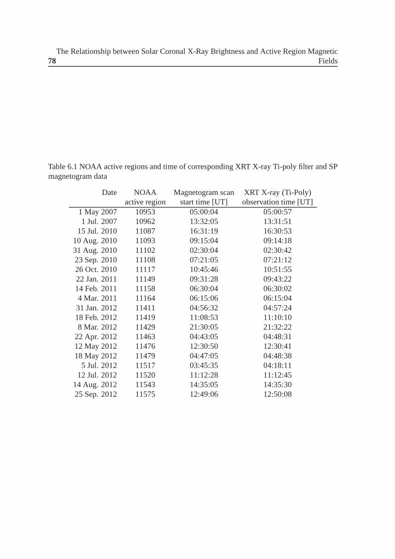
78The Relationship between Solar Coronal X-Ray Brightness and Active Region Magnetic
Fields
Table 6.1 NOAA active regions and time of corresponding XRT X-ray Ti-poly filter and SPmagnetogram data
Date NOAA Magnetogram scan XRT X-ray (Ti-Poly)active region start time [UT] observation time [UT]
1 May 2007 10953 05:00:04 05:00:571 Jul. 2007 10962 13:32:05 13:31:51
15 Jul. 2010 11087 16:31:19 16:30:5310 Aug. 2010 11093 09:15:04 09:14:1831 Aug. 2010 11102 02:30:04 02:30:4223 Sep. 2010 11108 07:21:05 07:21:1226 Oct. 2010 11117 10:45:46 10:51:5522 Jan. 2011 11149 09:31:28 09:43:2214 Feb. 2011 11158 06:30:04 06:30:024 Mar. 2011 11164 06:15:06 06:15:0431 Jan. 2012 11411 04:56:32 04:57:2418 Feb. 2012 11419 11:08:53 11:10:108 Mar. 2012 11429 21:30:05 21:32:22
22 Apr. 2012 11463 04:43:05 04:48:3112 May 2012 11476 12:30:50 12:30:4118 May 2012 11479 04:47:05 04:48:38
5 Jul. 2012 11517 03:45:35 04:18:1112 Jul. 2012 11520 11:12:28 11:12:45
14 Aug. 2012 11543 14:35:05 14:35:3025 Sep. 2012 11575 12:49:06 12:50:08
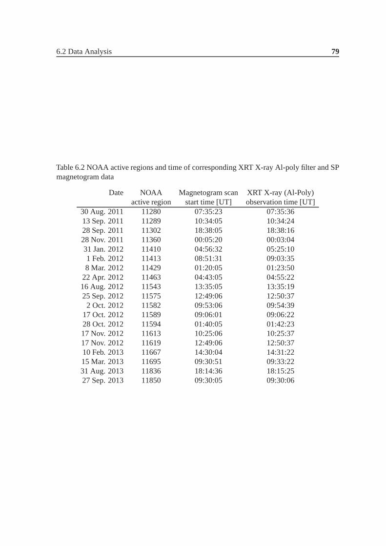
6.2 Data Analysis 79
Table 6.2 NOAA active regions and time of corresponding XRT X-ray Al-poly filter and SPmagnetogram data
Date NOAA Magnetogram scan XRT X-ray (Al-Poly)active region start time [UT] observation time [UT]
30 Aug. 2011 11280 07:35:23 07:35:3613 Sep. 2011 11289 10:34:05 10:34:2428 Sep. 2011 11302 18:38:05 18:38:1628 Nov. 2011 11360 00:05:20 00:03:0431 Jan. 2012 11410 04:56:32 05:25:101 Feb. 2012 11413 08:51:31 09:03:358 Mar. 2012 11429 01:20:05 01:23:50
22 Apr. 2012 11463 04:43:05 04:55:2216 Aug. 2012 11543 13:35:05 13:35:1925 Sep. 2012 11575 12:49:06 12:50:372 Oct. 2012 11582 09:53:06 09:54:39
17 Oct. 2012 11589 09:06:01 09:06:2228 Oct. 2012 11594 01:40:05 01:42:2317 Nov. 2012 11613 10:25:06 10:25:3717 Nov. 2012 11619 12:49:06 12:50:3710 Feb. 2013 11667 14:30:04 14:31:2215 Mar. 2013 11695 09:30:51 09:33:2231 Aug. 2013 11836 18:14:36 18:15:2527 Sep. 2013 11850 09:30:05 09:30:06

80The Relationship between Solar Coronal X-Ray Brightness and Active Region Magnetic
Fields
in the two data sets. By using the maximum-correlation method, we then co-aligned the
continuum images with the G-band images. A similar shift wasapplied to the vector field
data to co-align the entire dataset with X-ray images of the XRT dataset.
6.3 Integrated Quantities
We derived various integrated quantities and compared themwith the X-ray brightness. We
computed the individual as well as integrated quantities such as total magnetic flux, and total
magnetic energyetcand compared them with the X-ray brightness. Below, we describe each
of these quantities.
6.3.1 Active-Region Coronal X-Ray Brightness
The integrated X-ray brightness [Lx] was computed by summing the values of each bright
pixel in the image and then multiplying by the pixel area. Thebright pixels were selected
by using the threshold values. We found the rms value in the X-ray image and selected only
those pixels whose value were higher than the 1-σ level (the rms value) of the image.
6.3.2 Global Magnetic-Field Quantities
Since our selected active regions are close to the disk center, the magnetic-field vectors are
horizontal and vertical to the solar surface. Using theBx, By, andBz components, it is possi-
ble to define the integrated quantities, which can be correlated with the X-ray brightness to
find the relationship between the two (for detailed information about integrated quantities,
see Fisher et al. 1998; Leka et al. 2007). We selected pixels in Bx, By andBz whose values
are greater than the 1-σ level of these images. The following integrated quantitieswere
computed from magnetic field components:
φtot = ∑ |Bz|dA (6.1)
B2z,tot = ∑B2
zdA (6.2)
B2h,tot = ∑B2
hdA (6.3)
Jtot = ∑ |Jz|dA (6.4)
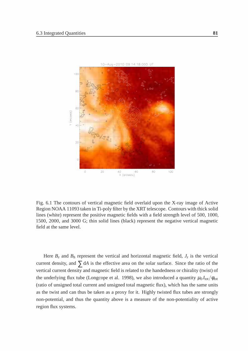
6.3 Integrated Quantities 81
Fig. 6.1 The contours of vertical magnetic field overlaid upon the X-ray image of ActiveRegion NOAA 11093 taken in Ti-poly filter by the XRT telescope. Contours with thick solidlines (white) represent the positive magnetic fields with a field strength level of 500, 1000,1500, 2000, and 3000 G; thin solid lines (black) represent the negative vertical magneticfield at the same level.
HereBz andBh represent the vertical and horizontal magnetic field,Jz is the vertical
current density, and∑dA is the effective area on the solar surface. Since the ratio ofthe
vertical current density and magnetic field is related to thehandedness or chirality (twist) of
the underlying flux tube (Longcope et al. 1998), we also introduced a quantityµ0Jtot/φtot
(ratio of unsigned total current and unsigned total magnetic flux), which has the same units
as the twist and can thus be taken as a proxy for it. Highly twisted flux tubes are strongly
non-potential, and thus the quantity above is a measure of the non-potentiality of active
region flux systems.
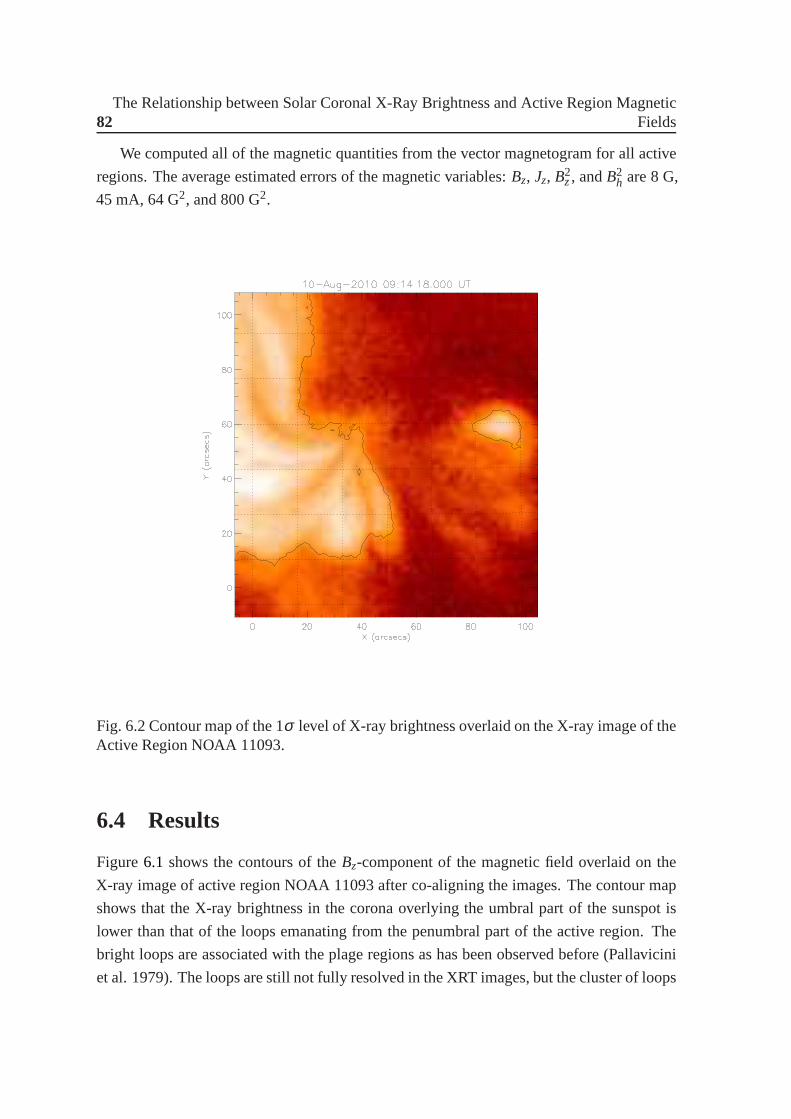
82The Relationship between Solar Coronal X-Ray Brightness and Active Region Magnetic
Fields
We computed all of the magnetic quantities from the vector magnetogram for all active
regions. The average estimated errors of the magnetic variables:Bz, Jz, B2z, andB2
h are 8 G,
45 mA, 64 G2, and 800 G2.
Fig. 6.2 Contour map of the 1σ level of X-ray brightness overlaid on the X-ray image of theActive Region NOAA 11093.
6.4 Results
Figure6.1 shows the contours of theBz-component of the magnetic field overlaid on the
X-ray image of active region NOAA 11093 after co-aligning the images. The contour map
shows that the X-ray brightness in the corona overlying the umbral part of the sunspot is
lower than that of the loops emanating from the penumbral part of the active region. The
bright loops are associated with the plage regions as has been observed before (Pallavicini
et al. 1979). The loops are still not fully resolved in the XRTimages, but the cluster of loops
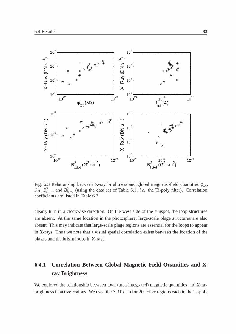
6.4 Results 83
1022
1023
105
106
107
108
φtot
(Mx)
X−
Ray
(D
N s
−1 )
1013
1014
1015
105
106
107
108
Jtot
(A)
X−
Ray
(D
N s
−1 )
1025
1026
104
106
108
B2z,tot
(G2 cm2)
X−
Ray
(D
N s
−1 )
1024
1025
1026
105
106
107
108
B2h,tot
(G2 cm2)
X−
Ray
(D
N s
−1 )
Fig. 6.3 Relationship between X-ray brightness and global magnetic-field quantitiesφtot,Jtot, B2
z,tot, andB2h,tot (using the data set of Table 6.1,i.e. the Ti-poly filter). Correlation
coefficients are listed in Table 6.3.
clearly turn in a clockwise direction. On the west side of thesunspot, the loop structures
are absent. At the same location in the photosphere, large-scale plage structures are also
absent. This may indicate that large-scale plage regions are essential for the loops to appear
in X-rays. Thus we note that a visual spatial correlation exists between the location of the
plages and the bright loops in X-rays.
6.4.1 Correlation Between Global Magnetic Field Quantities and X-
ray Brightness
We explored the relationship between total (area-integrated) magnetic quantities and X-ray
brightness in active regions. We used the XRT data for 20 active regions each in the Ti-poly
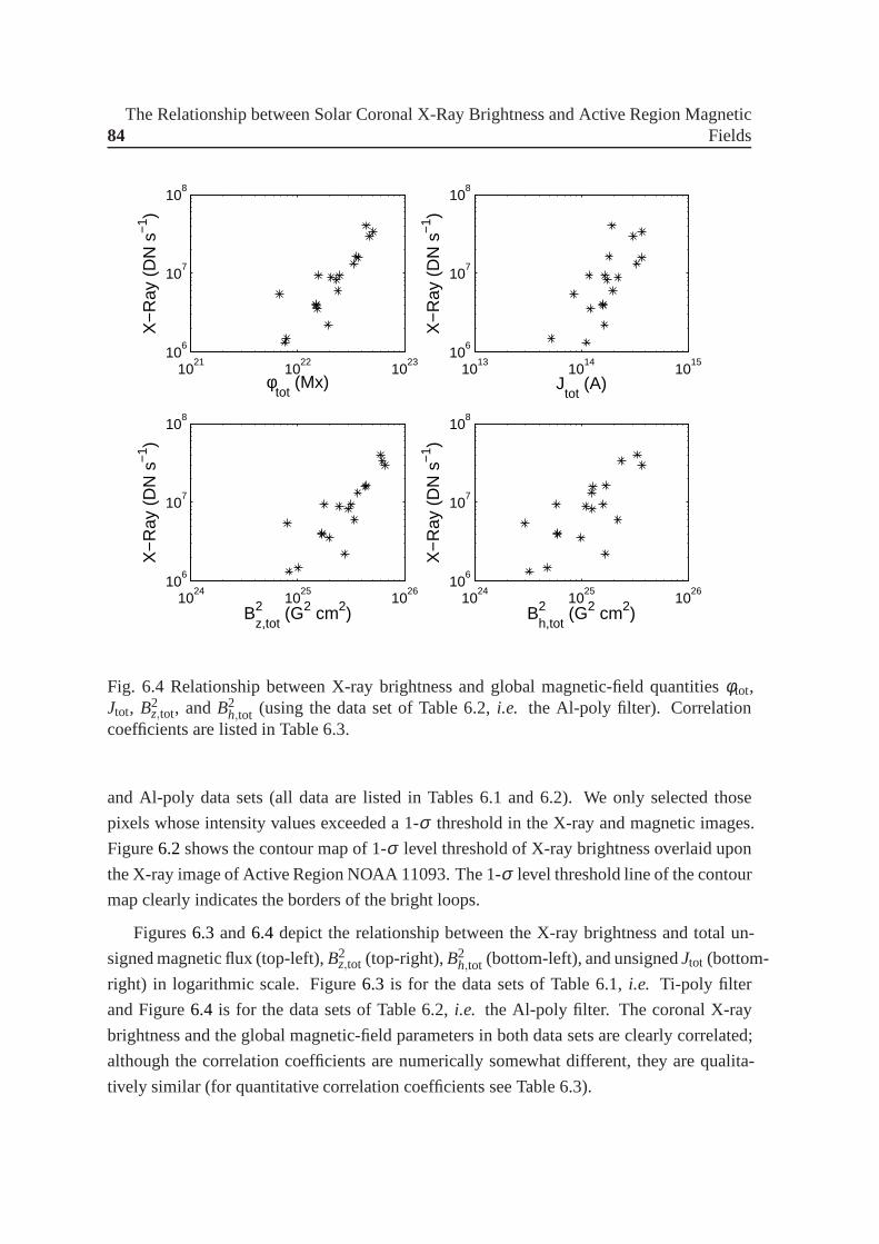
84The Relationship between Solar Coronal X-Ray Brightness and Active Region Magnetic
Fields
1021
1022
1023
106
107
108
φtot
(Mx)
X−
Ray
(D
N s
−1 )
1013
1014
1015
106
107
108
Jtot
(A)
X−
Ray
(D
N s
−1 )
1024
1025
1026
106
107
108
B2z,tot
(G2 cm2)
X−
Ray
(D
N s
−1 )
1024
1025
1026
106
107
108
B2h,tot
(G2 cm2)
X−
Ray
(D
N s
−1 )
Fig. 6.4 Relationship between X-ray brightness and global magnetic-field quantitiesφtot,Jtot, B2
z,tot, andB2h,tot (using the data set of Table 6.2,i.e. the Al-poly filter). Correlation
coefficients are listed in Table 6.3.
and Al-poly data sets (all data are listed in Tables 6.1 and 6.2). We only selected those
pixels whose intensity values exceeded a 1-σ threshold in the X-ray and magnetic images.
Figure6.2shows the contour map of 1-σ level threshold of X-ray brightness overlaid upon
the X-ray image of Active Region NOAA 11093. The 1-σ level threshold line of the contour
map clearly indicates the borders of the bright loops.
Figures6.3 and6.4 depict the relationship between the X-ray brightness and total un-
signed magnetic flux (top-left),B2z,tot (top-right),B2
h,tot (bottom-left), and unsignedJtot (bottom-
right) in logarithmic scale. Figure6.3 is for the data sets of Table 6.1,i.e. Ti-poly filter
and Figure6.4 is for the data sets of Table 6.2,i.e. the Al-poly filter. The coronal X-ray
brightness and the global magnetic-field parameters in bothdata sets are clearly correlated;
although the correlation coefficients are numerically somewhat different, they are qualita-
tively similar (for quantitative correlation coefficientssee Table 6.3).
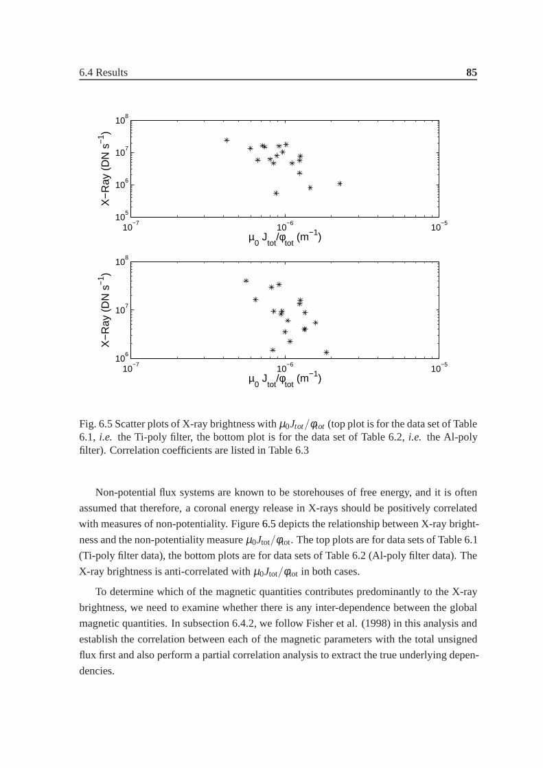
6.4 Results 85
10−7
10−6
10−5
105
106
107
108
µ0 J
tot/φ
tot (m−1)
X−
Ray
(D
N s
−1 )
10−7
10−6
10−5
106
107
108
µ0 J
tot/φ
tot (m−1)
X−
Ray
(D
N s
−1 )
Fig. 6.5 Scatter plots of X-ray brightness withµ0Jtot/φtot (top plot is for the data set of Table6.1, i.e. the Ti-poly filter, the bottom plot is for the data set of Table6.2, i.e. the Al-polyfilter). Correlation coefficients are listed in Table 6.3
Non-potential flux systems are known to be storehouses of free energy, and it is often
assumed that therefore, a coronal energy release in X-rays should be positively correlated
with measures of non-potentiality. Figure6.5depicts the relationship between X-ray bright-
ness and the non-potentiality measureµ0Jtot/φtot. The top plots are for data sets of Table 6.1
(Ti-poly filter data), the bottom plots are for data sets of Table 6.2 (Al-poly filter data). The
X-ray brightness is anti-correlated withµ0Jtot/φtot in both cases.
To determine which of the magnetic quantities contributes predominantly to the X-ray
brightness, we need to examine whether there is any inter-dependence between the global
magnetic quantities. In subsection 6.4.2, we follow Fisheret al. (1998) in this analysis and
establish the correlation between each of the magnetic parameters with the total unsigned
flux first and also perform a partial correlation analysis to extract the true underlying depen-
dencies.
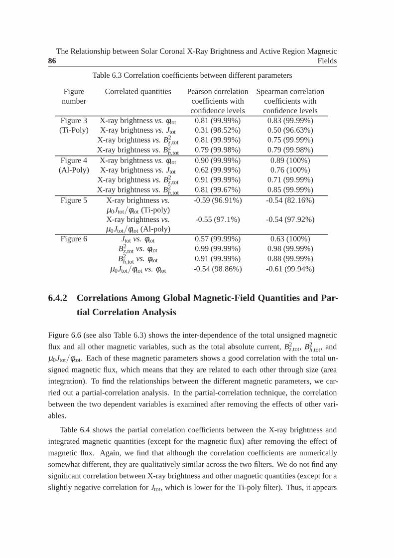
86The Relationship between Solar Coronal X-Ray Brightness and Active Region Magnetic
Fields
Table 6.3 Correlation coefficients between different parameters
Figure Correlated quantities Pearson correlation Spearman correlationnumber coefficients with coefficients with
confidence levels confidence levelsFigure 3 X-ray brightnessvs.φtot 0.81 (99.99%) 0.83 (99.99%)(Ti-Poly) X-ray brightnessvs. Jtot 0.31 (98.52%) 0.50 (96.63%)
X-ray brightnessvs. B2z,tot 0.81 (99.99%) 0.75 (99.99%)
X-ray brightnessvs. B2h,tot 0.79 (99.98%) 0.79 (99.98%)
Figure 4 X-ray brightnessvs.φtot 0.90 (99.99%) 0.89 (100%)(Al-Poly) X-ray brightnessvs. Jtot 0.62 (99.99%) 0.76 (100%)
X-ray brightnessvs. B2z,tot 0.91 (99.99%) 0.71 (99.99%)
X-ray brightnessvs. B2h,tot 0.81 (99.67%) 0.85 (99.99%)
Figure 5 X-ray brightnessvs. -0.59 (96.91%) -0.54 (82.16%)µ0Jtot/φtot (Ti-poly)X-ray brightnessvs. -0.55 (97.1%) -0.54 (97.92%)µ0Jtot/φtot (Al-poly)
Figure 6 Jtot vs.φtot 0.57 (99.99%) 0.63 (100%)B2
z,tot vs.φtot 0.99 (99.99%) 0.98 (99.99%)B2
h,tot vs.φtot 0.91 (99.99%) 0.88 (99.99%)µ0Jtot/φtot vs.φtot -0.54 (98.86%) -0.61 (99.94%)
6.4.2 Correlations Among Global Magnetic-Field Quantities and Par-
tial Correlation Analysis
Figure6.6 (see also Table 6.3) shows the inter-dependence of the totalunsigned magnetic
flux and all other magnetic variables, such as the total absolute current,B2z,tot, B2
h,tot, and
µ0Jtot/φtot. Each of these magnetic parameters shows a good correlationwith the total un-
signed magnetic flux, which means that they are related to each other through size (area
integration). To find the relationships between the different magnetic parameters, we car-
ried out a partial-correlation analysis. In the partial-correlation technique, the correlation
between the two dependent variables is examined after removing the effects of other vari-
ables.
Table6.4 shows the partial correlation coefficients between the X-ray brightness and
integrated magnetic quantities (except for the magnetic flux) after removing the effect of
magnetic flux. Again, we find that although the correlation coefficients are numerically
somewhat different, they are qualitatively similar acrossthe two filters. We do not find any
significant correlation between X-ray brightness and othermagnetic quantities (except for a
slightly negative correlation forJtot, which is lower for the Ti-poly filter). Thus, it appears
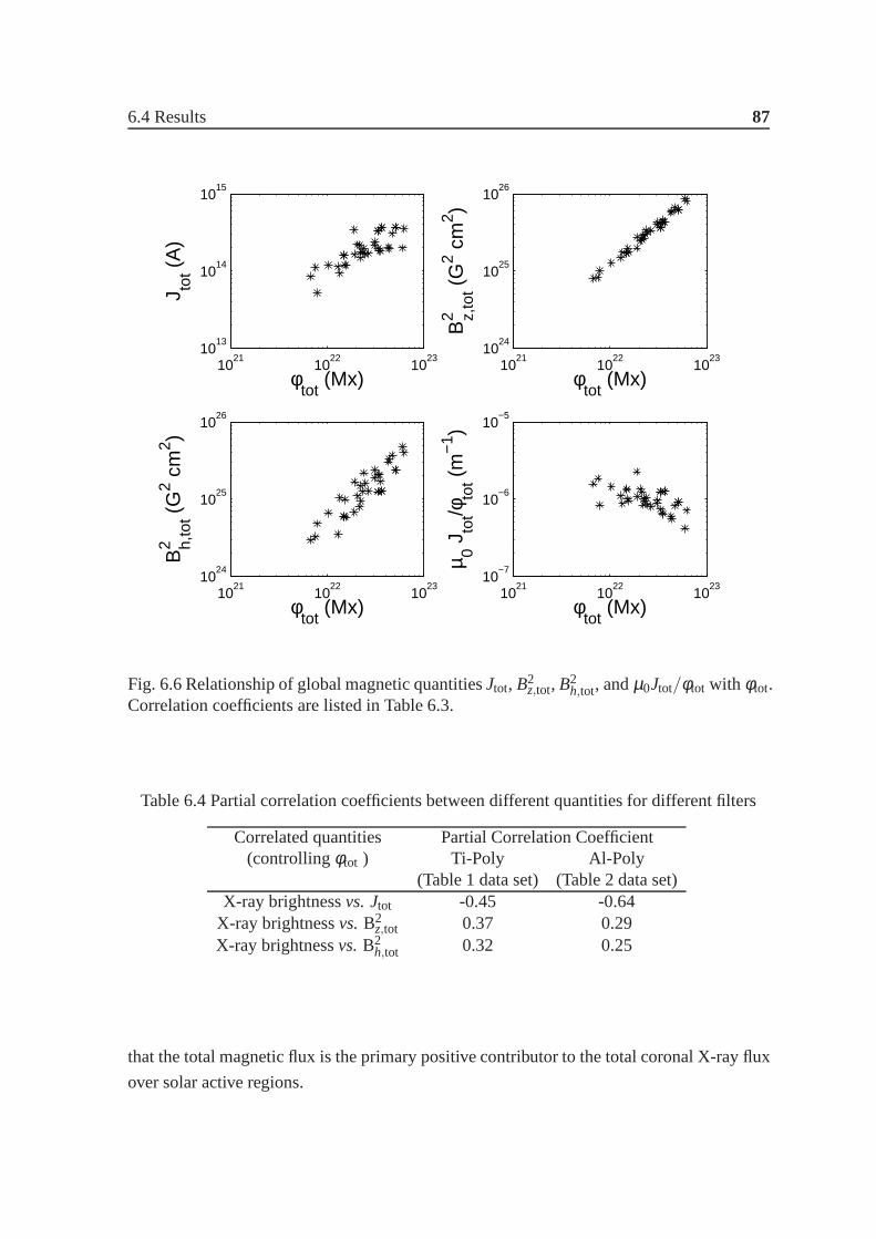
6.4 Results 87
1021
1022
1023
1013
1014
1015
φtot
(Mx)
J tot (
A)
1021
1022
1023
1024
1025
1026
φtot
(Mx)
B2 z,
tot (
G2 c
m2 )
1021
1022
1023
1024
1025
1026
φtot
(Mx)
B2 h,
tot (
G2 c
m2 )
1021
1022
1023
10−7
10−6
10−5
φtot
(Mx)
µ 0 Jto
t/φto
t (m
−1 )
Fig. 6.6 Relationship of global magnetic quantitiesJtot, B2z,tot, B2
h,tot, andµ0Jtot/φtot with φtot.Correlation coefficients are listed in Table 6.3.
Table 6.4 Partial correlation coefficients between different quantities for different filters
Correlated quantities Partial Correlation Coefficient(controllingφtot ) Ti-Poly Al-Poly
(Table 1 data set) (Table 2 data set)X-ray brightnessvs. Jtot -0.45 -0.64
X-ray brightnessvs.B2z,tot 0.37 0.29
X-ray brightnessvs.B2h,tot 0.32 0.25
that the total magnetic flux is the primary positive contributor to the total coronal X-ray flux
over solar active regions.
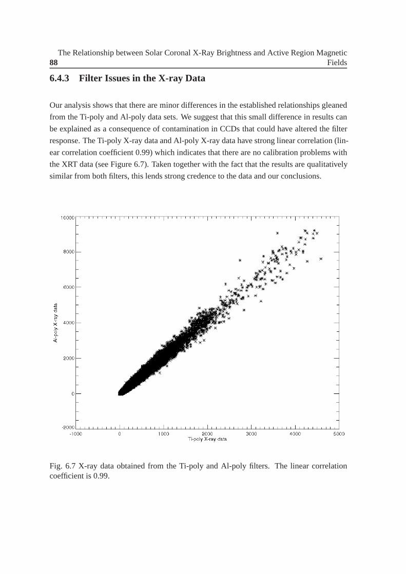
88The Relationship between Solar Coronal X-Ray Brightness and Active Region Magnetic
Fields
6.4.3 Filter Issues in the X-ray Data
Our analysis shows that there are minor differences in the established relationships gleaned
from the Ti-poly and Al-poly data sets. We suggest that this small difference in results can
be explained as a consequence of contamination in CCDs that could have altered the filter
response. The Ti-poly X-ray data and Al-poly X-ray data havestrong linear correlation (lin-
ear correlation coefficient 0.99) which indicates that there are no calibration problems with
the XRT data (see Figure 6.7). Taken together with the fact that the results are qualitatively
similar from both filters, this lends strong credence to the data and our conclusions.
Fig. 6.7 X-ray data obtained from the Ti-poly and Al-poly filters. The linear correlationcoefficient is 0.99.
6.5 Summary and Discussion 89
6.5 Summary and Discussion
A dominant fraction of coronal X-ray emission is known to originate within strongly mag-
netized active-region structures. To establish which of the magnetic-field quantities within
these active regions contributes to the observed X-ray brightness, we have analyzed the X-
ray data from the XRT instrument and vector magnetic field measurements from the SP
instrument onboard theHinodespacecraft. We observed a good correlation between the to-
tal area-integrated magnetic field parameters and the X-raybrightness. A strong correlation
is observed with the total unsigned magnetic flux and closer inspection indicates that other
magnetic parameters are correlated with the X-ray brightness through their dependence on
magnetic flux. This establishes that the magnetic flux (and thus size) of the system matters.
It is generally observed that larger active regions have higher magnetic flux than smaller ac-
tive regions, which suggests that larger active regions arebrighter in X-rays than the small
active regions. This result reconfirms the earlier result ofFisher et al. (1998), which was
based on lower resolution data and is valid across a range of orders of magnitudes across
stars and other astrophysical objects (Pevtsov et al. 2003).
A large amount of total current is indicative of a highly non-potential active region with
a large reservoir of energy. Does this larger energy reservedue to non-potentiality directly
translate into stronger coronal X-ray emission?. Large-scale current systems are known to
produce large-scale flares (Schrijver et al. 2008). It has previously been shown by Nandy
et al. (2003) that the variance in the distribution of the local twist within active-region flux
systems is also an indicator of the flare productivity of active regions. However, even if
this background is suggestive of the role of active region non-potentiality in the release of
energy and one might surmise also in coronal heating, we did not find this to be the case
here. In fact, we found a (weak) negative correlation between X-ray flux and a measure
of non-potentiality, namelyµ0Jtot/φtot. If it does really exist, this correlation has no ob-
vious explanation (at least at this time). Previous studieshave shown that active-region
non-potentiality has a stronger correlation with flare productivity than magnetic flux (Song
et al. 2006; Jing et al. 2006). On the other hand, we found a stronger correlation between X-
ray brightness and unsigned magnetic flux. Thus, one can argue that while non-potentiality
may be an important determinant of localized heating related to flare productivity, the total
unsigned magnetic-flux content is the primary factor governing large-scale coronal heating
over the active regions.
For the Alfvén wave-heating model (e.g. see the review by Aschwanden, 2004), mag-
netic flux is related to the power dissipated at the active region through the square of the
Alfvén velocity, whereas the X-ray brightness would be somefraction of this power – which
also indicates that there should be a relationship between total X-ray brightness and the total

90The Relationship between Solar Coronal X-Ray Brightness and Active Region Magnetic
Fields
magnetic flux. However, based on a detailed analysis, Fisheret al. (1998) showed that the
energy in these waves is not sufficient to explain the observed level of coronal heating. The
MCC model (Longcope 1996) also predicts a strong correlation between total X-ray bright-
ness and total magnetic flux. On the other hand, in the nano-flare heating model (Parker
1988) the power dissipated in active-region coronae is related toB2z,tot, suggesting that the
total X-ray brightness would be strongly correlated withB2z,tot rather thanφtot.
Our observations and analysis suggest that the MCC model is aviable contender as a
physical theory for the heating of solar and stellar coronae. Nevertheless, we note that it is
very likely that a variety of physical processes may contribute to coronal heating to different
extents; there are numerous other subtleties in the coronal-heating problem that are far from
being settled and need further investigations.
Chapter 7
Kink Instability, Coronal Sigmoids and
Solar Eruptive Events
The scientific community is divided on whether the magnetohydrodynamic kink instability
mechanism in highly twisted sunspot magnetic structures can generate solar storms such
as flares and CMEs and form coronal sigmoidal structures. To explore this issue we utilize
high resolution vector magnetograms from the Hinode satellite and a new observational tech-
nique for measuring the twist of photospheric magnetic fields. Following this, we perform
a comparative study of a subset of solar active region magnetic structures, associated flares
and overlying sigmoids or lack thereof, to determine whether the kink instability mecha-
nism can lead to coronal X-ray sigmoids and solar flares. We find that on the rare occasions
that the twist in magnetic structures exceed the kink instability criterion, the active regions
always had a flare associated with them but not necessarily a coronal X-ray sigmoid. Our re-
sults and analysis indicate that kink instability is a plausible source for solar eruptive events
and provides a viable methodology for forecasting solar storms based on this mechanism.
7.1 Introduction
Solar flares and Coronal Mass Ejections (CME) are explosive events responsible for major
disturbances in space weather. It has been well establishedthat solar flares are associated
with sunspots and an analysis of the magnetic structures of active regions (sunspots grouped
together) is necessary to shed more light on the origin of these solar storms.
When a magnetic flux tube rises up through the convection zoneit acquires twist due
to a variety of physical processes including helical turbulence, differential rotation and the
Coriolis force. When this twisted flux tube emerges through the surface of the Sun – the
92 Kink Instability, Coronal Sigmoids and Solar Eruptive Events
photosphere, the magnetic field expands rapidly as background gas pressure decreases, and
overlying coronal loops associated with this active regionare formed and observed in high
energy radiation. The emerged flux tube can be further twisted by shearing photospheric
motions such as foot-point motions and magnetic reconnection. The more a flux tube and
associated magnetic loop is twisted the more it deviates from the potential field condition
(i.e., a current free state) and currents are developed in the system driving it to a higher
energy state. This stressed structure can release the excess energy in the form of solar
flares via magnetic reconnection (Parker 1957, 1963; Petschek 1964; Svestka 1976; Priest
& Forbes 2000; Yokoyama et al. 2001; Takaso et al. 2012; Su et al. 2013; Dudik et al.
2014). However, other alternatives exists for triggering solar eruptive events.
Several observational studies have been performed to explore the relationship between
solar flares and non-potentiality of magnetic fields. These studies find that non-potentiality
of magnetic field is closely linked with the release of solar flares (Tian et al. 2002, Hahn
et al. 2005; Falconer et al. 2008; Jing et al. 2010; Tiwari et al. 2010). One important
parameter used to quantify magnetic non-potentiality is magnetic helicity (which accounts
for both twist and writhe of an isolated flux tube). Theoretical considerations and numerical
simulations show that when the twist of a flux tube exceeds a certain threshold, the flux
tube becomes kink unstable and this instability suddenly converts the twist of the flux tube
to writhe or axial deformation (Linton et al. 1996, 1999). Traditionally, the force free
parameterα – calculated from the force-free field equation∇×B = αB – has been used
as a measure of the twist of solar active regions. The parameter α is roughly equivalent to
twice the magnitude of the twistq. Several methods have been proposed to calculateα, e.g.,
αbest (Pevtsov et al. 1995),αav (Hagino & Sakurai 2004) andαpeak(Leka et al. 2005) from
vector magnetograms. The force free field equation arises from an assumption that the gas
pressure is significantly lesser than the magnetic pressurewhich holds true in the corona.
However the usage of the force free field equation on vector magnetograms is questionable
since the gas pressure in the photosphere is comparable to the magnetic pressure (Metcalf
et al. 1995). To take care of this Nandy et al. (in preparation) proposed a new method
for calculating the twist of photospheric magnetic structures, namely the flux tube fitting
technique method, which does not rely on the force-free fieldassumption.
Leamon et al. (2002) utilized the force-free parameterαbest in an earlier comparative
analysis in a subset of solar active regions to emphaticallystate that kink instability does not
play a role in solar eruptions. However, Fan (2005) used MHD simulations to demonstrate
that a flux tubes can become kink unstable and erupt through the overlying fields if the twist
in the flux tube exceeds a certain value. Leka et al. (2005) performed a blind test on a
single magnetogram using theαpeakmethod proposed in the same paper and suggested that
7.2 Data Selection and Analysis 93
kink instability can be a possible trigger mechanism for solar flares. They argued that the
αbest method underestimates the value of the twist by an order of magnitude as it samples
the whole active region structure. However theαpeak method too suffers from a drawback
– it takes only the peak value of the spatial distribution ofα gleaned from one pixel which
makes it susceptible to errors.
In this chapter, we explicitly test the idea that kink unstable flux tubes are prone to
flaring using the twist calculation method suggested by Nandy et al. (in preparation) which
is free from the shortcomings mentioned above. We provide details about the data used for
our study in Section 7.2. In Section 7.3, we briefly discuss the flux tube fitting technique
developed by Nandy et al. (in preparation) for calculating best-fit twist and critical twist
threshold for kink instability. In Sections 7.4 and 7.5 we proceed to analyse several vector
magnetograms with the said method and present our results and conclusion.
7.2 Data Selection and Analysis
For this study we have used data from the spectro-polarimeter (Ichimoto et al. 2008, SP)
back-end instrument of the solar optical telescope (Tsuneta et al. 2008; SOT) onboard the
Hinode satellite. This instrument measures the stokes signal for spectral lines Fe I 6301
and 6302 Å respectively. It scans the active region in fast scan mode with spatial resolution
0.295′′/pixel−1 (along the slit direction) and 0.317′′/pixel−1 (along the scanning direction)
with a integration time of 1.6 s. Physical magnetic parameters from stokes signal are ob-
tained by inverting the data sets using MERLIN code (based onMilne-Eddington inversion
method) and this inverted data sets are available at the Community Spectro-Polarimeter Cen-
ter (http://sot.lmsal.com/data/sot/level2d and http://www.csac.hao.ucar.edu/). The inherent
180 ambiguity in the transverse field of the vector magnetogram are resolved using the min-
imum energy algorithm (Metcalf 1994; Leka et al. 2009). Thenthe magnetic field vectors
are transformed into heliographic coordinates (Venkatkrishnan & Gary 1989).
For this study, we used 14 different NOAA active regions observed at different times. To
minimize the impact of projection effect on magnetic parameter estimation we select active
regions which lie within a central meridional distance of 30degrees from the disc center.
For this active region data set we subsequently determine whether they had any associ-
ated flares or coronal X-ray sigmoids. Flare information, including timing and class was
taken from the NOAA Flare Catalogue and sigmoidal data was provided by the Hinode X-
Ray Telescope (XRT) Team (see Savcheva et al. 2014). The resulting database of active
regions is detailed in Table 7.1.
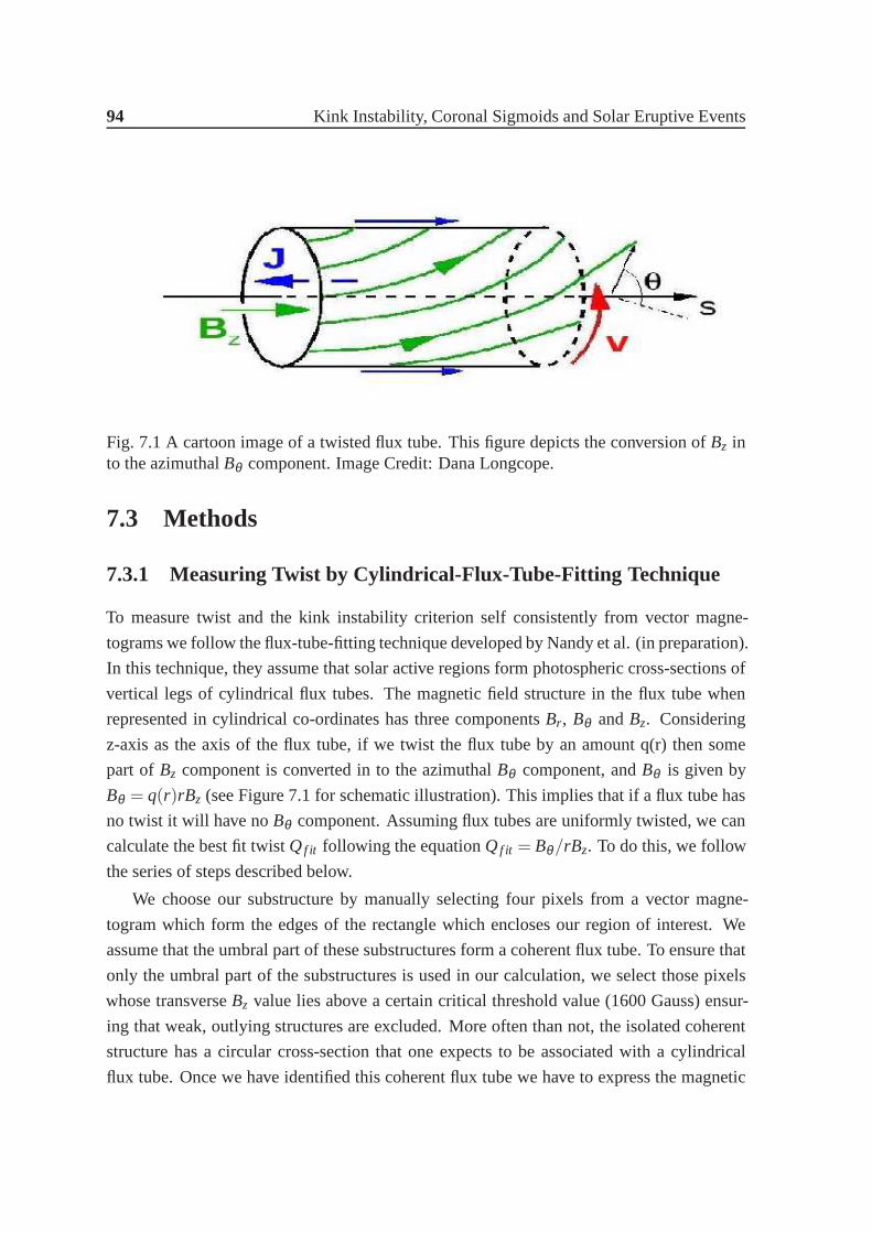
94 Kink Instability, Coronal Sigmoids and Solar Eruptive Events
Fig. 7.1 A cartoon image of a twisted flux tube. This figure depicts the conversion ofBz into the azimuthalBθ component. Image Credit: Dana Longcope.
7.3 Methods
7.3.1 Measuring Twist by Cylindrical-Flux-Tube-Fitting Technique
To measure twist and the kink instability criterion self consistently from vector magne-
tograms we follow the flux-tube-fitting technique developedby Nandy et al. (in preparation).
In this technique, they assume that solar active regions form photospheric cross-sections of
vertical legs of cylindrical flux tubes. The magnetic field structure in the flux tube when
represented in cylindrical co-ordinates has three components Br , Bθ andBz. Considering
z-axis as the axis of the flux tube, if we twist the flux tube by anamount q(r) then some
part of Bz component is converted in to the azimuthalBθ component, andBθ is given by
Bθ = q(r)rBz (see Figure 7.1 for schematic illustration). This implies that if a flux tube has
no twist it will have noBθ component. Assuming flux tubes are uniformly twisted, we can
calculate the best fit twistQf it following the equationQf it = Bθ/rBz. To do this, we follow
the series of steps described below.
We choose our substructure by manually selecting four pixels from a vector magne-
togram which form the edges of the rectangle which encloses our region of interest. We
assume that the umbral part of these substructures form a coherent flux tube. To ensure that
only the umbral part of the substructures is used in our calculation, we select those pixels
whose transverseBz value lies above a certain critical threshold value (1600 Gauss) ensur-
ing that weak, outlying structures are excluded. More oftenthan not, the isolated coherent
structure has a circular cross-section that one expects to be associated with a cylindrical
flux tube. Once we have identified this coherent flux tube we have to express the magnetic
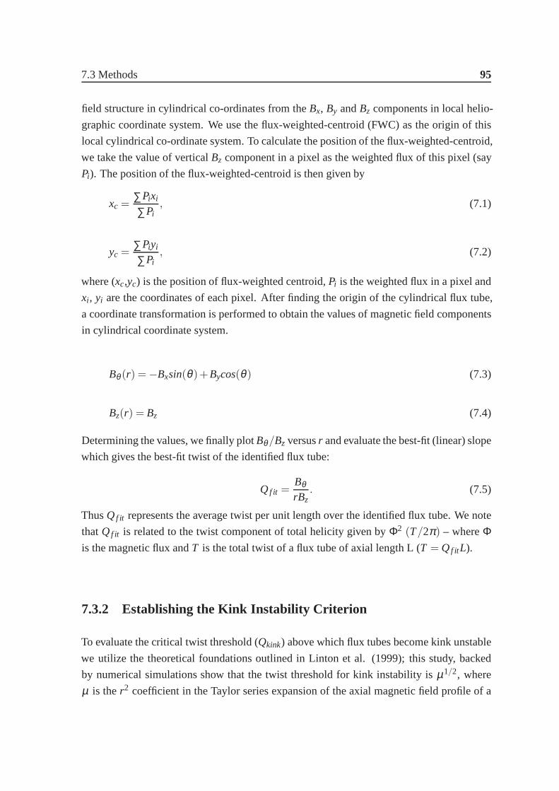
7.3 Methods 95
field structure in cylindrical co-ordinates from theBx, By andBz components in local helio-
graphic coordinate system. We use the flux-weighted-centroid (FWC) as the origin of this
local cylindrical co-ordinate system. To calculate the position of the flux-weighted-centroid,
we take the value of verticalBz component in a pixel as the weighted flux of this pixel (say
Pi). The position of the flux-weighted-centroid is then given by
xc =∑Pixi
∑Pi, (7.1)
yc =∑Piyi
∑Pi, (7.2)
where (xc,yc) is the position of flux-weighted centroid,Pi is the weighted flux in a pixel and
xi , yi are the coordinates of each pixel. After finding the origin ofthe cylindrical flux tube,
a coordinate transformation is performed to obtain the values of magnetic field components
in cylindrical coordinate system.
Bθ (r) =−Bxsin(θ)+Bycos(θ) (7.3)
Bz(r) = Bz (7.4)
Determining the values, we finally plotBθ/Bz versusr and evaluate the best-fit (linear) slope
which gives the best-fit twist of the identified flux tube:
Qf it =BθrBz
. (7.5)
ThusQf it represents the average twist per unit length over the identified flux tube. We note
thatQf it is related to the twist component of total helicity given byΦ2 (T/2π) – whereΦis the magnetic flux andT is the total twist of a flux tube of axial length L (T = Qf it L).
7.3.2 Establishing the Kink Instability Criterion
To evaluate the critical twist threshold (Qkink) above which flux tubes become kink unstable
we utilize the theoretical foundations outlined in Linton et al. (1999); this study, backed
by numerical simulations show that the twist threshold for kink instability is µ1/2, where
µ is ther2 coefficient in the Taylor series expansion of the axial magnetic field profile of a
96 Kink Instability, Coronal Sigmoids and Solar Eruptive Events
Fig. 7.2 Image of AR 10930. Top spot is the negative spot and bottom spot is the positivespot.
cylindrical magnetic flux tube expressed as:
Bz(r) = B0(1−µr2+ ....). (7.6)
HereB0 is the strength of magnetic field along the axis of the flux tube. We plotBz versus
radial distance (r), and perform a fit corresponding to the above equation to determine the
r2 coefficient thereby generating the critical twist threshold:
Qkink = µ1/2. (7.7)
If the flux tube twistQf it exceedsQkink the flux tube will be susceptible to the kink instability
mechanism.
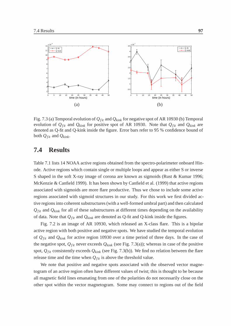
7.4 Results 97
0 5 10 15 20 25 30 35 40 45 50
2
3
4
5
6
7
8
9
10
11
12x 10
−8
time (in hours)
Q−fitQ−kink
0 5 10 15 20 25 30 35 40 45 50
0.5
1
1.5
2
2.5
3
3.5
4
4.5x 10
−7
time (in hours)
Q−fitQ−kink
(a) (b)
Fig. 7.3 (a) Temporal evolution ofQf it andQkink for negative spot of AR 10930 (b) Temporalevolution ofQf it andQkink for positive spot of AR 10930. Note thatQf it andQkink aredenoted as Q-fit and Q-kink inside the figure. Error bars referto 95 % confidence bound ofbothQf it andQkink.
7.4 Results
Table 7.1 lists 14 NOAA active regions obtained from the spectro-polarimeter onboard Hin-
ode. Active regions which contain single or multiple loops and appear as either S or inverse
S shaped in the soft X-ray image of corona are known as sigmoids (Rust & Kumar 1996;
McKenzie & Canfield 1999). It has been shown by Canfield et al. (1999) that active regions
associated with sigmoids are more flare productive. Thus we chose to include some active
regions associated with sigmoid structures in our study. For this work we first divided ac-
tive regions into coherent substructures (with a well-formed umbral part) and then calculated
Qf it andQkink for all of these substructures at different times dependingon the availability
of data. Note thatQf it andQkink are denoted as Q-fit and Q-kink inside the figures.
Fig. 7.2 is an image of AR 10930, which released an X-class flare. This is a bipolar
active region with both positive and negative spots. We havestudied the temporal evolution
of Qf it andQkink for active region 10930 over a time period of three days. In the case of
the negative spot,Qf it never exceedsQkink (see Fig. 7.3(a)); whereas in case of the positive
spot,Qf it consistently exceedsQkink (see Fig. 7.3(b)). We find no relation between the flare
release time and the time whenQf it is above the threshold value.
We note that positive and negative spots associated with theobserved vector magne-
togram of an active region often have different values of twist; this is thought to be because
all magnetic field lines emanating from one of the polaritiesdo not necessarily close on the
other spot within the vector magnetogram. Some may connect to regions out of the field
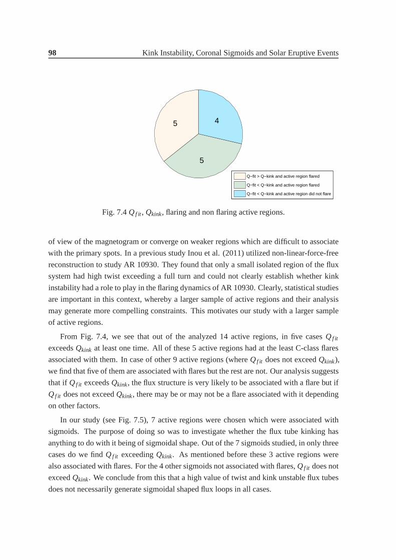
98 Kink Instability, Coronal Sigmoids and Solar Eruptive Events
5
5
4
Q−fit > Q−kink and active region flared
Q−fit < Q−kink and active region flared
Q−fit < Q−kink and active region did not flare
Fig. 7.4Qf it , Qkink, flaring and non flaring active regions.
of view of the magnetogram or converge on weaker regions which are difficult to associate
with the primary spots. In a previous study Inou et al. (2011)utilized non-linear-force-free
reconstruction to study AR 10930. They found that only a small isolated region of the flux
system had high twist exceeding a full turn and could not clearly establish whether kink
instability had a role to play in the flaring dynamics of AR 10930. Clearly, statistical studies
are important in this context, whereby a larger sample of active regions and their analysis
may generate more compelling constraints. This motivates our study with a larger sample
of active regions.
From Fig. 7.4, we see that out of the analyzed 14 active regions, in five casesQf it
exceedsQkink at least one time. All of these 5 active regions had at the least C-class flares
associated with them. In case of other 9 active regions (where Qf it does not exceedQkink),
we find that five of them are associated with flares but the rest are not. Our analysis suggests
that if Qf it exceedsQkink, the flux structure is very likely to be associated with a flarebut if
Qf it does not exceedQkink, there may be or may not be a flare associated with it depending
on other factors.
In our study (see Fig. 7.5), 7 active regions were chosen which were associated with
sigmoids. The purpose of doing so was to investigate whetherthe flux tube kinking has
anything to do with it being of sigmoidal shape. Out of the 7 sigmoids studied, in only three
cases do we findQf it exceedingQkink. As mentioned before these 3 active regions were
also associated with flares. For the 4 other sigmoids not associated with flares,Qf it does not
exceedQkink. We conclude from this that a high value of twist and kink unstable flux tubes
does not necessarily generate sigmoidal shaped flux loops inall cases.
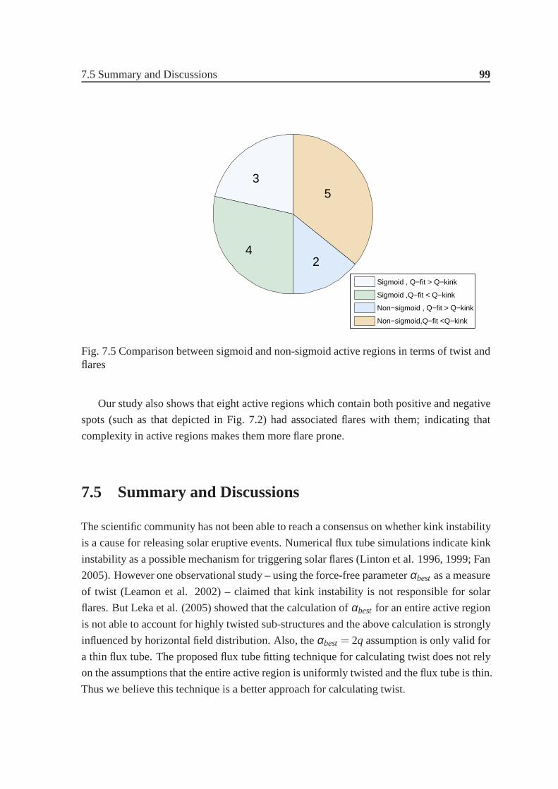
7.5 Summary and Discussions 99
3
4
5
2
Sigmoid , Q−fit > Q−kink
Sigmoid ,Q−fit < Q−kink
Non−sigmoid , Q−fit > Q−kink
Non−sigmoid,Q−fit <Q−kink
Fig. 7.5 Comparison between sigmoid and non-sigmoid activeregions in terms of twist andflares
Our study also shows that eight active regions which containboth positive and negative
spots (such as that depicted in Fig. 7.2) had associated flares with them; indicating that
complexity in active regions makes them more flare prone.
7.5 Summary and Discussions
The scientific community has not been able to reach a consensus on whether kink instability
is a cause for releasing solar eruptive events. Numerical flux tube simulations indicate kink
instability as a possible mechanism for triggering solar flares (Linton et al. 1996, 1999; Fan
2005). However one observational study – using the force-free parameterαbestas a measure
of twist (Leamon et al. 2002) – claimed that kink instabilityis not responsible for solar
flares. But Leka et al. (2005) showed that the calculation ofαbest for an entire active region
is not able to account for highly twisted sub-structures andthe above calculation is strongly
influenced by horizontal field distribution. Also, theαbest= 2q assumption is only valid for
a thin flux tube. The proposed flux tube fitting technique for calculating twist does not rely
on the assumptions that the entire active region is uniformly twisted and the flux tube is thin.
Thus we believe this technique is a better approach for calculating twist.
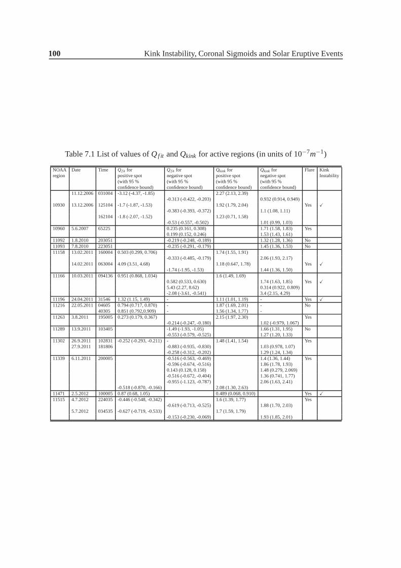
100 Kink Instability, Coronal Sigmoids and Solar Eruptive Events
Table 7.1 List of values ofQf it andQkink for active regions (in units of 10−7m−1)
NOAA Date Time Qf it for Qf it for Qkink for Qkink for Flare Kinkregion positive spot negative spot positive spot negative spot Instability
(with 95 % (with 95 % (with 95 % (with 95 %confidence bound) confidence bound) confidence bound) confidence bound)
11.12.2006 031004 -3.12 (-4.37, -1.85) 2.27 (2.13, 2.39)-0.313 (-0.422, -0.203) 0.932 (0.914, 0.949)
10930 13.12.2006 125104 -1.7 (-1.87, -1.53) 1.92 (1.79, 2.04) Yes X
-0.383 (-0.393, -0.372) 1.1 (1.08, 1.11)162104 -1.8 (-2.07, -1.52) 1.23 (0.71, 1.58)
-0.53 (-0.557, -0.502) 1.01 (0.99, 1.03)10960 5.6.2007 65225 0.235 (0.161, 0.308) 1.71 (1.58, 1.83) Yes
0.199 (0.152, 0.246) 1.53 (1.43, 1.61)11092 1.8.2010 203051 -0.219 (-0.248, -0.189) 1.32 (1.28, 1.36) No11093 7.8.2010 223051 -0.235 (-0.291, -0.179) 1.45 (1.36, 1.53) No11158 13.02.2011 160004 0.503 (0.299, 0.706) 1.74 (1.55, 1.91)
-0.333 (-0.485, -0.179) 2.06 (1.93, 2.17)14.02.2011 063004 4.09 (3.51, 4.68) 1.18 (0.647, 1.78) Yes X
-1.74 (-1.95, -1.53) 1.44 (1.36, 1.50)11166 10.03.2011 094136 0.951 (0.868, 1.034) 1.6 (1.49, 1.69)
0.582 (0.533, 0.630) 1.74 (1.63, 1.85) Yes X
5.43 (2.27, 8.62) 0.314 (0.922, 0.809)-2.08 (-3.61, -0.541) 3.4 (2.15, 4.29)
11196 24.04.2011 31546 1.32 (1.15, 1.49) - 1.11 (1.01, 1.19) - Yes X
11216 22.05.2011 04605 0.794 (0.717, 0.870) - 1.87 (1.69, 2.01) - No40305 0.851 (0.792,0.909) - 1.56 (1.34, 1.77) -
11263 3.8.2011 195005 0.273 (0.179, 0.367) 2.15 (1.97, 2.30) Yes-0.214 (-0.247, -0.180) 1.02 (-0.979, 1.067)
11289 13.9.2011 103405 -1.49 (-1.93, -1.05) 1.66 (1.31, 1.95) No-0.553 (-0.579, -0.525) 1.27 (1.20, 1.33)
11302 26.9.2011 102831 -0.252 (-0.293, -0.211) - 1.48 (1.41, 1.54) Yes27.9.2011 181806 -0.883 (-0.935, -0.830) 1.03 (0.978, 1.07)
-0.258 (-0.312, -0.202) 1.29 (1.24, 1.34)11339 6.11.2011 200005 -0.516 (-0.563, -0.469) 1.4 (1.36, 1.44) Yes
-0.596 (-0.674, -0.516) 1.86 (1.78, 1.93)0.143 (0.128, 0.158) 1.48 (0.279, 2.069)-0.516 (-0.672, -0.404) 1.36 (0.741, 1.77)-0.955 (-1.123, -0.787) 2.06 (1.63, 2.41)
-0.518 (-0.870, -0.166) 2.08 (1.30, 2.63)11471 2.5.2012 100005 0.87 (0.68, 1.05) - 0.489 (0.068, 0.910) Yes X
11515 4.7.2012 224035 -0.446 (-0.548, -0.342) 1.6 (1.39, 1.77) Yes-0.619 (-0.713, -0.525) 1.88 (1.70, 2.03)
5.7.2012 034535 -0.627 (-0.719, -0.533) 1.7 (1.59, 1.79)-0.153 (-0.230, -0.069) 1.93 (1.85, 2.01)
7.5 Summary and Discussions 101
Here we have studied the susceptibility of active region fluxtubes to the kink instabil-
ity mechanism using this new flux tube fitting technique for calculating twist. Using this
technique, we find that if the best fit twist (Qf it ) of any active region exceeds the threshold
necessary for kink instability a flare is always associated with this active region. On the
other hand, we also find some active regions where best-fit twist does not exceed the kink
instability threshold which had flares associated with them. On another front, Rust & Ku-
mar (1996) suggested that sigmoids are kink unstable twisted flux tubes. We do not find
this to be the case. Within our seven sigmoid data set, we find only three sigmoids had kink
unstable (photospheric) flux tubes associated with them.
In summary, we conclude that kink instability is the cause for at least a subset of solar
flares but the corresponding active regions need not have coronal sigmoidal structures associ-
ated with them. This result and the analysis outlined here may form the basis of forecasting
solar flares in advance when accurate vector magnetogram measurements are available.

Appendix A
Numerical Methods
We provide a overview of numerical methods which is used to solve dynamo equations in
a two dimensional geometry. The evolution equation for the poloidal and toroidal field is
given by:∂A∂ t
+1s[vp ·∇(sA)] = η
(∇2− 1
s2
)A+S(r,θ ,B), (A.1)
∂B∂ t
+s
[vp ·∇
(Bs
)]+(∇ ·vp)B= η
(∇2− 1
s2
)B+s
([∇× (Aeφ )
]·∇Ω
)+
1s
∂ (sB)∂ r
∂η∂ r
,
(A.2)
wheres= r sin(θ). These two equations are coupled, nonlinear partial differential equation.
We solve these equations as a intial value problem using Alternating Direction Implicit
(ADI) method (Press et al. 1988). In this method, we write these equations in operator
splitting method:∂A∂ t
= [Lr +Lθ ]A+Sp, (A.3)
∂B∂ t
= [Nr +Nθ ]B+St , (A.4)
whereLr andNr are the operators involving r-derivative; similarlyLθ andNθ are the op-
erators involvingθ derivatives.Sp andSt (rotational shear term) are the source terms for
the poloidal and toroidal field respectively. In our model,St = s([
∇× (Aeφ )]·∇Ω
)i.e.,
source term for toroidal field andSp = S(r,θ ,B), i.e., source term for poloidal field due to
the Babcock-Leighton mechanism which is modelled by doublering algorithm.
From equation (A.1), the operatorsLr andLθ is given by:
LrA=−vr
r∂∂ r
(rA)+η[
∂ 2A∂ r2 +
2r
∂A∂ r
− A2r2sin2θ
], (A.5)
104 Numerical Methods
Lθ A=− vθrsinθ
∂∂θ
(Asinθ)+η[
1r
∂ 2A∂θ2 +
cotθr2
∂A∂θ
− A2r2sin2θ
]. (A.6)
Here we describe the basic theme of Alternating Direction Implicit (ADI) method in
case of two dimensional system. In Alternating Direction Implicit (ADI) method, each time
step is divided into two half time steps for two dimensional geometry. In the first half time
step, one direction (say r), is advanced implicitly then other direction (sayθ ) is advanced
explicitly. In the second half step,θ direction is advanced implicitly and r direction is
advanced explicitly. Let the value of A at grid point (i,j) attime step m isAmi, j . Then the ADI
scheme consists of following two time steps:
Am+ 1
2i, j −Am
i, j = (LrAm+ 1
2i, j +Lθ Am
i, j)∆t2
(A.7)
Am+1i, j −A
m+ 12
i, j = (LrAm+ 1
2i, j +Lθ Am+1
i, j )∆t2
(A.8)
HereLr andLθ represent the difference forms of the operatorsLr andLθ .
Here we treat the diffusion term by Crank-Nicholson scheme.We use an first order accurate
upwind scheme to treat the terms∂A∂ r and∂A
∂θ . The hyperbolic advective terms [−vrr
∂∂ r (rA)] is
handled by Lax-Wendroff scheme, which is second order accurate in time and avoids mesh
drifting, large numerical dissipation.
Treating various terms in this way, we get the following forms ofLr andLθ :
LrAmi, j = d(i, j)Am
i−1, j +e(i, j)Ami, j + f (i, j)Am
i+1, j (A.9)
Lθ Ami, j = a(i, j)Am
i, j−1+b(i, j)Ami, j +c(i, j)Am
i, j+1 (A.10)
The matrix coefficients can be calculated with straight forward algebra and take the form:
a(i, j) =η
(r∆θ)2 +Uθ (i, j)
∆θsin(θ − ∆θ
2)
[12+
∆t4∆θ
Uθ (i, j − 12)sin(θ −∆θ)
](A.11)
105
b(i, j) =− 2η(r∆θ)2 −
ηcotθr2∆θ
− η2r2sin2θ
−Uθ (i, j)∆θ
[sin(θ +
∆θ2)
12+
∆t4∆θ
Uθ (i, j +12)sinθ
−sin(θ − ∆θ
2)
12− ∆t
4∆θUθ (i, j − 1
2)sinθ
](A.12)
c(i, j) =η
(r∆θ)2 +ηcotθr2∆θ
− Uθ (i, j)∆θ
sin(θ +∆θ2)
[12− ∆t
4∆θUθ (i, j +
12)sin(θ +∆θ)
]
(A.13)
d(i, j) =η
(∆r)2 +Ur(i, j)
∆r(r − ∆r
2)
[12+
∆t4∆r
Ur(i −12, j)(r −∆r)
](A.14)
e(i, j) =− 2η(∆r)2 −
2ηr∆r
− η2r2sin2θ
−Ur(i, j)∆r[
∆r2
+∆t
4∆rr
Ur(i +
12, j)(r +
∆r2)+Ur(i −
12, j)(r − ∆r
2)
](A.15)
f (i, j) =η
(∆r)2 +2ηr∆r
− Ur(i, j)∆r
(r +∆r2)
[12− ∆t
4∆rUr(i +
12, j)(r +∆r)
](A.16)
HereUr(i, j) andUθ (i, j) give the values ofvrr and vθ
rsinθ at the grid point (i,j).
Using (A.9) and (A.10), we can write the equation (A.7) in theform:
a(i, j)Am+ 1
2i, j−1+[1+b(i, j)]A
m+ 12
i, j +c(i, j)Am+ 1
2i, j+1 = Ψ(i, j), (A.17)
where,
Ψ(i, j) =−d(i, j)Ami−1, j +[1−e(i, j)]Am
i, j − f (i, j)Ami+1, j . (A.18)
Similarly in second step of ADI method, we can write the equation (A.8) in the form:
d(i, j)Am+1i−1, j +[1+e(i, j)]Am+1
i, j + f (i, j)Am+1i+1, j = Φ(i, j), (A.19)

106 Numerical Methods
where,
Φ(i, j) =−a(i, j)Am+ 1
2i, j−1+[1−b(i, j)]A
m+ 12
i, j −c(i, j)Am+ 1
2i, j+1
=−Ψ(i, j)+2Am+ 1
2i, j . (A.20)
The coefficients of all these equations form a tridiagonal matrix. Source term (Sp) is
treated explicitly in the code. In the first half step of ADI method, we solve the equation
(A.17) and get the values ofAm+ 1
2i, j at all grid points. In the second half step, we solve the
equation (A.19), and get the values ofAm+1i, j at all grid points.
Similarly, we can solve the toroidal field evolution equation. In case of the toroidal field
evolution equation, For first half step of ADI method,
ab(i, j)Bm+ 1
2i, j−1+[1+bb(i, j)]B
m+ 12
i, j +cb(i, j)Bm+ 1
2i, j+1 = χ(i, j), (A.21)
where,
χ(i, j) =−db(i, j)Bmi−1, j +[1−eb(i, j)]Bm
i, j − f b(i, j)Bmi+1, j . (A.22)
and for second half step of ADI method:
db(i, j)Bm+1i−1, j +[1+eb(i, j)]Bm+1
i, j + f b(i, j)Bm+1i+1, j = Γ(i, j), (A.23)
where,
Γ(i, j) =−ab(i, j)Bm+ 1
2i, j−1+[1−bb(i, j)]B
m+ 12
i, j −cb(i, j)Bm+ 1
2i, j+1
=−χ(i, j)+2Bm+ 1
2i, j . (A.24)
The expression for the matrix coefficients necessary for thetoroidal field evolution equa-
tion are given by:
ab(i, j)=η
(r∆θ)2 +Uθ (i, j − 1
2)
∆θsin(θ− ∆θ
2)
[12+
∆t4∆θ
Uθ (i, j −1)sin(θ −∆θ)]
(A.25)
107
bb(i, j) =− 2η(r∆θ)2 −
ηcotθr2∆θ
− η2r2sin2θ
−[
Uθ (i, j + 12)
∆θsin(θ +
∆θ2)
12+
∆t4∆θ
Uθ (i, j)sinθ−Uθ (i, j − 1
2)
∆θsin(θ − ∆θ
2)
12− ∆t
4∆θUθ (i, j)sinθ
](A.26)
cb(i, j)=η
(r∆θ)2+ηcotθr2∆θ
−Uθ (i, j + 12)
∆θsin(θ +
∆θ2)
[12− ∆t
4∆θUθ (i, j +1)sin(θ +
∆θ2)
]
(A.27)
db(i, j) =η
(∆r)2 +U r(i, j)
∆r(r − ∆r
2)
[12+
∆t4∆r
U r(i −12, j)(r −∆r)
](A.28)
eb(i, j) =− 2η(∆r)2 −
2ηr∆r
− η2r2sin2θ
−U′r(i, j)−U r(i, j)
∆r[∆r2
+r∆t4∆r
U r(i +
12, j)(r +
∆r2)+U r(i −
12, j)(r − ∆r
2)
](A.29)
f b(i, j) =η
(∆r)2 +η
r∆r− U r(i, j)
∆r(r +
∆r2)
[12− ∆t
4∆rU r(i +
12, j)(r +
∆r2)
](A.30)
where,U r =Ur− dη
drr .
We solve these equations in an×n grid with the appropriate initial and boundary condi-
tions.

References
Alfvén, H. 1942, Ark. f. Mat. Astr. o. Fysik., 29B, No. 2
Antiochos, S.K., Dahlburg, R.B. & Klimchuk, J.A. 1994, ApJL, 420, L41
Arlt, R. & Abdolvand, A. 2010, in Physics of Sun and Star Spots, Proceedings IAU Sympo-
sium No. 273, ed. D.P. Choudhary & K.G. Strassmeier.
Aschwanden, M.: 2004,Physics of the Solar Corona, An Introduction, Springer, Praxis
Publishing, Chichester, UK.
Babcock, H. W. & Babcock, H. D. 1955, ApJ, 121, 349
Babcock, H. W. 1959, ApJ, 130, 364
Babcock, H. W. 1961, ApJ, 133, 572
Barker, A.J., Silvers, L.J., Proctor, M.R.E. & Weiss, N.O. 2012, MNRAS, 424,115
Barnes, G., Longcope, D. W. & Leka, K. D. 2005, ApJ, 629, 561
Beer, J., Tobias, S.M. & Weiss, N. 1998, SoPh, 181, 23
Belucz, B., Dikpati, M. & Forgacs-Dajka, N. 2015, ApJ, 806, 169
Bonanno, A., Elstner, D., Rüdiger, G., & Belvedere, G. 2002,A&A, 390, 673
Bonanno, A., Elstner, D., Belvedere, G., & Rüdiger, G. 2006,Memorie della Societa Astro-
nomica Italiana Supplementi, 9, 71
Braun, D. C. & Fan, Y. 1998, ApJ, 508, L105
Brandenburg, A., Moss, D., & Tuominen, I. 1992, in Astronomical Society of the Pacific
Conference Series, Vol. 27, The Solar Cycle, ed. K. L. Harvey, 536–+
110 References
Brandenburg, A., Jennings, R.L., Nordlund, A., Rieutord, M., Stein, R.M., Tuominen, I.
1996, JFM, 306, 325
Brown, B.P., Browning, M.K., Brun, A.S., Miesch, M.S. & Toomre, J. 2010, ApJ, 711, 424
Bushby, P. J., & Tobias, S. M. 2007, ApJ, 661, 1289
Caligari, P., Moreno-Insertis, F. & Schüssler, M. 1995 , ApJ, 441, 886.
Caligari, P.,Schüssler, M. & Moreno-Insertis, F. 1998 , ApJ, 502, 481
Cameron, R., Schmitt, D., Jiang, J., & Isik, E. 2012, A&A, 542, 127.
Canfield, R. C., Hudson, H. S. & McKenzie, D. E. 1996, GRL, 26, 627
Canfield, R., Hudson, H. S. & Pevtsov, A. A. 2000, IEEE Trans. Plasma Science, 28, 1786
Canfield, R. C. & Russel, A. J. B. 2007, ApJL, 662, L39
Carrington, R. C. 1858, MNRAS, 19, 1
Cattaneo, F., & Hughes, D. W. 2009, MNRAS, 395, L48
Cattaneo, F. 1999, ApJL, 515, L39
Chandrasekhar, S. 1952, Phil. Mag. (7), 43, 501
Chandrashekhar, K., Krishna Prasad, S., Banerjee, D., Ravindra, B. & Seaton, D.B. 2013,
SoPh, 286, 125
Charbonneau, P. 2010, Living Rev. Sol. Phys., 7, 3
Charbonneau, P.et al. 1999, ApJ, 527, 445
Charbonneau, P., & Dikpati, M. 2000, ApJ, 543, 1027
Charbonneau, P., Blais-Laurier, G., & St-Jean, C. 2004, ApJ, 616, L183
Charbonneau, P., St-Jean, C., & Zacharias, P. 2005, ApJ, 619, 613
Chatterjee, P., Nandy, D., & Choudhuri, A. R. 2004, A&A, 427,1019
Chatterjee, P., & Choudhuri, A. R. 2006, SoPh, 239, 29
Choudhuri, A.R., & Gilman, P. A. 1987, ApJ, 316, 788
References 111
Choudhuri, A.R. 1990, ApJ, 355, 733
Choudhuri, A.R. 1992, A&A, 253, 277
Choudhuri, A.R. & Karak, B.B. 2009, RAA, 9, 953
Choudhuri, A.R., & Karak, B.B. 2012, PRL 109, 171103
Choudhuri, A. R., Schüssler, M., & Dikpati, M. 1995, A&A, 303, L29
Choudhuri, A.R., Chatterjee, P., & Nandy, D. 2004, ApJL, 615, L57
Choudhuri, A. R., Chatterjee, P., & Jiang, J. 2007, PRL, 98, 13
Chowdhury, P., Choudhary, D.P., & Gosain, S. 2013, ApJ, 768,188
Christensen-Dalsgaard, J., Dappen, W., Ajukov, S.V., Anderson, E.R., Antia, H.M., Basu, S.
et al. 1996, Science, 272, 1286
Cirtain, J.W., Golub, L., Winebarger, A.R., De Pontieu, B.et al.2013, Nature, 493, 501.
Cliver, E.W., Boriakoff, V. & Bounar, K.H. 1998, GRL, 25, 897
Corbard, T. & Thompson, M. 2002, SoPh, 205, 211
Cowling, T.G. 1953, Solar Electrodynamics, in the Sun, ed. G.P. Kuiper (Univ. Chicago
Press, Chicago)
Danilovic, S., Schüssler, M. & Solanki, S. K. 2010, A&A, 509,A76
Dasi-Espuig, M.et al. 2010, A&A, 518, 7
DeLuca, E. E. & Gilman, P. A. 1987, GAFD, 37, 85
DeRosa, M.L., Brun, A.S. & Hokesema, J.T. 2012, ApJ, 757, 96
DeVore, C. R., & Sheeley, N. R., Jr. 1987, SoPh, 108, 47
DeVore, C.R. & Antiochos, S.K. 2000, ApJ, 539, 954
Dikpati, M., & Charbonneau, P. 1999, ApJ, 518, 508
Dikpati, M., & Gilman, P.A. 2001, ApJ, 559, 428
Dikpati, M., Corbard, M., Thompson, M. J. & Gilman, P. A. 2002, ApJ, 575, L41
112 References
Dorch, S. B. F., & Nordlund, Å. 2001, A&A, 365, 562.
D’Silva, S. & Choudhuri, A. R. 1993, A&A, 272, 621.
D’Silva, S. 1993, ApJ, 407, 385.
Dube, C., & Charbonneau, P. 2013, ApJ, 775, 69
Dudik, J.et al. 2014, ApJ, 784, 144
Dungey, J. W. 1953, Phil. Mag., 44, 725
Durney, B. R. 1995, SoPh, 106, 213
Durney, B. R. 1997, ApJ, 486, 1065
Eddy, J.A 1988, in Secular Solar and Geomagnetic Variationsin the Last 10,000 Years, ed.
F. R. Stephenson & A. W. Wolfendale (NATO ASI Ser. C, 236; Dordrecht: Kluwer),1
Falconer, D.A., Moore, R.L., Porter, J.G., Gary, G.A. & Shimizu, T. 1997, ApJ, 482, 519.
Falconer, D.A. 1997, SoPh, 176, 123.
Falconer, D.A., Gary, G.A., Moore, R.L. & Porter J.G. 2000, ApJ, 528, 1004.
Falconer, D.A., Moore, R. L. & Gary G. A. 2008, ApJ, 689, 1433
Fan, Y., Fisher, G. H. & DeLuca, E. E. 1993, ApJ , 405, 390.
Fan, Y., Fisher, G. H. & McClymont, A. N. 1994, ApJ, 436, 907
Fan, Y. & Gong, D. 2000, SoPh, 192, 141
Fan, Y. 2005, ApJ, 630, 543
Fan Y. & Fang F. 2014, ApJ, 789, 11.
Fisher, G.H., Longcope, D.W., Metcalf, T.R. & Pevtsov, A.A.1998, ApJ, 508, 885.
Giles, P. M.et al. 1997, Nature, 390, 52
Gilman, P. A. 1983, ApJ, 53, 243
Giovanelli, R.G. 1946, Nature, 158, 81
Gizon, L. & Rempel, M. 2008, SoPh, 251, 241
References 113
Glatzmaier, G. A. 1985, ApJ, 291, 300
Glover, A., Ranns, N., Harra, L. K. & Culhane, J. L. 2000, GRL,27, 2161
Goel, A. & Choudhuri, A.R. 2009, RAA, 9, 115
Golub, L., DeLuca, E., Austin, G., Bookbinder, J., Caldwell, D. et al.2007, SoPh, 243, 63.
González Hernández, I.et al. 1999, ApJ, 510, L153
Gopalswamy, N. et al. 2000, GRL, 27, 145
Guerrero, G. & de Gouveia Dal Pino, E. M. 2007, A&A, 464,341
Guerrero, G. & de Gouveia Dal Pino, E.M. 2008, A&A, 485, 267
Guerrero, G., Smolarkiewicz, P. K., Kosovichev, A., & Mansour, N. 2013, in Solar and
Astrophysical Dynamos and Magnetic Activity, IAUS 294
Hagino, M. & Sakurai, T. 2004, PASJ, 56, 831
Hagyard, M.J. 1988, SoPh, 115, 107
Hagyard, M. J., Teuber, D., West, E. A. & Smith, J. B. 1984, SoPh, 91, 115
Hahn, M., Gaard, S., Jibben, P., Canfield R. C. & Nandy, D. 2005, ApJ, 629, 113
Hale, G. E. 1908, ApJ, 28, 315
Hale, G. E., Ellerman, F, Nicholson, F. B., Joy, A. R. 1919, ApJ, 49, 153
Hanasoge, S.M., Duvall, T.L., Sreenivason, K.R. 2012, PNAS, 109, 11928
Hathaway, D. H. 1996, ApJ, 460, 1027
Hathaway, D. H.et al.1996, Science 272, 1306
Hathaway, D. H., Nandy, D., Wilson, R. M., & Reichmann, E. J. 2003, ApJ, 589, 665
Hathaway, D. H. & Rightmire, L. 2010, Science 327, 1350
Hathaway, D. H. & Rightmire, L. 2011, ApJ, 729, 80
Hathaway, D.H. , 2012, arXiv:1210.3343
114 References
Hazra, S. & Nandy, D. 2013, In ASI Conf. Ser. 10, International Symposium on Solar
Terrestrial Physics, ed. N. Gopalswamy, S.S. Hasan, P.B. Rao & P. Subramanian, 115
Hazra, G., Karak, B.B. & Choudhuri, A.R. 2014, ApJ, 782, 9.
Hazra, S., Passos, D. & Nandy, D. 2014, ApJ, 789, 5
Hazra, S., Nandy, D. & Ravindra, B. 2015, SoPh, 290, 771
Hotta H., & Yokoyama T., 2010, ApJ, 709, 1009
Howe, R. 2009, Living Rev. Sol. Phys, 6, 1
Hoyle, F. 1949, Some Recent Researches in Solar Physics (Cambridge Univ. Press, Cam-
bridge)
Hoyng, P. 1988, ApJ, 332, 857
Hoyt, D. V., & Schatten, K. H. 1996, SoPh, 165, 181
Hurlburt, N. E., Toomre, J. & Massaguer, J. M. 1984, ApJ, 282,557
Ichimoto, K., Lites, B., Elmore, D., Suematsu, Y., Tsuneta,S.et al.2008, SoPh, 249, 233
Jiang, J., Chatterjee, P. & Choudhuri, A. R. 2007, MNRAS, 381, 1527
Jiang, J. & Wang, J.X. 2007, MNRAS, 377, 711
Jiang, J., Cameron, R. H., Schmitt, D. & Isik, E. 2013, A&A, 553, A128
Jing, J., Song, H., Abramenko, V., Tan, C. & Wang, H. 2006, ApJ, 644, 1273
Jing, J., Tan, C., Yuan, Y., Wang, B., Wiegelmann, T., Xu, Y. &Wang, H. 2010, ApJ, 713,
440
Jouve, L. & Brun, A. S. 2007, A&A, 474, 239
Jouve, L., Brun, A. S., Arlt, R., Brandenburg, A.et al.2008, A&A, 483, 949
Jouve, L., Proctor, M.R.E. & Lesur, G. 2010, A&A , 519, A68.
Kitchatinov, L. L., & Olemskoy, S. V. 2011, Ast. Letters, 37,655
Kitchatinov, L. L., & Rüdiger, G. 2012, SoPh, 276, 3
Klimchuk, J.A. 2006, SoPh, 234, 41
References 115
Karak, B.B. 2010, ApJ, 724, 1021
Karak, B.B., & Nandy, D. 2012, ApJL, 761, L13
Käpylä,P. J., Korpi, M. J., Ossendrijver, M., & Stix, M. 2006a, A&A, 455, 401.
Käpylä, P. J., Korpi, M. J., & Tuominen, I. 2006b, AN, 327, 884
Knobloch, E., Tobias, S.M. & Weiss, N.O. MNRAS, 297, 1123
Komm, R. W., Howard, R. F. & Harvey, J. W. 1993, SoPh., 147, 207
Komm, R.W., Howe, R., Hill, F.et al. 2011, IOP Journal of Phys., 271, 012077
Kosovichev, A. G. et al. 1997, SoPh, 170, 43
Kosugi, T., Matsuzaki, K., Sakao, T., Shimizu, T.et al.2007, SoPh, 243, 3.
Krause, F., & Rädler K. -H. 1980, Mean-field magnetohydrodynamics and dynamo theory
(Oxford, Pergamon Press, Ltd.)
Kusano, K., Maeshiro, T., Yokoyama, T.et al. 2002, ApJ, 577, 501
Latushko, S. M. 1993, SoPh, 146, 401
Larmor, J. 1919, Brit. Assn. Adv. Sci. Rep., 159-160
Leamon, R. J., Canfield, R. C. & Pevtsov, A. A. 2002, JGR, 102, 1234
Lee, J.-Y., Barnes, G., Leka, K.D., Reeves, K.K.et al.2010, ApJ, 723, 149.
Leighton, R. B. 1969, ApJ, 156, 1
Leka, K.D., Fan, Y. & Barnes, G. 2005, ApJ, 626, 1091.
Leka, K. D. et al. 2009, SoPh., 260, 83
Leka, K.D., Barnes, G. & Crouch, A. 2009, In: Lites, B., Cheung, M., Magara, T., Reeves, K.
(eds.) The Second Hinode Science Meeting: Beyond Discovery-Toward Understanding.
CS-415, Astron. Soc. Pac., San Francisco, 365.
Leka, K.D. & Barnes, G.D. 2007, ApJ, 656, 1173.
Lin, H., Kuhn, J.R. & Coulter, R. 2004, ApJL, 613, L177.
Linton, M. G., Longcope, D. W. & Fisher, G. H. 1996, ApJ, 469, 964

116 References
Linton, M. G., Dahlburg, R. B., Fisher, G. H. & Fan, Y. 1998, ApJ, 507, 404
Linton, M. G., Fisher, G. H., Dahlburg, R. B., & Fan, Y. 1999, ApJ, 522, 1190
Lites, B. W. 2011, ApJ, 737, 52
Lockwood, M. & Owens, M. J. 2011, JGR, 116, 4109
Longcope, D.W. 1996, SoPh, 169, 91.
Longcope, D.W., Fisher, G.H. & Pevtsov, A.A. 1998, ApJ, 507,871.
Longcope, D., & Choudhuri, A.R. 2002, SoPh, 205, 63
Lopes, I. & Passos, D. 2009, SoPh, 257, 1
Lundquist, L.L., Fisher, G.H., Metcalf, T.R.et al.2008, ApJ, 689, 1388.
Mandrini, C.H., Demoulin, P. & Klimchuk, J.A. 2000, ApJ, 530, 999.
McClintock, B.H. & Norton, A.A. 2009, SoPh, 287, 215
McIntosh, S.W., de Pontieu, B., Carlsson, M.et al.2011, Nature, 475, 477.
McKenzie, D.E. & Canfield, R.C. 2008, A & A, 481, L65
Metcalf, T.R. 1994, SoPh, 155, 235.
Metcalf, T.R., Canifield, R.C., Hudson, H.H., Mickey, D.L.,Wulser, J.-P., Martens, P.C.H
et al.1994, ApJ, 428, 860.
Metcalf, T. R., Jiao, L., McClymont, A. N. & Canfield, R. C. 1995, ApJ, 439, 474
Miesch, M. S., Brun, A. S., & Toomre, J. 2006, ApJ, 641, 618
Mitra-Kraev, U., & Thompson, M.J. 2007, AN, 328,1009
Miyahara, H. et al. 2004, SoPh, 224, 317
Miyahara, H., Kitazawa, K., Nagaya, K.et al.2010, J. Cosmol., 8, 1970
Moffatt, H.K. 1969, JFM, 35, 117
Moreau, J.J. 1961, C. R. Acad. Sci. Paris, 252, 2810
Moreno-Insertis, F. 1983, A&A, 122, 241
References 117
Moreno-Insertis, F., Schüssler, M., Ferriz-Mas A 1992, A&A, 264, 686
Muñoz-Jaramillo, A., Nandy, D., & Martens, P. C. H. 2009, ApJ, 698,461
Muñoz-Jaramillo, A., Nandy, D., Martens, P.C.H. & Yeates, A.R. 2010, ApJL, 720, L20
Muñoz-Jaramillo, A., Dasi-Espuig, M., Balmaceda, L. A. & DeLuca, E. E. 2013, ApJ, 767,
L25
Nandy, D., & Choudhuri, A. R. 2001, ApJ, 551, 576
Nandy, D. 2002, Ap &SS, 282, 209
Nandy, D., & Choudhuri, A. R. 2002, Science, 296, 1671
Nandy, D., Hahn, M., Canifield, R.C.& Longcope, D.W. 2003, ApJL, 597, L73.
Nandy, D. 2008,Subsurface and Atmospheric Influences on Solar Activity, ASP Conference
Series, 383, 201.
Nandy, D., Muñoz-Jaramillo, A., & Martens, P. C. H. 2011, Nature, 471, 80
Nandy, D. 2012, American Astron. Soc. Meeting Abstracts, 220, 300.01
(http://spd.aas.org/docs/prizetalks/2012/nandy_harvey/)
Nandy, D., Calhoun, A., Windschitl, J. & Linton, M. G. 2012, (in preparation)
Narain, U. & Ulmschneider, P. 1996, Space Sci. Rev., 75, 453.
Nelson, N.J. & Miesch, M.S. 2014, Plasma Phys. Control. Fusion, 56, 064004
Newton, H.W. & Milsom, A.S. 1955, MNRAS, 115, 398
Norton, A.A., Charbonneau, P. & Passos, D. 2014, Space Sci. Rev., 186, 251
Olemskoy & Kitchatinov 2013, ApJ, 777, 71
Ossendrijver, M., Stix, M., Brandenburg, A., & Rüdiger, G. 2002, A&A, 394,
Ossendrijver, M. 2003, A&A Rev, 11, 287
Pallavicini, R., Vaiana, G.S., Tofani, G. & Felli, M. 1979, ApJ, 229, 375
Parker, E. N. 1955, ApJ , 121, 491
Parker, E. N. 1955, ApJ , 122, 293
118 References
Parker, E. N. 1957, JGR, 62, 509
Parker, E. N. 1963, ApJS, 8, 177
Parker, E. N. 1975, ApJ , 198, 205
Parker, E.N. 1988, ApJ, 330, 474.
Parker, E. N. 1993, ApJ , 408, 707
Passos, D. & Lopes, I.P. 2011 , JASTP73,191
Passos, D., Charbonneau, P. & Beaudoin, P. 2012 SoPh, 279, 1
Passos, D., Nandy, D., Hazra, S. & Lopes, I.P., 2014, A&A, 563, A18
Passos, D., Charbonneau, P. & Miesch, M. 2015 ApJL, 800, L18
Petschek, H. E. 1964, Magnetic field annhilation, in Physicsof Solar Flares, ed. W.N. Hess
(NASA SP-50, Washington, DC), 425
Petrovay, K. & Szakaly, G. 1993, A&A, 274, 543
Pevtsov, A.A., Canfield, R.C., & Metcalf, T.R., 1995, ApJL, 440, L109
Pevtsov, A.A., Canfield, R.C., & Zirin, H., 1996, ApJ, 473, 533
Pevtsov, A.A., Canfield, R.C., & McClymont, A.N., 1997, ApJ,481, 973
Pevtsov, A.A. & Acton, L.W. 2001, ApJ, 554, 416.
Pevtsov, A.A. 2002, SoPh, 207, 111.
Pevtsov, A.A., Fisher, G.H., Acton, L.W., Longcope, D.W.et al.2003, ApJ, 598, 387.
Pipin, V. V. & Seehafer, N. 2009, ApJ, 493, 819
Pipin, V. V. & Kosovichev A.G. 2011, ApJ, 738, 104
Pipin, V. V. & Kosovichev A.G. 2013, arXiv:1302.0943
Poluianov, S.V., Usoskin, I.G. & Kovaltsov, G.A. 2014, SoPh, 289, 4701
Priest, E.R. 1982, Solar Magnetohydrodynamics (Reidel, Dordrecht).
References 119
Priest, E. & Forbes, T. 2000, Magnetic Reconnection: MHD theory and Applications (Cam-
bridge: Cambridge University Press)
Racine, E., Charbonneau, P., Ghizaru, M., Bouchat, A. & Smolarkiewicz, P.K. 2011, ApJ,
735, 46
Rempel, M. 2006, ApJ, 647, 662
Ribes, J.C. & Nesme-Ribes, E. 1993, A&A 276, 549
Rogachevskii, I., Kleeorin, N., Käpylä, P. & Brandenburg, A. 2011, PRE, 84, 056314
Rust, D. M. & Kumar, A. 1996, ApJL, 464, L199
Rust, D. M. 1999, in M. R. Brown, R. C. Canfield, & A. A. Pevtsov (eds.), Magnetic
Helicity in Space and Laboratory Plasmas, American Geophysical Union, Washington,
D.C., p. 221
Savcheva, A.S., McKillop, S.C., McCauley, P.I., Hanson, E.M. & DeLuca, E.E. 2014, SoPh,
289, 3297
Sawyer, C., Warwick, J. W. & Dennett, J. T. 1986, Solar Flare Presiction (Colorado: Col-
orado Association University Press)
Schatten, K.H., Scherrer, P.H., Svalgaard, L. & Wilcox, J.M. 1978, GRL, 5, 411
Schatten, K.H., GRL, 32, L21106
Schou, J. et al. 1998, ApJ, 505, 390
Schou, J. & Bogart, R. S. 1998, ApJ, 504, L131
Schrijver, C.J., De Rosa, M.L., Metcalf, T.R.et al.2006, SoPh, 235, 16
Schrijver, C.J., De Rosa, M.L., Metcalf, T.et al.2008, ApJ, 675, 1637
Schwabe, S. H. 1844, AN, 21,2
Seehafer, N. 1990, SoPh, 125, 219
Shibata, K. & Magara, M. 2011, LRSP, 8, 6
Simard, C., Charbonneau, P. & Bouchat, A., 2013, ApJ,768,16
Sivaraman, K. R., Sivaraman, H., Gupta, S. S. & Howard, R. F. 2010, SoPh, 266, 247
120 References
Skumanich, A. & Lites, B.W. 1987, ApJ, 322, 473
Snodgrass, H. B. & Dailey, S. B. 1996, SoPh, 163, 21
Sokoloff, D. & Nesme-Ribes, E. 1994, A&A 288, 293
Song, H., Jing, J., Tan, C. & Wang, H. 2006, AAS/Solar PhysicsDivision Meeting, 37, 09.0
Spiegel, E. A. & Weiss, N. W. 1980, Nature, 287, 616
Steinhilber, F., Abreu, J. A., Beer, J. & McCracken, K. G. 2010, JGR , 115, 1104
Steenbeck, M., Krause, F. & Rädler K. H. 1966, Z. Natur. Teil A, 21, 369
Stokes, G.G. 1852, Philosophical Transactions of the RoyalSociety of London, 142, 463
Sturrock, P.A. 1994, Plasma Physics (Cambridge Univ. Press, Cambridge).
Su, Y.et al. 2013, Nature, 9, 489
Svalgaard, L. & Kamide, Y. 2013, ApJ, 763, 23
Svestka, Z. 1976, Solar Flares (Dordrecht:Reidel)
Sweet, P.A. 1958, in Electromagnetic Phenomena in CosmicalPhysics, IAU Symp. 6. ed.
B. Lehnert (Cambridge Univ. Press, London), 123
Takasao, S., Asai, A., Isobe, H. & Shibata, K. 2012, ApJL, 745, L6
Taylor, J.B. 1974, PRL, 33, 1139
Tan, C., Jing, J., Abramenko, V.I.et al.2007, ApJ, 665, 1460.
Temmer, M., Rybak, J., Bendík, P., Veronig, A.et al.2006, A&A, 447, 73
Thompson, W. 1951, Phil. Mag., 42, 1417
Thompson, M. J. et al. 1996, Science, 272, 1300
Tian, L., Liu, Y. & Wang, J. 2002, SoPh, 209, 361
Tiwari, S. K., Venkatakrishnan, P. & Gosain, S. 2010, ApJ, 721, 622
Tobias SM, Brummell NH, Clune TL & Toomre J. 2001, ApJ, 549, 1183
Tobias, S. M., Hughes, D. W. & Weiss N., 2006 , Nature , 442, 26.
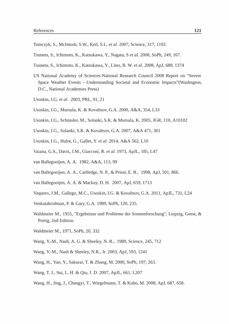
References 121
Tomczyk, S., McIntosh, S.W., Keil, S.L.et al.2007, Science, 317, 1192.
Tsuneta, S., Ichimoto, K., Katsukawa, Y., Nagata, Set al.2008, SoPh, 249, 167.
Tsuneta, S., Ichimoto, K., Katsukawa, Y., Lites, B. W.et al.2008, ApJ, 688, 1374
US National Academy of Sciences-National Research Council2008 Report on “Severe
Space Weather Events - Understanding Societal and EconomicImpacts”(Washngton,
D.C., National Academies Press)
Usoskin, I.G.et al. 2003, PRL, 91, 21
Usoskin, I.G., Mursula, K. & Kovaltsov, G.A. 2000, A&A, 354,L33
Usoskin, I.G., Schüssler, M., Solanki, S.K. & Mursula, K. 2005, JGR, 110, A10102
Usoskin, I.G., Solanki, S.K. & Kovaltsov, G.A. 2007, A&A 471, 301
Usoskin, I.G., Hulot, G., Gallet, Y.et al.2014, A&A 562, L10
Vaiana, G.S., Davis, J.M., Giacconi, R.et al.1973, ApJL, 185, L47
van Ballegooijen, A. A. 1982, A&A, 113, 99
van Ballegooijen, A. A., Cartledge, N. P., & Priest, E. R., 1998, ApJ, 501, 866.
van Ballegooijen, A. A. & Mackay, D. H. 2007, ApJ, 659, 1713
Vaquero, J.M., Gallego, M.C., Usoskin, I.G. & Kovaltsov, G.A. 2011, ApJL, 731, L24
Venkatakrishnan, P. & Gary, G.A. 1989, SoPh, 120, 235.
Waldmeier M., 1955, "Ergebnisse und Probleme der Sonnenforschung", Leipzig, Geest, &
Portig, 2nd Edition.
Waldmeier M., 1971, SoPh, 20, 332
Wang, Y.-M., Nash, A. G. & Sheeley, N. R., 1989, Science, 245,712
Wang, Y.-M., Nash & Sheeley, N.R., Jr. 2003, ApJ, 593, 1241
Wang, H., Yan, Y., Sakurai, T. & Zhang, M. 2000, SoPh, 197, 263.
Wang, T. J., Sui, L. H. & Qiu, J. D 2007, ApJL, 661, L207
Wang, H., Jing, J., Changyi, T., Wiegelmann, T. & Kubo, M. 2008, ApJ, 687, 658.
122 References
Wedemeyer-Böhm, S., Scullion, E., Steiner, O., van der Voort, L.R.et al.2012, Nature, 486,
505.
Weiss, N. 1981, JFM, 108, 247
Wilmot-Smith, A. L., Martens, P. C. H., Nandy, D., Priest, E.R., & Tobias, S. M. 2005,
MNRAS, 363, 1167
Wilmot-Smith, A. L., Nandy, D., Hornig, G., & Martens, P. C. H. 2006, ApJ, 652, 696
Withbroe, G.L. & Noyes, R.W. 1977, Annu. Rev. Astron. Astrophys., 15, 363.
Woltjer, L. 1958, PNAS, 44, 489
Yang, S.H., Zhang, J., Jin, C.L.et al. 2009, A&A, 501, 745
Yeates, A.R., Nandy, D. & Mackay, D.H. 2008, ApJ, 673, 544
Yokoyama, T., Akita, K., Morimoto, T., Inoue, K. & Newmark, J. 2001, ApJL, 546, L6
Yoshimura, H. 1975, ApJS, 29, 467
Yurchyshyn, V. B., Wang, H., Goode, P. R. & Deng, Y. 2001, ApJ,563, 381
Zhao, J., Bogart, R.S., Kosovichev, A.G., Duvall, Jr., T.L.& Hartlep, T. 2013, ApJL, 774,
L29
Zirker, J.B. 1993, SoPh, 148, 43.
20 22 24 26 28 30 32 34 36 38 40
−4
−3
−2
−1
0
1
2
3
4
Colatitude
Fie
ld S
tren
gth