IntroductionThe hierarchical latent OU model
Bayesian framework for statistical inferenceApplication of the OU model
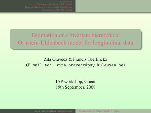
Estimation of a bivariate hierarchicalOrnstein-Uhlenbeck model for longitudinal data
Zita Oravecz & Francis Tuerlinckx(E-mail to: [email protected])
IAP workshop, Ghent19th September, 2008
[email protected] Estimation of a hierarchical OU model
IntroductionThe hierarchical latent OU model
Bayesian framework for statistical inferenceApplication of the OU model
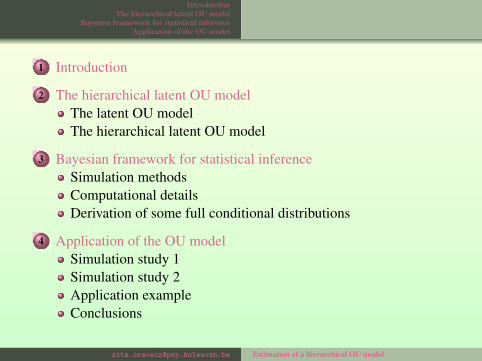
1 Introduction
2 The hierarchical latent OU modelThe latent OU modelThe hierarchical latent OU model
3 Bayesian framework for statistical inferenceSimulation methodsComputational detailsDerivation of some full conditional distributions
4 Application of the OU modelSimulation study 1Simulation study 2Application exampleConclusions
[email protected] Estimation of a hierarchical OU model

IntroductionThe hierarchical latent OU model
Bayesian framework for statistical inferenceApplication of the OU model
INTRODUCTION
[email protected] Estimation of a hierarchical OU model

IntroductionThe hierarchical latent OU model
Bayesian framework for statistical inferenceApplication of the OU model
Summary of the proposed model
Modeled data type: intensive longitudinal data (possiblyunstructured)
Observed data is a function of a latent continuous process
Bivariate SDE model for the changes in the latent true scorewithin the subject: an Ornstein-Uhlenbeck (OU) process
Hierarchically extended (multiple persons)
Time-varying and time-invariant covariate information can beincluded
Statistical inference: Bayesian framework
[email protected] Estimation of a hierarchical OU model

IntroductionThe hierarchical latent OU model
Bayesian framework for statistical inferenceApplication of the OU model
Typical area of applicability in psychology
Core affect measures
consciously accessible subjective aspect of feeling or emotion
compound of arousal (activation-deactivation) and hedonic(pleasantness-unpleasantness) values
when asked, people can report their CA
assumed to change continuously
[email protected] Estimation of a hierarchical OU model
IntroductionThe hierarchical latent OU model
Bayesian framework for statistical inferenceApplication of the OU model
The latent OU modelThe hierarchical latent OU model
THE HIERARCHICAL LATENT OUMODEL
[email protected] Estimation of a hierarchical OU model

IntroductionThe hierarchical latent OU model
Bayesian framework for statistical inferenceApplication of the OU model
The latent OU modelThe hierarchical latent OU model
Two-dimensional latent OU model
{dΘ(t) = B(µ−Θ(t))dt +σdW(t) (1)Y(t) = Θ(t)+ε(t) (2)
Eq. 1: transition equation: describes the change in the true score(dynamical aspect)
Eq. 2: observation equation: mapping of the true position on theobserved variable
dΘ(t): change in the variableB(µ−Θ(t))dt: deterministic partσdW(t): stochastic partinstantaneous covariance matrix: Σ = σσT
measurement error: ε(t)∼ N2(0,Σε)[email protected] Estimation of a hierarchical OU model
IntroductionThe hierarchical latent OU model
Bayesian framework for statistical inferenceApplication of the OU model
The latent OU modelThe hierarchical latent OU model
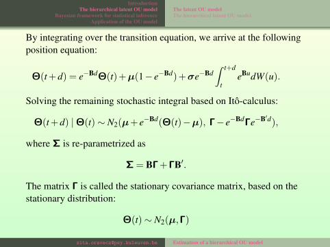
By integrating over the transition equation, we arrive at the followingposition equation:
Θ(t +d) = e−BdΘ(t)+µ(1− e−Bd)+σe−BdZ t+d
teBudW(u).
Solving the remaining stochastic integral based on Ito-calculus:
Θ(t +d) |Θ(t)∼ N2(µ+ e−Bd(Θ(t)−µ), Γ− e−BdΓe−B′d),
where Σ is re-parametrized as
Σ = BΓ+ΓB′.
The matrix Γ is called the stationary covariance matrix, based on thestationary distribution:
Θ(t)∼ N2(µ,Γ)
[email protected] Estimation of a hierarchical OU model

IntroductionThe hierarchical latent OU model
Bayesian framework for statistical inferenceApplication of the OU model
The latent OU modelThe hierarchical latent OU model
Hierarchical modeling
Individuals are random samples from a population
Each individual has person-specific OU parameters
AimsExplore general aspects of changes over timeExplain interindividual variability: regress random-effects ontocovariates
Notationp (p = 1, . . . ,P) is measured np times at: tp1, tp2, . . . , tps, . . . , tp,np .
Measured sequence of positions: Yp1, . . . ,Yps, . . . ,Yp,np
[email protected] Estimation of a hierarchical OU model

IntroductionThe hierarchical latent OU model
Bayesian framework for statistical inferenceApplication of the OU model
The latent OU modelThe hierarchical latent OU model
The hierarchical latent OU model
Yps = Θps +εps
εps ∼ N2(0,Σε)
Θps ∼ N2(Mps,Vps)
with
Mps ={
µps if s = 1µps + e−Bp(tps−tp,s−1)(Θp,s−1−µps) if s > 1
(1)
and covariance matrix
Vps ={
Γp if s = 1Γp− e−Bp(tps−tp,s−1)Γpe−B′p(tps−tp,s−1) if s > 1
(2)
[email protected] Estimation of a hierarchical OU model

IntroductionThe hierarchical latent OU model
Bayesian framework for statistical inferenceApplication of the OU model
The latent OU modelThe hierarchical latent OU model
Time-varying covariate information can be added through thehomebase parameter
µps = µp +(I2⊗ zps)δ
Time-varying effect on the homebase, e.g., the actual measurementtime
[email protected] Estimation of a hierarchical OU model

IntroductionThe hierarchical latent OU model
Bayesian framework for statistical inferenceApplication of the OU model
The latent OU modelThe hierarchical latent OU model
Decomposition of Bp and Γp
The positive definiteness has to be preserved:
Γp =
[γ1p
√γ1pγ2pργp√
γ1pγ2pργp γ2p
]
Bp =
[β1p
√β1pβ2pρβp√
β1pβ2pρβp β2p
]
[email protected] Estimation of a hierarchical OU model
IntroductionThe hierarchical latent OU model
Bayesian framework for statistical inferenceApplication of the OU model
The latent OU modelThe hierarchical latent OU model
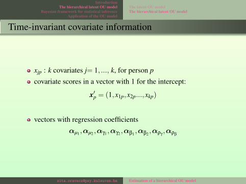
Time-invariant covariate information
xjp : k covariates j= 1, ..., k, for person p
covariate scores in a vector with 1 for the intercept:
x′p = (1,x1p,x2p...,xkp)
vectors with regression coefficients
αµ1 ,αµ2 ,αγ1 ,αγ2 ,αβ1 ,αβ2 ,αργ,αρβ
[email protected] Estimation of a hierarchical OU model

IntroductionThe hierarchical latent OU model
Bayesian framework for statistical inferenceApplication of the OU model
The latent OU modelThe hierarchical latent OU model
Population distributions
Homebase (target level) intercept (µp)
µp ∼ N2
( (x′pαµ1
x′pαµ2
),Σµ
)Volatility (Γp)
γ12p =√
γ1p×√
γ2p×ρp
γ1p ∼ LN(x′pαγ1 ,σ2γ1) γ2p ∼ LN(x′pαγ2 ,σ
2γ2)
Fisher-transformed cross-correlation
F(ργp) =12
log(
1+ργp
1−ργp
)∼ N(x′ργ
αργ,σ2
Fργ)
Centralizing tendency (Bp) follows the same decomposition as thevolatility
[email protected] Estimation of a hierarchical OU model

IntroductionThe hierarchical latent OU model
Bayesian framework for statistical inferenceApplication of the OU model
Simulation methodsComputational detailsDerivation of some full conditional distributions
BAYESIAN FRAMEWORK FORSTATISTICAL INFERENCE
[email protected] Estimation of a hierarchical OU model

IntroductionThe hierarchical latent OU model
Bayesian framework for statistical inferenceApplication of the OU model
Simulation methodsComputational detailsDerivation of some full conditional distributions
Bayesian statistical inference
Bayesian methods make explicit use of probability for quantifyinguncertainty
uncertainty rules of probability are used directly to makeinferences about the parameters
the inference is based on the actual occurring data (not allpossible data sets that might have occurred)
Bayesian parameter estimation: exploring the posterior density of theparameters
p(parameters|data) ∝ p(data|parameters)p(parameters)
[email protected] Estimation of a hierarchical OU model

IntroductionThe hierarchical latent OU model
Bayesian framework for statistical inferenceApplication of the OU model
Simulation methodsComputational detailsDerivation of some full conditional distributions
Simulation methods
Goal: generating samples from the posterior probability distribution
Direct simulation: prohibitively expensive (high-dimensionality)
Markov chain Monte Carlo simulation:
iterative sampling: drawing values from approximatedistributions, then correcting them
improved in each step: convergence to the target distribution
a sufficiently large number of iterations results in a Markov chainwith the posterior distribution as its equilibrium distribution
[email protected] Estimation of a hierarchical OU model
IntroductionThe hierarchical latent OU model
Bayesian framework for statistical inferenceApplication of the OU model
Simulation methodsComputational detailsDerivation of some full conditional distributions
Gibbs-sampler
Markov chain algorithm efficient for multidimensional problems
alternating conditional sampling: the parameter vector is dividedinto subparts
Full conditional distribution: the probability distribution of asubelement/subvector of the parameter vector, given the valuesof all other parameters as obtained in the previous iteration, aswell as the data
one iteration: the algorithm cycles through these subvectors,drawing each subset conditional on the other values
[email protected] Estimation of a hierarchical OU model

IntroductionThe hierarchical latent OU model
Bayesian framework for statistical inferenceApplication of the OU model
Simulation methodsComputational detailsDerivation of some full conditional distributions
Metropolis-Hastings (M-H) step
No known distributional form: a Metropolis-Hastings (M-H) step
adaptation of a random walk that uses acceptance/rejection ruleto converge to the target distribution
candidate is sampled from a proposal distribution
the decision of whether the new candidate is accepted is based onthe comparison of the density ratios (candidate vs. previouslyaccepted)
[email protected] Estimation of a hierarchical OU model

IntroductionThe hierarchical latent OU model
Bayesian framework for statistical inferenceApplication of the OU model
Simulation methodsComputational detailsDerivation of some full conditional distributions
Computational details
Sampling algorithm: custom-written MATLAB program
Subroutines of the program have been written in C (usingMATLAB’s MEX facility to interface)
Parallel computing can be applied (different sample chains areindependent and can be computed on separate processors)
Estimation of all model parameters by 15000 iterations in a 100subjects × 100 observations × 2 dimensions set-up on acomputing node with an AMD Opteron250 processor and 2Gb ofRAM takes approximately 5 hours
[email protected] Estimation of a hierarchical OU model

IntroductionThe hierarchical latent OU model
Bayesian framework for statistical inferenceApplication of the OU model
Simulation methodsComputational detailsDerivation of some full conditional distributions
DERIVATION OF SOME FULLCONDITIONAL DISTRIBUTIONS
[email protected] Estimation of a hierarchical OU model
IntroductionThe hierarchical latent OU model
Bayesian framework for statistical inferenceApplication of the OU model
Simulation methodsComputational detailsDerivation of some full conditional distributions
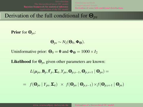
Derivation of the full conditional for Θps
Prior for Θps:
Θps ∼ N2(Θ0,ΦΘ).
Uninformative prior: Θ0 = 0 and ΦΘ = 1000× I2
Likelihood for Θps given other parameters are known:
L(µps,Bp,Γp,Σε,Yps,Θp,s−1,Θp,s+1 |Θps) =
= f (Θps | Yps,Σε) × f (Θps |Θp,s−1)× f (Θp,s+1 |Θps)
[email protected] Estimation of a hierarchical OU model

IntroductionThe hierarchical latent OU model
Bayesian framework for statistical inferenceApplication of the OU model
Simulation methodsComputational detailsDerivation of some full conditional distributions
Derivation of the full conditional for Θps
The values of the latent state Θps are drawn sequentially.
Full conditional for the Θps (except for s = np and s = 1 )
(Θps | µps,Bp,Γp,Σε,Yps,Θp,s−1,Θp,s+1) ∝
e− 1
2
{(Θps−Θ0
)TΦ−1
Θ
(Θps−Θ0
)}e− 1
2
{(Yps−Θps
)TΣ−1
εp
(Yps−Θps
)}e− 1
2
{(Θps−µps−e−BpdpsΘp,s−1+e−Bpdpsµps
)TV−1
ps
(Θps−µps−e−BpdpsΘp,s−1+e−Bpdpsµps
)}
e− 1
2
{(Θp,s+1−µp,s+1−e−Bpdp,s+1Θps+e−Bpdp,s+1µp,s+1
)TV−1
p,s+1(Θp,s+1−µp,s+1−e−Bpdp,s+1Θps+e−Bpdp,s+1µp,s+1
)}
which results in a normal distribution . . .
[email protected] Estimation of a hierarchical OU model

IntroductionThe hierarchical latent OU model
Bayesian framework for statistical inferenceApplication of the OU model
Simulation methodsComputational detailsDerivation of some full conditional distributions
(Θps | µps,Bp,Γp,Σε,Yps,Θp,s−1,Θp,s+1)∼ N2(MΘps ,VΘps)
where
VΘps = (Φ−1Θ
+Σ−1ε +V−1
ps +(e−Bpdp,s+1)TV−1p,s+1(e
−Bpdp,s+1))−1
and
MΘps = VΘps(Φ−1Θ
Θ0 +Σ−1εp
Yps +V−1ps µps +V−1
ps e−BpdpsΘp,s−1
−V−1ps e−Bpdpsµps +(e−Bpdp,s+1)TV−1
p,s+1Θp,s+1
−(e−Bpdp,s+1)TV−1p,s+1µp,s+1 +(e−Bpdp,s+1)TV−1
p,s+1e−Bpdp,s+1µp,s+1)
[email protected] Estimation of a hierarchical OU model

IntroductionThe hierarchical latent OU model
Bayesian framework for statistical inferenceApplication of the OU model
Simulation methodsComputational detailsDerivation of some full conditional distributions
Full conditional for Θp1
(Θp1 | µp1,Γp,Σε,Yp1)∼ N2(MΘp1 ,VΘp1)
with covariance matrix
VΘp1 = (Φ−1Θ
+Σ−1ε +Γ−1
p )−1
and mean
MΘp1 = VΘp1(Φ−1Θ
Θ0 +Σ−1ε Yp1 +Γ−1
p µp1)
[email protected] Estimation of a hierarchical OU model

IntroductionThe hierarchical latent OU model
Bayesian framework for statistical inferenceApplication of the OU model
Simulation methodsComputational detailsDerivation of some full conditional distributions
Full conditional for Θp,np
(Θp,np | µps,Bp,Γp,Σε,Yp,np)∼ N2(MΘp,np,VΘp,np
)
with covariance matrix
VΘp,np= (Φ−1
Θ+Σ−1
ε +V−1p,np
)−1
and mean
MΘp,np= VΘp,np
(Φ−1Θ
Θ0 +Σ−1εp
Yp,np +V−1p,np
µp,np+V−1
p,npe−Bpdp,np Θp,np−1
−V−1p,np
e−Bpdp,np µp,np).
[email protected] Estimation of a hierarchical OU model
IntroductionThe hierarchical latent OU model
Bayesian framework for statistical inferenceApplication of the OU model
Simulation methodsComputational detailsDerivation of some full conditional distributions
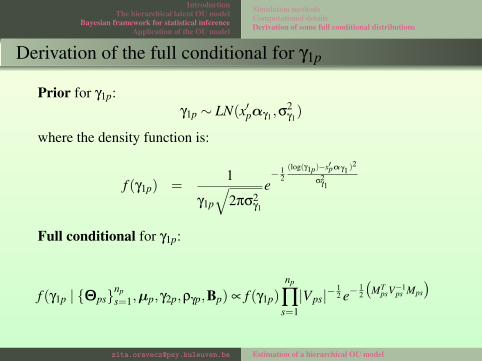
Derivation of the full conditional for γ1p
Prior for γ1p:γ1p ∼ LN(x′pαγ1 ,σ
2γ1)
where the density function is:
f (γ1p) =1
γ1p
√2πσ2
γ1
e− 1
2(log(γ1p)−x′pαγ1 )2
σ2γ1
Full conditional for γ1p:
f (γ1p | {Θps}nps=1,µp,γ2p,ργp,Bp) ∝ f (γ1p)
np
∏s=1|Vps|−
12 e−
12
(MT
psV−1ps Mps
)
[email protected] Estimation of a hierarchical OU model

IntroductionThe hierarchical latent OU model
Bayesian framework for statistical inferenceApplication of the OU model
Simulation study 1Simulation study 2Application exampleConclusions
APPLICATION OF THE OUMODEL
[email protected] Estimation of a hierarchical OU model

IntroductionThe hierarchical latent OU model
Bayesian framework for statistical inferenceApplication of the OU model
Simulation study 1Simulation study 2Application exampleConclusions
Study 1
Ten data sets were simulated based on the results of a real lifeapplication
ten measurements per day, for ten days, for 100 subjects
semi-random measurement time-points
two longitudinal variables
measurement time-points were used as linear and quadratictime-effects
Estimationfor each dataset 3 chains were run15 000 iterations per chain5 000 discarded burn-incomputation time: 5 hours per chain
[email protected] Estimation of a hierarchical OU model

IntroductionThe hierarchical latent OU model
Bayesian framework for statistical inferenceApplication of the OU model
Simulation study 1Simulation study 2Application exampleConclusions
Model Simulated Mean posterior SD of the posteriorParameter value estimate estimates
αµ1 6.00 5.99 0.04αµ2 5.00 4.97 0.07σ2
µ10.40 0.42 0.07
σµ1µ2 0.05 0.04 0.04σ2
µ20.30 0.27 0.05
δLµ1 1.00 1.00 0.12δQµ1 0.00 -0.01 0.12δLµ2 4.00 3.96 0.12δQµ2 -4.00 -4.00 0.14αγ1 0.80 0.77 0.07σ2
γ10.40 0.38 0.04
αγ2 1.00 1.01 0.10σ2
γ20.20 0.20 0.03
αγρ 0.10 0.09 0.03σ2
γρ0.10 0.08 0.01
αβ1-4.20 -4.21 0.04
σ2β1
0.40 0.39 0.10
αβ2-4.00 -3.93 0.09
σ2β2
0.50 0.49 0.18
αβρ-0.10 -0.11 0.03
σ2βρ
0.10 0.08 0.02
σ21ε
0.20 0.21 0.04σ2
2ε1.00 0.88 0.13
[email protected] Estimation of a hierarchical OU model

IntroductionThe hierarchical latent OU model
Bayesian framework for statistical inferenceApplication of the OU model
Simulation study 1Simulation study 2Application exampleConclusions
Posterior density estimates
[email protected] Estimation of a hierarchical OU model

IntroductionThe hierarchical latent OU model
Bayesian framework for statistical inferenceApplication of the OU model
Simulation study 1Simulation study 2Application exampleConclusions
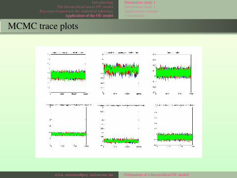
MCMC trace plots
[email protected] Estimation of a hierarchical OU model
IntroductionThe hierarchical latent OU model
Bayesian framework for statistical inferenceApplication of the OU model
Simulation study 1Simulation study 2Application exampleConclusions
MCMC trace plots
[email protected] Estimation of a hierarchical OU model

IntroductionThe hierarchical latent OU model
Bayesian framework for statistical inferenceApplication of the OU model
Simulation study 1Simulation study 2Application exampleConclusions
MCMC trace plots
[email protected] Estimation of a hierarchical OU model

IntroductionThe hierarchical latent OU model
Bayesian framework for statistical inferenceApplication of the OU model
Simulation study 1Simulation study 2Application exampleConclusions
Study 2
Ten data sets were simulated based on a more arbitrary design
the levels of measurement error were increased
in the first dimension: higher measurement error (σ21ε
= 4) thanstochastic variance (αγ1 = 1, expected value appr.: 3.5)
cross-effects were substantial (σ2γρ
= 0.5 and αβρ= 0.5)
[email protected] Estimation of a hierarchical OU model

IntroductionThe hierarchical latent OU model
Bayesian framework for statistical inferenceApplication of the OU model
Simulation study 1Simulation study 2Application exampleConclusions
Model Simulated Mean posterior SD of the posteriorParameter value estimate estimates
αµ1 0.00 -0.04 0.12αµ2 0.00 -0.01 0.14σ2
µ12.00 2.14 0.32
σµ1µ2 0.70 0.71 0.23σ2
µ21.00 0.93 0.17
δLµ1 2.00 1.86 0.22δQµ1 0.00 0.10 0.22δLµ2 0.00 -0.01 0.26δQµ2 4.00 3.99 0.26αγ1 1.00 1.32 0.11σ2
γ10.50 0.28 0.05
αγ2 2.00 1.95 0.10σ2
γ20.10 0.10 0.02
αγρ 0.50 0.41 0.05σ2
γρ0.10 0.05 0.01
αβ1-4.00 -3.75 0.24
σ2β1
0.50 0.40 0.26
αβ2-3.50 -3.44 0.20
σ2β2
0.10 0.18 0.13
αβρ0.50 0.38 0.07
σ2βρ
0.10 0.06 0.03
σ21ε
4.00 3.20 0.24σ2
2ε2.00 2.13 0.73
[email protected] Estimation of a hierarchical OU model
IntroductionThe hierarchical latent OU model
Bayesian framework for statistical inferenceApplication of the OU model
Simulation study 1Simulation study 2Application exampleConclusions
APPLICATION EXAMPLE
[email protected] Estimation of a hierarchical OU model

IntroductionThe hierarchical latent OU model
Bayesian framework for statistical inferenceApplication of the OU model
Simulation study 1Simulation study 2Application exampleConclusions
Data collection
Participants: 80 students from the University of Leuven
Method:Experience sampling
wristwatch
beeps 9 times perday for 7 days
semi-random beeps
Core Affect Grid −→
Descriptivesaverage 60 (SD=3.4) measurements (missingness: MAR)age 21 (SD=4.7)60% women
[email protected] Estimation of a hierarchical OU model
IntroductionThe hierarchical latent OU model
Bayesian framework for statistical inferenceApplication of the OU model
Simulation study 1Simulation study 2Application exampleConclusions
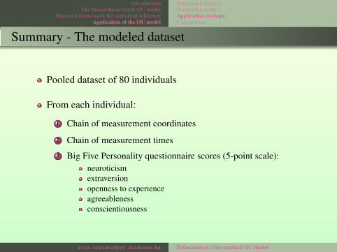
Summary - The modeled dataset
Pooled dataset of 80 individuals
From each individual:
1 Chain of measurement coordinates
2 Chain of measurement times
3 Big Five Personality questionnaire scores (5-point scale):neuroticismextraversionopenness to experienceagreeablenessconscientiousness
[email protected] Estimation of a hierarchical OU model

IntroductionThe hierarchical latent OU model
Bayesian framework for statistical inferenceApplication of the OU model
Simulation study 1Simulation study 2Application exampleConclusions
Details of the Bayesian inference
non-informative priors were assigned
posterior estimates are based on 10000 iterations with 6 chains
burn-in: 5000 iterations
computation time: fewer than 2 hours per chain
convergence checked (R statistics, visual assessment)
[email protected] Estimation of a hierarchical OU model
IntroductionThe hierarchical latent OU model
Bayesian framework for statistical inferenceApplication of the OU model
Simulation study 1Simulation study 2Application exampleConclusions
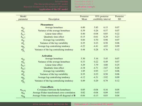
Model Posterior 95% posterior Posteriorparameter Description Mean credibility interval SD
Pleasantnessαµ1 Average homebase 6.00 5.85 6.15 0.07σ2
µ1Variance of the average homebase 0.39 0.26 0.57 0.07
δµ11 Linear time-effect 0.40 -0.04 0.85 0.22δµ12 Quadratic time-effect -0.15 -0.61 0.29 0.23αγ1 Average log-variability 0.84 0.70 0.98 0.07σ2
γ1Variance of the log-variability 0.35 0.23 0.50 0.06
αβ1Average log-centralizing tendency -4.22 -4.41 4.03 0.09
σ2β1
Variance of the log-centralizing tendency 0.48 0.28 0.76 0.12
Activationαµ2 Average homebase 5.30 5.16 5.45 0.07σ2
µ2Variance of the average homebase 0.33 0.22 0.49 0.07
δµ21 Linear time-effect 4.29 3.79 4.80 0.25δµ22 Quadratic time-effect -4.18 -4.71 -3.67 0.26αγ2 Average log-variability 1.05 0.93 1.17 0.06σ2
γ2Variance of the log-variability 0.35 0.23 0.50 0.06
αβ2Average log-centralizing tendency -4.12 -4.31 -3.92 0.09
σ2β2
Variance of the log-centralizing tendency 0.49 0.29 0.79 0.12
Cross-effectsσµ1µ2 Covariance between the homebases 0.05 -0.04 0.16 0.05αργ Average Fisher transformed cross-correlation 0.02 -0.04 0.09 0.03αρ
βAverage Fisher transformed off-diagonal of B -0.04 -0.13 0.03 0.04
[email protected] Estimation of a hierarchical OU model

IntroductionThe hierarchical latent OU model
Bayesian framework for statistical inferenceApplication of the OU model
Simulation study 1Simulation study 2Application exampleConclusions
Time-varying effect estimates
[email protected] Estimation of a hierarchical OU model

IntroductionThe hierarchical latent OU model
Bayesian framework for statistical inferenceApplication of the OU model
Simulation study 1Simulation study 2Application exampleConclusions
Person-specific autocorrelation estimates
[email protected] Estimation of a hierarchical OU model

IntroductionThe hierarchical latent OU model
Bayesian framework for statistical inferenceApplication of the OU model
Simulation study 1Simulation study 2Application exampleConclusions
Model Posterior 95% Posterior Posteriorparameter Description Covariate mean credibility interval SD
Pleasantnessαµ1N Homebase Neuroticism -0.32 -0.58 -0.07 0.13α
γ1N Variability Neuroticism 0.26 0.01 0.51 0.12Cross-effects
αργN Cross-correlation Neuroticism 0.13 0.01 0.25 0.06
αργC Cross-correlation Conscientiousness -0.18 -0.30 -0.05 0.06
αρ
βA Off-diagonal of B Agreeableness -0.25 -0.45 -0.07 0.09
Note. Model parameters refer to the regression weights. For example αµ1N is the regression weight for neuroticism relating tothe homebase in the pleasantness dimension (µ1).
[email protected] Estimation of a hierarchical OU model
IntroductionThe hierarchical latent OU model
Bayesian framework for statistical inferenceApplication of the OU model
Simulation study 1Simulation study 2Application exampleConclusions
CONCLUSIONS
[email protected] Estimation of a hierarchical OU model

IntroductionThe hierarchical latent OU model
Bayesian framework for statistical inferenceApplication of the OU model
Simulation study 1Simulation study 2Application exampleConclusions
Conclusions
Recovery was sufficient, better for the simulation with smallermeasurement error (less noisy measurements )
Bayesian methodology can be efficiently applied to estimateSDE models with known probability density function of thestates
Extension to more dimensions is possible
Model testing can be done in the Bayesian framework, e.g., DIC
[email protected] Estimation of a hierarchical OU model

IntroductionThe hierarchical latent OU model
Bayesian framework for statistical inferenceApplication of the OU model
Simulation study 1Simulation study 2Application exampleConclusions
THANK YOUFOR YOUR ATTENTION!
[email protected] Estimation of a hierarchical OU model