Estimating inflation risk premia from nominal and real yield curves using a shadow-rate model Kei Imakubo* [email protected] Jouchi Nakajima** [email protected]
No.15-E-1 April 2015
Bank of Japan 2-1-1 Nihonbashi-Hongokucho, Chuo-ku, Tokyo 103-0021, Japan
* Monetary Affairs Department ** Monetary Affairs Department
Papers in the Bank of Japan Working Paper Series are circulated in order to stimulate discussion and comments. Views expressed are those of authors and do not necessarily reflect those of the Bank. If you have any comment or question on the working paper series, please contact each author.
When making a copy or reproduction of the content for commercial purposes, please contact the Public Relations Department ([email protected]) at the Bank in advance to request permission. When making a copy or reproduction, the source, Bank of Japan Working Paper Series, should explicitly be credited.
Bank of Japan Working Paper Series
1
Estimating inflation risk premia from nominal and real
yield curves using a shadow‐rate model
Kei Imakubo† and Jouchi Nakajima‡
April 2015
Abstract
This paper proposes and estimates an extended shadow-rate term structure model, and uses it to extract inflation risk premia from nominal and real term structures. Our model incorporates the shadow rate and thereby explicitly takes account of the zero lower bound constraint of nominal interest rates. The estimation results for Japan and the United States confirm that our model successfully avoids the estimation bias inherent in the standard affine-type term structure model that ignores the zero lower bound. As we theoretically and empirically demonstrate, the inflation risk premium is time-varying and takes both positive and negative values reflecting market concerns with regard to asymmetric uncertainty in future inflation.
JEL classification: E31, E43, E52, G12
Keywords: Arbitrage-free term structure; Inflation risk premium; Shadow rate; Term premium; Zero lower bound
We are grateful for the helpful comments from the staff of the Bank of Japan. The views expressed herein are those of the authors alone and do not necessarily reflect those of the Bank of Japan. † Monetary Affairs Department, Bank of Japan ([email protected]) ‡ Monetary Affairs Department, Bank of Japan ([email protected])

2
1. Introduction
The affine-type term structure (ATS) model introduced by Duffie and Kan (1996) has
become a widely accepted approach to decomposing nominal yields into the expected
future path of short-term interest rates and the term premia (see Duffie, 2001, for an
overview of arbitrage-free term structure models). The standard ATS model specifies the
latent factors driving the economy based on vector autoregression, and assumes that
instantaneous interest rates and the market prices of risk are affine in those factors. The
specification leads to an observation equation where log yields are affine in those
factors. The resulting linear state space form is computationally tractable under
arbitrage-free conditions and allows estimation by the Kalman filter and maximum
likelihood method with the additional assumption of Gaussian errors for the observation
and state equations. This model has led to a wide range of applications and extensions in
the literature.1
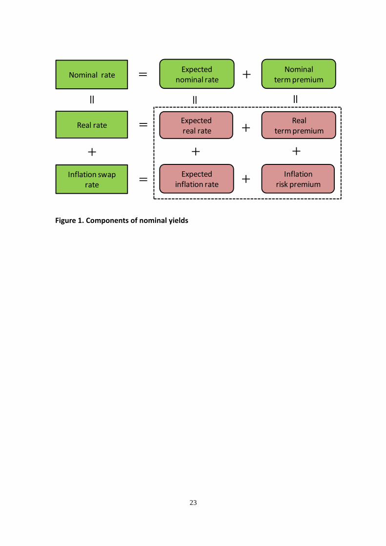
As illustrated in Figure 1, a nominal bond yield can be decomposed into four
components: expected real rate, real term premium, expected inflation, and inflation risk
premium. This decomposition has become an accepted practice for measuring the
effects of monetary policy. Using the estimation results of the standard ATS model by
D'Amico et al. (2010), Bernanke (2013a) discusses the background of the decline in U.S.
long-term bond yields. Christensen et al. (2010) and Joyce et al. (2010) decompose U.S.
and U.K. bond yields, respectively, and address the dynamics of the expected inflation
and the inflation risk premium.2 Note that major central banks have implemented
unconventional policy measures recently. Bauer and Rudebusch (2014) and Joyce et al.
(2011) measure the effects of U.S. and U.K. central banks' asset purchases on the bond
yield term premium. The interest-rate formation under unconventional monetary policy
will attract further attention.
It is well known that the standard ATS model does not rule out negative rates of
1 See, for example, Dai and Singleton (2000), Kim and Wright (2005), and Adrian et al. (2013). 2 See also Ang et al. (2008), Adrian and Wu (2009), and Chernov and Mueller (2012) for an analysis of U.S. bond yields; García and Werner (2010), and Hördahl and Tristani (2010, 2012) for euro-area bond yields.
3
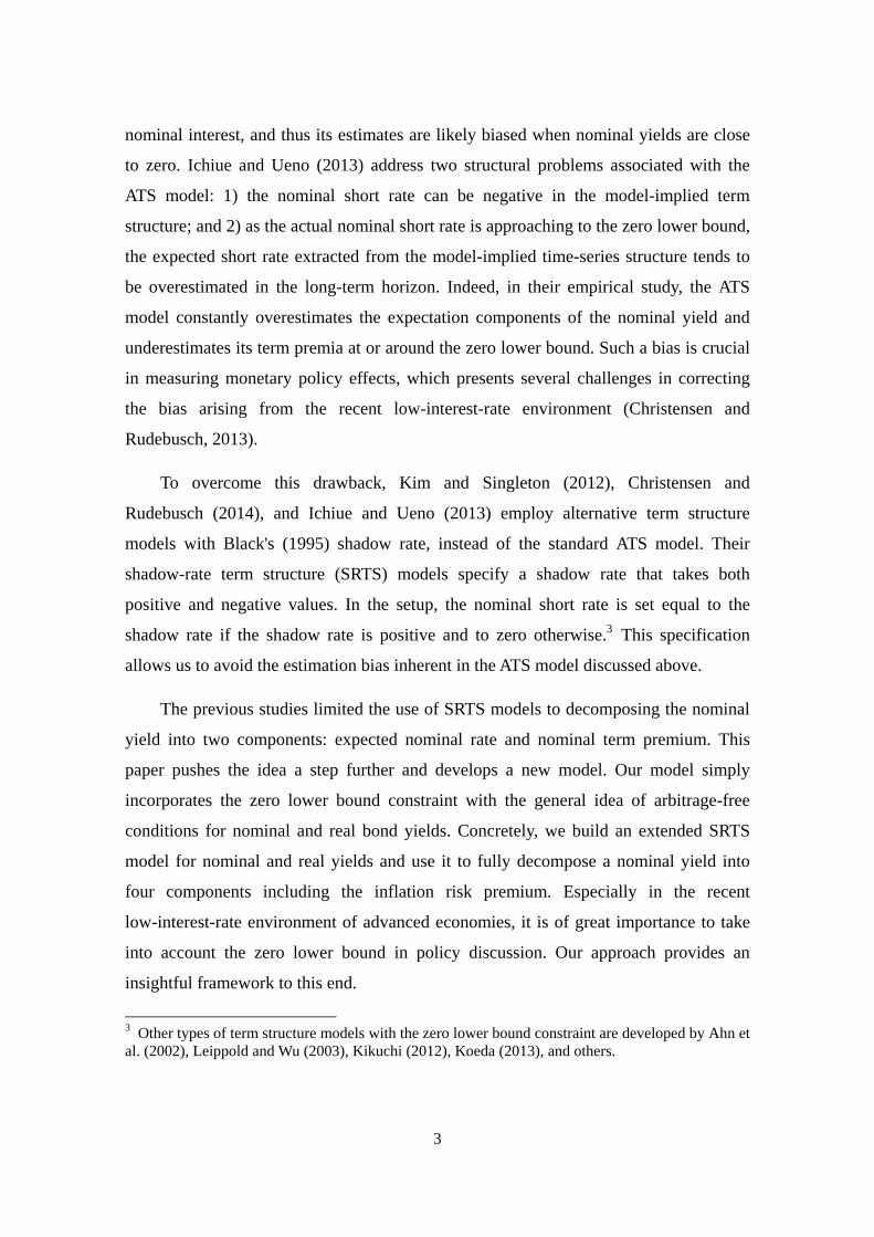
nominal interest, and thus its estimates are likely biased when nominal yields are close
to zero. Ichiue and Ueno (2013) address two structural problems associated with the
ATS model: 1) the nominal short rate can be negative in the model-implied term
structure; and 2) as the actual nominal short rate is approaching to the zero lower bound,
the expected short rate extracted from the model-implied time-series structure tends to
be overestimated in the long-term horizon. Indeed, in their empirical study, the ATS
model constantly overestimates the expectation components of the nominal yield and
underestimates its term premia at or around the zero lower bound. Such a bias is crucial
in measuring monetary policy effects, which presents several challenges in correcting
the bias arising from the recent low-interest-rate environment (Christensen and
Rudebusch, 2013).
To overcome this drawback, Kim and Singleton (2012), Christensen and
Rudebusch (2014), and Ichiue and Ueno (2013) employ alternative term structure
models with Black's (1995) shadow rate, instead of the standard ATS model. Their
shadow-rate term structure (SRTS) models specify a shadow rate that takes both
positive and negative values. In the setup, the nominal short rate is set equal to the
shadow rate if the shadow rate is positive and to zero otherwise.3 This specification
allows us to avoid the estimation bias inherent in the ATS model discussed above.
The previous studies limited the use of SRTS models to decomposing the nominal
yield into two components: expected nominal rate and nominal term premium. This
paper pushes the idea a step further and develops a new model. Our model simply
incorporates the zero lower bound constraint with the general idea of arbitrage-free
conditions for nominal and real bond yields. Concretely, we build an extended SRTS
model for nominal and real yields and use it to fully decompose a nominal yield into
four components including the inflation risk premium. Especially in the recent
low-interest-rate environment of advanced economies, it is of great importance to take
into account the zero lower bound in policy discussion. Our approach provides an
insightful framework to this end.
3 Other types of term structure models with the zero lower bound constraint are developed by Ahn et al. (2002), Leippold and Wu (2003), Kikuchi (2012), Koeda (2013), and others.

4
This paper is structured as follows. Section 2 describes the newly developed SRTS
model for nominal and real yields and illustrates the method of estimation. Section 3
applies the model to Japan's and U.S. yields. Section 4 concludes.
2. Shadow‐rate term structure model
This section describes the extended SRTS model for nominal and real yields and
explains its estimation method. Our approach does not rely on any structural
assumptions about the macro economy, as the macro-finance approaches do. Instead,
our approach adopts only the arbitrage-free assumption. Using only a few latent factors,
the model captures the characteristics of the term structure and dynamics of nominal
and real yields. Moreover, the combination of the shadow rate and zero lower bound
enables us to reasonably describe the flattening of the nominal yield curve as it gets
closer to zero percent.
2.1 Model structure
Shadow rate
Define as the 1) vector of latent factors governing the term structure and
dynamics of bond yields. Let denote the instantaneous shadow rate, which is
defined as an affine function of the factors. Then, the nominal instantaneous short rate,
denoted by , is defined as follows:
max , ,
where
.
In the above, is the lower bound of the nominal short rate.4 The model can avoid a
negative nominal short rate in the following fashion: when is above , is
equal to ; when is below , is equal to . The standard ATS model
4 When a central bank pays interest on excess reserves, we assign a slightly positive value to according to the level of interest rates on excess reserves. Unless otherwise mentioned, we set equal to zero (see Ichiue and Ueno, 2013).

5
directly specifies the nominal short rate as an affine function of the factors,
, and does not rule out negative values of .
We model the real instantaneous short rate as an affine function of the factors. The
real short rate takes both positive and negative values and is free from the zero lower
bound. Let denote the real short rate, which is given by
.
Dynamics of the factors, which are common to nominal and real short rates, are
specified as the following Gaussian process under the objective -measure:
Σ ,
where is a standard -dimension Brownian motion under the -measure.
Stochastic discount factors and market prices of risk
With the stochastic discount factor , , , where stands for "nominal"
and for "real," the bond price , and the zero-coupon yield , of -year
maturity at time are given by
, E , , , and
, log , log E , , .
We assume the following process of the stochastic discount factor:
, , ,
where is the ( 1) vector of the market prices of risk, specified by the affine
function of the factors:
Λ , , .
Given these settings, the arbitrage-free condition implies

6
, log E exp , , , (1)
where E · denotes the conditional expectation under the risk-neutral -measure.
Here we define the expected nominal/real rates, denoted by ,, E , as
the average of the expected nominal/real short rates from time to . Also, we
define the nominal/real term premium, denoted by ,,TP, as the difference between the
zero-coupon yield and the expected nominal/real rate. This means that the zero-coupon
yield is decomposed as
, ,, ,
,TP , , .
Real and inflation components
We define the inflation components as the difference between the nominal and
real yields. Let denote the level of general prices, i.e., 1 , where is
the inflation rate. Following Christensen et al. (2010), the arbitrage-free condition
implies that is equal to the ratio of the real and nominal stochastic discount factors,
i.e., / . This leads to the following decomposition of the nominal bond price
, .
, E E /
/
E E Cov ,
E E 1 C ,
E E.
In terms of yield components, we have
, , , ,RP
,, ,
,TP , ,RP, (2)
where , is the expected inflation and ,RP is the inflation risk premium, that is,
7
, log E , and
,RP log 1
C ,
E E. (3)
As shown in Equation (2), the nominal yield consists of four components: expected real
rate, real term premium, expected inflation, and inflation risk premium.
Interpretation of inflation risk premia
The inflation risk premium is compensation for real return uncertainty caused by
unexpected inflation/deflation. The model-implied inflation risk premium in Equation
(3) can take both positive and negative values, depending on the correlation between the
real stochastic discount factor and inflation expectations. The inflation risk premium is
positive (negative) when / and / are negatively (positively) correlated.
The real stochastic discount factor, or the pricing kernel, can be interpreted in
several ways. One standard interpretation in the literature is that the real stochastic
discount factor corresponds to the investors' marginal rate of substitution as shown in
the capital asset pricing model (CAPM). As discussed by Campbell et al. (2009), the
covariance in Equation (3) can be reinterpreted as the covariance between the
representative agents' intertemporal rate of marginal substitution and their inflation
expectations. For example, if inflation rises unexpectedly when the marginal utility is
high, the real return for holding nominal bonds falls unexpectedly. In this case, the
nominal bonds are risky assets and bond investors charge a positive premium on the
bonds. Conversely, if inflation falls unexpectedly when the marginal utility is high, the
investors benefit from holding the nominal bonds. Then, they are willing to pay a
premium on the bonds. In this case, the inflation risk premium is negative.5
Another interpretation of the positive/negative signs of the inflation risk premium
is derived from the nature of inflation derivatives. A long position of inflation swaps can
5 The opposite holds when the marginal utility is low. For example, the model-implied correlation in the case of a positive inflation risk premium implies that inflation tends to be lower than expected.

8
be replicated by a synthetic position of call and put options with the inflation rate as an
underlying asset. Buying an inflation call with a strike price of , while selling an
inflation put with the same strike price generates an inflation swap payoff. Obviously
the sign of the inflation risk premium depends on which is greater, the call premium or
the put premium.
Consider how to price inflation call and put options that pay off inflation-linked
floating rates at the terminal in the absence of arbitrage opportunities:
E · max , , 0 ,
E · max , , 0 ,
where and are European call and put premia, respectively, and is an
appropriate stochastic discount factor. Using these two prices, the price of the synthetic
position of a long call and a short put is given by
E · ,
E E , . (4)
From the covariance term in Equation (3), we have
Cov , E E E
E E ,exp. (5)
In the last equality, we assumed that is homogeneous in / . We note that
Equation (5) derived from our SRTS model corresponds to Equation (4) derived from a
simple asset pricing framework. This interpretation, which assumes only an
arbitrage-free condition and requires neither representative agents nor complete markets,
holds in almost any environment in which inflation swaps are traded. For example,
when Equation (5) is positive, the inflation call premium is larger than the inflation put
premium. In this case, investors are more concerned with an inflation rate that is
unexpectedly higher than the expected inflation , and therefore pay a positive
premium on the inflation risk. On the contrary, when Equation (5) is negative, the call
9
premium is less than the put premium, meaning that the inflation risk premium is below
zero. Such a negative premium on inflation risks suggests that investors are more
concerned with unexpectedly lower inflation or deflation.
2.2 Estimation method
In this paper, we set the number of factors to 4. Specifically, the dynamics of the
nominal yield curve are governed by two latent factors, while those of the real yield
curve are governed by those two factors and two additional factors that are specific to
the real yields. To make the model parsimonious, we restrict the parameters as follows:
1, 1, 0, 0 , , , 1, 1 ,
, , 0, 0 , , , , ,
ΛΛ
, ΛΛ ΛΛ Λ ,
Σ diag , … , ,
where Λ is a (2 2) matrix ( , 1, 2), and diag · denotes a diagonal matrix.
The SRTS model can be estimated in the form of a state space model consisting of
observation equations and state equations. To derive the form, we rewrite the nominal
yield in Equation (1) as follows:6
, E . (6)
The zero lower bound constraint on the nominal yield makes it impossible to derive any
analytical solution due to the existence of the integral in Equation (6). As suggested by
Ichiue and Ueno (2013), we conditionally linearize the right-hand side of Equation (6)
around the one-month-ahead linear-least-square forecast of the factors made in the
previous month. We let , denote the linearly approximated function of the
6 From Equation (1), for , we have log E exp E , ,
where , is the Jensen term. Ichiue and Ueno (2013) report that the Jensen term of the 10-year nominal yield is about 5 basis points and smaller than the estimated nominal term premium in their empirical study. They conclude that it does not matter if they ignore the Jensen term in their estimation. The current paper also sets , 0 to reduce computational burdens.

10
right-hand side of Equation (6).
The real yield is free from the zero lower bound constraint. As in Duffie and Kan
(1996), the observation equation of the real yield in Equation (1) is given in the form of
an affine function:
, ,
where and are the functions of the model parameters and the maturity .
To sum up, we estimate the state space model below.
Observation equation: , ~ 0, ,
State equation: Φ Γ , ~ 0, ,
with
, ,
where and are vectors of the observed yields of maturities , … , ;
, , … , , , for , ; and are vectors, the -th column of which
is , and , respectively, for 1,… , ; Φ and Γ are
matrices of functions of the model parameters; and is a diagonal matrix. The
observation equation of the nominal yield is nonlinear with respect to the factors. For
nonlinear estimation, we employ the extended Kalman filter method to obtain the
maximum likelihood estimate.
3. Empirical analysis
3.1 Data
This section applies our SRTS model to Japan's and U.S. yield data. The data are
monthly series (end-of-month) of nominal and real zero-coupon rates from January
1995 to December 2014. The real zero-coupon rate is given as the difference in the
nominal zero-coupon rate from the zero-coupon inflation swap rate.7,8
7 We compute Japan's zero-coupon rate using the method of McCulloch (1990), and use U.S. zero-coupon rate, available on the website of the Federal Reserve: www.federalreserve.gov/pubs/ feds/2006/200628/200628abs.html, which is computed using the method of Gürkaynak et al. (2007).

11
In the literature, a series of inflation-indexed bond rates is often used as the real
zero-coupon rate to estimate term structure models. 9 However, as discussed by
D'Amico et al. (2010) and others, the size of the liquidity premium on inflation-indexed
bonds cannot be ignored. Inflation-indexed bonds, whose markets have only a short
history compared with fixed-coupon bond markets, are not sufficiently liquid to sell and
buy in a timely manner.10 Especially in Japan, new issuance of Japanese government
inflation-indexed bonds (JGBi) was halted for several years after the Lehman shock,
resulting in insufficient data to compute a zero-coupon yield curve. Inflation swaps have
a much shorter history and are traded by a limited number of market participants.
Nevertheless, inflation swaps, over-the-counter derivatives, have the following
advantages. First, they are essentially free from the direct effects of supply-demand
conditions for cash bonds and of funding. Second, we can observe stable and continuous
rate dynamics backed by market makers who keep quoting offer and bid prices.11
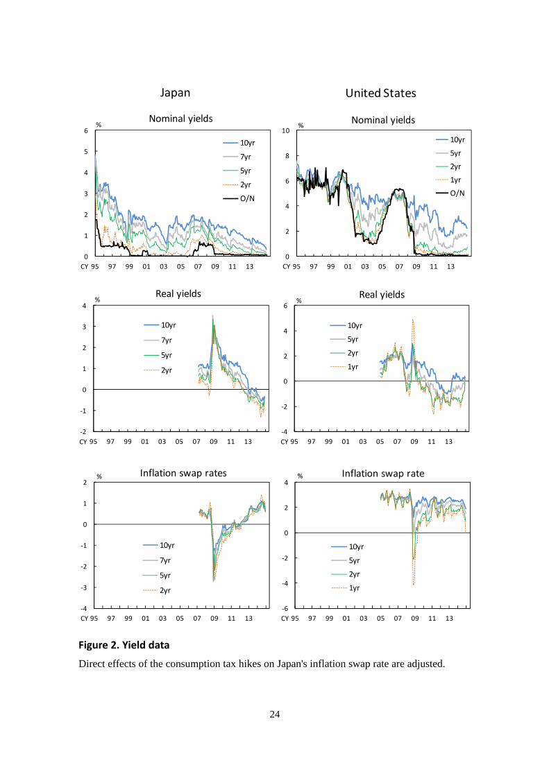
The analysis uses overnight rates and zero-coupon rates for the selected terms to
maturity. The overnight rates are used as the nominal short rate: the uncollateralized
overnight call rate for Japan and the overnight federal funds rate for the United States.12
As the terms to maturity of the zero-coupon rates, we select 2, 5, 7, and 10 years for
Japan, and 1, 2, 5, and 10 years for the United States. Importantly, we note that the
nominal yield curve of Japanese government bonds (JGB) in our sample period has a
flattening shape with a short horizon and a kinked shape around the term of 7 years,
which, in a low-interest-rate environment, corresponds to the term of the current
8 For Japan's inflation swap rate, the direct effects of the actual and planned consumption tax hikes (one from 5 percent to 8, and the other from 8 to 10) on the swap rate are adjusted prior to the analysis. Specifically, we mechanically calculate the theoretical effects of the tax hikes on the yield curve of the break-even inflation under the assumption that the tax hikes will be fully passed on to all current taxable items. We then regress those tax effects on the observed yield curve of inflation swaps to measure the probability of the tax hikes that the market takes into consideration in pricing the break-even inflation rate, and obtain the adjusted yield excluding the effects of the tax hikes. 9 The method developed by Gürkaynak et al. (2010) is commonly used. 10 The first U.S. Treasury inflation-protected securities (TIPS) were issued in January 1997. Japanese government inflation-indexed bonds (JGBi) were first issued in March 2004 and temporarily stopped from August 2008 to September 2013. 11 Haubrich et al. (2012) use inflation swap rates to estimate the ATS model for nominal and real yields. 12 As for Japan, until March 1995, the official discount rate is used as the nominal short rate.

12
cheapest-to-deliver bonds that settle JGB futures contracts. Against this background, we
drop the 1-year yield from the candidate terms because of the insignificant difference in
information between 1-year and 2-year yields,13 and adopt the 7-year yield to capture
the yield dynamics around that term. The yield data are plotted in Figure 2.14
In this analysis, the real yields are only available from April 2007 for Japan, and
from January 2005 for the United States, due to data availability of inflation swap rates.
Therefore, the yield is set as , when the real yields are not available at
1,… , ; and , when both the nominal and real yields are available at
1,… , where and are vectors of the nominal and real yields,
respectively. With regard to this data structure, we note two technical issues in the
estimation. First, we adjust the dimensions of the variables in the extended Kalman
filter according to the number of observation equations, which changes depending on
the period. Second, we include an additional observation equation to complement the
yield information, which indicates the model-implied convergence point of the expected
inflation, in order to make the estimation more robust. Specifically, we adopt the survey
on 10-year expected inflation from the Consensus Forecasts as a dependent variable,
and the difference in the model-implied extremely long (50-year) expected nominal rate
from the expected real rate as an independent variable.15,16 This equation is included in
the model for the periods when the real yields are available.
13 In the estimation of Japan's yields, estimation errors in short-horizon yields tend to be larger when the term to maturity is 1 year. For this reason, we set an additional observation equation referring to the slope of the yield curve in the short horizon instead of the observation equation for the 1-year yield. Specifically, the additional equation is given by the 1-year ahead 2-year forward overnight-indexed swap rate as a dependent variable and the model-implied corresponding expected nominal forward rate as an independent variable. 14 Real yields and inflation swap rates in the crisis period just after the Lehman shock exhibit a spike. In this period, there was a significant unwinding of convergence trading positions around the globe, which brought a sharp drop in market liquidity through a reduction in brokers' market-making ability (Bank of Japan, 2009). 15 Guimarães (2014) shows that robust estimates are obtained by adding survey information to the observation equation of the ATS model. Such reference information is incorporated in D'Amico et al. (2010), Joyce et al. (2010) and others. Instead of the expected inflation in our analysis, a nominal extremely-long forward rate might be an alternative reference. 16 From the Consensus Forecasts data obtained from Consensus Economics Inc., we use biannual series, which are linearly interpolated to obtain a smoothed monthly series for the estimation.
13
3.2 Estimation results
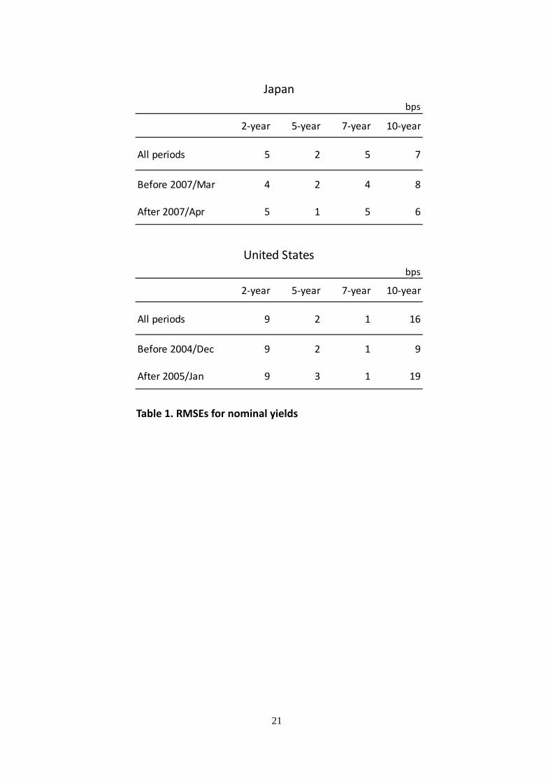
Table 1 reports the root mean squared error (RMSE) for each term of maturity. It shows
that the maximum RMSE for all periods is only 7 basis points for Japan and 16 basis
points for the Unites States. The RMSEs for two sub-periods are also reported. The first
period (before March 2007 for Japan and before December 2004 for the United States)
uses only the nominal yields to estimate the model and the second period (after April
2007 for Japan and after January 2005 for the United States) uses both the nominal and
real yields. As mentioned above, we change the number of observation equations
depending on the period. The table shows that the RMSEs are reasonably small for both
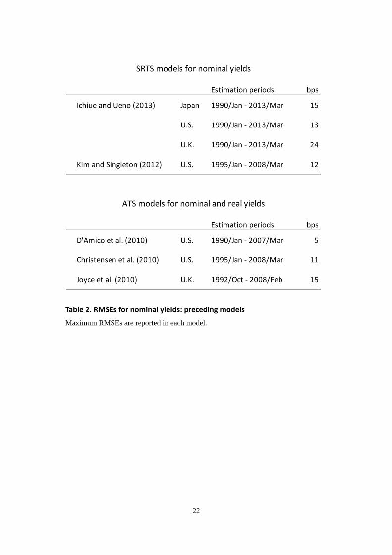
periods. This result is comparable to the preceding works, shown in Table 2. The SRTS
models based only on nominal yields or the standard ATS models based on nominal and
real yields bear about 10-20 basis points of RMSE.
Comparison of estimation performance between the SRTS and the ATS models
Figure 3 displays the estimated shadow rates. Note that the shadow rates and the
components of the nominal yields reported in our analysis are based on the smoothed
estimates of factors. As for Japan, the shadow rates are below zero for almost all periods
excluding the period from 2006 to 2008, right after the quantitative easing policy ended.
This implies that the zero lower bound constraint has been constantly binding to the
nominal short rate for these two decades. As for the United States, the shadow rate first
turned to negative in 2009, staying below zero since then.17 U.S. shadow rate started to
rise triggered by Bernanke's (2013b) tapering talk, and reached almost zero at the end of
the sample period.
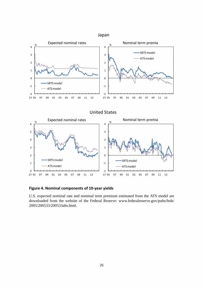
As stated above, the parameters and factors estimated from the standard ATS
models are biased due to ignoring the zero lower bound constraint. Figure 4 compares
the 10-year expected nominal rates and nominal term premia estimated from our SRTS
model with those from the ATS models. We reproduce and estimate the ATS models 17 Note that, in a multi-factor SRTS model, the absolute value of the shadow rate in the negative direction does not directly link to the market-expected duration of zero interest rates (see Ichiue and Ueno, 2007). This is because the expected future path of the nominal short rate depends not only on the level of the shadow rate but also on the combination of latent factors.
14
discussed in Ichiue and Ueno (2013) for Japan and in Kim and Wright (2005) for the
United States, respectively. Note that the nominal and real term premia in Figures 4 to 7
include the estimation errors of the nominal and real yields, respectively. For both
countries, the expected nominal rates estimated from the ATS models are constantly
higher than those from the SRTS model. The deviation tends to be large when the policy
rate is close to zero. For Japan, there has been a constant deviation of 80 basis points
since the 2000s, except for the period from 2006 to 2008 when the Bank of Japan raised
its policy rate. For the United States, the deviation became larger in 2009 when the
Federal Reserve introduced its zero interest rate policy, and reached the recent high of
90 basis points in 2013.
In contrast to the nominal expected rates, the nominal term premia estimated from
the ATS models are lower than those estimated from the SRTS model. For Japan and the
United States, both types of estimates show a similar declining trend during the
post-Lehman-shock period, partly due to the central banks' large-scale asset purchases,
but the pace of decline in the nominal term premium estimated from the ATS models is
more rapid than their counterparts. This indicates that the ATS models are likely to
exaggerate the term premium effects of the central banks' asset purchases. Correcting
the estimation bias makes a significant difference in the current context.
Characteristics of the estimated components
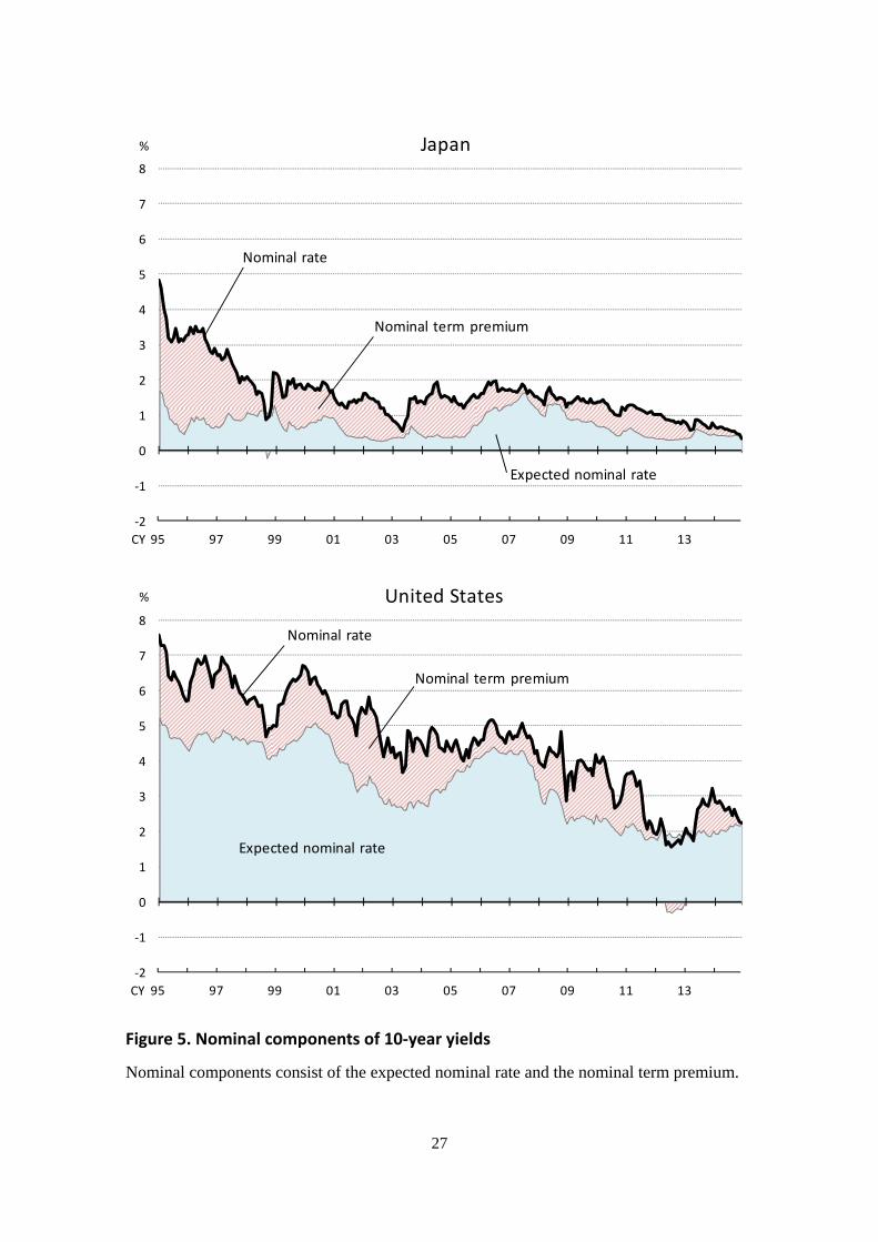
Long-term JGB and U.S. Treasury yields have been at historically low levels for
almost two decades. Figure 5 suggests that expected nominal rates have played a key
role in the long-lasting low yields. Japan's considerably low interest rates have reflected
the low and stable expected nominal rate. In the United States, the declining expected
nominal rate has contributed to the downward trend in Treasury yields. Focusing on the
post-Lehman-shock period, the central banks' monetary easing has further pushed down
the long-term yields. In addition to the lower expected nominal rate, the fall in the
nominal term premium has been driving down long-term yields. Toward the end of 2014,
the 10-year JGB and U.S. Treasury yields reached a range of 0.0-0.5 percent and around
2.0 percent, respectively.

15
To examine the bond yield dynamics in detail during the post-Lehman-shock
period, we conduct full decomposition of long-term yields into four components. Figure
6 shows the estimated components of the 10-year JGB and U.S. Treasury yields:
expected real rate, real term premium, expected inflation, and inflation risk premium.
One of the features common to Japan and the United States is the steady decline in the
expected real rate. The expected real rate is basically influenced by monetary policy, i.e.,
both the current policy stance and market participants' view of how the policy will
evolve. The low level of the expected real rate, currently negative in Japan, reflects the
market participants' view that monetary policy will remain accommodative for a while.
Another feature is the downward move in the real term premium after the Lehman
shock. Japan's real term premium, constantly positive through 2012, dropped sharply to
around zero percent in 2013. U.S. real term premium, though relatively volatile, moved
downward and temporarily hit negative levels during the 2011-2013 period. The real
term premium generally reflects the real-term interest-rate risk – a wide variety of risks
other than inflation risks – as well as investors' preference for safe assets and various
other factors including the central banks' policy actions. The recent fall in the real term
premium mainly reflects the central banks' large-scale asset purchases, which are in
effect through both a scarcity channel and a duration channel by tightening
supply-demand conditions in their government bond markets.18 A decline in future
uncertainty, suggested by the historically low volatility of long-term yields, may also
contribute to the lower real term premium.
While the real components exhibit similar development for JGB and U.S. Treasury
yields, the inflation components, i.e., expected inflation and inflation risk premium,
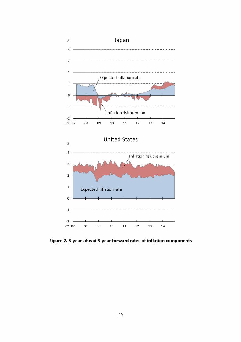
show large differences between the two. In the United States, both the expected inflation
and the inflation risk premium – expected future path of inflation and compensation for
future uncertainty on inflation, respectively – are almost constant in the positive
territory, implying that U.S. inflation expectations are more or less anchored. In
18 The policy effects of the central banks' asset purchases are estimated from the ATS models by, e.g., Gagnon et al. (2011), Joyce et al. (2011), D'Amico et al. (2012), Hamilton and Wu (2012), and Bauer and Rudebusch (2014).
16
particular, the 5-year ahead 5-year forward rate of expected inflation depicted in Figure
7 is notably stable at around 2 percent.
In Japan, the following two changes in the dynamics of inflation expectations have
contributed to an upward movement of the inflation components in recent years. First,
the 5-year ahead 5-year forward rate of expected inflation remained at almost zero
percent after the Lehman shock, but started to increase in 2012. Second, the negative
forward rate of the inflation risk premium has disappeared since 2013.19 Although the
expected inflation has not yet reached the Bank of Japan's price stability target of 2
percent, these two changes imply that market concerns over deflation have subsequently
weakened. Our estimates of inflation components closely match the movements in the
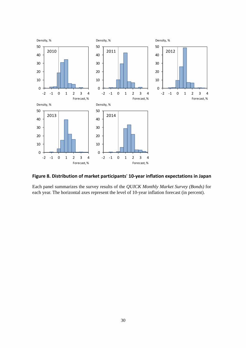
survey measures of market expectations on future inflation. Figure 8 shows the
distribution of the 10-year forecasts for the consumer price index, all items less fresh
food, which are reported by the QUICK Monthly Market Survey.20 Since 2013, more
respondents have forecasted price increases than declines and the distribution skew has
shifted to the inflationary side (Nishiguchi et al., 2014). This suggests that few market
participants think there is a risk of deflation or zero inflation in the future.
4. Concluding remarks
From both a practical and academic viewpoint, it is important to extract the unbiased
information contained in market yield curves. Nevertheless, the standard ATS models
are subject to estimation bias due to ignoring the zero lower bound constraint, and could
produce misleading results. We corrected this bias using the extended SRTS model for
nominal and real yields, and reexamined the dynamics of long-term yields. To our
knowledge, this is the first attempt to fully decompose nominal yields into four
components including the inflation risk premium under the zero lower bound constraint.
19 Long-term inflation risk premia estimated in the literature are almost always positive for the United States, the United Kingdom, and the euro area before the Lehman shock (D'Amico et al., 2010; García and Werner, 2010; and Joyce et al., 2010). 20 The survey is conducted monthly by QUICK Corporation. Each round of the survey has about 200 respondents. For this analysis, panel data on individual forecasts were kindly provided by QUICK Corporation.
17
The empirical analysis applying the proposed model to Japan's and U.S. yield curves
confirms that our model successfully avoids the estimation bias and provides reasonable
estimates at or around the zero lower bound.
The SRTS model in this paper does not explicitly incorporate macroeconomic
variables in the factors driving the term structure and dynamics of the yields. This
means that the model cannot directly assess what kind of news shock affects the
movement of the yield components. It is important to quantitatively measure the
response of the yield components to information about economic and price
developments as well as the central bank's policy actions, which remains as a future
work.
18
References
Adrian, T., and H. Wu (2009), "The term structure of inflation expectations," Federal
Reserve Bank of New York Staff Report, No. 362.
Adrian, T., R. K. Crump, and E. Moench (2013), "Pricing the term structure with linear
regressions," Journal of Financial Economics, 110, pp. 110-138.
Ahn, D., R. F. Dittmar, and A. R. Gallant (2002), "Quadratic term structure models: Theory
and evidence," Review of Financial Studies, 15, pp. 243-288.
Ang, A., G. Bekaert, and M. Wei (2008), "The term structure of real rates and expected
inflation," Journal of Finance, 63, pp. 797-849.
Bank of Japan (2009), Financial Markets Report: Developments in the second half of 2008.
Bauer, M. D., and G. D. Rudebusch (2014), "The signaling channel for Federal Reserve
bond purchases," International Journal of Central Banking, 10, pp. 233-289.
Bernanke, B. (2013a), "Long-term interest rates," remarks at the Annual
Monetary/Macroeconomics Conference: The Past and Future of Monetary Policy,
March 1, 2013.
Bernanke, B. (2013b), Statement by Ben S. Bernanke Chairman Board of Governors of the
Federal Reserve System before the Joint Economic Committee, May 22, 2013.
Black, F. (1995), "Interest rates as options," Journal of Finance, 50, pp. 1371-1376.
Campbell, J., A. Sunderam, and L. Viceira (2009), "Inflation bets or deflation hedges? The
changing risks of nominal bonds," NBER Working Paper, No. 14701.
Chernov, M., and P. Mueller (2012), "The term structure of inflation expectations," Journal
of Financial Economics, 106, pp. 367-394.
Christensen, J. H. E., J. A. Lopez, and G. D. Rudebusch (2010), "Inflation expectations and
risk premiums in an arbitrage-free model of nominal and real bond yields," Journal of
Money, Credit and Banking, 42(s1), pp. 143-178.
Christensen, J. H. E., and G. D. Rudebusch (2013), "Modeling yields at the zero lower
bound: Are shadow rates the solution?" Federal Reserve Bank of San Francisco
Working Paper Series, 2013-39.
––––––––––––––––––––––––––––––––––––– (2014), "Estimating shadow-rate term
structure models with near-zero yields," Journal of Financial Econometrics,
forthcoming.
19
Dai, Q., and K. J. Singleton (2000), "Specification analysis of affine term structure models,"
Journal of Finance, 55, pp. 1943-1978.
D'Amico, S., W. English, D. Lopez-Salido, and E. Nelson (2012), "The Federal Reserve's
large-scale asset purchase programmes: Rationale and effects," Economic Journal, 122,
pp. 415-446.
D'Amico, S., D. H. Kim, and M. Wei (2010), "Tips from TIPS: The informational content of
Treasury Inflation-Protected Security prices," Finance and Economics Discussion
Series, 2010-19, Federal Reserve Board.
Duffie, D. (2001), Dynamic Asset Pricing Theory, 3rd. edition, Princeton University Press.
Duffie, D., and R. Kan (1996), "A yield-factor model of interest rates," Mathematical
Finance, 6, pp. 379-406.
Gagnon, J., M. Raskin, J. Remache, and B. Sack (2011), "The financial market effects of the
Federal Reserve's large-scale asset purchases," International Journal of Central
Banking, 7, pp. 3-43.
García, J. A., and T. Werner (2010), "Inflation risks and inflation risk premia," European
Central Bank Working Paper Series, No. 1162.
Guimarães, R. (2014), "Expectations, risk premia and information spanning in dynamic
term structure model estimation," Bank of England Working Paper, No. 489.
Gürkaynak, R. S., B. Sack, and J. Wright (2007), "The US Treasury yield curve: 1961 to the
present," Journal of Monetary Economics, 54, pp. 2291-2304.
–––––––––––––––––––––––––––––––– (2010), "The TIPS yield curve and inflation
compensation," American Economic Journal: Macroeconomics, 2, pp. 70-92.
Hamilton, J. D., and J. C. Wu (2012), "The effectiveness of alternative monetary policy
tools in a zero lower bound environment," Journal of Money, Credit and Banking,
44(s), pp. 3-46.
Haubrich, J., G. Pennacchi, and P. Ritchken, (2012), "Inflation expectations, real rates, and
risk premia: Evidence from inflation swaps," Review of Financial Studies, 25, pp.
1588-1629.
Hördahl, P., and O. Tristani, (2010), "Inflation risk premia in the US and the euro area,"
European Central Bank Working Paper Series, No. 1270.
20
Hördahl, P., and O. Tristani (2012), "Inflation risk premia in the term structure of interest
rates," Journal of the European Economic Association, 10, pp. 634-657.
Ichiue, H., and Y. Ueno (2007), "Equilibrium interest rate and the yield curve in a low
interest rate environment," Bank of Japan Working Paper Series, No. 07-E-18.
–––––––––––––––––––– (2013), "Estimating term premia at the zero bound: An analysis of
Japanese, US, and UK yields," Bank of Japan Working Paper Series, No. 13-E-8.
Joyce, M., P. Lildholdt, and S. Sorensen (2010), "Extracting inflation expectations and
inflation risk premia from the term structure: A joint model of the UK nominal and real
yield curves," Journal of Banking and Finance, 34, pp. 281-294.
Joyce, M., M. Tong, and R. Woods (2011), "The United Kingdom's quantitative easing
policy: Design, operation and impact," Bank of England Quarterly Bulletin, 2011, 3rd
Quarter, 200-212.
Kikuchi, K. (2012), "Design and estimation of a quadratic term structure model with a
mixture of normal distributions," IMES Discussion Paper Series, 2012-E-8, Bank of
Japan.
Kim, D. H., and K. J. Singleton (2012), "Term structure models and the zero bound: An
empirical investigation of Japanese yields," Journal of Econometrics, 170, pp. 32-49.
Kim, D. H., and J. H. Wright (2005), "An arbitrage-free three-factor term structure model
and the recent behavior of long-term yields and distant-horizon forward rates," Finance
and Economics Discussion Series, 2005-33, Federal Reserve Board.
Koeda, J. (2013), "Endogenous monetary policy shifts and the term structure: Evidence
from Japanese government bond yields," Journal of the Japanese and International
Economies, 29, pp. 170-188.
Leippold, M., and L. Wu (2003), "Design and estimation of quadratic term structure
models," European Finance Review, 7, pp. 47-73.
McCulloch, J. (1990), "U.S. government term structure data, 1947-1987," in B. M.
Friedman, and F. Hahn, eds., Handbook of Monetary Economics I, pp. 672-715.
Nishiguchi, S., J. Nakajima, and K. Imakubo (2014), "Disagreement in households' inflation
expectations and its evolution," Bank of Japan Review, No. 2014-E-1.
21
Table 1. RMSEs for nominal yields
bps
2‐year 5‐year 7‐year 10‐year
All periods 5 2 5 7
Before 2007/Mar 4 2 4 8
After 2007/Apr 5 1 5 6
bps
2‐year 5‐year 7‐year 10‐year
All periods 9 2 1 16
Before 2004/Dec 9 2 1 9
After 2005/Jan 9 3 1 19
Japan
United States
22
Table 2. RMSEs for nominal yields: preceding models
Maximum RMSEs are reported in each model.
Estimation periods bps
Ichiue and Ueno (2013) Japan 1990/Jan ‐ 2013/Mar 15
U.S. 1990/Jan ‐ 2013/Mar 13
U.K. 1990/Jan ‐ 2013/Mar 24
Kim and Singleton (2012) U.S. 1995/Jan ‐ 2008/Mar 12
Estimation periods bps
D'Amico et al. (2010) U.S. 1990/Jan ‐ 2007/Mar 5
Christensen et al. (2010) U.S. 1995/Jan ‐ 2008/Mar 11
Joyce et al. (2010) U.K. 1992/Oct ‐ 2008/Feb 15
SRTS models for nominal yields
ATS models for nominal and real yields
23
Figure 1. Components of nominal yields
Realterm premium
Nominal rateExpected
nominal rateNominal
term premium
Real rateExpectedreal rate
Inflation swap rate
Expectedinflation rate
Inflationrisk premium
= ==
=
=
=
+
+
+
+ ++
24
Figure 2. Yield data
Direct effects of the consumption tax hikes on Japan's inflation swap rate are adjusted.
0
1
2
3
4
5
6
95 97 99 01 03 05 07 09 11 13
10yr
7yr
5yr
2yr
O/N
%Nominal yields
CY
Japan United States
0
2
4
6
8
10
95 97 99 01 03 05 07 09 11 13
10yr
5yr
2yr
1yr
O/N
%Nominal yields
CY
‐2
‐1
0
1
2
3
4
95 97 99 01 03 05 07 09 11 13
10yr
7yr
5yr
2yr
%Real yields
CY
‐4
‐2
0
2
4
6
95 97 99 01 03 05 07 09 11 13
10yr
5yr
2yr
1yr
%Real yields
CY
‐4
‐3
‐2
‐1
0
1
2
95 97 99 01 03 05 07 09 11 13
10yr
7yr
5yr
2yr
% Inflation swap rates
CY
‐6
‐4
‐2
0
2
4
95 97 99 01 03 05 07 09 11 13
10yr
5yr
2yr
1yr
% Inflation swap rate
CY

25
Figure 3. Estimated shadow rates
‐6
‐4
‐2
0
2
4
6
8
95 97 99 01 03 05 07 09 11 13
%Japan
CY
‐6
‐4
‐2
0
2
4
6
8
95 97 99 01 03 05 07 09 11 13
%United States
CY
26
Figure 4. Nominal components of 10‐year yields
U.S. expected nominal rate and nominal term premium estimated from the ATS model are downloaded from the website of the Federal Reserve: www.federalreserve.gov/pubs/feds/ 2005/200533/200533abs.html.
‐2
‐1
0
1
2
3
4
95 97 99 01 03 05 07 09 11 13
SRTS model
ATS model
%Expected nominal rates
‐2
‐1
0
1
2
3
4
95 97 99 01 03 05 07 09 11 13
SRTS model
ATS model
%Nominal term premia
Japan
CYCY
0
1
2
3
4
5
6
95 97 99 01 03 05 07 09 11 13
SRTS model
ATS model
%Expected nominal rates
‐2
‐1
0
1
2
3
4
95 97 99 01 03 05 07 09 11 13
SRTS model
ATS model
%Nominal term premia
United States
CY CY
27
Figure 5. Nominal components of 10‐year yields
Nominal components consist of the expected nominal rate and the nominal term premium.
‐2
‐1
0
1
2
3
4
5
6
7
8
95 97 99 01 03 05 07 09 11 13
Nominal term premium
Expected nominal rate
Nominal rate
Japan%
CY
‐2
‐1
0
1
2
3
4
5
6
7
8
95 97 99 01 03 05 07 09 11 13
Nominal term premium
Expected nominal rate
Nominal rate
United States%
CY

28
Figure 6. Real and inflation components of 10‐year yields
Real components consist of the expected real rate and the real term premium, while inflation components consist of the expected inflation rate and the inflation risk premium.
‐2
‐1
0
1
2
3
4
5
07 08 09 10 11 12 13 14
Real term premium
Expected inflation rate
Expected real rate
Inflation risk premium
Nominal rate
United States%
CY
‐2
‐1
0
1
2
3
4
5
07 08 09 10 11 12 13 14
Real term premium Expected inflation rate
Expected real rate Inflation risk premium
Nominal rate
Japan%
CY
29
Figure 7. 5‐year‐ahead 5‐year forward rates of inflation components
‐2
‐1
0
1
2
3
4
07 08 09 10 11 12 13 14
Japan%
Expected inflation rate
Inflation risk premium
CY
‐2
‐1
0
1
2
3
4
07 08 09 10 11 12 13 14
United States %
Expected inflation rate
Inflation risk premium
CY
30
Figure 8. Distribution of market participants' 10‐year inflation expectations in Japan
Each panel summarizes the survey results of the QUICK Monthly Market Survey (Bonds) for each year. The horizontal axes represent the level of 10-year inflation forecast (in percent).
0
10
20
30
40
50
‐2 ‐1 0 1 2 3 4
Density, %
2010
Forecast,%
0
10
20
30
40
50
‐2 ‐1 0 1 2 3 4
Density, %
2011
Forecast,%
0
10
20
30
40
50
‐2 ‐1 0 1 2 3 4
Density, %
2012
Forecast,%
0
10
20
30
40
50
‐2 ‐1 0 1 2 3 4
Density, %
2013
Forecast,%
0
10
20
30
40
50
‐2 ‐1 0 1 2 3 4
Density, %
2014
Forecast,%