ENSO Transition, Duration, and Amplitude Asymmetries: Role of the NonlinearWind Stress Coupling in a Conceptual Model
KIT-YAN CHOI
Princeton University, Princeton, New Jersey
GABRIEL A. VECCHI AND ANDREW T. WITTENBERG
Geophysical Fluid Dynamics Laboratory, and Princeton University, Princeton, New Jersey
(Manuscript received 18 January 2013, in final form 31 May 2013)
ABSTRACT
The El Ni~no–Southern Oscillation (ENSO) exhibits well-known asymmetries: 1) warm events are stronger
than cold events, 2) strong warm events are more likely to be followed by cold events than vice versa, and 3)
cold events are more persistent than warm events. Coupled GCM simulations, however, continue to un-
derestimate many of these observed features.
To shed light on these asymmetries, the authors begin with a widely used delayed-oscillator conceptual
model for ENSO and modify it so that wind stress anomalies depend more strongly on SST anomalies
(SSTAs) duringwarm conditions, as is observed. Then the impact of this nonlinearity onENSO is explored for
three dynamical regimes: self-sustained oscillations, stochastically driven oscillations, and self-sustained os-
cillations disrupted by stochastic forcings. In all three regimes, the nonlinear air–sea coupling preferentially
strengthens the feedbacks (both positive and delayed negative) during the ENSOwarm phase—producing El
Ni~nos that grow to a larger amplitude and overshoot more rapidly and consistently into the opposite phase,
than do the La Ni~nas. Finally, the modified oscillator is applied to observational records and to control
simulations from two global coupled ocean–atmosphere–land–ice models [Geophysical Fluid Dynamics
Laboratory Climate Model version 2.1 (GFDL CM2.1) and version 2.5 (GFDL CM2.5)] to elucidate the
causes of their differing asymmetries.
1. Introduction
Fluctuations of the El Ni~no–Southern Oscillation
(ENSO) involve coupled changes to the ocean and at-
mosphere. During the warm phase of ENSO, the pre-
vailing easterly winds over the central Pacific weaken;
these westerly wind anomalies advect warm surface
water toward the east, reduce the zonal slope of the
thermocline, and inhibit the upwelling of cold water in
the eastern Pacific, which feeds back positively on the
warming of surface water in the eastern Pacific and al-
lows small perturbations to grow. This positive feedback
is also known as the Bjerknes feedback (Bjerknes 1969).
To first approximation, La Ni~na (the cold phase) anom-
alies are roughly the opposite of those of El Ni~no (Larkin
andHarrison 2002, hereafter LH2002). Theories proposed
to explain the termination of El Ni~no (La Ni~na) and its
transition into the opposite phase include the reflection
of oceanic internal waves at the eastern and western
boundaries (Suarez and Schopf 1988; Battisti and Hirst
1989, hereafter BH1989), recharge and discharge of equa-
torial warm water due to Sverdrup balance (Jin 1997),
western Pacific wind-forced Kelvin waves (Weisberg and
Wang 1997), and anomalous zonal temperature advec-
tion by oceanic currents (Picaut et al. 1997). These the-
ories agree that oceanic adjustments result in delayed
negative feedbacks that explain the turnabout between
ElNi~no and LaNi~na, with simple models illustrating how
these mechanisms can result in oscillatory behavior for
ENSO. Although nonlinearity has been shown to impact
the growth and decay of El Ni~no (Tziperman et al. 1997;
Gebbie et al. 2007; Vecchi 2006; Vecchi and Harrison
2006), linear techniques that are widely used for studying
ENSO, such as empirical orthogonal function (EOF)
analysis and linear regression, tend to treat El Ni~no and
La Ni~na as simple mirror images of each other.
Corresponding author address: Kit-Yan Choi, Princeton Uni-
versity, 201 Forrestal Road, Princeton, NJ 08540.
E-mail: [email protected]
9462 JOURNAL OF CL IMATE VOLUME 26
DOI: 10.1175/JCLI-D-13-00045.1
� 2013 American Meteorological Society
For all of the approximate symmetries of El Ni~no and
La Ni~na events, considerable asymmetry does exist.Most
noted in past literature is the amplitude asymmetry of
ENSO, namely that El Ni~no tend to be stronger than La
Ni~na (Burgers and Stephenson 1999). Several oceanic
mechanisms have been proposed for this asymmetry:
nonlinear dynamical heating (Jin et al. 2003; An and Jin
2004) and negative feedback owing to tropical instability
waves that are stronger during La Ni~na (Wang and
McPhaden 2000; Vialard et al. 2001). A common element
of all of these proposed mechanisms is their inherent
oceanic origin.
Other studies have drawn attention to the asymmetric
atmospheric response to sea surface temperature changes.
Kang and Kug (2002) studied a hybrid atmosphere–ocean
coupled model and suggested that the relatively weaker
sea surface temperature anomalies (SSTAs) and shorter
duration for La Ni~na are attributable to the westward
shift of the wind stress anomalies (Hoerling et al. 1997).
Philip and van Oldenborgh (2009) and Frauen and
Dommenget (2010) found that a nonlinear zonal wind
response to the opposite sign SST anomalies may have
an important influence on the SST skewness in the east-
ern tropical Pacific. Dommenget et al. (2013) suggest that
the skewness in SST is related to the asymmetries in the
pattern shape and the time evolution of ENSO events
that can be partially attributed to the nonlinear response
of the zonal wind to SST anomalies. Nonlinear relation-
ships between the seasonal cycle andENSO aswell as the
origins of ENSO phase locking to the seasonal cycle were
also studied (Harrison and Vecchi 1999; Galanti and
Tziperman 2000; Tziperman et al. 1997; Galanti et al.
2002).
In addition to amplitude asymmetry, there are other
differences in the evolution of El Ni~no and La Ni~na.
LH2002 characterized differences in the life cycles of the
warm and cold phases by examining the ENSO behavior
phase by phase. In their appendix, LH2002 note that
warm-to-cold transitions tend to occur within a single
year, with the cold event emerging the year following the
warm event. In contrast, cold-to-warm transitions occur
over 1–3 years. Okumura and Deser (2010) also showed
that there is a robust asymmetry in the duration of El
Ni~no and La Ni~na in observations, with La Ni~na per-
sisting longer, a feature also noted by Kessler (2002).
Subsequently, Okumura et al. (2011) proposed that an
asymmetric wind response due to delayed SST forcing in
the Indian Ocean acts to prolong La Ni~na.
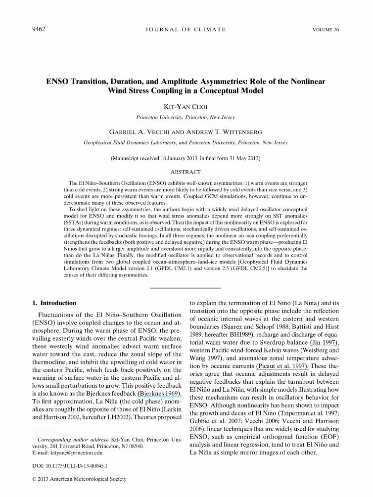
Various observational datasets of Pacific surface wind
stress support the hypothesis that during ENSO the wind
stress response to the SST anomalies is weaker in the
cold phase than in the warm phase. Figure 1 shows re-
gression coefficients of zonal wind stress anomalies onto
the Ni~no-3.4 SSTA index (area average of SST anoma-
lies at 58S–58N, 1708–1208W) during warm and cold
conditions for the Florida State University (FSU) ob-
servational wind product (see section 2). The asymmetry
in the sensitivity is also evident in other estimates of
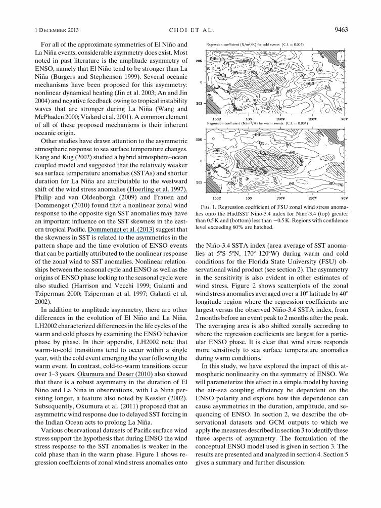
wind stress. Figure 2 shows scatterplots of the zonal
wind stress anomalies averaged over a 108 latitude by 408longitude region where the regression coefficients are
largest versus the observed Ni~no-3.4 SSTA index, from
2months before an event peak to 2months after the peak.
The averaging area is also shifted zonally according to
where the regression coefficients are largest for a partic-
ular ENSO phase. It is clear that wind stress responds
more sensitively to sea surface temperature anomalies
during warm conditions.
In this study, we have explored the impact of this at-
mospheric nonlinearity on the symmetry of ENSO. We
will parameterize this effect in a simple model by having
the air–sea coupling efficiency be dependent on the
ENSO polarity and explore how this dependence can
cause asymmetries in the duration, amplitude, and se-
quencing of ENSO. In section 2, we describe the ob-
servational datasets and GCM outputs to which we
apply themeasures described in section 3 to identify these
three aspects of asymmetry. The formulation of the
conceptual ENSO model used is given in section 3. The
results are presented and analyzed in section 4. Section 5
gives a summary and further discussion.
FIG. 1. Regression coefficient of FSU zonal wind stress anoma-
lies onto the HadISST Ni~no-3.4 index for Ni~no-3.4 (top) greater
than 0.5K and (bottom) less than20.5K. Regions with confidence
level exceeding 60% are hatched.
1 DECEMBER 2013 CHO I ET AL . 9463
FIG. 2. Regression coefficient of the area-averaged zonal wind stress anomalies onto the Ni~no-3.4 index for Ni~no-3.4(top) greater than 0.5K or (bottom) less than20.5K. The HadISSTNi~no-3.4 index is used for the FSU and ERA-40
regression analysis. Reanalysis wind stress anomalies are regressed onto the reanalysis Ni~no-3.4 indices for MERRA
and NCEP-1, respectively. Model wind stress anomalies are regressed onto the model Ni~no-3.4 index; area averages
of the wind stress are computed within 408 longitude boxes from 58S to 58N where the regression coefficient is the
largest across the equatorial Pacific domain. For warm events, wind stress anomalies are averaged within boxes at
1778–1378W (FSU), 1768E–1448W (ERA-40), 1768–1368W (NCEP-1), 1798–1398W (MERRA), 1678E–1538W(CM2.1), and 1708E–1508W (CM2.5). For cold events, the box sits at 1718E–1498W (FSU), 1538E–1678W (ERA-40),
1608E–1608W (NCEP-R1), 1678E–1538W (MERRA), 1408E–1808 (CM2.1), and 1408E–1808 (CM2.5).
9464 JOURNAL OF CL IMATE VOLUME 26
2. Data sources
a. SST data
There are uncertainties in past reconstructions of the
tropical Pacific SST (Vecchi et al. 2008) and we therefore
explore two SST datasets: the Hadley Centre Sea Ice and
Sea Surface Temperature dataset (HadISST) and the
extended reconstructed SST version 3b (ERSST).
1) HADISST
The HadISST dataset for 1880–2012 (Rayner et al.
2003) is used for computing the Ni~no-3.4 SSTA index.
We examine the historical record entirely as well as in
segments. Monthly climatologies are computed over the
period of the time series sampled, and the anomalies are
computed by subtracting the climatologies from the orig-
inal record. The HadISST Ni~no-3.4 SST anomalies have
increased by 0.28 from 1880 to 2012.
2) ERSST V3B
ERSST version 3b (Smith et al. 2008) provided by the
National Oceanic and Atmospheric Administration is
used as another long-term SST observational record to
compare with HadISST. The dataset spans from 1854 to
present. In the current study, the time series from 1880
to 2012 is used since the strength of the signal becomes
more consistent after 1880. This version of SST analysis
uses in situ SST data and improved statistical methods.
Unlike version 3, satellite data, which that causes a small
cold bias, is not used in version 3b. From 1880 to 2012,
ERSST Ni~no-3.4 SST anomalies have increased by 0.68.The warming trends in the HadISST and ERSST
products are included in the analysis presented below.
The Ni~no-3.4 temperature anomalies are also smoothed
using a running 5-month boxcar average before analysis.
We will discuss the sensitivity of the results to whether
the time series is detrended or not.
b. Surface wind stress estimates
There are also large uncertainties in reconstructions
of wind stress over the Pacific (Wittenberg 2004), so we
use multiple wind stress estimates in our analysis. Ob-
servational datasets used here for the wind stress re-
sponse analysis are the Center for Ocean–Atmospheric
Prediction Studies (COAPS) third-generation Florida
State University objectively gridded Pacific monthly
mean in situ flux products (FSU3) (Bourassa et al. 2005)
from1987 to 2004; the 40-yrEuropeanCentre forMedium-
Range Weather Forecast (ECMWF) Re-Analysis (ERA-
40) (Uppala et al. 2005) 6-hourlymomentum stress product
from September 1957 to August 2002; ECMWF Interim
Re-Analysis (ERA-Interim) (Dee and Uppala 2009)
from 1979 to 2011; the National Aeronautics and Space
Administration Modern-Era Retrospective Analysis for
Research andApplications (MERRA) (Rienecker et al.
2011) from 1979 to 2010; and the National Centers for
Environmental Prediction–National Center for Atmo-
spheric Research (NCEP–NCAR) reanalysis (NCEP-1)
(Kalnay et al. 1996; Kistler et al. 2001) from 1948 to
2011.
c. Coupled GCMs
1) GFDL CM2.1
The Geophysical Fluid Dynamics Laboratory (GFDL)
Climate Model version 2.1 (CM2.1) is a global coupled
atmosphere–ocean–land–ice GCM. The detailed for-
mulations are described by Delworth et al. (2006, and
references therein). Wittenberg et al. (2006) describes
the behavior of ENSO in this model. The CM2.1 has
taken part in phases 3 and 5 of the Coupled Model In-
tercomparison Project (CMIP3 and CMIP5) and the
Fourth Assessment of the Intergovernmental Panel on
Climate Change (IPCC). In this study, we use the monthly
mean output of the preindustrial control experiment in-
tegrated for 4000 years with fixed 1860 estimates of solar
irradiance, land cover, and atmospheric composition.
The long run providesmore than 300 El Ni~no and 300 La
Ni~na events and thus allows statistically significant analysis
of the behavior of the simulated ENSO. The description
of the interdecadal variability of ENSO for the first 2200
years of this experiment is described inWittenberg (2009).
2) GFDL CM2.5
The GFDL Climate Model version 2.5 (CM2.5) is a
newer higher-resolution (atmosphere/land horizontal
resolution is 0.58 instead of 28; ocean/sea ice resolution is
about 0.258 instead of 18) global coupled GCM based on
CM2.1. The two models are initialized and forced in
a similar fashion. The resolutions of the atmosphere and
ocean components in CM2.5 are increased. A smaller
viscosity is used in CM2.5. Parameterized eddy mixing is
excluded in the CM2.5 ocean, while it is included in
CM2.1. Further details on CM2.5 and comparisons with
CM2.1 are documented in Delworth et al. (2012). The
data used in this study are based on a 260-yr control ex-
periment using fixed 1990 estimates of solar irradiance,
land cover, and atmospheric composition. The 37 El Ni~nos
and 34 La Ni~nas are identified in this experiment.
3) COMPARISON OF THE SIMULATED ENSO IN
CM2.5 AND CM2.1 WITH OBSERVATIONS
Delworth et al. (2012) describe how the simulated
ENSO in CM2.5 compares to CM2.1 and observations.
More detailed descriptions of the CM2.1 ENSO be-
havior can be found inWittenberg et al. (2006). Here we
summarize some of their results.
1 DECEMBER 2013 CHO I ET AL . 9465

TheENSO amplitude in CM2.5 is weaker and is closer
to observations, while CM2.1 tends to simulate ENSO
events that are too strong. While both models have
equatorial Pacific SST anomalies that extend too far to
the west, this bias is reduced in CM2.5.
Both models have problems simulating the seasonal
phase locking of ENSO. The CM2.1 ENSO shows al-
most no seasonal phase locking, except that the Ni~no-3.4
index has a slight tendency to peak between October
and February and strong events tend to lock better to the
seasonal cycle. The CM2.5 Ni~no-3.4 index has better
phase locking compared to CM2.1 but is still weaker and
later than observations by about a month.
At interannual time scales, the spectrum of tropical
Pacific SSTs in CM2.5 is too concentrated at about 2.5 yr.
CM2.1 shows a broader and more realistic spectrum but
is stronger than the observations at interannual time
scales. Accordingly, the ENSO in CM2.5 is noticeably
more regular than CM2.1 and the observed. However, the
lengths of observational records are short, so the spectra
in this frequency band are uncertain (Wittenberg 2009;
Vecchi and Wittenberg 2010).
3. Methods
a. The conceptual ENSO model
Following the delayed-oscillator model proposed by
BH1989, which is closely related to the models studied
by Suarez and Schopf (1988) and Zebiak and Cane
(1987), we model ENSO as arriving from two essential
drivers: first, the Bjerknes positive feedback that leads
to instability and, second, a delayed negative feedback
that results in oscillations. We thereby use a conceptual
model of ENSO based on the BH1989 model:
›T
›t52bT1 c0t x(t2 t1)2 d0t x(t2 t2)2 �T3 , (1)
where T is the Ni~no-3.4 SST anomaly; tx is the wind
stress anomaly at the central equatorial Pacific near the
date line; t1 is the time required for wind stress response
to positively feedback to surface temperature T; t2 is the
time required for the negative feedback to enact; t1 is
smaller than t2; b, c0 and d0 are positive scalar parameters;
and � is nonzero when the system is unstable otherwise.
The current settings for t1 and t2 are 1 and 6 months,
which are roughly the times required for the first/second
baroclinic Kelvin wave to propagate eastward from the
date line to theAmerican coasts and the time required for
Rossby waves to propagate westward and reflect back
as Kelvin waves to the eastern Pacific (Harrison and
Giese 1988; Harrison and Vecchi 1999). The qualitative
conclusion is unchanged if different values of t1 and t2 are
used as long as t2 . t1. If t15 0, one recovers the BH1989
formulation.
The first term on the rhs of Eq. (1) is a qualitative
representation of local dampings of T due to air–sea
fluxes, the mean zonal advection of the anomalous zonal
temperature gradient, and the mean vertical advection
of the anomalous temperature gradient that depends on
T. Guided by BH1989 and regression analysis on these
processes at the eastern Pacific, the value of b is kept
fixed at 0.24 month21 throughout the entire study.
The second and the third terms are the positive and
the delayed-negative feedbacks. Each of these two terms
incorporates the anomalous zonal advection of the mean
zonal temperature gradient, (part of the) mean vertical
advection of the anomalous vertical temperature gradi-
ent, and the anomalous vertical advection of the mean
vertical temperature gradient.
By construction, Eq. (1) gives a symmetric oscillator
in which warm and cold maxima have equal persistence,
frequencies, and amplitudes. To break the symmetry, we
write tx 5 tx(T) such that the wind stress anomalies
respondmore sensitively to warm SST anomalies than to
cold SST anomalies. For simplicity, we write tx as a
piecewise linear function of T; that is,
tx5 g(T1 rjTj) , (2)
where g (PaK21) and r (nondimensional) are both
scalar parameters. For r positive and less than 1, wind
stress anomalies are stronger for the same degree of
positive T than negative T.
From the regression analysis of wind stress response
to SST anomalies (Fig. 1), we can estimate r from the
difference in the regression slopes:
r5sw 2 scsw 1 sc
, (3)
where sw and sc are the slopes for warm and cold events,
respectively.
Table 1 summarizes the value of r estimated from
different datasets. Most datasets produce an r of about
20%with the exception of NCEP-1. This agrees with the
suggestion made by Wittenberg (2004) that FSU is rec-
ommended over NCEP-1 for extended studies of ENSO
since the former dataset agrees better with other ob-
servations and updated analysis. Why the NCEP-1 does
not show the nonlinear relationship between the zonal
wind stress and SST during ENSO, as is seen in other
datasets, is unclear.
In addition to the asymmetry in the intensity of the
wind response, it is likely that the zonal shift in the wind
stress patterns (Fig. 1) between El Ni~no and La Ni~na
9466 JOURNAL OF CL IMATE VOLUME 26
may also be an important feature of ENSO (Kang and
Kug 2002). However, we forgo investigation of pattern
change effects in the present study in order to focus
more intensely on the effects of the wind stress strength
anomaly.
Further regression analysis of the wind stress response
shows that CM2.1 has a large estimated value of r ’46%,much higher than the observed. Conversely, CM2.5
has a smaller value of r (515%).
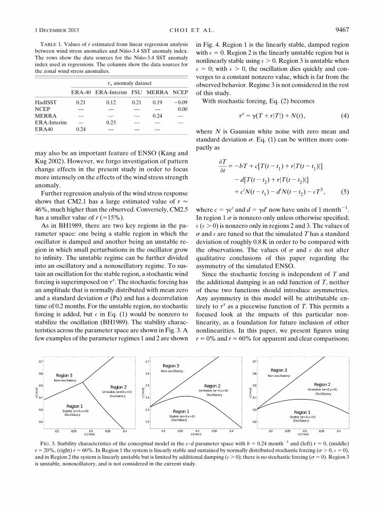
As in BH1989, there are two key regions in the pa-
rameter space: one being a stable region in which the
oscillator is damped and another being an unstable re-
gion in which small perturbations in the oscillator grow
to infinity. The unstable regime can be further divided
into an oscillatory and a nonoscillatory regime. To sus-
tain an oscillation for the stable region, a stochastic wind
forcing is superimposed on tx. The stochastic forcing has
an amplitude that is normally distributed with mean zero
and a standard deviation s (Pa) and has a decorrelation
time of 0.2 months. For the unstable region, no stochastic
forcing is added, but � in Eq. (1) would be nonzero to
stabilize the oscillation (BH1989). The stability charac-
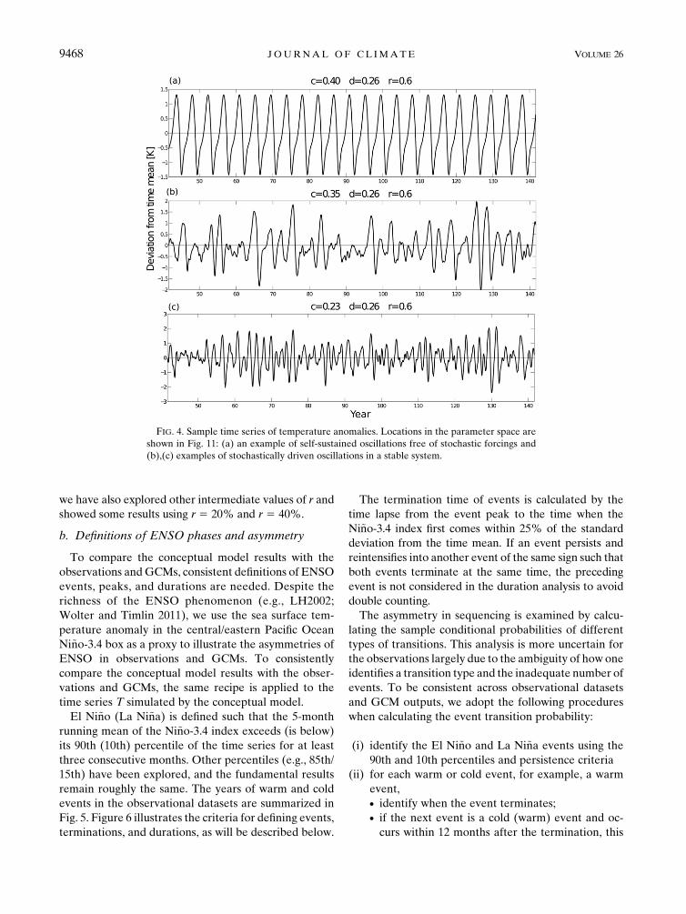
teristics across the parameter space are shown in Fig. 3. A
few examples of the parameter regimes 1 and 2 are shown
in Fig. 4. Region 1 is the linearly stable, damped region
with � 5 0. Region 2 is the linearly unstable region but is
nonlinearly stable using �. 0. Region 3 is unstable when
� 5 0; with � . 0, the oscillation dies quickly and con-
verges to a constant nonzero value, which is far from the
observed behavior. Regime 3 is not considered in the rest
of this study.
With stochastic forcing, Eq. (2) becomes
tx5 g(T1 rjTj)1N(t) , (4)
where N is Gaussian white noise with zero mean and
standard deviation s. Eq. (1) can be written more com-
pactly as
›T
›t52bT1 c[T(t2 t1)1 rjT(t2 t1)j]
2 d[T(t2 t2)1 rjT(t2 t2)j]1 c0N(t2 t1)2 d0N(t2 t2)2 �T3 , (5)
where c5 gc0 and d5 gd0 now have units of 1 month21.
In region 1 s is nonzero only unless otherwise specified;
� (�. 0) is nonzero only in regions 2 and 3. The values of
s and � are tuned so that the simulated T has a standard
deviation of roughly 0.8K in order to be compared with
the observations. The values of s and � do not alter
qualitative conclusions of this paper regarding the
asymmetry of the simulated ENSO.
Since the stochastic forcing is independent of T and
the additional damping is an odd function of T, neither
of these two functions should introduce asymmetries.
Any asymmetry in this model will be attributable en-
tirely to tx as a piecewise function of T. This permits a
focused look at the impacts of this particular non-
linearity, as a foundation for future inclusion of other
nonlinearities. In this paper, we present figures using
r5 0% and r5 60% for apparent and clear comparisons;
TABLE 1. Values of r estimated from linear regression analysis
between wind stress anomalies and Ni~no-3.4 SST anomaly index.
The rows show the data sources for the Ni~no-3.4 SST anomaly
index used in regressions. The columns show the data sources for
the zonal wind stress anomalies.
tx anomaly dataset
ERA-40 ERA-Interim FSU MERRA NCEP
HadISST 0.21 0.12 0.21 0.19 20.09
NCEP — — — — 0.00
MERRA — — — 0.24 —
ERA-Interim — 0.23 — — —
ERA40 0.24 — — —
FIG. 3. Stability characteristics of the conceptual model in the c–d parameter space with b 5 0.24 month21 and (left) r 5 0, (middle)
r5 20%, (right) r5 60%. In Region 1 the system is linearly stable and sustained by normally distributed stochastic forcing (s. 0, �5 0),
and in Region 2 the system is linearly unstable but is limited by additional damping (�. 0); there is no stochastic forcing (s5 0). Region 3
is unstable, nonoscillatory, and is not considered in the current study.
1 DECEMBER 2013 CHO I ET AL . 9467
we have also explored other intermediate values of r and
showed some results using r 5 20% and r 5 40%.
b. Definitions of ENSO phases and asymmetry
To compare the conceptual model results with the
observations andGCMs, consistent definitions of ENSO
events, peaks, and durations are needed. Despite the
richness of the ENSO phenomenon (e.g., LH2002;
Wolter and Timlin 2011), we use the sea surface tem-
perature anomaly in the central/eastern Pacific Ocean
Ni~no-3.4 box as a proxy to illustrate the asymmetries of
ENSO in observations and GCMs. To consistently
compare the conceptual model results with the obser-
vations and GCMs, the same recipe is applied to the
time series T simulated by the conceptual model.
El Ni~no (La Ni~na) is defined such that the 5-month
running mean of the Ni~no-3.4 index exceeds (is below)
its 90th (10th) percentile of the time series for at least
three consecutive months. Other percentiles (e.g., 85th/
15th) have been explored, and the fundamental results
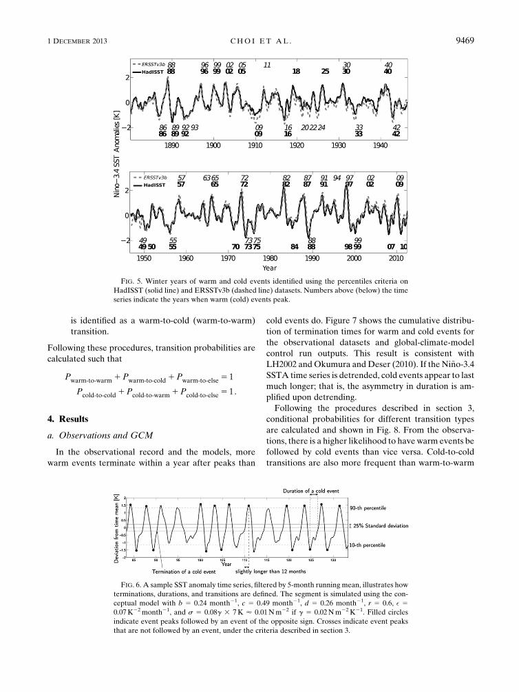
remain roughly the same. The years of warm and cold
events in the observational datasets are summarized in
Fig. 5. Figure 6 illustrates the criteria for defining events,
terminations, and durations, as will be described below.
The termination time of events is calculated by the
time lapse from the event peak to the time when the
Ni~no-3.4 index first comes within 25% of the standard
deviation from the time mean. If an event persists and
reintensifies into another event of the same sign such that
both events terminate at the same time, the preceding
event is not considered in the duration analysis to avoid
double counting.
The asymmetry in sequencing is examined by calcu-
lating the sample conditional probabilities of different
types of transitions. This analysis is more uncertain for
the observations largely due to the ambiguity of how one
identifies a transition type and the inadequate number of
events. To be consistent across observational datasets
and GCM outputs, we adopt the following procedures
when calculating the event transition probability:
(i) identify the El Ni~no and La Ni~na events using the
90th and 10th percentiles and persistence criteria
(ii) for each warm or cold event, for example, a warm
event,d identify when the event terminates;d if the next event is a cold (warm) event and oc-
curs within 12 months after the termination, this
FIG. 4. Sample time series of temperature anomalies. Locations in the parameter space are
shown in Fig. 11: (a) an example of self-sustained oscillations free of stochastic forcings and
(b),(c) examples of stochastically driven oscillations in a stable system.
9468 JOURNAL OF CL IMATE VOLUME 26
is identified as a warm-to-cold (warm-to-warm)
transition.
Following these procedures, transition probabilities are
calculated such that
Pwarm-to-warm1Pwarm-to-cold 1Pwarm-to-else5 1
Pcold-to-cold 1Pcold-to-warm1Pcold-to-else5 1.
4. Results
a. Observations and GCM
In the observational record and the models, more
warm events terminate within a year after peaks than
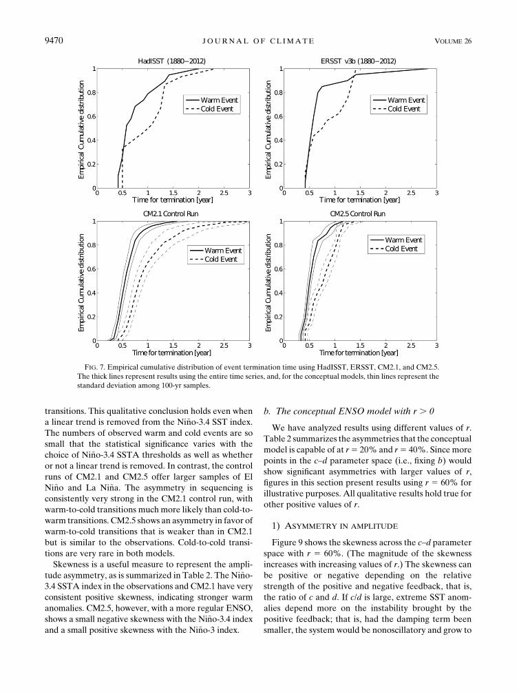
cold events do. Figure 7 shows the cumulative distribu-
tion of termination times for warm and cold events for
the observational datasets and global-climate-model
control run outputs. This result is consistent with
LH2002 andOkumura andDeser (2010). If the Ni~no-3.4
SSTA time series is detrended, cold events appear to last
much longer; that is, the asymmetry in duration is am-
plified upon detrending.
Following the procedures described in section 3,
conditional probabilities for different transition types
are calculated and shown in Fig. 8. From the observa-
tions, there is a higher likelihood to havewarm events be
followed by cold events than vice versa. Cold-to-cold
transitions are also more frequent than warm-to-warm
FIG. 5. Winter years of warm and cold events identified using the percentiles criteria on
HadISST (solid line) and ERSSTv3b (dashed line) datasets. Numbers above (below) the time
series indicate the years when warm (cold) events peak.
FIG. 6. A sample SST anomaly time series, filtered by 5-month running mean, illustrates how
terminations, durations, and transitions are defined. The segment is simulated using the con-
ceptual model with b 5 0.24 month21, c 5 0.49 month21, d 5 0.26 month21, r 5 0.6, � 50.07K22month21, and s 5 0.08g 3 7K ’ 0.01Nm22 if g 5 0.02Nm22K21. Filled circles
indicate event peaks followed by an event of the opposite sign. Crosses indicate event peaks
that are not followed by an event, under the criteria described in section 3.
1 DECEMBER 2013 CHO I ET AL . 9469
transitions. This qualitative conclusion holds even when
a linear trend is removed from the Ni~no-3.4 SST index.
The numbers of observed warm and cold events are so
small that the statistical significance varies with the
choice of Ni~no-3.4 SSTA thresholds as well as whether
or not a linear trend is removed. In contrast, the control
runs of CM2.1 and CM2.5 offer larger samples of El
Ni~no and La Ni~na. The asymmetry in sequencing is
consistently very strong in the CM2.1 control run, with
warm-to-cold transitions much more likely than cold-to-
warm transitions. CM2.5 shows an asymmetry in favor of
warm-to-cold transitions that is weaker than in CM2.1
but is similar to the observations. Cold-to-cold transi-
tions are very rare in both models.
Skewness is a useful measure to represent the ampli-
tude asymmetry, as is summarized in Table 2. The Ni~no-
3.4 SSTA index in the observations and CM2.1 have very
consistent positive skewness, indicating stronger warm
anomalies. CM2.5, however, with a more regular ENSO,
shows a small negative skewness with the Ni~no-3.4 index
and a small positive skewness with the Ni~no-3 index.
b. The conceptual ENSO model with r . 0
We have analyzed results using different values of r.
Table 2 summarizes the asymmetries that the conceptual
model is capable of at r5 20% and r5 40%. Since more
points in the c–d parameter space (i.e., fixing b) would
show significant asymmetries with larger values of r,
figures in this section present results using r 5 60% for
illustrative purposes. All qualitative results hold true for
other positive values of r.
1) ASYMMETRY IN AMPLITUDE
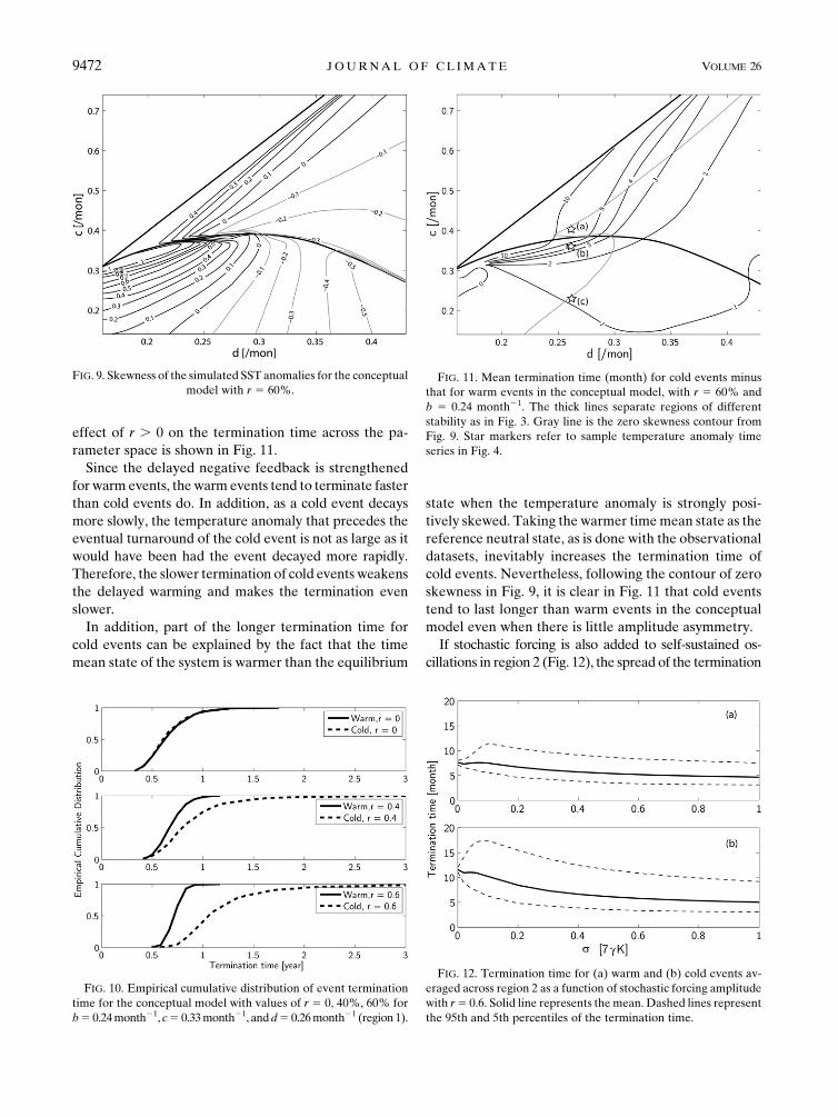
Figure 9 shows the skewness across the c–d parameter
space with r 5 60%. (The magnitude of the skewness
increases with increasing values of r.) The skewness can
be positive or negative depending on the relative
strength of the positive and negative feedback, that is,
the ratio of c and d. If c/d is large, extreme SST anom-
alies depend more on the instability brought by the
positive feedback; that is, had the damping term been
smaller, the system would be nonoscillatory and grow to
FIG. 7. Empirical cumulative distribution of event termination time using HadISST, ERSST, CM2.1, and CM2.5.
The thick lines represent results using the entire time series, and, for the conceptual models, thin lines represent the
standard deviation among 100-yr samples.
9470 JOURNAL OF CL IMATE VOLUME 26

infinity owing to the strong positive feedback. In this case,
positive feedback is enhanced with a larger coupling ef-
ficiency during warm events. Therefore, warm events are
able to grow to larger amplitudes while cold events be-
come relatively weak, resulting in a positive skewness.
Instead, if d/c is large, extreme SST anomalies depend
more on the strong overshooting of the preceding events
of the opposite sign; that is, the system would be oscil-
latory unstable if the damping term was not strong
enough. Therefore, cold events can grow to larger am-
plitudes owing to the stronger delayed cooling of the
preceding warm events, while warm event peaks cannot
grow as much since the delayed warming owing to the
preceding cold events is diminished. In short, if the cou-
pling efficiency is larger during warm events, skewness
becomes positive in the parameter region where positive
feedback strength is large or negative where negative
feedback strength is large. Notice that the cutoff does not
lie along c 5 d because b is nonzero.
2) ASYMMETRY IN DURATION
As r increases, cold events terminate at a later time
than warm events do. This difference in termination
times resembles the behavior found in the observations
and GCMs. Figure 10 shows how the distributions of
event termination time change with the value of r. The
FIG. 8. Conditional probability of transitions for warm and cold events using the Ni~no-3.4 index.
TABLE 2. Parameters that produce the best simulations of observed, CM2.1, andCM2.5 asymmetry statistics. Parameter b is fixed at 0.24
month21, and r is also fixed at values based on the zonal wind stress analysis. Observations are Std: standard deviation of the temperature
anomaly (K), Skewness: skewness of the temperature anomaly, LenDiff: termination time of cold events minus that of warm events (in
months), and Pdiff: probability of warm-to-cold transitionsminus that of cold-to-warm transitions. The row(s) below best fit correspond to
the asymmetry statistics derived from theNi~no-3.4 SSTA index. Parentheses represent statistics computed from the first and second halves
of the Ni~no-3.4 SSTA index time series.
Observations
r Std Skewness LenDiff Pdiff b c d
Best fit 0.2 0.7 0.26 0.52 0.43 0.24 0.37 0.24
HadISST 0.72 (0.68, 0.75) 0.34 (0.26, 0.43) 0.9 (20.4, 2.9) 0.15 (0, 0.2)
ERSST 0.77 (0.72, 0.79) 0.38 (0.35, 0.38) 2.1 (21.1, 4.0) 0.11 (20.1, 0.3)
CM2.1
Best fit 0.4 1.0 0.28 1.9 0.6 0.24 0.36 0.25
Ni~no-3.4 1.2 (0.28, 0.34) (3.3, 3.4) 0.6
CM2.5
Best fit 0.2 1.1 20.13 0.4 0.05 0.24 0.28 0.31
Ni~no-3.4 1.1 (20.16, 20.06) (2.2, 2.8) 0.11 (0.08, 0.12)
1 DECEMBER 2013 CHO I ET AL . 9471
effect of r . 0 on the termination time across the pa-
rameter space is shown in Fig. 11.
Since the delayed negative feedback is strengthened
for warm events, thewarm events tend to terminate faster
than cold events do. In addition, as a cold event decays
more slowly, the temperature anomaly that precedes the
eventual turnaround of the cold event is not as large as it
would have been had the event decayed more rapidly.
Therefore, the slower termination of cold events weakens
the delayed warming and makes the termination even
slower.
In addition, part of the longer termination time for
cold events can be explained by the fact that the time
mean state of the system is warmer than the equilibrium
state when the temperature anomaly is strongly posi-
tively skewed. Taking the warmer timemean state as the
reference neutral state, as is done with the observational
datasets, inevitably increases the termination time of
cold events. Nevertheless, following the contour of zero
skewness in Fig. 9, it is clear in Fig. 11 that cold events
tend to last longer than warm events in the conceptual
model even when there is little amplitude asymmetry.
If stochastic forcing is also added to self-sustained os-
cillations in region 2 (Fig. 12), the spread of the termination
FIG. 9. Skewness of the simulated SST anomalies for the conceptual
model with r 5 60%.
FIG. 10. Empirical cumulative distribution of event termination
time for the conceptual model with values of r 5 0, 40%, 60% for
b5 0.24month21, c5 0.33month21, andd5 0.26month21 (region 1).
FIG. 11. Mean termination time (month) for cold events minus
that for warm events in the conceptual model, with r 5 60% and
b 5 0.24 month21. The thick lines separate regions of different
stability as in Fig. 3. Gray line is the zero skewness contour from
Fig. 9. Star markers refer to sample temperature anomaly time
series in Fig. 4.
FIG. 12. Termination time for (a) warm and (b) cold events av-
eraged across region 2 as a function of stochastic forcing amplitude
with r5 0.6. Solid line represents the mean. Dashed lines represent
the 95th and 5th percentiles of the termination time.
9472 JOURNAL OF CL IMATE VOLUME 26

time distribution for cold events increases more than
that for warm events. When the stochastic forcing in-
tensity is moderate, high percentiles (e.g., 95th) of the
cold event termination time extend more to longer du-
rations than those of the warm events do. As stochastic
forcing continues to amplify, the entire distribution of the
termination time moves to shorter time scales because
the signal begins to be dominated by stochastic forcing,
which has higher frequencies than the ENSO. This result
clearly illustrates the susceptibility of cold events to ex-
ternal forcing.
3) ASYMMETRY IN SEQUENCING
The conceptual model also shows a higher tendency
for warm-to-cold transitions than cold-to-warm transi-
tions with r . 0. As shown in Fig. 13, the probability of
warm-to-cold transitions minus that of cold-to-warm
transitions are positive everywhere in the stable and
stochastically driven region (region 1). In region 2, the
oscillation is self-sustained and is very regular. The
positive difference in the transition probabilities in re-
gion 2, as shown in Fig. 13, is because some of the warm
events peak later than 12 months after the preceding
cold event termination and do not fulfill the transition
criterion (see section 3).
If stochastic forcing is added to region 2, the proba-
bilities of warm-to-warm and cold-to-cold transitions
increase, and the latter increases more than the former,
albeit to a slight extent (Fig. 14).
With the delayed negative feedback being stronger
following warm events and weaker following cold events,
warm events are more likely to be plunged into cold
events than vice versa—since the cooling following warm
events is strong enough to overshoot and is more re-
silient to disruptive stochastic forcing. In contrast, the
weakened delayed warming during the termination of
a cold event lowers the probability of a cold-to-warm
transition. This explains why a stable, stochastically
driven parameter region is necessary for the asymmetry
in sequencing to be revealed in this conceptual model.
5. Summary and discussion
The asymmetries of ENSO were examined using ob-
servational records, coupled climate models, and a simpli-
fied dynamical framework. Three asymmetries between
El Ni~no and La Ni~na are identified in models and obser-
vations: duration, sequencing, and amplitude. The dura-
tion asymmetry is the tendency of cold events to last longer
than warm events do. The amplitude asymmetry involves
warm events tending to be stronger. The sequencing
asymmetry involves the tendency of warm events to be
followed by cold events more readily than vice versa.
The central equatorial Pacific wind stress anomalies also
exhibit an asymmetric response to sea surface temper-
ature anomalies in models and observations. Using the
well-known delayed-oscillator conceptual model, we
parameterize the impact of the zonal wind stress asym-
metric response and demonstrate that this can lead to
the aforementioned asymmetries in a consistent way.
The duration asymmetry is pervasive across the pa-
rameter space that we have explored. The sequencing
asymmetry can be obtained only if there is stochastic
external forcing. The amplitude asymmetry has the
same sign as that observed when the positive feedback
is strong compared to the delayed negative feedback.
FIG. 13. Conditional probability of warm-to-cold transition mi-
nus that of cold-to-warm transitions for r 5 60% across the c–d
parameter space.
FIG. 14. Changes in transition probabilities with increasing
stochastic forcing intensity and fixed r 5 60% for region 2 (self-
sustained oscillations). Results are averaged within the region that
have probability(warm to cold) 5 probability(cold to warm) 5 1
when stochastic forcing is absent.
1 DECEMBER 2013 CHO I ET AL . 9473
The asymmetries owing to the additional nonlinearity
to the ENSO conceptual model can be understood as
follows: warm events are able to grow into larger am-
plitudes with the strengthened positive feedback. When
they decay, the strengthened delayed negative feedback
causes warm events to terminate faster and increases the
chance of a following cold event. The initial growth of
the cold events comes from the preceding warm event,
but the cooling subsides soon after onset. If the over-
shooting is not too strong, the weakened positive feed-
back of cold events causes the cold events to mature at
weaker amplitudes. When cold events terminate, the
delayed negative feedback is weaker. The slower neu-
tralization and the warmer long-term mean state are
responsible for the longer durations of the cold events.
Cold events are also more prone to be disrupted by ex-
ternal forcing and are less likely to be followed by
a warm event. As a result, when there is a warm event,
the predictability of a following cold event is higher.
What follows a cold event is more uncertain. This result
is consistent with Dommenget et al. (2013) that El Ni~nos
are mostly triggered by wind and are less predictable,
while La Ni~nas are more predictable.
The conceptual model simplifies the system into a few
feedback terms and provides a potential guide for in-
vestigations when a climate model simulates ENSO
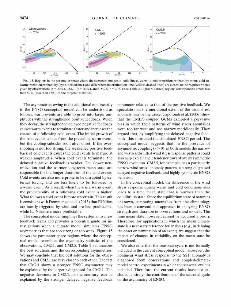
asymmetries that are too strong or too weak. Figure 15
shows the parameter space regions where the concep-
tual model resembles the asymmetry statistics of the
observations, CM2.1, and CM2.5. Table 2 summarizes
the best solutions and the corresponding asymmetries.
We may conclude that the best solutions for the obser-
vations and CM2.1 are very close to each other. The fact
that CM2.1 shows a stronger ENSO asymmetry may
be explained by the larger r diagnosed for CM2.1. The
negative skewness in CM2.5, on the contrary, can be
explained by the stronger delayed negative feedback
parameter relative to that of the positive feedback. We
speculate that the meridional extent of the wind stress
anomaly may be the cause. Capotondi et al. (2006) show
that the CMIP3 coupled GCMs exhibited a pervasive
bias in which their patterns of wind stress anomalies
were too far west and too narrow meridionally. They
argued that, by amplifying the delayed negative feed-
back, this shortened the simulated ENSO period. The
conceptual model suggests that, in the presence of
asymmetric coupling (r. 0), in bothmodels the narrow
and westward-shifted wind stress response patterns could
also help explain their tendency toward overly symmetric
ENSO evolution. CM2.5, for example, has a particularly
narrow wind stress anomaly pattern, a strong diagnosed
delayed negative feedback, and highly symmetric ENSO
behavior.
In the conceptual model, the difference in the wind
stress response during warm and cold conditions also
leads to a time mean state that is warmer than the
equilibrium state. Since the equilibrium state of nature is
unknown, computing anomalies from the climatology
has been a conventional approach in analyzing ENSO
strength and duration in observations and models. The
time mean state, however, cannot be acquired a priori.
Therefore, for applications in which the mean climate
state is a necessary reference for analysis (e.g., in defining
the onset or termination of an event), we suggest that the
impact of changes in variability on the mean state be
considered.
We also note that the seasonal cycle is not formally
included in the current conceptual model. However, the
nonlinear wind stress response to the SST anomaly is
diagnosed from observations and coupled-climate-
model control experiments in which the seasonal cycle is
included. Therefore, the current results have not ex-
cluded, entirely, the contributions of the seasonal cycle
on the asymmetry of ENSO.
FIG. 15. Regions in the parameter space where the skewness (magenta, solid lines), warm-to-cold transition probability minus cold-to-
warm transition probability (cyan, dotted line), and differences in termination time (yellow, dashed lines) are closest to the required values
given by observations (r5 20%), CM2.1 (r5 40%), and CM2.5 (r5 20%); see Table 2. Lighter (darker) regions correspond to errors less
than 50% (less than 15%) of the targeted statistics.
9474 JOURNAL OF CL IMATE VOLUME 26

The coupling efficiency dependence on the polarity of
ENSO could have several causes. For example, obser-
vations indicate that westerly wind burst (WWB) oc-
currence depends on the state of ENSO (Harrison and
Vecchi 1997; Vecchi and Harrison 2000). The state de-
pendence of WWBs, their skewness, and their more
frequent/strong occurrence at the onset of warm events
would potentially be one of the processes that leads to
a positive r, for example, through the low frequency
component of the WWBs. GCM experiments also in-
dicate that the frequency and intensity of WWB can be
promoted during El Ni~no owing to a shifted location of
the warmest water (Lengaigne et al. 2003). Eisenman
et al. (2005) suggest that this state dependence may be
equivalent to an increase in the air–sea coupling strength
during El Ni~no events, andGebbie et al. (2007) show that
adding a state-dependent WWB parameterization to a
hybrid coupled GCM increases the instability, irregu-
larity, and asymmetry of its ENSO simulation.
The observational data for the wind stress responses
suggests r 5 20% for the conceptual model. While the
model at r 5 20% is capable of producing realistic
asymmetries in amplitude and transition probability, the
duration asymmetry is weaker than observed. This sug-
gests that other sources of nonlinearities, such as nonlinear
dynamical heating, the nonlinear relationship between the
eastern Pacific thermocline depth and SST, and the non-
linear rectification of tropical instability waves, are also
important in the understanding of the asymmetries.
The current study raises a number of questions: why is
the wind stress response sensitivity stronger during warm
events? Nonlinearities in atmospheric convection are
a likely source. How important are atmospheric non-
linearities compared to oceanic nonlinearities? What are
the roles of seasonality, ocean adjustment times, and the
spatio-temporal patterns of wind stress coupling in the
conceptual framework described here? How will future
climate changes affect ENSO asymmetries? We are in-
terested in answering these questions in the future.
Acknowledgments. We are indebted to Xiaosong
Yang and Isaac Held for providing comments and sug-
gestions. This report was prepared by KC under Award
NA08OAR4320752 from the National Oceanic and
Atmospheric Administration and U.S. Department of Com-
merce. The statements, findings, conclusions, and recom-
mendations are those of the author(s) and do not necessarily
reflect the views of theNationalOceanic andAtmospheric
Administration or the U.S. Department of Commerce.
REFERENCES
An, S.-I., and F.-F. Jin, 2004: Nonlinearity and asymmetry of
ENSO. J. Climate, 17, 2399–2412.
Battisti, D. S., and A. C. Hirst, 1989: Interannual variability in a
tropical atmosphere–ocean model: Influence of the basic state,
ocean geometry and nonlinearity. J. Atmos. Sci., 46, 1687–1712.
Bjerknes, J., 1969: Atmospheric teleconnections from the equato-
rial Pacific. Mon. Wea. Rev., 97, 163–172.
Bourassa,M.A., R. Romero, S. R. Smith, and J. J. O’Brien, 2005:A
new FSU winds climatology. J. Climate, 18, 3686–3698.Burgers, G., andD. B. Stephenson, 1999: The normality of El Ni~no.
Geophys. Res. Lett., 26, 1027–1030.
Capotondi, A., A. Wittenberg, and S. Masina, 2006: Spatial and
temporal structure of tropical Pacific interannual variability in
20th century coupled simulations.OceanModell., 15, 274–298.
Dee, D. P., and S. Uppala, 2009: Variational bias correction of
satellite radiance data in the ERA-Interim reanalysis. Quart.
J. Roy. Meteor. Soc., 135, 1830–1841.Delworth, T. L., and Coauthors, 2006: GFDL’s CM2 global cou-
pled climate models. Part I: Formulation and simulation
characteristics. J. Climate, 19, 643–674.
——, and Coauthors, 2012: Simulated climate and climate change
in the GFDL CM2.5 high-resolution coupled climate model.
J. Climate, 25, 2755–2781.Dommenget, D., T. Bayr, and C. Frauen, 2013: Analysis of the non-
linearity in the pattern and time evolution of El Ni~no Southern
Oscillation. Climate Dyn., 40, 2825–2847.
Eisenman, I., L. Yu, and E. Tziperman, 2005:Westerly wind bursts:
ENSO’s tail rather than the dog? J. Climate, 18, 5224–5238.
Frauen, C., and D. Dommenget, 2010: El Ni~no and La Ni~na am-
plitude asymmetry caused by atmospheric feedbacks. Geo-
phys. Res. Lett., 37, L18801, doi:10.1029/2010GL044444.
Galanti, E., and E. Tziperman, 2000: ENSO’s phase locking to the
seasonal cycle in the fast-SST, fast-wave, and mixed-mode
regimes. J. Atmos. Sci., 57, 2936–2950.
——,——,M. Harrison, A. Rosati, R. Giering, and Z. Sirkes, 2002:
The equatorial thermocline outcropping—A seasonal control
on the tropical Pacific ocean–atmosphere instability strength.
J. Climate, 15, 2721–2739.Gebbie, G., I. Eisenman, A. Wittenberg, and E. Tziperman, 2007:
Modulation of westerly wind bursts by sea surface tempera-
ture: A semistochastic feedback for ENSO. J. Atmos. Sci., 64,
3281–3295.
Harrison, D. E., and B. S. Giese, 1988: Remote westerly wind
forcing of the eastern equatorial Pacific; some model results.
Geophys. Res. Lett., 15, 804–807.
——, and G. A. Vecchi, 1997: Westerly wind events in the tropical
Pacific, 1986–95. J. Climate, 10, 3131–3156.——, and——, 1999: On the termination of El Ni~no.Geophys. Res.
Lett., 26, 1593–1596.
Hoerling, M. P., A. Kumar, andM. Zhong, 1997: El Ni~no, La Ni~na,
and the nonlinearity of their teleconnections. J. Climate, 10,
1769–1786.
Jin, F.-F., 1997: An equatorial ocean recharge paradigm for ENSO.
Part I: Conceptual model. J. Atmos. Sci., 54, 811–829.
——, S.-I. An, A. Timmermann, and J. Zhao, 2003: Strong El Ni~no
events and nonlinear dynamical heating. Geophys. Res. Lett.,
30, 1120, doi:10.1029/2002GL016356.
Kalnay, E., and Coauthors, 1996: The NCEP/NCAR 40-Year Re-
analysis Project. Bull. Amer. Meteor. Soc., 77, 437–471.Kang, I.-S., and J.-S. Kug, 2002: El Ni~no and La Ni~na sea surface
temperature anomalies: Asymmetry characteristics associated
with their wind stress anomalies. J. Geophys. Res., 107, 4372,
doi:10.1029/2001JD000393.
Kessler, W. S., 2002: Is ENSO a cycle or a series of events? Geo-
phys. Res. Lett., 29, 2125, doi:10.1029/2002GL015924.
1 DECEMBER 2013 CHO I ET AL . 9475
Kistler, R., and Coauthors, 2001: The NCEP–NCAR 50-Year
Reanalysis: Monthly means CD-ROM and documentation.
Bull. Amer. Meteor. Soc., 82, 247–267.
Larkin, N.K., andD. E.Harrison, 2002: ENSOwarm (ElNi~no) andcold (La Ni~na) event life cycles: Ocean surface anomaly pat-
terns, their symmetries, asymmetries, and implications.
J. Climate, 15, 1118–1140.
Lengaigne,M., J.-P. Boulanger, C.Menkes, G.Madec, P. Delecluse,
E. Guilyardi, and J. Slingo, 2003: The March 1997 westerly
wind event and the onset of the 1997/98 El Ni~no: Under-
standing the role of the atmospheric response. J. Climate, 16,
3330–3343.
Okumura,Y.M., andC.Deser, 2010: Asymmetry in the duration of
El Ni~no and La Ni~na. J. Climate, 23, 5826–5843.
——, M. Ohba, C. Deser, and H. Ueda, 2011: A proposed mech-
anism for the asymmetric duration of El Ni~no and La Ni~na.
J. Climate, 24, 3822–3829.
Philip, S., and G. J. van Oldenborgh, 2009: Significant atmospheric
nonlinearities in the ENSO cycle. J. Climate, 22, 4014–4028.Picaut, J., F. Masia, and Y. D. Penhoat, 1997: An advective-
reflective conceptual model for the oscillatory nature of the
ENSO. Science, 277, 663–666.
Rayner, N. A., D. E. Parker, E. B. Horton, C. K. Folland, L. V.
Alexander, D. P. Rowell, E. C. Kent, and A. Kaplan, 2003:
Global analyses of sea surface temperature, sea ice, and night
marine air temperature since the late nineteenth century.
J. Geophys. Res., 108, 4407, doi:10.1029/2002JD002670.
Rienecker, M. M., and Coauthors, 2011: MERRA: NASA’s
Modern-Era Retrospective Analysis for Research and Ap-
plications. J. Climate, 24, 3624–3648.Smith, T. M., R. W. Reynolds, T. C. Peterson, and J. Lawrimore,
2008: Improvements to NOAA’s historical merged land–
ocean surface temperature analysis (1880–2006). J. Climate,
21, 2283–2296.Suarez,M. J., and P. S. Schopf, 1988: A delayed action oscillator for
ENSO. J. Atmos. Sci., 45, 3283–3287.
Tziperman, E., S. E. Zebiak, andM. A. Cane, 1997: Mechanisms of
seasonal–ENSO interaction. J. Atmos. Sci., 54, 61–71.
Uppala, S. M., and Coauthors, 2005: The ERA-40 Re-Analysis.
Quart. J. Roy. Meteor. Soc., 131, 2961–3012.
Vecchi, G.A., 2006: The termination of the 1997–98 ElNi~no. Part II:
Mechanisms of atmospheric change. J. Climate, 19, 2647–2664.——, and D. E. Harrison, 2000: Tropical Pacific sea surface tem-
perature anomalies, El Ni~no, and equatorial westerly wind
events. J. Climate, 13, 1814–1830.
——, and——, 2006: The termination of the 1997–98 El Ni~no. Part I:Mechanisms of oceanic change. J. Climate, 19, 2633–2646.
——, and A. T. Wittenberg, 2010: El Ni~no and our future climate:
Where do we stand? Wiley Interdiscip. Rev.: Climate Change,
1, 260–270.——, A. Clement, and B. J. Soden, 2008: Examining the tropical
Pacific’s response to global warming.Eos, Trans. Amer.Geophys.
Union, 89, 81–83.Vialard, J., C. Menkes, J.-P. Boulanger, P. Delecluse, E. Guilyardi,
M. J. McPhaden, and G. Madec, 2001: Amodel study of oceanic
mechanisms affecting equatorial Pacific sea surface temperature
during the 1997–98 El Ni~no. J. Phys. Oceanogr., 31, 1649–1675.Wang, W., and M. J. McPhaden, 2000: The surface-layer heat
balance in the equatorial Pacific Ocean. Part II: Interannual
variability. J. Phys. Oceanogr., 30, 2989–3008.
Weisberg, R. H., and C. Wang, 1997: A western Pacific oscillator
paradigm for the El Ni~no-Southern Oscillation.Geophys. Res.
Lett., 24, 779–782.
Wittenberg, A. T., 2004: Extended wind stress analyses for ENSO.
J. Climate, 17, 2526–2540.
——, 2009: Are historical records sufficient to constrain ENSO
simulations? Geophys. Res. Lett., 36, L12702, doi:10.1029/
2009GL038710.
——, A. Rosati, N.-C. Lau, and J. J. Ploshay, 2006: GFDL’s CM2
global coupled climate models. Part III: Tropical Pacific cli-
mate and ENSO. J. Climate, 19, 698–722.
Wolter, K., and M. S. Timlin, 2011: El Ni~no/Southern Oscillation
behaviour since 1871 as diagnosed in an extendedmultivariate
ENSO index (MEI.ext). Int. J. Climatol., 31, 1074–1087.
Zebiak, S. E., and M. A. Cane, 1987: A model El Ni~no–SouthernOscillation. Mon. Wea. Rev., 115, 2262–2278.
9476 JOURNAL OF CL IMATE VOLUME 26