The Pennsylvania State University
The Graduate School
The Smeal College of Business
EMPIRICAL MODELS FOR ORGANIZATIONAL SERVICE
QUALITY DECISIONS
A Dissertation in
Business Administration
by
Chen Zhou
c⃝ 2013 Chen Zhou
Submitted in Partial Fulllmentof the Requirementsfor the Degree of
Doctor of Philosophy
August 2013

The dissertation of Chen Zhou was reviewed and approved* by the following:
Rajdeep GrewalIrving & Irene Bard Professor of MarketingDissertation AdvisorChair of Committee
Gary LilienDistinguished Research Professor of Management Science
Min DingSmeal Professor of Marketing and InnovationSpecial Signatory
Alok KumarAssistant Professor of Marketing
Paulo AlbuquerqueAssociate Professor of MarketingSimon School of Business, University of RochesterSpecial Member
Mark RobertsProfessor of EconomicsDepartment of Economics, Penn State University
Duncan K. H. FongProfessor of Marketing and Professor of StatisticsHead of the Department of Marketing
*Signatures are on le in the Graduate School.
ii

Abstract
In my dissertation, I explore how service quality decisions of rms are inuenced by fac-
tors such as pricing decisions, market and rm characteristics, and competition. In essay I, I
study the joint dynamic decisions of service quality and price. I also explicitly recognize that
rms make service quality and pricing decisions in the presence of competitive forces (e.g.,
Steenkamp, Nijs, Hanssens and Dekimpe, 2005). Thus, I develop a model to capture the dy-
namic interplay among service quality (represented by ight delays), price, and performance
outcomes (i.e., capacity utilization and demand) in the presence of potential competition
(i.e., number of competitors, e.g., Mazzeo, 2003) and realized competition (i.e., actual com-
petitive actions, e.g., Chandrashekaran, Mehta, Chandrashekaran and Grewal, 1999) for
services rm. With the U.S. airline industry as the research context, I collect market (route)
level, quarterly data from major rms (airlines) in those markets, and propose a structural
vector autoregressive panel model. The results suggest interesting patterns of the asymmetry
between service quality and price. In particular, though service quality decisions adjust to
pricing decisions, pricing decisions are not adjusted to service quality decisions. Together
with the result for competition variables, this nding indicates that rms adjust their prices
primarily to manage capacity and in response to potential and realized competition. Ser-
vice quality decisions instead reect considerations of price, performance, and competitive
factors. In essay II, I take a step further to explore how rms' service quality decisions are
inuenced by competitors' service quality decisions, market characteristics (i.e., potential
demand), and rm characteristics (i.e., market power). I use both ight cancellations and
ight delays as indicators of service quality. I apply the static game estimation method to
correct for potential estimation bias from the endogeneity of competitors' service decisions.
The results suggest that ight cancellation and delay decisions are asymmetrically inuenced
by rm characteristics and competition. Specically, ight cancellation decisions tend to be
driven by rm characteristics related to cancellation costs and rescheduling convenience,
while ight delay decisions are responsive to competition; in particular, rms tend to adjust
their ight delay levels to dierentiate their services from those of their competitors.
iii

Contents
List of Figures vi
List of Tables vii
Acknowledgments viii
1 Introduction 1
2 Modeling Service Quality, Price, and Performance at the Market Level:
The Role of Potential and Realized Competition 4
2.1 Introduction . . . . . . . . . . . . . . . . . . . . . . . . . . . . . . . . . . . . . . 52.2 Research Context and Data . . . . . . . . . . . . . . . . . . . . . . . . . . . . . 7
2.2.1 Research Setting . . . . . . . . . . . . . . . . . . . . . . . . . . . . . . . 72.2.2 Data Structure and Measures . . . . . . . . . . . . . . . . . . . . . . . 8
2.2.2.1 Competition . . . . . . . . . . . . . . . . . . . . . . . . . . . 112.2.2.2 Control Variables . . . . . . . . . . . . . . . . . . . . . . . . 122.2.2.3 Missing Data . . . . . . . . . . . . . . . . . . . . . . . . . . . 13
2.2.3 Descriptive Analysis . . . . . . . . . . . . . . . . . . . . . . . . . . . . . 132.3 Model Specication . . . . . . . . . . . . . . . . . . . . . . . . . . . . . . . . . 17
2.3.1 Three-Way Data . . . . . . . . . . . . . . . . . . . . . . . . . . . . . . . 182.4 VAR Specication . . . . . . . . . . . . . . . . . . . . . . . . . . . . . . . . . . . 19
2.4.1 Panel VAR Model . . . . . . . . . . . . . . . . . . . . . . . . . . . . . . 212.4.2 Cross-Sectional Dependence . . . . . . . . . . . . . . . . . . . . . . . . 222.4.3 Missing Data . . . . . . . . . . . . . . . . . . . . . . . . . . . . . . . . . 23
2.5 Model Estimation . . . . . . . . . . . . . . . . . . . . . . . . . . . . . . . . . . . 252.5.1 Unit Root Tests . . . . . . . . . . . . . . . . . . . . . . . . . . . . . . . 252.5.2 Number of Lags . . . . . . . . . . . . . . . . . . . . . . . . . . . . . . . . 262.5.3 Missing Data . . . . . . . . . . . . . . . . . . . . . . . . . . . . . . . . . 262.5.4 Unobserved Heterogeneity . . . . . . . . . . . . . . . . . . . . . . . . . 272.5.5 Cross-Sectional Dependence . . . . . . . . . . . . . . . . . . . . . . . . 28
2.5.5.1 Stage 1: Instrumental variable regression to each equationin the VAR system . . . . . . . . . . . . . . . . . . . . . . . . 29
2.5.5.2 Stage 2: Estimate ρ . . . . . . . . . . . . . . . . . . . . . . . 302.5.5.3 Stage 3: Estimate the PVARX model with ρ . . . . . . . . 30
2.5.6 PVAR Estimation . . . . . . . . . . . . . . . . . . . . . . . . . . . . . . 312.6 Results . . . . . . . . . . . . . . . . . . . . . . . . . . . . . . . . . . . . . . . . . 32
2.6.1 Missing Data . . . . . . . . . . . . . . . . . . . . . . . . . . . . . . . . . 322.6.2 Unit Root Tests . . . . . . . . . . . . . . . . . . . . . . . . . . . . . . . 322.6.3 Number of Lags . . . . . . . . . . . . . . . . . . . . . . . . . . . . . . . 332.6.4 Cross-Sectional Dependence . . . . . . . . . . . . . . . . . . . . . . . . 332.6.5 Panel VAR . . . . . . . . . . . . . . . . . . . . . . . . . . . . . . . . . . 33
iv

2.6.5.1 Impact on Service Quality . . . . . . . . . . . . . . . . . . . 342.6.5.2 Impact on Price . . . . . . . . . . . . . . . . . . . . . . . . . 372.6.5.3 Competitive Eects . . . . . . . . . . . . . . . . . . . . . . . 382.6.5.4 Control Variables . . . . . . . . . . . . . . . . . . . . . . . . 39
2.7 Conclusion . . . . . . . . . . . . . . . . . . . . . . . . . . . . . . . . . . . . . . 40
3 Modeling Service Quality: The Impact of Firm, Demand, and Competitive
Factors 42
3.1 Introduction . . . . . . . . . . . . . . . . . . . . . . . . . . . . . . . . . . . . . . 443.2 Literature Review . . . . . . . . . . . . . . . . . . . . . . . . . . . . . . . . . . . 473.3 Background Information: On-Time Performance in Airline Industry . . . . . 483.4 Data . . . . . . . . . . . . . . . . . . . . . . . . . . . . . . . . . . . . . . . . . . 51
3.4.1 Data Description . . . . . . . . . . . . . . . . . . . . . . . . . . . . . . . 513.4.2 Examples of Service Quality Variation . . . . . . . . . . . . . . . . . . . 523.4.3 Model-Free Evidence of Market, Firm, and Competitive Characteristics 53
3.5 Model . . . . . . . . . . . . . . . . . . . . . . . . . . . . . . . . . . . . . . . . . . 583.5.1 Justication for Assumptions . . . . . . . . . . . . . . . . . . . . . . . . 583.5.2 Intuitions Behind the Model . . . . . . . . . . . . . . . . . . . . . . . . 593.5.3 Formal Specication of the Model . . . . . . . . . . . . . . . . . . . . . 60
3.6 Model Identication and Estimation Method . . . . . . . . . . . . . . . . . . . 633.6.1 Conditions for Identication . . . . . . . . . . . . . . . . . . . . . . . . 633.6.2 Existence and Multiplicity of Equilibria . . . . . . . . . . . . . . . . . . 653.6.3 Endogeneity . . . . . . . . . . . . . . . . . . . . . . . . . . . . . . . . . . 653.6.4 Estimation Method . . . . . . . . . . . . . . . . . . . . . . . . . . . . . . 66
3.7 Results . . . . . . . . . . . . . . . . . . . . . . . . . . . . . . . . . . . . . . . . . 673.7.1 Analysis of Parameter Estimates . . . . . . . . . . . . . . . . . . . . . . 673.7.2 Discussion of Drivers of Service Quality Decisions . . . . . . . . . . . . 703.7.3 Robustness Checks . . . . . . . . . . . . . . . . . . . . . . . . . . . . . . 73
3.7.3.1 Alternative Service Quality Discretization-Trichotomization 743.7.3.2 Continuous Values of Service Quality-Reduced-Form Analysis 89
3.8 Counterfactual Analysis: How New Entrants Drive Incumbents to AdjustService Quality . . . . . . . . . . . . . . . . . . . . . . . . . . . . . . . . . . . . 90
3.9 Discussion and Conclusion . . . . . . . . . . . . . . . . . . . . . . . . . . . . . . 933.9.1 Summary of Key Findings . . . . . . . . . . . . . . . . . . . . . . . . . . 933.9.2 Contribution to the Literature . . . . . . . . . . . . . . . . . . . . . . . 953.9.3 Managerial Implication: Competitors' Service Quality Adjustments on
the Focal Firm's Prots . . . . . . . . . . . . . . . . . . . . . . . . . . . 963.9.4 Research Implications and Future Research . . . . . . . . . . . . . . . . 99
4 Conclusions 100
Bibliography 104
Appendix Supplementary documents 113
v

List of Figures
2.1 Histogram for Minutes of Delay . . . . . . . . . . . . . . . . . . . . . . . . . . . 11
2.2 Time Variation in Service Quality and Price for Select Routes . . . . . . . . . 16
2.3 Impact on Service Quality: Impulse Response Functions . . . . . . . . . . . . 36
2.4 Impact on Price: Impulse Response Functions . . . . . . . . . . . . . . . . . . 37
3.1 Flight On-Time Performances, American Airlines vs. Southwest Airlines . . 46
3.2 Evolution of delay (in minutes), in two markets: Atlanta-San Francisco and
Los Angeles-Denver . . . . . . . . . . . . . . . . . . . . . . . . . . . . . . . . . 53
3.3 Evolution of cancellation rate (in fraction of total ights), in two markets:
Atlanta-San Francisco and Los Angeles-Denver . . . . . . . . . . . . . . . . . 54
3.4 Cancellation rate (fraction of cancelled ights out of total ights) for two groups of
markets, divided by income per capita and the existence of a competitor's hub 55
3.5 Cancellation rate for two group of rms based on rm characteristics: number
of departures performed, capacity utilization, and hub destination. . . . . . . 56
3.6 Incumbents' Service Quality Reaction to Southwest Entry: Origin Boston . . 57
A.1 Time Variation in Logit Delay for Select Routes . . . . . . . . . . . . . . . . . 114
A.2 Time Variation in Log Price for Select Routes . . . . . . . . . . . . . . . . . . 115
A.3 Time Variation in Log Number of Passengers Served for Select Routes . . . . 116
A.4 Time Variation in Logit Capacity Utilization for Select Routes . . . . . . . . . 117
A.5 Impact on Capacity Utilization: Impulse Response Functions . . . . . . . . . 118
A.6 Impact on Number of Passenger Served: Impulse Response Functions . . . . . 119
vi

List of Tables
2.1 List of Variables . . . . . . . . . . . . . . . . . . . . . . . . . . . . . . . . . . . . 9
2.2 Descriptive Statistics and Bivariate Correlation Coecients . . . . . . . . . . 14
2.3 Descriptive Statistics and Bivariate Correlation Coecients (continued) . . . 15
2.4 Cross-Sectional Dependence . . . . . . . . . . . . . . . . . . . . . . . . . . . . . 33
2.5 Panel VAR Results . . . . . . . . . . . . . . . . . . . . . . . . . . . . . . . . . . 35
2.6 Summary of Eects of Endogenous Variables . . . . . . . . . . . . . . . . . . . 36
2.7 Results of Mazzeo Replication . . . . . . . . . . . . . . . . . . . . . . . . . . . . 39
3.1 Descriptive Statistics . . . . . . . . . . . . . . . . . . . . . . . . . . . . . . . . . 58
3.2 Variables that Dene the State Space . . . . . . . . . . . . . . . . . . . . . . . 66
3.3 Parameter Estimates . . . . . . . . . . . . . . . . . . . . . . . . . . . . . . . . . 71
3.4 State Variables and Cancellation Decision . . . . . . . . . . . . . . . . . . . . 72
3.5 State Variables and Delay Decision . . . . . . . . . . . . . . . . . . . . . . . . 74
3.6 Parameter Estimates: Cancellation-33%-67% Threshold . . . . . . . . . . . . 76
3.7 Parameter Estimates: Cancellation-30%-70% Threshold . . . . . . . . . . . . 77
3.8 Parameter Estimates: Delay-33%-67% Threshold . . . . . . . . . . . . . . . . 79
3.9 Parameter Estimates: Delay-30%-70% Threshold . . . . . . . . . . . . . . . . 80
3.10 Parameter Estimates: Cancellation and Delay, 33%-67% Threshold, Part 1 . 84
3.11 Parameter Estimates: Cancellation and Delay, 33%-67% Threshold, Part 2 . 85
3.12 Parameter Estimates: Cancellation and Delay, 30%-70% Threshold, Part 1 . 86
3.13 Parameter Estimates: Cancellation and Delay, 30%-70% Threshold, Part 2 . 87
3.14 Analysis of Competition Eects . . . . . . . . . . . . . . . . . . . . . . . . . . 89
3.15 Results of Seemingly Unrelated Regressions of Cancellation and Delay . . . . 91
3.16 Reaction of UA to Entry of Southwest . . . . . . . . . . . . . . . . . . . . . . . 92
3.17 Reaction of Incumbents to New Entrants: Denver-Minneapolis . . . . . . . . . 94
3.18 Focal Firm's Prots and Competitors' Service Quality Adjustment . . . . . . 98
3.19 Focal Firm's Prots and Competitors' Service Quality Adjustment (converged
results) . . . . . . . . . . . . . . . . . . . . . . . . . . . . . . . . . . . . . . . . . 98
vii

Acknowledgments
I would like to thank my advisor, Rajdeep Grewal, for all his help, support and encourage-
ment as I pursued this long journey of accomplishing the Ph.D. I never would have made this
journey without the support of my committee members, Gary Lilien, Paulo Albuquerque,
Mark Roberts, Min Ding and Alok Kumar. From how to form a good research problem, to
technical details, to how to position and present a research paper, I learned so much from
all of you. Thank my advisor and my committee members for spending time and eort in
helping me grow as a researcher! Through out the past ve years, I also got a lot of support
and encouragement from every faculty member in the marketing department. I would like
to express my appreciation and gratitude to everyone of them.
I am also very lucky to have great peer colleagues in the Ph.D. program in Smeal,
Anindita, Alok, Charles, SungHoon, Li, Aditya, Paolo, Jimmy, Jianing, Yuan, etc.. We
shared joy and pain in the process, and we grow together! I also want to thank my friends
in other schools, Yan, Zhongyao, Xiao, Tian, etc., for your support in both my research and
my daily life. You made my life in State College full of joy!
Through out the process, my mother and other family members constantly provided
needed support and encouragement. Thank you for being so understanding, I love you
all. Last but not least, I would like to thank my best friend, Rafael, for being extremely
understanding and supportive. Thank you for sharing the journey with me!
viii

Chapter 1
Introduction
In the service sector, such as airlines and hotels, it is critical for rms to improve the quality
of their core products - services. Indeed, it is well established in service marketing literature
that emphasis on service quality leads to many positive outcomes, such as increased customer
satisfaction and customer retention rate. (e.g., Lariviere, 2008; Spreng and Mackoy, 1996;
Zeithaml, Berry and Parasuraman, 1996). As service quality is critical for the success of
service rms, it is reasonable to expect that service rms should lay heavy emphasis on service
quality to provide the highest possible level of service quality. However, this conjecture
seems to go against reality. In the airline industry, ight cancellations and delays are not
uncommon. In the hotel industry, being short of sta seems not to be a rare problem. The
inconsistency between what the literature suggests and what rms are actually doing aroused
my interests in understanding how service rms determine their service quality levels, and
what factors drive these decisions. I aim at answering these questions by my two dissertation
essays.
The research topic of understanding rms' service quality decisions is important for en-
riching the services marketing literature and providing managerial implication for services
rms. Despite rich and in-depth research on how service quality drives potential rm perfor-
mance outcomes, there are few studies treating the service quality as the outcome variable.
Some studies discuss how rms may improve service quality by being market oriented (Raju
and Lonial, 2001), formalizing the selling process, and/or applying a cross-functional team
structure (Froehle, Roth, Chase and Voss, 2000). Previous research seems to suggest that
rms should always improve their service quality. However, is it always protable for rms
to improve service quality? Is it possible that some rms strategically choose not to pro-
vide good services under certain market conditions? To answer these questions, we need to
explicitly discuss how rms decide their service quality levels, which previous research has
not explored. I believe this dissertation should contribute to services marketing literature by
1
2
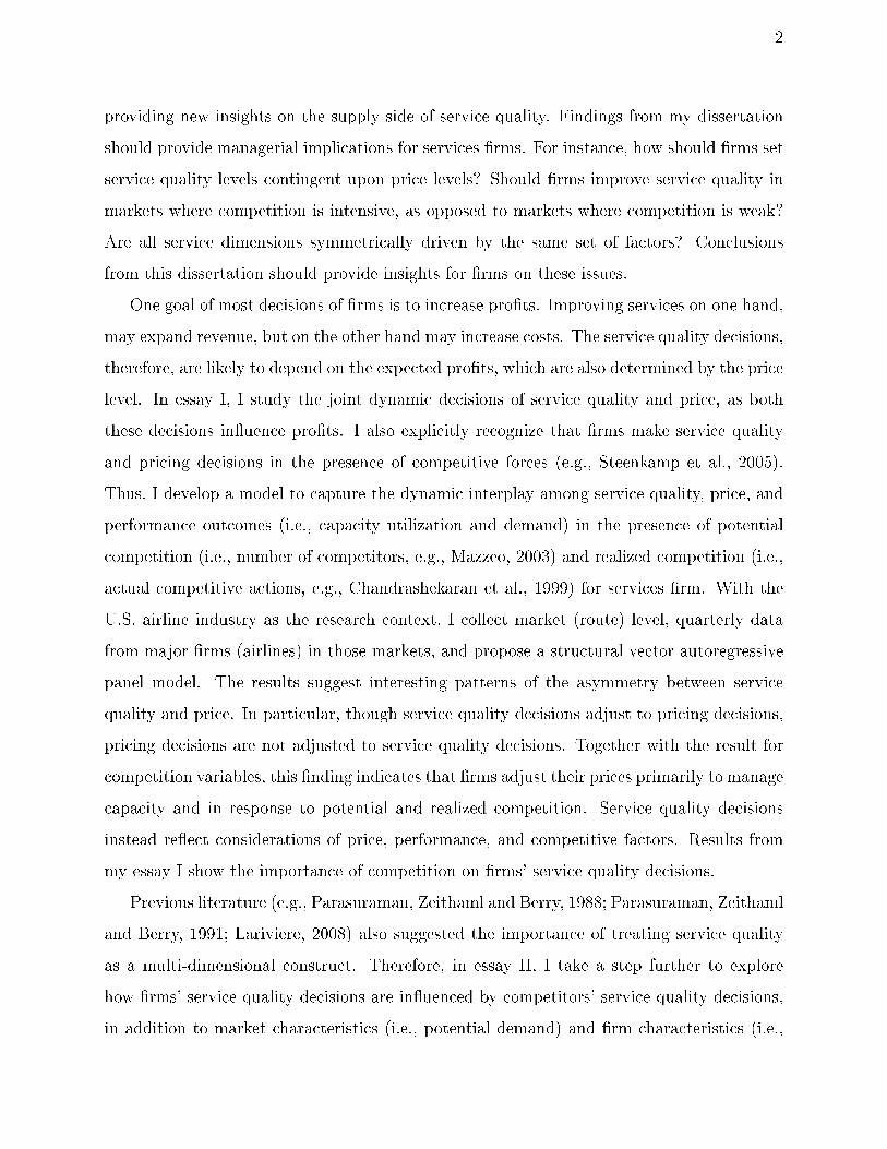
providing new insights on the supply side of service quality. Findings from my dissertation
should provide managerial implications for services rms. For instance, how should rms set
service quality levels contingent upon price levels? Should rms improve service quality in
markets where competition is intensive, as opposed to markets where competition is weak?
Are all service dimensions symmetrically driven by the same set of factors? Conclusions
from this dissertation should provide insights for rms on these issues.
One goal of most decisions of rms is to increase prots. Improving services on one hand,
may expand revenue, but on the other hand may increase costs. The service quality decisions,
therefore, are likely to depend on the expected prots, which are also determined by the price
level. In essay I, I study the joint dynamic decisions of service quality and price, as both
these decisions inuence prots. I also explicitly recognize that rms make service quality
and pricing decisions in the presence of competitive forces (e.g., Steenkamp et al., 2005).
Thus, I develop a model to capture the dynamic interplay among service quality, price, and
performance outcomes (i.e., capacity utilization and demand) in the presence of potential
competition (i.e., number of competitors, e.g., Mazzeo, 2003) and realized competition (i.e.,
actual competitive actions, e.g., Chandrashekaran et al., 1999) for services rm. With the
U.S. airline industry as the research context, I collect market (route) level, quarterly data
from major rms (airlines) in those markets, and propose a structural vector autoregressive
panel model. The results suggest interesting patterns of the asymmetry between service
quality and price. In particular, though service quality decisions adjust to pricing decisions,
pricing decisions are not adjusted to service quality decisions. Together with the result for
competition variables, this nding indicates that rms adjust their prices primarily to manage
capacity and in response to potential and realized competition. Service quality decisions
instead reect considerations of price, performance, and competitive factors. Results from
my essay I show the importance of competition on rms' service quality decisions.
Previous literature (e.g., Parasuraman, Zeithaml and Berry, 1988; Parasuraman, Zeithaml
and Berry, 1991; Lariviere, 2008) also suggested the importance of treating service quality
as a multi-dimensional construct. Therefore, in essay II, I take a step further to explore
how rms' service quality decisions are inuenced by competitors' service quality decisions,
in addition to market characteristics (i.e., potential demand) and rm characteristics (i.e.,

3
market power). I use both percentage of ight cancellations and average ight delays to
represent service quality. Firms may expect each other's service quality decisions and choose
their service levels accordingly. I thus apply the static game estimation method to correct
for the potential estimation bias from the endogeneity of competitors' service decisions as
independent variables. The results suggest that ight cancellation and delay decisions are
asymmetrically inuenced by rm characteristics and competition. Specically, ight can-
cellation decisions tend to be strongly driven by rm characteristics related to cancellation
costs and rescheduling convenience, while ight delay decisions are strongly responsive to
competition; in particular, rms tend to adjust their ight delay levels to either horizontally
or vertically dierentiate their services from those of their competitors.
The ndings of both essays show that there are many factors potentially inuence rms'
service quality decisions: these decisions are made contingent upon other marketing deci-
sions, such as prices; service quality decisions are also constrained by performance outcomes,
such as capacity management and demand; in addition, the service quality decision of a
rm is also inuenced by the intensity of market competition, as well as the competitors'
service performances. Therefore, it is not always feasible or optimal for rms to improve
their services. These ndings contribute to the service marketing literature by introducing
contextual factors to the study of service quality. They also provide references for rms on
how to decide service quality levels.

Chapter 2
Modeling Service Quality, Price, and
Performance at the Market Level: The Role of
Potential and Realized Competition
Abstract
For service rms, service quality and price are the two main strategic tools for ef-
fective competition. To capture the dynamic interplay among service quality, price,
and performance outcomes, this study investigates competitive actions at the market
level, using the U.S. airline industry and quarterly data about airlines competing in
important markets (routes). The model features (1) a three-way data structure with
variables varying across rms (airlines), markets, and time; (2) four endogenous vari-
ables service quality (delays), price, and market-level performance measured by the
number of passengers served and capacity utilization; (3) a vast number of markets
(582 routes) and rms (seven airlines), such that the cross-sections of the data exceed
the time dimensions (maximum 72 quarters); (4) exogenous competition and control
variables; (5) dependence among markets, mainly caused by reciprocal routes; and (6)
missing price information (11.41% of observations). The results of the structural vec-
tor autoregressive panel model oer evidence of cross-sectional dependence. Impulse
response functions for statistical inference suggest that price decisions inuence service
quality decisions and performance outcomes; service quality decisions inuence perfor-
mance outcomes but not price decisions. Finally, service quality increases as realized
competition (competitive action) increases, whereas price increases as either potential
(number of competitors) or realized competition increase.
4

5
2.1. Introduction
Managing service rms in industries such as banking, hospitality, and airlines requires or-
ganizational decisions about the service quality (Mittal, Kamakura and Govind, 2004) and
pricing (Pan, Ratchford and Shankar, 2002) levels that can best acquire and retain customers
(Rust, Danaher and Varki, 2000). These decisions require some consideration of competi-
tors' actions too, such that they vary from one market to another. For example, the service
quality and price oered in hotels depends on their locations and the intensity of competition
in that area (Mazzeo, 2002); similarly, airlines often temporarily reduce fares and increase
service quality on routes (markets) after low-cost carriers enter (Snider, 2009); Walmart's
eect on small retailers in geographically isolated markets also has been well documented
(Ingram, Yue and Rao, 2010). With this article, I seek to develop a model that can cap-
ture the dynamic interplay among service quality, price, and performance outcomes, in the
presence of such competitive actions at the market level.
With this proposition, I assert that the interplay between service quality and price plays
out mainly at the market level. For example, hotels increase service quality and/or lower
prices when the intensity of competition in their market increases (Mazzeo, 2002) and airlines
exhibit similar behaviors in face of new entrants (Shepherd and Brock, 2009); at any given
point in time, the levels of service quality and price vary across markets, together with
the level of competition. The proposed time-series model at the rm and market levels
thus entails a three-way (rmmarkettime) data structure. Furthermore, because service
quality and price might inuence each other, and both variables should be inuenced by
and should inuence performance, I also need a vector autoregressive (VAR) specication in
which service quality, price, and market-level performance are endogenous and inuence each
other (Hamilton, 1994). The possibility that prices can be adjusted easily, in the presence
of lagged eects, means that I also must allow for contemporaneous eects of price, which
requires a structural VAR specication (Cooley and Dwyer, 1998).
Three additional issues also inuence the model development and ability to address the
research question. First, several rms compete in a market, and the number of competitors
varies across markets and over time, such that I encounter a time-series, cross-sectional data

6
structure, for which panel models are appropriate (Baltagi, 2005). Typical panel models
involve a single dependent variable and correct for endogeneity using instrumental variables
(Arellano and Bond, 1991); however, I have multiple dependent variables (service quality,
price, and performance) and thus need a panel structural VAR setup, as has appeared in some
recent literature (Binder, Hsiao and Pesaran, 2005). Second, I recognize that the markets are
interdependent; service quality and pricing decisions are interrelated across markets. Thus,
I also seek to model cross-sectional dependence in the panel VAR framework (Huang, 2008).
Third, to study the role of competition, I must note both potential (number of competitors)
and realized (competitors' actions) competition on service quality and price. Consistent with
extant research (e.g., Steenkamp et al., 2005), I model service quality and price competition as
exogenous, which results in a panel structural VARX model with cross-sectional dependence.
I test the model in the U.S. airline industry, for which both service quality and pricing
decisions are criticalas eectively illustrated by two famous events. In what became popu-
larly known as the Valentine's Day Massacre, Jet Blue stranded nine planes on the tarmac
at JFK Airport for more than six hours during a winter storm on February 14, 2007; this
service failure represented a massive embarrassment for Jet Blue and a critical case study
on service failures (Hoyt, O'Reilly, Rao and Sutton, 2010). In the Mother of all Pricing
Battles in the summer of 1992, the U.S. airlines industry witnessed a brutal price war that,
by some estimates, resulted in $1.53 billion in losses due to fare reductions (Morrison and
Winston, 1996). In this setting, I dene a market as a route from one city to another,
and I collate data from multiple secondary sources to develop a model that can capture
context idiosyncrasies, such as the cross-sectional dependencies that arise from reciprocal
routes (i.e., the route from city A to city B is reciprocal to the route from city B to city A),
as well as unique data challenges (e.g., missing price information). As I detail, the results
from the panel VAR model indicate cross-sectional dependence; price decisions inuence
service quality decisions and performance outcomes, whereas service quality decisions inu-
ence performance outcomes but not price decisions. As we might expect, price is inuenced
positively by both potential and realized competition; however, service quality is negatively
inuenced by potential competition and positively inuenced by realized competition. Con-
sistent with extant research (Mazzeo, 2003; Rupp, Owens and Plumly, 2006), the potential

7
competition nding reverses in the cross-sectional analysis, which suggests the superiority
of this model over cross-sectional models for studying service quality and competition in
multimarket service contexts.
I organize the remainder of this article as follows: I begin by detailing my research context
and data structure, and I provide model-free insights from the data. Next, I develop a model
to capture the requisite elements of the data structure, followed by model estimation details.
After I present the results, I conclude with implications and contributions of this study.
2.2. Research Context and Data
2.2.1 Research Setting
To study the interplay among service quality, price, and performance, I require a context in
which both service quality and price are important decisions and longitudinal data about
these important variables are available. Furthermore, considering my interest in modeling
the eects of potential and realized competition related to service quality and price, rms
should compete on both variables. Finally, to model competitive eects, I must be able to
dene competition at the market level and have access to competition data for both service
quality and price variables.
The airline industry meets these criteria. In this service sector, service quality is impor-
tant and has been widely studied (e.g., Grewal, Chandrashekaran and Citrin, 2010). Pricing
decisions also are critical for the success of airlines (Busse, 2002). Airlines compete in distinct
markets (i.e., routes between cities; Snider 2009), so I can identify airlines that compete in
each market and determine competition on both service quality (Mazzeo, 2003) and pricing
(Gerardi and Shapiro, 2009). Overall, the airline industry is an appropriate context in which
to model competitive interactions of service quality and pricing.
Currently the Airline Deregulation Act of 1978, which replaced the Civil Aeronautics Act
of 1938, governs the U.S. airlines industry. The Airline Deregulation Act aims to encour-
age, develop, and maintain air transportation system by relaying on actual and potential
competition to provide eciency, innovation, and low prices, and to determine the variety,
8
quality, and price of air transportation services (Shepherd and Brock, 2009, p. 238). This
quote from Shepherd and Brock (2009) uses language directly from the Airline Deregulation
Act of 1978 and establishes the importance of price, service quality, and competition that
from the crux of this research.
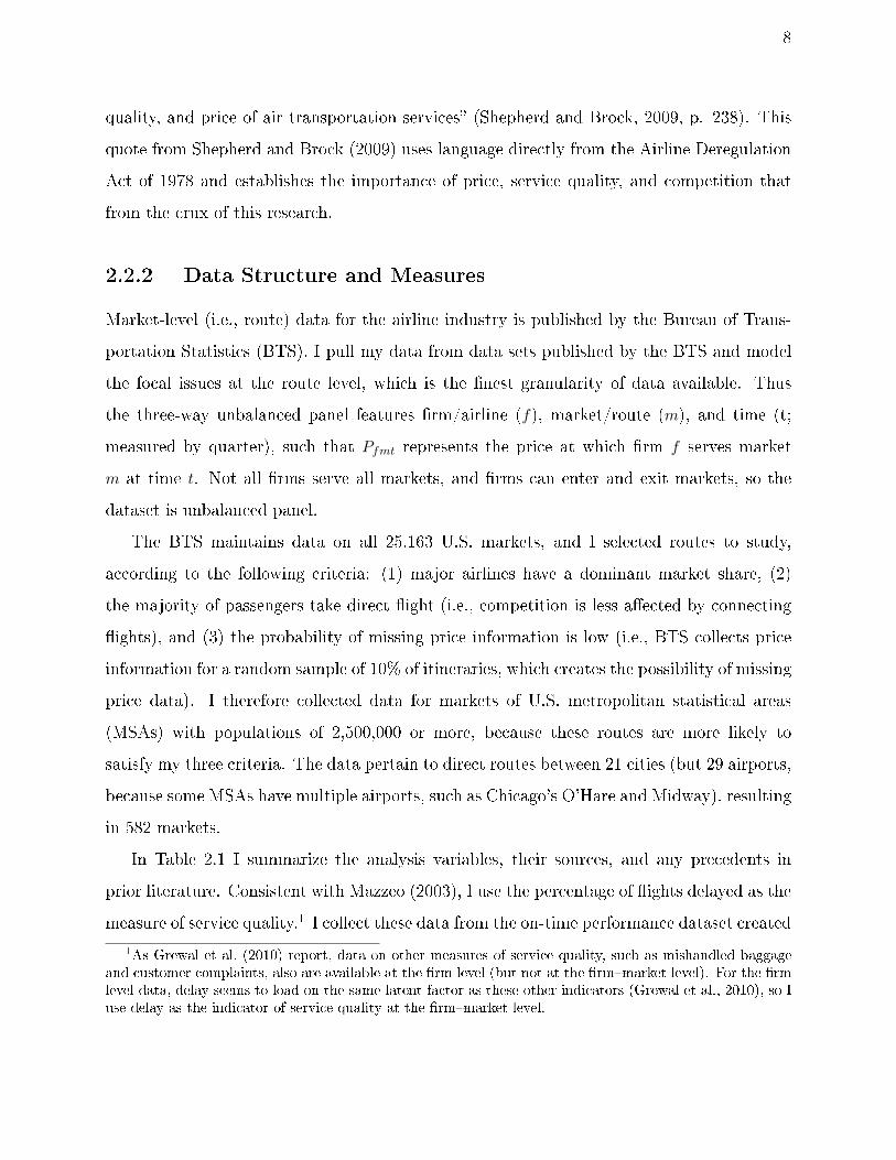
2.2.2 Data Structure and Measures
Market-level (i.e., route) data for the airline industry is published by the Bureau of Trans-
portation Statistics (BTS). I pull my data from data sets published by the BTS and model
the focal issues at the route level, which is the nest granularity of data available. Thus
the three-way unbalanced panel features rm/airline (f), market/route (m), and time (t;
measured by quarter), such that Pfmt represents the price at which rm f serves market
m at time t. Not all rms serve all markets, and rms can enter and exit markets, so the
dataset is unbalanced panel.
The BTS maintains data on all 25,163 U.S. markets, and I selected routes to study,
according to the following criteria: (1) major airlines have a dominant market share, (2)
the majority of passengers take direct ight (i.e., competition is less aected by connecting
ights), and (3) the probability of missing price information is low (i.e., BTS collects price
information for a random sample of 10% of itineraries, which creates the possibility of missing
price data). I therefore collected data for markets of U.S. metropolitan statistical areas
(MSAs) with populations of 2,500,000 or more, because these routes are more likely to
satisfy my three criteria. The data pertain to direct routes between 21 cities (but 29 airports,
because some MSAs have multiple airports, such as Chicago's O'Hare and Midway), resulting
in 582 markets.
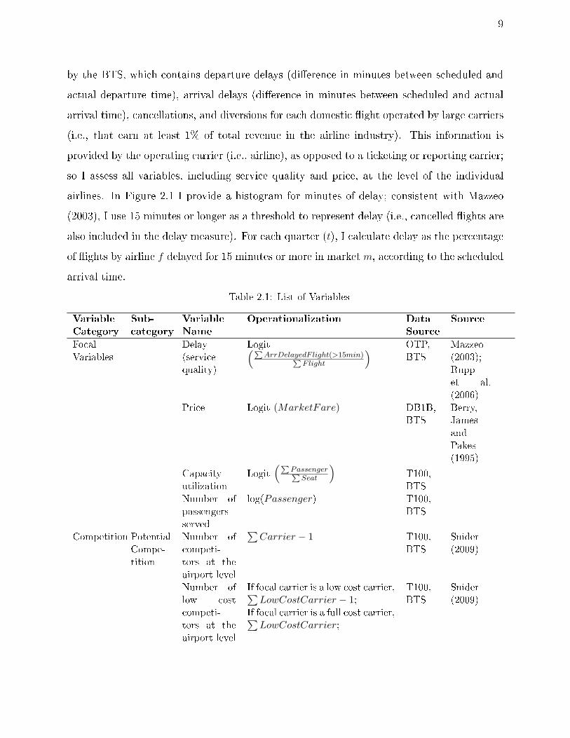
In Table 2.1 I summarize the analysis variables, their sources, and any precedents in
prior literature. Consistent with Mazzeo (2003), I use the percentage of ights delayed as the
measure of service quality.1 I collect these data from the on-time performance dataset created
1As Grewal et al. (2010) report, data on other measures of service quality, such as mishandled baggageand customer complaints, also are available at the rm level (but not at the rmmarket level). For the rmlevel data, delay seems to load on the same latent factor as these other indicators (Grewal et al., 2010), so Iuse delay as the indicator of service quality at the rmmarket level.
9
by the BTS, which contains departure delays (dierence in minutes between scheduled and
actual departure time), arrival delays (dierence in minutes between scheduled and actual
arrival time), cancellations, and diversions for each domestic ight operated by large carriers
(i.e., that earn at least 1% of total revenue in the airline industry). This information is
provided by the operating carrier (i.e., airline), as opposed to a ticketing or reporting carrier;
so I assess all variables, including service quality and price, at the level of the individual
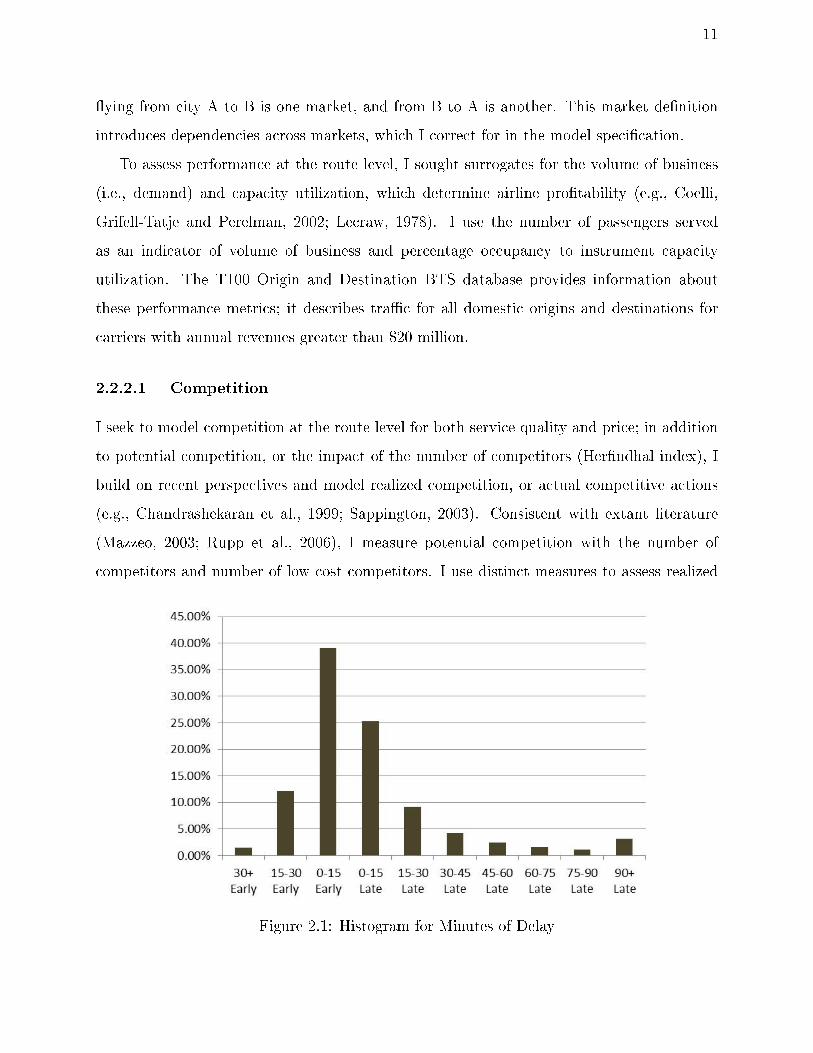
airlines. In Figure 2.1 I provide a histogram for minutes of delay; consistent with Mazzeo
(2003), I use 15 minutes or longer as a threshold to represent delay (i.e., cancelled ights are
also included in the delay measure). For each quarter (t), I calculate delay as the percentage
of ights by airline f delayed for 15 minutes or more in market m, according to the scheduled
arrival time.
Table 2.1: List of Variables
Variable
Category
Sub-
category
Variable
Name
Operationalization Data
Source
Source
FocalVariables
Delay(servicequality)
Logit(∑ArrDelayedF light(>15min)∑
Flight
) OTP,BTS
Mazzeo(2003);Ruppet al.(2006)
Price Logit (MarketFare) DB1B,BTS
Berry,JamesandPakes(1995)
Capacityutilization
Logit(∑
Passenger∑Seat
)T100,BTS
Number ofpassengersserved
log(Passenger) T100,BTS
Competition PotentialCompe-tition
Number ofcompeti-tors at theairport level
∑Carrier − 1 T100,
BTSSnider(2009)
Number oflow costcompeti-tors at theairport level
If focal carrier is a low cost carrier,∑LowCostCarrier − 1;
If focal carrier is a full cost carrier,∑LowCostCarrier;
T100,BTS
Snider(2009)

10
Number ofcompetitorsat the citylevel (notused in theestimation)
If the focal carrier operates in an-other airport in the same MSA,∑
CarrierMSAlevel − 2;If the focal carrier does not oper-ate in another airport in the sameMSA,
∑CarrierMSAlevel − 1
T100,BTS
Number oflow costcompetitorsat the citylevel (notused in theestimation)
If the focal carrieris a low cost carrier,∑
LowCostCarrierMSAlevel − 1;If the focal carrier isnot a low cost carrier,∑
LowCostCarrierMSAlevel
T100,BTS
RealizedCompe-tition
Competitormean price
Given a route,∑carrier
price−pricefocalCarrier∑Carrier−1
DB1B,BTS
Pauwels(2004)
Competitormean delay
∑carrier
dealy−delayfocalCarrier∑Carrier−1 OTP,
BTSPauwels(2004)
ControlVariables
MarketPower
Networksize
Total number of ights departingfrom the same origin for the focalcarrier
T100,BTS
Multi-airportoperations
Total number of airports the fo-cal carrier operates in the originMSA-1
T100,BTS
CongestionControl
Congestionof originairport
Total ights departure from thefocal origin airport
T100,BTS
Mazzeo(2003);Ruppet al.(2006)
Notes: I do not use congestion of destination because of its high correlation with congestion oforigin (0.999).OTP stands for On-Time Performance.
I collect data on price from the origin and destination DB1B dataset produced by the
BTS. Every quarter, this data set provides a 10% sampling of all domestic origin and des-
tination itineraries, listing airline information (ticketing carrier, operating carrier, reporting
carrier), number of connections, and itinerary price. I retain only the nonstop itineraries, to
match price information with service quality information at the ight level. To avoid coding
errors and bias due to frequent ier benets, I follow Snider (2009) and retain only observa-
tions whose itinerary prices range from $50 to $5000. For each quarter, I take the average
price of itineraries for each rmmarketquarter level, where the market is each origin
destination route combination. That is, each city pair provides two markets (Mazzeo, 2003):
11
ying from city A to B is one market, and from B to A is another. This market denition
introduces dependencies across markets, which I correct for in the model specication.
To assess performance at the route level, I sought surrogates for the volume of business
(i.e., demand) and capacity utilization, which determine airline protability (e.g., Coelli,
Grifell-Tatje and Perelman, 2002; Lecraw, 1978). I use the number of passengers served
as an indicator of volume of business and percentage occupancy to instrument capacity
utilization. The T100 Origin and Destination BTS database provides information about
these performance metrics; it describes trac for all domestic origins and destinations for
carriers with annual revenues greater than $20 million.
2.2.2.1 Competition
I seek to model competition at the route level for both service quality and price; in addition
to potential competition, or the impact of the number of competitors (Herndhal index), I
build on recent perspectives and model realized competition, or actual competitive actions
(e.g., Chandrashekaran et al., 1999; Sappington, 2003). Consistent with extant literature
(Mazzeo, 2003; Rupp et al., 2006), I measure potential competition with the number of
competitors and number of low cost competitors. I use distinct measures to assess realized
Figure 2.1: Histogram for Minutes of Delay

12
competition for service quality and price; for the former, I use the average percentage of delay
by competitors in the same route and, for the latter, I use the average price of competitors
on the same route.2
2.2.2.2 Control Variables
Consistent with extant literature (Mazzeo, 2003; Rupp et al., 2006), I control for airport
congestion factors when estimating the competition eects on ight delay. Because the
correlation between origin airport congestion and destination airport congestion is fairly high
(ρ > .80), I do not include a variable for destination airport congestion. In addition, market
power, conceptualized as the size of a carrier's operations at the endpoints of the route
(Borenstein, 1989; Evans and Kessides, 1993), inuences organizational strategic pricing
decisions (Borenstein, 1989; Kim and Singal, 1993) and also should inuence service quality
decisions. On one hand, as a rm's market power increases, service quality should decrease,
because the rm can sell without emphasizing its service quality; on the other hand, for
airlines, as market power increases, the rm takes a disproportionate amount of airport
resources and thus might oer greater service quality. I use two variables to assess market
power: network size (Borenstein, 1989; Morrison and Winston, 1996), equal to the number of
ights departing from the origin airport, and multi-airport occupation (Levine, 2009), which
is the number of origin airports that the focal airline serves in a MSA.3
2Because some large MSAs have more than one airport, carriers might face competition from other carriersthat operate in the same city pair but dierent airports (though my route denition is airport specic, suchthat Midway to Seattle is a dierent route than O'Hare to Seattle). Each carrier also might operate in morethan one airport in a MSA. Route-level competition variables correlate highly with city-level competitionvariables, and conceptually, I am interested in route (market)-level competition, so I only include market-levelvariables in the model.
3Similar to extant research (e.g., Berry, Carnall and Spiller, 2006; Berry and Jia, 2010), I might haveused a dummy variable to indicate if the origin airport is a hub for an airline; however, as I elaborate later,I needed to take a rst dierence to estimate the model, which would wipe out any dummy variable for thehub (i.e., I control for the hub airport). The network size of an airline typically increases if an airport is itshub; thus, network size provides a continuous measure of market power at the market/route level.

13
2.2.2.3 Missing Data
The DB1B dataset, from which I get information on prices, oers a 10% sampling of all
domestic itineraries, and in these selected markets/routes, I nd 11.41% (5,746 observations)
with missing values; the missing price are not negligible (Little and Rubin, 1987). I contacted
the person who manages the DB1B dataset to determine potential reasons for the missing
price values, other than the random sampling error. First, some itineraries represent frequent
iers using their rewards to y, in which case the price is recorded as $0 or nearly so. If I
remove outliers (price data outside the $50$5000 range; Snider 2009), I attain more complete
price data.4 Second, bulk fares that airlines provide to travel agents provide airlines with
no information about the price. As I detail in the next section, I use multiple imputation
methods to estimate the missing values (Little and Rubin, 1987). Finally, in .09% (43) of the
observations, information on delay, the measure of service quality, is missing. Because this
missing information mainly comes from small airlines, I dropped these observations, because
it is unlikely that excluding these cases would bias the estimation.5
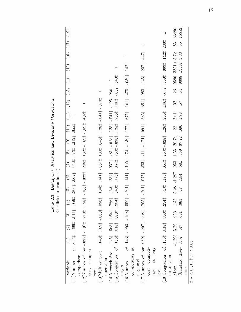
2.2.3 Descriptive Analysis
To gain further insights into the data, I carried out in-depth, univariate, descriptive analyses
of the endogenous variables: service quality, price, number of passengers served, and capacity
utilization (for descriptive statistics see Table 2.2 and Table 2.3). Service quality and capacity
utilization both are measured on a [0, 1] scale, so I logit transformed them to rescale the
variables to a (−∞,+∞) scale (Barnhart and Rosenstein, 1998; Cook and Weisberg, 1994).
Price is always positive, so I also follow extant literature and log-transformed prices (Baltagi
and Levin, 1986; Berry et al., 1995). Finally, to reduce the inuence of outliers, I log-
transformed the number of passengers served (Baltagi and Levin, 1986).
4As more and more people join frequent ier programs, the chance of sampling customers using rewardmiles should increase over time. This intuition is conrmed; the percentage of missing data shows anincreasing trend. The most missing price data occurred in 2003 (44% missing). There was not muchvariation in missing data across quarters, with a low of 10.56% in the third quarter and a high of 12.46% inthe second quarter. In terms of airlines, the highest percentage of missing data referred to American Airlines(24.39%), and the lowest was for Southwest Airlines (3.23%).
5As I report in Section 2.5.1., I assessed the accuracy of my imputation method using data from 1993 to2002 for which there are no missing values; I obtained reasonable accuracy in imputing missing values.

14
Table
2.2:
Descriptive
StatisticsandBivariate
Correlation
Coe
cients
Variable
(1)
(2)
(3)
(4)
(5)
(6)
(7)
(8)
(9)
(10)
(11)
(12)
(13)
(14)
(15)
(16)
(17)
(18)
(1)Logit(delay)
1(2)Log(price)
.089‡
1(3)Logit(capacity
utilization)
.036‡.087‡
1
(4)Log(number
ofpassengers
served)
.121‡-.026‡
.333‡
1
(5)Log(Price)
(t-
1).082‡.869‡.090‡-.031‡
1
(6)Logit(delay(t-
1))
.628‡.083‡.042‡.124‡
.089‡
1
(7)Logit(capacity
utilization
(t-1))
.030‡.097‡.812‡.276‡
.080‡.038‡
1
(8)Log(number
ofpassengers
served
(t-1))
.125‡-.029‡
.266‡.960‡-.036‡
.117‡.319‡
1
(9)Com
petitor
meanprice
.052‡.559‡
.001
-.115‡
.540‡.041‡.001
-.119‡
1
(10)Com
petitor
meandelay
.428‡.063‡.011†.027‡
.055‡.287‡.012†.034‡.059‡
1
‡p<0.01.†p<0.05.
15
Table
2.3:
Descriptive
StatisticsandBivariate
Correlation
Coe
cients(continued)
Variable
(1)
(2)
(3)
(4)
(5)
(6)
(7)
(8)
(9)
(10)
(11)
(12)
(13)
(14)
(15)
(16)
(17)
(18)
(11)Number
ofcompetitors
.063‡-.306‡
-.044‡
-.059‡
-.300‡
.062‡-.046‡
.073‡-.212‡
.055‡
1
(12)Number
oflow
cost
competi-
tors
-.027‡
-.197‡
.210‡
.128‡-.188‡
-.022†
.208‡.132‡-.189‡
-.027‡
.402‡
1
(13)Multi-airport
operation
.140‡
.102‡-.060‡
.096‡
.104‡
.141‡-.061‡
.100‡.045‡
.128‡-.041‡
-.078‡
1
(14)Networksize
.225‡
.063‡
.064‡
.286‡
.062‡
.232‡
.057‡.281‡-.028‡
.128‡-.041‡
-.005.066‡
1(15)Congestion
oforigin
.168‡
.038‡
.070†
.254‡
.040‡
.176‡
.055‡.250‡-.028‡
.125‡
.236‡
.100‡-.007.540‡
1
(16)Number
ofcompetitorsat
city
level
.143‡-.295‡
-.108‡
.059‡-.291‡
.141‡-.109‡
.074‡-.159‡
.177‡
.671‡
.161‡.275‡-.059‡
.142‡
1
(17)Number
oflow
cost
competi-
tors
atcity
level
.069‡-.207‡
.208‡
.205‡-.201‡
.075‡
.203‡.211‡-.171‡
.091‡
.385‡
.691‡.080‡.025‡.237‡.447‡
1
(19)Congestion
ofdestination
.168‡
.038‡
.069‡
.254‡
.040‡
.176‡
.055‡.250‡-.028‡
.126‡
.236‡
.100‡-.007.589‡.999‡.142‡.238‡
1
Mean
-1.293
5.28
.953
1.52
5.28
-1.287
.953
1.55
20.74
.22
2.01
.32
.26
9596
335103.72
.65
33490
Standarddevi-
ation
.607
.47
.691
.863
.47
.594
.681
.839
97.72
.096
1.78
.57
.54
9888
155973.33
.85
15552
‡p<0.01.†p<0.05.

16
Figure 2.2: Time Variation in Service Quality and Price for Select Routes

17
To provide insights into service quality and price at the route level, I present longitudinal
plots in Figure 2.2; each line represents an airline serving a particular route. The data in
Figure 2.2 related to service quality suggest that (1) the level of service quality provided by
each airline varies over time; (2) in each given market, there is considerable variability in
service quality across airlines; (3) the average level of service quality varies across markets;
and (4) if we were to rank airlines on service quality, that ranking also varies across markets
and over time. Similar conclusions emerge for price from the plots in Figure 2.2, except that
the price uctuations are much higher than the service quality uctuations (perhaps because
price is much easier to change).
Scrutiny of data on number of passengers shows seasonal variation; however, there also
is stickiness such that airlines that serve more passengers continue to do so over time. For
capacity utilization I nd considerable variation in the capacity utilization rankings of air-
lines; for some markets, the level of capacity utilization varies over time, whereas in others,
it remains fairly stable (plots for number of passengers served and capacity utilization are
available in supplementary document). Such variations support my eorts to develop a
market-level model.
2.3. Model Specication
I seek to develop a model that captures the interplay of service quality, price, and two
performance metrics (number of passengers served and capacity utilization) at the market
level. With the longitudinal micro-data about airlines serving various markets, I also seek to
assess the impacts of competition on service quality and on price. I highlight six key features
of the data structure and the ensuing model specication: (1) in the three-way structure,
all variables vary across rms (airlines) and markets (routes) and over time; (2) there are
four endogenous variablesservice quality (delay), price, number of passengers served, and
capacity utilization, (3) the large number of markets (582 routes) and rms (seven airlines)6
6The seven airlines are American, Continental, Delta, Northwestern, United, US Airways, and SouthwestAirlines. They are the top airlines by revenue in the United States, and their performances have been trackedconstantly by the BTS.
18
means that the cross-sectional data dimensions exceed the time dimensions (72 quarters); (4)
I have exogenous competition and control variables; (5) there is dependence among markets,
mainly due to reciprocal routes; and (6) price information is missing (11.41% observations).
My model incorporates all these data features. First, two-way data structures are com-
mon in marketing and economics (e.g., rms over time), whereas three-way data struc-
tures appear more often in gravity models in international economics (Bergstrand, 1985; Eg-
ger, 2000), where it is important to specify the requisite heterogeneity for the intercept term;
I delve into this issue in the next section. Second, because I have four endogenous variables
for every route and airline combination, I need some type of vector autoregression (VAR)
framework. Third, the large cross-section, exceeding even the time series, requires panel
data models (Baltagi, 2005). Typical panel models have only one dependent endogenous
variable,7 whereas I have four, so I turn to research on panel data to develop a panel VAR
(PVAR) specication (e.g., Holtz-Eakin, Newey and Rosen, 1987; Love and Zicchino, 2006).
Fourth, I explicitly model cross-sectional dependence in the error structure that arises from
reciprocal routes (e.g., Ahn and Schmidt, 1995; Huang, 2008; Mutl, 2009). Fifth, I discuss
the missing data mechanism and take appropriate measures to account for missing values
(Little and Rubin, 1987).
2.3.1 Three-Way Data
Most prominent panel data in marketing and economics are two-way, such as data on
rms over time, and the methods to model such data structures are well documented (e.g.,
Baltagi, 2005). Three-way panel data structure instead tends to appear in gravity models
in international economics, to model interactions among exporting and importing countries
over time (Bergstrand, 1985; Egger, 2000). Related literature suggests that it is critical to
model heterogeneity in the three sources and any potential interactions (Baltagi, Egger and
Pfaermayr, 2003). The data structure involves a three-way panel, for which each observa-
7Although there are methods to correct for the endogeneity of explanatory variables (e.g., Ahn andSchmidt, 1995; Arellano and Bond, 1991; Hsiao, Pesaran and Tahmiscioglu, 2002), my goal is to study theinterplay among service quality, price, and performance metrics, requiring contemporaneous and eects;thus, a panel VAR approach is more appropriate than just correcting for endogeneity.
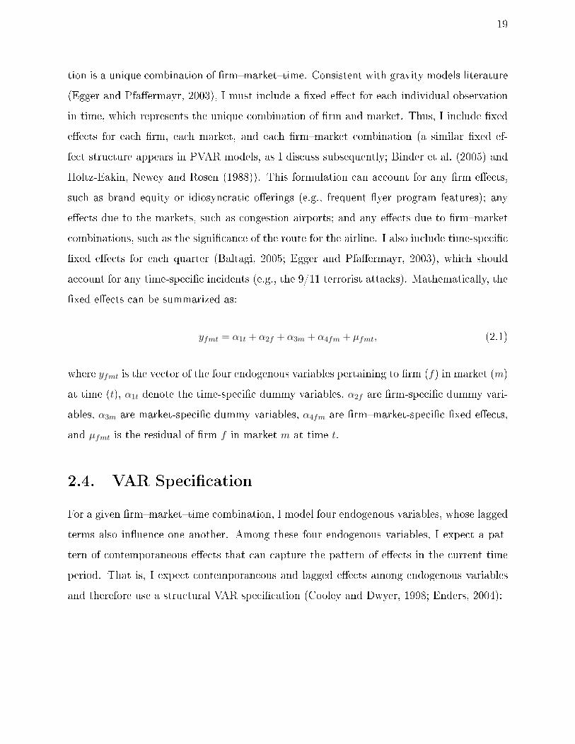
19
tion is a unique combination of rmmarkettime. Consistent with gravity models literature
(Egger and Pfaermayr, 2003), I must include a xed eect for each individual observation
in time, which represents the unique combination of rm and market. Thus, I include xed
eects for each rm, each market, and each rmmarket combination (a similar xed ef-
fect structure appears in PVAR models, as I discuss subsequently; Binder et al. (2005) and
Holtz-Eakin, Newey and Rosen (1988)). This formulation can account for any rm eects,
such as brand equity or idiosyncratic oerings (e.g., frequent yer program features); any
eects due to the markets, such as congestion airports; and any eects due to rmmarket
combinations, such as the signicance of the route for the airline. I also include time-specic
xed eects for each quarter (Baltagi, 2005; Egger and Pfaermayr, 2003), which should
account for any time-specic incidents (e.g., the 9/11 terrorist attacks). Mathematically, the
xed eects can be summarized as:
yfmt = α1t + α2f + α3m + α4fm + µfmt, (2.1)
where yfmt is the vector of the four endogenous variables pertaining to rm (f) in market (m)
at time (t), α1t denote the time-specic dummy variables, α2f are rm-specic dummy vari-
ables, α3m are market-specic dummy variables, α4fm are rmmarket-specic xed eects,
and µfmt is the residual of rm f in market m at time t.
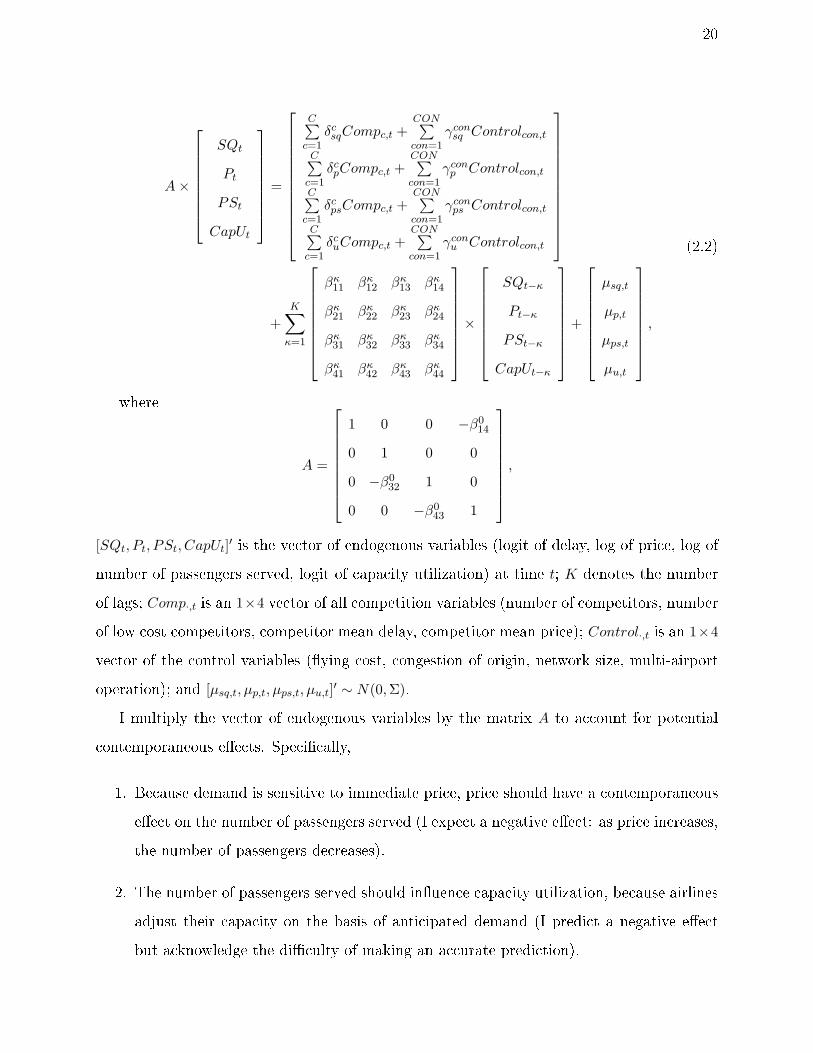
2.4. VAR Specication
For a given rmmarkettime combination, I model four endogenous variables, whose lagged
terms also inuence one another. Among these four endogenous variables, I expect a pat-
tern of contemporaneous eects that can capture the pattern of eects in the current time
period. That is, I expect contemporaneous and lagged eects among endogenous variables
and therefore use a structural VAR specication (Cooley and Dwyer, 1998; Enders, 2004):
20
A×
SQt
Pt
PSt
CapUt
=
C∑c=1
δcsqCompc,t +CON∑con=1
γconsq Controlcon,t
C∑c=1
δcpCompc,t +CON∑con=1
γconp Controlcon,t
C∑c=1
δcpsCompc,t +CON∑con=1
γconps Controlcon,t
C∑c=1
δcuCompc,t +CON∑con=1
γconu Controlcon,t
+
K∑κ=1
βκ11 βκ
12 βκ13 βκ
14
βκ21 βκ
22 βκ23 βκ
24
βκ31 βκ
32 βκ33 βκ
34
βκ41 βκ
42 βκ43 βκ
44
×
SQt−κ
Pt−κ
PSt−κ
CapUt−κ
+
µsq,t
µp,t
µps,t
µu,t
,
(2.2)
where
A =
1 0 0 −β014
0 1 0 0
0 −β032 1 0
0 0 −β043 1
,
[SQt, Pt, PSt, CapUt]′ is the vector of endogenous variables (logit of delay, log of price, log of
number of passengers served, logit of capacity utilization) at time t; K denotes the number
of lags; Comp·,t is an 1×4 vector of all competition variables (number of competitors, number
of low cost competitors, competitor mean delay, competitor mean price); Control·,t is an 1×4
vector of the control variables (ying cost, congestion of origin, network size, multi-airport
operation); and [µsq,t, µp,t, µps,t, µu,t]′ ∼ N(0,Σ).
I multiply the vector of endogenous variables by the matrix A to account for potential
contemporaneous eects. Specically,
1. Because demand is sensitive to immediate price, price should have a contemporaneous
eect on the number of passengers served (I expect a negative eect: as price increases,
the number of passengers decreases).
2. The number of passengers served should inuence capacity utilization, because airlines
adjust their capacity on the basis of anticipated demand (I predict a negative eect
but acknowledge the diculty of making an accurate prediction).
21
3. Service quality might depend on capacity utilization, because the boarding time and
ight attendants per customer vary with the number of passengers on a ight (I expect
a negative eect: as capacity utilization increases, service quality decreases).
2.4.1 Panel VAR Model
In most marketing applications of VAR, the estimated models (e.g., Pauwels, Hanssens and
Siddarth, 2002; Srinivasan, Leszczyc and Bass, 2000) exhibit long time series and small
cross-sectional units (large T, small N). Yet the data comprise 582 markets, seven airlines
(or 1,263 cross-sectional elements), but at most 72 quarters of time for each airlinemarket
combination. In other words, I have large cross-section units and short time series (small T,
large N), which makes it dicult, and perhaps meaningless, to perform several thousands
of conventional VAR estimations. To make full use of the data, I instead estimate a PVAR
model (Holtz-Eakin et al., 1988; Love and Zicchino, 2006) and estimate the coecients by
pooling all data, even as I control for individual eects at dierent levels. Thus, I combine
Equations 2.1 and 2.2 and write the PVAR model as follows (this specication poses unique
estimation challenges that I discuss in the next section; in Equation 2.3, the subscripts sq, p,
ps, and u refer to service quality, price, number of passengers served, and capacity utilization,
respectively):

22
1 0 0 −β014
0 1 0 0
0 −β032 1 0
0 0 −β043 1
×
SQt
Pt
PSt
CapUt
=
α1sqt + α2sqf + α3sqm + α4sqfm
α1pt + α2pf + α3pm + α4pfm
α1pst + α2psf + α3psm + α4psfm
α1ut + α2uf + α3um + α4ufm
+
C∑c=1
δcsqCompc,t +CON∑con=1
γconsq Controlcon,t
C∑c=1
δcpCompc,t +CON∑con=1
γconp Controlcon,t
C∑c=1
δcpsCompc,t +CON∑con=1
γconps Controlcon,t
C∑c=1
δcuCompc,t +CON∑con=1
γconu Controlcon,t
+
K∑κ=1
βκ11 βκ
12 βκ13 βκ
14
βκ21 βκ
22 βκ23 βκ
24
βκ31 βκ
32 βκ33 βκ
34
βκ41 βκ
42 βκ43 βκ
44
×
SQt−κ
Pt−κ
PSt−κ
CapUt−κ
+
µsq,t
µp,t
µps,t
µu,t
.
(2.3)
2.4.2 Cross-Sectional Dependence
I treat each unique combination of origindestination airports as a market. Because con-
sumers usually buy round-trip tickets when they travel, they likely consider price and service
quality for both the route and its reciprocal route. Thus, airlines must jointly determine
their price and service quality levels, as well as how much ight capacity to provide for
the two routes (city A to city B and its reciprocal, city B to city A). For each airlinetime
combination, the price, service quality, capacity utilization, and number of passenger served
are not independent of these same variables in connection to the reciprocal route. Instead,
price, service quality, capacity utilization, and the number of passenger served are functions
of the reciprocal route versions of those variables. I model this cross-sectional dependency

23
in a panel setting with the following equation (Huang, 2008; Mutl, 2009):
1 0 0 −β014
0 1 0 0
0 −β032 1 0
0 0 −β043 1
×
SQfabt
Pfabt
PSfabt
CapUfabt
=
α1sqt + α2sqf + α3sqab + α4sqfab
α1pt + α2pf + α3pab + α4pfab
α1pst + α2psf + α3psab + α4psfab
α1ut + α2uf + α3uab + α4ufab
+
ηsq 0 0 0
0 ηp 0 0
0 0 ηps 0
0 0 0 ηu
×
SQfbat
Pfbat
PSfbat
CapUfbat
+
K∑κ=1
βκ11 βκ
12 βκ13 βκ
14
βκ21 βκ
22 βκ23 βκ
24
βκ31 βκ
32 βκ33 βκ
34
βκ41 βκ
42 βκ43 βκ
44
×
SQfabt−κ
Pfabt−κ
PSfabt−κ
CapUfabt−κ
+
C∑c=1
δcsqCompc,fabt +CON∑con=1
γconsq Controlcon,fabt
C∑c=1
δcpCompc,fabt +CON∑con=1
γconp Controlcon,fabt
C∑c=1
δcpsCompc,fabt +CON∑con=1
γconps Controlcon,fabt
C∑c=1
δcuCompc,fabt +CON∑con=1
γconu Controlcon,fabt
+
µsq,fabt
µp,fabt
µps,fabt
µu,fabt
(2.4)
where η· are the coecients of the endogenous variables in the paired market. For ease
of presentation, I distinguish the market subscript into ab, such that a indicates the origin
airport, and b stands for the destination airport.
2.4.3 Missing Data
I sought the best possible approach to manage the missing price data. Consistent with
extant literature (Little and Rubin, 1987; Schafer, 1997), I rst attempted to understand
whether the mechanism entailed missing completely at random (MCAR), missing at random
(MAR), or not missing at random (NMAR) (Rubin, 1976). I follow conventions and denote
Y = (yij) as the data matrix, such that Yobs represents the observed component, and Ymis
is the missing component; in the missing data indicator matrix M = (mij), mij = 1 if yij
is missing and mij = 0 if yij is present. The missing data mechanism (MCAR, MAR, or
NMAR) is dened as the conditional distribution of M given Y , such that f(M |Y, ϕ) where ϕ
denotes unknown parameters, I determine that (1) MCAR implies that missing data do not

24
depend on the value of the data, missing or observed, such that f(M |Y, ϕ) = f(M |ϕ)∀Y, ϕ;
(2) MAR makes a less restrictive assumption, and missing data depend only on the Yobs
component, not the Ymis component, or f(M |Y, ϕ) = f(M |Yobs, ϕ)∀Ymis, ϕ; and (3) NMAR is
critical when M depends on Ymis (Little and Rubin, 1987; Schafer, 1997).
In the dataset, the missing data pertain only to prices and appear largely the result of
frequent ier programs and bulk fares. Thus, the missing data do not relate to the price of
the ticket (NMAR is irrelevant), and observed data (Yobs) are informative about the missing
data (Ymis)), because they come from the same airline, market (route), and/or time (MCAR
is too restrictive). Thus, MAR provides the most appropriate missing data mechanism.
If θ denotes the parameters for the data generation process for Y = (Yobs, Ymis), then with
an MAR assumption, I can write the joint probability of η = (θ, ϕ) as:
Pr[θ, ϕ|Yobs,M ] ∝ Pr[M,Yobs|θ, ϕ]π(θ, ϕ) ∝ Pr[M |Yobs, ϕ] Pr[Yobs|θ]π(θ, ϕ) (2.5)
where π(θ, ϕ) is the joint prior distribution. Assuming independent priors for θ and ϕ, I also
can rewrite Equation 2.5 as:
Pr[θ, ϕ|Yobs,M ] ∝ Pr[M |Yobs, ϕ] Pr[Yobs|θ]πθ(θ)πϕ(ϕ) (2.6)
Because I seek statistical inferences about θ, I derive the marginal posterior for θ by
integrating out ϕ from Equation 2.6, which provides:
Pr[θ|Yobs,M ] =
∫Pr[θ, ϕ|Yobs,M ]dϕ ∝ Pr[Yobs|θ]πθ(θ)
∫Pr[M |Yobs, ϕ]πϕ(ϕ)dϕ (2.7)
The integral on the right-hand side of the equation does not depend on θ, so I rewrite
Equation 2.7 as follows:
Pr[θ|Yobs,M ] = L[θ|Yobs]πϕ(ϕ). (2.8)
Finally, because the inference of θ does not depend on ϕ, I resort to data imputation for
the missing values and draw inferences of θ (Little and Rubin, 1987; Schafer, 1997); I provide
the details of this imputation in the next section.
25
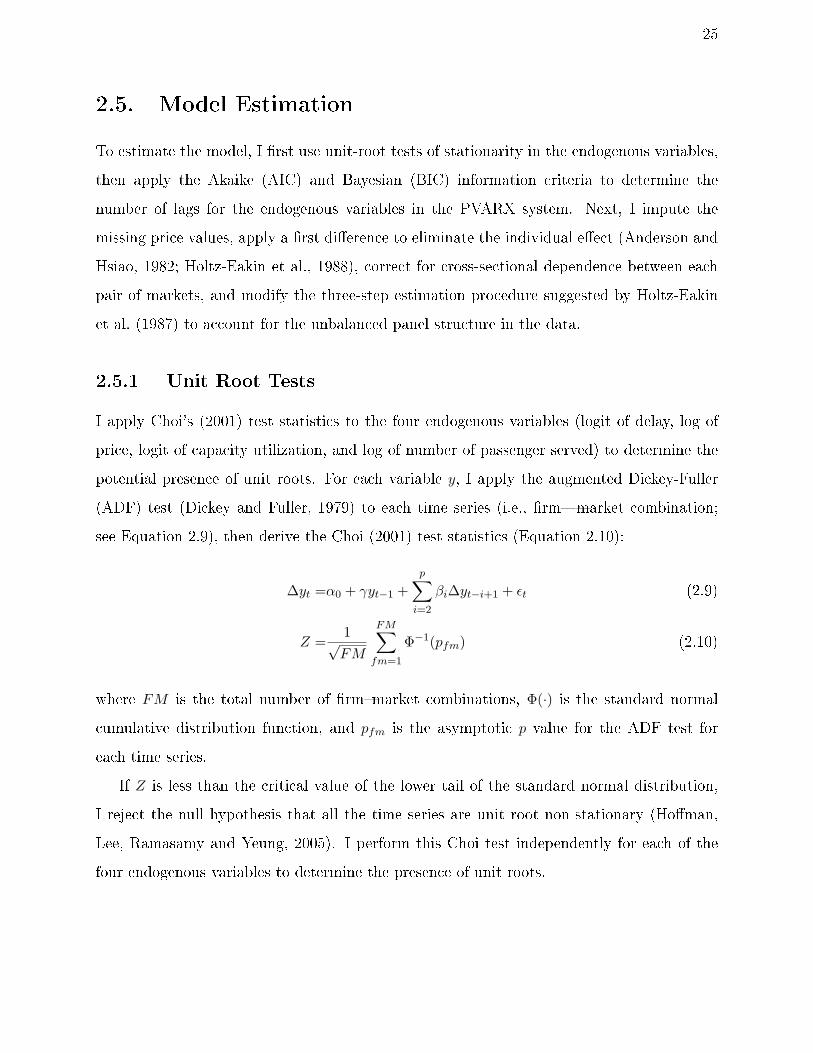
2.5. Model Estimation
To estimate the model, I rst use unit-root tests of stationarity in the endogenous variables,
then apply the Akaike (AIC) and Bayesian (BIC) information criteria to determine the
number of lags for the endogenous variables in the PVARX system. Next, I impute the
missing price values, apply a rst dierence to eliminate the individual eect (Anderson and
Hsiao, 1982; Holtz-Eakin et al., 1988), correct for cross-sectional dependence between each
pair of markets, and modify the three-step estimation procedure suggested by Holtz-Eakin
et al. (1987) to account for the unbalanced panel structure in the data.
2.5.1 Unit Root Tests
I apply Choi's (2001) test statistics to the four endogenous variables (logit of delay, log of
price, logit of capacity utilization, and log of number of passenger served) to determine the
potential presence of unit roots. For each variable y, I apply the augmented Dickey-Fuller
(ADF) test (Dickey and Fuller, 1979) to each time series (i.e., rmmarket combination;
see Equation 2.9), then derive the Choi (2001) test statistics (Equation 2.10):
∆yt =α0 + γyt−1 +
p∑i=2
βi∆yt−i+1 + ϵt (2.9)
Z =1√FM
FM∑fm=1
Φ−1(pfm) (2.10)
where FM is the total number of rmmarket combinations, Φ(·) is the standard normal
cumulative distribution function, and pfm is the asymptotic p value for the ADF test for
each time series.
If Z is less than the critical value of the lower tail of the standard normal distribution,
I reject the null hypothesis that all the time series are unit root non-stationary (Homan,
Lee, Ramasamy and Yeung, 2005). I perform this Choi test independently for each of the
four endogenous variables to determine the presence of unit roots.
26
2.5.2 Number of Lags
To determine the appropriate number of lags, I run univariate models for each endogenous
variable, with lags of the endogenous variable, the xed eects, and the control variables.
Then I determine the number of lags that produces the lowest AIC and BIC values. The
exact model specication is:
yfmt =α1 + α2f + α3y + α4q +
k∑i=1
βkyfm(t−k)
+ γ1HubOfmt + γ2HubDfmt + γ3Distancem + γ4PopGeoMeanmt,
(2.11)
where α1 is the intercept, α2f is the rm-xed eect, α3y is the year-xed eect; α4q is
the quarter-xed eect; HubOfmt is an indicator of whether the focal airline has a hub in
the origin airport; HubDfmt is an indicator of whether the focal airline has a hub in the
destination airport; Distancem is the distance between the origin airport and the destination
airport; and PopGeoMeanmt is the geometric mean of the populations in the origin city and
the destination city at time t.
2.5.3 Missing Data
To impute missing price values, I create a matrix with information on price (observed and
missing) and information on all other variables. First, I include price information that
comprises three variables, namely, the rst lag of price (if unavailable, I use the most recent
lag value), the average price of the focal carrier across all markets, and the rst lag of price for
the focal carrier across all markets. Second, the matrix features four competition variables:
the change in the average price of competitors in the current period; the average price per
mile (i.e., average yield) for the route, calculated as the average price over all airlines that
had price values available ying that route, which I divided by the distance in miles for that
route; the number of competitors on the route; and number of low cost competitors on the
route. Third, as airline variables, I used the number of passengers served, number of ights
from the origin, market share, average delay in minutes, percentage of cancellations, number
of airports the focal airline serves in the same MSA, percentage of departures performed in

27
the market, and age of the focal airline. Fourth, I included two market-specic two variables,
distance in miles and the geometric mean of the populations in the origin and destination
cities. Fifth, the time variables were gross domestic product and jet fuel market price.
I estimate the missing values using an iterative, two-step procedure (Darmawan, 2002;
Little and Rubin, 1987; Schafer, 1997). In step 1, I impute the missing values by random
draws from a conditional multivariate normal distribution (60 simulated iterations with an
uninformative prior; Schafer (1997)), given the observed data and current covariance matrix
of all the variables. In step 2, I update the covariance matrix with by a Bayesian posterior
distribution, given the observed data and most recent imputed missing values. I repeatedly
iterate between these two steps until I achieve convergence.
2.5.4 Unobserved Heterogeneity
I use rm-, market-, and time-specic xed eects, as well as xed eects for each rm
market to account for unobserved heterogeneity (see Equations 2.1, 2.2, and 2.4). I cannot
estimate these xed eects, because they correlate with the error term, due to presence of
lagged endogenous variables (e.g., Holtz-Eakin et al., 1987; Holtz-Eakin et al., 1988; Lund-
berg, 1985). Instead, I apply a rst dierence to Equation 2.4 to eliminate individual eects
(Anderson and Hsiao, 1982; Arellano and Bond, 1991; Holtz-Eakin et al., 1988) and thus can

28
rewrite the equation as:
1 0 0 −β014
0 1 0 0
0 −β032 1 0
0 0 −β043 1
×
∆SQfabt
∆Pfabt
∆PSfabt
∆CapUfabt
=
ηsq 0 0 0
0 ηp 0 0
0 0 ηps 0
0 0 0 ηu
×
∆SQfbat
∆Pfbat
∆PSfbat
∆CapUfbat
+
β0sqt +C∑c=1
δcsq∆Compc,fabt +CON∑con=1
γconsq ∆Controlcon,fabt
β0pt +C∑c=1
δcp∆Compc,fabt +CON∑con=1
γconp ∆Controlcon,fabt
β0pst +C∑c=1
δcps∆Compc,fabt +CON∑con=1
γconps ∆Controlcon,fabt
β0ut +C∑c=1
δcu∆Compc,fabt +CON∑con=1
γconu ∆Controlcon,fabt
+
K∑κ=1
βκ11 βκ
12 βκ13 βκ
14
βκ21 βκ
22 βκ23 βκ
24
βκ31 βκ
32 βκ33 βκ
34
βκ41 βκ
42 βκ43 βκ
44
×
∆SQfabt−κ
∆Pfabt−κ
∆PSfabt−κ
∆CapUfabt−κ
+
νsq,fabt
νp,fabt
νps,fabt
νu,fabt
(2.12)
The only xed eects left after rst dierencing the equations are the time-specic eects,
denoted β0·t = α1·t−α1·t−1. In Equation 2.12, the lagged dependent variables are endogenous,
because they correlate with the error terms (Anderson and Hsiao, 1982; Arellano and Bond,
1991). For each ∆yit−k, yit−k−1 serves as an instrumental variable, because it correlates
with ∆yit−k but is orthogonal to the error term (Anderson and Hsiao, 1982). To estimate
Equation 2.12, I use the general method of moments, which is based on the orthogonality
condition of instruments (i.e., yit−k−1, ∆Xit ) and νit (Anderson and Hsiao, 1982; Holtz-Eakin
et al., 1988).
2.5.5 Cross-Sectional Dependence
To account for the interdependence of each endogenous variable between each pair of markets,
I estimate the level of cross-sectional dependence, denoted ρ, then treat ρ as data when I
implement the three-step PVAR estimation, as I detail in Section 2.4.6. (Mutl, 2009).
29
2.5.5.1 Stage 1: Instrumental variable regression to each equation in the VAR
system
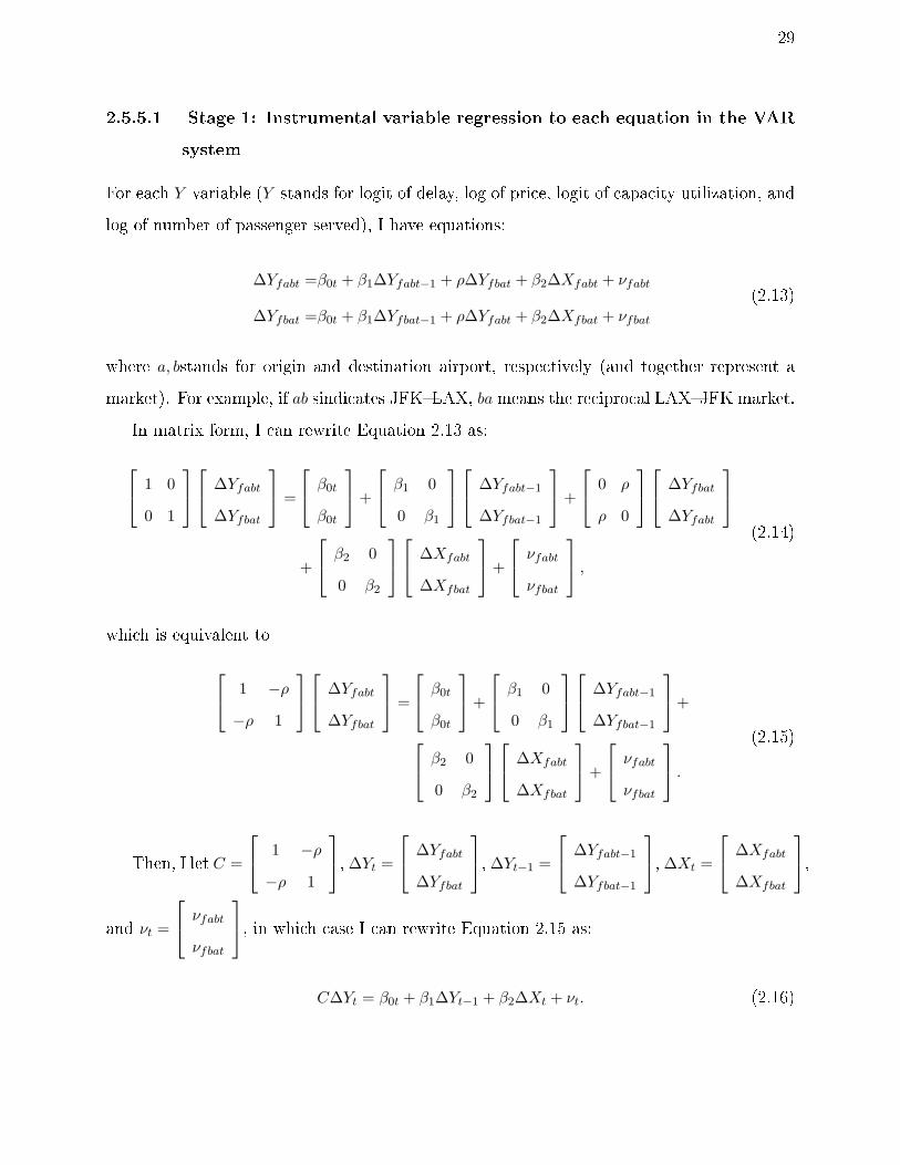
For each Y variable (Y stands for logit of delay, log of price, logit of capacity utilization, and
log of number of passenger served), I have equations:
∆Yfabt =β0t + β1∆Yfabt−1 + ρ∆Yfbat + β2∆Xfabt + νfabt
∆Yfbat =β0t + β1∆Yfbat−1 + ρ∆Yfabt + β2∆Xfbat + νfbat
(2.13)
where a, bstands for origin and destination airport, respectively (and together represent a
market). For example, if ab sindicates JFKLAX, ba means the reciprocal LAXJFK market.
In matrix form, I can rewrite Equation 2.13 as:
1 0
0 1
∆Yfabt
∆Yfbat
=
β0t
β0t
+
β1 0
0 β1
∆Yfabt−1
∆Yfbat−1
+
0 ρ
ρ 0
∆Yfbat
∆Yfabt
+
β2 0
0 β2
∆Xfabt
∆Xfbat
+
νfabt
νfbat
,
(2.14)
which is equivalent to
1 −ρ
−ρ 1
∆Yfabt
∆Yfbat
=
β0t
β0t
+
β1 0
0 β1
∆Yfabt−1
∆Yfbat−1
+
β2 0
0 β2
∆Xfabt
∆Xfbat
+
νfabt
νfbat
.
(2.15)
Then, I let C =
1 −ρ
−ρ 1
, ∆Yt =
∆Yfabt
∆Yfbat
, ∆Yt−1 =
∆Yfabt−1
∆Yfbat−1
, ∆Xt =
∆Xfabt
∆Xfbat
,and νt =
νfabt
νfbat
, in which case I can rewrite Equation 2.15 as:
C∆Yt = β0t + β1∆Yt−1 + β2∆Xt + νt. (2.16)

30
If I multiply Equation 2.16 by C−1, I obtain:
∆Yt = C−1β0t + C−1β1∆Yt−1 + C−1β2∆Xt + C−1νt. (2.17)
Finally, using Yt−2 to instrument ∆Yt−1, and applying an IV regression to Equation 2.16
, I derive the tted value C−1νt of the residual in Equation 2.17 .
2.5.5.2 Stage 2: Estimate ρ
After collecting C−1νt from stage 1, I can estimate C−1 on the basis of Cov(C−1νt), where νt
is assumed to be distributed i.i.d N(0, σ2): Cov(C−1νt) = E(C−1νtν′tC
−1′) = C−1E(νtν
′t)C
−1′=
C−1σ2C−1′. I also can estimate ρ on the basis of C−1.
2.5.5.3 Stage 3: Estimate the PVARX model with ρ
If I insert ρ into Equation 2.14, I obtain:
1 0
0 1
∆Yfabt
∆Yfbat
=
β0t
β0t
+
β1 0
0 β1
∆Yfabt−1
∆Yfbat−1
+
0 ρ
ρ 0
∆Yfbat
∆Yfabt
+
β2 0
0 β2
∆Xfabt
∆Xfbat
+
νfabt
νfbat
,
(2.18)
I treat ρ as data to compute a new set of dependent variables, and I estimate the model
using the PVARX estimation procedures described in Section 2.4.6. (Huang, 2008; Mutl,
2009):
1 0
0 1
−
0 ρ
ρ 0
∆Yfbat
∆Yfabt
=
β0t
β0t
+
β1 0
0 β1
∆Yfabt−1
∆Yfbat−1
+
β2 0
0 β2
∆Xfabt
∆Xfbat
+
νfabt
νfbat
,
(2.19)

31
2.5.6 PVAR Estimation
Now that I have rst dierenced the VARX system to remove various xed eects, corrected
for cross-sectional dependence, and multiplied both sides of the VARX system by C−1 (the
inverse of the matrix capturing contemporaneous eects among endogenous variables), I
can apply the three-stem procedure proposed by Holtz-Eakin et al. (1987) to estimate the
PVARX model.
First, I use two-stage least square estimates of on each endogenous variable for each time
period (i.e., estimate Equation 2.12 for each time period, and treat β0·t as the intercept),
using the following two-stage least square estimator:
Bt = [W ′tZt(Z
′tZt)
−1Z ′tWt]
−1W ′tZt(Z
′tZt)
−1Z ′tYt, (2.20)
where Wt is the regressor vector, and Zt is the instrument vector (i.e., yit−k−1,∆Xit ). Then
I can calculate a vector of residuals for period t: νt = Yt −WtBt.
Second, to construct the weighting matrix E(Z ′V V ′Z) , I use:
Ω =
N∑i=1
(νirνisZ′irZis)/N (2.21)
where νit, t = r, s is the ith element (observation) of Vt, Zit is the ith row of Zt, and N is the
number of observations in each time period.
Third, to obtain a generalized least squares estimator of the entire parameter vector, I
stack all four endogenous variables and use all available observations, as specied in Equa-
tion 2.12. Because I have 72 time periods, I dene βt = βq + λX∆Xt + λDDt, where q = 4 for
change in quarter 1 → 2, 2 → 3, 3 → 4, or 4 → 1, and Dt = 1, if q = 2 → 3, 3 → 4 in year 2001
and q = 4 → 1, 1 → 2 in year 2002. Thus,
Bt = [W ′ZΩ−1Z ′W ]−1W ′ZΩ−1Z ′Y, (2.22)
This three-step estimation procedure (Holtz-Eakin et al., 1987) applies to balanced panel
data, so I must adapt it to the unbalanced panel setting, in which the number of rms varies
32
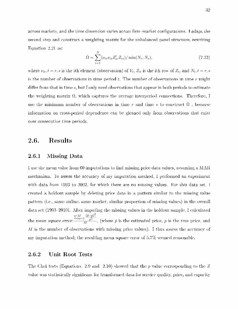
across markets, and the time dimension varies across rmmarket congurations. I adapt the
second step and construct a weighting matrix for the unbalanced panel structure, rewriting
Equation 2.21 as:
Ω =
N∑i=1
(νirνisZ′irZis)/min(Nr, Ns), (2.23)
where νit, t = r, s is the ith element (observation) of Vt, Zit is the ith row of Zt, and Nt, t = r, s
is the number of observations in time period t. The number of observations in time r might
dier from that in time s, but I only need observations that appear in both periods to estimate
the weighting matrix Ω, which captures the average interperiod connections. Therefore, I
use the minimum number of observations in time r and time s to construct Ω , because
information on cross-period dependence can be gleaned only from observations that exist
over consecutive time periods.
2.6. Results
2.6.1 Missing Data
I use the mean value from 60 imputations to nd missing price data values, assuming a MAR
mechanism. To assess the accuracy of my imputation method, I performed an experiment
with data from 1993 to 2002, for which there are no missing values. For this data set, I
created a holdout sample by deleting price data in a pattern similar to the missing value
pattern (i.e., same airline, same market, similar proportion of missing values) in the overall
data set (19932010). After imputing the missing values in the holdout sample, I calculated
the mean square error:
∑Mm=1
(p−p)2
p2
M , (where p is the estimated price, p is the true price, and
M is the number of observations with missing price values). I thus assess the accuracy of
my imputation method; the resulting mean square error of 5.7% seemed reasonable.
2.6.2 Unit Root Tests
The Choi tests (Equations 2.9 and 2.10) showed that the p value corresponding to the Z
value was statistically signicant for transformed data for service quality, price, and capacity

33
Table 2.4: Cross-Sectional Dependence
Dependent Variable Cross-Sectional Dependence
Service Quality (logit(delay)) .153** (.01)log(Price) .245* (.07)logit(CapUtilization) .260** (.05)log(Number of Passenger Served) .250** (.04)
Notes: Standard errors are in parentheses.*p < 0.01 ** p < 0.001.
utilization (p < .01); that is, the data-generating processes for these three variables appear
stationary. For number of passengers served, the p-value corresponding to Z is marginally
statistically signicant (< .06), which suggests the possibility of a unit root; however, the
rst dierence for the number of passengers served data series is stationary (p < .01). As
I elaborate in the PVAR estimation, I rst dierence the data to eliminate the individual
eects (Anderson and Hsiao, 1982; Holtz-Eakin et al., 1988), which makes the data series
for number of passengers served stationary. Thus, I am not concerned about any unit root
issues among the four endogenous variables.
2.6.3 Number of Lags
The lowest AIC and BIC values, from the estimation of Equation 10, result when I use one
lag for each of the four endogenous variables. I use this one-lag value in all the models.
2.6.4 Cross-Sectional Dependence
I nd evidence of cross-sectional dependence (Equation 18), in that the estimates of ρ are
positive for the four endogenous variables (see Table 2.4). These results conrm the idea that
most passengers buy round-trip tickets. Thus, the service quality, price, and performance
metrics are positively related for reciprocal routes.
2.6.5 Panel VAR
I present the results of my PVAR estimation in Table 2.5. I estimate the contemporaneous
eects (Equation 2.2) from the variance-covariance matrix of the residuals. The results

34
suggest that as price increases, the number of passengers served decreases (β32 = −0.873,
p < .01) consistent with a standard notion of a downward sloping demand curve. As the
number of passengers served increases, capacity utilization decreases (β43 = −0.758, p < .01);
to meet increasing demand, airlines apparently add capacity, which then reduces capacity
utilization. Finally, as capacity utilization increases, service quality decreases (β14 = 0.0847,
p < .05), which reinforces the basic idea that service quality declines with fuller ights
(Ramdas and Williams, 2008).
I present the estimated coecients for the lagged endogenous variables and the exogenous
variables in Table 2.6. The coecients of the endogenous variables cannot be interpreted
directly, because of the feedback mechanism among the endogenous variables, so I use impulse
response functions (IRFs) to glean insights (Hamilton, 1994). Specically, for my PVAR
system, I use coecient bootstrapping to compute the IRF (Love and Zicchino, 2006). To
calculate these IRFs, I consider a one standard deviation (1) decrease in price, (2) increase in
service quality (i.e., decrease in delay), (3) increase in capacity utilization, and (4) increase
in number of passengers served. In the IRF plots in Figures 2.3 and 2.4, I note the change in
one endogenous variable, in response to a one standard deviation shift in another endogenous
variable, over eight periods. The Y axes represent the value of the endogenous variable, and
the X axes indicate time (the shock occurs at t0, and the focal endogenous variable starts
to change at t1). As is common practice, the red concrete line indicates the dierence in the
value of the endogenous variable for the shift compared to the condition when there is no
shift (thus the x-axes can be seen as representing this no shift condition); the two dashed
lines represent the 95% condence interval bands of the red-concrete line.
2.6.5.1 Impact on Service Quality
Greater service quality, which means a decrease in delays (Figure 2.3, Panel A), improves
service quality in the next period, and this improvement persists for around ve periods,
in support of persistence in service quality. In contrast, Panel B of Figure 2.3 shows that
lower prices lead to lower service quality, which remains for four periods. Greater capacity
utilization seems to improve service quality for around four periods (Panel C, Figure 2.3),
but a change in the number of passengers served does not inuence service quality (Panel
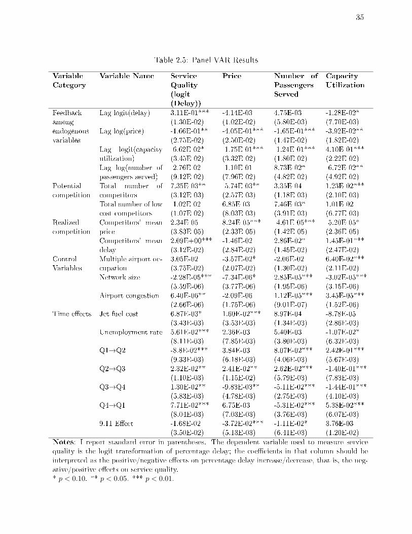
35
Table 2.5: Panel VAR Results
Variable
Category
Variable Name Service
Quality
(logit
(Delay))
Price Number of
Passengers
Served
Capacity
Utilization
Feedbackamong
Lag logit(delay) 3.11E-01***(1.30E-02)
-4.14E-03(1.02E-02)
4.75E-03(5.80E-03)
-1.28E-02*(7.70E-03)
endogenousvariables
Lag log(price) -1.66E-01**(2.75E-02)
-4.05E-01***(2.50E-02)
-1.65E-01***(1.47E-02)
-3.92E-02**(1.82E-02)
Lag logit(capacityutilization)
-6.62E-02*(3.45E-02)
-1.75E-01***(3.32E-02)
-1.24E-01***(1.80E-02)
4.10E-01***(2.22E-02)
Lag log(number ofpassengers served)
-2.76E-02(9.12E-02)
-1.10E-01(7.96E-02)
8.73E-02*(4.82E-02)
-6.72E-02**(4.92E-02)
Potentialcompetition
Total number ofcompetitors
7.35E-03**(3.12E-03)
-5.74E-03**(2.57E-03)
3.35E-04(1.18E-03)
1.23E-02***(2.10E-03)
Total number of lowcost competitors
-1.02E-02(1.07E-02)
6.85E-03(8.03E-03)
7.46E-03*(3.91E-03)
1.01E-02(6.77E-03)
Realizedcompetition
Competitors' meanprice
2.34E-05(3.83E-05)
8.24E-05***(2.33E-05)
-4.61E-05***(1.42E-05)
-5.20E-05*(2.36E-05)
Competitors' meandelay
2.09E+00***(3.12E-02)
-1.46E-02(2.84E-02)
2.86E-02*(1.45E-02)
1.45E-01***(2.47E-02)
ControlVariables
Multiple airport oc-cupation
3.05E-02(3.75E-02)
-3.57E-02*(2.07E-02)
-2.06E-02(1.30E-02)
6.40E-02***(2.11E-02)
Network size -2.28E-05***(5.59E-06)
-7.34E-06*(3.77E-06)
2.85E-05***(1.95E-06)
-3.02E-05***(3.15E-06)
Airport congestion 6.40E-06**(2.66E-06)
-2.09E-06(1.75E-06)
1.12E-05***(9.01E-07)
3.45E-05***(1.52E-06)
Time eects Jet fuel cost 6.87E-03*(3.43E-03)
1.60E-02***(3.53E-03)
8.97E-04(1.34E-03)
-8.78E-05(2.86E-03)
Unemployment rate 5.61E-02***(8.11E-03)
2.36E-03(7.85E-03)
5.40E-03(3.80E-03)
-1.07E-02*(6.32E-03)
Q1→Q2 -8.8E-02***(9.33E-03)
3.84E-03(6.18E-03)
8.07E-02***(4.06E-03)
2.42E-01***(5.67E-03)
Q2→Q3 2.32E-02**(1.10E-03)
2.41E-02**(1.15E-02)
2.62E-02***(5.79E-03)
-1.40E-01***(7.83E-03)
Q3→Q4 1.30E-02**(5.83E-03)
-9.83E-03**(4.78E-03)
-5.11E-02***(2.75E-03)
-1.44E-01***(4.10E-03)
Q4→Q1 7.71E-02***(8.04E-03)
6.75E-03(7.03E-03)
-5.31E-02***(3.76E-03)
5.38E-02***(6.07E-03)
9.11 Eect -1.68E-02(3.50E-02)
-3.72E-02***(5.13E-03)
-1.11E-02*(6.41E-03)
3.76E-03(1.20E-02)
Notes: I report standard error in parentheses. The dependent variable used to measure servicequality is the logit transformation of percentage delay; the coecients in that column should beinterpreted as the positive/negative eects on percentage delay increase/decrease, that is, the neg-ative/positive eects on service quality.* p < 0.10. ** p < 0.05. *** p < 0.01.
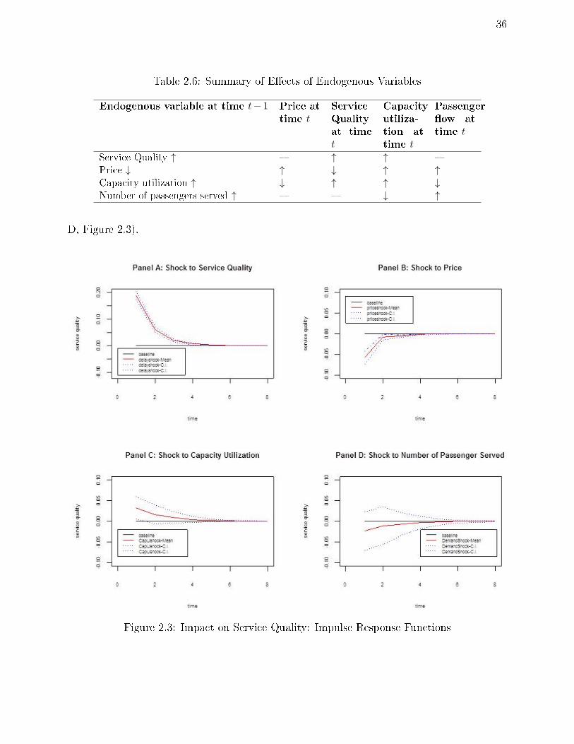
36
Table 2.6: Summary of Eects of Endogenous Variables
Endogenous variable at time t− 1 Price at
time tService
Quality
at time
t
Capacity
utiliza-
tion at
time t
Passenger
ow at
time t
Service Quality ↑ ↑ ↑ Price ↓ ↑ ↓ ↑ ↑Capacity utilization ↑ ↓ ↑ ↑ ↓Number of passengers served ↑ ↓ ↑
D, Figure 2.3).
Figure 2.3: Impact on Service Quality: Impulse Response Functions
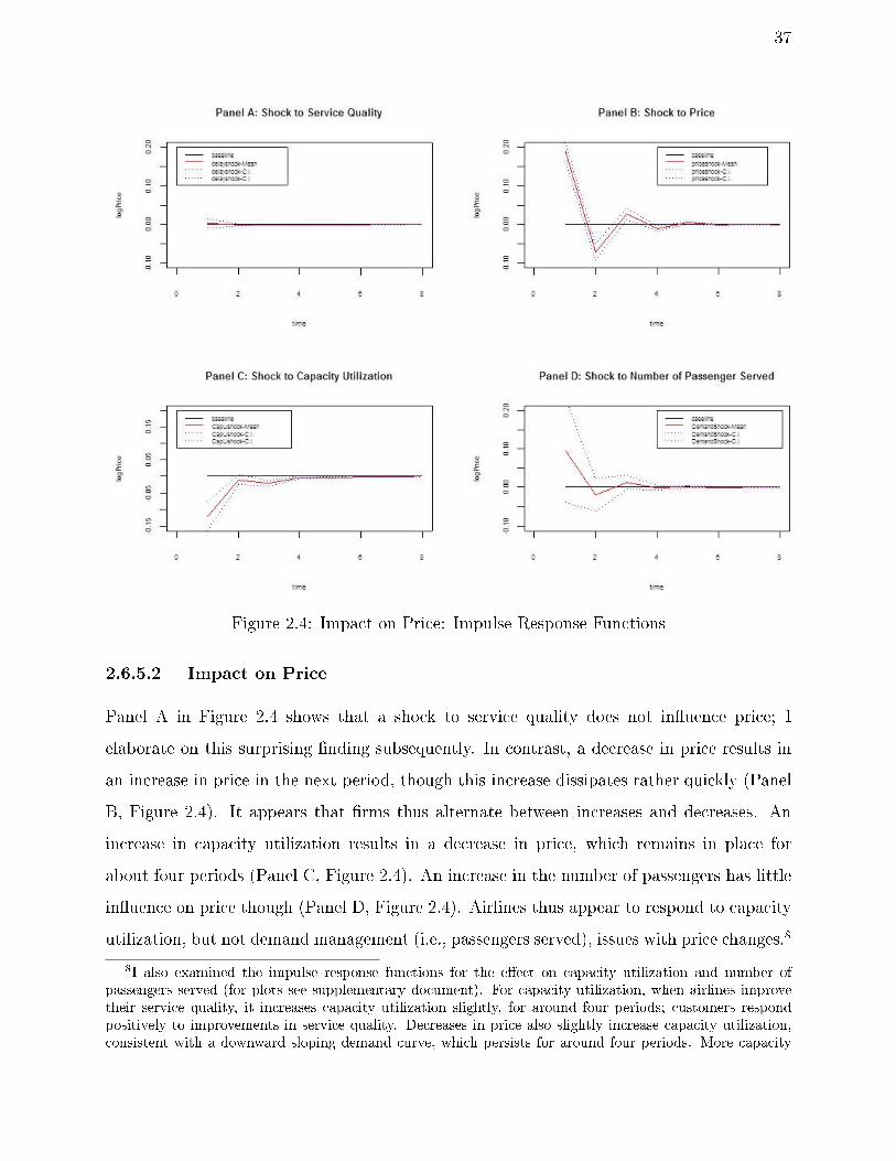
37
Figure 2.4: Impact on Price: Impulse Response Functions
2.6.5.2 Impact on Price
Panel A in Figure 2.4 shows that a shock to service quality does not inuence price; I
elaborate on this surprising nding subsequently. In contrast, a decrease in price results in
an increase in price in the next period, though this increase dissipates rather quickly (Panel
B, Figure 2.4). It appears that rms thus alternate between increases and decreases. An
increase in capacity utilization results in a decrease in price, which remains in place for
about four periods (Panel C, Figure 2.4). An increase in the number of passengers has little
inuence on price though (Panel D, Figure 2.4). Airlines thus appear to respond to capacity
utilization, but not demand management (i.e., passengers served), issues with price changes.8
8I also examined the impulse response functions for the eect on capacity utilization and number ofpassengers served (for plots see supplementary document). For capacity utilization, when airlines improvetheir service quality, it increases capacity utilization slightly, for around four periods; customers respondpositively to improvements in service quality. Decreases in price also slightly increase capacity utilization,consistent with a downward sloping demand curve, which persists for around four periods. More capacity
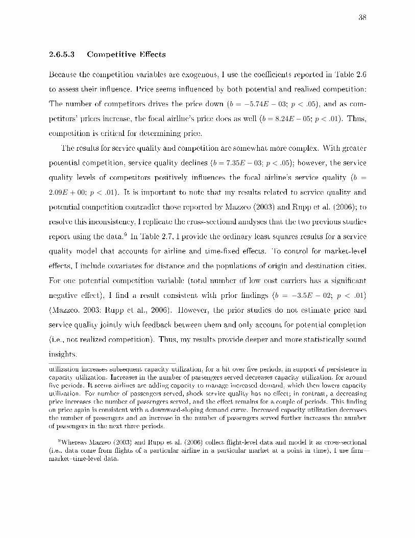
38
2.6.5.3 Competitive Eects
Because the competition variables are exogenous, I use the coecients reported in Table 2.6
to assess their inuence. Price seems inuenced by both potential and realized competition:
The number of competitors drives the price down (b = −5.74E − 03; p < .05), and as com-
petitors' prices increase, the focal airline's price does as well (b = 8.24E − 05; p < .01). Thus,
competition is critical for determining price.
The results for service quality and competition are somewhat more complex. With greater
potential competition, service quality declines (b = 7.35E − 03; p < .05); however, the service
quality levels of competitors positively inuences the focal airline's service quality (b =
2.09E + 00; p < .01). It is important to note that my results related to service quality and
potential competition contradict those reported by Mazzeo (2003) and Rupp et al. (2006); to
resolve this inconsistency, I replicate the cross-sectional analyses that the two previous studies
report using the data.9 In Table 2.7, I provide the ordinary least squares results for a service
quality model that accounts for airline and time-xed eects. To control for market-level
eects, I include covariates for distance and the populations of origin and destination cities.
For one potential competition variable (total number of low cost carriers has a signicant
negative eect), I nd a result consistent with prior ndings (b = −3.5E − 02; p < .01)
(Mazzeo, 2003; Rupp et al., 2006). However, the prior studies do not estimate price and
service quality jointly with feedback between them and only account for potential completion
(i.e., not realized competition). Thus, my results provide deeper and more statistically sound
insights.
utilization increases subsequent capacity utilization, for a bit over ve periods, in support of persistence incapacity utilization. Increases in the number of passengers served decreases capacity utilization, for aroundve periods. It seems airlines are adding capacity to manage increased demand, which then lowers capacityutilization. For number of passengers served, shock service quality has no eect; in contrast, a decreasingprice increases the number of passengers served, and the eect remains for a couple of periods. This ndingon price again is consistent with a downward-sloping demand curve. Increased capacity utilization decreasesthe number of passengers and an increase in the number of passengers served further increases the numberof passengers in the next three periods.
9Whereas Mazzeo (2003) and Rupp et al. (2006) collect ight-level data and model it as cross-sectional(i.e., data come from ights of a particular airline in a particular market at a point in time), I use rmmarkettime-level data.
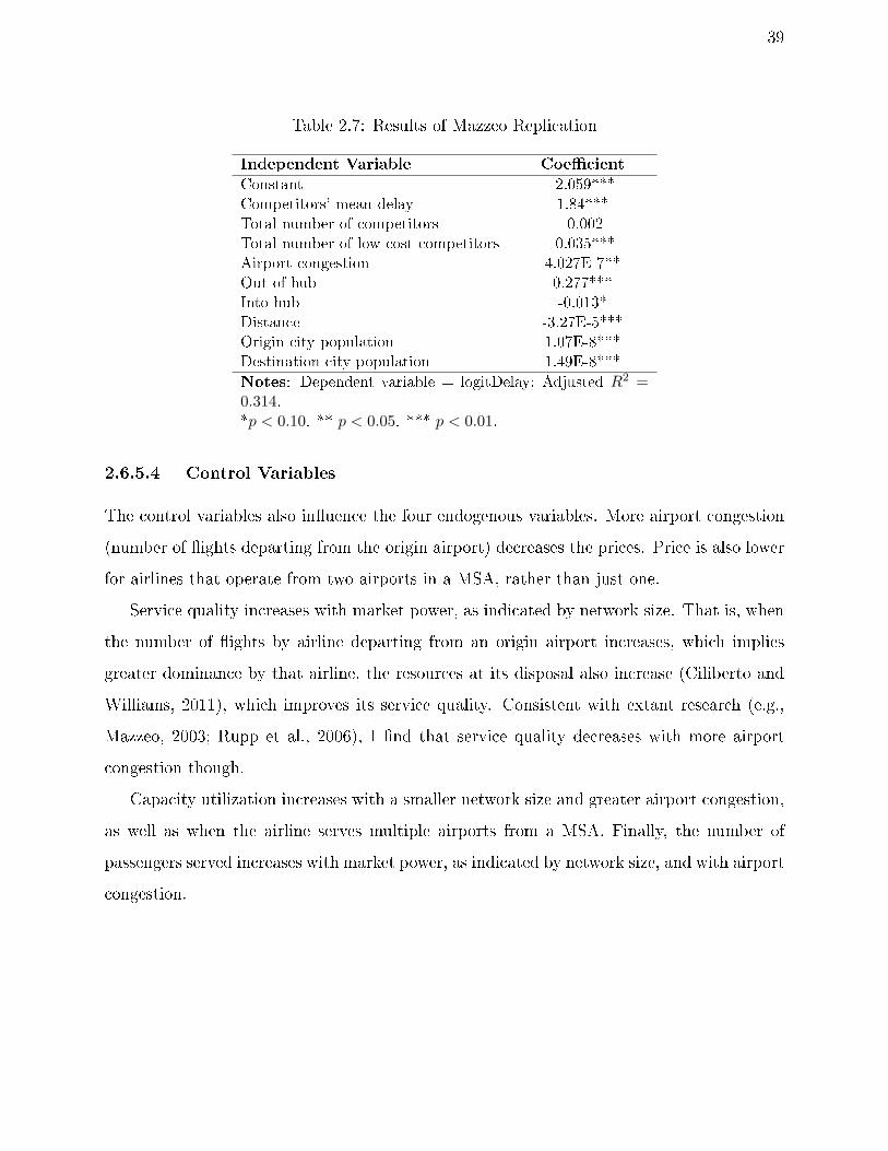
39
Table 2.7: Results of Mazzeo Replication
Independent Variable Coecient
Constant -2.059***Competitors' mean delay 1.84***Total number of competitors -0.002Total number of low cost competitors -0.035***Airport congestion 4.027E-7**Out of hub 0.277***Into hub -0.013*Distance -3.27E-5***Origin city population 1.07E-8***Destination city population 1.49E-8***
Notes: Dependent variable = logitDelay; Adjusted R2 =0.314.*p < 0.10. ** p < 0.05. *** p < 0.01.
2.6.5.4 Control Variables
The control variables also inuence the four endogenous variables. More airport congestion
(number of ights departing from the origin airport) decreases the prices. Price is also lower
for airlines that operate from two airports in a MSA, rather than just one.
Service quality increases with market power, as indicated by network size. That is, when
the number of ights by airline departing from an origin airport increases, which implies
greater dominance by that airline, the resources at its disposal also increase (Ciliberto and
Williams, 2011), which improves its service quality. Consistent with extant research (e.g.,
Mazzeo, 2003; Rupp et al., 2006), I nd that service quality decreases with more airport
congestion though.
Capacity utilization increases with a smaller network size and greater airport congestion,
as well as when the airline serves multiple airports from a MSA. Finally, the number of
passengers served increases with market power, as indicated by network size, and with airport
congestion.

40
2.7. Conclusion
Service quality and price decisions are critical for service rms; I have sought to model
the interplay across these strategic marketing decisions and performance outcomes in the
presence of both realized and potential competition. I gather a unique, multisource data set
pertaining to the airline industry and develop a structural panel VAR model that captures
its idiosyncrasies, such as cross-sectional dependencies and missing observations.
My ndings suggest interesting patterns of asymmetry eects among the endogenous
variables. In particular, I note the asymmetry between service quality and price; though
service quality decisions adjust to price, my results suggest that pricing decisions are not
adjusted to service quality. Together with the result for competition variables, this nding
indicates that rms adjust their prices primarily to manage capacity and in response to
potential and realized competition. Service quality decisions instead reect considerations of
price, performance, and competitive factors. Finally, price exerts more of an impact on the
two performance measures than does service quality; it inuences both capacity utilization
and demand, whereas service quality only aects capacity utilization.
Beyond these unique ndings and the substantive insights they provide into service qual-
ity and pricing decisions in the airline industry, I introduce several unique elements in the
model. To build the model, I explicitly recognized key features of the data, which supported
the three-way structural PVAR, with exogenous competition and control variables. With this
model, I could glean contemporaneous and lagged eects and understand the complexities
inherent in service quality and pricing decisions at the market level for industries in which
rms compete in multiple markets. A clear insight arises with regard to potential competi-
tion for service quality; in contrast with extant cross-sectional studies (Mazzeo, 2003; Rupp
et al., 2006), I nd that greater potential competition (number of competitors) leads to
diminished service quality. If I combine this outcome with the result related to realized com-
petition, I can posit that more competitors deteriorates service quality because it demands
more sharing of resources in the market (e.g., airport facilities), whereas realized competi-
tion positively inuences service quality, as should be expected in a competitive setting. The
panel nature of my model allows for the many cross-sections in the data in terms of rms and
41
markets; the VAR component acknowledges the system of multiple equations that inuence
one another. I also recognize several other complexities in the data, including cross-sectional
dependencies and missing values. My model thus can capture the complexities inherent
in modeling marketing mix variables for dynamic competition among rms across multiple
markets.
Despite these model and estimation complexities, my primary objective has been to pro-
vide insights into the interplay of service quality and pricetwo primary marketing decision
variables for service rmsin the presence of competition. My results provide some key
insights, especially for the airline industry. The extent to which these ndings generalize to
other service industries, such as hotels and banking, should be the topic of further empirical
investigations. I also provide groundwork for additional theoretical models; for example,
new theoretical models might depict the asymmetry between service quality and price, such
that service quality is inuenced by price but price is not inuenced by service quality, to
support decisions about both variables.

Chapter 3
Modeling Service Quality: The Impact of Firm,
Demand, and Competitive Factors
Abstract
Service delivery comprises dierent dimensions based on industrial contextual factors,
such as market characteristics, competitive responses, and rm characteristics that
inuence service quality decisions across these dimensions. In this chapter, I explore how
rms' service quality decisions are inuenced by market and rm characteristics, and
competitors' service quality decisions. I apply the static game framework to account for
the competitive interaction among rms. In the U.S. airline context, the context of my
research, ight cancellations and delays are two critical service quality dimensions that
rms strategically adjust by choosing relevant resource inputs, such as ground support,
eet scheduling, and crew assignment. I develop a static discrete game to model these
two service quality decisions, using data provided by the U.S. Bureau of Transportation
Statistics. In my model, rms rationally anticipate each other's actions and I estimate
rms' service quality choices as a system of simultaneous discrete choice models. The
results show that rms tend to provide high service quality on both dimensions under
the following three conditions: (1) when there are many businesses in the market,
which indicates a strong potential demand from business customers; (2) when rms
have high capacity utilization, which suggests that more ecient capacity management
also leads to better service quality; and (3) when competitors provide low service quality
in one dimension either by having high ight cancellations or high delays, leading to
incentives for rms to provide high service quality in both dimensions to dierentiate
themselves. The results also show that rm-specic factors and competitive responses
have asymmetric impacts on ight cancellation and delay decisions; more specically,
ight cancellation decisions are largely driven by the amount of ight supply and the
42

43
level of capacity utilization, whereas rms respond to competition mainly by adjusting
their average delays. Finally, my model allows me to test two counterfactual situations
of hypothetical absenses of new entrant rms, measure the expected response of the
incumbent competitors, and quantify the impact of the presence of new entrant rm(s)
of various service quality levels on incumbent competitors.
44
3.1. Introduction
In the airline industry, ight on-time performance is a basic but important indicator of
service quality. To most consumers, it is important to safely arrive at the destination on
the scheduled time. Indeed, Bureau of Transportation Statistics (BTS) publishes Air Travel
Consumer Reports yearly to track on-time performances of major rms (airlines). Some
media press and online search engines, such as New York Times and FindTheBest, track and
compare the on-time performances of major rms from time to time, to provide references for
consumers to choose which rm(s) to y with. Though the on-time performance of a rm is
inuenced by uncontrollable factors, such as weather, airport congestion, etc., rms are able
to control their on-time performances to a large extent. For instance, United Airlines started
to oer on-time bonuses to employees since 2008, such that employees are willing to facilitate
the process of transiting aircrafts from serving one ight to another. Southwest Airlines
strategically constrained their aircrafts to a limited set of models to reduce the burden of
aircrafts and crews scheduling/rescheduling. Many rms, such as KLM, Air France and
Eagles Air, implemented specic programs for aircrafts maintenance and ground support
sta training, to prepare aircrafts for the next scheduled ight eciently.
It is important for rms to provide good on-time performance, and it seems feasible for
them to improve it. We then may expect most rms to have good on-time records. However,
this inference does not seem to be true. The Air Travel Consumer Reports show that from
2009 to 2010, Delta Airlines had 17.5% of ights delayed and JetBlue had 23.8% of ights
delayed. It shows that some major rms do provide substantial amount of delayed ight
services, despite the importance of on-time performance. As discussed above, rms are able
to allocate resources to improve their on-time performance. The numbers reported in the
Air Travel Consumer Reports suggest that some major rms choose not to allocate sucient
resources to ight on-time performance.
If we compare the on-time performances of rms in dierent markets, we may nd that
they dier substantially across rms and markets. For example, in the third quarter of 2010,
American Airlines had 44% of ights delayed for more than 15 minutes in the Los Angeles-
Denver market; in comparison, Southwest Airlines had a much better performance with
45
only 28% of ights delayed in that market (Figure 3.1). In the market St. Louis-Seattle,
for the same quarter, the situation was reversed, with American Airlines having 26% of
ights delayed and Southwest having 36% of ights delayed. The ip in relative on-time
performance in these two markets seems to suggest that rms strategically allocate dierent
levels of service-related resources in dierent markets.
Firms' decisions on service related allocation frequently involve a trade-o between re-
ducing costs and increasing quality dimensions (Anderson, Fornell and Rust, 1997; Rust,
Moorman and Dickson, 2002). Managers must decide not only how to allocate resources to
service quality versus other aspects of the business (e.g., improving productivity) but also
how to allocate the service pool of resources across dierent markets. These decisions may be
largely inuenced by resource requirements to improve service quality, the impact of service
quality on demand, and how competitors' service quality is likely to change in response to
the focal rm's actions.
This paper aims at explaining rms' decisions on service quality by disentangling three
groups of driving factors, which I refer to as rm characteristics, market characteristics, and
competitive factors, and quantifying the impact of each factor on the service quality decision.
I use the airline industry of the United States as my research context. In the airline industry,
the core service is the journey (i.e., transport passengers from city A to city B). Passengers
usually expect to arrive at their destinations on time; however, it is not uncommon that
ights are cancelled or delayed (Mazzeo, 2003; Rupp and Holmes, 2006). I thus use both
ight cancellation rate and ight delay rate of a rm in a market, which I dene as a route
(e.g., Atlanta-Los Angeles), to represent the rm's service quality level in the market. In
addition, to account for the competitive interaction among rms, I propose a static discrete
game (other examples of similar approaches included Bajari, Hong, Krainer and Nekipelov
(2005) and Ellickson and Misra (2008)), in which service quality choice is dened as a unique
combination of cancellation and delay level.
I use data from the airline industry in the United States to estimate the model. I nd
that rms tend to provide high service quality on both dimensions under the following three
conditions: (1) when there are many businesses in the market, which indicates a strong
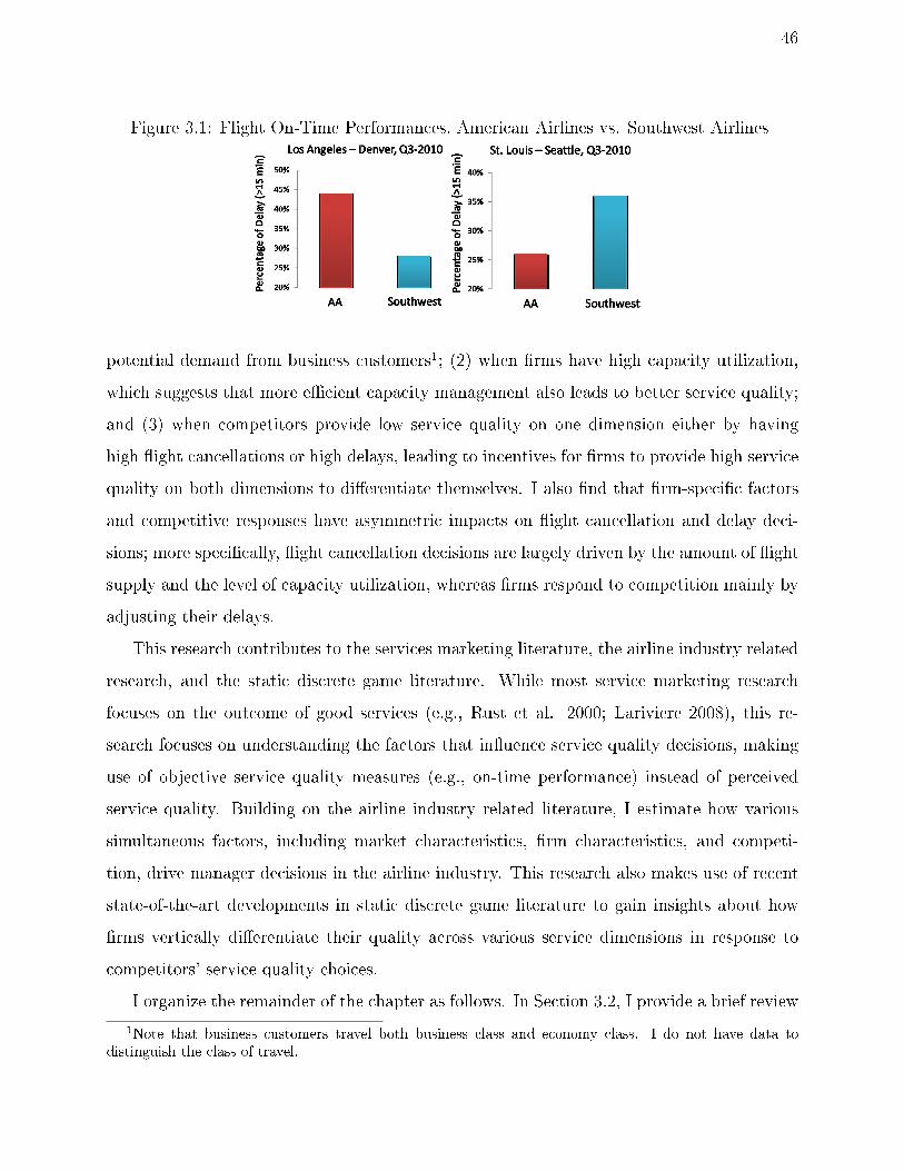
46
Figure 3.1: Flight On-Time Performances, American Airlines vs. Southwest Airlines
potential demand from business customers1; (2) when rms have high capacity utilization,
which suggests that more ecient capacity management also leads to better service quality;
and (3) when competitors provide low service quality on one dimension either by having
high ight cancellations or high delays, leading to incentives for rms to provide high service
quality on both dimensions to dierentiate themselves. I also nd that rm-specic factors
and competitive responses have asymmetric impacts on ight cancellation and delay deci-
sions; more specically, ight cancellation decisions are largely driven by the amount of ight
supply and the level of capacity utilization, whereas rms respond to competition mainly by
adjusting their delays.
This research contributes to the services marketing literature, the airline industry related
research, and the static discrete game literature. While most service marketing research
focuses on the outcome of good services (e.g., Rust et al. 2000; Lariviere 2008), this re-
search focuses on understanding the factors that inuence service quality decisions, making
use of objective service quality measures (e.g., on-time performance) instead of perceived
service quality. Building on the airline industry related literature, I estimate how various
simultaneous factors, including market characteristics, rm characteristics, and competi-
tion, drive manager decisions in the airline industry. This research also makes use of recent
state-of-the-art developments in static discrete game literature to gain insights about how
rms vertically dierentiate their quality across various service dimensions in response to
competitors' service quality choices.
I organize the remainder of the chapter as follows. In Section 3.2, I provide a brief review
1Note that business customers travel both business class and economy class. I do not have data todistinguish the class of travel.
47
of the service marketing literature and the static discrete game literature. In Section 3.3, I
provide the background information about how ight cancellations and delays happen. In
Section 3.4, I describe my data set and relevant variables. After specifying the model in
Section 3.5. I present the estimation details and identication strategy in Section 3.6. The
main results, a discussion of their implications, and robustness checks appear in Section
3.7. I conduct counterfactual analyses to measure the impact of new entrants on incumbents
service quality decisions in Section 3.8. Finally, in Section 3.9, I discuss the insights generated
from these results and conclude the paper with managerial implications and directions for
future research.
3.2. Literature Review
This research pertains to the service marketing literature, in which service quality is reected
by some measurable combination of tangibility, reliability, responsiveness, assurance, and
empathy (Parasuraman, Berry and Zeithaml, 1985; Parasuraman et al., 1988; Parasuraman
et al., 1991). Various studies establish positive outcomes of improved service quality, such as
greater customer satisfaction and retention (e.g., Lariviere, 2008; Spreng and Mackoy, 1996;
Zeithaml et al., 1996), increased market share (Rust et al., 2000), and higher shareholder
value (Grewal et al., 2010). Other research distinguishes how customer satisfaction can be
inuenced by service quality at each stage of the service delivery process (e.g., Danaher and
Mattsson, 1994; de Ruyter, Wetzels, Lemmink and Mattsson, 1997). A few studies also
discuss how rms improve service quality by being market oriented (Raju and Lonial, 2001),
formalizing the selling process, and/or applying a cross-functional team structure (Froehle
et al., 2000). Previous applications generally measure service quality using consumer surveys
(e.g., Lariviere, 2008; Raju and Lonial, 2001) that capture perceived instead of actual service
quality. This research adds to this literature by focusing on understanding the factors that
inuence service quality decisions, making use of objective service quality measures (e.g.,
on-time performance) instead of perceived service quality.
This research is also related to past literature on the airline industry. In this area, previous
work have established that perceived service quality enhances customer loyalty (Zins, 2001),
48
whereas poor service quality negatively moderates the positive eects of aircraft productivity
on return on assets and sales (Sim, Koh and Shetty, 2006). Jou, Lam, Hensher, Chen and
Kuo (2008) estimate a static demand-cost equilibrium, and shows that safety, convenience,
and service quality (based on customer satisfaction surveys) increase demand. Some studies
specically explore the on-time performance of airlines and show that delay and cancellation
performances are interdependent across airlines (Ball, Homan, Chen and Vossen, 2000)
and that airlines have relatively lower delay and cancellation rates when competition is
more severe compared with when competition is mild (Mazzeo, 2003; Rupp and Holmes,
2006; Rupp et al., 2006). Furthermore, studies in other industries assess how rms choose
quality levels (e.g., motel vs. hotel; self-service vs. full-service), jointly with market entry
and location decisions (Hastings, 2004; Iyer and Seetharaman, 2005; Mazzeo, 2002). To
contribute to this literature, I estimate how various simultaneous factors, including market
characteristics, rm characteristics, and competition, drive manager decisions in the airline
industry.
The estimation technique used in this paper stems from economics and marketing re-
search on static discrete game estimation. Similar estimations have addressed research prob-
lems related to market entry and location choices (e.g., Vitorino, 2012; Zhu, Singh and
Dukes, 2011), retailer pricing strategies (Ellickson and Misra, 2008), and group purchase
decisions (Hartmann, 2010). The key feature of these research problems is that the decision
maker chooses an action from an action set, taking into consideration the choices of other
decision makers (e.g., competitor, peer consumer). I make use of these recent state-of-the-art
developments in models of the supply side to gain insights about the actions of rms and
how the competitive environment aects the service quality levels in the airline industry.
3.3. Background Information: On-Time Performance in
Airline Industry
Flight cancellation and ight delay may be caused by many factors. Some of these factors
can not be controlled by rms, such as bad weather, airport congestion, and national secu-

49
rity concerns. However, according to statistics provided by BTS (Bureau of Transportation
Statistics), around 60% of ight cancellations and delays are caused by controllable reasons,
such as mechanical problems, shortage of gate slots, crew out-of-time and late aircraft ar-
rivals. All of these reasons are closely related to a tradeo rms constantly face - improving
on-time performance and service quality vs. reducing cost of operational resources.
A rm's main operational resources in the airline industry include assigned gate and
runway slots in each airport, aircrafts, and crews. A rm's gate and runway slots in each
airport are assigned by FAA (Federal Aviation Association) at a semi-yearly or yearly base,
and thus are limited resources. Aircrafts are costly to purchase, lease or maintain. Crew
salaries and benets also cost rms a substantial amount of money. In addition, there
are strict rules about the maximal amount of time a crew, especially a pilot can serve
daily, as well as the minimal number of breaks a crew should have monthly. Due to the
substantial amount of costs of adding additional aircrafts and crews, rms tend to maximize
their aircraft and crew utilization, which means, to let aircrafts and crews serve as many
ights as possible. Given the limited number of assigned gate and runway slots, aircrafts,
and crews rms implement complicated algorithms to route their aircrafts and crews in a
way that maximally satises the ight service needs and in the meanwhile minimizes costs.
The routing plans suggested by algorithms work well at ideal conditions, that is, when
there are no interruptions from the runway/gate congestion, crew sickness/strikes, aircraft
wear-outs, etc. In reality, however, these interruptions often happen. For example, the line
of ights awaiting to take o is longer than expected, and in the meanwhile, one of the pilots
runs out of the allowed service time and is forced to stop his/her duty if the ight has not
taken o. Under this circumstance, if there is no back-up pilot arriving on time, the ight
has to be delayed or cancelled. If a crew is sick when s/he is about to serve a ight duty and
there are no backup crews arriving on time, the ight is likely to be delayed or cancelled.
Similarly, if the aircraft happens to have mechanical problems before taking o, and the
rm cannot assign a back-up aircraft on time, the ight will be delayed or even cancelled.
It seems that backup crews and aircrafts may solve these problems in most cases, but these
resources are costly, and rms usually cannot aord the luxury of having sucient backup
resources. In addition, we may wonder that if rms do regular mechanical inspections during

50
breaks of aircrafts ight services, they may avoid most of the mechanical problems before
aircrafts take o. But the problem is rms tend to y their aircrafts as much as they can to
save costs, so it is not feasible to provide the regular mechanical inspection to every aircraft
during its service breaks.
The scenarios described above are common issues that cause ight cancellations and ight
delays. However, if we take into consideration the aircraft and crew routing dynamics, we
may see more issues leading to ight cancellations and delays. With the limited number of
gate slots, rms tend to schedule as many ights departing from and arriving at a gate as
possible. It implies that to ensure perfect on-time performance, all ights scheduled to depart
from (arrive at) a gate have to depart (arrive) on-time. If any of the scenarios described
above happens, the delayed/cancelled ight will take the gate longer than it should, causing
delays of the next scheduled ight to depart from (arrive at) the focal gate. The dynamic
aircraft and crew routing also cause potential carry over delays. If a ight is delayed, the
aircraft and crews cannot arrive at the destination airport to start the next assigned ight
duty, causing delays of the next scheduled ight, and likely delays of the scheduled ight
after next. If a rm does not have backup aircrafts and crews to substitute the subsequent
scheduled ight duties, one ight delay may cause a sequence of ight delays. This type of
delay is named as the late aircraft arrival delay.
When rms encounter unexpected disruptions, and they do not have sucient backup
resources to keep all the scheduled ights on time, they face two choices: to keep the original
schedule and delay ights that are subject to the disruptions, or to cancel some ights.
These two options each has pros and cons. Delaying ights keeps the scheduled service
commitments and does not cause operational burden of rescheduling aircrafts, crews, and
passengers, but it may cause carry over delays of subsequent ights (in the same market, or
in other markets). Cancelling ights instead, gains the rm sucient resources (e.g., gate
slots, spare aircraft and crews) to keep subsequent ights (in the same market, or in other
markets) on time, but it harms the brand image among passengers, as it implies breaking
service commitment.
Overall, rms often face the following tradeos: to have sucient backup resources for
unexpected disruptions so as to keep good on-time records, or to save costs by fully utilizing

51
all the available resources; and once they are vulnerable to unexpected disruptions, they will
have to decide between cancelling ights and delaying ights. The benets and costs of each
option, are inuenced by market and rm characteristics, as well as competitors' on-time
performance.
3.4. Data
3.4.1 Data Description
I collect my data from two sources: the Bureau of Transportation Statistics (BTS) and
U.S. Census Bureau. I gather data on delays and cancellations of ights from the On-
Time Performance BTS data set. This data set indicates departure delays, measured as the
dierence in minutes between scheduled and actual departure time; arrival delays, or the
dierence in minutes between the scheduled and actual arrival time; and cancellations, i.e.,
whether the ight is cancelled or not. The data are available for each domestic ight operated
by rms that earn at least 1% of the total revenue in the airline industry. The cancellation
measurement is directly taken from BTS data; consistent with previous literature (e.g.,
Mazzeo, 2003; Rupp et al., 2006), we use arrival delays to measure on-time performances,
because passengers are likely to care more about arrival delay than departure delay.
The T100 Origin and Destination database from the BTS provides additional relevant
information for the analysis. This census dataset describes trac for all domestic origins
and destinations by rms with annual revenues greater than $20 million. The included
variables are: total passengers served, total number of seats provided, total number of ight
departures performed, total number of ight departures scheduled, and distance for each
market (route), where a market (route) is a unique origin-destination combination (e.g.,
Berry and Jia, 2010). I use the total number of ight departures performed and capacity
utilization (total number of passengers served/total number of seats provided) to partially
determine the rm characteristics. For the market characteristics data (e.g., number of
business, income per capita), I turn to the U.S. Census Bureau.
Although BTS maintains data on all 25163 U.S. routes, I restrict the analysis to routes
52
that satisfy the following criteria: (1) market share larger than 60% for four major airlines
(American Airlines, Delta Airlines, United Airlines, Southwest Airlines); (2) the majority
of passengers (i.e., greater than 60%) take a direct ight, so that passenger choices are less
aected by connecting ights; (3) there is only one major airport in the origin/destination
city, to avoid potential airport level competition; and (4) the distance between the origin
city and the destination city is greater than 600 miles, to avoid the potential competition
from other means of transportation (i.e., car, train, bus). The nal sample includes 15 cities,
112 routes, 4 rms, and 71 quarters. The time frame goes from quarter 2 of 1993 to quarter
4 of 2010, producing 9,819 observations in all.
3.4.2 Examples of Service Quality Variation
I select two representative markets (Atlanta-San Francisco and Los Angeles-Denver) to reveal
some interesting patterns in the data about the two service quality dimensions, ight delays
and cancellations. The rst (upper) plot in Figure 3.2 shows the performance of the two
major rms, Delta and United, in the Atlanta-San Francisco market. The gure reveals that
Delta Airlines had longer average ight delays than United Airlines for all the time under
analysis, although after 2004, the dierences between the delays of these two rms became
smaller. The rst (upper) plot in Figure 3.3 shows the rates of ight cancellations for the two
rms in the same market. In this case, United Airlines had more frequent ight cancellations
than Delta Airlines, and the dierences became more apparent after 2004. These patterns
suggest that United decreased its level of service quality in this route after 2004, and my
model aims at explaining these patterns with changes in market conditions and rm factors.
The Los Angeles-Denver market (see second plots in Figure 3.2 and Figure 3.3) presents a
unique situation that is somewhat common in the dataset. United Airlines held a monopoly
before 2000 until the entry of American Airlines. When American Airlines entered, United
reduced its average delay minutes and cancellation rate over 2000 and 2001. In 2008, South-
west Airlines also entered this market. We observe that both United Airlines and American
Airlines decreased their average delay minutes at the time of the entry, suggesting some
competitive response to the presence of the new entrant. The model I propose takes into
account the possibility of competitive reactions to explain the levels of service quality.
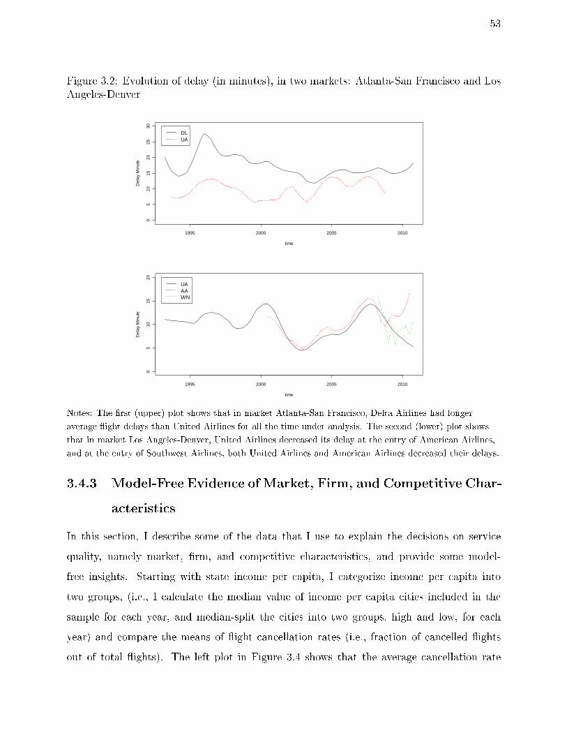
53
Figure 3.2: Evolution of delay (in minutes), in two markets: Atlanta-San Francisco and LosAngeles-Denver
1995 2000 2005 2010
05
1015
2025
30
time
Del
ay M
inut
eDLUA
1995 2000 2005 2010
05
1015
20
time
Del
ay M
inut
e
UAAAWN
Notes: The rst (upper) plot shows that in market Atlanta-San Francisco, Delta Airlines had longer
average ight delays than United Airlines for all the time under analysis. The second (lower) plot shows
that in market Los Angeles-Denver, United Airlines decreased its delay at the entry of American Airlines,
and at the entry of Southwest Airlines, both United Airlines and American Airlines decreased their delays.
3.4.3 Model-Free Evidence of Market, Firm, and Competitive Char-
acteristics
In this section, I describe some of the data that I use to explain the decisions on service
quality, namely market, rm, and competitive characteristics, and provide some model-
free insights. Starting with state income per capita, I categorize income per capita into
two groups, (i.e., I calculate the median value of income per capita cities included in the
sample for each year, and median-split the cities into two groups, high and low, for each
year) and compare the means of ight cancellation rates (i.e., fraction of cancelled ights
out of total ights). The left plot in Figure 3.4 shows that the average cancellation rate

54
Figure 3.3: Evolution of cancellation rate (in fraction of total ights), in two markets:Atlanta-San Francisco and Los Angeles-Denver
1995 2000 2005 2010
0.00
0.01
0.02
0.03
0.04
0.05
time
Can
cella
tion
Fra
ctio
nDLUA
1995 2000 2005 2010
0.00
0.01
0.02
0.03
0.04
0.05
0.06
time
Can
cella
tion
Fra
ctio
n
UAAAWN
Note: The rst (upper) plot shows that in market Atlanta-San Francisco, United Airlines had more
frequent ight cancellations than Delta Airlines, and the dierences got more apparent after 2004. The
second (lower) plot shows that in market Los Angeles-Denver, United Airlines decreased its cancellation
rates after the entry of American Airlines, and before the entry of Southwest Airlines, both United Airlines
and American Airlines decreased their cancellation rates.
is higher in markets with high state income per capita than in the low state income per
capita group, which oers a counter intuitive pattern. We would expect instead that rms
provide better services in markets with high income per capita. However, if we take a close
look at the cities with low and high state income per capita, we can better understand the
pattern. Several cities with low income per capita (at the state level), including Atlanta,
Dallas, St. Louis, Phoenix, Miami, and Tampa, are busier, larger, and more complex air
transportation centers, where ight cancellations may lead to very negative impacts due to
the large volume of passengers, ights, and connections to be handled. Additionally, these
are also cities located in the south of the United States, where the weather is rarely the cause
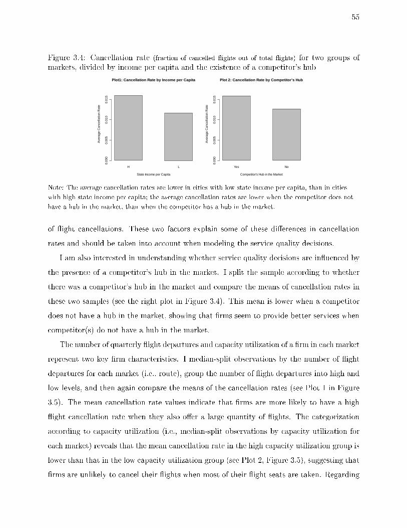
55
Figure 3.4: Cancellation rate (fraction of cancelled ights out of total ights) for two groups ofmarkets, divided by income per capita and the existence of a competitor's hub
H L
Plot1: Cancellation Rate by Income per Capita
State Income per Capita
Ave
rage
Can
cella
tion
Rat
e
0.00
00.
005
0.01
00.
015
Yes No
Plot 2: Cancellation Rate by Competitor's Hub
Competitor's Hub in the Market
Ave
rage
Can
cella
tion
Rat
e
0.00
00.
005
0.01
00.
015
Note: The average cancellation rates are lower in cities with low state income per capita, than in cities
with high state income per capita; the average cancellation rates are lower when the competitor does not
have a hub in the market, than when the competitor has a hub in the market.
of ight cancellations. These two factors explain some of these dierences in cancellation
rates and should be taken into account when modeling the service quality decisions.
I am also interested in understanding whether service quality decisions are inuenced by
the presence of a competitor's hub in the market. I split the sample according to whether
there was a competitor's hub in the market and compare the means of cancellation rates in
these two samples (see the right plot in Figure 3.4). This mean is lower when a competitor
does not have a hub in the market, showing that rms seem to provide better services when
competitor(s) do not have a hub in the market.
The number of quarterly ight departures and capacity utilization of a rm in each market
represent two key rm characteristics. I median-split observations by the number of ight
departures for each market (i.e., route), group the number of ight departures into high and
low levels, and then again compare the means of the cancellation rates (see Plot 1 in Figure
3.5). The mean cancellation rate values indicate that rms are more likely to have a high
ight cancellation rate when they also oer a large quantity of ights. The categorization
according to capacity utilization (i.e., median-split observations by capacity utilization for
each market) reveals that the mean cancellation rate in the high capacity utilization group is
lower than that in the low capacity utilization group (see Plot 2, Figure 3.5), suggesting that
rms are unlikely to cancel their ights when most of their ight seats are taken. Regarding

56
Figure 3.5: Cancellation rate for two group of rms based on rm characteristics: numberof departures performed, capacity utilization, and hub destination.
H L
Plot 1: Cancellation Rate by Departure Performed
Departure Performed
Ave
rage
Can
cella
tion
Rat
e
0.00
00.
005
0.01
00.
015
H L
Plot 2: Cancellation Rate by Capacity Utilization
Capacity Utilization
Ave
rage
Can
cella
tion
Rat
e
0.00
00.
005
0.01
00.
015
Yes No
Plot3: Cancellation Rate by Hub Destination
Destination is a Hub
Ave
rage
Can
cella
tion
Rat
e
0.00
00.
005
0.01
00.
015
Note: The average cancellation rates are lower when the number of quarterly ight departures are low than
when the number of ight departures are high; the average cancellation rates are lower when the capacity
utilization is low than when the capacity utilization is high; the average cancellation rates are lower when
the destination airport is not a hub than when the destination airport is a hub.
the existence of own hub, Plot 3 in Figure 3.5 suggests that mean of cancellation rate is
higher when the destination is a rm's own hub, compared to when the destination is not a
hub.
As an example of competitive response, I use the Los Angeles-Denver market, where
incumbent(s) seemed to react to a new entrant by adjusting their service quality levels. I
compare the changes in average delay (in minute) and cancellation rates across a group of
markets with and without Southwest. Southwest entered the Boston-Denver market in the
rst quarter of 2010 but was not present in some other markets originating from Boston. I
compute the mean average delay and mean cancellation rates of incumbent rms before and
after the entry of Southwest in the Boston-Denver market against those of the incumbent
rms before and after the rst quarter of 2010 (when Southwest entered the Boston-Denver
market) for other markets that originated in Boston without the presence of Southwest (see
Figure 3.6). With the presence of Southwest, I observe that the mean average delays and
cancellation rates declined more in the Boston-Denver market than in markets in which
Southwest never entered.
I provide descriptive statistics about the measurements of service quality and the inde-
pendent variables in Table 3.1. The average ight cancellation rate was 1.4%, while the

57
Figure 3.6: Incumbents' Service Quality Reaction to Southwest Entry: Origin Boston
Before After
Incumbents' Delay (in Minute): Boston-Denver
Southwest Entry
Ave
rage
Del
ay M
inut
e
02
46
810
12
Before After
Incumbents' Cancellation Rate: Boston-Denver
Southwest Entry
Ave
rage
Can
cella
tion
Rat
e
0.00
00.
005
0.01
00.
015
Before After
Delay (in Minute) in Markets without Southwest
Year 2010
Ave
rage
Del
ay M
inut
e
02
46
810
12
Before After
Cancellation Rate in Markets without Southwest
Year 2010
Ave
rage
Can
cella
tion
Rat
e
0.00
00.
005
0.01
00.
015
0.02
0
Note: Incumbent rms' average delay and cancellation rates drop more after the rst quarter of 2010
(when Southwest entered the market Boston-Denver) in Boston-Denver, than in other markets where
Southwest never entered.
average delay was 11.8 minutes, with a large dispersion across markets, rms, and time. In
the analysis, I use the median-centered values of ight cancellation rate and average delay
for each market to capture the relative performance of each rm and control for weather
and location of market that might aect the absolute level of service quality. The markets
included in the data also exhibit large variation in terms of the number of businesses and
income per capita. These variations may be due to market dierences, economic growth
and ination over time. I use the yearly median-centered values of number of businesses and
income per capita in discretization and estimations to account for economic growth/ination
over time.

58
Table 3.1: Descriptive Statistics
Variable Mean Std. Dev. Min Max
Service Quality
Average Flight Delay (minute) 11.84 5.27 0.45 55.16Average Flight cancellation Rate (percentage) 1.4% 1.8% 0% 21.5%Market Characteristics
Number of Businesses (geometric mean of theorigin and destination cities)
87,512 28,052 46,363 181,246
Income per Capita (geometric mean of the ori-gin and destination states)
32,657 6,904 1,885 47,886
Presence of Competitor's hub in the market 0.47 0.50 0 1Firm Characteristics
Total Number of Flight Departures 457.59 332.40 30 1,827Average Capacity Utilization (percentage) 0.74 0.11 0.30 0.97Whether the Origin City is a Hub of the FocalFirm
0.48 0.50 0 1
Whether the Destination City is a Hub of theFocal Firm
0.48 0.50 0 1
3.5. Model
3.5.1 Justication for Assumptions
The delay and cancellation levels of each rm in each market are closely related to the
rm's ight scheduling decisions, which involve eet assignments, block time scheduling, crew
assignments, and so on, coordinated over all markets (i.e., routes) in the rm's ight network.
Flight scheduling is a complex optimization problem, solved by algorithms (e.g. Sohoni,
Lee and Klabjan, 2008), but in practice, rms strategically apply the results generated by
algorithms and decide how much resources (i.e., the length of block time, the number of crew
assigned) to allocate to each market (e.g. Gopalakrishnan and Johnson, 2005), based on the
market conditions and competitive intensity. With this model, I aim to infer how dierent
factors drive rms' strategic decisions on ight cancellation rates and average ight delays
in each market. Firms focus mainly on the total prots from their route networks when
scheduling ights, however, they may still try to extract the most prots from each large
market (i.e., route) they serve. All markets (i.e., routes) in the data set are large markets,
I therefore consider it proper to assume that rms make service quality decisions in each
market to maximize their market prots. Many rms also adjust the block time, eet and
59
crew assignments seasonally (i.e., 2-3 months) (Centeno and Vitt, 2011; Sinnott, 2002), thus,
I model rms' service quality as a quarterly decision.
My goal is to explain the decisions rms make regarding their service quality across
multiple markets. The choice of service quality can be framed as a game among a nite set of
players. Given the competitive environment of the industry, the prots of each rm depend
on the actions of other rms, which are taken into consideration when making decisions.
Therefore, I assume that each rm chooses the service quality that maximizes its expected
prots in each market in each quarter2.
I do not have precise revenue/market share measurements for each rm in each market
at each quarter. Thus, consistent with previous literature (e.g., Berry, 1992; Mazzeo, 2002)
I need to use demand and cost shifters to approximate a reduced form specication of
prots. Market characteristics (i.e., potential demand) are likely to shift the demand, rm
characteristics (i.e., capacity utilization) are likely to drive the cost of each service quality
action, and rm's expectations of competitors' actions may also inuence the prots of
each service quality action. I therefore use these variables related to these three factors to
represent prots.
3.5.2 Intuitions Behind the Model
Each rm chooses a service quality level that maximizes its prots in a market at a time.
As explained in the last paragraph in section 3.4.1, the focal rm's prots of choosing a
service quality level depend on market characteristics, rm characteristics, and competitors'
actions. In addition, some random elements, such as the mechanical problems of airplane
engines, the relationship between the focal rm and its labor union, may also inuence the
prots. If the random elements are drawn from a known distribution, the probability of the
focal rm choosing each service quality level can be computed.
In each time period, rms in the same market choose service quality levels simultaneously.
2Note that I model rms' choice of service quality as a static game. I am aware that service qualitydecisions may have long-term impacts. However, from conversations with airline executives, we realizedthat rms in general only consider short-term prots (recent quarter or semi-year) when making strategicdecisions, because their operational resources (i.e., runway slots, airport gates) assigned by Federal AviationAssociation (FAA) change at a semi-year base, making long-term planning dicult. I believe a static modelis good representation to capture how decisions are made in the industry.

60
That is to say, the focal rm is not able to see the service quality levels its competitors choose
when it makes its own service quality decision . As a result, the focal rm makes a rational
inference (i.e., a belief) about competitors' choices. The focal rm is unlikely to observe
its competitors' random elements; therefore, the focal rm can only have beliefs about the
service quality choice probabilities of its competitors.
If all rms make rational inferences about their competitors' service quality choices (i.e.,
an equilibrium condition is achieved), the expected choice probabilities of competitors, which
enter the focal rm's prot functions, have to be consistent with the competitors' actual
choice probabilities; and competitors' actual choice probabilities are also functions of the focal
rm's choice probabilities. The competition component in the prot function is therefore
endogenous. To address the endogeneity of expected competitors' service quality choices,
and to account for rms' rational expectations about each other's service quality choices, I
need to estimate rms' service quality choices as a system of simultaneous discrete choice
models.
3.5.3 Formal Specication of the Model
I observe rms f = 1, 2..., F serving markets m = 1, 2, ...,M at time t = 1, 2, ..., T . A rm's
service quality choice for market m at time t is denoted as afmt, which can take any discrete
level in the action set k = 1, ...,K. The competitors' service quality actions are denoted
a−fmt = (a1mt, ..., a(f−1)mt, a(f+1)mt, ...aFmt).
Each rm makes a service quality decision in each market it serves, maximizing its local
(market) prots
πfmt = Πfmt(sfmt, afmt, a−fmt) + ϵfmt, (3.1)
where Πfmt is a known and deterministic function of the state vector sfmt dened below,
the focal rm's action afmt, and the competitors' actions a−fmt. The term ϵfmt denotes a
private shock that aects the prots of rm f in market m at time t. As ϵfmt is private
information for each rm, each rm makes decisions based on its own state vector, sfmt,
its competitors' state vectors, s−fmt, its own private shock, ϵfmt, but not its competitors'
private shock ϵ−fmt. Thus, I dene each rm's decision rule as afmt = dfmt(sfmt, s−fmt, ϵfmt),

61
where choices are a function of the state vectors and its own shock, but not the shocks of the
competitors. Without knowing the exact value of each rm's private shock, what a rm (or
an econometrician) can infer about other rms are their probabilities of taking each action,
which depend on the state vectors and the distribution of the private shocks. That is to say,
from both the rms' and the econometrician's perspective, the probability that a given rm
chooses action a, conditional on the state vectors, is
Pr(afmt = a|sfmt, s−fmt) =
∫1dfmt(sfmt, s−fmt, ϵfmt) = af(ϵfmt)dϵfmt, (3.2)
where 1dfmt(sfmt, s−fmt, ϵfmt) = a is an indicator function equal to 1 if rm f in market
m at time t chooses action a and 0 otherwise. Let Pmt denote the set of these probabilities
of all rms in market m at time t and all choice alternatives. Note that the focal rm's
payos from taking each action depends on competitors' actions, but all what the focal
rm knows about competitors are their probabilities of taking each action. The focal rm's
expected payos therefore depend on three components: the deterministic function of the
state vector, Πfmt(sfmt, afmt, a−fmt), the probability of each competitor taking each action,
Pr(a−fmt = a|s−fmt, sfmt), and the private shock, ϵfmt(a). Mathematically, the expected
prots for rm f if it chooses action a in market m at time t (taking the inuence from
competitors' actions into account) is given by
E[πfmt(afmt, sfmt, ϵfmt,Pmt)] = E[πfmt(afmt, sfmt, s−fmt)] + ϵfmt(a) =
=∑
a−fmtΠfmt(sfmt, afmt, a−fmt)P−fmt + ϵfmt(a)
, (3.3)
where P−fmt =∏
jmt =fmt Pr(ajmt | sjmt, s−jmt). Note that P−fmt =∏
jmt =fmt Pr(ajmt |
sjmt, s−jmt) is the products of each competitor's probability of taking each action (in case
there are multiple competitors in the market), and that the term∑
a−fmtΠfmt(sfmt, afmt, a−fmt)P−fmt
is the expected value of Πfmt(sfmt, afmt, a−fmt), marginalizing out the action probabilities of
competitors using P−fmt. Firms choose service quality actions that maximize the expected
prots, thus the probability of rm f taking action a in market m at time t is
Ψfmta = Pr
(E[πfmt(a, sfmt)] + ϵfmt(a) > E[πfmt(a
′, sfmt)] + ϵfmt(a′), ∀a′ = a
), (3.4)

62
which is the system of equations that dene the Bayesian Nash Equilibrium of the game.
I now specify the functional form of the expected prot functions of rm f when it
chooses service quality k in market m at time t. I select three components, related to market
characteristics, rm characteristics, and competitive responses. Competitive responses are
captured by the expected proportion of competitors choosing each service quality strategy,
because the rm should be more worried about how likely each service quality decision
is chosen by its competitors, not the identities of competitors taking each service quality
decision. Moreover, each service quality action should be associated with some alternative-
specic revenues or costs, which are captured by the action specic intercepts. In addition, I
also include rm, market, and time xed eects, because these factors may shift the revenues
or cost of taking service quality actions as well. Hence, the expected prot takes the form of
E[πfmt(afmt = k, sfmt, ϵfmt,Pmt)] =θ0k + θfk + θmk + θtk + sMfmtθMk + sFfmtθFk
+∑
r=1,...,K
ρr−fmtηrk + εfmt(k),(3.5)
where sMfmt is the state vector of market characteristics of market m at time t, and sFfmt is
the state vector of rm characteristics of rm f in market m at time t. The term ρr−fmt
denotes the expected proportion of the focal rm's competitors who choose service quality
strategy r, specically, ρr−fmt =1
(Fmt−1)
∑j =f Prj(aj = r), where Fmt is the number of rms
in market m at time t. Note that all coecients to be estimated are action specic, which
captures that market characteristics, rm characteristics and expected competitors' actions
may inuence the prots of each service quality action dierently.
If we dene Ω = θ0, θM , θF , ηr and assume that ϵfm are are drawn i.i.d. from the Type I
Extreme Value distribution across actions and players. The probability that rm f chooses
service quality k in market m at time t is given by
Ψfmt(afmt = k | Ω,Pmt) =exp(Vk)∑
k′∈Kexp(Vk′)
. (3.6)
where
Vk = θ0k + θfk + θmk + θtk + sMfmtθMk + sFfmtθFk +∑
r=1,...,K
ρr−fmtηrk. (3.7)
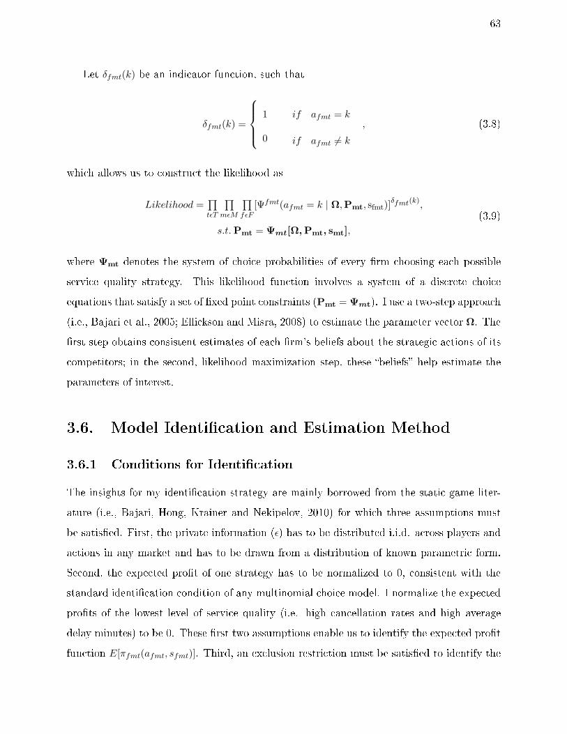
63
Let δfmt(k) be an indicator function, such that
δfmt(k) =
1
0
if afmt = k
if afmt = k
, (3.8)
which allows us to construct the likelihood as
Likelihood =∏tϵT
∏mϵM
∏fϵF
[Ψfmt(afmt = k | Ω,Pmt, sfmt)]δfmt(k),
s.t.Pmt = Ψmt[Ω,Pmt, smt],
(3.9)
where Ψmt denotes the system of choice probabilities of every rm choosing each possible
service quality strategy. This likelihood function involves a system of a discrete choice
equations that satisfy a set of xed point constraints (Pmt = Ψmt). I use a two-step approach
(i.e., Bajari et al., 2005; Ellickson and Misra, 2008) to estimate the parameter vector Ω. The
rst step obtains consistent estimates of each rm's beliefs about the strategic actions of its
competitors; in the second, likelihood maximization step, these beliefs help estimate the
parameters of interest.
3.6. Model Identication and Estimation Method
3.6.1 Conditions for Identication
The insights for my identication strategy are mainly borrowed from the static game liter-
ature (i.e., Bajari, Hong, Krainer and Nekipelov, 2010) for which three assumptions must
be satised. First, the private information (ϵ) has to be distributed i.i.d. across players and
actions in any market and has to be drawn from a distribution of known parametric form.
Second, the expected prot of one strategy has to be normalized to 0, consistent with the
standard identication condition of any multinomial choice model. I normalize the expected
prots of the lowest level of service quality (i.e. high cancellation rates and high average
delay minutes) to be 0. These rst two assumptions enable us to identify the expected prot
function E[πfmt(afmt, sfmt)]. Third, an exclusion restriction must be satised to identify the

64
deterministic part of the prot function (i.e., Πfmt(sfmt, afmt, a−fmt)), given choice probabil-
ities and expected prots E[πfmt(afmt, sfmt)]. The relation between Πfmt(sfmt, afmt, a−fmt)
and E[πfmt(afmt, sfmt)] can be written as
E[πfmt(afmt, sfmt)] =∑
a−fmt
Πfmt(sfmt, afmt, a−fmt)P−fmt, (3.10)
where P−fmt = Πjmt =fmt Prjmt(ajmt | sjmt).
The identication of Πfmt(sfmt, afmt, a−fmt) then is equivalent to a problem of nding a
solution to the system of equations in Equation 3.10. The choice probability of each rm
is a function of its beliefs regarding the conditional probabilities of its rivals, as well as
state variables. If rms share exactly the same value for each state variable, this system of
equations, which is not full rank, cannot be solved, because the number of unknowns are
more than the number of informative equations. To solve this system of equations, I must
ensure that there are one or more covariates that enter the payo function of rm f in market
m at tine t but do not enter the payo functions of other rms in the same market at the
same time, or the payo functions of rm f in other markets/at other time. Among the state
variables we have, departures performed and capacity utilization vary across rms, markets
and time. That is to say, values of these state variables are dierent across rms in the same
market at the same time, and for each rm, values of these state variables are dierent across
markets and time as well. Moreover, I include rm, market, year, and quarter xed-eect
terms in the payo functions, which further guarantee the uniqueness of each equation in the
system. This system of equations is a full rank matrix, thus the coecient of a state variable
can be identied by the variation of the focal variable and the corresponding variation of
the service quality choice in the data. Specically, the coecients of departures performed
and capacity utilization can be identied by the variation of service quality choice at the
rm-market-time level in response to variations of these state variables at the rm-market-
time level. The coecients of hub of origin and hub of destination can be identied by the
service quality choice variation at the same time in dierent rm-market units, in response
to variations of these state variables at across rm and market. The coecients of the state
variables which vary at the market level (i.e., number of business, income per capita, and

65
competitor's hub), can be identied by the service quality choice variation of the same rm
in dierent market-time units, in response to the variation of these state variables across
markets and time.
3.6.2 Existence and Multiplicity of Equilibria
The existence of equilibria is ensured if the system of equations given by Equation 3.6
has at least one solution. The choice probabilities Ψ are monotonic, continuous, and strictly
bounded within the set (0, 1), given the Type I Extreme Value distribution assumption about
ϵ. The existence of solutions to the system of equation then follows, according to Brower's
Fixed Point Theorem (McKelvey and Palfrey, 1995).
It is possible that multiple equilibria exist (i.e., multiple solutions to the system of equa-
tions given by Equation 3.6). To remedy this potential challenge I: (1) include rm xed
eects to make the game asymmetric (i.e., the set of prots earned when United chooses
high service quality while Southwest chooses low service quality is dierent from the set of
prots earned when United chooses low service quality while Southwest chooses high service
quality), such that I can recover at least the estimates of a dominant equilibrium (i.e., an
equilibrium most likely to happen); (2) impose a standard assumption in two-step methods
for estimating incomplete information games, which states that given a set of value of Ω
and X, players (or nature) select only one equilibrium from all possible equilibria; and (3)
assume that rms do not switch to other equilibria as long as Ω and X do not change (i.e.,
Vitorino 2012).
3.6.3 Endogeneity
Table 3.2 presents a list of the variables used to dene the state of each rm. For market
characteristics, we use measurements of the size and value of the market, such as the number
of businesses and income per capita. Additionally, I also include a dummy variable that tracks
if the market is a hub for a competitor. For rm characteristics, I use measurements that
correlate with costs and/or revenues, such as the volume of ight departures performed and
capacity utilitization. Finally, it is likely that the decisions regarding service quality might
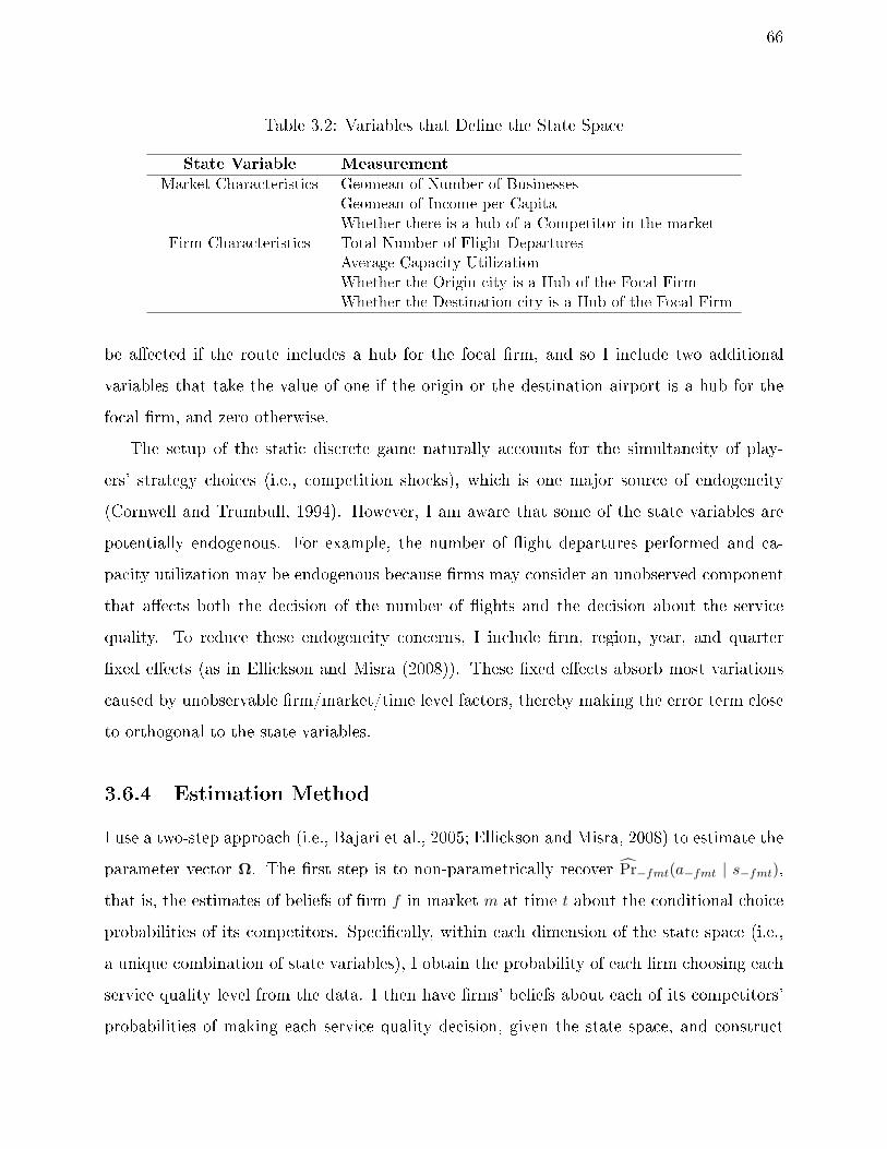
66
Table 3.2: Variables that Dene the State Space
State Variable Measurement
Market Characteristics Geomean of Number of BusinessesGeomean of Income per CapitaWhether there is a hub of a Competitor in the market
Firm Characteristics Total Number of Flight DeparturesAverage Capacity UtilizationWhether the Origin city is a Hub of the Focal FirmWhether the Destination city is a Hub of the Focal Firm
be aected if the route includes a hub for the focal rm, and so I include two additional
variables that take the value of one if the origin or the destination airport is a hub for the
focal rm, and zero otherwise.
The setup of the static discrete game naturally accounts for the simultaneity of play-
ers' strategy choices (i.e., competition shocks), which is one major source of endogeneity
(Cornwell and Trumbull, 1994). However, I am aware that some of the state variables are
potentially endogenous. For example, the number of ight departures performed and ca-
pacity utilization may be endogenous because rms may consider an unobserved component
that aects both the decision of the number of ights and the decision about the service
quality. To reduce these endogeneity concerns, I include rm, region, year, and quarter
xed eects (as in Ellickson and Misra (2008)). These xed eects absorb most variations
caused by unobservable rm/market/time level factors, thereby making the error term close
to orthogonal to the state variables.
3.6.4 Estimation Method
I use a two-step approach (i.e., Bajari et al., 2005; Ellickson and Misra, 2008) to estimate the
parameter vector Ω. The rst step is to non-parametrically recover Pr−fmt(a−fmt | s−fmt),
that is, the estimates of beliefs of rm f in market m at time t about the conditional choice
probabilities of its competitors. Specically, within each dimension of the state space (i.e.,
a unique combination of state variables), I obtain the probability of each rm choosing each
service quality level from the data. I then have rms' beliefs about each of its competitors'
probabilities of making each service quality decision, given the state space, and construct

67
the beliefs of competitors' aggregated service quality decision probabilities ρr−fmt, where
r = 1, ...,K, for each rm f in each market m at each time t. Knowing ρr−fmt, we proceed
the second step, which is to choose the parameters that maximize the following likelihood
function
L(Ω) =∏tϵT
∏mϵM
∏fϵF
[Ψfmt(afmt = k | Pmt, sfmt)]δfmt(k), (3.11)
where Pmt denotes the set of estimated choice probabilities (i.e., belief) of all rms in market
m at time t (including the probabilities of every rm in the focal market taking every pos-
sible service quality action). I use the in-sample predictions from the maximum likelihood
estimation to update rms' beliefs on competitors' service quality probabilities, and then
perform the maximum likelihood estimation with the updated beliefs. I proceed with these
two steps iteratively until I achieve consistent estimates of Ω3.
3.7. Results
In the model section, I conceptualize rms' service quality choices as K discrete levels. In
practice, I implement the service quality choices to be four levels: high cancellation and high
delay, high cancellation and low delay, low cancellation and high delay, low cancellation and
low delay. I present results of robustness checks to show that the four-level discretization
does not change the results qualitatively.
3.7.1 Analysis of Parameter Estimates
I present the estimation results in Table 3.3.4 In terms of market characteristics, I nd
that the number of businesses increases the likelihood that rms adopt a high quality level,
with a low cancellation, low delay service (the expected multinomial log-odds for the low
cancellation low delay service, relative to the high cancellation high delay service increase by
3Consistent estimates are dened as converged estimates between the last two rounds of iteration. Theconvergence criterior is | Ωt+1 − Ωt |< 1.0E−8.
4The prots of the high cancellation, high delay service quality decision are normalized to 0 for identi-cation.
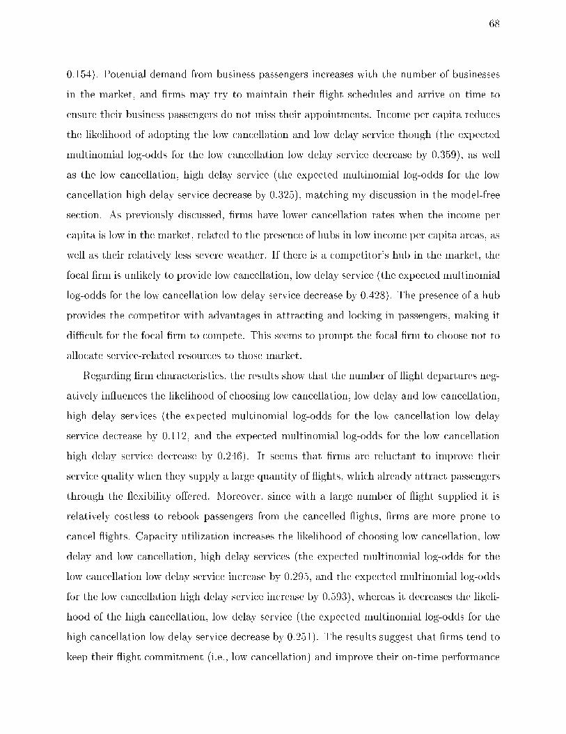
68
0.154). Potential demand from business passengers increases with the number of businesses
in the market, and rms may try to maintain their ight schedules and arrive on time to
ensure their business passengers do not miss their appointments. Income per capita reduces
the likelihood of adopting the low cancellation and low delay service though (the expected
multinomial log-odds for the low cancellation low delay service decrease by 0.359), as well
as the low cancellation, high delay service (the expected multinomial log-odds for the low
cancellation high delay service decrease by 0.325), matching my discussion in the model-free
section. As previously discussed, rms have lower cancellation rates when the income per
capita is low in the market, related to the presence of hubs in low income per capita areas, as
well as their relatively less severe weather. If there is a competitor's hub in the market, the
focal rm is unlikely to provide low cancellation, low delay service (the expected multinomial
log-odds for the low cancellation low delay service decrease by 0.428). The presence of a hub
provides the competitor with advantages in attracting and locking in passengers, making it
dicult for the focal rm to compete. This seems to prompt the focal rm to choose not to
allocate service-related resources to those market.
Regarding rm characteristics, the results show that the number of ight departures neg-
atively inuences the likelihood of choosing low cancellation, low delay and low cancellation,
high delay services (the expected multinomial log-odds for the low cancellation low delay
service decrease by 0.112, and the expected multinomial log-odds for the low cancellation
high delay service decrease by 0.246). It seems that rms are reluctant to improve their
service quality when they supply a large quantity of ights, which already attract passengers
through the exibility oered. Moreover, since with a large number of ight supplied it is
relatively costless to rebook passengers from the cancelled ights, rms are more prone to
cancel ights. Capacity utilization increases the likelihood of choosing low cancellation, low
delay and low cancellation, high delay services (the expected multinomial log-odds for the
low cancellation low delay service increase by 0.295, and the expected multinomial log-odds
for the low cancellation high delay service increase by 0.593), whereas it decreases the likeli-
hood of the high cancellation, low delay service (the expected multinomial log-odds for the
high cancellation low delay service decrease by 0.251). The results suggest that rms tend to
keep their ight commitment (i.e., low cancellation) and improve their on-time performance

69
(i.e., low delay) when they are able to manage their capacity well. If they cannot do well by
decreasing both cancellation and delay, at least they try to keep their service commitment
(i.e., low cancellation), in order to not impact a large number of passengers in a fully or close
to fully booked ight. Finally, the results related to the existence of hub eects suggest that
it is costly for rms to provide high service quality in their hubs (when departing from a
hub, the expected multinomial log-odds for the low cancellation low delay service decrease
by 0.637, the expected multinomial log-odds for the low cancellation high delay decrease
by 0.189, and the expected multinomial log-odds for the high cancellation low delay service
decrease by 0.278; when ying to a hub, the expected multinomial log-odds for the low can-
cellation high delay service decrease by 0.463, and the expected multinomial log-odds for
the low cancellation high delay service decrease by 0.566), probably because they have busy
and complex patterns of scheduling with ights coming from and going to places in their
networks, leading to shortages of resources (i.e., airport gates, runway slots).
I complete my discussion of the results by discussing the eect of competitors' choices
on the decision of the service quality level. Here, the main nding is that I nd evidence of
dierentiation strategies by the rms. When rms believe that competitor are more likely to
provide a high service quality of low cancellation, low delay services, the focal rm is likely to
provide the opposite low level of service quality with high cancellations and high delays (the
expected multinomial log-odds for the low cancellation low delay service, relative to the high
cancellation high delay service, decrease by 1.022, the expected multinomial log-odds for the
low cancellation high delay service decrease by 1.914, and the expected multinomial log-odds
for the high cancellation low delay service decrease by 1.255). Instead of being motivated,
rms seem reluctant to improve their service quality to match their competitor who already
maintain their service commitment and provide good on-time performance, probably because
the focal rm would have to allocate signicant resources to reach this level of service quality.
Additionally, rms are likely to provide high service quality (low cancellation, low delay)
when they believe their competitors are likely to perform poorly in one of the dimensions.
That is, one unit increase in competitors' probability of providing high cancellation low delay
services (low cancellation high delay service) increases the expected multinomial log-odds for
low cancellation low delay service (of focal rm) by 0.921 (2.2). In other words, rms are

70
motivated to provide good services in both dimensions when competitors provide good service
in one dimension but poor service in the other, as a way to dierentiate themselves from the
competition. Finally, the focal rm probably adopts a high cancellation, low delay service
if it believes its competitors are going to oer high delay, low cancellation and/or low delay,
and high cancellation services. Specically, one unit increase in competitors' probability of
providing high cancellation low delay services (low cancellation high delay service) increases
the expected multinomial log-odds for low cancellation low delay service (of focal rm) by
0.99 (2.395). However, the likelihood of providing high delay, low cancellation service is not
aected by rms' beliefs about their competitors' service quality decisions. These results
suggest that rms are likely to work on their on-time performance but not change how
well they keep their ight commitments in a market when they are threatened by their
competitors' service performance.
3.7.2 Discussion of Drivers of Service Quality Decisions
In section 3.7.1, I discussed the eects of market characteristics, rm characteristics, and
competition on the joint decision of ight cancellations and delays. However, it is not clear
whether rms follow dierent decision processes to determine the level of ight cancellation
and the level of ight delay. To provide in-depth insights on service quality decisions, I
discuss drivers of ight cancellation and drivers of ight delay individually, and seek to nd
dierences in the decision processes for these two service dimensions.
I list the state variables that signicantly inuence the ight cancellation decision in Table
3.4. In our data, most markets with low income per capita are important air transportation
centers (e.g., Atlanta, Dallas, Miami) or are located in the south, whereas many markets
with high income per capita are not air transportation centers and/or are located in the
north (e.g., Boston, Baltimore, Minneapolis). The results suggest that rms tend to not
cancel many ights in air transportation centers located in the south, the result is consistent
with the intuitions that rms cancel more ights in markets that are not important and that
the weather conditions drive ight cancellations.
Firms are also likely to cancel more ights (1) as their supply of ights increases and
(2) when they have a hub airport in the market. They are not likely to cancel ights as

71
Table 3.3: Parameter Estimates
X Variable Low Can-
cel + Low
Delay
Low Can-
cel + High
Delay
High
Cancel +
Low Delay
Intercept 1.324***(0.199)
1.465***(0.206)
-0.437*(3.33)
Number of Businesses 0.154**(0.076)
-0.005(0.080)
0.038(0.081)
Income per Capita -0.359***(0.098)
-0.325**(0.105)
-0.039(0.103)
Competitors' Hub -0.428***(0.156)
-0.072(0.177)
0.132(0.172)
Total Number of Flight Departures -0.112*(0.066)
-0.246***(0.069)
-0.060(0.069)
Capacity Utilization 0.295***(0.062)
0.593***(0.067)
-0.251***(0.064)
Hub Origin -0.637***(0.090)
-0.189**(0.096)
-0.278***(0.094)
Hub Destination -0.463***(0.090)
-0.566***(0.096)
0.146(0.094)
Belief of Competitors' H-H Probability 0.019(0.418)
-0.179(0.437)
-0.147(0.432)
Belief of Competitors' H-L Probability 0.921*(0.475)
0.823(0.517)
0.990**(0.471)
Belief of Competitors' L-H Probability 2.200***(0.518)
0.837(0.557)
2.395***(0.548)
Belief of Competitors' L-L Probability -1.022**(0.471)
-1.914***(0.518)
-1.255**(0.506)
Notes: H and L refer to high and low, presented as cancellation and delay, in that order.Standard errors are in parenthesis.* p < 0.10. ** p < 0.05. *** p < 0.01.
their aircraft capacity utilization increases. We can infer from these results that the ight
cancellation decision relates closely to capacity management and scheduling exibility. Firms
are unlikely to cancel ights when it is protable to let their aircrafts take o (i.e., most of
seats are sold). When rms have large ight supply in a market, they have the exibility to
reschedule passengers to the next ights. Similarly, when rms have a hub in the market,
they can more exibly reschedule passengers when they cancel some ights. The convenience
of rescheduling makes rms more likely to cancel some ights.
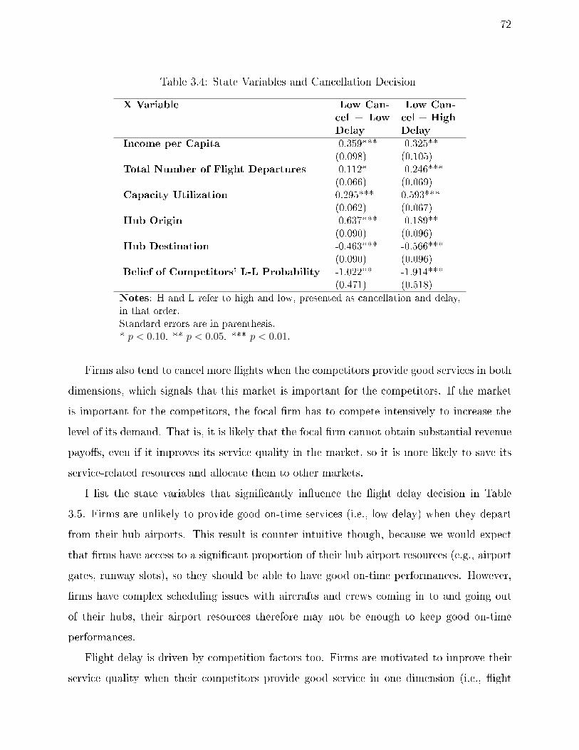
72
Table 3.4: State Variables and Cancellation Decision
X Variable Low Can-
cel + Low
Delay
Low Can-
cel + High
Delay
Income per Capita -0.359***(0.098)
-0.325**(0.105)
Total Number of Flight Departures -0.112*(0.066)
-0.246***(0.069)
Capacity Utilization 0.295***(0.062)
0.593***(0.067)
Hub Origin -0.637***(0.090)
-0.189**(0.096)
Hub Destination -0.463***(0.090)
-0.566***(0.096)
Belief of Competitors' L-L Probability -1.022**(0.471)
-1.914***(0.518)
Notes: H and L refer to high and low, presented as cancellation and delay,in that order.Standard errors are in parenthesis.* p < 0.10. ** p < 0.05. *** p < 0.01.
Firms also tend to cancel more ights when the competitors provide good services in both
dimensions, which signals that this market is important for the competitors. If the market
is important for the competitors, the focal rm has to compete intensively to increase the
level of its demand. That is, it is likely that the focal rm cannot obtain substantial revenue
payos, even if it improves its service quality in the market, so it is more likely to save its
service-related resources and allocate them to other markets.
I list the state variables that signicantly inuence the ight delay decision in Table
3.5. Firms are unlikely to provide good on-time services (i.e., low delay) when they depart
from their hub airports. This result is counter intuitive though, because we would expect
that rms have access to a signicant proportion of their hub airport resources (e.g., airport
gates, runway slots), so they should be able to have good on-time performances. However,
rms have complex scheduling issues with aircrafts and crews coming in to and going out
of their hubs, their airport resources therefore may not be enough to keep good on-time
performances.
Flight delay is driven by competition factors too. Firms are motivated to improve their
service quality when their competitors provide good service in one dimension (i.e., ight

73
cancellation or ight delay). When they respond to competitors' service decisions, they tend
to work on their delays. Firms' on-time performance in a market depends largely on their
operational schedules, such as the relevant aircraft and crew schedules, time block, and so
on. These operational schedules are exible to adjust, compared with the importance or
protability of the market. Firms therefore respond more readily to competitors' service
quality decisions by adjusting their on-time performances. In contrast, rms are unlikely to
reduce their ight delays when competitors provide good services in both dimensions. They
simply are unlikely to gain any revenue payos by improving service quality if the market is
important to the competitor, thus they choose to allocate their resources to other markets.
To summarize, the results suggest that ight cancellation and ight delay decisions are
driven by dierent set of factors. Specically, ight cancellation decisions are inuenced
mainly by cost-benet concerns, such as the ease of rescheduling after ight cancellation,
the amount of penalty costs (e.g., voucher for food and hotel, brand image damage) from
ight cancellation, and the extent of costs saved from cancelling empty ights. These cost-
benet concerns are inuenced by the number of ight departures, capacity utilization, and
the presence of hub airports in the market. Firms respond to competition by adjusting
their ight delay levels such that they are able to dierentiate their services from those of
competitors. In addition, ight delay decisions are driven by the presence of hub in the
origin airport, due to the complicated aircraft and crew scheduling issues in hub airports.
3.7.3 Robustness Checks
To make sure that the results presented in the previous section are not driven by the four-
level service quality discretization, I run two sets of robustness checks. In the rst robustness
check (section 3.7.3.1), I trichotomize the cancellation and delay data (i.e., high, medium,
low levels of cancellation and delay) in each market, and estimate the model again using the
estimation method proposed in 3.6.4. The data trichotomization enables us to distinguish
the good (i.e., low cancellation; low delay) and bad (i.e., high cancellation; high delay)
services from those uctuating in the middle (i.e., medium cancellation; medium delay), and
therefore may generate new insights. In the second robustness check (section 3.7.3.2), I run a
reduced-form analysis, keeping the original continuous (median-centered) values of the delay
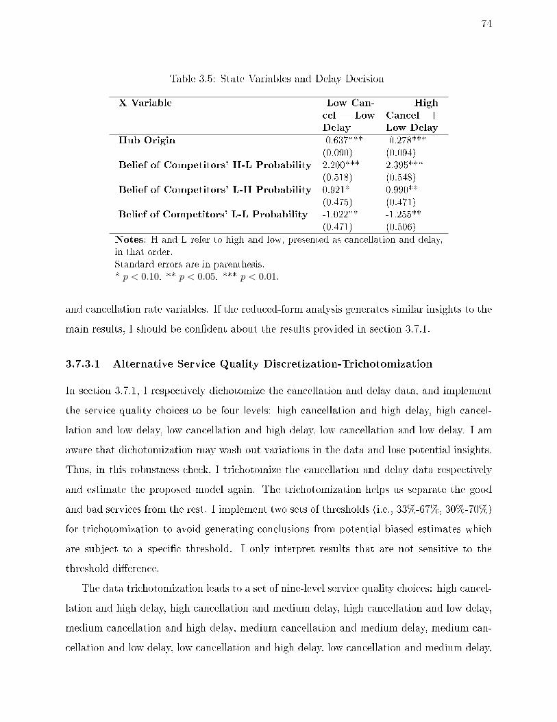
74
Table 3.5: State Variables and Delay Decision
X Variable Low Can-
cel + Low
Delay
High
Cancel +
Low Delay
Hub Origin -0.637***(0.090)
-0.278***(0.094)
Belief of Competitors' H-L Probability 2.200***(0.518)
2.395***(0.548)
Belief of Competitors' L-H Probability 0.921*(0.475)
0.990**(0.471)
Belief of Competitors' L-L Probability -1.022**(0.471)
-1.255**(0.506)
Notes: H and L refer to high and low, presented as cancellation and delay,in that order.Standard errors are in parenthesis.* p < 0.10. ** p < 0.05. *** p < 0.01.
and cancellation rate variables. If the reduced-form analysis generates similar insights to the
main results, I should be condent about the results provided in section 3.7.1.
3.7.3.1 Alternative Service Quality Discretization-Trichotomization
In section 3.7.1, I respectively dichotomize the cancellation and delay data, and implement
the service quality choices to be four levels: high cancellation and high delay, high cancel-
lation and low delay, low cancellation and high delay, low cancellation and low delay. I am
aware that dichotomization may wash out variations in the data and lose potential insights.
Thus, in this robustness check, I trichotomize the cancellation and delay data respectively
and estimate the proposed model again. The trichotomization helps us separate the good
and bad services from the rest. I implement two sets of thresholds (i.e., 33%-67%, 30%-70%)
for trichotomization to avoid generating conclusions from potential biased estimates which
are subject to a specic threshold. I only interpret results that are not sensitive to the
threshold dierence.
The data trichotomization leads to a set of nine-level service quality choices: high cancel-
lation and high delay, high cancellation and medium delay, high cancellation and low delay,
medium cancellation and high delay, medium cancellation and medium delay, medium can-
cellation and low delay, low cancellation and high delay, low cancellation and medium delay,
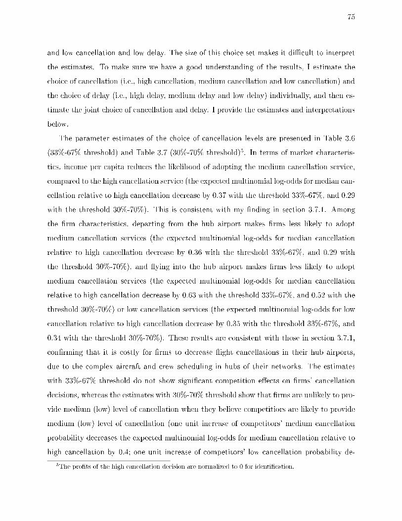
75
and low cancellation and low delay. The size of this choice set makes it dicult to interpret
the estimates. To make sure we have a good understanding of the results, I estimate the
choice of cancellation (i.e., high cancellation, medium cancellation and low cancellation) and
the choice of delay (i.e., high delay, medium delay and low delay) individually, and then es-
timate the joint choice of cancellation and delay. I provide the estimates and interpretations
below.
The parameter estimates of the choice of cancellation levels are presented in Table 3.6
(33%-67% threshold) and Table 3.7 (30%-70% threshold)5. In terms of market characteris-
tics, income per capita reduces the likelihood of adopting the medium cancellation service,
compared to the high cancellation service (the expected multinomial log-odds for median can-
cellation relative to high cancellation decrease by 0.37 with the threshold 33%-67%, and 0.29
with the threshold 30%-70%). This is consistent with my nding in section 3.7.1. Among
the rm characteristics, departing from the hub airport makes rms less likely to adopt
medium cancellation services (the expected multinomial log-odds for median cancellation
relative to high cancellation decrease by 0.36 with the threshold 33%-67%, and 0.29 with
the threshold 30%-70%), and ying into the hub airport makes rms less likely to adopt
medium cancellation services (the expected multinomial log-odds for median cancellation
relative to high cancellation decrease by 0.63 with the threshold 33%-67%, and 0.52 with the
threshold 30%-70%) or low cancellation services (the expected multinomial log-odds for low
cancellation relative to high cancellation decrease by 0.35 with the threshold 33%-67%, and
0.34 with the threshold 30%-70%). These results are consistent with those in section 3.7.1,
conrming that it is costly for rms to decrease ight cancellations in their hub airports,
due to the complex aircraft and crew scheduling in hubs of their networks. The estimates
with 33%-67% threshold do not show signicant competition eects on rms' cancellation
decisions, whereas the estimates with 30%-70% threshold show that rms are unlikely to pro-
vide medium (low) level of cancellation when they believe competitiors are likely to provide
medium (low) level of cancellation (one unit increase of competitors' medium cancellation
probability decreases the expected multinomial log-odds for medium cancellation relative to
high cancellation by 0.4; one unit increase of competitors' low cancellation probability de-
5The prots of the high cancellation decision are normalized to 0 for identication.
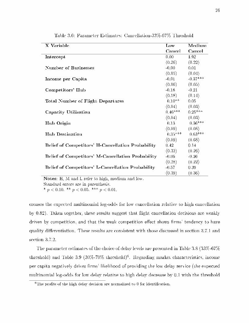
76
Table 3.6: Parameter Estimates: Cancellation-33%-67% Threshold
X Variable Low
Cancel
Medium
Cancel
Intercept 0.00(0.26)
1.92(0.22)
Number of Businesses -0.00(0.05)
0.01(0.04)
Income per Capita -0.01(0.06)
-0.37***(0.05)
Competitors' Hub -0.18(0.18)
-0.21(0.14)
Total Number of Flight Departures -0.10**(0.04)
0.05(0.03)
Capacity Utilization 0.46***(0.04)
0.25***(0.03)
Hub Origin -0.13(0.09)
-0.36***(0.08)
Hub Destination -0.35***(0.09)
-0.63***(0.68)
Belief of Competitors' H-Cancellation Probability 0.42(0.32)
0.14(0.26)
Belief of Competitors' M-Cancellation Probability -0.06(0.28)
-0.36(0.22)
Belief of Competitors' L-Cancellation Probability -0.57(0.39)
0.39(0.36)
Notes: H, M and L refer to high, medium and low.Standard errors are in parenthesis.* p < 0.10. ** p < 0.05. *** p < 0.01.
creases the expected multinomial log-odds for low cancellation relative to high cancellation
by 0.82). Taken together, these results suggest that ight cancellation decisions are weakly
driven by competition, and that the weak competition eect shows rms' tendency to have
quality dierentiation. These results are consistent with those discussed in section 3.7.1 and
section 3.7.2.
The parameter estimates of the choice of delay levels are presented in Table 3.8 (33%-67%
threshold) and Table 3.9 (30%-70% threshold)6. Regarding market characteristics, income
per capita negatively drives rms' likelihood of providing the low delay service (the expected
multinomial log-odds for low delay relative to high delay decrease by 0.1 with the threshold
6The prots of the high delay decision are normalized to 0 for identication.

77
Table 3.7: Parameter Estimates: Cancellation-30%-70% Threshold
X Variable Low
Cancel
Medium
Cancel
Intercept -0.46(0.30)
1.95***(0.24)
Number of Businesses 0.10(0.06)
0.03(0.05)
Income per Capita 0.08(0.06)
-0.29***(0.05)
Competitors' Hub -0.24(0.18)
-0.11(0.14)
Total Number of Flight Departures -0.07(0.05)
0.07**(0.04)
Capacity Utilization 0.51***(0.04)
0.30***(0.03)
Hub Origin -0.15(0.10)
-0.29***(0.07)
Hub Destination -0.34***(0.10)
-0.52***(0.07)
Belief of Competitors' H-Cancellation Probability 0.49(0.36)
0.21(0.28)
Belief of Competitors' M-Cancellation Probability 0.18(0.27)
-0.40**(0.20)
Belief of Competitors' L-Cancellation Probability -0.82*(0.43)
0.41(0.38)
Notes: H, M and L refer to high, medium and low.Standard errors are in parenthesis.* p < 0.10. ** p < 0.05. *** p < 0.01.
33%-67%, and 0.12 with the threshold 30%-70%), and the presence of a competitor's hub
airport negatively drive rms' likelihood of providing the low delay service (the expected
multinomial log-odds for low delay relative to high delay decrease by 0.31 with the threshold
33%-67%, and 0.35 with the threshold 30%-70%). These eects are consistent with those
provided in section 3.7.1. Table 3.8 and Table 3.9 show three eects of rm characteristics
on ight delay levels that are not clear in section 3.7.1: the number of ight departures
positively inuences the choice of the medium delay service (the expected multinomial log-
odds for medium delay relative to high delay increase by 0.11 with the threshold 33%-67%,
and 0.16 with the threshold 30%-70%); capacity utilization negatively drive the likelihood
of providing the low delay service (the expected multinomial log-odds for low delay relative
78
to high delay decrease by 0.19 with both thresholds) and the medium delay service (the
expected multinomial log-odds for low delay relative to high delay decrease by 0.06 with the
threshold 33%-67%, and 0.07 with the threshold 30%-70%); and rms tend to provide low
delay service (the expected multinomial log-odds for low delay relative to high delay increase
by 0.15 with the threshold 33%-67%) or medium delay service (the expected multinomial
log-odds for medium delay relative to high delay increase by 0.17 with the threshold 33%-
67%) when ying to their hub airports. When a rm has many ight departures in a market,
it is likely to avoid long ight delays because the long-time delay of one ight may cause
delays of other ights, given the limited gate slots; however, at the same time, it is hard to
keep all ights on time because of the complicated aircraft and crew scheduling issues with
so many ight departures. As a result, rms are likely to provide medium level of delay as
the number of ight departures increases. It is hard to manage boarding and keep ights
on-time as the planes get fuller, thus rms are not likely to provide low delay (or sometimes
medium delay) services as capacity utilization increases. When aircrafts are ew into the
hub airports, it is likely that some other scheduled ights are awaiting for these aircrafts,
thus rms have incentives to decrease delays to avoid carry over delays for other ights.
When departing from the origin airport, rms are not likely to provide the low delay service
(the expected multinomial log-odds for low delay relative to high delay decrease by 0.43 with
the threshold 33%-67%, and 0.51 with the threshold 30%-70%), which is consistent with the
results provided in section 3.7.1. In terms of competition eects, Table 3.8 and 3.9 both show
that rms are likely to provide the medium delay service (the expected multinomial log-odds
for medium delay relative to high delay increase by 1 with the threshold 33%-67%, and 0.75
with the threshold 30%-70%) and/or the low delay service (the expected multinomial log-
odds for low delay relative to high delay increase by 0.66 with the threshold 33%-67%, and
0.71 with the threshold 30%-70%) when competitors provides high delay services, and that
rms are likely to provide the low delay service when competitors provides medium delay
services (the expected multinomial log-odds for low delay relative to high delay increase by
1.92 with the threshold 33%-67%, and 1.71 with the threshold 30%-70%). These results
suggest that rms try to dierentiate their services from competitors', which is consistent
with the insights provided in section 3.7.1 and 3.7.2. Comparing the competition eects in

79
Table 3.8: Parameter Estimates: Delay-33%-67% Threshold
X Variable Low
Delay
Medium
Delay
Intercept 0.24(0.21)
-0.39*(0.21)
Number of Businesses -0.03(0.05)
-0.05(0.05)
Income per Capita -0.10**(0.05)
0.03(0.05)
Competitors' Hub -0.31**(0.14)
-0.20(0.14)
Total Number of Flight Departures 0.01(0.04)
0.11***(0.04)
Capacity Utilization -0.19***(0.03)
-0.06*(0.03)
Hub Origin -0.43***(0.08)
-0.10(0.08)
Hub Destination 0.15*(0.08)
0.17**(0.08)
Belief of Competitors' H-Delay Probability 0.66*(0.36)
1.00***(0.35)
Belief of Competitors' M-Delay Probability 1.92***(0.59)
0.08(0.59)
Belief of Competitors' L-Delay Probability -0.17(0.32)
0.48(0.33)
Notes: H, M and L refer to high, medium and low.Standard errors are in parenthesis.* p < 0.10. ** p < 0.05. *** p < 0.01.
Table 3.8 and 3.9 with those in Table 3.6 and 3.7, we may see that rms are more eager
to provide better services than competitors in the delay dimension than the cancellation
dimension. This is consistent with the ndings in section 3.7.1 that when rms react to
service competition, they are likely to decrease ight delay rather than cancellation.
After analyzing how cancellation and delay decisions are driven by market characteristics,
rm characteristics and competition respectively, we provide parameter estimates of the joint
choice of cancellation and delay services in Table 3.10 to Table 3.11 (33%-67% threshold) and
Table 3.12 to Table 3.13 (30%-70% threshold)7. Regarding market characteristics, Table 3.12
shows that number of business in the market has a marginally signicant positive eect on the
7The prots of the high cancellation and high delay service are normalized to 0 for identication.
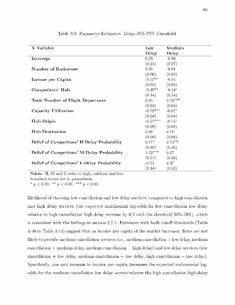
80
Table 3.9: Parameter Estimates: Delay-30%-70% Threshold
X Variable Low
Delay
Medium
Delay
Intercept 0.29(0.24)
-0.09(0.22)
Number of Businesses 0.00(0.06)
-0.04(0.05)
Income per Capita -0.12**(0.05)
-0.05(0.05)
Competitors' Hub -0.35**(0.14)
-0.24*(0.14)
Total Number of Flight Departures 0.05(0.04)
0.16***(0.04)
Capacity Utilization -0.19***(0.04)
-0.07*(0.04)
Hub Origin -0.51***(0.09)
-0.15*(0.08)
Hub Destination 0.08(0.08)
0.11(0.08)
Belief of Competitors' H-Delay Probability 0.71*(0.40)
0.75**(0.36)
Belief of Competitors' M-Delay Probability 1.70***(0.51)
0.27(0.49)
Belief of Competitors' L-Delay Probability -0.23(0.34)
0.37(0.33)
Notes: H, M and L refer to high, medium and low.Standard errors are in parenthesis.* p < 0.10. ** p < 0.05. *** p < 0.01.
likelihood of choosing low cancellation and low delay services, compared to high cancellation
and high delay services (the expected multinomial log-odds for low cancellation low delay
relative to high cancellation high delay increase by 0.2 with the threshold 30%-70%), which
is consistent with the ndings in section 3.7.1. Estimates with both cuto thresholds (Table
3.10 to Table 3.13) suggest that as income per capita of the market increases, rms are not
likely to provide medium cancellation services (i.e., medium cancellation + low delay, medium
cancellation + medium delay, medium cancellation + high delay) and low delay services (low
cancellation + low delay, medium cancellation + low delay, high cancellation + low delay).
Specically, one unit increase in income per capita decreases the expected multinomial log-
odds for the medium cancellation low delay service relative the high cancellation high delay

81
service by 0.43 with the threshold 33%-67%, and 0.39 with the threshold 30%-70%; one unit
increase in income per capita decreases the expected multinomial log-odds for the medium
cancellation medium delay service by 0.44 with both thresholds; one unit increase in income
per capita decreases the expected multinomial log-odds for the medium cancellation high
delay service by 0.42 with the threshold 33%-67%, and 0.36 with the threshold 30%-70%;
one unit increase in income per capita decreases the expected multinomial log-odds for the
low cancellation low delay service relative the high cancellation high delay service by 0.21
with the threshold 33%-67%, and 0.20 with the threshold 30%-70%; one unit increase in
income per capita decreases the expected multinomial log-odds for the high cancellation low
delay service by 0.25 with the threshold 33%-67%, and 0.29 with the threshold 30%-70%.
These eects are consistent with those in Table 3.6 to Table 3.9, as well as those provided
in section 3.7.1. Both Table 3.10 and Table 3.12 suggest that if there is a competitor's hub
present in the market, rms are unlikely to provide the medium cancellation and low delay
service, compared to the high cancellation and high delay service (the expected multinomial
log-odds for the medium cancellation low delay service relative the high cancellation high
delay service decrease by 0.57 with the threshold 33%-67%, and 0.42 with the threshold
30%-70%). As discussed in section 3.7.1, the presence of a hub airport grants the competitor
advantages in attracting and locking in passengers, making it dicult for the focal rm
to compete. This seems to prompt the focal rm to choose not to allocate service-related
resources to those markets.
In terms of rm characteristics, Table 3.10 to Table 3.13 show that as the number of ight
departures increases, rms are more likely to provide medium/high cancellation and medium
delay services. Specically, one unit increase in the number of ight departures increases the
expected multinomial log-odds for the medium cancellation medium delay service (relative to
the high cancellation high delay service) by 0.11 with the threshold 33%-67%, and 0.20 with
the threshold 30%-70%; and one unit increase in the number of ight departures increases
the expected multinomial log-odds for the high cancellation medium delay service by 0.12
with the threshold 33%-67%, and 0.19 with the threshold 30%-70%. These eects reect
the results in Table 3.8 and 3.9. That is, rms are likely to provide medium delay services
when they have a large number of ights serving the market. Moreover, these eects also
82
suggest that rms are not likely to provide low cancellation services (compared to the high
cancellation high delay service) given a large number of ight departures, which is consistent
with ndings in section 3.7.1. With the threshold 33%-67% (30%-70%), one unit increase
in capacity utilization increases the expected multinomial log-odds for the low cancellation
low delay service (relative to the high cancellation high delay service) by 0.28 (0.33); it
increases the expected multinomial log-odds for the low cancellation medium delay service
by 0.48 (0.55); it increases the expected multinomial log-odds for the low cancellation high
delay service by 0.46 (0.49); it increases the expected multinomial log-odds for the medium
cancellation medium delay service by 0.19 (0.26); it increases the expected multinomial log-
odds for the medium cancellation high delay service by 0.28 (0.34); and it decreases the
expected multinomial log-odds for the high cancellation low delay service by 0.21 (0.18). To
summarize, as capacity utilization increases, rms are more likely to provide low/medium
cancellation services, because of the increased cancellation costs as planes get full, which is
consistent with ndings in section 3.7.1. Consistent with results provided in Table 3.6-3.9,
Table 3.10 to Table 3.13 show that when departing from hub airports, rms are not likely to
provide medium cancellation services and/or low delay services (the expected multinomial
log-odds for the medium cancellation low delay service decreases by 0.92 with the threshold
33%-67%, and 0.83 with the threshold 30%-70%; the expected multinomial log-odds for the
medium cancellation medium delay service decreases by 0.28 with the threshold 33%-67%,
and 0.32 with the threshold 30%-70%; the expected multinomial log-odds for the medium
cancellation high delay service decreases by 0.38 with the threshold 33%-67%, and 0.26 with
the threshold 30%-70%; the expected multinomial log-odds for the low cancellation low delay
service decreases by 0.50 with the threshold 33%-67%, and 0.60 with the threshold 30%-70%;
the expected multinomial log-odds for the high cancellation low delay service decreases by
0.33 with the threshold 33%-67%, and 0.42 with the threshold 30%-70%), whereas when
ying into the hub airports, rms are not likely to provide medium/low cancellation services
(the expected multinomial log-odds for the medium cancellation low delay service decreases
by 0.56 with the threshold 33%-67%, and 0.49 with the threshold 30%-70%; the expected
multinomial log-odds for the medium cancellation medium delay service decreases by 0.36
with the threshold 33%-67%, and 0.39 with the threshold 30%-70%; the expected multinomial

83
log-odds for the medium cancellation high delay service decreases by 0.65 with the threshold
33%-67%, and 0.53 with the threshold 30%-70%; the expected multinomial log-odds for the
low cancellation low delay service decreases by 0.28 with the threshold 33%-67%, and 0.40
with the threshold 30%-70%). These ndings conrm that the complex ight scheduling
issues in the hub airports make it costly to provide reliable on-time services (i.e., low delay
services).
Due to the limited sample size and the large size of the service choice set, estimates for
the competition eects seem to be sensitive to the specic trichotomization threshold. I
therefore select to interpret only eects that are consistent with the two thresholds results. I
summarize the qualitative results of the competition eects in Table 3.14 for the convenience
of interpretation. In section 3.7.1, I did not nd signicant eects of competitiors' probability
of providing high cancellation and high delay services on focal rm's service level choices.
However, with data trichotomization, I do nd that competitors' probability of providing
high cancellation and high delay services has a marginally signicant positive eect on the
focal rm's likelihood of providing low cancellation and high delay services, but a marginally
signicant negative eect on the likelihood of providing high cancellation and low delay
services. It is likely that the competitors providing low quality services (high cancellation-
high delay) oer poor operational management in the market due to low demand and low
strategic importance of the market. It is then easy for the focal rm to attract demand,
and thus provide low cancellation services in the market. However, the focal rm may not
have the competitive pressure to decrease their delays given the presence of a poor quality
competitor. Taking these two processes together, the focal rm is likely to provide low
cancellation and high delay services, but unlikely to provide high cancellation and low delay
services. If competitors are still inclined to provide high cancellation services, but their delay
levels are at the medium level, the focal rm is likely to provide the low cancellation and
low delay service, or the high cancellation and low delay service. These eects reect the
quality dierentiation during competition in the delay dimension: the focal rm is motivated
to provide low delay services when the competitors provide medium delay services, which is
consistent with results presented in Table 3.8 and 3.9.
When competitors are likely to provide medium cancellation and high delay services,

84
Table 3.10: Parameter Estimates: Cancellation and Delay, 33%-67% Threshold, Part 1
X Variable Low
Cancel
+ Low
Delay
Low
Can-
cel +
Medium
Delay
Low
Cancel
+ High
Delay
Medium
Cancel
+ Low
Delay
Intercept 0.21(0.42)
-0.70(0.44)
0.19(0.45)
2.32***(0.36)
Number of Businesses 0.02(0.08)
-0.09(0.09)
-0.12(0.09)
0.02(0.07)
Income per Capita -0.21**(0.09)
0.07(0.10)
-0.11(0.11)
-0.43***(0.08)
Competitors' Hub -0.33(0.28)
0.01(0.30)
-0.24(0.36)
-0.57**(0.22)
Total Number of Flight Departures -0.09(0.07)
-0.02(0.07)
-0.09(0.08)
0.06(0.06)
Capacity Utilization 0.28***(0.06)
0.48***(0.07)
0.46***(0.07)
0.00(0.05)
Hub Origin -0.50***(0.14)
-0.18(0.15)
0.04(0.17)
-0.92***(0.12)
Hub Destination -0.28**(0.14)
-0.15(0.15)
-0.20(0.16)
-0.56***(0.12)
Belief of Competitors' H-H Probability -0.80(1.11)
-0.12(1.19)
2.26*(1.16)
-0.63(0.83)
Belief of Competitors' H-M Probability 4.64***(1.79)
1.95(1.91)
-0.65(2.10)
2.46(1.54)
Belief of Competitors' H-L Probability -1.61(1.28)
0.34(1.31)
1.32(1.46)
-0.39(1.10)
Belief of Competitors' M-H Probability 2.82(1.74)
-0.08(1.87)
-3.24(2.07)
2.39*(1.41)
Belief of Competitors' M-M Probability 0.82(2.55)
-1.42(2.70)
3.06(2.93)
2.21(2.23)
Belief of Competitors' M-L Probability -2.66*(1.39)
0.89(1.45)
-0.40(1.65)
-2.37**(1.17)
Belief of Competitors' L-H Probability -3.51(2.74)
0.94(2.64)
-0.41(3.06)
2.46(2.34)
Belief of Competitors' L-M Probability 3.61(2.55)
2.75(2.62)
2.65(3.02)
-3.14(2.42)
Belief of Competitors' L-L Probability 1.64(1.22)
-2.34*(1.33)
-4.22***(1.57)
3.73***(1.24)
Notes: H, M and L refer to high, medium and low, presented as cancellation and delay, in thatorder.Standard errors are in parenthesis.* p < 0.10. ** p < 0.05. *** p < 0.01.

85
Table 3.11: Parameter Estimates: Cancellation and Delay, 33%-67% Threshold, Part 2
X Variable Medium
Can-
cel +
Medium
Delay
Medium
Cancel
+ High
Delay
High
Cancel
+ Low
Delay
High
Can-
cel +
Medium
Delay
Intercept 1.48***(0.37)
1.97***(0.36)
0.36(0.44)
-0.21(0.41)
Number of Businesses -0.09(0.07)
0.01(0.07)
-0.15*(0.08)
-0.01(0.07)
Income per Capita -0.44***(0.08)
-0.42***(0.08)
-0.25***(0.09)
-0.03(0.08)
Competitors' Hub -0.21(0.23)
-0.05(0.24)
0.24(0.26)
-0.36(0.24)
Total Number of Flight Departures 0.11*(0.06)
0.04(0.06)
-0.07**(0.06)
0.12*(0.06)
Capacity Utilization 0.19***(0.06)
0.28***(0.05)
-0.21***(0.06)
-0.08(0.06)
Hub Origin -0.28**(0.13)
-0.38***(0.12)
-0.33**(0.14)
-0.25*(0.13)
Hub Destination -0.36***(0.13)
-0.65***(0.13)
0.32**(0.14)
0.07(0.13)
Belief of Competitors' H-H Probability 0.67(0.84)
-0.40(0.77)
-1.79*(0.96)
0.78(0.78)
Belief of Competitors' H-M Probability 1.03(1.61)
0.96(1.58)
3.72**(1.60)
1.59(1.51)
Belief of Competitors' H-L Probability -0.11(1.14)
1.73(1.09)
-3.08**(1.33)
-0.43(1.29)
Belief of Competitors' M-H Probability -0.22(1.45)
-3.66**(1.46)
0.96(1.55)
0.91(1.54)
Belief of Competitors' M-M Probability 1.50(2.30)
5.27**(2.29)
3.25(2.53)
-0.61(2.49)
Belief of Competitors' M-L Probability -2.09*(1.24)
-3.80***(1.27)
-3.08**(1.33)
-0.43(1.29)
Belief of Competitors' L-H Probability 4.22*(2.34)
2.09(2.44)
1.10(2.59)
1.17(2.52)
Belief of Competitors' L-M Probability 0.05(2.51)
-0.57(2.58)
2.90(2.62)
1.21(2.56)
Belief of Competitors' L-L Probability 1.92(1.27)
-0.26(1.32)
0.59(1.34)
1.18(1.25)
Notes: H, M and L refer to high, medium and low, presented as cancellation and delay, in thatorder.Standard errors are in parenthesis.* p < 0.10. ** p < 0.05. *** p < 0.01.
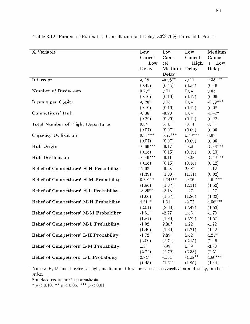
86
Table 3.12: Parameter Estimates: Cancellation and Delay, 30%-70% Threshold, Part 1
X Variable Low
Cancel
+ Low
Delay
Low
Can-
cel +
Medium
Delay
Low
Cancel
+ High
Delay
Medium
Cancel
+ Low
Delay
Intercept -0.19(0.49)
-0.95**(0.48)
-0.11(0.54)
2.35***(0.40)
Number of Businesses 0.20*(0.10)
0.01(0.10)
0.04(0.12)
0.03(0.09)
Income per Capita -0.20*(0.10)
0.05(0.10)
0.04(0.12)
-0.39***(0.08)
Competitors' Hub -0.36(0.29)
-0.29(0.29)
0.04(0.12)
-0.42*(0.22)
Total Number of Flight Departures 0.04(0.07)
0.10(0.07)
-0.14(0.09)
0.11*(0.06)
Capacity Utilization 0.33***(0.07)
0.55***(0.07)
0.49***(0.09)
0.07(0.06)
Hub Origin -0.60***(0.16)
-0.17(0.15)
-0.00(0.19)
-0.83***(0.13)
Hub Destination -0.40***(0.16)
-0.11(0.15)
-0.28(0.18)
-0.49***(0.12)
Belief of Competitors' H-H Probability -2.08(1.39)
-0.23(1.30)
2.68*(1.51)
-1.12(0.92)
Belief of Competitors' H-M Probability 6.89***(1.86)
4.84***(1.87)
-0.86(2.31)
4.01***(1.52)
Belief of Competitors' H-L Probability -3.25**(1.60)
-2.18(1.57)
1.27(1.86)
-1.57(1.32)
Belief of Competitors' M-H Probability 4.81**(2.01)
1.01(2.03)
-2.72(2.42)
4.56***(1.53)
Belief of Competitors' M-M Probability -1.51(1.87)
-2.77(1.89)
1.45(2.22)
-1.73(1.57)
Belief of Competitors' M-L Probability -1.92(1.40)
2.30*(1.39)
0.22(1.71)
-1.22(1.12)
Belief of Competitors' L-H Probability -1.72(3.00)
2.89(2.71)
2.42(3.15)
4.25*(2.49)
Belief of Competitors' L-M Probability 1.33(2.72)
0.99(2.72)
0.39(3.33)
-3.80(2.51)
Belief of Competitors' L-L Probability 2.84**(1.45)
-1.54(1.51)
-4.08**(1.90)
4.60***(1.44)
Notes: H, M and L refer to high, medium and low, presented as cancellation and delay, in thatorder.Standard errors are in parenthesis.* p < 0.10. ** p < 0.05. *** p < 0.01.

87
Table 3.13: Parameter Estimates: Cancellation and Delay, 30%-70% Threshold, Part 2
X Variable Medium
Can-
cel +
Medium
Delay
Medium
Cancel
+ High
Delay
High
Cancel-
lation
+ Low
Delay
High
Can-
cella-
tion +
Medium
Delay
Intercept 1.95***(0.39)
1.85***(0.40)
0.46(0.53)
-0.06(0.45)
Number of Businesses -0.05(0.08)
0.11(0.09)
-0.14(0.10)
0.06(0.09)
Income per Capita -0.44***(0.08)
-0.36***(0.08)
-0.29***(0.10)
-0.12(0.09)
Competitors' Hub -0.13(0.10)
0.11(0.09)
0.47*(0.29)
0.06(0.09)
Total Number of Flight Departures 0.20***(0.06)
0.09(0.06)
-0.04(0.07)
0.19***(0.06)
Capacity Utilization 0.26***(0.06)
0.34***(0.06)
-0.18**(0.07)
-0.09(0.06)
Hub Origin -0.32***(0.12)
-0.26**(0.13)
-0.42***(0.16)
-0.18(0.13)
Hub Destination -0.39***(0.12)
-0.53***(0.13)
0.20(0.16)
0.07(0.13)
Belief of Competitors' H-H Probability 0.07(0.85)
-0.56(0.87)
-4.29***(1.28)
-0.10(0.88)
Belief of Competitors' H-M Probability 4.31***(1.50)
2.28(1.59)
5.60***(1.69)
3.83**(1.51)
Belief of Competitors' H-L Probability -2.39*(1.30)
0.30(1.32)
-2.25(1.47)
-0.64(1.32)
Belief of Competitors' M-H Probability -1.06(1.54)
-3.27**(1.64)
2.62(1.77)
1.64(1.68)
Belief of Competitors' M-M Probability -1.03(1.54)
0.77(1.65)
-1.55(1.91)
-2.66(1.74)
Belief of Competitors' M-L Probability -0.74(1.12)
-2.05*(1.20)
-1.61(1.33)
0.85(1.20)
Belief of Competitors' L-H Probability 6.16**(2.40)
3.72(2.56)
3.12(2.82)
2.65(2.73)
Belief of Competitors' L-M Probability 0.88(2.46)
0.09(2.66)
3.97(2.81)
1.59(2.61)
Belief of Competitors' L-L Probability 1.86(1.41)
-0.31(1.55)
0.42(1.63)
1.19(1.45)
Notes: H, M and L refer to high, medium and low, presented as cancellation and delay, in thatorder.Standard errors are in parenthesis.* p < 0.10. ** p < 0.05. *** p < 0.01.
88
the focal rm is inclined to provide medium cancellation and low delay services, but not
inclined to provide medium cancellation and high delay services. These results again reect
the quality dierentiation in competition: rms would like to provide services better than
competitors' in some dimension (i.e., medium cancellation and low delay, as opposed to
medium cancellation and high delay), but not exactly the same service as competitors (i.e.,
avoid the medium cancellation and high delay services, which are oered by the competi-
tors). Competitors' probability of providing medium cancellation and low delay decreases
the focal rm's probability of providing medium cancellation and high delay services. This
eect suggests that when competitors are good at decreasing delay and not bad at reducing
cancellation, the focal rm is not likely to match the cancellation level with the competitor
but keeping a high delay level, compared to providing poor services in both dimensions (high
cancellation and high delay).
The probability of competitors providing low cancellation and high delay services in-
creases the likelihood of the focal rm providing medium cancellation and medium delay
services. This result suggests some horizontal quality dierentiation pattern; that is, when
competitors are doing well in one dimension of the service but bad in the other, the focal
rm is likely to not doing bad in both dimensions. By oering a dierent service package, the
focal rm attracts passengers who do not like the service package provided by competitors.
When competitors provide very good services (i.e., low cancellation and low delay), the focal
rm is likely to provide medium cancellation and low delay services, but not likely to provide
low cancellation and high delay services. This is the new insight generated by the estimation
of trichotomized service quality: the high service quality of competitors does give incentives
for the focal rm to improve their services to a level that is close to the competitors (i.e.,
medium cancellation and low delay, as opposed to low cancellation and low delay). However,
rms are more likely to decrease delay than cancellation when they are not able to decrease
both, which is reected by the negative eects of competitors' probability of providing low
cancellation and low delay services on focal rm's probability of providing low cancellation
and high delay services. This is consistent with the discussions in 3.7.1 and 3.7.2: when
rms are pressured by service competition, they are likely to decrease delay rather than
cancellation. Overall, the estimation results with trichotomized service quality levels con-
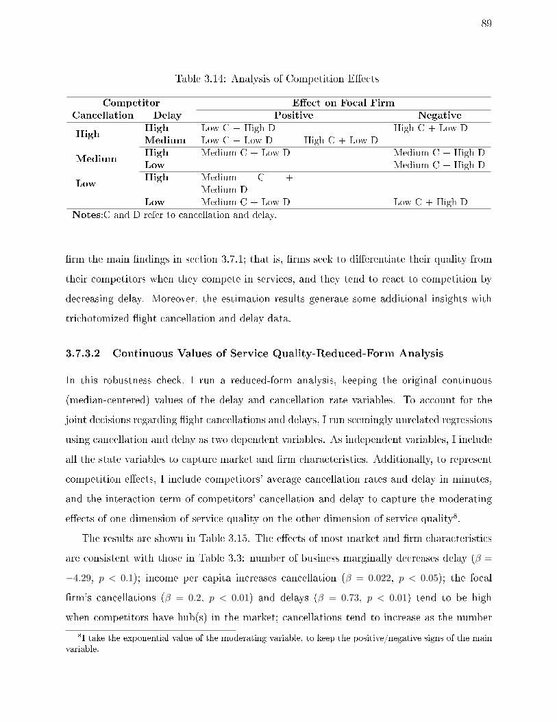
89
Table 3.14: Analysis of Competition Eects
Competitor Eect on Focal Firm
Cancellation Delay Positive Negative
HighHigh Low C + High D High C + Low DMedium Low C + Low D High C + Low D
MediumHigh Medium C + Low D Medium C + High DLow Medium C + High D
LowHigh Medium C +
Medium DLow Medium C + Low D Low C + High D
Notes:C and D refer to cancellation and delay.
rm the main ndings in section 3.7.1; that is, rms seek to dierentiate their quality from
their competitors when they compete in services, and they tend to react to competition by
decreasing delay. Moreover, the estimation results generate some additional insights with
trichotomized ight cancellation and delay data.
3.7.3.2 Continuous Values of Service Quality-Reduced-Form Analysis
In this robustness check, I run a reduced-form analysis, keeping the original continuous
(median-centered) values of the delay and cancellation rate variables. To account for the
joint decisions regarding ight cancellations and delays, I run seemingly unrelated regressions
using cancellation and delay as two dependent variables. As independent variables, I include
all the state variables to capture market and rm characteristics. Additionally, to represent
competition eects, I include competitors' average cancellation rates and delay in minutes,
and the interaction term of competitors' cancellation and delay to capture the moderating
eects of one dimension of service quality on the other dimension of service quality8.
The results are shown in Table 3.15. The eects of most market and rm characteristics
are consistent with those in Table 3.3: number of business marginally decreases delay (β =
−4.29, p < 0.1); income per capita increases cancellation (β = 0.022, p < 0.05); the focal
rm's cancellations (β = 0.2, p < 0.01) and delays (β = 0.73, p < 0.01) tend to be high
when competitors have hub(s) in the market; cancellations tend to increase as the number
8I take the exponential value of the moderating variable, to keep the positive/negative signs of the mainvariable.
90
of ight departures increases (β = 0.88, p < 0.01); cancellations tend to decrease as capacity
utilization increases (β = −3.52, p < 0.01); rms have more cancellations (β = 0.12, p < 0.01)
and delays (β = 0.82, p < 0.01) when the origin airport is a hub.
In terms of competition eects, the main results are also consistent with previous ndings.
I nd that the focal rm's cancellation is inuenced by competitors' cancellation (β = 0.15,
p < 0.01) but not by competitors' delay or the interaction term of competitors' cancellation
and delay; whereas the focal rm's delay is inuenced by competitors' delay (β = 1.88,
p < 0.05), competitors' cancellation (β = 0.11, p < 0.05), and the interaction term (β =
−1.74, p < 0.05). This result shows that rms work on their delay rather than cancellation
when they are threatened by competition, which is consistent with the results of the main
model. I also nd that the focal rm's delay decreases as competitors' delay decreases;
however, such positive impact is weakened as the competitors' cancellation decreases (the
moderating eect is negative). This result shows that rms are more likely to decrease
their delays when competitors have high service quality in only one dimension (i.e., delay or
cancellation) instead of both dimensions, which is also consistent with the results from the
main model. Overall, the robustness check generates results that are qualitatively consistent
with those in section 3.7.1, indicating that the main conclusions are not driven by the four-
level discretization of service quality choices.
3.8. Counterfactual Analysis: How New Entrants Drive
Incumbents to Adjust Service Quality
Using the estimation results, I conduct a counterfactual analysis for the Boston-Denver
market, where in the rst quarter of 2010, we observe the entry of Southwest Airlines. To
quantify how much the presence and choices of Southwest impact the probabilities of United
providing each service level, I calculate the probabilities of United taking each service level if
Southwest did not exist in the market in 2010 (given the parameter estimates) and compared
them with the actual probabilities (see Table 3.16).
I observe that Southwest Airlines was initially inclined to provide low cancellation but

91
Table 3.15: Results of Seemingly Unrelated Regressions of Cancellation and Delay
X Variable Cancella-
tion (%)
Delay
Intercept 0.56***(0.11)
-1.04***(0.40)
Number of Businesses (in 1,000,000) -3.50(9.90)
-4.29*(2.61)
Income per Capita (in 1,000) 0.022**(0.01)
0.05(0.03)
Competitors' Hub 0.20***(0.06)
0.73***(0.23)
Total Number of Flight Departures (in 1,000) 0.88***(0.06)
-0.17(0.22)
Capacity Utilization -3.52***(0.18)
6.21***(0.64)
Hub Origin 0.12***(0.04)
0.82***(0.14)
Hub Destination -0.01(0.04)
-0.55***(0.14)
Competitors' Cancellation 0.15***(0.01)
0.11**(0.05)
Competitors' Delay 0.003(0.004)
1.88**(0.91)
Competitors' Cancellation*Competitors' Delay 1.14(1.51)
NA
Competitors' Delay*Competitors' Cancellation NA -1.74**(0.88)
Note: Standard errors are in parenthesis.* p < 0.10. ** p < 0.05. *** p < 0.01.
high delay services, with its probability of oering low cancellation and high delay services
being 50% on average. In response, United became more likely to provide higher service
quality: the probability of providing both low cancellation and low delay services increased
by approximately 15%-60%, while its probabilities of providing the lowest level of service
quality with high cancellation and high delay dropped by approximately 37%. Overall, I nd
evidence that United signicantly improved its service quality with the presence of Southwest
in the market.
I conduct similar counterfactual analyses for the market Denver-Minneapolis, where there
were two new entrants. The United Airlines served in this market as a monopoly rm before
2009. In the second quarter of 2009, the Southwest Airlines entered the market and I observe

92
Table 3.16: Reaction of UA to Entry of SouthwestTime Predicted L-L Prob of
UA (no Southwest)
Actual L-L Prob of UA
(Southwest)
L-L Prob of Southwest
Q1-2010 0.1968 0.3189 0.2728Q2-2010 0.1999 0.3125 0.2962Q3-2010 0.1788 0.2989 0.2593Q4-2010 0.2024 0.3274 0.2842
Time Predicted H-L Prob of
UA (no Southwest)
Actual H-L Prob of
UA (Southwest)
H-LProb of Southwest
Q1-2010 0.1954 0.3278 0.0685Q2-2010 0.1572 0.2456 0.1003Q3-2010 0.1857 0.3218 0.0680Q4-2010 0.1805 0.3000 0.0636
Time Predicted L-H Prob of
UA (no Southwest)
Actual L-H Prob of
UA (Southwest)
L-H Prob of Southwest
Q1-2010 0.2212 0.1275 0.5610Q2-2010 0.2266 0.1421 0.4468Q3-2010 0.2079 0.1248 0.5607Q4-2010 0.2127 0.1238 0.5442
Time Predicted H-H Prob of
UA (no Southwest)
Actual H-H Prob of
UA (Southwest)
H-H Prob of South-
west
Q1-2010 0.3866 0.2259 0.0977Q2-2010 0.4164 0.2998 0.1566Q3-2010 0.4276 0.2545 0.1120Q4-2010 0.4045 0.2488 0.1080
Notes: H and L refer to high and low, presented as cancellation and delay, in that order.With the presence of Southwest, United Airlines are more likely to provide better on-time perfor-mances (decreased delays).
United improved service quality, a response similar to that in the market Boston-Denver (i.e.,
the probability of providing the low cancellation, low delay service increased by 18.6% on
average, and the probability of providing the high cancellation, low delay service increased
by 34.1%) (see Table 3.17). In the rst quarter of 2010, Delta Airlines also entered this
market. Comparing this actual scenario with the counterfactual situation where Delta is
not present, we nd that United Airlines and Southwest Airlines decreased their delays
as response. However, the change in probabilities of choosing a better service quality are
signicantly smaller (less than 10%) than the changes estimated when Southwest entered.
In fact, Southwest Airlines also responded to the entry of Delta by increasing its probability
93
of providing a better service, which, given my results, decreased the motivation of United
Airlines to improve its service quality.
3.9. Discussion and Conclusion
I study how various market characteristics, rm characteristics, and competition factors drive
rms' service performance at the market level. To capture rm service performance at the
market level, I use unique combinations of ight cancellation levels and ight delay levels. I
use a static game estimation for my analysis, and conduct robustness checks by static game
estimations with dierent discretization criteria, as well as some reduced-form analysis. In
addition, I show counterfactual analyses on the market entry eects in two representative
markets.
This section is organized as follows: in section 3.9.1 I summarize the key ndings of this
paper; in section 3.9.2 I outline the contributions of this paper to the literature; in section
3.9.3 I seek to provide detailed managerial implications with the ndings, specically, I
quantify the change of competitors' service quality decisions on the shift of the focal rm's
prots; in section 3.9.4 I briey discuss the research implications for policy makers, the
research limitations of this study, and provide directions to future research.
3.9.1 Summary of Key Findings
I nd that market characteristics, rm characteristics, and competition have dierent levels
of inuence on ight cancellation and ight delay decisions, and they also drive cancella-
tion and delay decisions in an asymmetric manner. Market characteristics have some weak
eects on rms' probability of providing very good services (i.e., low cancellation and low
delay). Specically, the size of potential business customers (number of businesses) in the
market weakly increases rms' tendency to provide very good services, while the presence of
a competitors' hub airport decreases their tendency to oer good services. Firm characteris-
tics have strong impact on ight cancellation decisions: the number of ight departures and
the presence of a hub airport in the market are likely to increase ight cancellation, while
capacity utilization reduces rms' incentives to cancel ights. In service competition, rms

94
Table3.17:Reactionof
Incumbents
toNew
Entrants:Denver-Minneapolis
Time
PredictedL-L
Prob
ActualL-L
Prob
PredictedH-L
Prob
ActualH-L
Prob
UA
WN
DL
UA
WN
DL
UA
WN
DL
UA
WN
DL
Q2-2009
0.2018
NA
NA
0.1974
0.3606
NA
0.2340
NA
NA
0.3761
0.2452
NA
Q3-2009
0.1363
NA
NA
0.1702
0.3256
NA
0.3601
NA
NA
0.4327
0.2963
NA
Q4-2009
0.2012
NA
NA
0.2486
0.3922
NA
0.2645
NA
NA
0.3097
0.0946
NA
Q1-2010
0.1049
0.2310
NA
0.1104
0.2551
0.0680
0.2402
0.1100
NA
0.2500
0.2108
0.4984
Q2-2010
0.1045
0.2471
NA
0.1109
0.2748
0.0758
0.1841
0.0906
NA
0.1964
0.1044
0.4406
Q3-2010
0.0947
0.2309
NA
0.0974
0.2405
0.0855
0.2237
0.1135
NA
0.2272
0.2054
0.3761
Q4-2010
0.1086
0.2522
NA
0.1120
0.2642
0.0702
0.2200
0.1836
NA
0.2255
0.1943
0.4578
Time
PredictedL-H
Prob
ActualL-H
Prob
PredictedH-H
Prob
ActualH-H
Prob
UA
WN
DL
UA
WN
DL
UA
WN
DL
UA
WN
DL
Q2-2009
0.1589
NA
NA
0.0577
0.2306
NA
0.4053
NA
NA
0.3688
0.1637
NA
Q3-2009
0.0817
NA
NA
0.0532
0.2199
NA
0.4219
NA
NA
0.3439
0.1582
NA
Q4-2009
0.1468
NA
NA
0.0946
0.1972
NA
0.3876
NA
NA
0.3470
0.1630
NA
Q1-2010
0.2131
0.5180
NA
0.2134
0.3535
0.041
0.4418
0.1410
NA
0.4262
0.1805
0.3926
Q2-2010
0.1844
0.4816
NA
0.2142
0.4738
0.0422
0.5270
0.1807
NA
0.4784
0.1469
0.4414
Q3-2010
0.1774
0.4775
NA
0.1918
0.3386
0.0739
0.5042
0.1781
NA
0.4837
0.2155
0.4645
Q4-2010
0.1796
0.3419
NA
0.2029
0.3425
0.0398
0.4918
0.2223
NA
0.4596
0.1990
0.4323
Notes:
HandLreferto
highandlow,presentedas
cancellationanddelay,in
that
order.
After
theentryof
Southwest,
United
Airlines
aremorelikely
toprovidebetteron-timeperform
ances(decreased
delays).After
theentryof
Delta,United
andSouthwestaremorelikely
toprovideon-timeperform
ances,butthe
change
inprobabilitiesofchoosingabetterservicequalityaresignicantlysm
allerthan
thechangeswhen
Southwest
entered.

95
show strong tendency to dierentiate their services from those oered by their competitors.
Moreover, rms are likely to have both horizontal dierentiation and vertical dierentiation
in services. For example, they tend to avoid providing exactly the same combination of
ight cancellation level and ight delay level as their competitors, to horizontally dierenti-
ate their services from those of their competitors. Vertical dierentiation is found in ight
delay decisions. When competitors have medium (high) level of ight delay, rms are in-
clined to have low (medium) level of ight delay. Overall, it seems that ight cancellation
decisions tend to be strongly driven by rm characteristics related to cancellation costs and
rescheduling convenience, while ight delay decisions are strongly responsive to competition
and rms tend to adjust their ight delay levels to dierentiate their services from those of
their competitors. In the counterfactual analysis, I show that a market entry indeed mo-
tivates incumbent rms motivated to improve their services; however, the extent of service
improvement of the incumbent rm also depends on the specic service levels of the new
entrant and other incumbent rms.
3.9.2 Contribution to the Literature
This study mainly contributes to the service marketing literature. Previous service marketing
literature (e.g., Lariviere, 2008; Spreng and Mackoy, 1996; Zeithaml et al., 1996) establishes
the importance of service quality on rms' market success. But we observe that not every
rm provides good services, and the same rm seems to oer dierent levels of services
in dierent markets. This seems to be inconsistent with ndings in the service marketing
literature, because all rms should provide good services if services are the key for rms'
success. This study is motivated by the complicated variations in service quality (measured
by ight cancellation and ight delay) across rms and markets. I come up with a model to
explain the service quality variation, and explicitly account for service competition. Most
service marketing papers focus on discussing the outcomes (e.g., customer retention, market
share) of improved service quality, except for a few studies discussing how rms may improve
service quality by being market oriented (Raju and Lonial, 2001), formalizing the selling
process, and/or applying a cross-functional team structure (Froehle et al., 2000), but none
of these studies account for competition. To my best knowledge, this is the rst paper that

96
introduces static game estimation (that accounts for endogenous competition eects) to the
service marketing literature, to explain rms' service quality decisions.
The ndings also enrich the service marketing literature. First, I nd that ight cancella-
tion and ight delay are asymmetrically inuenced by rm characteristics and competition.
This nding highlights the importance of treating service quality as a multi-dimensional
concept, regardless of studying the antecedents or consequences of service quality. Second,
I nd strong evidence of service quality dierentiation, both horizontally and vertically, in
the context of competition. This nding suggests that it is not always optimal for rms to
improve their services, indeed, it is benecial to improve services when there is room for
rms to horizontally dierentiate themselves from competitiors (i.e., have dierent service
competitive advantages from competitors'), and/or vertically dierentiate themselves from
competitors (i.e., it is possible to provide better services than competitiors).
3.9.3 Managerial Implication: Competitors' Service Quality Ad-
justments on the Focal Firm's Prots
This research oers some managerial implications related to when it is protable for rms to
improve their service quality and how they should react to competitive moves by adjusting
their own service quality. Specically, rms should invest service-related resources in markets
where the demand from business customers is strong, and/or there is room to dierentiate
their services from competitors'. Moreover, if rms intend to decrease ight cancellations,
ecient capacity management is critical; if rms are threatened by competitors' service
quality actions, decreasing delays is protable. These are the key managerial implications of
this paper.
In this section, I take an in-depth look at how competitors' service quality adjustments
inuence the protability of the focal rm when it provides each service quality level. I
therefore conducted two counterfactual analyses. In the two scenarios, the market consists
of a focal rm and a competitor, and the competitor initially has a 25% chance to provide
each level of service quality. Then the competitor improves its level of delay (Scenario 1)
or its level of cancellation (Scenario 2), so it has a 50% chance to provide low delay and
97
high cancellation (Scenario 1) or high delay and low cancellation (Scenario 2), a 50% chance
to provide low delay and low cancellation (Scenario 1) or low delay and low cancellation
(Scenario 2), and no chance of providing the other two levels of service. I compare the prot
change (in percentage) of the focal rm when it provides each level of service quality (prots
from high delay and high cancellation are always 0).
I am aware that other state variables also inuence the focal rm's prots, so I also
include two subcases in each scenario. First, I assume the focal rm has a high level of ight
departures and a high level of capacity utilization, and it operates between two hub airports
(denoted as strong). Second, I assume the focal rm has a low level of ight departures
and a low level of capacity utilization, and it does not operate between any hub airports
(weak). In both subcases, I assume the focal market does not contain many businesses and
experiences low state income per capita; the competitor also does not have a hub airport in
the market.
In Table 3.18, I provide the focal rm's prot percentage shifts, corresponding to the
competitors' service quality adjustments. The focal rm's prots from reducing cancellation
or delay decrease substantially if the competitor reduces its level of delay. This result emerges
because the competitor is likely to provide low delay and low cancellation service (50% of
chance), and the focal rm has a strong aversion to competing intensively with the competitor
by improving its service quality in this case. Moreover, the focal rm's prots from providing
low delay services decrease more if the focal rm is strong, rather than weak. It is more
costly for the focal rm to provide good service quality if it supplies large quantities of ights
or has a hub in the market. The negative eects of the other state variables all contribute
to prot decreases when the focal rm is strong.
If, however, the competitor reduces its level of cancellation, the focal rm's prots from
providing low delay services may increase. The prot increase is mainly caused by the good
likelihood that the competitor will provide high delay and low cancellation service (50%
of chance), which substantively increases the focal rm's prots through reduced delay.
The focal rm may even dierentiate itself from its competitor by improving its on-time
performance.
Note that I don't account for competitor's strategic reaction in Table 3.18, to show the
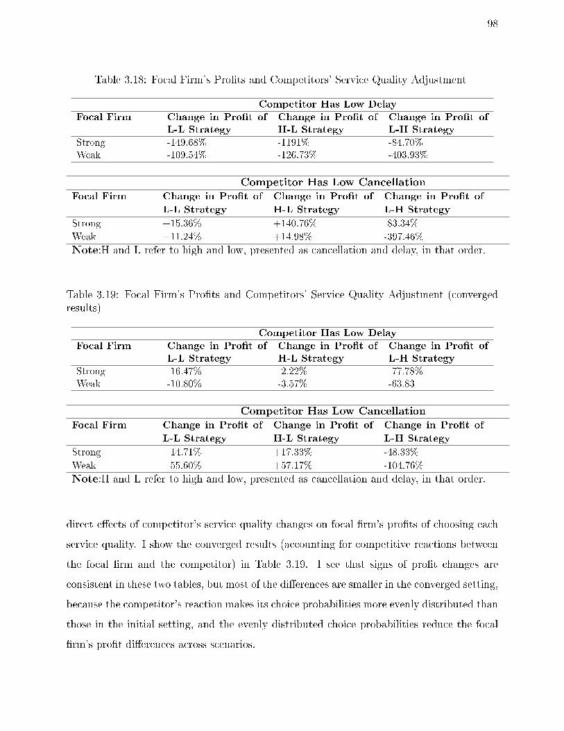
98
Table 3.18: Focal Firm's Prots and Competitors' Service Quality Adjustment
Competitor Has Low Delay
Focal Firm Change in Prot of
L-L Strategy
Change in Prot of
H-L Strategy
Change in Prot of
L-H Strategy
Strong -149.68% -1191% -84.70%Weak -109.54% -126.73% -403.93%
Competitor Has Low Cancellation
Focal Firm Change in Prot of
L-L Strategy
Change in Prot of
H-L Strategy
Change in Prot of
L-H Strategy
Strong +15.36% +140.76% -83.34%
Weak +11.24% +14.98% -397.46%
Note:H and L refer to high and low, presented as cancellation and delay, in that order.
Table 3.19: Focal Firm's Prots and Competitors' Service Quality Adjustment (convergedresults)
Competitor Has Low Delay
Focal Firm Change in Prot of
L-L Strategy
Change in Prot of
H-L Strategy
Change in Prot of
L-H Strategy
Strong -16.47% -2.22% -77.78%Weak -10.80% -3.57% -63.83
Competitor Has Low Cancellation
Focal Firm Change in Prot of
L-L Strategy
Change in Prot of
H-L Strategy
Change in Prot of
L-H Strategy
Strong +14.71% +17.33% -48.33%
Weak +55.60% +57.17% -104.76%
Note:H and L refer to high and low, presented as cancellation and delay, in that order.
direct eects of competitor's service quality changes on focal rm's prots of choosing each
service quality. I show the converged results (accounting for competitive reactions between
the focal rm and the competitor) in Table 3.19. I see that signs of prot changes are
consistent in these two tables, but most of the dierences are smaller in the converged setting,
because the competitor's reaction makes its choice probabilities more evenly distributed than
those in the initial setting, and the evenly distributed choice probabilities reduce the focal
rm's prot dierences across scenarios.

99
3.9.4 Research Implications and Future Research
In addition to the managerial implications discussed in section 3.9.3, the results also lead to
recommendations for policy makers regarding eective ways to increase overall service quality
in the industry (e.g., Tarmac Delay Rules implemented in 2010). This research suggests
some potential regulations to improve airlines' service quality: discourage rms from over-
supplying ights and/or expanding their hub cities; encourage the market entry of rms
providing good services in one dimension instead of superior services in both dimensions.
This paper enriches the services marketing literature by investigating factors that drive
rms' service quality decisions along dierent dimensions of services. There are three limi-
tations of this research. First, because of the data limitation, I use ight cancellation and
ight delay to represent service quality in the airline industry. I am aware that these two
constructs may not be sucient to capture the entire concept of service quality in this in-
dustry, such as ight attendant courtesy, availability of food and drink, etc.. Second, service
quality discretization may wash out some data variation, though the robustness checks show
that the key qualitative insights generated by the estimation are not subject to the data
discretization. Finally, the service quality of a rm might carry-over as time goes by, but we
do not account for it in this paper.
Future studies may seek to address the limitations listed above. Moreover, additional
studies can extend this research problem to other industries, such as hotels and tourism
services. It also would be interesting to incorporate rms' service recovery decisions into
the framework, to test whether service recovery decisions are inuenced by the same set of
factors as service delivery decisions.

Chapter 4
Conclusions
In this dissertation, I focus on understanding how rms make service quality decisions. In
particular, in essay I, I study how rms' service quality decisions are inuenced by the pricing
decisions and performance outcomes in the presence of competition. In essay II, I consider the
quality of two service dimensions, and explore how the focal rm's service quality decisions
(regarding to both service dimensions) are inuenced by market and rm characteristics,
and competitors' service quality decisions. Both essays nd that service quality decisions
are potentially inuenced by many factors such as prices, capacity management, demand,
and competitors' service performances. Therefore, it is not always feasible or optimal for
rms to improve their service levels.
My dissertation brings novel perspectives, in terms of data, methodology, and substantive
insights, to the services marketing literature. Whereas most existing literature largely relies
on survey data (e.g., Lariviere, 2008; Zeithaml et al., 1996), I use secondary data on service
quality (i.e., ight delays and/or ight cancellations) and other relevant variables (e.g., price,
demand, capacity) collected by Bureau of Transportation Statistics (BTS) in my dissertation.
There are a few advantages of secondary data compared to survey data. First, the secondary
data are collected monthly/quarterly since year 1993. They allow me to explore the dynamic
evolution of service quality levels and other decision or outcome variables of most major
rms (e.g., United Airlines, Delta Airlines). In my essay I, I come up with a structural
vector autoregressive panel model to assess how service quality, price, and outcome variables
drive each other dynamically, which is impossible to do with cross-sectional or two-wave
survey data. Second, because of the panel data structure, I am able to control for rm-
specic and/or market-specic xed eects in the estimations to reduce potential bias in
coecients I am interested in. It is also nearly impossible to include so many xed eects with
cross-sectional or two-wave survey data. Third, most of existing literature used subjective
measurements for service quality, which are inuenced by the perception of each individual
100

101
customer. However, rms usually cannot control customer perception; instead, it is feasible
for rms to work on objective dimensions of service quality, such as on-time performance,
facility availability, and service failure minimization. By using objective measurements for
service quality, my dissertation may generate actionable implications for rms.
My dissertation also introduces cutting-edge methodologies to services research. In essay
I, I propose a structural vector autoregressive panel model that features (1) a three-way data
structure with variables varying across rms, markets, and time; (2) a vast number of markets
(582 routes) and rms (seven airlines), such that the cross-sections of the data exceed the
time dimensions (maximum 72 quarters); (3) dependence among markets, mainly caused by
reciprocal routes; and (4) missing price information (11.41% of observations on price). To
estimate the proposed structural vector autoregressive panel model, I impute the missing
price values using missing at random specication (e.g., Little and Rubin, 1987), correct for
cross-sectional dependence between each pair of reciprocal markets (Mutl, 2009), and modify
the three-step estimation procedure suggested by Holtz-Eakin et al. (1987) to account for the
unbalanced panel structure in the data. To my best knowledge, my essay I is the rst study
using the panel vector autoregressive model to study the evolution of service quality levels.
Furthermore, I also modify the conventional Panel vector autoregressive model to account
for special features in the data (i.e., unbalanced panel structure, market dependence, missing
value). In essay II, I use the static game estimation method to account for the simultaneous
service quality decisions among competing rms in each market; i.e., the focal rm may
anticipate the service quality decisions of competing rms and determines its service quality
level accordingly. Static game estimation recently emerged in the structural econometrics
eld. To my best knowledge, my essay II is the rst paper bringing this estimation method to
services marketing literature. In summary, I believe my two essays introduce new estimation
methods to services marketing literature, and therefore provide methodological references
for future research in this domain.
My dissertation also provides substantive insights to the services marketing literature
and practices. While most previous literature discusses the potential positive outcomes of
improving service quality (e.g., Grewal et al., 2010; Rust et al., 2002), or what organizational
structures may improve service quality (e.g., Froehle et al., 2000; Raju and Lonial, 2001),

102
in my dissertation, I explore how service quality decisions of rms are inuenced by other
factors, which is a research problem not studied in previous literature. Findings of my disser-
tation suggest that it is not always feasible/optimal for rms to improve their service quality,
and service quality decisions are inuenced by factors such as prices, capacity management,
demand, and competitors' service performances. These ndings provide explanations for why
many rms do not provide good services, or not keep improving service quality. Indeed, it is
costly to provide good services, thus rms should improve their services when they are able
to achieve ecient management and increased revenue, which depend not only on service
quality but also on other decisions, such as the pricing decision. These insights are consis-
tent with those from the service prot chain literature (e.g., Heskett, Jones, man, Sasser and
Schlesinger, 1994; Raju and Lonial, 2001; Kamakura, Mittal, de Rosa and Mazzon, 2002).
Furthermore, rms do not operate independently in each market; instead, they are constantly
inuenced by their competitors. The focal rm's service quality may be perceived dierently
by customers as competitors' service quality levels vary. Firms may have incentives to oer
better services than competitors, but at the same time they need to consider the cost of pro-
viding better services than competitors. Taking the competition pressure and cost concerns
together, rms are likely to provide better services than their competitors when competitors
do not provide good services, because there is room for focal rms to improve services but
not at high costs. In sum, rms do have the tendency to vertically dierentiate their service
quality from competitors (Moorthy, 1988), conditional on that competitors are not strong in
services. In addition, given that services often include more than one dimension, rms are
also inclined to dierentiate horizontally. That is, rms tend to oer good quality in ser-
vice dimensions where competitors are weak. The insights of vertical and horizontal service
quality dierentiation are consistent with those in competition literature (e.g., de Palma, V.,
Papageorgiou and Thisse, 1985; Moorthy, 1988; Tirole, 1989; Wauthy, 1996). Findings of my
dissertation add novel insights to the services marketing literature, by bringing the concerns
of protability, feasibility, and competition into the discussion of service quality decisions.
Moreover, these insights may serve as references for service-based rms in making service
quality decisions.
In summary, my dissertation explores research problems that have not been studied

103
in extant service marketing literature, and it brings novel perspectives in terms of data,
methodology and insights. I hope my dissertation will provoke more future research in
relevant problems.

Bibliography
Ahn, S. C. and Schmidt, P. (1995), `Ecient estimation of models for dynamic panel data',
Journal of Econometrics 68(1), 527.
Anderson, E. W., Fornell, C. and Rust, R. T. (1997), `Customer satisfaction, produc-
tivity, and protability: Dierences between goods and services', Marketing Science
16(2), 129145.
Anderson, T. W. and Hsiao, C. (1982), `Formulation and estimation of dynamic models using
panel data', Journal of Econometrics 18(1), 4782.
Arellano, M. and Bond, S. (1991), `Some tests of specication for panel data: Monte carlo
evidence and an application to employment equations', Review of Economic Studies
58(2), 277297.
Bajari, P., Hong, H., Krainer, J. and Nekipelov, D. (2005), Estimating static models of
strategic interactions.
Bajari, P., Hong, H., Krainer, J. and Nekipelov, D. (2010), `Estimating static models of
strategic interactions', Journal of Business and Economics Statistics 28(4), 469482.
Ball, M. O., Homan, R., Chen, C.-Y. and Vossen, T. (2000), Collaborative decision making
in air trac management: Current and future research directions.
Baltagi, B. H. (2005), Econometric Analysis of Panel Data, John Wiley & Sons, Ltd.
Baltagi, B. H., Egger, P. and Pfaermayr, M. (2003), `A generalized design for bilateral
trade ow models', Economics Letters 80(3), 391397.
Baltagi, B. H. and Levin, D. (1986), `Estimating dynamic demand for cigarettes using panel
data: The eects of bootlegging, taxation and advertising reconsidered', Review of
Economics and Statistics 68(1), 148155.
104

105
Barnhart, S. W. and Rosenstein, S. (1998), `Board composition, managerial ownership, and
rm performance: An empirical analysis', Financial Review 33, 116.
Bergstrand, J. H. (1985), `The gravity equation in international trade: Some microeconomic
foundations and empirical evidence', Review of Economics and Statistics 67(3), 474
481.
Berry, S., Carnall, M. and Spiller, P. T. (2006), Airline Hubs: Costs, Markups and the
Implications of Customer Heterogeneity, Vol. I, Elsevier, Amsterdam and San Diego.
Berry, S., James, L. and Pakes, A. (1995), `Automobile prices in market equilibrium', Econo-
metrica 63(4), 841890.
Berry, S. and Jia, P. (2010), `Tracing the woes: An empirical analysis of the airline industry',
American Economics Review: Microeconomics 2(3), 143.
Berry, S. T. (1992), `Estimation of a model of entry in the airline industry', Econometrica:
Journal of the Econometric Society pp. 889917.
Binder, M., Hsiao, C. and Pesaran, H. M. (2005), `Estimation and inference in short panel
vector autoregressions with unit roots and conintegration', Econometric Theory 21(795-
837).
Borenstein, S. (1989), `Hubs and high fares: Dominance and market pwer in the u.s. airline
industry', RAND Journal of Economics 20(3), 344365.
Busse, M. (2002), `Firm nancial condition and airline price wars', RAND Journal of Eco-
nomics 33(2), 298318.
Centeno, M. and Vitt, U. (2011), `Chip o the old block', Ascend Contributors 2011(2), 45
49.
Chandrashekaran, M., Mehta, R., Chandrashekaran, R. and Grewal, R. (1999), `Market
motives, distinctive capabilities, and domestic inertia: A hybrid model of innovation
generation', Journal of Marketing Research 36(February), 95112.
106
Choi, I. (2001), `Unit root tests for panel data', Journal of International Money and Finance
20(249-272).
Ciliberto, F. and Williams, J. W. (2011), `Limited access to airport facilities and market
power in the airline industry', Journal of Law and Economics p. forthcoming.
Coelli, T., Grifell-Tatje, E. and Perelman, S. (2002), `Capacity utilisation and protability:
A decomposition of short-run prot eciency', International Journal of Production
Economics 79(3), 261278.
Cook, R. D. and Weisberg, S. (1994), `Transforming a response variable for linearity',
Biometrika 81(4), 731737.
Cooley, T. F. and Dwyer, M. (1998), `Business cycle analysis without much theory: A look
at structural vars', Journal of Econometrics 83(1-2), 5788.
Cornwell, C. and Trumbull, W. N. (1994), `Estimating the economic model of crime with
panel data', Review of Economics and Statistics 76(2), 360366.
Danaher, P. J. and Mattsson, J. (1994), `Customer satisfaction during the service delivery
process', European Journal of Marketing 28(5), 516.
Darmawan, I. G. N. (2002), `Norm software review: Handling missing values with multiple
imputation methods', Evaluation Journal of Australisia 2(1), 5157.
de Palma, A., V., G., Papageorgiou, Y. Y. and Thisse, J.-F. (1985), `The principle of mini-
mum dierentiation holds under sucient heterogeneity', Econometrica 53(4), 767781.
de Ruyter, K., Wetzels, M., Lemmink, J. and Mattsson, J. (1997), `The dynamics of the
service delivery process: A value-based approach', International Journal of Research in
Marketing 14, 231243.
Dickey, D. A. and Fuller, W. A. (1979), `Distribution of the estimators for autoregressive time
series with a unit root', Journal of American Statistical Association 74(366), 427431.
Egger, P. (2000), `A note on the proper specication of the gravity equation', Economics
Letters 66(1), 2531.
107
Egger, P. and Pfaermayr, M. (2003), `The propoer panel econometric specication of the
gravity equation: A three-way model with bilateral interaction eects', Empirical Eco-
nomics 28(3), 571580.
Ellickson, P. B. and Misra, S. (2008), `Supermarket pricing strategies', Marketing Science
27(5), 811828.
Enders, W. (2004), Applied Econometric Time Series, Wiley, Hoboken, NJ.
Evans, W. N. and Kessides, I. N. (1993), `Localized market power in the u.s. airline industry',
Review of Economics and Statistics 75(1), 6675.
Froehle, C. M., Roth, A. V., Chase, R. B. and Voss, C. (2000), `Antecedents of new service
development eectiveness: An exploratory examination of strategic operations choices',
Journal of Service Research 3(1), 317.
Gerardi, K. S. and Shapiro, A. H. (2009), `Does competition reduce price dispersion? new
evidence from the airline industry', Journal of Political Economy 117(1), 137.
Gopalakrishnan, B. and Johnson, E. L. (2005), `Airline crew scheduling: State-of-the-art',
Annals of Operations Research 140, 305337.
Grewal, R., Chandrashekaran, M. and Citrin, A. V. (2010), `Customer satisfaction hetero-
geneity and shareholder value', Journal of Marketing Research 48(4), 612626.
Hamilton, J. D. (1994), Time Series Analysis, Cambridge University Press.
Hartmann, W. R. (2010), `Demand estimation with social interactions and the implications
for targeted marketing', Marketing Science 29(4), 585601.
Hastings, J. (2004), `Vertical relationships and competition in gasoline markets', American
Economic Review 94(1), 317328.
Heskett, J. L., Jones, T. O., man, G. W., Sasser, W. E. J. and Schlesinger, L. A. (1994),
`Putting the service-prot chain to work', Harvard Business Review March-April.

108
Homan, R., Lee, C.-G., Ramasamy, B. and Yeung, M. (2005), `Fdi and pollution: A granger
causality test using panel data', Journal of International Development 17(3), 311317.
Holtz-Eakin, D., Newey, W. and Rosen, H. S. (1987), Wages and hours: Estimating vector
autoregressions with panel data.
Holtz-Eakin, D., Newey, W. and Rosen, H. S. (1988), `Estimating vector autoregressions
with panel data', Econometrica 56(6), 13711395.
Hoyt, D., O'Reilly, C., Rao, H. and Sutton, R. (2010), `Jetblue airways: A new beginning',
Stanford Graduate School of Business Case L-17 .
Hsiao, C., Pesaran, H. M. and Tahmiscioglu, K. A. (2002), `Maximum likelihood estimation
of xed eects dynamic panel data models covering short time periods', Journal of
Econometrics 109(1), 107150.
Huang, X. (2008), `Panel vector autoregression under cross-sectional dependence', Econo-
metrics Journal 11(2), 219243.
Ingram, P., Yue, L. Q. and Rao, H. (2010), `Trouble in store: Probes, protests, and store
openings by wal-mart, 199820071', American Journal of Sociology 116(1), 5392.
Iyer, G. and Seetharaman, P. B. (2005), Quality and location in retail gasoline markets.
Jou, R.-C., Lam, S.-H., Hensher, D. A., Chen, C.-C. and Kuo, C.-W. (2008), `The eect of
service quality and price on international airline competition', Transportation Research
Part E 44, 580592.
Kamakura, W. A., Mittal, V., de Rosa, F. and Mazzon, J. A. (2002), `Assessing the service
prot chain', Marketing Science 21(3), 294317.
Kim, E. H. and Singal, V. (1993), `Mergers and market power: Evidence from the airline
industry', American Economics Review 83(3), 549569.
Lariviere, B. (2008), `Linking perceptual and behavioral customer metrics to multiperiod
customer protability: A comprehensive service-prot chain application', Journal of
Service Research 11(1), 321.

109
Lecraw, D. J. (1978), `Determinants of capacity utilization by rms in less developed coun-
tries', Journal of Development Economics 5(2), 139153.
Levine, M. E. (2009), `Airport congestion: When theory meets reality', Yale Journal of
Regulation 26(1), 3788.
Little, R. J. A. and Rubin, D. B. (1987), Statistical Analysis with Missing Data, Wiley-
Interscience.
Love, I. and Zicchino, L. (2006), `Financial development and dynamic investment behavior:
Evidence from panel var', Quarterly Review of Economics and Finance 46, 190210.
Lundberg, S. (1985), `Tied wage-hours oers and the endogeneity of wages', Review of Eco-
nomics and Statistics 67(3), 405410.
Mazzeo, M. J. (2002), `Product choice and oligopoly market structure', RAND Journal of
Economics 33(2), 221242.
Mazzeo, M. J. (2003), `Competition and service quality in the u.s. airline industry', Review
of Industrial Organization 22, 275296.
McKelvey, R. D. and Palfrey, T. R. (1995), `Quantal response equilibria for normal form
games', Games and Economic Behavior 10(1), 638.
Mittal, V., Kamakura, W. A. and Govind, R. (2004), `Geographic patterns in customer
service and satisfaction: An empirical investigation', Journal of Marketing 68, 4862.
Moorthy, K. S. (1988), `Product and price competition in a duopoly', Marketing Science
7(2), 141168.
Morrison, S. A. and Winston, C. (1996), `Causes and consequences of airline fare wars',
Brookings Papers on Economic Activity: Microeconomics 1996, 85131.
Mutl, J. (2009), Panel var models with spatial dependence.
110
Pan, X., Ratchford, B. T. and Shankar, V. (2002), `Can price dispersion in online mar-
kets be explained by dierences in e-tailer service quality?', Journal of the Academy of
Marketing Science 30(4), 433445.
Parasuraman, A., Berry, L. L. and Zeithaml, V. A. (1985), `A conceptual model of service
quality and its implications for future research', Journal of Marketing 49(3), 4150.
Parasuraman, A., Zeithaml, V. A. and Berry, L. L. (1988), `Servqual: A multiple-item scale
for measuring consumer perceptions of service quality', Journal of Retailing 64(1), 12
40.
Parasuraman, A., Zeithaml, V. A. and Berry, L. L. (1991), `Renement and reassessment of
the servqual scale', Journal of Retailing 67(4), 420450.
Pauwels, K. (2004), `How dynamic consumer response, company support, and company
inertia shape long-term marketing eectiveness', Marketing Science 23(4), 596610.
Pauwels, K., Hanssens, D. M. and Siddarth, S. (2002), `The long-term eect of price promo-
tions on category incidence, brand choice, and purchase quality', Journal of Marketing
Research 39(421-439).
Raju, P. S. and Lonial, S. C. (2001), `The impact of quality context and market orientation
on organizational performance in a service environment', Journal of Service Research
4(2), 140154.
Ramdas, K. and Williams, J. W. (2008), An empirical investigation into the tradeos that
impact on-time performance in the airline industry.
Rubin, D. (1976), `Inference and missing data', Biometrika 63(3), 581592.
Rupp, N. G. and Holmes, G. M. (2006), `An investigation into the determinants of ight
cancellations', Economica 73, 749783.
Rupp, N. G., Owens, D. H. and Plumly, L. W. (2006), Does Competition Inuence Airline
on-Time Performance?, Vol. 1, Elsevier B. V.

111
Rust, R. T., Danaher, P. J. and Varki, S. (2000), `Using service quality data for competitive
marketing decisions', Journal of Service Management 11(5), 438469.
Rust, R. T., Moorman, C. and Dickson, P. R. (2002), `Getting return on quality: Revenue
expansion, cost reduction, or both?', Journal of Marketing 66(4), 724.
Sappington, D. E. (2003), `The eects of incentive regulation on retail telephone service
quality in the united states', Review of Network Economics 2(4), Article 5.
Schafer, J. L. (1997), Analysis of Incomplete Multivariate Data, Chapman & Hall, New York.
Shepherd, W. G. and Brock, J. W. (2009), The Structure of the American Industry, twelth
edn, Pearson - Prentice Hall, Upper Saddle Road, NJ, chapter The Airline Industry,
pp. 235264.
Sim, K. L., Koh, H. C. and Shetty, S. (2006), `Some potential issues of service quality
reporting for airlines', Journal of Air Transport Management 12(6), 293299.
Sinnott, J. (2002), Economic eects of congestion and delay.
Snider, C. (2009), Predatory incentives and predation policy: The american airlines case.
Sohoni, M., Lee, Y.-C. and Klabjan, D. (2008), Block time estimation and robust airline
scheduling.
Spreng, R. A. and Mackoy, R. D. (1996), `An empirical examination of a model of perceived
service quality and satisfaction', Journal of Retailing 72(2), 201214.
Srinivasan, S., Leszczyc, P. L. and Bass, F. M. (2000), `Market share response and compet-
itive interaction: The impact of temporary, evolving and structural changes in prices',
International Journal of Research in Marketing 17, 281305.
Steenkamp, J.-B. E. M., Nijs, V. R., Hanssens, D. M. and Dekimpe, M. G. (2005), `Compet-
itive reactions to advertising and promotion attacks', Marketing Science 24(1), 3554.
Tirole, J. (1989), The Theory of Industrial Organization, The MIT Press, Cambridge, Mas-
sachusetts.

112
Vitorino, M. A. (2012), `Empirical entry games with complementarities: An application to
the shopping center industry', Journal of Marketing Research 42(9), 175191.
Wauthy, X. (1996), `Quality choice in models of vertical dierentiation', Journal of Industrial
Economics 44(3), 345353.
Zeithaml, V. A., Berry, L. L. and Parasuraman, A. (1996), `The behavioral consequences of
service quality', Journal of Marketing 60(2), 3146.
Zhu, T., Singh, V. and Dukes, A. (2011), `Local competition, entry, and agglomeration',
Quantitative Marketing and Economics 9(2), 129154.
Zins, A. H. (2001), `Relative attitudes and commitment in customer loyalty models:
Some experiences in the commercial airline industry', Journal of Service Management
12(3), 269294.

Appendix
Supplementary documents
In this Appendix we present descriptive gures to show patterns of our four key variables
in our data. These variables are: service quality, price, capacity utilization, and number of
passengers served. We also present the impulse response functions for capacity utilization
and number of passengers served.
113

114
Figure A.1: Time Variation in Logit Delay for Select Routes
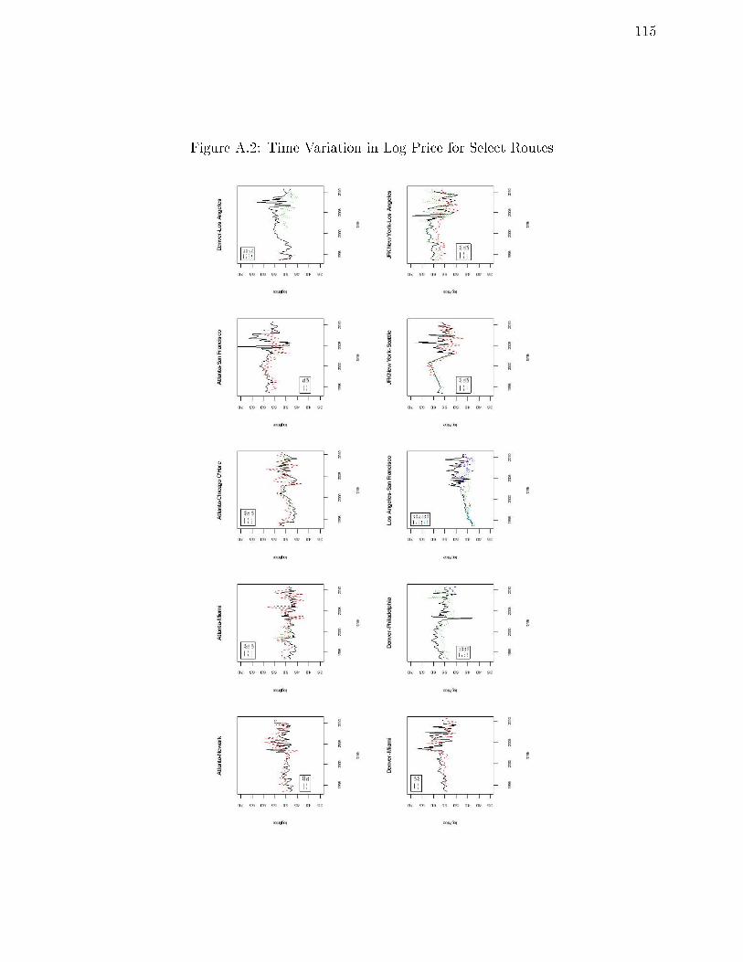
115
Figure A.2: Time Variation in Log Price for Select Routes

116
Figure A.3: Time Variation in Log Number of Passengers Served for Select Routes

117
Figure A.4: Time Variation in Logit Capacity Utilization for Select Routes

118
Figure A.5: Impact on Capacity Utilization: Impulse Response Functions
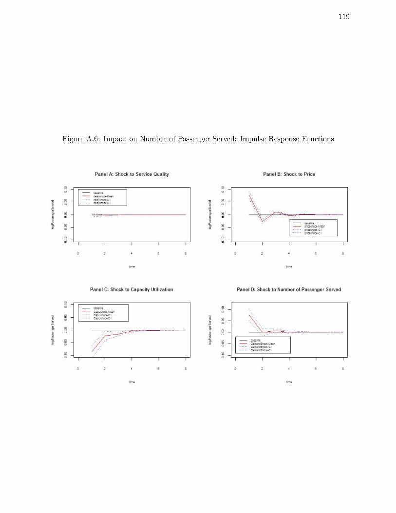
119
Figure A.6: Impact on Number of Passenger Served: Impulse Response Functions

VITA
Chen Zhou
Contact Information
485B Business Building Email: [email protected]
Department of Marketing Work: (814) 865-1825
The Smeal College of Business Cell: (814) 321-7517
The Pennsylvania State University
University Park, PA 16802
Education
• Ph.D. in Business Administration 2013 The Pennsylvania State University
• Master of Philosophy in Marketing 2008 City University of Hong Kong, Hong Kong
• B.A. in English Language and Literature 2006 Tsinghua University, China
Research Interests
Substantive Area: Service Quality Competition, Salesforce Compensation, Firm Alliance.
Methodology: Empirical Industrial Organization, Multivariate Panel Data Analysis, Econometrics.
Working Papers
• Zhou, Chen, Rajdeep Grewal and Jagmohan S. Raju, A Multi-Agent Agency Theory Model for the
Marketing-Sales Interface in Business-to-Business Firms Reject and Resubmit, under revision for
resubmission to Management Science.
• Zhou, Chen and Rajdeep Grewal, Modeling Service Quality, Price, and Performance at the Market-
Level: The Role of Potential and Realized Competition, essay 1 of my dissertation, under revision to
be submitted to Journal of Marketing Research.
• Zhou, Chen, Paulo Albuquerque and Rajdeep Grewal, A Discrete Game for Service Quality Decision
essay 2 of my dissertation, writing draft under preparation, targeted for submission toMarketing
Science.
Publications
• Yang, Zhilin, Chen Zhou and Ling Jiang (2011), When Do Formal Control and Trust Matter? A
Context-based Analysis of the Eects on Marketing Channel Relationships in China, Industrial Mar-
keting Management, 40 (1), 86-96 (revised based on the second author's master thesis).