International Journal of Environment and Resource Volume 3 Issue 2, May 2014 www.ij‐er.org
doi: 10.14355/ijer.2014.0302.02
23
Dynamic Analysis of The Hollow Jet Valve
Operation For Eutrophication Control in
Jatiluhur Tropical‐Riverine Reservoir,
Indonesia Eko W. Irianto*1, R. W. Triweko2, P. Soedjono3
1PhD Student on Water Resources Engineering, Parahyangan Catholic University, Bandung, Indonesia.
2Professor on Water Resources Engineering, Parahyangan Catholic University, Bandung, Indonesia.
3Environmental Engineering Department, Institute of Technology Bandung, Bandung, Indonesia.
[email protected]; [email protected]; [email protected]
Received 5 September 2013; Accepted 8 November 2013; Published 15 May 2014
© 2014 Science and Engineering Publishing Company
Abstract
The efforts for eutrophication control have been conducted
in many countries, i.e. physics, chemicals and biology. One
of the alternatives is hypolimnetic withdrawal technique
using hollow jet valve (HJV). So, the research objective is the
application of dynamic numerical model to analyze the affect
of HJV to reduce organics and nutrients pollutants in
Jatiluhur tropical‐riverine reservoir, Indonesia. Research
methods are as follow: (1) data collections; (2) analysis of
bathymetric maps; (3) dynamic numerical analysis using box
volume model, assisted by WASP, and (4) calibration and
simulation analyses. Results of numerical analysis shows
that HJV operation operated in at 50 m3/s, 24 hours every
month along 8 years can improve the DO, BOD, TN and TP
and chlorophyll‐a mainly in lacustrine zone, at Jatiluhur
Reservoir. Integration programs between HJV operation and
pollutant sources reduction emitted by fish‐cages
cultured,until 99% compared with existing condition can
restore Jatiluhur Reservoir from hypereutrofic to oligotrofic
statues, i.e. 3 mg/l O2; less than 0,5 mg/l BOD; 0,6 mg/l of TN;
0,05 mg/l of TP and less than 10 μg/l of Chlorophyll‐a.
Keywords
Eutrophication; WASP; Jatiluhur Reservoir; Box Volume Model;
Lacustrine Zone; Dynamic Analysis
Introduction
Background
Eutrophication condition makes several problems, i.e.
bad smelt, low of transparency and dissolved oxygen,
and toxic substances. Balcerzak (2006) explains that
eutrophication situation makes excessive growth of
phytoplankton that can absorb much DO. While, the
nitrogen fixation taken from air conducted by blue‐
green algae can cause the bed smelt and then these
conditions can reduce the ecosystem quality in
reservoir water bodies and making difficulties on
reservoir functions (Ling et al, 2007).
Efforts for eutrophication control have been conducted
in many countries. The natural control using the
predator‐fish can reduce the planktons. However, the
fish are difficult to survive in polluted condition
(Sukimin, 2004). Chemical method had been used for
eutrophication control in Wisconsin Lake, USA using
flocculants substances (Gupta and Deshora, 1977). In
spite of this, the flocculants has potency to be released
into the ecosystem. In addition, chemical‐flocculants
system is only effective to apply in small reservoir and
in the short term operation (Cooke and Denis, 1998).
Diversion channel is applied to bypass the reservoir
inflow, in order not directly discharge into reservoir
other than into the retention time pond (Suxia and
Boxin, 1991). Conversely, the method is high cost on
construction and it has potency to spread out the water
bone disease, such as schistomiasis etc (Ryding and Rast,
1989).
Artificial circulation is also used to prevent the
reservoir stratification causing the nutrients and
phytoplankton accumulation on surface layer (Hudnell
et al, 2007). Nevertheless, this technology still needs
www.ij‐er.org International Journal of Environment and Resource Volume 3 Issue 2, May 2014
24
high energy for driving the system. Sediment dredging
is also utilized for eutrophication control physically,
but it is not effective if the sedimentation problems
appeared from the reservoir catchment. Additionally,
sediment dredging method is high cost in the bottom
reservoir operation. Anaerobic conditions can make
available as well (Cook et al, (1986).
Eutrophication control technology studied above still
need energy, chemicals and high cost. With intention
that, hydrodynamics behavior initiated by reservoir
operation can be an alternative technology to reduce
the organics and nutrients generating the
eutrophication process in the reservoir. Viksburg (1995)
indicates that releasing hypolimnion water can reduce
the excessive phosphorous in the reservoir, so
eutrophication problems can be decreased.
Based on the above background, the research objective
is to apply the dynamic numerical analysis to
recognize the affect of hollow jet valve (HJV) operation
for eutrophication control in tropical‐riverine reservoir,
mainly emitted from internal pollutants load. Research
hypothesis is proper and regular operation of HJV
could affect the water quality improvement, therefore
the hypereutrophic reservoir can be restored to be
oligo‐mesotrophic reservoir in the long term operation.
Reservoir Morphometry
Chapman (1996) explains that reservoirs are formed
based on embankment in river flow. Chapman (1996)
gives details that reservoir morphometry can be
determined using Shoreline Development Index (SDI),
that can be seen at eq. 1 and Table 1.
02 *
LSDI
A (1)
SDI : Shoreline development Index
L : Length of reservoir coastal line (km)
Ao : Surface area of reservoir (km2)
Loucks, et al (2005) classify two types of reservoir
shape, i.e. regular and irregular shape. Regular shape
is often called riverine reservoir, while the other is
irregular shape, often called dendritic reservoir.
TABLE 1 RESERVOIR MORFOMETRI BASED ON SDI CRITERIA
Shape SDI
Circle type 1
Rectangle 5:1 or Elliptic type 1,5 Triangle 10:1 type ͠ ͠ ͠ 2,5
Natural lake type 2 – 5
Impoundments or Riverine type 3 – 9
Ryding and Rast (1989)
Hurtado (2006) describes that riverine reservoir has
three zones. The characteristics of each zone are: (1)
riverine zone, i.e. low retention time, high velocity,
and high nutrients concentration; (2) transition zone,
i.e. lower of velocity and higher retention time
compared to riverine zone; (3) lacustrine zone, i.e. low
nutrient and suspended solid concentrations.
Hydrodynamic conditions in riverine and transition
zone are influenced by reservoir inflow. Conversely,
lacustrine zone is affected by reservoir outflow.
Therefore, the dynamics analysis and simulation for
organics and nutrients affected by reservoir operation,
including HJV, is suitable using control volume
approach model respecting to the pollutant dynamics
in the each of segments.
Dumitran (2008) also explains that ecosystem in
lacustrine zone is affected by environmental factors,
polluted load factors and polluted load came from
upper zone of reservoir and then settling to lacustrine
zone. Gang Ji (2008) also confirms that algae and
nutrients pollutant load will concentrate to lacustrine
zone in the reservoir. For this reason, the dynamic
equations are focused in lacustrine zone on the
reservoir.
Dynamic Analysis using WASP
Nirmalakhandan (2002) explains that dynamic systems
can be relevant for investigating the environmental
problems, particularly water quality problems in
reservoir. WASP is the software of dynamic analysis to
simulate the phenomenon of pollutant transport and
transformation in the water environment and bottom
sediment (Wool dkk, 2003). The software simulates the
water quality in river, lake and reservoir using finite
difference method to accomplish the pollutant mass
equilibrium, kinetics equation and transport equation
along with the simulation time. Equations of pollutant
kinetics related to eutrophication process are follows:
(Wool et al, 2006).
(1) Phytoplankton kinetics growth:
NLTG XXXGR max (1)
RG = Phytoplankton kinetics growth
Gmax = Constants of maximum specific growth
at 200C, (0.5–4.0) per day
XT = Temperature power factor for growth (no
dimension)
XL = Light power factor for growth (no
dimension)
XN = Nutrient power factor for growth (no
dimension)
International Journal of Environment and Resource Volume 3 Issue 2, May 2014 www.ij‐er.org
25
(2) Influence of temperature to Phytoplankton :
20TT GX (2)
G = Temperature correction factor for
Growth (1.0 – 1.1)
T = Water temperature,0C
(3) Influence of light intensity to Phytoplankton :
0 0exp exp expL ee s s
I IeX t K D
K D I I
(3)
D = Mean of the depth of each segment, meter
Ke = Total light coefficient to penetrate water, per
meter
I0 = Light intensity in the surface, Langley’s/day
Is = Light saturated intensity of Phytoplankton,
Langley’s/day
(4) Phosphorous Cycle:
i Dissolved organics Phosphorous:
84
420838315
208 CCK
CkCk
t
C
mpc
TTdissdiss
(4)
Dissolution mineralization ii Dissolved An organics Phosphor:
(5)
Death mineralization growth settling
(5) Nitrogen Cycle:
i Ammonium (NH3‐N)
201 44 71 71 7
4
20 612 12 1 3 4
6
1 Tp ON nc
mpC
Tp nc NH
nit
C CD f a C k C
t k C
Ck C G a P C
K C
(6)
ii Nitrate (NO3‐N)
3
3
3
20 6212 12 1 4
6
202 2 2
6
(1 )Tp nc NH
nit
NOTD D
NO
CCk C G a P C
t K C
kk C
k C
(7)
(5) Organics (as BOD) and Dissolved Oxygen Cycle:
i Organics (as BOD):
3
3
205 6 3 51 4 5 5
6
202 2 2
6
(1 )
5 32
4 14
T s doc d D D
BOD
NOTD D
NO
C C v fa k C k C C
t k C D
kk C
k C
(8)
ii Dissolved Oxygen
3
20 206 6 62 6 5 12 12 1
6 6
20 204 1 1 4
64( )
14
32 48 32(1 )
12 14 12
T Ts D D
BOD NIT
T Ts p nc NH R R
C C Ck C C k C k C
t k C k C
SODG a P C k C
D
(9)
Methods
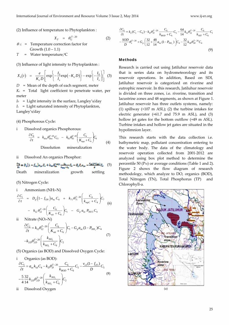
Research is carried out using Jatiluhur reservoir data
that is series data on hydrometeorology and its
reservoir operations. In addition, Based on SDI,
Jatiluhur reservoir is categorized on riverine and
eutrophic reservoir. In this research, Jatiluhur reservoir
is divided on three zones, i.e. riverine, transition and
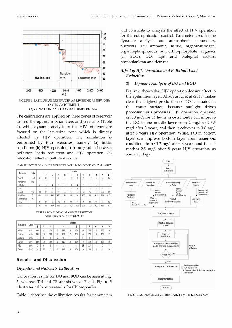
lacustrine zones and 48 segments, as shown at Figure 1.
Jatiluhur reservoir has three outlets systems, namely:
(1) spillway (+107 m ASL); (2) the turbine intakes for
electric generator (+61.7 and 75.9 m ASL), and (3)
hollow jet gates for the bottom outflow (+49 m ASL).
Turbine intakes and hollow jet gates are situated in the
hypolimnion layer.
This research starts with the data collection i.e.
bathymetric map, pollutant concentration entering to
the water body. The data of the climatology and
reservoir operation collected from 2001‐2012 are
analyzed using box plot method to determine the
percentile 50 (P50) or average conditions (Table 1 and 2).
Figure 2 shows the flow diagram of research
methodology, which analyze to DO, organics (BOD),
Total Nitrogen (TN), Total Phosphorus (TP) and
Chlorophyll‐a.
(a)
www.ij‐er.org International Journal of Environment and Resource Volume 3 Issue 2, May 2014
26
(b)
FIGURE 1. JATILUHUR RESERVOIR AS RIVERINE RESERVOIR:
(A) ITS CATCHMENT;
(B) ZONATION BASED ON BATHIMETRIC MAP
The calibrations are applied on three zones of reservoir
to find the optimum parameters and constants (Table
2), while dynamic analysis of the HJV influence are
focused on the lacustrine zone which is directly
affected by HJV operation. The simulation is
performed by four scenarios, namely: (a) initial
condition; (b) HJV operation; (d) integration between
pollution loads reduction and HJV operation; (e)
relocation effect of pollutant source.
TABLE 1 BOX PLOT ANALYSIS OF HYDRO CLIMATOLOGY DATA 2001‐2012
Parameter Units Months
J F M A M J J A S O N D
Rainfall mm/d 12 16 12 8 4 2 2 2 2 6 10 10
Windflows: m/s
Daylight 6 6 4 3 3 3 4 5 5 5 5 5
Night 3 3 2 2 2 2 3 3 3 3 3 3
Sunlight hour 3.4 3.4 3.8 5 6.5 5.2 7.2 6.4 7.2 5 3.6 3.2
Humidity % 88.4 88.8 88.2 87.2 88 88 90 90.2 91 91.2 91.8 91.2
Temperature: 0C
Min 20 20 20 20 21 21 21 20 20 20 20 20
max 32 32 32,5 32,5 32,5 32,6 32,6 32,6 32,6 32,1 32,1 32
TABLE 2 BOX PLOT ANALYSES OF RESERVOIR
OPERATIONS DATA 2001‐2012
Parameter Units Months
J F M A M J J A S O N D
Inflow m3/s 145 185 170 240 180 150 130 100 120 150 130 190
Outflow m3/s 140 110 100 140 185 185 160 180 170 160 160 175
Spillway m3/s 0 0 0 36 20 8 0 0 0 0 0 0
Turbin m3/s 140 110 100 115 125 150 150 160 150 150 150 150
HJV m3/s 0 0 0 0 18 2 18 18 2.5 4 0 0
Electric MW 90 70 65 100 115 100 100 110 100 110 95 110
Results and Discussion
Organics and Nutrients Calibration
Calibration results for DO and BOD can be seen at Fig.
3, whereas TN and TP are shown at Fig. 4. Figure 5
illustrates calibration results for Chlorophyll‐a.
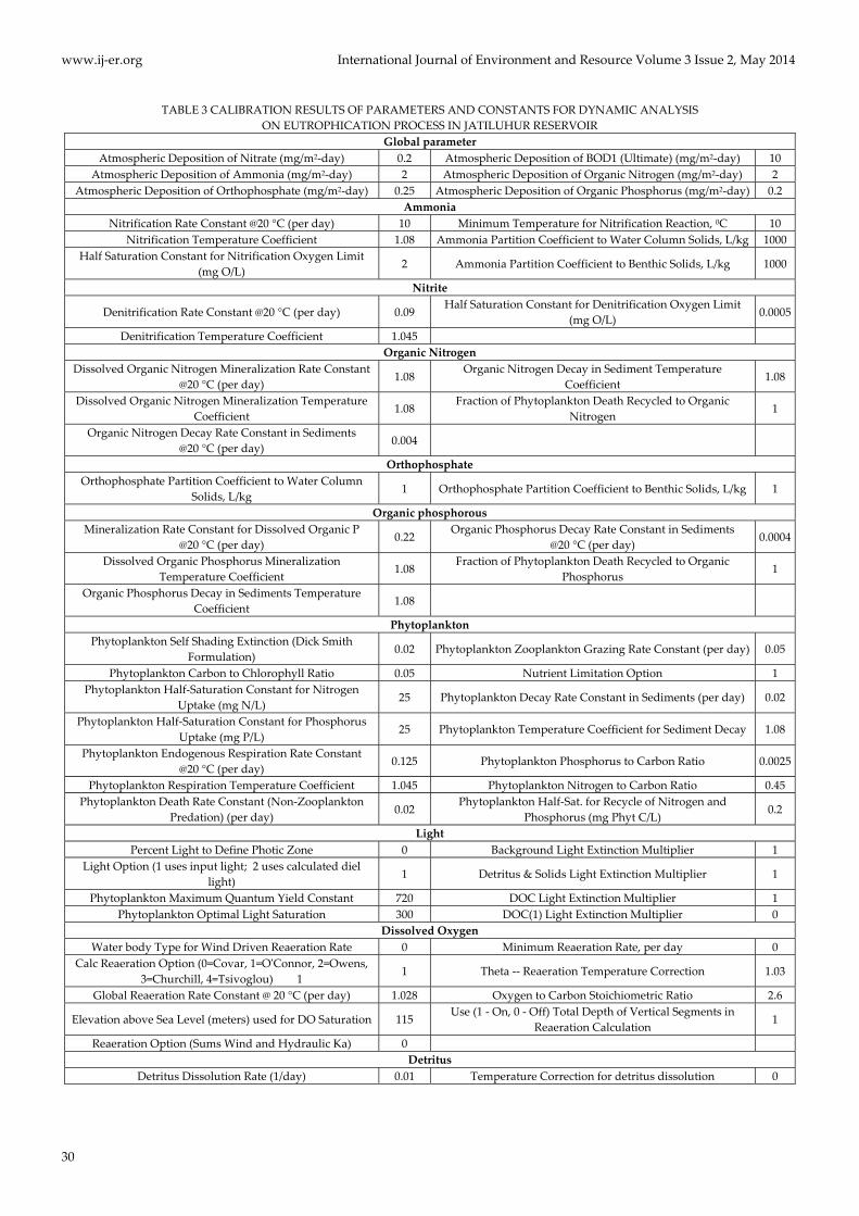
Table 1 describes the calibration results for parameters
and constants to analysis the affect of HJV operation
for the eutrophication control. Parameter used in the
dynamic analysis are atmospheric parameters,
nutrients (i.e.: ammonia, nitrite, organic‐nitrogen,
organic‐phosphorous, and ortho‐phosphate), organics
(as BOD), DO, light and biological factors:
phytoplankton and detritus
Affect of HJV Operation and Pollutant Load
Reduction
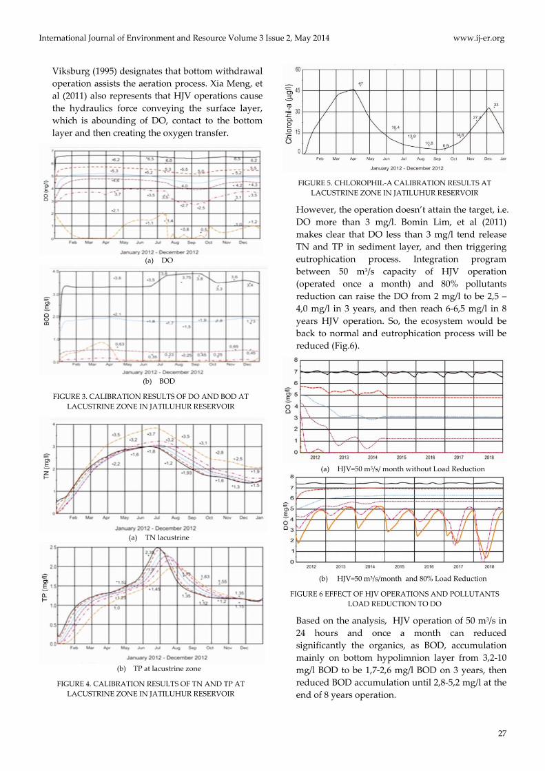
1) Dynamic Analysis of DO and BOD
Figure 6 shows that HJV operation doesn’t affect to
the epilimnion layer. Akkoyunlu, et al (2011) makes
clear that highest production of DO is situated in
the water surface, because sunlight drives
photosynthesis processes. HJV operation, operated
on 50 m3/s for 24 hours once a month, can improve
the DO in the middle layer from 2 mg/l to 2‐3.5
mg/l after 3 years, and then it achieves to 3‐8 mg/l
after 8 years HJV operation. While, DO in bottom
layer can improve bottom layer from anaerobic
conditions to be 1.2 mg/l after 3 years and then it
reaches 2.5 mg/l after 8 years HJV operation, as
shown at Fig.6.
FIGURE 2. DIAGRAM OF RESEARCH METHODOLOGY
International Journal of Environment and Resource Volume 3 Issue 2, May 2014 www.ij‐er.org
27
Viksburg (1995) designates that bottom withdrawal
operation assists the aeration process. Xia Meng, et
al (2011) also represents that HJV operations cause
the hydraulics force conveying the surface layer,
which is abounding of DO, contact to the bottom
layer and then creating the oxygen transfer.
(a) DO
(b) BOD
FIGURE 3. CALIBRATION RESULTS OF DO AND BOD AT
LACUSTRINE ZONE IN JATILUHUR RESERVOIR
(a) TN lacustrine
(b) TP at lacustrine zone
FIGURE 4. CALIBRATION RESULTS OF TN AND TP AT
LACUSTRINE ZONE IN JATILUHUR RESERVOIR
FIGURE 5. CHLOROPHIL‐A CALIBRATION RESULTS AT
LACUSTRINE ZONE IN JATILUHUR RESERVOIR
However, the operation doesn’t attain the target, i.e.
DO more than 3 mg/l. Bomin Lim, et al (2011)
makes clear that DO less than 3 mg/l tend release
TN and TP in sediment layer, and then triggering
eutrophication process. Integration program
between 50 m3/s capacity of HJV operation
(operated once a month) and 80% pollutants
reduction can raise the DO from 2 mg/l to be 2,5 –
4,0 mg/l in 3 years, and then reach 6‐6,5 mg/l in 8
years HJV operation. So, the ecosystem would be
back to normal and eutrophication process will be
reduced (Fig.6).
(a) HJV=50 m3/s/ month without Load Reduction
(b) HJV=50 m3/s/month and 80% Load Reduction
FIGURE 6 EFFECT OF HJV OPERATIONS AND POLLUTANTS
LOAD REDUCTION TO DO
Based on the analysis, HJV operation of 50 m3/s in
24 hours and once a month can reduced
significantly the organics, as BOD, accumulation
mainly on bottom hypolimnion layer from 3,2‐10
mg/l BOD to be 1,7‐2,6 mg/l BOD on 3 years, then
reduced BOD accumulation until 2,8‐5,2 mg/l at the
end of 8 years operation.
www.ij‐er.org International Journal of Environment and Resource Volume 3 Issue 2, May 2014
28
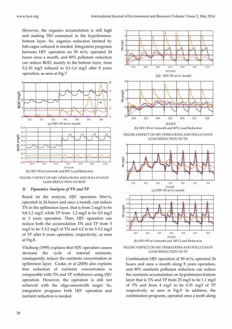
However, the organics accumulation is still high
and making DO consumed in the hypolimnion‐
bottom layer. So, organics reduction emitted by
fish‐cages cultured is needed. Integration programs
between HJV operation on 50 m3/s, operated 24
hours once a month, and 80% pollutant reduction
can reduce BOD, mainly in the bottom layer, from
5,2‐10 mg/l reduced to 0,1‐1,6 mg/l after 8 years
operation, as seen at Fig.7.
(a) HJV=50 m3/s/ month
(b) HJV=50 m3/s/month and 80% Load Reduction
FIGURE 7 EFFECT OF HJV OPERATIONS AND POLLUTANTS
LOAD REDUCTION ON BOD
2) Dynamics Analysis of TN and TP
Based on the analysis, HJV operation 50m3/s,
operated in 24 hours and once a month, can reduce
TN in the epilimnion layer, that is from 2 mg/l to be
0,8‐1,2 mg/l, while TP from 1,2 mg/l to be 0,5 mg/l
in 3 years operation. Then, HJV operation can
reduce both the accumulation TN and TP from 5
mg/l to be 3‐3.2 mg/l of TN and 4.2 to be 3‐3.2 mg/l
of TP after 8 years operation, respectively, as seen
at Fig.8.
Viksburg (1995) explains that HJV operation causes
decrease the cycle of internal nutrients,
consequently reduce the nutrients concentration in
epilimnion layer. Cooke, et al (2005) also explains
that reduction of nutrients concentration is
comparable with TN and TP withdrawn using HJV
operation. However, the operation is still not
achieved with the oligo‐mesotrofik target. So,
integration programs both HJV operation and
nutrient reduction is needed.
(a) HJV=50 m3/s/ month
(b) HJV=50 m3/s/month and 80% Load Reduction
FIGURE 8 EFFECT OF HJV OPERATIONS AND POLLUTANTS
LOAD REDUCTION TO TN
(a) HJV=50 m3/s/ month
(b) HJV=50 m3/s/month and 80% Load Reduction
FIGURE 9 EFFECT OF HJV OPERATIONS AND POLLUTANTS
LOAD REDUCTION TO TP
Combination HJV operation of 50 m3/s, operated 24
hours and once a month along 8 years operation,
and 80% nutrients pollutant reduction can reduce
the nutrients accumulation on hypolimnion‐bottom
layer that is TN and TP from 25 mg/l to be 1.1 mg/l
of TN and from 4 mg/l to be 0.35 mg/l of TP
respectively, as seen at Fig.9. In addition, the
combination programs, operated once a moth along
International Journal of Environment and Resource Volume 3 Issue 2, May 2014 www.ij‐er.org
29
8 years operation, also improve the water quality in
both of surface and middle layer that reduced the
nutrient accumulation from 5‐6 mg/l to be 0.8 mg/l
of TN and from 2.5‐4.2 mg/l to be 0.4 mg/l of TP
respectively.
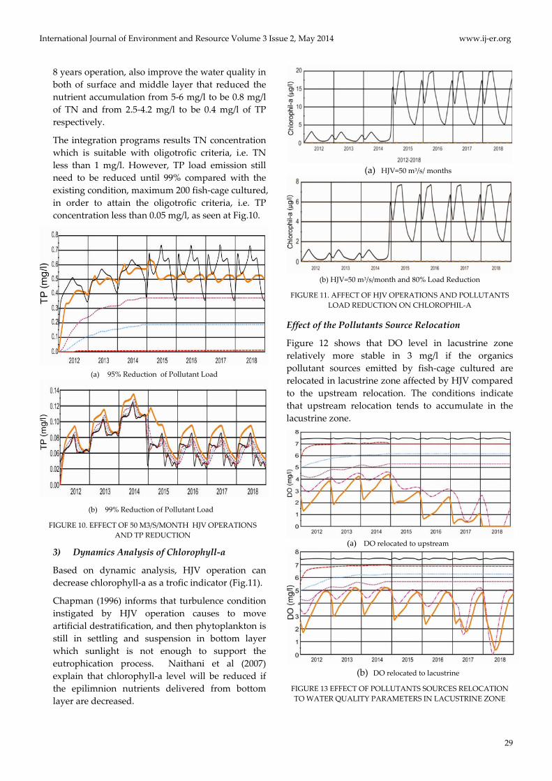
The integration programs results TN concentration
which is suitable with oligotrofic criteria, i.e. TN
less than 1 mg/l. However, TP load emission still
need to be reduced until 99% compared with the
existing condition, maximum 200 fish‐cage cultured,
in order to attain the oligotrofic criteria, i.e. TP
concentration less than 0.05 mg/l, as seen at Fig.10.
(a) 95% Reduction of Pollutant Load
(b) 99% Reduction of Pollutant Load
FIGURE 10. EFFECT OF 50 M3/S/MONTH HJV OPERATIONS
AND TP REDUCTION
3) Dynamics Analysis of Chlorophyll‐a
Based on dynamic analysis, HJV operation can
decrease chlorophyll‐a as a trofic indicator (Fig.11).
Chapman (1996) informs that turbulence condition
instigated by HJV operation causes to move
artificial destratification, and then phytoplankton is
still in settling and suspension in bottom layer
which sunlight is not enough to support the
eutrophication process. Naithani et al (2007)
explain that chlorophyll‐a level will be reduced if
the epilimnion nutrients delivered from bottom
layer are decreased.
(a) HJV=50 m3/s/ months
(b) HJV=50 m3/s/month and 80% Load Reduction
FIGURE 11. AFFECT OF HJV OPERATIONS AND POLLUTANTS
LOAD REDUCTION ON CHLOROPHIL‐A
Effect of the Pollutants Source Relocation
Figure 12 shows that DO level in lacustrine zone
relatively more stable in 3 mg/l if the organics
pollutant sources emitted by fish‐cage cultured are
relocated in lacustrine zone affected by HJV compared
to the upstream relocation. The conditions indicate
that upstream relocation tends to accumulate in the
lacustrine zone.
(a) DO relocated to upstream
(b) DO relocated to lacustrine
FIGURE 13 EFFECT OF POLLUTANTS SOURCES RELOCATION
TO WATER QUALITY PARAMETERS IN LACUSTRINE ZONE
www.ij‐er.org International Journal of Environment and Resource Volume 3 Issue 2, May 2014
30
TABLE 3 CALIBRATION RESULTS OF PARAMETERS AND CONSTANTS FOR DYNAMIC ANALYSIS
ON EUTROPHICATION PROCESS IN JATILUHUR RESERVOIR
Global parameter
Atmospheric Deposition of Nitrate (mg/m2‐day) 0.2 Atmospheric Deposition of BOD1 (Ultimate) (mg/m2‐day) 10
Atmospheric Deposition of Ammonia (mg/m2‐day) 2 Atmospheric Deposition of Organic Nitrogen (mg/m2‐day) 2
Atmospheric Deposition of Orthophosphate (mg/m2‐day) 0.25 Atmospheric Deposition of Organic Phosphorus (mg/m2‐day) 0.2
Ammonia
Nitrification Rate Constant @20 °C (per day) 10 Minimum Temperature for Nitrification Reaction, 0C 10
Nitrification Temperature Coefficient 1.08 Ammonia Partition Coefficient to Water Column Solids, L/kg 1000
Half Saturation Constant for Nitrification Oxygen Limit
(mg O/L) 2 Ammonia Partition Coefficient to Benthic Solids, L/kg 1000
Nitrite
Denitrification Rate Constant @20 °C (per day) 0.09 Half Saturation Constant for Denitrification Oxygen Limit
(mg O/L) 0.0005
Denitrification Temperature Coefficient 1.045
Organic Nitrogen
Dissolved Organic Nitrogen Mineralization Rate Constant
@20 °C (per day) 1.08
Organic Nitrogen Decay in Sediment Temperature
Coefficient 1.08
Dissolved Organic Nitrogen Mineralization Temperature
Coefficient 1.08
Fraction of Phytoplankton Death Recycled to Organic
Nitrogen 1
Organic Nitrogen Decay Rate Constant in Sediments
@20 °C (per day) 0.004
Orthophosphate
Orthophosphate Partition Coefficient to Water Column
Solids, L/kg 1 Orthophosphate Partition Coefficient to Benthic Solids, L/kg 1
Organic phosphorous
Mineralization Rate Constant for Dissolved Organic P
@20 °C (per day) 0.22
Organic Phosphorus Decay Rate Constant in Sediments
@20 °C (per day) 0.0004
Dissolved Organic Phosphorus Mineralization
Temperature Coefficient 1.08
Fraction of Phytoplankton Death Recycled to Organic
Phosphorus 1
Organic Phosphorus Decay in Sediments Temperature
Coefficient 1.08
Phytoplankton
Phytoplankton Self Shading Extinction (Dick Smith
Formulation) 0.02 Phytoplankton Zooplankton Grazing Rate Constant (per day) 0.05
Phytoplankton Carbon to Chlorophyll Ratio 0.05 Nutrient Limitation Option 1
Phytoplankton Half‐Saturation Constant for Nitrogen
Uptake (mg N/L) 25 Phytoplankton Decay Rate Constant in Sediments (per day) 0.02
Phytoplankton Half‐Saturation Constant for Phosphorus
Uptake (mg P/L) 25 Phytoplankton Temperature Coefficient for Sediment Decay 1.08
Phytoplankton Endogenous Respiration Rate Constant
@20 °C (per day) 0.125 Phytoplankton Phosphorus to Carbon Ratio 0.0025
Phytoplankton Respiration Temperature Coefficient 1.045 Phytoplankton Nitrogen to Carbon Ratio 0.45
Phytoplankton Death Rate Constant (Non‐Zooplankton
Predation) (per day) 0.02
Phytoplankton Half‐Sat. for Recycle of Nitrogen and
Phosphorus (mg Phyt C/L) 0.2
Light
Percent Light to Define Photic Zone 0 Background Light Extinction Multiplier 1
Light Option (1 uses input light; 2 uses calculated diel
light) 1 Detritus & Solids Light Extinction Multiplier 1
Phytoplankton Maximum Quantum Yield Constant 720 DOC Light Extinction Multiplier 1
Phytoplankton Optimal Light Saturation 300 DOC(1) Light Extinction Multiplier 0
Dissolved Oxygen
Water body Type for Wind Driven Reaeration Rate 0 Minimum Reaeration Rate, per day 0
Calc Reaeration Option (0=Covar, 1=OʹConnor, 2=Owens,
3=Churchill, 4=Tsivoglou) 1 1 Theta ‐‐ Reaeration Temperature Correction 1.03
Global Reaeration Rate Constant @ 20 °C (per day) 1.028 Oxygen to Carbon Stoichiometric Ratio 2.6
Elevation above Sea Level (meters) used for DO Saturation 115 Use (1 ‐ On, 0 ‐ Off) Total Depth of Vertical Segments in
Reaeration Calculation 1
Reaeration Option (Sums Wind and Hydraulic Ka) 0
Detritus
Detritus Dissolution Rate (1/day) 0.01 Temperature Correction for detritus dissolution 0
International Journal of Environment and Resource Volume 3 Issue 2, May 2014 www.ij‐er.org
31
Conclusions
Based on dynamic numerical analysis using box
volume model applied in Jatiluhur reservoir is
achieved the conclusions as follows:
a. Regular operation of HJV, operated once a month
on 50 m3/s in capacity and carried out more than 8
years operation, can improve the water quality
parameters in the reservoir that is reduction of TN
and TP initiating eutrophication process, and
reduction the organics, as BOD and then increase
the DO as an indicator of ecosystem improvement.
b. Integration program between HJV operation, 50
m3/s in capacity and carried out more than 8 years
operation, and pollutant reduction until more than
80% compared to the existing conditions can
improve the effectiveness of eutrophication control
program, particularly on fish‐cage cultured
reduction program, i.e. less than 2400 maximum of
fish‐cage cultured
c. The programs of HJV operation and pollutant
reduction can renovate the eutrophication statues
from eutrof‐hipereutrofik to be oligo‐mesotrofik,
that is DO more than 3 mg/l, BOD less than 1 mg/l,
and TN achieves less than 1 mg/l. While, attaining
TP less than 0.02 mg/l, internal pollutants should be
reduced until 99% compared with existing
conditions.
d. After reduction program, the remaining of fish‐
cage cultured should be relocated in the lacustrine
zone which is affected by the stream of HJV
outflow, compared with the upstream relocation.
Because, the pollutant emissions relocated to the
upstream in riverine zone can accumulate to the
lacustrine zone in the long time.
e. Dynamic analysis can simulate the water quality
behavior in the tropical‐riverine reservoir. The
results can also optimize the integration between
HJV operation and pollutant reduction programs to
achieve the oligotrofic level on Jatiluhur tropical‐
riverine reservoir.
ACKNOWLEDGMENT
The authors would like to thanks to Mr. Bambang
Hargono, Director of the Research and Development
Institute for Water Resources (RDIWR) Indonesia, for
all the support and also to my colleagues from Water
Environment Laboratory of RDIWR to support the
materials and data in making the research success.
REFERENCES
Akkoyunlu, A., Altun, H.Cigizoglu, H.K.2011. Depth
Integrated Estimation of DO in a Lake. J Env.Eng. 137 (10).
ASCE, pp: 961‐967.
Balcerzak, W. 2006. The Protection of Reservoir Water
against the Eutrophication Process, Institute of Water
Supply and Environmental Protection, Kraków
University of Technology, Warszawska 24, 31‐155
Kraków, Poland, Polish Jurnal of Environment Study, 15 (6),
pp 837‐844.
Bomin Lim, Bomin Ki, and Jung Hyun Choi. 2011.
Evaluation of Nutrient Release from Sediments of
Artificial Lake. J.Env.Eng. 137(5). ASCE.
Chapman, D (Editor). 1996. Water Quality Assessments ‐ A
Guide to Use of Biota, Sediments and Water in Environmental
Monitoring. Second Edition. UNESCO/WHO/UNEP,
ISBN 0 419 21590 5.
Cooke, G.D., R.T. Heath, R.H. Kennedy, and M.R. Mc Comas.
1978. Effects of Diversion and Alum Application on Two
Eutrophic Lakes. EPA‐600/3‐81‐012.
Cooke and Dennis G. 1993. Restoration and Management of
Lakes and Reservoirs, Second Edition. Lewis Publishers.
Dumitran,G.E. 2008. Bradisor Lake Restoration Affect to
Eutrophication Process. UPB Science Bulletin Series D,
70(4), Bucharest, Romania.
Gang Ji, Zhen.2008 Hydrodynamics and Water Quality:
Modelling Rivers, Lake, and Estuaries. John Willey &
Sons,Inc. New Jersey, Canada.
Gupta, R.S. and Deshora, H.S., 1977. Drinking Water Quality
Enhancement through Source Protection: Algal
Pollutants and Potable Water. Editor: Pojasek, R.B., ISBN:
0‐250‐40388‐6. Ann Arbor Science Publisher.Inc,
Michigan‐USA, pp: 431‐444.
Hoybye, J., Iritz,L., Zhlesnyak., Maderich., V., Demchenko,
Dzuba,N., Donchitz,G., Kosebutsky, V. 2002. Water
Quality Modeling to Support the Operation of the
Kakovska Reservoir, Dnieper River, Ukraine. Proceeding
of the fifth International Conference on Hydro informatics,
Cardiff, UK, IWA Publishing.
Hudnell, K., Hansen, C.K., Pattarkine, VM. 2007. Approaches
to freshwater HAB control sustainable lake water quality
restoration by inhibiting harmful algal blooms using
solar‐powered technology.

www.ij‐er.org International Journal of Environment and Resource Volume 3 Issue 2, May 2014
32
Hurtado, J.V .2006. Basin Scale Hydrodynamic in a
Mediterranean Reservoir Implications for the Phytoplankton
Ddynamics. PhD Dissertation University of Girona, Spain.
Ling, D., Wu, J. Q., Pang, Y., Li, L., Gao, G., & Hu, D. W. 2007.
Simulation study on algal dynamics based on ecological
flume experiment in Taihu Lake,China. Ecological
Engineering , 31, 200‐206. Elsevier.200‐206.
Loucks, D.P.,Van Beek, E., Stedinger, J.R., Dijkman, J. M.,
Monique T. 2005. Water Resources Systems Planning and
Management: An Introduction to Methods, Models and
Applications UNESCO, Paris.
Naithani, Darchambeau, Deleerrnijder, Descy and Wolansky.
2007. Study of the Nutrient and Plankton Dynamics in
Lake Tanganyika using a Reduced‐Gravity Model.
Ecological Modeling (200). Elsevier Science, pp: 225‐232.
Ryding dan Rast. 1989. The Control of Eutrophication of Lakes
and Reservoir. The Parthenon Publishing Group, New
York.
Sukimin. 2004. Pengelolaan Waduk Kaskade Sungai Citarum:
Tinjauan Aspek Ekologi Perairan. Seminar Pengelolaan
Waduk dan Danau, 13 Oktober 2004, Puslitbang Sumber
Daya Air, Bandung.
Viksburg, MS.1995. The WES Handbook on Water Quality
Enhancement Technique for Reservoirs and Tail waters. In
cooperation: US Army Corp of Engineers and US EPA.
Wool, A.T., Ambrose,R.B., Martin,L.J., dan E.Corner.2006.
User’s Manual:Water Quality Analysis Smulation Program
(WASP) version 6. US EPA, Atlanta.
Xia, Meng., Craig,M.P., Schaefer,B., Stoddard,A. Liu,Zhijun.,
Peng,Machuan. 2010. Influence of Phisical Forcing on
Bottom Water Dissolved Oxygen Within Caloosahtze
River Estuary. J Env.Eng, 136(10), ASCE.
Eko Winar Irianto, Bachelor on
Environmental Engineering, Institute
Technology of Bandung. Master on
Environmental Engineering, ITB,
Bandung. PhD student on Water
Resources Engineering, Parahyangan
Catholic University, Bandung, Indonesia.
Interest on water quality modeling.
Prof. Robertus Wahyudi Triweko, PhD.
Professor on Water Resources
Engineering, Parahyangan Catholic
University, Bandung, Indonesia. MEng. at
Hydraulics and Coastal Engineering,
Asian Institute of Technology, Bangkok,
Thailand. PhD on Colorado State
University, USA.
Priana Sudjono, PhD. Associate Professor
at School of Environmental Engineering,
Institute of Technology (ITB), Bandung,
Indonesia. Graduated Ph.D from
Environmental Engineering, Saga
University, Japan. Member of. Indonesian
Society of Sanitary and Environmental
Engineering.