New Jersey Institute of Technology New Jersey Institute of Technology
Digital Commons @ NJIT Digital Commons @ NJIT
Dissertations Electronic Theses and Dissertations
Spring 5-31-2012
Driver behavior classification and lateral control for automobile Driver behavior classification and lateral control for automobile
safety systems safety systems
Jing Yang New Jersey Institute of Technology
Follow this and additional works at: https://digitalcommons.njit.edu/dissertations
Part of the Electrical and Electronics Commons
Recommended Citation Recommended Citation Yang, Jing, "Driver behavior classification and lateral control for automobile safety systems" (2012). Dissertations. 303. https://digitalcommons.njit.edu/dissertations/303
This Dissertation is brought to you for free and open access by the Electronic Theses and Dissertations at Digital Commons @ NJIT. It has been accepted for inclusion in Dissertations by an authorized administrator of Digital Commons @ NJIT. For more information, please contact [email protected].

Copyright Warning & Restrictions
The copyright law of the United States (Title 17, United States Code) governs the making of photocopies or other
reproductions of copyrighted material.
Under certain conditions specified in the law, libraries and archives are authorized to furnish a photocopy or other
reproduction. One of these specified conditions is that the photocopy or reproduction is not to be “used for any
purpose other than private study, scholarship, or research.” If a, user makes a request for, or later uses, a photocopy or reproduction for purposes in excess of “fair use” that user
may be liable for copyright infringement,
This institution reserves the right to refuse to accept a copying order if, in its judgment, fulfillment of the order
would involve violation of copyright law.
Please Note: The author retains the copyright while the New Jersey Institute of Technology reserves the right to
distribute this thesis or dissertation
Printing note: If you do not wish to print this page, then select “Pages from: first page # to: last page #” on the print dialog screen

The Van Houten library has removed some of the personal information and all signatures from the approval page and biographical sketches of theses and dissertations in order to protect the identity of NJIT graduates and faculty.
ABSTRACT
DRIVER BEHAVIOR CLASSIFICATION AND LATERAL CONTROL FOR
AUTOMOBILE SAFETY SYSTEMS
by
Jing Yang
Advanced driver assistance systems (ADAS) have been developed to help drivers
maintain stability, improve road safety, and avoid potential collision. The data acquisition
equipment that can be used to measure the state and parameter information of the vehicle
may not be available for a standard passenger car due to economical and technical
limitations. This work focuses on developing three technologies (longitudinal tire force
estimation, driver behavior classification and lateral control) using low-cost sensors that
can be utilized in ADAS.
For the longitudinal tire force estimation, a low cost 1Hz positioning global
system (GPS) and a steering angle sensor are used as the vehicle data acquisition
equipment. A nonlinear extended two-wheel vehicle dynamic model is employed. The
sideslip angle and the yaw rate are estimated by discrete Kalman Filter. A time
independent piecewise optimization scheme is proposed to provide time-continuous
estimates of longitude tire force, which can be transferred to the throttle/brake pedal
position. The proposed method can be validated by the estimation results.
Driver behavior classification systems can detect unsafe driver behavior and avoid
potentially dangerous situations. To realize this strategy, a machine learning classification
method, Gaussian Mixture model (GMM), is applied to classify driver behavior. In this
application, a low cost 1Hz GPS receiver is considered as the vehicle data acquisition
equipment instead of other more costly sensors (such as steering angle sensor,
throttle/brake position sensor, and etc.). Since the driving information is limited, the
nonlinear extended two-wheel vehicle dynamic model is adopted to reconstruct the driver
behavior. Firstly, the sideslip angle and the yaw rate are calculated since they are not
available from the GPS measurements. Secondly, a piecewise optimization scheme is
proposed to reproduce the steering angle and the longitudinal force. Finally, a GMM
classifier is trained to identify abnormal driver behavior. The simulation results
demonstrated that the proposed scenario can detect the unsafe driver behavior effectively.
The lateral control system developed in this study is a look-down reference
system which uses a magnetic sensor at the front bumper to measure the front lateral
displacement and a GPS to measure the vehicle’s heading orientation. Firstly, the steering
angles can be estimated by using the data provided by the front magnetic sensor and GPS.
The estimation algorithm is an observer for a new extended single-track model, in which
the steering angle and its derivative are viewed as two state variables. Secondly, the road
curvature is determined based on the linear relationship with respect to the steering angle.
Thirdly, an accurate and real-time estimation of the vehicle’s lateral displacements can be
accomplished according to a state observer. Finally, the closed loop controller is used as a
compensator for automated steering. The proposed estimation and control algorithms are
validated by simulation results. The results showed that this lateral steering control
system achieved a good and robust performance for vehicles following or tracking a
reference path.
DRIVER BEHAVIOR CLASSIFICATION AND LATERAL CONTROL FOR
AUTOMOBILE SAFETY SYSTEMS
by
Jing Yang
A Dissertation
Submitted to the Faculty of
New Jersey Institute of Technology
in Partial Fulfillment of the Requirements for the Degree of
Doctor of Philosophy in Electrical Engineering
Department of Electrical and Computer Engineering
May 2012

ii
Copyright © 2012 by Jing Yang
ALL RIGHTS RESERVED
APPROVAL PAGE
DRIVER BEHAVIOR CLASSIFICATION AND LATERAL CONTROL FOR
AUTOMOBILE SAFETY SYSTEMS
Jing Yang
Dr. Edwin Hou, Dissertation Co-Advisor Date
Associate Professor of Electrical and Computer Engineering, NJIT
Dr. Mengchu Zhou, Dissertation Co-Advisor Date
Professor of Electrical and Computer Engineering, NJIT
Dr. Nirwan Ansari, Committee Member Date
Professor of Electrical and Computer Engineering, NJIT
Dr. Richard A. Haddad, Committee Member Date
Professor of Electrical and Computer Engineering, NJIT
Dr. Janice R. Daniel, Committee Member Date
Associate Professor of Civil and Environmental Engineering, NJIT
BIOGRAPHICAL SKETCH
Author: Jing Yang
Degree: Doctor of Philosophy
Date: May 2012
Undergraduate and Graduate Education:
• Doctor of Philosophy in Electrical Engineering,New Jersey Institute of Technology, Newark, NJ, May, 2012
• Master of Science in Automation,Tsinghua University, Beijing, P. R. China, 2006
• Bachelor of Science in Electrical and Computer Engineering,East China University of Science and Technology, Shanghai, P. R. China, 2003
Major: Electrical Engineering
Publications:
J. Yang, E. Hou and M. C. Zhou,"Front Sensor and GPS-based Lateral Control of Automated Vehicles,"Accepted for publication, IEEE Transactions on Intelligent TransportationSystems, 2012.
J. Yang, E. Hou,"Kalman Filter and GPS-based Longitudinal Tire Force Estimation,"International Journal of Intelligent Control and Systems, Vol. 16, No. 3, pp. 199-206, Sept. 2011.
J. Yang, T. N. Chang, E. Hou, and N. Ansari"Longitude Force Estimation for Bandwidth Conservative Communication andVehicular Monitoring," in Proc. of the IEEE Conference on Automation Scienceand Engineering, Toronto, Canada, pp.668- 673, 21-24 Aug. 2010.
J. Yang, T. N. Chang, and E. Hou,"Lateral Control for Vehicles' Automatic Steering with Front Sensor and GPS,"
iv
v
in Proc. of the International Conference on Control Automation and Systems,
Seoul, Korea, pp. 928-932, Oct. 2010.
J. Yang, T. N. Chang, E. Hou,
“Driver Distraction Detection for Vehicular Monitoring,”
in Proc. of the 36th Annual Conference on IEEE Industrial Electronics Society,
Glendale, AZ, USA, pp. 108-113, Nov. 2010.
J. Yang, E. Hou,
“Classification of Driving Behavior using a Gaussian Mixture Model Classifier,”
Under second round review, Proceedings of the Institution of Mechanical
Engineers, Part D, Journal of Automobile Engineering.
J. Yang, E. Hou, and M. C. Zhou,
“Driver Distraction Detection System: A Survey,”
Submitted to the IEEE Transactions on Intelligent Transportation Systems.

vi
Dedicated to my beloved parents, husband and daughter

vii
ACKNOWLEDGMENT
This dissertation would not have been possible without support, motivation and
encouragement of Dr. Timothy N. Chang. I learned many things from him and I will miss
him deeply. I especially would like to thank my advisor Dr. Edwin Hou for his guidance
and patience during my study. In particular, I want to thank my co-advisor Dr. Mengchu
Zhou for his supervision and those kind discussions with him, helping me clear my mind.
Special thanks are given to Dr. Nirwan Ansari, Dr. Richard A. Haddad, and
Dr. Janice R Daniel, for actively participating in my committee.
I would like to acknowledge the financial support provided by NJIT and National
Science Foundation Grant ECS-0823960.
Also, I want to thank all my colleagues, Biao Cheng, Lan Yu, and Wei Shi, in the
Real-time Control Laboratory for their help over the years.
Finally, I would like to thank my husband and parents for supporting and
encouraging me in everything I do.
viii
TABLE OF CONTENTS
Chapter Page
1 INTRODUCTION ...………………………………………………………………... 1
1.1 Objective ...…………………………………………………………………….. 1
1.2 Background Information……………………………………………………….. 2
1.3 Dissertation Contributions……………………………………………………... 4
1.4 Dissertation Organization …………...…………………………………………. 5
2 LITERATURE REVIEW…………………………………………………………... 7
2.1 Advanced Driver Assistance System .…………………………………………. 7
2.2 Data Acquisition Equipment...…..……………………………………………... 8
2.3 Tire Force Estimation ………………………..………………………………… 11
2.4 Vehicle States Estimation …………...………………………………………… 11
2.5 Driver Behavior Classification….…………………………………………….. 13
2.5.1 Abnormal Driver Behavior……………… …………………………….. 13
2.5.2 Driver Behavior Classification System...……………………………… 16
2.5.3 Driver Behavior Classification Algorithms…………...…………...…... 22
2.6 Lateral Control System…….…….…………………………………………….. 26
3 VEHICLE DYNAMICS………………..…………………………………………... 30
3.1 Single-track Model……………….…………………………………………….. 30
3.2 Two-wheel Extended Nonlinear Model………………….…………………….. 33
4 LONGITUDINAL TIRE FORCE ESTIMATION..………………………………... 38
4.1 Introduction……...……………….…………………………………………….. 38
4.2 Approximated Two-wheel Vehicle Dynamics...……………………………….. 40
ix
TABLE OF CONTENTS
(Continued)
Chapter Page
4.3 Sideslip Angle and Yaw Rate Estimation…......……………………………….. 42
4.4 Estimation of Longitudinal Tire Force….…......……………………………….. 45
4.5 Simulation Results….…......…………………………………………………… 48
4.5.1 Model Simulation……………………………………………………….. 48
4.5.2 Sideslip Angle and Yaw Rate Estimation..……………………………… 51
4.5.3 Longitudinal Tire Force Estimation……………………………………... 52
4.6 Summary……………………………………………………………………….. 53
5 DRIVER BEHAVIOR CLASSIFICATION……………………………………..… 54
5.1 Introduction…………..………………………………………………………… 54
5.2 Vehicle Model Simulation...…………………………………………………… 57
5.3 Sideslip Angle and Yaw Rate…………......…………………………………… 60
5.4 Piecewise of Optimization Scheme………...…...……………………………… 62
5.5 Driver Behavior Classification……….…...…………………………………… 66
5.6 Feature Extraction…………………………....………………………………… 70
5.7 Simulation Results……………………………………………………………… 71
5.8 Summary……………………………………..………………………………… 73
6 LATERAL CONTROL FOR AUTOMATED STEERING.……………………..… 75
6.1 Introduction…………..………………………………………………………… 75
6.2 Vehicle Dynamic……..………………………………………………………… 76
6.2.1 Single Track Vehicle Dynamic …………………………………………. 76
x
TABLE OF CONTENTS
(Continued)
Chapter Page
6.2.2 Actuator Dynamic ………………………………………………………. 79
6.3 State Estimation……..…………………………………………………………. 80
6.3.1 Relationship Between Road Curvature and Steering Angle...…………... 80
6.3.2 Steering Angle Estimation……………………………….....…………… 82
6.3.3 Lateral Displacement Estimation…….………………….....……………. 85
6.4 Lateral Control Design…………………………………………………………. 86
6.4.1 System Block Diagram…………………………………......…………… 86
6.4.2 Feedback Controller Structure.…………………………......…………… 88
6.5 Simulation Results…..…………………………………………………………. 90
6.6 Summary…..…………………………………………………...………………. 97
7 CONCLUSIONS AND FUTURE WORK………………….……………………… 98
7.1 Conclusions…………………………………………………………………….. 98
7.2 Future Work…...…....………………………………………………………….. 100
REFERENCES ………………………………………………………………………... 102
xi
LIST OF TABLES
Table Page
2.1 Summary of Driver Distraction Effects............................................................... 15
3.1 Notations of Two-wheel Vehicle Model.............................................................. 34
4.1 The Operation of Kalman Filter...……................................................................ 45
4.2 Values of Parameters…………...……................................................................ 48
5.1 Classification Results…………………………………………………………... 73
6.1 Parameters and Values for Vehicle Dynamic...................................................... 79
6.2 Simulation Test Cases …..…………................................................................... 91
xii
LIST OF FIGURES
Figure Page
2.1 Wheel dynamic variables………………………………………………........... 12
2.2 A general structure of driving behavior classification systems………………. 16
2.3 Throttle position when drivers are performing different in-vehicle
tasks ………………………………………………...………………………… 18
2.4 Pupil diameter ad gaze angles…..…………………………………………….. 20
2.5 Heart rate RRI in ECG wave………………………………………………….. 21
2.6 The structure of distraction mitigation system in SAVE_IT…………............. 25
2.7 Structure of lateral steering control system….…………………………........... 28
3.1 Single track model.……...…………………………………………………….
30
3.2 Nonlinear extended two-wheel vehicle model…………………………........... 33
3.3 Characteristic curve of the tires ………………………...……………….......... 36
4.1 Block diagram of the proposed method………………………………………. 46
4.2 The reference commands of model simulation….……………………………. 49
4.3(a) Noisy sampled vehicle states (velocity and yaw rate), viewed as GPS
measurements………………………………..…………………………........... 50
4.3(b) Noisy sampled vehicle states ( X and Y Coordinates), viewed as GPS
measurements…………………………………………………………………. 50
4.4 Sideslip angle and yaw rate estimation results.……………………………...... 51
4.5 Sideslip angle and yaw rate estimation error ………………………………… 51
4.6 Longitudinal tire force estimation…………………..………………………… 52
4.7 Vehicle trajectory error on the X and Y directions…………………………… 53
5.1 The reference commands of model simulation………….……………………. 57
xiii
LIST OF FIGURES
(Continued)
Figure Page
5.2 The trajectory of a left turn……………………....…………………………… 57
5.3(a) Noisy sampled vehicle states (velocity and yaw rate)…………………........... 59
5.3(b) Noisy sampled vehicle states ( X and Y coordinates)……………………….... 60
5.4 Sideslip angle and yaw rate estimation……………………………..………… 62
5.5 Steering angle and longitudinal tire force estimation………..……………….. 65
5.6 Block diagram of the proposed scheme………………..……………………... 66
6.1 Single track model including path tracking..…………………………………. 76
6.2 Block diagram of lateral steering control system using the estimations of
front and rear lateral displacement as feedback ……………………...………. 87
6.3 Implementation of the lateral control system…………………………………. 87
6.4 Actual road curvature of the reference track………….………………………. 91
6.5 Simulation results for a speed of 45mi/h on dry road ( 1µ = ) .………............. 93
6.6 Simulation results for a speed of 80mi/h on dry road ( 1µ = ) .………............. 94
6.7 Simulation results for a speed of 45mi/h on dry road ( 0.5µ = ) .……….......... 95
6.8 Simulation results for a speed of 80mi/h on dry road ( 0.5µ = ) .……….......... 96
1
CHAPTER 1
INTRODUCTION
1.1 Objective
Automobiles are ubiquitous in modern societies and they are indispensable in our daily
life. Consequently, one of the most important aspects in vehicle design by the automobile
industry is improving car safety. In the past few decades, automobile safety systems have
been developed to reduce, prevent or avoid driver error and therefore, enhanced the safety
of vehicles. These active vehicle safety systems are called advanced driver assistance
systems (ADAS).
Most applications in driver safety systems adopt multimodal sensors as the data
acquisition equipment, which may be costly and inconvenient to install for general uses.
This study aims at designing driver safety systems with low cost data acquisition
equipment to measure vehicle states (sideslip angle, yaw rate, vehicle velocity, heading
angle, and etc.), driving behavior information (steering angle and throttle/brake pedal
position), and environment data (road condition, weather condition, and other environment
conditions).
The objective of this dissertation is concentrated on developments of advanced
driver assistance systems in the following applications:
• Longitudinal tire force estimation
• Driver behavior classification
• Lateral steering control
2
1.2 Background Information
Driving safety is an important issue since driving is a common activity for many people in
everyday life. Based on the traffic statistics and analysis available from the US Department
of Transportation, Federal Highway Administration, Office of Highway Information,
during the thirty-eight years from 1970 to 2008, the number of licensed drivers in the U.S.
increased 86.82%, from about 111.5.0 million to 208.3 million. 57% of the driving-age
population was licensed to drive a motor vehicle in 1950. That number has increased to
87% of the driving-age population in 2008. Americans drove over 3 trillion miles in 2007.
From 1980 to 2005, the average annual vehicle miles traveled (VMT) per licensed driver
have increased 42.1%, from 10,043 miles to 14,273 miles [1]. Despite the safety
improvements in road and vehicle design, the total number of fatal crashes still increased.
Motor vehicle-related fatalities increased from 33,186 in 1950 to 43,510 in 2005, while the
fatality rate per 100 million vehicle miles of travel (VMT) increased from 1.46 to 7.24
[2-3]. The 2005 mortality data from the National Center for Health Statistics (NCHS)
shows the 10 leading causes of death by age group. According to the statistics, motor
vehicle traffic crashes were the leading cause of death for every group from age 3 to 34.
The motor vehicle traffic crashes ranked third overall in terms of the year of lost, behind
only to malignant neoplasms and diseases of heart [4]. The increasing number of fatalities
demonstrates that driving safety represents a persistent and important issue. Developing
advanced driver assistance systems to reduce crash involvements would benefit millions of
people across the world.
Motor-vehicle crashes can be attributed to multiple causes: driver error, road
design, vehicle design and maintenance. A 1985 study, using British and American crash
3
reports as data, found that 57% of crashes were only due to driver factors, 27% to
combined roadway and driver factors, 6% to combined vehicle and driver factors, 3%
solely to roadway factors, 3% to combined roadway, driver, and vehicle factors, 2% solely
to vehicle factors and 1% to combined roadway and vehicle factors [5]. It is obvious that
driver error represents a dominant cause of crashes. For example, driver error includes
speeding and driver impairment. On the one hand, the official British road casualty
statistics show that “traveling too fast for conditions” was a contributory factor in 11% of
all casualty-crashes [6]. On the other hand, most of the crashes are due to the impairments
of the driver’s attention. There are six major categories of attention impairments: alcohol,
fatigue, aging, physical impairment, drug use and distraction. Alcohol contributes to
approximately 40% of fatalities in US highway [7] and 33.8% of motor vehicle deaths in
Canada [8]. Accidents due to fatigues often involve young drivers and truck drivers
because they tend to adopt risky strategies such as driving at night and/or lack good-quality
sleep [7]. Old age drivers have low reaction speed and narrow field of attention [9-10].
Drivers who have poor eyesight or other physical impairment may cause fatal crashes if the
vehicle modifications are not appropriate or they are not qualified to drive. When a person
drives after using drugs (including some prescription drugs, over the counter drugs, and
illegal drugs), the potential drug impairments may create a hazardous situation to
themselves and other road uses, like pedestrians or cyclists. The last impairment is
distraction, which has become increasingly important with the introduction of in-vehicle
technologies (e.g., navigation systems, mobile phones, smart phones, and internet). Driver
distraction diverts the driver’s attention away from the activities critical for safe driving
towards a competing activity [11]. It contributes to 13-50% of all crashes, resulting in as
4
many as 10,000 fatalities and $40 billion in damages each year [7]. These statistics have
motivated research in the development of advanced driver assistance systems (ADAS).
Many ADAS have been investigated in the last decade to reduce driver error and
avoid potentially dangerous situations. The advanced driver assistance system will
enhance car safety and more generally road safety. This research is concentrated on three
applications that are the key technologies used to design advanced driver assistance
systems: longitudinal tire force estimation, driver behavior classification, and lateral
control system. Until now, most of the research and development efforts have been
dedicated to the development of these three individual technologies. For many approaches,
the vehicle and driving related information, such as steering angle, throttle/brake pedal
position, vehicle states (vehicle speed, acceleration, yaw angle, yaw rate, sideslip angle,
and etc.), distance between the ahead/flowing vehicle, are directly obtained from the
controller area network bus (CAN-bus) or multimodal sensors (GPS, steering angle sensor,
throttle/brake pedal position sensors, cameras, microphones, etc.). These data acquisition
equipment and methods are cost prohibitive and inconvenient to use for the general drivers.
This research focuses in designing three strategies: estimating longitudinal tire force,
detecting abnormal driver behavior, and automatic lateral control, by using as little
measurement devices as possible, and will therefore reduces the design cost for advanced
driver assistance systems.
1.3 Dissertation Contributions
The key contributions of this dissertation are:
1) For the vehicle state estimation, a task to estimate the longitudinal tire force
which can be transferred to the corresponding throttle/brake positions has been addressed.
5
A low cost 1Hz GPS receiver and a steering angle sensor are used as the vehicle data
acquisition equipment. A longitude force estimation scenario is developed for the
nonlinear extended two-wheel vehicle dynamic model using only the GPS information.
2) For the driver behavior classification scenario, a Gaussian Mixture model
(GMM) classifier has been developed to assign the driving behavior into normal or
abnormal category. The vehicle states and the driver inputs are estimated according to the
GPS data and the vehicle dynamic models. GMM is used to capture the sequence of driving
characteristics based on the reconstructed driver’s inputs. This application can enhance the
safety of the drivers by warning drivers in potentially dangerous traffic situations.
3) For vehicle lateral steering control, a GPS and front sensor based approach is
adopted to estimate in real time the necessary states and model parameters (the steering
angle, road curvature, and lateral displacements). The control strategy used is a look-down
reference system which uses a sensor at the front bumper to measure the lateral
displacement and a GPS to measure the heading orientation. An accurate and real-time
estimation of the lateral displacements with respect to the road can be accomplished in
such a control system. The simulation results show that the system provides a good and
robust performance for path tracking.
1.4 Dissertation Organization
The rest of this dissertation is organized as follows: Chapter 2 presents the currently
available technology and offers a review of the relevant literature. It begins with
introduction of the advanced driver assistance system. Then, data acquisition equipment
used in driver safety systems is investigated, followed by a discussion on the vehicle states
estimation and longitudinal tire force estimation. The concepts of driver behavior
6
classification approaches are also presented. Finally, the current lateral control systems are
discussed. Chapter 3 introduces two types of vehicle dynamics used in this thesis:
single-track linear model and two-wheel extended nonlinear model. Chapter 4 is dedicated
to the proposed a novel strategy to estimate longitudinal tire force for two-wheel extended
vehicle model. The state estimator is studied. In order to estimate the longitudinal tire
force, an optimizer is then developed. Chapter 5 discusses a scenario to detect the abnormal
driver behavior. The driver behavior is reconstructed and a Gaussian mixture model
classifier is used to determine whether the driver behavior is normal or abnormal. A novel
lateral steering control system with a GPS and a front sensor is presented in Chapter 6. The
entire system is a look-down system which has three parts: a road curvature and steering
angle estimator, a lateral states observer, and a feedback controller. Chapter 7 concludes
this dissertation.
7
CHAPTER 2
LITERATURE REVIEW
2.1 Advanced Driver Assistance System
In the past few decades, advanced automobile safety systems have been studied and
developed mostly in research laboratories. Only until recently, automobile manufacturers
are beginning to deploy them in the production of consumer vehicles. Automobile safety
systems can be grouped into two categories: Passive safety systems and Active safety
system.
Passive safety systems are only deployed or effective in response to an
automobile crash. These systems protect drivers and passengers from injuries or reduce
severity of injuries during the collision. Passive systems include seat belts, air bags,
headrests, and the passenger-safety cage. For example, air bags are now mandatory in
every new automobile sold in the United States. Vehicle crashworthiness is another
regulated passive system. The regulation of crashworthiness began in the late 1960s
and
today all vehicles in the U.S. are required to pass mandated crashworthiness tests before
they are sold to the public.
Advanced Driver Assistance Systems (ADAS) are active safety systems that can
reduce the possibility of crashes. They aim at providing assistance to the driver by
informing them about the condition of the car, the condition of the road, any potential
hazards, or by providing active assistance to the driver. An ADAS may include many
types of practical systems, for example, lateral control systems, longitudinal control
systems, automated highway system (AHS), driver distraction detection system, reversing
or parking aids, vision enhancements systems, and intelligent speed adaptation, in-vehicle
8
navigation system, antilock brake system, electronic stability program, collision
avoidance system, intelligent cruise control, lane departure warning system, lane change
assistance, automatic parking, intelligent speed adaptation, night vision, adaptive light
control, pedestrian protection system, traffic sign recognition, blind spot detection, driver
drowsiness detection, vehicular communication system, hill descent control, electrical
vehicle warning sounds used in hybrids and plug-in electric vehicles [12]. An overview
of longitudinal tire force estimation, driver behavior classification system and lateral
control system, which is the focuses of this study, is presented in the following sections.
2.2 Data Acquisition Equipment
An ADAS needs to measure or estimate vehicle and driving related information and
process them to automatically control the vehicle or provide feedback to the driver. These
data include steering angle, throttle/brake pedal position, vehicle states (vehicle speed,
acceleration, yaw angle, yaw rate, sideslip angle, and etc.), distance between the
ahead/flowing vehicles, and lateral displacement. The information can be obtained from
multimodal data acquisition sensors and equipment installed in the vehicle. The
commonly utilized data acquisition devices in ADAS include:
• Controller area network bus (CAN-bus)
CAN-bus is a vehicle bus standard designed to allow microcontrollers and devices
to communicate with each other. The CAN-bus is a serial, asynchronous, multi-master
communications protocol suited for networking a vehicle’s electronic control systems,
sensors, and actuators. The CAN-bus signal contains real-time vehicle information in the
form of messages integrating many modules. Usually, the open connector to the CAN-
bus is the On-Board Diagnostics (OBD-II) port. The driving parameters provided by the
9
CAN-bus usually include Revolutions per minute (RPM), Acceleration pedal position,
Wheel speeds, Steering angle, Lateral acceleration and yaw rate. Different vehicle models
may provide all or part of the above data. One of the limitations of the CAN-bus signals
is that they are not available for every vehicle models. Besides, the CAN-bus signals are
coded with standards that differ from one manufacture to another. Thus, the database
used to decode the CAN-bus signal may not be available to the general public or the cost
for the database and data acquisition software maybe prohibitive.
• Global Position System (GPS)
A GPS is used to measure the position of the vehicle, its heading orientation, and
even its vehicle velocity. Currently, a low-cost vehicle GPS has an updating rate of 1Hz
or 5Hz . In research projects conducted by various vehicle research programs (such as
DARPA Grand challenge, California PATH, Department of Transportation, and so on),
more accurate GPS (for example, absolute GPS, differential GPS, or GPS with a higher
updating rate) were employed. In order to obtain the rate up to 100 Hz, a GPS/INS is
usually adopted, where INS stands for Inertial Navigation System. It refers to the use of
GPS satellite signals to correct or calibrate a solution from an INS. INS usually can
continuously provide accurate measurements of a vehicle’s position, orientation, or
velocity.
• Steering angle sensor
The overall steering wheel angle is measured by the steering angle sensor which
is mounted on the steering shaft.
• Throttle/brake pedal position sensors

10
Throttle pedal position sensor and brake pedal position sensor are used to measure
the positions of the acceleration and brake pedal respectively.
• Yaw rate sensor
A yaw rate sensor is a gyroscopic device that measures a vehicle’s angular
velocity around its vertical axis.
• Magnetic sensor
A magnetic sensor is a distance sensor, which can be used to measure the lateral
displacement or longitudinal distance between two vehicles.
• Cameras
Video cameras can be used to record the driver’s eye, head movements, face
features, vehicle’s motions or road condition.
• Microphones
Microphones can be used to record a driver’s speech.
• Body sensors
Body sensors can provide the information about a driver’s body movements, e.g.,
hand and neck movements.
• faceLAB
faceLAB is an eye and facial tracking system developed by Seeing Machines, Inc.
[95]. It consists of a separate computer, Sony stereo cameras and loud-speakers. The
computer is used for image processing. Cameras are positioned to the left and right of
the screen above the dashboard for image capturing. It can capture the data on eye
movement, head position and rotation, eyelid aperture, lip and eyebrow.
11
2.3 Vehicle States Estimation
Knowledge of the vehicle variables is essential for advanced driver assistance systems.
However, some of the fundamental variables (such as sideslip angle, vehicle velocity,
yaw angle, yaw rate) are not measurable in a standard car due to both technical and
economical reasons. Consequently, these variables must be observed or estimated.
Among those fundamental variables, the sideslip angle and the yaw rate are of most
critical.
The vehicle sideslip angle can be calculated if the orientation (attitude) and
velocity of the vehicle are known because the sideslip angle is the difference between the
yaw angle and the direction of the velocity. For most cases when the orientation (attitude)
and velocity are not available, a number of methods have been proposed to estimate the
sideslip angle. Existing common methods can be based on dynamic handling models [21-
22], estimators that are designed according to the kinematic relationships [23], the
combined measurements of the yaw rate gyro and lateral accelerometer [24-25]. The
sideslip angle can be also estimated by the integration of the yaw rate and the lateral
acceleration because the derivative of the sideslip angle can be expressed in terms of
these measurements [26-27].
2.4 Tire Force Estimation
The tire force determines the vehicle’s motion in both lateral and longitudinal directions.
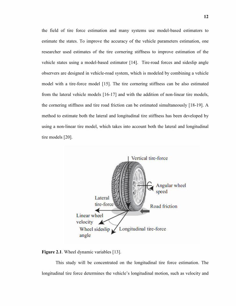
Figure 2.1 illustrates the wheel dynamic variables [13] which can be used to model the
tire force. Based on the tire model, tire force can be directly calculated by the wheel
cornering stiffness and sideslip angle. The wheel cornering stiffness is a parameter
closely related to the tire-road friction. Large amount of research have been reported in
12
the field of tire force estimation and many systems use model-based estimators to
estimate the states. To improve the accuracy of the vehicle parameters estimation, one
researcher used estimates of the tire cornering stiffness to improve estimation of the
vehicle states using a model-based estimator [14]. Tire-road forces and sideslip angle
observers are designed in vehicle-road system, which is modeled by combining a vehicle
model with a tire-force model [15]. The tire cornering stiffness can be also estimated
from the lateral vehicle models [16-17] and with the addition of non-linear tire models,
the cornering stiffness and tire road friction can be estimated simultaneously [18-19]. A
method to estimate both the lateral and longitudinal tire stiffness has been developed by
using a non-linear tire model, which takes into account both the lateral and longitudinal
tire models [20].
Figure 2.1. Wheel dynamic variables [13].
This study will be concentrated on the longitudinal tire force estimation. The
longitudinal tire force determines the vehicle’s longitudinal motion, such as velocity and
13
acceleration. Since longitudinal tire force can be transferred to the corresponding
throttle/brake positions, the driver behavior could be reconstructed.
2.5 Driver Behavior Classification
Driver behavior can be classified into either normal or abnormal behavior. Numerous
research studies have conducted to detect abnormal driver behavior. This section begins
by discussing abnormal driver behavior and then driver behavior classification systems
are introduced. Finally, currently existing abnormal driver behavior detection approaches
are discussed.
2.5.1 Abnormal Driver Behavior
Abnormal driving behavior is defined as the behavior that is influenced by either mental
or physical impairments. Six major categories of impairments are defined and they are:
alcohol, fatigue, aging, physical impairment, drug use and distraction. It has been found
that distraction represent the dominant cause of crashes [11].
The International Standards Organization developed the following definition for
distraction: Distraction is “attention given to non-driving-related activity, typically to the
detriment of driving performance” [28]. The comprehensive definition of driver
distraction is presented by the Australian Road Safety Board in 2006 [29]: “Driver
distraction is the voluntary or involuntary diversion of attention from the primary driving
tasks not related to impairment (from alcohol, drugs, fatigue, or a medical condition)
where the diversion occurs because the driver is performing an additional task (or tasks)
and temporarily focusing on an object, event, or person not related to the primary driving
tasks.” The diversion reduces a driver’s situational awareness, decision making and/or
14
performance resulting, in some instances, in a collision or near-miss or corrective action
by the driver and/or other road user.
There are three types of driver distraction when considering the different sources
that cause the driver’s inattention.
Firstly, there is a general agreement that the existence of a triggering activity is a
critical part of the definition. The triggering activity means a secondary task which
diverts the driver’s attention away from the driving task. The triggering activity can be
classified into three categories: purposeful activity (e.g., inserting a CD, texting on a cell
phone, or inputting information into navigation systems); incidental activity (e.g.,
answering a phone, interacting with passengers or eating); and uncontrolled activity (e.g.,
movement of animal and child inside the vehicle, sneezing, coughing or itching) [30].
Secondly, there is also a growing realization that “cognitive distraction” is a
significant component of driver distraction. Cognitive distraction refers to the mental
workload associated with a task (e.g., being lost in thought, emotionally upset or
emotionally preoccupied). Cognitive distraction is generally not observable [30-31] in
most situations.
Finally, external distractions are also involved in the categorizations of driver
distraction. The external distractions include unusual or unexpected events or activities
(e.g., wild animals crossing), inclusion of relatively common driving situations (e.g.,
driver blinded by sun or by oncoming headlines, sirens of police emergency vehicles),
and external objects (e.g., advertising signage, outside person objects or events) [32].
When considering the different ways that distracting tasks affect drivers, the
driver distraction can be categorized into three types [33]:
15
• Visual distraction: Tasks that require the driver to look away from the roadway to
visually obtain information;
• Manual distraction: Tasks that require the driver to take a hand off the steering
wheel and manipulate a device;
• Cognitive distraction: Tasks that require mental workload so that the driver will
be thinking about something other than the driving task.
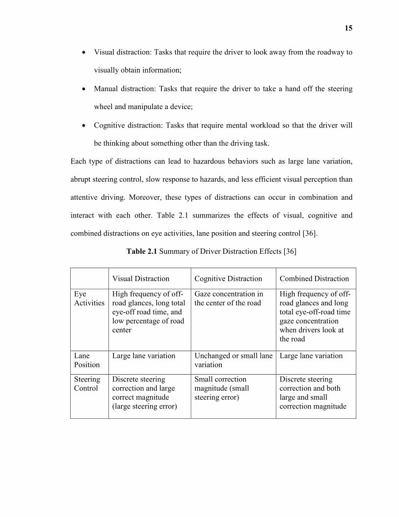
Each type of distractions can lead to hazardous behaviors such as large lane variation,
abrupt steering control, slow response to hazards, and less efficient visual perception than
attentive driving. Moreover, these types of distractions can occur in combination and
interact with each other. Table 2.1 summarizes the effects of visual, cognitive and
combined distractions on eye activities, lane position and steering control [36].
Table 2.1 Summary of Driver Distraction Effects [36]
Visual Distraction Cognitive Distraction Combined Distraction
Eye
Activities
High frequency of off-
road glances, long total
eye-off road time, and
low percentage of road
center
Gaze concentration in
the center of the road
High frequency of off-
road glances and long
total eye-off-road time
gaze concentration
when drivers look at
the road
Lane
Position
Large lane variation Unchanged or small lane
variation
Large lane variation
Steering
Control
Discrete steering
correction and large
correct magnitude
(large steering error)
Small correction
magnitude (small
steering error)
Discrete steering
correction and both
large and small
correction magnitude
16
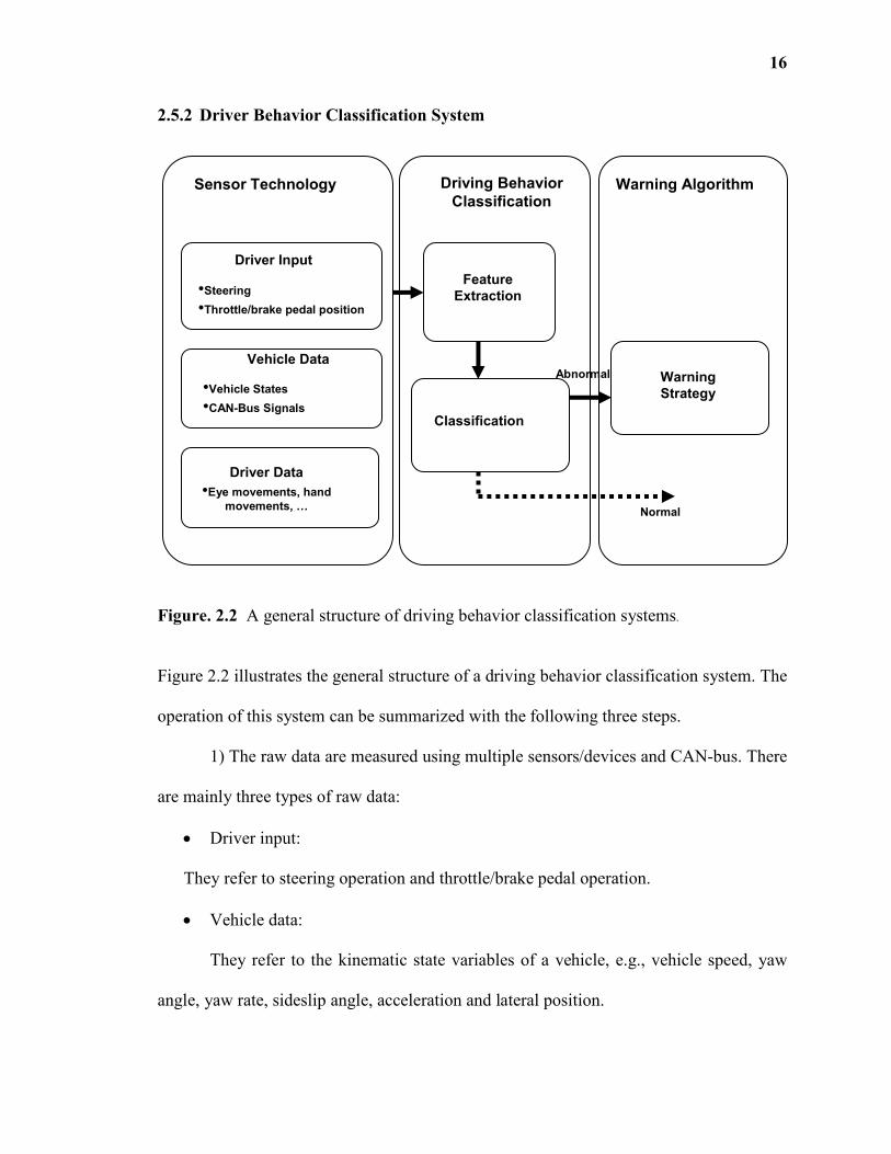
2.5.2 Driver Behavior Classification System
Figure. 2.2 A general structure of driving behavior classification systems.
Figure 2.2 illustrates the general structure of a driving behavior classification system. The
operation of this system can be summarized with the following three steps.
1) The raw data are measured using multiple sensors/devices and CAN-bus. There
are mainly three types of raw data:
• Driver input:
They refer to steering operation and throttle/brake pedal operation.
• Vehicle data:
They refer to the kinematic state variables of a vehicle, e.g., vehicle speed, yaw
angle, yaw rate, sideslip angle, acceleration and lateral position.
Sensor Technology
Driving Behavior
Classification
Feature
Extraction
Classification
Warning
Strategy
Warning Algorithm
Normal
Driver Data
•Eye movements, hand
movements,
Vehicle Data
•Vehicle States
•CAN-Bus Signals
Driver Input
•Steering
•Throttle/brake pedal position
Abnormal
17
• Driver data:
They refer to the driver behaviors and reactions, like eye movement, head
movement, hand movement, body movement or physiological response.
2) Certain features of the data are extracted and used to represent the driving
behavior. These features are then used to classify the driver’s state. For most system,
there are two states: normal driving behavior and abnormal driving behavior. The
decision whether a driver behavior is abnormal or not can be determined according to
some rules (e.g., a classification approach or a classifier) based on these features.
Prior studies have reported various features that can be used to measure the level
of driver’s abnormality. They indicated the effects of distraction on the driver’s inputs,
vehicle state information and driver’s behavior.
• Driver control input features:
Some researchers have adopted statistics of a driver’s operation signals to
measure the driving performance. It was found that the mean, variance, root mean square
(RMS) and entropy of steering angles are suitable to reflect a driver’s steering maneuvers
[89, 92-93]. It was pointed out in [90] and [91] that driver distractions may cause a
delayed accelerator release reaction time. This delayed accelerator release reaction time is
defined as the time when the lead vehicle starts to brake until the driver releases the
accelerator. In the UMTRI research in the SAVE-IT project, it was found that when
drivers are performing an in-vehicle task, they control their speed by intermittently
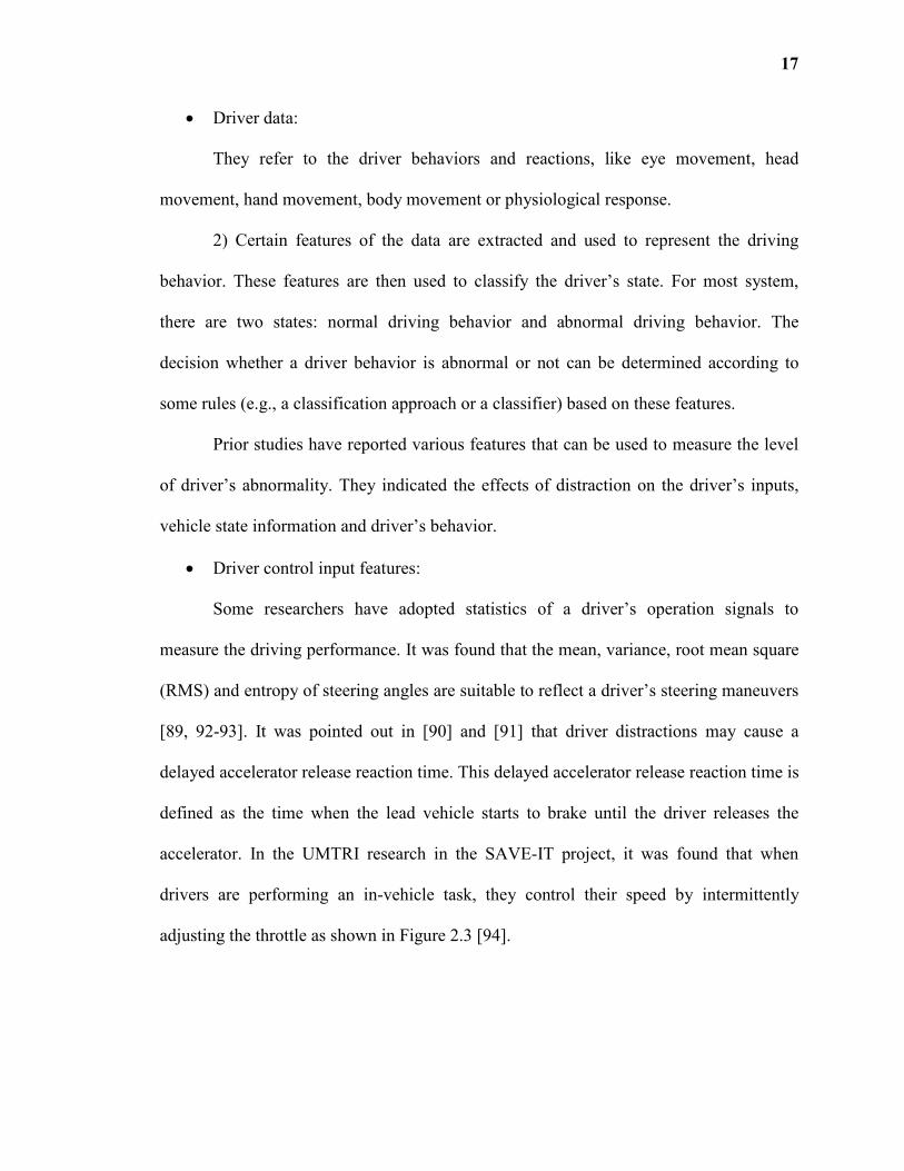
adjusting the throttle as shown in Figure 2.3 [94].
18
Figure 2.3 Throttle position when drivers are performing different in-vehicle tasks [94].
• Vehicle kinematic state features:
Driver abnormal behavior is associated with unintended changes of a vehicle’s
state resulting in unsafe driving performance. The vehicle state includes forward speed,
lane position, sideslip angle, yaw angle, and yaw rate. Ranney [96] found that distraction
may result in speed changes or allowing the vehicle to drift outside the lane boundaries.
Zylstra et al. [97] point out that distracted driving does affect the mean lateral position. It
was shown in [98] that the standard deviation of lane position was a good measure of
visual distraction. Generally speaking, visual distraction affects lateral vehicle control,
whereas cognitive distraction affects longitudinal vehicle control [99-100]. In summary,
the driver’s abnormal behavior affects the lateral displacement, sideslip angle, yaw angle,
yaw rate and vehicle speed.
• Driver’s behavior and reaction features:
Human factor professionals have indicated that eye movements (glance, gaze, and
smooth pursuit), head movements and physiological responses are the ideal measures of
the driver’s state.
19
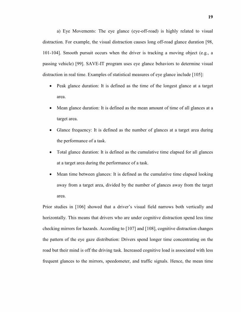
a) Eye Movements: The eye glance (eye-off-road) is highly related to visual
distraction. For example, the visual distraction causes long off-road glance duration [98,
101-104]. Smooth pursuit occurs when the driver is tracking a moving object (e.g., a
passing vehicle) [99]. SAVE-IT program uses eye glance behaviors to determine visual
distraction in real time. Examples of statistical measures of eye glance include [105]:
• Peak glance duration: It is defined as the time of the longest glance at a target
area.
• Mean glance duration: It is defined as the mean amount of time of all glances at a
target area.
• Glance frequency: It is defined as the number of glances at a target area during
the performance of a task.
• Total glance duration: It is defined as the cumulative time elapsed for all glances
at a target area during the performance of a task.
• Mean time between glances: It is defined as the cumulative time elapsed looking
away from a target area, divided by the number of glances away from the target
area.
Prior studies in [106] showed that a driver’s visual field narrows both vertically and
horizontally. This means that drivers who are under cognitive distraction spend less time
checking mirrors for hazards. According to [107] and [108], cognitive distraction changes
the pattern of the eye gaze distribution: Drivers spend longer time concentrating on the
road but their mind is off the driving task. Increased cognitive load is associated with less
frequent glances to the mirrors, speedometer, and traffic signals. Hence, the mean time
20
between glances for distracting driving is longer compared to the value for normal
driving.
b) Head movements: Miyaji et al. [109] found that the standard deviation of the
head movement is suitable for measuring driver distraction. Distraction levels can be
measured by the changes of the head position. It was found that changes of the head
position depend on different face orientations (i.e., frontal, left, right, up and down)
[110].
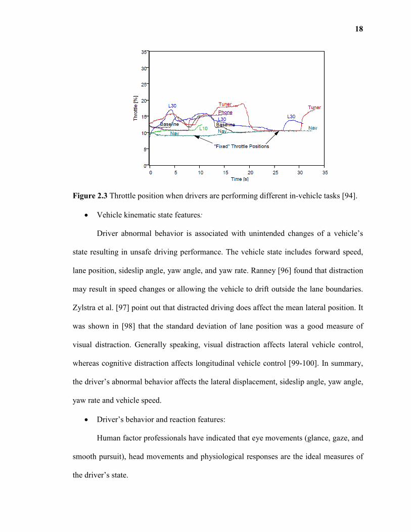
c) Physiological Responses: It was reported in [109] that pupil dilation occurs
when a driver is talking, which results in cognitive distraction. The pupil diameter,
vertical rotation “pitch angle” component and a lateral rotation “yaw angle” component
are shown in Figure 2.4.
Figure 2.4 Pupil diameter and gaze angles [109].
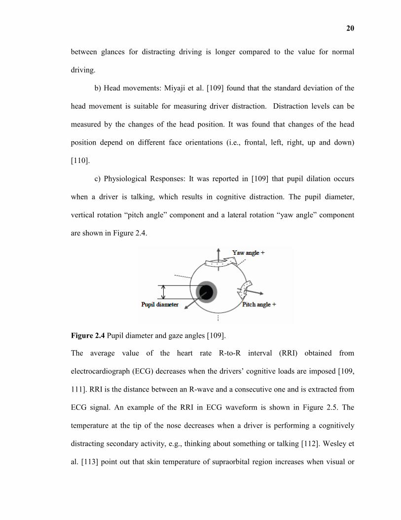
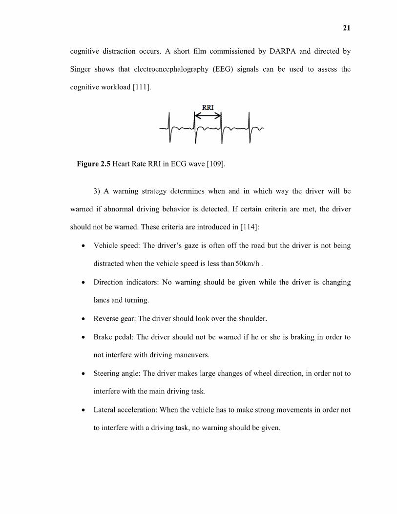
The average value of the heart rate R-to-R interval (RRI) obtained from
electrocardiograph (ECG) decreases when the drivers’ cognitive loads are imposed [109,
111]. RRI is the distance between an R-wave and a consecutive one and is extracted from
ECG signal. An example of the RRI in ECG waveform is shown in Figure 2.5. The
temperature at the tip of the nose decreases when a driver is performing a cognitively
distracting secondary activity, e.g., thinking about something or talking [112]. Wesley et
al. [113] point out that skin temperature of supraorbital region increases when visual or
21
cognitive distraction occurs. A short film commissioned by DARPA and directed by
Singer shows that electroencephalography (EEG) signals can be used to assess the
cognitive workload [111].
Figure 2.5 Heart Rate RRI in ECG wave [109].
3) A warning strategy determines when and in which way the driver will be
warned if abnormal driving behavior is detected. If certain criteria are met, the driver
should not be warned. These criteria are introduced in [114]:
• Vehicle speed: The driver’s gaze is often off the road but the driver is not being
distracted when the vehicle speed is less than50km/h .
• Direction indicators: No warning should be given while the driver is changing
lanes and turning.
• Reverse gear: The driver should look over the shoulder.
• Brake pedal: The driver should not be warned if he or she is braking in order to
not interfere with driving maneuvers.
• Steering angle: The driver makes large changes of wheel direction, in order not to
interfere with the main driving task.
• Lateral acceleration: When the vehicle has to make strong movements in order not
to interfere with a driving task, no warning should be given.
22
On the contrast, the warnings should be triggered while the driver distraction is
detected and a driver is not at one of the above situations [115]. Basically, there are three
main types of warnings:
• Visual warning, e.g., lights, icons, or text warning.
• Auditory warning, e.g., sounds or voice.
• Vibration warning, e.g., seat vibration or steering wheel vibration.
2.5.3 Driver Behavior Classification Algorithms
There have been many research studies on developing algorithms that can effectively
detect a driver’s abnormality in advanced driver assistance systems (e.g., crash warning
systems, lane keeping systems, and etc.). In order to determine whether a driver behavior
is normal or not, the extracted features need to be mapped to a decision. Basically, a
driver’s behavior is considered as being abnormal when a threshold is reached. This can
be viewed as direct matching method. However, abnormal driver behavior can hardly be
represented by a linear model and cannot be classified only by a simple matching
method. Therefore, the machine learning technology is often employed. Different
nonlinear classifiers are designed and tested in the prior research activities:
1) K-nearest neighbor (K-NN):
K-NN is a classification method based on closest training examples in the feature
space. It is the simplest of all machine learning algorithms: an object is classified by a
majority vote of its k nearest neighbors [116]. Sathyanarayana et al. [117] propose a
system for detecting driver distractions using K-Nearest Neighbors (K-NN) classifier
(K=1). The accuracies of distraction detection (classification) using K-NN, principal
23
component analysis (PCA) with K-NN and Linear Discriminate Analysis (LDA) with K-
NN are 77.77%, 94.44%, and 88.30% respectively.
2) Bayesian Networks (BNs):
BN is a probabilistic model that represents a set of random variables. The nodes
in it depict random variables and arrows depict conditional relationship between
variables. There are two main types of BNs: static and dynamic. The former describes the
situations that are not affected by previous states. The latter includes two Static BNs at
successive time steps and the current state of variable depends on the state at the previous
time step. It can modeled as a time-series signals according to a Markov process. BNs
have been used for human behavior modeling, document classification, information
retrieval, image processing, and data fusion. One advantage of BNs is that they provide
an easier form of knowledge representation rather than a complete joint distribution.
Another one is that they can handle situations with missing data. Their effectiveness has
been demonstrated in the application of detecting cognitive distraction [118-119].
3) Decision tree:
A decision tree is a decision support tool that uses a tree-like graph or model of
decisions and their possible consequences. It is commonly used in operations research to
help identify a strategy most likely to reach a goal. Another use is to calculate conditional
probabilities. It has two advantages: simple to understand and interpret, and easy to
combine with other decision techniques. In [120], it is used to estimate the level of
drivers’ cognitive workload from the information of eye glances and driving
performance. A decision tree is used to estimate the driver’s cognitive workload from eye
glances and driving performance [44].
24
4) Support Vector Machines (SVMs):
SVMs original proposed by Vapnik in 1995 are based on statistical learning
theory. In the case of SVMs, a data point is viewed as a p-dimensional vector (a list of p
numbers), and SVMs can find the best hyperplane that represents the largest separation,
or margin, between two classes. SVMs can be used to represent nonlinear relationship
between variables and classifying data [121]. SVMs have been applied to face
recognition, speech recognition, image recognition, and information retrieval. They enjoy
several advantages: they can generate both linear and nonlinear models with the same
efficiency; provide more robust models compared to linear-regression algorithms; and
can extract information from noisy data. Because of these advantages, they are suitable
for measuring the level of cognitive distraction [122-123]. In [124], they successfully
detect cognitive distraction with an accuracy of 81.1% from eye movements and driving
data. There are detailed discussions about Support Vector Machines (SVMs) used to
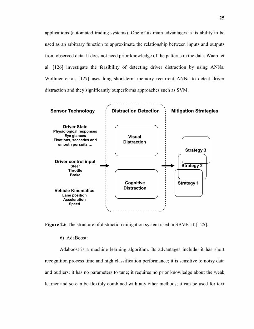
detect distractions in the SAVE-IT project’s final report [125]. The distraction mitigation
system used in the SAVE-IT project is depicted in Figure 2.6.
5) Artificial neural networks (ANNs):
An ANN consists of an interconnected group of artificial neurons. Modern neural
networks are non-linear statistical data modeling tools. They are usually used to model
complex relationships between inputs and outputs or to find patterns in data. It has been
successfully utilized in pattern recognition fields (classification and face identification),
data processing (filtering, clustering and blind source separation); function
approximation, or regression analysis (time series prediction and fitness approximation);
and system identification and control (vehicle control and process control), and financial
25
applications (automated trading systems). One of its main advantages is its ability to be
used as an arbitrary function to approximate the relationship between inputs and outputs
from observed data. It does not need prior knowledge of the patterns in the data. Waard et
al. [126] investigate the feasibility of detecting driver distraction by using ANNs.
Wollmer et al. [127] uses long short-term memory recurrent ANNs to detect driver
distraction and they significantly outperforms approaches such as SVM.
Figure 2.6 The structure of distraction mitigation system used in SAVE-IT [125].
6) AdaBoost:
Adaboost is a machine learning algorithm. Its advantages include: it has short
recognition process time and high classification performance; it is sensitive to noisy data
and outliers; it has no parameters to tune; it requires no prior knowledge about the weak
learner and so can be flexibly combined with any other methods; it can be used for text
Strategy 3
Strategy 2
Sensor Technology Distraction Detection
Visual
Distraction
Cognitive
Distraction
Mitigation Strategies
Vehicle Kinematics Lane position Acceleration
Speed
Driver State Physiological responses
Eye glances Fixations, saccades and
smooth pursuits
Driver control input Steer
Throttle
Brake
Strategy 1
26
categorization, face detection and object detection [128-129]. Miyaji et al. [109]
employed Adaboost to detect driver’s cognitive distraction using physiological features.
7) Hidden Markov Model (HMM):
An HMM is a statistical Markov model in which the system being modeled is
assumed to be a Markov process with hidden states. It consists of a number of states and
transition probabilities and can be considered as the simplest dynamic Bayesian network.
It has been applied in many fields, for example, speech, handwriting, gesture recognition;
machine translation; and gene prediction. It is suitable to recover a data sequence that is
not directly observable and could provide a better performance than conventional
statistical approaches to model human factors and human behaviors. In [130], it was
utilized to construct a framework to deal with the driver distraction detection and driving
maneuver recognition.
2.6 Lateral Control System
The Automated Highway System (AHS) is a type of advanced driver assistance system.
The research on AHS is supported by U.S. Department of Transportation from late 1994.
AHS has been investigated by a number of research groups, such as National Automated
Highway System Consortium in the United States, Intelligent Transport Systems (ITS)
Japan, California PATH in the United States, etc [131-134]. The AHS concept defines a
relationship between vehicles and the highway infrastructure. It uses vehicle and highway
control technologies to shift driving functions from the driver/operator to the vehicle
[51].
The two basic tasks for the AHS are vehicle longitudinal control and vehicle
lateral control. Longitude control includes vehicle speed regulation to maintain adequate
27
spacing between vehicles. This type of control is suitable for preview-based and
anticipatory control. Lateral control mainly refers to automatic vehicle steering to follow
a track reference [52]. This type of control prevents vehicles deviating from the road.
This dissertation focuses on the steering lateral control for the purpose of enhancing
driving safety.
The lateral control strategies can be categorized into two groups: look-ahead and
look-down reference systems. The former measures the lateral displacement from the
lane reference ahead of the vehicle to do the preview-based control. Radar and machine
vision based systems belong to this category and examples of successful projects using
look-ahead reference system include VaMoRs-P, VITA-I and II, Carnegie Mellon
University’s PANS, and California PATH’s stereo-vision based system [133, 135-137].
The latter measures the lateral displacement within or very close to the boundaries of the
vehicle (e.g., straight down from the front bumper of the vehicle). For example, magnetic
markers reference system and electric wire are its examples [54-55,138-139]. Magnetic
markers use different encoding techniques to achieve the preview of road geometry.
Electric wire is used to measure a vehicle’s lateral state via the sensing of a magnetic
field. Compared with the look-ahead reference system, a look-down reference system has
some advantages [58, 79]:
1) It is reliable, yielding accuracy and good performance under any weather or
light condition.
2) Other vehicles will not block the lateral displacement sensing signal.
Some steering control systems based on look-down reference system have been
proposed in the literature [53-56]. More specifically, a general structure of the lateral
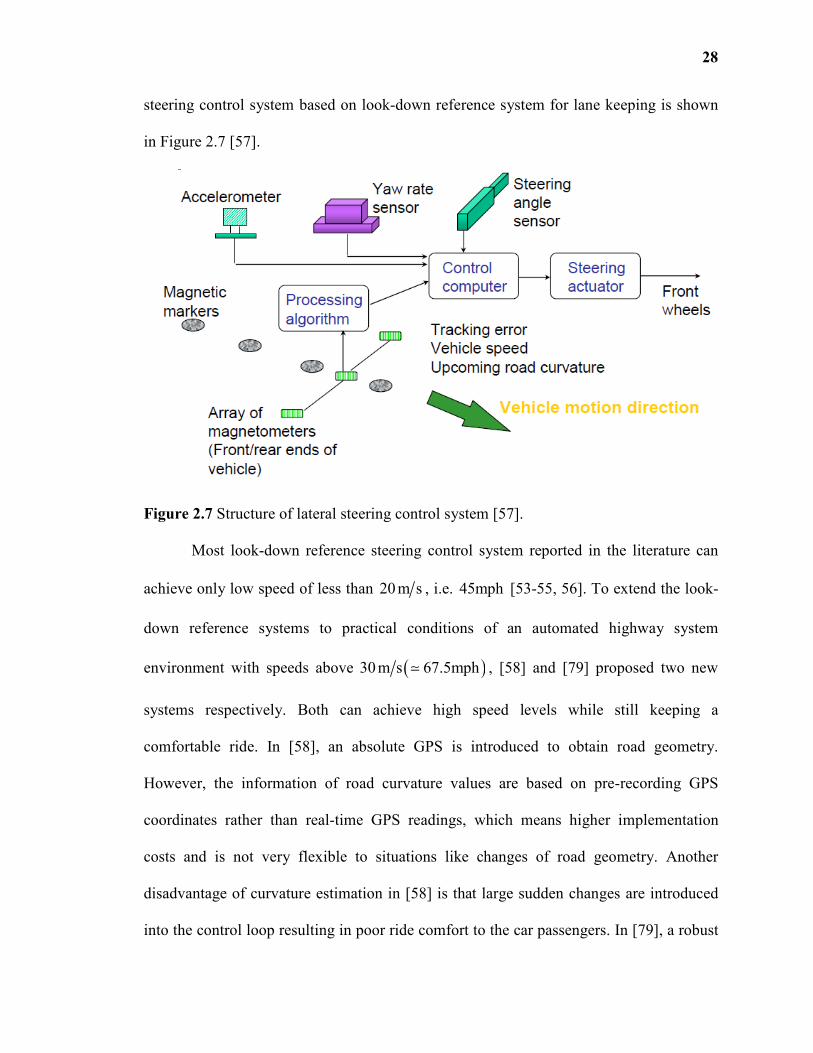
28
steering control system based on look-down reference system for lane keeping is shown
in Figure 2.7 [57].
Figure 2.7 Structure of lateral steering control system [57].
Most look-down reference steering control system reported in the literature can
achieve only low speed of less than 20m s , i.e. 45mph [53-55, 56]. To extend the look-
down reference systems to practical conditions of an automated highway system
environment with speeds above ( )30m s 67.5mph≃ , [58] and [79] proposed two new
systems respectively. Both can achieve high speed levels while still keeping a
comfortable ride. In [58], an absolute GPS is introduced to obtain road geometry.
However, the information of road curvature values are based on pre-recording GPS
coordinates rather than real-time GPS readings, which means higher implementation
costs and is not very flexible to situations like changes of road geometry. Another
disadvantage of curvature estimation in [58] is that large sudden changes are introduced
into the control loop resulting in poor ride comfort to the car passengers. In [79], a robust
29
automatic steering control system is investigated based on the road geometry information
encoded in magnetic markers and lateral displacements from front and rear sensors.
However, this approach utilizes a gyroscope to record the steering angles of the vehicle
and requires a large amount of magnetic markers installed on a highway, which means
higher costs. In addition, the encoding of the road information needs to be implemented
in advance in this system. This is not flexible to changes of road geometry. Moreover,
binary polarity coding technique used in this approach is susceptible to errors.
30
CHAPTER 3
VEHICLE DYNAMICS
This chapter explains fundamental concepts of vehicle dynamics by introducing
single-track model and two-wheel extended nonlinear model which are used in this
research work. The introduced models will help to form the basic idea of a vehicle’s states
and parameters that are related to the driving behaviors and vehicle motions.
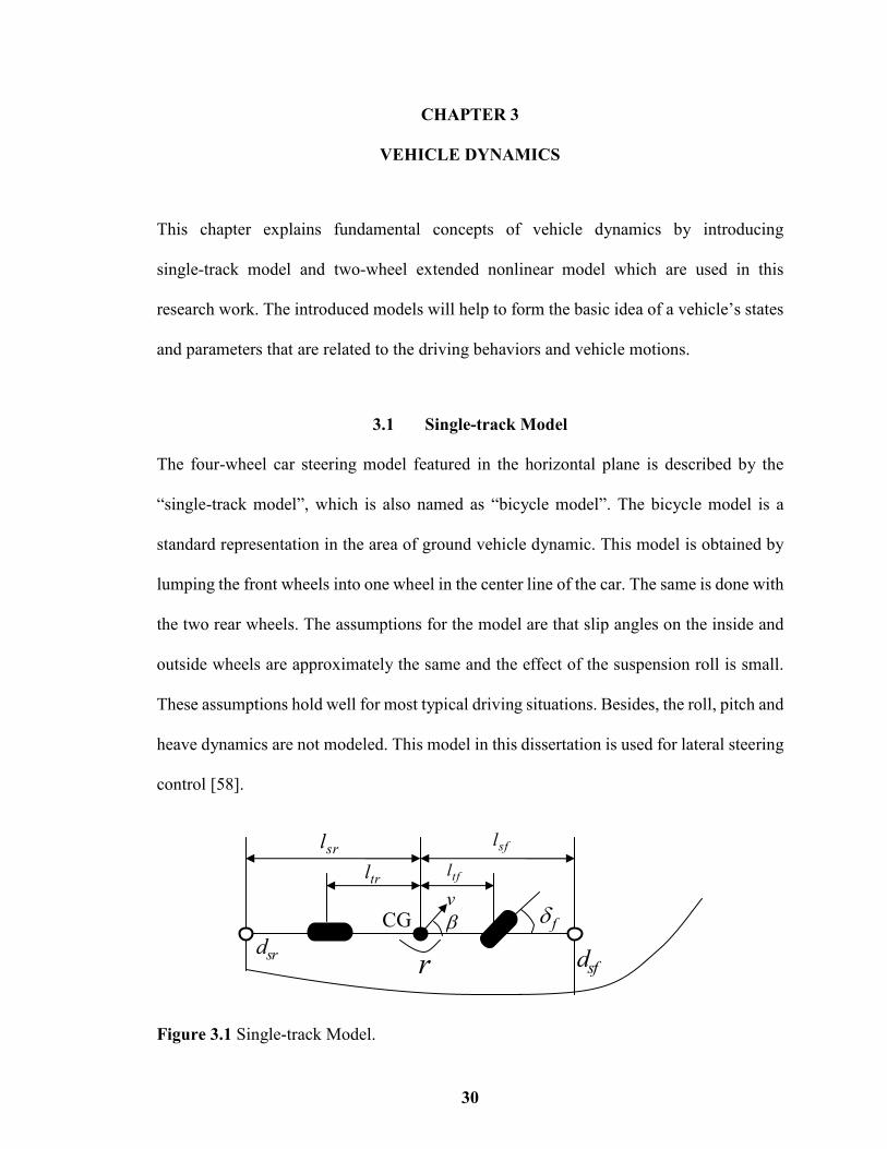
3.1 Single-track Model
The four-wheel car steering model featured in the horizontal plane is described by the
“single-track model”, which is also named as “bicycle model”. The bicycle model is a
standard representation in the area of ground vehicle dynamic. This model is obtained by
lumping the front wheels into one wheel in the center line of the car. The same is done with
the two rear wheels. The assumptions for the model are that slip angles on the inside and
outside wheels are approximately the same and the effect of the suspension roll is small.
These assumptions hold well for most typical driving situations. Besides, the roll, pitch and
heave dynamics are not modeled. This model in this dissertation is used for lateral steering
control [58].
Figure 3.1 Single-track Model.
sfdsrdr
srl sfl
trl tfl
v
β fδCG
31
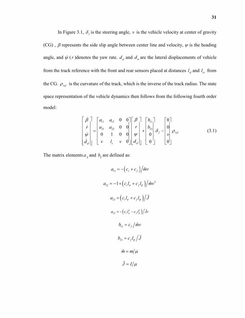
In Figure 3.1, f
δ is the steering angle, v is the vehicle velocity at center of gravity
(CG) , β represents the side slip angle between center line and velocity, ψ is the heading
angle, and ψɺ ( r )denotes the yaw rate. sfd and srd are the lateral displacements of vehicle
from the track reference with the front and rear sensors placed at distances sfl and srl from
the CG. refρ is the curvature of the track, which is the inverse of the track radius. The state
space representation of the vehicle dynamics then follows from the following fourth order
model:
11 12 11
21 22 21
0 0 0
0 0 0
0 1 0 0 0
0 0 0
f ref
sfssf
a a b
ra ar b
v
dv l vd
ββ
δ ρψψ
= + −
ɺ
ɺ
ɺ
ɺ
(3.1)
The matrix elements ija and ijb are defined as:
( )11 r fa c c mv= − + ɶ
( ) 2
12 1 r tr f tfa c l c l mv= − + + ɶ
( )21 r tr f tfa c l c l J= + ɶ
( )2 2
22 r tr f tfa c l c l Jv= − − ɶ
11 fb c mv= ɶ
21 f tfb c l J= ɶ
m m µ=ɶ
J I µ=ɶ
32
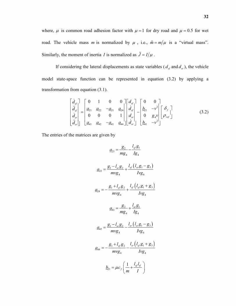
where, µ is common road adhesion factor with 1µ = for dry road and 0.5µ = for wet
road. The vehicle mass m is normalized by µ , i.e., m m µ=ɶ is a “virtual mass”.
Similarly, the moment of inertia I is normalized as J I µ=ɶ .
If considering the lateral displacements as state variables ( sfd and srd ), the vehicle
model state-space function can be represented in equation (3.2) by applying a
transformation from equation (3.1).
2
21 22 21 24 21
4
2
41 42 41 44 41
0 1 0 0 0 0
0 0 0 1 0
sfsf
fsfsf
refsrsr
srsr
dd
da a a a b vd
d g vd
da a a a b vd
δρ
− − = −
− −
ɺ
ɺɺɺ
ɺ
ɺɺɺ
(3.2)
The entries of the matrices are given by
1221
4 4
sfl gga
mg Ig= −
( )1 31 222
4 4
sf srsrl l g gg l g
amvg Ivg
−−= +
( )1 31 2
24
4 4
sf sfsfl l g gg l g
amvg Ivg
++= − +
1241
4 4
srl gga
mg Ig= +
( )1 31 242
4 4
sr srsrl l g gg l g
amvg Ivg
−−= −
( )1 31 2
44
4 4
sr sfsfl l g gg l g
amvg Ivg
++= − −
21
1 sf tf
f
l lb c
m Iµ
= +
33
41
1 sr tf
f
l lb c
m Iµ
= −
where,
( )1 f tf f tfg c l c lµ= −
( )2 f rg c cµ= +
( )2 2
3 r tr f tfg c l c lµ= +
4 sf srg l l= +
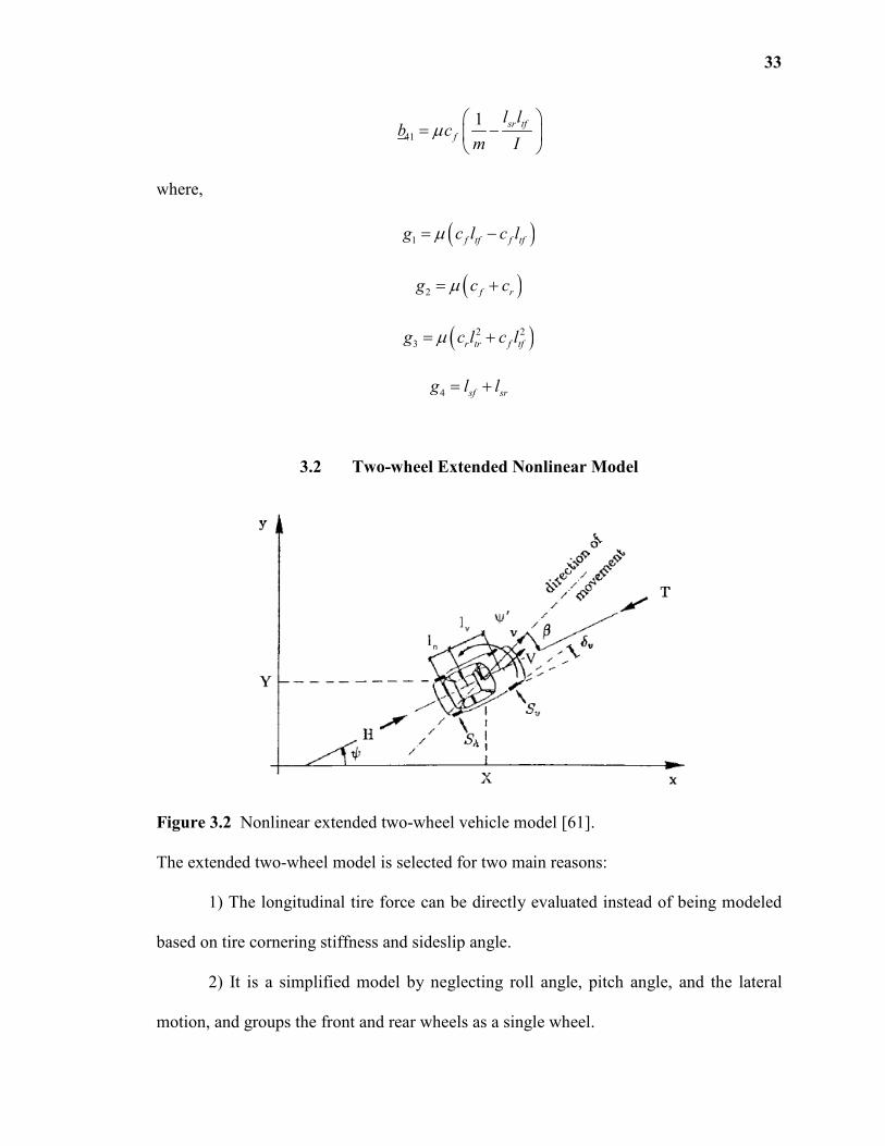
3.2 Two-wheel Extended Nonlinear Model
Figure 3.2 Nonlinear extended two-wheel vehicle model [61].
The extended two-wheel model is selected for two main reasons:
1) The longitudinal tire force can be directly evaluated instead of being modeled
based on tire cornering stiffness and sideslip angle.
2) It is a simplified model by neglecting roll angle, pitch angle, and the lateral
motion, and groups the front and rear wheels as a single wheel.
34
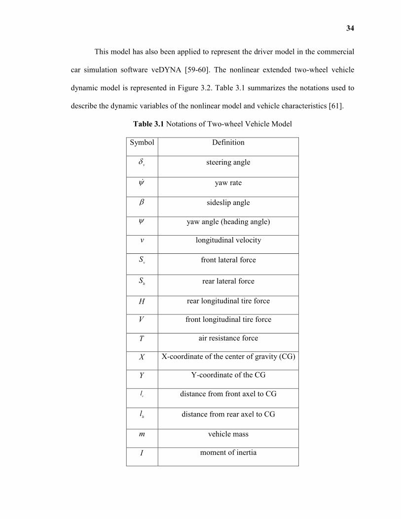
This model has also been applied to represent the driver model in the commercial
car simulation software veDYNA [59-60]. The nonlinear extended two-wheel vehicle
dynamic model is represented in Figure 3.2. Table 3.1 summarizes the notations used to
describe the dynamic variables of the nonlinear model and vehicle characteristics [61].
Table 3.1 Notations of Two-wheel Vehicle Model
Symbol Definition
vδ steering angle
ψɺ yaw rate
β sideslip angle
ψ yaw angle (heading angle)
v longitudinal velocity
vS front lateral force
hS rear lateral force
H rear longitudinal tire force
V front longitudinal tire force
T air resistance force
X X-coordinate of the center of gravity (CG)
Y Y-coordinate of the CG
vl distance from front axel to CG
hl distance from rear axel to CG
m vehicle mass
I moment of inertia
35
In order to derive the state space equations for the simplified vehicle model, the
angles vδ and β are assumed to be small and the front longitudinal force V is neglected.
Then, the nonlinear mode can be described by equation (3.3).
( ) ( )
( )
( )
( )( )
1 13
4 44 4
3
4 2 1
4 2 1
1 11 1
0 0
0
110
0 0cos
0 0sin
h
vhh
T x x S x xx
mx m xm x m x
x
llS x
x wII
T xmm
x x x
x x x
− −+ − −= + − −
−
ɺ (3.3)
The six-dimensional state vector is:
[ ] [ ]' '
1 2 3 4 5 6, , , , , , , , , , .x x x x x x x v X Yβ ψ ψ= = ɺ
The two-dimensional input vector w includes the front lateral force ( )vS x and
longitudinal force H :
[ ] ( )''
1 2 vw w w S x H = = .
The lateral force ( )vS x generated by the front tire is dependent on the steering angle vδ .
More specifically,
( ) 1 3
4
vv v v
lS x x x
xδ
= Γ − +
(3.4)
The rear force ( )hS x and the air resistance ( )T x can be respectively described by
equations (3.5) and (3.6):
( ) 1 3
4
hh h
lS x x x
x
= Γ +
(3.5)
36
( ) 2
42
LwT x c Ax=ℓ
. (3.6)
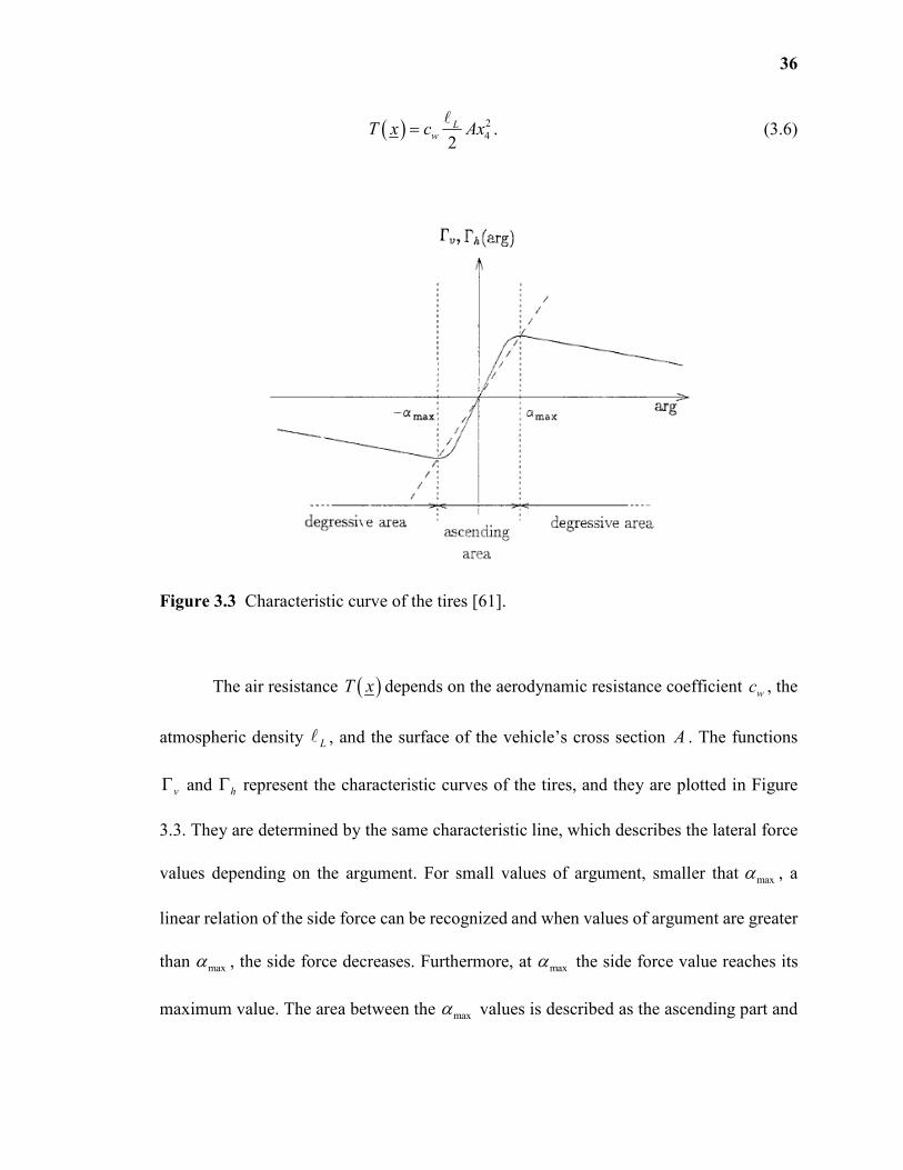
Figure 3.3 Characteristic curve of the tires [61].
The air resistance ( )T x depends on the aerodynamic resistance coefficient wc , the
atmospheric density Lℓ , and the surface of the vehicle’s cross section A . The functions
vΓ and hΓ represent the characteristic curves of the tires, and they are plotted in Figure
3.3. They are determined by the same characteristic line, which describes the lateral force
values depending on the argument. For small values of argument, smaller that maxα , a
linear relation of the side force can be recognized and when values of argument are greater
than maxα , the side force decreases. Furthermore, at maxα the side force value reaches its
maximum value. The area between the maxα values is described as the ascending part and

37
the area outside this area is the descending part of the characteristic line [61]. The
maximum value of maxα is approximated to 6.5 deg [60].
38
CHAPTER 4
LONGITUDINAL TIRE FORCE ESTIMAITON
4.1 Introduction
In this chapter, a driver behavior reconstruction problem is addressed. More specifically,
the task in this study is to estimate the longitudinal tire force which can be transferred to the
corresponding throttle/brake positions under the assumption that the steering angles are
known.
An advanced driver assistance system, utilizing information about the driving
operation behavior (steering angle and throttle/brake positions) and/or vehicle states
(velocity, acceleration, yaw angle, yaw rate, sideslip angle, etc.) can determine potentially
dangerous situations and alert the driver. These critical vehicle parameters can be directly
obtained from the controller area network bus (CAN-bus) in some cars. Although the
parameters can also be collected by installing additional multimodal sensors (such as GPS
receiver, steering angle sensors, throttle/brake pedal position sensors, cameras,
microphones, and etc.), it is inconvenient and costly for the general drivers. Therefore, in
this research, a low cost GPS receiver is used to acquire four types of signals (longitudinal
velocity, yaw angle, lateral and longitudinal positions of the vehicle) instead of using the
high cost vehicle data acquisition equipment. A low cost 1Hz GPS receiver is used as the
vehicle data acquisition equipment. It is obvious that the values of the measurements are
discrete and it is assumed that the steering angles are already known. The aim is to answer
the question on how the longitudinal tire force can be deduced from the partly discrete
knowledge. In this work, a longitudinal force estimation scenario is developed for the
nonlinear extended two-wheel vehicle dynamic model only according to the GPS
39
information. Firstly, two states, i.e. the sideslip angle and the yaw rate are estimated since
they are not available from GPS measurements. Secondly, an optimization scheme is
proposed to estimate the longitudinal tire force. Finally, the estimation results can validate
the proposed methods by comparing to the reference longitudinal tire force command.
For the driver assistance system, the wireless communications technology includes
vehicle data communication from vehicle to vehicle and from vehicle to infrastructure
(e.g., road side station) [63]. The technology enables a number of vehicle safety
applications that mainly focus on improving crash prevention performance and driving
comfort. The Society of Automotive Engineers’ (SAE) common vehicle-to-vehicle safety
message set includes warnings (such as post-crash warning, lane change warning, wrong
way driver warning, etc.) that are transmitted between vehicles to enhance the safety of
driving [64-65]. However, a vehicle-to-vehicle or vehicle-to-station communication
infrastructure is not well established at this point and with the volume of vehicular flow,
communication bandwidth conservation is an important concern. A vehicle-to-station
scenario is considered, in which, the GPS data are transmitted from a vehicle to a road side
station when the vehicle is moving along a certain section of the road. The station
implements vehicle states estimation and the longitudinal tire force estimation tasks, and
reproduces the vehicle’s interpolation motion every second. The station can also determine
the driver behaviors and send the decision back to the vehicle and/or other interested
vehicles that would help other drivers avoid the potential dangerous situation.
Note that the sideslip angle and yaw rate cannot be measured by the GPS receiver.
Since the whole vehicle states are necessary to reconstruct the longitudinal tire force, the
sideslip angle and yaw rate have to be estimated based on the known discrete GPS data
40
points. This is precisely the vehicle state estimation problem. Many methods have been
developed to solve the problem [66]. For example, Extended Kalman Filter (EKF) has been
employed to estimate the dynamic states [67] and most of the EKF methods are designed
based on the four wheel vehicle model. In this research, an estimation methodology for
nonlinear extended two-wheel vehicle model [61] is derived by implementing an Kalman
Filter estimation method. Then, the vehicle states estimation results together with the GPS
signals are further used to calculate the longitudinal tire force. Since the vehicle states
obtained by the GPS receiver and estimated by the Kalman Filter are both discrete, the
procedure to estimate the longitudinal tire force can be viewed as a piecewise
time-independent optimization problem. In the optimization scheme, the optimal
longitudinal tire force is calculated by considering the kinematic constraints.
4.2 Approximated Two-wheel Vehicle Dynamics
The vehicle model used here is the nonlinear two-wheel vehicle model described in
equation (3.3), Section 3.2. Since the tire forces are determined by a characteristic curve
shown in Figure 3.3. The function of vΓ and hΓ defined in equations (3.4) and (3.5) have
to be approximated.
The assumptions adopted are that the angles v
δ and β are small. Besides, the
actual values of 3
4
hl xx
and 3
4
vl xx
are also small because the value of vehicle’s velocity is
large as compared to that of 3hl x and 3vl x . Assume that the arguments of vΓ and hΓ
belong to the ascending area, i.e., 1 3
4
6.5deghv
lx x
xδ− + < and 1 3
4
6.5deghlx xx
+ < . Then,
41
both the functions vΓ and hΓ can be approximated by linear functions, which are
described in the following.
( ) 1 3
4
vv v v
lS x x x
xγ δ
= − +
(4.1)
( ) 1 3
4
hh h
lS x x x
xγ
= +
(4.2)
where the constants vγ and hγ are the slope coefficients for the two linear functions,
respectively. Under the above approximation, the steering angle vδ and the longitudinal tire
force H can be used as the new input vector for the vehicle model. The vehicle model
described in equation (3.3) can be rewritten as
( ) ( )x A x B x u= +ɺ (4.3)
where,
vu
H
δ =
( )
( ) ( )
( )( )
1 3 4 1 3 44 13
4 4
3
1 3 1 3
4 4
2
4
4 2 1
4 2 1
2
1
2
cos
sin
h h v vw L
h h v v v
w L
x l x x x l x xc Ax xx
m mx mx
x
l l l lx x x x
A x I x I x
c Axm
x x x
x x x
γ γ
γ
+ −+ − −
− + + − =
−
−
−
ℓ
ℓ
42
( )
4 1 4
0 0
0
0 1
0 0
0 0
v
v v
mx x m x
l IB x
m
γ
γ
− −
=
4.3 Sideslip Angle and Yaw Rate Estimation
In order to estimate the longitudinal force, it is necessary to measure the values of all the
variables. The GPS receiver is used to measure the velocity, yaw angle, X-position and
Y-position. The sideslip angle β and the yaw rate ψɺ are not available and the vehicle state
observer needs to be designed. The continuous observer used in [61] cannot be used in this
case because the data collected by the GPS is not continuous. In addition, other discrete
EKF methods based on four-wheel model [66-67] are also not suitable for this study.
Therefore, the discrete-time Kalman Filter [68-69] is developed to estimate the sideslip
angle and the yaw rate in this case.
To simplify the estimation problem, a subsystem is considered in which the state
vector is composed of the sideslip angle, the yaw angle, and the yaw rate. It is also
assumed that the fourth variable, vehicle velocity, is constant. This subsystem model can
be simplified to the following time varying nonlinear model from equation (4.3).
1
2
2 2
0 12
0 0 1 0 0
00
w L h v h h v v v
v vv v h h v v
c Av l l x
m mv mv mv mv
x x u
ll l l l
II Iv
y x
γ γ γ γ γ
γγ γ
+ − − − − −
= + − + −
=
ℓ
ɺ (4.4)
where [ ]',vu Hδ= and [ ] [ ]' '
1 2 3, , , ,x x x x β ψ ψ= = ɺ .
43
In order to develop a discrete-time KF, the dynamic model of equation (3.4) has to
be discretized. The discretization is performed by a forward Euler approximation. The step
size is 1T s∆ = , because the receiver updates the data every second. The nonlinear
discrete-time system of the form can be obtained:
( )1 ,k k k
k k k
x f x u
y x n
+ =
= + (4.5)
where kn is the measurement noise vector, which is related to the accuracy of the GPS
receiver. It is supposed to be non-intercorrelated, stationary, white and Gaussian with
known covariance. The covariance of kn is denoted as kR .
The discretized kinematic of the vehicle velocity is
2
1
1
2
kk k w L k
Hv v c Av
m m+ = − +ℓ (4.6)
Then, the force at each time instant k has the form of
( ) 2
1
1
2k k k w L kH m v v c Av+= − + ℓ . (4.7)
There is thus only one input ,v kδ left if replacing kH with the above expression. The
mathematical description of discrete subsystem yields to a linear case,
1 ,k k k k v k
k k k
x A x B
y x n
δ+ = +
= + (4.8)
where,
[ ]' '
1, 2, 3,, , , ,
k k k k k k kx x x x β ψ ψ = = ɺ
44
1
2
2 2
2 0 1
0 1 1
0 1
h v k h h v v
k k k
k
v v h h v v
k
v l l
mv v mv
A
l l l l
I Iv
γ γ γ γ
γ γ
+ + −− − −
=
− + −
'
0v v vk
k
lB
mv I
γ γ = −
In real situation, the measurements are corrupted by noise. Denote
,k k knψψ ψ= +ɶ as the measurements obtained by the GPS. ,knψ is the measurement noise for
the yaw angle. Combining the GPS information and the linear subsystem model of
equation (4.4), the measurement vector ky is defined by:
1. 2 1 ,k k k k v ky a b c dψ ψ ψ δ+ += + + +ɶ ɶ ɶ (4.9)
2,k ky ψ= ɶ (4.10)
3, 1k k ky ψ ψ+= −ɶ ɶ (4.11)
where the coefficients , , ,a b c d are determined by equation (4.8).
( )v v ha I l lγ= − (4.12)
( ) ( )2 2 2h v v k k v v hb l l Iv v l lγ γ= + − − (4.13)
( ) ( )2 2
h v v k k v v hc l l Iv v l lγ γ= − + − − (4.14)
( )v v v v hd l l lγ γ= − − . (4.15)
Under these hypotheses, a discrete Kalman Filter can be applied to the estimation
problem. The Kalman Filter algorithm is recursive and operates in two steps: a prediction
step and an update step. At time step k , { }| 1ˆ |k k k kx E x y y= … is a posteriori estimate of
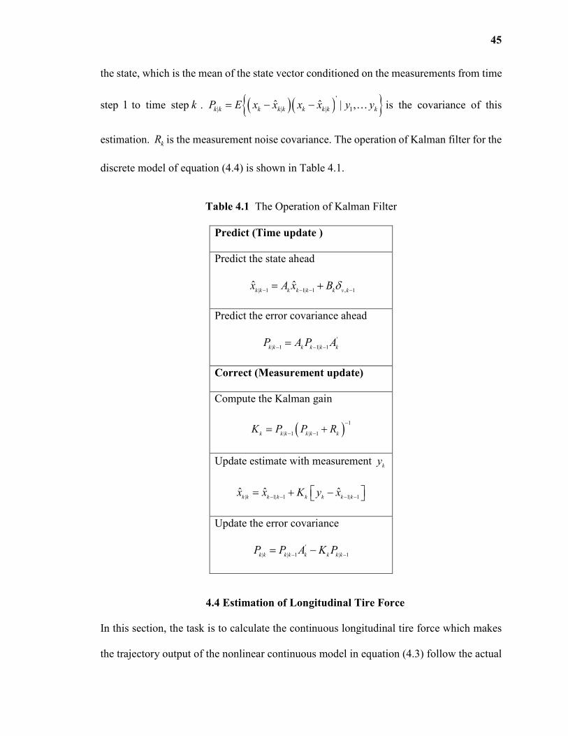
45
the state, which is the mean of the state vector conditioned on the measurements from time
step 1 to time step k . ( )( ){ }'
| | | 1ˆ ˆ | ,k k k k k k k k kP E x x x x y y= − − … is the covariance of this
estimation. kR is the measurement noise covariance. The operation of Kalman filter for the
discrete model of equation (4.4) is shown in Table 4.1.
Table 4.1 The Operation of Kalman Filter
Predict (Time update )
Predict the state ahead
| 1 1| 1 , 1
ˆ ˆk k k k k k v kx A x B δ− − − −= +
Predict the error covariance ahead
'
| 1 1| 1k k k k k kP A P A− − −=
Correct (Measurement update)
Compute the Kalman gain
( ) 1
| 1 | 1k k k k k kK P P R
−
− −= +
Update estimate with measurement ky
| 1| 1 1| 1ˆ ˆ ˆk k k k k k k kx x K y x− − − − = + −
Update the error covariance
'
| | 1 | 1k k k k k k k kP P A K P− −= −
4.4 Estimation of Longitudinal Tire Force
In this section, the task is to calculate the continuous longitudinal tire force which makes
the trajectory output of the nonlinear continuous model in equation (4.3) follow the actual
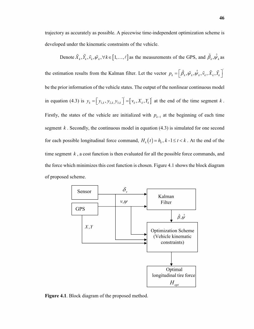
46
trajectory as accurately as possible. A piecewise time-independent optimization scheme is
developed under the kinematic constraints of the vehicle.
Denote [ ], , , , 1, ,k k k kX Y v kψ ∀ ∈ɶ ɶ ɶɶ … ℓ as the measurements of the GPS, and ˆ ˆ,k kβ ψɺ as
the estimation results from the Kalman filter. Let the vector '
ˆ ˆ, , , , ,k k k k k k kp v X Yβ ψ ψ = ɶ ɶɶ ɺ ɶ
be the prior information of the vehicle states. The output of the nonlinear continuous model
in equation (4.3) is [ ]' '
1, 2, , 3,, , ,k k k k k k ky y y y v X Y = = at the end of the time segment k .
Firstly, the states of the vehicle are initialized with 1kp − at the beginning of each time
segment k . Secondly, the continuous model in equation (4.3) is simulated for one second
for each possible longitudinal force command, ( ) , -1k kH t h k t k= ≤ < . At the end of the
time segment k , a cost function is then evaluated for all the possible force commands, and
the force which minimizes this cost function is chosen. Figure 4.1 shows the block diagram
of proposed scheme.
Figure 4.1. Block diagram of the proposed method.
Kalman
Filter
Optimization Scheme
(Vehicle kinematic
constraints)
Sensor
GPS
vδ
,v ψ
,X Y
ˆ ˆ,β ψɺ
Optimal
longitudinal tire force
optH
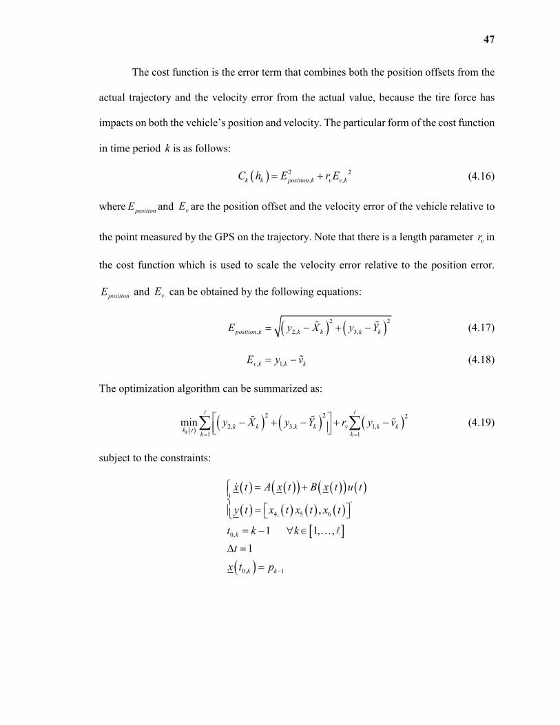
47
The cost function is the error term that combines both the position offsets from the
actual trajectory and the velocity error from the actual value, because the tire force has
impacts on both the vehicle’s position and velocity. The particular form of the cost function
in time period k is as follows:
( ) 2 2
, ,k k position k v v kC h E r E= + (4.16)
where positionE and vE are the position offset and the velocity error of the vehicle relative to
the point measured by the GPS on the trajectory. Note that there is a length parameter vr in
the cost function which is used to scale the velocity error relative to the position error.
positionE and vE can be obtained by the following equations:
( ) ( )2 2
, 2, 3,position k k k k kE y X y Y= − + −ɶ ɶ (4.17)
, 1,v k k kE y v= − ɶ (4.18)
The optimization algorithm can be summarized as:
( )( ) ( ) ( )
2 2 2
2, 3, 1,
1 1
mink
k k k k v k kh t
k k
y X y Y r y v= =
− + − + − ∑ ∑ℓ ℓ
ɶ ɶ ɶ (4.19)
subject to the constraints:
( ) ( )( ) ( )( ) ( )
( ) ( ) ( ) ( )
[ ]
( )
'
4, 5 6
0,
0, 1
,
1 1, ,
1
k
k k
x t A x t B x t u t
y t x t x t x t
t k k
t
x t p −
= +
= = − ∀ ∈
∆ =
=
ɺ
… ℓ
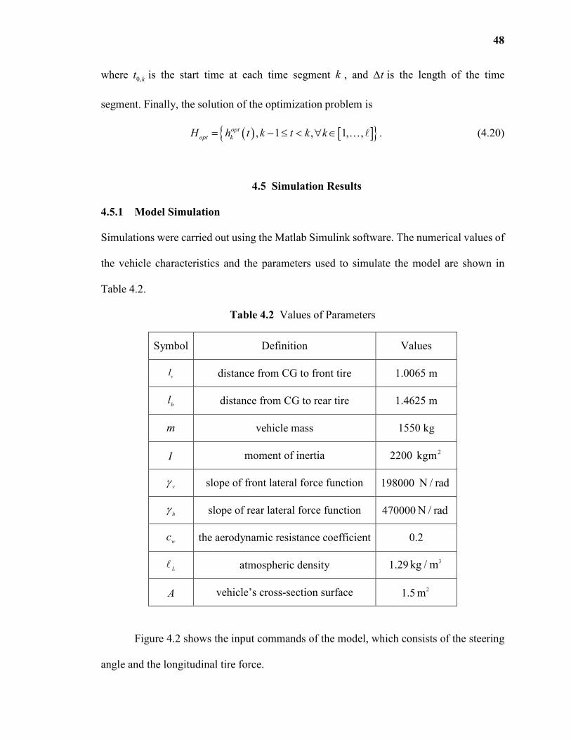
48
where 0,kt is the start time at each time segment k , and t∆ is the length of the time
segment. Finally, the solution of the optimization problem is
( ) [ ]{ }, 1 , 1, ,opt
opt kH h t k t k k= − ≤ < ∀ ∈ … ℓ . (4.20)
4.5 Simulation Results
4.5.1 Model Simulation
Simulations were carried out using the Matlab Simulink software. The numerical values of
the vehicle characteristics and the parameters used to simulate the model are shown in
Table 4.2.
Table 4.2 Values of Parameters
Symbol Definition Values
vl distance from CG to front tire 1.0065 m
hl distance from CG to rear tire 1.4625 m
m vehicle mass 1550 kg
I moment of inertia 2200 2kgm
vγ slope of front lateral force function 198000 N / rad
hγ slope of rear lateral force function 470000 N / rad
wc the aerodynamic resistance coefficient 0.2
Lℓ atmospheric density 1.29
3kg / m
A vehicle’s cross-section surface 1.52m
Figure 4.2 shows the input commands of the model, which consists of the steering
angle and the longitudinal tire force.
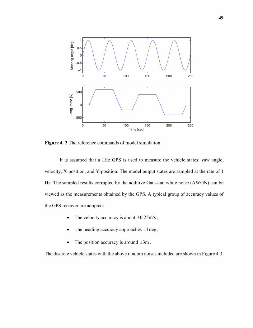
49
0 50 100 150 200 250
−1
−0.5
0
0.5
1
Ste
ering a
ngle
[deg]
0 50 100 150 200 250
−500
0
500
Long. fo
rce [N
]
Time [sec]
Figure 4. 2 The reference commands of model simulation.
It is assumed that a 1Hz GPS is used to measure the vehicle states: yaw angle,
velocity, X-position, and Y-position. The model output states are sampled at the rate of 1
Hz. The sampled results corrupted by the additive Gaussian white noise (AWGN) can be
viewed as the measurements obtained by the GPS. A typical group of accuracy values of
the GPS receiver are adopted:
• The velocity accuracy is about 0.25m/s± ;
• The heading accuracy approaches 1deg± ;
• The position accuracy is around 3m± .
The discrete vehicle states with the above random noises included are shown in Figure 4.3.
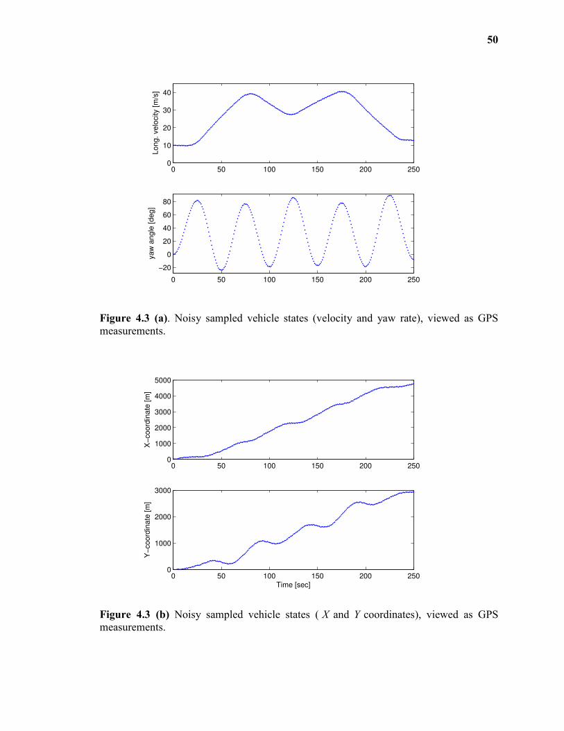
50
0 50 100 150 200 2500
10
20
30
40
Long. velo
city [m
/s]
0 50 100 150 200 250
−20
0
20
40
60
80
yaw
angle
[deg]
Figure 4.3 (a). Noisy sampled vehicle states (velocity and yaw rate), viewed as GPS
measurements.
0 50 100 150 200 2500
1000
2000
3000
4000
5000
X−
coord
inate
[m
]
0 50 100 150 200 2500
1000
2000
3000
Y−
coord
inate
[m
]
Time [sec]
Figure 4.3 (b) Noisy sampled vehicle states ( X and Y coordinates), viewed as GPS
measurements.
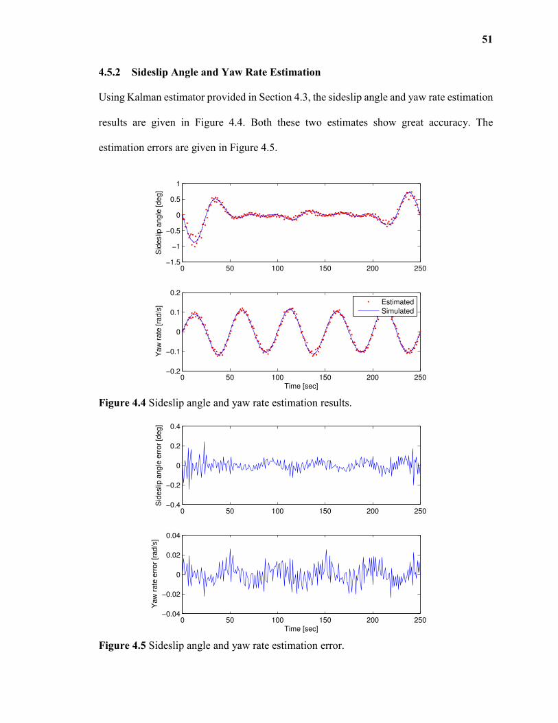
51
4.5.2 Sideslip Angle and Yaw Rate Estimation
Using Kalman estimator provided in Section 4.3, the sideslip angle and yaw rate estimation
results are given in Figure 4.4. Both these two estimates show great accuracy. The
estimation errors are given in Figure 4.5.
0 50 100 150 200 250−1.5
−1
−0.5
0
0.5
1
Sid
eslip
angle
[deg]
0 50 100 150 200 250−0.2
−0.1
0
0.1
0.2
Yaw
rate
[ra
d/s
]
Time [sec]
Estimated
Simulated
Figure 4.4 Sideslip angle and yaw rate estimation results.
0 50 100 150 200 250−0.4
−0.2
0
0.2
0.4
Sid
eslip
angle
err
or
[deg]
0 50 100 150 200 250−0.04
−0.02
0
0.02
0.04
Yaw
rate
err
or
[rad/s
]
Time [sec]
Figure 4.5 Sideslip angle and yaw rate estimation error.
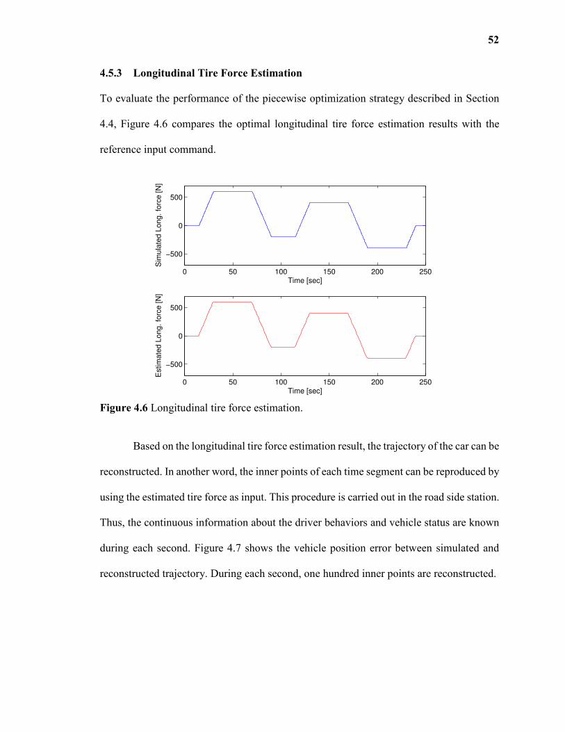
52
4.5.3 Longitudinal Tire Force Estimation
To evaluate the performance of the piecewise optimization strategy described in Section
4.4, Figure 4.6 compares the optimal longitudinal tire force estimation results with the
reference input command.
0 50 100 150 200 250
−500
0
500
Sim
ula
ted L
ong. fo
rce [N
]
Time [sec]
0 50 100 150 200 250
−500
0
500
Estim
ate
d L
ong. fo
rce [N
]
Time [sec]
Figure 4.6 Longitudinal tire force estimation.
Based on the longitudinal tire force estimation result, the trajectory of the car can be
reconstructed. In another word, the inner points of each time segment can be reproduced by
using the estimated tire force as input. This procedure is carried out in the road side station.
Thus, the continuous information about the driver behaviors and vehicle status are known
during each second. Figure 4.7 shows the vehicle position error between simulated and
reconstructed trajectory. During each second, one hundred inner points are reconstructed.
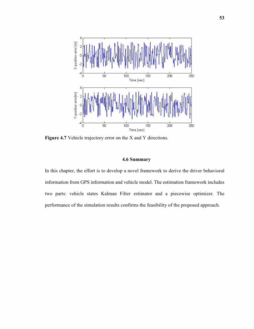
53
Figure 4.7 Vehicle trajectory error on the X and Y directions.
4.6 Summary
In this chapter, the effort is to develop a novel framework to derive the driver behavioral
information from GPS information and vehicle model. The estimation framework includes
two parts: vehicle states Kalman Filter estimator and a piecewise optimizer. The
performance of the simulation results confirms the feasibility of the proposed approach.
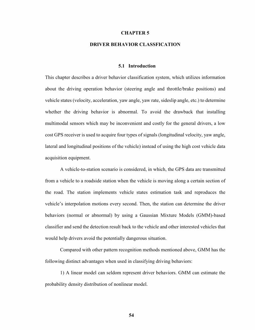
54
CHAPTER 5
DRIVER BEHAVIOR CLASSFICATION
5.1 Introduction
This chapter describes a driver behavior classification system, which utilizes information
about the driving operation behavior (steering angle and throttle/brake positions) and
vehicle states (velocity, acceleration, yaw angle, yaw rate, sideslip angle, etc.) to determine
whether the driving behavior is abnormal. To avoid the drawback that installing
multimodal sensors which may be inconvenient and costly for the general drivers, a low
cost GPS receiver is used to acquire four types of signals (longitudinal velocity, yaw angle,
lateral and longitudinal positions of the vehicle) instead of using the high cost vehicle data
acquisition equipment.
A vehicle-to-station scenario is considered, in which, the GPS data are transmitted
from a vehicle to a roadside station when the vehicle is moving along a certain section of
the road. The station implements vehicle states estimation task and reproduces the
vehicle’s interpolation motions every second. Then, the station can determine the driver
behaviors (normal or abnormal) by using a Gaussian Mixture Models (GMM)-based
classifier and send the detection result back to the vehicle and other interested vehicles that
would help drivers avoid the potentially dangerous situation.
Compared with other pattern recognition methods mentioned above, GMM has the
following distinct advantages when used in classifying driving behaviors:
1) A linear model can seldom represent driver behaviors. GMM can estimate the
probability density distribution of nonlinear model.
55
2) GMM belongs to the class of “unsupervised” classifier which does not require
prior knowledge. Although nobody knows exactly how the driver’s error impairs driving
performance, GMM method may be able to extract the features of this relationship.
3) GMM method produces more robust performance than traditional learning
methods
GMM has been used to analyze the driving behavior in recent research. For
example, [140] used GMM method to detect distracted driving based on in-vehicle
CAN-bus data. A GMM framework was developed to model the driving behaviors with
driving signals (e.g., following distance, vehicle speed) and model pedal operation with
features extracted from raw pedal operation signals [141]. Authors modeled driving
behavior employing GMM based on driving signals such as brake and accelerator pedal
pressure, engine RPM, vehicle speed and steering wheel angle in [142]. In the above
research, the critical driving information can be obtained through different methods. For
instance, driving information can be directly obtained from the CAN-bus in some cars
[140]. The CAN-bus signal contains real-time vehicle information in the form of messages
integrating many modules. Usually, the open connector of the CAN-bus is On-Board
Diagnostics (OBD-II). However, the CAN-bus signal is not available on the OBD-II
connector for all cars. Furthermore, the database used to decode the CAN-bus signal may
not be available to the general public or the cost for the database and data acquisition
software maybe prohibitive. In addition, the driving information can also be collected by
installing additional multimodal sensors, such as gyroscope, steering angle sensors,
throttle/brake pedal position sensors, cameras, microphones, and other sensors [141-142].
It is inconvenient and costly for the general drivers to install these devices. In order to
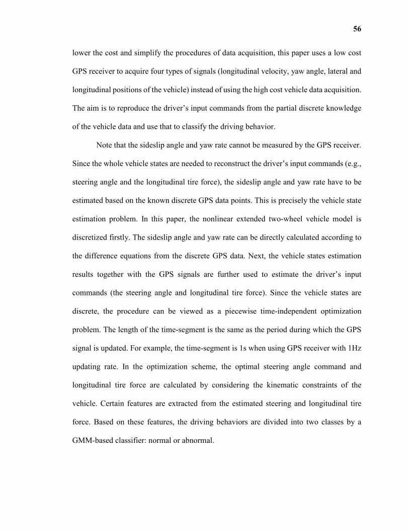
56
lower the cost and simplify the procedures of data acquisition, this paper uses a low cost
GPS receiver to acquire four types of signals (longitudinal velocity, yaw angle, lateral and
longitudinal positions of the vehicle) instead of using the high cost vehicle data acquisition.
The aim is to reproduce the driver’s input commands from the partial discrete knowledge
of the vehicle data and use that to classify the driving behavior.
Note that the sideslip angle and yaw rate cannot be measured by the GPS receiver.
Since the whole vehicle states are needed to reconstruct the driver’s input commands (e.g.,
steering angle and the longitudinal tire force), the sideslip angle and yaw rate have to be
estimated based on the known discrete GPS data points. This is precisely the vehicle state
estimation problem. In this paper, the nonlinear extended two-wheel vehicle model is
discretized firstly. The sideslip angle and yaw rate can be directly calculated according to
the difference equations from the discrete GPS data. Next, the vehicle states estimation
results together with the GPS signals are further used to estimate the driver’s input
commands (the steering angle and longitudinal tire force). Since the vehicle states are
discrete, the procedure can be viewed as a piecewise time-independent optimization
problem. The length of the time-segment is the same as the period during which the GPS
signal is updated. For example, the time-segment is 1s when using GPS receiver with 1Hz
updating rate. In the optimization scheme, the optimal steering angle command and
longitudinal tire force are calculated by considering the kinematic constraints of the
vehicle. Certain features are extracted from the estimated steering and longitudinal tire
force. Based on these features, the driving behaviors are divided into two classes by a
GMM-based classifier: normal or abnormal.
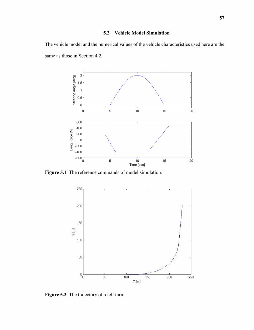
57
5.2 Vehicle Model Simulation
The vehicle model and the numerical values of the vehicle characteristics used here are the
same as those in Section 4.2.
0 5 10 15 20
0
0.5
1
1.5
2S
teering a
ngle
[deg]
0 5 10 15 20−600
−400
−200
0
200
400
600
Time [sec]
Long. fo
rce [N
]
Figure 5.1 The reference commands of model simulation.
Figure 5.2 The trajectory of a left turn.
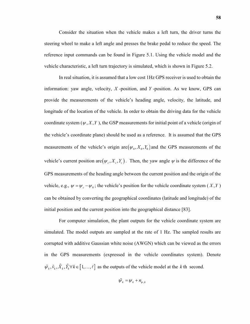
58
Consider the situation when the vehicle makes a left turn, the driver turns the
steering wheel to make a left angle and presses the brake pedal to reduce the speed. The
reference input commands can be found in Figure 5.1. Using the vehicle model and the
vehicle characteristic, a left turn trajectory is simulated, which is shown in Figure 5.2.
In real situation, it is assumed that a low cost 1Hz GPS receiver is used to obtain the
information: yaw angle, velocity, X -position, and Y -position. As we know, GPS can
provide the measurements of the vehicle’s heading angle, velocity, the latitude, and
longitude of the location of the vehicle. In order to obtain the driving data for the vehicle
coordinate system ( , ,X Yψ ), the GSP measurements for initial point of a vehicle (origin of
the vehicle’s coordinate plane) should be used as a reference. It is assumed that the GPS
measurements of the vehicle’s origin are ( )0 0 0, ,X Yψ and the GPS measurements of the
vehicle’s current position are ( ), ,c c cX Yψ . Then, the yaw angle ψ is the difference of the
GPS measurements of the heading angle between the current position and the origin of the
vehicle, e.g., 0cψ ψ ψ= − ; the vehicle’s position for the vehicle coordinate system ( ,X Y )
can be obtained by converting the geographical coordinates (latitude and longitude) of the
initial position and the current position into the geographical distance [83].
For computer simulation, the plant outputs for the vehicle coordinate system are
simulated. The model outputs are sampled at the rate of 1 Hz. The sampled results are
corrupted with additive Gaussian white noise (AWGN) which can be viewed as the errors
in the GPS measurements (expressed in the vehicle coordinates system). Denote
[ ], , , 1, ,k k k kv X Y kψ ∀ ∈ɶ ɶɶ ɶ … ℓ as the outputs of the vehicle model at the thk second.
,k k knψψ ψ= +ɶ
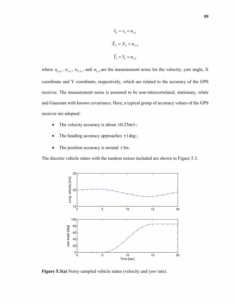
59
,k k v kv v n= +ɶ
,k k X kX X n= +ɶ
,k k Y kY Y n= +ɶ
where ,knψ , ,v kn , ,X kn , and ,Y kn are the measurement noise for the velocity, yaw angle, X
coordinate and Y coordinate, respectively, which are related to the accuracy of the GPS
receiver. The measurement noise is assumed to be non-intercorrelated, stationary, white
and Gaussian with known covariance. Here, a typical group of accuracy values of the GPS
receiver are adopted:
• The velocity accuracy is about 0.25m/s± ;
• The heading accuracy approaches 1deg± ;
• The position accuracy is around 3m± .
The discrete vehicle states with the random noises included are shown in Figure 5.3.
0 5 10 15 2015
20
25
Long. velo
city [m
/s]
0 5 10 15 200
20
40
60
80
100
Time [sec]
yaw
angle
[deg]
Figure 5.3(a) Noisy sampled vehicle states (velocity and yaw rate).
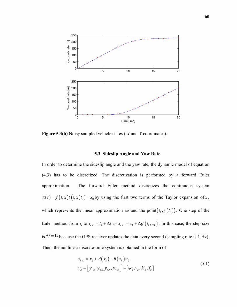
60
0 5 10 15 200
50
100
150
200
250
X−
coord
inate
[m
]
0 5 10 15 200
50
100
150
200
250
Time [sec]
Y−
coord
inate
[m
]
Figure 5.3(b) Noisy sampled vehicle states ( X and Y coordinates).
5.3 Sideslip Angle and Yaw Rate
In order to determine the sideslip angle and the yaw rate, the dynamic model of equation
(4.3) has to be discretized. The discretization is performed by a forward Euler
approximation. The forward Euler method discretizes the continuous system
( ) ( )( ) ( )0 0, ,x t f t x t x t x= =ɺ by using the first two terms of the Taylor expansion of x ,
which represents the linear approximation around the point ( )( )0 0,t y t . One step of the
Euler method from kt to 1k kt t t+ = + ∆ is ( )1 ,k k k kx x tf t x+ = + ∆ . In this case, the step size
is 1t s∆ = because the GPS receiver updates the data every second (sampling rate is 1 Hz).
Then, the nonlinear discrete-time system is obtained in the form of
( ) ( )
[ ]1
' '
1, 2, , 3, 4,, , , , ,
k k k k k
k k k k k k k k k
x x A x B x u
y y y y y v X Yψ
+ = + +
= = (5.1)
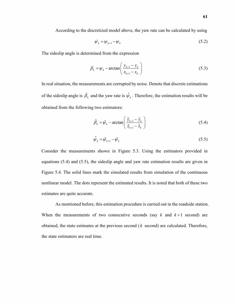
61
According to the discretized model above, the yaw rate can be calculated by using
1k k kψ ψ ψ+= −ɺ (5.2)
The sideslip angle is determined from the expression
1
1
arctan k kk k
k k
y y
x xβ ψ +
+
−= − −
(5.3)
In real situation, the measurements are corrupted by noise. Denote that discrete estimations
of the sideslip angle is ˆkβ and the yaw rate is ˆkψɺ . Therefore, the estimation results will be
obtained from the following two estimators:
1
1
ˆ arctan k kk k
k k
y y
x xβ ψ +
+
−= − −
ɶ ɶɶ
ɶ ɶ (5.4)
1ˆ
k k kψ ψ ψ+= −ɺ ɶ ɶ (5.5)
Consider the measurements shown in Figure 5.3. Using the estimators provided in
equations (5.4) and (5.5), the sideslip angle and yaw rate estimation results are given in
Figure 5.4. The solid lines mark the simulated results from simulation of the continuous
nonlinear model. The dots represent the estimated results. It is noted that both of these two
estimates are quite accurate.
As mentioned before, this estimation procedure is carried out in the roadside station.
When the measurements of two consecutive seconds (say k and 1k + second) are
obtained, the state estimates at the previous second ( k second) are calculated. Therefore,
the state estimators are real time.

62
0 5 10 15 20
−1
−0.8
−0.6
−0.4
−0.2
0
0.2
Time [sec]
Slip
sid
e a
ngle
[deg]
0 5 10 15 20
0
5
10
15
Time [sec]
Yaw
rate
[deg/s
]
Fig 5.4 Sideslip angle and yaw rate estimation.
5.4 Piecewise Optimization Scheme
In this section, the task is to estimate the continuous driver’s input commands which
include steering angle and longitudinal tire force. The goal is to find an optimal solution of
input commands which makes the trajectory output follows the simulated trajectory as
accurately as possible. These are the kinematic constraints of the vehicle. A real time
piecewise optimization scheme under such constraints is developed to solve this estimation
problem.
At the end of the time segment k , [ ], , , , 1, ,k k k kX Y v kψ ∀ ∈ɶ ɶ ɶɶ … ℓ are the
measurements of the GPS receiver, and ˆ ˆ,k kβ ψɺ as the estimation results. Let the vector
'ˆ ˆ, , , , ,k k k k k k kp v X Yβ ψ ψ =
ɶ ɶɶ ɺ ɶ be the prior information of the vehicle states. At the end of the
time segment ,k the output of the discrete model in equation (5.1) is
63
[ ]' '
1, 2, , 3, 4,, , , , ,k k k k k k k k ky y y y y v X Yψ = = . Firstly, the states of the vehicle are initialized
with 1kp − at the beginning of each time segment k . Secondly, the continuous model in
equation (4.3) is simulated for one second for each possible steering angle command
( ), , , -1v k v kt k t kδ∆ = ≤ < and longitudinal force command, ( ) , -1k kH t h k t k= ≤ < . At the
end of the time segment k , a cost function is then evaluated for all of the possible input
commands, and the input commands that minimize this cost function are chosen.
The cost function is the error term that combines both the position offsets from the
actual trajectory and the velocity error from the actual value. The particular form of the
cost function in time period k is as follows:
( ) ( )( ) 2 2
, , ,,k v k k position k v v kC t H t E r E∆ = + (5.6)
where positionE and vE are the position offset and the velocity error of the vehicle relative to
the data point k measured by the GPS receiver on the trajectory. Note that there is a length
parameter vr in the cost function which is used to scale the velocity error relative to the
position error. positionE and vE can be obtained by the following equations:
( ) ( )2 2
, 3, 4,position k k k k kE y X y Y= − + −ɶ ɶ (5.7)
, 2,v k k kE y v= − ɶ (5.8)
The optimization algorithm can be summarized as:
( ) ( )( ) ( ) ( )
,
2 2 2
3, 4, 2,,
1 1
minv k k
k k k k v k kt H t
k k
y X y Y r y v∆
= =
− + − + − ∑ ∑ℓ ℓ
ɶ ɶ ɶ (5.9)
subject to the constraints:
64
( ) ( )( ) ( )( ) ( )
( ) ( ) ( ) ( ) ( )
[ ]
( )
'
2 4 5 6
0,
0, 1
, , ,
1 1, ,
1
k
k k
x t A x t B x t u t
y t x t x t x t x t
t k k
t
x t p −
= +
=
= − ∀ ∈
∆ =
=
ɺ
… ℓ
where 0,kt is the start time at each time segment k , and t∆ is the length of the time
segment. Finally, the solution of the optimization problem is
( ) [ ]{ }, , 1 , 1, ,opt opt
v v k t k t k kδ = ∆ − ≤ < ∀ ∈ … ℓ (5.10)
( ) [ ]{ }, 1 , 1, ,opt opt
kH H t k t k k= − ≤ < ∀ ∈ … ℓ . (5.11)
The global search method is employed to solve the above optimization problem. In
order to simply the searching procedure, the search range can be determined using discrete
kinematics of the vehicle in equation (5.1). The longitudinal force at each time instant k
has the approximate form of
( ) 2
1
1ˆ2
k k k w L kH m v v c Av+= − +ɶ ɶ ɶℓ . (5.12)
The steering angle’s approximation at each time instant k can be obtained by the
expression
, 2 1ˆ ˆv k k k k ka b c dδ ψ ψ ψ β+ += + + +ɶ ɶ ɶ (5.13)
where the coefficients , , ,a b c d are
v v
Ia
lγ= ,
2 2 2h v v k
k v v
l l Ivb
v l
γγ
+ −=
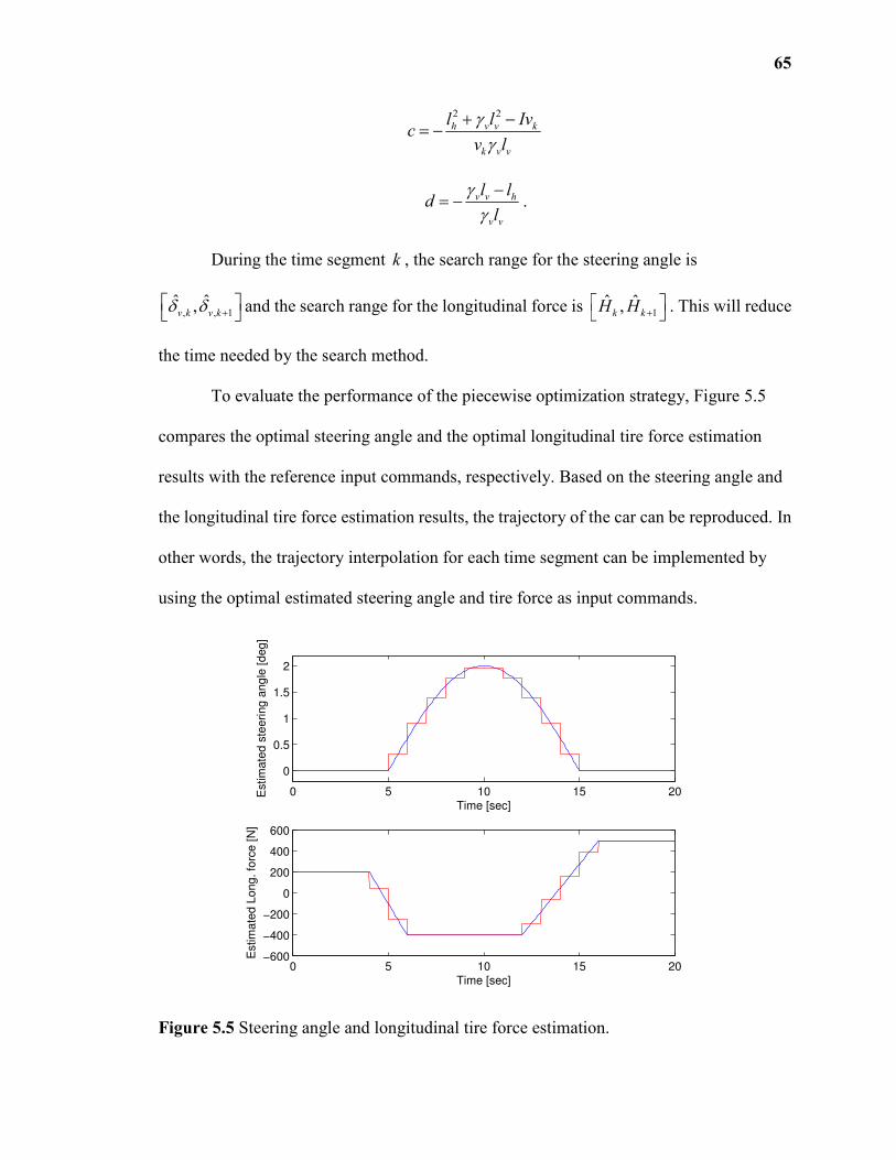
65
2 2
h v v k
k v v
l l Ivc
v l
γγ
+ −= −
v v h
v v
l ld
l
γγ−
= − .
During the time segment k , the search range for the steering angle is
, , 1ˆ ˆ,v k v kδ δ +
and the search range for the longitudinal force is 1
ˆ ˆ,k kH H + . This will reduce
the time needed by the search method.
To evaluate the performance of the piecewise optimization strategy, Figure 5.5
compares the optimal steering angle and the optimal longitudinal tire force estimation
results with the reference input commands, respectively. Based on the steering angle and
the longitudinal tire force estimation results, the trajectory of the car can be reproduced. In
other words, the trajectory interpolation for each time segment can be implemented by
using the optimal estimated steering angle and tire force as input commands.
0 5 10 15 20
0
0.5
1
1.5
2
Time [sec]
Estim
ate
d s
teering a
ngle
[deg]
0 5 10 15 20−600
−400
−200
0
200
400
600
Time [sec]
Estim
ate
d L
ong. fo
rce [N
]
Figure 5.5 Steering angle and longitudinal tire force estimation.
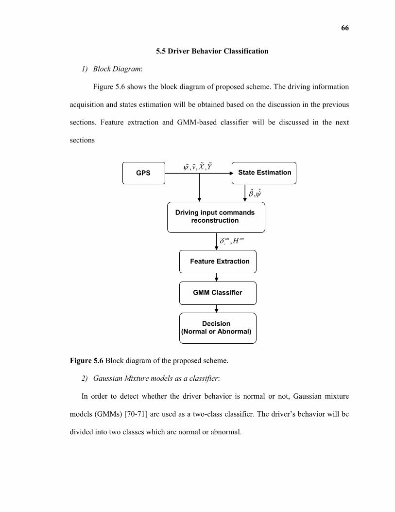
66
5.5 Driver Behavior Classification
1) Block Diagram:
Figure 5.6 shows the block diagram of proposed scheme. The driving information
acquisition and states estimation will be obtained based on the discussion in the previous
sections. Feature extraction and GMM-based classifier will be discussed in the next
sections
Figure 5.6 Block diagram of the proposed scheme.
2) Gaussian Mixture models as a classifier:
In order to detect whether the driver behavior is normal or not, Gaussian mixture
models (GMMs) [70-71] are used as a two-class classifier. The driver’s behavior will be
divided into two classes which are normal or abnormal.
State Estimation
Feature Extraction
Decision (Normal or Abnormal)
Driving input commands reconstruction
GPS , , ,v X Yψ ɶ ɶɶ ɶ
ˆ ˆ,β ψɺ
,opt opt
vHδ
GMM Classifier
67
Gaussian mixture model is a probabilistic model for probability density function
(pdf) estimation using a set of multiple Gaussian distributions. GMM have been a powerful
nonlinear classification tools in many applications of pattern recognition [72-73],
particularly in speech and face recognition. Gaussian mixture models are suitable for
classification of driver behaviors. First, a linear model can seldom represent driver
behaviors. GMM can estimate the probability density distribution of nonlinear model.
Second, GMM belongs to the “unsupervised” classifier category which does not require
prior knowledge before training. Third, the GMM method produces more robust
performance than traditional learning methods (e.g., logistic regression, multi-layer
perceptron). The GMM method may have computational difficulty if the volume of
training data becomes great. However, the GMM method is a robust approach to classify
the driver behavior.
GMM non-linear pattern classifier works by estimating the underlying probability
density functions (pdf’s) of the observations. In the GMM classifier, the conditional-pdf of
the observation vector with respect to the different classes is modeled as a linear
combination of multivariate Gaussian pdf’s. Each of them has the following form:
( )( )
( ) ( )1
22
1 1exp
22
T
dp
π
− = − − Σ − Σ
x x µ x µ (5.14)
where x is a d-component feature vector, µ is the d-component vector containing the mean
of each feature, Σ is the d-by-d covariance matrix, and Σ is its determinant. It is noted that
each multivariate Gaussian pdf can be completely defined if [ ],θ = Σµ is known.

68
In this case, each class (normal or abnormal) is modeled as a GMM based on its
own features. The feature vector is denoted as tx . The assumptions made to build a GMM
are the following [74]:
• The samples come from a known number c ( 2c = ) of classes. The two classes are
denoted as 0C (abnormal) and 1C (normal).
• The priori probabilities ( )iP C for each class iC are known (They are taken to be
all equal to 1 1
2c= ).
• The forms of the class-conditional probability densities
( )| , , 1, , 1,2i ip C i cθ = =x … are known for all classes. It is assumed that they are a
sum of K multivariate Gaussian probability density functions.
• The unknowns are the values of the parameter vectors 1,2iθ = (for each class, the
mean vector and covariance matrix).
Assuming that the probability density function ( )|t ip Cx is a mixture of
K multivariate Gaussian distributions:
( ) ( ) ( )1
| | | ,K
t i i t i
l
p C P l C p l C=
=∑x x (5.15)
where ( ) ( ), ,| , ,t i l i l ip l C N=x µ Σ is the probability of tx being produced by the Gaussian
distribution of index l in class i . ( )| iP l C is the prior probability of having a Gaussian
distribution l for class i . There are two phases for this classification problem: GMM
training and the classification test.
69
In the training phase, the aim is to estimate the parameters of the GMMs for the two
classes: ( ){ }, ,| , , , 1,i i l i l iP l C l KΘ = =µ Σ … with 1,2i = , 1l K= … . An optimization
algorithm called Expectation Maximization (EM) [75] is used to estimate all the
parameters.
The progress of EM algorithm: there are m observations of the features for each
class iC : 1 2, , ,i i i iC C C C
m = X x x x… . Assuming that the observations are independent and
identically distributed, the likelihood that the entire set of observations has been produced
by class iC is:
( ) ( )1
| , |m
i i t i
t
p C p C=
Θ =∏X x . (5.16)
Using the above likelihood function, EM algorithm gives the maximum likelihood
estimates of all the parameters ( ),ˆ argmax log | ,ML i i ip CΘ = ΘX . Since it is hard to directly
maximize the log-likelihood function, EM algorithm maximizes the lower-bound of
log-likelihood function ( ),F q Θ . It has been proved that maximizing the lower-bound is
equivalent to maximizing the expected log-likelihood [84]. EM algorithm is consisted of
two steps: E-step and M-step:
E-step: ( ) ( )( )1
argmax ,t t
q
q F q+ = Θ
M-step: ( ) ( )( )1 1
argmax ,t t
F q+ +
ΘΘ = Θ
Making a first guess on the values of the iΘ and compute E-step and M-step. And the
algorithm converges to a local optimum after conducting iterations. Note that the training
70
set provided to the GMM has to be well thought out in order for the model to be general
enough and avoid the common problem of over-fitting the training data.
In the classification phase, the classification tests using the trained GMMs is
performed. According to the Bayesian rule, a feature vector tx is said to belong to class i
if it maximizes
( ) ( ) ( )( )
||
t i i
i t
t
p C p Cp C
p=
xx
x. (5.17)
In the case it is assumed that the two classes occur with the same probability,
( ) ( )0 1 0.5p C p C= = . It is actually only concerned with maximizing ( )|t ip Cx .
The decision rule for the two-class classifier is:
• tx belongs to the abnormal case if ( ) ( )0 1| |t tp C p C>x x ;
• Otherwise, tx belongs to the normal case.
5.6 Feature Extraction
Since the estimated steering angle and longitudinal tire force are both continuous segment
signals, root mean square (RMS) statistical method is suitable to reflect the driver’s input
activities [85-86]. For example, RMS of the steering angle can reflect the driver’s steering
maneuvers; RMS of the longitudinal tire force can reflect the throttle and brake pedal
operation.
RMS is a second order statistical measure of the magnitude of a continuously
varying function (or waveform). The RMS formula of a continuous function ( )f t defined
over the time interval 1 2T t T≤ ≤ has the following form [87]:
71
( )2
1
2
2 1
1 T
rmsT
f f t dtT T
= − ∫ (5.18)
In this study, the feature vector provided to the GMM-based classifier consists of
the RMS of the reconstructed steering angle and longitudinal tire force.
,opt opt
t Hδ = x (5.19)
5.7 Simulation Results
The performance of abnormal driver behavior detection is verified by simulating the
vehicle model for a left turn (described in section 5.2).
1) Simulating abnormal driving behavior:
Abnormal driving behaviors usually occur when the driving patterns the drivers
make are not smooth, e.g., the sharp movement of the steering wheel [77]. In the UMTRI
research in the SAVE-IT project, it was found that when drivers were performing an
in-vehicle task, they controlled their speed by intermittently adjusting the throttle [78].
According to the above facts and experiments, some assumptions are made to simulate the
abnormal driving patterns for training set:
• Large variations of the reference steering angle and the longitudinal tire force
within a short period of time may reflect abnormal driving behaviors. The form of
such large variations is modeled as AWGN.
• It is assumed that the driving behavior can be viewed as an abnormal case when:
,
,
20%v
v
error
ref
A
A
δ
δ
> or ,
,
20%H error
H ref
A
A> ,
72
where , ,,v ref H refA Aδ are the RMS amplitude of the reference steering angle and the
reference longitudinal tire force, respectively. , ,,v error H errorA Aδ are the RMS
amplitude of the variations between the actual and the reference values of the
steering angle and the longitudinal tire force, respectively. The values of ,v errorAδ
and ,H errorA are generated using AWGN method.
2) GMM training:
The probability density function ( ) ( )| , 1, 2t ip C i =x is modeled by using four
mixtures of Gaussian distribution ( )4K = . The number of training data for both normal
driving and abnormal driving are 50n aM M= = . EM algorithm is used to train the two
GMMs. Experiments demonstrated that the EM method had an acceptable computational
load with this volume of training data.
3) Testing phase:
Since the goal is detecting the abnormal driving behaviors, only classification
performance for the abnormal cases is needed to test. The number of testing data for
abnormal driving is 25aN = . Fifty independent simulations and tests were implemented.
4) Detection Results:
Table 5.1 summarizes the classification results. The average accuracy of the
abnormal driving behavior detection is 87.2%, which means that the average miss
detection rate is approximately 12.8%. The reason for the miss detection is that the GPS
data is sparse and somewhat inaccurate. If the GPS with a higher update rate is adopted, a
more accurate detection result will be achieved.
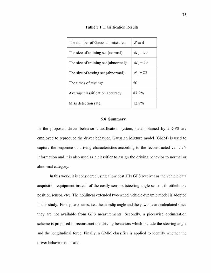
73
Table 5.1 Classification Results
The number of Gaussian mixtures: 4K =
The size of training set (normal): 50nM =
The size of training set (abnormal): 50aM =
The size of testing set (abnormal): 25aN =
The times of testing: 50
Average classification accuracy: 87.2%
Miss detection rate: 12.8%
5.8 Summary
In the proposed driver behavior classification system, data obtained by a GPS are
employed to reproduce the driver behavior. Gaussian Mixture model (GMM) is used to
capture the sequence of driving characteristics according to the reconstructed vehicle’s
information and it is also used as a classifier to assign the driving behavior to normal or
abnormal category.
In this work, it is considered using a low cost 1Hz GPS receiver as the vehicle data
acquisition equipment instead of the costly sensors (steering angle sensor, throttle/brake
position sensor, etc). The nonlinear extended two-wheel vehicle dynamic model is adopted
in this study. Firstly, two states, i.e., the sideslip angle and the yaw rate are calculated since
they are not available from GPS measurements. Secondly, a piecewise optimization
scheme is proposed to reconstruct the driving behaviors which include the steering angle
and the longitudinal force. Finally, a GMM classifier is applied to identify whether the
driver behavior is unsafe.

74
Simulation results show that the GMM based driver behavior classification scheme
can effectively detect the potentially dangerous situation when the driving behavior is
abnormal.
75
CHAPTER 6
LATERAL CONTROL FOR AUTOMATED STEERING
6.1 Introduction
To overcome the disadvantages of the two lateral control methods introduced in [58] and
[79] (which are briefly described in Section 2.7), this chapter proposes a novel design of a
look-down reference control system using only a GPS and front sensor. Compared to the
lateral control system proposed in [58], the basic idea and general structure of the proposed
control system is the same. The novelties lie in 1) utilizing a GPS and front sensor to obtain
data, and 2) designing effective steering angle estimator and road curvature estimator for
real-time situations. This resultant system has the advantage of low cost and can realize the
real-time estimation of road curvature. In the proposed system, a front sensor is used to
measure the front lateral displacement and a GPS is used to measure the heading of the
vehicle. According to such measurements, the steering angle can be estimated in real-time
from an extended observer instead of being measured by additional costly sensors (e.g.,
feedback potentiometer attached to the front wheel in [58], or gyroscope at center of
gravity in [79]). Accordingly, the road curvature is estimated based on its relationship with
the steering angle in real-time. This can overcome the restriction of pre-recording the road
geometry in [58] and pre-encoding the road information in [79], representing a significant
advance in the field. Therefore, this approach is able to handle the real-time changes of
road geometry without introducing large sudden transition changes into the control loop as
in [58]. It is noticed that [58] employs the parameters of test vehicle and controller in [20]
to validate its control system. In [79], a lateral displacement controller is designed
according to the actual experimental data in the California PATH project. Such controller
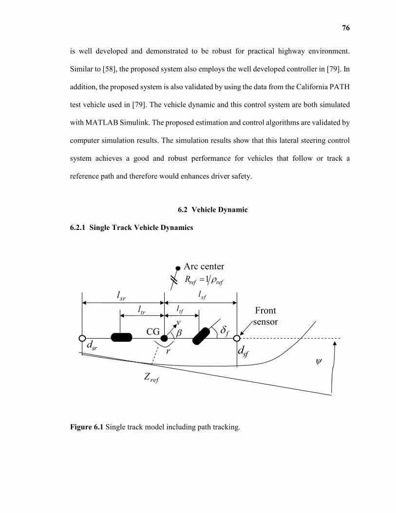
76
is well developed and demonstrated to be robust for practical highway environment.
Similar to [58], the proposed system also employs the well developed controller in [79]. In
addition, the proposed system is also validated by using the data from the California PATH
test vehicle used in [79]. The vehicle dynamic and this control system are both simulated
with MATLAB Simulink. The proposed estimation and control algorithms are validated by
computer simulation results. The simulation results show that this lateral steering control
system achieves a good and robust performance for vehicles that follow or track a
reference path and therefore would enhances driver safety.
6.2 Vehicle Dynamic
6.2.1 Single Track Vehicle Dynamics
Figure 6.1 Single track model including path tracking.
Arc center
Front
sensor
ψsfdsrd
r
refZ
1ref refR ρ=
srl sfl
trl tfl
v
β fδCG
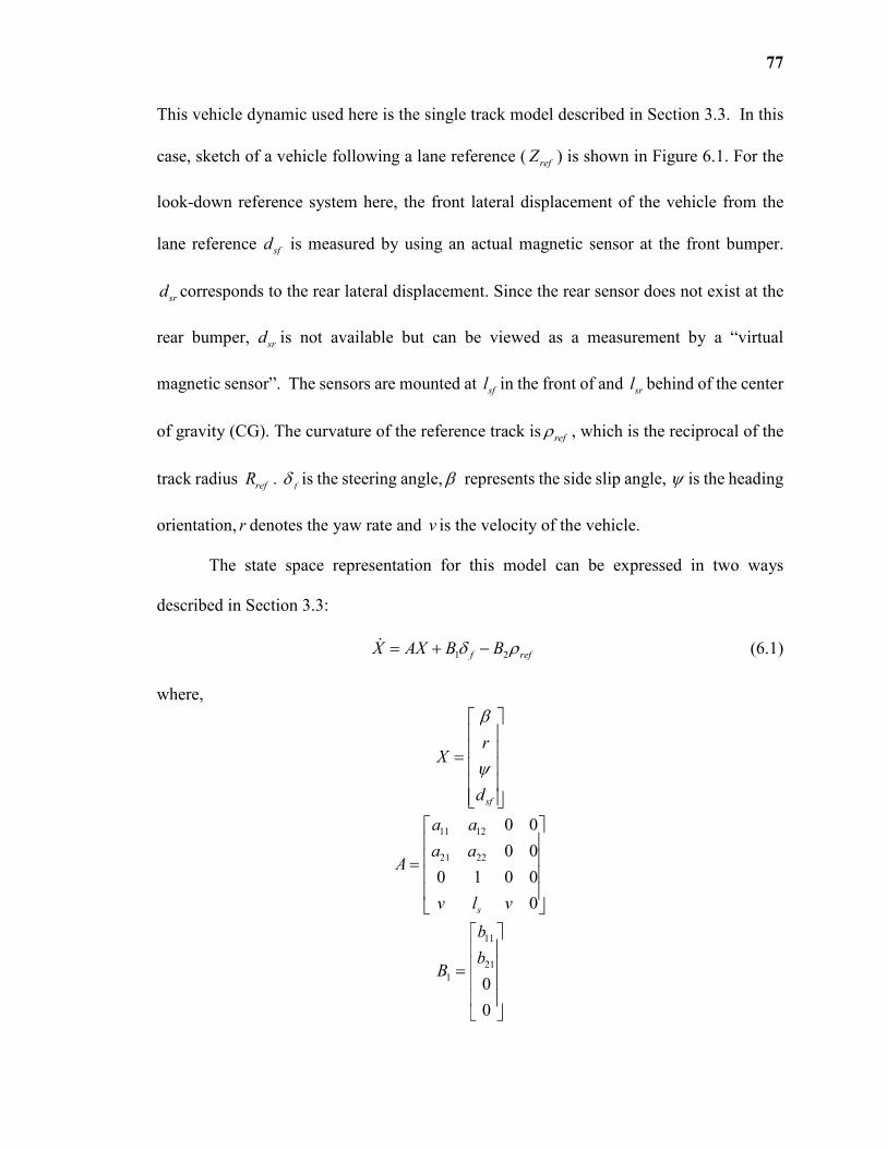
77
This vehicle dynamic used here is the single track model described in Section 3.3. In this
case, sketch of a vehicle following a lane reference ( refZ ) is shown in Figure 6.1. For the
look-down reference system here, the front lateral displacement of the vehicle from the
lane reference sfd is measured by using an actual magnetic sensor at the front bumper.
srd corresponds to the rear lateral displacement. Since the rear sensor does not exist at the
rear bumper, srd is not available but can be viewed as a measurement by a “virtual
magnetic sensor”. The sensors are mounted at sfl in the front of and srl behind of the center
of gravity (CG). The curvature of the reference track is refρ , which is the reciprocal of the
track radius refR . f
δ is the steering angle, β represents the side slip angle, ψ is the heading
orientation, r denotes the yaw rate and v is the velocity of the vehicle.
The state space representation for this model can be expressed in two ways
described in Section 3.3:
1 2f refX AX B Bδ ρ= + −ɺ (6.1)
where,
sf
rX
d
β
ψ
=
求
11 12
21 22
0 0
0 0
0 1 0 0
0s
a a
a aA
v l v
=
11
21
10
0
b
bB
=
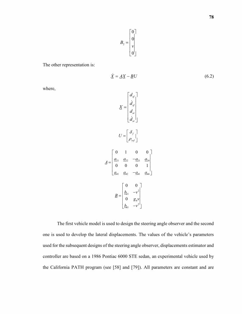
78
2
0
0
0
Bv
=
The other representation is:
X AX BU= −ɺ (6.2)
where,
sf
sf
sr
sr
d
dX
d
d
=
ɺ
ɺ
f
ref
Uδρ
=
21 22 21 24
41 42 41 44
0 1 0 0
0 0 0 1
a a a aA
a a a a
− =
−
2
21
4
2
41
0 0
0
b vB
g v
b v
− =
−
The first vehicle model is used to design the steering angle observer and the second
one is used to develop the lateral displacements. The values of the vehicle’s parameters
used for the subsequent designs of the steering angle observer, displacements estimator and
controller are based on a 1986 Pontiac 6000 STE sedan, an experimental vehicle used by
the California PATH program (see [58] and [79]). All parameters are constant and are
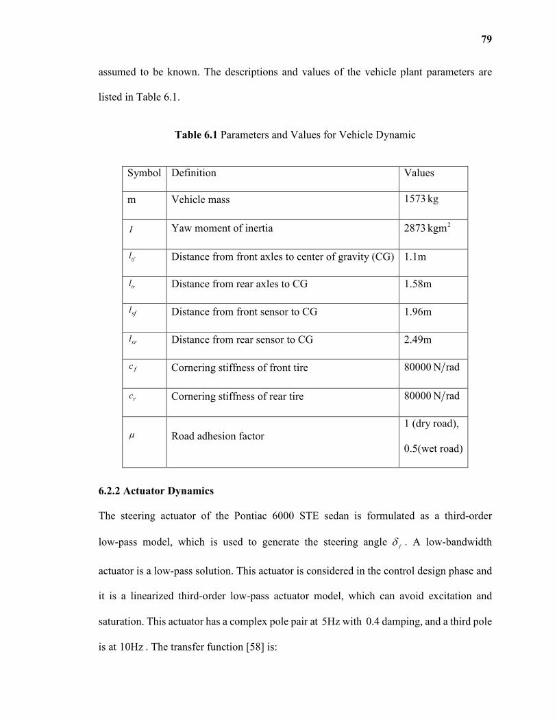
79
assumed to be known. The descriptions and values of the vehicle plant parameters are
listed in Table 6.1.
Table 6.1 Parameters and Values for Vehicle Dynamic
Symbol Definition Values
m Vehicle mass 1573 kg
I Yaw moment of inertia 2873 2kgm
tfl Distance from front axles to center of gravity (CG) 1.1m
trl Distance from rear axles to CG 1.58m
sfl Distance from front sensor to CG 1.96m
srl Distance from rear sensor to CG 2.49m
fc Cornering stiffness of front tire 80000 N rad
rc Cornering stiffness of rear tire 80000 N rad
µ Road adhesion factor
1 (dry road),
0.5(wet road)
6.2.2 Actuator Dynamics
The steering actuator of the Pontiac 6000 STE sedan is formulated as a third-order
low-pass model, which is used to generate the steering angle f
δ . A low-bandwidth
actuator is a low-pass solution. This actuator is considered in the control design phase and
it is a linearized third-order low-pass actuator model, which can avoid excitation and
saturation. This actuator has a complex pole pair at 5Hz with 0.4 damping, and a third pole
is at 10Hz . The transfer function [58] is:
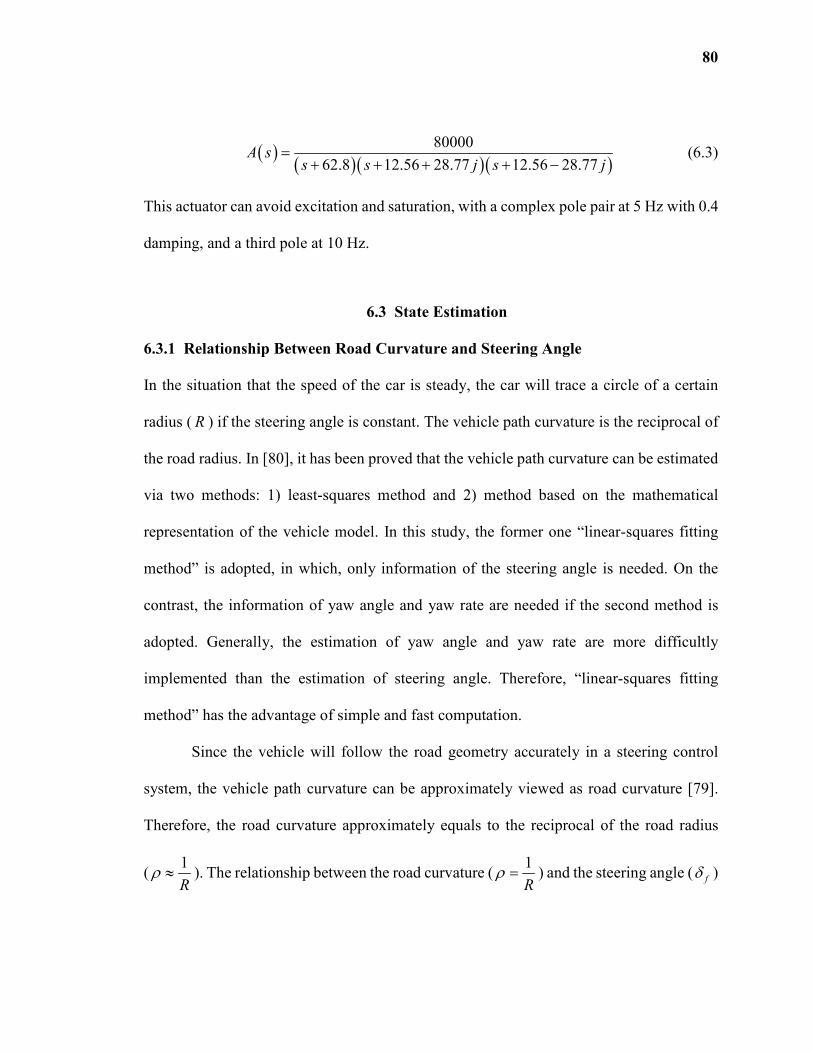
80
( )( )( )( )
80000
62.8 12.56 28.77 12.56 28.77A s
s s j s j=
+ + + + − (6.3)
This actuator can avoid excitation and saturation, with a complex pole pair at 5 Hz with 0.4
damping, and a third pole at 10 Hz.
6.3 State Estimation
6.3.1 Relationship Between Road Curvature and Steering Angle
In the situation that the speed of the car is steady, the car will trace a circle of a certain
radius ( R ) if the steering angle is constant. The vehicle path curvature is the reciprocal of
the road radius. In [80], it has been proved that the vehicle path curvature can be estimated
via two methods: 1) least-squares method and 2) method based on the mathematical
representation of the vehicle model. In this study, the former one “linear-squares fitting
method” is adopted, in which, only information of the steering angle is needed. On the
contrast, the information of yaw angle and yaw rate are needed if the second method is
adopted. Generally, the estimation of yaw angle and yaw rate are more difficultly
implemented than the estimation of steering angle. Therefore, “linear-squares fitting
method” has the advantage of simple and fast computation.
Since the vehicle will follow the road geometry accurately in a steering control
system, the vehicle path curvature can be approximately viewed as road curvature [79].
Therefore, the road curvature approximately equals to the reciprocal of the road radius
(1
Rρ ≈ ). The relationship between the road curvature (
1
Rρ = ) and the steering angle ( fδ )
81
is nearly a straight line according to [80] and the above approximation. It can be
approximated as
fρ α γδ= + (6.4)
where, parameters α and γ are the constant parameters.
α and β can be determined through repeated independent simulations repeated for
.many times (say, 500 times). On the one hand, the vehicle model used in the simulation
only employs the first two variables ( β and r ) in equation (6.1). Therefore, the steering
angle f
δ is the only input. Therefore, the front wheel steering angle f
δ is the only input.
The subsystem of the model of equation (6.1) is:
11 12 11
21 22 21
f
a a b
a a brr
ββδ
= +
ɺ
ɺ (6.5)
The coordinates of the vehicle position to further calculate the values of the road curvature
ρ is introduced. The derivative of the vehicle position coordinates are:
cosX v β=ɺ (6.6)
sinY v β=ɺ (6.7)
Therefore, the entire vehicle dynamic is formed from the combination of equations (6.5) -
(6.7) with the following nonlinear state space representation:
11 12 11
21 22 21
cos 0
sin 0
f
a a r b
a a r br
vX
vY
βββ
δββ
+ + = +
ɺ
ɺ
ɺ
ɺ
(6.8)
The road curvature can be calculated by the following expression:
2 2
1 1
R X Yρ = =
+ (6.9)
82
During the independent simulations, the values of the steering angle f
δ are
randomly sampled. Based on the road curvature and the steering angle experimental data
used or obtained in those independent simulations, the unknown parameters α and γ can
be calculated by using the linear least squares estimation method [81]. Then, the linear
relationship between the road curvature and the steering angle is determined. If the steering
angle is already estimated ( ˆfδ ), the road curvature estimation ρ is realized according to
their linear relationship:
ˆˆfρ α γδ= + (6.10)
6.3.2 Steering Angle Estimation
Consider the front displacementsfd and the heading angleψ as the outputs of the model in
equation. (6.1), the plant is described as:
1 2f refX AX B Bδ ρ= + −ɺ (6.11)
CX=y
with
0 0 1 0
0 0 0 1C
=
sfd
ψ =
y .
It is assumed that the second-order derivative of the steering angle is zero
( 0fδ =ɺɺ ). The reference road curvature input adopts the linear expression
ref fρ α γδ= + (6.12)
83
Furthermore, two additional state variables are introduced: the first-order and
second-orderfδ and fδɺ . The model in equation (6.1) is then extended to a new six-order
system which has no input signal:
E E E EΧ = Α Χ −Β (6.13)
E E= Χy C
with
E
fsf
ff
f
rX
d
β
ψδδ
δ
δ
Χ = =
ɺ
ɺ
1 2 4 1
4 1
4 1
0 1
0 0
E
A B Bγ ×
×
×
− Α =
0
0
0
2
0
0
E
Bα Β =
2 1 2 1
E C × ×= C 0 0
sfd
ψ =
y .
X , A , 1B and 2B defined in equation. (6.1) and C is defined in equation. (6.11).
Since the steering angle f
δ is currently one of the state variables, its value can be
estimated by a state observer. Such continuous-time observer for the six-order extended
model (equation (6.13)) has the following structure:
84
( )ˆ ˆ ˆE E E E E ELΧ = Α Χ −Β + − Χy Cɺ
(6.14)
ˆ EΧ is the estimation of the vehicle states:
ˆˆˆ ˆˆ ˆˆT
E
sf f fr dβ ψ δ δ Χ = ɺ (6.15)
The continuous-time vector y is produced by two first-order holds used to interpolate the
discrete measurement vector *y .
*ψ corresponds to the discrete measurement of the
vehicle’s heading angle from the GPS and *
sfd is the discrete measurement of the vehicle’s
front lateral displacement.
sfd
ψ =
y (6.16)
*
*
*
sfd
ψ =
y (6.17)
In real life situation, *
sfd is the discrete measurement from the front sensor.
However, *ψ is not the direct measurement of the heading angle from the GPS since the
measurements of the heading angle provided by the GPS are values in the geographic
coordinate system. In order to obtain the heading angle for the vehicle coordinate system
*ψ , the GSP measurement of the heading angle at the initial point of a vehicle (origin of
the vehicle coordinate plane) should be used as a reference. For example, *ψ is the
difference of the GPS measurements of the heading angle between the current position and
the origin of a vehicle. During simulation, *
sfd is a simulated discrete value of the vehicle’s
front lateral displacement. It is assumed that the GPS measurement of the heading angle for
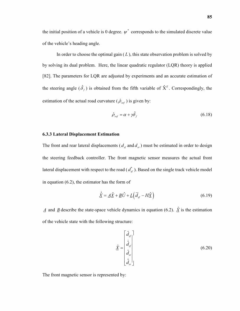
85
the initial position of a vehicle is 0 degree. *ψ corresponds to the simulated discrete value
of the vehicle’s heading angle.
In order to choose the optimal gain ( L ), this state observation problem is solved by
by solving its dual problem. Here, the linear quadratic regulator (LQR) theory is applied
[82]. The parameters for LQR are adjusted by experiments and an accurate estimation of
the steering angle ( ˆfδ ) is obtained from the fifth variable of ˆ EΧ . Correspondingly, the
estimation of the actual road curvature ( ˆrefρ ) is given by:
ˆˆref fρ α γδ= + (6.18)
6.3.3 Lateral Displacement Estimation
The front and rear lateral displacements (sfd and srd ) must be estimated in order to design
the steering feedback controller. The front magnetic sensor measures the actual front
lateral displacement with respect to the road (*
sfd ). Based on the single track vehicle model
in equation (6.2), the estimator has the form of
( )ˆ ˆ ˆ ˆsfX AX BU L d HX= + + −ɺ
(6.19)
A and B describe the state-space vehicle dynamics in equation (6.2). X is the estimation
of the vehicle state with the following structure:
ˆ
ˆˆ
ˆ
ˆ
sf
sf
sr
sr
d
dX
d
d
=
ɺ
ɺ
(6.20)
The front magnetic sensor is represented by:

86
[ ]1 0 0 0H = (6.21)
U is composed of an estimation of the steering angle ( ˆfδ ) and the actual road curvature
( ˆrefρ ), and they are provided by the estimators in Section 6.3.2.
ˆˆ
ˆ
f
ref
Uδρ
=
(6.22)
sfd is the output of a first-order hold used to interpolate the discrete measurements of the
front lateral displacement provided by front sensor (*
sfd ).
The proportional gain L is defined as:
[ ]1 1 1 1L l= (6.23)
and is chosen to achieve a small estimation error. The value l is gain scheduled related to
the vehicle velocity [19].
The estimator in equation (6.19) allows for the estimation of the front and rear
lateral displacements ( ˆsfd and ˆ
srd ). Note that the estimated ˆsfd can be viewed as the actual
measurement from the front sensor, which physically exists. And, the estimated ˆsrd is the
measurement from a “virtual rear sensor”, which does not physically exist.
6.4 Lateral Control Design
6.4.1 System Block Diagram
A block diagram of the lateral steering control system is shown in Figure 6.2. The single
track vehicle dynamic, steering actuator and feedback controller are described in Section
6.2.1, Section 6.2.2 and Section 6.4.2.
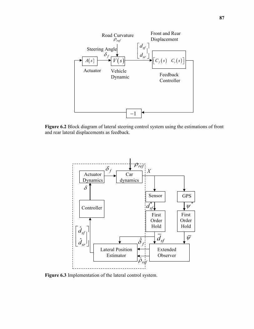
87
Figure 6.2 Block diagram of lateral steering control system using the estimations of front
and rear lateral displacements as feedback.
Figure 6.3 Implementation of the lateral control system.
Actuator
Dynamics
Car
dynamics
Sensor GPS
First
Order
Hold
First
Order Hold
Extended
Observer
Lateral Position
Estimator
Controller
*sfd
*ψ
ψ
sfdˆfδ
ˆrefρ
ˆ
ˆ
sf
sr
d
d
δ
fδ Xrefρ
( )A s ( )V sfδ
refρ
Vehicle
Dynamic
( ) ( )f rC s C s
sf
sr
d
d
Feedback
Controller
1−
Actuator
Steering Angle
Road Curvature Front and Rear
Displacement
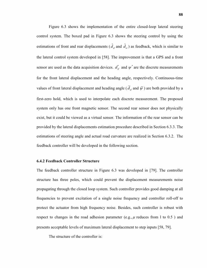
88
Figure 6.3 shows the implementation of the entire closed-loop lateral steering
control system. The boxed pad in Figure 6.3 shows the steering control by using the
estimations of front and rear displacements ( ˆsfd and ˆ
srd ) as feedback, which is similar to
the lateral control system developed in [58]. The improvement is that a GPS and a front
sensor are used as the data acquisition devices. *
sfd and *ψ are the discrete measurements
for the front lateral displacement and the heading angle, respectively. Continuous-time
values of front lateral displacement and heading angle ( sfd and ψ ) are both provided by a
first-zero hold, which is used to interpolate each discrete measurement. The proposed
system only has one front magnetic sensor. The second rear sensor does not physically
exist, but it could be viewed as a virtual sensor. The information of the rear sensor can be
provided by the lateral displacements estimation procedure described in Section 6.3.3. The
estimations of steering angle and actual road curvature are realized in Section 6.3.2. The
feedback controller will be developed in the following section.
6.4.2 Feedback Controller Structure
The feedback controller structure in Figure 6.3 was developed in [79]. The controller
structure has three poles, which could prevent the displacement measurements noise
propagating through the closed loop system. Such controller provides good damping at all
frequencies to prevent excitation of a single noise frequency and controller roll-off to
protect the actuator from high frequency noise. Besides, such controller is robust with
respect to changes in the road adhesion parameter (e.g., µ reduces from 1 to 0.5 ) and
presents acceptable levels of maximum lateral displacement to step inputs [58, 79].
The structure of the controller is:
89
( ) ( )f rC s C s (6.24)
where,
( )( ) ( )
2
2 2
2 1 11 2 1
f f fDD D P If
K s K s K KC s
ss s D sω ω ω
+ += +
+ + +
( )( ) ( )
2
2 2
2 1 11 2 1
r r rDD D P
r
K s K s KC s
s s D sω ω ω
+ +=
+ + +
The parameters of the controller structure are chosen as:
• Denominator poles :
1 2 4ω ω π= = .
• Damping factor:
0.8D = .
• Integral gain:
0.1IK = ;
• Zeros and the steady-state gains of ( )fC s :
0.0001fDDK = ,
0.087fD
K = ,
0.51fP
K = ,
• Zeros and the steady-state gains of ( )rC s :
0DDrK = ,
90
0.024DrK = − ,
0.28PrK = − .
6.5. Simulation Results
The state estimator and feedback controller design shown in Figure 6.3 is implemented and
tested with the data from the Pontiac 6000 STE sedan in the MATLAB Simulink
environment. The plant parameters used are listed in Table 6.1. A GPS is carried in the
vehicle and it is assumed that the sampling rate is 1 second. A magnetic sensor is installed
at the front bumper and the sampling rate for all simulations is 1second . In order to test the
robustness of the controller for actual situations, the simulations of the GPS and the
magnetic sensor signals are carried out by introducing additive white Gaussian noise
(AWGN). The measuring noise of the GPS is a normal distribution with mean of 0 degree
and variance of 1 2degree or ( )0,1N . The measuring noise of the displacement sensor is a
normal distribution with mean of 0cm and variance of 2
1cm or ( )0,1N .
The vehicle’s reference path consists of a straight section, a right turn followed by a
left turn, another right turn and finally a straight section. There are no transitions between
the curves to obtain the step response. The radius of each turn is 800mrefR = , which
means that the road curvatures for each turn is 31.25 10 / mrefρ −= × . The simulation time is
for 60s . This road curvature map of the reference track is shown in Figure 6.4. In the
following simulations, four different test cases with speeds of 45mi/hv = ( 20 m/sv = ) and
80mi/hv = ( 35.56 m/sv = , a highway speed) are considered, respectively, on a dry road
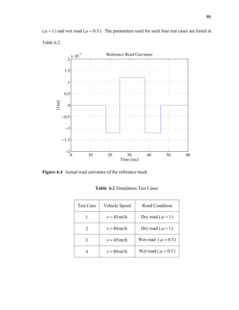
91
( 1µ = ) and wet road ( 0.5µ = ). The parameters used for such four test cases are listed in
Table 6.2.
0 10 20 30 40 50 60−2
−1.5
−1
−0.5
0
0.5
1
1.5
2x 10
−3
Time [sec]
[1/m
]Reference Road Curvature
Figure 6.4 Actual road curvature of the reference track.
Table 6.2 Simulation Test Cases
Test Case Vehicle Speed Road Condition
1 45mi/hv = Dry road ( 1µ = )
2 80mi/hv = Dry road ( 1µ = )
3 45mi/hv = Wet road ( 0.5µ = )
4 80mi/hv = Wet road ( 0.5µ = )
92
Based on the mathematical representation of the vehicle models in (6.1) and (6.2),
the observer is with respect to the vehicle’s linear velocity and road adhesion. The observer
becomes time-varying if the velocity and road adhesion are time-varying. However, the
observer can be considered as time-invariant in the case that the velocity and road adhesion
are constant. In this study, four cases are simulated under two different speeds and two road
adhesion conditions (Table 6.2). For each simulation case, the vehicle speed and road
adhesion are kept at constant values. Therefore, the observer gain can be fixed a-priori
before each simulation. The realization of the observers is as follows:
1) The observer gains ( L and L ) are properly pre-selected before each simulation
case based on certain constant speed and road adhesion factor.
2) During each simulation case, the vehicle speed and road factor are kept at
constant values. Then, the observer gains ( L and L ) are fixed.
This realization method is also employed in [58].
Figure 6.5 shows the controller performance on a dry road with a speed at
45mi/hv = . The estimation results of both steering angle and road curvature are within the
accuracy specifications. The RMSE value of steering angle estimation is 8.84% and the
RMSE value of road curvature estimation is 9.98%. Both of these two estimates are quite
accurate. The yaw rate is under an acceptable level. The lateral displacement control result
has no overshoot and is well damped. This simulation result yields a very small maximum
vehicle lateral displacement (steady state error is approximately0.1m ), which shows an
extremely accurate road tracking performance.
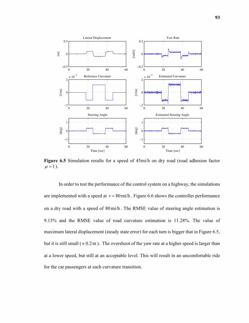
93
0 20 40 60−0.5
0
0.5
[m]
Lateral Displacement
0 20 40 60−0.2
0
0.2
[rad
/s]
Yaw Rate
0 20 40 60−2
0
2x 10
−3
[1/m
]
Reference Curvature
0 20 40 60−2
0
2x 10
−3
[1/m
]
Estimated Curvature
0 20 40 60
−1
0
1
Time [sec]
[deg
]
Steering Angle
0 20 40 60
−1
0
1
Time [sec]
[deg
]
Estimated Steering Angle
Figure 6.5 Simulation results for a speed of 45mi/h on dry road (road adhesion factor
1µ = ).
In order to test the performance of the control system on a highway, the simulations
are implemented with a speed at 80mi/hv = . Figure 6.6 shows the controller performance
on a dry road with a speed of 80 mi/h . The RMSE value of steering angle estimation is
9.13% and the RMSE value of road curvature estimation is 11.28%. The value of
maximum lateral displacement (steady state error) for each turn is bigger that in Figure 6.5,
but it is still small ( 0.2m≈ ). The overshoot of the yaw rate at a higher speed is larger than
at a lower speed, but still at an acceptable level. This will result in an uncomfortable ride
for the car passengers at each curvature transition.
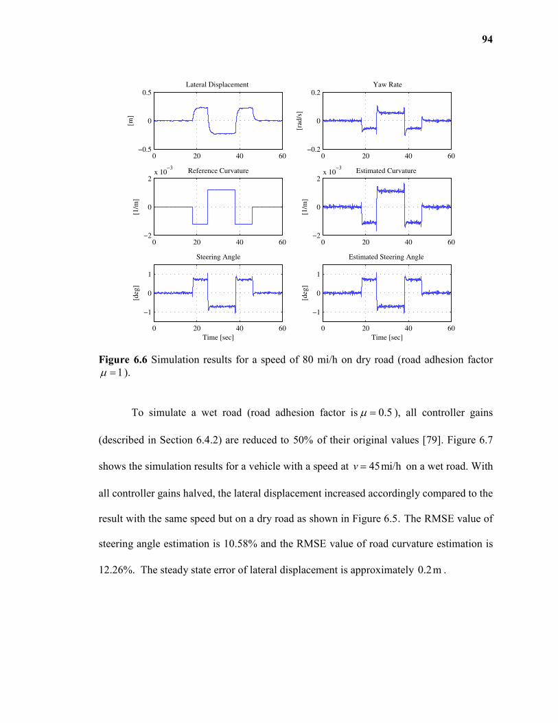
94
0 20 40 60−0.5
0
0.5
[m]
Lateral Displacement
0 20 40 60−0.2
0
0.2
[rad
/s]
Yaw Rate
0 20 40 60−2
0
2x 10
−3
[1/m
]
Reference Curvature
0 20 40 60−2
0
2x 10
−3
[1/m
]
Estimated Curvature
0 20 40 60
−1
0
1
Time [sec]
[deg
]
Steering Angle
0 20 40 60
−1
0
1
Time [sec]
[deg
]
Estimated Steering Angle
Figure 6.6 Simulation results for a speed of 80 mi/h on dry road (road adhesion factor
1µ = ).
To simulate a wet road (road adhesion factor is 0.5µ = ), all controller gains
(described in Section 6.4.2) are reduced to 50% of their original values [79]. Figure 6.7
shows the simulation results for a vehicle with a speed at 45mi/hv = on a wet road. With
all controller gains halved, the lateral displacement increased accordingly compared to the
result with the same speed but on a dry road as shown in Figure 6.5. The RMSE value of
steering angle estimation is 10.58% and the RMSE value of road curvature estimation is
12.26%. The steady state error of lateral displacement is approximately 0.2m .
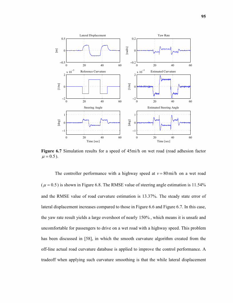
95
0 20 40 60−0.5
0
0.5
[m]
Lateral Displacement
0 20 40 60−0.2
0
0.2
[rad
/s]
Yaw Rate
0 20 40 60−2
0
2x 10
−3
[1/m
]
Reference Curvature
0 20 40 60−2
0
2x 10
−3
[1/m
]
Estimated Curvature
0 20 40 60
−1
0
1
Time [sec]
[deg
]
Steering Angle
0 20 40 60
−1
0
1
Time [sec]
[deg
]
Estimated Steering Angle
Figure 6.7 Simulation results for a speed of 45mi/h on wet road (road adhesion factor
0.5µ = ).
The controller performance with a highway speed at 80mi/hv = on a wet road
( 0.5µ = ) is shown in Figure 6.8. The RMSE value of steering angle estimation is 11.54%
and the RMSE value of road curvature estimation is 13.37%. The steady state error of
lateral displacement increases compared to those in Figure 6.6 and Figure 6.7. In this case,
the yaw rate result yields a large overshoot of nearly 150% , which means it is unsafe and
uncomfortable for passengers to drive on a wet road with a highway speed. This problem
has been discussed in [58], in which the smooth curvature algorithm created from the
off-line actual road curvature database is applied to improve the control performance. A
tradeoff when applying such curvature smoothing is that the while lateral displacement
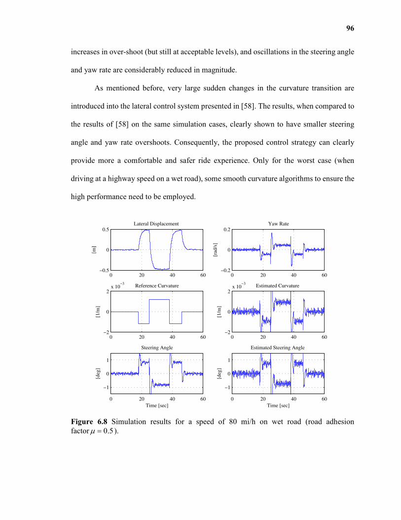
96
increases in over-shoot (but still at acceptable levels), and oscillations in the steering angle
and yaw rate are considerably reduced in magnitude.
As mentioned before, very large sudden changes in the curvature transition are
introduced into the lateral control system presented in [58]. The results, when compared to
the results of [58] on the same simulation cases, clearly shown to have smaller steering
angle and yaw rate overshoots. Consequently, the proposed control strategy can clearly
provide more a comfortable and safer ride experience. Only for the worst case (when
driving at a highway speed on a wet road), some smooth curvature algorithms to ensure the
high performance need to be employed.
0 20 40 60−0.5
0
0.5
[m]
Lateral Displacement
0 20 40 60−0.2
0
0.2
[rad
/s]
Yaw Rate
0 20 40 60−2
0
2x 10
−3
[1/m
]
Reference Curvature
0 20 40 60−2
0
2x 10
−3
[1/m
]
Estimated Curvature
0 20 40 60
−1
0
1
Time [sec]
[deg
]
Steering Angle
0 20 40 60
−1
0
1
Time [sec]
[deg
]
Estimated Steering Angle
Figure 6.8 Simulation results for a speed of 80 mi/h on wet road (road adhesion
factor 0.5µ = ).
97
6.6. Summary
This chapter investigates the automatic steering control for passenger vehicle. By using a
GPS and a front magnetic sensor, a novel look-down reference lateral control system is
developed. In such a system, accurate and real-time estimations of the steering angle, road
curvature, and vehicle’s front and rear lateral displacement are accomplished. The
performance of the steering angle extended observer, displacement estimation module and
the feedback controller is validated by simulation results. The results show that the
proposed steering control system is effective enough to be used for the automated steering
control both on dry and wet road under a high vehicle speed. This application could be used
in advanced driver assistance systems, such as lane keeping system, path control system,
collision avoidance system, and so on. This system could enhance the safety of driving.
98
CHAPTER 7
CONCLUSIONS AND FUTURE WORK
7.1 Conclusions
With the availability of low-cost GPS and other low cost sensors, this dissertation
investigates the use of such devices to develop vehicle state estimation, driver behavior
classification, and lateral control technologies which are needed in advanced driver
assistance systems. Since these low cost devices can only provide limited driving
information, the driver dynamics and kinemics are employed to estimate the vehicle states
and the driver behaviors.
For the vehicle state estimation, a task to estimate the longitudinal tire force which
can be transferred to the corresponding throttle/brake positions is addressed. A low cost
1Hz GPS receiver and a steering angle sensor are used as the vehicle data acquisition
equipment. A longitude force estimation scenario is developed for the nonlinear extended
two-wheel vehicle dynamic model using only the GPS information. The sideslip angle and
the yaw rate are estimated and an optimization scheme is proposed to estimate the
longitude tire force. The estimation results validate the proposed method by comparing
with the reference longitude tire force command.
For the driver behavior classification scenario, GPS data are employed to reproduce
the driver behavior. Gaussian Mixture model (GMM) is used to capture the sequence of
driving characteristics according to the reconstructed vehicle’s information and it is also
used as a classifier to assign the driving behavior into normal or abnormal category. The
nonlinear extended two-wheel vehicle dynamic model is adopted in this study. Two states,
99
i.e., the sideslip angle and the yaw rate are calculated, a piecewise optimization scheme is
proposed to reconstruct the driving behaviors which include the steering angle and the
longitude force. A GMM classifier is applied to identify whether the driver is under an
abnormal driving situation. This application can enhance the safety of the drivers by
warning drivers of the potentially dangerous traffic situations.
Controlling a vehicle requires the ability to measure or estimate its motion and to
determine parameters such as the vehicle states and vehicle displacements. As a
fundamental building block for the vehicle lateral control work, a GPS-based approach to
estimate in real time the necessary states and model parameters (the steering angle, road
curvature, and lateral displacements) has been developed. The control strategy used is a
look-down reference system which uses a sensor at the front bumper to measure the lateral
displacement and a GPS to measure the heading orientation. The road curvature estimator
is designed based on the steering angle. The steering angles are estimated by using the
sensor and the GPS information. The estimation algorithm employed is an observer for a
new extended system model, in which the steering angle and its derivative are viewed as
two state variables. Then, the lateral displacements estimation and the control algorithm
are investigated. An accurate and real-time estimation of the lateral displacements with
respect to the road can be accomplished in such a control system. The closed loop
controller is used as a compensator to control the lateral dynamics of the vehicle. The
vehicle dynamic and control system are simulated with MATLAB Simulink. The proposed
estimation and control algorithms are validated by simulation results. The results show that
the system provides a good and robust performance for path tracking.
100
7.2 Future Work
Based on the current studies, the near future work of interest would include:
1) Developing tire force estimation algorithm for four-wheel nonlinear vehicle
model.
Four-wheel nonlinear vehicle model is a more accurate model since it considers
both the lateral and longitudinal motions. On the one hand, the lateral tire forces are usually
modeled as linear with respect to lateral sideslip angle (λ ) for each axle (front and rear):
( ) , 1,2lateral i i iF C iλ λ= =
where iC is the wheel cornering stiffness, a parameter closely related to the tire-road
friction. Therefore, effective algorithms for estimating cornering stiffness need to be
developed. On the other hand, the longitudinal tire force for four-wheel nonlinear model is
determined by longitudinal motion (sideslip angle, velocity and acceleration). The vehicle
longitudinal motion is related to the vehicle dynamics and kinematics. The algorithm
presented in this dissertation for the four-wheel model should be further considered.
2) Developing driver state detection algorithm for the proposed GMM
classification method.
In this dissertation, the GMM classifier for abnormal driver behavior is
investigated. However, driver state (distraction or fatigue) is difficult to assess and detect
by using the driver inputs features. More driver data and features should be extracted to
detect the driver’s state. For instance, the distractions that are linked to the eye movements
and biological signals, such as ECG or EOG, are good indicator of fatigue. Future study
can include the driver’s state analysis into the proposed GMM scenario.
3) Designing smooth algorithms for lateral control system.

101
Since the lateral control system proposed in this study is based on estimated road
curvature, the sudden changes in curvature transition on the road will result in undesirable
levels of fluctuations in the lateral acceleration and the yaw rate. This will result in a poor
riding comfort to the passengers in the car. A smoothing algorithm could be used to
decrease their overshoots by providing smoother curvature changes. In the future, a
corresponding smoothing algorithm can be introduced into the control loop.
102
REFERENCES
1. “Our Nation’s Highways,” U.S. Department of Transportation, Federal Highway
Administration, FHWA-PL-10-023, 2010.
2. J. Wang, R. Knipling, and M. J. Goodman. “The role of driver inattention in crashes:
New statistics from the 1995 crashworthiness data system (CDS),” the 40th
Annual Proceedings: Association for the Advancement of Automotive Medicine,
1995.
3. “Early Estimate of Motor Vehicle Traffic Fatalities for The First Half (January-June)
of 2010,” U.S. Department of Transportation, National Highway Traffic Safety
Administration (NHTSA), DOT HS 811 403, September 2010.
4. “Motor Vehicle Traffic Crashes As a Leading Cause of Death in the United States
2005,” U.S. Department of Transportation, National Highway Traffic Safety
Administration (NHTSA), DOT HS 810 936, April 2008.
5. H. Lum and J. A. Reagan, “Interactive Highway Safety Design Model: Accident
Predictive Module,” Public Roads Magazine.
6. “Road Casualties Great Britain,” UK Department for Transport. April 13, 2008.
7. J. D., Lee, “Driving safety,” In R. S. Nickerson (Ed.), Review of Human Factors. Santa
Monica, CA: Human Factors and Ergonomics Society.
8. [Online]. Available: www.en.wikipedia.org/wiki/Traffic_collision, 2012.
9. K., Ball, and C. Owsley, “The useful field of view test: A new technique for evaluating
age-related declines in visual function,” Journal of the American Optometric
Association, 64, 71-79, 1993.
10. C. Owsley, K. Ball, G. McGwin, M. E. Sloane, D. L. Roenker, and M. F., White,
“Visual processing impairment and risk of motor vehicle crash among older
adults,” Journal of the American Medical Association, 279(14), 1083-1088,
1998.
11. T. A. Ranney, “Driver Distraction: A Review of the Current State-of-Knowledge,”
U.S. Department of Transportation, National Highway Traffic Safety
Administration (NHTSA), DOT HS 810 704, 2008.
12. “Advanced Driver Assistance System (ADAS): Vehicle Control for the Future,”
IMechE (Institution of Mechanical Engineers), December 1999.
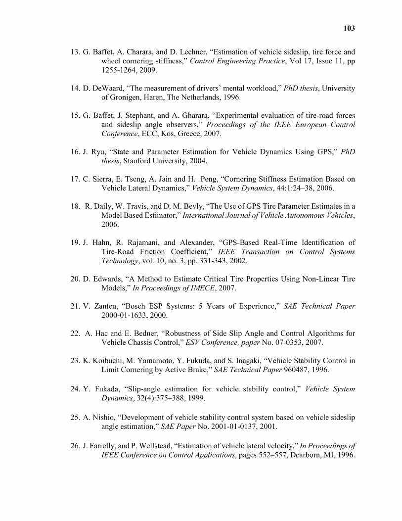
103
13. G. Baffet, A. Charara, and D. Lechner, “Estimation of vehicle sideslip, tire force and
wheel cornering stiffness,” Control Engineering Practice, Vol 17, Issue 11, pp
1255-1264, 2009.
14. D. DeWaard, “The measurement of drivers’ mental workload,” PhD thesis, University
of Gronigen, Haren, The Netherlands, 1996.
15. G. Baffet, J. Stephant, and A. Gharara, “Experimental evaluation of tire-road forces
and sideslip angle observers,” Proceedings of the IEEE European Control
Conference, ECC, Kos, Greece, 2007.
16. J. Ryu, “State and Parameter Estimation for Vehicle Dynamics Using GPS,” PhD
thesis, Stanford University, 2004.
17. C. Sierra, E. Tseng, A. Jain and H. Peng, “Cornering Stiffness Estimation Based on
Vehicle Lateral Dynamics,” Vehicle System Dynamics, 44:1:24–38, 2006.
18. R. Daily, W. Travis, and D. M. Bevly, “The Use of GPS Tire Parameter Estimates in a
Model Based Estimator,” International Journal of Vehicle Autonomous Vehicles,
2006.
19. J. Hahn, R. Rajamani, and Alexander, “GPS-Based Real-Time Identification of
Tire-Road Friction Coefficient,” IEEE Transaction on Control Systems
Technology, vol. 10, no. 3, pp. 331-343, 2002.
20. D. Edwards, “A Method to Estimate Critical Tire Properties Using Non-Linear Tire
Models,” In Proceedings of IMECE, 2007.
21. V. Zanten, “Bosch ESP Systems: 5 Years of Experience,” SAE Technical Paper
2000-01-1633, 2000.
22. A. Hac and E. Bedner, “Robustness of Side Slip Angle and Control Algorithms for
Vehicle Chassis Control,” ESV Conference, paper No. 07-0353, 2007.
23. K. Koibuchi, M. Yamamoto, Y. Fukuda, and S. Inagaki, “Vehicle Stability Control in
Limit Cornering by Active Brake,” SAE Technical Paper 960487, 1996.
24. Y. Fukada, “Slip-angle estimation for vehicle stability control,” Vehicle System
Dynamics, 32(4):375–388, 1999.
25. A. Nishio, “Development of vehicle stability control system based on vehicle sideslip
angle estimation,” SAE Paper No. 2001-01-0137, 2001.
26. J. Farrelly, and P. Wellstead, “Estimation of vehicle lateral velocity,” In Proceedings of
IEEE Conference on Control Applications, pages 552–557, Dearborn, MI, 1996.
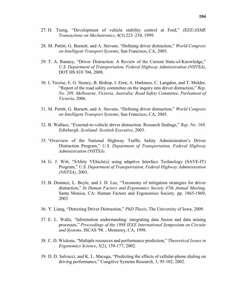
104
27. H. Tseng, “Development of vehicle stability control at Ford,” IEEE/ASME
Transactions on Mechatronics, 4(3):223–234, 1999.
28. M. Pettitt, G. Burnett, and A. Stevens, “Defining driver distraction,” World Congress
on Intelligent Transport Systems, San Francisco, CA, 2005.
29. T. A. Ranney, “Driver Distraction: A Review of the Current State-of-Knowledge,”
U.S. Department of Transportation, Federal Highway Administration (NHTSA),
DOT HS 810 704, 2008.
30. I. Trezise, E. G. Stoney, B. Bishop, J. Eren, A. Harkness, C. Langdon, and T. Mulder,
“Report of the road safety committee on the inquiry into driver distraction,” Rep.
No. 209. Melbourne, Victoria, Australia: Road Safety Committee, Parliament of
Victoria, 2006.
31. M. Pettitt, G. Burnett, and A. Stevens, “Defining driver distraction,” World Congress
on Intelligent Transport Systems, San Francisco, CA, 2005.
32. B. Wallace, “External-to-vehicle driver distraction: Research findings,” Rep. No. 168.
Edinburgh, Scotland: Scottish Executive, 2003.
33. “Overview of the National Highway Traffic Safety Administration’s Driver
Distraction Program,” U.S. Department of Transportation, Federal Highway
Administration (NHTSA).
34. G. J. Witt, “SAfety VEhicle(s) using adaptive Interface Technology (SAVE-IT)
Program,” U.S. Department of Transportation, Federal Highway Administration
(NHTSA), 2003.
35. B. Donmez, L. Boyle, and J. D. Lee, “Taxonomy of mitigation strategies for driver
distraction,” In Human Factors and Ergonomics Society 47th Annual Meeting,
Santa Monica, CA: Human Factors and Ergonomics Society. pp. 1865-1869,
2003.
36. Y. Liang, “Detecting Driver Distraction,” PhD Thesis, The University of Iowa, 2009.
37. E. L. Waltz, “Information understanding: integrating data fusion and data mining
processes,” Proceedings of the 1998 IEEE International Symposium on Circuits
and Systems, ISCAS '98. , Monterey, CA, 1998.
38. C. D. Wickens, “Multiple resources and performance prediction,” Theoretical Issues in
Ergonomics Science, 3(2), 159-177, 2002.
39. D. D. Salvucci, and K. L. Macuga, “Predicting the effects of cellular-phone dialing on
driving performance,” Congitive Systems Research, 3, 95-102, 2002.
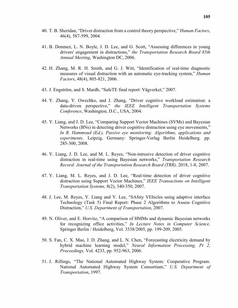
105
40. T. B. Sheridan, “Driver distraction from a control theory perspective,” Human Factors,
46(4), 587-599, 2004.
41. B. Donmez, L. N. Boyle, J. D. Lee, and G. Scott, “Assessing differences in young
drivers' engagement in distractions,” the Transportation Research Board 85th
Annual Meeting, Washington DC, 2006.
42. H. Zhang, M. R. H. Smith, and G. J. Witt, “Identification of real-time diagnostic
measures of visual distraction with an automatic eye-tracking system,” Human
Factors, 48(4), 805-821, 2006.
43. J. Engström, and S. Mardh, “SafeTE final report: Vägverket,” 2007.
44. Y. Zhang, Y. Owechko, and J. Zhang, “Driver cognitive workload estimation: a
data-driven perspective,” the IEEE Intelligent Transportation Systems
Conference, Washington, D.C., USA, 2004.
45. Y. Liang, and J. D. Lee, “Comparing Support Vector Machines (SVMs) and Bayesian
Networks (BNs) in detecting driver cognitive distraction using eye movements,”
In R. Hammoud (Ed.), Passive eye monitoring: Algorithms, applications and
experiments. Leipzig, Germany: Springer-Verlag Berlin Heidelberg. pp.
285-300, 2008.
46. Y. Liang, J. D. Lee, and M. L. Reyes, “Non-intrusive detection of driver cognitive
distraction in real-time using Bayesian networks,” Transportation Research
Record: Journal of the Transportation Research Board (TRR), 2018, 1-8, 2007.
47. Y. Liang, M. L. Reyes, and J. D. Lee, “Real-time detection of driver cognitive
distraction using Support Vector Machines,” IEEE Transactions on Intelligent
Transportation Systems, 8(2), 340-350, 2007.
48. J. Lee, M. Reyes, Y. Liang and Y. Lee, “SAfety VEhicles using adaptive interface
Technology (Task 5) Final Report: Phase 2 Algorithms to Assess Cognitive
Distraction,” U.S. Department of Transportation, 2007.
49. N. Oliver, and E. Horvitz, “A comparison of HMMs and dynamic Bayesian networks
for recognizing office activities,” In Lecture Notes in Computer Science,
Springer Berlin / Heidelberg, Vol. 3538/2005, pp. 199-209, 2005.
50. S. Fan, C. X. Mao, J. D. Zhang, and L. N. Chen, “Forecasting electricity demand by
hybrid machine learning model,” Neural Information Processing, Pt 2,
Proceedings, Vol. 4233, pp. 952-963, 2006.
51. J. Rillings, “The National Automated Highway System: Cooperative Program.
National Automated Highway System Consortium,” U.S. Department of
Transportation, 1997.
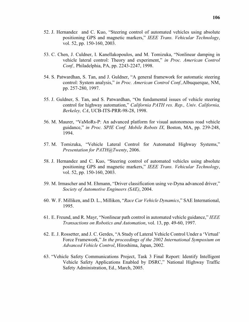
106
52. J. Hernandez and C. Kuo, “Steering control of automated vehicles using absolute
positioning GPS and magnetic markers,” IEEE Trans. Vehicular Technology,
vol. 52, pp. 150-160, 2003.
53. C. Chen, J. Culdner, I. Kanellakopoulos, and M. Tomizuka, “Nonlinear damping in
vehicle lateral control: Theory and experiment,” in Proc. American Control
Conf., Philadelphia, PA, pp. 2243-2247, 1998.
54. S. Patwardhan, S. Tan, and J. Guldner, “A general framework for automatic steering
control: System analysis,” in Proc. American Control Conf.,Albuquerque, NM,
pp. 257-280, 1997.
55. J. Guldner, S. Tan, and S. Patwardhan, “On fundamental issues of vehicle steering
control for highway automation,” California PATH res. Rep., Univ. California,
Berkeley, CA, UCB-ITS-PRR-98-28, 1998.
56. M. Maurer, “VaMoRs-P: An advanced platform for visual autonomous road vehicle
guidance,” in Proc. SPIE Conf. Mobile Robots IX, Boston, MA, pp. 239-248,
1994.
57. M. Tomizuka, “Vehicle Lateral Control for Automated Highway Systems,”
Presentation for PATH@Twenty, 2006.
58. J. Hernandez and C. Kuo, “Steering control of automated vehicles using absolute
positioning GPS and magnetic markers,” IEEE Trans. Vehicular Technology,
vol. 52, pp. 150-160, 2003.
59. M. Irmascher and M. Ehmann, “Driver classification using ve-Dyna advanced driver,”
Society of Automotive Engineers (SAE), 2004.
60. W. F. Milliken, and D. L., Milliken, “Race Car Vehicle Dynamics,” SAE International,
1995.
61. E. Freund, and R. Mayr, “Nonlinear path control in automated vehicle guidance,” IEEE
Transactions on Robotics and Automation, vol. 13, pp. 49-60, 1997.
62. E. J. Rossetter, and J. C. Gerdes, “A Study of Lateral Vehicle Control Under a ‘Virtual’
Force Framework,” In the proceedings of the 2002 International Symposium on
Advanced Vehicle Control, Hiroshima, Japan, 2002.
63. “Vehicle Safety Communications Project, Task 3 Final Report: Identify Intelligent
Vehicle Safety Applications Enabled by DSRC,” National Highway Traffic
Safety Administration, Ed., March, 2005.
107
64. A. A. Carter, “The status of vehicle-to-vehicle communications as a means of
improving crash prevention performance,” National Highway Traffic Safety
Administration, Ed.
65. Q. Xu, T. Mak, J. Ko and R. Sengupta, “Vehicle-to-vehicle safety messaging in
DSRC,” in Proceedings of the 1st ACM international workshop on Vehicular ad
hoc networks, ACM, 2004.
66. H. F. Grip, L. Imsland, T. A. Johansen, J. C. Kalkkuhl, and A. Suissa, “Vehicle sideslip
estimation,” Control Systems Magazine, IEEE, vol. 29, pp. 36-52, 2009.
67. L. R. Ray, “Nonlinear state and tire force estimation for advanced vehicle control,”
Control Systems Technology, IEEE Transactions on, vol. 3, pp. 117-124, 1995.
68. M. S., Grewal and A. P. Andrews, Kalman Filtering Theory and Practice. Upper
Saddle River, NJ: Prentice Hall, 1993.
69. J. D. Schutter, J. D. Geeter, T. Lefebvre and H. Bruyninckx, “Kalman Filters: A
Tutorial,” Technical report, 1999.
70. D. Titterington, A. Smith and U. Makov, “Statistical Analysis of Finite Mixture
Distributions,” John Wiley and Sons, 1985.
71. G. J. McLachlan and D. Peel, Finite Mixture Models, Wiley, 2000.
72. D. A. Reynolds, T. F. Quatieri, and R. B. Dunn, “Speaker verification using adapted
Gaussian Mixture Models,” Digital Signal Processing, vol. 10, pp 19–41, 2000.
73. F. Cardinaux, C. Cardinaux, and S. Marcel, “Comparison of MLP and GMM
Classifiers for Face Verification on XM2VTS,” Springer-Verlag GmbH, 2688,
pp. 911-920, 2003.
74. R. O. Duda and P. E. Hart, Pattern Classification and Sceneanalysis. John Wiley and
Sons, Inc. 1973.
75. P. Dempster, N. M. Laird and D. B. Rubin, “Maximum likelihood from incomplete
data using the EM algorithm,” Journal of the Royal Society of Statistics, vol.
39(1): pp. 1–38, 1977.
76. L. T. Lam, “Distraction and the risk of car crash injury: the effect of drivers’ age,” J.
Saf. Res., 33, pp. 411-419, 2002.
77. P. Angkititrakul, D. Kwak, S. Choi, J. Kim, A. PhucPhan, A. Sathyanarayana and J. H.
L. Hansen, “Getting Start with UTDrive: Driver-Behavior Modeling and
Assessment of Distraction for In-Vehicle Speech Systems,” Interspeech, 2007.
108
78. P. Green, “Driver Distraction, Telematics Design, and Workload Managers: Safety
Issues and Solutions,” SAE International, paper number: 2004-21-0022, 2004.
79. J. Guldner, W. Sienel, H. S. Tan, J. Ackermann, S. Patwardhan, and T. Bunte, “Robust
automatic steering control for look-down reference systems with front and rear
sensors,” IEEE Trans. Contr. Syst. Techno., vol. 7, pp. 2-11, 1999.
80. P. Mellodge, “Feedback control for path following robotics car,” Thesis, Virginia
Tech, 2002.
81. B. Ake, “Numerical methods for least squares problems,” Philadelphia: SIAM, 1996.
82. J. B. Burl, “Linear Optimal control,” Addison Wesley Longman edition, 1999.
83. Wikipedia: Geographic Distance. Web source: http://en.wikipedia.org/wiki/
Geographical_distance, 2012.
84. P. Dempster, N. M. Laird, and D. B. Rubin, “Maximum likelihood from incomplete
data using the EM algorithm,” Journal of the Royal Society of Statistics, vol.
39(1): pp. 1–38, 1977.
85. D. Karimi and D. D. Mann, “Role of visual cues from the environment in driving an
agricultural vehicle,” The Ergonomics Open Journal, pp. 54-61, 2008.
86. Y. Huang, K. B. Englehart, B. Hudgins, A. D. C. Chan, “Optimized Gaussian Mixture
Model for Upper Limb Motion Classification,” Proceeding of the 26th Annual
International Conference of the IEEE EMBS, San Francisco, CA, USA, 2004.
87. Wikipedia : Root mean square, Web source : http://en.wikipedia.org/wiki/
Root_mean_square, 2012.
88. C. Ahlstrom and K. Kircher, “Review of Real-time Visual Driver Distraction Detection
Algorithms,” Proceeding of Measuring Behavior, 2010.
89. O. Nakayama, T. Futami, and T. Nakamura, “Development of a steering entropy
method for evaluating driver workload,” SAE International, 1999.
90. B. Donmez, L. N. Boyle, J. D. Lee, and G. Scott, “Assessing differences in young
driver’s engagement in distractions,” The Transportation Research Board 85th
Annual Meeting, Washington DC, 2006.
91. H. Zhang, M. R. H. Smith, and G. J. Witt, “Identification of real-time diagnostic
measures of visual distraction with and automatic eye-tracking system,” Human
Factors, 48 (4), 805-821, 2006.
92. D. Karimi and D. D. Mann, “Role of visual cues from the environment in driving an
agricultural vehicle,” The Ergonomics Open Journal, pp. 54-61, 2008.
109
93. Y. Huang, K. B. Englehart, B. Hudgins, A. D. C. Chan, “Optimized Gaussian Mixture
Model for Upper Limb Motion Classification,” Proceeding of the 26th Annual
International Conference of the IEEE EMBS, San Francisco, CA, USA, pp.
72-75, Sept. 2004.
94. P. Green, “Driver Distraction, Telematics Design, and Workload Managers: Safety
Issues and Solutions,” SAE International, paper number : 2004-21-0022, 2004.
95. [Online]. Available: www.seeingmachines.com/product/facelab/, 2012.
96. T. A. Ranney, “Driver Distraction: A Review of the Current State-of-Knowledge,”
U.S. Department of Transportation, National Highway Traffic Safety
Administration (NHTSA), DOT HS 810 704, Apr. 2008.
97. B. Zylstra, O. Tsimhoni, P. Green, and K. Mayer, “SAfety VEhicles using Adaptive
Interface Technology (Task 3B): Driving Performance for Dialing, Radio,
Tuning, and Destination Entry while Driving Straight Roads,” U.S. Department
of Transportation, National Highway Traffic Safety Administration (NHTSA),
2004
98. H. Zhang, M. Smith, and R. Dufour, “A final report of SAFety Vehicles using adaptive
interface technology (Phase II: Task 7C): Visual Distraction,” U.S. Department
of Transportation, Federal Highway Administration (NHTSA), 2008
99. Y. Dong, Z. Hu, K. Uchimura, and N. Murayama, “Driver Inattention Monitoring
System for Intelligent Vehicles: A Review,” IEEE Trans. Intelligent
Transportation Systems, vol 12, no. 2, pp. 596-614, Jun. 2011.
100. O. M. J. Carsten and K. Brookhuis, “Issues arising from the haste experiments,”
Transp. Res. Part F: Traffic Psychol. Behavior, vol. 8, no. 2, pp 191- 196, 2005.
101. T. W. Victor, “Keeping eye and mind on the road,” in Dept of Psychology. Digital
Comprehensive Summaries of Uppsala Dissertation from the Faculty of Social
Sciences, Uppsala University: Uppsala, 2005.
102. L. Fletcher, and A. Zelinsky, “Driver State monitoring to mitigate distraction,”
International Conference on Driver Distraction. Sydney, Australia, 2005.
103. K. Kircher, and C. Ahlstrom, “Issues related to the driver distraction detection
algorithm,” 1st International Conference on Driver Distraction, Sydney,
Australia, Sept. 2009.
104. B. Donmez, L. N. Boyle, and J. D. Lee, “Safety implications of providing real-time
feedback to distracted drivers,” Accident Analysis and Prevention, 39, 3. pp.
581-590. 2007.
105. H. Zhang and M. Smith, “Safety Vehicles using adaptive Interface Technology (Task
7): A Literature Review of Visual Distraction Research,” The National Highway
Traffic Safety Administration (NHTSA),2004
110
106. “Overview of the National Highway Traffic Safety Administration’s Driver
Distraction Program,” U.S. Department of Transportation, Federal Highway
Administration (NHTSA).
107. J. L. Harbluk, Y. I. Noy, P. L. Trbovich, and M. Eizenman, “An on-road assessment of
cognitive distraction: Impacts on driver’s visual behavior and braking
performance,” Accid, Anal. Prev., vol. 39, no. 2, pp. 372-379, Mar. 2007.
108. E. M. Rantanen and J., Goldberg, “The effect of mental workload on the visual filed
size and shape,” Ergonomics, vol. 2, no. 6, pp. 816-834, 1999.
109. M. Miyaji, H. Kawanaka, and K. Oguri, “Driver’s cognitive distraction detection
using physiological features by the AdaBoost,” in Proc. 12th Int. IEEE Conf.
Intell. Transp. Syst. pp 1-6, St. Louis, Missouri, Oct. 2009.
110. M. C. Su, C. Y. Hsiung, and D. Y. Huang, “A simple approach to implementing a
system for monitoring driver inattention,” in Proc. IEEE Int. Conf. Syst., Man,
Cybern., vol. 1, pp 429-433, Taipei, Taiwan, 2006.
111. [Film]: A. Singer, The future of augmented cognition, DARPA, 2005
112. M. Itoh, “Individual differences in effects of secondary cognitive activity during
driving on temperature at the nose tip,” in Proc. IEEE Int. Conf. Mechatronics
Autom., pp. 7-11, Jinlin, China, Aug. 2009.
113. A. Wesley, D. Shastri, and I. Pavlidis, “A novel method to monitor driver’s
distractions,” in Proc. CHI, pp. 4273-4278, 2010.
114. K. Kircher, A. Kircher, and F. Claezon, “Distraction and drowsiness,” A field study,
VTI: Linkoping, 2009.
115. B. Donmez, L. N. Boyle, and J. D. Lee, Designing feedback to mitigate distraction, in
Driver Distraction: Theory, effects and mitigation, CRC Press London, 2009.
116. R. S. Michalski, J. G. Carboell, and T. M. Mitchell, Machine Learning: An Artificial
Intelligence Approach, Morgan Kaufmann Publishers, Inc. 1985.
117. A. Sathyanarayana, S, Nageswaren, H. Ghasemzadeh, R. Jafari, and J. H. L. Hansen,
“Body sensor networks for driver distraction identification,” IEEE International
Conference on Vehicular Electronics and Safety (ICVES), pp. 120-125,
Columbus, OH, Sept. 2008.
118. Y. Liang, and J. D. Lee, “Comparing Support Vector Machines (SVMs) and Bayesian
Networks (BNs) in detecting driver cognitive distraction using eye movements,”
In R. Hammoud (Ed.), Passive eye monitoring: Algorithms, applications and
experiments. Leipzig, Germany: Springer-Verlag Berlin Heidelberg. pp.
285-300, 2008.
111
119. Y. Liang, J. D. Lee, and M. L. Reyes, “Non-intrusive detection of driver cognitive
distraction in real-time using Bayesian networks,” Transportation Research
Record: Journal of the Transportation Research Board (TRR), 2018, 1-8. 2007.
120. Y. Zhang, Y. Owechko, and J. Zhang, “Driver cognitive workload estimation: a
data-driven perspective,” IEEE Intelligent Transportation Systems Conference,
Washington, D.C., USA. October 2004.
121. V. N. Vapnik, The nature of statistical learning theory, New York: Springer, 1995.
122. S. Amari, and S. Wu, “Improving support vector machine classifiers by modifying
kernel function,” Neural Networks, vol 12, pp. 783-789, 1999.
123. H. Byun, and S. W. Lee, “Applications of support vector machines for pattern
recognition: A survey,” the Pattern Recognition with Support Vector Machines:
First International Workshop, pp 213-236, Niagara Falls, Canada, August, 2002
124. Y. Liang, M. L. Reyes, and J. D. Lee, “Real-time detection of driver cognitive
distraction using Support Vector Machines,” IEEE Trans. on Intelligent
Transportation Systems, vol. 8, no. 2, pp. 340-350, 2007.
125. G. Weller and B. Schlag, “A robust method to detect driver distraction,” in
Proceeding of European Conference Human Centred Design for Intelligent
Transport. Systems, pp 279-288, Berlin, Germany, 2010.
126. D. Waard, K. A. Brookhuis, and N. Hernandez-Gress, “The feasibility of detecting
phone-use related driver distraction,” International Journal of Vehicle Design,
vol. 26, no.1, pp. 85-95, 2001.
127. M. Wollmer, C. Blaschke, T. Schindl, B. Schuller, B. Farber, S. Mayer, and B.
Trefflich “Online Driver Distraction Detection Using Long Short-Term
Memory,” Intelligent Transportation Systems, IEEE Transactions on , vol.12,
no.2, pp.574-582, Jun. 2011.
128. Y. Freund and R. E. Schapire, “A decision-theoretic generalization of online learning
and an application to boosting,” J. Comput. Syst. Sci,, vol. 55, no. 1, pp. 119-139,
1997.
129. Y. Freund and R. E. Schapire, “A short introduction to boosting,” Journal of Japanese
Society for Artificial Intelligence, 14(5): 771-780, 1999.
130. A. Sathyanarayana, P. Royraz, and J. H. Hansen, “Driver behavior analysis and route
recognition by hidden Markov models,” in Proc. IEEE Int. Conf. Veh. Electron.
Safety, pp. 267-281, Columbus, OH, 2008.
131. W. Stevens, “The automated highway system program: A progress report,” 13th IFAC
World Congr,, San Francisco, pp. 25-34, 1996.
112
132. S. Tsugawa, M. Aoki, A. Hosaka, and K. Seki, “A survey of present IVHS activities in
Japan,” in 13th IFAC World Congr,, San Francisco, CA, pp. 147-152, 1996.
133. Q. T. Luong, J. Weber, D. Koller, and J. Malik, “An integrated stereobased approach
to automatic vehicle guidance,” in Proc. 5th ICCV, Jun. 1995.
134. S. E. Shladover, “PATH at 20-History and Major Milestones,” IEEE Trans. Intell.
Transp. Syst., vol.8, no.4, pp.584-592, Dec. 2007.
135. B. Ulmer, “VITA - An autonomous road vehicle (ARV) for collision avoidance in
traffic,” in Proc. Intell. Veh, Detroit, pp. 36-41, 1992.
136. B. Ulmer, “VITA II – Active collision avoidance in real traffic,” in Proc. Intell.
Veh.’94, Paris, France, pp. 1-6, 1994.
137. T. Jochem, D. Pomerleau, B. Kumar, and J. Armstrong, “PANS: A portable
navigation platform,” in Proc. Intell. Veh. Symp., Detroit, MI, pp. 107-112, 1995.
138. W. Zhang and R.E.Parsons, “An intelligent roadway reference system for vehicle
lateral guidance/control,” in Proc. Amer. Contro. Conf., San Diego, CA, pp.
281-286, 1990.
139. R. E. Fenton, G.C. Melocik, and K. W. Olson, “On the steering of automated vehicles:
Theory and experiment,” IEEE Trans. Contr. Syst. Technol., vol. 5, pp. 127-134,
1997.
140. S. Choi, J. Kim, and D. Kwak, “Analysis and Classification of Driver Behavior using
In-Vehicle CAN-Bus Information,” Biennial Workshop on DSP for In-Vehicle
and Mobile Systems, Istanbul, Turkey, June 17-19, 2007 .
141. C. Miyajima, Y. Nishiwaki, K. Ozawa, T. Wakita, K. Itou, K. Takeda, F. Itakura,
“Driver Modeling Based on Driving Behavior and Its Evaluation in Driver
Identification,” Proceedings of the IEEE , vol.95, no.2, pp.427-437, Feb. 2007.
142. S. K. Benli, R. Duzagac and M. T. Eskill, “Driver recognition using Gaussian Mixture
Models and decision fusion techniques,” Advances in Computation and
Intelligence, Lecture Notes in Computer Science, vol. 5370, pp. 803-811, 2008.