Doppler and Angle of Arrival Estimation from Digitally Modulated Satellite Signals in
Passive RF Space Domain Awareness
Mohd Noor Islam, Thomas Q. Wang, Samuel Wade, Travis Bessell, Tim Spitzer, Jeremy
Hallett
Clearbox Systems Pty. Ltd., ACT, Australia.
ABSTRACT
Space Domain Awareness (SDA) or Space Situational Awareness (SSA) is crucial for maintaining custody of satellites
especially as the number of active satellites continues to increase rapidly. Passive Radio Frequency (RF) is a promising
technique that compliments traditional SDA sensors, including RADARs and telescopes. Passive RF sensors can
operate 24/7 in all weather conditions detecting transmissions from satellites across all orbital regimes. In a Passive
RF system, Doppler and Angle of Arrival (AoA) can be estimated from the received satellite signal. Satellites transmit
payload or Telemetry, Tracking and Command (TT&C) data using different modulation techniques, such as
Amplitude Shift Keying (ASK), Phase Shift Keying (PSK) and Frequency Shift Keying (FSK). The different
modulation techniques, combined with various line encoding, makes accurate Doppler and AoA estimation
challenging. This paper describes and implements a new technique based on Welch’s Power Spectral Density (PSD)
method to estimate the Doppler for a variety of modulated real satellite signals. The estimated Doppler is compared
to both Two Line Element (TLE) sets published by the 18th Space Control Squadron (18SPCS) and accurate
International Laser Ranging Service (ILRS) ephemeris data published by Crustal Dynamics Data Information System
(CDDIS). This paper also proposes an L-shaped planar antenna array to apply both the interferometer method and the
well-known Multiple Signal Classification (MUSIC) algorithm for AoA estimation. The AoA estimation is carried
out for an ASK modulated real satellite signal and compared against TLEs.
Keywords: Space Domain Awareness (SDA), Doppler, Angle of Arrival (AoA), Passive Radio Frequency (RF)
1. INTRODUCTION
Space assets are crucial to defence and civilian operations including weather monitoring, communications, and
positioning, navigation, and timing (PNT). In recent years, low cost of launch and the competition in private industries
on service-centred satellite constellations has caused space to become very congested, contested, and competitive. For
example, the enhancement of ridesharing capability has allowed a record breaking 143 spacecraft to be launched by a
single Falcon 9 rocket in 2021 with the previous record being 104 spacecraft by an Indian PSLV rocket in 2017 [1],
It is predicted that there will be about 50,000 satellites in space by the end of the next decade [2]. Therefore, increased
risk of collisions and a high threat posture between state actors, who want to leverage space, are two main challenges
to service providers soon and raises severe concern around Space Traffic Management (STM).
Space Domain Awareness (SDA) or Space Situational Awareness (SSA) provides a foundation for all space doctrine,
from protecting and defending space-based capabilities, to de-conflicting space traffic, to battle damage assessment.
These operations require accurate and timely SDA including reliable detection of objects and determination of the
intent of their activities to identify collision risks and threats. To date, SDA is primarily enabled by ground-based
radar, optical telescopes, and Satellite Laser Ranging (SLR). Current SDA platforms are incapable of handling the
future demand of uninterrupted monitoring due to their limitations. Ground-based RADAR technology is mainly
limited to Low Earth Orbit (LEO) and can only be extended at great cost. Optical telescopes and SLR are limited by
cloudy/rainy weather and/or daylight. Therefore, the SDA mission faces challenges for achieving 24/7 surveillance.
Passive Radio Frequency (RF) sensing technology for SDA leverages the transmitted signal from the satellite to
determine the satellite attributes and attitudes. RF spectrum monitoring and interference detection for satellite
communication technology is matured and has been a common practice for many years. Depending on the transmission
Copyright © 2021 Advanced Maui Optical and Space Surveillance Technologies Conference (AMOS) – www.amostech.com

frequency, satellite emissions are not substantially affected by weather or the time of day. Passive RF technology can
detect satellites at any range, so long as the satellite is transmitting over the area where a sensor is located. However,
passive RF sensors can only detect active satellites and therefore, passive RF technology can complement existing
SDA sensors in achieving an uninterrupted 24/7 surveillance in all weather conditions. Passive RF sensing can also
assist with identification of satellites based on their unique transmissions to prevent the cross-tagging problem that
can occur in traditional SDA sensors.
United States (US) based company, Kratos, has demonstrated passive RF technology through the repurposing of their
existing RF sensors to provide SDA monitoring for active satellites. The research has highlighted Passive RF’s
capability in determining GEO satellite manoeuvres [3,4,5]. In Europe, companies such as Zodiac GmbH and Siemens
AG are similarly looking to use their RF networks for SDA [6,7]. In Australia, the Murchison Widefield Array
(MWA), a precursor for the Square Kilometre Array (SKA) [8] mainly used for astrophysics and space weather, tested
an option of passive RF detection in 2015. Orbit determination of a LEO satellite using passive RF is still challenging
since they are only observable from a single ground location for a short period of time and often are only transmitting
intermittently. Passive RF sensors can generate observations on satellites in the form of Doppler [9], Angle of Arrival
(AoA), Time Difference of Arrival (TDoA) and Frequency Difference of Arrival (FDoA). These observations can be
used to estimate/infer aspects of the satellite such as determining its orbit.
Doppler is defined as the difference between observed and transmitted carrier frequencies. Satellite transmissions
includes Telemetry, Tracking and Command (TT&C) data and payload data such as communications, imagery, etc.
These transmissions may use different modulation techniques, such as Amplitude Shift Keying (ASK), Frequency
Shift Keying (FSK), Phase Shift Keying (PSK), etc. Different line coding techniques are also used to accommodate
both payloads and protocol signals in the approved frequency band. For example, SARAL uses BPSK with Manchester
line coding to accommodate PMT-A3 in the middle of the frequency band [10]. Again, CAS-4A uses A.25 protocol
signal in the middle of the two FSK carriers. PSK modulated signals span a spread of frequencies. Therefore, it’s
challenging to determine the true carrier frequency to estimate the Doppler.
This paper describes a new technique based on Welch’s Power Spectral Density (PSD) method [11] to estimate the
Doppler for a variety of modulated signals. Real data from satellites covering various modulated signals were captured
using Clearbox Systems’ Passive RF sensing network to verify the technique. The results were compared to both Two
Line Element (TLE) sets published by the 18th Space Control Squadron (18SPCS) [12] and accurate International
Laser Ranging Service (ILRS) ephemeris data published by Crustal Dynamics Data Information System (CDDIS)
[13].
Angle of Arrival (AoA) or Direction Finding (DF) is a common operation that is performed when detecting RF signals
in an antenna array [14]. Applying these techniques to satellite transmissions is challenging due to the faint signal
strength and intermittent transmissions. Using a low-cost L-shaped spatial planar array of three omni directional
antennas, it is possible to estimate the AoA of Low Earth Orbit (LEO) satellites as they pass overhead. Two techniques
including the interferometer method and the well-known Multiple Signal Classification (MUSIC) algorithm were
employed and compared. These techniques were applied to a satellite that was transmitting an ASK modulated signal.
The following section outlines the passive RF sensing system. In section 3, the Doppler and the angle of arrival (AoA)
estimation techniques are explained. Section 4 provides an overview of the passive RF sensors used to collect real
satellite data. Section 5 highlights the estimated Doppler and AoA results for real satellite data and the paper is
concluded in section 6.
2. PASSIVE RF SYSTEM
A typical Passive RF system consists of RF antennas/sensors, a signal digitisation unit, and a data processing unit as
presented in the block diagram shown in Fig. 1. Satellites make use of a wide range of frequencies bands from 30
MHz (VHF-band) to 40 GHz (Ka-band) and beyond.
The capability of a passive RF system is limited by the RF sensor/antenna selection in the RF frontend. Directional
antennas and motorised rotors can be used to receive signals with high gain, at the expense of having a narrower field
of view. Alternatively, omni-directional antennas can be used to sense satellite signals in a wide field of view but with
reduced capacity to sense lower power signals. Narrow band antennas have a higher probability to detect signals in
Copyright © 2021 Advanced Maui Optical and Space Surveillance Technologies Conference (AMOS) – www.amostech.com

areas with greater electromagnetic noise. Careful geographical placement of RF sensors can reduce noise and allow
wideband antennas to be used effectively to sense a wider variety of satellites, thereby reducing the cost to satellite
coverage ratio.
Fig. 1:Block Diagram for a Passive RF sensing system
The next important part of the passive RF system is the digitiser. Software Defined Radios (SDRs) are commonly
used to digitise RF signals as in-phase and quadrature components referred to as IQ data. The IQ data is then processed
in a Central Processing Unit (CPU)/Graphics Processing Unit (GPU) to extract information from the data. Data
processing complexity can be minimised when the signal capturing bandwidth is minimised and by distributing the
total band of interest in to different SDR channels. The SDA parameters including Doppler, Azimuth, Elevation, Time
Difference of Arrival (TDoA) and Frequency Difference of Arrival (FDoA) can be estimated from the IQ data.
3. DOPPLER AND ANGLE OF ARRIVAL
Satellites transmit data using various modulation techniques, such as ASK, FSK and PSK. The frequency spectrum of
received satellite signals are shown in Fig. 2 in green, which are (a) ASK modulated/CW signal from Max Valier Sat,
(b) GMSK modulated signal A.25 protocol signal in the middle of the FSK carriers transmitted from CAS-4A and (c)
BPSK signal transmitted by JY1SAT. SDA parameters such as Doppler and AoA are estimated based on the received
satellite signal and prior information of the satellite transmitter. Doppler estimation requires estimation of the carrier
frequency which is challenging due to the different modulation types. On the other hand, AoA estimation requires
signals from an array of antennas. Doppler and AoA estimation techniques are explained in this section.
(a) ASK Signal (Max Valier Sat) (b) GFSK A.25 signal (CAS-4A)
(c) BPSK signal (JY1SAT)
Fig. 2. FFT of various modulated signals and their power spectral density by Welch method.
Copyright © 2021 Advanced Maui Optical and Space Surveillance Technologies Conference (AMOS) – www.amostech.com

3.1 Doppler Analysis:
The Doppler frequency or Doppler shift is the difference between the transmitted and observed frequency,
𝑓𝑑 = 𝑓𝑜 − 𝑓𝑡, (1)
where, 𝑓𝑑 is the Doppler frequency, 𝑓𝑡 is the satellite transmitter frequency, and 𝑓𝑜 is the observed frequency. Since
the transmitted frequency 𝑓𝑡 is to be known, the Doppler shift depends on the accurate determination of the observed
frequency. In this paper, a generic method to determine the observed frequency 𝑓𝑜 of different modulated signals is
proposed. The method uses Welch method to smooth the frequency spectrum followed by a peak finding algorithm
determine the observed frequency. The frequency band can be represented by a single peak when the design
parameters of the Welch method is appropriately chosen.
Fig. 3. Welch Method analysis
Welch method [11] is a well-known technique that estimates the power spectral density by dividing the time signal
into successive blocks, forming the periodogram for each block, and then averaging over this block. In this paper, an
estimate of the observed frequency is performed for each second of data, Let 𝑁 represent the number of samples per
second as shown in Fig 3 and expressed as,
𝑦 = 𝑥[𝑗], where, 𝑗 = 0,1, … . . 𝑁 − 1, (2)
Let 𝜔(𝑛) represent a window, where 𝑛 = 0,1, … 𝑀 − 1, and the number of blocks in 𝑁 number of samples is 𝐾 shown
in Fig. 3. The 𝑚-th windowed, zero-padded frame from the signal 𝑥 can be expressed as,
𝑥𝑚(𝑛) = 𝜔(𝑛)𝑥(𝑛 + 𝑚𝑅), , 𝑚 = 0,1, … 𝐾 − 1. (3)
Where 𝑅 is defined as the window hop size. The periodogram of the 𝑚-th block is given by,
𝑃𝑥𝑚,𝑀(𝜔𝑘) =1
𝑀|𝐹𝐹𝑇𝑁,𝑘(𝑥𝑚)|
2=
1
𝑀|∑ 𝑥𝑚(𝑛)𝑀−1
𝑛=0 𝑒−𝑗2𝜋𝑛𝑘/𝑁|2 (4)
From this, the Welch estimate of the power spectral density is given by,
�̂�𝑥𝑊(𝜔𝑘) =
1
𝐾∑ 𝑃𝑥𝑚,𝑀(𝜔𝑘)𝐾−1
𝑚=0 (5)
Using the Welch method there is a tradeoff between bias and variance, where the following expression must hold,
𝑁 ≥ (𝐾 − 1)𝑅 + 𝑀 (6)
If no overlap is implemented (𝑅 = 𝑀), maximum independence is achieved where,
𝑁 ≥ 𝐾𝑀 (7)
Copyright © 2021 Advanced Maui Optical and Space Surveillance Technologies Conference (AMOS) – www.amostech.com
The bias of the output depends on the value of K and the variance depends on M. By increasing the block size 𝑀, the
spectral resolution can be maximized.
In applying the Welch method and detecting the peak for the observed frequency,𝑓𝑜, the value of 𝑀, the block size,
plays the main role. The prior information on data rate and the type of modulation are the main factors to determine
the value of 𝑀. For a low data rate, small bandwidth signal, the value 𝑀 should be large to enable higher resolution
and improved signal to noise ratio. For example, an ASK modulated / CW signal usually has very low data rate where
the higher value of 𝑀 can be used to resolve an accurate peak with great SNR using the peak finding algorithm which
is shown in Fig. 3(a). The similar 𝑀 value can also be chosen for FSK modulated signal as shown in Fig. 3(b).
However, for PSK, the high data rate signal causes frequencies to spread over a larger bandwidth, therefore, by
lowering the value of M the peak detection algorithm can resolve the center peak of the band. Fig. 3 (c) shows the
different outputs to the peak finding algorithm for large and small values of 𝑀.
3.2 Angle of Arrival Analysis
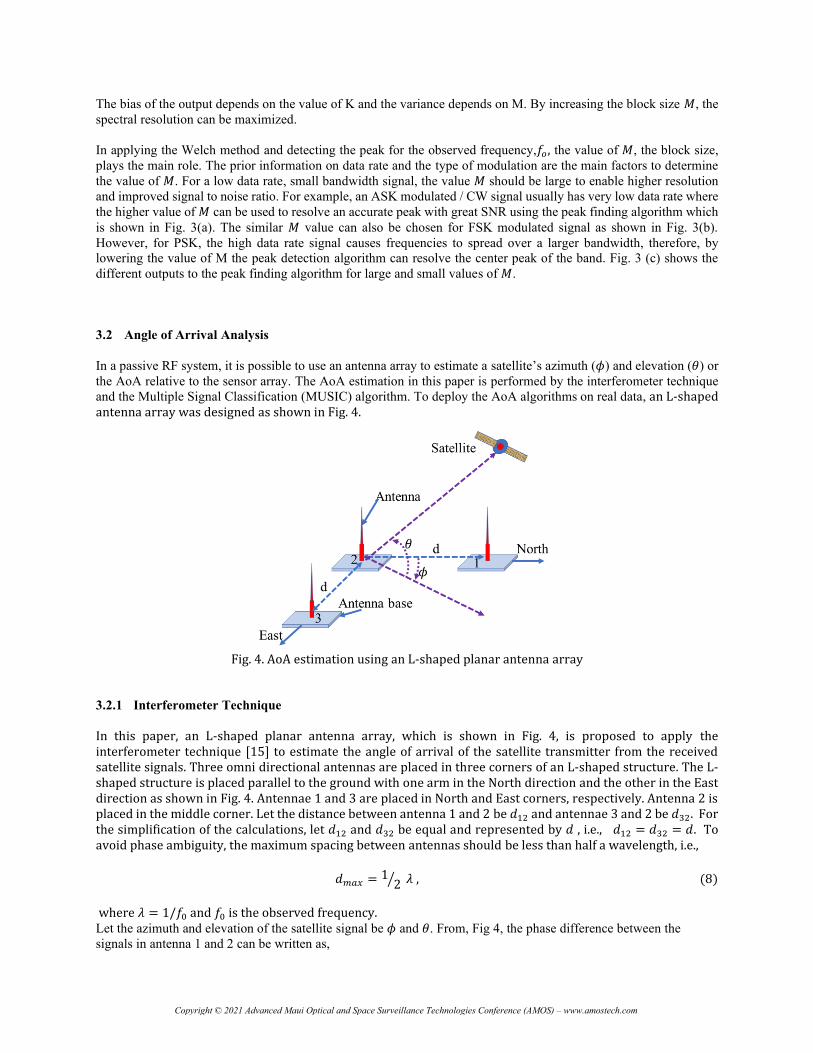
In a passive RF system, it is possible to use an antenna array to estimate a satellite’s azimuth (𝜙) and elevation (𝜃) or
the AoA relative to the sensor array. The AoA estimation in this paper is performed by the interferometer technique
and the Multiple Signal Classification (MUSIC) algorithm. To deploy the AoA algorithms on real data, an L-shaped antenna array was designed as shown in Fig. 4.
Fig. 4. AoA estimation using an L-shaped planar antenna array
3.2.1 Interferometer Technique
In this paper, an L-shaped planar antenna array, which is shown in Fig. 4, is proposed to apply the interferometer technique [15] to estimate the angle of arrival of the satellite transmitter from the received satellite signals. Three omni directional antennas are placed in three corners of an L-shaped structure. The L-shaped structure is placed parallel to the ground with one arm in the North direction and the other in the East direction as shown in Fig. 4. Antennae 1 and 3 are placed in North and East corners, respectively. Antenna 2 is placed in the middle corner. Let the distance between antenna 1 and 2 be 𝑑12 and antennae 3 and 2 be 𝑑32. For the simplification of the calculations, let 𝑑12 and 𝑑32 be equal and represented by 𝑑 , i.e., 𝑑12 = 𝑑32 = 𝑑. To avoid phase ambiguity, the maximum spacing between antennas should be less than half a wavelength, i.e.,
𝑑𝑚𝑎𝑥 = 12⁄ 𝜆 , (8)
where 𝜆 = 1/𝑓0 and 𝑓0 is the observed frequency. Let the azimuth and elevation of the satellite signal be 𝜙 and 𝜃. From, Fig 4, the phase difference between the
signals in antenna 1 and 2 can be written as,
Copyright © 2021 Advanced Maui Optical and Space Surveillance Technologies Conference (AMOS) – www.amostech.com

𝛾12 =𝑑12 2 𝜋
𝜆cos (𝜃)cos (𝜙) (9)
Again, the phase difference between antenna 2 and 3 can be written as,
𝛾32 =𝑑32 2 𝜋
𝜆cos (𝜃)sin (𝜙) (10)
From Equations (9) and (10), the azimuth (𝜙) and elevation (𝜃) can be derived as follows:
𝜙 = 𝑡𝑎𝑛−1(𝛾32𝑑12
𝛾12𝑑32) (11)
𝜃 = 𝑐𝑜𝑠−1(𝛾12 𝜆
2𝜋𝑑12cos (𝜙)) (12)
3.2.2 Multiple Signal Classification Algorithm
MUSIC is a common algorithm used for AoA estimation. It is based on the analysis of signal and noise spaces for the
received signal and makes use of the orthogonality between the spaces to search for the AoA [16]. When only one
source is assumed, the received signal can be expressed as
𝒚 = 𝒆𝑥 + 𝒏, (13)
where 𝒚, 𝒆, 𝑥 and 𝒏 denote the received signal, the steering vector, the signal received at the reference point and the
additive noise, respectively. Note that 𝒚, 𝒆 and 𝒏 are vectors with dimensions equaling the number of sensors, 𝑁𝑠. In
order to implement MUSIC algorithm, the following assumptions are made [17]:
(a) Signal 𝑥 is zero-mean with power 𝐸|𝑥|2 = 𝑃 . It is independent to the additive noise.
(b) The noise vector 𝒏 is zero-mean with independent elements, i.e., the additive noise in the sensors is
independent.
(c) The noise power, 𝜎2, is the same, but not necessarily available, for all the sensors.
Note that assumptions (a) and (b) are general in wireless communications systems. Assumption (c) is applicable in
most multi-antenna receivers. When the assumptions (b) and (c) do not hold in specific cases, the correlation matrix
of the noise will then be needed to whiten the signal.
Under the assumptions made above, the covariance matrix of the received signal can be expressed as
𝑹𝒚 = 𝑃𝒆𝒆𝐻 + 𝜎2𝑰 . (14)
As the term, 𝑃𝒆𝒆𝐻, is a Hermitian matrix with a unit rank, we can see that 𝒆 is one of its eigenvectors. To verify this,
we multiply 𝑃𝒆𝑒𝐻 with 𝒆 to have
𝑃𝒆𝒆𝐻𝒆 = (𝑃𝒆𝐻𝒆)𝒆. (15)
Eq. 15 also indicates that the eigenvalue corresponding to 𝒆 is 𝑃𝒆𝐻𝒆. As the rank of 𝑃𝒆𝒆𝐻 is one, the rest of its
eigenvalues are zero. The corresponding eigenvectors can be expressed as 𝒗1, … , 𝒗𝑁−1, which leads to
𝑃𝒆𝒆𝐻𝒗𝒊 = 𝟎, for 𝑖 = 1, … , 𝑁𝑠 − 1, (16)
where 𝟎 denotes the all-zero vector.
It is straightforward to prove that 𝒆 and 𝒗𝒊 are also eigenvectors of 𝑹𝒚. To verify this, we can see that
Copyright © 2021 Advanced Maui Optical and Space Surveillance Technologies Conference (AMOS) – www.amostech.com

𝑹𝒚𝒆 = (𝑃𝒆𝒆𝐻 + 𝜎2𝑰)𝒆 = (𝑃𝒆𝐻𝒆 + 𝜎2)𝒆 (17)
and
𝑹𝒚𝒗𝒊 = (𝑃𝒆𝒆𝐻 + 𝜎2𝑰)𝒗𝒊 = 𝜎2𝒗𝒊 (18)
The corresponding eigenvalues are 𝑃𝒆𝐻𝒆 and 𝜎2, respectively. In the statistical signal processing literature, the space
spanned by 𝒆 is defined to be the signal space, and 𝒗1, … , 𝒗𝑁−1 , the noise space. The two spaces are orthogonal to
each other.
Eq. 18 indicates that
(a) The noise power, 𝜎2, can be estimated by averaging the smallest 𝑁𝑠 − 1 eigenvalues.
(b) The steering vector 𝒆 can be estimated by using the eigenvector corresponding to the largest eigenvalue.
Eq. 17 indicates that after the noise power and steering vector are estimated, the signal power, 𝑃, can be estimated
from the largest eigenvalue.
When MUSIC algorithm is implemented for AoA estimation, the relationship between the AoA and steering vector 𝒆
is typically assumed known and depends on the geometry of the sensor array. For example, based on the configuration
of the sensors as shown in Fig. 4, the steering vector is given by
𝒆 = [𝑒𝑗2𝜋𝑑12
𝜆cos 𝜃 sin 𝜙, 1, 𝑒−𝑗
2𝜋𝑑32𝜆
cos 𝜃 cos 𝜙]𝑇 (19)
where 𝜃 and 𝜙 denote the elevation and azimuth angles, respectively.
As the covariance matrix, 𝑹𝒚, is Hermitian, the steering vector 𝒆 is orthogonal to the rest of the eigenvectors,
𝒗1, … , 𝒗𝑁−1. This forms the theoretical foundation of MUSIC algorithm. If forming a matrix 𝑽 that is made up from
the vectors, 𝒗1, … , 𝒗𝑁−1, i.e., 𝑽 = [𝒗1, … , 𝒗𝑁−1], then we can form the spatial spectrum, given by 1 𝒆𝐻𝑽𝑽𝐻𝒆⁄ . The
MUSIC algorithm then performs a search for the elevation and azimuth angles that lead to the maximum spatial
spectrum.
4. SATELLITE SIGNAL CAPTURING
Clearbox Systems has a passive RF sensor network across Australia. Satellite signals are captured from two sites
which are in Canberra (-35.292062,149.165202) and Adelaide (-35.106667, 138.518993), Australia. Those sites have
the capability for a range of frequency bands. Only the VHF and UHF capabilities have been used to capture signals
for this paper. They satellites included amateur radio satellites and an ILRS satellite named SARAL. The satellites are
listed in Table I, along with the transmitter information for each satellite. The signal from these satellites were used
to verify the Doppler and AoA estimation. The satellites were selected as they transmit signals using different
modulation techniques.
TABLE I: The list satellites and their on-board features.
Satellite Name Norad Id Transmitter
Modulation Signal Frequency
(MHz)
Data Rate
Max Valier Sat 42778 ASK Telemetry 145.961 12 baud
FALCONSAT-3 30776 FSK Transceiver 435.103 9k6
NAIF-1 42017 BPSK Telemetry
Beacon
145.940 1k2
SARAL 39086 BPSK PMT-A3 Telemetry 465.988 800 baud
N.B.: PMT-A3: Platform Messaging Transceiver-Argos-3, SARAL is one of the ILRS satellites.
Copyright © 2021 Advanced Maui Optical and Space Surveillance Technologies Conference (AMOS) – www.amostech.com

(a) Canberra site (b) Adelaide site
Fig. 4. L-shaped planar antenna arrays for Angle of Arrival (AoA)
The L-shaped VHF/UHF antenna arrays are shown in Fig. 4. Three SG-7900 omni directional antennas are used in
the antenna array. The antennas are connected to three channels of a four channel SDR (USRP x310) at each site.
Each channel is sampled at 500 kHz.
5. RESULTS AND ANALYSIS
Doppler and AoA are estimated based on theory explained in section 3. Doppler is estimated for ASK, FSK and PSK
modulated signals and compared with TLE and ILRS data. On the other hand, AoA is estimated only for ASK
modulated signal and compared with TLE data. The satellites whose signals are used for the analysis are tabulated in
Table I.
5.1 Doppler Estimation
The observed frequency and the Doppler frequency are estimated for the ASK modulated signal from Max Valier Sat
as listed in Table I. The data is captured from the Adelaide site for the pass starting at 2021-06-04T22:16:40Z and
ending at 2021-06-04T22:24:07Z. For each estimation, 500,000 samples are taken which is equal to the sample rate,
i.e., 𝑁 = 500𝑘. For this type of modulation, a block size of 𝑀 = 25000 was used with no overlap considered,
𝑅 = 𝑀. The estimated Doppler is compared with the derived Doppler from the TLE. The estimated Doppler is shown
in Fig. 5 along with the Doppler derived from the TLE. The difference between the estimated and derived Doppler
shifts are represented as a Doppler error also shown in Fig. 5. The root mean square (RMS) of Doppler error for the
duration of the capture is 3.04 Hz. It is observed from the figure that the mean of Doppler errors are non-zero and
changing over time, which is possibly due to the TLE error, as explained in section 5.1.1.
The observed frequency and the Doppler are estimated for an FSK modulated signal from FALCONSAT-3 as listed
in Table I. The data was captured from the Canberra site for the pass starting at 2021-03-07T23:22:52Z and ending at
2021-03-07T23:31:59Z. For each estimation, 500,000 samples are taken which is equal to the sample rate,
i.e., 𝑁 = 500𝑘 . For this type of modulation, a block size of 𝑀 = 2000 was used with no overlap considered, 𝑅 = 𝑀.
The estimated Doppler is compared with the derived Doppler from the TLE. The estimated Doppler is shown in Fig
6 along with the Doppler derived from the TLE. The difference between the estimated and derived Doppler shifts are
represented as the Doppler error shown in Fig. 6. The RMS of Doppler error for the duration of the capture is 66.55
Hz. For each estimation, the two peaks of the FSK carriers are first estimated then the center frequency is calculated.
Copyright © 2021 Advanced Maui Optical and Space Surveillance Technologies Conference (AMOS) – www.amostech.com

Fig. 5. Estimated Doppler and error compared to the TLE for the pass of Max Valier Sat starting at 2021-06-
04T22:16:40Z and ending at 2021-06-04T22:24:07Z captured from the Adelaide sensor site.
Fig. 6. Estimated Doppler and error compared to the TLE for the pass of FALCONSAT-3 starting at 2021-03-
07T23:22:52Z and ending at 2021-03-07T23:31:59Z captured from the Canberra sensor site.
The observed frequency and the Doppler are estimated for PSK modulated signal from NAIF-1 as listed in Table I.
The data is captured from the Canberra site for the pass starting at 2021-03-10T12:43:03Z and ending at 2021-03-
Copyright © 2021 Advanced Maui Optical and Space Surveillance Technologies Conference (AMOS) – www.amostech.com

10T12:51:52Z. For each estimation, 500,000 samples are taken which is equal to the sample rate,
Fig. 7. Estimated Doppler and error compared to the TLE for the pass of NAYIF-1 starting at 2021-03-
10T12:43:03Z and ending at 2021-03-10T12:51:52Z captured from the Canberra site.
i.e., 𝑁 = 500000. For this type of modulation, a block size of 𝑀 = 8000 was used with no overlap considered,
𝑅 = 𝑀. The estimated Doppler is compared with the derived Doppler from the TLE. The estimated Doppler is shown
in Fig 7 along with the Doppler derived from the TLE. The difference between the estimated and predicted Doppler
shifts is represented as the Doppler error in Fig. 7. The RMS value of Doppler error for the duration of the capture is
10.06 Hz. The variation of mean with time is due to the error in TLE which is later analysed comparing the estimates
with accurate ILRS data. From Fig. 7, it is clear that the estimated Doppler follows the center frequency of the
frequency band.
5.1.1 Comparison with ILSR data:
Signal from one of the International Laser Ranging Service (ILRS) satellites, SARAL, was captured from the sensor
sites to compare the Doppler to highly accurate ephemeris data. The signal captured from the Adelaide site for the
pass starting at 2021-05-24T20:00:37Z and ending at 2021-05-24T20:11:28Z is used to estimate the Doppler. For
each estimation, 500,000 samples are taken which is equal to the sample rate, i.e., 𝑁 = 500,000. For this modulation
type a block size of 𝑀 = 13000 was used with no overlap considered, 𝑅 = 𝑀.
Copyright © 2021 Advanced Maui Optical and Space Surveillance Technologies Conference (AMOS) – www.amostech.com

Fig. 8. Doppler comparison among ISLR, TLE and estimated for SARAL for the pass started at 2021-05-
24T20:00:37Z and ended at 2021-05-24T20:11:28Z from the Adelaide site.
The estimated Doppler and the calculated Doppler from the TLE are compared with the highly accurate Satellite Laser
Ranging (SLR) data provided by ILRS. The Doppler errors are shown in Fig. 8. The mean and standard deviation of
the Doppler estimates compared to the ILRS ephemeris are 0 Hz and 0.9 Hz respectively. When comparing the TLE
to the ILRS ephemeris the mean and standard deviation are-1.5814 Hz and 1.4159 Hz respectively. Based on this
result, the estimated Doppler is found to be more accurate than the given TLE. The estimated Doppler variation is less
and in the range of fraction of a hertz in the beginning and end of the pass while in the range of ±4 Hz in the middle
of the pass due to the rate of change of Doppler being its highest during the middle of the pass.
From this comparison with accurate SLR data, it has been demonstrated that the estimated Doppler from this method
is more accurate than the given TLE. When comparing the Doppler estimates with the TLE shown in Figs 5 and 7 the
means of the Doppler errors were varying with time. This analysis has indicated that this is due to TLE errors.
5.2 AoA Estimation
Both interferometer method and MUSIC algorithm have been implemented to estimate the azimuth (𝜙) and elevation
(𝜃) of a satellite signal. The AoA estimation is carried out for ASK modulated signal from Max Valier Sat as listed in
Table I. The three antennas of the array were connected to three channels of the SDR. The SDR channels are phase
synchronised and the phases for three RF chains from the antenna to the SDR are calibrated prior to digitising the
satellite signals to IQ data. The satellite signal is captured for the pass starting at 2021-06-04T22:16:40Z and ending
at 2021-06-04T22:24:07Z.
Copyright © 2021 Advanced Maui Optical and Space Surveillance Technologies Conference (AMOS) – www.amostech.com

Fig. 9. Phases estimation and compared to the TLE for the pass of Max Valier Sat starts at 2021-06-04T22:16:40Z
and ends at 2021-06-04T22:24:07Z
In the interferometer method, the phase differences between antennas 1 and 2 and antennas 2 and 3 are estimated in
two ways: (a) using cross-correlation method in time domain and (b) using the FFT magnitude and phase information
for the observed frequency. The estimated phases and the predicted phases from given TLE are shown in Fig. 9. The
RMS errors compared to the TLE for γ12 and 𝛾32 are calculated of 13.6 and 14 degrees, respectively. These angles
are used to estimate the azimuth (𝜙) and elevation (𝜃) based on the equations (11) and (12) which are shown in Fig.
10. The RMS errors of azimuth (𝜙) and elevation (𝜃) compared to TLE are 5.5 and 8.7 degrees, respectively.
Fig. 10. AoA estimation and compared to the TLE for the pass of Max Valier Sat starts at 2021-06-04T22:16:40Z
and ends at 2021-06-04T22:24:07Z
Copyright © 2021 Advanced Maui Optical and Space Surveillance Technologies Conference (AMOS) – www.amostech.com
Again, the azimuth and elevation angles are directly estimated using the MUSIC algorithm. The signal is filtered with
a bandpass filter of 200 Hz bandwidth around the observed frequency, 𝑓0 , i.e., 𝑓𝑜 ± 100, where 𝑓𝑜 is estimated by
welch method as explained in section 5.1, The covariance matrix, 𝑹𝒚, used in MUSIC algorithm is estimated as
expressed in eq. 14. The estimated azimuth (𝜙) and elevation (𝜃) by MUSIC algorithm are shown in Fig. 10. The
RMS azimuth and elevation errors compared to TLE are 6.7 and 7.9 degrees, respectively.
The results shown in Fig. 9 and 10 demonstrate that both interferometer and MUSIC algorithm are feasible techniques
for AoA estimation for LEO satellites and either method could be used for AoA estimation for ASK modulated signal.
From the Fig. 10, it is observed that the estimated azimuth is close to the predicted value, but the elevation is more
erroneous.
The AoA estimation uses signals from three antennas. Therefore, in AoA estimation, antennas, amplifiers, and cables
need to be identical, all the channels in the SDR need to be phase synchronised and each of the three antennas in the
array should receive signal equally. Again, AoA estimation is also sensitive to the mutual coupling between antennas
as it impacts the voltage induction in all three antennas. The errors in AoA arises may have different reasons, such as
(a) all the off-the-shelf components are used in the AoA experiment, which may not be identical,
(b) different mutual coupling between antennas as the distance among antennas are not equal,
(c) the orientation of the antenna in Max Valier Sat may changing over time,
(d) the signal to noise ratio (SNR) was not constant over the pass,
(e) multiple path fading may happen,
(f) some terrestrial signals are noticed in the frequency range in Adelaide site, and
(g) antenna array is constructed with minimum number of antennas and place horizontally on 2D-plane.
Some of these reasons have been investigated prior to the data being captured, however, the other reasons need more
investigation.
6. CONCLUSION AND FUTURE WORK
This paper describes and implements the Welch method in determining the Doppler for LEO satellites from their
signals consisting of a variety of modulation techniques. The accuracy of the estimated Doppler is found to be less
than a Hz compared to the accurate ILRS satellite laser ranging data. An L-shaped planar antenna array is proposed
for AoA estimation. Both the interferometer technique and MUSIC algorithm are applied to AoA determination for
an ASK modulated satellite signal. The estimated AoA is compared with the predicted AoA calculated from the TLE.
Future work will look to improve the accuracy of AoA estimation by increasing the number of antennas in the array
and by vertical placement of the array. The AoA estimation will also be extended to PSK and FSK modulated satellite
signals. Using the Doppler and AoA measurements orbit determination will also be investigated in future work.
7. ACKNOWLEDGEMENT
This research was conducted as part of an Australian Cooperative Research Centre Projects (CRC-P) led by Clearbox
Systems in collaboration with the University of New South Wales (UNSW). The authors would like to acknowledge
the support from the Australian Department of Industry, Science, Energy and Resources as well as the support from
UNSW Canberra for hosting a sensor site to enable real data to be collected.
Copyright © 2021 Advanced Maui Optical and Space Surveillance Technologies Conference (AMOS) – www.amostech.com

8. REFERENCES
[1] https://www.cnbc.com/2021/01/24/spacex-launches-rideshare-mission-with-143-spacecraft.html, cited on August
26, 2021.
[2] https://www.sda.mil/us-military-places-a-bet-on-leo-for-space-security/, cited on August 26, 2021. [3] https://www.kratosdefense.com/
[4] Matthew Prechtel, “Event Detection from RF Sensing.” 34th Space Symposium, Technical Track, Colorado
Springs, Colorado, United States of America, April, 2018.
[5] Kameron Simon, “Passive RF in Support of Closely Spaced Objects Scenarios”, In Advanced Maui Optical and
Space Surveillance (AMOS) Technologies Conference, September 2020. [6] Lal, Bhavya, et al. "Global trends in space situational awareness (SSA) and space traffic management (STM)."
Science and Technology Policy Institute (2018).
[7] Morreale, Brittany, Travis Bessell, Mark Rutten, and Brian Cheung. "Australian Space Situational Awareness Capability Demonstrations." In Advanced Maui Optical and Space Surveillance (AMOS) Technologies Conference, p. 63. 2017.
[8] Square Kilometre Array. 2018. “Participating Countries.” https://www.skatelescope.org/participating-countries/
[9] Islam, Mohd Noor, Tim Spitzer, Jeremy Hallett, and Md Asikuzzaman. "Doppler Estimation for Passive RF Sensing Method in Space Domain Awareness." In 2020 Military Communications and Information Systems Conference (MilCIS), pp. 1-4. IEEE, 2020.
[10] http://mdkenny.customer.netspace.net.au/ARGOS-3.pdf, cited on August 26, 2021.
[11] P. D. Welch, “The use of fast Fourier transforms for the estimation of power spectra: A method based on time
averaging over short modified periodograms,'' IEEE Transactions on Audio and Electroacoustics, vol. 15, pp. 70-
73, 1967 [12] https://www.space-track.org/, cited on August 26, 2021.
[13] https://cddis.nasa.gov/, cited on August 26, 2021.
[14] “Introduction into Theory of Direction Finding,” Rohde & Schwarz Radio monitoring & Radiolocation, Catalog
2010/2011
[15] Guo, Fucheng, Yun Fan, Yiyu Zhou, Caigen Xhou, and Qiang Li. Space electronic reconnaissance: localization
theories and methods. John Wiley & Sons, 2014.
[16] R. O. Schmidt, “Multiple Emitter Location and Signal Parameter Estimation,” IEEE Transactions on Antennas
and Propagation, vol. AP-34, no. 3, pp. 276-280, Mar. 1986.
[17] P. Stoica and A. Nehorai, “MUSIC, Maximum Likelihood, and Cramer-Rao Bound,” IEEE Transactions on
Acoustics, Speech, and Signal Processing, vol. 37, no. 5, pp. 720-741, May 1989.
Copyright © 2021 Advanced Maui Optical and Space Surveillance Technologies Conference (AMOS) – www.amostech.com