Electronic copy available at: http://ssrn.com/abstract=968871
1
Do Active Fund Managers Care About Capital Gains Tax Efficiency?
Kingsley Y.L. Fong*
David R. Gallagher†
Sarah S.W. Lau
Peter L. Swan‡
Australian School of Business, The University of New South Wales, Sydney NSW 2052 AUSTRALIA
Abstract:
This study investigates the tax efficiency of actively managed equity funds by conducting a previously unaddressed natural experiment. Specifically, we examine whether asset sales were timed to take advantage of the introduction of a substantial discount to realized capital gains when the holding period was at least one year. Institutional equity fund management in Australia is principally focused on the pre-fee and pre-tax performance surveys of leading asset consultants. Given this industry setting, our study is important because tax efficiency is not accounted for directly in the reported performance numbers, and is thus opaque. We find that active fund managers overall have significantly increased the proportion of long-term capital gains realized after the change in taxation code, although there are significant variations across funds. We also find that active fund managers realize more long-term gains on both large capitalization and low volatility stocks.
Keywords: portfolio management, capital gains tax, active management
JEL classification: G23
* Corresponding author. Banking and Finance, Australian School of Business, The University of New South Wales, Sydney, N.S.W. 2052 AUSTRALIA Tel: + 61 2 93854932, fax: + 61 2 93856347, e-mail: [email protected].. † David R. Gallagher. Email: [email protected]. I wish to thank the Australian Research Council (ARC) for financial support (DP0346064). ‡ Peter L. Swan. Email: [email protected]. I wish to thank the Australian Research Council (ARC) for financial support (DP0346064).

Electronic copy available at: http://ssrn.com/abstract=968871
2
1. Introduction
This study investigates actively managed equity funds’ tax efficiency by conducting a
previously unaddressed natural experiment – an examination of whether stock sales were
timed in order to take advantage of a 50 percent discount in taxable capital gains for assets
with a holding period of at least 12 months. The capital gains tax discount was introduced in
1999 through an amendment to the Income Tax Assessment Act. Applying the popular First-
In-First-Out (FIFO) principle to our sample of the daily trades of twenty-six institutional
equity funds from 1994 to 2002, we find the proportion of short-term capital gains realized
decreased in a statistically significant manner after the change in taxation code. The overall
decrease in the proportion of short-term capital gains is not evident when capital gains are
computed using the Last-In-First-Out (LIFO) methodology. However, the LIFO approach is
inherently insensitive to fund managers’ tax management.1
Commonly used investment funds (i.e., unit trusts) are not liable for taxation
themselves, however, fund income and realized capital gains are ‘passed through’ to unit
holders, where income tax is assessed at the individual investor level.2 The U.S. Securities
and Exchange Commission (SEC) mandate that mutual funds disclose the impact of tax
liabilities in mutual fund advertising and marketing materials. 3 However there are no
corresponding legal requirements in Australia. While fund performance is published and
monitored through the surveys of asset consultants and fund ratings houses as well as
contained in databases, the principal focus of the fund management industry has been on the
1 The method also results in undesirably large unrealized capital gains being accumulated and distributed to future fund investors. 2 There are taxable investment vehicles, which do pay tax as a collective investment scheme, such as pooled superannuation trusts and life office funds. However, the most commonly available investment scheme is that of a unit trust, which distributes income and capital gains to individual unit holders. 3 Rule 482 under the Securities Act of 1933 and rule 34b-1 under the Investment Company Act of 1940 which require certain funds to include standardized after-tax returns in advertisements and other sales material. These rules are effective from April 16, 2001 but the compliance date has been extended to December 1, 2001.

Electronic copy available at: http://ssrn.com/abstract=968871
3
collection and dissemination of pre-tax performance.4 Our findings are important in relation
to public policy concerns within the current fund manager reporting and performance survey
assessment regime. Arnott and Jeffrey (1993) and Arnott et al. (2000) highlight the
differences between before-tax and after-tax returns. Dickson and Shoven (1993) and
Mawani et al. (2003) argue that the relative rankings of funds can differ significantly between
before-tax and after-tax assessment criteria. Opponents of after-tax reporting argue that
differences in individual investors’ tax rates would lead to inconsistent reporting; including
the assertion that investors will not understand the impact of tax on total returns; and that
after-tax computations increases administration costs.5 While active fund managers argue
that it has been the norm over the past three years for Australian equity managers to carefully
monitor turnover, with respect to tax considerations,6 index fund managers argue that taxes
are neglected because active fund managers are not measured with respect to after-tax
returns.7 A potential conflict of interest exists when only pre-tax returns are published
because investors do not have an opportunity to compare the net returns among a peer group.
Fund managers may be executing “rash trades”8 to increase their pre-tax returns marginally,
but such activity may not necessarily maximize after-tax returns, nor be in the interests of
unit holders. Our findings suggest that not all Australian active fund managers are operating
in a way that optimizes the after tax returns for fund investors.
This study makes contributions to the literature that examines whether, and to what
extent, investors respond to tax incentives. Stiglitz (1983) and Constantinides (1983, 1984)
analyze the effect of taxes on investment decisions. They suggest that investors should
realize losses immediately and defer the realization of gains until a forced liquidation arises,
4 Dunstan (2006a). Index fund provider, Vanguard, and multi-manager MLC are the notable exceptions. 5 Barrett (2006b) 6 Wright (2006) 7 Dunstan (2006a) 8 Barrett (2006b).

4
in order to maximize the present value of tax shields and to minimize the present value of tax
liabilities. Gibson, Safieddine and Titman (2000), Poterba and Weisbenner (2001), and
Grinblatt and Keloharju (2004) find evidence that individual and institutional investors
increase the selling of loss-making stocks prior to the tax year end. However, there are
competing theories to this tax loss selling hypothesis that could explain fund manager tax
year end selling for loss-making stocks, such as the window dressing and seasonality (see
Grinblatt and Keloharju, 2004, and Sias, 2007). Our study of the capital gains tax discount
provides a unique and unambiguous event to test whether delegated fund trading is
responsive to the tax incentives of the principals-investors.
U.S. evidence suggests that investors are tax-aware and adjust their investment flows
to tax incentives, even before the SEC’s mandatory disclosure requirement. Bergstresser and
Poterba (2002) study the performance-flow relation with respect to after-tax returns, and
document that fund inflows are more sensitive to past period after-tax performance than is the
case for gross returns. Dickson et al. (2000) also find that funds with net inflow outperform
those with net outflow on an after-tax basis. Barclay, Pearson and Weisbach (1998) show
institutional funds with large unrealized capital gains (i.e., capital gains overhang) experience
lower fund inflows by comparison to other funds. Jin (2006) documents that the selling
decisions of U.S. institutions are indeed sensitive to the capital gains tax overhang for taxable
investors, in contrast to non-taxed investors. Our study extends this literature on tax
management within an industry which exhibits opacity of after-tax performance by
examining heterogeneity across fund styles and fund manager attributes. Our research also
examines the impact of a fund manager’s inventory system on the tax position of fund
investors. In addition, our study extends the literature through the use of a unique dataset of

5
daily trades and monthly portfolio holdings of a representative sample of Australian
institutional equity fund managers to examine fund trading at a transaction level.9
The remainder of this paper is structured as follows: section 2 reviews the literature
and section 3 outlines the Australian capital gains tax code. We describe the data in section 4
and conduct univariate tests in section 5. Section 6 provides a multivariate analysis, and we
conclude in section 7.
3. Capital gains tax in Australia
Capital gains tax became effective in Australian on September 19, 1985. A capital gain is
derived when an asset is sold (i.e. disposed) above its cost base, and the tax is levied at the
investor’s marginal tax rate. Before September 21, 1999, the cost base used to compute
capital gains would be indexed with respect to inflation provided the asset was disposed at a
gain and had been held for longer than 12 months (i.e. a long-term capital gain).10 For short
term capital gains (held for less than 12 months), the entire nominal gain is taxed as ordinary
income.
The 1999 capital gains tax amendment replaced indexation adjustment of long term
capital gains through a reduction in taxable capital gains equal to 50 percent of nominal gains
in the hands of private individuals (and 33.3 percent for superannuation funds, where the flat
tax rate is 15%).11 This tax change lowered the effective tax rate on capital gains relative to
the previous regime, if inflation was less than 50 percent of the cumulative nominal increase
in asset value. Thus, the new tax regime favors investments with relatively large long-term
capital gains, as well as long-term capital gains derived in periods of low inflation.12 Given
9 In most countries, including the U.S., trades have to be crudely inferred from infrequent (quarterly) portfolio data. 10 Indexation was not permitted for computing capital losses. 11 Shirlow (2002). 12 Freebairn (2001), page 134.

6
the low levels of inflation during the period of our study, the incentive to realize capital gains
as long term gains has increased greatly after September 21, 1999.
Australian taxation rules also state that when the shares sold are indistinguishable
across a taxpayer’s holdings, the taxpayer may choose which parcels to sell. However,
funds’ administration and system designs are likely to prescribe an inflexible inventory
accounting method such as First-In-First-Out (FIFO) or Last-In-First-Out (LIFO).13 FIFO
generally provides the longest holding period, and LIFO the shortest. Depending on the
method adopted by the fund, the actual holding period of the assets used for taxation purposes
would fall between those obtained by these two methods.
Given the distinction between short-term and long-term capital gains and losses in
Australia, active fund managers concerned with the maximization of after-tax returns of
investors should, ceteris paribus, have strong incentives to trade less frequently in stocks that
have appreciated in value, and defer sales of stocks that have been held for less than a year
and that have accrued unrealized capital gains.
3. Data and sample statistics
Daily fund trades and monthly holdings information in Australian shares are sourced from the
Portfolio Analytics Database (PAD). The PAD was constructed on an invitation basis and it
consists of holdings and transaction data for thirty-nine of the forty-five institutional
Australian equity fund managers monitored by Mercer Investment Consulting.14 Fund trades
13 Barrett (2006a). 14 Using Mercer Investment Consulting supplied the industry performance figures, Gallagher and Looi (2006) find that over the 1994 to 2001 period the average institutional Australian equity fund manager outperforms the benchmark index by 1.39 percent. The PAD fund sample outperformed the industry average by a mean of 0.35 percent per annum but this is small compared with the standard deviation of performance of 1.39 percent across the industry.

7
and trade prices are essential to this study as they allow us to identify specific parcels of
shares sold, and the corresponding cost base, based on an inventory accounting methodology.
Stock returns data used to compute the pre-tax performance of the funds, based on
their portfolio holdings and stock returns, is supplied by the Securities Industry Research
Centre of Asia-Pacific (SIRCA). Market capitalization data is from the Australian School of
Business’ Centre of Research in Finance (CRIF) share price and price relative database.
Stocks were matched using the ASX tickers and dates. We include stocks with matches from
all three data sources in our study.
Table 1 presents the fund and trading sample statistics, and also partitions the full
sample by stock ranking, fund size and fund style. There are twenty-six funds in the final
sample, with the matched sell transaction dates ranging from 14 April 1994 to 28 June 2002,
with a concentration of data from calendar years of 1996 to 2001. We confine the sample to
twenty-six specific funds, rather than the entire dataset from the thirty-nine managers,
because these existed both before and after the effective date of change in tax codes.15 This is
an interesting period to study because the stock market has generated a long run of strong
equity returns, and therefore substantial capital gains before and after the change in capital
gains tax code. The average financial year annual All-Ordinaries Accumulation index returns
between 1996 and 2001 is 13.65%, with the returns for 1999 and 2000, the year of the tax
change and after, being 15.34% and 13.7 % respectively.
Over the full sample period, we find more buy transactions than sell transactions,
consistent with a period of large inflows into the industry. Comparison of Panel B’s pre-
15 There are three growth funds, seven growth-at-a-reasonable-price (GARP) funds, five style neutral funds, seven value funds and four funds that do not claim to have a specific style. In terms of fund size, ten funds are boutique funds, each with under $100 million under management. Of the sixteen non-boutique funds, seven are among the largest ten institutions in Australia. Although the largest ten institutions were also considered separately in analysis, their results do not differ much from group of non-boutique funds as a whole when all stocks are considered.

8
discount period and Panel C’s post-discount period shows there is a general increase in
trading activity over time in the value of buy and sell trades. However, the number of buy
trades decreases over time, while the number of sell trades increases over time. These
patterns generally hold across fund size and fund style categories. Funds concentrate their
trading in large stocks, which is consistent with tracking error management. The largest 40
stocks account for about half of the number of trades, and two-thirds by trade value. There is
a slight increase in funds’ bias to trading large stocks over the sample period, consistent with
the underlying market benchmark. Finally, we also observe that non-boutique, GARP and
value funds contribute more data points than funds in other categories.
4. Capital gains computation
In order to compute capital gains relating to a sell transaction, we need to match each
sell transaction to its corresponding buy transaction(s). A single sell transaction may have
been matched with several different buy transactions. Hence, parts of a single sell transaction
may fall into different taxation treatment categories. For robustness, both FIFO and LIFO
methodologies were applied to daily transactions and initial holdings data to compute capital
gains for sell transactions.16 The FIFO approach assumes the initial holdings, or the earliest
parcel(s) of stock bought, are matched to a sell transaction, while the LIFO procedure
assumes the latest acquisitions are sold first. Since we do not know the purchase price of the
initial holdings, we exclude the sell transactions which are matched to the initial holdings
from further analysis.
16 Dickson et al. (2000) suggest that the use of highest-in-first-out (HIFO) methods minimises the taxable gain, however HIFO cannot be applied without making assumptions on the cost of individual parcels of shares that constitute the initial holdings.

9
There are theoretical tax advantages in using FIFO relative to the LIFO accounting
method. In particular, FIFO is more likely to permit the distribution of long term capital
gains that is taxed at a concessional rate. Moreover, FIFO reduces the capital gains overhang
problem as identified by Barclay, Pearson and Weisbach (1998).17 In contrast, LIFO would
lead to less dollar value capital gains being distributed, but is fully taxed at the highest
marginal tax rate, as well as leaving more unrealized capital gains overhanging. The median
holding period of sell transactions exhibiting a capital gain is 313 days using the FIFO
approach, and 175 days using the LIFO methodology18.
5. Univariate analysis
5.1 Measuring the proportion of realized short-term capital gains
In order to determine whether stock sales were timed to take advantage of the 50 percent
capital gains tax discount for assets with a holding period of at least 12 months, we group sell
transactions by whether they have been subjected to short-term or long-term capital gains tax
(CGT) treatment, and whether the transaction took place before or after the 1999 change in
taxation code. The variable we analyze is the proportion of shares across transactions t in
stock i of fund k in tax regime r sold at a capital gain, being a short-term (holding period less
than 12 months) capital gain, i.e., the short-term proportion (STP):
∑
∑
=
==rki
rki
n
ttrki
n
ttrkitrki
rki
shares
stgsharesSTP
,,
,,
1,,,
1,,,,,,
,,
x, (1)
17 Discussions with fund managers suggests that they are aware of their own inventory accounting systems and the desirability to evenly and fairly distribute capital gains over time and across investors. 18 In some occasions the transactions data may be incomplete. Hence, in applying inventory accounting principles when matching the sell and buy trades, inferred holdings have, in some cases, become negative. When this happened, the matches are erroneous and all matches for that stock with negative inferred holdings for that fund are excluded. The number of different stocks matched for each fund range from 4 to 306. Matched stocks with negative inferred holdings for each fund range from 9.5 percent to 65.7 percent. Any fund with more than 50 percent of stocks resulting in negative inferred holdings was removed from the study.

10
where
n the number of sell transactions given stock i, fund k, and regime r,
shares number of shares in sell transaction t at a capital gain,
stg equals 1 if the sell transaction holding period is at least 12 months, 0 otherwise.
To illustrate the calculation, suppose 500 shares of stock Y were sold by fund B in the
sample period. Before 1999, 110 shares are sold with a holding period of more than a year,
with 50 shares at a loss and 60 shares at a gain. In addition, fund B sold another 100 shares
of stock Y at a gain, but the holding period for this parcel is shorter than a year. STPY,B,Pre
is 100 560 100 8
=+
.
If active fund managers are concerned with maximizing investors’ after tax returns,
we would expect STP to be lower in the post-1999 period. However, capital gains realization
decisions may be affected by other factors, such as fund and stock characteristics, and also
fund flow activity. In univariate tests we consider categorical variables, such as whether a
stock is one of the largest 40 stocks by market capitalization, and whether the fund is a
boutique fund, as well as the investment style of the fund.
Large stocks account for a significant fraction of both the S&P/ASX 300 index and
fund portfolios, hence they are likely to be held for a longer period of time for tracking error
management purposes. We expect a lower STP in the largest 40 stocks. Larger stocks have
higher analyst coverage and are traded more frequently by investors, hence their pricing is
likely to be more efficient than for smaller stocks. In addition, large stocks are more liquid,
with lower return volatility and lower transaction costs. Consequently, there is greater timing
flexibility, hence the possibility for tax management in the trades of large stocks compared to

11
smaller stocks. If fund managers change the timing of their sell transactions to generate more
long term capital gains, we expect the difference in STP to be greater in large stocks.
Fund characteristics such as size and investment style may also affect STP. Keim and
Madhavan (1998) and Chen et al. (2004) show that value funds have lower market impact
costs than growth funds, and that larger funds exhibit higher trade costs. There are reasons to
expect boutique funds may be better able to pay attention to tax issues: they are specialized in
nature; have higher incentives to deliver performance and attract new funds given the
managers typically also own equity in the business; and are likely to have more timing
discretion because they are typically smaller funds incurring less price impact costs than large
funds. Huddart and Narayanan (2002) find that fund managers consider taxes in their
decisions to divest individual stocks in the fund. They find that growth funds are more likely
to liquidate positions if the divestments resulted in capital losses, than if they triggered capital
gains. Indro et al. (1999) explain that added economic value through economies of scale can
result from having an optimal amount of assets under management.
5.2 Univariate results
Table 2 presents the univariate analysis, documenting the mean of STP both pre- and post-tax
code change, two-sample mean difference t-test and the paired mean difference t-test
statistics. The paired mean difference statistics are computed based on matched fund and
stock sample STP pre- and post- tax code change. Hence, the measure controls for fund-
stock specific factors. The matching procedure, however, substantially reduced the sample
size, since not all stocks are traded in both the pre- and post-period by the same fund.
For robustness we also perform the tests using the FIFO inventory method on the full
sample (Panel A), FIFO inventory method on a restrict the sample with equal pre- and post-

12
tax code change (Panel B, includes only sell transactions dated within 823 days before or
after the date of the tax code changes), and the LIFO inventory method (Panel C).
The results based the FIFO inventory method, across the full and restricted samples,
are very consistent. This evidence supports the claim that active fund managers reduced the
proportion of short-term capital gains after the introduction of the long-term capital gains
discount. Across all fund-stock observations, funds on average realize between 70 and 76
percent of capital gains as short-term capital gains, and with a 3-6 percent STP reduction in
the post discount period. The paired test that controls for fund-stock characteristics shows
even stronger results, with an estimated STP reduction of between 8 and 9 percent, and
statistically significant at the 1 percent level.
Stock size affects the level of short-term capital gains as predicted, but it does not
have a material effect on the change in level across the pre- and post-tax code change period.
The proportion of short-term capital gains for the largest 40 stocks ranges between 60 and 67
percent, while the range for other stocks is between 77 and 82 percent. Fund size does not
have a significant effect on STP, with both groups showing significant STP reductions in
paired t-tests.
There are significant variations between the level and change in STP across fund
styles. GARP funds, the second largest style group in terms of data in our sample, are the
drivers for the change in short-term capital gains. GARP is the only style group that records
a statistically significant STP reduction in either of the two-sample or paired tests. The large
STP reduction in GARP funds, 22 percent, is due to an above average pre-discount STP and a
below average STP post discount. The changes in STP across other fund styles are not
consistently positive or negative, and none of them are statistically significant in the paired t-
tests.

13
The LIFO inventory system assumes the most recent acquisition is sold first, and by
design it results in the shortest possible holding period under any inventory system. LIFO
results in a slightly larger sample because there is a lesser chance of matching a sell
transaction to initial holdings where we do not have sufficient cost base information. Panel C
shows that the overall mean STP under LIFO for the pre- and post-tax code change periods is
between 7 and 16 percent, and higher than those under FIFO.
In stark contrast to the evidence of STP reductions across all fund-stock samples, by
stock size and fund size using the FIFO inventory system, there is no sign of a statistically
significant change in the proportion of short-term capital gain realized by active fund
managers under LIFO in these categories. This result is not too surprising, because it is in
part largely driven by the inherent nature of the inventory system. In order for STP to
increase under LIFO, it is not sufficient for fund managers to time their sell transactions, as
they also need to create a 12-month gap between the sell transactions and their latest buy
trades. This is difficult to achieve when fund managers are fine-tuning their exposure to
stocks over time.
In our results, fund style differences persist and become more evident under LIFO,
despite the lack of overall difference in STP pre- and post-tax code change. GARP funds still
show statistically significant reductions in STP under LIFO, although the magnitude is
smaller at -13.3 percent using the paired t-test. This result suggests that there is a genuine
reduction in trading frequency and portfolio rebalancing adopted by this fund group. Funds
executing other investment styles experience increases in STP of between approximately 3
and12 percent, and statistically significantly at 1 percent level. Increases in STP under LIFO
would be due to a higher level of short term buying and selling activity, such as portfolio
rebalancing trades, as well as trading activity motivated by short term information. Under the

14
FIFO system, short periods between successive buying and selling need not give rise to
realized short-term capital gains because the sells would be matched to the oldest inventory.
6. Multivariate Analysis
6.1 Control variables and regression specification
In this section we provide a comprehensive and simultaneous control of factors
affecting the level and change in the proportion of realized short-term capital gains using
regression analysis. In addition to the categorical variable used in the univariate tests, we
introduce additional continuous control variables, namely stock size, stock returns volatility,
and net fund flow.
Cross-sectional variations in stock size leads to differences in liquidity and market
efficiency, hence timing flexibility. We control variations across all stocks by introducing
the variable Size defined across transactions t in stock i, fund k, tax regime r, weighted by the
number of shares in each transaction as in (1):
, ,
, ,
, , , ,1
, ,
, , ,1
( log( ))
( )
i k r
i k r
n
i k r t i tt
i k r n
i k r tt
shares market capitalizationSize
shares
=
=
×=
∑
∑, (2)
where
market capitalizationi,t the number of shares outstanding times share price at
the end of the prior month to transaction t.
Timing the sale of a stock to maximize the proceeds is more important when the
stock’s returns are more volatile. Active fund managers who are concerned with creating
long-term capital gains need to also consider the timing with respect to market price. A
volatile stock is more likely to be temporarily over-priced such that realizing a short-term,

15
rather than long-term, capital gain might be justified. Other things being equal, the higher the
return volatility of a stock, the lower the propensity by which a fund manager would change
the timing of their sales for tax minimization. We expect a positive relationship between
return volatility and the proportion of capital gains realized as short-term gains.
We compute the return standard deviation of a stock using daily returns over a 60-day
window before a sell transaction. The control variable Vol is the average volatility across
transactions t in stock i, fund k, tax regime r, weighted by the number of shares in each
transaction as in (1):
, ,
, ,
, , , ,1
, ,
, , ,1
( )
( )
i k r
i k r
n
i k r t i tt
i k r n
i k r tt
sharesVol
shares
σ=
=
×=
∑
∑, (3)
where
,i tσ is the volatility of returns for the 60 days prior to transaction t.
Forced liquidations, and the disposition effect, can lead to inefficient tax management.
Fund managers will be required to sell stock if they receive a large redemption request, unless
there is also an equal inflow of funds. Edelen (1999), Alexander et al. (2007), Chordia (1996)
and Nanda et al. (2000) show that fund managers engage in a material volume of liquidity-
motivated trading. The large outflow of funds forces a portfolio manager to liquidate a
proportion of their holdings (where sufficient crossing opportunities are not possible) which
may interfere with optimal tax planning strategies. Selling winners and holding losers is
inconsistent with efficient tax planning. Frazzini (2006), Wermers (2003), Cici (2005),
Gallagher et al. (2007), and Brown et al. (2005) all find some evidence of the disposition
effect in equity funds. We expect a negative relationship between the variable Flow and STP.
Since the same value of fund flow will have different effects on each fund, because of

16
portfolio size variations and investment approaches adopted, we construct a fund flow
variable Flow as a weighted average ratio of net flow to fund value for the month in which
transaction t occurred:
, ,
, ,
, , , ,1
, ,
, , ,1
( )
( )
i k r
i k r
n
i k r t k tt
i k r n
i k r tt
shares net flowFlow
shares
=
=
×=
∑
∑, (4)
where
tk,
tk,tk,tk value fund
outflowinflowflownet
−=, ,
inflowk,t contribution to the fund in the month of transaction t,
outflowk,t redemption from the fund in the month of transaction t,
We use the following general model of the proportion of short-term realized capital
gains to test the significance of the relationship between stock and fund characteristic
variables and STP:
STPi,k,r = β0
+ (β10 + β11 top40i,k,r + β12boutiquek+ β13 growthk + β14 garpk+ β15 neutralk
+ β16 valuek ) postr
+ β21 top40i,k,r + β22 Vol i,k,r + β23 Size i,k,r
+ β31 boutiquek + β32 growthk + β33 garpk + β34 neutralk + β35 valuek + β36 Flowi,k,r
+ ∑=
25
1f β4f fund_dummy(f)k + ei,k,r (5)
where:

17
postr is the tax regime dummy variable that takes a value of 1 if , ,i k rSTP belongs to the
post-changes regime, 0 otherwise,
top40i,k,r is a stock dummy variable that takes a value of 1 if the average market
capitalization ranking of the stock i when traded by fund k, in regime r, is 40 or less,
boutiquek , growthk , garpk , neutralk and valuek are fund characteristics dummy
variables that takes a value of 1 if fund k is of such fund size or style, 0 otherwise,
fund_dummy(f)k is a fund dummy variable that takes the value of 1 if f = k,
, ,i k rVol is the volatility variable,
, ,i k rFlow is the percentage net fund flow variable,
and , ,i k rSize is the stock size variable.
We estimate six restricted models of (5) to study the marginal contribution of tax,
stock, and fund variables to the level and change in STP. The key coefficients of interest are
β1x which measure the impact of capital gains reduction on STP, allowing for this tax effect to
be affected by stock and fund characteristics. If fund managers are changing their strategy to
take advantage of the long-term capital gains discount, by reducing the proportion of short-
term capital gains, we would expect to find these coefficients being significantly different
from zero (less than zero if only β10 is estimated.) We allow the level of STP to vary across
stock and fund characteristics. We further allow the level of STP to depend on either fund
style, or top be specific to a fund. We estimate either β3x or β4x but not jointly because of
multicollinearity.
6.2 Regression results
We present the estimation results of six versions of equation (5) in Table 3. Models
1-3 include only one tax variable, post, the capital gains discount dummy, together with

18
control variables for the proportion of short-term capital gains. Model 1 contains only the
continuous control variables, model 2 includes stock and fund characteristic dummy variables,
while model 3 uses stock characteristic and fund specific dummy variables (estimates not
listed due to the lack of conceptual interest) instead of fund characteristic dummy variables.
Models 4-6 are similar to models 1-3, but with stock and fund characteristic dummy variables
interacting with the tax variable post, i.e., allowing for the capital gains discount effect to
differ across funds and stocks.
Table 3 Panel A show the estimates using the FIFO inventory system, while Panel B
presents the results of the Wald tests for a certain group of coefficients to be jointly zero.
Panels C and D show the corresponding results using the LIFO inventory system.
Estimates of models 1-3 in Panel A consistently reveal that the change in tax code is
associated with a significant decrease in the proportion of short-term capital gains. These
reductions are of the order of between 4.7 and 8.4 percent after controlling for stock and fund
specific factors. The adjusted R-squared shows that the model improves as we migrate from
models 1 to 3. In terms of the significance of the control variables, the stock characteristics
variables are all statistically significant and in a direction consistent with our expectations.
The coefficients on stock variables suggest that large index stocks are associated with lower
mean STP of the order of 11 percent, Size is negatively related to STP and stocks with higher
return volatility are associated with a higher proportion of short-term capital gains. In terms
of the fund variables, boutique funds are associated with lower STP while style neutral funds
are associated with higher STP. The coefficient estimates on the fund flow variable, however,
are not statistically significant but in the sign are consistent with our expectation. The Wald
test results support the significance of the tax code change, stock and fund characteristics
variable groups in the model, except in the case of the variable Flow. For instance, the

19
hypothesis that the coefficients on the stock characteristics variable Vol and Size are both
equal to zero is rejected at the 1 percent level, exhibiting a Chi-squared statistic of 41.28.
When we allow for the tax code change to have different effects across funds we find
that the adjusted R-squared improves further. The adjusted R-squared of model 4 is higher
than those of models 1 and 2, indicating that the heterogeneity across funds is important, and
more so in relation to the response to the change in tax code. The coefficients on the
interactive variables post*garp stand out across models 4-6, followed by post*boutique, both
with an expected negative effect. In addition, the statistical significance of the coefficients on
the stock characteristics variables, i.e., top40, Vol and Size, are statistically significant and
consistent with those of models 1-3. Wald test statistics indicate that all variable groups are
important, post individually, as well as all variables that interact with post (all tax variables).
The test also rejects the joint zero coefficient hypotheses for stock and fund variables across
models 4-6, except for Flow individually.
In summary, based on the FIFO methodology, we find that the introduction of the
capital gains discount in 1999 was associated with a reduction in the proportion of realized
capital gains with a holding period of less than 12 months. This effect is strong for boutique
funds, and for funds with a GARP investment style (growth at reasonable price.) While there
are idiosyncrasies in the proportion of realized short-term capital gains across stocks and
funds, certain stock characteristics (i.e., the largest stocks in the market and having lower
return volatility) can reduce the proportion of short-term capital gains.
The LIFO estimates in Panels C and D do not show a statistically significant change
in the proportion of short-term capital gains after the change in the tax code. This is
consistent with the univariate results, and as previously discussed, these result are not
surprising due to the inherent nature of LIFO to match sell transactions with the latest

20
purchases. Apart from the overall significance of the tax variable, post, in models 1-3, the
structural differences across models, the heterogeneity of tax effects across funds, and the
significance of stock variables in determining the STP level are consistent with the FIFO
results. Specifically, GARP funds are the only fund style that has consistently significant
reductions in STP after the introduction of the capital gains discount. In addition, the largest
40 stocks, and stocks with lower return volatility exhibit lower average proportions of short-
term capital gains.
7. Conclusion
Using the popular First-In-First-Out (FIFO) inventory system and the daily trades of twenty-
six institutional equity funds in the period 1994 to 2002, we show that the proportion of
short-term capital gains realized decreased in a statistically significant way after the change
in taxation code. In other words, the introduction of a capital gains tax discount in 1999 for
positions held for more than one year significantly reduced the short-term capital gains
realized by active fund managers. Our research finds that the reduction in short-term gains
realization was driven largely by GARP style funds (growth-at-reasonable-price) and
boutique (smaller) funds. We also find that active fund managers generally realize less short-
term capital gains among large capitalization stocks, and among stocks with low volatility.
There are several implications from this study. First, while tax management by fund
managers may be practiced even in an opaque environment, there exists substantial
heterogeneity across active funds. Mandatory reporting of after-tax performance may lead to
industry improvements, including advances in disclosure to help ensure that fund managers
are incentivized to maximize the after tax returns of investors. Secondly, tax management
strategies are sensitive to the accounting inventory systems adopted, and fund managers
should adopt an inventory system that is tax efficient for long-term investors. Third,
investors who are concerned about after tax returns should consider funds that invest in

21
stocks with a larger-capitalization stock bias and stocks with lower volatility. Finally, there
are significant opportunities in our research to further explore tax management for active,
index and enhanced index equity funds. In particular little is known about how investment
strategies interact with tax efficiency in generating after tax returns, including fund liquidity
management.
References
Alexander, G., G. Cici and S. Gibson, 2007, Does motivation matter when assessing trade performance? An analysis of mutual funds, Review of Financial Studies 20(1), 125-150.
Arnott, R. and R. Jeffrey, 1993, Is your alpha big enough to cover its taxes?, Journal of Portfolio Management 19(3), 15-25.
Arnott, R., A. Berkin and J. Ye, 2000, How well have taxable investors been served in the 1980s and 1990s?, Journal of Portfolio Management 26(4), 84-93.
Barclay, M., D. Pearson and M. Weisbach, 1998, Open-end mutual funds and capital gains taxes, Journal of Financial Economics 49, 3-43.
Barrett, D., 2006a, Size matters when you’re talking taxation of super funds, Money Management Financial Planning Magazine.
Barrett, D., 2006b, It’s only a matter of time, The Australian Financial Review, 17 May 2006. Bergstresser, D. and J. Poterba, 2002, Do after-tax returns affect mutual fund inflows?
Journal of Financial Economics 63, 381-414. Brown, J., D. Gallagher, O. Steenbeek and P. L. Swan, 2005, Double or nothing: Patterns of
equity fund holdings and transactions, UNSW working paper. Chen, J.; H. Hong,; M. Huang, and J. Kubik, 2004, Does fund size erode performance? The
role of liquidity and organization, American Economic Review 94, 1276-1303. Chordia, T., 1996, The structure of mutual fund charges, Journal of Financial Economics 41,
3-39. Cici, G., 2005, The relation of the disposition effect to mutual fund trades and performance,
WRDS Wharton School University working paper. Constantinides, G., 1983, Capital market equilibrium with personal tax, Econometrica 51 (3),
611-636. Constantinides, G., 1984, Optimal stock trading with personal taxes: Implications for prices
and the abnormal January returns, Journal of Financial Economics (13), 65-89. Dickson, J. and J. Shoven, 1993, Ranking mutual funds on an after-tax basis, NBER working
paper. Dickson, J., J. Shoven and C. Sialm, 2000, Tax externalities of equity mutual funds, National
Tax Journal 53 (3), 607-628. Dunstan, B., 2006a, MLC issues after-tax challenge, The Australian Financial Review, 28
August 2006. Dunstan, B., 2006b, Worth taking a closer look after tax, The Australian Financial Review,
27 September 2006. Edelen, R., 1999, Investor flows and the assessed performance of open-end mutual funds,
Journal of Financial Economics 53 (3), 439-466.

22
Frazzini, A., 2006, The disposition effect and underreaction to news, Journal of Finance 61 (4), 2017-2046.
Freebairn, J., 2001, Indexation and Australian capital gains taxation, In: Grubel, H. (Eds.), International evidence on the effects of having no capital gains taxes, The Fraser Institute, Vancouver BC, 123-140.
Gallagher, D., P. Gardner and P. L. Swan, 2007, The impact of strategic investor activism on institutional trading and portfolio returns, UNSW working paper.
Gallagher, D. R. and A. Looi, 2006, Trading Behaviour and the Performance of Daily Institutional Trades, Accounting and Finance, Vol. 46(1): pp125-147.
Gibson, S., A. Safieddine and S. Titman, 2000, Tax-motivated trading and price pressure: An analysis of mutual fund holdings, Journal of Financial and Quantitative Analysis 35(3), 369-38.
Grinblatt, M. and M. Keloharju, 2004, Tax-loss trading and wash sales. Journal of Financial Economics 71 (1), 51-76. January 2004.
Huddart, S. and V. Narayanan, 2002, An empirical examination of tax factors and mutual funds’ stock sales decisions, Review of Accounting Studies 7, 319-341.
Indro, D., C. Jiang, M. Hu and W. Lee, 1999, Mutual fund performance: Does size matter?, Financial Analysts Journal 55(3), 74-87.
Jin, L., 2006, Capital gains tax overhang and price pressure, Journal of Finance 61(3), 1399-1431.
Keim, D., and A. Madhavan, 1998, The cost of institutional equity trades, Financial Analysts Journal 54, 50-69.
Mawani, A., M. Milevsky, K. Panyagometh, 2003, The impact of personal income taxes on returns and rankings of Canadian equity mutual funds, Canadian Tax Journal 51 (2), 863-901.
Nanda, V., M. Narayanan and V. Warther, 2000, Liquidity, investment ability, and mutual fund structure, Journal of Financial Economics 57, 417-443.
Poterba, J. and S. Weisbenner, 2001, Capitan gains tax codes, tax-loss trading, and turn-of-the-year returns, Journal of Finance 56, 353-368.
Sias, R., 2007, Causes and seasonality of momentum profits, Financial Analysts Journal 63(2), pp.48-54.
Shirlow, David (Eds.), 2002, Australian Master Financial Planning Guide 2002/3, CCH Australia, North Ryde Australia.
Stiglitz, J., 1983, Some aspects of the taxation of capital gains, NBER working paper. U.S. Securities and Exchange Commission, 2002, Final rule: Disclosure of mutual fund after-
tax returns (S7-09-00), viewed 20 October 2006, http://www.sec.gov/rules/final/33-7941.htm.
Wermers, R., 2003, Is money really “smart”? New evidence on the relation between mutual fund flows, manager behavior, and performance persistence, University of Maryland working paper.
Wright, C., 2006, The battle for your buck, The Australian Financial Review, 30 September 2006.

23
Table 1. Sample Statistics This table presents the sample statistics including the number of funds, buy trades, sell trades and their dollar values in millions. We partition the full sample by stock ranking, fund size and fund style. Top40 stocks are stocks that ranked between 1-40 in descending order of market capitalization by the end of the month prior to the date of transaction on the ASX. A boutique fund is a fund with less than $100 million. Fund style are manager self-reported style (GARP is growth-at-reasonable-price.) All funds Stock size Fund size Fund style
Top40 Others Non-boutique Boutique Growth GARP Neutral Value Other
Panel A Full sample period Number of funds 26 26 26 16 10 3 7 5 7 4 Number of buys 94,025 49,749 44,276 77,298 16,727 7,002 24,312 5,250 47,101 10,360 Number of sells 68,085 33,251 34,834 57,657 10,428 2,081 20,216 4,478 32,705 8,605 Value of buys ($m) 49,648 33,781 15,866 43,946 5,702 8,942 16,620 1,349 21,305 1,431 Value of sells ($m) 38,899 25,073 13,826 35,105 3,794 5,068 14,553 1,195 16,908 1,173 Panel B Pre-discount period (before 21/9/1999) Number of buys 50,920 25,857 25,063 43,995 6,925 3,499 13,566 1,246 27,868 4,741 Number of sells 31,369 15,136 16,233 28,538 2,831 1,025 10,333 965 15,409 3,637 Value of buys ($m) 19,189 11,799 7,390 17,075 2,114 1,264 8,256 190 9,027 453 Value of sells ($m) 14,398 8,540 5,858 13,468 930 744 6,611 151 6,555 337 Panel C Post-discount period (after 21/9/1999) Number of buys 43,105 23,892 19,213 33,303 9,802 3,503 10,746 4,004 19,233 5,619 Number of sells 36,716 18,115 18,601 29,119 7,597 1,056 9,883 3,513 17,296 4,968 Value of buys ($m) 30,459 21,983 8,476 26,871 3,588 7,678 8,364 1,159 12,278 979 Value of sells ($m) 24,501 16,533 7,968 21,636 2,865 4,324 7,942 1,044 10,354 837

24
Table 2. Univariate Analysis
This table presents means and test statistics for the unpaired and paired difference in the mean proportion of stocks sold at capital gains with a holding period of less than 12 months, STP, pre and post the tax code change in 1999.
∑
∑
=
==rki
rki
n
ttrki
n
ttrkitrki
rki
shares
stgsharesSTP
,,
,,
1,,,
1,,,,,,
,,
x
where n is the number of sell transactions given stock i, fund k, and regime r, shares is the number of shares in sell transaction t at a capital gain, and stg equals 1 if the sell transaction holding period is at least 12 months, 0 otherwise. Mean difference statistics are based on the two-sample t-test for difference in means. The Paired difference statistics are computed based on matched fund and stock sample STP pre and post tax code change. A Top 40 stock is a stock with its market capitalization ranks among the top 40 stocks on the ASX. A boutique fund is a fund with less than $100 million and the style of a fund is the manager self-stated strategy. Panel A shows the results using the FIFO inventory method on the full sample while Panel B contains the results using the FIFO inventory method on a restrict the sample with equal pre- and post- CGT discount. Panel C contains the estimates using the LIFO inventory method.
Panel A. FIFO
Pre Post Mean diff. Paired diff. Mean N Mean N Mean t-stat Mean t-stat N All fund-stock 0.763 1051 0.704 1185 -0.059 -3.64 ** -0.087 -4.04 ** 457By stock size 40+ 0.824 659 0.775 682 -0.049 -2.57 ** -0.090 -3.05 ** 236 Top 40 0.661 392 0.607 503 -0.054 -1.91 -0.083 -2.65 ** 221By fund size Non-boutique 0.779 801 0.704 751 -0.075 -3.85 ** -0.087 -3.44 ** 350 Boutique 0.714 250 0.704 434 -0.011 -0.33 -0.086 -2.15 * 107By fund styles Growth 0.728 80 0.778 65 0.050 0.75 -0.001 -0.01 18 GARP 0.827 329 0.596 321 -0.231 -7.57 ** -0.227 -5.67 ** 151 Style Neutral 0.747 80 0.780 190 0.033 0.63 -0.106 -1.18 31 Value 0.727 408 0.714 363 -0.013 -0.48 -0.042 -1.40 187 Other 0.750 154 0.753 246 0.003 0.07 0.085 1.72 70

25
Panel B. FIFO with equal sample length (823 days) before and after tax code change
Pre Post Mean diff. Paired diff. Mean N Mean N Mean t-stat Mean t-stat N All fund-stock 0.737 699 0.706 1139 -0.031 -1.62 -0.081 -3.59 400 **By stock size 40+ 0.814 396 0.778 649 -0.036 -1.61 -0.082 -2.67 187 ** Top 40 0.636 303 0.611 490 -0.025 -0.80 -0.079 -2.44 213 * By fund size Non-boutique 0.763 540 0.702 731 -0.060 -2.74 ** -0.093 -3.57 308 * Boutique 0.650 159 0.712 408 0.063 1.52 -0.040 -0.89 92 By fund styles Growth 0.688 46 0.778 65 0.090 1.79 0.073 0.72 15 GARP 0.820 219 0.594 307 -0.226 -8.95 ** -0.225 -5.34 130 * Style Neutral 0.663 53 0.780 190 0.117 4.49 ** -0.076 -0.76 27 Value 0.716 259 0.717 346 0.002 0.08 -0.055 -1.76 161 Other 0.683 122 0.757 231 0.074 3.07 ** 0.100 1.98 67
Panel C. LIFO
Pre Post Mean diff. Paired diff. Mean N Mean N Mean t-stat Mean t-stat N All fund-stock 0.836 1111 0.860 1281 0.024 1.96 0.006 0.36 513 By stock size 40+ 0.853 673 0.874 713 0.021 1.32 -0.016 -0.63 253 Top 40 0.811 438 0.844 568 0.033 1.67 0.029 1.20 260 By fund size Non-boutique 0.841 827 0.853 784 0.012 0.80 -0.008 -0.34 375 Boutique 0.824 284 0.873 497 0.049 2.12 * 0.044 1.59 138 By fund styles Growth 0.834 80 0.959 72 0.125 3.01 ** 0.085 0.81 18 GARP 0.877 359 0.785 365 -0.092 -3.99 ** -0.133 -4.02 177 ** Style Neutral 0.803 93 0.901 209 0.098 2.41 * 0.100 1.54 40 Value 0.809 419 0.888 383 0.080 3.83 ** 0.054 2.28 203 * Other 0.838 160 0.865 252 0.027 0.90 0.137 3.28 75 **
** Statistical significance at 1% probability or better.
* Statistical significance at 5% probability or better.

26
This table presents estimates of six restricted forms of the following general model of the proportion of short-term realized capital gains of stock i, fund k, tax regime r, STPi,k,r :
STPi,k,r = β0 + (β10 + β11 top40i,k,r + β12boutiquek + β13 growthk + β14 garpk+ β15 neutralk + β16 valuek ) postr
+ β21 top40i,k,r + β22 Vol i,k,r + β23 Size i,k,r + β31 boutiquek + β32 growthk + β33 garpk + β34 neutralk + β35 valuek + β36 Flowi,k,r
+ ∑=
25
1f β4f fund_dummy(f)k + ei,k,r ,
where,
∑
∑
=
==rki
rki
n
ttrki
n
ttrkitrki
rki
shares
stgsharesSTP
,,
,,
1,,,
1,,,,,,
,,
x
, where n is the number of sell transactions given stock i, fund k, and regime r, shares number of shares in sell
transaction t at a capital gain, stg equals 1 if the sell transaction holding period is at least 12 months, 0 otherwise postr is the tax regime dummy variable that takes a value of 1 if STPi,k,r belongs to the post-changes regime, 0 otherwise, top40i,k,r is a stock dummy variable that takes a value of 1 if the average market capitalization ranking of the stock i when traded by fund k, in regime r, is 40 or less, boutiquek , growthk , garpk , neutralk and valuek are fund characteristics dummy variables that takes a value of 1 if fund k is of such fund size or style, 0 otherwise, fund_dummy(f)k is a fund dummy variable that takes the value of 1 if f = k, Voli,k,r is the volatility variable, Flowi,k,r is the percentage net fund flow variable, and Sizei,k,r is the stock size variable. Panel A shows the estimates using the FIFO inventory system, while Panel B presents the results of the Wald tests for a certain group of coefficients to be jointly zero. Panels C and D show the corresponding results using the LIFO inventory system.
Table 3. Regression analysis

27
Panel A. Regression estimates: FIFO Model 1 Model 2 Model 3` Model 4 Model 5 Model 6` Coef. t Value Coef. t Value Coef. t Value Coef. t Value Coef. t Value Coef. t Value Constant 1.582 8.74 ** 1.226 7.16 ** 1.404 7.85 ** 1.388 7.68 ** 1.162 6.57 ** 1.282 7.06 ** Tax variables post -0.047 -2.67 ** -0.055 -3.12 ** -0.084 -4.78 ** 0.055 1.71 0.082 1.77 0.069 1.65 post*top40 -0.124 -4.71 ** -0.032 -0.91 -0.025 -0.73 post*boutique -0.146 -3.92 ** -0.085 -1.48 -0.172 -3.85 ** post*growth 0.069 1.27 0.029 0.36 0.019 0.26 post*garp -0.153 -4.19 ** -0.280 -5.22 ** -0.278 -5.72 ** post*neutral 0.165 3.28 ** 0.039 0.45 -0.040 -0.62 post*value 0.000 0.01 -0.057 -1.04 -0.041 -0.81 Stock variables top40 -0.124 -5.99 ** -0.114 -5.76 ** -0.105 -3.71 ** -0.100 -3.71 ** Vol 2.849 4.02 ** 2.816 4.01 ** 2.940 4.28 ** 2.900 4.15 ** 2.932 4.25 ** 3.026 4.5 ** Size -0.035 -4.94 ** -0.019 -2.73 ** -0.019 -2.83 ** -0.027 -3.85 ** -0.019 -2.77 ** -0.020 -2.87 ** Fund variables boutique -0.117 -4.08 ** -0.062 -1.39 growth 0.036 0.89 0.035 0.62 garp -0.026 -0.96 0.126 3.2 ** neutral 0.167 4.12 ** 0.125 1.78 value 0.021 0.78 0.057 1.39 Flow -0.007 -0.7 0.003 0.25 -0.009 -0.77 -0.002 -0.24 0.8 0.001 0.06 -0.006 -0.52 n 1953 1953 1953 1953 1953 1953 adj. R-sq 0.043 0.075 0.156 0.082 0.095 0.179

28
Panel B. Wald tests of coefficient estimates jointly equal to zero: FIFO Model 1 Model 2 Model 3 Model 4 Model 5 Model 6 Variables Chi-sq Chi-sq Chi-sq Chi-sq Chi-sq Chi-sq post 7.11 ** 9.75 ** 22.86 ** 85.95 ** 58.54 ** 89.82 ** All tax variables 59.88 ** 49.29 ** 66.92 ** Stock variables 41.28 ** 108.58 ** 107.33 ** 32.08 ** 62.29 ** 66.14 ** Fund variables 0.49 30.52 ** 368.33 ** 0.06 17.13 ** 270.53 **
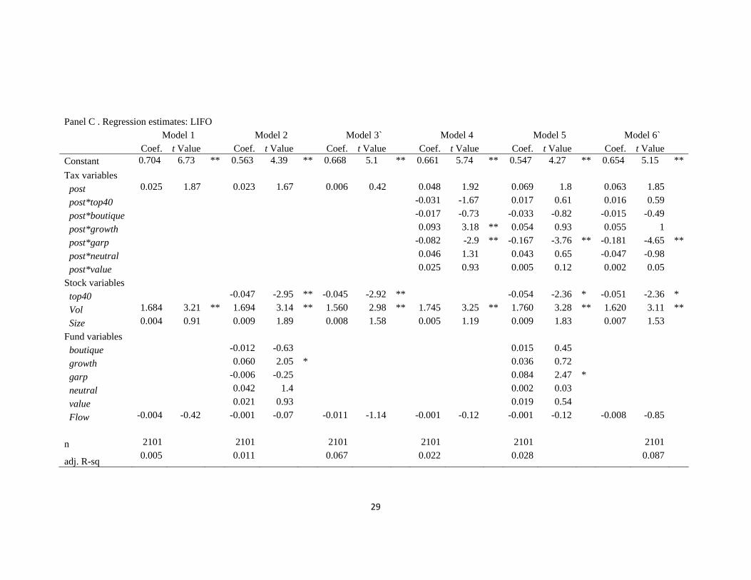
29
Panel C . Regression estimates: LIFO Model 1 Model 2 Model 3` Model 4 Model 5 Model 6` Coef. t Value Coef. t Value Coef. t Value Coef. t Value Coef. t Value Coef. t Value Constant 0.704 6.73 ** 0.563 4.39 ** 0.668 5.1 ** 0.661 5.74 ** 0.547 4.27 ** 0.654 5.15 ** Tax variables post 0.025 1.87 0.023 1.67 0.006 0.42 0.048 1.92 0.069 1.8 0.063 1.85 post*top40 -0.031 -1.67 0.017 0.61 0.016 0.59 post*boutique -0.017 -0.73 -0.033 -0.82 -0.015 -0.49 post*growth 0.093 3.18 ** 0.054 0.93 0.055 1 post*garp -0.082 -2.9 ** -0.167 -3.76 ** -0.181 -4.65 ** post*neutral 0.046 1.31 0.043 0.65 -0.047 -0.98 post*value 0.025 0.93 0.005 0.12 0.002 0.05 Stock variables top40 -0.047 -2.95 ** -0.045 -2.92 ** -0.054 -2.36 * -0.051 -2.36 * Vol 1.684 3.21 ** 1.694 3.14 ** 1.560 2.98 ** 1.745 3.25 ** 1.760 3.28 ** 1.620 3.11 ** Size 0.004 0.91 0.009 1.89 0.008 1.58 0.005 1.19 0.009 1.83 0.007 1.53 Fund variables boutique -0.012 -0.63 0.015 0.45 growth 0.060 2.05 * 0.036 0.72 garp -0.006 -0.25 0.084 2.47 * neutral 0.042 1.4 0.002 0.03 value 0.021 0.93 0.019 0.54 Flow -0.004 -0.42 -0.001 -0.07 -0.011 -1.14 -0.001 -0.12 -0.001 -0.12 -0.008 -0.85 n 2101 2101 2101 2101 2101 2101
adj. R-sq 0.005 0.011 0.067 0.022 0.028 0.087

30
` Coefficient estimates on fund_dummy(f)k not shown.
** Statistical significance at 1% probability or better.
* Statistical significance at 5% probability or better.
Panel D. Wald tests of coefficient estimates jointly equal to zero: LIFO Model 1 Model 2 Model 3 Model 4 Model 5 Model 6 Variables Chi-sq Chi-sq Chi-sq Chi-sq Chi-sq Chi-sq post 3.49 2.79 0.17 63.5 ** 45.7 ** 51.22 ** All tax variables 50.18 ** 41.27 ** 49.53 ** Stock variables 10.29 ** 18.32 ** 17.8 ** 10.71 ** 16.54 ** 15.49 ** Fund variables 0.18 9.38 423.94 ** 0.01 11.65 298.69 **