DIRECT-SEQUENCE SPREAD SPECTRUM SYSTEM DESIGNS FOR FUTURE
AVIATION DATA LINKS USING SPECTRAL OVERLAY
A Thesis Presented to
The Faculty of the
Fritz J. and Dolores H. Russ College of Engineering and Technology
Ohio University
In Partial Fulfillment
of the Requirement for the Degree
Master of Science
by
Joshua T. Neville
June, 2004

Acknowledgements
First, I would like to thank Dr. David Matolak for the help, guidance, and
opportunities he has provided. Without him, this work would have not been possible.
Next, I would like to thank my parents for giving me both the opportunity and
encouragement to pursue a higher education. Finally, I would like to thank my fhends
for their support.

Table of Contents
... ................................................................................ Acknowledgements ..ill
.................................................................................... Table of Contents iv
. . ........................................................................................ List of Tables vii
... ....................................................................................... List of Figures viii
............................................................................... Chapter 1 Introduction 1
............................................................................... 1.1Background 1
......................................................... 1.2 Aviation and Communication 2
................................................... 1.3 Direct-Sequence Spread-Spectrum 4
.............................................................................. 1.4 Thesis Scope 6
........................................................................... 1.5 Thesis Outline 7
...................................................... Chapter 2 Aviation Data Link Design Issues 8
....................................................................... 2.1 Setting and Model 8
.......................................... 2.2 Spectrum Availability in Potential Bands 14
......................................... 2.3 Aviation Data Link Traffic Characteristics 16
........................................ Chapter 3 DS-SS Overlay in the ILS Glide Slope Band 18
....................................................... 3.1 Introduction and Assumptions 18
............................................................ 3.2 Signals and System Model 20
.................................................... 3.3 Analysis of System Performance 23
.................................................................... 3.4 Numerical Results -27
....................................................... 3.5 ILS Performance Degradation 33
3.6 Multicarrier DS-SS ................................................................... -36
3.7 Summary ................................................................................ 39
Chapter 4 DS-SS Overlay in the MLS Band .................................................... 40
4.1 Introduction and Assumptions ....................................................... 40
4.2 Signals and System Model ............................................................ 41
4.3 Analysis of System Performance .................................................... 45
4.4 Multicarrier DS-SS .................................................................... 53
4.5 Numerical Results ...................................................................... 56
4.6 MLS Performance Degradation ...................................................... 63
4.7 Summary ............................................................................... -65
Chapter 5 System Comparisons ................................................................... 66
5.1 Introduction ............................................................................. 66
5.2 Center Frequency Considerations ................................................... 66
5.3 Bandwidth Considerations ............................................................ 69
5.4 Band Limited and Power Limited Channel ........................................ 71
........................ 5.5 Achievable Bit Rate, Number of Users, and Link Range 74
5.6 Conclusions ............................................................................. 90
............................................................ Chapter 6 Summary and Conclusions 92
6.1 Summary ................................................................................ 92
............................................................................. 6.2 Conclusions 93
6.3 Areas for Future Work ................................................................ 94
References ........................................................................................... -96

Appendix. . . . . . . . . . . . . . . . . . . . . . . . . . . . . . . . . . . . . . . . . . . . . . . . . . . . . . . . . . . . . . . . . . . . . . . . . . . . . . . . . . . . . . . . . . . . -98
Abstract.. . . . . . . . . . . . . . . . . . . . . . . . . . . . . . . . . . . . . . . . . . . . . . . . . . . . . . . . . . . . . . . . . . . . . . . . . . . . . . . . . . . . . . . . . . . .I24
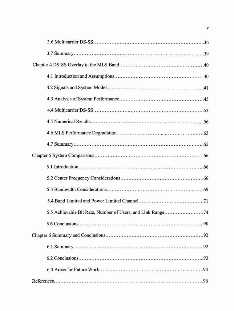
List of Tables
Table 4.1 MLS Signal Variance for Various Cases ............................................ 52
Table 5.1 Numerical evaluation parameter values used to generate Figure 5.3 ............. 76
Table 5.2 MU1 a Parameter Values and Corresponding Assumptions ....................... 82

List of Figures
Figure 1.1 Basic Block Diagram for a DCS ........................................................ 2
........................................... Figure 2.1 Single Signal Path or LOS Channel Model 9
Figure 2.2 The Power Spectral Density of Additive White Gaussian Noise (AWGN) ... 11
Figure 3.1 Illustration of power spectrum of ILS with SC-DS-SS overlay .................. 18
....................................................... Figure 3.2 DS-SS Overlay System Model 20
................................................... Figure 3.3 ILS Glide Slope Antenna Pattern 21
Figure 3.4 Block Diagram for a DS-SS Receiver ............................................... 24
Figure 3.5 DS-SS Pb vs . SNR (EdNo) with a processing gain of
................................................................. RJRb=SMHz15kbps=l 000 28
Figure 3.6 DS-SS Pb vs . SNR (EdNo) with a processing gain of
................................................................. RJRb=5MHz150kbps=l 00 29
Figure 3.7 Achievable DS-SS data rate Rb (bps) for given Pb vs . link range,
.......................................................................... in presence of ILS 30
Figure 3.8 Achievable DS-SS data rate Rb (bps) for given Pb vs . link range,
.............................................. in presence of ILS with PILS=PDS-SS+20 dB 31
Figure 3.9 Pb vs EdNO for DS-SS in presence of ILS; analytical and simulation
........................................................................................ results 33
Figure 3.10 ILS SNlR vs . DS-SS bandwidth; 3 ILS receiver bandwidths BILS.
........................................................................... ILS SNR=10 dB -34
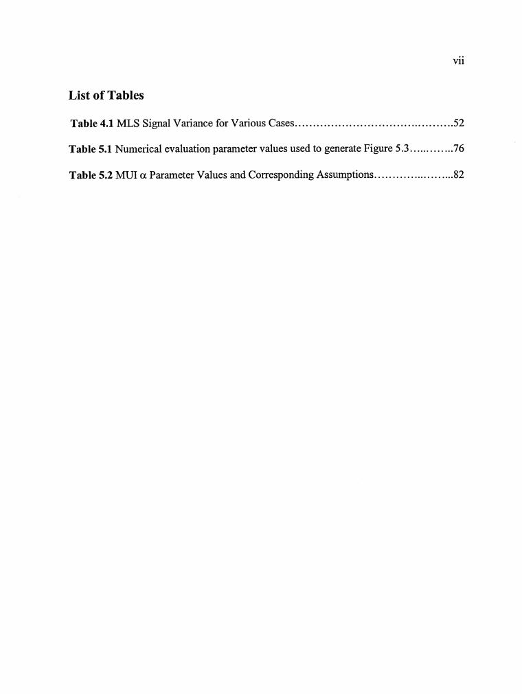
Figure 3.11 DS-SS Power Spectrum with Three ILS Receiver Filter Transfer
..................................................................................... Functions 35
....................................................... Figure 4.1 DS-SS Overlay System Model 41
Figure 4.2 Power Spectra of SC-DS-SS and MC-DS-SS Overlay in MLS band .......... 44
.............................................. Figure 4.3 Block Diagram for a DS-SS Receiver 45
Figure 4.4 Worst-case SC-DS-SS Pb vs . E& with various processing gains, data rates
.............................................................................. and JSR values 57
Figure 4.5 DS-SS Pb vs . EdNO with Rc=20 MHz, Rb=lOOkbps, 1 Mbps .................... 58
Figure 4.6 DS-SS Pb vs . EdNO with Rc=20 MHz. Rb=lOOkbps, 1 Mbps,
.................................................................................... Af-0 or R, 59
Figure 4.7 Achievable DS-SS data rate Rb (bps) for given Pb vs . link range,
....................................................................... in presence of MLS -61
Figure 4.8 Pb vs E& for DS-SS in presence of MLS; analytical and simulation
........................................................................................ results 62
.......................................... Figure 4.9 MLS Pb vs . E a o , for various JSR values 64
............................. Figure 5.1 Free Space Path Loss for ILS and MLS Frequencies 68
......... Figure 5.2 The Shannon-Hartley Capacity of the ILS and MLS Spectrum Bands 70
Figure 5.3 Achievable DS-SS Bit Rate Rb for a Single User in the ILS and MLS Bands
......................................... for Transmit Power levels of 10 and 30 Watts 74
Figure 5.4 Achievable DS-SS bit rate Rb (per user) versus the number of DS-SS users in
the ILS and MLS bands, with a transmit power of 10 Watts,
processing gains of 100 and 1200, and link distance of 5 km.. ...................... 77
Figure 5.5 Achievable DS-SS bit rate Rb (per user) in the ILS and MLS bands for
transmit power level of 10 Watts in the presence of MUI.. ........................... 79
Figure 5.6 Achievable DS-SS total bit rate versus the number of DS-SS users in the
ILS and MLS bands, with a transmit power of 10 Watts, processing gains of
100 and 1200, and link distance of 5 km.. .............................................. 83
Figure 5.7 Achievable DS-SS total bit rate versus the number of DS-SS users in the
ILS and MLS bands, with a transmit power of 10 Watts, processing gains of
......... 100 and 1200, MLS antenna gains of 10 dB, and link distance of 5 km.. .85
Figure 5.8 Achievable DS-SS bit rate Rb (per user) in the ILS and MLS bands for
transmit power level of 10 Watts in the presence of MU1 and antenna gains
...................................................................................... of 10 dB 87
Figure 5.9 Achievable DS-SS bit rate Rb (per user) in the ILS and MLS bands for
transmit power level of 10 Watts in the presence of equal MU1 and antenna
gains of 10 and 15 dB., ................................................................... 89

Chapter 1
Introduction
1.1 Background
Communication is the process of conveying information from one point to
another. Communication can occur through a large variety of media. Nowever, within
the scope of this thesis, communication will pertain to the transmission of information via
electrical means. The information comes from a source and is transmitted to a sink via a
path known as a channel. A channel may consist of space, wires, or wave-guides. Space
does not necessarily mean outer space. It can refer to earth's atmosphere. In this case,
we assume that the channel is earth's lower atmosphere. Information is transmitted
through the atmosphere using electromagnetic waves, that is to say wirelessly.
We also assume that the information transmitted across the aforementioned
channel is digital, that is to say discrete, in nature. By discrete, we mean that the
information may only take on certain values. For example, binary information may only
take one of two values. Binary information is commonly used in electronics where
components usually operate in one of two states. For instance, an electrical switch may
be on or off, but it cannot be partially on and partially off. The discrete nature of binary
circuits makes them more resilient against distortion andlor interference than an analog
circuit. This is because the distortion andlor interference must be so great as to shift the
digital circuit from one state to the other.
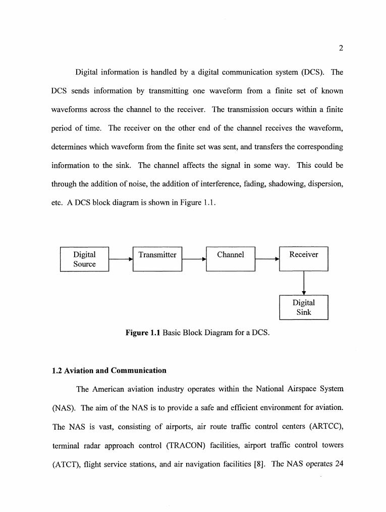
Digital information is handled by a digital communication system (DCS). The
DCS sends information by transmitting one waveform from a finite set of known
waveforms across the channel to the receiver. The transmission occurs within a finite
period of time. The receiver on the other end of the channel receives the waveform,
determines which waveform from the finite set was sent, and transfers the corresponding
information to the sink. The channel affects the signal in some way. This could be
through the addition of noise, the addition of interference, fading, shadowing, dispersion,
etc. A DCS block diagram is shown in Figure 1.1.
Figure 1.1 Basic Block Diagram for a DCS.
Digital Source
1.2 Aviation and Communication
The American aviation industry operates within the National Airspace System
(NAS). The aim of the NAS is to provide a safe and efficient environment for aviation.
The NAS is vast, consisting of airports, air route traffic control centers (ARTCC),
terminal radar approach control (TRACON) facilities, airport traffic control towers
(ATCT), flight service stations, and air navigation facilities [S]. The NAS operates 24
v Digital Sink
Transmitter Channel Receiver
hours a day and every day of the year. In addition, the NAS works with neighboring air
traffic control systems in order to support international flights [S].
The NAS ranks among the safest aviation systems in the world. However, the
NAS is aging and technologically behind other systems. Furthermore, the NAS is split
into several subsystems that cannot communicate with one another. This lack of
integration, in addition to the system's age and obsolescence, contribute to traffic
congestion, schedule delays, decreased operational predictability, and decreased
flexibility.
With these problems in mind, as well as the anticipated increase in aviation traffic
in the coming years, the Federal Aviation Administration (FAA) developed a
modernization plan for the NAS with input from the aviation community. This plan,
entitled NAS Architecture Version 4.0 [8], was approved in January 1999. The goals of
this plan included increases in safety, accessibility, flexibility, predictability, capacity,
efficiency, and security [S].
The plan also addresses NAS age and obsolescence. The age of the NAS makes
system upkeep expensive. One of the goals of the plan is to update the critical
infrastructure of the NAS in order to make the system more cost effective to operate and
maintain. Some examples of critical infrastructure include communication systems,
navigation systems, weather detection equipment, air traffic control computers and power
generation. In addition, another goal of the modernization plan is to provide new systems
with enhanced capabilities. Examples of these new systems include clear air-ground
communication via digital technology, precision-landing services for more locations via
satellite technology, and accurate weather data in the cockpit [8].
Communications are an essential part of the NAS. The NAS modernization plan
calls for replacing outdated hardware, integrating systems into a digital network, and
efficient use of the very high frequency (VHF) spectrum. The VHF band consists of
dedicated aeronautical spectrum from 1 18 MHz to 137 MHz. In reference to hardware,
the plan calls for the transition from analog radios to digital radios, a move that is
anticipated to increase VHF capacity by at least a factor of two [8].
One of the main components of the NAS communications architecture is
controller-pilot data link communications (CPDLC). CPDLC involves the exchange of
critical and non-critical data between pilots and controllers. An example of this data is
altimeter settings. The exchange of routine and repetitive messages via CPDLC serves to
reduce voice-channel congestion.
1.3 Direct-Sequence Spread-Spectrum
Spread-spectrum (SS) is the name given to communication techniques in which
information is transmitted using a bandwidth that is greater than the minimum bandwidth
required. In this way, it is bandwidth inefficient. However, SS has several benefits that
counter this drawback. These benefits include interference suppression, energy density
reduction, fine time resolution, and multiple access. In addition, security is a benefit that
comes from spread spectrum.
Two common forms of SS are direct-sequence spread-spectrum (DS-SS) and
frequency hopping spread-spectrum (FH-SS). In the case of DS-SS, the data signal is
multiplied by a unique, high rate spreading code that is independent of the data signal.
The spreading code is also known as a chipping code, and the bits of the spreading code
are called chips for clarity. At the DS-SS receiver, the received signal is correlated with a
copy of the spreading code, and the data signal is deciphered. This provides a measure of
security as well. Since the codes are unique, an unauthorized user would have difficulty
in trying to monitor communication between authorized users. When users of an SS
system are distinguished by such unique codes, this type of multiple access scheme is
called code division multiple access (CDMA).
In the case of FH-SS, the data signal is modulated via a narrowband signal with a
variable carrier frequency. This results in the data signal effectively hopping over a large
range of frequencies. The pattern of the hops is determined via a unique pseudorandom
noise (PN) sequence. FH-SS can operate over bandwidths on the order of several
gigahertz. Such bandwidths are an order of magnitude larger than those that can be
implemented in the case of DS-SS 191.
Several of the aforementioned benefits of SS can apply to aviation
communications. Interference suppression provides protection for critical
communications while reduced energy density for the DS-SS signal generates less
interference for other systems. Furthermore, CDMA provides security with unique
codes. It is relevant to note that the Global Positioning System (GPS) makes use of DS-
SSICDMA.
1.4 Thesis Scope
This research deals with the use of a DS-SS data link operating in spectral overlay
mode in either the Instrument Landing System (ILS) glide slope or the Microwave
Landing System (MLS) spectral bands. Spectral overlay means that the DS-SS data link
coexists with the respective landing system signal in the same spectral band at the same
time. Spectral overlay is something of a worst-case scenario in terms of system
performance. Orthogonal spectral allocations offer better system performance due to
reduced intersystem interference.
Classical analytical techniques are used to determine performance degradation, or
bit error rate (BER), experienced by the DS-SS signal in the presence of AWGN and
either the ILS glide slope signal or MLS signal. The performance degradation
experienced by the respective landing systems is also determined. This consists of
signal-to-noise-plus-interference-ratio (SNIR) for the ILS and both SNIR and BER for
the MLS. Using these analytical results, we generate example plots to predict DS-SS,
ILS, and MLS system performance. Computer simulations and numerical evaluations
were performed in MATLAB@ to corroborate the analytical results. In addition,
scenarios involving Multiple Carrier DS-SS (MC-DS-SS) were explored in both the ILS
glide slope and MLS bands, and these results are compared to those of the single-carrier
case.
1.5 Thesis Outline
The rest of the thesis is organized in the following manner. In Chapter 2, we
describe the signal and system model we used as well as the assumptions we made. In
Chapter 3, we derive analytical results for DS-SS spectral overlay in the ILS glide slope
band and plot both numerical and analytical results. Chapter 4 covers the derivation of
analytical results for DS-SS spectral overlay in the MLS band. The corresponding
numerical and analytical results are plotted as well. In Chapter 5, we compare the results
from Chapters 3 and 4. Chapter 6 consists of a summary of the thesis and touches on
areas for possible future work.
Chapter 2
Aviation Data Link Design Issues
2.1 Setting and Model
For any study that uses mathematical analysis of real physical systems, models
are required. The fidelity of the model can be critical to the validity of the results
obtained, but in general, the fidelity improves as the model complexity increases. We
generally compromise in both fidelity and complexity to satisfy the most important
constraints of interest. In our case, several of the models used are widely employed, and
broadly speaking, serve well to illustrate the dominant characteristics of the systems we
study.
The models and settings used in this work consisted of first order approximations
for the sake of analytical simplicity. The channel model consists of a single signal path,
or line of sight (LOS), between two transceivers, a ground station and an airborne station.
This is illustrated in Figure 2.1.

Direct
Figure 2.1 Single Signal Path or LOS Channel Model.
As mentioned previously, this model is a first order approximation. Thus, it does
not account for real world phenomena such as multipath signal propagation, signal
refraction, and fading. All of these phenomena are secondary when the elevation angle
between the aircraft and the ground station is large (e.g., greater than 15 degrees or so),
and under normal atmospheric conditions (e.g., no "ducting"). For low elevation angles
or in the presence of obstacles (man-made or natural), the single propagation path model
will not be valid, yet much of the work here can be extended to those more complicated
channels using known techniques [ l 11.
During propagation, it is assumed that the signal experiences free space path loss.
The fiee space path loss can be used to determine the signal's power as received by the
ground station when the airborne transmitter is located a known distance away and is
transmitting at a known frequency. Free space path loss L, is defined as follows [I].
Ls = ( 4 d / ~ y (2-1)
In (2-I), d is the distance between the transmitter and receiver, measured in
meters, and h is the wavelength of the signal in meters. The wavelength h can be
calculated from the frequency by
A = c / f (2-2)
where in (2-2), c is the speed of light in vacuum in meters per second and f is the
frequency of the transmitted signal in Hertz. Although propagation through the earth's
lower atmosphere will generally be at a velocity slightly lower than c, (2-2) is a very
good and widely used approximation.
The power of the signal received at the ground station from the airborne
transmitter can be calculated via
P, = EIRP/L, (2-3)
In (2-3), EIRP is the effective radiated power with respect to an isotropic radiator
measured in Watts, and L, is the free space path loss defined in (2-1). The EIRP is
defined as the product of the transmitted power and the gain of the transmitting antenna:
EIRP = P,G, (2-4)
where in (2-4), P, is the power of the transmitted signal in Watts, and Gt is the gain of the
transmitting antenna, which is dimensionless. The previous equations apply in the air to
ground (AG) transmission and the ground to air (GA) transmission cases.
The signal is assumed to be subject to additive white Gaussian noise (AWGN),
caused primarily by receiver front-end electronics. Spectral whiteness means that the
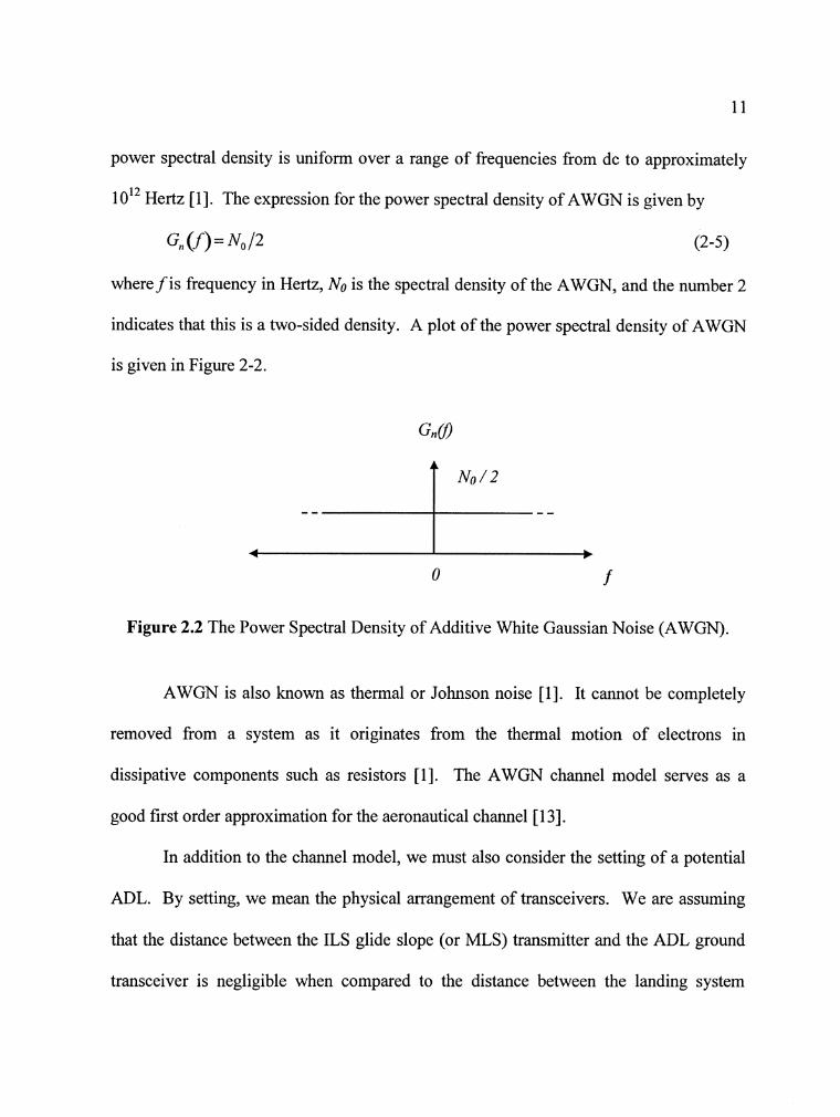
power spectral density is uniform over a range of frequencies from dc to approximately
1012 Hertz [I]. The expression for the power spectral density of AWGN is given by
Gn (f) = N,/2 (2-5)
where f is frequency in Hertz, No is the spectral density of the AWGN, and the number 2
indicates that this is a two-sided density. A plot of the power spectral density of AWGN
is given in Figure 2-2.
Figure 2.2 The Power Spectral Density of Additive White Gaussian Noise (AWGN).
AWGN is also known as thermal or Johnson noise [I]. It cannot be completely
removed from a system as it originates from the thermal motion of electrons in
dissipative components such as resistors [l]. The AWGN channel model serves as a
good first order approximation for the aeronautical channel [13].
In addition to the channel model, we must also consider the setting of a potential
ADL. By setting, we mean the physical arrangement of transceivers. We are assuming
that the distance between the ILS glide slope (or MLS) transmitter and the ADL ground
transceiver is negligible when compared to the distance between the landing system

transmitter and the transceiver on the aircraft. This distance between the aircraft and the
ADL transceiver on the ground is called the link range. The link itself is more complex.
It entails the entire path that information takes from source to sink. This path includes
encoding, modulation, transmission, the effects of the channel, reception, and processing
111.
The type of ADL link is also important to consider. We are interested in two-way
communication in both the AG and GA cases. However, we do not consider an ADL link
between two aircraft. This is would be an example of air-to-air (AA) communication.
Another aspect of a potential ADL is radio line-of-sight (RLOS). RLOS
determines whether two radios can "see" one another. RLOS can be affected by
obstacles such as physical topography, man-made objects, and the earth's horizon.
RLOS is important since it is possible to model the AG and GA radio links for a single
airport as a single cell belonging to a cellular system consisting of other airports. RLOS
can help determine whether there is interference from aircraft located in these outside
cells.
For VHF communications between an aircraft and a ground transceiver, this
RLOS must exist [14]. This is due to the rapid increase in attenuation experienced by the
signal when the link exceeds the RLOS [15]. RLOS is a function of altitude, but an
approximation can be used when RLOS values are much greater than aircraft altitudes
[15]. This approximation can be expressed for two antennas as
where re is the radius of the earth, hl is the altitude of the first antenna, h2 is the altitude
of the second antenna, and k is constant that accounts for refraction in the lower
atmosphere 1151. A typical value for k is 413 [15].
Finally, we must also consider the ADL link budget. The link budget determines
the amount of desired signal power and interference power that reaches the receiver.
These power levels help determine whether the communication system will operate with
the desired amount of error performance. A link budget can be complex, and an example
of such a budget is given in [I]. In our case, the link budget is less complex because this
is a first order study. For example, we can determine the ADL signal's received power
by the solving the following equation.
P r=P, -L ,+G,+Gr (2-7)
In (2-7), P, is the ADL received power in decibels, PI is the ADL transmit power in
decibels, L, is the free space path loss in decibels, GI is the gain of the transmitter antenna
in decibels, and G, is the gain of the receiver antenna in decibels.
Some of the interference at the receiver is due to AWGN, and we can determine
the power level of this noise via the following
P,, =-174+lOlogR, +NF (2-8)
In (2-8), P, is the noise power at the receiver in dBm, -174 dBrn/Hz is the value of
background noise measured in dBm per Hertz at a "room" temperature of 20" Celsius, Rb
is the bit rate of the ADL measured in bps, and NF is the noise figure of the ADL receiver
measured in dB. Additional interference comes from the ILS and MLS. Equations for
these sources of interference are developed in Chapters 3 and 4. In addition, the presence
of DS-SS multiple user interference (MUI) is considered in Chapter 5.
2.2 Spectrum Availability in Potential Bands
The current NAS architecture supports the operation of individual services and
users in separate frequency bands. Examples of such services consist of VHF
communications in the 1 18- 137 MHz frequency band and navigation in the 108-1 18
MHz, 330 MHz, and 900-1020 MHz frequency bands [2]. Specifically, we are interested
in the frequency bands reserved for the ILS glide slope and the MLS. The ILS glide
slope frequency band consists of the spectrum 329-335 MHz, and the MLS frequency
band consists of the spectrum 5031-5190.7 MHz [6]. One reason for our interest is that
both of these bands are currently reserved for aeronautical use. In addition, the ILS band
exhibits good propagation conditions, and the MLS band offers a combination of large
bandwidth and low use in the US [4].
In terms of spectrum availability, the ILS glide slope band offers approximately 5
MHz, as opposed to the approximately 160 MHz offered by the MLS band. However,
the ILS glide slope band offers better path loss when compared to that of the MLS band.
This difference in path loss can be quantified via (2-1). The higher path loss in the MLS
band can be offset via the use of directive antennas andlor higher transmit power, at the
expense of complexity, cost, and possibly coverage.
The difference in the amount of available spectrum between the ILS glide slope
and MLS bands affects several fundamental parameters that pertain to DS-SS
communication systems. One of these parameters is processing gain, which is defined in
the following equation [I].
GP = Rclrip /R*to (2-9)
In (2-9)' Rchip is the chip rate of a unique spreading code measured in chips per second,
and Rdala is the data rate measured in bits per second.
Processing gain serves as both a measure of a DS-SS system's protection against
interference and as a measure of the system's performance gain in terms of BER when
compared to a narrowband system. With a higher processing gain, the system's data is
spread over a larger bandwidth. At the receiver, when the desired data is despread with a
replica of the code, interference is spread by the same process. This spreading reduces
the power spectral density of the interference.
Spreading involves convolving spectra together. In the case of DS-SS, the data
signal is multiplied directly by the spreading code. Since Rchip is usually much greater
than Rdata, we can approximate the bandwidth of the spread signal by using Rchip.
However, if the chip and bit transitions are synchronous, Rchip is equal to the exact DS-SS
bandwidth and is no longer an approximation.
The MLS band offers a larger amount of spectrum over which to spread when
compared to that of the ILS glide slope band. This translates into a greater potential
processing gain for a fixed data rate. In addition, for a fixed value of processing gain, the
MLS band allows for a higher data rate than the ILS glide slope band. Indeed, for a large
available MLS bandwidth, both data rate and processing gain can be greater than that in
the ILS band.
2.3 Aviation Data Link Traffic Characteristics
Different aviation communication systems produce different traffic
characteristics. For instance, a theoretical ADL transceiver might produce a constant
flow of data from the ground to the ADL transceiver on the aircraft. This would be an
example of constant traffic. However, data traffic between an air traffic controller and a
pilot usually takes the form of verbal communication via a radio link. This traffic can be
thought of as having a burst like characteristic in that neither the pilot nor the controller is
continuously exchanging information. For example, a pilot may check with a controller
when entering that controller's airspace to confirm flight path information. Following
this exchange, the pilot and controller could possibly stop communicating until the pilot
leaves the airspace. Hence, there is a burst of traffic in the form of audible
communication followed by a long period of radio silence.
In terms of ADL design, traffic characteristics are important when considering
link capacity and access schemes. Certain access schemes tend to be more efficient when
carrying burst traffic as opposed to continuous traffic or vice-versa. For example, fixed-
assignment time-division-multiple-access (TDMA) is very efficient when traffic is heavy,
but it is wasteful when traffic is sporadic [I]. For analytical purposes, we assume
continuous signaling between the ADL transceivers. This is not necessarily a realistic
assumption, but it serves as a starting point for this first order study. The continuous case
can be altered to account for multiple users that are multiplexed andlor overlapping in
time by the inclusion of probability. Furthermore, transients in signaling are mostly of
interest in higher-layer operations, e.g. data link or media access control (MAC) layer.
Higher-layer operations refer to the International Standards Organizations (ISO) open
system interconnection (OSI) reference model. The OSI model is discussed in [12].
Chapter 3
DS-SS Overlay in the ILS Glide Slope Band
3.1 Introduction and Assumptions
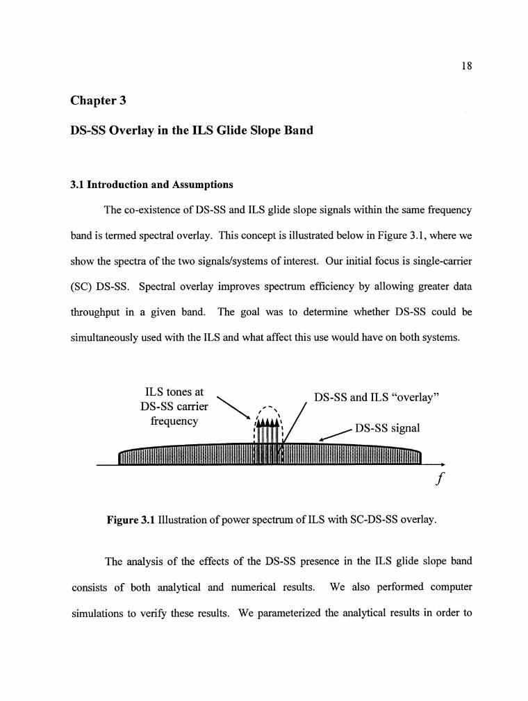
The co-existence of DS-SS and ILS glide slope signals within the same frequency
band is termed spectral overlay. This concept is illustrated below in Figure 3.1, where we
show the spectra of the two signals/systems of interest. Our initial focus is single-carrier
(SC) DS-SS. Spectral overlay improves spectrum efficiency by allowing greater data
throughput in a given band. The goal was to determine whether DS-SS could be
simultaneously used with the ILS and what affect this use would have on both systems.
ILS tones at DS-SS and ILS "overlay" DS-SS carrier
Figure 3.1 Illustration of power spectrum of ILS with SC-DS-SS overlay.
The analysis of the effects of the DS-SS presence in the ILS glide slope band
consists of both analytical and numerical results. We also performed computer
simulations to verify these results. We parameterized the analytical results in order to
examine the results over a wide range of system parameters. Examples of such
parameters include transmit power(s), and DS-SS data rate and chip rate. It is important
to note that ILS glide slope signal in Figure 3.1 is shown with 200 percent modulation.
Such modulation is rare in practice, but it can be done.
Some assumptions were made in the analysis. To begin with, we assumed the ILS
glide slope signal was centered on the carrier frequency of the DS-SS signal. This is the
worst-case scenario for both DS-SS performance and the ILS glide slope. In addition, we
assumed the distance between the ILS glide slope transmitter and the DS-SS transceiver
was negligible when compared to the distance between the aircraft and the ILS glide
slope transmitter and DS-SS transceiver; that is, the ILS and DS-SS ground stations are
close in comparison to the AG link range. In addition, the effects of multipath
propagation were ignored in order to simplify the analysis. This is a reasonable
assumption for a first order analysis because there will usually be a LOS between the
aircraft and the ILS glide slope transmitter and DS-SS transceiver. In addition, the major
multipath contribution may be from ground reflections, and the delay difference between
this reflection and the LOS signal will be negligible in comparison to the DS-SS symbol
time. Given these conditions, we used an AWGN model for the channel. Finally, we
assumed coherent detection in order to further simplify analysis.

3.2 Signals and System Model
A block diagram of the system model can be seen in Figure 3.2.
Figure 3.2 DS-SS Overlay System Model.
DS-SS TX
The ILS uses amplitude modulation (AM). The DS-SS receiver sees the glide
slope signal in the form as defined in (3-1). For clarity, any mention of the ILS or ILS
signal refers to the ILS glide slope unless otherwise noted.
g(t) = A, [I+ k,m(tllcos(2~~t) (3-1)
In (3-I), A, is the amplitude of the received signal, k, is the amplitude modulator
constant, f, is the carrier frequency (329-335 MHz), and m(t) is the message signal. As
previously mentioned, the worst-case scenario in terms of DS-SS performance is when
the center frequency of the ILS signal is equal to the DS-SS carrier frequency. We
analyzed this case first. The message signal m(t) is defined in (3-2).
C ' ' ILS &
DS-SS Rx's

m(t) = A' cos(2ii150t) + A' cos(2n90t) (3 -2)
In (3-2), A' is the amplitude of the tones at 150 and 90 Hz from the carrier. We assumed
that the amplitude of the tones were equal [6].
The glide slope signal g(t) can be expanded via trigonometric identities.
In (3-3), f,+90 = f, + 90 Hz, f,-90 = f, - 90 Hz, and likewise for the 150 Hz tones. The
antenna pattern of the ILS glide slope signal is shown in Figure 3.3. Figure 3.3 was
inspired by [6].
Glide Slope (0 = 3 deg.)
0 Relative Field Strength (%) 100
Figure 3.3 ILS Glide Slope Antenna Pattern.
When an aircraft is above the glide slope, the 90 Hz tone dominates [6]. In this
case, the vertical deviation indicator (VDI) needle reads "fly down" [6]. When the
aircraft is below the glide slope, the 150 Hz tone dominates. In this case, the VDI needle
reads "fly up" [6].
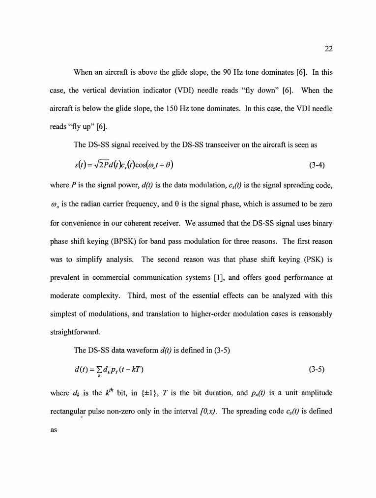
The DS-SS signal received by the DS-SS transceiver on the aircraft is seen as
~ ( t ) = ~ d ( t ) r s ( t ) c o s ( w 0 t + e) (3 -4)
where P is the signal power, d(t) is the data modulation, c,(t) is the signal spreading code,
w, is the radian carrier frequency, and 8 is the signal phase, which is assumed to be zero
for convenience in our coherent receiver. We assumed that the DS-SS signal uses binary
phase shift keying (BPSK) for band pass modulation for three reasons. The first reason
was to simplify analysis. The second reason was that phase shift keying (PSK) is
prevalent in commercial communication systems [I], and offers good performance at
moderate complexity. Third, most of the essential effects can be analyzed with this
simplest of modulations, and translation to higher-order modulation cases is reasonably
straightforward.
The DS-SS data waveform d(t) is defined in (3-5)
where dk is the Ph bit, in {&I), T is the bit duration, and p,(t) is a unit amplitude
rectangular pulse non-zero only in the interval [O,x). The spreading code c,(t) is defined
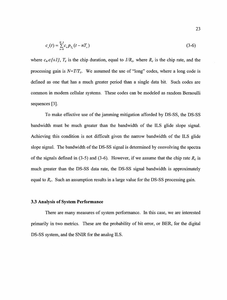
where c~E{*~), TC is the chip duration, equal to l / R , where Rc is the chip rate, and the
processing gain is N=T/T,. We assumed the use of "long" codes, where a long code is
defined as one that has a much greater period than a single data bit. Such codes are
common in modern cellular systems. These codes can be modeled as random Bernoulli
sequences [3].
To make effective use of the jamming mitigation afforded by DS-SS, the DS-SS
bandwidth must be much greater than the bandwidth of the ILS glide slope signal.
Achieving this condition is not difficult given the narrow bandwidth of the ILS glide
slope signal. The bandwidth of the DS-SS signal is determined by convolving the spectra
of the signals defined in (3-5) and (3-6). However, if we assume that the chip rate R, is
much greater than the DS-SS data rate, the DS-SS signal bandwidth is approximately
equal to Rc. Such an assumption results in a large value for the DS-SS processing gain.
3.3 Analysis of System Performance
There are many measures of system performance. In this case, we are interested
primarily in two metrics. These are the probability of bit error, or BER, for the digital
DS-SS system, and the SNIR for the analog ILS.
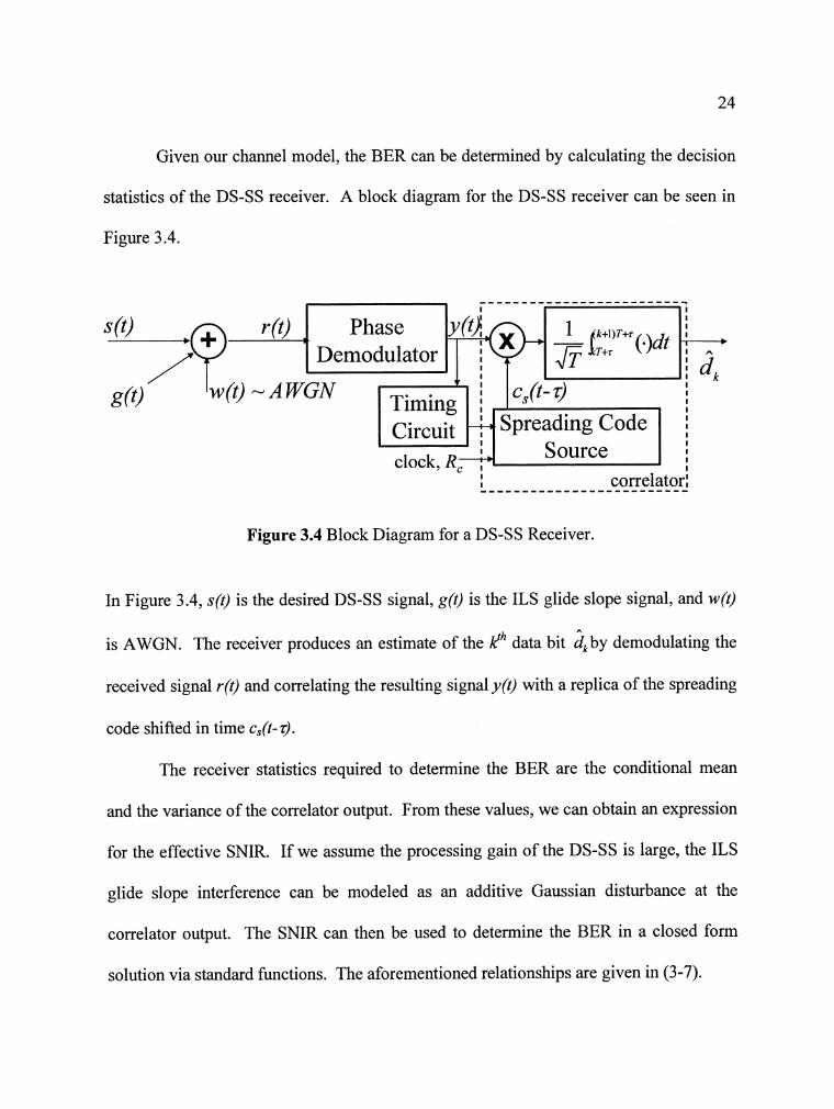
Given our channel model, the BER can be determined by calculating the decision
statistics of the DS-SS receiver. A block diagram for the DS-SS receiver can be seen in
Figure 3.4.
.. I I correlatorl . . . . . . . . . . . . . . . . . . . . . . . . .
rft) ,.
Figure 3.4 Block Diagram for a DS-SS Receiver.
. . . . . . . . . . . . . . . . . . . . . . . . . I I
Phase Demodulator
I
In Figure 3.4, s(t) is the desired DS-SS signal, g(t) is the ILS glide slope signal, and w(t)
is AWGN. The receiver produces an estimate of the gh data bit i kby demodulating the
received signal r(t) and correlating the resulting signal y(t) with a replica of the spreading
code shifted in time c,(t- 4.
The receiver statistics required to determine the BER are the conditional mean
and the variance of the correlator output. From these values, we can obtain an expression
for the effective SNIR. If we assume the processing gain of the DS-SS is large, the ILS
glide slope interference can be modeled as an additive Gaussian disturbance at the
correlator output. The SNIR can then be used to determine the BER in a closed form
solution via standard functions. The aforementioned relationships are given in (3-7).
I - AWGN ' i c,(t-.r) I
Timing : I I I
Spreading Code : Circuit T I
I Source clock, R,-
I I I
In (3-7), S is the square of the mean value of the conelator output d, given dk=+l sent, N
is the variance of the AWGN component, and I is the variance of ILS glide slope signal
component. The Q-function is defined as Q(x) = re-"" /&, and it represents the tail
integral of a zero mean, unit variance Gaussian probability density function.
In AWGN with no interference, the performance of DS-SS with BPSK
modulation is equal to that of un-spread coherent BPSK in AWGN [3]. This BER
expression is shown in (3-8) [3].
BER = P, = ~(m)= Q [El In (3-8), Eb is the received bit energy and No is the one-sided noise power spectral
density.
In order to account for the presence of the ILS glide slope signal, (3-8) must be
modified. This modification is accomplished by "feeding" the ILS glide slope signal
through the DS-SS receiver in Figure 3.4 and calculating the variance of the resulting
output from the correlator.
The first step in calculating the variance involves down converting the received
ILS signal and filtering out the double frequency components. The result of the down
converting and filtering is shown in (3-9).

In (3-9), we have redefined the ILS glide slope signal to be I(t) instead of g(0, which is
shown in Figure 3.4. This change is meant to convey the notion that the ILS is
considered interference from the perspective of the DS-SS receiver. Following the down
conversion, the signal in (3-9) is multiplied by the spreading code c,(t-4; we assume that
z is equal to zero without loss of generality. This results in the ILS part of the estimate
within &, which is shown in (3- 10).
In (3-lo), A"=ACAJkd2 and the other variables are equal to those previously defined. If
we assume that the mean value of the spreading code is equal to zero, then the mean
value of (3-10) is also equal to zero. The variance of (3-10) can then be calculated by
finding the mean value of the square of (3-10). The resulting expression for the variance
is shown in (3- 1 1).
+ y[2ay cos(ir90Tc (2n + 1)) + y2 cos2 ( ~ 9 0 ~ ~ (2n + l))] (3-1 1) n=O
In (3-ll), a=AcTJ2, ,0=cwsin(x150Tc)/(ii150Tc), and y= asin(n90Tc)/(n90Tc). With
(3-1 I), we can obtain the BER expression for DS-SSIBPSK in the presence of the ILS
glide slope signal. This expression is shown in (3-12).
BER = Q(/r] No + 40: /T
In (3-12), Eb is the received DS-SS bit energy, No is the power spectral density of
AWGN, 0; is the variance of the ILS signal, and T is the DS-SS bit period.
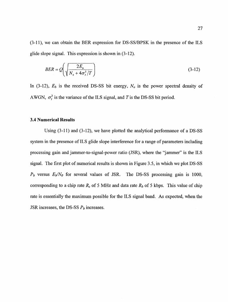
3.4 Numerical Results
Using (3-1 1) and (3-12), we have plotted the analytical performance of a DS-SS
system in the presence of ILS glide slope interference for a range of parameters including
processing gain and jammer-to-signal-power ratio (JSR), where the "jammer" is the ILS
signal. The first plot of numerical results is shown in Figure 3.5, in which we plot DS-SS
Pb versus EdNo for several values of JSR. The DS-SS processing gain is 1000,
corresponding to a chip rate R, of 5 MHz and data rate Rb of 5 kbps. This value of chip
rate is essentially the maximum possible for the ILS signal band. As expected, when the
JSR increases, the DS-SS Pb increases.
0 5 10 15 20 25 SNR (dB)
Figure 3.5 DS-SS Pb VS. SNR (EdNo) with a processing gain of RJRb=5MHz15kbps=l 000.
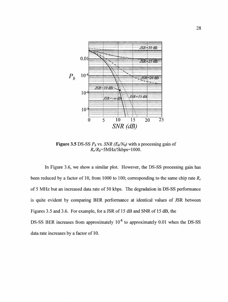
In Figure 3.6, we show a similar plot. However, the DS-SS processing gain has
been reduced by a factor of 10, from 1000 to 100; corresponding to the same chip rate R,
of 5 MHz but an increased data rate of 50 kbps. The degradation in DS-SS performance
is quite evident by comparing BER performance at identical values of JSR between
Figures 3.5 and 3.6. For example, for a JSR of 15 dB and SNR of 15 dB, the
DS-SS BER increases from approximately lo-* to approximately 0.01 when the DS-SS
data rate increases by a factor of 10.
SNR (dB)
Figure 3.6 DS-SS Pb VS. SNR (EdNo) with a processing gain of RJRb=5MHz150kbps=1 00.
We are also interested in obtaining estimates of the achievable bit rate for the DS-
SS system in the presence of the ILS glide slope signal. The following results were
obtained numerically. The procedure consists of setting up a simple link budget
equation, assuming values for certain parameters, and then solving for the data rate. We
assumed that both the ILS and DS-SS transmitters transmitted 1 Watt of power, all
antenna gains were 0 dB, and the DS-SS receiver noise figure was 10 dB. The path loss
was modeled as that of free space, and a chip rate of 5 MHz was assumed for the DS-SS
system. Furthermore, we assumed the distance between the DS-SS and ILS transmitters
was negligible when compared to the distance between the aircraft and the runway, e.g.
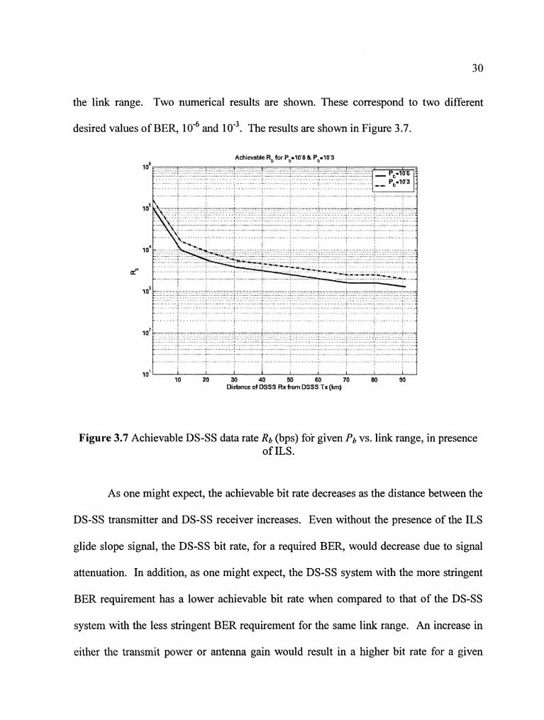
the link range. Two numerical results are shown. These correspond to two different
desired values of BER, and The results are shown in Figure 3.7.
Achievable Rb for Pb.10'6 6. P,.10'3
10 20 30 40 Distance of DSSS Rx from DSSS Tx (km)
Figure 3.7 Achievable DS-SS data rate Rb (bps) for given Pb VS. link range, in presence of ILS.
As one might expect, the achievable bit rate decreases as the distance between the
DS-SS transmitter and DS-SS receiver increases. Even without the presence of the ILS
glide slope signal, the DS-SS bit rate, for a required BER, would decrease due to signal
attenuation. In addition, as one might expect, the DS-SS system with the more stringent
BER requirement has a lower achievable bit rate when compared to that of the DS-SS
system with the less stringent BER requirement for the same link range. An increase in
either the transmit power or antenna gain would result in a higher bit rate for a given
BER. Finally, it is important to note these results were obtained for un-coded
modulation. The use of forward error correction (FEC) would result in lower BER values
andlor larger data rates.
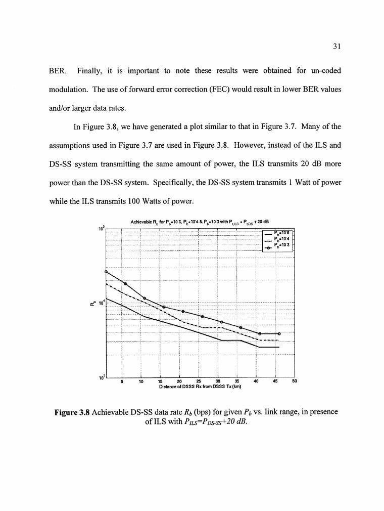
In Figure 3.8, we have generated a plot similar to that in Figure 3.7. Many of the
assumptions used in Figure 3.7 are used in Figure 3.8. However, instead of the ILS and
DS-SS system transmitting the same amount of power, the ILS transmits 20 dB more
power than the DS-SS system. Specifically, the DS-SS system transmits 1 Watt of power
while the ILS transmits 100 Watts of power.
Figure 3.8 Achievable DS-SS data rate Rb (bps) for given Pb VS. link range, in presence of ILS with P I L ~ = P ~ ~ - ~ ~ + ~ ~ dB.
Achtevable R,, for Pb*10 6, Pb.104 & P,.-103 wtth P ,,[, = P ,,nS t 20 dB
l o 5 . t I I I I - Pb-10 6 .- C - A - 3 P,mlO-4 ...
-$- P,-103 -
l o 3 - I I I I I a I f I
5 10 15 20 25 30 35 40 45 50 D~stance of DSSS Rx from DSSS Tx (km)

The plots in Figure 3.8 represent a more realistic scenario for a DS-SS ADL. As
expected, the DS-SS bit rate is reduced when the ILS transmits more power. For
example, at a link distance of 5 kilometers, for equal ILS and DS-SS transmit powers and
a required BER of the DS-SS bit rate is approximately 13 kbps. If the ILS transmits
20 dB more power, the DS-SS bit rate drops to approximately 9 kbps. However, as the
link range increases, the difference in DS-SS bit rate between the equal and unequal
transmit power cases decreases. For example, at a link distance of 45 kilometers, for
equal ILS and DS-SS transmit powers and a required BER of the DS-SS bit rate is
approximately 3 kbps. If the ILS transmits 20 dB more power, the DS-SS bit rate drops
to approximately 2.5 kbps. As the link distance increases, both the DS-SS signal and ILS
interference undergo greater attenuation due to path loss. As a result, the effect of path
loss on the DS-SS bit rate is much greater than the effect of ILS interference when the
link distance is large.
In Figure 3.9, we have plotted the analytical results for DS-SS BER performance
in the presence of the ILS glide slope signal and AWGN as a function of E& (3-12)
along with simulation results obtained in MATLAD@. The simulation was performed in
order to corroborate the analytical results. The resulting agreement is excellent.

Pb vs EbMD for DSSS BPSK on AWGN Channel
4, Pbd-Multi-Tone Jammed at fc.S~mulated (JIS) = 9 dB
Figure 3.9 Pb VS. EdNO for DS-SS in presence of ILS; analytical and simulation results.
3.5 ILS Performance Degradation
An important concern that we have not yet addressed is the degradation of the ILS
glide slope signal by the DS-SS signal. The analysis of this degradation is somewhat less
complicated than that given in the previous section, e.g. DS-SS degradation in the
presence of the ILS glide slope signal. This is because the interference due to the DS-SS
signal can be modeled as additional AWGN. The presence of the DS-SS signal will
reduce the effective SNR for the ILS signal. This can be illustrated by the following:
SNR = S,, / N > SNIR = S, /(N + I,,) (3-13)
In (3-13), SILS is the received ILS glide slope signal power, N is the power spectral
density of the background noise, and IDS is the DS-SS signal power within the ILS
receiver bandwidth. The value for IDS can be approximated by (3-14).
IDS ~(BILS / R c ) (3-14)
In (3-14), P is the DS-SS received signal power, BILs is the bandwidth of the ILS glide
slope receiver, and R, is the chip rate of the DS-SS signal. The approximations generated
via (3-13) and (3-14) should be very good if the DS-SS chip rate is much greater than the
ILS bandwidth, and the ILS receiver filter roll-off is good, that is to say steep.
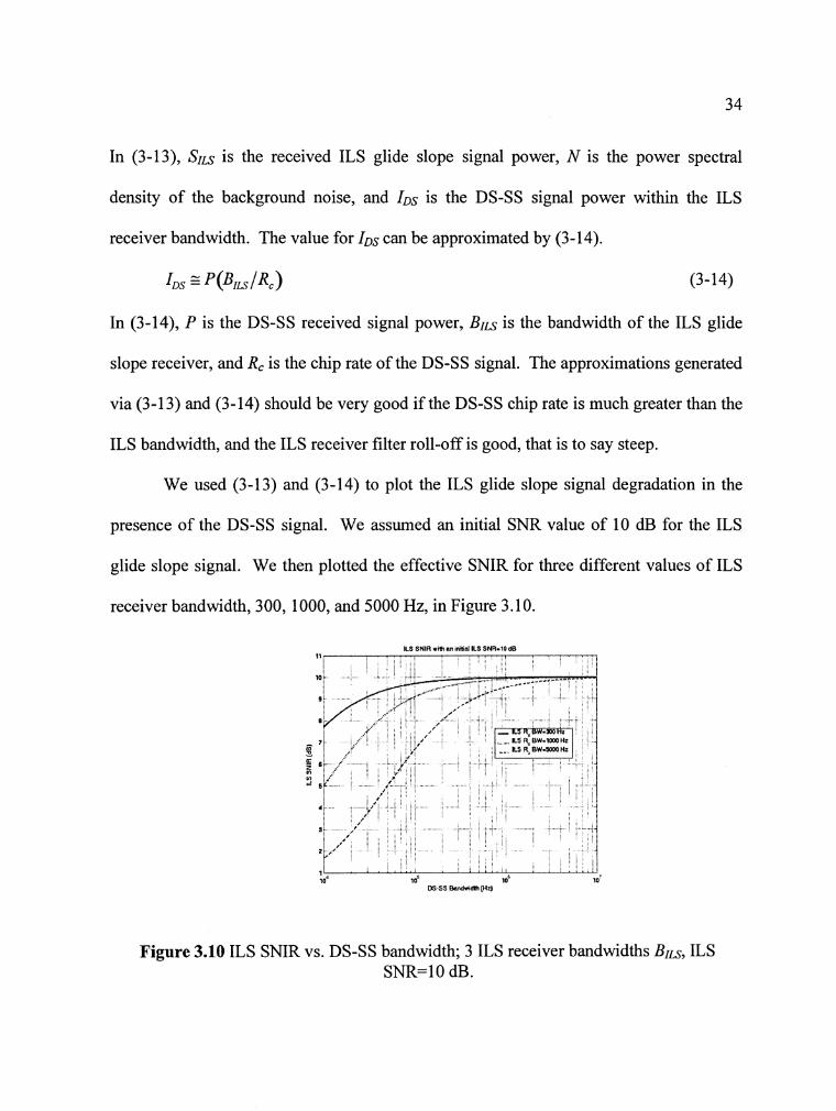
We used (3-13) and (3-14) to plot the ILS glide slope signal degradation in the
presence of the DS-SS signal. We assumed an initial SNR value of 10 dB for the ILS
glide slope signal. We then plotted the effective SNIR for three different values of ILS
receiver bandwidth, 300, 1000, and 5000 Hz, in Figure 3.10.
ILS SNIR vim nntniaai 11s SNR-10dB
Figure 3.10 ILS SNIR vs. DS-SS bandwidth; 3 ILS receiver bandwidths BILs, ILS SNR=10 dB.
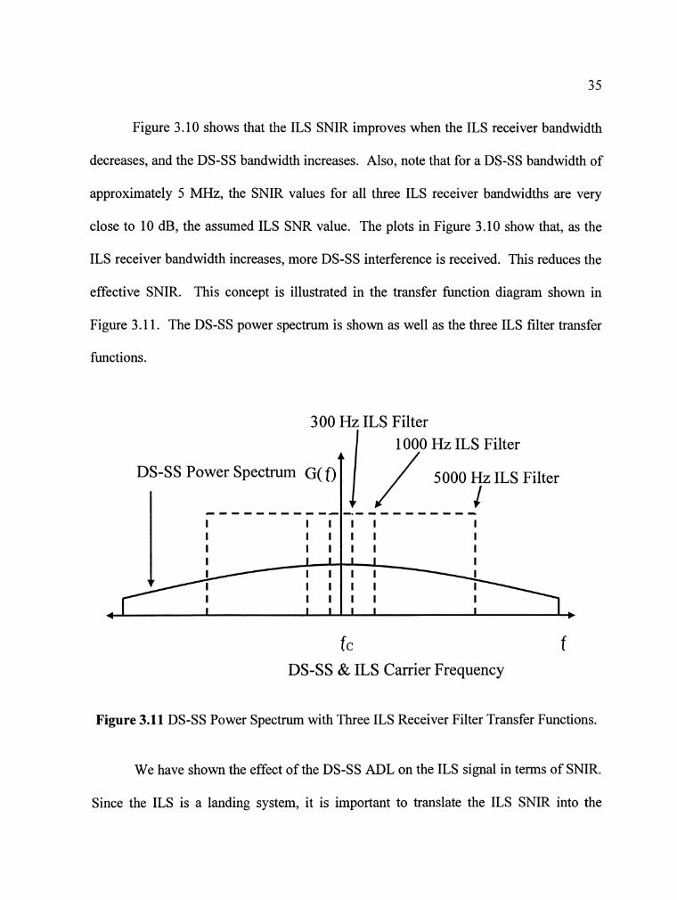
Figure 3.10 shows that the ILS SNIR improves when the ILS receiver bandwidth
decreases, and the DS-SS bandwidth increases. Also, note that for a DS-SS bandwidth of
approximately 5 MHz, the SNIR values for all three ILS receiver bandwidths are very
close to 10 dB, the assumed ILS SNR value. The plots in Figure 3.10 show that, as the
ILS receiver bandwidth increases, more DS-SS interference is received. This reduces the
effective SNIR. This concept is illustrated in the transfer function diagram shown in
Figure 3.11. The DS-SS power spectrum is shown as well as the three ILS filter transfer
functions.
300 Hz ILS Filter 1000 Hz ILS Filter
DS-SS Power Spectrum G(f ) 5000 Hz ILS Filter
I 1 1 1 1
1 - - - - - - - - - - - - . - - - - - - - - - - I
I 1 1 1 1 I I 1 1 1 1 I i I I 1 1 1 1 I I 1 1 1 1 I I 1 1 1 1 I
4 b
fc f DS-SS & ILS Carrier Frequency
Figure 3.11 DS-SS Power Spectrum with Three ILS Receiver Filter Transfer Functions.
We have shown the effect of the DS-SS ADL on the ILS signal in terms of SNIR.
Since the ILS is a landing system, it is important to translate the ILS SNIR into the
equivalent position error. This translation would give a better idea of the effect the DS-
SS ADL would have on ILS operation. Such a translation is left for future work.
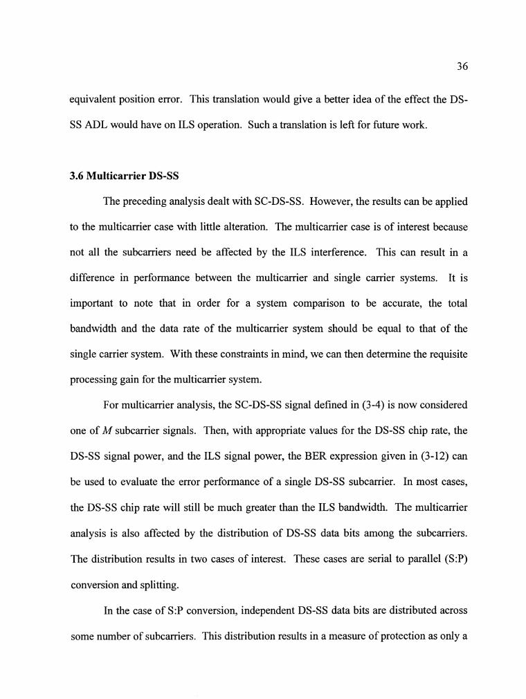
3.6 Multicarrier DS-SS
The preceding analysis dealt with SC-DS-SS. However, the results can be applied
to the multicarrier case with little alteration. The multicarrier case is of interest because
not all the subcarriers need be affected by the ILS interference. This can result in a
difference in performance between the multicarrier and single carrier systems. It is
important to note that in order for a system comparison to be accurate, the total
bandwidth and the data rate of the multicarrier system should be equal to that of the
single carrier system. With these constraints in mind, we can then determine the requisite
processing gain for the multicarrier system.
For multicarrier analysis, the SC-DS-SS signal defined in (3-4) is now considered
one of M subcarrier signals. Then, with appropriate values for the DS-SS chip rate, the
DS-SS signal power, and the ILS signal power, the BER expression given in (3-12) can
be used to evaluate the error performance of a single DS-SS subcarrier. In most cases,
the DS-SS chip rate will still be much greater than the ILS bandwidth. The multicarrier
analysis is also affected by the distribution of DS-SS data bits among the subcarriers.
The distribution results in two cases of interest. These cases are serial to parallel (S:P)
conversion and splitting.
In the case of S:P conversion, independent DS-SS data bits are distributed across
some number of subcarriers. This distribution results in a measure of protection as only a
fraction of the bits will generally be affected by the ILS interference. For the S:P case,
the symbol rate R, for a subcarrier is
where Rb is the input DS-SS bit rate, and M is the number of subcarriers over which the
data bits are distributed. The energy of each subcarrier symbol is equal to the DS-SS bit
energy Eb. This distribution results in one of every M bits being affected by the ILS
interference, when the ILS spectrum spans only a single subcarrier.
The BER for S:P conversion is found by calculating the average BER over the M
subcarriers. Assuming only one subcarrier incurs ILS interference, the resulting BER
expression is
In (3-16), PbA is the performance of the modulation in AWGN, and Pbl is the performance
in the presence of the ILS interference. For BPSK in AWGN with no interference, the
BER is given by (3-8). For BPSK in AWGN with ILS interference, the BER is given by
(3-12). The processing gain of the multicarrier and single carrier systems can be shown
to be equal via (3 - 17).
In the second MC case of splitting, the energy of each DS-SS data bit is
distributed among M subcarriers. With this distribution, every data bit is affected by ILS

interference, but only l/Adh of the bit energy is "lost". The bit energy for the ith
subcarrier Ebi is defined as
and the bit rate for the ith subcarrier Rsi is equal to the single carrier bit rate Rb. The
DS-SS receiver has M correlators, and the sum of these M correlators is then used to
make a bit decision via maximal ratio combining.
The BER for splitting is found by taking the mean and variance of the
aforementioned correlator sum. The mean of each correlator output is Jm. The
mean of the sum of M such correlators is Jm. The variance is equal to the sum of
the noise variances on each subcarrier. This is equal to 4-. The resulting
BER expression for splitting is shown in (3-1 9).
In this case, the multicarrier processing gain NIMC2 is equal to the processing gain
of the single carrier divided by the number of subcarriers. This relationship is illustrated
in (3-20).
In (3-20), Rc,MCZ is the chip rate of the multicarrier system, Rs,MCZ is the symbol rate of the
multicarrier system, R,sc is the chip rate of the single carrier system, Nsc is the

processing gain of the single carrier system, M is the number of subcarriers, and Rb is the
DS-SS bit rate.
3.7 Summary
We have examined the feasibility of DS-SS spectral overlay in the ILS glide slope
band. Feasibility is dependent upon the DS-SS BER and the ILS SNIR. A potential
ADL must possess a satisfactory BER while not degrading ILS SNIR to the point that the
landing system fails to meet FAA specifications. Using classical analytical techniques
and a first order channel model, we obtained an expression for the BER performance of
DS-SS in the presence of the ILS glide slope signal. This BER expression was
corroborated with computer simulations. Due to the parametric nature of the equations,
results were plotted for a number of different system parameters. The main DS-SS
parameters of interest were the processing gain and chip rate. The main ILS parameter of
interest was the SNIR. The attainable SNIR of the ILS glide slope signal in the presence
of the DS-SS signal was also provided. The results that were obtained indicate that
spectral overlay of DS-SS in the ILS glide slope band is feasible given a slight
degradation in ILS SNR or a slight reduction in ILS range.

Chapter 4
DS-SS Overlay in the MLS Band
4.1 Introduction and Assumptions
The concept of DS-SS spectral overlay can also be applied to the MLS band. The
analysis for the MLS band is similar to the treatment for the ILS band found in the
previous chapter. The main difference between the two analyses lies in the different
signal format and modulation employed by the MLS. This results in a longer and more
complex analysis.
Some of the assumptions from the previous chapter are carried over. We assumed
that the MLS carrier frequency was centered on the DS-SS carrier frequency. This is the
worst-case scenario in terms of DS-SS performance. However, we also examined cases
when the carrier frequencies were not centered on one another. In addition, we assumed
the distance between the DS-SS and MLS ground stations is negligible when compared to
the distance between the ground stations and the transceiver on board the aircraft, e.g. the
link range. The effects of inultipath are again ignored in order to simplify analysis. As
mentioned in the previous chapter, this is a reasonable assumption for a first order
analysis as there will usually be a line of sight between the respective ground stations and
the aircraft. With these conditions, an AWGN channel model was used. Coherent
detection was assumed to simplify the analysis. Additional assumptions are noted.
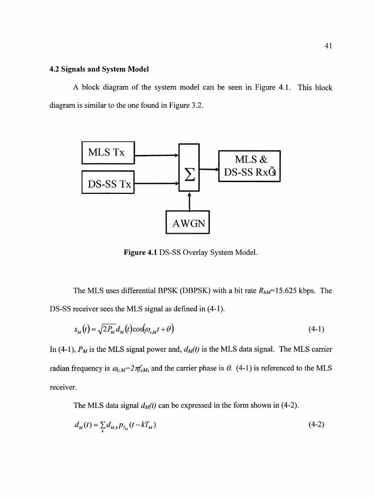
4.2 Signals and System Model
A block diagram of the system model can be seen in Figure 4.1. This block
diagram is similar to the one found in Figure 3.2.
Figure 4.1 DS-SS Overlay System Model.
MLS Tx
DS-SS TX
The MLS uses differential BPSK (DBPSK) with a bit rate Rbp15.625 kbps. The
DS-SS receiver sees the MLS signal as defined in (4-1).
s, ( t) = a d M ( t ) c o ~ ( % ~ t + 8) (4-1)
In (4-I), PM is the MLS signal power and, dM(' is the MLS data signal. The MLS carrier
radian frequency is ~ ~ , ~ = 2 $ ~ ~ , and the carrier phase is 8. (4-1) is referenced to the MLS
receiver.
The MLS data signal dM(g can be expressed in the form shown in (4-2).
d,u (t) = CdM,k P , (t - kT, ) k
(4-2)
9
* x. ' MLS &
DS-SS R X ~
In (4-2), d M k ~ {rtl) is the Ph MLS data bit, TM=I/RbM is the MLS bit duration, andp,(t) is
a unit amplitude rectangular pulse non-zero only in the interval [O,x).
As mentioned previously, the MLS uses DBPSK. The Ph MLS information bit
bke {O,1) is related to dMx by dMk=2(r7,,,-, Qb6J-I. The variable zM7,,, is the logical binary
- version of dMk, i.e., dMli-, E {O,l), and dMk=2&,-I, and the symbol 8 is the logical
exclusive-OR [I] [6].
The basic MLS setup consists of azimuth and elevation ground stations and
distance measuring equipment (DME) [6]. This setup can be expanded to include a back-
azimuth station that can be used for departure guidance andlor missed approaches [6].
The ground stations transmit angle and data messages along the line of the runway [6].
Angle messages consist of azimuth and elevation information while the data message
consists of eight basic data words [6].
The MLS antennas employ a narrow beam width. For elevation, a vertical-pattern
beam width of 2 degrees or less is required to avoid undesired ground reflection [6]. The
elevation beam scans from an elevation that is slightly below horizontal to a typical
elevation of 15 degrees [6]. For azimuth, a lateral-pattern beam width of 2 degrees can
meet requirements for runways less than 8,000 feet long [6]. Runways longer than 8,000
feet require a lateral-pattern beam width of 1 degree [6]. These narrow beam widths
suppress undesired reflections from lateral reflections such as hangers [6]. The azimuth
beam scans back and forth across the runway, from 40 degrees left of the center to 40
degrees right of center [6]. This results in an 80 degree scan sector [6].
The single carrier (SC) DS-SS signal received by the DS-SS receiver on the
aircraft was defined in (3-4). That definition is restated in a slightly different form and
shown in equation (4-3).
s(t) = m d ( t ) ~ ( t ) c o s ( ~ t + eS) (4-3)
In (4-3), P is the received DS-SS signal power, d(t) is the data modulation, c(t) is the
signal spreading code, @,is the radian carrier frequency, and 8, is the signal phase, which
is assumed to be zero for convenience in our coherent receiver. We assumed that the
DS-SS signal used BPSK for band pass modulation for two reasons. The first was to
simplify analysis. The second was that PSK is prevalent in commercial communication
systems [I]. The DS-SS data waveform d(t) was defined in (3-5). That definition is
restated here:
d(t) = C d, P, (t - kT) k
(4-4)
In (4-4), dk is the Ph bit, E {*I), T is the bit duration, and pr(t) is a unit amplitude
rectangular pulse non-zero only in the interval [0, T). The spreading code c(t) is identical
to the one defined in (3-6) of the previous chapter. This code is shown in (4-5).
In (4-9, c, ~{*l ) , T, is the chip duration, which is equal to 1 / R , where R, is the chip rate,
and the processing gain is N=T/Tc. We assumed the use of "long" codes where long is
defined as the spreading code having a much greater period than a single data bit. Such
codes are common in modem cellular systems. These codes can be modeled as random
Bernoulli sequences [3].
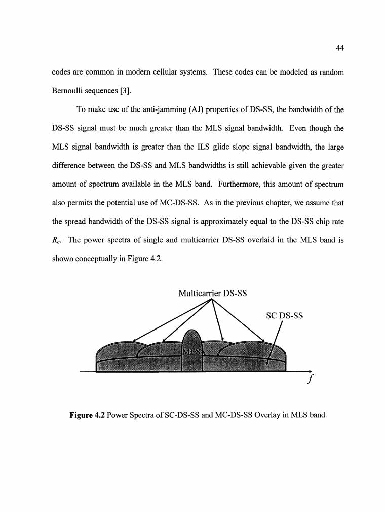
To make use of the anti-jamming (AJ) properties of DS-SS, the bandwidth of the
DS-SS signal must be much greater than the MLS signal bandwidth. Even though the
MLS signal bandwidth is greater than the ILS glide slope signal bandwidth, the large
difference between the DS-SS and MLS bandwidths is still achievable given the greater
amount of spectrum available in the MLS band. Furthermore, this amount of spectrum
also permits the potential use of MC-DS-SS. As in the previous chapter, we assume that
the spread bandwidth of the DS-SS signal is approximately equal to the DS-SS chip rate
R,. The power spectra of single and multicarrier DS-SS overlaid in the MLS band is
shown conceptually in Figure 4.2.
Multicarrier DS-SS
Figure 4.2 Power Spectra of SC-DS-SS and MC-DS-SS Overlay in MLS band.
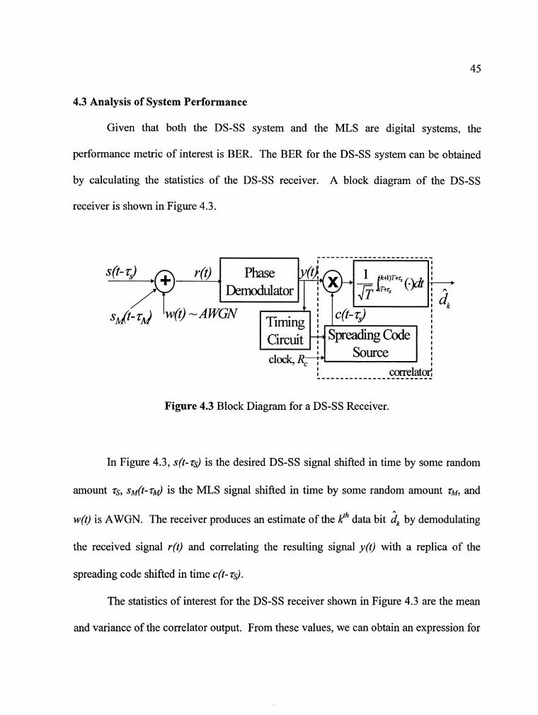
4.3 Analysis of System Performance
Given that both the DS-SS system and the MLS are digital systems, the
performance metric of interest is BER. The BER for the DS-SS system can be obtained
by calculating the statistics of the DS-SS receiver. A block diagram of the DS-SS
receiver is shown in Figure 4.3.
------------------------- I I
Phase I
I I I I I
I Spreading M e i Circuit 7 I
I Source clock, R c 7
I I I
I correlatorl -------------------------
Figure 4.3 Block Diagram for a DS-SS Receiver
In Figure 4.3, s(t-zs) is the desired DS-SS signal shifted in time by some random
amount zs, sM(t-zu) is the MLS signal shifted in time by some random amount z ~ , and
w(t) is AWGN. The receiver produces an estimate of the ph data bit ik by demodulating
the received signal r(t) and correlating the resulting signal y(t) with a replica of the
spreading code shifted in time c(t- zs).
The statistics of interest for the DS-SS receiver shown in Figure 4.3 are the mean
and variance of the correlator output. From these values, we can obtain an expression for
the SNIR. If we assume the processing gain of the DS-SS is large, the MLS interference
can be modeled as an additive Gaussian disturbance. The SNIR can be then be used to
determine the BER in a closed form solution via standard functions. The aforementioned
relationships are illustrated in (4-6).
In (4-6), Pb is the probability of bit error, S is the mean-square value of the desired DS-SS
signal, N is the variance of the AWGN, and I is the variance of MLS signal, all
conditioned upon a data bit +1 sent.
As noted in Chapter 3, in AWGN with no interference, the performance of
DS-SS with BPSK modulation is equal to that of un-spread coherent BPSK in AWGN,
which is given by Q ( J ~ ) , where Eb is the received bit energy and No is the one-
sided noise power spectral density. To account for the presence of the MLS signal, we
modify this in accordance with (4-6). Hence, we proceed as with the ILS interference
analysis of Chapter 3, and "feed" the MLS signal through the DS-SS receiver in Figure
4.3 and calculate the variance of the resulting output from the correlator ik.
Given the digital nature of both the MLS and DS-SS system, it becomes important
to take note of each systems respective data rate and their relationship. The MLS
transmits a data signal with a bit rate Rbp15.625 kbps. In general, the MLS data rate
will not be equal to the DS-SS data rate. Furthermore, it can be shown that the
DS-SS BER will be the same regardless of which system's data rate is greater, e.g.
RbfiRb, or Rb,&Rb, where Rb is the DS-SS bit rate. This assumption holds as long as the
DS-SS chip rate Rc is much greater than the MLS data rate RbM. With this in mind, we
have assumed that the DS-SS data rate is greater than the MLS data rate for the following
analysis, e.g. RbfiRb.
In addition to system data rates, we need to consider other MLS signal parameters
with respect to the DS-SS receiver. These parameters include the MLS signal amplitude,
the MLS signal delay, and the phase difference between the MLS and DS-SS signals.
For the following analysis, we examined a general expression. However, for some cases,
we assumed that both the DS-SS delay and the DS-SS phase were zero. In addition,
without loss of generality we considered the first DS-SS data bit do.
We have mentioned previously that the worst-case scenario for the DS-SS BER is
when the DS-SS and MLS carrier frequencies are equal. In some cases, we have assumed
that the MLS and DS-SS phases are equal and that the MLS data signal is time-aligned
with one of the DS-SS signal bit transitions. Use of these various assumptions in
different combinations allows study of average and worst-case conditions.
Using (4-I), (4-2), and Figure 4.3, we obtained a general expression for the MLS
component of the correlator output 2.. This expression is shown in (4-7).

In (4-7), m is the MLS component of the correlator output, A, is the constant amplitude
term, r is the MLS signal delay previously represented as r ~ , and the difference between
the DS-SS and MLS carrier frequencies is given as Af=fc-&. Given our previous
assumption of the DS-SS bit rate being greater than the MLS bit rate, m contains the
effect of at most two MLS data bits. These two MLS data bits correspond to the integrals
Il and 12. Note that the mean of (4-7) is zero due to the zero mean MLS data signal and
the zero mean DS-SS code chips.
For the next step, we simplify the integrals Il and 12. We begin by assuming the
delay r is random, and define it as follows:
In (4-8), k is a uniform integer random variable from 0 to N-1, and E is a continuous
uniform random variable distributed between 0 and 1. Substituting (4-8) into (4-7)
allows us to re-express the integrals Il and I2 in terms of DS-SS code chips. The integral
I1 can then be expressed in the manner shown in (4-9).
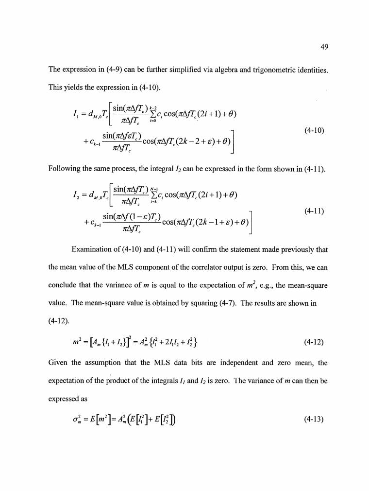
The expression in (4-9) can be further simplified via algebra and trigonometric identities.
This yields the expression in (4-1 0).
-
Following the same process, the integral I2 can be expressed in the form shown in (4-1 1).
Examination of (4-10) and (4-1 1) will confirm the statement made previously that
the mean value of the MLS component of the correlator output is zero. From this, we can
conclude that the variance of m is equal to the expectation of m2, e.g., the mean-square
value. The mean-square value is obtained by squaring (4-7). The results are shown in
(4- 12).
m = [A, ( I , + I, 1s = A: {I: + 2 I, I, + I: } (4- 12)
Given the assumption that the MLS data bits are independent and zero mean, the
expectation of the product of the integrals I] and I2 is zero. The variance of m can then be
expressed as
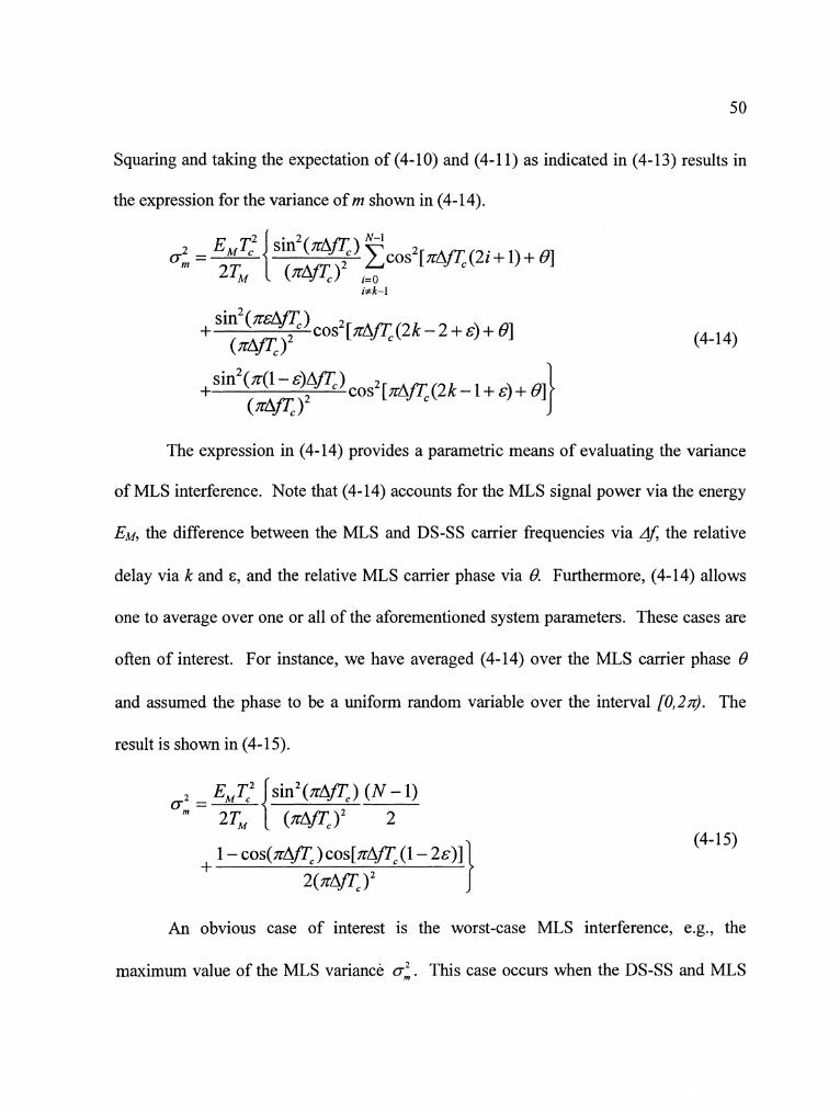
Squaring and taking the expectation of (4-10) and (4-1 1) as indicated in (4-13) results in
the expression for the variance of m shown in (4-1 4).
The expression in (4- 14) provides a parametric means of evaluating the variance
of MLS interference. Note that (4-14) accounts for the MLS signal power via the energy
EM, the difference between the MLS and DS-SS carrier frequencies via Af, the relative
delay via k and E, and the relative MLS carrier phase via 8. Furthermore, (4-14) allows
one to average over one or all of the aforementioned system parameters. These cases are
often of interest. For instance, we have averaged (4-14) over the MLS carrier phase 13
and assumed the phase to be a uniform random variable over the interval [0,24. The
result is shown in (4-15).
An obvious case of interest is the worst-case MLS interference, e.g., the
maximum value of the MLS variance a:. This case occurs when the DS-SS and MLS

carrier frequencies are aligned, the MLS phase 8 is zero, and the relative delay z is zero.
Substitution of these parameter values into (4-14) results in the relatively simple MLS
variance expression in (4- 16).
Another case of interest involves situating the DS-SS signal so that MLS carrier
frequency lies in the DS-SS signal's first spectral null. This means that the difference in
the DS-SS and MLS carrier frequencies is equal to the DS-SS chip rate, e.g., Af==tR,.
Such an arrangement results in substantially less interference between the two systems.
The resulting MLS variance expression is
Finally, we have averaged (4-14) over the delay z and the MLS phase 0 while
assuming an arbitrary difference in the MLS and DS-SS carrier frequencies. This results
in the complicated expressions shown in (4-18) and (4-19).
where
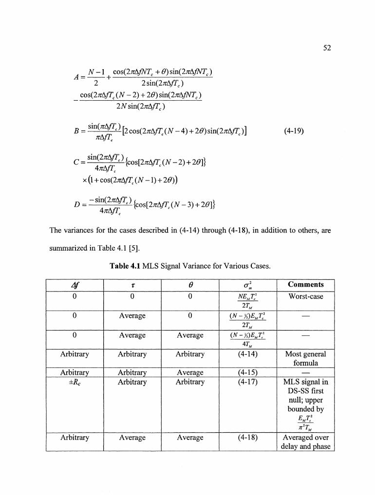
The variances for the cases described in (4-14) through (4-la), in addition to others, are
summarized in Table 4.1 [ 5 ] .
Table 4.1 MLS Signal Variance for Various Cases.
4f 0
0
0
Arbitrary
Arbitrary ~ R c
Arbitrary
z 0
Average
Average
Arbitrary
Arbitrary Arbitrary
Average
e 0
0
Average
Arbitrary
Average Arbitrary
Average
0;
NEM T: 2TM
( N - X)EME2 2TM
( N - K)E,T~'
4TM (4- 14)
(4- 15) (4- 17)
(4- 18)
Comments
Worst-case
-
-
Most general formula -
MLS signal in DS-SS first null; upper bounded by
E M T n2TM
Averaged over delay and phase

In Table 4.1, the term "Average" means that (4-14) was averaged over that
parameter. The distribution of the parameter is assumed to be uniform. In the case of the
delay z, the uniform distribution is between 0 and the DS-SS bit period T, e.g. the interval
z-U(0, T). Given the definition of the delay z given in (4-8), the integer DS-SS chip delay
k is a uniformly distributed integer from 0 to N-1, and the partial DS-SS chip delay E is
continuously distributed from 0 to 1. In the case of the MLS phase 6, the uniform
distribution is between 0 and 27c, e.g., the interval 8-U[O,2$. The term "Arbitrary"
means that the parameter can be given an arbitrary value.
Using one of the aforementioned MLS variance expressions, we can then
calculate the SC-DS-SS BER via substitution of said variance expression into (4-6), and a
small amount of algebra. This substitution results in the expression shown in (4-20).
Using (4-20) and a variance expression from Table 4.1, we can compute the error
probability of SC-DS-SS in the presence of AWGN and MLS interference. In (4-20), Eb
is the received DS-SS bit energy, No is the one sided power spectral density of AWGN,
oi is the variance of the MLS signal, and T is the DS-SS bit period.
4.4 Multicarrier DS-SS
MC-DS-SS techniques can also be used in the MLS band. The two cases of
interest are S:P conversion and splitting. These were discussed in Chapter 3. Once
again, little alteration of the previous results is required, and the multicarrier case is of
interest because not all the subcarriers need be affected by the MLS interference. Again,
the total bandwidth and the data rate of the multicarrier system should be equal to that of
the single carrier system to ensure an accurate comparison.
For multicarrier analysis, the SC-DS-SS signal defined in (4-3) is now considered
as one of M subcarrier signals. Then, with appropriate values for the DS-SS chip rate, the
DS-SS signal power, and the MLS signal power, the BER expression given in (4-20) can
be used to evaluate the error performance of a single DS-SS subcarrier. In most cases,
the DS-SS chip rate will still be much greater than the MLS data rate, e.g. Rc>>RbM [ 5 ] .
In the case of S:P conversion, the BER is found by calculating the average BER
over the M subcarriers. Assuming only one subcarrier incurs MLS interference, the
resulting BER expression is
In (4-21), PbA is the performance of the modulation in AWGN, and Pbl is the performance
in the presence of the MLS interference. For BPSK in AWGN with no interference, the
BER is given by (3-8). For BPSK in AWGN with MLS interference, the BER is given
by (4-20). It is important to point out that the MLS variance expression in (4-20) must
use the appropriate system parameter value, e.g. those of the MLS signal and the affected
MC-DS-SS subcarrier. The assumptions used to generate (4-16) represents the worst-
case scenario in terms of DS-SS BER. Substituting (4-16) into (4-20), we obtain the
expression for Pblwc shown in (4-22).
In (4-22), NMcI is the processing gain of the multicarrier system, PM is the received MLS
power, P is the received DS-SS power, Eb is the received DS-SS bit energy, M is the
number of subcarriers, and Pblwc is the probability of bit error for the multicarrier system.
The processing gain of the multicarrier and single carrier systems was shown to be equal
via (3-17).
The second MC case of splitting is the same as described in Chapter 3. The BER
for splitting is found in the manner shown in Chapter 3 with the exception that the MLS
variance is used. The resulting BER expression for splitting is shown in (4-24).
In this case, the multicarrier processing gain NMc2 is equal to the processing gain
of the single carrier divided by the number of subcarriers. This relationship was
illustrated in (3-20). Using worst-case DS-SS assumptions, e.g. Af= z=8=0, in (4-24), we
obtain the BER expression shown in (4-25).
In this case, the multicarrier BER is equal to that of the equivalent single carrier system
[5]. In (4-25), Nm2 is the processing gain of the multicarrier system, PM is the received
MLS power, P is the received DS-SS power, Eb is the received DS-SS bit energy, M is

the number of subcarriers, and Pb is the probability of bit error for the multicarrier
system.
4.5 Numerical Results
We now provide some examples using our analytical results, and corroborate
them with computer simulations. Using worst-case SC-DS-SS assumptions in the SC-
DS-SS BER expression in (4-20), we have plotted the analytical performance, e.g. Pb, of
a SC-DS-SS system in the presence of MLS interference for a range of processing gains
and JSR values. In this chapter, JSR is defined as the ratio of received MLS power to
received DS-SS power, PMS/PDs. The plots are shown in Figure 4.4.
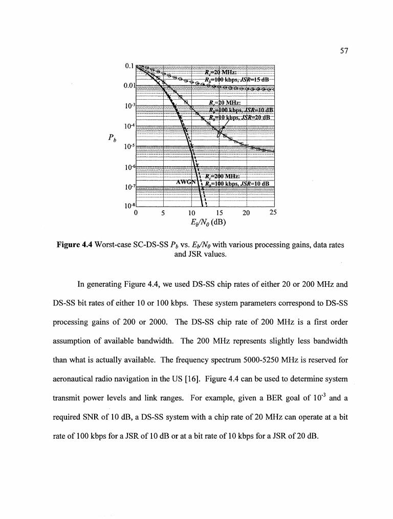
Figure 4.4 Worst-case SC-DS-SS Pb VS. EdNo with various processing gains, data rates and JSR values.
In generating Figure 4.4, we used DS-SS chip rates of either 20 or 200 MHz and
DS-SS bit rates of either 10 or 100 kbps. These system parameters correspond to DS-SS
processing gains of 200 or 2000. The DS-SS chip rate of 200 MHz is a first order
assumption of available bandwidth. The 200 MHz represents slightly less bandwidth
than what is actually available. The frequency spectrum 5000-5250 MHz is reserved for
aeronautical radio navigation in the US [16]. Figure 4.4 can be used to determine system
transmit power levels and link ranges. For example, given a BER goal of 10" and a
required SNR of 10 dB, a DS-SS system with a chip rate of 20 MHz can operate at a bit
rate of 100 kbps for a JSR of 10 dB or at a bit rate of 10 kbps for a JSR of 20 dB.
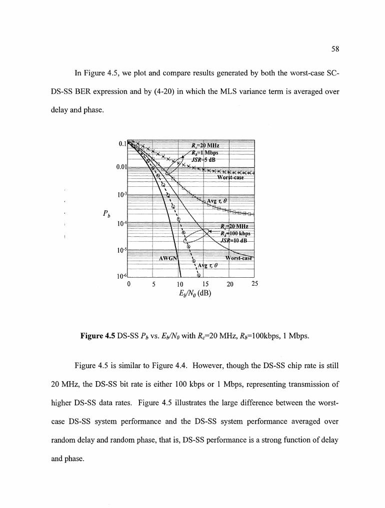
In Figure 4.5, we plot and compare results generated by both the worst-case SC-
DS-SS BER expression and by (4-20) in which the MLS variance term is averaged over
delay and phase.
Figure 4.5 DS-SS Pb VS. EdNO with R,=20 MHz, Rb=lOOkbps, 1 Mbps.
Figure 4.5 is similar to Figure 4.4. However, though the DS-SS chip rate is still
20 MHz, the DS-SS bit rate is either 100 kbps or 1 Mbps, representing transmission of
higher DS-SS data rates. Figure 4.5 illustrates the large difference between the worst-
case DS-SS system performance and the DS-SS system performance averaged over
random delay and random phase, that is, DS-SS performance is a strong function of delay
and phase.
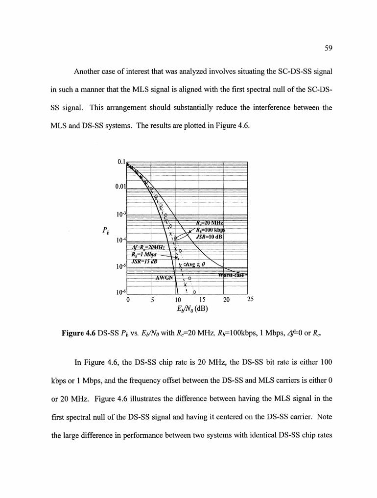
Another case of interest that was analyzed involves situating the SC-DS-SS signal
in such a manner that the MLS signal is aligned with the first spectral null of the SC-DS-
SS signal. This arrangement should substantially reduce the interference between the
MLS and DS-SS systems. The results are plotted in Figure 4.6.
Figure 4.6 DS-SS Pb VS. EdNO with Rc=20 MHz, Rb=lOOkbps, 1 Mbps, A P O or Re.
In Figure 4.6, the DS-SS chip rate is 20 MHz, the DS-SS bit rate is either 100
kbps or 1 Mbps, and the frequency offset between the DS-SS and MLS carriers is either 0
or 20 MHz. Figure 4.6 illustrates the difference between having the MLS signal in the
first spectral null of the DS-SS signal and having it centered on the DS-SS carrier. Note
the large difference in performance between two systems with identical DS-SS chip rates
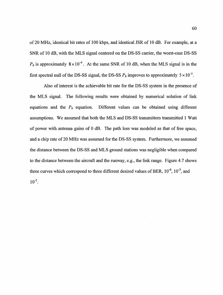
of 20 MHz, identical bit rates of 100 kbps, and identical JSR of 10 dB. For example, at a
SNR of 10 dB, with the MLS signal centered on the DS-SS carrier, the worst-case DS-SS
Pb is approximately 8 x 1 04. At the same SNR of 10 dB, when the MLS signal is in the
first spectral null of the DS-SS signal, the DS-SS Pb improves to approximately 5 x
Also of interest is the achievable bit rate for the DS-SS system in the presence of
the MLS signal. The following results were obtained by numerical solution of link
equations and the Pb equation. Different values can be obtained using different
assumptions. We assumed that both the MLS and DS-SS transmitters transmitted 1 Watt
of power with antenna gains of 0 dB. The path loss was modeled as that of free space,
and a chip rate of 20 MHz was assumed for the DS-SS system. Furthermore, we assumed
the distance between the DS-SS and MLS ground stations was negligible when compared
to the distance between the aircraft and the runway, e.g., the link range. Figure 4.7 shows
three curves which correspond to three different desired values of BER, 1 oe6, 1 o - ~ , and
1 o - ~ .

~d\i-ble Rb fw Pb=lO-6 ,Pb=103, end Pb=i0-2
10' 1 L .... : 1 I...- 1 , 1 1. i ...... ..I 10 20 30 40 50 60 70 80 90 100
Distance of DSSS Rx from DSSS Tx (km)
Figure 4.7 Achievable DS-SS data rate Rb (bps) for given Pb VS. link range, in presence of MLS.
As one would expect, the achievable DS-SS bit rate for a desired DS-SS BER
decreases as the distance between the DS-SS transmitter and DS-SS receiver increases.
This is due to signal attenuation from the free space path loss (i.e., normal SNR
reduction). In addition, the achievable DS-SS bit rate for a more stringent BER
requirement is smaller than the DS-SS bit rate for a less stringent BER requirement at a
given distance between the DS-SS transmitter and receiver. Finally, it is important to
point out that these results are for un-coded modulation, and hence not representative of
an actual system. The use of FEC would result in lower BER values or significantly
greater ranges.
In Figure 4.8, the BER for both analytical and simulated DS-SS in the presence of
MLS and AWGN is plotted as a function of SNR. In the simulation, the MLS and DS-SS
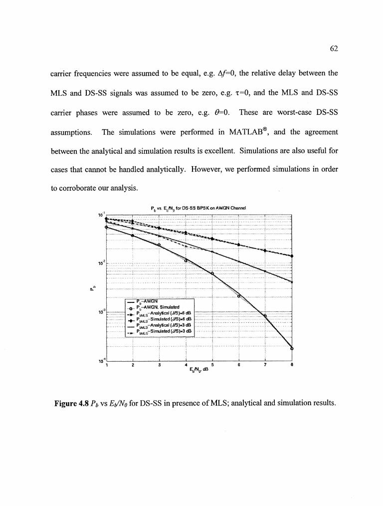
carrier frequencies were assumed to be equal, e.g. Af=O, the relative delay between the
MLS and DS-SS signals was assumed to be zero, e.g. z=0, and the MLS and DS-SS
carrier phases were assumed to be zero, e.g. 8=0. These are worst-case DS-SS
assumptions. The simulations were performed in MATLAB", and the agreement
between the analytical and simulation results is excellent. Simulations are also useful for
cases that cannot be handled analytically. However, we performed simulations in order
to corroborate our analysis.
Pb vs EtMO for DS-SS BPSKan AWGN Channel
d
+. Pa,,,- Simdnted (JIS).6 dB ,. PbM,,-Analybcal (JIS)-3 dB
1 2 3 4 5 6 7 E,M,, dB
Figure 4.8 Pb vs EJNO for DS-SS in presence of MLS; analytical and simulation results.

4.6 MLS Performance Degradation
As in the case of DS-SS spectral overlay in the ILS glide slope band, it is
important to quantify the degradation of the MLS signal due to the presence of the DS-SS
signal. This quantification is rather straightforward though as the DS-SS signal can once
again be approximated as AWGN. This DS-SS "noise" approximation is then added to
the original AWGN term. The DS-SS noise density approximation can be expressed as
IDS = PTM I(%) (4-26)
where P is the DS-SS power received by the MLS receiver, TM is the MLS bit period,
and R, is the DS-SS chip rate. The approximation given in (4-26) is good, even for DS-
SS bandwidths that are only a few times as great as the MLS bandwidth. Using (4-26)
results in the following MLS BER expression:
It is important to remember that (4-27) applies to differentially encoded bits, not
the actual MLS data bits. In the case that the BER expression in (4-27) falls below 0.01,
the BER of the actual MLS data bits may be accurately approximated by doubling the
value of (4-27) [5] .
It is possible to plot MLS performance in the presence of DS-SS interference for a
variety of parameters using (4-27). Some of these plots are shown in Figure 4.9.
Figure 4.9 MLS Ph VS. EdNo, for various JSR values.
In Figure 4.9, the DS-SS and MLS carrier frequencies are equal. The DS-SS chip
rate is either 20 or 200 MHz. In addition, as opposed to the previous plots, the JSR is the
ratio of DS-SS power to MLS power. The MLS BER increases as the JSR increases. For
example, assume a SNR of 10 dB and a DS-SS chip rate of 20 MHz. For a JSR of 10 dB,
the Ph is 2 x For a JSR of 15 dB, the Pb is and for a JSR of 20 dB, the Ph is
3 x This is expected, but note the difference in performance when the DS-SS chip
rate is increased from 20 MHz to 200 MHz. In this case, for a JSR of 28 dB and a SNR
of 10 dB, the resulting Pb is 9 x lo4.

We have shown the effect of the DS-SS ADL on the MLS signal in terms of
BER. Like the ILS, the MLS is a landing system, and it is important to translate the MLS
BER into the equivalent position error. This translation would give a better idea of the
effect the DS-SS ADL would have on MLS operation. Such a translation is left for future
work.
4.7 Summary
In the preceding sections, we examined the use of DS-SS spectral overlay in the
MLS band. Analytical techniques were used to obtain a BER expression for DS-SS with
BPSK modulation in the presence of AWGN and MLS interference. The results of this
analysis were then corroborated with MATLAB@ simulations. Example analytical and
simulated results were plotted for different parameter values. In addition, the effect of
DS-SS interference on the MLS was calculated and plotted for various parameters.
Chapter 5
System Comparisons
5.1 Introduction
In Chapters 3 and 4, we examined DS-SS spectral overlay in the ILS and MLS
spectral bands. In this chapter, we compare overlay results obtainable with the use of
these two bands. For such comparisons, we must select DS-SS system parameters.
These parameters are DS-SS bit rate, the number of DS-SS users, and the effective range
of the DS-SS link.
It is important of course that our comparison be fair. By fair, we mean that the
comparison accounts for the differences between the spectral bands. The two main
differences are the center frequencies and the bandwidths. The center frequencies are
also referred to as carrier frequencies, or often simply RFs. For instance, the ILS band
consists of the spectrum from 329 MHz to 335 MHz. This results in an approximate
bandwidth of 5 MHz. In the case of the MLS band, the frequencies range from 5091
MHz to 5 150 MHz for a bandwidth of approximately 60 MHz.
5.2 Center Frequency Considerations
The center frequencies are important to consider for two reasons. The first reason
is that path loss is frequency dependent. Before we illustrate this relationship, recall that
the frequency of an electromagnetic wave is equal to the speed of light divided by the

wavelength of the electromagnetic wave. This relationship was given in (2-2), and it
illustrates the inverse relationship between frequency and wavelength. Thus, a signal
transmitted in the ILS band will have a longer wavelength than that of a signal
transmitted in the MLS band.
Given that signals transmitted at higher frequencies have correspondingly shorter
wavelengths, a high frequency signal experiences greater free space loss at a given
distance than that of a signal transmitted at a lower frequency. This is shown in the
equation for path loss or free space loss, given in (2-1). Thus, the free space loss
experienced by a system operating in the MLS band will be greater than the loss
experienced by a system operating in the ILS band. For the same value of distance, the
MLS path loss will be approximately 25 dB greater than the ILS path loss. The greater
losses can be countered via higher transmit powers and higher gain antennas. The free
space path losses for ILS and MLS frequencies are plotted as a function of distance in
Figure 5.1.
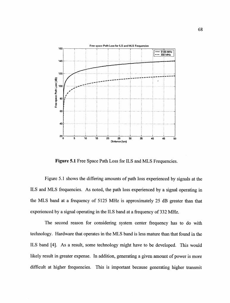
Free-srrace Path Loss for lLS and MLS Freauencies
Disttnce (km]
Figure 5.1 Free Space Path Loss for ILS and MLS Frequencies.
Figure 5.1 shows the differing amounts of path loss experienced by signals at the
ILS and MLS frequencies. As noted, the path loss experienced by a signal operating in
the MLS band at a frequency of 5125 MHz is approximately 25 dB greater than that
experienced by a signal operating in the ILS band at a frequency of 332 MHz.
The second reason for considering system center frequency has to do with
technology. Hardware that operates in the MLS band is less mature than that found in the
ILS band [4]. As a result, some technology might have to be developed. This would
likely result in greater expense. In addition, generating a given amount of power is more
difficult at higher frequencies. This is important because generating higher transmit
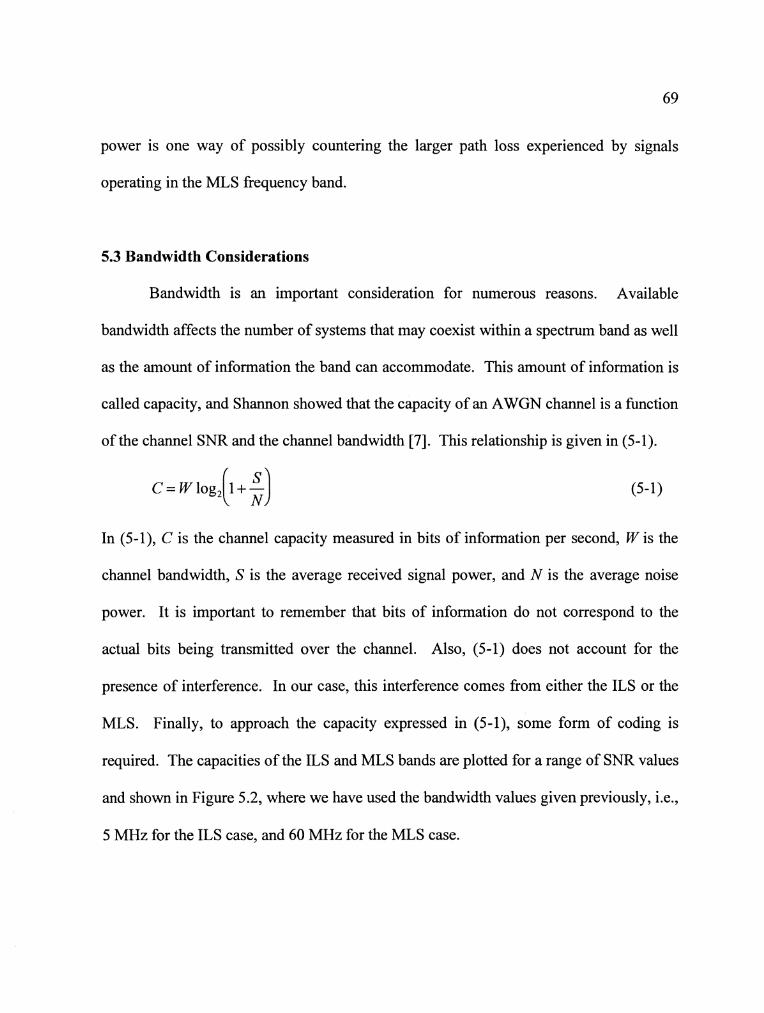
power is one way of possibly countering the larger path loss experienced by signals
operating in the MLS frequency band.
5.3 Bandwidth Considerations
Bandwidth is an important consideration for numerous reasons. Available
bandwidth affects the number of systems that may coexist within a spectrum band as well
as the amount of information the band can accommodate. This amount of information is
called capacity, and Shannon showed that the capacity of an AWGN channel is a hnction
of the channel SNR and the channel bandwidth [7 ] . This relationship is given in (5-1).
In (5-I), C is the channel capacity measured in bits of information per second, W is the
channel bandwidth, S is the average received signal power, and N is the average noise
power. It is important to remember that bits of information do not correspond to the
actual bits being transmitted over the channel. Also, (5-1) does not account for the
presence of interference. In our case, this interference comes from either the ILS or the
MLS. Finally, to approach the capacity expressed in (5-l), some form of coding is
required. The capacities of the ILS and MLS bands are plotted for a range of SNR values
and shown in Figure 5.2, where we have used the bandwidth values given previously, i.e.,
5 MHz for the ILS case, and 60 MHz for the MLS case.
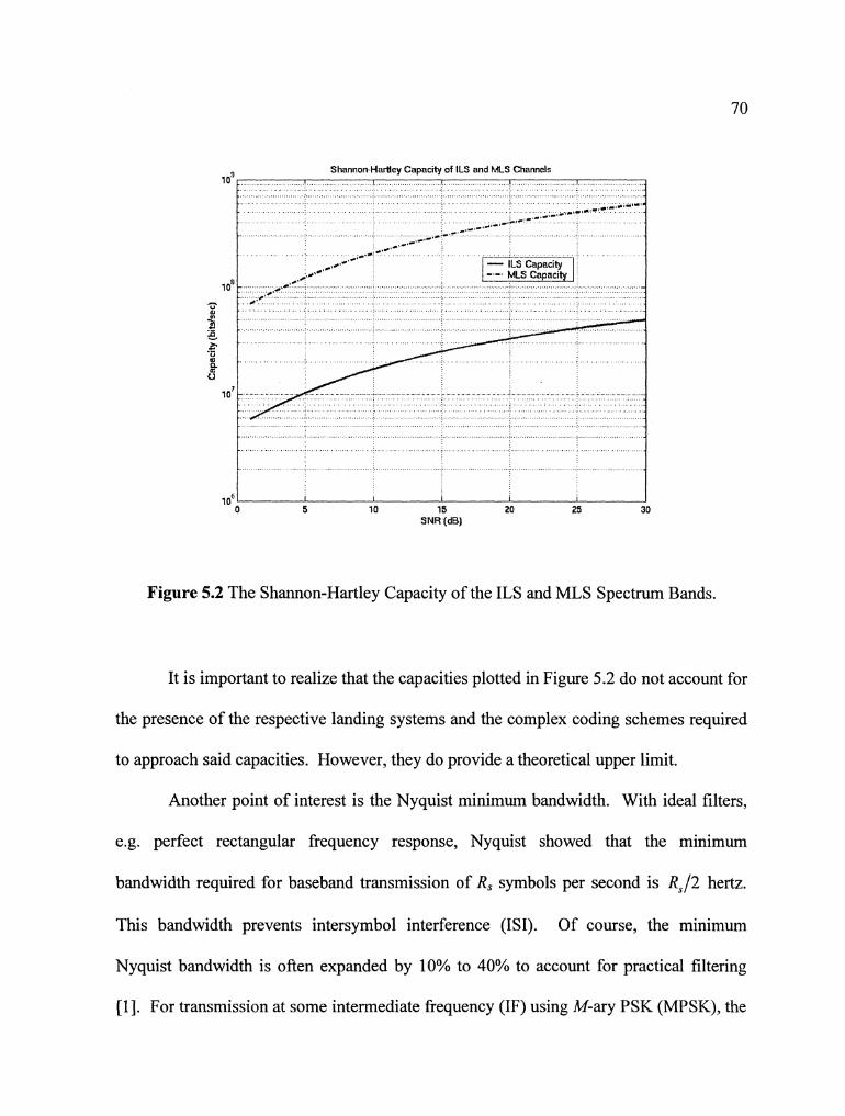
Shannon-Hartley Capaclty of ILS and MAS Channels lo9 , I
_ _ _,-.-z-l. - - _,_,--,- - - _ C - - _ -.a - - _.- -
+.-..c'~ - *. - ILS Capaclty
+so'e - -. MLS Capac~ty * \ * b e . * -
U
9
n 8
I
1 o6 I I I I I 0 5 10 15 20 25 30
SNR (dB)
Figure 5.2 The Shannon-Hartley Capacity of the ILS and MLS Spectrum Bands.
It is important to realize that the capacities plotted in Figure 5.2 do not account for
the presence of the respective landing systems and the complex coding schemes required
to approach said capacities. However, they do provide a theoretical upper limit.
Another point of interest is the Nyquist minimum bandwidth. With ideal filters,
e.g. perfect rectangular frequency response, Nyquist showed that the minimum
bandwidth required for baseband transmission of Rs symbols per second is R,/2 hertz.
This bandwidth prevents intersymbol interference (ISI). Of course, the minimum
Nyquist bandwidth is often expanded by 10% to 40% to account for practical filtering
[I]. For transmission at some intermediate frequency (IF) using M-ary PSK (MPSK), the

minimum double-sideband (DSB) bandwidth required for transmitting R, symbols per
second becomes R, hertz. Using our previous assumption of BPSK modulation, the
symbol rate translates to the bit rate. Furthermore, in the case of DS-SS, the symbol rate
translates to the chip rate.
Thus, given that both the ILS and MLS spectral bandwidths are limited via FAA
and FCC regulations, the Nyquist bandwidth predicts the highest chipping rate we can
hope to achieve. That rate is approximately 5 MHz in the ILS band and approximately
60 MHz in the MLS band.
With greater bandwidth, using more systems within a band may become feasible
via frequency division. In addition, available bandwidth is important when dealing with
DS-SS. More bandwidth allows for more spreading of the data signal, hence a greater
processing gain. In turn, a greater processing gain results in better interference protection
and the ability to support more users. In addition, with a larger processing gain, it is
possible to trade some of that gain for an increased bit rate. Finally, greater bandwidth
could also make the use of MC-DS-SS practical.
5.4 Band Limited and Power Limited Channels
We stated in the previous section that the bandwidths of the ILS and MLS spectra
are regulated via the FAA and FCC. In this way, both bands are bandwidth-limited.
However, when we speak of bandwidth-limited and power-limited channels in regards to
communication systems, we are usually discussing communication resources. By
resources, we mean those resources that are plentiful and those that are limited. Thus, the
bandwidth used by a bandwidth-limited channel is more valuable than bandwidth used by
a power-limited channel; the situation is reversed with respect to power. A channel can
be both power-limited and bandwidth-limited.
With a band-limited channel, a spectrally efficient modulation can be employed to
conserve bandwidth. However, the trade off involves transmitting more power. In the
case of a power-limited channel, a power efficient modulation can be used to conserve
power at the expense of expanded bandwidth. MPSK is a form of spectrally efficient
modulation while M-ary Frequency Shift Keying (MFSK) is considered power efficient
(111.
In the case of MPSK, the spectral efficiency can be better illustrated via (5-2).
In (5-2), R is the bit rate, W is the bandwidth, and M is the size of the signal alphabet. In
the case of BPSK, M is equal to two. The units of (5-2) are bits per second per Hertz
(bits/s/Hz). Note that as the size of the alphabet increases, so does the ratio of bit rate to
bandwidth, e.g. bandwidth efficiency increases. For BPSK, the bandwidth efficiency is
one bits/s/Hz. For 8-ary PSK, the bandwidth efficiency becomes three bits/s/Hz and so
forth. This increase in efficiency is due to the non-orthogonal nature of MPSK. A dense
MPSK alphabet requires no more bandwidth for transmission than a sparse MPSK
alphabet but requires more power for a constant level of performance (BER).
In the case of MFSK, the spectral efficiency is described by (5-3).
R - log, M W M
Once again, in (5-3), R is the bit rate, W is the bandwidth, and M is the size of the
alphabet. The units of (5-3) are also bits/s/Hz. However, note the difference between
(5-2) and (5-3). As the size of the alphabet M increases, the denominator in (5-3)
increases at a linear rate as opposed to the logarithmic rate of the numerator. As a result,
the spectral efficiency decreases. For BFSK, the efficiency is 112 bits/s/Hz. For 8-ary
FSK, the efficiency is 113 bits/s/Hz and so forth. The decrease in efficiency is due to the
orthogonal nature of MFSK. As symbols are added to the alphabet, the bandwidth must
be expanded so that the symbols remain orthogonal.
Spectral efficiency is an important consideration given the characteristics of both
the ILS and MLS spectral bands. We have already stated that both bands are band-
limited. They are also power-limited in the sense that performance degradation of the
respective landing systems beyond a certain point is unacceptable. The power limitations
are somewhat countered by the nature of DS-SS. Remember that the DS-SS energy is
spread over a large bandwidth. The spreading results in a reduced energy density for the
DS-SS signal, and the respective landing system receivers see the DS-SS signal as
additional AWGN. The reduced energy density allows for a tradeoff. A DS-SS system
could transmit more power and gain BER performance, or it could transmit more power,
gain spectral efficiency by using higher order MPSK, and sacrifice BER performance.
Ideally, a DS-SS system using MPSK modulation could decrease BER by transmitting

more power. Such a system would affect both the ILS and the MLS less than a
narrowband system transmitting the same amount of power.
5.5 Achievable Bit Rate, Number of Users, and Link Range
When considering an ADL that employs DS-SS CDMA, some of the parameters
of interest that come to mind immediately are the bit rates that can be achieved, and the
number of users the system can support. In Chapters 3 and 4, we plotted achievable bit
rates versus link distance for the ILS and MLS bands. We can combine these plots in
order to compare performance between the bands. The results are shown in Figure 5.3.
Figure 5.3 Achievable DS-SS Bit Rate Rb for a Single User in the ILS and MLS Bands for Transmit Power levels of 10 and 30 Watts.
In Figure 5.3, a target BER value of 10" was chosen, as were predetermined
transmit power levels of 10 and 30 Watts. In addition, antenna gains were set to unity (0
dB) for all cases. This is likely pessimistic for the MLS case, where smaller, more
directional antennas, are more feasible than in the ILS case. For a given transmit power,
the ILS, the MLS, and the DS-SS system transmits the same amount of power. In other
words, if the ILS is transmitting 10 Watts of power, then the MLS and DS-SS are also
transmitting 10 Watts each. This arrangement applies for the 30 Watt case as well. In
regard to power, the ILS system values are the pessimistic ones, since higher levels of
power are more easily generated in this band than at the MLS frequencies.
The DS-SS chipping rate in the ILS band is assumed to be 5 MHz, and the DS-SS
chipping rate in the MLS band is assumed to be 60 MHz. We use the same assumption
regarding distances as in previous chapters, namely that the distance between the
ILSIMLS and DS-SS transmitters is negligible when compared to the distance between
the transmitters and their respective receivers. In addition, since both the ILSIMLS and
DS-SS receivers are on the aircraft, the distance between them is assumed negligible as
well. In addition, both the DS-SS receiver operating in the ILS band and the DS-SS
receiver in the MLS band are assumed to have noise figures of 10 dB. Finally, we
assumed that there was only a single DS-SS user. The assumed parameter values are
summarized in Table 5.1.

Table 5.1 Numerical evaluation parameter values used to generate Figure 5.3.
In Table 5.1, PILs is the ILS transmit power, PMLs is the MLS transmit power,
PDsss is the DS-SS transmit power, Rclts is the DS-SS chipping rate in the ILS band, and
Rc MLS is the DS-SS chipping rate in the MLS band. In Figure 5.3, note the lower values
of achievable bit rates in the MLS band. For the higher transmit power, 30 Watts, the
highest achievable bit rate in the MLS band is approximately 2 kbps. For the lower
transmit power, 10 Watts, the highest bit rate is approximately 1.5 kbps. These bit rates
are approximately one order of magnitude less than those plotted for the ILS band, and
this is primarily due to the larger value of propagation path loss at the higher MLS
frequencies (see Figure 5.1).
The presence of multiple DS-SS users can have a detrimental affect on bit rate
due to the presence of additional interference in the form of multiple user interference
(MUI). Plots of DS-SS bit rate as a function of multiple DS-SS users are shown in Figure
5.4.

R , vs. Number of DSSS Uscrs for a Link Distance s 5 km loSr
f - ILS &DSSS P, * 10 W, PGILs=lOO
[ ,_. MLS &DSSS P,. 10 W, PQ,,*l200
i . 2 .
I
- 8 s -
3 kbps x 10 users s 300bpsX100users- 30 kbps tot+ ' . 30 kbps total
. 1 -
. , i , , , , , , ,
10' . <
150 bps X 'i I . - 360 users = I
i 45 kbps total
i I
i I I
10' : 3 , , $ 8 I
1 oU lo1 30 users lo' 1 0' Number of DSSS Users
Figure 5.4 Achievable DS-SS bit rate Rb (per user) versus the number of DS-SS users in the ILS and MLS bands, with a transmit power of 10 Watts, processing gains of 100 and
1200, and link distance of 5 krn.
In Figure 5.4, interference from the ILS and the MLS is taken into account. Note
the sharp decrease in bit rate that occurs for approximately 400 additional DS-SS users in
the MLS band and approximately 30 DS-SS users in the ILS band. The sharp decrease in
both cases is due to a "hard limit placed on the BER by the computer code used to
generate Figure 5.4.
In Figure 5.4, note that the number of DS-SS users that can be supported in the
MLS band is much greater than the number of DS-SS users that can be supported in the
ILS band. For example, the ILS band can support 10 DS-SS users operating at an

individual bit rate of 3 kbps. This results in a total bit rate of 30 kbps. The MLS band
can support 100 DS-SS users operating at an individual bit rate of 300 bps. This also
results in a total bit rate of 30 kbps. The MLS band can also support 300 DS-SS users
operating at an individual bit rate of 150 bps. This results in a total bit rate of 45 kbps.
The ratio of the number of DS-SS users K to DS-SS processing gain N, e.g. K/N, is
known as a load parameter, and system performance is expected to suffer as the load
parameter increases.
The number of additional DS-SS users is limited by the DS-SS processing gain.
For example, a DS-SS system with a processing gain of 25 cannot generally support more
than 25 users. The relationship between bit rate, chip rate, and processing gain was given
in (2-9), repeated here as N=RJRb, where N is the DS-SS processing gain, R, is the DS-
SS chip rate, and Rb is the DS-SS bit rate. Since the DS-SS chip rate is limited by the ILS
and MLS bandwidths, the DS-SS bit rate is limited for a given value of processing gain.
Plots of DS-SS bit rate as a function of distance and MU1 are shown in Figure 5.5.

Figure 5.5 Achievable DS-SS bit rate Rb (per user) in the ILS and MLS bands for transmit power level of 10 Watts in the presence of MUI.
Ach~evable Rb for Pb=103 for a DSSS User wl MU1
The plots in Figure 5.5 were made using the same assumptions used to
generate those in Figure 5.3. A BER value of 10" was used, and the transmit power of
the ILS, the MLS, and the DS-SS are assumed to be equal. However, only one value of
transmit power, 10 Watts, was used, in order to clearly show the effect of MUI. In Figure
5.5, K represents the number of additional DS-SS users. In addition, a greater value of
processing gain is used in the MLS band than in the ILS band, 1200 as opposed to 100.
This is done to account for the difference in available bandwidth in the ILS and MLS
bands. Since we have assumed the MLS bandwidth to be twelve times greater than the
ILS bandwidth, 60 MHz as opposed to 5 MHz, the MLS processing gain is twelve times
50
I
Distance of DSSS Rx from DSSS Tx (km)
- ILS & DSSS. Pt=10 W, K=20, PG=lOO --. MLS & DSSS: Pt=10 W. K=240, PG=1200 a- ILS & DSSS P,=lO W, K=30. PG=IOO
-
+- MLS & DSSS P,=lO W, K=360. PG=lmO ,
*n-*-+-%--a b - c - n - u - w - - r - - * -
10'
: ", t,,,-, %\
ai '--------. ~-O-Q-+Q-O-C~.-~-+:--
I I I 1 I I I
5 10 15 20 25 30 35 40 45

greater than the ILS processing gain. Finally, we assume that there are twelve times as
many DS-SS users in the MLS band as there are in the ILS band. This is done to keep
the respective load factors equal. One set of plots is for a DS-SS load factor of 115, and
the other set is for a load factor of approximately 113. The plotted bit rate is the bit rate
for a single DS-SS user, i.e., the per-user bit rate for all K users.
Note the clear difference in achievable bit rate between the two. In the ILS band,
with a DS-SS load factor of 115, the bit rate starts at approximately 10 kbps and drops to
approximately 1 kbps at a distance of twelve kilometers. In the ILS band, with a load
factor of 113, the bit rate drops from 5 kbps to 500 bps over the first twelve kilometers.
In the MLS band, with a load factor of 115, the bit rate drops from 650 bps to 85 bps over
the first twelve kilometers. With a load factor of 113 in the MLS band, the bit rate drops
from 250 bps to the minimum bit rate supported by the numerical evaluation, 25 bps, in
the first five kilometers.
The plots in Figures 5.3 and 5.5 are similar, but the effect of MU1 is visible. For
example, at a distance of 10 kilometers, without MUI, the DS-SS bit rate in the ILS band
is approximately 2 kbps. With MUI, a load factor of 115, the DS-SS bit rate is
approximately 1.25 kbps. With a load factor of 113, the bit rate is 500 bps. At a distance
of 40 kilometers, in the ILS band without MUI, the bit rate is 500 bps. With a load factor
of 115, the bit rate is 300 bps. With a load factor of 113, the bit rate is 150 bps. DS-SS
bit rates in the MLS band exhibit similar trends. In the MLS band without MUI, the DS-
SS bit rate falls from 1.5 kbps to 150 bps in the first fifteen kilometers. With a load

factor of 115, the bit rate falls from 650 bps to 55 bps in the first fifteen kilometers while
with a load factor of 1/3, the bit rate falls fkom 250 bps to the numerical evaluation
minimum of 25 bps.
The presence of MU1 was modeled using the standard Gaussian assumption
(SGA). This assumption is shown below in (5-4).
BE" = {{F] effective = ('1 No + 0,s +I0
In (5-4), BER is the bit to error ratio, (E,/N,)~@.~~ is the effective SNR, and as in
Chapters 3 and 4, Eb is the received DS-SS bit energy, No is the power spectral density of
one sided AWGN, 02, is the variance of the respective landing system signal, and the
new term I, is the MU1 term. The MU1 term is taken from [lo] and is defined in (5-5).
In (5-5), N is the DS-SS processing gain, K is the number of users, Eb is the
received DS-SS bit energy, and a is a parameter that accounts for assumptions regarding
chip timing and carrier phase of the multiple users. For example, a a value of unity
would mean that we are assuming that both the chip timing and carrier phase of all the
users are aligned. In the numerical evaluations used to generate Figures 5.4 and 5.5, we
used a a v alue o f t hree. T his v alue assumes random chip timing and random c arrier
phase. A range of a values and the corresponding assumptions are given in Table 5.2. In
addition, (5-5) assumes that all K-user signals are received by a DS-SS receiver with

equal energy. Hence, this would be a good model for the GA link, where all K signals
originate from a common ground site. The use of the SGA is actually pessimistic in this
GA case, since MU1 can be near zero if synchronous, orthogonal spreading codes are
used.
Table 5.2 MU1 a Parameter Values and Corresponding Assumptions.
-
In addition to the single user bit rate, we can also plot the total bit rate in both the
ILS and MLS bands. The total bit rate is equal to the single user bit rate multiplied by the
number of DS-SS users, or R, x K . The total bit rates in both the ILS and MLS bands
are plotted in Figure 5.6.
a 1 2
2.5 3
Assumptions DS-SS chip timing aligned, DS-SS carrier phase aligned DS-SS chip timing aligned, Random DS-SS carrier phase Random DS-SS chip timing, DS-SS carrier phase aligned Random DS-SS chip timing, Random DS-SS carrier phase

Total R , us Number of DSSS Users for a Link Distance - 5 km
Number of DSSS Users
Figure 5.6 Achievable DS-SS total bit rate versus the number of DS-SS users in the ILS and MLS bands, with a transmit power of 10 Watts, processing gains of 100 and 1200,
and link distance of 5 krn.
The plots in Figure 5.6 were generated using the same assumptions used in
generating Figure 5.4. Initially, the total DS-SS bit rate in the ILS band is greater than
the total bit rate in the MLS band by approximately one order of magnitude. This
remains the case until the number of DS-SS users approaches 30. At this point, the ILS
plot is cut-off due to the aforementioned "hard" limit on DS-SS BER. The MLS plot
surpasses the ILS plot for approximately 50 DS-SS users. Both the ILS and MLS bands
exhibit similar total bit rate performance. However, this performance occurs for different
ranges of DS-SS users. For example, the total bit rate in the ILS band is between 30 kbps

and 50 kbps for a range of DS-SS users from 10 to 30. In the MLS band, the total bit rate
is also between 30 kbps and 50 kbps for a range of 100 and 350 DS-SS users. This
means that the MLS band can support approximately one order of magnitude more DS-
SS users than the ILS band. However, this comes at the cost of a single user bit rate
which approximately one order of magnitude less than that in the ILS band.
Neither Figure 5.4 nor 5.6 account for antenna gain. The use of higher
transmit powers andlor higher antenna gains would result in greater single and total bit
rates. As an example, Figure 5.7 shows achievable bit rates for the same conditions as in
Figure 5.6, except that both the transmit and receive antenna gains in the MLS band are
equal to 10 dB. This results in a net antenna gain of 20 dB.
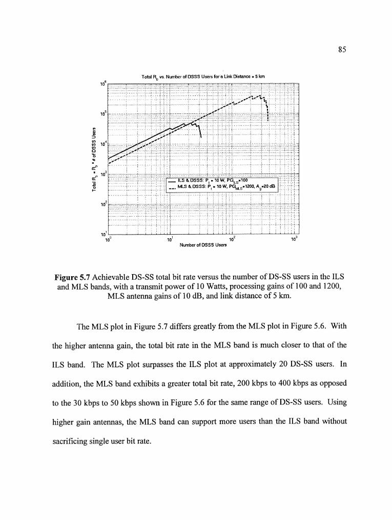
Total R, us Number of DSSS Users for a Link Distance = 5 km
i 10' ' I I
I I
1 oL 10' lo2 loJ Number of DSSS Usen
Figure 5.7 Achievable DS-SS total bit rate versus the number of DS-SS users in the ILS and MLS bands, with a transmit power of 10 Watts, processing gains of 100 and 1200,
MLS antenna gains of 10 dB, and link distance of 5 km.
The MLS plot in Figure 5.7 differs greatly from the MLS plot in Figure 5.6. With
the higher antenna gain, the total bit rate in the MLS band is much closer to that of the
ILS band. The MLS plot surpasses the ILS plot at approximately 20 DS-SS users. In
addition, the MLS band exhibits a greater total bit rate, 200 kbps to 400 kbps as opposed
to the 30 kbps to 50 kbps shown in Figure 5.6 for the same range of DS-SS users. Using
higher gain antennas, the MLS band can support more users than the ILS band without
sacrificing single user bit rate.
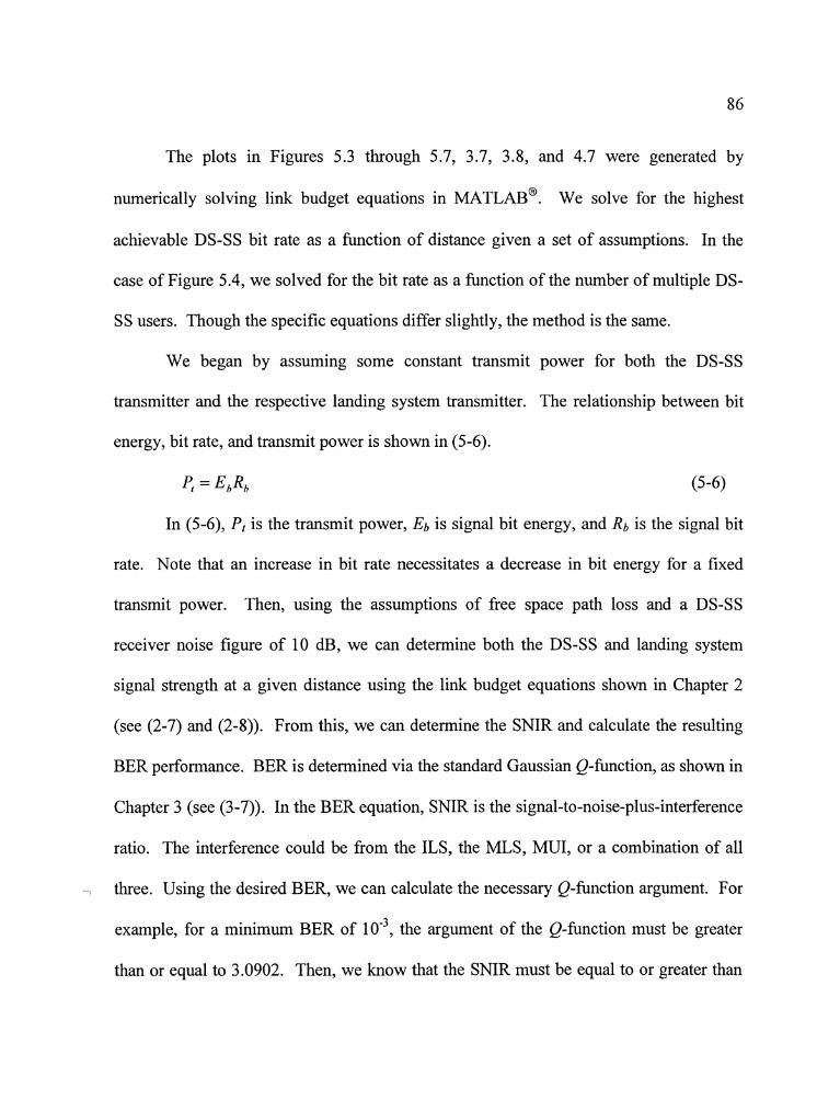
The plots in Figures 5.3 through 5.7, 3.7, 3.8, and 4.7 were generated by
numerically solving link budget equations in MATLAB@. We solve for the highest
achievable DS-SS bit rate as a function of distance given a set of assumptions. In the
case of Figure 5.4, we solved for the bit rate as a function of the number of multiple DS-
SS users. Though the specific equations differ slightly, the method is the same.
We began by assuming some constant transmit power for both the DS-SS
transmitter and the respective landing system transmitter. The relationship between bit
energy, bit rate, and transmit power is shown in (5-6).
P, = EbRb (5-6)
In (5-6), P, is the transmit power, Eb is signal bit energy, and Rb is the signal bit
rate. Note that an increase in bit rate necessitates a decrease in bit energy for a fixed
transmit power. Then, using the assumptions of free space path loss and a DS-SS
receiver noise figure of 10 dB, we can determine both the DS-SS and landing system
signal strength at a given distance using the link budget equations shown in Chapter 2
(see (2-7) and (2-8)). From this, we can determine the SNIR and calculate the resulting
BER performance. BER is determined via the standard Gaussian Q-function, as shown in
Chapter 3 (see (3-7)). In the BER equation, SNIR is the signal-to-noise-plus-interference
ratio. The interference could be from the ILS, the MLS, MUI, or a combination of all
- three. Using the desired BER, we can calculate the necessary Q-function argument. For
example, for a minimum BER of lo5, the argument of the Q-function must be greater
than or equal to 3.0902. Then, we know that the SNIR must be equal to or greater than
the square of 3.0902 to ensure the desired BER performance. With this in mind, we can
use MATLAB@ to determine the highest permissible bit rate for a given distance.
Figures 5.3 and 5.5 also illustrate the effective link range to a certain degree. In
the MLS band, the achievable bit rate falls to 300 bps or less in the first 10 kilometers.
These low values of achievable bit rate are due to the small value of transmit power, and
unity-gain antennas. If larger values of transmit power and/or directional antennas were
used, the bit rates would be significantly larger. As an illustration of this, Figure 5.8
shows achievable bit rates for the same conditions as in Figure 5.5, except that both the
transmit and receive antenna gains in the MLS band are equal to 10 dB. This results in a
net antenna gain of 20 dB.
Figure 5.8 Achievable DS-SS bit rate Rb (per user) in the ILS and MLS bands for transmit power level of 10 Watts in the presence of MU1 and antenna gains of 10 dB.
Achievable Rb for Pb=10'3 for a DSSS User w/ MU1
50
I I
Distance of DSSS Rx from DSSS Tx (km)
- ILS & DSSS P,=IO W K=20, PG=100 --. MLS & DSSS Pt=IO W, K=240, PG=lMO, Ag=20 dB -*. ILS 8 DSSS PI=IO W, K=30. PG=100
.
9- MLS & DSSS PI=10 W. K=360. PG=1200, Ag=20 dB ,
*-*-*-*--**c----------------.
' b - r e - 8 - u - u - r - - x -
b-9-+0:
10' ; I I I I t I 1
10 15 20 25 30 35 40 45

As expected, the achievable bit rates in the MLS spectral band are greater with the
use of directional antennas than without. In general, the bit rate is increased by one order
of magnitude. For example, at a distance of 10 kilometers, in the MLS band with a load
factor of 115, the bit rate increases from 75 bps to 750 bps. With a load factor of 113, in
the MLS band, the bit rate increases from 25 bps to 250 bps. This increase may be
pessimistic in that the minimum bit rate used by the numerical solution is 25 bps. This
minimum bit rate is important to keep in mind when examining the MLS plots in Figures
5.3, 5.5 and 5.8, especially when the link distance exceeds 10 kilometers.
Given the nature of airport traffic, it is more realistic to examine achievable bit
rate of both the ILS and MLS bands for a fixed number of DS-SS users, in other words to
disregard the respective load factors and assume each band has the same number of DS-
SS users. The results of such a numerical evaluation are shown in Figure 5.9.

Achievable R!, for P,,-10 3 for a DS SS User wt MU1
Distance of DSSS Rx from DSSS Tx (km)
10" t : ! ,
Figure 5.9 Achievable DS-SS bit rate Rb (per user) in the ILS and MLS bands for transmit power level of 10 Watts in the presence of equal MU1 and antenna gains of 10
and 15 dB.
I t
1oSr - -
Most of the assumptions used to generate Figure 5.8 were used to generate Figure
5.9. The differences are that both the ILS and MLS bands were assumed to have an equal
number of DS-SS users, 20 or 30, and an additional MLS result was plotted with antenna
gains of 15 dB. This results in a net antenna gain of 30 dB. This was done in order to
- ILS & DSSS P,.10 W, K-20, PG-100 ,,. MLS b DSSS P,.10 W. K-20, PG=1200. Ag=20 dB ,. ILS & DSSS P,-10 W, K.30, PG.100 +. MLS (C DSSS. P,-10 W, K-30, PG-1200, As= 20dB
MLS b DSSS P,-10 W. K.30, PG.1200 AS. 30dB
improve visual clarity, as three of the plots in Figure 5.9 are virtually indiscernible.
In Figure 5.9, the DS-SS bit rate in the ILS band is the same as that shown in
Figure 5.8. However, in Figure 5.9, the DS-SS bit rate in the MLS band has improved
such that it is equal to that of the ILS band for a load factor of 115 regardless of the MLS
E
-*-,,. $3
load factor. Note that the load factor of the DS-SS system in the MLS band has been
reduced to 1/60 for 20 DS-SS users and 1/40 for 30 DS-SS users. This negligible
difference in load factor explains the similarity of the DS-SS bit rates in the MLS band.
It is important to realize that these bit rates do not account for the use of coding.
The use of FEC would result in lower channel error probabilities. Assuming constant
transmit power, a reduction in error probability could be traded off for a larger bit rate.
In addition, for a fixed BER, the use of FEC would reduce the required SNIR.
5.6 Conclusions
Given our assumptions, it would seem that the ILS band is a better candidate for a
data link because of better signal propagation. The ILS carrier frequencies experience
better propagation conditions than the higher MLS frequencies. In turn, ILS propagation
allows for greater achievable bit rates than those of a MLS band data link that uses equal
transmit power. For this reason, the MLS band could be used for short-range
applications. However, our assumptions did not account for the use of directive or high
gain antennas. The use of such antennas would help counter the greater free space loss
experienced at MLS frequencies. For example, in a realistic case, the ILS transmit power
might be 10 dB greater than the MLS transmit power. MLS antennas with gains 10 dB
greater than those of the ILS antennas would result in a net 10 dB boost to the MLS link.
The use of directive antennas could also affect the ability of the ADL to support multiple
users.
The MLS band is still appealing due to the greater available bandwidth. The
MLS bandwidth is approximately 12 times greater than the ILS bandwidth. This results
in a larger information capacity, and this greater capacity allows more information to be
sent across the channel. In addition, the greater bandwidth could possibly be used for a
MC-DS-SS ADL. In terms of frequency and spectra, a MC-DS-SS ADL could be
situated around the narrowband landing system signals as to minimize interference. In
fact, the key difference i n p erformance b etween a S C-DS-SS signal and a M C-DS-SS
signal is due to the notion that not all of the MC-DS-SS subcarriers are necessarily
affected by the landing system signals. However, a multiple carrier scheme would also
be more complex than a single carrier alternative.
Chapter 6
Summary and Conclusions
6.1 Summary
In this thesis, we examined the use of spectral overlay of DS-SS CDMA in the
ILS glide slope and MLS spectral bands as a potential ADL. We began by exploring
ADL design issues. These included defining the channel model: free space propagation
model and AWGN. While this model is a first-order one, it represents a starting point for
future studies and gives insight into the potential of the technique. We discussed the ILS
glide slope and MLS spectral bands, their respective characteristics, and the effects these
characteristics would have on a DS-SS CDMA ADL.
The scenario we considered involved using DS-SS CDMA in spectral overlay
mode. Spectral overlay is a means of increasing spectral efficiency, in other words
allowing for higher data throughput. Spectral overlay achieves this by allowing the DS-
SS signal to "coexist" with the respective landing signal in the same band, at the same
time. We examined the performance degradation experienced by the DS-SS CDMA, the
ILS, and the MLS systems because of this coexistence. In addition, we explored the use
of both SC-DS-SS and MC-DS-SS.
Our analysis involved classical analytical techniques as well as computer
simulations and numerical evaluations. The simulations were performed in order to
corroborate our analytical findings. We used the numerical evaluations to estimate
system performance. Plots were generated for a range of DS-SS CDMA and landing
system parameters.
In addition, we compared potential DS-SS CDMA performance when used in
either the ILS glide slope or MLS spectral bands. Our main performance metrics were
ADL bit rate, the number of users supported by the ADL, and the effective link range of
the ADL. We also looked at the Shannon capacity of each spectral band, the effect of
center frequency on signal propagation, and the difference in available bandwidths
between the spectral bands.
6.2 Conclusions
In conclusion, the application of spectral overlay in both the ILS and MLS
spectral bands is feasible given some small degradation to ILS or MLS performance. In
the case of the ILS, this degradation would be either a reduced SNR or a slightly reduced
effective range. For the MLS, this degradation would be either a small increase in the
MLS BER or a slightly reduced effective range. In either case, a careful ADL system
design is necessary.
Both the ILS and MLS spectral bands show promise for an ADL. In the case of
the ILS band, better propagation conditions allow for a greater link range. The better
propagation conditions are due to the lower carrier frequency. In the MLS band, the
propagation conditions are much worse than those found in the ILS band, but this could
be somewhat countered by the use of directional antennas with a high gain. Such
antennas could possibly limit the effectiveness of the ADL in a multiple user scenario

through increased complexity at either the ground-based transceiver or the transceiver on
the aircraft.
However, the MLS band possesses approximately twelve times as much
bandwidth as the ILS band. The greater bandwidth allows for more spreading by the DS-
SS CDMA signal, a greater ADL data rate, and better protection from interference. In
addition, if supportable link distance is not the primary concern, the greater MLS
bandwidth could support a much larger number of simultaneous users than the ILS band,
roughly 12 times. In addition, the greater bandwidth can be used for MC-DS-SS.
However, the advantages of a multiple carrier system over a single carrier system are, in
this case, relatively small, and primarily appear to be in the flexibility they provide for
different data rates, and band partitioning.
6.3 Areas for Future Work
There are several areas for future work in regards to this topic. A logical
extension of our parametric approach would be to obtain explicit values for ILS and MLS
parameters. These would include the minimum acceptable ILS SNR, the minimum
acceptable MLS BER, typical and maximum transmit powers, ILS and MLS receiver
filter bandwidths, typical receiver noise figures, and realistic link ranges. With these
parameters, it would be possible to more accurately predict the effects of the DS-SS ADL
on the respective landing systems, as well as place limits on ADL parameters such as
transmit power and the number of supportable users.

Another area for future work would be the exploration of orthogonal spectral
allocations for the ADL with respect to the landing system signals. Spectral overlay is
something of a worst-case scenario in terms of intersystem interference. Orthogonal
spectral allocation could significantly reduce intersystem interference.
Another area for future work would be using different channel and propagation
models. The channel model could account for fading and multipath, both of which would
be important considerations if the ADL were employed in a GG scenario or at low
elevation angles. The GG scenario is of particular interest for possible communication
along the airport surface itself. In addition, the analysis in the previous chapters does not
account for the use of FEC. Powerful FEC codes would certainly be used, and they
would reduce BER. This lower BER could then be traded for a higher bit rate.
Another area of interest would be the use of directive antennas to counter the
relatively poor propagation conditions found in the MLS band. The effects of directive
antennas on the ADL ability to support multiple users would have to be considered as
well, and for this, initial inquiries would likely begin with terrestrial cellular systems,
where much research on directive antennas has been done.
Finally, an important area for future work would be to translate the effect of the
DS-SS ADL into position error for the respective landing systems. In the case of the ILS,
this would involve using the ILS SNIR to determine position error. In the case of the
MLS, this would involve using the MLS BER to determine position error. Furthermore,
given the digital nature of the MLS, it might be necessary to examine the effect the ADL
would have on MLS signal acquisition and tracking.
References
[I] Sklar, B., Digital Communications Fundamentals and Applications, Second
Edition, Prentice-Hall, Inc., Upper Saddle River, NJ, 2001.
[2] Matolak, D., W., Neville, J., T., "Spectral Overlay of Direct-Sequence Spread
Spectrum in the Instrument Landing System Glideslope Band for Airborne
Internet," Proc. 22"' Digital Avionics Systems Conference, Indianapolis, IN,
October 2003.
[3] Peterson, R., L., Ziemer, R., E., Borth, D., E., Introduction to Spread Spectrum
Communications, Prentice-Hall, Upper Saddle River, NJ, 1995.
[4] Matolak, D., W., "Alternative Communications Spectrum Study for Aviation Data
Links," Project Final Report, NASA grant NAG3-28 15, July 2003.
[5] Matolak, D., W., Neville, J., T., "Spectral Overlay of Direct-Sequence Spread
Spectrum in the Microwave Landing System Band," Proc. 2jth IEEE Aerospace
Conference, Big Sky, MT, March 2004.
[6] Kayton, M., Fried, W., Avionics Navigation Systems, Second Edition, John Wiley
& Sons, Inc., New York, NY, 1997.
[7] Shannon, C.E., "A Mathematical Theory of Communication," The Bell System
Technical Journal, vol. 27, 1948, pp. 379-423,623-657.
[8] Department of Transportation, Federal Aviation Administration (FAA) National
Airspace System (NAS) website,
http://www 1 . f a a . g o v / n a s a r c h i t e c t u r e / b l , 27 January 2004.

[9] Simon, M. K., Omura, J. K., Scholtz, R. A., and Levitt, B. K., Spread Spectrum
Communications, Vol. 2, Computer Science Press, Inc., Rockville, MD, 1985.
[lo] Stuber, G., L., Mobile Communications, Second Edition, Kluwer Academic
Publishers, Boston, MA, 2000.
[ l l ] Proakis, J., G., Digital Communications, Second Edition, McGraw-Hill, New
York, NY, 1989.
[12] Stallings, W ., D ata & C omputer C ommunications, S ixth Edition, P rentice-Hall,
Upper Saddle River, NJ, 2000.
[13] Bello, P., A., "Generic Channel Simulator," Chapters 8 & 9, Technical Report
from BELLO, Inc., Contract MDA904-95-C-2078, February 1997.
[14] Elnoubi, S., M., "Capacities of Mobile AirIGround Radio Communication
Systems Employing Cylindrical Cells," IEEE Transactions on Aerospace and
Electronic Systems, vol. 34, no. 1, January 1998.
[15] Matolak, D., W., "On the Capacity of CDMA and TDMA Systems for the VHF
Air-to-GroundIGround-to-Air Communications," MITRE Technical Report
97W0000038, December 1997.
[16] The National Telecommunications and Information Administration (NTIA)
website, www.ntia.doc.gov/osmhome/ch04chart.pdf7 12 February 2004.

Appendix
MATLAB' Code
o/o=================================
% Function 0ffCenterSingleToneJam.m % Original program, DSSSBPSKsim.m provided by Dr. David Matolak
o----------------------------------
% OffCenterSingleToneJam runs a DS-SS BPSK simulation % over an AWGN Channel with a tone jammer that does % not share the carrier frequency of the system. % Currently configured to use either short or long random spreading % codes, with the same, or a new code for each of Nav trials. clear all; yplot=l ; % Set yplot=l to plot Pb vs. Eb/NO ncode=O; % Set ncode=l to use new spreading code for each of Nav trials % (one trial goes through range of SNRs) Codetype=l; % Set Codetype=O for short codes, 1 for long codes if ncode == 0
if Codetype == 0 zc=O; % Same code for each of Nav trials, short code
else zc=l; % Same code for each of Nav trials, long code
end else
if Codetype == 0 zc=2; % New code for each of Nav trials, short code
else zc=3; % New code for each of Nav trials, long code
end end Eb= l ; % Normalize bit energy to unity Nav=2; % Set number of trials to run at any given SNR Smin=l ; % minimum value of Eb/NO, in dB Smax=5; % maximum value of Eb/NO, in dB Sinc=l ; % Eb/NO increment, in dB S=[Smin:Sinc:Smax]; Ls=length(S); gbn=l O.A(S/lO); % SNR vector, numeric J=9; % Set J/S power ratio, in dB J2=3;
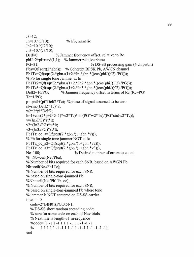
J3=12; Jn=1 O."(J/lO); % J/S, numeric Jn2=1 O."(J2/10); Jn3=1O."(J3/10); Delf=O; % Jammer frequency offset, relative to Rc phiJ=2*pi*rand(l, 1); % Jammer relative phase PG=3 1 ; % DS-SS processing gain (# chipslbit) Pba=Qf(sqrt(2*gbn)); % Coherent BPSK Pb, AWGN channel Pbl Tz=Qf(sqrt(2.* gbn./(1+2.* Jn. *gbn.*((cos(phiJ))"2).IPG))); % Pb for single tone Jammer at fc Pbl Tz2=Qf(sqrt(2.*gbn./(1+2.* Jn2.*gbn.*((cos(phiJ))"2)./PG))); Pbl Tz3=Qf(sqrt(2.*gbn./(l+2.* Jn3.*gbn.*((cos(phiJ))"2)./P G))); Delf2=16/PG; % Jammer frequency offset in terms of Rc (Rc=PG) Tc= 1 /PG; p=-phiJ+(pi*DelE*Tc); %phase of signal assumed to be zero st=sinc(DelfL*Tc)"2; w2=2*pi*Delf2; It= 1 +cos(2*p+(PG- l)*w2*Tc)* sin(PG*w2*Tc)/(PG*sin(w2*Tc)); v=(Jn./PG)*st*lt; v2=(Jn2./PG)*st*lt; v3=(Jn3./PG)*st*lt; Pb 1 Tz-oc a=Qf(sqrt(2.* gbn./(l +gbn.*v))); % Pb for single tone jammer NOT at fc PblTz-oc-a2=Qf(sqrt(2.*gbn./(l+gbn.*v2))); Pb 1 Tz - oc - a3=Qf(sqrt(2. *gbn./(1 +gbn.*v3))); Ne=100; % Desired number of errors to count % Nb=ceil(Ne./Pba); % Number of bits required for each SNR, based on AWGN Pb Nb=ceil(Ne./Pbl Tz); % Number of bits required for each SNR, % based on single-tone-jammed Pb %Nb=ceil(Ne./Pb 1 Tz-oc); % Number of bits required for each SNR, % based on single-tone-jammed Pb where tone %jammer is NOT centered on DS-SS carrier ifzc-0
code=2*BINOl (PG,0.5)-1; % DS-SS short random spreading code; % here for same code on each of Nav trials % Next line is length-3 1 m-sequence %code= [l -1 1-1 1 1 1-1 1 1-1 -1 -1 % 1 1 1 1 1 -1 -1 1 1-1 1-1 -1 1-1 -1 -1 -11;
end

if zc == 1 code=2*BINOl (PG*Nb(Ls),0.5)- 1 ; % Same LONG code for each of Nav trials
end Pboc l=zeros(l ,Ls); % Initialize Pb vectors Pboc2=zeros(l ,Ls); Pboc3=zeros(l ,Ls); % OUTER SNR loop, to run repeated trials at SAME SNR for averaging for it=l :Nav
ict=O; % SNR loop counter if zc == 2
code=2*BINOl (PG,0.5)-1; % new DS-SS spreading code for each trial
end if zc == 3 code=2*BINOl(Nb(Ls)*PG,0.5)-1; % LONG CODE, new one for each of Nav trials
end for gam=Smin: Sinc: Smax;
Ol0 SNR ......................................... ict=ict+l ; % Increment SNR index for multiple runs Pb 1 (ict)=O; Pb2(ict)=O; % Initialize bit error probability Pb3(ict)=O; b=BINO 1 (Nb(ict),O.S); % Generate random binary (0, l) vector b Lv=Nb(ict)* PG; % Length of transmitted vector bp=l-2*b; % Convert (011) bits to (11-1) bup=overN(bp,PG); % Oversample bit sequence for spreading if Codetype == 0
cs=repmat(code, 1 ,Nb(ict)); % Replicate spreading code for Nb bits
else cs=code(l :Nb(ict)*PG); % Select appropriate length subsequence of long code
end xb=cs.* bup; % DS spread the data s=xb./sqrt(PG); % Generate PSK symbol (phase) sequence nnl =randn(l ,Lv)*sqrt(Eb/2/(1 OA(gam/l 0))); % Generate noise vector jarnt-oc=sqrt(Jn/PG)*cos(2*pi*Delf2" [0: 1 :Lv-l]+phiJ); % Generate tone jammer NOT at fc jamt~oc2=sqrt(Jn2/PG)*cos(2*pi*Delf2" [O: 1 :Lv-l]+phiJ);

r=s+nn 1 +j amt-oc; r2=s+nnl+j amt-oc2; r3=s+nnl+j amt-oc3; % Reshape received vector into an Nb by PG matrix rd=reshape(r,PG,Nb(ict)); rd2=reshape(r2,PGYNb(ict)); rd3=reshape(r3 ,PG,Nb(ict)); rde=rdl; rde2=rd2'; rde3=rd3'; if Codetype = 0
bhat=rde*codel; % Perform despreading for SHORT CODE bhat2=rde2*code1; bhat3=rde3 *code1;
else bhat=dslongcode(rde,cs,PG,Nb(ict)); bhat2=dslongcode(rde2,cs,PG,Nb(ict)); bhat3=dslongcode(rde3 ,cs,PG,Nb(ict)); % function that despreads long code in loop
end bhl=mod(round(angle(bhat')/pi),2);% Make hard bit decisions bh2=mod(round(angle(bhat2')/pi),2); bh3=mod(round(angle(bhat3')/pi),2); errb 1 =abs(b-bh1 ); % Create bit error vector errb2=abs(b-bh2); errb3=abs(b-bh3); Pb 1 (ict)=sum(errbl)/Nb(ict); % Bit error estimate Pb2(ict)=sum(errb2)/Nb(ict); Pb3 (ict)=sum(errb3)/Nb(ict);
end; % End of SNR loop========================
Pboc 1 =Pboc 1 +Pb l/Nav; Pboc2=Pboc2+Pb2/Nav; Pboc3=Pboc3+Pb3/Nav;
end if yplot == 1 ; % If yplot = 1, plot Pb vs. Eb/NO
figure; semilogy(S,Pba,l-rl,S,PblTz~oc~al,l--*b', ... S,Pb 1 Tz-oc-a2,'--vgl,S,Pb 1 Tz-oc-a3,'-->cl,.. . S,Pbocl ,':sb1,S,Pboc2,':Ag~,S,Pboc3,':<c1,S,Pb1Tz,~-k1,1Linewidth1,2)
grid; xlabel('E-b/N-0, dB1); ylabel('P-bl) title('P-b vs. E-b/N-0 for DS-SS BPSK on AWGN Channel with Delf = Rc/2')
legend('P-b--AWGN1,. .. 'P - b - 1 - T--Single Tone Jammed NOT at f-c, Analytical (JIS) = 9 dB', ... 'P-b-1-T--Single Tone Jammed NOT at f-c, Analytical (JIS) = 3 dB', ... 'P-b-1-T--Single Tone Jammed NOT at f-c, Analytical (JIS) = 12 dB', ... 'P - - - b 1 T--Single Tone Jammed NOT at f-c, Simulated (JIS) = 9 dB', ... 'P-b-1-T--Single Tone Jammed NOT at f-c, Simulated (JIS) = 3 dB', ... 'P-b-1-T--Single Tone Jammed NOT at f-c, Simulated (JIS) = 12 dB', ... 'P - b-1-T--Single Tone Jammed AT f-c, Analytical');
end % Legend entry for single tone jammer at DS-SS carrier frequency % S,PblTzYt-.rl,S,Pbl Tz2,':r',SYPb1Tz3,'--r', % 'P-b-1-T--Single Tone Jammed at f-c, Analytical (JIS) = 9 dB', ... % 'P-b-1 -T--Single Tone Jammed at f-c, Analytical (JIS) = 3 dBt,. . . % 'P-b-1-T--Single Tone Jammed at f-c, Analytical (JIS) = 12 dBt, ...
o/o===========================================
% Function dslongcode(rde,cs,PG,Nb) o/o-------------------------------------------
function returnvec=dslongcode(rde,cs,PG,Nb) % despreads long code in loop to avoid memory over run % Nb in function argument is one entry from vector, % NOT entire vector % rde -- received vector in a Nb by PG matrix % cs -- DS-SS code % PG --- DS-SS processing gain % Nb --- data bits bitstep=100; % number of bits to despread in one loop iteration rownum=length(rde(:, 1)); % total number of bits to be depsread tempc=reshape(cs,PG,Nb); % reshape despreading code into PG by Nb(ict) matrix leftover=mod(rownum,bitstep); loopcount=floor(rownurn/bitstep); % number of bitstep sized chunks to be despread for 1=1 : 1 :loopcount
% despread bitstep sized chunks range=((I- l)*bitstep+l):(I*bitstep); tempr=diag(rde(range,:)* tempc(: ,range)); res(range, l)=tempr;
end % despread remaining bits if(1eftover -= 0)

range=(I*bitstep+l):rownum; tempr=diag(rde(range,:)*tempc(:,range)); res(range, 1 )=tempr;
end returnvec=res;
o/ ----------------- 0- - - - - - - - - - - - -
% Function BIN01 .m provided by Dr. David Matolak o/ o - - - - - - - - - - -
% generates a random binary vector x, with elements in set {0,1) % Probability of a 1 is an input parameter PO, and length of x is N. Y o
% Syntax y=BINOl(N,pO), where O<= pO <=1 function xb = BIN0 1 (N,pO) xb=(rand(l ,N) < PO);
o/------------------ 0------------------
% Function cshif3.m provided by Dr. David Matolak 0/ 0----------------
% circularly shifts the input vector x to the right % by M positions % not yet generalized for matrices ... function cs = cshift(x,M) Mm=M; % set internal shift value Mm Lx=length(x); % determine length of input vector x i f M > L x % if shift amount > Lx, determine remainder after
Mm = mod(M,Lx); % integer # of shifts of length Lx
end % (shift of Lx yields original vector) cs=[x(Lx-Mm+ 1 : Lx) x(l :Lx-Mm)] ;
o/ o- - - - - - - - - - - - - - -
% Function 0verN.m provided by Dr. David Matolak o/ ==------ ------ - - - A -
% oversamples input vector x by N % thus, for example, if N=3,
o/, x=[x(l) x(2) ... x(M)] % becomes y=[x(l) x(1) x(1) x(2) x(2) x(2) ... x(M) x(M) x(M)] % not yet generalized for matrices function y=overN(x,N) Lx=length(x); y=zeros(l ,N*Lx); % initialize oversampled vector y for kk=l :Lx % loop to create y
for jj=l:N y((kk- l)*N+jj)=x(kk);
end end
o/o=======================
% Function Qf.m provided by Dr. David Matolak o/o=====================
% QFUNCT evaluates the Q-function. % y = l/sqrt(2*pi) * integral from x to inf of exp(-tA2/2) dt. % y = (112) * erfc(xlsqrt(2)). function [y]=Q(x) y=(1/2)*erfc(x/sqrt(2));
0/0================================
% Function DSSSBPSKwMLS.m % generated from DSSSBPSKsim.m which was provided by Dr. David Matolak
o------------------------------
% DSSSBPSKwMLS runs a DS-SS BPSK simulation over an AWGN Channel % with a MLS jammer. % Currently configured to use either short or long random spreading % codes, with the same, or a new code for each of Nav trials. clear al1;clc; tic; yplot=l; % Set yplot=l to plot Pb vs. EbINO ncode=O; % Set ncode=l to use new spreading code % for each of Nav trials (one trial goes through range of SNRs) Codetype=l ; % Set Codetype=O for short codes, 1 for long codes if ncode == 0
if Codetype == 0 zc=O; % Same code for each of Nav trials, short code
else zc=l; % Same code for each of Nav trials, long code
end else

if Codetype == 0 zc=2; % New code for each of Nav trials, short code
else zc=3; % New code for each of Nav trials, long code
end end Eb=l ; % Normalize bit energy to unity Nav=2; % Set number of trials to run at a given SNR Smin= 1 ; % minimum value of Eb/NO, in dB Smax=8; % maximum value of EbINO, in dB Sinc= 1 ; % Eb/NO increment, in dB S=[Smin:Sinc:Smax]; Ls=length(S); gbn=l O."(S/l 0); % SNR vector, numeric J=6; % Set J/S power ratio, in dB J2=3 ; Jn= 1 O.A(J/lO); % J/S, numeric J2n= 1 O."(J2/1 0); PG=3 1 ; % DS-SS processing gain (# chipslbit) Pba=Qx(sqrt(2*gbn));% Coherent BPSK Pb, AWGN channel n=2. * gbn; d=1+((2/PG).*gbn.* Jn); d2=1+((2/PG). *gbn.* J2n); Pb-mlsa=Qx(sqrt(n./d)); %Analytical results for BPSK Pb w/ AWGN & MLS Pb~mlsa2=Qx(sqrt(n./d2));%Analytical results for BPSK Pb w/ AWGN & MLS Ne= 1 00; % Desired number of errors to count Nb=ceil(Ne./Pba); % Number of bits required for each SNR, based on AWGN Kd=3; % ratio of DS-SS & MLS data rates (DS-SSIMLS) r=mod(Nb,Kd); for 1=1 : 1 :Ls % check for divisbility by Kd
if r(1 ,I)=l Nb(1 ,I)=Nb(l ,I)+2;
elseif r(l ,I)==2 Nb(1 ,I)=Nb(l ,I)+I;
end end if zc == 0
code=2*BINOl (PG,0.5)-1; % DS-SS short random spreading code; % here for same code on each of Nav trials % Next line is length-3 1 m-sequence %code=[l -1 1-1 1 1 1-1 1 1 -1 -1 -1 % 1 1 1 1 1-1 -1 1 1 -1 1-1 -1 1-1 -1 -1 -11;
end if zc == 1
code=2*BINOl (PG*Nb(Ls),O.S)-1 ; % Same LONG code for each of Nav trials
end Jnvec=[Jn, J2n) ; Jncount=size(Jnvec); Jncount=Jncount( l,2); mlsresvec=zeros(Jncount,Ls); for Jloop=l : 1 : Jncount
Pbtl=zeros(l ,Ls); % Initialize Pb vector Pb mls=Pbtl; % Initialize Pb vector for MLS % OUTER SNR loop, to run repeated trials % at SAME SNR for averaging for it=l :Nav
ict=O; % SNR loop counter if zc == 2
code=2*BINOl (PG,0.5)-1; % new DS-SS spreading code for each trial
end if zc == 3
code=2*BINO 1 (Nb(Ls)*PG,O.S)- 1 ; % LONG CODE, new one for each of Nav trials
end for gam=Smin:Sinc:Smax; % SNR
loop-----------------------------------
ict=ict+l ; % Increment SNR index for multiple runs Pb 1 (ict)=O; % Initialize bit error probability Pbmls(ict)=O; b=BINOl (Nb(ict),O.S); % Generate random binary {0,1) vector b bmls=BINO l(Nb(ict)/Kd,O.S); % Generate random binary data for MLS Lv=Nb(ict)*PG; % Length of transmitted vector bp=l-2 * b; % Convert (011) bits to (11-1) bpmls=l -2* bmls; bup=overN2(bp,PG); % Oversample bit sequence for spreading bupmls=overN2(bpmls,Kd*PG); % Oversample MLS bit sequence if Codetype = 0
cs=repmat(code, 1 ,Nb(ict)); % Replicate spreading code for Nb bits
else cs=code(l :Nb(ict)*PG); % Select appropriate length subsequence of long code
end
xb=cs.* bup; % DS spread the data s=xb./sqrt(PG); % Generate PSK symbol @hase) sequence xmls=0.5-bupmlsl2; jmls=expQ *pi*xrnls)*sqrt((Eb/PG)*Jnvec(l ,Jloop)); nn 1 =randn(l ,Lv)* sqrt(Eb/2/(10 "(gad 1 0))); % Generate noise vector rl=s+nnl ; % Create received vector r-mls=s+nn 1 +j mls; % Create another received vector for MLS case rd=reshape(rl ,PG,Nb(ict)); % Reshape received vector into an Nb by PG matrix rd-mls=reshape(r-mls,PG,Nb(ict)); rde=rdl; rde mls=rd-mls'; if Codetype == 0
bhat=rde*codet ; % Perform despreading for SHORT CODE bhat-mls=rde - mls*codel;
else bhat=dslongcode(rde,cs,PG,Nb(ict)); '% function that despreads long code in loop bhat~mls=dslongcode(rde~mls,cs,PG,Nb(ict));
end bh1 =mod(round(angle(bhat')/pi),2); % Make hard bit decisions bh~mls=rnod(round(angle(bhat~m1st)/pi),2); errbl=abs(b-bhl); % Create bit error vector errb-mls=abs(b-bh-mls); Pb 1 (ict)=sum(emb 1 )/Nb(ict); % Bit error estimate Pbmls(ict)=sum(errb~mls)/Nb(ict);
end; % End of SNR loop======================
Pbtl=Pbtl+Pbl/Nav; Pb - mls=Pb - mls+Pbmls/Nav;
end mlsresvec(Jloop,:)=Pb~mls;
end o/~ End of J/S loop=======================
if yplot == 1; % If yplot = 1, plot Pb vs. EbINO
figure; semilogy(S,Pba,'r-',S,Pbtl ,' ro:',S,Pb-mlsa,'bx-.', ...
S,mlsresvec(l ,:),'bd--',S,Pb-mlsa2,'g-I,... S,mlsresvec(2,:),'gx-.','Linewidth',2)
grid; xlabel('E-bJN-0, dB'); ylabel('P-b') title('P-b vs. E b N - 0 for DS-SS BPSK on AWGN Channel') legend('P b--AWGN1,'P-b--AWGN, Simulated', ...
'P - - b M - - L S--Analytical (JlS)=6 dB', ... 'P - - b M - - L S--Simulated (J/S)=6 dB', ... 'P - - b M - - L S--Analytical (JIS)=3 dB', ... 'P - - b M - - L S--Simulated (J/S)=3 dB');
end t=toc; % track simulation run time 'elapsed time (min)' t/60 0/ ---------------- o----------------
% Function overN2.m % generated from 0verN.m which was provided by Dr. David Matolak
% oversamples input vector x by N % thus, for example, if N=3, 96 x=[x(l) x(2) ... x(M)] '% becomes y=[x(l) x(1) x(1) x(2) x(2) x(2) ... x(M) x(M) x(M)] % not yet generalized for matrices function y=overN2(x,N) Lx=length(x); ict=l; y=zeros(l ,N*Lx); for I=l:l:Lx
temp=x(l ,I).*ones(l ,N); y(1 ,ict:(ict+N-l))=temp; ict=ict+N;
end 0-----------------------------
% Function DSSSRbin1LSnumsol.m I U
% Numeric Solution ILSIDSSS Spectral Overlay % for given Rc, dILS, PtDS, PtILS, NF % find max Rb as a function of DSSS distance clear al1;clc; Rc=5e6; % ILS chip rate PtDS=l; % power transmitted by DSSS (W) PtILS=l; % power transmitted by ILS (W)
NF=10; % noise factor of receiver in dB nf=1 OA(NF/ 10); NO=- 174+NF; % background noise no= 1 OA(NO/ 1 0); x1=4.7535; % Q argument for Pb=lOe-6 x2=3.0902; % Q argument for Pb=lOe-3 f-332e6; % ILS & DS carrier frequency (Hz) c=300e6; % speed of light ( d s ) wl=c/f; % wavelength (m) maxdDS=100;% max distance between DSSS Rx and DSSS Tx (km) dstep=l 0; rescount=O; for DL=l:dstep:maxdDS
%loop to increment distance of DSSS Rx from DSSS Tx flag 1 = 1 ; % truth flag for Pb= 1 OA-6 flag2=1; % truth flag for Pb=lOA-3 Rb=1000; % initial bit rate PRILS=(lO*logl O(PtILS/(1e-3)))-(20*logl0(4*pi*DL/(wl/l000))); % ILS Pr in dBm PrILS=lOA(PRILS/lO); % ILS Pr in mW PrILS=PrILS/1000; % ILS Pr in W PRDS=(l O*loglO(PtDS/(le-3)))-(20*logl0(4*pi*DL/(wl/l000))); % DS Pr in dBm PrDS= 1 OA(PRDS/l 0); % DS Pr in mW PrDS=PrDS/1000; % DS Pr in W brcount=O; while(flag 1 Jflag2)
Rb=Rb+ 100" brcount; NO=-204+NF+lO*log 1 O(Rb); no= 1 OA(NO/ 10); N=round(Rc/Rb); %calculate processing gain Io=(2 *PrILS/(5 *N*Rc))*varsum(N,Rc,PrILS); % calculate ILS interference if(flag 1 ) % for Pb=lOA-6
Rb l=Rb; % increment bit rate Eb=PrDS/Rbl ; % bit energy ls=(x 1 "2)*(no+Io); rs=2*Eb; if(rs<ls) % check inequality
flag 1 =0; end
end if(flag2) % for Pb=lOA-3
Rb2=Rb; Eb=PrDS/Rb2; % bit energy Is=(~2~2)*(no+Io); rs=2*Eb; if(rs<ls) % check inequality
flag2=0; end
end if(-flag2 & -flag 1)
rescount=rescount+ 1 ; resvec(1 ,rescount)=Rb 1 ; resvec2(1 ,rescount)=Rb2;
end brcount=brcount+ 1 ;
end end %plot bit rate curves as a hnction of distance from DSSS Tx figure d=l :dstep:maxdDS; semilogy(d,resvec,'-rt,d,resvec2,'-.b',',2) grid on title('Achievab1e R-b for P b=l OA-6 & P b=lOA-3') xlabel('Distance of DSSS from D S S S ~ X (km)') ylabel('R-b') axis([l 95 10 10A6]) h=legend('P-b= loA-6','P-b=l OA-3');
O/O===--================--r=
% Function varsum(N,Rc,Pils) 0/0============================
% calculate sum in ILS variance expression % N -- DS-SS processing gain % Rc - DS-SS chip rate % Pils-ILS received power function vs=varsum(N,Rc,Pils) tempsum=O; Tc= 1 R c ; % DS-SS chip period A~=(2*Pils/5)~(1/2); % amplitude of ILS AM carrier for 1=1 : 1 :N
n=I- 1 ; fnl=pi* l50*Tc*(2*n+l); fn2=pi*90*Tc*(2*n+l); gnl=1+Ac*sinc(l5O*Tc)*cos(fnl)*(l+(Ac/4)*sinc(l SO*Tc)*cos(fnl)); gn2=Ac*sinc(90*Tc)*cos(fn2)*(1 +(Ac/4)*sinc(90*Tc)*cos(fn2)); gn3=((AcA2)/2)*sinc(1 50*Tc)*sinc(90*Tc)*cos(fnl)*cos(fn2); tempsum=tempsum+gnl +gn2+gn3 ;
end vs=tempsum;
o/o=================-_=============
% Function DSSSRbinMLSnumso1.m o----------------------------
% Numeric Solution MLSIDSSS Spectral Overlay % for given Rc, dMLS, PtDS, PtMLS, NF % find max Rb as a function of DS-SS distance clear a1l;clc; Rc=20e6; % DS-SS chip rate PtDS=l ; % power transmitted by DSSS (W) PtMLS=l; % power transmitted by MLS (W) NF= 10; % noise factor of receiver in dB riel OA(NF/l 0); NO=-204+1 O*log 1 O(Rc)+NF; % background noise no=1 OA(NO/l 0); x1=4.7535; % Q argument for Pb=le-6 x2=3.0902; % Q argument for Pb=le-3 x3=2.3263; % Q argument for Pb=le-2 f=5.125e9; % MLS & DS carrier frequency (Hz) c=300e6; % speed of light ( d s ) wl=c/f; % wavelength (m) maxdDS=100; % max distance between DSSS Rx and DSSS Tx (km) dstep=l ; rescount=O; for DL=l :dstep:maxdDS
%loop to increment distance of DSSS Rx from DSSS Tx flag1 =l ; % truth flag for Pb=l e-6 flag2=l; % truth flag for Pb=l e-3 flag3=l; % truth flag for Pb=le-2 Rb=lO; % initial DS-SS bit rate PRMLS=(lO*logl O(PtMLS/(1e-3)))-(20*logl0(4*pi*DL/(wl/l000))); % MLS Pr in dBm PrMLS=lOA(PRMLS/lO); % MLS Pr in mW PrMLS=PrMLS/1000; % MLS Pr in W

PRDS=(10*loglO(PtDS/(le-3)))-(20*logl0(4*pi*DL/(wl/l000))); % DS Pr in dBm PrDS=lOA(PRDS/lO); % DS Pr in mW PrDS=PrDS/1000; % DS Pr in W brcount=O; while(flag 1 Iflag2lflag3)
Rb=Rb+5 ; RB=lO*logl O(Rb); NO=-204+RB+NF; no=l OA(NO/ 10); N=round(Rc/Rb); % calculate DS-SS processing gain Io=(2*PrMLS)/(N*Rb); % calculate MLS interference if(flag 1) % for Pb= 10"-6
Rbl=Rb; % increment bit rate Eb=PrDS/Rbl ;% bit energy 1s=(xlA2)*(no+Io); rs=2*Eb; if(rs<ls) % check inequality
flag 1 =O; end
end if(flag2) % for Pb=lOA-3
Rb2=Rb; Eb=PrDS/Rb2;% bit energy Is=(~2~2)*(no+Io); rs=2*Eb; if(rs<ls) % check inequality
flag2=0; end
end if(flag3) % for Pb=lOA-2
Rb3=Rb; Eb=PrDS/Rb3;% bit energy 1s=(x3"2)*(n0+10); rs=2*Eb; if(rs<ls) % check inequality
flag3=0; end
end if(-flag2 & -flag1 & -flag3)
rescount=rescount+ 1 ; resvec(1 ,rescount)=Rb 1 ; resvec2(1 ,rescount)=Rb2;
resvec3(1 ,rescount)=Rb3; end brcount=brcount+ 1 ;
end end %plot bit rate curves as a function of distance from DSSS Tx figure d=l :dstep:maxdDS; semilogy(d,resvec,'-r',d,resvec2,'--b',d,resvec3,'-.g','linewidth',2) axis([l maxdDS 10 le51) grid on title('Achievab1e R-b for P-b= 10"-6 ,P-b= 10"-3, and P - b= 10"-2') xlabel('Distance of DSSS Rx from DSSS Tx (krn)') ylabel('R-b') h=legend('P-b= loA-6','P - b= 10"-3','P - b= 10"-2');
o/o==================== % function path1oss.m
0--------------------
% Plots free space path loss for MLS and ILS frequencies clear al1;clc; c=300e6; % speed of light ( d s ) f MLS=5.125e9; % MLS & DS carrier frequency (Hz) \.vl MLS=c/f-MLS; % MLS wavelength (rn) f &3=332e6; % ILS & DS carrier frequency (Hz) 2 ILS=c/f ILS; % ILS wavelength (rn) d=i: 100: 106e3; % link distance (rn) L MLS=(4*pi*d./wl_MLS)."2; % free space loss in MLS band ~ - 1 ~ ~ = ( 4 * ~ i * d . / w l - ILS)."2; % free space loss in ILS band figure d2=d./1000; L MLS=lO*loglO(L-MLS); % MLS loss in dB L-ILS=~O*~O~~O(L-ILS); % ILS loss in dB p~t(d2,~-~~~,'-r',d2,~-~~~,'-.b','1ine~idth',2) title('Free-space Path Loss for ILS and MLS Frequencies') grid on h=legend('5 125 MHz1,'332 MHz') xlabelfDistance (km)') ylabel('Free-space Path Loss (dB)')
o/o=====================
% function SHcapacity.m o/------=--------------- ,,.------ ---------------
% plot Shannon-Hartley capacity for ILS and MLS channels % versus SNR clear al1;clc; bw-ILS=5e6; % available ILS bandwidth bw MLS=60e6; % available MLS bandwidth ~ ~ ~ = 1 : 1 : 3 0 ; %SNRindB snr= 1 O."(SNR./lO); c-ILS=bwILS*log2(l+snr); % S.H. capacity in ILS band cMLS=bw-MLS*log2(1+snr); % S.H. capacity in MLS band figure semilogy(SNR,c~ILS,'-r',SNR,c~MLS,'-.b','linewidth',2) grid on title('Shannon-Hartley Capacity of ILS and MLS Channels') xlabel('SNR (dB)') ylabel('Capacity (bitslsec)') h=legend('ILS Capacityl,'MLS Capacity');
I "
% function RbvsUser.m -------------
% Compare ILS and MLS band DS-SS bit rates % versus number of users for different % transmit powers for DS-SS user with MU1 clear al1;clc; f MLS=5.125e9; % MLS & DS carrier frequency (Hz) c=300e6; % speed of light (mls) wl MLS=c/f MLS; % MLS wavelength (m) f &3=332e6; % ILS & DS carrier frequency (Hz) ~~-ILs=c/~-ILs; % ILS wavelength (rn) RcbILS=5e6; % DS-SS (in ILS band) chip rate Rc MLS=60e6; % DS-SS (in MLS band) chip rate N ~ M L S = ~ O ; % MLS receiver noise figure (dB) NF ILS=lO; % ILS receiver noise figure (dB) nf M L S = ~ ~"(NF-MLs~~ 0); n f l ~ ~ = l ~ " ( N F I L s / ~ 0); B NOISE=- 174; % background noise (dBdHz) x1=4.7535; % Q argument for Pb=le-6 x2=3.0902; % Q argument for Pb=le-3 PtILS= 10; % ILS transmit power (W) PtMLS=lO; % MLS transmit power (W) Pt-DS-ILS=10; % DSSS transmit power in ILS band (W) Pt-DS-MLS=10; % DSSS transmit power in MLS band (W) DL=5; % distance between Tx and Rx (km)

PG ILS=100; % ILS PG P G M L S = I ~ * P G I L S ; % MLS PG (adjusted to account for MLS bandwidth) Rb-ILS MAX=Rc ILS/PG ILS; % max Rb allowed in ILS for given PG R~-MLS - - MAX=R~-MLSIPFMLS; % max Rb allowed in MLS for given PG rescount=O; for UL= 1 : 1 :PG-MLS
% FOR LOOP to increment number of users Rb= 1 0; % initial bit rate flag1 =l ; % flag for ILS band flag2=1; % flag for MLS band %%%% ILS signal PRILS=(l O*log lO(PtILS/(le-3)))-(2O*logl0(4*pi*DL/(wl - ILS/1000))); % ILS Pr in dBm PrILS=l OA(PRILS/l 0); % ILS Pr in mW PrILS=PrILS/l000; % ILS Pr in W %%%% DSSS signal in ILS band PR DSILS=(l O*logl O(PtDS~ILS/(le-3)))-(20*logl0(4*pi*DL/(wl~ILS/lOOO))); % DS Pr in dBm in ILS band Pr~DS~ILS=lOA(PR~DS~ILS/lO); % DS Pr in mW in ILS band Pr - DS - ILS=PrDS-ILS/1000; % DS Pr in W in ILS band %%%% MLS signal PRMLS=(l O*logl O(PtMLS/(l e-3)))-(20*log 10(4*pi*DL/(wl - MLS/1000))); % MLS Pr in dBm PrMLS=l OA(PRMLS/l 0); % MLS Pr in mW PrMLS=PrMLS/1000; % MLS Pr in W %%%% DSSSS signal in MLS band PR DS MLS=(l O*log 1 O(Pt-DS-MLS/(l e-3)))-
(20*1&310(4*~i*~~/(wl MLSI1000))); % DS Pr in dBm in MLS band PrDSMLS=lOA(PR-DS MLSJ10); % DS Pr in mW Pr DS MLS=Pr - DS - ~ ~ S / 1 0 0 0 ; % DS Pr in W brcount=O; while(flag 1 Iflag2)
Rb=Rb+SO* brcount; NO ILS=B-NOISE+NF-ILS+l O*log 1 O(Rb); % noise in ILS no-~LS-1 O"(NO-ILS/~ 0); NO MLS=B NOISE+NF MLS+lO*loglO(Rb); % noise in MLS no MLS=IO"(NO MLSIIO); 10 - ?LS=(~*P~ILS@ *PG~ILS*R~~ILS))*~~~~~~(PG~ILS,R~~ILS,P~ILS);
% calculate ILS interference 10 MLS=(2*PrMLS)/(PG_MLS*Rb); % calculate MLS interference M~I-ILS=(UL-1)*2*(~r-DS-ILS/R~)/(~*PG-ILS) % MU1 in ILS band MUIMLS=(UL- 1)*2* (PrDS_MLS/Rb)/(3 * PG-MLS); % MU1 in MLS band

if(flag1 & (Rb<=Rb-ILS-MAX)) %%%% ILS loop Rb-ILS=Rb; % increment bit rate Eb ILS=Pr DS-ILSIRb-ILS; % bit energy l s = ( x 2 A 2 ) * ( n o ~ ~ ~ ~ + ~ o ~ ~ ~ ~ + ~ ~ ~ ~ ~ ~ ~ ) ; rs=2*Eb_ILS; if(rs<ls) %check inequality
flagl=O; end
end if(flag2 & (Rb<=Rb-MLS-MAX)) %%%% MLS loop
Rb MLS=Rb; % increment bit rate ~b-MLS=P~-DS-MLS/R~_ML S; % bit energy I ~ = ~ x ~ ~ ~ ) * ( ~ o - M L s + I o - MLS+MUI-MLS); rs=2*Eb_MLS; if(rs<ls) %check inequality
flag2=0; end
end if(-flag2 & -flag 1)
rescount=rescount+ 1 ; resvec(1 ,rescount)=Rb-ILS; resvec2(1 ,rescount)=Rb-MLS;
end brcount=brcount+ 1 ;
end % END OF WHILE LOOP end % END OF FOR LOOP figure ul=l : 1 :PG-MLS; % plot Rb vs Number of DS-SS users 1og1og(u1,resvec,'-r1,u1,resvec2,'--b','1inewidth',2) grid on title('R b vs. Number of DSSS Users for a Link Distance = 5 km') xlabel(T~umber of DSSS Users') ylabel('R b') axis([l PG-MLS 10 10A4]) h=legend('ILS & DSSS: P-t = 10 W, PG-I-L-S=lOO', ...
'MLS & DSSS: P-t = 10 W, PG-M-L-S=12001);
o/o===================
% Function DSSS-MU1.m o/o-----------------------
% Compare ILS and MLS band DS-SS bit rates % versus range for different transmit powers

% for DS-SS user with MU1 clear al1;clc; f-MLS=5.125e9; % MLS & DS carrier frequency (Hz) c=300e6; % speed of light ( d s ) wl MLS=c/f MLS; % MLS wavelength (m) f-E~=332e6; % ILS & DS carrier frequency (Hz) wl-ILS=c/f-ILS; % ILS wavelength (m) Rc_ILS=Se6; % DS-SS (in ILS band) chip rate Rc_MLS=60e6; % DS-SS (in MLS band) chip rate NF-MLS=10; % MLS receiver noise figure (dB) NF-ILS= 10; % ILS receiver noise figure (dB) nf-MLS= 1 OA(NF-MLS/ 1 0); nf ILS=lOA(NF-ILS110); B NOISE=- 174; % background noise (dBmiHz) x1=4.7535; % Q argument for Pb=l e-6 x2=3.0902; % Q argument for Pb=le-3 PtILS=10; % ILS transmit power (W) PtMLS=lO; % MLS transmit power (W) Pt-DS-ILS=lO; % DSSS transmit power in ILS band (W) Pt-DS-MLS=lO; % DSSS transmit power in MLS band (W) PG-ILS=100; % processing gain of DSSS in ILS PG_MLS=12*PG_ILS; % processing gain of DSSS in MLS Rb-ILS-MAX=Rc-ILSP G-ILS; % Max Rb allowed in ILS with given PG Rb-MLS-MAX=Rc-MLSP G-MLS; % Max Rb allowed in MLS with given PG M ILS=20; % number of DS-SS users in ILS band M ~ L S = ~ O ; % DS-SS users in ILS band for another case M_MLS=12*M_ILS; % number of DS-SS users in MLS band M2_MLS=l2*M2_ILS; % DS-SS users in MLS band for another case alpha=3 ; % MU1 alpha parameter maxdDS=50; % max distance between DSSS Rx and DSSS Tx (km) dstep=5; rescount=O; for DL= 1 :dstep:maxdDS
DL %loop to increment distance of DSSS Rx from DSSS Tx flag1=1; % flag for ILS band flag2= 1 ; % flag for MLS band flag3=1; flag4= 1 ; Rb=25; % initial bit rate %%%% ILS signal PRILS=(l O*log 1 O(PtILS/(le-3)))-(20*logl0(4*pi*DL/(wl~ILS/1000))); % ILS Pr in dBm

PrILS=l O"(PRILS/lO); % ILS Pr in mW PrILS=PrILS/1000; % ILS Pr in W %%%% DSSS signal in ILS band PR-DS-ILS=(l O*logl O(Pt-DS-ILSl(1 e-3)))-
(20*log10(4*pi*DL/(wl~ILS/1000)))+20; % DS Pr in dBm in ILS band Pr - DS - ILS=1 OA(PR-DS-ILS/l 0); % DS Pr in mW in ILS band Pr DS ILS=Pr DS_ILS/1000; % DS Pr in W in ILS band %%%o/. MLS signal PRMLS=(l O*logl O(PtMLS/(le-3)))-(20*logl0(4*pi*DL/(wl~MLS/1000))); % MLS Pr in dBm PrMLS=l OA(PRMLS/l 0); % MLS Pr in mW PrMLS=PrMLS/1000; % MLS Pr in W %%%% DSSSS signal in MLS band PR DS MLS=(l O*log 1 O(Pt-DS-MLS/(l e-3)))-
(20*lggl 0 ( 4 * p i * ~ ~ / ( w l - ~ ~ ~ / 1 000)))+20; % DS Pr in dBm in MLS band Pr-DS-MLS=lOA(PR-DS-MLS110); % DS Pr in mW Pr - DS - MLS=Pr - DS-MLS/1000; % DS Pr in W brcount=O; while(flag 1 Iflag2lflag3 Iflag4)
Rb=Rb+SO* brcount; NO ILS=B NOISE+NF~ILS+lO*log1O(Rb); % noise in ILS ~ & S = ~ O ~ ( N O ILS /~ 0); NO MLS=B N~ISE+NF-MLS+ 1 O*log 1 o(R~) ; % noise in MLS no MLS=I o"(No MLS110); IO~LS=(~*P~ILS@*PG - - ILS*Rc ILS))*varsum(PG-ILS,Rc - ILS,PrILS);
% calculate?^^ interference 10 MLS=(2*PrMLS)/(PG_MLS*Rb); % calculate MLS interference MGI-ILS=(~*(M ILS-l)*Pr DS ILS/Rb)/(alpha*PG-ILS); % MU1 in ILS band MUIMLS=(~*(M-MLS-~)+~ - D S - M L S / R ~ ) / ( ~ ~ ~ ~ ~ * P G - MLS); % MU1 in MLS
band MUI_ILS2=(2*(M2 ILS-1)*Pr DS-ILS/Rb)/(alpha*PG-ILS); % MU1 in ILS band MUI-MLS~=(~*(M~-MLS-~)*P~ - DS - MLS/Rb)/(alpha*PG - MLS); % MU1 in
MLS band if(flag 1 & (Rb<=Rb-ILS-MAX)) %%%% ILS
Rb-ILS=Rb; % increment bit rate Eb ILS=Pr DS ILS/Rb ILS; % bit energy is=(x2~2)* (no - ILs+IO - ES+MUIILS); rs=2*Eb ILS; if(rs<ls) - %check inequality
flagl=O; end

end if(flag2 & (Rb<=Rb-MLS-MAX)) %%%% MLS
Rb MLS=Rb; % increment bit rate ~b-MLS=P~-DS-MLSR~-MLS; % bit energy ls=(x2"2)* (no-MLS+IO-MLS+MUI-MLS); rs=2*Eb_MLS; if(rs<ls) %check inequality
flag2=0; end
end if(flag3 & (Rb<=Rb-ILS-MAX)) %%%% ILS 2nd case
RblLS2=Rb; % increment bit rate Eb ILS=PrDS-ILSIRb-ILS2; % bit energy ~ s = ( x ~ ~ ~ ) * ( ~ o ~ I L s + I o - ILS+MUI_ILS2); rs=2*Eb_ILS; if(rs<ls) %check inequality
flag3=0; end
end if(flag4 & (Rb<=Rb-MLS-MAX)) %%%% MLS 2nd case
Rb_MLS2=Rb; % increment bit rate Eb-MLS=Pr-DS-MLSIRb-MLS2; % bit energy ls=(x2"2)* (no MLS+Io_MLS+MUI_MLS2); ~ S = ~ * E ~ _ M L $ if(rs<ls) %check inequality
flag4=0; end
end if(-flag2 & -flag1 & -flag3 & -flag4)
rescount=rescount+l ; resvec(1 ,rescount)=Rb-ILS; resvec2(1 ,rescount)=Rb-MLS; resvec3 (1 ,rescount)=Rb_ILS2; resvec4(1 ,rescount)=Rb_MLS2;
end brcount=brcount+ 1 ;
end % END OF WHILE LOOP end % END OF FOR LOOP figure d=l :dstep:maxdDS; ~emil0gy(d,re~~ec,~-r',d,resvec2,'--b',d,resvec3,'--~', ... d,resvec4,'--ob1,'linewidth',2)
grid on

title('Achievab1e R-b for P-b=lOA-3 for a DS-SS User wl MUI') xlabel('Distance of DSSS Rx from DSSS Tx (krn)') ylabel('R-b') axis([l maxdDS 10 1 0A6]) legend('1LS & DSSS: P-t=lO W, K=20, PG=100, G-t=G-r=lO dB', ...
'MLS & DSSS: P-t=lO W, K=240, PG=1200, G-t=G-r=lO dB', ... 'ILS & DSSS: P t=10 W, K=30, PG=100, G-t=G-r=lO dB', ... 'MLS & DSSS: P-t=10 W, K=360, PG=1200, G-t=G-r=lO dBr);
o/o================--=======
% Function 1LSandMLScomp.m 0------------------------
% Compare ILS and MLS band DS-SS bit rates % versus range for different transmit powers % for single DS-SS user clear al1;clc; f MLS=5.125e9; % MLS & DS carrier frequency (Hz) cz300e6; % speed of light ( d s ) wl MLS=c/f-MLS; % MLS wavelength (m) f l%~=332e6; % ILS & DS carrier frequency (Hz) 4 ILS=c/f-ILS; % ILS wavelength (m) R C I L S = ~ ~ ~ ; % DS-SS (in ILS band) chip rate Rc_MLS=60e6; % DS-SS (in MLS band) chip rate NF MLS=10; % MLS receiver noise figure (dB) NF_ILS=~ 0; % ILS receiver noise figure (dB) nf MLS=1 OA(NF-MLS11 0); n f _ l ~ s = l O"(NF-1~~11 0); B NOISE=- 174; % background noise (dBdHz) x1=4.7535; % Q argument for Pb= 1 e-6 x2=3.0902; % Q argument for Pb=le-3 PtILS=10; % ILS transmit power (W) PtMLS=10; % MLS transmit power (W) Pt-DS-ILS=10; % DSSS transmit power in ILS band (W) Pt DS MLS=10; % DSSS transmit power in MLS band (W) p t f ~ s G 3 0 ; % ILS transmit power (W) PtMLS2=30; % MLS transmit power (W) Pt DS ILS2=30; % DSSS transmit power in ILS band (W) P ~ D S _ M L S ~ = ~ O ; % DSSS transmit power in MLS band (W) maxdDS=50; % max distance between DSSS Rx and DSSS Tx (krn) dstep=2; rescount=O; for DL=l :dstep:maxdDS

%loop to increment distance of DSSS Rx from DSSS Tx DL flag1=1; % flag for ILS band at lower Tx power flag2=1; % flag for MLS band at lower Tx power flag3=l; % flag for ILS band at higher Tx power flag4=l; % flag for MLS band at higher Tx power Rb=50; % initial bit rate (bps) %%%% ILS signal PRILS=(l O*logl O(PtILS/(le-3)))-(20*log10(4*pi*DL/(wl~ILS/1000))); % ILS Pr in dBm PrILS=l OA(PIULS/l 0); % ILS Pr in mW PrILS=PrILS/l 000; % ILS Pr in W %%%% DSSS signal in ILS band PR DS ILS=(l O*log 1 O(Pt~DS~ILS/(le-3)))-(20*logl0(4*pi*DL/(wl~ILS/l000))); % 6s 6 in dBm in ILS band Pr DS ILS=lOA(PR-DS-ILS/lO); % DS Pr in mW in ILS band P~DS-ILS=P~-DS-1~~11 000; % DS Pr in W in ILS ban %%%% MLS signal PRMLS=(l O*log 1 O(PtMLS/(le-3)))-(20*logl0(4*pi*DL/(wl~MLS/1000))); % MLS Pr in dBm PrMLS=l OA(PRMLS/l 0); % MLS Pr in mW PrMLS=PrMLS/1000; % MLS Pr in W %%%% DSSSS signal in MLS band PR-DS-MLS=(l O*log 1 O(Pt-DS-MLS/(I e-3)))-
(20*logl0(4*pi*DL/(wl~MLS/1000)))+20; % DS Pr in dBm in MLS band Pr DS MLS=lOA(PR-DS-MLSI10); % DS Pr in mW ~r-DS-MLS=P~-DS-MLSIIOOO; - A % DS Pr in W %%%% ILS signal at higher power PRILS2=(1 O*log 1 O(PtILS2/(1 e-3)))-(20*logl0(4*pi*DL/(wl~ILS/1000))); % ILS Pr in dBm PrILS2=1 0A(PRILS2/ 10); % ILS Pr in mW PrILS2=PrILS2/1000; % ILS Pr in W %%%% DSSS signal in ILS band PR DS_ILS2=(1 O*logl O(Pt~DS~ILS2/(le-3)))-(20*logl0(4*pi*DL/(wl~ILS/1000))); % 6s Pr in dBm in ILS band Pr-DS-ILS2=10A(PR-DS ILS2/10); % DS Pr in mW in ILS band ~r-DS-ILS~=P~-DS-ILS~/~OOO; % DS Pr in W in ILS band %%%% MLS signal at higher power PRMLS2=(1 O*logl O(PtMLS2/(le-3)))-(2O*logl0(4*pi*DL/(wl~MLS/1000))); % MLS Pr in dBm PrMLS2=1 0A(PRMLS2/1 0); % MLS Pr in mW PrMLS2=PrMLS2/1000; % MLS Pr in W

%%%% DSSSS signal in MLS band PR DS MLS2=(lO*logl O(Pt-DS-MLS2/(1e-3)))-
(20*lig 1 O(~*~~*DL/(W~-MLS/~ 000)))+20; % DS Pr in dBm in MLS band Pr-DS_MLS2=1 OA(PR-DS-MLS211 0); % DS Pr in mW Pr - DS - MLS2=Pr - DS - MLS211000; % DS Pr in W brcount=O; while(flag 1 Iflag2lflag3lflag4)
Rb=Rb+SO * brcount; N ILS=round(Rc-ILSRb); % calculate PG in ILS band N ~ M L S = ~ O ~ ~ ~ ( R C - M L S R ~ ) ; % calculate PG in MLS band NO ILS=B NOISE+NF~ILS+lO*loglO(Rb); % noise in ILS no L S = I O^(NO-ILSII 0); N 6 MLS=B NOISE+NF-MLS+l O*log 1 O(Rb); % noise in MLS no MLS=I O'(NO-MLS/~O); 10 - ?LS=(~*P~ILSI(S*N-ILS*RC ILS))*varsum(N_ILS,Rc~ILS,PrILS);
% calculate ILS interference 10 - ILS2=(2*PrILS2/(5*N~ILS*Rc~ILS))*varsumCN_ILS,Rc~ILS,PrILS2);
% calculate ILS interference 10 MLS=(2*PrMLS)/(N_MLS*Rb); % calculate MLS interference I O - M L S ~ = ( ~ * P ~ M L S ~ ) / ( N ~ M L S * R ~ ) ; % calculate MLS interference if@ag 1 ) %%%% ILS
Rb ILS=Rb; % increment bit rate E~~ILS=P~-DS-ILS/R~ ILS; % bit energy IS=(X~X~"~)*(~O_ILS+IO-ES); rs=2*Eb_ILS; if(rs<ls) %check inequality
flag 1 =O; end
end if(flag2) %%%% MLS
Rb MLS=Rb; % increment bit rate E~MLS=P~-DS-MLS/R~-MLS; % bit energy 1s=(x2~2)* (no MLS+IO - MLS); rs=2*~b_ML% if(rs<ls) %check inequality
flag2=0; end
end if(flag3) %%%% ILS at higher Tx power
Rb-ILS_2=Rb; % increment bit rate Eb ILS=Pr-DS ILS2Rb-ILS-2; % bit energy IS=(X~A~)*(~O-ILS+IO-ILS~);
rs=2*Eb_ILS; if(rs<ls) %check inequality
flag3=0; end
end if(flag4) %%%% MLS at higher Tx power
Rb_MLS_2=Rb; % increment bit rate Eb-MLS=Pr DS MLS2/Rb-MLS-2; % bit energy I S = ( ~ ~ ~ ~ ) * ( ~ ~ - M % S + I O - MLS2); rs=2*Eb_MLS; if(rs<ls) %check inequality
flag4=0; end
end if(-flag2 & -flag1 & -flag3 & -flag4)
rescount=rescount+l ; resvec(1 ,rescount)=Rb ILS; resvec2(l ,rescount)=~b MLS; resvec3(1 , r e s c o u n t ) = ~ b ~ l ~ ~ - 2 ; resvec4(1 ,rescount)=RbMLS-2;
end brcount=brcount+ 1 ;
end % END OF WHILE LOOP end % END OF FOR LOOP % plot bit rate curves as a function of distance from DSSS Tx figure d=l :dstep:maxdDS; ~ernilogy(d,re~~ec,'-r',d,resvec2,'-.or',d,resvec3 ,I--b',.. ,
d,resvec4,'-.sb','linewidth',2) grid on title('Achievab1e R-b for P-b=lOA-3 for a Single User') xlabel('Distance of DSSS Rx from DSSS Tx (krn)') ylabel('R-b') axis([l maxdDS 10 10A5]) h=legend('ILS & DSSS: P t=10 W','MLS & DSSS: P-t=lO W, A-g=20 dB', ...
'ILS & DSSS: P - t=30 W','MLS & DSSS: P t=30 W, A-g=20 dB');
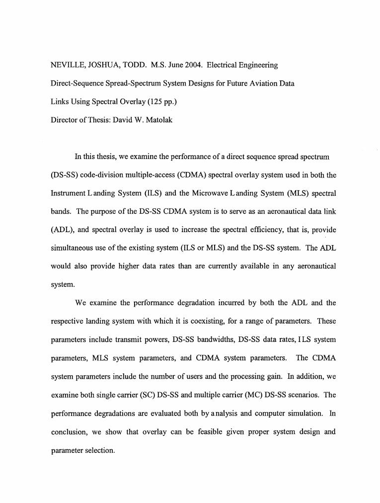
NEVILLE, JOSHUA, TODD. M.S. June 2004. Electrical Engineering
Direct-Sequence Spread-Spectrum System Designs for Future Aviation Data
Links Using Spectral Overlay (125 pp.)
Director of Thesis: David W. Matolak
In this thesis, we examine the performance of a direct sequence spread spectrum
(DS-SS) code-division multiple-access (CDMA) spectral overlay system used in both the
Instrument Landing System (ILS) and the Microwave Landing System (MLS) spectral
bands. The purpose of the DS-SS CDMA system is to serve as an aeronautical data link
(ADL), and spectral overlay is used to increase the spectral efficiency, that is, provide
simultaneous use of the existing system (ILS or MLS) and the DS-SS system. The ADL
would also provide higher data rates than are currently available in any aeronautical
system.
We examine the performance degradation incurred by both the ADL and the
respective landing system with which it is coexisting, for a range of parameters. These
parameters include transmit powers, DS-SS bandwidths, DS-SS data rates, ILS system
parameters, MLS system parameters, and CDMA system parameters. The CDMA
system parameters include the number of users and the processing gain. In addition, we
examine both single carrier (SC) DS-SS and multiple carrier (MC) DS-SS scenarios. The
performance degradations are evaluated both by analysis and computer simulation. In
conclusion, we show that overlay can be feasible given proper system design and
parameter selection.