DIGITAL SIGNAL PROCESSING FOR SEISMIC INVERSE PROBLEM
by
KAI-CHIH JOHN YUAN MS
A THESIS
IN
ELECTRICAL ENGINEERING
S u b m i t t e d t o t h e J r a d u a t e F a c u l t y of T e x a s Tech ( J n i v e r s i t y i n
P a r t i a l F u l f i l l m e n t o f t h e R e q u i r e m e n t s f o r
t h e D e g r e e of
MASTER OF SCIENCE IN
ELECTRICAL ENGINEERING
Approved
A c c e p t e d
Kay 1983
T i^^^V C^^p^ - AC KN OWL E DG EM ENTS
I an deeply indebted to Dr- John Murray for his
direction of this thesis and to the other numbers of my
committee Dr- D- Gustafson and Dr E Emre for their
helpful criticism I would like to express thanks to my
wife for her constant encouragement and patience throughout
this study
11
COITEMTS
CHAPTER E^aS
I INTROOaCTION 1
II DISCRETE SEISMIC INVERSE PROBLEM 3
Introduction bull bull bull bull bull bull bull bull bull bull - 3 The particular form of states bull bull - bull bull - 1 3 Relationship between (J j ) ^^^ ( jlraquo j1 ) bull bull bull ^ Estimation and detection bull - bull bull bull bull bull - bull 1 5
(1) Maximum likelihood estimation - bull 15 (2) Cepstrum detection - - - bull bull bull bull bull bull 1 9
Algor i thms bull bull bull bull bull bull bull bull bull 2 8 S i m u l a t i o n and r e s u l t s bull bull bull bull bull bull bull bull bull bull bull 3 3
(1) To g e n e r a t e a s y n t h e t i c se isnogram bull bull 33 (2) Implementat ion of a l g o r i t h m s bull bull 35
Comparis ion wi th H a b i b i - A s h r a f i work bull bull bull bull bull bull 6 9
I I I ^ CONTINUOOS SEISMIC INVERSE PROBLEM bull bull bull bull bull bull 72
I n t r o d u c t i o n bull bull bull bull bull bull bull bull bull bull bull bull 7 2 Trans format ion bull - bull bull bull bull bull bull bull bull 7 3 Cont inuous i n v e r s e - s c a t t e r i n g problem bull bull bull - - 75 Numerical s o l u t i o n and s i m u l a t i o n r e s u l t s - - 82 A v e r y f a s t a lgor i thm t o i n v e r t the G e l f a n d -
L e v i t a n matrix bull bull bull bull bull bull bull bull bull 117 (1) S t a t e c h a r a c t e r i s t i c s f o r Goupi l laad
l a y e r e d medium bull bull bull bull 118 (2) R e l a t i o n s h i p between r e f l e c t i o a impul se
r e s p o n s e and ( n z) G n z ) ) bull bull bull 123 (3) To compute t h e r e f l e c t i o n c o e f f i c i e n t s
from R (z) and F(n 2 ) - bull 125 (4) Convers ion formula f o r P ( i z ) and G ( i z ) 1 2 d (5) The f a s t a l g o r i t h m t o i n v e r t t h e G e l f a n d -
L e v i t a n matrix bull bull bull bull bull bull bull 133 (6) R e l a t i o n t o Robinsonraquos work bull bull bull bull bull bull 141
IV ANALOGY BETWEEN DISCRETE AND CONTINOOS INVERSE PROBLEM bull 144
I n t r o d u c t i o n bull - bull bull 144 Prom c o n t i n o u s i n v e r s e problem to d i s c r e t e
i n v e r s e problem bull bull bull - - - 144
1 1 1
-raquowlaquo v- - wI T= i n v e r s e problem t o continuous i n v e r s e problem 151
T CONCLDSION bull bull 156
I
BIBLIOGRAPHY bull - bull bull bull bull bull bull bull - - I59
APPENDIX bull bull bull 162
17
LIST OF PIGUBES
Figure Q13sect
1 An i d e a l i z e d K-layer earth system bull bull bull 4
2 The d e f i n i t i o n of s t a t e s bull laquo bull bull bull bull bull bull bull 5
3 The r e f l e c t e d and transmitted wave at the i n t e r f a c e J 7
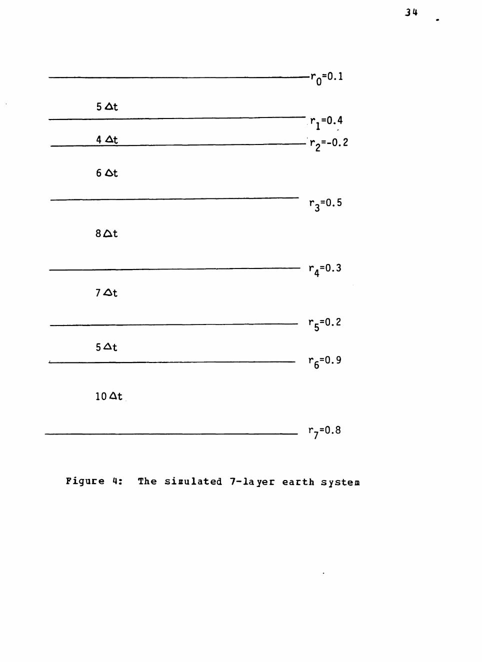
4 The s imulated 7 - layer earth system bull bull bull bull bull 3 4
5m The impulse response of the 7 - layer system (fig^ 4) 4 1
5 The r e f l e c t o r s e r i e s of l ayer 7 with no n o i s e
corruption bull bull bull bull bull bull 4 1
7 The cepstrum of f i g 6 with weighting a=0-96 bull bull 42
ampbull The n o i s y impulse response with no i se =0^000001 bull 42
9 The r e f l e c t o r s e r i e s of layer 7 with noise
d^=0000001 43
10 The cepstrum of f i g 9 with weighting a = 0 96 43
11 The no i sy impulse response of the system ( f i g 4 ) with noise (7^^=0000001 46
12 The r e f l e c t o r s e r i e s of layer 7 with noisa 0^=0000001 46
13 The cepstrum of f i g 12 with weighting a = 096 47
14- The no i sy impulse response of the s y s t e m ( f i g 4 ) with noise 0^=00001 47
15 The r e f l e c t o r s e r i e s of l ayer 7 with noisa cgt =00001-48
16 The cepstrum of f ig 15 with weighting a = 096 48
17 The r e f l e c t i o n seismogram of f i g 4 with no noise cor rupt ion 5 1
18 The inpu t s i g n a t u r e to the system in f ig 4 to genera te the seismogram S I
19 The r e f l e c t o r s e r i e s of l aye r 7 with no noise
cor rupt ion 5 2
20 The cepstrum of f ig 19 with weighting a = 096 52
21- The noisy r e f l e c t i o n seismogram of f i g 4 rfith noise Q^ = 0 0 0 0 0 0 1 53
22- The reflector series of layer 7 with noise ^^=0000001 53
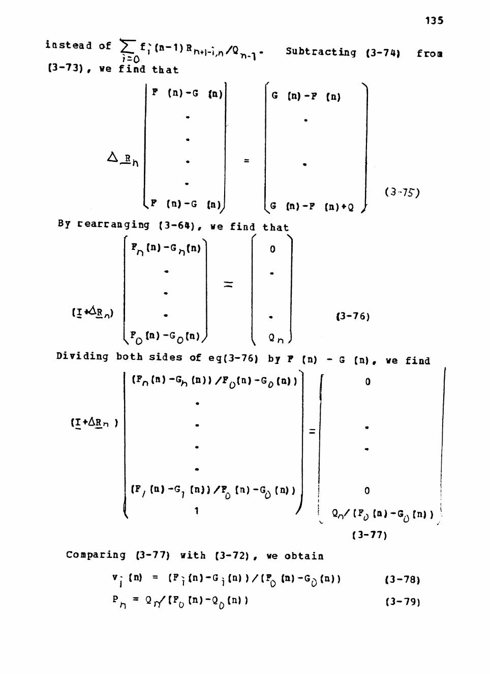
23- The cepstrum of fig22 with weighting a = 096 54
24 The noisy reflection seismogram of fig4 with noise ^i=000001 54
25- The reflector series of layer 7 with noise ^1 =000001 57
26 The cepstrum of f ig 25 with weighting a = 096 57
27 The noisy r e f l e c t i o n seismogram with n o i s e O =0-000158
28 The r e f l e c t o r s e r i e s of l ayer 7 with noisaO =0 0001 58
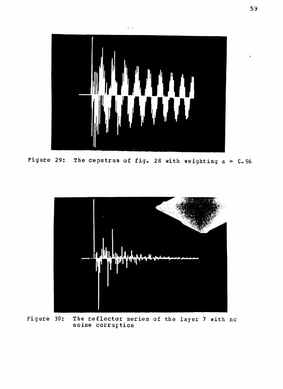
29 The cepstrum of f i g 28 with weighting a = 096 - 59
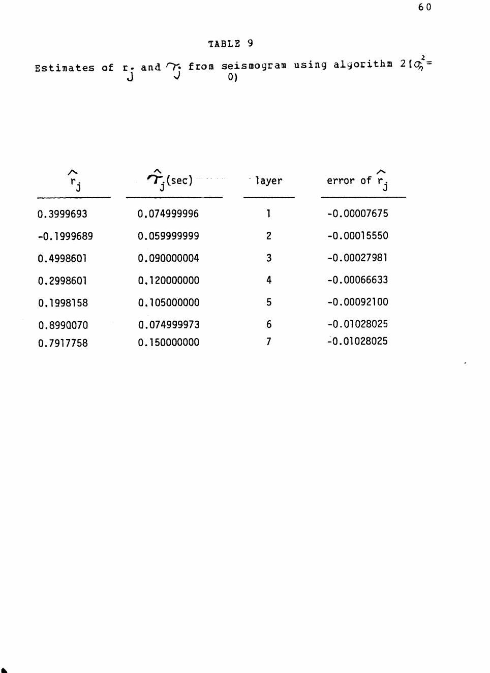
30 The r e f l e c t o r s e r i e s of l ayer 7 with no noise cor rupt ion 5 9
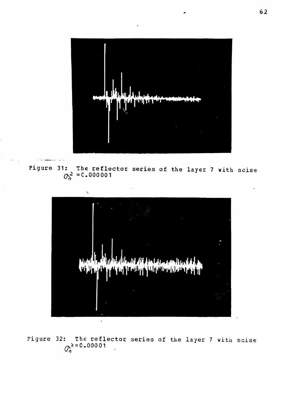
31 The r e f l e c t o r s e r i e s of layer 7 with noise O ^ = 0 0 0 0 0 0 1 62
32 The r e f l e c t o r s e r i e s of layer 7 with noiss
Qv^=000001 o2
33 The reflector series of layer 7 with noisa (gt =0000165
34 The cepstrum of the synthetic seismogram of the system fig4 68
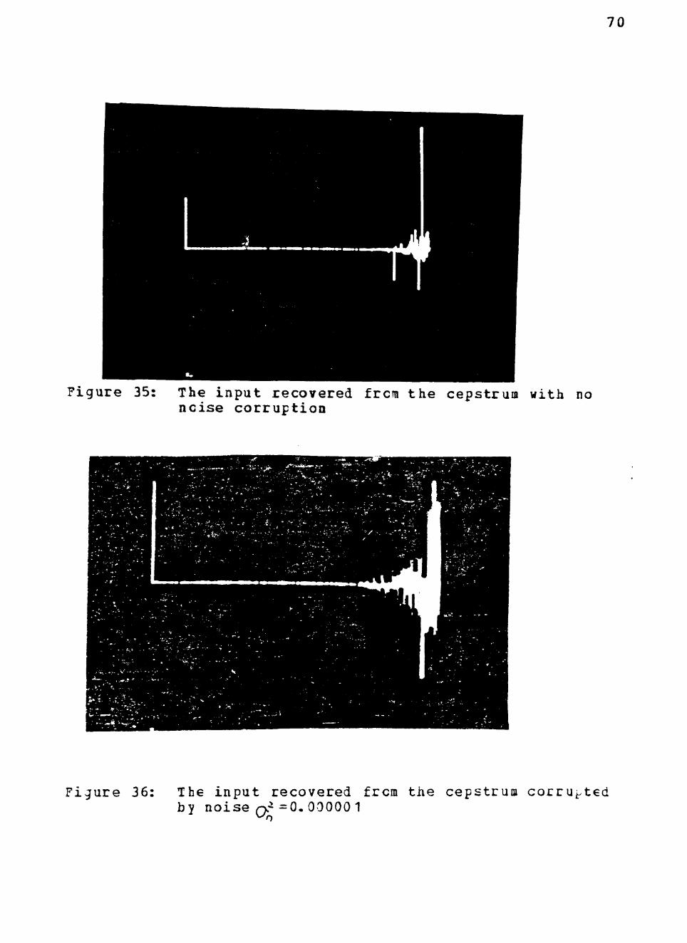
35 The inpu t recovered from the cepstrum with no noise cor rupt ion 7 0
V I
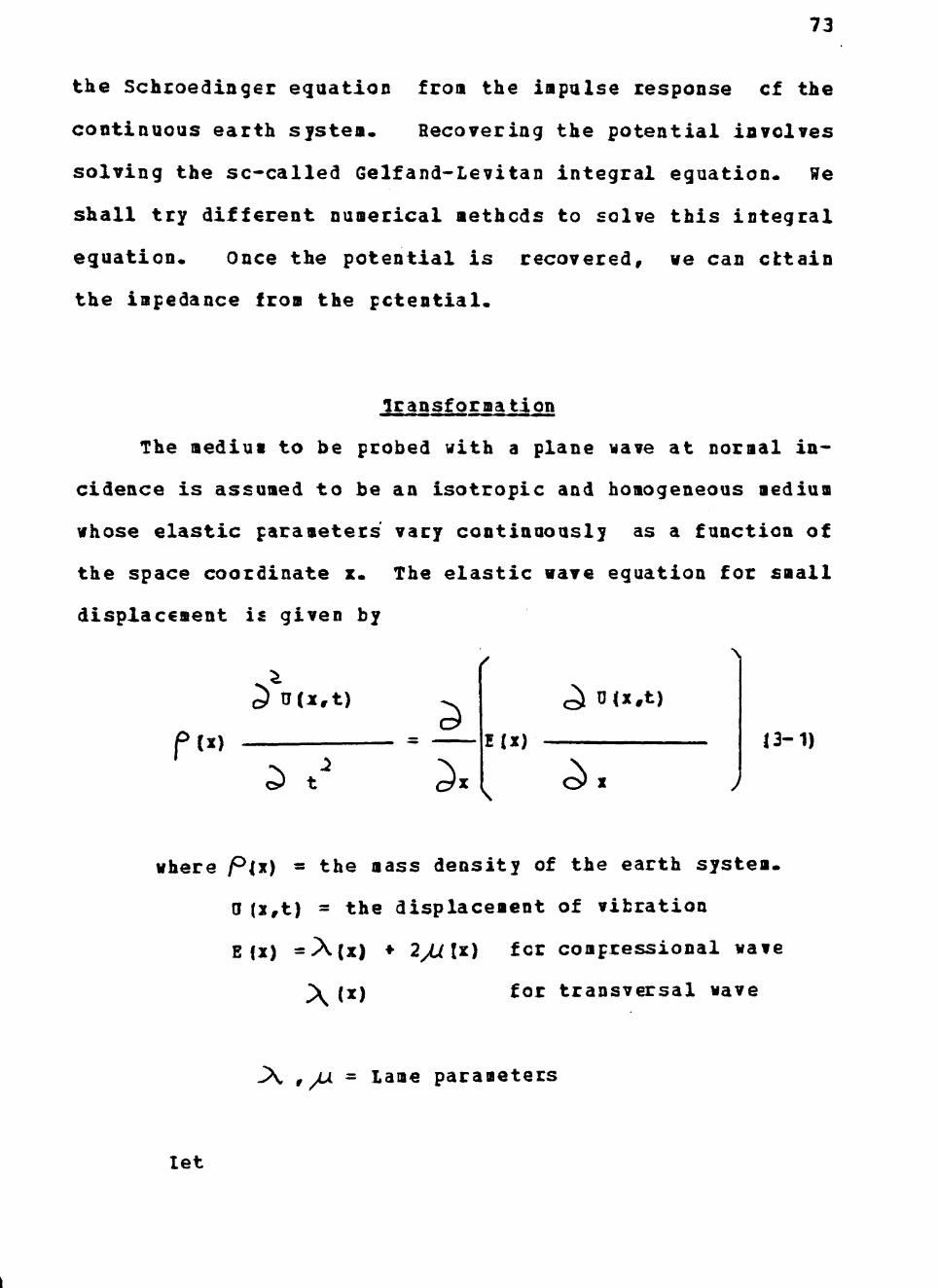
36 The input recovered from the cepstrum corrupted by no i se o =0^000001 70
37^ The input recovered from the cepstrum corrupted by n o i s e o^ =0^ 00001 bull bull bull 7 1
38 The input Recovered from the cepstrum corrupted by noise (7 =0^0001 71
39^ The medium used for illustration of inverse s c a t t e r i n g problem bull bull bull bull bull bull bull bull bull bull bull bull bull bull 7 7
40^ The simulated earth model with continuous impedance 96
41^ The impulse response of the system in fig40 with no n o i s e corrupton bull bull bull bull bull bull bull bull bull bull bull bull bull bull bull bull bull 9 7
42^ The Noisy impulse response of the system in fiq^40( O^ =0^000001) 97
43^ The noisy impulse response of the system in fi7^40( CN^=0^00001) 98
44^ The noisy impulse response of the system in fig40(
O^ =0^000 1) 98
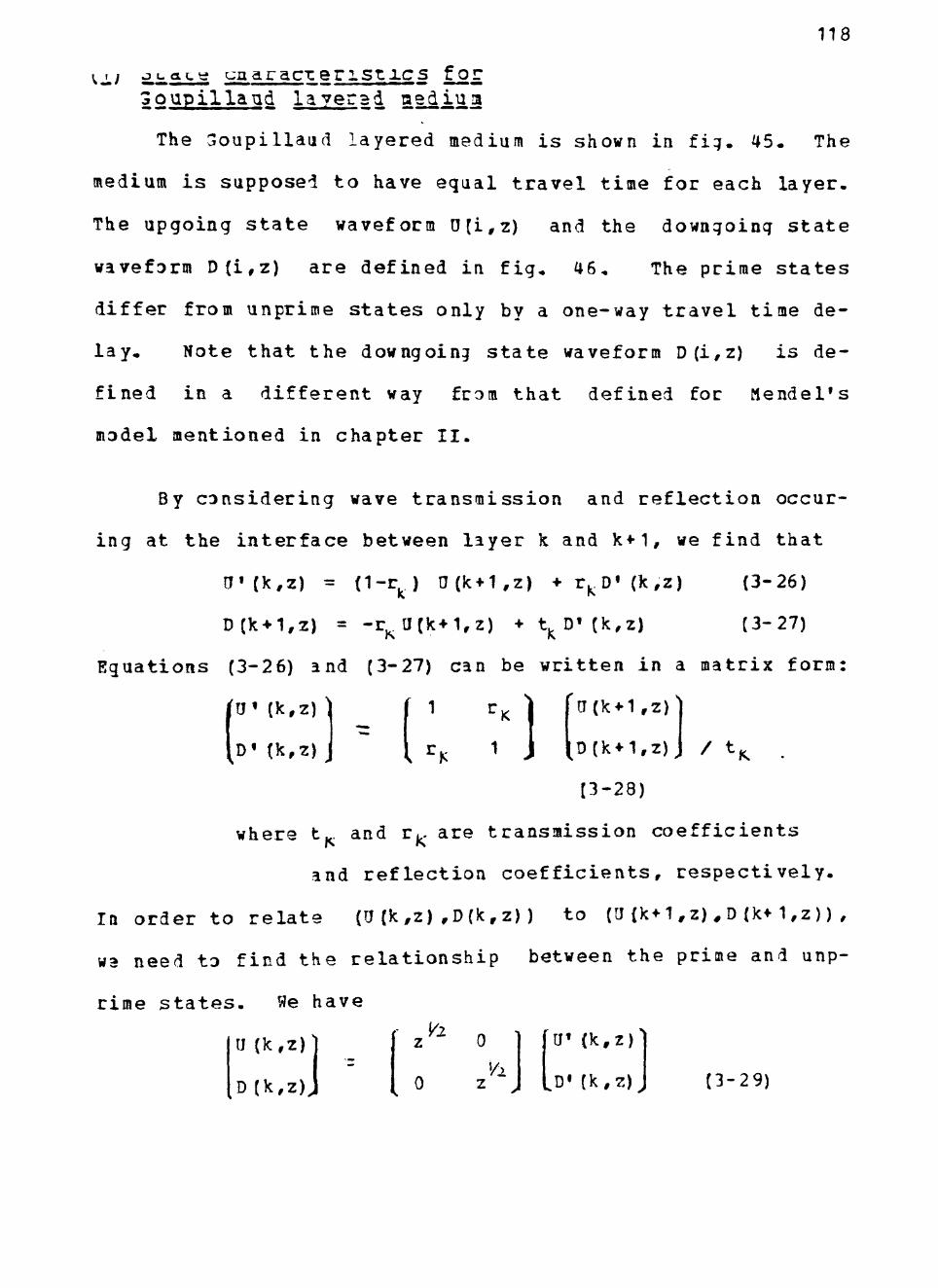
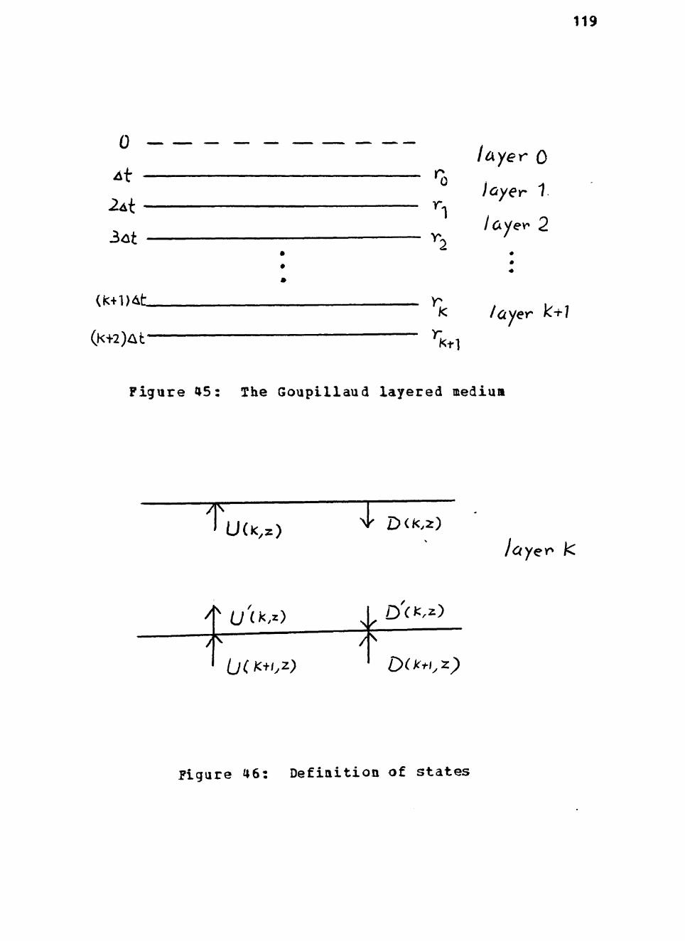
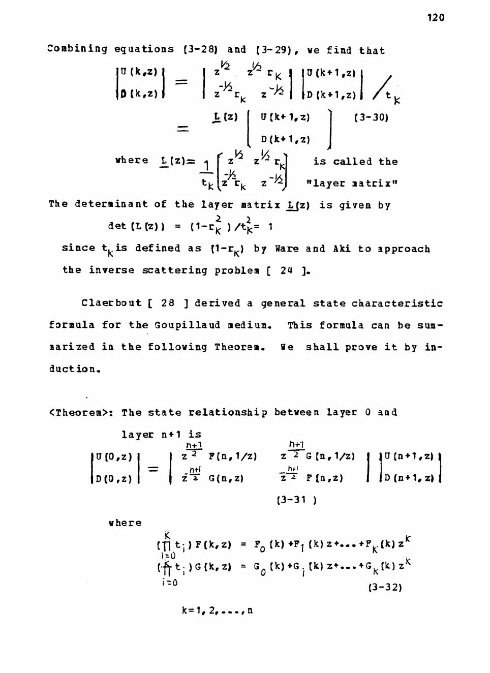
45 The Goupillaud layered medium bull bull bull bull bull bull bull bull 119
45^ D e f i n i t i o n of s t a t e s bull bull bull bull bull bull bull bull bull bull 119
47^ The d i s c r e t i z e d continuous system bull 146
48 The impulse response of the 1- layer system in f i g 47 152
49 The smoothed curve of f i g 4 5 using polynomial i n t e r p o l a t i o n bull bull bull bull bull bull bull bull bull bull bull bull bull bull 152
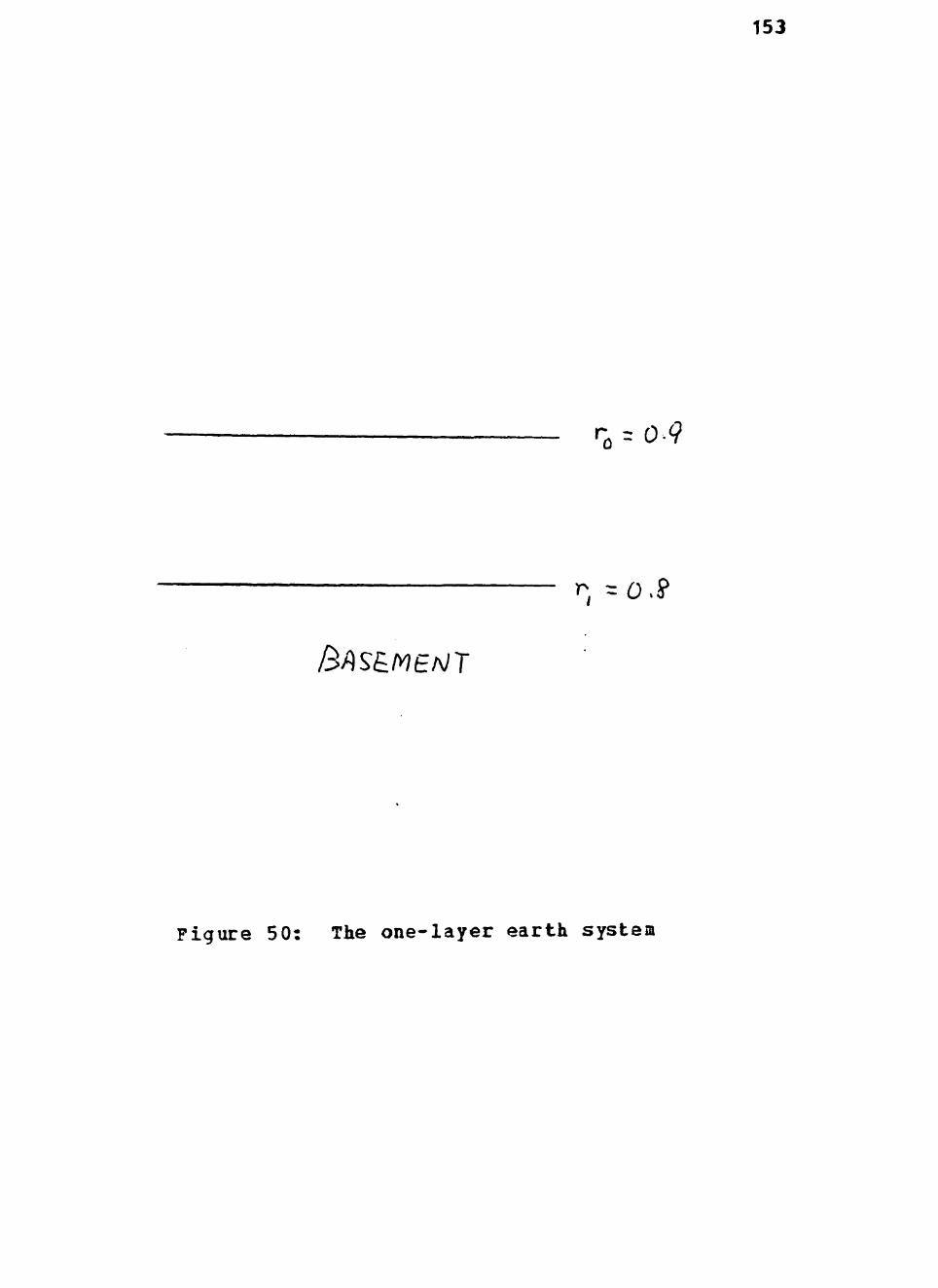
50 The one- layer earth system bull bull bull bull 153
V l l
LIST OF TABLES
Table
1
2
3
4
6
7
8
10
1 1 -
12
13
E s t i m a t e s of r ^ and 9 l us ing a lgor i thm 1 O = 0 ) - 39
E s t i m a t e s of r^ and O us ing a l g o r i t h m 1 Q = 0 0 0 0 0 0 1 ) bull bull 40
E s t i m a t e s of r and ^ us ing a lgor i thm 1 ( ^^=000001) - 44
Estimates of r and O using algorithm 1 ( Qs =00001) 45
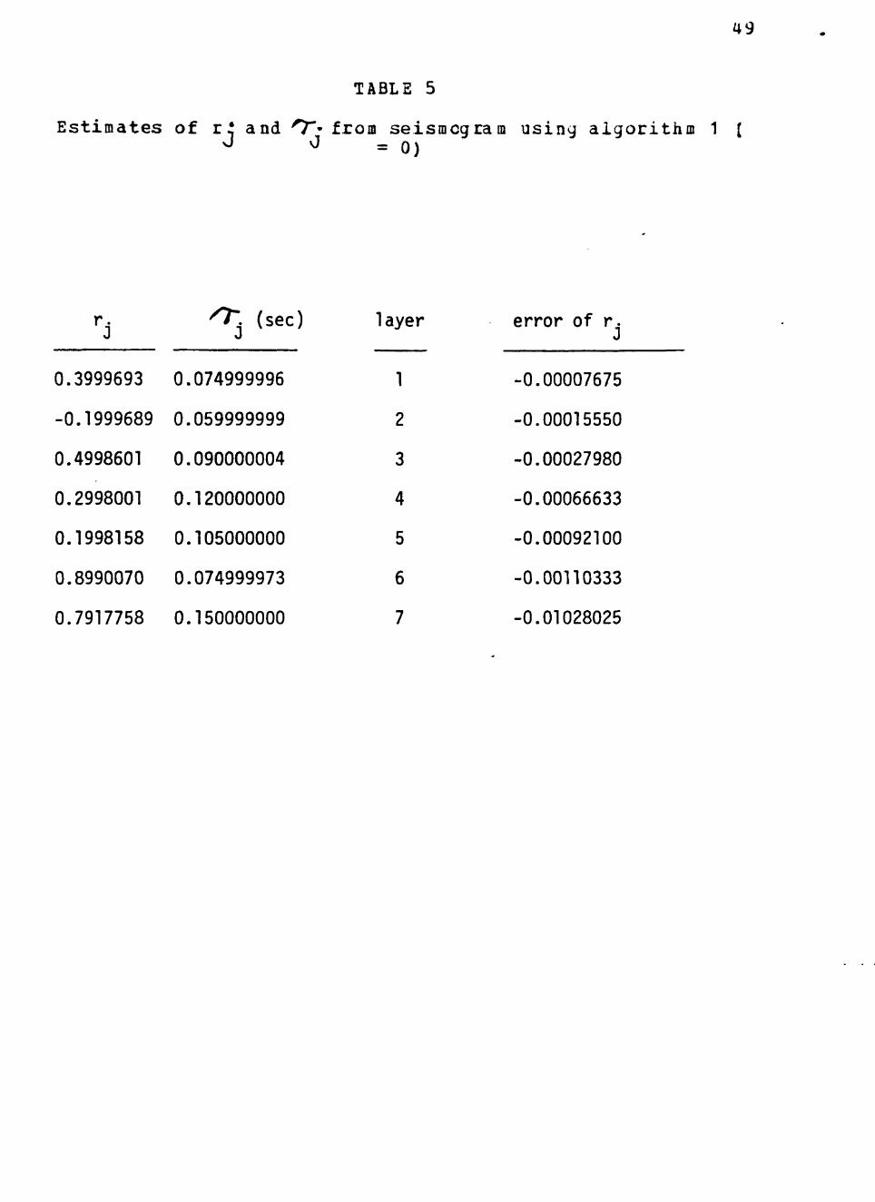
E s t i m a t e s of r j and O- from seismogram us ing a lgo r i thm 1 ^ = 0) 49
E s t i m a t e s of r^ and ^^- from seismogram us ing a l g o r i t h m Tc(7^=0000001) 50
E s t i m a t e s of r j and ^ from seismogram using a l g o r i t h m 1 (o^ =000001) 55
E s t i m a t e s of r j and O - from seismogram using a lgo r i t hm 1 Q =0000 1) 56
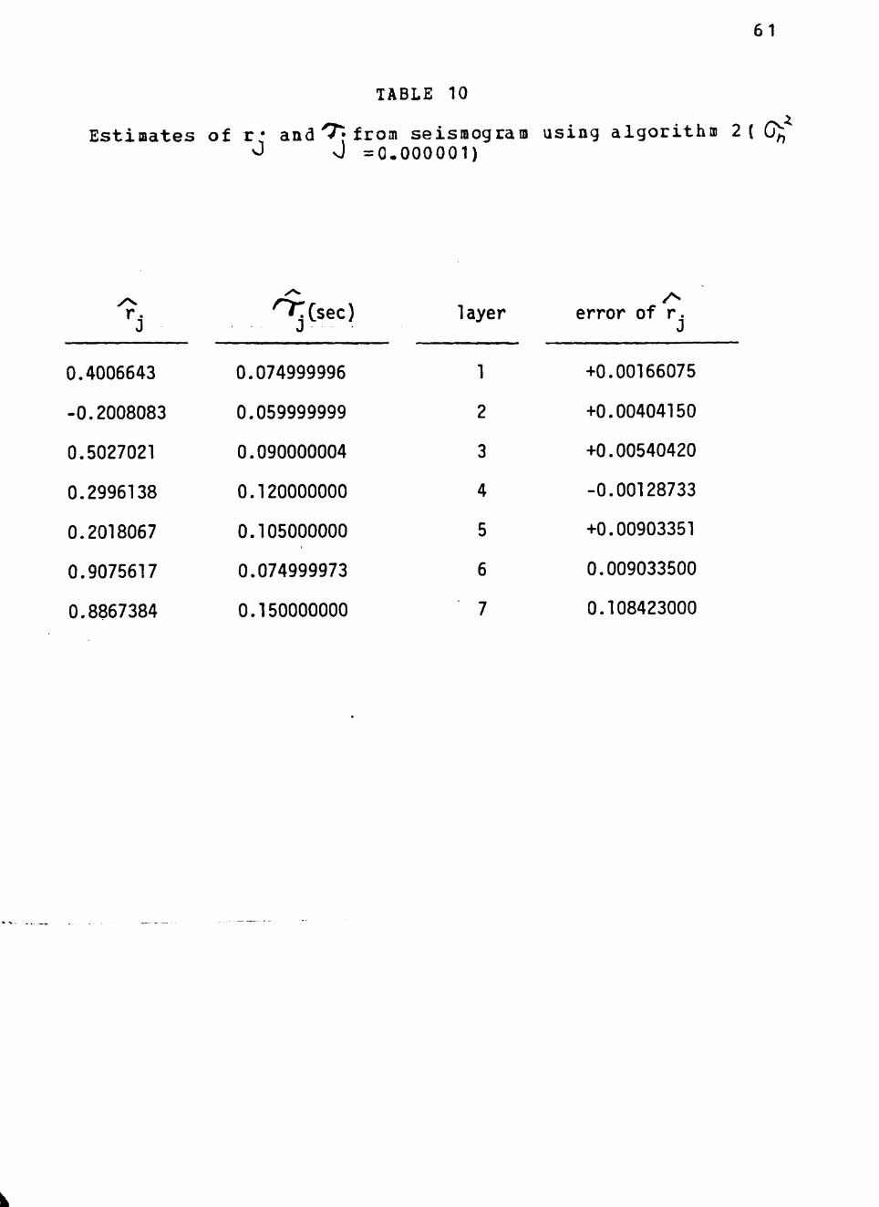
E s t i m a t e s of r j and O - from seismogram using a lgo r i t hm 2 ((7^= 0) 60
E s t i m a t e s of r j a n d ^ from seismogram using a l g o r i t h m 2 ( ^ = 0-000001) 61
E s t i m a t e s of r j and O^-from seismogram using a l g o r i t h m 2(^^=000001) 63
E s t i m a t e s of r j and yfrom seismogram us inq a l g o r i t h m 2 ( Q = 0 0 0 0 1 ) 64
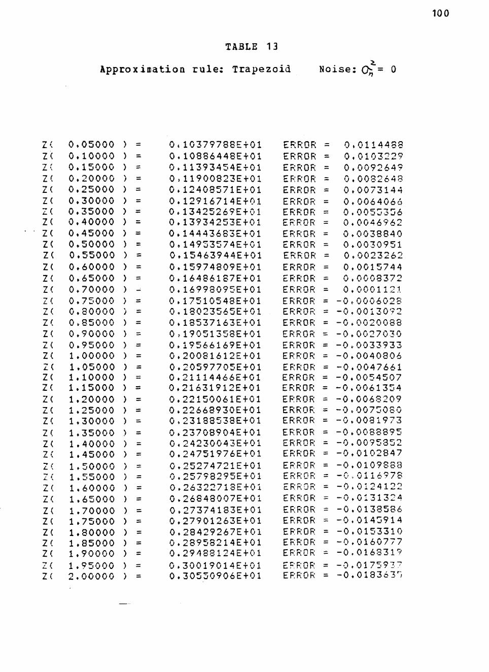
a Approximation r u l e Trapezoid Noise 5 ^ = 0 99
V i l l
T Approximation r u l e Trapezoid No i se ^ =0-000001 00
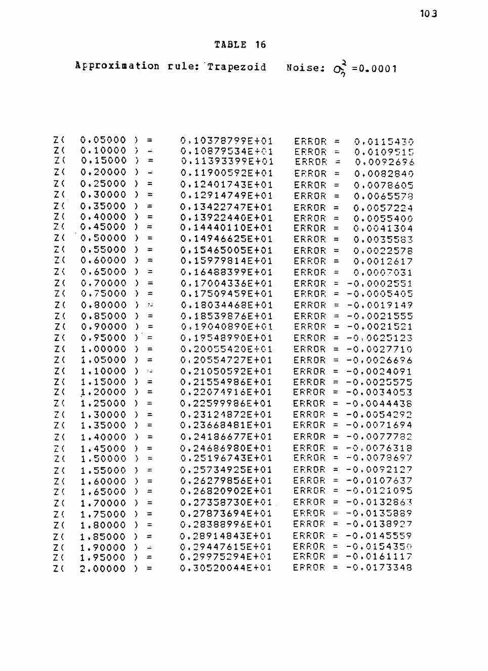
15 Approximation r u l e Trapezoid Noise gt =000001 10 1
16- Approximation r u l e Trapezoid Noise O =00001 102
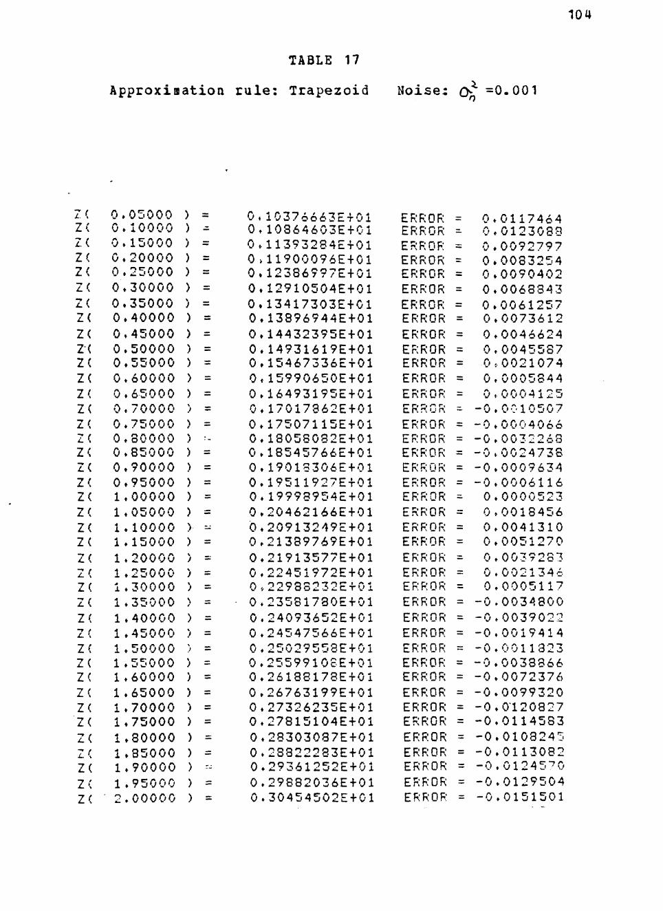
17 Approximation r u l e Trapezoid Noi s e O =0001 bull 103
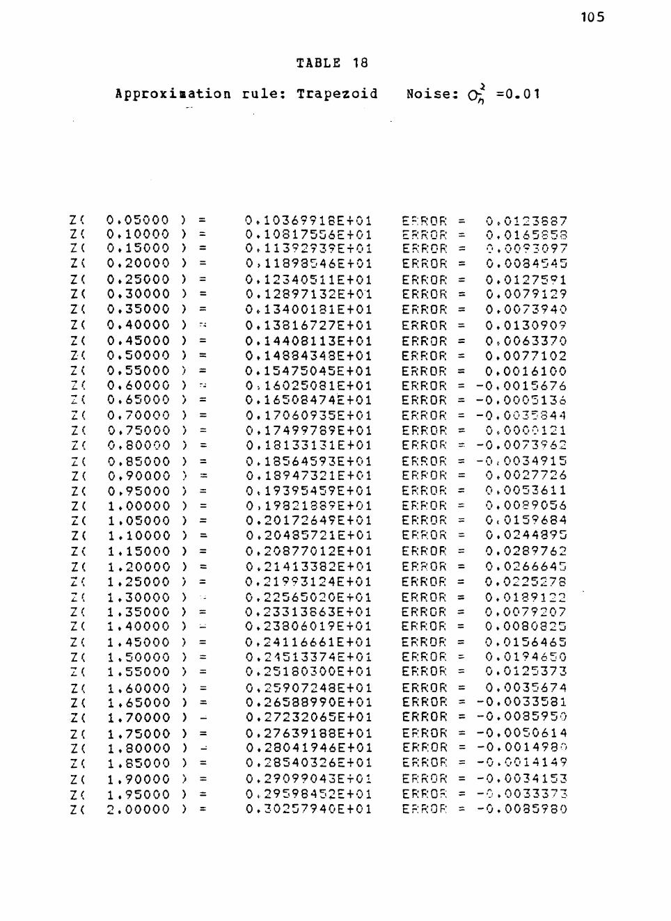
18 Approximation r u l e Trapezoid Noi s e 0^ =001 - 104
19 Approx r u l e s Trapezoid and Simpson 13 No i se 0^^=0000001 105
20 Approx r u l e s Trapezoid and Simpson 13 No i se 0^^=0-000001 - 106
2 1 Approx r u l e s Trapezoid and Simpson 13 Noise Q^i=000001 - - 107
22- Approx r u l e s Trapezoid and Simpson 13 Noise 0^1=00001 108
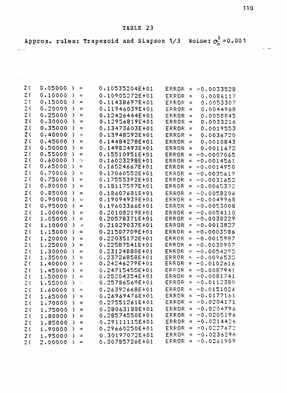
2 3 Approx r u l e s Trapezoid and Simpson 13 Noise 0^1=0^00 1 109
24 Approx r u l e s Trapezoid and Simpson 13 Noise ^ 1 = 0 0 1 110
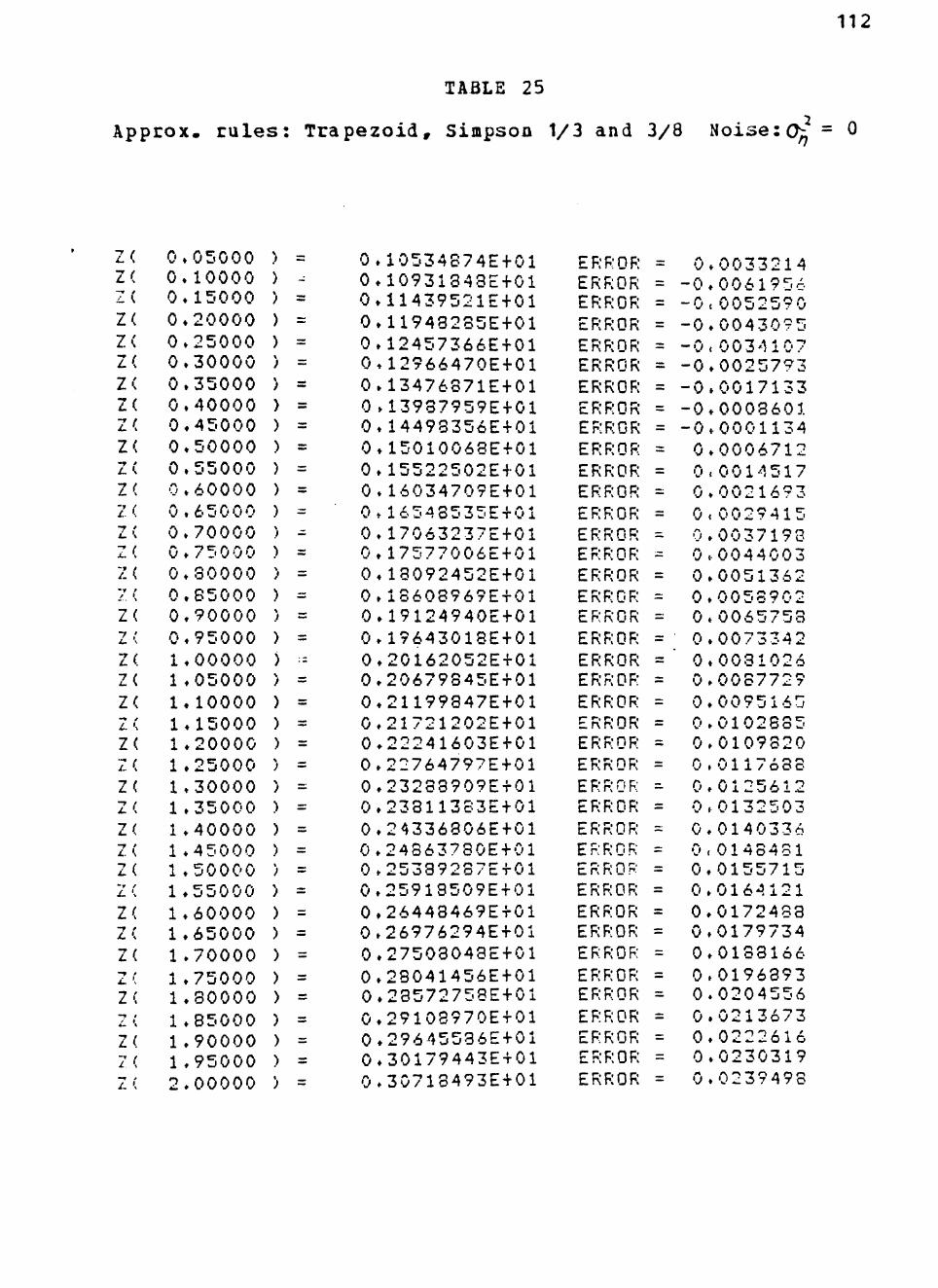
25- Approx r u l e s Trapezo id Simpson 13 and 38 Noise ^= 0 I l l
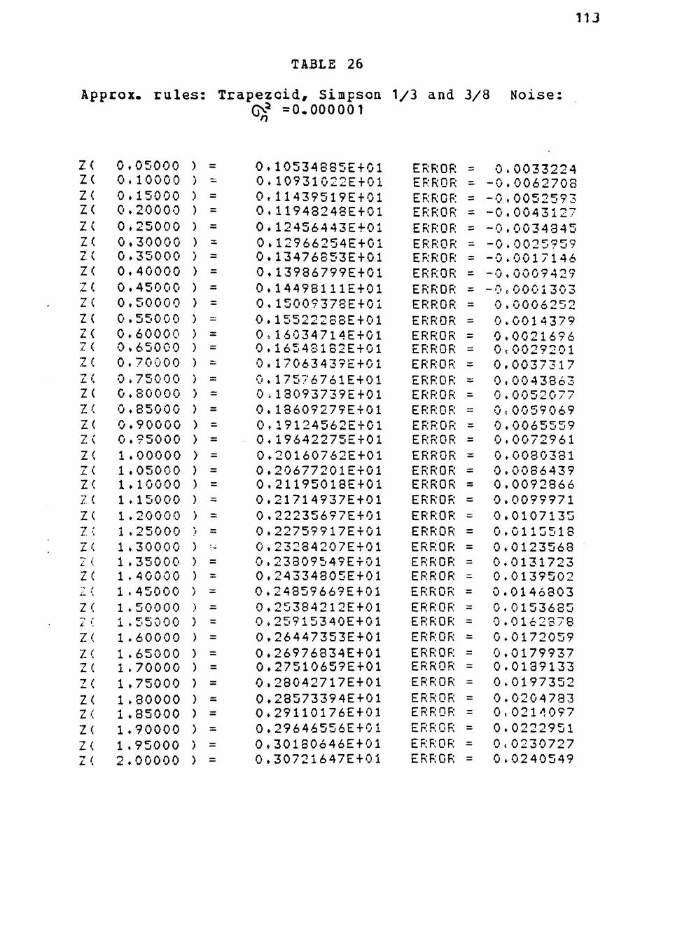
26- Approx r u l e s Trapezo id Simpson 13 and 38 Noiseok^ =0000001 - 112
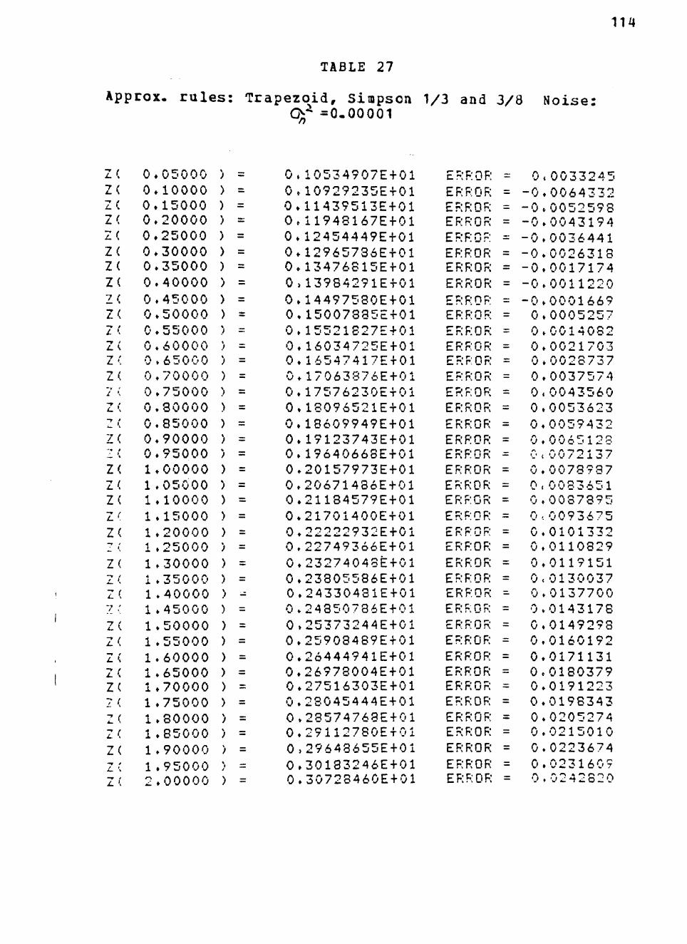
27 Approx r u l e s Trapezo id Simpson 13 and 38 ~ N o i s e ^ i = 000001 113
28 Approx r u l e s Trapezo id Simpson 13 and 38 N o i s e 0^=00001 bull - 114
29 Approx r u l e s Trapezo id Simpson 13 and 3B N o i s e 0^ = 0 001 115
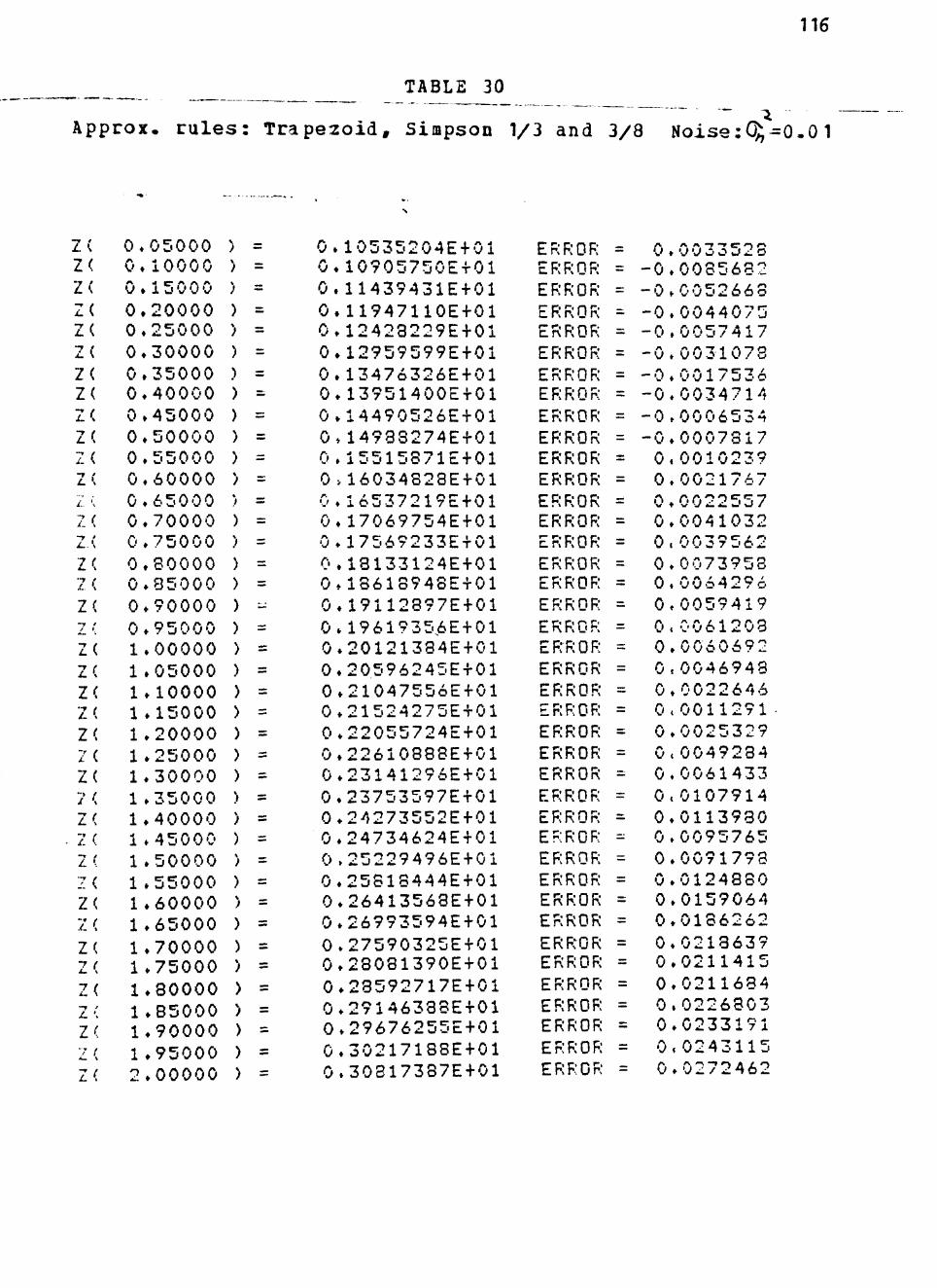
30 Approx r u l e s Trapezo id Simpson 13 and 38 N o i s e 0^=001 116
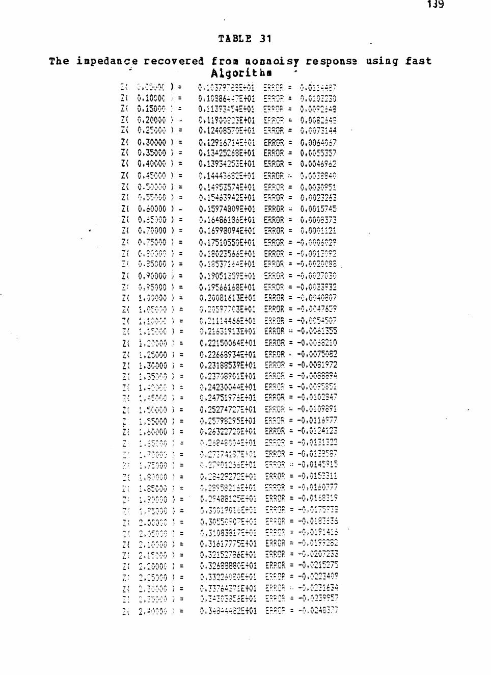
3 1 The impedance recovered from nonnoisy response us ing fas t a l g o r i t h m 141
32 The impedance recovered from noisy response ( O = 001) using f a s t a l g o r i t h m 142
I X
33 Est imates of r j for the d i s c r e t i z e d continuous system with At = 005 151
34 Est imates of r j for the d i s c r e t i z e d continuous system with At = 0005 sec 152
35- The impedances recovered from the smoothed impulse response ( f ig 46) 156
CHAPTER I
IHTHODOCTIOI
The recent advances in integrated circuit and high
speed digital computers have fostered the development of inshy
creasingly sophisticated signal processing algorithms with
reasonable cost- Digital signal processing thus plays imshy
portant roles in diverse science and engineering fields
such as acoustic sonar radar biomedical engineering
speech communication image processing seismic exploration
and many others [ 1 ]- In this thesis a particular seismic
problem mdash the seismic inverse problem mdash has been selected
and necessary digital signal processing algorithms as well
as numerical methods are used to deal with this problem-
The seismic inverse problem draws its name from the
fact that it identifies the unknown seismic system given
both the input and output- The inverse problem is known as
the identification problem in system theory Basically
system identification encompasses three major problems moshy
deling and mathematical representation estimation and vashy
lidation of the model [ 2 ] This thesis presents an apshy
proach to the seismic inverse problem by first discussing
the modeling and mathematical representation of this prob-
problem then selecting an appropriate estimation scheme
and finally discussing its validity Two different types of
seismic systems are analyzed in this thesis these arc the
discrete earth system and the continuous earth system The
approaches tc inverse problems for the discrete and
continuous system are given in cha(ters II and IJl
respectively The discussion of their analogy^ is given in
chapter If
The digital signal processing algorithms used to solve
the seismic irverse problem have teen programmed in FORTRAN
and are run on a TAI11780 computer system A display
system - COMTAI vision one20 image processing system - has
been used with the VAX11780 system to display images of
desired digital signals The PORTRAH programs used to
implement regnired algorithms are also listed in the
appendii
CBAPTEB II
CISCBETI SIISHIC IBVEBSE PBOBIEH
Introduction
The discrete seismic inverse problem in oar work is deshy
fined as an inverse problem associated with a discrete seshy
ismic system ie the layered earth system^ The discrete
earth system here is not necessary egually discretized^ In
other words the layered earth system may not have egually
spaced layers^ An idealized layered earth system as shewn
in fig^l has teen selected and its state-space representashy
tion will be developed^ The starting point for our developshy
ment is the assumption that wave motion in each lajer is
characterized by two signals travelling in opposite direc-
tions^ The functions u(t and ^-(t) denote upgoiog and
downgoing waves in the layer j respectively as shown in
fig^2 In Mendels work [ 3 ] u bull (t) and d(t) are referred
to as states Since the different location of source
orand sensor leads to a different state-space model [ 3 ]
we thus assume that the locations of both source and sensor
in our case are right on the surface of the top layer^ To
derive the state-space model we first need to consider
ni(t) A
y ( t )
0
Layer 1 ( ^ )
Layer 2 ( ^ )
^ K - 1
Layer K rj- )
Basement
Figure 1 An idea l ized K-layer earth system
7K U(t)
J-1
LAYER j
d ( t )
bullj
Figure 2 The def in i t ion of s tates
the interface condition between tuo adjacent layers^ For
the purpose of illustration let us pick interface j which
is located between layer j and layer j1^ Assuming that the
earth system is nonabsorbtive and probed with a normal incishy
dent plane wave we can find the interface equation by inshy
cluding the physical parameters of the layer j ie^ the reshy
flection coefficient r and the transmission coefficiett t ^
This fact is sketched in figlaquo3 where we draw ray diagrams
with tile displacement along the horizontal axis so that
rays appear to be at ncnnormal incidence and so do not overshy
lap one another^ The interface eguation of the interface j
is
Dpgoing jt ) = j jf ) J C)
= rjd^tt) bull ( 1 - rj ) u(t) J2-1)
Downgoing ^jbdquott^^) = tjdj (t) 4 (-rj) uj(t)
= I 1 bull r j ) djCt) - jgti gt ^2-2)
Be have used the fact that t = 1 bull r for the normal incishy
dence case Assuming the earth sjtem has K layers and the
transmitted wave goes down to the layer K l without any reshy
turn i e n |Ct) - 0 we obtain the state space model by
noting ^Q I ) gt () r where m(t) is the input of the system
u (tOi) = r^d^(t) bull ( 1 - r ) u^Jt) 2-3a)
d^it-^) = ( 1 bull r^) m(t) - rQUgt(t) (2-3b)
u (t^) = r d (t) bull ( 1 - r ) u Jt) (2-3c)
d (t+7^) = ( 1 bull rjj) dj(t) - rj uj(t) (2-3d)
J = 23 bull Kmdash1
Figure 3 The reflected and transmitted lave at the interface j
8
tt)lt(tOj) = rc^KJ ^2-3e)
d^Ct^O = ( 1 bull rj ) d^^(t) - r^^^n^ lt) | 2 -3 f )
To obta in the output equat ion we cons ider the
i n t e r f a c e cond i t ion on the surface of the top l a y e r i t s
I n t e r f a c e equation i s given fay
y ( t ) = r ^ - t t ) bull ( I - E Q ) u^Ct) (2-4)
which i s the ontput equation of the system
(2-4) and ( 2 - 3 a b c d laquo e f ) c o n s t i t n t e the s t a t e - s p a c e
model for t h e layered earth system and the i n i t i a l
c o n d i t i o n s of s t a t e s are noted as
U j ( t ) = 0
d(t) = 0 for 0 lt t lt ^ ^ (2-5)
The state space model can be reiritten in a matrix form
which gives a similar form to the state equations
encountered in system theory This fact has been justified
by Hendel et al [ 3 ] The matrix form of the state-space
model is -1 Z X (t) = A xft) bull b met) (2-6)
y(t) = c^x(t) bull i QlaquoCt) (2-7)
where
x(t) = ccKd-j (t) ^^dj^(t)u-j(t) ^^^Uj^(t))
2 = diag (z- Z2-^Zj^z-jZ2-raquof Zjj)
2 is a 0~j second delay operator)
A is a 2R by 2K sguare matrix which has the form
A = Al A2
A3 AH
Al
1
0 bull
11+r-) 0 bull
I1gtr^
bull 0
bull 0
bull 0
0
0
0
0 bull bull (Ur i
A2
A3
A4
-diag(rQr^ bull-bull rj_ )
aiag(r^r^ bullbullbull rj )
0 n-c-) 0
0 0
0
0
0
0
(l-r^)
bull 0
bull 0
0
0
bull bull laquo- icl
b = col (1rQ00 0)
10
c = col(00 bullbullbull 1-r^0 0)
K1-th element
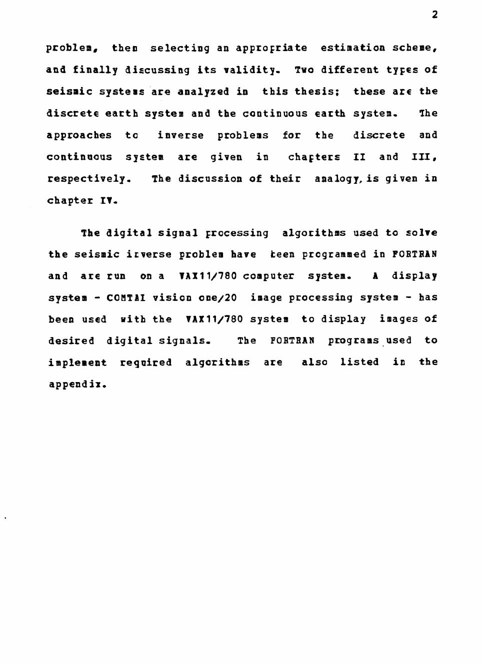
To find the transfer function we take the Fourier
transform of (2-6) and (2-7) on the unit circle (ie the
Fourier transform) and then we find
F(2 )X(ii) = A 1(40) bull b H (agt)
where
f ( ) = exp(jltdgt^)
exp C jwr^)
expljw^)
exp(j^gt^)
exp(JM^)
(2-8)
(2-9)
N
eip(jui9j^)
11
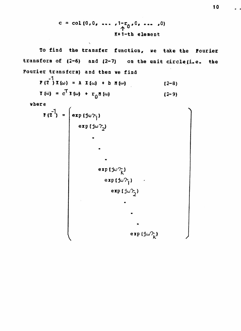
By (2-8) and (2-9) we find the transfer function
Y(iO)
1 -1 = c t F(2 ) - A ) tgt bull CQ 12-10)
HfcJ)
(2-10) suggests a conceptually straightforward procedure to
compute y(t) given the input m (t) (2-10) is useful for
theoretical purposes since the explicit calculation of
( F (2 ) - A ) is quite difficult Instead of using (2-10)
we employ a bullray tracing technique to generate y (t) - The
ray tracing technique was originally suggested by nendel [ 3
where he defined mapping rules to track hov a state
waveform propagates at an interface by observing the
state-space model (2-34) The disadvantage of Hendels ray
tracing technique is the large storage reguirement for the
state-reference table Instead of strictly following
lendels way we apply Bobinsons idea to alleviate this
problem [ 4 ] Be start to generate the synthetic
seismogram y (t) of the 1-layer case by a ray-tracing
technique and then use the relationship derived by
Robinson [ 4 ]ie
B^CZ)
^ n laquon-i^gt ^
1 bull r^H^ (2) z (2-11)
where B (z) is the 2-transform of the reflection response
for the n-layer system and r^is its reflection coefficient
12
on the surface By s e l e c t i n g n ^ 2 we can find the
r e f l e c t i o n response of the 2-Iayer case from that of the
1-layer case by (2-11) Continuing in th i s way we sha l l
find the response(the outpat of the system) for a larger
n-layer case at w i l l To obtain a noisy output(z ( t ) ) we may
add a noise source v (t) which i s a random pcocess
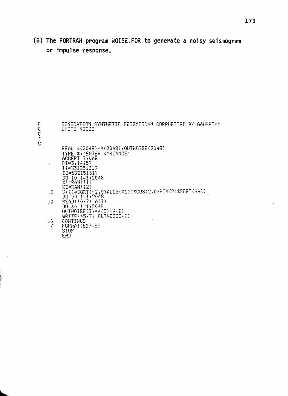
representing the no i se A FOBTBAB program NOISE i s written
to generate a white gaussian noise and i s l i s t e d in the
appendix Anstey pound 5 ] dicussed different sources of noise
and concladed that addi t ive gaussian white noise i s a f a i r l y
r e a l i s t i c assumption^ For a zero-mean gaussian white no i se
we know that
Bt v l t ) ) - 0
and
Kv(t-s) = Hv(t-s) = B( v ( t )v ( s ) ) laquo N lt^(t-3)
where Kv(t-s) and Bv (t-s) are covariance and
correlation functions of noise and ^(t-s) is the
Oirac delta function^
The output yt) or z (t) of the earth system is
geophysically called the seismogram The simulated
seismogram generated by the state-space model is called the
synthetic seistogram
13
The particular form of s ta t e s
Habibi-Ashrafi has shown that s t a t e s d (t) and u (t) of
a layered earth system described by the s tate-space model
(2-67) and i n i t i a l condition (2-5) have the fol lowing
forms [ 6 ]
laquo^(t
k=1 i K laquo ^ - JK 12-12)
1=1
t - Cj^) (2-13)
J mdash 9^0 bullbull K
The time delays DJ and Ci- satisfy the inequalities by JK bullJl
0 i 27 C- 0raquoand are ordered as
The integers Rj and Lj depend on the observation interval
A 4 and B are the amplitudes of the wavelets arriving at J Jl times D and Cj respectively Examining (2-12) and
(2-13) we see that either u(t) or d (t) is a composite
waveform which consists a number of vavelets having the same
shape as m(t) bat scaled by A raquo or B and delayed by t-
or C In the fol lowing s e c t i o n we sha l l r e la t e the in-
formaticn contained in the f i r s t wavelet(actuallyAj1 and
Dj1) to the charac ter i s t i c parameters r - andV J J
14
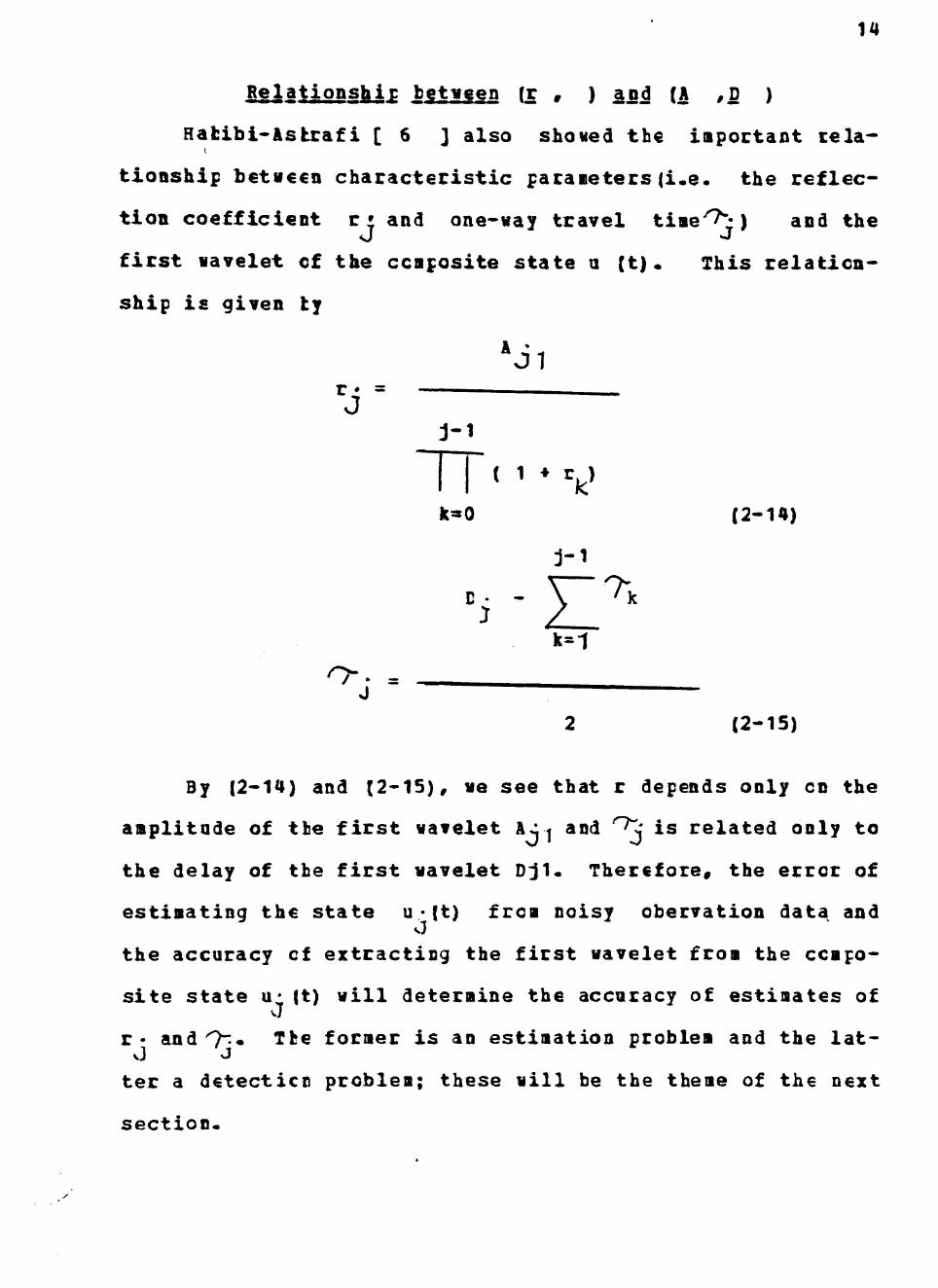
Relat ionshic between (r ) and (A D )
Habibi-Astrafi [ 6 ] also showed the important re la -
t ionship between charac ter i s t i c parameters ( i e the r e f l e c shy
t i on c o e f f i c i e n t rraquo and one-way travel t ime^M and the
f i r s t wavelet cf the composite s ta t e u ( t ) bull This r e l a t i o n shy
ship i s given ty
A Jl
J J - 1
I I (1 ^ V klaquo0 (2-14)
k=1
J (2-15)
By (2-14) and (2-15) we see that r depends only on the
amplitude of the first wavelet A^| and ^^ is related only to
the delay of the first wavelet Dji Therefore the error of
estimating the state u bull (t) from noisy obervation data and
the accuracy of extracting the first wavelet from the ccmpo-
site state u (t) will determine the accuracy of estimates of
r- and O^ Tfce former is an estimation problem and the lat-
ter a detecticc problem these will be the theme of the next
section
15
Estimation and detection
Since the obervation data are corrnpted by noise ie
2 (t) = y (t) bull ^ (t) we thus need an estimation scheme to reshy
store the required information from noisy obervations The
estimation criterion we select is maximum likelihood(HI)
pound 78 ] le do not estimate the parameters randOj dishy
rectly Instead we estimate the states xx (t) and d(t)
first and then extract the required information - ^
from the estimates of the states to estimate r bull and Or-
Examining (2-1) and (2-15) we see that the required inforshy
mation is nothing but the fixst wavelet of laquojlt)- As menshy
tioned before we need the amplitude A -j to calculate r and
th
shown in (2-12) consists of a number of closely spaced wavshy
elets In order to detect the location of the first wavelet
and estimate its amplitude we are required to solve a sigshy
nal overlapping problem^ An improved cepstrum detection
technique is exploited to deal with this problem
e delay D- tc calculateTv- The state u(t) which is
11) Maximum likelihood estimation
He begin ty observing the noisy output equation which
is given by
z(t) = y(t) bull v(t)
= rQm(t) bull (1-rj )a-|(t) bull v(t)
= y( t u^(t) ) bull v(t) (2-16)
where v (t) is assumed to be a zero mean white
oise
Observing (2-16) we know that the estimation of u-i(t) is a
problem in continuous waveform estimation and is discussed
in detail by Mahi and Trees pound78] To implement HI
estimation we need to find the likelihood function p(z(t) n
(t)) which is a conditional probability function of 2(t)
given n^(t) Since the noise v(t) is assumed to be a zero
mean white gaussian noise we have
Kv(t-s) = ir v(t)v(s) = H lt$(t-s)
where M = Variance of noise = 0^
Assuming z (t) is measured in a time interval (0 Tl) the
likelihood function can be found as pound 7 ]
I f It Pz (t) u^ (t)) - ( V T T T M ) ixpj-J J(z (t)-r bullQ V 1 m(t)-M-r)u(t))
-1 raquo Kv(t-s)(z(s)-r m(s)-(1-r^)u-jls)) dt ds
= (1JTfrN)Exp j -5 J ( z ( t ) - r ^ m ( t ) - ( 1 - r ^ ) u ^ ( t ) ) d t
0
(2-17)
Dsoally we use the log likelihood function instead of the
likelihood function (2-17) By taking logarithms on both
sides of (2-17) and discarding the constant term we find
ife(t) u^It)) = -J (z(t)-r^mt)-(1-r^)u^(t)) dt
bull^0 12-18)
Similarly the log likelihood function can be found as
17
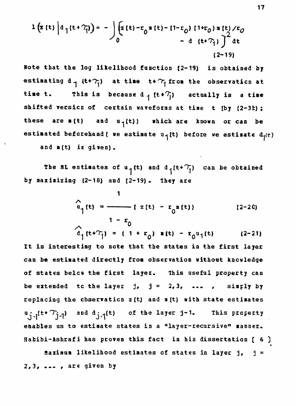
l(2Ct) |lti-|(t ))= - j |2(t)-r^m(t)-(1-r^) (Ur^)m(t)r^
0 - d (t7 ) 1 dt
(2-19)
Bote that the log likelihood function (2-13) is obtained by
estimating d- (t -T ) at time t0-^from the observaticn at
time t This is because d laquo (t) actually is a time
shifted version of certain waveforms at time t (by (2-3t)
these are m(t) and u^(t)) which are known or can be
estimated beforehand ( we estimate u-(t) before we estimate d (t)
and m (t) is given) bull
The BL estimates of u^(t) and d (t+7) can be obtained
by maximizing (2-18) and (2-19) Ihey are
1
D^(t) = ( z(t) - r^m(t)) (2-2C)
d^(t^^) ^ ( 1 bull r^) m(t) - rQU^(t) (2-21)
It is interesting to note that the states in the first layer
can be estimated directly from observation without knowledge
of states belclaquo the first layer This useful property can
be extended tc the layer j j = 23 simply by
replacing the cbservaticn z (t) and m (t) with state estimates
u- i(tTi-) and d H(t) of the layer j-1 This property
enables us to estimate states in a layer-recursive manner
Habibi-Ashrafi has proven this fact in his dissertation pound 6 3 4
Haximum likelihood estimates of states in layer j j
23 -- areuro given by
18
iit) - ( u (taj - d4^(t]) (2-22) J JI J j-i -
1 - r _
d Ct^) = ( 1 bull rj-|) dj^(t) - r Uj(t) (2-23)
Observing (2-22) and (2-23) we find the state estimates
satisfy the saie functional equations (2-3) that states of
the system satisfy The estimate of states u(t) and d (t)
is a random prccess since the observation z (t) is corrupted
by a random process v(t) which was assumed to be Gaussian
and wide sense stationary The ax state estimator is a
linear tine-icvariant operation on cbservation it follcws
that the estiiated states are also wide-sense stationary
gaussian processes^ Therefore we can cospletely described
the estimation error and the quality of the estimator by
evaluating only second order statistics ie^ mean and
covariance function of the estimation error^ Habibi-Ashrafi
has shown this fact in his dissertation^
So far we have discussed the property of NL estiaator
and necessary characteristic equations to implement HI state
estimation 7he next section will give a detection scheme
to locate the first wavelet in the upgoing state u -(t) and
extract the required information to estimate r and ^bull J J
19
12) Cepstrum jftection
Our ultiiate goal is to estimate the reflection coeffishy
cient r and the one-way travel time for each layer of
the earth system^ Egnations (2-14) and (2-15) give the reshy
lationship between characteristic parameters (r and ) and
the first wavelet of u (t)bull To compute r and we need
to determine both the amplitude and delay of the first wavshy
elet as menticned previously Examining (2-12) which is
Rj
k=1
we see that u (t) is the superposition of a number of wavshy
elets (Kj wavelets in this case actually Rj ) which are
delayed scaled replicas of m(t) Dsually these wavelets
are closely spaced and thus bring about the signal overlapshy
ping problem Several references related to solving this
problem did not give satisfactory results pound 91011 ] and
the problem is general reaains unsolved In our case we
are interested in detection of only the first wavelet and
the problem is a little simpler since we are not required to
detect every wavelet in uraquo(t) Habibi-Ashrafi pound 6 ] used a
suboptimal scheme to approach this problem by assuming a mishy
nimum space between wavelets to reduce observation ncnli-
aearity of tiwe delay in (2-12) After doing this he used
HL estimation on the modified upgoing state equation siiilar
20
to (2-12) t o find r^ and O bull This i s accomplished by two J vj
filtering scheaes namely the generalized matched filter
and the linear discrete filter pound 6 ]bull Instead of follcwing
the above procedure we shall use a modified cepstrum
technique
Historically the cepstrum has its roots in solving
deconvolntion problems of tmo or more signals The
literature regarding this is rich and varied pound 12 ] and
encompasses linear prediction predictive deconvoluticc and
inverse filtering Bainly the cepstrum is classified into
the power cepstrum and the complex cepstrum according to
different purpcse and application^ ie are interested in the
complex cepstrum since it gives informaticn about amplitude
and phase of the original signal in contrast to the power
cepstrum which gives only amplitude information pound 12 ]bull The
complex cepstrum is an outgrowth of hcmcmorphic system
theory developed by Oppenheim pound 13 ]bull The definition of the
complex cepstrom is given by
C(x(t)) = Z ( ln( X(z) ) ) (2-24)
where X(z) = the 2-transform of x(t)
Z = inverse Z-transform
In practice we implement the Z-transform on the unit circle
by using the discrete Fourier transform^ Therefore (2-24)
can be reduced to -1
C(x(t)) = F( ln( F(x(t)) ) ) (2-25)
where F and F indicate the forward Fourier transform
and inverse Fourier transform respectively
Bow let us Icck at how the cepstrum ( ve shall use the
cepstrum to represent the complex cepstrnn from now on )
helps us extract the required informaticn ie the
amplitude and delay of the first wavelet from the composite
state u (t)bull For the purpose of easily implementing
cepstrum analysis we add the input B(t) which is zero
delayed and ccit scaled to u (t) to form a new composite
state n bull (t) which is J
Kj
^j(t) = m(t) bull V A^ m(t-Dj^) (2-26)
k=1
Examining (2-2euro) we see that n (t) is sinply a composite
state of m(t) and its delayed echoes (2-26) is recognized
sinply as
Kj
u-(t) laquo Mt) M bull V Ajilt SitD^^) ) (2-27)
k=1
(2-27) can be viewed as a response of a l i n e a r system whcse
impulse response i s
k=1
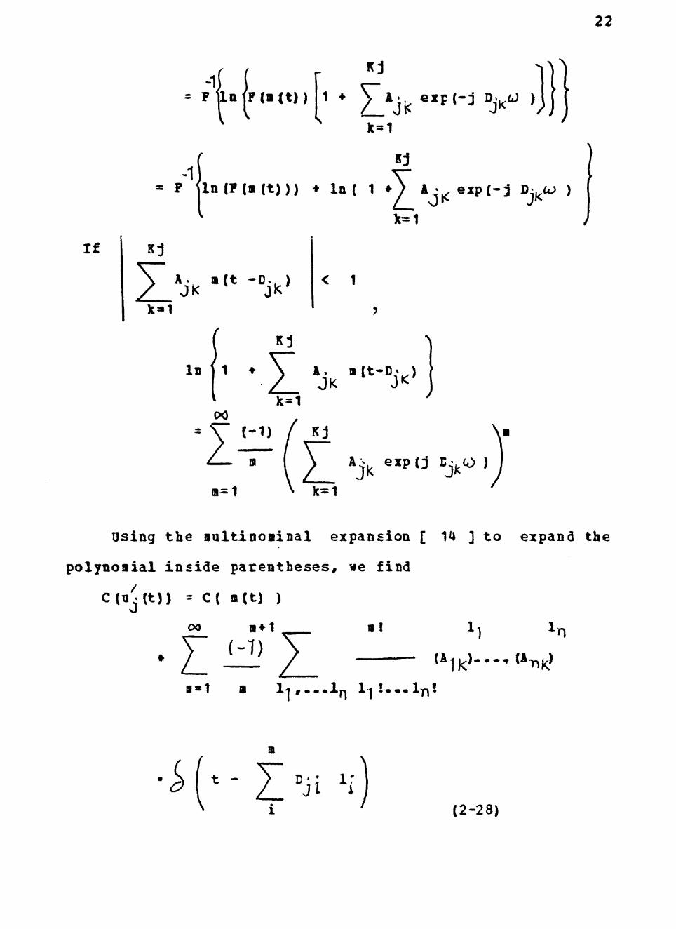
and t h e input i s g i v e n as m ( t ) Now l e t us c o n s i d e r the
cepstrum of t h i s new composite s t a t e u - ( t ) -1 ^
F t U j ( t ) ) ) )
22
If
= F lln fF (m (t))
-1
Kj
1 bull y ^^ exp(-j Dv^ )
k=1
Kj
JIC-- -y^u
laquo F ^ln(F(m(t))) bull ln( 1 bull Aj^exp(-j Dj^a )
klaquo1
Kj
A m(t -degjkgt
kraquo1
lt 1
In 1 1
oo
Kj
k^l ^
L mdash m
m=1
Kj
k=1 jk P =gtlt
Using the multinominal expansion pound 14 ] to expand the
polynomial inside parentheses we find
C(Uj(t)) = C( m(t) )
OQ m1
(-1) I I ml bulln
- (A^l^) (A )
11 m If^^sin li bull laquobull ifbull
m
(2-28)
23
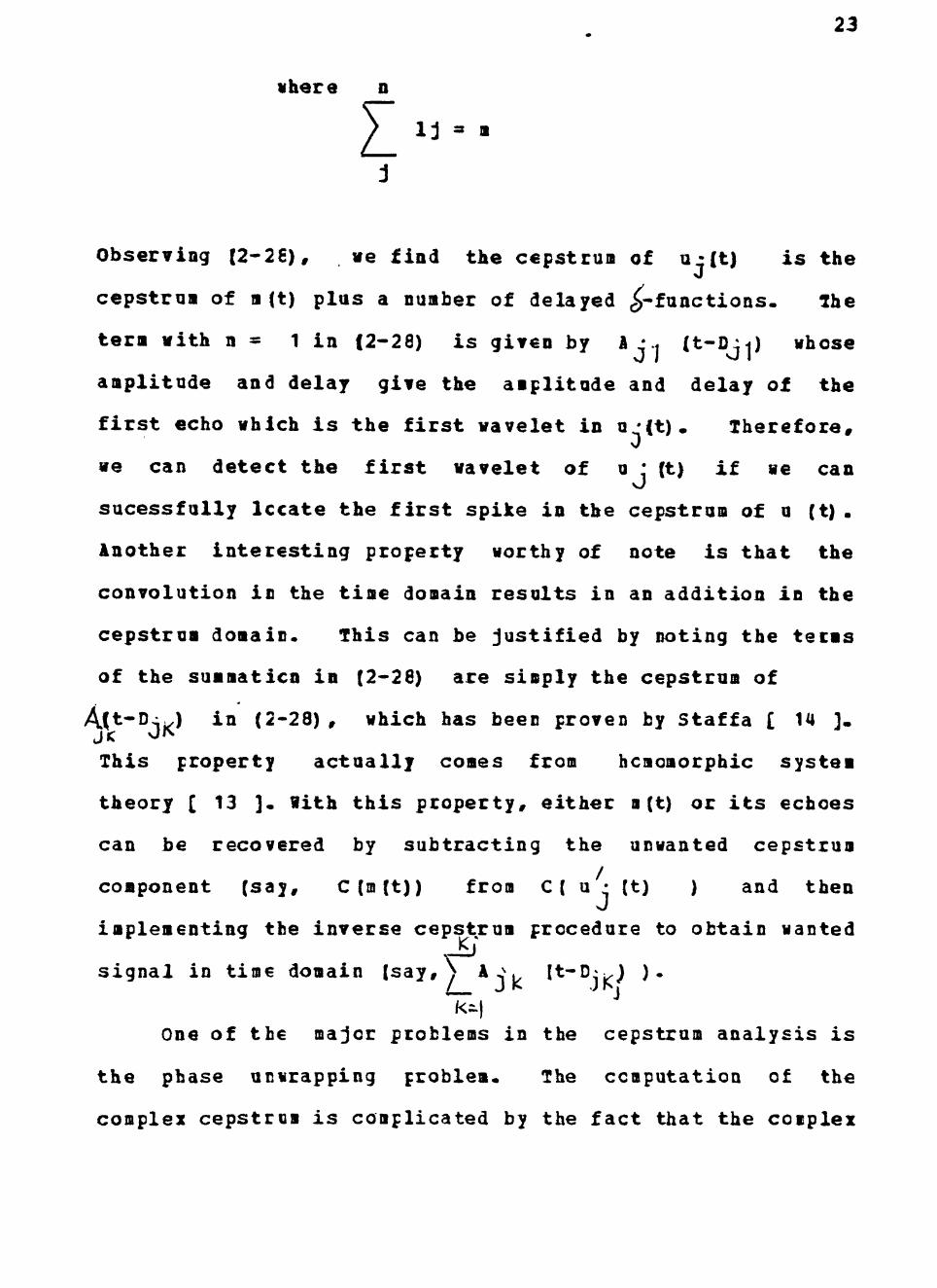
iihere D
~ lj = laquo
Observing (2-26) ve find the cepstrua of u-Jt) is the
cepstrum of m (t) plus a number of delayed ^-functions^ The
term with n 1 in (2-28) is given by A bull j (t-Dji) whose
amplitude and delay give the amplitude and delay of the
first echo which is the first wavelet in u(t) Therefore
we can detect the first wavelet of u bull (t) if we can
sucessfully Iccate the first spike in the cepstrum of u (t)
Another interesting property worthy of note is that the
convolution in the time domain results in an addition in the
cepstrum domain This can be justified by noting the teems
of the summaticn in (2-26) are simply the cepstrum of
Aft-Di) in (2-28) which has been proven by Staffa pound 14 1
This property actually comes from hcmomorphic system
theory pound 13 ]bull With this property either B(t) or its echoes
can be recovered by subtracting the unwanted cepstrum
component (say C(m(t)) from C ( u bull (t) ) and then
implementing the inverse cepstrum procedure to obtain wanted
signal in time domain (say) A (t-D^^) )
One of the major problems in the cepstrum analysis is
the phase unwrapping problem^ The computation of the
complex cepstrom is complicated by the fact that the coiplex
24
logarithm is snltivaloed^ If the imaginary part is computed
modulo 2 then discontinuities appear in the phase curve
This is not allowed since In ( F ( x (t) ) ) in (2-25) is the
Fourier transform of C(x(t)) and thus must be analytic on
the unit circle of the Z-plane There are several phase
unwrapping procedures which have been discussed in some
detail eg Smoothing the phase curve by adding a
correction curve pound 15 ] integrating the phase derivative pound
16 ] an adaptive numerical integration procedure pound 17 ]
and a recursive procedure to remove the linear phase pound 16 j
To avoid phase unwrapping problem and retain the property of
the homomorphic system we modify the original cepstrum as
follows The modified cepstrum is defined as
dF(x(t))dco|
) (2-29)
F(x(t)) I
1 CB(X(t)) laquo F
since there is no complex logarithm operation in (2-29)raquo laquo
do not have to worry about the phase unwrapping problem
The property of the Hcmomorphic deconvolution can be
justified by looking at the derivation of the modified
cepstrnm as follows He consider again a signal given by
the composite state U(t)
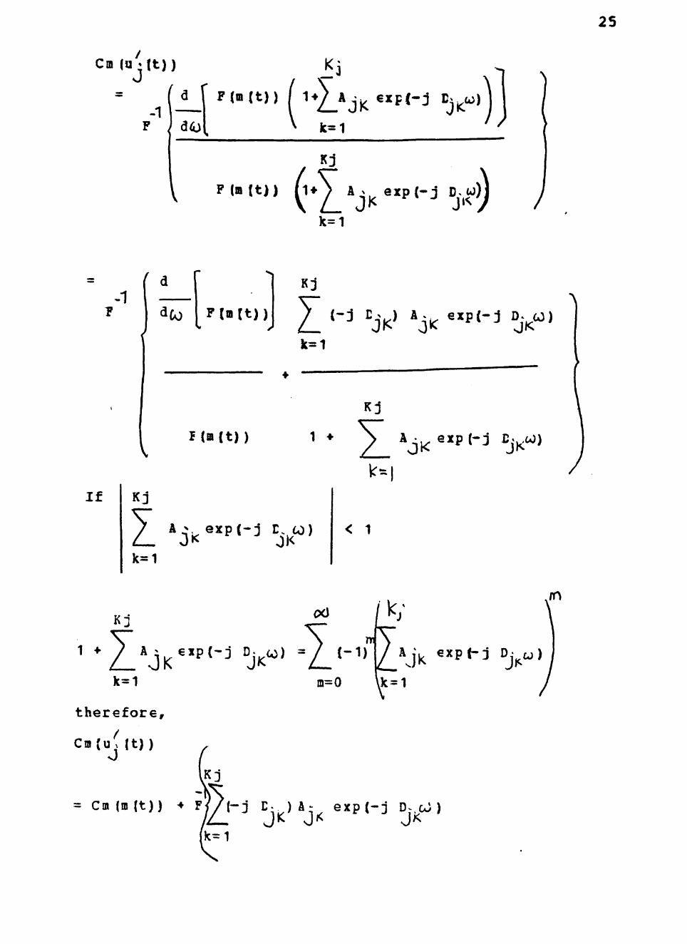
25
Cm (a ( t ) ) 0
lti d F ( m ( t ) )
-1 F dOl ^ k=1
Kj
( n i t ) ) h A A e x p ( - j Du)J
k=1
F 1 dco F ( m ( t ) )
Kj
Z JKgt 0lt ^^^ JK ^ k=1
V P ( a ( t ) ) 1 bull
Kj
I Ajj^ exp ( - j Ej^cJ)
I f Kj
I k=1
3k^P-^ iiK lt 1
Kj
1 gt
k=1 m=0 k=1
t h e r e f o r e
m
J D j u )
iKj
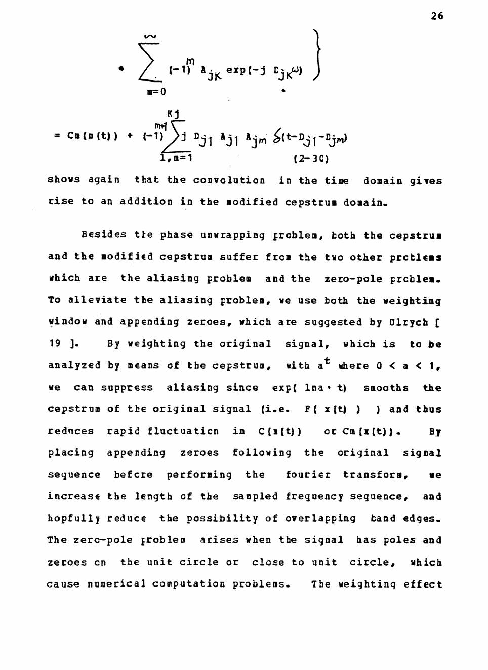
= Cm(m(t) ) + ^ 7 ^ ~ J ^ - J A w e x p ( - j DjcJ ) J lt Jlt Jgt^
k=1
26
bullgt
(-1)raquoj^expt-j Ej u
R3
l - D ^ D j ^ Aji Aj^ ^itl^^r^j^)
m=0
Kj
= Cm(m(t)) bull (-
r7m=1 (2-30)
shows again that the convolution in the time domain gives
rise to an addition in the modified cepstrum domain
Besides the phase unwrapping problem both the cepstrum
and the modified cepstrum suffer from the two other problems
which are the aliasing problem and the zero-pole problem
To alleviate tfce aliasing problem we use both the weighting
window and appending zeroes which are suggested by Olrych pound
19 ] By weighting the original signal which is to be
analyzed by means of the cepstrua nith a jhere 0 lt a lt 1
we can suppress aliasing since exp( Ina laquo t) smooths the
cepstrum of the original signal (ie F ( x (t) ) ) and thus
rednces rapid fluctuation in Cx(t)) orCm(x(t)) By
placing appending zeroes following the original signal
sequence before performing the fourier transform we
increase the length of the sampled frequency seguence and
hopfully reduce the possibility of overlapping band edges
The zero-pole problem arises when the signal has poles and
zeroes on the unit circle or close to unit circle which
cause numerical computation problems^ Tbe weighting effect
27
helps to alleviate this problem since weighting the signal
with a^ has effectively moved poles and zeroes further
inward away from the unit circle or equivalently it loves
the unit circle to a circle with larger radius exp (-Ina)
(Note that 0 lt a lt 1 and Ina lt 0 ) The weighting effect
does not promise the absolute solution to this problem
since if the signal is maximum phase or mixed phase with
poles and zeroes outside the unit circle poles and zeroes
are possibly scved to the unit circle by weighting Anyway
in most of the practical cases we can reduce the
aforementioned problems substantially by sufficiently
weighting the original time sequence In order to guarantee
an unaliased cepstrum we may initially weight the original
time sequence heavily and then try less weighting until
aliasing becomes a problem The least weighting where
aliasing does not cause a problem would be the weighting
chosen to iaplement cepstrum analysis in our case The
exponential weighting introduced above is also called
exponential windowing which really helps us to improve both
the aliasing problem and the problems associated with poles
and zeroes on the unit circle This fact has been justified
by Stoffa pound 1^ ] Before concluding this section we would
like to point out another problem which occnrs when we
generate a cottfosite state uj (t) (2-26) Me must multiply
m(t) by a scale factor K to ensure Aj|K lt 1 which iaplies
28
1 Kj
I k=1
jk bulllt^-degoltgt lt 1
and hence we have no divergence problem Alternat ive ly we
may use exponential weighting again which makes the
re f l ec tor s e r i e s minimum phase i f we weight u^ (t) O
sufficiently In our case we use both the scale factor and
weighting to ecsure convergence To conclude this section
we summarize loth advantages and limitations of the cepstrum
technique Ibe major advantages are its detectability and
bullblind deconvolution property The blind means that it
can perform deconvolution without knowing the input ie can
find the input from the cepstrum if the cepstrum of the
input does not mix significantly with those of the delayed
echoes The primary disadvantage of the cepstrum analysis
is its sensitivity tc noise and we have selected ML
estimation to estimate states before using the cepstrum
Three algoritlms to perform BL estimation and cepstrum
detection are to be presented in the next section
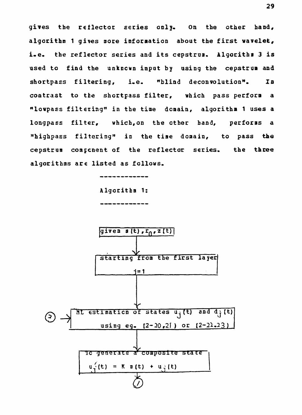
Algorithfs
Algorithi 1 performs MI estixation and cepstrum detecshy
tion with both the input and output given Algorithm 2 pershy
forms HL estimation and ordinary deconvolution for
comparision It has a simpler aathematical approach and
29
gives the reilectoc series only On the other hand
algorithm 1 gives more information about the first wavelet
ie the reflector series and its cepstrua Algorithi 3 is
used to find the unknown input by using the cepstrum and
shortpass filtering ie blind deconvolution In
contrast to the shortpass filter which pass perform a
lowpass filtering in the time domain algorithm 1 uses a
longpass filter whichon the other hand performs a
highpass filtering in the time domain to pass the
cepstrum component of the reflector series the three
algorithms are listed as follows
Algorithm 1
[given a (t) r^z (t)]
plusmn starting from tbe first layer
X x-N pML es t imat ion of s t a t e s u gt (t) and dj (t)
using e g (2-Q2n or (2-2133)
uUt) = K ffl(t) bull U l t ) aJ ^
^
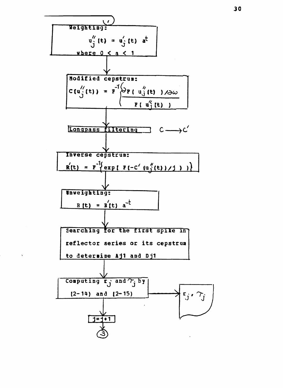
weighting
laquot (t) u (t) a
where Q lt a lt 1
Nlt Hodified cepstrum
CCUj(t)) = F (5gtF( u^lt) ) aco
g ( qj (t) )
gt ^
llonqpass f i l ter ing bullgtc
d inverse cepstrum
R(t) ^ F^jexp( F(-C^ (uj(t))j ) ))
Vnweighting
B (t) - B (t) a ^
for Searching for the first spike in~
reflector series or its cepstrum
to determine Ajl and Dji
^ Computing r ^ and O- by
(2-14) and (2-15)
Jiil
bull J J
j^j1
30
31
YES gt
f STOP J
Algorithm 2
given a(t)r^z(t)
^ r starting irom the first layer
bull laquo plusmn HL estimation of states U(t) and d (t)
sJ o
gtr Taking the Fourier tranform of u (t)
and m (t) to obtain
llj(60) and H (cj)
N^ suDtraction
B (g)) == Oj (cj) -EM
N Inverse Fourier transform
-1 B(t) ^ F ( R tu)) )| ^
D same
as algorithm 1
Algorithm 3
32
given r^ yTflT
^ l Weighting
ztt) = z( t ) a
N ^ Modiried cepstrum
Cm(z(t))
V Shortpass riitermg
to pass the cepstrum before the
first spike ^
^r Inverse cepstrum
to obtain m (t)
N^ Bnweignting
m(t) = m (t) a -t
33
Simulation ^nd results
In this section we shall present a simulation model
for a 7-layer earth system and implement the algorithms menshy
tioned in the previous section The simulation model is
shown in fig4^ Bsing the VAX 11780 as a programming tool
and also using COHTAL image processing system as a graphic
aid we can esily iaplement the algorithms and estimate r -J
and ^ bull
CI) XS generate a s y t h e t i c seismogram
Be f i r s t generate an impulse response for the 1- layer
system using a r a y - t r a c i n g technique as d iscussed in the
f i r s t s e c t i o n cf t h i s chapter Takinq t h i s qenerated imshy
pulse response as t h a t from the bottom layer of the 7 - l a y e r
sys tem we employ Bobinson^s formula (2-11) t o obtain the
impulse response of a 2 - layer system Continuing i n t h i s
way we can f i n a l l y generate an impulse response for the
7 - l a y e r s y s t e m To obtain a s y n t h e t i c seismogram for the
7 - l a y e r s y s t e a we have to convolve the input s ignature with
i t s impulse response The noisy s y n t h e t i c seismogram i s obshy
t a i n e d by adding a Gaussian white noise to the above se i smoshy
gram The Gaossian white no i se i s generated by a FOBTBAN
program NOISEIOH which i s l i s t e d in the appendix^ The input
s i g n a t u r e m(t) used t o generate the seismogram i s
m(t )-1360t e x p ( - 5 0 0 t ) 0 5 e x p ( - 1 5 3 t ) s i n ( 2 t 0 0 6 )
5 At
6 At
QCit
7 At
5 At
10 At
TQ=01
bull r j=04
plusmn^ r2=-02
r3=05
r^=03
VO-2
rg=09
r^=08
Figure 4 The s imulated 7 - l a y e r earth system
34
35
The sampling time of m (t) is 15 msec The generated m (t) is
shown in fig1euro
(2) laplementation of a^rqorithms
Be use algorithm 1 and 2 to estimate rs and^^s from
the impulse response and synthetic seismogram assuming the
input of the system is given Both algorithm 1 and algorshy
ithm 2 perform BL estimation and deconvolution (algorithi 1
performs Bomomorphic deconvolution and algorithm 1 performs
ordinary deconvolution) Algorithm 2 has a simpler matheshy
matical approach and gives only the reflector series used to
estimate rC andOraquo This gives a limitation of algorithm 2
since it may fail to detect the first spike in the reflector
series if noise is so serious as to obscure the location of
the first spike On the other hand the algorithm 1 gives
both the reflector series and its cepstrum If detection of
the first spike can not be obtained in the reflector secies
we may find the first spike from its cepstrum Osually the
cepstrum is less noisy than the reflector series since noise
in the reflector series has been enhanced by unweighting
Also note that the reflector series of algorithm 2 is recovshy
ered from u(t) = K m (t) bull J ^ instead of ^j Ct) bull Thereshy
fore laquoe have to neglect the spike appearing at the zero
point which is caused by Km(t) The first spike after the
zero point is the real first spike we expect The estimashy
tion error is computed by
36
(estimated value) - (actual value)
error - mdash - mdash mdash _ _ _
(actual value)
Strictly speaking estimation error contains not only the
estimation error from the estimation scheme but also the
computation error of the digital computer In our case we
use the term estimation error to include these two errors
In addition the estimation error of the one-way travel time
is almost zero if we can detect the first spike which is
the cepstrum of the first wavelet in ui(t) from either the O
reflector series or its cepstrum Therefore we shall comshy
pute only the estimation error of the reflection coefficient
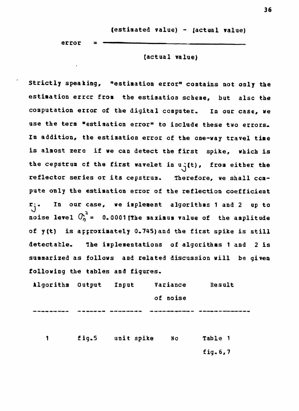
r^ In our case we implement algorithms 1 and 2 up to
noise level 0)^ raquo 00001 (The maximum value of the amplitude
of y(t) is approximately 0745)and the first spike is still
detectable The iaplementations of algorithms 1 and 2 is
summarized as follows and related discussion will be given
following the tables and figures
Algorithm Output Input Variance Result
of noise
fig5 unit spike No Table 1
fig67
37
1 f i g 8 same 0 000001 Table 2
f i g 9 10
1 f i g 1 1 same 0 00001 Table 3
f i g 1 2 1 3
1 f i g 1 4 same 00CO1 Table 4
f i g 15 16
1 f i g 17 f i g 18 Mo Table 5
f i g 1 9 2 0
1 f i g 2 1 f i g 1 8 0 000001 Table 6
f i g 2 2 2 3
1 fig24 fig^lB 000001 Table 7
fig2526
1 f i g 2 7 f i g 18 00001 Table 8
f i g 2 8 2 9
2 f i g 1 7 f i g 18 No Table 9
f i g 30
2 f i g 2 1 f i g 1 8 0C00O01 Table 10
f i g 3 1
38
2 f i g 2 4 f i g 1 8 000001 Table 11
f i g 32
2 f i g 2 7 f i g 18 00001 Table 12
fig^33
39
TABLE 1
Estimates of r and T using algorithm 1 ((^= 0 )
03999695
-01999689
04998601
02998001
01998157
08990071
07917798
j (sec)
50
40
60
80
70
50
100
layer
1
2
3
4
5
6
7
error of r
-000007625
-000015550
-000027980
-000066633
-000092150
-000110322
-001027525
40
TABLE 2
E s t i m a t e s cf r a n d ^ j u s i n g a l g o r i t h m 1 (0^ =0 000001)
03990620
-01992678
04975078
02979723
01973471
08927326
07202561
J (sec)
50
40
60
80
70
50
100
layer
1
2
3
4
5
6
7
error of r
-00023450
-00036610
-00049844
-00067590
-00132645
-00080748
-00996799
41
Figure 5 The impulse response of the 7-layer system Ifig-4)
igure 6 The reflector series of the layer 7 with no noise corruption
42
Figure 7 The ceps t rum of f i g 6 with weighting a=096
i q u r e 8 The no i sy impulse r e sponse with noise 0)gt =0 000C01 Fig
43
Figure 9 The r e f l e c t o r s e r i e s of the l aye r 7 with noise =0000001
Figure 10 The cepstrum of f i g 9 with weighting a = C96
44
TABLE 3
E s t i m a t e s cf r j and O j us ing a l g o r i t h m 1 ( =0 00001)
03970979
-01977552
04924526
02940953
01921248
08795565
06001474
j (sec)
50
40
60
80
70
50
100
layer
1
2
3
4
5
6
7
error of r
-00050525
-00112240
-00150000
-00196823
-00393760
-00227150
-02498229
45
TABLE 4
E s t i m a t e s of r j a n d ^ us ing a l g o r i t h m 1 (0^^ = 0 0001)
03908762
-01930114
04767275
02824915
01764654
08411036
03804527
^ (sec) J
50
40
60
80
70
50
100
layer
1
2
3
4
5
6
7
error of r w
-00228095
-00349430
-00465450
-00583617
-01176730
-00654404
-05244341
46
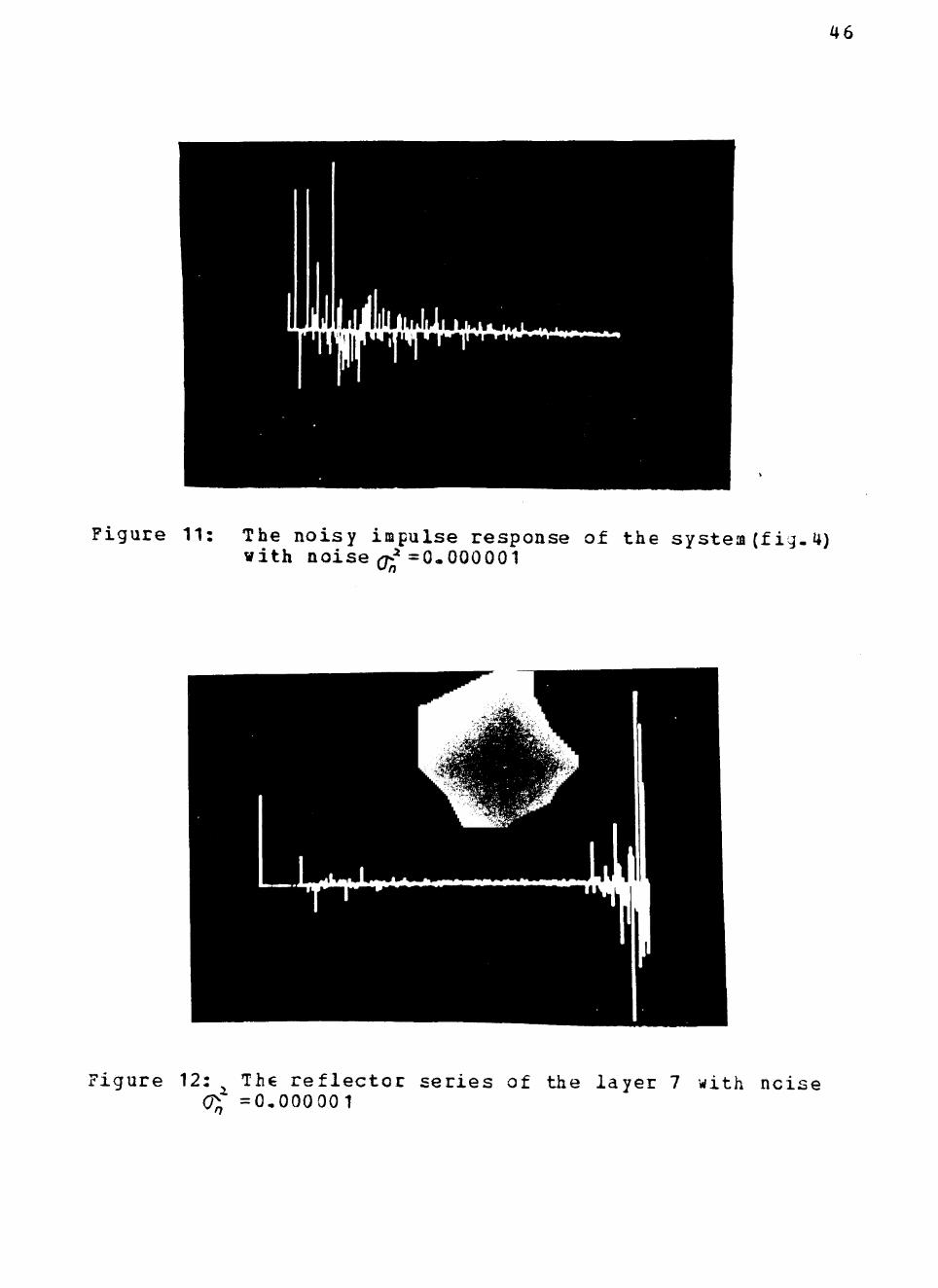
Figure 11 The noisy impulse response of the system (fig-4) with noise (Tn
i _ =0000001
Figure 12 The reflector series of the layer 7 with noise 0) =0000001
47
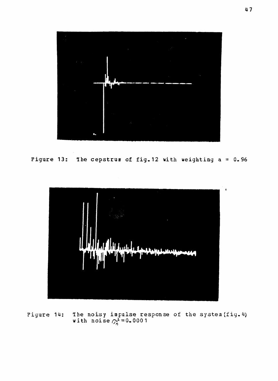
Figure 13 Ihe ceps t ruu of f ig 12 with weighting a = 096
Figure 14 The noisy impulse response of the system ( f i g 4) with noise7v^ = 0000 1
48
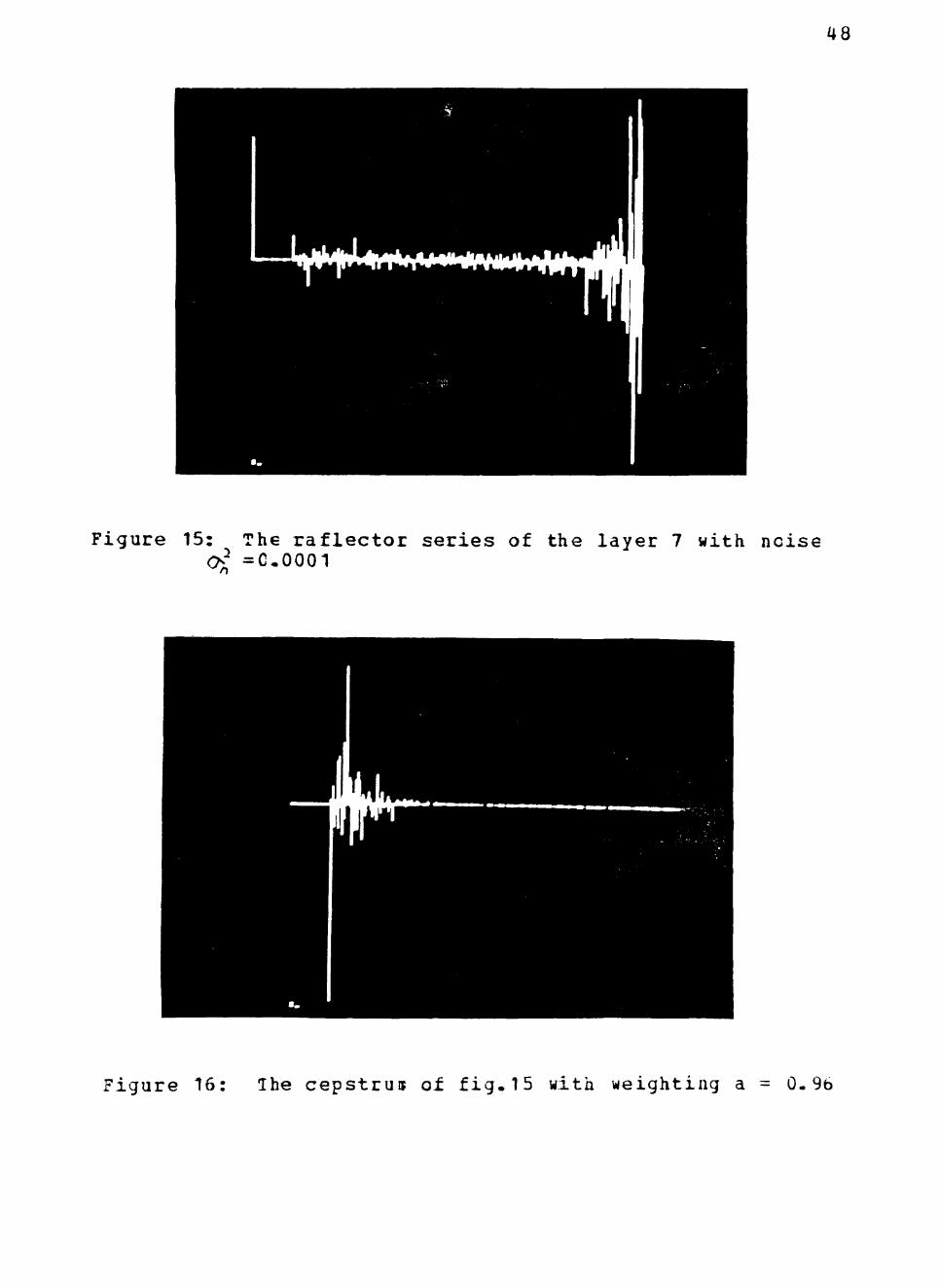
Figure 15 The raflector series of the layer 7 with noise ltgt =0 0001
n
Figure 16 The c e p s t r u i of f i g 15 with weighting a = 096
49
TABLE 5
Est imates of zt and O- from seismogram using algorithm 1 ( ^ ^ =0)
3 ^ (sec)
vi
03999693 0074999996
-01999689 0059999999
04998601 0090000004
02998001 0120000000
01998158 0105000000
08990070 0074999973
07917758 0150000000
layer
1
2
3
4
5
6
7
error of r
-000007675
-000015550
-000027980
-000066633
-000092100
-000110333
-001028025
50
TABLE 6
Estimates of r andO- from seismogram using algorith 0 vJ^i=0000001)
i 1 (
03836054
-02080411
05103642
03151133
02053305
09163057
08715951
0-(sec)
067499996
005999999
090000004
012000000
010500000
007499997
015000000
layer
1
2
3
4
5
6
7
error of r
-00409865
+00402055
+00207284
+00503776
+002665250
00181174
+0089493875
51
Figure 17 The reflection seismogram of fig4 with corruption
no noise
Figure 18 The input signature to the system fig4 to generate the seismogran
52
Figure 19 The r e f l e c t o r s e r i e s of the layer 7 with no noise corruption
Figure 20 Ihe cepstrun of f i g 1 9 with weighting a = 0S6
53
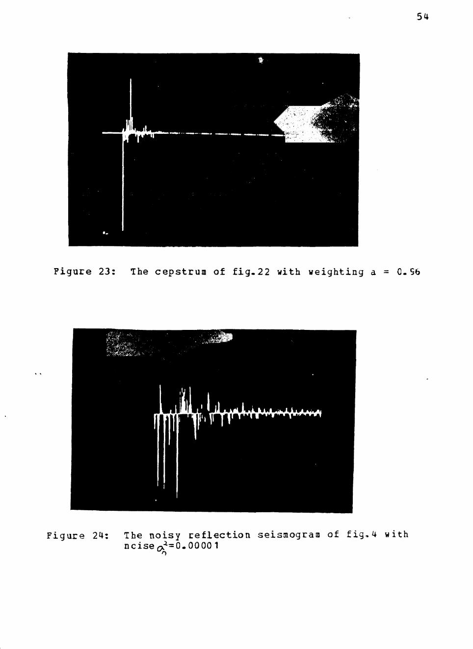
Figure 21 The noisy reflection seismogram of fig4 with noise 0^=0000001
Figure 22 The reflector series of the layer 7 with ncise 0- =0000001
54
Figure 23 The cepstrum of f ig 22 with weighting a = CS6
Figure 24 The noisy nciser^= 000 00 1
n
reflection seismogram of fig4 with
55
TABLE 7
E s t i m a t e s of r and ^ from seismogram u s i n g a l g o r i t h a i 1 ( gtgtfraquo=G00001) Oo
3
03850933
-02097894
05164353
03143446
02099267
09359658
13083239
O^(sec)
0075000003
0060000001
0090000005
0120000000
0104999999
0075000003
0150000000
layer
1 CVJ
3
4
5
6
7
error of r
-003726675
+004894700
+003287060
+004781533
+004963350
+003996200
0635404875
l
56
TABLE 8
Estimates of r bull and from seismogram using algorithm 1 Q- =00001)
0
y^
3
03897932
-02153131
05360212
03116841
02270585
10040127
-14135658
^j(sec)
074999996
005999999
009000004
012000000
010500000
007499973
015000001
layer
1 CVJ
3
4
5
6
7
error of r
-002551712
007656551
007204240
003894712
013529250
011556966
too large
57
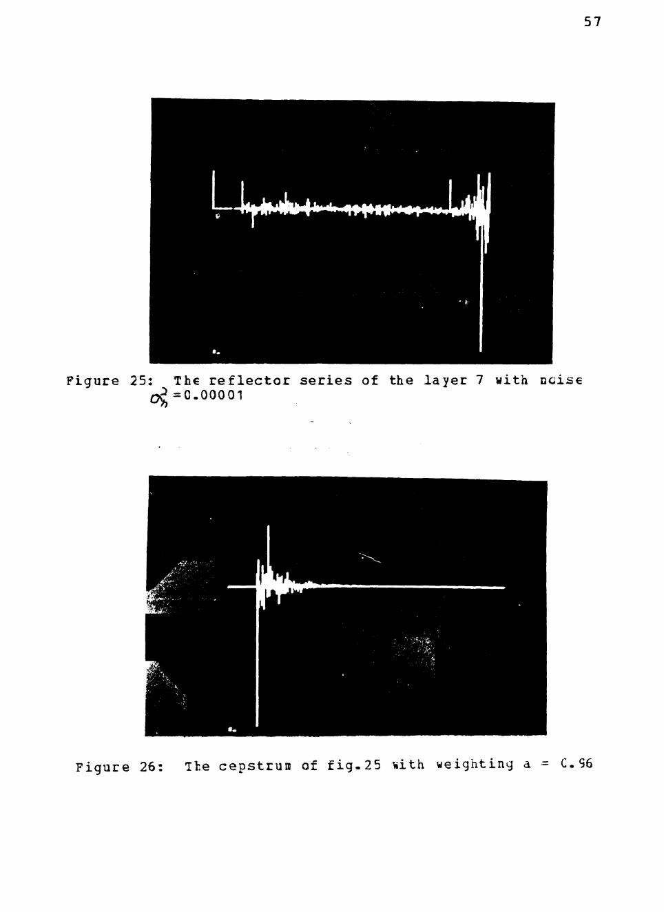
Figure 25 The r e f l e c t o r s e r i e s of the l aye r 7 with noise ^ = 0 0 0 0 0 1
Figure 26 The ceps t run of f i g 2 5 with weighting a = C S6
58
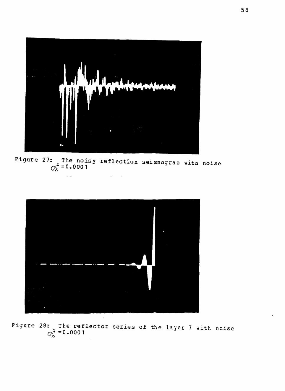
Figure 27 The noisy reflection seismogram witn
lt ^ 00001 noise
Figure 28 The reflector 0 =C0001
series of the layer 7 with noise
59
Figure 29 The cepstrum of f i g 28 with weighting a = C S6
Figure 30 The r e f l e c t o r s e r i e s of the layer 7 with nc no i se corruption
60
TABLE 9
Est imates of r- and O from seismogram using algorithm 2(c^ = J gt 0)
3
03999693
-01999689
04998601
02998601
01998158
08990070
07917758
atsec)
0074999996
0059999999
0090000004
0120000000
0105000000
0074999973
0150000000
layer
1
2
3
4
5
6
7
y^ error of r
-000007675
-000015550
-000027981
-000066633
-000092100
-001028025
-001028025
61
TABLE 10
Estimates of r and^raquo from seismogra ^ J =0000001)
using algorithm 2(G
3
04006643
-02008083
05027021
02996138
02018067
09075617
08867384
r C s e c )
0074999996
0059999999
0090000004
0120000000
0105000000
0074999973
0150000000
layer
1 CVJ
3
4
5
6
7
error of r xJ
+000166075
+000404150
+000540420
-000128733
+000903351
0009033500
0108423000
62
Figure 31 The reflector series of the layer 7 with noise Qlt^ =C000001
Figure 32 The reflector series of the layer 7 with noise ^^=000001
63
TABLE 11
Estimates of r andOfrom seismogram using algorithm 2 0^ ^ J =0 00001)
3
04021672
-02026290
05088857
02992276
02062335
09265897
11768117
O^(sec)
0074999996
0059999999
0090000004
0120000000
0105000000
0074999973
0150000000
layer
1
CVJ
3
4
5
6
7
error of r
0005418
0013145
00177714
-00025747
00311675
00295441
0471014625
64
TABLE 12
Estimates of r and^from seismogram using algorithm 2 J J =00001)
04069195
-02084359
05287915
02981632
02214152
09920729
127666025
^j(sec)
0074999996
0059999999
0090000004
0120000000
0105000000
0074999973
0150000000
layer
1
CVJ
3
4
5
6
7
error of r vJ
001729875
004217950
005758300
-0006122606
0107076000
0102303222
too large
65
Figure 33 The reflector series of the layer 7 with noise
^n 2 =00001
66
the following conclusions may be drawn from the results of
the simulation (i) Estimation is more accurate at upper
layers and becomes inaccurate as we proceed to the deeper
layers This is because the deeper layers have less
information than that of the upper layers (Hecall that a(t)
reflects only information within and below the layer j) In
Table 7 which shows the result of the fost serious noise
level OS = 0CC01 we still have pretty good estimates for
the upper 5 layers (ii)Estimation is more accurate for the
layers with higher reflection coefficients for instance
the estimate cf r^ for layer 6 in each table (the actual
value of r^ = C9) (iii) The large amplitudes appearing at
the end of the reflector series in the figures are due to
noise which has been enhanced by unweighting^ This gives a
disadvantage in using the exponential window
If the input of the system is not given we may use
algorithm 3 tc find the input but algorithm 3 is successful
in finding the unit spike input from the impulse response
and fails to find the inpnt other than the unit spike |as
shown in fig 16) from the synthetic seismogram This is
because the shortpass filter used in algorithm 3 passes only
the cepstrum component before the first spike and filters
oat that after the first spike which may contain part of
the informaticn of the input cepstrum This fact can be
seen bj looking at the cepstrua of the reflected seismogram
67
(the output to the 7-layer system in fig 4) as shown in
fig34 The results of implementing algorithm 3 are
sammari2ed as follows
Algorithm Impulse response Variance Input
3
3
3
3
fig5
fig8
fig11
fig14
of noise
No
0 000001
000001
00001
fig35
fig36
fig^37
fig^38
68
V
F i g u r e 34 The ceps t rum of t h e s y n t h e t i c seisiaogram of the system f i g 4
69
Ccmparision with Habiti-Ashrafi work
As menticned before Babibi-Ashrafi used a suboptiaal
scheme to detect the first wavelet in u It) [ 6 ]bull fie was
not able to obtain estimates for layers with smaller reflecshy
tion coefficient if noise appeared in the seismogram Osing
the cepstrum technique we can detect the first wavelet for
every layer if the first spike in the reflector series and
its cepstrum is detectable^ We have implemented our algorshy
ithms up to noise level - 0^0001 and the first spike is
still detectable although the aiplitude is inaccurate for
the deeper layers^ The disadvantage of our approach is that
cepstrom detection is cospletely determined by the detectashy
bility of the first spike In other words cepstrum detecshy
tion will fail if we can not see the first spike in the
reflector series or its cepstrum
70
Figure 35 The input recovered from the cepstrum with no noise corruption
Figure 36 The input recovered from the cepstrum corrui^ted by noise Q- =0000001
71
Figure 37 The input recovered from the cepstrum corrupted by noise i7r-=C 00001 ltgt
Figure 38 The input by noise
recovered from the cepstrua corrupted 2 =00001 o^
CHAPTER III
CCNTIHOOaS SEISaiC IHVSfiSS PBOBISH
Introduction
This chapter presents an analytic solution to the inshy
verse problem for the earth system with continuous impemdash
dance^ The method used is the so-called one-dimensional inshy
verse scattering problem The idea originates from the
scattering problem of quantum mechanics where the scattershy
ing pattern can be predicted and discribed by a special
eguation well known as the Schroedinger eguation Newton [
20 ] has derived necessary details for the scattering theoshy
ry Here we are interested in an inverse scattering problem
similar to the one we saw in the last chapter Assuming the
impulse response from the continuous earth system (ie^ the
earth system with continuous impedance) is given we shall
try to identify the continuous earth system or eguivalent-
ly to find the impedance as a function of the travel time
The analytic solution is approached by first transforming
the elastic wave eguation into a one-dimensional Schroediger
eguation and then using the results already available on
the inverse scattering problem to recover the potential of
72
73
the Schroedinger eguation from the impulse response cf the
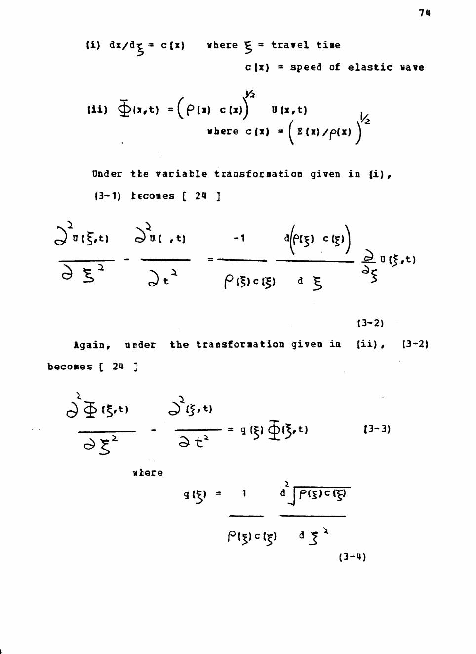
continuous earth system^ Recovering the potential involves
solving the so-called Gelfand-Levitan integral equation^ We
shall try different numerical methods to solve this integral
equation^ Once the potential is recovered we can cttain
the impedance from the potentials
transformation
The medium to be probed with a plane wave at normal inshy
cidence is assumed to be an isotropic and homogeneous medium
whose elastic parameters vary continuously as a function of
the space coordinate Xm The elastic wave eguation for small
displacement is given by
p(x)
^ tJ(xt)
gt t
^x
^W
^ 0|xt)
C^X
13-1)
where Pw = the mass density of the earth system^
0 (xt) = the displacement of vibration
E fx) =Ax) bull 2 ^ (X) for compressional wave
^ (X) for transversal wave
-X rW = tame parameters
let
74
(i) dxdr = c(x) where = travel time
c Ix) = speed of elastic wave
Iii) ^(xt) =(^PU) c(j)J Olxt)
bull here cji) =fE(i)p(x) j k
Dnder t i e variable transformation given in ( i )
(3-1) teurocomes [ 2n ]
o ) Utl^rt) ^ t J ( t ) - 1 dpC ) c ( | )
^ 1 gt ^t^ Pi|)ci5) d mdash ^a(|t)
(3-2)
Again under the transformation given in (ii) 13-2)
becomes [ 24 j
mdash = gn$l^t) (3-3)
^S Sf
wtere
gc^) JpiiKlf)
Pipcip aj^ (3 -4)
75
whose Fourier transform is
(Jlt^i^jLC) = g (5)^(5^0) (3-5)
Equation (3-5) is recognized as a one-dimensional
Schroedinger equation In this case the impedance c aust
be at least continous otherwise the transformation (ii) and
the potential q in (3-4) are not well-defined By (3-4) we
see that q^) vanishes whenever the elastic medius is
homogeneous or whenever c is a linear function of the
travel time
Continuous inverse-scattering problem
The solution of the inverse scattering problem for the
one-dimensional Schroedinger equation has been discussed in
detail by Faddeev [ 21 ] Hoses and deRidder [ 22 ] and
Kay [ 23 ]bull Ihey applied the techniques used to solve the
inverse-scattering problem for the radial Schroedinger eguashy
tion to solve the inverse scattering problem for the one-dishy
mensional Schroedinger eguation^ The medium illustrated in
fig39 is now considered for the continuous inverse scattershy
ing problem Following the work done by Hare and Aki [ 24
] we define the travel time as follows
5 ) = vlt for X lt 0
76
(3-6)
(3-7)
In fig 39 Sij are the elements of the so-called scattering
matrix where
S ((O) - Fourier transform of the reflected impulse
response of medium for x gt 0
S -Cw) = Fourier transform of the transmitted
impulse response of medium for x gt^ Q
If the probing wave goes from the other side the above
responses are referred tc as S (pound0) and S (o) Therefore
the scattering matrix is simply
^S JO)
Siu) = 11
S iu)
^r (3-8)
The medium in fig39 is probed with plane waves at normal
incidence for all frequencies This is equivalent to
probing the medium with a normally icident impulsive wave
Incident planei^ave
Homogeneous half-space
Po^o
(^QCQ^expl-jtoxCQ) I
I Ref 1 ected 4 - v A 4 W ^ plane wave
^ I pQZQ)S^^Lo)exp3^gt^c^)
1
Heterogeneous med i urn
P(x) c(x)
Homogeneous half-space
^n+l ^n+1
fpansmittei i t ted plane
wave
( n+lS+l Si iMexp(o7-)
exp(j (x-b) )
S+1
x=0 x=a x=b
F i g u r e 39 The medium used for i l l u s t r a t i o n of i n v e r s e s c a t t e r i n g problem
78
The boundary location fcetween the homogeneous half-space
( Pc ) and the heterogeneous medium (P(x) c (x)) is chosen at
x = a instead of x = 0 for greater generality since the
recorder is not generally located right on the surface Two
impulse responses measured at different locations in the
homogeneous half-space differ only by a time shift The
so-called inverse-scattering problem is to recover the poshy
tential q(5) from the observed scattering data Knowing
q(^) we can recover the impedance of the earth system
This procedure can be illustrated as follows
Suppose S (CO) is obtained by a scattering experiment
then we can find the impulse response R(t) by taking the inshy
verse Fourier transform of S (co) i e
R(t) = 1 f^ -jlaquoigtt
pound ((J) bull e dt (3-9)
Next we use Gaifand-Levitan i n t e g r a l equation (3-72) to f ind
the kernel K ( | t ) which i s re la ted to the p o t e n t i a l q ( | ) by
g (5) = 2 d K ( | 5 ) d ^ (3-10)
The Gelfand-Levitan integral equation discussed in refershy
ence [ 21 ] is given by
K(5t) = -R(|+t) - 1 K(5t) a(Ht) dT (3-11)
79
In pract i ce the lower integral l i n i t - 0 0 in (3-11) can be
replaced by - t s ince the impulse response RJt) i s one-sided^
(3-11) can be uritten as
r Kift) = -mftt) -
-t K(5gt) Bf^+t) dT- (3-12)
Op to this stage we can summarize the algorithm to
implement the inverse scattering problem as follows^
(1) S^Jicd) is given
(2) find R (t) by (3-9)
(3) Evaluate K(|t) by (3-12) |A-1)
(4) B e c o v e r q J ^ by (3-10)
(5) Eecover the iipedance Z(P) by (3-4)
Examining (5) in the algorithm (A-1) we have to solve (3-4)
which is a second order differential eguation and can be
rewritten as fellows^
5S 3 q() Zt) = 0 (3-13)
Vl Khere Z f^) = lft|)c[|) )
80
Instead of solving (3-13) directly A second method is
suggested by Eerryman and Greene pound 26 ] Noting that (3-13)
is identical tc the one-dinensional Schroediger equation as
0 gt 0 we shall use this similarity to obtain an algorithm
recovering Z (sect) without actually solving (3-13)^ Faddeev
[21 ) has shown that the Jost solutions for the
one-dimensional Schroedinger equation have the form
J^ iS^) = ex P il^p for ltlt 0
r exp(ju)sect) bull
y^
K(5raquo exp(jio7) d7-
5 for5gt 0
(3-14)
where K ^T) is the kernel shown in (3-12) bull
Using the fact that (3-13) is equivalent to (3-5) ^sCo^^O^
and the Jost solutions given above we find
2(f ) = C J^(50)
(3 -15)
where C i s a cer ta in constant to be determined
81
To determine C we consider
P = C
1=0
Therefore (3-15) becomes
2 ( | ) = Z (0)
(3-16)
Using ( 3 - 1 6 ) we can recover Zjf) knowing only K |g gt - )
without bothering t o compute q (5) in (3-10) and recover Z (^)
in ( 3 - 4 ) The algorithm (A-1) can be modified as f o l l o w s
(1) S (Co) i s g iven
(2) Find R (t) by (3-9)
(3) Evaluate K (^t) by (3-12)
(4) Recover Z (P) by (3-16)
(A-2)
We s h a l l use tfce algorithm IA-2) instead of (A-1) to so lve
the inverse s c a t t e r i n g problem numerically in the next
s e c t i o n -
82
Humerical s o l u t i o n and s imulat ion r e s u l t s
The major part i n s o l v i n g inverse s c a t t e r i n g problem
l i e s in s o l v i n g the Gelfand-Levintan i n t e g r a l equation- We
s h a l l use three numerical i n t e g r a t i o n r u l e s to approximate
the i n t e g r a l equat ion They are the trapezo id r u l e Simpshy
s o n s 13 r u l e and Simpsons 3 8 r u l e The numerical i n t e shy
grat ion using the trapezo id rule i s a two-point i n t e g r a t i o n
This i s t o s a y i f f (x) i s sampled a t xO x 1 x2 xn
with sampling i n t e r v a l h then
x l
fx) dx = f(xO) bull f (x1) ) h 2
xO
To approximate the i n t e g r a t i o n of f (x) from xO to x1 we
need only two sampled f ( x ) s at xO and x 1 The advantage of
using the trapezoid ru le i s that there i s no r e s t r i c t i o n on
the sampling r a t e i e n The disadvantage i s i t s larger 3 (2)
truncat ion error ( h f 12 ) compared with the other two
To improve the truncat ion e r r o r we may use Simpsons 13 ^ laquo bull gt ru le and Simpsons 3 8 ru le whose truncat ion errors are h fA
i- (4) (0 ^
and 3 h f 8 0 r e s p e c t i v e l y where f denotes i - t h d e r i shy
v a t i v e of f The disadvantages of using the aformentioned
approximation ru le s are the l i m i t a t i o n on the sampling ra te
The Simpsons 13 ru le i s a t h r e e - p o i n t i n t e g r a t i o n approxishy
mation and requires n be an odd number The Simpsons 38
rule i s a four -po in t i n t e g r a t i o n and requ ire s n to be of the
form 4 + 3m where m i s an i n t e g e r inc luding zero
83
He shall use the above three numerical integration
rules to approximate the Gelfand-Ievitan integral equation
(3-12) By discretizing (3-12) and letting mdash ^ nh
t mdash ^ h we can find the following matrix formulation using
the trapezoid rule
I bull h
I
o
6l Hi
1 ^2 3 bull
1
a-j R^ Ro
^
V2gti-l
^-f in
hk (n-n1)
hk n-n+2)
hk (n-n^3)
hk tnn-1)
1 bull hk(nn)
0
0
0
0
1 J
where k(n8) = K(nm) (3-17)
1 - hK(nn)2
Note that we have used knm) instead of K(nm) to obtain
(3-17) Therefore laquoeuro need to perform a variable change to
obtain K(nm) from k|nm) whenever k[nm) is available
Eguation (3-17) has an advantageous form for aatrix
inversion since Householders formula can be exploited to
reduce computation especially Hhea the dimension cf the
matrix is large Equation (3-17) can be rewritten as
0
0
0
hR
1
0
C
1 bull
bull bull 0 hR 1
hR1 hfi
hBi
hR^
hR-4 bB
hR^ hR
hR l+hj hR-
hR hR hR^^1 + ^2T|
KJc(n-n+r)
hk n-n2)
hk in-n3)
hk (n-n1)
1+hk (nn)
0
0
^
I
To obtain k(nif) we start from n=1 ie^ the 2 by 2 square
matrix^ Due to the symmetric property of the square matrix
we first invert the 2 by 2 square matrix and take its
inverse as the central block to invert the 4 by 4 square
matrix at the next stage After inverting the 4 by 4
matrix we again take this 4 by 4 inverted matrix as the
central block to invert the 6 by 6 matrix next Continuing
in this way ve can eventually invert the 2n by 2n matrix
By doing this we save a lot of work in inverting a 2n by 2n
matrix since we need simply to take care of two 2n by 1
column matrices and two 1 by 2n row matrices to obtain the
inverse of a 2n by 2n satrix when the 2n-2 by 2n-2 central
block is already ^ inverted Me shall illustrate this
procedure by inverting a 6 by 6 matrix of the form (3-17)
which is given by
85
A = 1
0
0
deg 0
hB-
0
1 1 0
hR-j
hR^
C
0
1
hR-|
hR^
hR3
0
0
hR^
UhR^
hR3
hB^
0 bfl^ 1
hR-1 1 hR^ 1
hR2 h B j
ha^ 1 hB4
1hH^ hS^
hR^ 11
13-18)
(3-18) can he decomposed i n t o
A = 1 0 0 0 0 0
0 c e n t r a l
I 0
0
hR
hP
^
hR^
A T
0
0
b l o c k
C 0 0 0 1
a C 0 0 0
0 l(bH-| hfi^ hR^ hR^ hfl^ hRlt5 )
0
0
K ^
)
c
(3 -19)
86
On examining (3 -19) i t i s easy to use twice Householders
formula to i n v e r t the 6 by 6 matrix Equation (3-19) has the
form 1- T
A = B - c r r c (3-20) T T = (B bull c r) bull r e
Usinq Househclders formula we have
A = (B bull c r ) -1 SI S]
- (B bull c r) r^(1 bullbull c^(E +0 r) r^) c (B ^c r)
(3-21)
The rest of the problem in |3-21) is to find (B bull c r)^ To
achieve this ve aqain use Householders formula -1 -1 -7 -1 -1
B c r ) = B - B c ( 1 + r B c ) r B (3-22)
By not ing that -1
B c = c
and -1
r E c = r c laquo h^2
we can reduce (3-22) t o - 1 gt1 - 1
(pound + C r ) = B - c ( 1 hR^z) r B (3-23)
To perform r E we need only mult iply the c e n t r a l block of fl
by the row matrix (hB2hB3^ ^^^^ ^regh ^^^ ^^ ^^^ ^ remain
unchanged in the r e s u l t s ince they are a c t u a l l y mul t ip l i ed
by U This saves two mul t ip l i ca t ions^ Since (1 bull hR^2) i s
simply a s c a l a r the only matrix mi i l t ip l i ca t ion l e f t is the -1
m u l t i p l i c a t i o n of c and (r B ) But c i s simply a column
87
matrix with only one nonvanishing element on the bottom if
(r B ) is already computed c (r B ) is simply a 6 by 6 -1
matrix with zero rows except the last one which is (r fi ) bull -1
We save a (n - 6) multiplications^ Therefore |B bull c r ) is
a 6 by 6 matrix with only one nonvanishing row on the
bottom^ In f3-2l) C (B bull c r) is egual to the row matrix
(r B ) and 1 bull c (B bull c r) r is a scalar obtained by n 1 T
m u l t i p l i c a t i o n s (B bull c r ) r needs n m u l t i p l i c a t i o n s s i n c e
we only mult iply the bottom nonvanishing rov by the column
matrix r^which has only one nonvanishing element on the
bottombull Thus
B c r ) r e (E + c r )
(B bull c r ) r r B
which requires n multiplications The total multiplications
required to invert A for a particular n amount to
2 (n-2) (n-2) bull n bull n bull n
2 To invert A the illustrated procedure requires C (n gt
multiplications However the total multiplications to
solve the inverse problem requires (2 bull2) (4 ^2) bullbullbull bullraquo
bull2) multiplications since it needs to invert N2 matrices
(from 2 by 2 tc N by N where N is even number) This nuiber
is 0 (N^ ) and the above procedure needs C (N- )
88
multiplications A faster algorithi will be presented and
derived in the last section of this chapter which needs
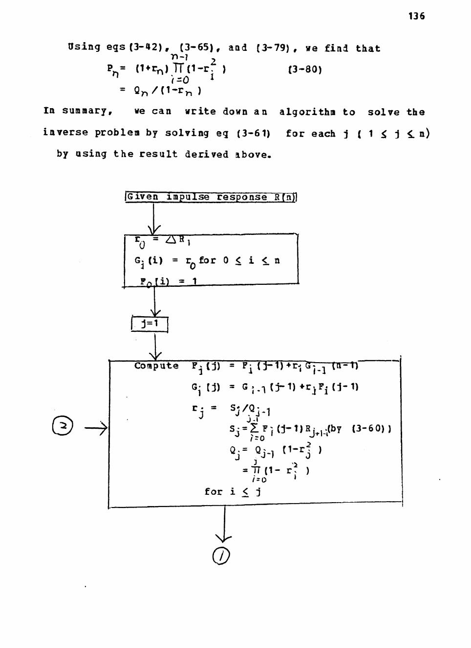
only 0(N ) multiplications^ The above procedure is written
as an algorithi as follows
I given R (t) j
^
^rrii
V i n v e r t i n g 2 by 2 matrix
hR 1
hR^ 1 raquo hR2
^ ^
Computing K(nm)
-n lt m lt n
V Q = P bull 1J
T Coifut ing
Scalar 1 = 1 hBgty2
Couputmg
t =
plusmn V
B B_2 bull^2n
-1
89
copy-
Computing 01
y = 1
- X bull Scalar 1
computing
Z == I hR-j bull (C 0
hR^
1) Y
hRin
regf NC
_Q Assigning INV to the
inversed central block
of 2(n1) by 2|n1) matrix
which is to be inverted
next
plusmn Computing
K (nm)
yES y
)
90
computation ror
impedance Z(^)
Besides using the trapezoid rule ve may incopcrate
Simpsons 13 rule and Simpsons 38 rule to approximate the
Gelfand-Levitan equation so that the truncation error is
improved By combining Simpsons 13 rule and the trapezoid
rule together we can find another matrix formulation
corresponding to this
91
I bull h
0
0
0
0
0 bull bull bull 0
0 c
0 bull bull 0
0 bull (43)R^
0
0
laquo 1
(23) B^
0
(V3)B^
laquo ^
(V3)f l3
M (56) B
laquo3 (56) R
1
R i ^ B an-4 in3 2h-2 R gtn-1
l |^CV3)B^ (23) R^^ (V3)R^^j23)R^^^(43)R^^ f56) R^^
7 [hk (n-n1)l
hk (n-E2)
hk (n-nlaquo-3)
hk (n-E+4)
hk (n-n+5)
hk (nn-1)
Jhk(En)
(1-56)ha-j
0
(1-56)hB^
0
0
0
0
0
(1-56) hR^J 1
0
(3-24)
Equ (2-24) locks a little complicated and loses its beauty
and symmetry We thus need to modify the previous algorithm
to fit (3-24) Me can not use the inverted matrix obtained
92
a t the previous s t a g e as the i n v e r s e block to save the labor
of i n v e r t i n g the current matrix I n s t e a d we have t o s t a r t
from i n v e r t i n g a 2 by 2 matrix which i s the c e n t r a l 2 by 2
matrix of the current 2n by 2n matrix and then fo l low the
same procedure as the previous algorithm does to expand and
i n v e r t the matrix with increas ing d i i e n s i o n s u n t i l we obtain
the i n v e r s e of the 2n by 2n matrix This modified algorithm
takes m u l t i p l i c a t i o n s of order 0 (2 + 4 bull bull bull bull bull bull n ) t o inver t
an n by n matrix (n even number) compared with previouus
one i e 0 (n ) bull Therefore using ( 2 - 2 4 ) we improve the
accuracy but lose the e f f i c i e n c y ^ In order to improve
accuracy f u r t h e r we may incorporate Simpsons 3 8 ru le i n t o
(3-24) by r e p l a c i n g four-point i n t e g r a t i o n with S iapson s
3 8 r u l e ins tead of the method used be fore The matrix
formulation for t h i s i s l i s t e d as f o l l o w s
I bull h
N
0
0
0
0
0
0 bull bull
0 bull
0
0 bull bull
0
0
c
c
c
1 1
0
0
0
4Rj
R
R 1 0 0
0 B-j3 5R26
9R-I8 9R^8 7H^8
4Rj3 2R^3 ^B33 5R^6
Ra R 4 ^S
0 bull bull9R^a 9B28 3R34 9fl^4 9R^V8 7B^8
I
93
hk(n-i1)
hk(n-n2)
hk(n-n3)
hk(n-c4)
Uhk(nc)
(1-56)hR^
(1-78)hR^
(1-56)hR
+
0
0
0
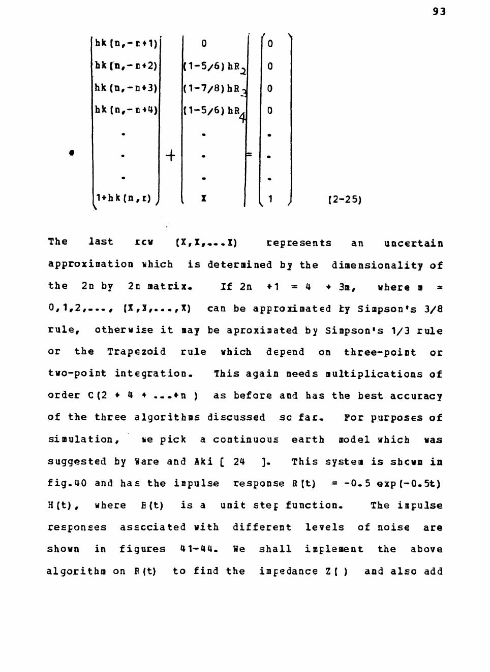
I (2-25)
The last rcw (XXX) represents an uncertain
approximation vhich is determined by the dimensionality of
the 2n by 2n matrix If 2n +1 = 4 bull 3m where m =
012 IyX) can be approximated by Simpsons 38
rule otherwise it may be aproximated by Simpsons 13 rule
or the Trapezoid rule which depend on three-point or
two-point integration This again needs nultiplications of
order 0(2 bull 4 + bullbulln ) as before and has the best accuracy
of the three algorithms discussed so far For purposes of
simulation ve pick a continuous earth model which was
suggested by laquoare and Aki [ 24 ] This system is shewn in
fig40 and has the iipulse response fl (t) = -05 exp(-0^5t)
H(t) where B (t) is a unit step function^ The ispulse
responses associated with different levels of noise are
shown in figures 41-44 We shall implement the above
algorithm on B (t) to find the impedance Z( ) and also add
to R (t) for comparison The
simulation results are listed as fellows
Multiplications
to invert
Approi rules Variance of noise n by n matrix Result
Trapezoid
same
same
same
same
sameuro
Sinpson 13
Irapezcid
same
same
same
same
same
Siirpson 13
33
Trapezoid
same
same
same
No
0000001
000001
0OCO1
0001
0-01
Nc
0000001
00C001
00001
0001
001
No
CCCOOOI
C00001
00001
C(n^)
same
same
sane
same
same
Table
Table
Table
Table
Table
Table
13
14
15
16
17
18
C(2 +4 bulla )
same
same
same
same
same
same
same
same
same
Table 19
Table 20
Table 21
Table 22
Table 23
Table 24
Table 25
Table 26
Table 27
Table 28
95
same 0001 same Table 29
sane 001 same Table 30
96
Impedance Z( F )
Travel time
i gu re 40 The s imula ted ea r th model with cont inuous impedance
97
Figure 41 The impulse response of the system in fig40 with no noise corrupton
Figure 42 The Noisy impulse response of the system in fig40 (rx = o 000001)
n
98
Figure 43 The noisy impulse response of the system in figiO(o^ = 000001)
Figure 44 The noisy impulse response of the system fig-^0 (c = 00001)
ID
100
TABLE 13
Approximation rule Trapezoid Noise Ch = 0 n
ZK
Z( 7 A V
Z( Z( Z( Z( Z( Z( Z( Z( Z( Z( Z( Z( Z( Z( Z( Z( Z( zlt Z( Z( Z( Z( Z( Z( Z( Z( Z( Z ( Z( Z( Z( Z( Z( zlt Z( 7
Z(
005000 ) 010000 ) 015000 gt 020000 ) 025000 ) 030000 ) 035000 ) 040000 ) 045000 gt 050000 ) 055000 ) 060000 gt 065000 ) 070000 ) 075000 gt 080000 ) 085000 ) 090000 gt 095000 ) 100000 ) 105000 ) 110000 ) 115000 ) 120000 ) 125000 ) 130000 ) 135000 gt 140000 ) 145000 ) 150000 ) 155000 ) 160000 ) 165000 ) 170000 ) 175000 ) 180000 ) 185000 ) 190000 ) 195000 ) 200000 )
010379788E+01 ERROR 010886448E+01 ERROR 011393454E+01 ERROR 011900823E-I-01 ERROR 012403571E+01 ERROR 012916714E+01 ERROR 013425269E+01 ERROR 013934 253E--01 ERROR 014443683E+01 ERROR 014953574E+01 ERROR 015463944E+01 ERROR 015974809E+01 ERROR 0164861S7E+01 ERROR 016998095E+01 ERROR 017510543E+01 ERROR 018023565E+01 ERROR 0raquo18537163E+01 ERROR 0gt19051358E+01 ERROR 0i9566169E+01 ERROR 020081612E+01 ERROR 020597705E+01 ERROR 021114466E+01 ERROR 021631912E+01 ERROR 022150061E+01 ERROR 022668930E+01 ERROR 0raquo23138533E-I-01 ERROR 023708904E+01 ERROR 024230043E-f01 ERROR 024751976E+01 ERROR 025274721E+01 ERROR 025798295E+01 ERROR 026322713E-f0i ERROR 026848007E+01 ERROR 027374183E+01 ERROR 027901263E+01 ERROR 028429267E+01 ERROR 028953214E+01 ERROR 029483124E+01 ERROR 030019014E+01 ERROR 030550906E+01 ERROR
0 0 1 1 4 4 3 8 0 0 1 0 3 2 2 9 0 0 0 9 2 6 4 9 0 0 0 3 2 6 4 3 0 0 0 7 3 1 4 4 0 0 0 6 4 0 6 6 0 0 0 5 5 3 5 6 0 0 0 4 6 9 6 2 0 0 0 3 8 8 4 0 0 0 0 3 0 9 5 1 0 0 0 2 3 2 6 2 0 0 0 1 5 7 4 4 0 0 0 0 3 3 7 2 0 0 0 0 1 1 2 1
bull gtJ ltbull J 0J 6J 2 o
bull 0 0 0 1 3 0 9 2 bull 0 0 0 2 0 0 8 3 bull 0 0 0 2 7 0 3 0 bull 0 0 0 3 3 9 3 3 bull 0 0 0 4 0 3 0 6 bull 0 0 0 4 7 6 6 1 bull 0 0 0 5 4 5 0 7 bull 0 0 0 6 1 3 5 4 bull 0 0 0 6 3 2 0 9 bull 0 0 0 7 5 0 3 0 bull 0 0 0 3 1 9 7 3 bull 0 0 0 8 3 8 9 5 bull 0 0 0 9 5 3 5 2 bull 0 0 1 0 2 8 4 7 bull 0 0 1 0 9 3 3 8 - 0 0 1 1 6 9 7 8 - 0 0 1 2 4 1 2 2 - 0 0 1 3 1 3 2 4 bull 0 0 1 3 3 5 3 6 bull 0 0 1 4 5 9 1 4 - 0 0 1 5 3 3 1 0 bull 0 0 1 6 0 7 7 7 - 0 0 1 6 3 3 1 9 bull 0 0 1 7 5 9 3 ^ - 0 0 1 3 3 6 3
101
TABLE 14
Approximation rule Trapezoid Noise CN =0 00000 1 n
T 1 A H V
Z( Z( Z( Z( Z( Z( Z( Z(
Z( Z( Z(
Z( Z(
Z( Z( Z( Z( Z( Z( Z( Z( Z( Z( Z( Z(
zlt mdashraquo
i 1
Z ( Z( Z( Z( Z( Z( Z( Z( Z(
Z(
005000 ) 010000 ) 015000 gt 020000 ) 025000 ) 030000 ) 035000 ) 040000 ) 045000 ) 050000 ) 055000 ) 060000 ) 065000 ) 070000 ) 075000 ) 030000 ) 085000 ) 090000 ) 095000 ) 100000 ) 105000 ) 110000 ) 115000 ) 120000 gt 125000 ) 130000 ) 135000 ) 140000 ) 145000 ) 150000 ) 155000 ) 160000 ) 165000 ) 170000 ) 175000 ) 130000 ) 185000 ) 190000 ) 195000 ) 200000 )
0lt 10379689E-I-01 010835756E-f01 01139344eE-f-01 0raquo11900300E-I-01 012407888E--01 012916517E--01 013425017E-f-01 013933071E+01 014443325E-I-01 0gt14952879E-I-01 015464050E-^01 015975310E+01 016436408E+01 016993713E-F01 017510439E-f01 018024655E--01 01S537434E+01 019050311E-f01 019564450E-I-01 020073990E-f01 020593402E-J-01 021108063E-I-01 021624204E+01 022142531E-I-01 022662021E-^01 023132153E-1-01 023704852E+01 024225697E-f01 024745462E-I-01 025266904E-f01 025791942E-I-01 026313418E-f01 026845285E-h01 027372626E-f-01 027898493E-I-01 028425225E-I-01 023953S61E--01 029484056E-h01 030014625E--01 030547804E-I-01
ERROR ERROR ERROR
ERROR ERROR ERROR ERROR ERROR-
ERROR ERROR ERROR ERROR
ERROR ERROR ERROR ERROR ERROR ERROR ERROR ERROR ERROR ERROR ERROR ERROR ERROR ERROR
ERROR ERROR ERROR ERROR ERROR ERROR ERROR ERROR ERROR
ERROR ERROR ERROR ERROR ERROR
=
=
r
=
=
=
=
=
=
=
=
=
=
=
=
=
=
=
=
=
=
=
=
=
=
=
=
=
=
=
=
=
=
=
=
=
=
=
=
=
0 0 J
J
0 0lt 0lt 0lt 0 0-0 0
0 0
-0 -0 -0
-olt -olt - 0 - 0 - 0 -0lt - 0 - 0
- 0 - 0 - 0 - 0 - 0 - 0 - 0 - 0 -0 lt
-bullJ
-0 -0 -0
bull 011^1532 bull0103353 0092654 0032667 0073690 0064213 0055543 0047306 ^0039086 ^0031414 0023194 0015432 0008238 0000754 0005965 0013697 0020234 0026479 0033051 0039495 0045562 0051461 0057769 0064787 0072010 0079199 0037171 0094040 0100183 0106762 0114437 0122468 0130296 0133009 0144906 0151366 0159249 0166916 0174449 0182601
TABLE 15
Approximation rule Trapezoid Noise (^ =000001
102
Zlt zc Z( Z( zlt Z( Z( Z( Z( Z( Z( Z( Z( Z( Z( 2(
Z( Z( Z( Z( Z( Z( Z( Z( Z( 7(
Z( Z( Z(
Z( Z( Z( Z(
005000 010000 015000 020000 025000 030000 035000 040000 045000 bull50000 55000
0 0 0 KJ
0 J
0 0 0 0 1 1 1 1 1 1 1 1 1 1 1 4
1
1 1 1 1 1 1 1 1 2
60000 65000 70000 75000 80000 85000 90000 95000 bull00000 05000 bull10000 bull15000 bull20000 bull25000 bull30000 bull35000 bull40000 bull45000 bull50000 55000 bull60000 bull65000 bull70000 75000 bull80000 bull35000 bull90000 bull95000 ) = bull00000 ) =
0^10379475E--01 0 10834261E-I-01 011393437E+01 011900750E-I-01 012406411E--01 012916092E-f01 013424471E-i-01 013930516E-f01 014442552E+01 014951376E-f01 015464278E-i-01 015976391E-f01 0164868S6E-I-01 017000067E-f01 0lt 17510203E-f-01 018027012pound-H01 0lS533020E--01 019043046E-I-01 0 19560734E-1-01 0gt20073324E+01 020534102E-f-01 021094242E--01 021607550E+01 022126261E+01 022647094E-h01 0bull23168372E-^01 023696098E-I-01 0^24216306E-h01 0^24731387E-I-01 0^25250016pound-H01 0^25773217E+01 0^26309132E+01 026839407E-f01 027369267E-)-01 027392512E-1-01 028416495E-i^01 028944460E-1-01 029475274E-^01 030005143E--01 030541109E-i-01
ERROR ERROR ERROR ERROR ERROR ERROR ERROR ERROR ERROR ERROR ERROR ERROR ERROR ERROR ERROR ERROR ERROR ERROR ERROR ERROR ERROR ERROR ERROR ERROR ERROR ERROR ERROR ERROR ERROR ERROR ERROR E R R 0 R ERROR ERROR ERROR ERROR ERROR ERROR ERROR ERROR
=
=
=
=
=
=
=
=
=
=
=
=
=
=
=
=
=
=
=
=
=
=
=
=
=
=
=
=
=
=
=
=
=
=
=
=
=
=
= bull
=
0 0 0 0lt 0 0 0 0 0 KJ
0 0 0
-0 -0 -0 -0 -0lt -0lt -0
-0 -0 -0 -0 -0lt -0lt -0 -0lt -0 -0 -0lt -0 -0 -0 -0 -0 -J
-0 -0
0114736
0105213
0092664
0032709
0074371
0064544
0055947
0049631
0039619
0032416
0023046
0014756 0007943 0000040 0005830 0015006 0020551 0025237 0031146 0036662 0041025 0044877 0050023 0057391 0065375 0073205 0033446 0090128 0094443 0100007 0109105 0113397 0128073 0136766 0142732 0148743 0155951 0163388 0171236 0180370
TABLE 16
Approximation rule Trapezoid Noise o =00001 0
103
Z( 005000 ) = Z( 010000 gt -Z( 015000 ) = Zlt 020000 ) -Z( 025000 ) = Z( 030000 ) = Z( 035000 ) = Z( 040000 ) = Zlt 045000 ) = Z( 050000 ) = Z( 055000 ) = Z( 060000 ) = Z( 065000 ) = Z( 070000 ) = Z( 075000 gt = Z( 030000 ) -Z( 085000 ) = Z( 090000 ) = Z( 095000 ) = Z( 100000 ) = Z( 105000 ) = Z( 110000 ) -Z( 115000 ) = Z( 120000 ) = Z( i25000 ) = Z( 130000 ) = Z( 135000 ) = Z( 140000 ) = Z( 145000 ) = Z( 150000 ) = Z( 155000 ) = Z( 160000 ) = Z( 165000 ) = Z( 170000 ) = Z( 175000 ) = Z( 180000 ) = Z( 185000 ) = Z( 190000 ) bull-Z( 195000 ) = Z( 200000 ) =
010378799E-I-01 ERROR 010879534E-r01 ERROR 011393399E-J-01 ERROR 011900592E-I-01 ERROR 012401743E+01 ERROR 012914749E-I-01 ERROR 013422747E-f01 ERROR 013922440E+01 ERROR 014440110E+01 ERROR 014946625E-f01 ERROR 0raquo15465005E-J-01 ERROR 015979314E-I-01 ERROR 0164S3399E+01 ERROR 017004336E-f01 ERROR 017509459E-f01 ERROR 018034463E-f01 ERROR 0lS539876E-f01 ERROR 019040390E^f01 ERROR 019548990E-f01 ERROR 020055420E-5^01 ERROR 020554727E-f01 ERROR 021050592E^f01 ERROR 021554986Ebull^01 ERROR 022074916E-f-01 ERROR 022599936E-1-01 ERROR 023121372E-i-01 ERROR 023668481E+01 ERROR 024136677E-I-01 ERROR 024686930E+01 ERROR 025196743E+01 ERROR 025734925E+01 ERROR 026279856E-i-01 ERROR 026320902E-raquo-01 ERROR 027353730E-l-0i ERROR 027873694E+01 ERROR 023383996E-f01 ERROR 028914843E+01 ERROR 029447615E--01 ERROR 029975294E+01 ERROR 030520044E+01 ERROR
00115430 00109515 00092696 00032340 00078605 00065573 00057224 00055400 00041304 00035533 00022573 00012617 00007031
-00002551 -00005405 -00019149 -00021555 -00021521 -0lt 0025123 -00027710 -00026696 -00024091 -00025575 -00034053 -00044438 -00054292 -00071694 -00077782 -00076313 -00073697 -00092127 -00107637 -00121095 -00132363 -00135389 -00133927 -00145559 -00154350 -00161117 -00173348
104
TABLE 17
ApproxiiBation rule Trapezoid Noisei o =0001
Z( zlt Z( Z( 2lt Z( Z( Z( Z( z-( 2( Z( Z( Z( Z( Z( zlt Z( Zlt Z( Zlt Z( Z( Z( Z( Z( Z( zlt Z( Z( Z( Z( Z( Z( Z( Z( Z( Z( z- Z(
005000 ) 010000 ) 015000 ) 020000 ) 025000 ) 030000 ) 035000 ) 040000 ) 045000 ) 050000 ) 055000 ) 060000 gt 065000 ) 070000 gt 075000 ) 080000 ) 085000 ) 090000 ) 095000 ) 100000 ) 105000 ) 110000 gt 115000 ) 120000 ) 125000 ) 130000 ) 135000 ) 140000 ) 145000 gt 150000 ) 155000 ) 160000 ) 165000 ) 170000 ) 175000 ) 180000 ) 185000 ) 190000 ) 195000 ) 200000 )
0 10376663Ebull^01 ERROR 010364603E-h01 ERROR 011393284E-1-01 ERROR 0 gt11900096E-I-01 ERROR 012386997E-F01 ERROR 012910504E-I-01 ERROR 013417303E--01 ERROR 0 1389694 4 E-l-01 ERROR 014432395E-i-01 ERROR 014931619E-f-01 ERROR 015467336E-1-01 ERROR 015990650E^f01 ERROR 016493195E-1-01 ERROR 017017362E-I-01 ERROR 017507115E-I-01 ERROR 018058032E-i-01 ERROR 0 18545766E-f 01 ERROR 019018306E-f-01 ERROR 019511927E-f01 ERROR 019998954E-h01 ERROR 020462166E+01 ERROR 020913249E-I-01 ERROR 021339769E--01 ERROR 021913577E+01 ERROR 02245i972E-^01 ERROR 022983232E-f01 ERROR 023581730E--01 ERROR 024093652E-I-01 ERROR 024547566E-^01 ERROR 025029553E-f01 ERROR 0^2559910SE+01 ERROR 0^26188178E-f01 ERROR 026763199E-i-01 ERROR 0raquo27326235E--01 ERROR 0raquo27815104E-I-01 ERROR 028303087E+01 ERROR 023322283E-I-01 ERROR 029361252E-I-01 ERROR 0 29882036E+ 01 ERROR 030454502E-I-01 ERROR
00117464 00123088 0^0092797 00083254 00090402 00068343 00061257 00073612 00046624 00045587 0 0021074 00005844 00004125 00010507 00004066 00032268 00024738 00009634 00006116 00000523 00018456 00041310 00051270 00039233 00021346 00005117 00034800 00039022
= -00019414 = -00011323 = -00038866 = -00072376 = -00099320 = -00120827 = -00114583 = -00103245 = -00113082 = -00124570 = -00129504 = -00151501
ZZ mdash I
TABLE 18
Approximation rule Trapezoid Noise Oi =001
105
Z( Z( Z( Z( Z( Z( Z( zlt Z( zlt zlt Z( Z ( Z( Z( Z( Z( Z( zlt Z( Zlt Z( X
z
L
Z( zlt Z( Z( Z( Z( Z( Z( Z( Z( zlt Z( Z(
005000 010000 015000 020000 025000 030000 035000 040000 045000 050000 055000 060000 065000 070000 075000 080000 085000 090000 095000 100000 105000 110000 115000 120000 125000 130000 135000 140000 145000 150000 155000
160000 165000 170000 175000 180000 185000 1 90000 195000 200000
0 0 0 0 0 0 0laquo 0 Oi
0 0 0 0 0 0 0 0 0 0 0 0 0 0 0 0 0 0 0 0 0 0laquo 0 0 0 0 0 0 0 0 0
10369918E+01 10817556E-I-01 11392939E-r01 11893546E-i-01 12340511E+01 12897132E-f01 13400181E-f01 13816727E^f01 14408113E-f01 14884343E+01 15475045E+01 16025031E+01 16508474E-I-01 17060935E-f01 17499789E-I-01 13133131E-f-01 18564593ET01 18947321E-I-01 19395459E-i-01 19821339E-)-01 20172649E+01 20485721E-f01 20877012E+01 21413382E-^01 21993124E+01 22565020E-i-01 23313863ET01 23306019E-1-01 24116661E-h01 21513374E-f01 25180300E-I-01 25907243E-f01 26538990E-I-01 27232065E-f01 27639138E-I-01 23041946E-I-01 28540326E-J-01 29099043E^f01 29598452E-f-01 30257940E-h01
E = R 0 R raquomdash bull-bull - r
c rv U Pi ERROR ERROR ERROR ERROR ERROR ERROR ERROR ERROR ERROR ERROR ERROR ERROR ERROR ERROR ERROR ERROR ERROR ERROR ERROR ERROR ERROR ERROR ERROR ERROR ERROR ERROR ERROR ERROR ERROR ERROR ERROR ERROR ERROR ERROR E R R 0 R ERROR ERROR ERROR
00123837 00165353
00034545 00127591 00079129 00073940 00130909 00063370 00077102 00016100 bull00015676 bull00005136 bull00035344 00000121 bull00073962 bull00034915 00027726 00053611 00039056 00159684 00244395 00289762 00266645 00225273 00189122 00079207 00080325 00156465 00194650 00125373 00035674 -00033531 bull00085950 bull00050614 -00014930 bull00014149 bull00034153 bull00033373 -00035980
106
TABLE 19
Approx rules Trapezoid and Simpson 13 Noise o =0 000001
Z( Z( Z( Z( Z( Z( Z( Z( Z( 11 If
Z( Z( Z( Z( Z( Z( Z( Z( Z( Zlt Z( Z( Z( Z( Z( Z( Z( zlt Z( Z( z- Z( Z( zlt Z( Z( Z( Z(
005000 ) 010000 ) 015000 ) 020000 ) 025000 ) 030000 ) 035000 ) 040000 ) 045000 ) 050000 ) 055000 ) 060000 ) 065000 gt 070000 ) 075000 ) 080000 ) 085000 ) 090000 ) 095000 ) 100000 ) 105000 ) 110000 ) 115000 ) 120000 ) 125000 ) 130000 ) 135000 ) 140000 gt 145000 ) 150000 ) 155000 ) 160000 ) 165000 ) 170000 ) 175000 ) 180000 ) 135000 ) 190000 ) 195000 ) 2^00000 )
0^10534874E--01 ERROR 0^10931243E-I-01 ERROR 011439001E--01 ERROR 0raquo11947337E-I-01 ERROR 012456002E--01 ERROR 012965232E-I-01 ERROR 013474829E+01 ERROR 013935079E-h01 ERROR 014495635Ef01 ERROR 015006932E-I-01 ERROR 015518572E-f-01 ERROR 016030993E+01 ERROR 016543796E-J-01 ERROR 017057419E--01 ERROR 017571462E-i-01 ERROR 018036365E-f-01 ERROR 018601728E+01 ERROR 019117991E-i01 ERROR 019634754E-i-01 ERROR 020152457E+01 ERROR 020670700E+01 ERROR 021189924E-t-01 ERROR 021709729E+01 ERROR 022230556E-h01 ERROR 022752005E-i-01 ERROR 023274518E-f01 ERROR 023797695E-I-01 ERROR 024321979E-I-01 ERROR 024346968E-|-01 ERROR 025373107E-f-01 ERROR 025899994E-i-01 ERROR 026428075E-e01 ERROR 0raquo26956947E-h01 ERROR 027487057E-I-01 ERROR 028018002E+01 ERROR 0raquo23550230E-I-01 ERROR 029083338E-i-01 ERROR 0^29617775E-I-01 ERROR 0^30153136E-I-01 ERROR 030689872E-I-01 ERROR
-00033214 00062507 00053043 00043844 00035199 00026706 00018645 00010653 00003011
-00004621 -00011982 -00019370 -00026543 -00033776 -00040835 -00047981 -00054988 -00062101 -00069105 -00076229 -00033263 -0009 044 0 -00097543 -00104798 -00112002 -00119355 -00126679 -00134158 -00141619 -00149243 -00156860 -00164644 -00172433 -0^0130391 -0^0183364 -0^0196511 -00204680 -0^0213026 -00221402 -00229957
107
TABLE 20
Approx rules Trapezoid and Simpson 13 Noise (3 =0000001
Z( Z( zlt Z( Z( Z( Z( Z( Z( zlt Z( Z( Z( Z( Z( Z( Z( Z( z- 7 (
Z( 7 ( Am
Z( Z( Z( Z( Z( Z( Z( Z( Z( Z( zlt Z( Z( Z( Z( Z( Z( 7 (
005000 ) 010000 ) 015000 ) 020000 gt 025000 ) 030000 ) 035000 ) 040000 ) 045000 ) 050000 ) 055000 ) 060000 gt 065000 ) 070000 ) 075000 ) 080000 ) 085000 ) 090000 ) 095000 ) 100000 ) 105000 ) 110000 ) 115000 ) 120000 ) 125000 ) 130000 ) 135000 ) 140000 ) 145000 ) 150000 ) 155000 ) 160000 ) 165000 ) 170000 ) 175000 ) 180000 ) 185000 ) 190000 ) 195000 ) 200000 )
010534885E-^01 0 10930421E-f01 011438991E-f-01 011947344E-f01 012455066E-i-01 012965014E-I-01 013474790E-01 013983923E-I-01 0i4495275E-f01 015006153E-h01 015518330E-1-01 016030751E-I-01 0bull16543192Ebull^01 017057517E-I01 0 17570953E-1-01 018037351E-i-01 0lS601916E-)-01 019117261E^f01 019633761E-I-01 020151060E--01 020667775E-(-01 0211848l4E-5-01 021703305E-H01 022224341E--01 022746776E+01 023269759E-1-01 023795441E--01 024319571E-h01 024842737E-I-01 025367740E--01 025896388E--01 026426947E-h01 026957333E-I-01 027489080E-I-01 028019431E-h01 023551007E+01 029084227E-h01 029619126E-1-01 030134536E-h01 030692914E-I-01
ERROR = -0 r- r- rgt ft r- _ f
c r K U p - J
ERROR = 0 ERROR = 0 ERROR = 0 ERROR = 0 ERROR = 0 ERROR = 0 ERROR = 0 ERROR = -0 ERROR = -0 ERROR = -0 ERROR = -0 ERROR = -0 ERROR = -0 ERROR = -0 ERROR = -0 ERROR = -0 ERROR = -0 ERROR = -0 ERROR = -0 ERROR = -0 ERROR= -0 ERROR = -0 ERROR = -0 ERROR = -0 ERROR = -0 ERROR = -0 ERROR = -0 ERROR = -0 ERROR = -0 ERROR = -0 ERROR = -0 ERROR = -0 ERROR = -0 ERROR = -0 ERROR = -0 ERROR = -0 ERROR = -0 ERROR = -0
0033224 0063254 0053051 0043380 0035947 0026912 0018674 0011433 00 00 00 00 00 00 00 00 00 00 00 00 00 00 00 01 01 01 01 01 01 01 01 01 01 01 01 01 02
02 02 02
A T e lt-raquo
0 i w 7
04105 11826 19219 26177 33834 40545 43523 J laquo_ U O 7
61716 68596 75530 81341 38007 94560 01973 09678 17286 25719 33155 39913 47096 55446 64210 72579 81140 83334 96788 04992 13492 21876 30971
108
TABLE 21
Approx r u l e s Trapezoid and Simpson 13 Noise (5 ^ = 000001
Z( Z( Z( Z( Z( Z( Z( Zlt Z( Z( Z( Z( zlt Z( Z( Z( Z( Z( Z( Z( Z( Z( Z( zlt Z( zlt Z( Z( Z( Z( Z( Z( Z( Z( Z( Z( Z( Z( zlt Z(
005000 ) 010000 ) 015000 ) 020000 ) 025000 ) 030000 ) 035000 ) 040000 ) 045000 gt 050000 ) 055000 ) 060000 gt 065000 ) 070000 ) 075000 ) 030000 ) 085000 ) 090000 ) 095000 ) 100000 ) 105000 ) 110000 ) 115000 ) 120000 ) 125000 ) 130000 ) 135000 ) 140000 gt 145000 ) 150000 gt 155000 ) 160000 ) 165000 A 170000 gt 175000 ) 180000 ) 185000 ) 190000 ) 195000 ) 200000 )
010534907E-F01 ERROR 010928643E-)-01 ERROR 01143S970E+01 ERROR 011947252Ebull^01 ERROR 012453044E-I-01 ERROR 012964435E-h01 ERROR 013474706E-01 ERROR 013981424E-I-01 ERROR 014494497E-I-01 ERROR 015004485E-F01 ERROR 015517S08E--01 ERROR 016030223E-I-01 ERROR 01654i888E-l-01 ERROR 017037731E-^01 ERROR 017569854E-r01 ERROR 013089483E-I-01 ERROR 018602321E+01 ERROR 019115683E-f01 ERROR 019631614E-h01 ERROR 020143037E-I-01 ERROR 020661451E-i-01 ERROR 021173771E-I-01 ERROR 021689422E-h01 ERROR 022210911E-H01 ERROR 022735476E-H01 ERROR 023259474E-i-01 ERROR 023790570E-r01 ERROR 024314368E^i-01 ERROR 024833753E-^01 ERROR 025356142E-f-01 ERROR 0 25888596E-h01 ERROR 026424510E-^01 ERROR 026958172E-h01 ERROR 027493455E-i-01 ERROR 028022521E+01 ERROR 028552684E+01 ERROR 0 29086147E-t-01 ERROR 029622046E-f01 ERROR 030157562E-I-01 ERROR 030699488E-I-01 ERROR
gtj
J 0
-00033245 00064370
0053069 004 39 57 0037565
00027353 00018736 00013263 00003795
-00002990 -00011489 -00018892 -00025336 -00033960 -00039917 -00049713 -00055309 -00060836 -00067495 -00074019 -00073756 -00082743 -00033103 -00095863 -00104656 -00112814 -00123646 -00130937 -00136226 -00142457 -00152390 -00163273 -00172895 -00182761
0190008 -00197387 -00205666 -00214499 -00222902 -00233163
= - K J
109
TABLE 22
Approx rules Trapezoid and Simpson 13 Noise (^=00001
zlt Z( Z( Z( Z( Z( Z( Z( L K
Z( zlt zlt Z( Z( Z( Z( Z ( Z( Z( Z( Z( Z( zlt Z( Z( Z( Z( Z( Z( Z( z- zlt Z( Z( Z( Z( Z( Z( Z( Z(
0 0 0 0 0 0 0lt 0 0 0 0 0 0 0 0 0 0 0 0 1 1 1 1 1 1 1 1 1 1 1 1 1 1 1 1 1 1 1 1 -V
05000 10000 15000 20000 25000 30000 35000 40000 bull45000 50000 55000 60000 65000 70000 75000 80000 85000 90000 95000 00000 05000 10000 15000 20000 25000 30000 35000 40000 45000 50000 55000 60000 65000 70000 75000 30000 85000 90000 95000 00000
010534979E+01 ERROR 010923024E-I-01 ERROR 011438904E-1-01 ERROR 011946960E-F01 ERROR 012446650E--01 ERROR 012962604E-f01 ERROR 013474440E-^01 ERROR 013973526E-I-01 ERROR 014492039E-f01 ERROR 014999197E-f-01 ERROR 015516157E+01 ERROR 016023571E-f01 ERROR 016537759E+01 ERROR 017053408E-^01 ERROR 017566378E--0i ERROR 018096230E+01 ERROR 0 lS603605E-f01 ERROR 019110694E-f01 ERROR 019624826Ef-01 ERROR 020138477E-I-01 ERROR 020641465E--01 ERROR 021138392E-I-01 ERROR 021645594E-f01 ERROR 022168515E-h01 ERROR 022699800E+01 ERROR 023227005E^f01 ERROR 023775195E-^01 ERROR 024297943E-)-01 ERROR 024S0522SE-)-01 ERROR 025319529E-J-01 ERROR 025S63995E-f01 ERROR 026416821E^f01 ERROR 026960842E+01 ERROR 027507307E-^01 ERROR 028032292E--01 ERROR 023557973E-F01 ERROR 029092197E-f01 ERROR 029631264E-I-01 ERROR 030167108E-I-01 ERROR 030720257E-I-01 ERROR
-00033313 00069973 00053127 00044200 00042680 00028766 00018933 00018910 00005490 00000535
-00010424 -00017357 -00022884 -00034353 -00037930 -00053461 -00056002 -00053260 -00064013 -00069239 -00069007 -00066139 -00067718 -00076593 -00088300 -00093693 -00117104 -00124143 -00124533 -00127312 -00142743 -00160316 -00173903 -00137391 -00193561 -00199276 -00207789 -00217677 -00226138 -00240086
110
TABLE 23
Approx rules Trapezoid and Simpson 13 Noise (gt =0-001
Z( Z( Z( Z( Z( Z( Z( 2 Z( Z( Zlt Z( Z( Z( Z( Z( Z( Z( Z( Z( zlt Z( Z( Z( Z( Z( Z( Z( Z( Z( Z( Z( Z( zlt Z( Z( Z( Z( Z( Z(
005000 ) 010000 ) 015000 ) 020000 ) 025000 ) 030000 ) 035000 ) 040000 ) 045000 ) 050000 ) 055000 ) 060000 ) 065000 ) 070000 gt 075000 ) 080000 ) 085000 ) 090000 ) 095000 ) 100000 ) 105000 ) 110000 ) 115000 ) 120000 ) 125000 ) 130000 ) 135000 ) 140000 ) 145000 ) 150000 ) 155000 ) 160000 ) 165000 ) 170000 ) 175000 ) 180000 ) 185000 ) 190000 ) 195000 ) 200000 )
010535204E+01 ERROR 0gt10905272E-I-C1 ERROR 011438697E-f-01 ERROR 011946039E-^01 ERROR 012426444E+01 ERROR 012956319E+01 ERROR 013473603E--01 ERROR 013948592E-I-01 ERROR 014484278E-I-01 ERROR 0gt14982493E-f01 ERROR 015510951Ebull^01 ERROR 016023298E--01 ERROR 016524667E+01 ERROR 017060552E^f01 ERROR 017555392E--01 ERROR 018117597E-i-01 ERROR 018607631 E-l-01 ERROR 0gt19094939E-f01 ERROR 019603366E-I-01 ERROR 020108219E-f01 ERROR 020578371E--01 ERROR 021029037E-f01 ERROR 021507709E+01 ERROR 022035172E-f01 ERROR 022587541E-t-01 ERROR 023124880E-h01 ERROR 023726858E-I-01 ERROR 024 246279E-I-01 ERROR 024715455E-I-01 ERROR 025204354E-^01 ERROR 025786569E^f01 ERROR 02639 2668E-I-01 ERROR 026969476E-I-01 ERROR 027551261E-h01 ERROR 028063133E-h01 ERROR 028574550E--01 ERROR 029111115E-1-01 ERROR 029660250E-i-01 ERROR 030197072E-^01 ERROR 030785726E--01 ERROR
-00033528 00086117 00053307 00044963 00058345 00033216 00019553 00036720 00010843 00011672
-00007065 -00014561 -00014950 -00035619 -00031652 -00065332 -00058206 -00049963 -00053008 -00054110 -00033229 -00013827 -00003586 -00015937 -00033907 -00054295 -00096535 -00102616 -00037941 -00031741 -00112330 -00151026 -00177161 -00204171 -00204796 -00205196 -00214426 -00227672 -00236296 -00261909
Ill
TABLE 24
Approx rules Trapezoid and Simpson 13 Noise C5 =0-0
Z( Z( Z( Z( Z( Z( Z( Z( Z( Z( Z( zlt Z( zlt Z( Z( zlt Z( zc Zlt Z( Z( Z( Z( Z( Z( Z( Z( i K
Z( Z( Z( Z( Z( Z( Z( zlt Z( Z( Z(
005000 ) 010000 gt 015000 ) 020000 ) 025000 ) 030000 ) 035000 ) 040000 ) 045000 gt 050000 ) 055000 ) 060000 ) 065000 ) 070000 ) 075000 ) 080000 ) 085000 ) 090000 ) 095000 ) 100000 ) 105000 ) 110000 ) 115000 ) 120000 ) 125000 ) 130000 ) 135000 ) 140000 ) 145000 ) 150000 ) 155000 ) 160000 ) 165000 ) 170000 ) 175000 gt 180000 ) 185000 ) 190000 ) 195000 ) 200000 )
010535914E-I-01 ERROR 010349300E-f01 ERROR 011438074E+01 ERROR 011943154E-1-01 ERROR 012362663E+01 ERROR 012938598E-f01 ERROR 013470987E+01 ERROR 013870142E--01 ERROR 014459865E-i-01 ERROR 014929851E-I-01 ERROR 015494606E-^01 ERROR 016006311E-f01 ERROR 0164 82399E-h01 ERROR 017067415E-^01 ERROR 017520701E-^01 ERROR 0lS185553E-raquo-01 ERROR 018620764E+01 ERROR 019045334E-^01 ERROR 019535640E-I-01 ERROR 020012320E-I-01 ERROR 020379888E-I-01 ERROR 020686052E-f-01 ERROR 021073627E-f01 ERROR 021620673E-f01 ERROR 022238032E--01 ERROR 022307296E^f01 ERROR 023576953E--01 ERROR 024035679E+01 ERROR 0 244359 ISE-fOl ERROR 024846166E--01 ERROR 02554557SE+01 ERROR 026318245E+01 ERROR 026999068E-J-01 ERROR 027692440E-i-01 ERROR 028161475E-1-01 ERROR 023626116E-I-01 ERROR 029169266E-I-01 ERROR 029750343E-I-01 ERROR 030290228E-I-01 ERROR 030991504E-h01 ERROR
-00034204 00137000 00053849 00047372 00109366 00047232 00021491 00092756 00027680 00046766 00003430
-00003944 00010365
-00039656 -00011829 -00103035 -00065273 -00023860 -00013277 -00006160 00053591 00149499 00195937 00172421 00116430 00083735
-00032746 -00035700 00026156 00061533
-00017874 -00122402 -00138328 -00256459 -00240536 -00223613 -00234830 -00258912 -00267874 -00330501
TABLE 25
112
Approx r u l e s Trapezoid Simpson 13 and 38 Noise (V = 0
Zlt Z( Z( Z( zlt Z( Z( Z( Z( Z( Z( Z( Z( z- Z( Z( 7( Z( z- Z( Z( Z( L K
Z( Z( Z( Z( zlt Z( Z(
Z( Z( Z( Z( Z( 2 ( Z( Z( i K
0 0lt 0 0 0 0 0 0 0 0 0 0 KI
0
0
0 w
1 1 1 1 1 1 1 1 1 1 1 1 1 1 1 1 1 1 1 1 2
05000 )
10000 )
15000
20000
25000 ]
30000
35000 40000 45000 50000 bull55000 60000 65000 70000 7 5 0 J w
30000 85000 bull90000 95000 00000 05000 10000 15000 20000 25000 bull30000 35000 40000 45000 50000 55000 J 60000 bull65000 70000 75000 30000 85000 90000 95000 bull00000
=
-
=
) =
mdash
1 =
) =
gt =
) =
) =
gt =
) =
gt =
raquo -
gt =
) =
) ~
i =
1 =
bull -
1 =
1 =
1 =
1 =
1 ~
I =
gt =
1 =
= 1 mdash
mdash
1 =
=
1 =
1 z
) -
1 s
1 =
1 =
) mdash
0 0 0 0 0 0 0 0 0 0 0 0 0 0 0 0 0 0 0lt 0 0lt 0 0 0 0 0 0 0 0 0 0 0 0 0 0 0 KJ
0 0 0
10534874E-h01 10931843E-I-01 11439521E-F01 11943285E-f01 12457366E-f01 12966470E+01 13476871E-1-01 bull 13937959E-f01 14493356E^f01 bull 15010068Ebull^01 15522502E-I01 16034709Ebull^01 1654S535E--01 17063237E-I-01 17577006E^f01 13092452E-f01 18608969E-f01 bull 19124940E-J-01 19643018Ebull^01 bull 20162052E-t-01 20679S45Ebull^01 21199847E-f-01 21721202E+01 22241603E4-01 22764797E^f01 23283909E-f01 238113S3E-i-01 24336306E-I-01 24363780E-I-01 25389287E--01 25913509E-f-01 26448469E-5-01 26976294E-l-0i 27503048E-I-01 28041456E-^01 bull 23572758E-I-01 29108970E-I-01 29645536E-I-01 30179443E-1-01 30713493E-f01
ERROR ERROR ERROR ERROR ERROR ERROR ERROR ERROR ERROR ERROR
ERROR ERROR ERROR ERROR ERROR ERROR ERROR ERROR ERROR ERROR ERROR ERROR ERROR ERROR ERROR ERROR ERROR ERROR ERROR bullmdash Tl O r-
c r K u p ERROR ERROR ERROR ERROR ERROR ERROR ERROR ERROR ERROR ERROR
^
laquo
=
=
=
=
=
=
=
=
~
mdash
mdash
mdash
=
=
=
=
=
=
=
=
=
=
=
mdash
=
=
=
=
=
=
=
=
=
=
=
=
=
=
0 -0 -0 -0 -J
-0 -0 -0 -0 0 0 0 0 J t f
J
0 0 0-0 0 0 0 0 0 0 0 0 0
0 0 0 0 0 0 0 0 0 0 J
0033214
0061956
0052590 bull0043095 0034107 bull0025793 bull0017133 bull0003601 0001134 bull0006712 0014517 0021693 0029415 0037193 0044003 0051362 0053902 0065753 0073342 0031026 0087729 0095165 0102835 0109320 0117638 0125612 0132503 0140336 0148431 0155715 0164121 0172433 0179734 0138166 0196393 0204556 0213673 0222616 0230319 0239493
113
TABLE 26
Approx rules Trapezoid Simpson 13 and 38 Gv =0000001
Noisei
Z( Z( Z( Z( Z( Z( Z( zlt Z( Z( Z( zlt zlt 7( Z( Z( zlt Z( Z( Z( zlt Z( 7( Z( Z-
zlt Z ( Z(
Z(
zlt zc Z( 2 ( Z( Z( Z( Z( Z(
0 0 bullJ
0 0 0 0 0 0 0 0 0 0 0 bullJ
0 J
0 1 1 1 1 1 bull 4 1 1 1 1 1 1 1 1 1 1 1 1 1 1 4i
bull05000 10000 15000 20000 25000 30000 35000 40000 45000 50000 55000 60000 bull65000 70000 75000 30000 85000 90000 95000 00000 bull05000 bull10000 15000 bull20000 25000 30000 35000 40000 45000 50000 55000 60000 65000 70000 bull75000 80000 85000 90000 95000 00000
010534885E-I-01 ERROR 010931022E-i-01 ERROR 011439519E--01 ERROR 011948248E+01 ERROR 012456443E+0i ERROR 012966254E-f-01 ERROR 013476S53E--01 ERROR 013986799E--01 ERROR 014498111E+01 ERROR 015009378E-f-01 ERROR 0155222S8E-f-01 ERROR 016034714E-I-01 ERROR 01654S182E-I-01 ERROR 017063439pound-l-01 ERROR 017576761E+01 ERROR 0gt13093739E-f-01 ERROR 013609279E-t-01 ERROR 019124562E-f01 ERROR 019642275E-i-01 ERROR 020160762E+01 ERROR 020677201E-I-01 ERROR 021195018E-J-01 ERROR 021714937E--01 ERROR 022235697E--01 ERROR 022759917E--01 ERROR 023284207E4-01 ERROR 0 2 3 8 0 9 5 4 9 E T 0 1 ERROR 024334805E-i-01 ERROR 024859669E-J-01 ERROR 025384212E--01 ERROR 025915340E-I-01 ERROR 026447353E-I-01 ERROR 026976834E-I-01 ERROR 027510659E-f-01 ERROR 028042717E-I-01 ERROR 028573394E-I-01 ERROR 029110176E+01 ERROR 029646556E--01 ERROR 0301S0646E+01 ERROR 030721647E-i-01 ERROR
00033224 -00062708 -00052593 -00043127 -00034345 -00025959 -00017146 -00009429 - J 0 w 1 3 J o
00006252 00014379 00021696 00029201 00037317 00043863 00052077 00059069 00065559 00072961 00080381 00086439 00092866 00099971 00107135 00115518 00123563 00131723 00139502 00146303 00153635 00162378 00172059 00179937 00139133 00197352 00204733 00214097 00222951 00230727 00240549
114
TABLE 27
Approx rules Trapezoid Simpson 13 and 38 Noise CDJ- =000001
Z( zlt Z( Z( Z( Z( Z( Zlt 2lt Z( Z( zlt z- Z( K
Z Z( Z( bull 1
Z( Z( Z( Z( Z( bull ^ bull
1
Z( 7
Z( 7
Z( Z( L K
Z( Z( 7 ( Z( Z( Z(
Z
005000 010000 015000 020000 025000 030000 035000 040000 045000 050000 055000 060000 065000 070000 075000 080000 085000 090000 095000 100000 1 05000 110000 115000 120000 1^25000 130000 135000 140000 145000 150000 155000 160000 165000 170000 175000 180000 185000 190000 195000 200000
)
)
)
)
)
)
)
gt
)
gt
t
)
gt
)
)
gt
)
)
gt
)
)
)
)
)
)
)
)
)
)
)
)
)
)
) 1
)
010534907E-f01 010929235E-i-01 011439513E-f-01 011948167E-I-01 012454449E-01 012965736E-f01 013476815E-i-01 0gt13984291E-f01 014497580E+01 015007385pound-t-01 015521S27E--01 016034725E-|-01 016547417E-I-01 017063876E+01 017576230E--01 013096521E-i-01 018609949E-h01 019123743E+01 0 19640668E-)-0i 020157973E-f-01 020671436E-h01 021184579E^f01 021701400E--01 022222932E-i-01 022749366E+01 023274043E^f01 023805586E--01 024330431E-I-01 024350786E-l-0i 025373244E-l-0i 025908489E--01 026444941E-I-01 026973004E-h01 027516303E--01 028045444E-^01 023574763E--01 029112780E-f-0i 029648655E-h0i 030183246E-i-01 030728460E--01
ERROR ERROR ERROR ERROR r~ - r-laquo- -I
L pgt K u r ERROR ERROR ERROR E R R 0 R ERROR ERROR E R R G R ERROR ERROR ERROR ERROR
ERROR ERROR ERROR ERROR ERROR ERROR ERROR r- n r r r- c r P _bull P
ERROR ERROR ERROR ERROR ERROR ERROR ERROR ERROR ERROR ERROR ERROR ERROR ERROR ERROR ERROR ERROR
=
=
=
=
=
=
=
=
= mdash
=
=
=
=
=
=
=
=
=
=
=
=
=
=
=
=
= -
=
=
=
=
=
=
=
=
=
=
=
=
0 -0 -0 -0 -0 -0 -0 -0
0 0 0 J
0 0 0 0
bull i
J
w I
J bull
0
bullJ
0 J
J
0 0 0 0 0 0 0 0 0 0 J
0033245 bull0064332 0052598 0043194 0036441 0026313 0017174 0011220 0001669 0005257 0014082 0021703 0023737 0037574 0043560 0053623 rgt 0 bull=bull -bull 4 3 gt V w ~ WJ A_
0 J O _ i O 0072137 0073937 bull f^ - i c- i
0037395 0093675 0101332 0110829 0119151 0130037 0137700 0143178 0149298 0160192 0171131 0180379 0191223 0198343 0205274 0215010 0223674 0231609 w 4 o 2 0
115
TABLE 28
Approx rules Trapezoid Simpson 13 and 33 Noise
O-n i _ =00001
Z( Z( Z( Z( Z( Z( Z( Z( Z( zlt il
Z ( i v T
JL K
i 1
Z(
bull7
K
Z( zlt Z( Z( Z( Z( Z( z - Z( Z( Z( 7 (
Z( 7 (
zlt z- Z( 7
Z(
0
0 0 0 0 0 0 0 0 0 0
0 0 0 0 0
4
1 1 1 1 1 1 1 1 1 1 1 1 1 1 1 1 At
1 1 1 4 H
bull05000 10000 bull15000 bull20000 bull25000 bull30000 bull35000 bull40000 bull45000 50000 55000 60000 bull o 5 V 0 J
70000
75000
30000
85000
90000
95000
00000 05000 10000 bull15000 20000 25000 30000 35000 40000 45000 50000 55000 60000 65000 70000 75000 80000 35000 bull90000 bull95000 00000
)
)
)
)
)
) )
)
)
)
)
) )
)
)
) ) V
) )
)
)
gt
gt )
gt
gt
)
)
gt )
=
=
=
=
=
=
= =
=
=
=
=
= =
=
= =
=
=
=
=
= =
=
= mdash
mdash
= =
=
= =
=
=
=
=
= =
=
=
0 0 0 0 0 0 0 0 0 0 0 0 J
0 0 0 0 0
0 0 0 0 0 0 0 0 0 0 0 0 0 0lt 0 0 0 0 0 0 0
10534979E-f-01 10923538E-f01 11439494pound--01 11947911E-f01 1244S143E-^01 12964306E-f01 13476696E-t-01 13976370E-f01 14495898E-t-01 15003163E-f01 15520376E+01 16034757E-f01 16544989E-J-01 a7065269E-i-01 17574551E-I-01 13105319E-I-01 18612081E-f01 19121143E-f01 19635574E-^01 20149162E-f01 20653410E^f01 21151594E-f01 2165S667E-I-01 22182623E-I-01 22716030E-r01 23241993E-f01 23793067E-I-01 24316805E-f01 24822749E-I-01 25338603E-i-01 25886835E-I-01 bull 26437341E-I-01 26981716E-J-01 27534132E-I-01 28054072E-1-01 bull 28579104E-I-01 29120967E--01 29655289E-I-01 30191448E-I-01 30749950E-I-01
ERROR ERROR ERROR ERROR ERROR ERROR ERROR ERROR ERROR ERROR ERROR ERROR ERROR ERROR ERROR ERROR ERROR ERROR ERROR ERROR ERROR ERROR ERROR ERROR ERROR ERROR ERROR ERROR ERROR ERROR ERROR ERROR ERROR ERROR ERROR ERROR ERROR ERROR ERROR ERROR
mdash
mdash
=
=
=
=
= =
=
=
=
=
= =
=
= =
=
=
=
= =
=
=
= s
-
= =
= =
=
=
=
=
=
= =
=
=
0 -0 -0 -0 -0 -0 -0 -0 -0 0 0 0 bullJ
0 0 0 0 0 0lt 0lt 0 0 0 0 0 0 0 0 0 0lt 0 0 0
0 0 0 0 V
KJ
V 0 J J-1 3 bull0069466 0052614 0043403 bull0041485 0027457 0017262 0016379 0002329 0002112 0013146 0021723 0 0 O o i T gt T -bull
J Q o i 7 o 004^0^1 0053510 0060534 0063762 0069525 0074531 0074834 0072183 0073799 0083010 0096013 0105214 -0124709 0132002 0131734 0135441 0151700 0168203 0181730 0197327 0201431 0206822 V 1 O O w
0225962 0234389 0249983
116
TABLE 29
Approx r u l e s Trapezoid Simpson 13 and 38 Noise
i _ =0001
Z K
Zlt L K
zlt z- zlt
Z z- Z(
005000 010000 015000 020000 025000 030000 035000 040000 045000 050000
)
)
)
)
)
)
) laquo
)
)
i K
7
Z( L K
Z( i K
Z( Z( 7( Z(
Z( L
ZK
JL K
Z(
7
055000 ) 060000 ) 065000 ) J 0 V J 0 J
bullJ 5 0 J 0
030000 ) 085000 ) 090000 gt 095000 ) 100000 ) 105000 gt 110000 ) 115000 ) 120000 ) 125000 130000 135000 1 40000 145000 150000 155000 160000 165000 170000 175000 1 30000
= ) ^
135000 ) =
190000 ) 195000 ) 200000 )
0 10535914E-f-01 ERROR 010349550E-F01 ERROR 0 11439208E--01 ERROR 011944657E-I-01 ERROR 012365505E--01 ERROR 012944463E--01 ERROR 013475242Ebull^01 ERROR 013873220E-5-01 ERROR 014473041E+01 ERROR 014941402E-i-01 ERROR 015502449E-r01 ERROR 016034763E-1-01 ERROR 016511698E--01 ERROR 0 gt 17034304E-1-01 ERROR 017552331E-J-01 ERROR 013220930E-I-01 ERROR 01S641934E-^01 ERROR 0raquo19036343E-i-01 ERROR 019567034E-f-01 ERROR 020034445E+01 ERROR 020415396E-f01 ERROR 0gt20721266E+01 ERROR 021i06545E-l-01 ERROR 021660082E-f-01 ERROR 022281089E-r01 ERROR 022329424E-i-01 ERROR 023630173E-f-01 ERROR 024136763E-^01 ERROR 024461329E^f01 ERROR 024833332E^f01 ERROR 025603257E--01 ERROR 0gt26341273E-^01 ERROR 027032992Ebull^01 ERROR 027766960E-^01 ERROR 02S16S785E--01 ERROR 0v28635447E-f01 ERROR 029222662E-i-01 ERROR 029742914E-h01 ERROR 030297260pound-^01 ERROR 031026262E+01 ERROR
= mdashI
00034 204 00136773 00052862 00046119 00107596 00042717 00013339 00090557 00013593 00039065 00001530 00021727 00007090 00049385 00029903 00122767 00076721 00045444 00034377 00017222 00041270 00132731 00183002 00154503 00097294 00074164 00055392 00056935 00015734 00044467 00040493 00131261 00201129 00234059 00243194 00226945
002 53565 00256177 00270258 0 0342087
TABLE 30
116
Approx rules Trapezoid Simpson 13 and 38 Noise(^=001
L K
zlt Z( Z( Z( Z( zlt Z( Z( Z( Z( Z( Z K
Z( z- Z( Z( Z( 7 (
Z( Z( Zlt Z( Z( Z( Z( 7( Z( Z( Z( Z( Z( Z( Z( Z( Z( z-Z( 7
Z(
00wlaquo000 010000 015000 020000 025000 030000 035000 040000 045000 050000 055000 060000 065000 070000 075000 030000 035000 090000 095000 100000 105000 110000 115000 120000 125000 130000 1 35000 140000 1 45000 150000 1 55000 160000 165000 170000 175000 180000 185000 190000 1 95000 200000
)
)
)
)
gt
)
)
)
)
)
)
gt
gt
)
)
)
)
)
)
gt
)
)
gt
)
)
)
)
)
)
)
)
)
)
gt
)
)
)
)
)
010535204E+01 010905750E-^^01 011439431E-I-01 011947110E-I-01 012423229E-i-01 0bull12959599Ebull^01 013476326E-f-01 013951400E--01 014490526E-i-01 014983274E-f01 015515S71E-h01 0gt16034828E-I-01 016537219E-f-01 017069754E-f01 017569233E-I-01 0i8133124E-f01 0lS613948E-h01 019112897E-I-01 019619356E-h01 020121334E-I-01 020596245E-f-01 021047556E+01 021524275E--01 022055724E+01 022610388E-^01 023141296E--01 023753597E-f01 024273552E+01 024734624Ebull^01 025229496E-1-01 025S18444E-I-01 026413563E-I-01 026993594E-1-01
027590325E-I-01 028081390E-l-01 023592717E-f01 029146388E-i-01 029676255E-f01 030217188E-I-01 030317387E+01
ERROR ERROR ERROR r- c ltbull n raquo-bull C K Vs U Praquo
ERROR ERROR ERROR ERROR ERROR ERROR ERROR ERROR ERROR ERROR ERROR ERROR ERROR ERROR ERROR ERROR ERROR ERROR ERROR ERROR ERROR ERROR ERROR ERROR ERROR ERROR ERROR ERROR ERROR ERROR ERROR ERROR ERROR ERROR ERROR ERROR
=
=
= mdash
mdash
mdash
=
=
=
=
=
= -
=
=
=
=
=
=
=
=
=
=
=
=
=
=
= -
=
=
=
=
= =
=
=
=
=
=
0 -0 -0 -0 -0
-0 -0 -0 - K J bull
0 0 0 0 0 0 0 0 0 0 0 0 0 0 KJ
0 0 0 0 0
0 0 0 0 0 0 0 0 0
0033523 0085632 0052663 0044075 0057417 0031073 J bull J 1 5 o o 0034714 0006534 0007317 0010239 0021767 0022557 0041032 0039562 0073958 0064296 0059419 0061203 0060692 0046943 0022646 0011291 0025329 0049234 0061433 0107914 0113930 0095765 0091798 0124880 0159064 0186262 0213639 0211415 0211684 0226803 0233191 0243115 0272462
117
Examining the r e s u l t s obtained above we f ind the r e s u l t i s
vary i n s e n s i t i v e t o n o i s e and we can have a reasonable error
up t o no ise l e v e l C7 = 001 (The error i s computed by the
formula used in chapter 2 ) This i s because i n t e g r a t i o n
works l i k e a lowpass f i l t e r and f i l t e r s out the high f r e -
guency component where most of the no i se e x i s t s The above
r e s u l t shows that i n t e g r a t i o n [lowpass f i l t e r i n g ) works ex shy
c e l l e n t l y to reduce n o i s e problems By now we have present shy
ed s e v e r a l a lgor i thms to so lve the continuous inverse prob-
lem with 0(N ) m u l t i p l i c a t i o n s f a s t e r algorithm with 0(N)
m u l t i p l i c a t i o n s w i l l be presented in the next s e c t i o n
A verx f a s t algorithm to i n v e r t the G e l f an d- L e v i _ta n matrix
This s e c t i o n presents a f a s t e r algorithm t o s o l v e the
i n v e r s e problem by inver t ing the Gelfand-Levitan matrices
(from 2 by 2 t o N by N) with 3(N ) m u l t i p l i c a t i o n s This
algorithm was suggested by Berryman and Greene [ 26 1 who
combined the r e s u l t s developed by Goupillaud [ 27 ] Claerb-
out [ 28 ] Ware and Aki [ 24 ] They ac tua l ly used the r e shy
s u l t s obta ined from the d i s c r e t e system to solve the i n v e r s e
problem in t h e cont inuous system Berryman and Greene did
not present an e x p l i c i t r e l a t i o n s h i p between the f a s t a l g o r shy
ithm and the work of aforementioned authors We s h a l l
j u s t i f y t h i s r e l a t i o n s h i p in t h i s s e c t i o n and try to r e l a t e
i t to the r e s u l t s obtained by Robinson [ 4 ]
118
plusmni Jt-e^^^ c a a r a c c e n s t x c s f o r G o u p i l i a a d l a y e r a d a e d i u a
The Goupi l laud l a y e r e d medium i s shown in f i q 4 5 The
medium i s supposed t o have e g a a l t r a v e l t ime f o r each l a y e r
The upgoing s t a t e waveform 0 [ i z ) and the downgoing s t a t e
waveform D ( i z ) are d e f i n e d in f i g 4 6 The prime s t a t e s
d i f f e r from unprime s t a t e s only by a one-way t r a v e l t ime deshy
l a y Note t h a t t h e downgoing s t a t e waveform DiZ) i s d e shy
f i n e d in a d i f f e r e n t way frrom t h a t de f ined for Mendel s
model mentioned in c h a p t e r I I
By c o n s i d e r i n g wave t r a n s m i s s i o n and r e f l e c t i o n occur-
ing at the i n t e r f a c e between l a y e r k and k 1 we f i n d tha t
a M k z ) = C-rj ) 0(k + 1 z ) + r ^ D ( k z )
DCk + 1z) = -rj^U(k+1z) + tjDMkZ)
(3-26)
(3-27)
Equations (3-26) and (3-27) can be written in a matrix form
ro (kz)
D (kz)
1 r^ ^ fn(klz)^
r^ 1 J D(k+1z)J t
(3-28)
where t and r^ are transmission coefficients
and reflection coefficients respectively
In order to relate (0 (k z) D(kz) ) to (a k 1 z) D (k+1 z ))
w3 need to find the relationship between the prime and unpshy
rime states Me have
rj(kz)J
D(kz)J
z 0
0 Vl
U (kz)
Draquo (k7)J (3-29)
119
4t o
2Ai -
(k+l)4t - r
(kt2)At
layer 0
I oyer 1
lt ^yer k-r
lttl
Figure 45 The Goupillaud layered medium
7 U(k2) Nk Dltlt2)
^yey^ llt
N
^
Dc^2)
0agt 2
Figure 46 Def in i t ion of s t a t e s
120
Combining eguations [3-28) and (3-29) we find that
n ( k z )
D ( k z )
^2 i6 2 2 - r -^2
K o ( k 1 z M
D l k 1 z ) | t
i i ( z ) ff(k4-12)
D(k1z)
where L (z)= 1 f z rj
2 r^ z ^
(3-30)
i s c a l l e d t h e
l a y e r matr ix
The d e t e r m i n a n t of t h e l a y e r matr ix LJz) i s g i v e n by
det (L(z)) = (1-r^ ) t ^ = 1
s i n c e tj^is d e f i n e d a s ( I - T J ) by Ware and Aki t o approach
the i n v e r s e s c a t t e r i n g problem [ 24 ]
C l a e r b o u t [ 28 ] d e r i v e d a g e n e r a l s t a t e c h a r a c t e r i s t i c
formula f o r t h e Goupi l laud medium This formula can be sumshy
marized in t h e f o l l o w i n g Theorem We s h a l l prove i t by i n shy
d u c t i o n
ltTheoremgt The s t a t e r e l a t i o n s h i p between l a y e r 0 and
l a y e r n+1 i s
tJCOz)
D ( 0 Z )
where
z 2 p ( n 1 z )
z i G(nz)
z ^ G (n 1 z ) __hraquol
z ^ F ( n z )
(3-31 )
0(n + 12)
D (n1 z )
( T i t | ) F ( k z ) ) i O
(-f|t|)G(kz)
= FQ(k)F^ (k)2+ -i-Fj (k)z
= G Ck)G (k )z Gj^(k)2
(3-32)
i I n
121
and
t^P(02) = 1
tpG(0z) = rQ (3-33)
The polynomials F (nz) and G(nz) satisfy the recursions
t^P(nz) = F(n-1z) bull ry^G[n+1z)z (3-34)
t^G(nz) = r^F(n-1z) + G(n-1z) z (3-35)
ltproofgt
(i) if n=0 eg (3-31) becomes
a (02)
D(0z)
zF(0 1z) z G(01z)l jO(1z)
ZG(0Z) Z^(0Z) j 1D(1Z)
(3-36)
By eq (3-30) wi th k=0 we have
a ( 0 2 ) 1
D ( 0 z )
)6 z r
) ^
a t i 2 )
D ( 1 2 ) 0
(3-37)
and so eq(3-31) follows immediately from (3-37)
(ii) Assuming eg(3-31) is satisfied when n=k we shall
justify eg (3-31) when n=k + 1 By eg (3-31) with
n=k we have
a ( 0 2 )
D ( 0 2 )
Ktl Ip TT^ F(k 1z) z G(k1 z)
z ^ G(kz) z ^ F(k 2 )
a ( k + 1 z )
D ( k 1 z )
(3 -38)
Now we r e l a t e the c a s e n = k to t h e c a s e n=k1 by
eg ( 3 - 3 0) and we f i n d
122
fnck l z )1 (T^ ^ Kfrl |^^^^2)1 (3-39)
i D ( k M 2 ) J = ( z ^ ^ z ^ ^ j ^ D r k M z ) J t ^
S u b s t i t u t i n g e g s (3-39) i n t o (3-38) we f ind t h a t
a(OrZ) 1 I A B 1 a(k2z)
^D(0z) j ~ t C D I lD(k2z)
where A = z ^ (F(k 1 z ) bull (1z) r G (k 1 z ) )
B = 2 ^ (r^^3F(k12)2G(g1z))
C = z -i (r^ F(k z )G(k z ) )
D = z i (FCkz)^rj^^^G(kz))
(3-4 0)
By us ing r e c u r s i o n s (3-32) and ( 3 - 3 3 ) eg (3-40)
becomes
jOC0z)l
I D ( 0 Z ) J
KT5
z ^ F (k -1 1 z )
z G (k 1 z )
UCk22)
2
Z
^ G(k+1 1 z ) )
^ F(k1z) J
D(k2z)
This proves t h a t eg (3-31) i s s a t i s f i e d when n=k1
The proof i s complete
Eg (3-31) g ive s a r e l a t i o n s h i p between layer 0 and layer
k1 and i s independent of l a y e r number N The layer
transformation matrix in eg(3-31) i s nothing but the product
of k+1 layer matr i ces Therefore i t s determinant i s
F ( k 1 z ) F ( k + 1 1 z ) - 3 (k 1 z ) G ( k + 1 l z ) K
= |]DetLj) = 1 (3-41)
123
-wn ueoursions [3-^4) (3-35) and initial conditions
(3-33) we can find some relations for the coefficients
rtj) and G(j) By eg(3-32) the recursions give these
relations as follows
Fj (n) = F-n-1) f r^ G (n-1)
G (n) = G_^(n-1) bull r^^F^Cn-l) (3-42)
0 lt i lt n
and Fj (j) = 0 if i gt j G- (j) = 0 if i lt 0
By the i n i t i a l c o n d i t i o n ( 3 - 3 5 ) we have
tQF0z) = Fo(0) = 1
t^G(0 z ) = Gjj(O) = r^ (3-43)
Osing r e c u r s i o n s (3 -321 we f ind t h a t
FQ(n) = Fc^(n-I) = F^(0) = 1
G^(n) = r^FQ(n-l) = r
G^(n) = S^TCI^-D = SQCO) = ro
F^(n) = r^G^^^m-D = r^r^ (3-44)
(2) R e l a t l 2 i s h i 2 betjieen r i f l i i t l o n iraquo | iu l se response
i n T d C a ^ ) G(nz) )
suppose that t h e Goupil laud e a i u laquo has U^ U y laquo s ( i
Xyers 0 1 H ) Tha boundarr c o n d i t i o n s a t the t r a v e l
fA c the top i n t e r f a c e 0 ) are time o r i g i n ( i e tne xu^
D(0 z ) = 1 [assuming u n i t impuls ive input)
0 ( 0 z ) =a(Nz)
124
where R(Nz) i s the r e f l e c t i o n response
of the N1-layer system
(3-45)
The boundary c o n d i t i o n s at the bottom i n t e r f a c e M are
D(N^1) = T(Nz)
a(N1) = 0 (3-46)
where T (Nz) i s the transmiss ion response
of the N1-layer system
With boundary c o n d i t i o n s (3-46) and (3 -45 ) eg (3-31) g i v e s
R(Nz)
1
Z - F ( M 1 Z ) 2 ^ G[fl 12)
Z ^G (N Z) Z ^ P ( H Z )
from which one easily obtains Ntl
T(NZ) = Z -2 F(NZ)
BNZ) = z^^^G(N1z) F(NZ)
0
r(Nz)
(3-47)
(3-48)
Eguations (3-47) (3-48) and (3-4 1) imply the conservation
of energy eguation
R (NZ)a(N1z)+T(Nz)T(S 1z) = 1 (3-49)
Similarly we can make a shot to the bottom layer from the
basement and collect the transmission response on the top
layer the reflection response on the bottom
corresponding problem is defined by the conditions
0(N1z) = 1 DH + 1z)= RMNz) (3-50)
U(0z) = T(Nz) D(0z) = 0 (3-51)
The
125
Invert ing eg(3-31) y i e l d s
fi (N2)
z z ^ F(Hz) -z - G(N1z)
- 2 ^ G(N2) z ^ F(N1 z )
from which one o b t a i n s Ntl
rraquo (Nz) = 2 ^ ( N 2 ) (3-52)
2 (HZ)
0
gt R (N^z) = -G(Hz ) F (N z ) (3-53)
Eguat ions ( 3 - 5 2 ) ( 3 - 5 3 ) and (3-41) imply again the
conservat ion of energy eguat ion
1 = ^MNZ)R (N 12)iT (NZ)T (N1Z) (3-54)
(3) To compute t h e r e f l e c t i o n i c o e f f i c i e n t s from R(z) and
Before d e r i v i n g the formula t o compute r we have t o
deve lop a t h e o r e t i c a l b a s i s for t h i s We f i r s t cons ider the
r e l a t i o n s h i p between R(Sz) and H(N-1z) which are the re shy
f l e c t i o n r e s p o n s e s of a H 1 - layer system and a N-layer s y s shy
tem r e s p e c t i v e l y 1 N
R(NrZ) = R z^BP^^z+R^^^Z (3-55)
R(N-1z) = R^^^zR^^^_^zi^R^^^_z+ (3-56)
K(N-12) must agree with the reflection response R(N z) up
to and incl^uding the N-th power since this is the time at
which the primary arrival from r^^will occur This fact
will be justified as follows Using eg(3-47) we can obtain
R (Nz) -R (N-1z) = Z G (N1z)F(Nz) - z G(N-11z)F(N-lz)
126
If we can show that the rigt hand side of the above eguation
having the form z ^^^ H ( z ) where H(z) is an analytic
function of z in the unit disk this fact is justified
Osing recursions (3-34) and (3-35) the above eguation can
be rewritten as
R(Nz) - R(N-1z)
Ni-1 M = Z r^F(N-112)G(N-11Z) (12) Z G(N-11z)
F(S-1z) bull r|^G(N-1z)z F(raquo-1z)
= 2 r^(F(N-112)F(M-1z)-G(N-112)G(H-1z))
F(N-12) F(ll2)
As mentioned before F (N-1 12) F (raquo-12)-G (N-112)G (N-l 2) is
a positive constant 1 Now let us prove that F(k2) is
minimum phase for arbitrary k by induction
F(02) = t Q (by eg(3-33))
F(12) = (t^t^)^ (Ifr^r^z) (by eg (3-32))
are minimum phase since they have no poles or zeroes inside
unit circle | z | 1 1 Using the induction hypothesis that
F (kz) is minimum phase we must show that this implies
F(k+12) is minimum phase By recursion (3-34)
F (k12) = t^^^ F(k2) (Ur^^^2G(kz)Fkz))
Since egs (3-53) and (3-54) are valid for N=k it follows
that
|G(kz)F(kz) I lt 1 for izj = 1
Therefore the real part of F (k 1 z)F (k z) must be positive
on the unit circle From the induction hypothesis
127
F (k12)F (k2) has no poles inside the unit circle Hence
F(k1 2)F (kz) must have a positive real part everywhere
inside the unit circle Thus F(kz) being minimum phase
implies that F(kgt1z) is minimum phasewhich completes the
proof Therefore R = R J for i i 2 bull bull bull raquo bull
Now we would like to derive a relationship used to
compute rj^ from R kz) and F(kz) Let
K+1 R(kz) = z G(k1z)
F(kz) (By eg (3-48))
denote the reflection response to the first k-l layers with
reflection coefficients r r- r in a N^-l-layer
system As justified before R(kz) must agree with R(Mz)
up to and including the k1 power of z From the recursion
formulas given by (3-34) and (3-35) lc+1
R(kz) = 2 (rj^F(k-1T2) (12)G(k-11z))
F (k-1 z) bullrj^ zG (k-1 z) (3-57)
Therefore
R(kz)F(k-1z)=z G(k-11z) bullr^z F(k-11z)
-r^zR(kz)G(k-1z)
asing again expression (3-57) in the right hand side of
above eguation collecting terms under a commDn denominator
and recalling eg (3-41) gives
R(kz)F(k-1z) =(z^G(k-11z) r^z^^^)Xt^F(kz))
(3-58)
128
As mentioned be fore F(k z) i s minimum phase Therefore by
e q ( 3 - 3 2 ) eg (3-58) can be rewr i t t en as ic k4i
R (kz) F ( k - 1 z ) = z G (k -1 1 z ) + T T t r z bull
(3-59)
Identifying the terms z on both sides of eg(3-59) we find
= ft K-r])
i^-^) filttgt^c Z i i l f f ( 1 - r^ ) (3-60) 1-0
Eg (3-6 0) i s a u s e f u l r e l a t i o n s h i p t o compute r ^ which w i l l
be used in t h e f a s t a lgorithm
Ci) Conversion formula for F ( i z ) and G( i z )
In t h i s s e c t i o n we s h a l l der ive formulas convert ing
F ( i z ) t o G( i z ) and converting G( i z ) t o F ( i z ) which w i l l
be used to der ive the f a s t algorithm t o invert the Gelfand-
Levitan matr ix Assuming an N1-layer syatem to be c o n s i d shy
ered by eg ( 3 - 4 8 ) we obtain
N+] Z G(N1Z) = R(Nz) F(NZ) (3-51)
S ince
Z^^G(N12) = G^(m2 V ^ ^ ^ ^ bull bull bull G^(N)z
(3-62)
and
raquo
129
(3-63)
by equating the coefficients on the right hand side of
(3-62) and (3-63) we obtain a matrix form
or
R
F^(N)
F^(N)
G^(N)
^M-1 gt
G- (N)
G^(N)
I
(3-64)
-5Ni bullM = G N
Another conversion formula for converting G(iz) to
F(iz) (0 1 i lt N) is shown in eg (3-54) and will be
justified by induction
-LN
where Q N
ltproofgt
N
1-0
G^(N)
G^(N)
IF^(N)
F (N)
3 (N)-Q M
Let N=0 then eg (3-65) becomes
(3-65)
R G_(0) = F (0) - (1 - r ) (3-66)
130
By e q ( 3 - 6 4 ) R ^^ F ^ ( N ) = Gj (N)
By e q ( 3 - 4 4 ) F^(N) = 1 G^(M) = r
By e q ( 3 - 4 4 ) 0^(0) = r F^(0) = 1
s o 0-- - bull 0
^ 0 ^ ^ gt = ^0^
= 1 - O-rl) = F (0) - Q^
Thus eg (3-65) i s s a t i s f i e d when N=0
Now assuming the c a s e N = k i s c o r r e c t i
r^W
mdash K mdash K
F^^(k)
(3-67)
where Q^ = J J H
Uo
F(k)
F^(k)-a 1
Using r e c u r s i o n s (3-33) we f i n d t h a t
G^(k1) = G^^(k) r^^^F^(k)
Gj(kM) = G^(k) r^bdquoF^(k)
G^(k l ) r F(k)
13 T
T h e r e f o r e
lA+l H s ^ ( k + i )
R R
= B u
Gk(k)
Gbdquoj(k)
C5 (k)
0
^^li^l
T k t l
SQ(kM)
0
F^(k)
I 0 ^^ ) (3-68)
By e g ( 3 - 6 7 ) and t h e f a c t R^u= S u f o r lltiltk yk v)c+1
R jc+i
G (k )
G (k)
G (k)
0
F^(k)
F (k)
(3-69)
F (k) - n ( 1-rhl
By e g ( 3 - 6 4 ) and r e c a l l i n g t h a t R^ must agree with 1 K
^ i t 1 ^P ^ ^ i n c l u d i n g t h e k-th power
132
^ i C l
0
F^(k)
(3-70)
S a b s t i t a t i n g ( 3 - 6 9 ) ( 3 - 7 0 ) and 3-60) back i n t o ( 3 - 6 8 )
we have
mdash |C+1
= M f
Un(kraquoi)
N 0
F^(k)
r
( F ^ ( M - | | ( 1 - r -
7 0
bullr K+]
G^(k) 1
^ICiiln-rJ)
G^(k)
^
F (k) bull r G (k)
^e^) - ^^^^ )7f(1-rf ) 0 ic-f ^^^ 1
133
F^(kr)
Fl (kM) K+1
Q ( ^ 1 ) - TT(l-r^) I-O ^
(by recursions (3-42) )
(3-71)
Now the proof i s complete
(5) Tb e fast algorithm t o invert the Gelfand-Levitan aatriY
Our eventual goal i s t o s o l v e the Gelfand-Levitan type
of matrix eguation as fo l l ows
I ^ t n )
h-] Cn)
tL AAJ^
0
0
0
V M
^ (3-72)
134
where
mdash ^
0
hn bull bull bull H
In order to solve eg(3-72) Berryman and Sreene [ 26 ]
modified egs (3-64) and (3-65) by changing R
i e
i n t o A R^
A R ^
F^(n)
AR h
To Gfn)
^ n - i f
Sh-7(n)
IG (n) ^ 0
F^(n)
(3-73)
P- l)
(3-7laquo)
[F^(raquo)-QJ
The corresponding modi f icat ion for r^ and r - are that
r^ = A R 1 ins tead of R and r bdquo = ^ f ^ (n-1) R o ( - 0
i n s t e a d of ^ f (n-1) R^ ^ Q^^^ Subtracting (3-74)
135
from ( 3 - 7 3 ) we f i n d t h a t
F (n)-G (n)
^ ^ h
kF (n)-G (n) 7
N G (n)-F (n)
N G (n)-F ( n)Q
(3-75-
By rearranging ( 3 - 6 4 ) we find t h a t
0
Cl^ln)
n ^ ^
|^F^(n)-G^(n) Q n J Dividing both s i d e s of eg(3-76) by F (n) -
(iMRn )
(F^ (n) -G^ (n)) F^(n) -G^ (n))
(F^(n)-G^ (n))F^(n)-G^(n))
1
[
(3-76)
G (n) we find
0
J 0
t Q D ( F ^ ( n ) - G ^ ( n ) )
(3-77)
Comparing (3-77) with (3-72) we obta in
Vj (n) = (F^(n)-G^(n))(F^ (n)-G^(n)) (3 -78)
(3-79)
136
Osing eqs (3 -42 ) (3-65) and (3-79) we find that
P = (1r^)TT(1-rr ) (3-80) ^ - 0 ^
= Q ^ d - r ^ )
In summary we can write down an algorithm to solve the
inverse problem by solving eg (3-61) for each j ( 1 ^ j 1 n)
by using the result derived above
copy - ^
JGlven impulse response Rfn)1
plusmn G (i) = r for 0 lt i 1 n
Fpli) = 1
plusmn j=1
i Compute F^(j) = F- (j-1)+r- (5 (ft-I)
G (j) = Gji (J-1)r^F^(j-1)
r = sQ- 1 j-laquo
Sj = ZF|j-1)Rj^^_gt(by (3-6 0))
^r^3) f^-^j = Tr(1- r] ) -o
for i pound j
(D
copy^ITJJUI^- NO
YES V
^JWr^ F (n) - G (n)
^0 ^^^ ^0^gt
137
The gelfand-Levitan matrix
A k (n-n1)
A k (n-n2)
^ i ^ ^ A a n - ] )
A k ( n n - 1 )
1 bull Ak(nn)
can be reformed as
0
0
1
k(n-n1)(1+ k(nn))
(3-81)
( 1 bull A l ^ gt
k( -n n-1) (H- k(nn))
I where
P^= 1(1+4k(nn))
(3-8 2)
Comparing (3-70) with (3-71) we find that
0
0
V (n) = k(n-i + 1)(1 -Ak(nn)) (3-83)
138
Using r e l a t i o n s (3-82) and ( 3 - 8 3 ) we can i n v e r t the
Gel fand-Levi tan matrix with the f a s t algorithm derived
b e f o r e The r e s u l t s are l i s t e d in Table 31 - 32 and the
a s s o c i a t e d FORTRAN program FSTIN7FOR i s shown in Appendix
Table 31 shows t h e impedances recovered from a nonnoisy
impulse response and Table 32 shows those from a noisy
impulse response with variance U^ = 0 0 1 For reasons
s i m i l a r to those descr ibed in the prev ious s e c t i o n the
i n t e g r a t i o n required t o irecover impedances performs lowpass
f i l t e r i n g and reduce noise e f f e c t s Table 32 shows
extremely good r e s u l t s for the noisy c a s e The error i s
computed with r e s p e c t t o the t h e o r e t i c a l value by ( 3 - 3 1 )
The f a s t algorithm t o i n v e r t the Gelfand-Levitan matrix
r e q u i r e s only 0(N ) m u l t i p l i c a t i o n s Se can see t h i s f a c t
by examining the m u l t i p l i c a t i o n s required t o obtain Fy (j) s
Graquo( j )laquos and r bull s For n=N we require
2 ( 1 bull 2 bull bull - bull H) bull (1 bull 2 bull bull N) ^ bull s ^
(for F (j) and G| ( j ) ) (for r j s )
= (32) S(N1)
S ince most of the m u l t i p l i c a t i o n s needed to i n v e r t the
Gelfand-Levitan matrix are required to compute Fj ( j ) Gj (j)
and r- the above number can g ive a reasonable sketch of
speed The f a s t algorithm thus require 0 (N )
m u l t i p l i c a t i o n s
139
TABLE 31
The impedance recovered from nonnoisy response using f a s t Algorithm
L bull - bull j wVJ
i vzOOvK
2( 030000 ) Z( 035000 ) Z( 040000 Ik 045000 ) J( VtOvv
Z( 0^5000 ) Z( 060000 ) Z( 065000 ) Z( 070000 ) L 0gt-VVO T y r bull A bullgt n x
1
Z( - raquo
Zr
Z( 7 f
Z Z(
vo5000
0TOOOO
0gt95000 4 A A r A fl
4 A C- bullbullbull A bull bull bull V
i 4 A n n A
i t i bull
4 n 1 A A r
J ^ - raquo t A
)
)
gt v
j
)
_ ( iivOv -^ ( A A
bull bull
1 bull bull bull ] bull bull
4 - C bull bull ^
150000 155000 160000
f
(
)
)
bull bull bull
- t bull
i bullbull
T l
T 1
L bullbull
Z( - T lt
bull H - r bull i bull
Z( bull ^ _
bull t
A
- 1 4
n
r-
rv
n
-
0
- 1 ^ IS A r
) IVV n 1 A - A
0 bull bull 1
r - c A A ^
Dwv JV
m ^ A A A
raquo fgt A A A
bull V V V -bull v
C A A A
bull A ^ ^ J
J C A A ^
^ A A A -1
1^uvOv - C
1 bull- r r A
1-Ov -raquo r- n V
4 A A A -
i
^
1
)
) )
) )
) 1
j
A J A -T ^ bull - n raquobull r A J raquo^ r bull rraquo
V gt v J T C - mdashTl Z ~ V i iVrcc- bull i T V i I-jr -Ulwu^-tiTVi ir-T ~
wiiJVjZJCLTVi Lrrj -
0i3^25263EI01 ERROR = 0133-253Ef01 ERROR =
A 4 n r - r r ^ raquo I A lt rr-r--np _
V A 7 1wJ ~ mdash T w A UTi
0154D342ET0i ERROR = 0i5774309Ef01 ERROR -
0 1 T C A C C A r I A lt j - n r f n _
A w A A ^ ^ r r - i A rT tn^r i _
A - C T - gt t ^ i A j nF i--nr _ -c-^Jbull i c i T v i c r ur -A lt i T A r T r gt ^ I A lt ^ ^ r n r j _
u - y - u - r i T v i rrrjn -A n c n ^ r A r-^rnr _
OiTJCOiDSCTJi irrur -A ^Airvlt J Tl I A ^bullr^^m^ _
y^yyoiCiicTVi c r -A r A c^^ A T ^ I A T-ri^iH^ mdash
yi-jTbullCLTvi H- ~ Vraquoiiiift30iTyi i rJV -yii27i3LTyi c r uh -
022150GA4E+01 ERROR = 022663934Ei01 ERROR bullbullbull A TTlaquo nnnn^ I A PbullI^l^gt _
023io-3537iT0i trsLT -
Vfovc7ViiTVi 17^jr -yiM230y--iT01 EbullJ -A IC17 bull7TI- I Alt
y i 5 7 0 i 7 J l T y l
^ ^ r- A v ^ raquo A k bull- r r laquo bull T k M
A A ^ ^ T ^
y^O^--A A d A ^ ^ ^ A
y y - v ^ j y A A A ^ laquo laquo ^
y gt y y 7 i raquo
t O v c i O -A A A ^^4 laquo 4
y y y bullltbullbull
00064067 00055357 00046762
A A A bull^^^ bull A
A A A rtTft raquo
y gt y y i i c A A A r AC y y y i j ^ -
e - -^ -1 A rf - f I A J
A j - i r i r ^ bull^C A
A - t A A ^ ^ A J ^ l A y
r rv rk r _
mdash r ^ rt r ^
I - f r ^ r r- -^V bull t laquo
- fT raquo7 t In mdash
^ 1 raquobull lt t f t
rr nnn ^ ^ laquo raquoi i I h M
A A A A lt ^ A
y y y y i i A A A A A ^ r t
- y raquo y y y r i 7 r A A J - A nraquo
- v y y i - v 7 i A A A r t A A n ^
mdash f fc I ) M I ir - n -
A A A T - I A - ^ A
- y v v i - y i y fV A A ^ - laquo - yen laquo
- v y y 7 i i
- bull bull yytycy A A A ^ i T raquo f
V raquo V i J7 A p A r - 4 C ^ ^
- y V v j - j y
O A A w ^ ^ r raquoyyc bull_J
O A A n 4 A raquo y y o i i y
A A A T T A f ^ - y raquo y y 5 y 2 i
O A A m n T o O y 3 i 7 i
A A A ^ ^ ^ r 4
- v v y o o r 7 ^ A A A ri r -bull r
- y y V 7 J C - J i A A J A n ^ ^
- v y i y i r - -A A 4 A n - n 4
- y y i y 7 C 7 i A A 4 laquo r f ^ - lt ^
- j ^ v i i c
C A d ^ laquo 4 ^ ^ y ^ - i i -
A A J ^ ^ T gt
- y y i ^ -
C A i bull^nrrv raquo y i - bull bull bull
A Alt lt C - laquo C
- y y i t i
y i 5 i i
r- - M n
r-1- r n r
A -T A f C A ~ A r A M w bull - bull - - - bull w mdash w 4
A - ^ ^ A n - ^ J - i r - f A j
V gt 0 -vQOC i - T V i
bullraquo-- 1 c i -C T V1 t rr un
f T^ AAf tn A p- 1 A ^raquonnr V t 3 2 6 3 o o v i T U l LrrLTi -
y j c i ^ - L T y l i r - j bull rt -T i -T A bull 1 r r I A 4 r- r r n r y ^ j - ^ y - O w r L T V i i-- bull A - r - i lt - gt n r i A lt i-i- i-rf- I( i f O-^HOUlTvi ZJ bull
A A 4 n ^ rf i
- y y l - 7 A A 4 - ^ l ^ r t ^ r t
__ A A ^ n ^ ^ - - y laquo y i - bull - bull bull
A A 4 ^ J k gt
A 4 ltn ^ -^ n bull
- V I J i 7 Ti-Ci^ A ^ laquo A ^ ^ ^ ^
= - y V i l l J J _ A A rgtr-^ A n
= - y raquo y i ^ - y 7 A A n ^ 4 ^
- j t v i z i c A A - ^ ^ n t ^ C ^
bullV A n ^ ^ ^
TABLE 32
MiO
The impedance recovered from noisy response (0^ = 001) usinq f a s t algorithm
bull 005000 =
Z( 010000 =
Z( 020000 ) = Z( 025000 ) = Z( 030000 ) = Z( 035000 ) = Z( 040000 ) = Z( 045000 ) = Z^ 050000 ) = -bull A C C A A A 4 _
Z( 060000 ) = T A e A A A _
yojyyy - =
Z( 070000 ) = T t A I p A A A _
T A n e A A A y _
L yojyyy --lt ( A n A A A A raquo _
L yt7yyvy --r t A - ^ r - A A A _
L y75yy0 = L iOyyyy bull -
Z(
Z(
L i y j y y y lt -
7 4 4 A A A I _
bull 4 4 T A A ^ V
i gt i - y bull - bull bull - bull -T 4 O A A A A _
i- iiyyyy i -
L i i i j y y y -
Z( 130000 ) = i W bull bull bull V 4 laquoAAy bdquo
4 - e bull bullbull _
iTyy -4 r- A A A A _
i5yyy ) = 4 A A A A
J bull r A- _
i ~ 4 mdash gt A gt A ^ ^
ifvVV bull -
( C - V ~
bull bullbullrAA - _
icjyyl - O A A AA 1 _ bull
itvyyy -iVjyCy ^ = r A A A A A _
Z( 205000 ) = Z( Z-yyy =
StlJJjJ -
^ - raquo A A A V
il-VVJv -
iiyjy -
bullbull -I I- - A A _
A 4 A - ^ n n 4 ) ^ f - lt A 4 fraquorrrM--
vraquoiy077i3hryi irrr -A lt A n laquo T C C C ^ I A4 r-rrnr-
v i y Q i j j j i r v l rwr -y i-r7-i7r7CTvl lJ7i -C 4 4 A A O C raquo I I rt ^ r r r t r _
i i 0 72j-fi^TVi irry -A 4 J7 4 A ^ 4 A r I A 4 r r r r v r _
y 4 i4v j i y tTy l i = 0 4 n m lt bull Tlt I A 4 ^e r (Ar
ii07i-3cTyl trLa =
013400132E+01 ERROR 03S1672Ei0i ERROR =
bull ityoiiiTyi irgtjr = A 4 raquo(nn raquo ^ r A^ I A4 r-l^r^^ _
yiraquoco--ycTyl Lrry = A 4 c -raquoc A -yn bull A 4 ^r r r _ y raquo l i t J - t d T V i n mdash A 4 A nC A- - Tr - ( A 4 ^rrnf y 1 -bullbull-bull i l wI--w T V ^ P A n rraquoraquo A 4 I r- A ^ bull - lt r- I A 4 ^ 4 r n ^
v icjyQr ocTyl c us -A laquo T A lt A n - ^ c ^ 1 A4 ff^-^r- _ A 4 T laquo o n ^ n lt ^ ^ I A 4 rArviA- _ y i 7 7 C 7 i T J l briTiyri -Al 4 A 4 T T 4 - 7 laquo ^ r A 4 r r A ^ t _
ybull 1-iii--iJCTvi _riryr -A bull n c T T I Agt p-rrn^i _ y i C J C ^ J 7 w w T J i _ mdash
yiiu7ijiiTvl LrriU bull A 4 - T n c 4 bull 4 p- I A 4 r^-^--yi
y i j7 j ^o i i Ty i crr -
0 4 n n n lt n n c i I A4 frnr _
A AA 4 ~ltA 4 n f A4 ^ r r n r _
yiyi-4CwltiuTyi iri-yr -VI-C___iTVi Lrruri mdash A n A A T T A - n r A r - r r n t _
yraquoivc y 1CmdashTy i Lririjrraquo bullbull A n4 raquo lt - - ( T L lt r lt - r n n _
A n - n n T ( n n r bull A 4 f-r laquo- nr _
y i i 7 7o i i7 tTy i hr-PiLTi -A n n c C A n raquorgt 1 A4 r r i A n -
y2ij6jv^tT01 hrr -O n ^ 4 ^ n - ^ A r I A4 ^ r r n r i _
A nraquonA gt A n r-1 A4 r r n - _
yijoy5vctvl cry -
A n r 4 bullraquoraquobullbullbullbullltbull A 4 f-rr-^p y i i ^ J l - ^ C l D i T y i 2Tl_bull mdash
A bull f 4 n A bullraquo A 1 A 4 ^ rrnr
yijioyjvciTyi r-ryr -A n r n A T n c n ^ l A4 i-rrnr _ y i J 7 y i j j c T y i i r i - y ^ i - ^cnnnn-T-I A4 ^nnnr _ y bullCwO-77-mdashTvi crvrt bull A ^-^^-^vn A - j T r - I A 4 bull n n n A _ bull i 4i bull j i y X y i z r y r -
A A 4 lA^ l A n -
y J y u J 2
A A 4 I r - i c n
V V - - - - I
A A A ^ ^ A l-l
y y y 7 y 7 0 A A A n raquo r laquo t r
ytyyc-i- i j O A 4 j ^ - c ^ ^
y ^ w 7 i
00079127
00073940
00130903 A A A T T - i A
vgtyyij-i-y A A A ^ - 1 4 A A
Oyy iOy A A A A ^ n
^ r -m raquo raquo
_ A A J C ^ -
raquo A A A C - ^
A A A raquo C n il 4
0 A A A A 4 ^ 4 y y u y i i i
A A A ^ ^ n -T
- y y y 7 - A A A ^ 4 n 4
~y yy^f 7i
O A A - - i - i n r y y i - i j
A A A C T 4 A
OOyjjcy
V V - V - W4
0 A4 c n n T y4 7 2 2 i
A Af- 4 irr- y y i i r Z 7 i
C A n n n ^ I A iyxc-7cy
A A n I raquo -raquo
yy-rc-^-A A n C ^ ^
v y i i j i o O A J rvn ^ ^^4
raquo V i C - i i i
v r V b w
A A A ^ A rgt ^ T
vyycci A f^ 4 ^ i 4
yyii--V-A A A T T bull bullraquo
OyyjjoO A A A -^ ^ i ^ -^
A A i
~h
bull W bull gt ^ bull bull - = - r t
A A A r A rf
^ n ^ - raquo~
A j ~ v A ^ A ~ raquo raquo C ^ mdashraquo- r - j^r _
y^Jio^wiTyi zryr -
y2-0057E--01 ERRy- bull-f rJ^^r^r^ raquo t A ^ I A 4 r~r^rr
V raquoi7-7QtOVLTJX LrTV ~ T ^ n c ^ r v c A ( A 4 pr^r^f^ _
bull ^ jdj 7 J V - T V i l ^ L T -
A ^ A n n 4 A - ^ ( A 4 rrr-r- _ bull ^ 7 ^ ^ bull J C T V J C 7- 7 J 7
A raquo lt r r - r ^ bullbull bullbull f - r - n - _ V t w i J Z 7 V J I T i r 7 T i -
A ^ lt -1A - c ^ f r r 1 r bull bull J ^ 7 V O j i J C T V l C7 7 j r ~
A bull raquo n c A n r A r-rraquo--c _
A ^ ^ A A n 4 bull ^ i ~ A 4 ^rrnr _
j f i - - 0 iC 2mTJ i 17 7 J 7
t J laquo Z - 17 i7 J7
i n ^ ^ A ^ mdash ^ gt A 4
A bull ^ 1 j ^ n - mdash r r --i ^ _
A A A7 4 4 C
-y yygti - i -A A A ^ ^ ^ ^
-00035=33 A A 4 - ^ ^ bullmdash ^
mdash I ) i j i cf 7
A A 4 n A -gt r - y 1 i C ^ J O
A A 4 4 A V 4 A 4
- y y i^T^y A A 4 n A T
- y y i c - r i y i A A J c- - raquo c n
- y y i j o o j c A A 4 4 n n A l
mdash i l j l i bull ^ - 4 4
A A A J^ A mdash J
A A A n ^ r ^ ^
141
t i ) Re la t ion t o Robinsonls jfork
Hobinson [ 4 ] developed a dynamic p r e d i c t i v e deconvoshy
l u t i o n scheme to recover the r e f l e c t i o a c o e f f i c i e n t s from a
r e f l e c t e d impulse response for a layered earth system He
der ived the f o l l o w i n g useful recurs ion formulas
^2) = D^^ (z) 4 r^C^^Cz) z C3-85)
with i n i t i a l c o n d i t i o n s
C^(0) = r^ and D (0) = 1 (3-86)
The r e f l e c t i o n impulse response was given by
R()z) = C^(2)
Ontz) (3-87)
where C D^ were c a l l e d the feedforward polynomial
and the feedback polynomial r e s p e c t i v e l y Egs
( 3 - 8 4 ) - ( 3 - 8 7 ) have a s i m i l a r form to egs (3-32) - (3-35) exshy
cept tha t Robinson used the reversed order of i n d i c e s to l a shy
be l the layered sys tem In order to f ind the r e l a t i o n s h i p
the between Robinsons r e s u l t s and those we derived we have
to i n v e r t the order of the i n d i c e s used to l abe l the layered
system Instead of repeat ing the procedure derived by Roshy
b inson we i n v e s t i g a t e C^(2) and D^tz) t o make corresponding
m o d i f i c a t i o n s for egs (3 -84) - ( 3 - 8 7 )
By egs (3-84) - ( 3 - 8 6 ) we have
Do = 1
1 = ^1 S^
142
D = 1 bull r r z
(3-88)
Opon makiag the index change we have
^0= ^0
D= 1 bull r^rz
-J
C = r^ bull ( r bull r jr r )2 bull r z
2 = ^ f i bull J ^ )2 gt r^r^z^ (3-89)
Examing (3-77) and ( 3 - 7 8 ) we f ind the modified recurs ion
formulas
2^0^(12) =r^D^^^(2) bull C ^ ^ T d z ) z (3-90)
^O^^^ = ^no fz) r C (1z) z^ (3-91)
Comparing egs (3-90) and (3-91) with (3-32) we find that h
( T l t n F ( n z ) = D (z) (3-92)
(rrt^ )G(nz) = z C^(1z) (3-93)
Therefore the impulse response R(n^z) in Robinsons model
can be r e l a t e d to F(nz) and G ( n z ) By eqs ( 3 - 9 2 ) (3-93)
and (3-87) we f ind that
143
R(nz) = C^(z)D^(z) = z GCn1z)P(nz) (3-94)
The only distinction between egs (3-94) and (3-48) is that
eg (3-94) has z on the right hand side and eg (3-48) 2^^^
on the right hand side This is due to the fact that
Robinson collected the impulse response right on the surface
and Goupillaud collected it one layer higher than the
surface By taking this fact into account we find that
S^ (Goupillaud) = z RQ (Robinson)
z^^ G(n1z)
F(n2) (3-95)
Eg (3-95) is exactly identical to eg (3-48) In
summary Egs (3-92) (3-93) and (3-95) give the
relationship between the results from the two different
approaches
In this section we have justified that results derived
from the discrete system either those from Berryman and
Greene or those from Robinson can be used to form a fast
algorithm to invert the Gelfand-Levitan matrix which comes
from the continuous inverse problem This fact implies the
eguivalence between the discrete system and the continuous
system
CHAPTER 17
IHALOGI BETWEEN DISCRETE AND COHTIHOOS IBVERSE PROBLEtt
Introduct ion
In t h i s chapter we s h a l l t ry to r e l a t e the a lgor i thms
used for the d i s c r e t e and cont inous problems Me f i r s t d i s -
c r e t i z e the cont inuous earth system by assuming i t has a
number of e g u a l l y - s p a c e d l a y e r s which have corresponding
impedances t o the cont inuous system By using the ML e s t i shy
mation and cepstrum d e t e c t i o n to e s t imate ( r ^ - ) of each
s u b l a y e r we can compute the corresponding impedances from
those c h a r a c t e r i s t i c parameters Secondly by picking an imshy
pu l se response from a 1- layer d i s c r e t e sys tem(f ig-^S) and
using polynomial i n t e r p o l a t i o n to smooth i t wa have a conshy
t inuous impulse response which i s t o be used for the imshy
plementation of a cont inuous inverse s c a t t e r i n g problem
From cont inous inverse problem to d i s c r e t e inverse problem
We d i s c r e t i z e the cont inuous earth system g iven i n
chapter I I I with egua l ly - spaced l a y e r s whose one-way t r a v e l
t ime i s egual to 0 05 second ( a l s o the sampling time of the
144
145
impulse response R (t) = - 0 5 exp(-0 5t) H (t) ) By impleshy
menting algorithm 1 in chapter I I we can find the r e f l e c t o r
s e r i e s and i t s cepstrum for each layer Examining the
cepstrum (or r e f l e c t o r series) we always find that there
e x i s t s an excess spike between the zero point and the exshy
pected f i r s t spike This implies that there must be an adshy
d i t i o n a l sublayer ex i s t ing between the layers formed by d i s -
cre t i z ing the continuous earth system and indicates the fac t
that the system we probed i s continuous rather than disshy
crete In order to jus t i fy how well t h i s d iscret ized sy s shy
tem simulates the continuous system we pick the expected
f i r s t spike and compute the corresponding re f l ec t ion c o e f f i shy
c ient and one-way t rave l time I t comes out to be wel l -
matched The d i scre t i zed cantinuous model i s shown in
f i g 4 7 According to t h i s model the theoret ica l values of
r s are vJ
1 =
1 - 105
1 bull 105
- = -00243902
- 0 0 5
^ ^ =
105+110
= - 0 0 2 3 2 5 5 8
146
9
0
Af
^^t
llt t
(k-hi)At
Figure 47 The discretized continuous system
147
- 0 0 5
r^ = -002222
110+115
- 0 0 5
r = = - 0 0 2 1 2 7 6 5 4
115+120
The simulation resu l t i s l i s t e d at tab le 33 Although
the computation (simulation) r e s u l t s are pretty c lose to the
t h e o r e t i c a l r e s u l t the former seems to decay a l i t t l e
fas ter than the l a t t e r does This can be improved by
increasing the sampling rate of both the impulse response
and d i s cre t i z ed system By se l ec t ing the sampling time to
be 0005 second we have better re su l t s shown in tab le 34
Theoretical values of r i s in t h i s case are
-0 005
r = = -000249 376
1 +1 005
- 0 0 0 5
I- = = - 0 0 0 2 4 8 1 3 1
1 005+1010
148
- 0 0 0 5
^3 ^ = -0 00246913
1010 + 1015
- 0 0 0 5
^4 = mdash mdash = -0 00245700
1015+1020
149
TABLE 33
E s t i m a t e s of t f o r t h e d i s c r e t i z e d c o n t i n u o u s system with bull A t = 0 05
0- Layer
-00238403
-00221470
-00205727
-00192363
-00179399
-00168264
-00157430
-00148026
-00138858
-00130833
0500000lE-01
05000004E-01
04999999E-01
04999997E-01
05000000E-01
04999999E-01
04999999E-01
04999997E-01
04999997E-01
04999997E-01
1
2
3
4
5
6
7
8
9
10
^so
TABLE 34
E s t i m a t e s of r^ f o r t h e d i s c r e t i z e d c o n t i n u o u s system with -^ A t = 0005 sec
r
-00024882
-00024696
-00024506
-00024332
-00024145
-00023974
-00023793
-00025623
-00023446
-00023281
bull ^ j
04999999E-02
04999999E-02
04999999E-02
05000000E-02
04999999E-02
04999999E-02
04999999E-02
04999999E-02
05000000E-02
04999999E-02
La
1
2
3
4
5
6
7
8
9
10
151
^rom d i s c r e t e inverse problem to continuous
inverse problem
Osing polynomial i n t e r p o l a t i o n to smooth the impulse
response from a 1 - layer earth sytem as shown in f i g 4 8 we
then take t h i s smoothed curve ( f ig 49 ) as an impulse r e s shy
ponse from an unknown cont inuous system to be i d e n t i f i e d
By applying the f i r s t algorithm derived in chapter I I I we
e s t i m a t e the impedance of t h i s unknown system from the genshy
erated continuous impulse response The r e s u l t i s l i s t e d in
t a b l e 35 Examining data in Table 35 we find the c o n t i n u i shy
ty of the impedance v s t r a v e l t ime which impl ies a c o n t i shy
nuous earth system as expected Me a l s o note that the turnshy
ing p o i n t s of the impedance funct ion are located a t the
m u l t i p l e s of 20 which match the turning points on the genershy
ated curve These turning p o i n t s imply that the o r i g i n a l
1 - layer earth system has th ickness 20 A t ( A t - sampling
t ime t h i s i s assumed to be 1 s e c in the o r i g i n a l impulse
re sponse ) The impedance above the surface has been assumed
to be 1 when the algorithm used above was run The r e f l e c shy
t i o n c o e f f i c i e n t on the surface of the 1- layer system i s
0 9 We may then expect the value of the impedance which i s
c l o s e s t t o t h e s u r f a c e i s approximately Z which i s g iven by
Z - 1
= 0 9
Z + 1 (4-1)
152
Figure UBz The impulse response of the 1- layer system in f i g 47
Figure 49 The smoothed curve of fig45 using polynomial interpolation
B^S^MENT
t53
bull-A = 0-9
r -09
Figure 50 The one-layer earth systea
154
TABLE 35
The impedances recovered from the saoothed impulse response (fig 46)
Z( 2( 2( 2( Z( 2( Z( Z( Z( Z(
Zf
(
i I
7 (
7 (
Z( Z( 2( Z( Z( Z ( Z( Z( zlt 7 (
Z( Z( 7 (
Z(
zlt Z( Z( 20
0
0 0 bullJ 0 ( w
0 0 0 0 0 J
KJ
J
0 J
0
4
1
1 1 1 1 1 1 1 i
1 1 1 4
1
1 1 X
1 X
05000 ) 10000 ) 15000 ) 20000 ) 2 5 0 0 0 ) 30000 ) 35000 ) 40000 ) 45000 ) 50000 ) 55000 ) 60000 ) 65000 ) 70000 ) 750 0 0 ) 30000 ) 85000 ) 90000 ) 95000 ) 00000 ) 05000 ) 10000 ) 15000 ) 20000 )
3 0 0 0 0 ) 35000 J 40000 ) 4 5 0 0 0 ) 50000 ) w w y w w
o 0 v v J J O J -gt bull- 0 lt
0 bull-gt v J )
5000 ) 0000 ) 5000 ) 0000 ) 5000 ) 0000 )
0 0
0 K)
0 0 0 0 0 0 0 0 bullJ
0 KJ
J
0 0 0 0 0 0 0
0
0 v
0
KJ
0 0
J
bullJ
0
93603907E+00 86373360E+00 8 0 4 0 0 9 5 5 E T 0 0
75451290E+00 7i346045E+00 67949900E+00 6 5 1 5 S 0 0 0 E T 0 0
6 2 3 3 7 4 5 2 E T 0 0
6107i401E+00 59654780E+00 585911S7E+00 57S40508Ei00 5 7 3 6 7 0 6 9 pound T 0 0
57133143E+00 u 1 Zx 1 7zTjj
57290455E-i-00 5 7 6 1 0 7 7 1 E T 0 0
J o J 5 0 4 c T 0
J O _ O J Q 7 7 L T J J
w 7 1 6 O 7 6 C T U 7
5974512SE4-00 60222962E+00 60578412E+00 60812439E-1-00 609293i2E+00 _ 0 7 O w C 7 O C T w 0
6 v i 1 o 7 c T J J
O 0 C _bull T i 1 i Z T O -J
O V^ 0 1 1 i C T J 0
C bull- V C O -^ 7 OCTJ KJ
w T i 1 i i v c T J
cr - -r -laquo ir -raquo rt c 1 bull_ 7 ^ O w 7 bull_ C T K)
w O 7 i 7 O _ C T J bullbull
5 3 5 5 1 7 S 0 E T 0 0
5 S 1 9 0 2 7 3 E T 0 0
5 7 8 7 2 4 4 4 E T 0 0
57A15632E+00 574370^3E+00 5 7 3 5 4 0 2 1 E T 0 0
83729E+00
155
By solving (5-1) we obtain Z = 19 Examining the result
obtained in table 35 we find Z = 093608907 The deviation
of the computed Z from the expected Z is not surprising beshy
cause we did not take care of the scaling problem caused by
the sampling time Recalling that the sampling time used in
the algorithm for the inverse scattering problem is 005 sec
instead of 1 sec we thus have to rescale Z by multiplying
it by lAt and obtain Z = Z^t = 187217814 which is pretty
close to the expected value 19
By selecting two simple examples discussed above to ilshy
lustrate the anology between the algorithms used for the
discrete and continuous earth system we may infer that the
continuous inverse problem can be discretized and solved by
the algorithms used in the discrete inverse problem and
the impulse response from the discrete system can be
smoothed and identified by the algorithms used in the contishy
nuous scattering problem
CHAPTER f
CORCLOSIOH
The seismic inverse problem has been investigated for
the discrete and continuous earth systems and the simulashy
tion as well as its result ifere discussed in the previous
chapters As described before ML estimation and cepstrum
detection work fine to estimate the characteristic parameshy
ters (r-0^) as long as noise is not too serious If the
Input of the system is not given we may use the cepstrum
(algorithm 3) to find it but with the limitation of the
shortpass filter we were not able to find the input other
tlian the unit spike The problem may be solved by using a
so-called comb filter to filter out the spikes and restorshy
ing the cepstrum of the input with some sort of smoothing
scheme [ 14 ] This is left for future study since the inshy
put is usually assumed to be known for the inverse problem
For a continuous earth system the technigue developed for
the inverse scattering problem helped to solve the inverse
problem The mast exciting result is that the estimated
Impedance is extremely insensitive to noise and that reasoshy
nable estimates for impedlnnce can be obtained up to noise
level 0^= 001 The essential step in solving the inverse
156
157
scattering problem lies in solving the Gelfand-Levitan inshy
tegral eguation which was solved by three integral approxishy
mation rules in this thesis The Gelfand-Levitan integral
eguation may be solved by some other numerical methods and
this may be a good topic for future study The major disadshy
vantage of the technigue used to solve the inverse scattershy
ing problem is that it reguires the impedance of the earth
system to be continuous This reguirement limits the applishy
cation of the inverse scattering technigue to the real case
This may be another problem to be solved in the future
BIBLIOGBAPHT
1 A T Oppenheim and B W S c h a f e r D i g i t a l S igna l P r o c e s s i n g Englewood C l i f f s NJ P r e n t i c e - H a l l 1975
2 P Eykhoff System I d e n t i f i c a t i o n John Wiley Sons New York 1960
3 J H Mendel N E Nahi and M Chan S y n t h e t i c Seismograms u s i n g the s t a t e - s p a c e approach Geophys i c s Vo l 4 4 Ho 5 p p 8 3 0 - 8 9 5 May 1979
4 E A Robinson Dynamic P r e d i c t i v e D e c o n v o l u t i o n G e o p h y s i c s Vol- 2 3 pp 7 8 0 - 7 9 8 Dec 1975
5 N A A n s t e y S e i s m i c P r o s p e c t i n g I n s t r u m e n t s S i g n a l C h a r a c t e r i s t i c s and Instrument S p e c i f i c a t i o n s Gebruder B o r n t r a e g e r B e r l i n 1970
6 F H a b i b i - A s h r a f i Es t imat ion of Parameters in L o s s l e s s Layered Media S y s t e m s Ph D d i s s e r t a t i o n U n i v e r s i t y Southern C a l i f o r n i a Nov 1978
7- N E Nahi Est imat ion Theory and A p p l i c a t i o n s New York K r i e g e r 1976
8 H L T r e e s D e t e c t i o n Es t imat ion and Modulation Theo
ry-- p a r t I Hew York Academic 1970
9 T Y Young A R e c u r s i v e Method for S i g n a l R e s o l u t i o n l E E s T r a n s Aerospace E l e c t r o n S y s t Vol AES-5 pp 4 6 - 5 1 Jan 1969
10 J A Stuffer Generalized Liklihood Signal Resolution IEEE TransInform Theory Vol IT-21 pp 276-282 Hay 1975
11 B- G Lichtenstein and T I Young The Resolution of Closely Spaced Signals IEEE Trans Inform Theory Vol IT-14 pp288-293 Mar 1968
12 D G Childers D P Skinner and R C Kemerait The Cepstrum A Guide to Processing Proceedings of
159
160
IEEE V o l 65 No 10 p p 1 4 2 8 - 1 4 4 3 Oct 1977
1 3 A V Oppenheim ( E d ) A p p l i c a t i o n s of D i g i t a l S i g n a l P r o c e s s i n g Englewood C l i f f s NJ P r e n t i c e - H a l l 1978
14 P L S t o f f a P L Buhl and G tt Bryan The A p p l i c a t i o n of Homomorphic D e c o n v o l u t i o n t o Shal low-Water Marine S e i s m o l o g y Geophys i c s V o l 3 9 pp 4 0 1 - 4 1 6 Aug 1974
1 5 See Re ference 1 2 pp 1 4 3 1 - 1 4 3 2
16 R W S c h a f e r Echo Removal by D i s c r e t e Genera l i zed Linear F i l t e r i n g Ph D d i s s e r t a t i o n M I T Cambridge MA 1968
17 S e e R e f e r e n c e 1 2 p 1442
1 8 See Reference 14 pp 4 1 3 - 4 1 5
19 T J U l r y c h A p p l i c a t i o n of Homomorphic Deconvo lu t ion t o S e i s m o l o g y Geophys i c s Vol 36 pp 6 5 0 - 6 6 0 Aug 1971
2 0 R G N e w t o n S c a t t e r i n g Theory of Saves and P a r t i c l e s McGraw-Hill New York 1966
2 1 L D Faddeev The I n v e r s e Problem in the Quantum Theort o f S c a t t e r i n g J- Math P h y s i c s Vo l 4 p p 7 2 - 1 0 4 1963
2 2 H E Moses and C H deRidder P r o p e r t i e s of D i e l e c t r i c s from R e f l e c t i o n C o e f f i c i e n t s i n One-Dimension HI T- L i n c o l n Lab Tech Rep No 3 2 2 pp 1 -47 1963
2 3 I Kay The I n v e r s e S c a t t e r i n g Problem I n s t i t u t e of Math S c i e n c e Div of E l e c t r o - M a g n e t i c Research New York U n i v e r s i t y Efl-74 pp 1 -29 1955
2 4 J A Ware and K Aki Continuous and D i s c r e t e I n v e r s e Problems In A S t r a i t i f i e d E l a s t i c Medium Part I J Acoust - S o c Am V 4 5 pp 9 1 1 - 9 2 1 1969
2 5 See Reference 21 pp 7 2 - 8 0
2 6 J G Berryman and R R Greene D i s c r e t e I n v e r s e Methods f o r E l a s t i c Waves i n Layered Media G e o p h y s i c s V o l 4 5 No 2 pp 2 1 3 - 2 3 3 Feb 1980
2 7 P L G o u p i l l a u d An Approach t o I n v e r s e F i l t e r i n g of Near -Surface Layer E f f e c t from S e i s m i c R e c o r d s
161
Geophysics V26 PP 754-760 1961
^^ llJln^rsltf^^V Synthesis of A Layered Medium from I t s Acoust ic Transmission Response Geophysics V 3 3 pp 264-269 1968 f^i^^^^
APPENDIX List of FORTRAN programs to implement algorithms
(1) MLCEPFOR
(2) PMLDECFOR
(3) INVHTFOR
(4) INVHT13F0R
(5) INHT138F0R
(6) NOISEFOR
( 7 ) FSTINVFOR
162
163^
(1) The FORTRAN program MLCEPFOR for algoritrm 1 in Chapter II
bull
c n r
Usin^ MeMiiTiuiTi Liklihood EstiiTistion snd Hoffiofiiopphic Decorivolution
to iden t i fy the e3rtn Isjirjerfid system fr-oc the noi-=s bull=eipoundi0srsT
The r-sr-BJiieters to be iden t i f i ed ere Reflect ion Coeff icient
Bnd One-wey Travel Time of esch subls=er
Bdditive noise has been assuifsed to be white ^sussisn snd i t C3n be jSenersted b^ running 3 pro^rsiTi NOISEtEXE which i- wr i t ten to c rea te 3 noisy seismoarstTi with non-noisy seisiTiQSrsni 3S input
K E H i_ -J j bulllaquobull M 0 y i gt J J 4 0 n ( 0 J - 0 H j J M J u lt D v raquo J i J -J bullbull-bull
t-
7 bull= Ncisy Response fpoffs Isyered eer th systeTi U = Lp^oin^- s t s t e waveforiTi of sub 1 ayer 0 -- Downsioini^ s t o l e wBveforiJi of sublsyer H - Input source to Isyered esT-th systyis bull 1 bullraquobull r-mdash r bullbull
I f rE bull CNicK Tnc n h r L C L - luc u u E r r i L i c r ^ u r Cr _M =bullgt - r- r- r r bullbull rt
iviir i f r l iPL f ENTEK rir SHnrLiNu ij-nt OF Tnsi iNrUi rcL-jE Lc
Set i n i t i a l v3lue of loop psrsfTieter H=0
Siven the seisiTio^r-sn to be processed a no tne -(bullbullgt kha i 1 pJ t S i poundbull f 31 bull-
IL l u =^i JiiJ-to ri i - laquo r- -f bull 7 7 bullbull T
-rHL--- 11 L 1 bull-bullbwiigt-Jf fW J
bull ^ ^ bull bull U l l c i t ipiioins snd downsoini wa^efcrn f^cfi noisy sei^c2 usinii niiiui Likelihood Estinisti
LlJ ^ij i - J l - - I I bull T 1 - X bullbull I bullbull Lpound - bull ^ bull bull 4 ^ ^
bull 1 r ^ ~ ~ T bullbull M bullbullbull _ 11 bullbullbull 1 1 i T i i f f i i z i t bull bull fraquo I r V bull bull r 1 1 j laquo bull - bull bull 1 J laquo I laquo 1 bullbull bull
_ 1 bullbull bullbullbull ] V pound L e _bull euro P S- I- P J M -1 L i_f- r 5
-rt f r w _J ^
-bullbullbulld l c c = t
164
c
r
c
Print the reflector series and its cepstrum for liyer 7
IF(NNraquoEQ7) THEM DO 75 I=ij5040 l)RITE717) A d )
^^ yRITE(72r7) CEPId) 75 CONTINUE
END IF
After examine the reflector series and obt3inin^ ih= bullbullo-stinr of the first spikeraquo find the smpiitude of the first spike and compute the reflection coefficient end one-w3y trevei tii e
CALL REFONE(AjDELTjREFONEfRyTIGH)
Print the reflection coefficient 5nd one-w3y trsvei tiine
VRITE(705) RJTJNN 5 FORHATdOXREFLECTION COEF ^ yFiOw 3XHHE-yAY TRAVEL T-ME 1 = E17raquo3r FOR LAYER 12)
Use recursive reletionship to find the next state
CALL RECURSIVE(UjDflGHjR) ONE(NN)=T
Increese loop PsrBfiieter
n - r i T l Ir(HLEraquo6) GO TO 77
y F0RMAT(Ei7raquo8 2 F0R1AT(F107)
o r END
L Subroutine to compute reflection coefficient snd one-w-s trsvei tinse
ouoftuu JAz hhrJiyh M itL I rcr ^ br^c hhr Luc ri-v i inz ijr bull DIMENSION Alt5040)REF(50)fONE(50)
Need to input the 3ocstion of the first sPike before proceedi this subroutinet The location of the first spike can bs deterniined from COHTAL screenv f w f r- bullbull -bull r bullbullbull bull T raquo t -- I f I -v f i T raquo r I (bull r bullbull bull Li Cr (mdash T r- rk f -bull ii T -bull r- I b bullbullbullbull - bull n r i t L - J L M iL N r u 1 i v-r PL r i r C I OV L--Z i 1mdash r - --i bullbull- bullbull J I -r
ri L - - i (bullbull-E-^v
bull r i 1H K J o ^1 l O L i f J - J4v 1 -^ b 1 y ^ u I i bull-bull ri ~ ^ v ^bull A bull mdash 1 gt-
ft r ft
bullI Jmdash J - J - ^ bullgtbull - - bull J ft ft - s ~ f raquo i r - i i
J bullbull- I J iz gt i bullbullbull t bull nci^i
H i bullmdash bulli T i bull - - bull v _ f l -I bullgt bull- bullbull J - r - | - T
bull t bull bull _ ~ t gtbull ^ - 1 bull - - bull ^ L- bullbull bull I mdash r mdash - r
r T - r - mdash - r - I
c r
1 6 5
SUH=00 DO 50 1=150 IF(ONpound(I)tNE0raquo0) THEN SUii SUM-VONEd) cLoc GO TO 60 END IF
50 CONTINUE 60 TRAVTIME=0 5(DELAY-3UH)
IGH=JNINT(TRAVTIMEDELT) RETURN END
Subroutine to find the next s tate usin^ recursive relationship
SUBROUTINE RECURSIVE(UDdGH7R) DIMENSION U(5040)raquoD(5040)
N=5040--IQH DO 30 1=1fH L=I-1 D bull 5040-L) ==D (5040-L-IGH)
30 CONTINUE DG 35 1=1 dGH
35 DXI)=00 DO 40 1=1 J5040 II==I-I-I6H IFdIraquoGTgt5040)THEH Ud)=-RMid) d O-R) GO TO 40 CNJ i i -d)^(Ud-f-I6H)-R^Dd))d0~R) n r T v= 1 O + R ) f D (I) -RU (I)
40 CONTINUE gt- Imdash V ( ( - I
I-r jr-V
iub rout ins for CePstruiTs analysis to reconver reflected rsries
ri 1 raquogt rt i-v 11T T M p p lt-1- 1 i lt w r n i-i r- gt- rlt rgt i- n bullbullbull
Duijrbb i viz nLzr U r M rraquo h P Q Lcr ri CcF x )
U bull= Up^oin5 s t a t e estiniated by HL estiniation A = The real par t of r e f l ec to r s e r i e s B - The itiiaainary ^sft of r e f l ec to r s e r i e s H = ihe input sisiTiol to the layered ear th systei P ~ The real r s r t cf the cepstrum of the make-up coTPosite
stltte n ~ the iwiasiinary par t of the cepstruirs of the ^bove s t a t e CEPR - The re51 par t of the cepstruiii of the re^lector s e r i e s CEPI - Tiie iia-2inary par t of tiie cepstruir of tiie r e f l ec to r
s e r i e s I- n- A I A r - ft 4 gt f imdash ft A ft rlaquo r - ft ft - bull r ^ bull ft - r - t - J i ^ - i bull - r - r -r raquo r ^ ft A ft
-Jiiri H u J bull ^ i ^J^bull bull r v bull w- j J ^ - j bull Llaquo r r- j ^ ^ j - L z ~ --bull^ r r- A I ( r- ft i ftlt T gt 1 -r nr ft raquo -bull bullbull y Z ^ bulli bull bull
- r ^ i r- bullbull f raquo c ft laquo ft M bullbull T bullbull A bull 1 J c ft i
L_ir Lc J jJ-iJ bull 7 n jj-^J r jJ^-J bullraquobull J 1 - _ - _ - 4 L _ _ 1 4 I ^ J -bull bull bull I - I J 3 bull y bull-bull e bullbullbull bullJVir^Jz 1 5 z-3bullbull V z r J j l i l - l f i I~J _
- i bull- ft T _ 4 IJ ft ^ bull V i ~L f y-jj bull ^_ I I T bull J T - I Imdasht - A - r I bull I
i 1- f i - bullgt
166
Ad)=Ad)Ur(FLOATJd-l)) Bd)=0raquo0
C C To create s time sectuence whose fourier transforn is p- uivalent C to the derivstive of the spectruni of the composite state
INTd)=-lraquo0-FLOATJd-i)Ad) 20 CONTINUE
f-
C To conipute the spectrufii of the composite state
99 CALL FFTY(AyBd) DO 30 1=1f5040 Fd)=Ad)^d00raquo0)-fBd)f00draquo0 IF(CAB3(Fd))raquoLTd0E-20) Fd) = 10E-20 Fd)=10Fd) Ad)=REALFd)) Bd)=AIMA6(Fd))
30 CONTINUE CALL FFTY(AjBj-i) DO 35 1=2521^5040 Ad)=00 Bd)=00
35 CONTINUE CALL FFTYCArBd) bull00 36 1=1 5040
36 Fd)=Ad)d050raquo0)IBd)^(00draquo0 fS
bullbullute the derivative of the composite s ta te spectrusi T_
-bullJ
io compute th
ri d ) =V bull J
Bd) = INTd) CONTINUE-L M L L rr t MHC i
To compute the division cf the derivative of the spectrus7 and the spectrum
UU JJ X-l7JltJ^gtJ b l=HKljkKl ^ gtJ v bull V ) rr ( i I- ( V y bull i bull 0 H I bull =G (I ir bull I Ad)=REAL(Hd)) Ba)^^AIHAG(Hd)) vU ivhjt
To t ak e i nve rse f ou r i e r t r ars f o ri o f bullbull esJ 11 c oifPU t ed a t previous stai^e and find the cepstruni
bdquo H L L r- I f t -i r- J
iu pass filterins to obtain the cepstrjfi toy ire reTect c M r t c c
-bullbull w t - f - l r - l y i mdash n -^Ugtmdash -i bullraquobull A r - f T -r 1-1-V bullr -i I bullraquobull Mmdash -f bull i r- 1 ^ i i- i- I bull c ^ c i tr^ i h e ~ i ur i i r v j ru J r t b r r _bull_bullbullbull 4 -- I - 1 - -r ^ cr T r
bull--cr =4 i r - t bullbull ft T _ J T -^ bullbull V mdash i deg i -L A t r bullbull _^ -ft JJ I mdash bullbull A
V - bull bull ^ - bull C ft -ft
16 r
^ io recover the reflector series from its cepstrum
DO 90 1=25040 Ad)=-iraquo0Bd)(FLOATJd-l)) Bd)=00
90 CONTINUE CALL FFTY(ABd) DO 95 1=1f5040 QR=EXF(Ad)) Ad)=QR|tCOS(Bd)) Bd)=ORSINltBd))
95 CONTINUE CALL rFTY(AjBT-l)
Unweighting
DO 10 1=1r5040 Diy=W(FLGATJd-l)) IF(DIVraquoEQraquo0raquo0) DIV=lraquo0E-20
10 Ad)=FLOATJ(K)Ad)Diy 45 FORMAT(13)
RETURN END
168
(2) The FORTRAN program PMLDECFOR for algorithm 2 in Chapter II
The only difference between (1) and (2) is the subroutine
listed below
c
BUBROUTINTE TO DECGNVOLV TC OBTAIN THE REFLECTOR nr- ri T r-1-
jcric3
Rn
bull - )
UBROUTINE DECQNVvUjHrRjRIHAG) EAL UC EAL R( OMPLEX n 10 I I)=U(
K J 1-0
10 4 J) 1 5 v 4 JraquoH ( 5 0 4 bull) B bull 5 -J 4 gt7) L- ( J -J 4 Kgt J J i- K J J O J 4 0 raquo K i M A b K i u 4 0
r 15bullbullbull4 f b ( l u40 -bullraquoH K 5vHU ^ =15040 I) 0
Hi n=Hf gt bull A i raquo
- gt I r T J111
laquo t I M_i_
1 p
I - f -t
r ^ b gt bullr r ir
B(
1 = 1 = I) = T y
r I LL
i-i-r-r-r r
V _ 4 i I laquo 1 r ^ J
M I I
Cd) Fd) REAL A T i i A
HUE r r
TYArB) TY(CDd)
v4u- J bull J ft ft ft I raquoi ^ T V |- f t ft J ft V I bull i U U J T D bull i bull bullbull V V t bull-bull i raquo )fedO00)-fDd)) |c(00l0) d) )raquoEQraquo0raquo0) G d ) = iOE i n i
( H d ) ) G ( H d ) )
A B - I )
I- bullbull I 1 I ^ I 1
iO T t i mdash laquo i I t laquo i J
r- T A T bull
^- I pound 1 = f H gt j _ I
bullbull i i i - i u J bull i-ft n bull T T w 1 gt gtbull-
KpoundTUR^^
169
(3) The FORTRAN program INVHTFOR to solve inverse-scattering problem using the Trapezoid rule to approximate Gelfand-Levitan integral equation
b Inverse-Scattering Rroblem Technique to detpr-ir-inp the i iplt=denlt= Qt earth system
IMPLICIT INTEGER2 l-gti) IMPLICIT REALrS (A-HPO-Z^
DIMENSION R(2043)yYd00)72d00) DELT=0raquo05 DO 10 I=1204S READlt11J7) R d )
10 CONTINUE DO 20 1=12047 L=I-1 R(2048~L)=R(2047-L)
20 CONTINUE nd^=0raquou
To Calculate YCn^m)
vihL c^ii xr ) FORMATdOXUsin^ Trapezoid rule to appro-iiiiate inteij
and usin^ Householder fornrula to inverse niat J- i lOX ra t ion f r-e-i^i
value of Zbull) = 1 T - jLu 4u 1 = 1raquo50
1-MLL 1 iNV -l K T J1C- i
bull f i
To calculate impedance by assumins unit impedance ~-00 bulle surfi
HL-C=UraquoV
i i j JJ J = i f f - t - i
cr--ijn-( J i bull r T T tmdash raquo T -
jar-I c- i^f - ft j - r bullbullbull gt ( 1 mdash
runriM bull bull c l r- -1 f l gtlt - r bullbull -gt V
1mdash T bull^ 1
t-1
ft
s - 1
n 1
rhr
bullJ
-r
- V
i J
1 Am bull
bull^ f
i V
bull
(
gt
) T
i
n
i
1
J-i
7
r o
) bull
bull M
r-rt f It mt t
1trade
T- P - I
i Cl
f p r- r^r J
r^r- r bullbullbull raquobull
OLCrJJ I 1 i 1( r i Tl i l-CL -bull
T - bull -1 T - r T f f bullj-ft -bull gt V ^
i_iU J I hrMU-c i-i-r u^ bullgtbullbull -bull l fft T - gt I V bull J ft ft
1 -ncf-M-1 u^- bull Lbull-bullbull 5
t r i gt li ^t i^ V f
bull ^ ft ft 1 - - I - I - I a t I I raquo
1 mdash 1
A ^ 4 -V ft J -
M 1 ^ i v j Ij
170
10 CONTINUE DO 30 J=1I H=I-J+1 DO 40 L=iM
40 A(L+J-lfM)=R(L-M)-DELT 30 CONTINUE
DO 45 J=ld 45 A(JraquoJ) = lraquo0+AUyJ)
CALL^GANDIdjHrAfAl) DO 50 j = l d
50 Y(J )=Al ( Jd ) RM=(Yd)-i^0)DELT RM=RMdgt0t0v55|ltDpoundLTRH) Diy=10-0raquo5DELTRM DO 60 J = l d - 1
60 Y(J)=Y(J)tDIVDELT Y d ) = (Yd5-iraquo0)^DIvDELT RETURN r- i I r
ri-iu
eUrhbu iNc 0 LJcNcrtmc f-Mrxlt MNB iNvt^^Sc iT
ffi--iti- or nn r i o cc ir-ivcRrcL
IS - flti-i fin ur DLULIX i r ivimbci nHir ucNcPiAs ci H i - i P i r - i T rigt ifft bullftT-Aftlt~
rncviuu--- o i HJc bull--DrcwiHl frt br nMihi^ o r c ihVchsci
IHPLICIT INTEGERI^2 d-N) IMPLICIT REALMS (A-Hn-2) 1 f r h n i n f-J n t 1 bull I ij laquo i J I lt lt bullraquo r bull 1 J U f J A H i Jraquo i bull-bull J 7 r b i N V K X J r 1 bull- U DIMENSION AdOOf 100)^0(100) DO 10 I=1N1 QRd)=QdfNl) CONTINUE
0 INvEKbc GcNcrgtHEI nMir iA
J-^ru gtcQ gt2- pcN
Rr^-Hydi)=GR(2)DTM RGINy(l72)=-QRd)DTM rv-jlfV 2 i 1 =rtblNv bull 1 i raquot r T bull 11 1 - mdash1 1 ft Tt T lt
r_i_gtc
-- r bull r bull I r
A ^
(bullbullbull 1 -J - ~ H M i J
L U i 1 bull_ - 4 1 mdash - 11 I lt bull gt I I bull- [ -bullbull bull bullgt i I V
-bull bull r V T bull bull X f H L r -3 a i
T bdquo 4 i
i - J i i
bullr I i N V i i J
c
1 7 1
C SUBROUTINE TO INVERSE MATRIX USING HOUSEHOLDER FORMULA
SUBROUTINE INVH(NfA^C^B) C C C NmdashDIM OF INMERSED MATRIX TO BE GENERATED C AmdashINPUT BLOCK INVERSED MATRIX C 3mdashOUTPUT INVERSED MATRIX TO BE GENERATED C CmdashN-DIM ARRAY OF NEU ENTRIES WHICH EXTEND BLOCK MATRIX TO C THE MATRIX OF INTEREST
IMPLICIT INTEBER-2 d-N) IMPLICIT REAL3 (A-H0-Z) DI MENS I ON A (100 d 00) B (100 100) C (100) B1 (100 100 bull B2 bull 100 100) DIMENSION Cld00)rC2d00) C(N)=(C(N)i0)2raquo0 DO 10 I=2N-1 DO 15 J=2yN-l
15 BldJ)=Ad-lyJ-l) 10 CONTINUE
DO U J=iyN B l d j J ) = 0 raquo 0 B l ( J d ) = 0 0 B I N J J ) = O gt O B1(JfN)=0raquo0
ir CONTINUE B l d d ) = 1 0 Bl(NyN)=lraquo0 bCALHK= 1 0 M bull vTL- bull N J ) Cld)=Cd)SCALAR Ci(N)=C(N)^SCALAR DO 20 I=2N-i SUM=0raquo0
25 SUM=3UM-fC(J)^Bl(Jd)SCALAR Cld)=SUM
20 CONTINUE i 11J bull J 1 bull N
ZO B ( N d ) = B i ( N d ) - C l d ) SUM=00 tiU ZZ i - i bullbullbull
j bUn=bUnT tgt X bull A gt X f-b X oLnLMn-1 bull bull-gt i raquoVTjUn P T J bull = ( 1 J
C 2 ( N ) = S U M DC 40 1=2N-1
m I w _ i oun- vJ
TM 50 J=2-N-l T^-^ 3UM=SUM4-Bldf J ) C ( J
t
LONTIr-Lii I b WW i mdash - bull - - - f t t bull V t
1 - mdash-v V V t r i ^ gt bull ^ - t O r raquo A bull
yj bull J) bull=b2 d - - -Bl s N J foL-ii-rir - - I -ft I J ( t C
I raquo _ v J bullbull T I raquo r i ^ r
172
(4) The FORTRAN program INVHT13F0R to solve the inverse-scattering
problem using both the trapezoid rule and Simpsons 13 rule to
approximete the Gelfand-Levitan integral equation
t I
C Inverse-Scatterins Problem Technieue to deter-iiine the i-riplt=dance b of earth system
IMPLICIT INTEGER-- 2 d-N) IMPLICIT REAL)iS (A-H0-2) DIMENSION R(2048)J Y d00) Z d00 DELT=005 DO 10 I=l2048 READdi7) R d )
10 bull CONTINUE DO 20 I=lr2047 L=I-1 R(2043-L)=R(2047-L) CONTINUE Rd)=0gt0
To Calculate Y-nyfii)
FORMATdOX dnverse-Scatterin^ iTiethod to determine the bull 1 diiipedance of ea r th systemISX^with inipulse response t 2i3XR(T) = - 0raquo5ieltp(-0^5t)1^H(t)d3Xwhere H(t) i s a u n i t 3 s tep funct ion )
DO 40 I=lraquo40 N=2-tI CALL INV(NyRYDELT)
lU LnLbuuhic inrciHr-fc r i MCDuniir^ ui^i i1^clbullbullbulliM_c Mruvc rurrMLc
A p -1 1 _ w I 1 I r ft
A bull -- A
HL-L- i = V laquo V U J O J - i bull - i
mdashmdash ft - r fl u ft ft
- i I bull bull - rt b_- i f-raquobull-- 4 f t mdash - ^ bdquo ft ft hLlo--J tJ T- r- A _ ft-- M ft n
i -
H _bull bullbull bull ~ H b _bull O T I bull ~^ bull i 1^ r^ J I A r^ r - ( A - ft -V bull l-L -bullbullHi-L- i T iHL- - j mdash H U L - j -y - _ J ft I A ~ - 4 rbull-1 I f J - ft bullbull-r L- - - i f - bullbullbullrub-bullbullbull iC_ -tvi V V bullbull (bull J
R^==ii005 Imdash r r -- ii _ 1 - 1 I- I- -T T y f 4 ft r i r
K b mdash v 1 bull bull-bullTrbullbull~i bull i bull i raquo J T r - r I If- T-imdash - n s r- -r T bull (mdash-iTl bullbullft
~ i 1 c ^ i i i r w rrM ii i crvKUix
173
c c
bull 4 bullbullbull
DO 10 J=1T DO 20 L=id A(JfL)=0raquo0 CONTINUE CONTINUE DO 30 J=ld M=I-J-M DO 40 L=1M A(L+J-1M)=R(L+1))|DELT CONTINUE DO 11 J=2d2
11 AJd)=5raquo0^A(Jd)6raquo0 DO 12 J=ld-i2 DO 13 L=2df2 Ir(A(LjJ)raquoNEraquo00) THEN A(L-J)=40A(LfJ)3n END IF
13 CONTINUE 12 CONTINUE
DO 16 J = 2 d - 2 r 2 DO 17 L=2dr2 1 F ( A ( L J J ) N E raquo 0 0 ) THEN A(LfJ)=2tOA(LJ)3laquo0 END IF
17 CONTINUE Id CONTINUE
DO 45 J = l d -^ A-JyJ) = lraquo04-A( J f J )
JLb O l J = l raquo l
6- B(J)=00 DO 62 J=2f l -2y2
62 B(J)=DELTR(J-d)(-6raquo0) Bd)=DELT^Rd + l ) ( -6raquo0 ) i l raquoO CALL INVH2(AdyX) DO 63 J=1I
3UM=0raquo0 V bull C -i L ~ 1 i
0 o u I -J ~ bullgt U n -- K J L ) I L
Y bullj=SUr C--J LUI-i i i i v b c
RH=(Yd ) - l gt0 ) DELT RH=RMdOTO5DELTRM) T-TU=i gt0-0gt=ifDEi TRH Tl bull- f t I _ ^ T J UU OV bull_- i - i
bull bullbull^ bull bullbull I ^ y bull 4 ^ -(f Tlaquo V I I ff r f -V
c i J = gt J J f i i i v [ lEL t T - -bullbull Jl 1 (bull bullbull L J V L C L
v C f bull j C -J - mdash -
bullraquobull I Imdash - M - ) -
laquo
174
u
c c c r
A N X
SUBROUTINE INVH2(AfNraquoX)
INPUT MATRIX TO BE INVERSED DIM OF THE MATRIX N MUST BE EVEN NUMBER OUTPUT INVERSED MATRIX
C
r
tr J
10
13
IMPLICIT INTEGER-2 d-N) IMPLICIT REALMS (A-H0-2) DIMENSION AClOOdOO) jXdOOdOO) JBI dOOdOO) B2d00 100)
INITIALIZATION
DO 5 1=1N DO 6 J=lrN XdyJ)=0raquo0 CONTINUE
TO INVERSE 2 BY 2 CENTRAL BLOCK MATRIX AT FIRST STEP
H=N2 DTM=AMyM)5J(A(M+ljM+l)-AM7M+i)A(MTljH) X(MM)=A(M+iMll)DTM XM--ljM-fl)=A(MfM)DTM X(MfM-M)=-A(MdyM)DTM X ( MTI M) =--A (M J MTI ) DTM IF(HraquoEQ1) GO TO 45 TO EXTEND CENTRAL INVERSED BLOCK TO A N-DIMgt MATRIX WITH UNITY DIAGONAL ELEMENT EXCEPT THE INVERSED BLOCK
DO 10 1=1M-1 XdfM-fld+H-M) = 10 X(n-IM-D = l0
CONTINUE
TO SET UP LOOP PARAMETERS FOR EXTENDING INVERSION TO THE WHOLE MATRIX
K=0 L - L r i K=K^1 M1=H-K M2=M-KfL-l L H L L H I H A j i M u i N j n i i i bull r ^ j bullJ b A -J i = n i AI
lt U l i d gt = hjL 7 li-t-X K U 7 i -
DO o j j = n j n 2 J u ^Ki bullJ=ni n- T 1 bull T I f j t T I V ^i 1 J bull- - bull A bull- bull AA J bull -mJ bull
iLC
J- r - -rraquo t i 11
r i o u I- r J bull J i i bull ill
bull bull lt ( T J P I O T T bull 1 bull- I bullbull bull bull -t bullbullbullbull bullbull-lt bull-lt bull - - ( 1 f r i t ( I j I | r ^ ( f -J ^ | p v bull y j i bullr bull- bull r t p -- T - T ( - r bull -bull rmdash n Jmdash -r bull t bullbull f bull J t bull I J f i - bull trade f i r - rt a i t mdash f j bull ^ mdash 1 ^- i ( J U raquo U bull T- - ^ b - bullf r I V bullbull T V i f bull 1 - bull I I - -T raquo
t t B -
1 7 5
6 BldraquoJ)=0raquo0 5 CONTINUE
DO 10 I=MiyH^-l 10 Cd)=A(M2raquor)
C(M2) = (AltM2yM2)-U0)20 3CALAR=10d0+C(M2)) Bl(M2rMi)=CMl)SCALAR Bl(M2yM2)=CM2)SCALAR DC 20 I=Ml-fiM2~l
SUM=0raquo0 DO 30 J=MllljM2-i
SUM=SUMiC(J)--^Xdd) 30 CONTINUE
Bl(M2d)=SUM-SCALAR 20 CONTINUE
RETURN END
SUBROUTINE H2
SUBROUTINE H2(AXrB2jLyKjNrM7MlJM2) IMPLICIT INTEGER5IC2 d-N) IMPLICIT REALMS (A-H^O-Z) DIMENSION XdO0dOO)AdO0dOO)B2dOOd0O)CldOO)C2dvO) DIMENSION CCdOO) DATA C11000raquo0C21000raquo0 DO 5 1=1N DO 6 J=l7N
o Ox I J ) =v y rr
XJ
CONTINUE DO 10 I=MiM2 Cld)=X(M2d) C2d)=AdM2) CONTINUE C2(M2)=(C2(M2)-10)2raquo0 nUM=0raquo0 DO 20 I=Ml7M2 OUM=3LltMTL-1 bull i ^Li i SCALAR=i0d0T3uM) CC(M1)=C2(M1) f t - v ( bull^ bull bull bullbull ^ M
bullbull-bullbull MA - c u r l uO bull-bullJ j = n i T i n A - j
-^ I gt ^i _ ft ft
vu 4v -MiTi f n-c- -ft I ( rft I I v i I ft ftgt I gt 4 v bull bb i =SUnTL-A J f A K X J (bullft ft T i _^ ift I I i l j _ i ) mdash JlljfI
rnNl INUc 0 50 i=MlrM2 bullsect2 ( I J--CC d)-^C 1( J)+3CALAR f t 1-1 bullbull T ^ A
_-U- 1 bullbullJ c r 7 l i r i - I bullc t or-I
176
(5) The FORTRAN program to solve the inverse-scattering
problem using the trapezoid rule Simpsons 13 and
Simpsons 38 rule to approximate the Gelfand-Levitan
Integral equation The only difference from (4) is the
subroutine listed below
ftgt T T l r bull bull bull Vgt T V11 gt T r raquo T-bullmdash f V
Dubpub ir tc iNV bull u f r bull) vc_ s IMPLICIT INTEGER2 d-N) IMPLICIT REAL5i=S (A-H0-Z) DIMENSION YdOO)yAdOOdOO)fAAdOOdOO)Xd00100) DIMENSION R(2043)Bd00)BBd00 DO 10 J = i r l DO 20 L = l d A(J L)=0raquo0 AA(JL)=0raquo0
20 CONTINUE 10 CONTINUE
DO 30 J=lfl ^ M=I-J+1 DO 0 L=1raquoM A^LTj-ljM)=R(L-fl)^DELT AA(L-fJ-lM)=A(LiJ-lyM)
MO CONTINUE 0 CONTINUE
DO 11 J = 2 d f 2 A 4 A 1 T mdash C j - i l A f T 1 ft
b 1A J = i i - i o i IF(AL J)bullNEbull0raquo0) THEN HrLfJ)=4raquo0-A(LyJ) 30 END IF
13 CONTINUE 12 CONTINUE
DO 16 J=2d-22 _b i L-A7ii
I - ( A - L J ) N E raquo 0 0 ) THEM bull A L7J =20^A(LJ ) 3raquo0 END IF
r^ CONTINUE J f t i tT i f (r~ iO bUl iMOC
Vl i i _ lt V
gtbull j - b v J V f I y _ ftj ft
- - I l l - 1 - bullII I I -
Z J L U N I XriJZ -- -ft -t I _ (-i T bullft ft
UJ O- - - -A i - A
r -r V _ r i r - T | i - T i
i r- T V ^ J
r -gt i - Vi J - i i
1 i - bullbullraquo
I T A A I
i mdash i u i-
177
^^i^^Uld-L)raquoNEraquo00) THEN IF(LraquoNEraquoL1) THEN A(Jld-L)=9gt0AA(Jld-L)3raquo0
ELSC
A(JldL)=30AA(Jld-L)4raquo0 Li=LiTgt5
END IF ELSE
GO TO 41 END IF
42 CONTINUE 41 CONTINUE
DO 45 J = l d 45 AltJrJ)=10+A(JyJ)
CALL INVH2(AdfX) DO 63 J=ld SUM=00
DO 64 L=ld 64 SUM=SUMiX(JL)fB(L)
YJ)=SUM 63 CONTINUE
RM=(Yd)-l0)DELT RM=RM ( 1 OiOraquo5DELricRM) DIV=10-0raquo5-4DELTRM DO 60 J = l d - 1
60 Y(J)=Y(J)^DIVDELT Yd) = (Yd)-l0)WIVDELT RETURN
178
(6) The FORTRAN program NOISEFOR to generate a noisy seismogram
or impulse response
C GENERATION SYNTHETIC SEISMOGRAM CORRUPTTED BY GAUSSIAN C WHITE NOISE C
REAL V(2048)7A(2048)OUTNOISE(2043) TYPE ENTER VARIANCE ACCEPT 7JVAR P I = 3 d 4 1 5 9 11=351251319 12=532151319 Lu 1 0 j = l yiv-^io
i~rMbullbull Li
0 vTlV^=SQRT(-2raquo0-^AL0Q(Xl))^C0S(201^rI1fX2)^S0RT(vAR) f 1 n c T mdash bulllt laquo^ ft A bullgt
yb _bull- i mdashiibio JO RcHDviU7 H i)
n i-ft ft T _ raquo - i ft A ft
n ( lt - r M f t T f t r - r raquo _ A T ( bull bull bull bull raquo _b NOiDCbullgt I bullbull - M M TV X wRiTc 45 f ObTNuxcc K X gt
o-j I-b IM i r-i b e rbmiMi lt c i tc f t - r - r i o i br Imdash y IT C IL
179
(7) FSTINVFOR T A fast algorithm to solve the inverse Problem with multiplications O(N^)
u To inve r t Gelfand-Levitan iTiatri usin^ a fas te r al^orithiTi
with 0(N2)
bullr
L-
1
J V
20
4J
^r bull 1 bull bull i ft bull i C bullbull ft bull J ft A p I 4 (I n 11 lt 4 I n laquo Ibull J ft ft -raquo r gt
nci-iL n K1 Ov i gt i vO y ij bullbull i vvjraquojx x Jj J JVA VO ft bull i jb i (5b bullbull Lraquou iy i i = l y l o u
ncHihll Rgtii rUrsnH i ci7togt
r r-1 T ~ ft e
i i C L - V v V J
rN iraquo=r i ^LiCL DO 5 M^lfSO
I=2fM
To coiTiPute F G and re f l ec t ion coef f ic ien t RN bull A raquonV^r ft 1 fi T r-r -
L-HL-L r bnN r ^jyr-r rN j I bcL raquo Usin^ F G and RM to coiiiPute FN and V which i s re la ted t
PN=lraquo0-l-RNd) DO 20 I I = l d - i
pN=PNdO-RNdI)^RNdI)) 1 mdash bullbull ft I f I M_ I i I ^ bull X f J Vift CMT bullraquo T ^ bull I b Ai-J X i - ^ X
I 1 -r T 1 r- T T ft -r T V V r- 4 raquo Z bulllt V i J mdash f X X J mdashuJ i i i bull K r bull X gt mdashO bull 1 )
Xltr f t T T _ 4 T i_ t b i i mdash i i
l T T i i i T - r v r - v | - bull i i mdash V i i i ST bull
I- 4 T T )bull J T J ft r r - f T
I 4 _ L- lt 4 ft I Tr -T-J ft irIgt 4
DO 50 11=2I i~ r T raquo ~ l ~ ~ - ^ bullbull -u- bull t- r- t T l f t C-tf- i bullbull T i T T
K J 1 bull = K i bull i i f U - i C L A b raquo J bullbullbullIS J bull U C l
To coiiipute impedance ba Kernel intes-ration ft ft _ raquo ft
r -ft A T T _ bull T
Iiu ob i i - ^ y i -raquo V mdash A ft ft gt 4 ft cr -i- raquobull r-1 T- 11 4 raquo L bull M 1 =Alaquo_ OT i (bull b T V i- bull_bullbull LCL i f iS i
F bull bull r- 0 r 0 0 ff p u t a t i Q n
to Kernel
r-r vi)raquo-r- -r
i-r- r lt-r 1 7 7 v bull rr-_- gt U^ i fti^IU
bull i r b n- bull= i i bull b T r- r i v n bull- bullbull i gt v r 7 bullbull
rin tout 1 rr -r 1 r-bull-bull I--bull-bull j ri f1 9 -bull 1 I I 1 raquo r 7 7^ M f
I t- IT - r - i ^^ r ^
gtmdash - S - i A IT i -i U f I- i O A
r- r I I -r 1 raquo1 bull I r-bull 1 iM 1 i^tJXX I -r -v -bull D L T Tl
bullrv cr
1 r - - I bull - bull bull
r I 1 T It ~ I I T bullraquo i I bull f _ ^ M M I J bull bullbull ^ - Imdash A I T - J - - - - raquo-bull t _ IT V ^ _ =
r A 1 r - r - 4 - f
J bull ^ 1 - -1 ^
y r- I l ^ -
180
L=N-1 END IF
U
c c
To coTlaquoPute RN = S(N)0(N-i)
25 CALL SNdjFSRyDELT) CALL QNLldjRNyQ) R N d ) = S d ) Q d - l )
To conipute F and 6 usin^ recursion forjlas
40
p l - K N i i bull _ s X -Ki-t i bullbull - 1 -K-- i jhri i xr K irZijtpoundj inhie
00 TO 26 END IF r o ZKJ ix-^x-x
r i i 1 - r r -d i rrN ( i -f i0 d I - 1 D xi) ~bu v i 1 - i -r jv 11) -- F ( i X
bullif bullt ft T T _ 4 -r
FFdI )=Fd) GGdI)=Gd)
i r V i + LTN inEf T _ T 1 4 X-XTi
nn TO ^i END IF RETURN
Subroutine to conpute S(N)
Tl r ^ I I T - T gt - bull raquo
rnuu I ir-C Cl 7 1 bull J r c L l Imdash 4 ^ A bull ^ 4 ^ A ^ r- 4 l
HL r i 00 r 3 d 0 0 ft bull x bb gt i C bull
f lC_ mdash I i r - - i
i ncfx
i J I V ^
bull bull- i b 1 t i raquobull[ n -1 T t _ 1 -r J W J U ^ J m 4 4
CUf = 2b T r i i i T K i T J mdashi i ) I iCL 1 - gt 1 1
Cf- -our
bullTMi
- i_j Q bullbull J (J f 1 f e bull -bull 0 c 01i p u -bull s i mdash i
r j r h Jb i ifc wNi i ^ i r- ij r A J n c bull ft ft bull ^ f 4 ft ft
1 rgt gt- I I p -r _ 4 ^ r i 4 gt - i - i-i i 4 gt
JF bull 1 t b i i - ^ r e -
J I V - I~4 i X r r r- T- I - -^ ri--k r I I-V-T 4 bull I bdquo mdash r r - b i _ _ bull bull i ^
i- i bull 4 ^ r lr -gt raquo ^ bull ibull- l - r u r _
c

T i^^^V C^^p^ - AC KN OWL E DG EM ENTS
I an deeply indebted to Dr- John Murray for his
direction of this thesis and to the other numbers of my
committee Dr- D- Gustafson and Dr E Emre for their
helpful criticism I would like to express thanks to my
wife for her constant encouragement and patience throughout
this study
11
COITEMTS
CHAPTER E^aS
I INTROOaCTION 1
II DISCRETE SEISMIC INVERSE PROBLEM 3
Introduction bull bull bull bull bull bull bull bull bull bull - 3 The particular form of states bull bull - bull bull - 1 3 Relationship between (J j ) ^^^ ( jlraquo j1 ) bull bull bull ^ Estimation and detection bull - bull bull bull bull bull - bull 1 5
(1) Maximum likelihood estimation - bull 15 (2) Cepstrum detection - - - bull bull bull bull bull bull 1 9
Algor i thms bull bull bull bull bull bull bull bull bull 2 8 S i m u l a t i o n and r e s u l t s bull bull bull bull bull bull bull bull bull bull bull 3 3
(1) To g e n e r a t e a s y n t h e t i c se isnogram bull bull 33 (2) Implementat ion of a l g o r i t h m s bull bull 35
Comparis ion wi th H a b i b i - A s h r a f i work bull bull bull bull bull bull 6 9
I I I ^ CONTINUOOS SEISMIC INVERSE PROBLEM bull bull bull bull bull bull 72
I n t r o d u c t i o n bull bull bull bull bull bull bull bull bull bull bull bull 7 2 Trans format ion bull - bull bull bull bull bull bull bull bull 7 3 Cont inuous i n v e r s e - s c a t t e r i n g problem bull bull bull - - 75 Numerical s o l u t i o n and s i m u l a t i o n r e s u l t s - - 82 A v e r y f a s t a lgor i thm t o i n v e r t the G e l f a n d -
L e v i t a n matrix bull bull bull bull bull bull bull bull bull 117 (1) S t a t e c h a r a c t e r i s t i c s f o r Goupi l laad
l a y e r e d medium bull bull bull bull 118 (2) R e l a t i o n s h i p between r e f l e c t i o a impul se
r e s p o n s e and ( n z) G n z ) ) bull bull bull 123 (3) To compute t h e r e f l e c t i o n c o e f f i c i e n t s
from R (z) and F(n 2 ) - bull 125 (4) Convers ion formula f o r P ( i z ) and G ( i z ) 1 2 d (5) The f a s t a l g o r i t h m t o i n v e r t t h e G e l f a n d -
L e v i t a n matrix bull bull bull bull bull bull bull 133 (6) R e l a t i o n t o Robinsonraquos work bull bull bull bull bull bull 141
IV ANALOGY BETWEEN DISCRETE AND CONTINOOS INVERSE PROBLEM bull 144
I n t r o d u c t i o n bull - bull bull 144 Prom c o n t i n o u s i n v e r s e problem to d i s c r e t e
i n v e r s e problem bull bull bull - - - 144
1 1 1
-raquowlaquo v- - wI T= i n v e r s e problem t o continuous i n v e r s e problem 151
T CONCLDSION bull bull 156
I
BIBLIOGRAPHY bull - bull bull bull bull bull bull bull - - I59
APPENDIX bull bull bull 162
17
LIST OF PIGUBES
Figure Q13sect
1 An i d e a l i z e d K-layer earth system bull bull bull 4
2 The d e f i n i t i o n of s t a t e s bull laquo bull bull bull bull bull bull bull 5
3 The r e f l e c t e d and transmitted wave at the i n t e r f a c e J 7
4 The s imulated 7 - layer earth system bull bull bull bull bull 3 4
5m The impulse response of the 7 - layer system (fig^ 4) 4 1
5 The r e f l e c t o r s e r i e s of l ayer 7 with no n o i s e
corruption bull bull bull bull bull bull 4 1
7 The cepstrum of f i g 6 with weighting a=0-96 bull bull 42
ampbull The n o i s y impulse response with no i se =0^000001 bull 42
9 The r e f l e c t o r s e r i e s of layer 7 with noise
d^=0000001 43
10 The cepstrum of f i g 9 with weighting a = 0 96 43
11 The no i sy impulse response of the system ( f i g 4 ) with noise (7^^=0000001 46
12 The r e f l e c t o r s e r i e s of layer 7 with noisa 0^=0000001 46
13 The cepstrum of f i g 12 with weighting a = 096 47
14- The no i sy impulse response of the s y s t e m ( f i g 4 ) with noise 0^=00001 47
15 The r e f l e c t o r s e r i e s of l ayer 7 with noisa cgt =00001-48
16 The cepstrum of f ig 15 with weighting a = 096 48
17 The r e f l e c t i o n seismogram of f i g 4 with no noise cor rupt ion 5 1
18 The inpu t s i g n a t u r e to the system in f ig 4 to genera te the seismogram S I
19 The r e f l e c t o r s e r i e s of l aye r 7 with no noise
cor rupt ion 5 2
20 The cepstrum of f ig 19 with weighting a = 096 52
21- The noisy r e f l e c t i o n seismogram of f i g 4 rfith noise Q^ = 0 0 0 0 0 0 1 53
22- The reflector series of layer 7 with noise ^^=0000001 53
23- The cepstrum of fig22 with weighting a = 096 54
24 The noisy reflection seismogram of fig4 with noise ^i=000001 54
25- The reflector series of layer 7 with noise ^1 =000001 57
26 The cepstrum of f ig 25 with weighting a = 096 57
27 The noisy r e f l e c t i o n seismogram with n o i s e O =0-000158
28 The r e f l e c t o r s e r i e s of l ayer 7 with noisaO =0 0001 58
29 The cepstrum of f i g 28 with weighting a = 096 - 59
30 The r e f l e c t o r s e r i e s of l ayer 7 with no noise cor rupt ion 5 9
31 The r e f l e c t o r s e r i e s of layer 7 with noise O ^ = 0 0 0 0 0 0 1 62
32 The r e f l e c t o r s e r i e s of layer 7 with noiss
Qv^=000001 o2
33 The reflector series of layer 7 with noisa (gt =0000165
34 The cepstrum of the synthetic seismogram of the system fig4 68
35 The inpu t recovered from the cepstrum with no noise cor rupt ion 7 0
V I
36 The input recovered from the cepstrum corrupted by no i se o =0^000001 70
37^ The input recovered from the cepstrum corrupted by n o i s e o^ =0^ 00001 bull bull bull 7 1
38 The input Recovered from the cepstrum corrupted by noise (7 =0^0001 71
39^ The medium used for illustration of inverse s c a t t e r i n g problem bull bull bull bull bull bull bull bull bull bull bull bull bull bull 7 7
40^ The simulated earth model with continuous impedance 96
41^ The impulse response of the system in fig40 with no n o i s e corrupton bull bull bull bull bull bull bull bull bull bull bull bull bull bull bull bull bull 9 7
42^ The Noisy impulse response of the system in fiq^40( O^ =0^000001) 97
43^ The noisy impulse response of the system in fi7^40( CN^=0^00001) 98
44^ The noisy impulse response of the system in fig40(
O^ =0^000 1) 98
45 The Goupillaud layered medium bull bull bull bull bull bull bull bull 119
45^ D e f i n i t i o n of s t a t e s bull bull bull bull bull bull bull bull bull bull 119
47^ The d i s c r e t i z e d continuous system bull 146
48 The impulse response of the 1- layer system in f i g 47 152
49 The smoothed curve of f i g 4 5 using polynomial i n t e r p o l a t i o n bull bull bull bull bull bull bull bull bull bull bull bull bull bull 152
50 The one- layer earth system bull bull bull bull 153
V l l
LIST OF TABLES
Table
1
2
3
4
6
7
8
10
1 1 -
12
13
E s t i m a t e s of r ^ and 9 l us ing a lgor i thm 1 O = 0 ) - 39
E s t i m a t e s of r^ and O us ing a l g o r i t h m 1 Q = 0 0 0 0 0 0 1 ) bull bull 40
E s t i m a t e s of r and ^ us ing a lgor i thm 1 ( ^^=000001) - 44
Estimates of r and O using algorithm 1 ( Qs =00001) 45
E s t i m a t e s of r j and O- from seismogram us ing a lgo r i thm 1 ^ = 0) 49
E s t i m a t e s of r^ and ^^- from seismogram us ing a l g o r i t h m Tc(7^=0000001) 50
E s t i m a t e s of r j and ^ from seismogram using a l g o r i t h m 1 (o^ =000001) 55
E s t i m a t e s of r j and O - from seismogram using a lgo r i t hm 1 Q =0000 1) 56
E s t i m a t e s of r j and O - from seismogram using a lgo r i t hm 2 ((7^= 0) 60
E s t i m a t e s of r j a n d ^ from seismogram using a l g o r i t h m 2 ( ^ = 0-000001) 61
E s t i m a t e s of r j and O^-from seismogram using a l g o r i t h m 2(^^=000001) 63
E s t i m a t e s of r j and yfrom seismogram us inq a l g o r i t h m 2 ( Q = 0 0 0 0 1 ) 64
a Approximation r u l e Trapezoid Noise 5 ^ = 0 99
V i l l
T Approximation r u l e Trapezoid No i se ^ =0-000001 00
15 Approximation r u l e Trapezoid Noise gt =000001 10 1
16- Approximation r u l e Trapezoid Noise O =00001 102
17 Approximation r u l e Trapezoid Noi s e O =0001 bull 103
18 Approximation r u l e Trapezoid Noi s e 0^ =001 - 104
19 Approx r u l e s Trapezoid and Simpson 13 No i se 0^^=0000001 105
20 Approx r u l e s Trapezoid and Simpson 13 No i se 0^^=0-000001 - 106
2 1 Approx r u l e s Trapezoid and Simpson 13 Noise Q^i=000001 - - 107
22- Approx r u l e s Trapezoid and Simpson 13 Noise 0^1=00001 108
2 3 Approx r u l e s Trapezoid and Simpson 13 Noise 0^1=0^00 1 109
24 Approx r u l e s Trapezoid and Simpson 13 Noise ^ 1 = 0 0 1 110
25- Approx r u l e s Trapezo id Simpson 13 and 38 Noise ^= 0 I l l
26- Approx r u l e s Trapezo id Simpson 13 and 38 Noiseok^ =0000001 - 112
27 Approx r u l e s Trapezo id Simpson 13 and 38 ~ N o i s e ^ i = 000001 113
28 Approx r u l e s Trapezo id Simpson 13 and 38 N o i s e 0^=00001 bull - 114
29 Approx r u l e s Trapezo id Simpson 13 and 3B N o i s e 0^ = 0 001 115
30 Approx r u l e s Trapezo id Simpson 13 and 38 N o i s e 0^=001 116
3 1 The impedance recovered from nonnoisy response us ing fas t a l g o r i t h m 141
32 The impedance recovered from noisy response ( O = 001) using f a s t a l g o r i t h m 142
I X
33 Est imates of r j for the d i s c r e t i z e d continuous system with At = 005 151
34 Est imates of r j for the d i s c r e t i z e d continuous system with At = 0005 sec 152
35- The impedances recovered from the smoothed impulse response ( f ig 46) 156
CHAPTER I
IHTHODOCTIOI
The recent advances in integrated circuit and high
speed digital computers have fostered the development of inshy
creasingly sophisticated signal processing algorithms with
reasonable cost- Digital signal processing thus plays imshy
portant roles in diverse science and engineering fields
such as acoustic sonar radar biomedical engineering
speech communication image processing seismic exploration
and many others [ 1 ]- In this thesis a particular seismic
problem mdash the seismic inverse problem mdash has been selected
and necessary digital signal processing algorithms as well
as numerical methods are used to deal with this problem-
The seismic inverse problem draws its name from the
fact that it identifies the unknown seismic system given
both the input and output- The inverse problem is known as
the identification problem in system theory Basically
system identification encompasses three major problems moshy
deling and mathematical representation estimation and vashy
lidation of the model [ 2 ] This thesis presents an apshy
proach to the seismic inverse problem by first discussing
the modeling and mathematical representation of this prob-
problem then selecting an appropriate estimation scheme
and finally discussing its validity Two different types of
seismic systems are analyzed in this thesis these arc the
discrete earth system and the continuous earth system The
approaches tc inverse problems for the discrete and
continuous system are given in cha(ters II and IJl
respectively The discussion of their analogy^ is given in
chapter If
The digital signal processing algorithms used to solve
the seismic irverse problem have teen programmed in FORTRAN
and are run on a TAI11780 computer system A display
system - COMTAI vision one20 image processing system - has
been used with the VAX11780 system to display images of
desired digital signals The PORTRAH programs used to
implement regnired algorithms are also listed in the
appendii
CBAPTEB II
CISCBETI SIISHIC IBVEBSE PBOBIEH
Introduction
The discrete seismic inverse problem in oar work is deshy
fined as an inverse problem associated with a discrete seshy
ismic system ie the layered earth system^ The discrete
earth system here is not necessary egually discretized^ In
other words the layered earth system may not have egually
spaced layers^ An idealized layered earth system as shewn
in fig^l has teen selected and its state-space representashy
tion will be developed^ The starting point for our developshy
ment is the assumption that wave motion in each lajer is
characterized by two signals travelling in opposite direc-
tions^ The functions u(t and ^-(t) denote upgoiog and
downgoing waves in the layer j respectively as shown in
fig^2 In Mendels work [ 3 ] u bull (t) and d(t) are referred
to as states Since the different location of source
orand sensor leads to a different state-space model [ 3 ]
we thus assume that the locations of both source and sensor
in our case are right on the surface of the top layer^ To
derive the state-space model we first need to consider
ni(t) A
y ( t )
0
Layer 1 ( ^ )
Layer 2 ( ^ )
^ K - 1
Layer K rj- )
Basement
Figure 1 An idea l ized K-layer earth system
7K U(t)
J-1
LAYER j
d ( t )
bullj
Figure 2 The def in i t ion of s tates
the interface condition between tuo adjacent layers^ For
the purpose of illustration let us pick interface j which
is located between layer j and layer j1^ Assuming that the
earth system is nonabsorbtive and probed with a normal incishy
dent plane wave we can find the interface equation by inshy
cluding the physical parameters of the layer j ie^ the reshy
flection coefficient r and the transmission coefficiett t ^
This fact is sketched in figlaquo3 where we draw ray diagrams
with tile displacement along the horizontal axis so that
rays appear to be at ncnnormal incidence and so do not overshy
lap one another^ The interface eguation of the interface j
is
Dpgoing jt ) = j jf ) J C)
= rjd^tt) bull ( 1 - rj ) u(t) J2-1)
Downgoing ^jbdquott^^) = tjdj (t) 4 (-rj) uj(t)
= I 1 bull r j ) djCt) - jgti gt ^2-2)
Be have used the fact that t = 1 bull r for the normal incishy
dence case Assuming the earth sjtem has K layers and the
transmitted wave goes down to the layer K l without any reshy
turn i e n |Ct) - 0 we obtain the state space model by
noting ^Q I ) gt () r where m(t) is the input of the system
u (tOi) = r^d^(t) bull ( 1 - r ) u^Jt) 2-3a)
d^it-^) = ( 1 bull r^) m(t) - rQUgt(t) (2-3b)
u (t^) = r d (t) bull ( 1 - r ) u Jt) (2-3c)
d (t+7^) = ( 1 bull rjj) dj(t) - rj uj(t) (2-3d)
J = 23 bull Kmdash1
Figure 3 The reflected and transmitted lave at the interface j
8
tt)lt(tOj) = rc^KJ ^2-3e)
d^Ct^O = ( 1 bull rj ) d^^(t) - r^^^n^ lt) | 2 -3 f )
To obta in the output equat ion we cons ider the
i n t e r f a c e cond i t ion on the surface of the top l a y e r i t s
I n t e r f a c e equation i s given fay
y ( t ) = r ^ - t t ) bull ( I - E Q ) u^Ct) (2-4)
which i s the ontput equation of the system
(2-4) and ( 2 - 3 a b c d laquo e f ) c o n s t i t n t e the s t a t e - s p a c e
model for t h e layered earth system and the i n i t i a l
c o n d i t i o n s of s t a t e s are noted as
U j ( t ) = 0
d(t) = 0 for 0 lt t lt ^ ^ (2-5)
The state space model can be reiritten in a matrix form
which gives a similar form to the state equations
encountered in system theory This fact has been justified
by Hendel et al [ 3 ] The matrix form of the state-space
model is -1 Z X (t) = A xft) bull b met) (2-6)
y(t) = c^x(t) bull i QlaquoCt) (2-7)
where
x(t) = ccKd-j (t) ^^dj^(t)u-j(t) ^^^Uj^(t))
2 = diag (z- Z2-^Zj^z-jZ2-raquof Zjj)
2 is a 0~j second delay operator)
A is a 2R by 2K sguare matrix which has the form
A = Al A2
A3 AH
Al
1
0 bull
11+r-) 0 bull
I1gtr^
bull 0
bull 0
bull 0
0
0
0
0 bull bull (Ur i
A2
A3
A4
-diag(rQr^ bull-bull rj_ )
aiag(r^r^ bullbullbull rj )
0 n-c-) 0
0 0
0
0
0
0
(l-r^)
bull 0
bull 0
0
0
bull bull laquo- icl
b = col (1rQ00 0)
10
c = col(00 bullbullbull 1-r^0 0)
K1-th element
To find the transfer function we take the Fourier
transform of (2-6) and (2-7) on the unit circle (ie the
Fourier transform) and then we find
F(2 )X(ii) = A 1(40) bull b H (agt)
where
f ( ) = exp(jltdgt^)
exp C jwr^)
expljw^)
exp(j^gt^)
exp(JM^)
(2-8)
(2-9)
N
eip(jui9j^)
11
By (2-8) and (2-9) we find the transfer function
Y(iO)
1 -1 = c t F(2 ) - A ) tgt bull CQ 12-10)
HfcJ)
(2-10) suggests a conceptually straightforward procedure to
compute y(t) given the input m (t) (2-10) is useful for
theoretical purposes since the explicit calculation of
( F (2 ) - A ) is quite difficult Instead of using (2-10)
we employ a bullray tracing technique to generate y (t) - The
ray tracing technique was originally suggested by nendel [ 3
where he defined mapping rules to track hov a state
waveform propagates at an interface by observing the
state-space model (2-34) The disadvantage of Hendels ray
tracing technique is the large storage reguirement for the
state-reference table Instead of strictly following
lendels way we apply Bobinsons idea to alleviate this
problem [ 4 ] Be start to generate the synthetic
seismogram y (t) of the 1-layer case by a ray-tracing
technique and then use the relationship derived by
Robinson [ 4 ]ie
B^CZ)
^ n laquon-i^gt ^
1 bull r^H^ (2) z (2-11)
where B (z) is the 2-transform of the reflection response
for the n-layer system and r^is its reflection coefficient
12
on the surface By s e l e c t i n g n ^ 2 we can find the
r e f l e c t i o n response of the 2-Iayer case from that of the
1-layer case by (2-11) Continuing in th i s way we sha l l
find the response(the outpat of the system) for a larger
n-layer case at w i l l To obtain a noisy output(z ( t ) ) we may
add a noise source v (t) which i s a random pcocess
representing the no i se A FOBTBAB program NOISE i s written
to generate a white gaussian noise and i s l i s t e d in the
appendix Anstey pound 5 ] dicussed different sources of noise
and concladed that addi t ive gaussian white noise i s a f a i r l y
r e a l i s t i c assumption^ For a zero-mean gaussian white no i se
we know that
Bt v l t ) ) - 0
and
Kv(t-s) = Hv(t-s) = B( v ( t )v ( s ) ) laquo N lt^(t-3)
where Kv(t-s) and Bv (t-s) are covariance and
correlation functions of noise and ^(t-s) is the
Oirac delta function^
The output yt) or z (t) of the earth system is
geophysically called the seismogram The simulated
seismogram generated by the state-space model is called the
synthetic seistogram
13
The particular form of s ta t e s
Habibi-Ashrafi has shown that s t a t e s d (t) and u (t) of
a layered earth system described by the s tate-space model
(2-67) and i n i t i a l condition (2-5) have the fol lowing
forms [ 6 ]
laquo^(t
k=1 i K laquo ^ - JK 12-12)
1=1
t - Cj^) (2-13)
J mdash 9^0 bullbull K
The time delays DJ and Ci- satisfy the inequalities by JK bullJl
0 i 27 C- 0raquoand are ordered as
The integers Rj and Lj depend on the observation interval
A 4 and B are the amplitudes of the wavelets arriving at J Jl times D and Cj respectively Examining (2-12) and
(2-13) we see that either u(t) or d (t) is a composite
waveform which consists a number of vavelets having the same
shape as m(t) bat scaled by A raquo or B and delayed by t-
or C In the fol lowing s e c t i o n we sha l l r e la t e the in-
formaticn contained in the f i r s t wavelet(actuallyAj1 and
Dj1) to the charac ter i s t i c parameters r - andV J J
14
Relat ionshic between (r ) and (A D )
Habibi-Astrafi [ 6 ] also showed the important re la -
t ionship between charac ter i s t i c parameters ( i e the r e f l e c shy
t i on c o e f f i c i e n t rraquo and one-way travel t ime^M and the
f i r s t wavelet cf the composite s ta t e u ( t ) bull This r e l a t i o n shy
ship i s given ty
A Jl
J J - 1
I I (1 ^ V klaquo0 (2-14)
k=1
J (2-15)
By (2-14) and (2-15) we see that r depends only on the
amplitude of the first wavelet A^| and ^^ is related only to
the delay of the first wavelet Dji Therefore the error of
estimating the state u bull (t) from noisy obervation data and
the accuracy of extracting the first wavelet from the ccmpo-
site state u (t) will determine the accuracy of estimates of
r- and O^ Tfce former is an estimation problem and the lat-
ter a detecticc problem these will be the theme of the next
section
15
Estimation and detection
Since the obervation data are corrnpted by noise ie
2 (t) = y (t) bull ^ (t) we thus need an estimation scheme to reshy
store the required information from noisy obervations The
estimation criterion we select is maximum likelihood(HI)
pound 78 ] le do not estimate the parameters randOj dishy
rectly Instead we estimate the states xx (t) and d(t)
first and then extract the required information - ^
from the estimates of the states to estimate r bull and Or-
Examining (2-1) and (2-15) we see that the required inforshy
mation is nothing but the fixst wavelet of laquojlt)- As menshy
tioned before we need the amplitude A -j to calculate r and
th
shown in (2-12) consists of a number of closely spaced wavshy
elets In order to detect the location of the first wavelet
and estimate its amplitude we are required to solve a sigshy
nal overlapping problem^ An improved cepstrum detection
technique is exploited to deal with this problem
e delay D- tc calculateTv- The state u(t) which is
11) Maximum likelihood estimation
He begin ty observing the noisy output equation which
is given by
z(t) = y(t) bull v(t)
= rQm(t) bull (1-rj )a-|(t) bull v(t)
= y( t u^(t) ) bull v(t) (2-16)
where v (t) is assumed to be a zero mean white
oise
Observing (2-16) we know that the estimation of u-i(t) is a
problem in continuous waveform estimation and is discussed
in detail by Mahi and Trees pound78] To implement HI
estimation we need to find the likelihood function p(z(t) n
(t)) which is a conditional probability function of 2(t)
given n^(t) Since the noise v(t) is assumed to be a zero
mean white gaussian noise we have
Kv(t-s) = ir v(t)v(s) = H lt$(t-s)
where M = Variance of noise = 0^
Assuming z (t) is measured in a time interval (0 Tl) the
likelihood function can be found as pound 7 ]
I f It Pz (t) u^ (t)) - ( V T T T M ) ixpj-J J(z (t)-r bullQ V 1 m(t)-M-r)u(t))
-1 raquo Kv(t-s)(z(s)-r m(s)-(1-r^)u-jls)) dt ds
= (1JTfrN)Exp j -5 J ( z ( t ) - r ^ m ( t ) - ( 1 - r ^ ) u ^ ( t ) ) d t
0
(2-17)
Dsoally we use the log likelihood function instead of the
likelihood function (2-17) By taking logarithms on both
sides of (2-17) and discarding the constant term we find
ife(t) u^It)) = -J (z(t)-r^mt)-(1-r^)u^(t)) dt
bull^0 12-18)
Similarly the log likelihood function can be found as
17
l(2Ct) |lti-|(t ))= - j |2(t)-r^m(t)-(1-r^) (Ur^)m(t)r^
0 - d (t7 ) 1 dt
(2-19)
Bote that the log likelihood function (2-13) is obtained by
estimating d- (t -T ) at time t0-^from the observaticn at
time t This is because d laquo (t) actually is a time
shifted version of certain waveforms at time t (by (2-3t)
these are m(t) and u^(t)) which are known or can be
estimated beforehand ( we estimate u-(t) before we estimate d (t)
and m (t) is given) bull
The BL estimates of u^(t) and d (t+7) can be obtained
by maximizing (2-18) and (2-19) Ihey are
1
D^(t) = ( z(t) - r^m(t)) (2-2C)
d^(t^^) ^ ( 1 bull r^) m(t) - rQU^(t) (2-21)
It is interesting to note that the states in the first layer
can be estimated directly from observation without knowledge
of states belclaquo the first layer This useful property can
be extended tc the layer j j = 23 simply by
replacing the cbservaticn z (t) and m (t) with state estimates
u- i(tTi-) and d H(t) of the layer j-1 This property
enables us to estimate states in a layer-recursive manner
Habibi-Ashrafi has proven this fact in his dissertation pound 6 3 4
Haximum likelihood estimates of states in layer j j
23 -- areuro given by
18
iit) - ( u (taj - d4^(t]) (2-22) J JI J j-i -
1 - r _
d Ct^) = ( 1 bull rj-|) dj^(t) - r Uj(t) (2-23)
Observing (2-22) and (2-23) we find the state estimates
satisfy the saie functional equations (2-3) that states of
the system satisfy The estimate of states u(t) and d (t)
is a random prccess since the observation z (t) is corrupted
by a random process v(t) which was assumed to be Gaussian
and wide sense stationary The ax state estimator is a
linear tine-icvariant operation on cbservation it follcws
that the estiiated states are also wide-sense stationary
gaussian processes^ Therefore we can cospletely described
the estimation error and the quality of the estimator by
evaluating only second order statistics ie^ mean and
covariance function of the estimation error^ Habibi-Ashrafi
has shown this fact in his dissertation^
So far we have discussed the property of NL estiaator
and necessary characteristic equations to implement HI state
estimation 7he next section will give a detection scheme
to locate the first wavelet in the upgoing state u -(t) and
extract the required information to estimate r and ^bull J J
19
12) Cepstrum jftection
Our ultiiate goal is to estimate the reflection coeffishy
cient r and the one-way travel time for each layer of
the earth system^ Egnations (2-14) and (2-15) give the reshy
lationship between characteristic parameters (r and ) and
the first wavelet of u (t)bull To compute r and we need
to determine both the amplitude and delay of the first wavshy
elet as menticned previously Examining (2-12) which is
Rj
k=1
we see that u (t) is the superposition of a number of wavshy
elets (Kj wavelets in this case actually Rj ) which are
delayed scaled replicas of m(t) Dsually these wavelets
are closely spaced and thus bring about the signal overlapshy
ping problem Several references related to solving this
problem did not give satisfactory results pound 91011 ] and
the problem is general reaains unsolved In our case we
are interested in detection of only the first wavelet and
the problem is a little simpler since we are not required to
detect every wavelet in uraquo(t) Habibi-Ashrafi pound 6 ] used a
suboptimal scheme to approach this problem by assuming a mishy
nimum space between wavelets to reduce observation ncnli-
aearity of tiwe delay in (2-12) After doing this he used
HL estimation on the modified upgoing state equation siiilar
20
to (2-12) t o find r^ and O bull This i s accomplished by two J vj
filtering scheaes namely the generalized matched filter
and the linear discrete filter pound 6 ]bull Instead of follcwing
the above procedure we shall use a modified cepstrum
technique
Historically the cepstrum has its roots in solving
deconvolntion problems of tmo or more signals The
literature regarding this is rich and varied pound 12 ] and
encompasses linear prediction predictive deconvoluticc and
inverse filtering Bainly the cepstrum is classified into
the power cepstrum and the complex cepstrum according to
different purpcse and application^ ie are interested in the
complex cepstrum since it gives informaticn about amplitude
and phase of the original signal in contrast to the power
cepstrum which gives only amplitude information pound 12 ]bull The
complex cepstrum is an outgrowth of hcmcmorphic system
theory developed by Oppenheim pound 13 ]bull The definition of the
complex cepstrom is given by
C(x(t)) = Z ( ln( X(z) ) ) (2-24)
where X(z) = the 2-transform of x(t)
Z = inverse Z-transform
In practice we implement the Z-transform on the unit circle
by using the discrete Fourier transform^ Therefore (2-24)
can be reduced to -1
C(x(t)) = F( ln( F(x(t)) ) ) (2-25)
where F and F indicate the forward Fourier transform
and inverse Fourier transform respectively
Bow let us Icck at how the cepstrum ( ve shall use the
cepstrum to represent the complex cepstrnn from now on )
helps us extract the required informaticn ie the
amplitude and delay of the first wavelet from the composite
state u (t)bull For the purpose of easily implementing
cepstrum analysis we add the input B(t) which is zero
delayed and ccit scaled to u (t) to form a new composite
state n bull (t) which is J
Kj
^j(t) = m(t) bull V A^ m(t-Dj^) (2-26)
k=1
Examining (2-2euro) we see that n (t) is sinply a composite
state of m(t) and its delayed echoes (2-26) is recognized
sinply as
Kj
u-(t) laquo Mt) M bull V Ajilt SitD^^) ) (2-27)
k=1
(2-27) can be viewed as a response of a l i n e a r system whcse
impulse response i s
k=1
and t h e input i s g i v e n as m ( t ) Now l e t us c o n s i d e r the
cepstrum of t h i s new composite s t a t e u - ( t ) -1 ^
F t U j ( t ) ) ) )
22
If
= F lln fF (m (t))
-1
Kj
1 bull y ^^ exp(-j Dv^ )
k=1
Kj
JIC-- -y^u
laquo F ^ln(F(m(t))) bull ln( 1 bull Aj^exp(-j Dj^a )
klaquo1
Kj
A m(t -degjkgt
kraquo1
lt 1
In 1 1
oo
Kj
k^l ^
L mdash m
m=1
Kj
k=1 jk P =gtlt
Using the multinominal expansion pound 14 ] to expand the
polynomial inside parentheses we find
C(Uj(t)) = C( m(t) )
OQ m1
(-1) I I ml bulln
- (A^l^) (A )
11 m If^^sin li bull laquobull ifbull
m
(2-28)
23
iihere D
~ lj = laquo
Observing (2-26) ve find the cepstrua of u-Jt) is the
cepstrum of m (t) plus a number of delayed ^-functions^ The
term with n 1 in (2-28) is given by A bull j (t-Dji) whose
amplitude and delay give the amplitude and delay of the
first echo which is the first wavelet in u(t) Therefore
we can detect the first wavelet of u bull (t) if we can
sucessfully Iccate the first spike in the cepstrum of u (t)
Another interesting property worthy of note is that the
convolution in the time domain results in an addition in the
cepstrum domain This can be justified by noting the teems
of the summaticn in (2-26) are simply the cepstrum of
Aft-Di) in (2-28) which has been proven by Staffa pound 14 1
This property actually comes from hcmomorphic system
theory pound 13 ]bull With this property either B(t) or its echoes
can be recovered by subtracting the unwanted cepstrum
component (say C(m(t)) from C ( u bull (t) ) and then
implementing the inverse cepstrum procedure to obtain wanted
signal in time domain (say) A (t-D^^) )
One of the major problems in the cepstrum analysis is
the phase unwrapping problem^ The computation of the
complex cepstrom is complicated by the fact that the coiplex
24
logarithm is snltivaloed^ If the imaginary part is computed
modulo 2 then discontinuities appear in the phase curve
This is not allowed since In ( F ( x (t) ) ) in (2-25) is the
Fourier transform of C(x(t)) and thus must be analytic on
the unit circle of the Z-plane There are several phase
unwrapping procedures which have been discussed in some
detail eg Smoothing the phase curve by adding a
correction curve pound 15 ] integrating the phase derivative pound
16 ] an adaptive numerical integration procedure pound 17 ]
and a recursive procedure to remove the linear phase pound 16 j
To avoid phase unwrapping problem and retain the property of
the homomorphic system we modify the original cepstrum as
follows The modified cepstrum is defined as
dF(x(t))dco|
) (2-29)
F(x(t)) I
1 CB(X(t)) laquo F
since there is no complex logarithm operation in (2-29)raquo laquo
do not have to worry about the phase unwrapping problem
The property of the Hcmomorphic deconvolution can be
justified by looking at the derivation of the modified
cepstrnm as follows He consider again a signal given by
the composite state U(t)
25
Cm (a ( t ) ) 0
lti d F ( m ( t ) )
-1 F dOl ^ k=1
Kj
( n i t ) ) h A A e x p ( - j Du)J
k=1
F 1 dco F ( m ( t ) )
Kj
Z JKgt 0lt ^^^ JK ^ k=1
V P ( a ( t ) ) 1 bull
Kj
I Ajj^ exp ( - j Ej^cJ)
I f Kj
I k=1
3k^P-^ iiK lt 1
Kj
1 gt
k=1 m=0 k=1
t h e r e f o r e
m
J D j u )
iKj
= Cm(m(t) ) + ^ 7 ^ ~ J ^ - J A w e x p ( - j DjcJ ) J lt Jlt Jgt^
k=1
26
bullgt
(-1)raquoj^expt-j Ej u
R3
l - D ^ D j ^ Aji Aj^ ^itl^^r^j^)
m=0
Kj
= Cm(m(t)) bull (-
r7m=1 (2-30)
shows again that the convolution in the time domain gives
rise to an addition in the modified cepstrum domain
Besides the phase unwrapping problem both the cepstrum
and the modified cepstrum suffer from the two other problems
which are the aliasing problem and the zero-pole problem
To alleviate tfce aliasing problem we use both the weighting
window and appending zeroes which are suggested by Olrych pound
19 ] By weighting the original signal which is to be
analyzed by means of the cepstrua nith a jhere 0 lt a lt 1
we can suppress aliasing since exp( Ina laquo t) smooths the
cepstrum of the original signal (ie F ( x (t) ) ) and thus
rednces rapid fluctuation in Cx(t)) orCm(x(t)) By
placing appending zeroes following the original signal
sequence before performing the fourier transform we
increase the length of the sampled frequency seguence and
hopfully reduce the possibility of overlapping band edges
The zero-pole problem arises when the signal has poles and
zeroes on the unit circle or close to unit circle which
cause numerical computation problems^ Tbe weighting effect
27
helps to alleviate this problem since weighting the signal
with a^ has effectively moved poles and zeroes further
inward away from the unit circle or equivalently it loves
the unit circle to a circle with larger radius exp (-Ina)
(Note that 0 lt a lt 1 and Ina lt 0 ) The weighting effect
does not promise the absolute solution to this problem
since if the signal is maximum phase or mixed phase with
poles and zeroes outside the unit circle poles and zeroes
are possibly scved to the unit circle by weighting Anyway
in most of the practical cases we can reduce the
aforementioned problems substantially by sufficiently
weighting the original time sequence In order to guarantee
an unaliased cepstrum we may initially weight the original
time sequence heavily and then try less weighting until
aliasing becomes a problem The least weighting where
aliasing does not cause a problem would be the weighting
chosen to iaplement cepstrum analysis in our case The
exponential weighting introduced above is also called
exponential windowing which really helps us to improve both
the aliasing problem and the problems associated with poles
and zeroes on the unit circle This fact has been justified
by Stoffa pound 1^ ] Before concluding this section we would
like to point out another problem which occnrs when we
generate a cottfosite state uj (t) (2-26) Me must multiply
m(t) by a scale factor K to ensure Aj|K lt 1 which iaplies
28
1 Kj
I k=1
jk bulllt^-degoltgt lt 1
and hence we have no divergence problem Alternat ive ly we
may use exponential weighting again which makes the
re f l ec tor s e r i e s minimum phase i f we weight u^ (t) O
sufficiently In our case we use both the scale factor and
weighting to ecsure convergence To conclude this section
we summarize loth advantages and limitations of the cepstrum
technique Ibe major advantages are its detectability and
bullblind deconvolution property The blind means that it
can perform deconvolution without knowing the input ie can
find the input from the cepstrum if the cepstrum of the
input does not mix significantly with those of the delayed
echoes The primary disadvantage of the cepstrum analysis
is its sensitivity tc noise and we have selected ML
estimation to estimate states before using the cepstrum
Three algoritlms to perform BL estimation and cepstrum
detection are to be presented in the next section
Algorithfs
Algorithi 1 performs MI estixation and cepstrum detecshy
tion with both the input and output given Algorithm 2 pershy
forms HL estimation and ordinary deconvolution for
comparision It has a simpler aathematical approach and
29
gives the reilectoc series only On the other hand
algorithm 1 gives more information about the first wavelet
ie the reflector series and its cepstrua Algorithi 3 is
used to find the unknown input by using the cepstrum and
shortpass filtering ie blind deconvolution In
contrast to the shortpass filter which pass perform a
lowpass filtering in the time domain algorithm 1 uses a
longpass filter whichon the other hand performs a
highpass filtering in the time domain to pass the
cepstrum component of the reflector series the three
algorithms are listed as follows
Algorithm 1
[given a (t) r^z (t)]
plusmn starting from tbe first layer
X x-N pML es t imat ion of s t a t e s u gt (t) and dj (t)
using e g (2-Q2n or (2-2133)
uUt) = K ffl(t) bull U l t ) aJ ^
^
weighting
laquot (t) u (t) a
where Q lt a lt 1
Nlt Hodified cepstrum
CCUj(t)) = F (5gtF( u^lt) ) aco
g ( qj (t) )
gt ^
llonqpass f i l ter ing bullgtc
d inverse cepstrum
R(t) ^ F^jexp( F(-C^ (uj(t))j ) ))
Vnweighting
B (t) - B (t) a ^
for Searching for the first spike in~
reflector series or its cepstrum
to determine Ajl and Dji
^ Computing r ^ and O- by
(2-14) and (2-15)
Jiil
bull J J
j^j1
30
31
YES gt
f STOP J
Algorithm 2
given a(t)r^z(t)
^ r starting irom the first layer
bull laquo plusmn HL estimation of states U(t) and d (t)
sJ o
gtr Taking the Fourier tranform of u (t)
and m (t) to obtain
llj(60) and H (cj)
N^ suDtraction
B (g)) == Oj (cj) -EM
N Inverse Fourier transform
-1 B(t) ^ F ( R tu)) )| ^
D same
as algorithm 1
Algorithm 3
32
given r^ yTflT
^ l Weighting
ztt) = z( t ) a
N ^ Modiried cepstrum
Cm(z(t))
V Shortpass riitermg
to pass the cepstrum before the
first spike ^
^r Inverse cepstrum
to obtain m (t)
N^ Bnweignting
m(t) = m (t) a -t
33
Simulation ^nd results
In this section we shall present a simulation model
for a 7-layer earth system and implement the algorithms menshy
tioned in the previous section The simulation model is
shown in fig4^ Bsing the VAX 11780 as a programming tool
and also using COHTAL image processing system as a graphic
aid we can esily iaplement the algorithms and estimate r -J
and ^ bull
CI) XS generate a s y t h e t i c seismogram
Be f i r s t generate an impulse response for the 1- layer
system using a r a y - t r a c i n g technique as d iscussed in the
f i r s t s e c t i o n cf t h i s chapter Takinq t h i s qenerated imshy
pulse response as t h a t from the bottom layer of the 7 - l a y e r
sys tem we employ Bobinson^s formula (2-11) t o obtain the
impulse response of a 2 - layer system Continuing i n t h i s
way we can f i n a l l y generate an impulse response for the
7 - l a y e r s y s t e m To obtain a s y n t h e t i c seismogram for the
7 - l a y e r s y s t e a we have to convolve the input s ignature with
i t s impulse response The noisy s y n t h e t i c seismogram i s obshy
t a i n e d by adding a Gaussian white noise to the above se i smoshy
gram The Gaossian white no i se i s generated by a FOBTBAN
program NOISEIOH which i s l i s t e d in the appendix^ The input
s i g n a t u r e m(t) used t o generate the seismogram i s
m(t )-1360t e x p ( - 5 0 0 t ) 0 5 e x p ( - 1 5 3 t ) s i n ( 2 t 0 0 6 )
5 At
6 At
QCit
7 At
5 At
10 At
TQ=01
bull r j=04
plusmn^ r2=-02
r3=05
r^=03
VO-2
rg=09
r^=08
Figure 4 The s imulated 7 - l a y e r earth system
34
35
The sampling time of m (t) is 15 msec The generated m (t) is
shown in fig1euro
(2) laplementation of a^rqorithms
Be use algorithm 1 and 2 to estimate rs and^^s from
the impulse response and synthetic seismogram assuming the
input of the system is given Both algorithm 1 and algorshy
ithm 2 perform BL estimation and deconvolution (algorithi 1
performs Bomomorphic deconvolution and algorithm 1 performs
ordinary deconvolution) Algorithm 2 has a simpler matheshy
matical approach and gives only the reflector series used to
estimate rC andOraquo This gives a limitation of algorithm 2
since it may fail to detect the first spike in the reflector
series if noise is so serious as to obscure the location of
the first spike On the other hand the algorithm 1 gives
both the reflector series and its cepstrum If detection of
the first spike can not be obtained in the reflector secies
we may find the first spike from its cepstrum Osually the
cepstrum is less noisy than the reflector series since noise
in the reflector series has been enhanced by unweighting
Also note that the reflector series of algorithm 2 is recovshy
ered from u(t) = K m (t) bull J ^ instead of ^j Ct) bull Thereshy
fore laquoe have to neglect the spike appearing at the zero
point which is caused by Km(t) The first spike after the
zero point is the real first spike we expect The estimashy
tion error is computed by
36
(estimated value) - (actual value)
error - mdash - mdash mdash _ _ _
(actual value)
Strictly speaking estimation error contains not only the
estimation error from the estimation scheme but also the
computation error of the digital computer In our case we
use the term estimation error to include these two errors
In addition the estimation error of the one-way travel time
is almost zero if we can detect the first spike which is
the cepstrum of the first wavelet in ui(t) from either the O
reflector series or its cepstrum Therefore we shall comshy
pute only the estimation error of the reflection coefficient
r^ In our case we implement algorithms 1 and 2 up to
noise level 0)^ raquo 00001 (The maximum value of the amplitude
of y(t) is approximately 0745)and the first spike is still
detectable The iaplementations of algorithms 1 and 2 is
summarized as follows and related discussion will be given
following the tables and figures
Algorithm Output Input Variance Result
of noise
fig5 unit spike No Table 1
fig67
37
1 f i g 8 same 0 000001 Table 2
f i g 9 10
1 f i g 1 1 same 0 00001 Table 3
f i g 1 2 1 3
1 f i g 1 4 same 00CO1 Table 4
f i g 15 16
1 f i g 17 f i g 18 Mo Table 5
f i g 1 9 2 0
1 f i g 2 1 f i g 1 8 0 000001 Table 6
f i g 2 2 2 3
1 fig24 fig^lB 000001 Table 7
fig2526
1 f i g 2 7 f i g 18 00001 Table 8
f i g 2 8 2 9
2 f i g 1 7 f i g 18 No Table 9
f i g 30
2 f i g 2 1 f i g 1 8 0C00O01 Table 10
f i g 3 1
38
2 f i g 2 4 f i g 1 8 000001 Table 11
f i g 32
2 f i g 2 7 f i g 18 00001 Table 12
fig^33
39
TABLE 1
Estimates of r and T using algorithm 1 ((^= 0 )
03999695
-01999689
04998601
02998001
01998157
08990071
07917798
j (sec)
50
40
60
80
70
50
100
layer
1
2
3
4
5
6
7
error of r
-000007625
-000015550
-000027980
-000066633
-000092150
-000110322
-001027525
40
TABLE 2
E s t i m a t e s cf r a n d ^ j u s i n g a l g o r i t h m 1 (0^ =0 000001)
03990620
-01992678
04975078
02979723
01973471
08927326
07202561
J (sec)
50
40
60
80
70
50
100
layer
1
2
3
4
5
6
7
error of r
-00023450
-00036610
-00049844
-00067590
-00132645
-00080748
-00996799
41
Figure 5 The impulse response of the 7-layer system Ifig-4)
igure 6 The reflector series of the layer 7 with no noise corruption
42
Figure 7 The ceps t rum of f i g 6 with weighting a=096
i q u r e 8 The no i sy impulse r e sponse with noise 0)gt =0 000C01 Fig
43
Figure 9 The r e f l e c t o r s e r i e s of the l aye r 7 with noise =0000001
Figure 10 The cepstrum of f i g 9 with weighting a = C96
44
TABLE 3
E s t i m a t e s cf r j and O j us ing a l g o r i t h m 1 ( =0 00001)
03970979
-01977552
04924526
02940953
01921248
08795565
06001474
j (sec)
50
40
60
80
70
50
100
layer
1
2
3
4
5
6
7
error of r
-00050525
-00112240
-00150000
-00196823
-00393760
-00227150
-02498229
45
TABLE 4
E s t i m a t e s of r j a n d ^ us ing a l g o r i t h m 1 (0^^ = 0 0001)
03908762
-01930114
04767275
02824915
01764654
08411036
03804527
^ (sec) J
50
40
60
80
70
50
100
layer
1
2
3
4
5
6
7
error of r w
-00228095
-00349430
-00465450
-00583617
-01176730
-00654404
-05244341
46
Figure 11 The noisy impulse response of the system (fig-4) with noise (Tn
i _ =0000001
Figure 12 The reflector series of the layer 7 with noise 0) =0000001
47
Figure 13 Ihe ceps t ruu of f ig 12 with weighting a = 096
Figure 14 The noisy impulse response of the system ( f i g 4) with noise7v^ = 0000 1
48
Figure 15 The raflector series of the layer 7 with noise ltgt =0 0001
n
Figure 16 The c e p s t r u i of f i g 15 with weighting a = 096
49
TABLE 5
Est imates of zt and O- from seismogram using algorithm 1 ( ^ ^ =0)
3 ^ (sec)
vi
03999693 0074999996
-01999689 0059999999
04998601 0090000004
02998001 0120000000
01998158 0105000000
08990070 0074999973
07917758 0150000000
layer
1
2
3
4
5
6
7
error of r
-000007675
-000015550
-000027980
-000066633
-000092100
-000110333
-001028025
50
TABLE 6
Estimates of r andO- from seismogram using algorith 0 vJ^i=0000001)
i 1 (
03836054
-02080411
05103642
03151133
02053305
09163057
08715951
0-(sec)
067499996
005999999
090000004
012000000
010500000
007499997
015000000
layer
1
2
3
4
5
6
7
error of r
-00409865
+00402055
+00207284
+00503776
+002665250
00181174
+0089493875
51
Figure 17 The reflection seismogram of fig4 with corruption
no noise
Figure 18 The input signature to the system fig4 to generate the seismogran
52
Figure 19 The r e f l e c t o r s e r i e s of the layer 7 with no noise corruption
Figure 20 Ihe cepstrun of f i g 1 9 with weighting a = 0S6
53
Figure 21 The noisy reflection seismogram of fig4 with noise 0^=0000001
Figure 22 The reflector series of the layer 7 with ncise 0- =0000001
54
Figure 23 The cepstrum of f ig 22 with weighting a = CS6
Figure 24 The noisy nciser^= 000 00 1
n
reflection seismogram of fig4 with
55
TABLE 7
E s t i m a t e s of r and ^ from seismogram u s i n g a l g o r i t h a i 1 ( gtgtfraquo=G00001) Oo
3
03850933
-02097894
05164353
03143446
02099267
09359658
13083239
O^(sec)
0075000003
0060000001
0090000005
0120000000
0104999999
0075000003
0150000000
layer
1 CVJ
3
4
5
6
7
error of r
-003726675
+004894700
+003287060
+004781533
+004963350
+003996200
0635404875
l
56
TABLE 8
Estimates of r bull and from seismogram using algorithm 1 Q- =00001)
0
y^
3
03897932
-02153131
05360212
03116841
02270585
10040127
-14135658
^j(sec)
074999996
005999999
009000004
012000000
010500000
007499973
015000001
layer
1 CVJ
3
4
5
6
7
error of r
-002551712
007656551
007204240
003894712
013529250
011556966
too large
57
Figure 25 The r e f l e c t o r s e r i e s of the l aye r 7 with noise ^ = 0 0 0 0 0 1
Figure 26 The ceps t run of f i g 2 5 with weighting a = C S6
58
Figure 27 The noisy reflection seismogram witn
lt ^ 00001 noise
Figure 28 The reflector 0 =C0001
series of the layer 7 with noise
59
Figure 29 The cepstrum of f i g 28 with weighting a = C S6
Figure 30 The r e f l e c t o r s e r i e s of the layer 7 with nc no i se corruption
60
TABLE 9
Est imates of r- and O from seismogram using algorithm 2(c^ = J gt 0)
3
03999693
-01999689
04998601
02998601
01998158
08990070
07917758
atsec)
0074999996
0059999999
0090000004
0120000000
0105000000
0074999973
0150000000
layer
1
2
3
4
5
6
7
y^ error of r
-000007675
-000015550
-000027981
-000066633
-000092100
-001028025
-001028025
61
TABLE 10
Estimates of r and^raquo from seismogra ^ J =0000001)
using algorithm 2(G
3
04006643
-02008083
05027021
02996138
02018067
09075617
08867384
r C s e c )
0074999996
0059999999
0090000004
0120000000
0105000000
0074999973
0150000000
layer
1 CVJ
3
4
5
6
7
error of r xJ
+000166075
+000404150
+000540420
-000128733
+000903351
0009033500
0108423000
62
Figure 31 The reflector series of the layer 7 with noise Qlt^ =C000001
Figure 32 The reflector series of the layer 7 with noise ^^=000001
63
TABLE 11
Estimates of r andOfrom seismogram using algorithm 2 0^ ^ J =0 00001)
3
04021672
-02026290
05088857
02992276
02062335
09265897
11768117
O^(sec)
0074999996
0059999999
0090000004
0120000000
0105000000
0074999973
0150000000
layer
1
CVJ
3
4
5
6
7
error of r
0005418
0013145
00177714
-00025747
00311675
00295441
0471014625
64
TABLE 12
Estimates of r and^from seismogram using algorithm 2 J J =00001)
04069195
-02084359
05287915
02981632
02214152
09920729
127666025
^j(sec)
0074999996
0059999999
0090000004
0120000000
0105000000
0074999973
0150000000
layer
1
CVJ
3
4
5
6
7
error of r vJ
001729875
004217950
005758300
-0006122606
0107076000
0102303222
too large
65
Figure 33 The reflector series of the layer 7 with noise
^n 2 =00001
66
the following conclusions may be drawn from the results of
the simulation (i) Estimation is more accurate at upper
layers and becomes inaccurate as we proceed to the deeper
layers This is because the deeper layers have less
information than that of the upper layers (Hecall that a(t)
reflects only information within and below the layer j) In
Table 7 which shows the result of the fost serious noise
level OS = 0CC01 we still have pretty good estimates for
the upper 5 layers (ii)Estimation is more accurate for the
layers with higher reflection coefficients for instance
the estimate cf r^ for layer 6 in each table (the actual
value of r^ = C9) (iii) The large amplitudes appearing at
the end of the reflector series in the figures are due to
noise which has been enhanced by unweighting^ This gives a
disadvantage in using the exponential window
If the input of the system is not given we may use
algorithm 3 tc find the input but algorithm 3 is successful
in finding the unit spike input from the impulse response
and fails to find the inpnt other than the unit spike |as
shown in fig 16) from the synthetic seismogram This is
because the shortpass filter used in algorithm 3 passes only
the cepstrum component before the first spike and filters
oat that after the first spike which may contain part of
the informaticn of the input cepstrum This fact can be
seen bj looking at the cepstrua of the reflected seismogram
67
(the output to the 7-layer system in fig 4) as shown in
fig34 The results of implementing algorithm 3 are
sammari2ed as follows
Algorithm Impulse response Variance Input
3
3
3
3
fig5
fig8
fig11
fig14
of noise
No
0 000001
000001
00001
fig35
fig36
fig^37
fig^38
68
V
F i g u r e 34 The ceps t rum of t h e s y n t h e t i c seisiaogram of the system f i g 4
69
Ccmparision with Habiti-Ashrafi work
As menticned before Babibi-Ashrafi used a suboptiaal
scheme to detect the first wavelet in u It) [ 6 ]bull fie was
not able to obtain estimates for layers with smaller reflecshy
tion coefficient if noise appeared in the seismogram Osing
the cepstrum technique we can detect the first wavelet for
every layer if the first spike in the reflector series and
its cepstrum is detectable^ We have implemented our algorshy
ithms up to noise level - 0^0001 and the first spike is
still detectable although the aiplitude is inaccurate for
the deeper layers^ The disadvantage of our approach is that
cepstrom detection is cospletely determined by the detectashy
bility of the first spike In other words cepstrum detecshy
tion will fail if we can not see the first spike in the
reflector series or its cepstrum
70
Figure 35 The input recovered from the cepstrum with no noise corruption
Figure 36 The input recovered from the cepstrum corrui^ted by noise Q- =0000001
71
Figure 37 The input recovered from the cepstrum corrupted by noise i7r-=C 00001 ltgt
Figure 38 The input by noise
recovered from the cepstrua corrupted 2 =00001 o^
CHAPTER III
CCNTIHOOaS SEISaiC IHVSfiSS PBOBISH
Introduction
This chapter presents an analytic solution to the inshy
verse problem for the earth system with continuous impemdash
dance^ The method used is the so-called one-dimensional inshy
verse scattering problem The idea originates from the
scattering problem of quantum mechanics where the scattershy
ing pattern can be predicted and discribed by a special
eguation well known as the Schroedinger eguation Newton [
20 ] has derived necessary details for the scattering theoshy
ry Here we are interested in an inverse scattering problem
similar to the one we saw in the last chapter Assuming the
impulse response from the continuous earth system (ie^ the
earth system with continuous impedance) is given we shall
try to identify the continuous earth system or eguivalent-
ly to find the impedance as a function of the travel time
The analytic solution is approached by first transforming
the elastic wave eguation into a one-dimensional Schroediger
eguation and then using the results already available on
the inverse scattering problem to recover the potential of
72
73
the Schroedinger eguation from the impulse response cf the
continuous earth system^ Recovering the potential involves
solving the so-called Gelfand-Levitan integral equation^ We
shall try different numerical methods to solve this integral
equation^ Once the potential is recovered we can cttain
the impedance from the potentials
transformation
The medium to be probed with a plane wave at normal inshy
cidence is assumed to be an isotropic and homogeneous medium
whose elastic parameters vary continuously as a function of
the space coordinate Xm The elastic wave eguation for small
displacement is given by
p(x)
^ tJ(xt)
gt t
^x
^W
^ 0|xt)
C^X
13-1)
where Pw = the mass density of the earth system^
0 (xt) = the displacement of vibration
E fx) =Ax) bull 2 ^ (X) for compressional wave
^ (X) for transversal wave
-X rW = tame parameters
let
74
(i) dxdr = c(x) where = travel time
c Ix) = speed of elastic wave
Iii) ^(xt) =(^PU) c(j)J Olxt)
bull here cji) =fE(i)p(x) j k
Dnder t i e variable transformation given in ( i )
(3-1) teurocomes [ 2n ]
o ) Utl^rt) ^ t J ( t ) - 1 dpC ) c ( | )
^ 1 gt ^t^ Pi|)ci5) d mdash ^a(|t)
(3-2)
Again under the transformation given in (ii) 13-2)
becomes [ 24 j
mdash = gn$l^t) (3-3)
^S Sf
wtere
gc^) JpiiKlf)
Pipcip aj^ (3 -4)
75
whose Fourier transform is
(Jlt^i^jLC) = g (5)^(5^0) (3-5)
Equation (3-5) is recognized as a one-dimensional
Schroedinger equation In this case the impedance c aust
be at least continous otherwise the transformation (ii) and
the potential q in (3-4) are not well-defined By (3-4) we
see that q^) vanishes whenever the elastic medius is
homogeneous or whenever c is a linear function of the
travel time
Continuous inverse-scattering problem
The solution of the inverse scattering problem for the
one-dimensional Schroedinger equation has been discussed in
detail by Faddeev [ 21 ] Hoses and deRidder [ 22 ] and
Kay [ 23 ]bull Ihey applied the techniques used to solve the
inverse-scattering problem for the radial Schroedinger eguashy
tion to solve the inverse scattering problem for the one-dishy
mensional Schroedinger eguation^ The medium illustrated in
fig39 is now considered for the continuous inverse scattershy
ing problem Following the work done by Hare and Aki [ 24
] we define the travel time as follows
5 ) = vlt for X lt 0
76
(3-6)
(3-7)
In fig 39 Sij are the elements of the so-called scattering
matrix where
S ((O) - Fourier transform of the reflected impulse
response of medium for x gt 0
S -Cw) = Fourier transform of the transmitted
impulse response of medium for x gt^ Q
If the probing wave goes from the other side the above
responses are referred tc as S (pound0) and S (o) Therefore
the scattering matrix is simply
^S JO)
Siu) = 11
S iu)
^r (3-8)
The medium in fig39 is probed with plane waves at normal
incidence for all frequencies This is equivalent to
probing the medium with a normally icident impulsive wave
Incident planei^ave
Homogeneous half-space
Po^o
(^QCQ^expl-jtoxCQ) I
I Ref 1 ected 4 - v A 4 W ^ plane wave
^ I pQZQ)S^^Lo)exp3^gt^c^)
1
Heterogeneous med i urn
P(x) c(x)
Homogeneous half-space
^n+l ^n+1
fpansmittei i t ted plane
wave
( n+lS+l Si iMexp(o7-)
exp(j (x-b) )
S+1
x=0 x=a x=b
F i g u r e 39 The medium used for i l l u s t r a t i o n of i n v e r s e s c a t t e r i n g problem
78
The boundary location fcetween the homogeneous half-space
( Pc ) and the heterogeneous medium (P(x) c (x)) is chosen at
x = a instead of x = 0 for greater generality since the
recorder is not generally located right on the surface Two
impulse responses measured at different locations in the
homogeneous half-space differ only by a time shift The
so-called inverse-scattering problem is to recover the poshy
tential q(5) from the observed scattering data Knowing
q(^) we can recover the impedance of the earth system
This procedure can be illustrated as follows
Suppose S (CO) is obtained by a scattering experiment
then we can find the impulse response R(t) by taking the inshy
verse Fourier transform of S (co) i e
R(t) = 1 f^ -jlaquoigtt
pound ((J) bull e dt (3-9)
Next we use Gaifand-Levitan i n t e g r a l equation (3-72) to f ind
the kernel K ( | t ) which i s re la ted to the p o t e n t i a l q ( | ) by
g (5) = 2 d K ( | 5 ) d ^ (3-10)
The Gelfand-Levitan integral equation discussed in refershy
ence [ 21 ] is given by
K(5t) = -R(|+t) - 1 K(5t) a(Ht) dT (3-11)
79
In pract i ce the lower integral l i n i t - 0 0 in (3-11) can be
replaced by - t s ince the impulse response RJt) i s one-sided^
(3-11) can be uritten as
r Kift) = -mftt) -
-t K(5gt) Bf^+t) dT- (3-12)
Op to this stage we can summarize the algorithm to
implement the inverse scattering problem as follows^
(1) S^Jicd) is given
(2) find R (t) by (3-9)
(3) Evaluate K(|t) by (3-12) |A-1)
(4) B e c o v e r q J ^ by (3-10)
(5) Eecover the iipedance Z(P) by (3-4)
Examining (5) in the algorithm (A-1) we have to solve (3-4)
which is a second order differential eguation and can be
rewritten as fellows^
5S 3 q() Zt) = 0 (3-13)
Vl Khere Z f^) = lft|)c[|) )
80
Instead of solving (3-13) directly A second method is
suggested by Eerryman and Greene pound 26 ] Noting that (3-13)
is identical tc the one-dinensional Schroediger equation as
0 gt 0 we shall use this similarity to obtain an algorithm
recovering Z (sect) without actually solving (3-13)^ Faddeev
[21 ) has shown that the Jost solutions for the
one-dimensional Schroedinger equation have the form
J^ iS^) = ex P il^p for ltlt 0
r exp(ju)sect) bull
y^
K(5raquo exp(jio7) d7-
5 for5gt 0
(3-14)
where K ^T) is the kernel shown in (3-12) bull
Using the fact that (3-13) is equivalent to (3-5) ^sCo^^O^
and the Jost solutions given above we find
2(f ) = C J^(50)
(3 -15)
where C i s a cer ta in constant to be determined
81
To determine C we consider
P = C
1=0
Therefore (3-15) becomes
2 ( | ) = Z (0)
(3-16)
Using ( 3 - 1 6 ) we can recover Zjf) knowing only K |g gt - )
without bothering t o compute q (5) in (3-10) and recover Z (^)
in ( 3 - 4 ) The algorithm (A-1) can be modified as f o l l o w s
(1) S (Co) i s g iven
(2) Find R (t) by (3-9)
(3) Evaluate K (^t) by (3-12)
(4) Recover Z (P) by (3-16)
(A-2)
We s h a l l use tfce algorithm IA-2) instead of (A-1) to so lve
the inverse s c a t t e r i n g problem numerically in the next
s e c t i o n -
82
Humerical s o l u t i o n and s imulat ion r e s u l t s
The major part i n s o l v i n g inverse s c a t t e r i n g problem
l i e s in s o l v i n g the Gelfand-Levintan i n t e g r a l equation- We
s h a l l use three numerical i n t e g r a t i o n r u l e s to approximate
the i n t e g r a l equat ion They are the trapezo id r u l e Simpshy
s o n s 13 r u l e and Simpsons 3 8 r u l e The numerical i n t e shy
grat ion using the trapezo id rule i s a two-point i n t e g r a t i o n
This i s t o s a y i f f (x) i s sampled a t xO x 1 x2 xn
with sampling i n t e r v a l h then
x l
fx) dx = f(xO) bull f (x1) ) h 2
xO
To approximate the i n t e g r a t i o n of f (x) from xO to x1 we
need only two sampled f ( x ) s at xO and x 1 The advantage of
using the trapezoid ru le i s that there i s no r e s t r i c t i o n on
the sampling r a t e i e n The disadvantage i s i t s larger 3 (2)
truncat ion error ( h f 12 ) compared with the other two
To improve the truncat ion e r r o r we may use Simpsons 13 ^ laquo bull gt ru le and Simpsons 3 8 ru le whose truncat ion errors are h fA
i- (4) (0 ^
and 3 h f 8 0 r e s p e c t i v e l y where f denotes i - t h d e r i shy
v a t i v e of f The disadvantages of using the aformentioned
approximation ru le s are the l i m i t a t i o n on the sampling ra te
The Simpsons 13 ru le i s a t h r e e - p o i n t i n t e g r a t i o n approxishy
mation and requires n be an odd number The Simpsons 38
rule i s a four -po in t i n t e g r a t i o n and requ ire s n to be of the
form 4 + 3m where m i s an i n t e g e r inc luding zero
83
He shall use the above three numerical integration
rules to approximate the Gelfand-Ievitan integral equation
(3-12) By discretizing (3-12) and letting mdash ^ nh
t mdash ^ h we can find the following matrix formulation using
the trapezoid rule
I bull h
I
o
6l Hi
1 ^2 3 bull
1
a-j R^ Ro
^
V2gti-l
^-f in
hk (n-n1)
hk n-n+2)
hk (n-n^3)
hk tnn-1)
1 bull hk(nn)
0
0
0
0
1 J
where k(n8) = K(nm) (3-17)
1 - hK(nn)2
Note that we have used knm) instead of K(nm) to obtain
(3-17) Therefore laquoeuro need to perform a variable change to
obtain K(nm) from k|nm) whenever k[nm) is available
Eguation (3-17) has an advantageous form for aatrix
inversion since Householders formula can be exploited to
reduce computation especially Hhea the dimension cf the
matrix is large Equation (3-17) can be rewritten as
0
0
0
hR
1
0
C
1 bull
bull bull 0 hR 1
hR1 hfi
hBi
hR^
hR-4 bB
hR^ hR
hR l+hj hR-
hR hR hR^^1 + ^2T|
KJc(n-n+r)
hk n-n2)
hk in-n3)
hk (n-n1)
1+hk (nn)
0
0
^
I
To obtain k(nif) we start from n=1 ie^ the 2 by 2 square
matrix^ Due to the symmetric property of the square matrix
we first invert the 2 by 2 square matrix and take its
inverse as the central block to invert the 4 by 4 square
matrix at the next stage After inverting the 4 by 4
matrix we again take this 4 by 4 inverted matrix as the
central block to invert the 6 by 6 matrix next Continuing
in this way ve can eventually invert the 2n by 2n matrix
By doing this we save a lot of work in inverting a 2n by 2n
matrix since we need simply to take care of two 2n by 1
column matrices and two 1 by 2n row matrices to obtain the
inverse of a 2n by 2n satrix when the 2n-2 by 2n-2 central
block is already ^ inverted Me shall illustrate this
procedure by inverting a 6 by 6 matrix of the form (3-17)
which is given by
85
A = 1
0
0
deg 0
hB-
0
1 1 0
hR-j
hR^
C
0
1
hR-|
hR^
hR3
0
0
hR^
UhR^
hR3
hB^
0 bfl^ 1
hR-1 1 hR^ 1
hR2 h B j
ha^ 1 hB4
1hH^ hS^
hR^ 11
13-18)
(3-18) can he decomposed i n t o
A = 1 0 0 0 0 0
0 c e n t r a l
I 0
0
hR
hP
^
hR^
A T
0
0
b l o c k
C 0 0 0 1
a C 0 0 0
0 l(bH-| hfi^ hR^ hR^ hfl^ hRlt5 )
0
0
K ^
)
c
(3 -19)
86
On examining (3 -19) i t i s easy to use twice Householders
formula to i n v e r t the 6 by 6 matrix Equation (3-19) has the
form 1- T
A = B - c r r c (3-20) T T = (B bull c r) bull r e
Usinq Househclders formula we have
A = (B bull c r ) -1 SI S]
- (B bull c r) r^(1 bullbull c^(E +0 r) r^) c (B ^c r)
(3-21)
The rest of the problem in |3-21) is to find (B bull c r)^ To
achieve this ve aqain use Householders formula -1 -1 -7 -1 -1
B c r ) = B - B c ( 1 + r B c ) r B (3-22)
By not ing that -1
B c = c
and -1
r E c = r c laquo h^2
we can reduce (3-22) t o - 1 gt1 - 1
(pound + C r ) = B - c ( 1 hR^z) r B (3-23)
To perform r E we need only mult iply the c e n t r a l block of fl
by the row matrix (hB2hB3^ ^^^^ ^regh ^^^ ^^ ^^^ ^ remain
unchanged in the r e s u l t s ince they are a c t u a l l y mul t ip l i ed
by U This saves two mul t ip l i ca t ions^ Since (1 bull hR^2) i s
simply a s c a l a r the only matrix mi i l t ip l i ca t ion l e f t is the -1
m u l t i p l i c a t i o n of c and (r B ) But c i s simply a column
87
matrix with only one nonvanishing element on the bottom if
(r B ) is already computed c (r B ) is simply a 6 by 6 -1
matrix with zero rows except the last one which is (r fi ) bull -1
We save a (n - 6) multiplications^ Therefore |B bull c r ) is
a 6 by 6 matrix with only one nonvanishing row on the
bottom^ In f3-2l) C (B bull c r) is egual to the row matrix
(r B ) and 1 bull c (B bull c r) r is a scalar obtained by n 1 T
m u l t i p l i c a t i o n s (B bull c r ) r needs n m u l t i p l i c a t i o n s s i n c e
we only mult iply the bottom nonvanishing rov by the column
matrix r^which has only one nonvanishing element on the
bottombull Thus
B c r ) r e (E + c r )
(B bull c r ) r r B
which requires n multiplications The total multiplications
required to invert A for a particular n amount to
2 (n-2) (n-2) bull n bull n bull n
2 To invert A the illustrated procedure requires C (n gt
multiplications However the total multiplications to
solve the inverse problem requires (2 bull2) (4 ^2) bullbullbull bullraquo
bull2) multiplications since it needs to invert N2 matrices
(from 2 by 2 tc N by N where N is even number) This nuiber
is 0 (N^ ) and the above procedure needs C (N- )
88
multiplications A faster algorithi will be presented and
derived in the last section of this chapter which needs
only 0(N ) multiplications^ The above procedure is written
as an algorithi as follows
I given R (t) j
^
^rrii
V i n v e r t i n g 2 by 2 matrix
hR 1
hR^ 1 raquo hR2
^ ^
Computing K(nm)
-n lt m lt n
V Q = P bull 1J
T Coifut ing
Scalar 1 = 1 hBgty2
Couputmg
t =
plusmn V
B B_2 bull^2n
-1
89
copy-
Computing 01
y = 1
- X bull Scalar 1
computing
Z == I hR-j bull (C 0
hR^
1) Y
hRin
regf NC
_Q Assigning INV to the
inversed central block
of 2(n1) by 2|n1) matrix
which is to be inverted
next
plusmn Computing
K (nm)
yES y
)
90
computation ror
impedance Z(^)
Besides using the trapezoid rule ve may incopcrate
Simpsons 13 rule and Simpsons 38 rule to approximate the
Gelfand-Levitan equation so that the truncation error is
improved By combining Simpsons 13 rule and the trapezoid
rule together we can find another matrix formulation
corresponding to this
91
I bull h
0
0
0
0
0 bull bull bull 0
0 c
0 bull bull 0
0 bull (43)R^
0
0
laquo 1
(23) B^
0
(V3)B^
laquo ^
(V3)f l3
M (56) B
laquo3 (56) R
1
R i ^ B an-4 in3 2h-2 R gtn-1
l |^CV3)B^ (23) R^^ (V3)R^^j23)R^^^(43)R^^ f56) R^^
7 [hk (n-n1)l
hk (n-E2)
hk (n-nlaquo-3)
hk (n-E+4)
hk (n-n+5)
hk (nn-1)
Jhk(En)
(1-56)ha-j
0
(1-56)hB^
0
0
0
0
0
(1-56) hR^J 1
0
(3-24)
Equ (2-24) locks a little complicated and loses its beauty
and symmetry We thus need to modify the previous algorithm
to fit (3-24) Me can not use the inverted matrix obtained
92
a t the previous s t a g e as the i n v e r s e block to save the labor
of i n v e r t i n g the current matrix I n s t e a d we have t o s t a r t
from i n v e r t i n g a 2 by 2 matrix which i s the c e n t r a l 2 by 2
matrix of the current 2n by 2n matrix and then fo l low the
same procedure as the previous algorithm does to expand and
i n v e r t the matrix with increas ing d i i e n s i o n s u n t i l we obtain
the i n v e r s e of the 2n by 2n matrix This modified algorithm
takes m u l t i p l i c a t i o n s of order 0 (2 + 4 bull bull bull bull bull bull n ) t o inver t
an n by n matrix (n even number) compared with previouus
one i e 0 (n ) bull Therefore using ( 2 - 2 4 ) we improve the
accuracy but lose the e f f i c i e n c y ^ In order to improve
accuracy f u r t h e r we may incorporate Simpsons 3 8 ru le i n t o
(3-24) by r e p l a c i n g four-point i n t e g r a t i o n with S iapson s
3 8 r u l e ins tead of the method used be fore The matrix
formulation for t h i s i s l i s t e d as f o l l o w s
I bull h
N
0
0
0
0
0
0 bull bull
0 bull
0
0 bull bull
0
0
c
c
c
1 1
0
0
0
4Rj
R
R 1 0 0
0 B-j3 5R26
9R-I8 9R^8 7H^8
4Rj3 2R^3 ^B33 5R^6
Ra R 4 ^S
0 bull bull9R^a 9B28 3R34 9fl^4 9R^V8 7B^8
I
93
hk(n-i1)
hk(n-n2)
hk(n-n3)
hk(n-c4)
Uhk(nc)
(1-56)hR^
(1-78)hR^
(1-56)hR
+
0
0
0
I (2-25)
The last rcw (XXX) represents an uncertain
approximation vhich is determined by the dimensionality of
the 2n by 2n matrix If 2n +1 = 4 bull 3m where m =
012 IyX) can be approximated by Simpsons 38
rule otherwise it may be aproximated by Simpsons 13 rule
or the Trapezoid rule which depend on three-point or
two-point integration This again needs nultiplications of
order 0(2 bull 4 + bullbulln ) as before and has the best accuracy
of the three algorithms discussed so far For purposes of
simulation ve pick a continuous earth model which was
suggested by laquoare and Aki [ 24 ] This system is shewn in
fig40 and has the iipulse response fl (t) = -05 exp(-0^5t)
H(t) where B (t) is a unit step function^ The ispulse
responses associated with different levels of noise are
shown in figures 41-44 We shall implement the above
algorithm on B (t) to find the impedance Z( ) and also add
to R (t) for comparison The
simulation results are listed as fellows
Multiplications
to invert
Approi rules Variance of noise n by n matrix Result
Trapezoid
same
same
same
same
sameuro
Sinpson 13
Irapezcid
same
same
same
same
same
Siirpson 13
33
Trapezoid
same
same
same
No
0000001
000001
0OCO1
0001
0-01
Nc
0000001
00C001
00001
0001
001
No
CCCOOOI
C00001
00001
C(n^)
same
same
sane
same
same
Table
Table
Table
Table
Table
Table
13
14
15
16
17
18
C(2 +4 bulla )
same
same
same
same
same
same
same
same
same
Table 19
Table 20
Table 21
Table 22
Table 23
Table 24
Table 25
Table 26
Table 27
Table 28
95
same 0001 same Table 29
sane 001 same Table 30
96
Impedance Z( F )
Travel time
i gu re 40 The s imula ted ea r th model with cont inuous impedance
97
Figure 41 The impulse response of the system in fig40 with no noise corrupton
Figure 42 The Noisy impulse response of the system in fig40 (rx = o 000001)
n
98
Figure 43 The noisy impulse response of the system in figiO(o^ = 000001)
Figure 44 The noisy impulse response of the system fig-^0 (c = 00001)
ID
100
TABLE 13
Approximation rule Trapezoid Noise Ch = 0 n
ZK
Z( 7 A V
Z( Z( Z( Z( Z( Z( Z( Z( Z( Z( Z( Z( Z( Z( Z( Z( Z( zlt Z( Z( Z( Z( Z( Z( Z( Z( Z( Z ( Z( Z( Z( Z( Z( zlt Z( 7
Z(
005000 ) 010000 ) 015000 gt 020000 ) 025000 ) 030000 ) 035000 ) 040000 ) 045000 gt 050000 ) 055000 ) 060000 gt 065000 ) 070000 ) 075000 gt 080000 ) 085000 ) 090000 gt 095000 ) 100000 ) 105000 ) 110000 ) 115000 ) 120000 ) 125000 ) 130000 ) 135000 gt 140000 ) 145000 ) 150000 ) 155000 ) 160000 ) 165000 ) 170000 ) 175000 ) 180000 ) 185000 ) 190000 ) 195000 ) 200000 )
010379788E+01 ERROR 010886448E+01 ERROR 011393454E+01 ERROR 011900823E-I-01 ERROR 012403571E+01 ERROR 012916714E+01 ERROR 013425269E+01 ERROR 013934 253E--01 ERROR 014443683E+01 ERROR 014953574E+01 ERROR 015463944E+01 ERROR 015974809E+01 ERROR 0164861S7E+01 ERROR 016998095E+01 ERROR 017510543E+01 ERROR 018023565E+01 ERROR 0raquo18537163E+01 ERROR 0gt19051358E+01 ERROR 0i9566169E+01 ERROR 020081612E+01 ERROR 020597705E+01 ERROR 021114466E+01 ERROR 021631912E+01 ERROR 022150061E+01 ERROR 022668930E+01 ERROR 0raquo23138533E-I-01 ERROR 023708904E+01 ERROR 024230043E-f01 ERROR 024751976E+01 ERROR 025274721E+01 ERROR 025798295E+01 ERROR 026322713E-f0i ERROR 026848007E+01 ERROR 027374183E+01 ERROR 027901263E+01 ERROR 028429267E+01 ERROR 028953214E+01 ERROR 029483124E+01 ERROR 030019014E+01 ERROR 030550906E+01 ERROR
0 0 1 1 4 4 3 8 0 0 1 0 3 2 2 9 0 0 0 9 2 6 4 9 0 0 0 3 2 6 4 3 0 0 0 7 3 1 4 4 0 0 0 6 4 0 6 6 0 0 0 5 5 3 5 6 0 0 0 4 6 9 6 2 0 0 0 3 8 8 4 0 0 0 0 3 0 9 5 1 0 0 0 2 3 2 6 2 0 0 0 1 5 7 4 4 0 0 0 0 3 3 7 2 0 0 0 0 1 1 2 1
bull gtJ ltbull J 0J 6J 2 o
bull 0 0 0 1 3 0 9 2 bull 0 0 0 2 0 0 8 3 bull 0 0 0 2 7 0 3 0 bull 0 0 0 3 3 9 3 3 bull 0 0 0 4 0 3 0 6 bull 0 0 0 4 7 6 6 1 bull 0 0 0 5 4 5 0 7 bull 0 0 0 6 1 3 5 4 bull 0 0 0 6 3 2 0 9 bull 0 0 0 7 5 0 3 0 bull 0 0 0 3 1 9 7 3 bull 0 0 0 8 3 8 9 5 bull 0 0 0 9 5 3 5 2 bull 0 0 1 0 2 8 4 7 bull 0 0 1 0 9 3 3 8 - 0 0 1 1 6 9 7 8 - 0 0 1 2 4 1 2 2 - 0 0 1 3 1 3 2 4 bull 0 0 1 3 3 5 3 6 bull 0 0 1 4 5 9 1 4 - 0 0 1 5 3 3 1 0 bull 0 0 1 6 0 7 7 7 - 0 0 1 6 3 3 1 9 bull 0 0 1 7 5 9 3 ^ - 0 0 1 3 3 6 3
101
TABLE 14
Approximation rule Trapezoid Noise CN =0 00000 1 n
T 1 A H V
Z( Z( Z( Z( Z( Z( Z( Z(
Z( Z( Z(
Z( Z(
Z( Z( Z( Z( Z( Z( Z( Z( Z( Z( Z( Z(
zlt mdashraquo
i 1
Z ( Z( Z( Z( Z( Z( Z( Z( Z(
Z(
005000 ) 010000 ) 015000 gt 020000 ) 025000 ) 030000 ) 035000 ) 040000 ) 045000 ) 050000 ) 055000 ) 060000 ) 065000 ) 070000 ) 075000 ) 030000 ) 085000 ) 090000 ) 095000 ) 100000 ) 105000 ) 110000 ) 115000 ) 120000 gt 125000 ) 130000 ) 135000 ) 140000 ) 145000 ) 150000 ) 155000 ) 160000 ) 165000 ) 170000 ) 175000 ) 130000 ) 185000 ) 190000 ) 195000 ) 200000 )
0lt 10379689E-I-01 010835756E-f01 01139344eE-f-01 0raquo11900300E-I-01 012407888E--01 012916517E--01 013425017E-f-01 013933071E+01 014443325E-I-01 0gt14952879E-I-01 015464050E-^01 015975310E+01 016436408E+01 016993713E-F01 017510439E-f01 018024655E--01 01S537434E+01 019050311E-f01 019564450E-I-01 020073990E-f01 020593402E-J-01 021108063E-I-01 021624204E+01 022142531E-I-01 022662021E-^01 023132153E-1-01 023704852E+01 024225697E-f01 024745462E-I-01 025266904E-f01 025791942E-I-01 026313418E-f01 026845285E-h01 027372626E-f-01 027898493E-I-01 028425225E-I-01 023953S61E--01 029484056E-h01 030014625E--01 030547804E-I-01
ERROR ERROR ERROR
ERROR ERROR ERROR ERROR ERROR-
ERROR ERROR ERROR ERROR
ERROR ERROR ERROR ERROR ERROR ERROR ERROR ERROR ERROR ERROR ERROR ERROR ERROR ERROR
ERROR ERROR ERROR ERROR ERROR ERROR ERROR ERROR ERROR
ERROR ERROR ERROR ERROR ERROR
=
=
r
=
=
=
=
=
=
=
=
=
=
=
=
=
=
=
=
=
=
=
=
=
=
=
=
=
=
=
=
=
=
=
=
=
=
=
=
=
0 0 J
J
0 0lt 0lt 0lt 0 0-0 0
0 0
-0 -0 -0
-olt -olt - 0 - 0 - 0 -0lt - 0 - 0
- 0 - 0 - 0 - 0 - 0 - 0 - 0 - 0 -0 lt
-bullJ
-0 -0 -0
bull 011^1532 bull0103353 0092654 0032667 0073690 0064213 0055543 0047306 ^0039086 ^0031414 0023194 0015432 0008238 0000754 0005965 0013697 0020234 0026479 0033051 0039495 0045562 0051461 0057769 0064787 0072010 0079199 0037171 0094040 0100183 0106762 0114437 0122468 0130296 0133009 0144906 0151366 0159249 0166916 0174449 0182601
TABLE 15
Approximation rule Trapezoid Noise (^ =000001
102
Zlt zc Z( Z( zlt Z( Z( Z( Z( Z( Z( Z( Z( Z( Z( 2(
Z( Z( Z( Z( Z( Z( Z( Z( Z( 7(
Z( Z( Z(
Z( Z( Z( Z(
005000 010000 015000 020000 025000 030000 035000 040000 045000 bull50000 55000
0 0 0 KJ
0 J
0 0 0 0 1 1 1 1 1 1 1 1 1 1 1 4
1
1 1 1 1 1 1 1 1 2
60000 65000 70000 75000 80000 85000 90000 95000 bull00000 05000 bull10000 bull15000 bull20000 bull25000 bull30000 bull35000 bull40000 bull45000 bull50000 55000 bull60000 bull65000 bull70000 75000 bull80000 bull35000 bull90000 bull95000 ) = bull00000 ) =
0^10379475E--01 0 10834261E-I-01 011393437E+01 011900750E-I-01 012406411E--01 012916092E-f01 013424471E-i-01 013930516E-f01 014442552E+01 014951376E-f01 015464278E-i-01 015976391E-f01 0164868S6E-I-01 017000067E-f01 0lt 17510203E-f-01 018027012pound-H01 0lS533020E--01 019043046E-I-01 0 19560734E-1-01 0gt20073324E+01 020534102E-f-01 021094242E--01 021607550E+01 022126261E+01 022647094E-h01 0bull23168372E-^01 023696098E-I-01 0^24216306E-h01 0^24731387E-I-01 0^25250016pound-H01 0^25773217E+01 0^26309132E+01 026839407E-f01 027369267E-)-01 027392512E-1-01 028416495E-i^01 028944460E-1-01 029475274E-^01 030005143E--01 030541109E-i-01
ERROR ERROR ERROR ERROR ERROR ERROR ERROR ERROR ERROR ERROR ERROR ERROR ERROR ERROR ERROR ERROR ERROR ERROR ERROR ERROR ERROR ERROR ERROR ERROR ERROR ERROR ERROR ERROR ERROR ERROR ERROR E R R 0 R ERROR ERROR ERROR ERROR ERROR ERROR ERROR ERROR
=
=
=
=
=
=
=
=
=
=
=
=
=
=
=
=
=
=
=
=
=
=
=
=
=
=
=
=
=
=
=
=
=
=
=
=
=
=
= bull
=
0 0 0 0lt 0 0 0 0 0 KJ
0 0 0
-0 -0 -0 -0 -0lt -0lt -0
-0 -0 -0 -0 -0lt -0lt -0 -0lt -0 -0 -0lt -0 -0 -0 -0 -0 -J
-0 -0
0114736
0105213
0092664
0032709
0074371
0064544
0055947
0049631
0039619
0032416
0023046
0014756 0007943 0000040 0005830 0015006 0020551 0025237 0031146 0036662 0041025 0044877 0050023 0057391 0065375 0073205 0033446 0090128 0094443 0100007 0109105 0113397 0128073 0136766 0142732 0148743 0155951 0163388 0171236 0180370
TABLE 16
Approximation rule Trapezoid Noise o =00001 0
103
Z( 005000 ) = Z( 010000 gt -Z( 015000 ) = Zlt 020000 ) -Z( 025000 ) = Z( 030000 ) = Z( 035000 ) = Z( 040000 ) = Zlt 045000 ) = Z( 050000 ) = Z( 055000 ) = Z( 060000 ) = Z( 065000 ) = Z( 070000 ) = Z( 075000 gt = Z( 030000 ) -Z( 085000 ) = Z( 090000 ) = Z( 095000 ) = Z( 100000 ) = Z( 105000 ) = Z( 110000 ) -Z( 115000 ) = Z( 120000 ) = Z( i25000 ) = Z( 130000 ) = Z( 135000 ) = Z( 140000 ) = Z( 145000 ) = Z( 150000 ) = Z( 155000 ) = Z( 160000 ) = Z( 165000 ) = Z( 170000 ) = Z( 175000 ) = Z( 180000 ) = Z( 185000 ) = Z( 190000 ) bull-Z( 195000 ) = Z( 200000 ) =
010378799E-I-01 ERROR 010879534E-r01 ERROR 011393399E-J-01 ERROR 011900592E-I-01 ERROR 012401743E+01 ERROR 012914749E-I-01 ERROR 013422747E-f01 ERROR 013922440E+01 ERROR 014440110E+01 ERROR 014946625E-f01 ERROR 0raquo15465005E-J-01 ERROR 015979314E-I-01 ERROR 0164S3399E+01 ERROR 017004336E-f01 ERROR 017509459E-f01 ERROR 018034463E-f01 ERROR 0lS539876E-f01 ERROR 019040390E^f01 ERROR 019548990E-f01 ERROR 020055420E-5^01 ERROR 020554727E-f01 ERROR 021050592E^f01 ERROR 021554986Ebull^01 ERROR 022074916E-f-01 ERROR 022599936E-1-01 ERROR 023121372E-i-01 ERROR 023668481E+01 ERROR 024136677E-I-01 ERROR 024686930E+01 ERROR 025196743E+01 ERROR 025734925E+01 ERROR 026279856E-i-01 ERROR 026320902E-raquo-01 ERROR 027353730E-l-0i ERROR 027873694E+01 ERROR 023383996E-f01 ERROR 028914843E+01 ERROR 029447615E--01 ERROR 029975294E+01 ERROR 030520044E+01 ERROR
00115430 00109515 00092696 00032340 00078605 00065573 00057224 00055400 00041304 00035533 00022573 00012617 00007031
-00002551 -00005405 -00019149 -00021555 -00021521 -0lt 0025123 -00027710 -00026696 -00024091 -00025575 -00034053 -00044438 -00054292 -00071694 -00077782 -00076313 -00073697 -00092127 -00107637 -00121095 -00132363 -00135389 -00133927 -00145559 -00154350 -00161117 -00173348
104
TABLE 17
ApproxiiBation rule Trapezoid Noisei o =0001
Z( zlt Z( Z( 2lt Z( Z( Z( Z( z-( 2( Z( Z( Z( Z( Z( zlt Z( Zlt Z( Zlt Z( Z( Z( Z( Z( Z( zlt Z( Z( Z( Z( Z( Z( Z( Z( Z( Z( z- Z(
005000 ) 010000 ) 015000 ) 020000 ) 025000 ) 030000 ) 035000 ) 040000 ) 045000 ) 050000 ) 055000 ) 060000 gt 065000 ) 070000 gt 075000 ) 080000 ) 085000 ) 090000 ) 095000 ) 100000 ) 105000 ) 110000 gt 115000 ) 120000 ) 125000 ) 130000 ) 135000 ) 140000 ) 145000 gt 150000 ) 155000 ) 160000 ) 165000 ) 170000 ) 175000 ) 180000 ) 185000 ) 190000 ) 195000 ) 200000 )
0 10376663Ebull^01 ERROR 010364603E-h01 ERROR 011393284E-1-01 ERROR 0 gt11900096E-I-01 ERROR 012386997E-F01 ERROR 012910504E-I-01 ERROR 013417303E--01 ERROR 0 1389694 4 E-l-01 ERROR 014432395E-i-01 ERROR 014931619E-f-01 ERROR 015467336E-1-01 ERROR 015990650E^f01 ERROR 016493195E-1-01 ERROR 017017362E-I-01 ERROR 017507115E-I-01 ERROR 018058032E-i-01 ERROR 0 18545766E-f 01 ERROR 019018306E-f-01 ERROR 019511927E-f01 ERROR 019998954E-h01 ERROR 020462166E+01 ERROR 020913249E-I-01 ERROR 021339769E--01 ERROR 021913577E+01 ERROR 02245i972E-^01 ERROR 022983232E-f01 ERROR 023581730E--01 ERROR 024093652E-I-01 ERROR 024547566E-^01 ERROR 025029553E-f01 ERROR 0^2559910SE+01 ERROR 0^26188178E-f01 ERROR 026763199E-i-01 ERROR 0raquo27326235E--01 ERROR 0raquo27815104E-I-01 ERROR 028303087E+01 ERROR 023322283E-I-01 ERROR 029361252E-I-01 ERROR 0 29882036E+ 01 ERROR 030454502E-I-01 ERROR
00117464 00123088 0^0092797 00083254 00090402 00068343 00061257 00073612 00046624 00045587 0 0021074 00005844 00004125 00010507 00004066 00032268 00024738 00009634 00006116 00000523 00018456 00041310 00051270 00039233 00021346 00005117 00034800 00039022
= -00019414 = -00011323 = -00038866 = -00072376 = -00099320 = -00120827 = -00114583 = -00103245 = -00113082 = -00124570 = -00129504 = -00151501
ZZ mdash I
TABLE 18
Approximation rule Trapezoid Noise Oi =001
105
Z( Z( Z( Z( Z( Z( Z( zlt Z( zlt zlt Z( Z ( Z( Z( Z( Z( Z( zlt Z( Zlt Z( X
z
L
Z( zlt Z( Z( Z( Z( Z( Z( Z( Z( zlt Z( Z(
005000 010000 015000 020000 025000 030000 035000 040000 045000 050000 055000 060000 065000 070000 075000 080000 085000 090000 095000 100000 105000 110000 115000 120000 125000 130000 135000 140000 145000 150000 155000
160000 165000 170000 175000 180000 185000 1 90000 195000 200000
0 0 0 0 0 0 0laquo 0 Oi
0 0 0 0 0 0 0 0 0 0 0 0 0 0 0 0 0 0 0 0 0 0laquo 0 0 0 0 0 0 0 0 0
10369918E+01 10817556E-I-01 11392939E-r01 11893546E-i-01 12340511E+01 12897132E-f01 13400181E-f01 13816727E^f01 14408113E-f01 14884343E+01 15475045E+01 16025031E+01 16508474E-I-01 17060935E-f01 17499789E-I-01 13133131E-f-01 18564593ET01 18947321E-I-01 19395459E-i-01 19821339E-)-01 20172649E+01 20485721E-f01 20877012E+01 21413382E-^01 21993124E+01 22565020E-i-01 23313863ET01 23306019E-1-01 24116661E-h01 21513374E-f01 25180300E-I-01 25907243E-f01 26538990E-I-01 27232065E-f01 27639138E-I-01 23041946E-I-01 28540326E-J-01 29099043E^f01 29598452E-f-01 30257940E-h01
E = R 0 R raquomdash bull-bull - r
c rv U Pi ERROR ERROR ERROR ERROR ERROR ERROR ERROR ERROR ERROR ERROR ERROR ERROR ERROR ERROR ERROR ERROR ERROR ERROR ERROR ERROR ERROR ERROR ERROR ERROR ERROR ERROR ERROR ERROR ERROR ERROR ERROR ERROR ERROR ERROR E R R 0 R ERROR ERROR ERROR
00123837 00165353
00034545 00127591 00079129 00073940 00130909 00063370 00077102 00016100 bull00015676 bull00005136 bull00035344 00000121 bull00073962 bull00034915 00027726 00053611 00039056 00159684 00244395 00289762 00266645 00225273 00189122 00079207 00080325 00156465 00194650 00125373 00035674 -00033531 bull00085950 bull00050614 -00014930 bull00014149 bull00034153 bull00033373 -00035980
106
TABLE 19
Approx rules Trapezoid and Simpson 13 Noise o =0 000001
Z( Z( Z( Z( Z( Z( Z( Z( Z( 11 If
Z( Z( Z( Z( Z( Z( Z( Z( Z( Zlt Z( Z( Z( Z( Z( Z( Z( zlt Z( Z( z- Z( Z( zlt Z( Z( Z( Z(
005000 ) 010000 ) 015000 ) 020000 ) 025000 ) 030000 ) 035000 ) 040000 ) 045000 ) 050000 ) 055000 ) 060000 ) 065000 gt 070000 ) 075000 ) 080000 ) 085000 ) 090000 ) 095000 ) 100000 ) 105000 ) 110000 ) 115000 ) 120000 ) 125000 ) 130000 ) 135000 ) 140000 gt 145000 ) 150000 ) 155000 ) 160000 ) 165000 ) 170000 ) 175000 ) 180000 ) 135000 ) 190000 ) 195000 ) 2^00000 )
0^10534874E--01 ERROR 0^10931243E-I-01 ERROR 011439001E--01 ERROR 0raquo11947337E-I-01 ERROR 012456002E--01 ERROR 012965232E-I-01 ERROR 013474829E+01 ERROR 013935079E-h01 ERROR 014495635Ef01 ERROR 015006932E-I-01 ERROR 015518572E-f-01 ERROR 016030993E+01 ERROR 016543796E-J-01 ERROR 017057419E--01 ERROR 017571462E-i-01 ERROR 018036365E-f-01 ERROR 018601728E+01 ERROR 019117991E-i01 ERROR 019634754E-i-01 ERROR 020152457E+01 ERROR 020670700E+01 ERROR 021189924E-t-01 ERROR 021709729E+01 ERROR 022230556E-h01 ERROR 022752005E-i-01 ERROR 023274518E-f01 ERROR 023797695E-I-01 ERROR 024321979E-I-01 ERROR 024346968E-|-01 ERROR 025373107E-f-01 ERROR 025899994E-i-01 ERROR 026428075E-e01 ERROR 0raquo26956947E-h01 ERROR 027487057E-I-01 ERROR 028018002E+01 ERROR 0raquo23550230E-I-01 ERROR 029083338E-i-01 ERROR 0^29617775E-I-01 ERROR 0^30153136E-I-01 ERROR 030689872E-I-01 ERROR
-00033214 00062507 00053043 00043844 00035199 00026706 00018645 00010653 00003011
-00004621 -00011982 -00019370 -00026543 -00033776 -00040835 -00047981 -00054988 -00062101 -00069105 -00076229 -00033263 -0009 044 0 -00097543 -00104798 -00112002 -00119355 -00126679 -00134158 -00141619 -00149243 -00156860 -00164644 -00172433 -0^0130391 -0^0183364 -0^0196511 -00204680 -0^0213026 -00221402 -00229957
107
TABLE 20
Approx rules Trapezoid and Simpson 13 Noise (3 =0000001
Z( Z( zlt Z( Z( Z( Z( Z( Z( zlt Z( Z( Z( Z( Z( Z( Z( Z( z- 7 (
Z( 7 ( Am
Z( Z( Z( Z( Z( Z( Z( Z( Z( Z( zlt Z( Z( Z( Z( Z( Z( 7 (
005000 ) 010000 ) 015000 ) 020000 gt 025000 ) 030000 ) 035000 ) 040000 ) 045000 ) 050000 ) 055000 ) 060000 gt 065000 ) 070000 ) 075000 ) 080000 ) 085000 ) 090000 ) 095000 ) 100000 ) 105000 ) 110000 ) 115000 ) 120000 ) 125000 ) 130000 ) 135000 ) 140000 ) 145000 ) 150000 ) 155000 ) 160000 ) 165000 ) 170000 ) 175000 ) 180000 ) 185000 ) 190000 ) 195000 ) 200000 )
010534885E-^01 0 10930421E-f01 011438991E-f-01 011947344E-f01 012455066E-i-01 012965014E-I-01 013474790E-01 013983923E-I-01 0i4495275E-f01 015006153E-h01 015518330E-1-01 016030751E-I-01 0bull16543192Ebull^01 017057517E-I01 0 17570953E-1-01 018037351E-i-01 0lS601916E-)-01 019117261E^f01 019633761E-I-01 020151060E--01 020667775E-(-01 0211848l4E-5-01 021703305E-H01 022224341E--01 022746776E+01 023269759E-1-01 023795441E--01 024319571E-h01 024842737E-I-01 025367740E--01 025896388E--01 026426947E-h01 026957333E-I-01 027489080E-I-01 028019431E-h01 023551007E+01 029084227E-h01 029619126E-1-01 030134536E-h01 030692914E-I-01
ERROR = -0 r- r- rgt ft r- _ f
c r K U p - J
ERROR = 0 ERROR = 0 ERROR = 0 ERROR = 0 ERROR = 0 ERROR = 0 ERROR = 0 ERROR = -0 ERROR = -0 ERROR = -0 ERROR = -0 ERROR = -0 ERROR = -0 ERROR = -0 ERROR = -0 ERROR = -0 ERROR = -0 ERROR = -0 ERROR = -0 ERROR = -0 ERROR= -0 ERROR = -0 ERROR = -0 ERROR = -0 ERROR = -0 ERROR = -0 ERROR = -0 ERROR = -0 ERROR = -0 ERROR = -0 ERROR = -0 ERROR = -0 ERROR = -0 ERROR = -0 ERROR = -0 ERROR = -0 ERROR = -0 ERROR = -0
0033224 0063254 0053051 0043380 0035947 0026912 0018674 0011433 00 00 00 00 00 00 00 00 00 00 00 00 00 00 00 01 01 01 01 01 01 01 01 01 01 01 01 01 02
02 02 02
A T e lt-raquo
0 i w 7
04105 11826 19219 26177 33834 40545 43523 J laquo_ U O 7
61716 68596 75530 81341 38007 94560 01973 09678 17286 25719 33155 39913 47096 55446 64210 72579 81140 83334 96788 04992 13492 21876 30971
108
TABLE 21
Approx r u l e s Trapezoid and Simpson 13 Noise (5 ^ = 000001
Z( Z( Z( Z( Z( Z( Z( Zlt Z( Z( Z( Z( zlt Z( Z( Z( Z( Z( Z( Z( Z( Z( Z( zlt Z( zlt Z( Z( Z( Z( Z( Z( Z( Z( Z( Z( Z( Z( zlt Z(
005000 ) 010000 ) 015000 ) 020000 ) 025000 ) 030000 ) 035000 ) 040000 ) 045000 gt 050000 ) 055000 ) 060000 gt 065000 ) 070000 ) 075000 ) 030000 ) 085000 ) 090000 ) 095000 ) 100000 ) 105000 ) 110000 ) 115000 ) 120000 ) 125000 ) 130000 ) 135000 ) 140000 gt 145000 ) 150000 gt 155000 ) 160000 ) 165000 A 170000 gt 175000 ) 180000 ) 185000 ) 190000 ) 195000 ) 200000 )
010534907E-F01 ERROR 010928643E-)-01 ERROR 01143S970E+01 ERROR 011947252Ebull^01 ERROR 012453044E-I-01 ERROR 012964435E-h01 ERROR 013474706E-01 ERROR 013981424E-I-01 ERROR 014494497E-I-01 ERROR 015004485E-F01 ERROR 015517S08E--01 ERROR 016030223E-I-01 ERROR 01654i888E-l-01 ERROR 017037731E-^01 ERROR 017569854E-r01 ERROR 013089483E-I-01 ERROR 018602321E+01 ERROR 019115683E-f01 ERROR 019631614E-h01 ERROR 020143037E-I-01 ERROR 020661451E-i-01 ERROR 021173771E-I-01 ERROR 021689422E-h01 ERROR 022210911E-H01 ERROR 022735476E-H01 ERROR 023259474E-i-01 ERROR 023790570E-r01 ERROR 024314368E^i-01 ERROR 024833753E-^01 ERROR 025356142E-f-01 ERROR 0 25888596E-h01 ERROR 026424510E-^01 ERROR 026958172E-h01 ERROR 027493455E-i-01 ERROR 028022521E+01 ERROR 028552684E+01 ERROR 0 29086147E-t-01 ERROR 029622046E-f01 ERROR 030157562E-I-01 ERROR 030699488E-I-01 ERROR
gtj
J 0
-00033245 00064370
0053069 004 39 57 0037565
00027353 00018736 00013263 00003795
-00002990 -00011489 -00018892 -00025336 -00033960 -00039917 -00049713 -00055309 -00060836 -00067495 -00074019 -00073756 -00082743 -00033103 -00095863 -00104656 -00112814 -00123646 -00130937 -00136226 -00142457 -00152390 -00163273 -00172895 -00182761
0190008 -00197387 -00205666 -00214499 -00222902 -00233163
= - K J
109
TABLE 22
Approx rules Trapezoid and Simpson 13 Noise (^=00001
zlt Z( Z( Z( Z( Z( Z( Z( L K
Z( zlt zlt Z( Z( Z( Z( Z ( Z( Z( Z( Z( Z( zlt Z( Z( Z( Z( Z( Z( Z( z- zlt Z( Z( Z( Z( Z( Z( Z( Z(
0 0 0 0 0 0 0lt 0 0 0 0 0 0 0 0 0 0 0 0 1 1 1 1 1 1 1 1 1 1 1 1 1 1 1 1 1 1 1 1 -V
05000 10000 15000 20000 25000 30000 35000 40000 bull45000 50000 55000 60000 65000 70000 75000 80000 85000 90000 95000 00000 05000 10000 15000 20000 25000 30000 35000 40000 45000 50000 55000 60000 65000 70000 75000 30000 85000 90000 95000 00000
010534979E+01 ERROR 010923024E-I-01 ERROR 011438904E-1-01 ERROR 011946960E-F01 ERROR 012446650E--01 ERROR 012962604E-f01 ERROR 013474440E-^01 ERROR 013973526E-I-01 ERROR 014492039E-f01 ERROR 014999197E-f-01 ERROR 015516157E+01 ERROR 016023571E-f01 ERROR 016537759E+01 ERROR 017053408E-^01 ERROR 017566378E--0i ERROR 018096230E+01 ERROR 0 lS603605E-f01 ERROR 019110694E-f01 ERROR 019624826Ef-01 ERROR 020138477E-I-01 ERROR 020641465E--01 ERROR 021138392E-I-01 ERROR 021645594E-f01 ERROR 022168515E-h01 ERROR 022699800E+01 ERROR 023227005E^f01 ERROR 023775195E-^01 ERROR 024297943E-)-01 ERROR 024S0522SE-)-01 ERROR 025319529E-J-01 ERROR 025S63995E-f01 ERROR 026416821E^f01 ERROR 026960842E+01 ERROR 027507307E-^01 ERROR 028032292E--01 ERROR 023557973E-F01 ERROR 029092197E-f01 ERROR 029631264E-I-01 ERROR 030167108E-I-01 ERROR 030720257E-I-01 ERROR
-00033313 00069973 00053127 00044200 00042680 00028766 00018933 00018910 00005490 00000535
-00010424 -00017357 -00022884 -00034353 -00037930 -00053461 -00056002 -00053260 -00064013 -00069239 -00069007 -00066139 -00067718 -00076593 -00088300 -00093693 -00117104 -00124143 -00124533 -00127312 -00142743 -00160316 -00173903 -00137391 -00193561 -00199276 -00207789 -00217677 -00226138 -00240086
110
TABLE 23
Approx rules Trapezoid and Simpson 13 Noise (gt =0-001
Z( Z( Z( Z( Z( Z( Z( 2 Z( Z( Zlt Z( Z( Z( Z( Z( Z( Z( Z( Z( zlt Z( Z( Z( Z( Z( Z( Z( Z( Z( Z( Z( Z( zlt Z( Z( Z( Z( Z( Z(
005000 ) 010000 ) 015000 ) 020000 ) 025000 ) 030000 ) 035000 ) 040000 ) 045000 ) 050000 ) 055000 ) 060000 ) 065000 ) 070000 gt 075000 ) 080000 ) 085000 ) 090000 ) 095000 ) 100000 ) 105000 ) 110000 ) 115000 ) 120000 ) 125000 ) 130000 ) 135000 ) 140000 ) 145000 ) 150000 ) 155000 ) 160000 ) 165000 ) 170000 ) 175000 ) 180000 ) 185000 ) 190000 ) 195000 ) 200000 )
010535204E+01 ERROR 0gt10905272E-I-C1 ERROR 011438697E-f-01 ERROR 011946039E-^01 ERROR 012426444E+01 ERROR 012956319E+01 ERROR 013473603E--01 ERROR 013948592E-I-01 ERROR 014484278E-I-01 ERROR 0gt14982493E-f01 ERROR 015510951Ebull^01 ERROR 016023298E--01 ERROR 016524667E+01 ERROR 017060552E^f01 ERROR 017555392E--01 ERROR 018117597E-i-01 ERROR 018607631 E-l-01 ERROR 0gt19094939E-f01 ERROR 019603366E-I-01 ERROR 020108219E-f01 ERROR 020578371E--01 ERROR 021029037E-f01 ERROR 021507709E+01 ERROR 022035172E-f01 ERROR 022587541E-t-01 ERROR 023124880E-h01 ERROR 023726858E-I-01 ERROR 024 246279E-I-01 ERROR 024715455E-I-01 ERROR 025204354E-^01 ERROR 025786569E^f01 ERROR 02639 2668E-I-01 ERROR 026969476E-I-01 ERROR 027551261E-h01 ERROR 028063133E-h01 ERROR 028574550E--01 ERROR 029111115E-1-01 ERROR 029660250E-i-01 ERROR 030197072E-^01 ERROR 030785726E--01 ERROR
-00033528 00086117 00053307 00044963 00058345 00033216 00019553 00036720 00010843 00011672
-00007065 -00014561 -00014950 -00035619 -00031652 -00065332 -00058206 -00049963 -00053008 -00054110 -00033229 -00013827 -00003586 -00015937 -00033907 -00054295 -00096535 -00102616 -00037941 -00031741 -00112330 -00151026 -00177161 -00204171 -00204796 -00205196 -00214426 -00227672 -00236296 -00261909
Ill
TABLE 24
Approx rules Trapezoid and Simpson 13 Noise C5 =0-0
Z( Z( Z( Z( Z( Z( Z( Z( Z( Z( Z( zlt Z( zlt Z( Z( zlt Z( zc Zlt Z( Z( Z( Z( Z( Z( Z( Z( i K
Z( Z( Z( Z( Z( Z( Z( zlt Z( Z( Z(
005000 ) 010000 gt 015000 ) 020000 ) 025000 ) 030000 ) 035000 ) 040000 ) 045000 gt 050000 ) 055000 ) 060000 ) 065000 ) 070000 ) 075000 ) 080000 ) 085000 ) 090000 ) 095000 ) 100000 ) 105000 ) 110000 ) 115000 ) 120000 ) 125000 ) 130000 ) 135000 ) 140000 ) 145000 ) 150000 ) 155000 ) 160000 ) 165000 ) 170000 ) 175000 gt 180000 ) 185000 ) 190000 ) 195000 ) 200000 )
010535914E-I-01 ERROR 010349300E-f01 ERROR 011438074E+01 ERROR 011943154E-1-01 ERROR 012362663E+01 ERROR 012938598E-f01 ERROR 013470987E+01 ERROR 013870142E--01 ERROR 014459865E-i-01 ERROR 014929851E-I-01 ERROR 015494606E-^01 ERROR 016006311E-f01 ERROR 0164 82399E-h01 ERROR 017067415E-^01 ERROR 017520701E-^01 ERROR 0lS185553E-raquo-01 ERROR 018620764E+01 ERROR 019045334E-^01 ERROR 019535640E-I-01 ERROR 020012320E-I-01 ERROR 020379888E-I-01 ERROR 020686052E-f-01 ERROR 021073627E-f01 ERROR 021620673E-f01 ERROR 022238032E--01 ERROR 022307296E^f01 ERROR 023576953E--01 ERROR 024035679E+01 ERROR 0 244359 ISE-fOl ERROR 024846166E--01 ERROR 02554557SE+01 ERROR 026318245E+01 ERROR 026999068E-J-01 ERROR 027692440E-i-01 ERROR 028161475E-1-01 ERROR 023626116E-I-01 ERROR 029169266E-I-01 ERROR 029750343E-I-01 ERROR 030290228E-I-01 ERROR 030991504E-h01 ERROR
-00034204 00137000 00053849 00047372 00109366 00047232 00021491 00092756 00027680 00046766 00003430
-00003944 00010365
-00039656 -00011829 -00103035 -00065273 -00023860 -00013277 -00006160 00053591 00149499 00195937 00172421 00116430 00083735
-00032746 -00035700 00026156 00061533
-00017874 -00122402 -00138328 -00256459 -00240536 -00223613 -00234830 -00258912 -00267874 -00330501
TABLE 25
112
Approx r u l e s Trapezoid Simpson 13 and 38 Noise (V = 0
Zlt Z( Z( Z( zlt Z( Z( Z( Z( Z( Z( Z( Z( z- Z( Z( 7( Z( z- Z( Z( Z( L K
Z( Z( Z( Z( zlt Z( Z(
Z( Z( Z( Z( Z( 2 ( Z( Z( i K
0 0lt 0 0 0 0 0 0 0 0 0 0 KI
0
0
0 w
1 1 1 1 1 1 1 1 1 1 1 1 1 1 1 1 1 1 1 1 2
05000 )
10000 )
15000
20000
25000 ]
30000
35000 40000 45000 50000 bull55000 60000 65000 70000 7 5 0 J w
30000 85000 bull90000 95000 00000 05000 10000 15000 20000 25000 bull30000 35000 40000 45000 50000 55000 J 60000 bull65000 70000 75000 30000 85000 90000 95000 bull00000
=
-
=
) =
mdash
1 =
) =
gt =
) =
) =
gt =
) =
gt =
raquo -
gt =
) =
) ~
i =
1 =
bull -
1 =
1 =
1 =
1 =
1 ~
I =
gt =
1 =
= 1 mdash
mdash
1 =
=
1 =
1 z
) -
1 s
1 =
1 =
) mdash
0 0 0 0 0 0 0 0 0 0 0 0 0 0 0 0 0 0 0lt 0 0lt 0 0 0 0 0 0 0 0 0 0 0 0 0 0 0 KJ
0 0 0
10534874E-h01 10931843E-I-01 11439521E-F01 11943285E-f01 12457366E-f01 12966470E+01 13476871E-1-01 bull 13937959E-f01 14493356E^f01 bull 15010068Ebull^01 15522502E-I01 16034709Ebull^01 1654S535E--01 17063237E-I-01 17577006E^f01 13092452E-f01 18608969E-f01 bull 19124940E-J-01 19643018Ebull^01 bull 20162052E-t-01 20679S45Ebull^01 21199847E-f-01 21721202E+01 22241603E4-01 22764797E^f01 23283909E-f01 238113S3E-i-01 24336306E-I-01 24363780E-I-01 25389287E--01 25913509E-f-01 26448469E-5-01 26976294E-l-0i 27503048E-I-01 28041456E-^01 bull 23572758E-I-01 29108970E-I-01 29645536E-I-01 30179443E-1-01 30713493E-f01
ERROR ERROR ERROR ERROR ERROR ERROR ERROR ERROR ERROR ERROR
ERROR ERROR ERROR ERROR ERROR ERROR ERROR ERROR ERROR ERROR ERROR ERROR ERROR ERROR ERROR ERROR ERROR ERROR ERROR bullmdash Tl O r-
c r K u p ERROR ERROR ERROR ERROR ERROR ERROR ERROR ERROR ERROR ERROR
^
laquo
=
=
=
=
=
=
=
=
~
mdash
mdash
mdash
=
=
=
=
=
=
=
=
=
=
=
mdash
=
=
=
=
=
=
=
=
=
=
=
=
=
=
0 -0 -0 -0 -J
-0 -0 -0 -0 0 0 0 0 J t f
J
0 0 0-0 0 0 0 0 0 0 0 0 0
0 0 0 0 0 0 0 0 0 0 J
0033214
0061956
0052590 bull0043095 0034107 bull0025793 bull0017133 bull0003601 0001134 bull0006712 0014517 0021693 0029415 0037193 0044003 0051362 0053902 0065753 0073342 0031026 0087729 0095165 0102835 0109320 0117638 0125612 0132503 0140336 0148431 0155715 0164121 0172433 0179734 0138166 0196393 0204556 0213673 0222616 0230319 0239493
113
TABLE 26
Approx rules Trapezoid Simpson 13 and 38 Gv =0000001
Noisei
Z( Z( Z( Z( Z( Z( Z( zlt Z( Z( Z( zlt zlt 7( Z( Z( zlt Z( Z( Z( zlt Z( 7( Z( Z-
zlt Z ( Z(
Z(
zlt zc Z( 2 ( Z( Z( Z( Z( Z(
0 0 bullJ
0 0 0 0 0 0 0 0 0 0 0 bullJ
0 J
0 1 1 1 1 1 bull 4 1 1 1 1 1 1 1 1 1 1 1 1 1 1 4i
bull05000 10000 15000 20000 25000 30000 35000 40000 45000 50000 55000 60000 bull65000 70000 75000 30000 85000 90000 95000 00000 bull05000 bull10000 15000 bull20000 25000 30000 35000 40000 45000 50000 55000 60000 65000 70000 bull75000 80000 85000 90000 95000 00000
010534885E-I-01 ERROR 010931022E-i-01 ERROR 011439519E--01 ERROR 011948248E+01 ERROR 012456443E+0i ERROR 012966254E-f-01 ERROR 013476S53E--01 ERROR 013986799E--01 ERROR 014498111E+01 ERROR 015009378E-f-01 ERROR 0155222S8E-f-01 ERROR 016034714E-I-01 ERROR 01654S182E-I-01 ERROR 017063439pound-l-01 ERROR 017576761E+01 ERROR 0gt13093739E-f-01 ERROR 013609279E-t-01 ERROR 019124562E-f01 ERROR 019642275E-i-01 ERROR 020160762E+01 ERROR 020677201E-I-01 ERROR 021195018E-J-01 ERROR 021714937E--01 ERROR 022235697E--01 ERROR 022759917E--01 ERROR 023284207E4-01 ERROR 0 2 3 8 0 9 5 4 9 E T 0 1 ERROR 024334805E-i-01 ERROR 024859669E-J-01 ERROR 025384212E--01 ERROR 025915340E-I-01 ERROR 026447353E-I-01 ERROR 026976834E-I-01 ERROR 027510659E-f-01 ERROR 028042717E-I-01 ERROR 028573394E-I-01 ERROR 029110176E+01 ERROR 029646556E--01 ERROR 0301S0646E+01 ERROR 030721647E-i-01 ERROR
00033224 -00062708 -00052593 -00043127 -00034345 -00025959 -00017146 -00009429 - J 0 w 1 3 J o
00006252 00014379 00021696 00029201 00037317 00043863 00052077 00059069 00065559 00072961 00080381 00086439 00092866 00099971 00107135 00115518 00123563 00131723 00139502 00146303 00153635 00162378 00172059 00179937 00139133 00197352 00204733 00214097 00222951 00230727 00240549
114
TABLE 27
Approx rules Trapezoid Simpson 13 and 38 Noise CDJ- =000001
Z( zlt Z( Z( Z( Z( Z( Zlt 2lt Z( Z( zlt z- Z( K
Z Z( Z( bull 1
Z( Z( Z( Z( Z( bull ^ bull
1
Z( 7
Z( 7
Z( Z( L K
Z( Z( 7 ( Z( Z( Z(
Z
005000 010000 015000 020000 025000 030000 035000 040000 045000 050000 055000 060000 065000 070000 075000 080000 085000 090000 095000 100000 1 05000 110000 115000 120000 1^25000 130000 135000 140000 145000 150000 155000 160000 165000 170000 175000 180000 185000 190000 195000 200000
)
)
)
)
)
)
)
gt
)
gt
t
)
gt
)
)
gt
)
)
gt
)
)
)
)
)
)
)
)
)
)
)
)
)
)
) 1
)
010534907E-f01 010929235E-i-01 011439513E-f-01 011948167E-I-01 012454449E-01 012965736E-f01 013476815E-i-01 0gt13984291E-f01 014497580E+01 015007385pound-t-01 015521S27E--01 016034725E-|-01 016547417E-I-01 017063876E+01 017576230E--01 013096521E-i-01 018609949E-h01 019123743E+01 0 19640668E-)-0i 020157973E-f-01 020671436E-h01 021184579E^f01 021701400E--01 022222932E-i-01 022749366E+01 023274043E^f01 023805586E--01 024330431E-I-01 024350786E-l-0i 025373244E-l-0i 025908489E--01 026444941E-I-01 026973004E-h01 027516303E--01 028045444E-^01 023574763E--01 029112780E-f-0i 029648655E-h0i 030183246E-i-01 030728460E--01
ERROR ERROR ERROR ERROR r~ - r-laquo- -I
L pgt K u r ERROR ERROR ERROR E R R 0 R ERROR ERROR E R R G R ERROR ERROR ERROR ERROR
ERROR ERROR ERROR ERROR ERROR ERROR ERROR r- n r r r- c r P _bull P
ERROR ERROR ERROR ERROR ERROR ERROR ERROR ERROR ERROR ERROR ERROR ERROR ERROR ERROR ERROR ERROR
=
=
=
=
=
=
=
=
= mdash
=
=
=
=
=
=
=
=
=
=
=
=
=
=
=
=
= -
=
=
=
=
=
=
=
=
=
=
=
=
0 -0 -0 -0 -0 -0 -0 -0
0 0 0 J
0 0 0 0
bull i
J
w I
J bull
0
bullJ
0 J
J
0 0 0 0 0 0 0 0 0 0 J
0033245 bull0064332 0052598 0043194 0036441 0026313 0017174 0011220 0001669 0005257 0014082 0021703 0023737 0037574 0043560 0053623 rgt 0 bull=bull -bull 4 3 gt V w ~ WJ A_
0 J O _ i O 0072137 0073937 bull f^ - i c- i
0037395 0093675 0101332 0110829 0119151 0130037 0137700 0143178 0149298 0160192 0171131 0180379 0191223 0198343 0205274 0215010 0223674 0231609 w 4 o 2 0
115
TABLE 28
Approx rules Trapezoid Simpson 13 and 33 Noise
O-n i _ =00001
Z( Z( Z( Z( Z( Z( Z( Z( Z( zlt il
Z ( i v T
JL K
i 1
Z(
bull7
K
Z( zlt Z( Z( Z( Z( Z( z - Z( Z( Z( 7 (
Z( 7 (
zlt z- Z( 7
Z(
0
0 0 0 0 0 0 0 0 0 0
0 0 0 0 0
4
1 1 1 1 1 1 1 1 1 1 1 1 1 1 1 1 At
1 1 1 4 H
bull05000 10000 bull15000 bull20000 bull25000 bull30000 bull35000 bull40000 bull45000 50000 55000 60000 bull o 5 V 0 J
70000
75000
30000
85000
90000
95000
00000 05000 10000 bull15000 20000 25000 30000 35000 40000 45000 50000 55000 60000 65000 70000 75000 80000 35000 bull90000 bull95000 00000
)
)
)
)
)
) )
)
)
)
)
) )
)
)
) ) V
) )
)
)
gt
gt )
gt
gt
)
)
gt )
=
=
=
=
=
=
= =
=
=
=
=
= =
=
= =
=
=
=
=
= =
=
= mdash
mdash
= =
=
= =
=
=
=
=
= =
=
=
0 0 0 0 0 0 0 0 0 0 0 0 J
0 0 0 0 0
0 0 0 0 0 0 0 0 0 0 0 0 0 0lt 0 0 0 0 0 0 0
10534979E-f-01 10923538E-f01 11439494pound--01 11947911E-f01 1244S143E-^01 12964306E-f01 13476696E-t-01 13976370E-f01 14495898E-t-01 15003163E-f01 15520376E+01 16034757E-f01 16544989E-J-01 a7065269E-i-01 17574551E-I-01 13105319E-I-01 18612081E-f01 19121143E-f01 19635574E-^01 20149162E-f01 20653410E^f01 21151594E-f01 2165S667E-I-01 22182623E-I-01 22716030E-r01 23241993E-f01 23793067E-I-01 24316805E-f01 24822749E-I-01 25338603E-i-01 25886835E-I-01 bull 26437341E-I-01 26981716E-J-01 27534132E-I-01 28054072E-1-01 bull 28579104E-I-01 29120967E--01 29655289E-I-01 30191448E-I-01 30749950E-I-01
ERROR ERROR ERROR ERROR ERROR ERROR ERROR ERROR ERROR ERROR ERROR ERROR ERROR ERROR ERROR ERROR ERROR ERROR ERROR ERROR ERROR ERROR ERROR ERROR ERROR ERROR ERROR ERROR ERROR ERROR ERROR ERROR ERROR ERROR ERROR ERROR ERROR ERROR ERROR ERROR
mdash
mdash
=
=
=
=
= =
=
=
=
=
= =
=
= =
=
=
=
= =
=
=
= s
-
= =
= =
=
=
=
=
=
= =
=
=
0 -0 -0 -0 -0 -0 -0 -0 -0 0 0 0 bullJ
0 0 0 0 0 0lt 0lt 0 0 0 0 0 0 0 0 0 0lt 0 0 0
0 0 0 0 V
KJ
V 0 J J-1 3 bull0069466 0052614 0043403 bull0041485 0027457 0017262 0016379 0002329 0002112 0013146 0021723 0 0 O o i T gt T -bull
J Q o i 7 o 004^0^1 0053510 0060534 0063762 0069525 0074531 0074834 0072183 0073799 0083010 0096013 0105214 -0124709 0132002 0131734 0135441 0151700 0168203 0181730 0197327 0201431 0206822 V 1 O O w
0225962 0234389 0249983
116
TABLE 29
Approx r u l e s Trapezoid Simpson 13 and 38 Noise
i _ =0001
Z K
Zlt L K
zlt z- zlt
Z z- Z(
005000 010000 015000 020000 025000 030000 035000 040000 045000 050000
)
)
)
)
)
)
) laquo
)
)
i K
7
Z( L K
Z( i K
Z( Z( 7( Z(
Z( L
ZK
JL K
Z(
7
055000 ) 060000 ) 065000 ) J 0 V J 0 J
bullJ 5 0 J 0
030000 ) 085000 ) 090000 gt 095000 ) 100000 ) 105000 gt 110000 ) 115000 ) 120000 ) 125000 130000 135000 1 40000 145000 150000 155000 160000 165000 170000 175000 1 30000
= ) ^
135000 ) =
190000 ) 195000 ) 200000 )
0 10535914E-f-01 ERROR 010349550E-F01 ERROR 0 11439208E--01 ERROR 011944657E-I-01 ERROR 012365505E--01 ERROR 012944463E--01 ERROR 013475242Ebull^01 ERROR 013873220E-5-01 ERROR 014473041E+01 ERROR 014941402E-i-01 ERROR 015502449E-r01 ERROR 016034763E-1-01 ERROR 016511698E--01 ERROR 0 gt 17034304E-1-01 ERROR 017552331E-J-01 ERROR 013220930E-I-01 ERROR 01S641934E-^01 ERROR 0raquo19036343E-i-01 ERROR 019567034E-f-01 ERROR 020034445E+01 ERROR 020415396E-f01 ERROR 0gt20721266E+01 ERROR 021i06545E-l-01 ERROR 021660082E-f-01 ERROR 022281089E-r01 ERROR 022329424E-i-01 ERROR 023630173E-f-01 ERROR 024136763E-^01 ERROR 024461329E^f01 ERROR 024833332E^f01 ERROR 025603257E--01 ERROR 0gt26341273E-^01 ERROR 027032992Ebull^01 ERROR 027766960E-^01 ERROR 02S16S785E--01 ERROR 0v28635447E-f01 ERROR 029222662E-i-01 ERROR 029742914E-h01 ERROR 030297260pound-^01 ERROR 031026262E+01 ERROR
= mdashI
00034 204 00136773 00052862 00046119 00107596 00042717 00013339 00090557 00013593 00039065 00001530 00021727 00007090 00049385 00029903 00122767 00076721 00045444 00034377 00017222 00041270 00132731 00183002 00154503 00097294 00074164 00055392 00056935 00015734 00044467 00040493 00131261 00201129 00234059 00243194 00226945
002 53565 00256177 00270258 0 0342087
TABLE 30
116
Approx rules Trapezoid Simpson 13 and 38 Noise(^=001
L K
zlt Z( Z( Z( Z( zlt Z( Z( Z( Z( Z( Z K
Z( z- Z( Z( Z( 7 (
Z( Z( Zlt Z( Z( Z( Z( 7( Z( Z( Z( Z( Z( Z( Z( Z( Z( z-Z( 7
Z(
00wlaquo000 010000 015000 020000 025000 030000 035000 040000 045000 050000 055000 060000 065000 070000 075000 030000 035000 090000 095000 100000 105000 110000 115000 120000 125000 130000 1 35000 140000 1 45000 150000 1 55000 160000 165000 170000 175000 180000 185000 190000 1 95000 200000
)
)
)
)
gt
)
)
)
)
)
)
gt
gt
)
)
)
)
)
)
gt
)
)
gt
)
)
)
)
)
)
)
)
)
)
gt
)
)
)
)
)
010535204E+01 010905750E-^^01 011439431E-I-01 011947110E-I-01 012423229E-i-01 0bull12959599Ebull^01 013476326E-f-01 013951400E--01 014490526E-i-01 014983274E-f01 015515S71E-h01 0gt16034828E-I-01 016537219E-f-01 017069754E-f01 017569233E-I-01 0i8133124E-f01 0lS613948E-h01 019112897E-I-01 019619356E-h01 020121334E-I-01 020596245E-f-01 021047556E+01 021524275E--01 022055724E+01 022610388E-^01 023141296E--01 023753597E-f01 024273552E+01 024734624Ebull^01 025229496E-1-01 025S18444E-I-01 026413563E-I-01 026993594E-1-01
027590325E-I-01 028081390E-l-01 023592717E-f01 029146388E-i-01 029676255E-f01 030217188E-I-01 030317387E+01
ERROR ERROR ERROR r- c ltbull n raquo-bull C K Vs U Praquo
ERROR ERROR ERROR ERROR ERROR ERROR ERROR ERROR ERROR ERROR ERROR ERROR ERROR ERROR ERROR ERROR ERROR ERROR ERROR ERROR ERROR ERROR ERROR ERROR ERROR ERROR ERROR ERROR ERROR ERROR ERROR ERROR ERROR ERROR ERROR ERROR
=
=
= mdash
mdash
mdash
=
=
=
=
=
= -
=
=
=
=
=
=
=
=
=
=
=
=
=
=
= -
=
=
=
=
= =
=
=
=
=
=
0 -0 -0 -0 -0
-0 -0 -0 - K J bull
0 0 0 0 0 0 0 0 0 0 0 0 0 0 KJ
0 0 0 0 0
0 0 0 0 0 0 0 0 0
0033523 0085632 0052663 0044075 0057417 0031073 J bull J 1 5 o o 0034714 0006534 0007317 0010239 0021767 0022557 0041032 0039562 0073958 0064296 0059419 0061203 0060692 0046943 0022646 0011291 0025329 0049234 0061433 0107914 0113930 0095765 0091798 0124880 0159064 0186262 0213639 0211415 0211684 0226803 0233191 0243115 0272462
117
Examining the r e s u l t s obtained above we f ind the r e s u l t i s
vary i n s e n s i t i v e t o n o i s e and we can have a reasonable error
up t o no ise l e v e l C7 = 001 (The error i s computed by the
formula used in chapter 2 ) This i s because i n t e g r a t i o n
works l i k e a lowpass f i l t e r and f i l t e r s out the high f r e -
guency component where most of the no i se e x i s t s The above
r e s u l t shows that i n t e g r a t i o n [lowpass f i l t e r i n g ) works ex shy
c e l l e n t l y to reduce n o i s e problems By now we have present shy
ed s e v e r a l a lgor i thms to so lve the continuous inverse prob-
lem with 0(N ) m u l t i p l i c a t i o n s f a s t e r algorithm with 0(N)
m u l t i p l i c a t i o n s w i l l be presented in the next s e c t i o n
A verx f a s t algorithm to i n v e r t the G e l f an d- L e v i _ta n matrix
This s e c t i o n presents a f a s t e r algorithm t o s o l v e the
i n v e r s e problem by inver t ing the Gelfand-Levitan matrices
(from 2 by 2 t o N by N) with 3(N ) m u l t i p l i c a t i o n s This
algorithm was suggested by Berryman and Greene [ 26 1 who
combined the r e s u l t s developed by Goupillaud [ 27 ] Claerb-
out [ 28 ] Ware and Aki [ 24 ] They ac tua l ly used the r e shy
s u l t s obta ined from the d i s c r e t e system to solve the i n v e r s e
problem in t h e cont inuous system Berryman and Greene did
not present an e x p l i c i t r e l a t i o n s h i p between the f a s t a l g o r shy
ithm and the work of aforementioned authors We s h a l l
j u s t i f y t h i s r e l a t i o n s h i p in t h i s s e c t i o n and try to r e l a t e
i t to the r e s u l t s obtained by Robinson [ 4 ]
118
plusmni Jt-e^^^ c a a r a c c e n s t x c s f o r G o u p i l i a a d l a y e r a d a e d i u a
The Goupi l laud l a y e r e d medium i s shown in f i q 4 5 The
medium i s supposed t o have e g a a l t r a v e l t ime f o r each l a y e r
The upgoing s t a t e waveform 0 [ i z ) and the downgoing s t a t e
waveform D ( i z ) are d e f i n e d in f i g 4 6 The prime s t a t e s
d i f f e r from unprime s t a t e s only by a one-way t r a v e l t ime deshy
l a y Note t h a t t h e downgoing s t a t e waveform DiZ) i s d e shy
f i n e d in a d i f f e r e n t way frrom t h a t de f ined for Mendel s
model mentioned in c h a p t e r I I
By c o n s i d e r i n g wave t r a n s m i s s i o n and r e f l e c t i o n occur-
ing at the i n t e r f a c e between l a y e r k and k 1 we f i n d tha t
a M k z ) = C-rj ) 0(k + 1 z ) + r ^ D ( k z )
DCk + 1z) = -rj^U(k+1z) + tjDMkZ)
(3-26)
(3-27)
Equations (3-26) and (3-27) can be written in a matrix form
ro (kz)
D (kz)
1 r^ ^ fn(klz)^
r^ 1 J D(k+1z)J t
(3-28)
where t and r^ are transmission coefficients
and reflection coefficients respectively
In order to relate (0 (k z) D(kz) ) to (a k 1 z) D (k+1 z ))
w3 need to find the relationship between the prime and unpshy
rime states Me have
rj(kz)J
D(kz)J
z 0
0 Vl
U (kz)
Draquo (k7)J (3-29)
119
4t o
2Ai -
(k+l)4t - r
(kt2)At
layer 0
I oyer 1
lt ^yer k-r
lttl
Figure 45 The Goupillaud layered medium
7 U(k2) Nk Dltlt2)
^yey^ llt
N
^
Dc^2)
0agt 2
Figure 46 Def in i t ion of s t a t e s
120
Combining eguations [3-28) and (3-29) we find that
n ( k z )
D ( k z )
^2 i6 2 2 - r -^2
K o ( k 1 z M
D l k 1 z ) | t
i i ( z ) ff(k4-12)
D(k1z)
where L (z)= 1 f z rj
2 r^ z ^
(3-30)
i s c a l l e d t h e
l a y e r matr ix
The d e t e r m i n a n t of t h e l a y e r matr ix LJz) i s g i v e n by
det (L(z)) = (1-r^ ) t ^ = 1
s i n c e tj^is d e f i n e d a s ( I - T J ) by Ware and Aki t o approach
the i n v e r s e s c a t t e r i n g problem [ 24 ]
C l a e r b o u t [ 28 ] d e r i v e d a g e n e r a l s t a t e c h a r a c t e r i s t i c
formula f o r t h e Goupi l laud medium This formula can be sumshy
marized in t h e f o l l o w i n g Theorem We s h a l l prove i t by i n shy
d u c t i o n
ltTheoremgt The s t a t e r e l a t i o n s h i p between l a y e r 0 and
l a y e r n+1 i s
tJCOz)
D ( 0 Z )
where
z 2 p ( n 1 z )
z i G(nz)
z ^ G (n 1 z ) __hraquol
z ^ F ( n z )
(3-31 )
0(n + 12)
D (n1 z )
( T i t | ) F ( k z ) ) i O
(-f|t|)G(kz)
= FQ(k)F^ (k)2+ -i-Fj (k)z
= G Ck)G (k )z Gj^(k)2
(3-32)
i I n
121
and
t^P(02) = 1
tpG(0z) = rQ (3-33)
The polynomials F (nz) and G(nz) satisfy the recursions
t^P(nz) = F(n-1z) bull ry^G[n+1z)z (3-34)
t^G(nz) = r^F(n-1z) + G(n-1z) z (3-35)
ltproofgt
(i) if n=0 eg (3-31) becomes
a (02)
D(0z)
zF(0 1z) z G(01z)l jO(1z)
ZG(0Z) Z^(0Z) j 1D(1Z)
(3-36)
By eq (3-30) wi th k=0 we have
a ( 0 2 ) 1
D ( 0 z )
)6 z r
) ^
a t i 2 )
D ( 1 2 ) 0
(3-37)
and so eq(3-31) follows immediately from (3-37)
(ii) Assuming eg(3-31) is satisfied when n=k we shall
justify eg (3-31) when n=k + 1 By eg (3-31) with
n=k we have
a ( 0 2 )
D ( 0 2 )
Ktl Ip TT^ F(k 1z) z G(k1 z)
z ^ G(kz) z ^ F(k 2 )
a ( k + 1 z )
D ( k 1 z )
(3 -38)
Now we r e l a t e the c a s e n = k to t h e c a s e n=k1 by
eg ( 3 - 3 0) and we f i n d
122
fnck l z )1 (T^ ^ Kfrl |^^^^2)1 (3-39)
i D ( k M 2 ) J = ( z ^ ^ z ^ ^ j ^ D r k M z ) J t ^
S u b s t i t u t i n g e g s (3-39) i n t o (3-38) we f ind t h a t
a(OrZ) 1 I A B 1 a(k2z)
^D(0z) j ~ t C D I lD(k2z)
where A = z ^ (F(k 1 z ) bull (1z) r G (k 1 z ) )
B = 2 ^ (r^^3F(k12)2G(g1z))
C = z -i (r^ F(k z )G(k z ) )
D = z i (FCkz)^rj^^^G(kz))
(3-4 0)
By us ing r e c u r s i o n s (3-32) and ( 3 - 3 3 ) eg (3-40)
becomes
jOC0z)l
I D ( 0 Z ) J
KT5
z ^ F (k -1 1 z )
z G (k 1 z )
UCk22)
2
Z
^ G(k+1 1 z ) )
^ F(k1z) J
D(k2z)
This proves t h a t eg (3-31) i s s a t i s f i e d when n=k1
The proof i s complete
Eg (3-31) g ive s a r e l a t i o n s h i p between layer 0 and layer
k1 and i s independent of l a y e r number N The layer
transformation matrix in eg(3-31) i s nothing but the product
of k+1 layer matr i ces Therefore i t s determinant i s
F ( k 1 z ) F ( k + 1 1 z ) - 3 (k 1 z ) G ( k + 1 l z ) K
= |]DetLj) = 1 (3-41)
123
-wn ueoursions [3-^4) (3-35) and initial conditions
(3-33) we can find some relations for the coefficients
rtj) and G(j) By eg(3-32) the recursions give these
relations as follows
Fj (n) = F-n-1) f r^ G (n-1)
G (n) = G_^(n-1) bull r^^F^Cn-l) (3-42)
0 lt i lt n
and Fj (j) = 0 if i gt j G- (j) = 0 if i lt 0
By the i n i t i a l c o n d i t i o n ( 3 - 3 5 ) we have
tQF0z) = Fo(0) = 1
t^G(0 z ) = Gjj(O) = r^ (3-43)
Osing r e c u r s i o n s (3 -321 we f ind t h a t
FQ(n) = Fc^(n-I) = F^(0) = 1
G^(n) = r^FQ(n-l) = r
G^(n) = S^TCI^-D = SQCO) = ro
F^(n) = r^G^^^m-D = r^r^ (3-44)
(2) R e l a t l 2 i s h i 2 betjieen r i f l i i t l o n iraquo | iu l se response
i n T d C a ^ ) G(nz) )
suppose that t h e Goupil laud e a i u laquo has U^ U y laquo s ( i
Xyers 0 1 H ) Tha boundarr c o n d i t i o n s a t the t r a v e l
fA c the top i n t e r f a c e 0 ) are time o r i g i n ( i e tne xu^
D(0 z ) = 1 [assuming u n i t impuls ive input)
0 ( 0 z ) =a(Nz)
124
where R(Nz) i s the r e f l e c t i o n response
of the N1-layer system
(3-45)
The boundary c o n d i t i o n s at the bottom i n t e r f a c e M are
D(N^1) = T(Nz)
a(N1) = 0 (3-46)
where T (Nz) i s the transmiss ion response
of the N1-layer system
With boundary c o n d i t i o n s (3-46) and (3 -45 ) eg (3-31) g i v e s
R(Nz)
1
Z - F ( M 1 Z ) 2 ^ G[fl 12)
Z ^G (N Z) Z ^ P ( H Z )
from which one easily obtains Ntl
T(NZ) = Z -2 F(NZ)
BNZ) = z^^^G(N1z) F(NZ)
0
r(Nz)
(3-47)
(3-48)
Eguations (3-47) (3-48) and (3-4 1) imply the conservation
of energy eguation
R (NZ)a(N1z)+T(Nz)T(S 1z) = 1 (3-49)
Similarly we can make a shot to the bottom layer from the
basement and collect the transmission response on the top
layer the reflection response on the bottom
corresponding problem is defined by the conditions
0(N1z) = 1 DH + 1z)= RMNz) (3-50)
U(0z) = T(Nz) D(0z) = 0 (3-51)
The
125
Invert ing eg(3-31) y i e l d s
fi (N2)
z z ^ F(Hz) -z - G(N1z)
- 2 ^ G(N2) z ^ F(N1 z )
from which one o b t a i n s Ntl
rraquo (Nz) = 2 ^ ( N 2 ) (3-52)
2 (HZ)
0
gt R (N^z) = -G(Hz ) F (N z ) (3-53)
Eguat ions ( 3 - 5 2 ) ( 3 - 5 3 ) and (3-41) imply again the
conservat ion of energy eguat ion
1 = ^MNZ)R (N 12)iT (NZ)T (N1Z) (3-54)
(3) To compute t h e r e f l e c t i o n i c o e f f i c i e n t s from R(z) and
Before d e r i v i n g the formula t o compute r we have t o
deve lop a t h e o r e t i c a l b a s i s for t h i s We f i r s t cons ider the
r e l a t i o n s h i p between R(Sz) and H(N-1z) which are the re shy
f l e c t i o n r e s p o n s e s of a H 1 - layer system and a N-layer s y s shy
tem r e s p e c t i v e l y 1 N
R(NrZ) = R z^BP^^z+R^^^Z (3-55)
R(N-1z) = R^^^zR^^^_^zi^R^^^_z+ (3-56)
K(N-12) must agree with the reflection response R(N z) up
to and incl^uding the N-th power since this is the time at
which the primary arrival from r^^will occur This fact
will be justified as follows Using eg(3-47) we can obtain
R (Nz) -R (N-1z) = Z G (N1z)F(Nz) - z G(N-11z)F(N-lz)
126
If we can show that the rigt hand side of the above eguation
having the form z ^^^ H ( z ) where H(z) is an analytic
function of z in the unit disk this fact is justified
Osing recursions (3-34) and (3-35) the above eguation can
be rewritten as
R(Nz) - R(N-1z)
Ni-1 M = Z r^F(N-112)G(N-11Z) (12) Z G(N-11z)
F(S-1z) bull r|^G(N-1z)z F(raquo-1z)
= 2 r^(F(N-112)F(M-1z)-G(N-112)G(H-1z))
F(N-12) F(ll2)
As mentioned before F (N-1 12) F (raquo-12)-G (N-112)G (N-l 2) is
a positive constant 1 Now let us prove that F(k2) is
minimum phase for arbitrary k by induction
F(02) = t Q (by eg(3-33))
F(12) = (t^t^)^ (Ifr^r^z) (by eg (3-32))
are minimum phase since they have no poles or zeroes inside
unit circle | z | 1 1 Using the induction hypothesis that
F (kz) is minimum phase we must show that this implies
F(k+12) is minimum phase By recursion (3-34)
F (k12) = t^^^ F(k2) (Ur^^^2G(kz)Fkz))
Since egs (3-53) and (3-54) are valid for N=k it follows
that
|G(kz)F(kz) I lt 1 for izj = 1
Therefore the real part of F (k 1 z)F (k z) must be positive
on the unit circle From the induction hypothesis
127
F (k12)F (k2) has no poles inside the unit circle Hence
F(k1 2)F (kz) must have a positive real part everywhere
inside the unit circle Thus F(kz) being minimum phase
implies that F(kgt1z) is minimum phasewhich completes the
proof Therefore R = R J for i i 2 bull bull bull raquo bull
Now we would like to derive a relationship used to
compute rj^ from R kz) and F(kz) Let
K+1 R(kz) = z G(k1z)
F(kz) (By eg (3-48))
denote the reflection response to the first k-l layers with
reflection coefficients r r- r in a N^-l-layer
system As justified before R(kz) must agree with R(Mz)
up to and including the k1 power of z From the recursion
formulas given by (3-34) and (3-35) lc+1
R(kz) = 2 (rj^F(k-1T2) (12)G(k-11z))
F (k-1 z) bullrj^ zG (k-1 z) (3-57)
Therefore
R(kz)F(k-1z)=z G(k-11z) bullr^z F(k-11z)
-r^zR(kz)G(k-1z)
asing again expression (3-57) in the right hand side of
above eguation collecting terms under a commDn denominator
and recalling eg (3-41) gives
R(kz)F(k-1z) =(z^G(k-11z) r^z^^^)Xt^F(kz))
(3-58)
128
As mentioned be fore F(k z) i s minimum phase Therefore by
e q ( 3 - 3 2 ) eg (3-58) can be rewr i t t en as ic k4i
R (kz) F ( k - 1 z ) = z G (k -1 1 z ) + T T t r z bull
(3-59)
Identifying the terms z on both sides of eg(3-59) we find
= ft K-r])
i^-^) filttgt^c Z i i l f f ( 1 - r^ ) (3-60) 1-0
Eg (3-6 0) i s a u s e f u l r e l a t i o n s h i p t o compute r ^ which w i l l
be used in t h e f a s t a lgorithm
Ci) Conversion formula for F ( i z ) and G( i z )
In t h i s s e c t i o n we s h a l l der ive formulas convert ing
F ( i z ) t o G( i z ) and converting G( i z ) t o F ( i z ) which w i l l
be used to der ive the f a s t algorithm t o invert the Gelfand-
Levitan matr ix Assuming an N1-layer syatem to be c o n s i d shy
ered by eg ( 3 - 4 8 ) we obtain
N+] Z G(N1Z) = R(Nz) F(NZ) (3-51)
S ince
Z^^G(N12) = G^(m2 V ^ ^ ^ ^ bull bull bull G^(N)z
(3-62)
and
raquo
129
(3-63)
by equating the coefficients on the right hand side of
(3-62) and (3-63) we obtain a matrix form
or
R
F^(N)
F^(N)
G^(N)
^M-1 gt
G- (N)
G^(N)
I
(3-64)
-5Ni bullM = G N
Another conversion formula for converting G(iz) to
F(iz) (0 1 i lt N) is shown in eg (3-54) and will be
justified by induction
-LN
where Q N
ltproofgt
N
1-0
G^(N)
G^(N)
IF^(N)
F (N)
3 (N)-Q M
Let N=0 then eg (3-65) becomes
(3-65)
R G_(0) = F (0) - (1 - r ) (3-66)
130
By e q ( 3 - 6 4 ) R ^^ F ^ ( N ) = Gj (N)
By e q ( 3 - 4 4 ) F^(N) = 1 G^(M) = r
By e q ( 3 - 4 4 ) 0^(0) = r F^(0) = 1
s o 0-- - bull 0
^ 0 ^ ^ gt = ^0^
= 1 - O-rl) = F (0) - Q^
Thus eg (3-65) i s s a t i s f i e d when N=0
Now assuming the c a s e N = k i s c o r r e c t i
r^W
mdash K mdash K
F^^(k)
(3-67)
where Q^ = J J H
Uo
F(k)
F^(k)-a 1
Using r e c u r s i o n s (3-33) we f i n d t h a t
G^(k1) = G^^(k) r^^^F^(k)
Gj(kM) = G^(k) r^bdquoF^(k)
G^(k l ) r F(k)
13 T
T h e r e f o r e
lA+l H s ^ ( k + i )
R R
= B u
Gk(k)
Gbdquoj(k)
C5 (k)
0
^^li^l
T k t l
SQ(kM)
0
F^(k)
I 0 ^^ ) (3-68)
By e g ( 3 - 6 7 ) and t h e f a c t R^u= S u f o r lltiltk yk v)c+1
R jc+i
G (k )
G (k)
G (k)
0
F^(k)
F (k)
(3-69)
F (k) - n ( 1-rhl
By e g ( 3 - 6 4 ) and r e c a l l i n g t h a t R^ must agree with 1 K
^ i t 1 ^P ^ ^ i n c l u d i n g t h e k-th power
132
^ i C l
0
F^(k)
(3-70)
S a b s t i t a t i n g ( 3 - 6 9 ) ( 3 - 7 0 ) and 3-60) back i n t o ( 3 - 6 8 )
we have
mdash |C+1
= M f
Un(kraquoi)
N 0
F^(k)
r
( F ^ ( M - | | ( 1 - r -
7 0
bullr K+]
G^(k) 1
^ICiiln-rJ)
G^(k)
^
F (k) bull r G (k)
^e^) - ^^^^ )7f(1-rf ) 0 ic-f ^^^ 1
133
F^(kr)
Fl (kM) K+1
Q ( ^ 1 ) - TT(l-r^) I-O ^
(by recursions (3-42) )
(3-71)
Now the proof i s complete
(5) Tb e fast algorithm t o invert the Gelfand-Levitan aatriY
Our eventual goal i s t o s o l v e the Gelfand-Levitan type
of matrix eguation as fo l l ows
I ^ t n )
h-] Cn)
tL AAJ^
0
0
0
V M
^ (3-72)
134
where
mdash ^
0
hn bull bull bull H
In order to solve eg(3-72) Berryman and Sreene [ 26 ]
modified egs (3-64) and (3-65) by changing R
i e
i n t o A R^
A R ^
F^(n)
AR h
To Gfn)
^ n - i f
Sh-7(n)
IG (n) ^ 0
F^(n)
(3-73)
P- l)
(3-7laquo)
[F^(raquo)-QJ
The corresponding modi f icat ion for r^ and r - are that
r^ = A R 1 ins tead of R and r bdquo = ^ f ^ (n-1) R o ( - 0
i n s t e a d of ^ f (n-1) R^ ^ Q^^^ Subtracting (3-74)
135
from ( 3 - 7 3 ) we f i n d t h a t
F (n)-G (n)
^ ^ h
kF (n)-G (n) 7
N G (n)-F (n)
N G (n)-F ( n)Q
(3-75-
By rearranging ( 3 - 6 4 ) we find t h a t
0
Cl^ln)
n ^ ^
|^F^(n)-G^(n) Q n J Dividing both s i d e s of eg(3-76) by F (n) -
(iMRn )
(F^ (n) -G^ (n)) F^(n) -G^ (n))
(F^(n)-G^ (n))F^(n)-G^(n))
1
[
(3-76)
G (n) we find
0
J 0
t Q D ( F ^ ( n ) - G ^ ( n ) )
(3-77)
Comparing (3-77) with (3-72) we obta in
Vj (n) = (F^(n)-G^(n))(F^ (n)-G^(n)) (3 -78)
(3-79)
136
Osing eqs (3 -42 ) (3-65) and (3-79) we find that
P = (1r^)TT(1-rr ) (3-80) ^ - 0 ^
= Q ^ d - r ^ )
In summary we can write down an algorithm to solve the
inverse problem by solving eg (3-61) for each j ( 1 ^ j 1 n)
by using the result derived above
copy - ^
JGlven impulse response Rfn)1
plusmn G (i) = r for 0 lt i 1 n
Fpli) = 1
plusmn j=1
i Compute F^(j) = F- (j-1)+r- (5 (ft-I)
G (j) = Gji (J-1)r^F^(j-1)
r = sQ- 1 j-laquo
Sj = ZF|j-1)Rj^^_gt(by (3-6 0))
^r^3) f^-^j = Tr(1- r] ) -o
for i pound j
(D
copy^ITJJUI^- NO
YES V
^JWr^ F (n) - G (n)
^0 ^^^ ^0^gt
137
The gelfand-Levitan matrix
A k (n-n1)
A k (n-n2)
^ i ^ ^ A a n - ] )
A k ( n n - 1 )
1 bull Ak(nn)
can be reformed as
0
0
1
k(n-n1)(1+ k(nn))
(3-81)
( 1 bull A l ^ gt
k( -n n-1) (H- k(nn))
I where
P^= 1(1+4k(nn))
(3-8 2)
Comparing (3-70) with (3-71) we find that
0
0
V (n) = k(n-i + 1)(1 -Ak(nn)) (3-83)
138
Using r e l a t i o n s (3-82) and ( 3 - 8 3 ) we can i n v e r t the
Gel fand-Levi tan matrix with the f a s t algorithm derived
b e f o r e The r e s u l t s are l i s t e d in Table 31 - 32 and the
a s s o c i a t e d FORTRAN program FSTIN7FOR i s shown in Appendix
Table 31 shows t h e impedances recovered from a nonnoisy
impulse response and Table 32 shows those from a noisy
impulse response with variance U^ = 0 0 1 For reasons
s i m i l a r to those descr ibed in the prev ious s e c t i o n the
i n t e g r a t i o n required t o irecover impedances performs lowpass
f i l t e r i n g and reduce noise e f f e c t s Table 32 shows
extremely good r e s u l t s for the noisy c a s e The error i s
computed with r e s p e c t t o the t h e o r e t i c a l value by ( 3 - 3 1 )
The f a s t algorithm t o i n v e r t the Gelfand-Levitan matrix
r e q u i r e s only 0(N ) m u l t i p l i c a t i o n s Se can see t h i s f a c t
by examining the m u l t i p l i c a t i o n s required t o obtain Fy (j) s
Graquo( j )laquos and r bull s For n=N we require
2 ( 1 bull 2 bull bull - bull H) bull (1 bull 2 bull bull N) ^ bull s ^
(for F (j) and G| ( j ) ) (for r j s )
= (32) S(N1)
S ince most of the m u l t i p l i c a t i o n s needed to i n v e r t the
Gelfand-Levitan matrix are required to compute Fj ( j ) Gj (j)
and r- the above number can g ive a reasonable sketch of
speed The f a s t algorithm thus require 0 (N )
m u l t i p l i c a t i o n s
139
TABLE 31
The impedance recovered from nonnoisy response using f a s t Algorithm
L bull - bull j wVJ
i vzOOvK
2( 030000 ) Z( 035000 ) Z( 040000 Ik 045000 ) J( VtOvv
Z( 0^5000 ) Z( 060000 ) Z( 065000 ) Z( 070000 ) L 0gt-VVO T y r bull A bullgt n x
1
Z( - raquo
Zr
Z( 7 f
Z Z(
vo5000
0TOOOO
0gt95000 4 A A r A fl
4 A C- bullbullbull A bull bull bull V
i 4 A n n A
i t i bull
4 n 1 A A r
J ^ - raquo t A
)
)
gt v
j
)
_ ( iivOv -^ ( A A
bull bull
1 bull bull bull ] bull bull
4 - C bull bull ^
150000 155000 160000
f
(
)
)
bull bull bull
- t bull
i bullbull
T l
T 1
L bullbull
Z( - T lt
bull H - r bull i bull
Z( bull ^ _
bull t
A
- 1 4
n
r-
rv
n
-
0
- 1 ^ IS A r
) IVV n 1 A - A
0 bull bull 1
r - c A A ^
Dwv JV
m ^ A A A
raquo fgt A A A
bull V V V -bull v
C A A A
bull A ^ ^ J
J C A A ^
^ A A A -1
1^uvOv - C
1 bull- r r A
1-Ov -raquo r- n V
4 A A A -
i
^
1
)
) )
) )
) 1
j
A J A -T ^ bull - n raquobull r A J raquo^ r bull rraquo
V gt v J T C - mdashTl Z ~ V i iVrcc- bull i T V i I-jr -Ulwu^-tiTVi ir-T ~
wiiJVjZJCLTVi Lrrj -
0i3^25263EI01 ERROR = 0133-253Ef01 ERROR =
A 4 n r - r r ^ raquo I A lt rr-r--np _
V A 7 1wJ ~ mdash T w A UTi
0154D342ET0i ERROR = 0i5774309Ef01 ERROR -
0 1 T C A C C A r I A lt j - n r f n _
A w A A ^ ^ r r - i A rT tn^r i _
A - C T - gt t ^ i A j nF i--nr _ -c-^Jbull i c i T v i c r ur -A lt i T A r T r gt ^ I A lt ^ ^ r n r j _
u - y - u - r i T v i rrrjn -A n c n ^ r A r-^rnr _
OiTJCOiDSCTJi irrur -A ^Airvlt J Tl I A ^bullr^^m^ _
y^yyoiCiicTVi c r -A r A c^^ A T ^ I A T-ri^iH^ mdash
yi-jTbullCLTvi H- ~ Vraquoiiiift30iTyi i rJV -yii27i3LTyi c r uh -
022150GA4E+01 ERROR = 022663934Ei01 ERROR bullbullbull A TTlaquo nnnn^ I A PbullI^l^gt _
023io-3537iT0i trsLT -
Vfovc7ViiTVi 17^jr -yiM230y--iT01 EbullJ -A IC17 bull7TI- I Alt
y i 5 7 0 i 7 J l T y l
^ ^ r- A v ^ raquo A k bull- r r laquo bull T k M
A A ^ ^ T ^
y^O^--A A d A ^ ^ ^ A
y y - v ^ j y A A A ^ laquo laquo ^
y gt y y 7 i raquo
t O v c i O -A A A ^^4 laquo 4
y y y bullltbullbull
00064067 00055357 00046762
A A A bull^^^ bull A
A A A rtTft raquo
y gt y y i i c A A A r AC y y y i j ^ -
e - -^ -1 A rf - f I A J
A j - i r i r ^ bull^C A
A - t A A ^ ^ A J ^ l A y
r rv rk r _
mdash r ^ rt r ^
I - f r ^ r r- -^V bull t laquo
- fT raquo7 t In mdash
^ 1 raquobull lt t f t
rr nnn ^ ^ laquo raquoi i I h M
A A A A lt ^ A
y y y y i i A A A A A ^ r t
- y raquo y y y r i 7 r A A J - A nraquo
- v y y i - v 7 i A A A r t A A n ^
mdash f fc I ) M I ir - n -
A A A T - I A - ^ A
- y v v i - y i y fV A A ^ - laquo - yen laquo
- v y y 7 i i
- bull bull yytycy A A A ^ i T raquo f
V raquo V i J7 A p A r - 4 C ^ ^
- y V v j - j y
O A A w ^ ^ r raquoyyc bull_J
O A A n 4 A raquo y y o i i y
A A A T T A f ^ - y raquo y y 5 y 2 i
O A A m n T o O y 3 i 7 i
A A A ^ ^ ^ r 4
- v v y o o r 7 ^ A A A ri r -bull r
- y y V 7 J C - J i A A J A n ^ ^
- v y i y i r - -A A 4 A n - n 4
- y y i y 7 C 7 i A A 4 laquo r f ^ - lt ^
- j ^ v i i c
C A d ^ laquo 4 ^ ^ y ^ - i i -
A A J ^ ^ T gt
- y y i ^ -
C A i bull^nrrv raquo y i - bull bull bull
A Alt lt C - laquo C
- y y i t i
y i 5 i i
r- - M n
r-1- r n r
A -T A f C A ~ A r A M w bull - bull - - - bull w mdash w 4
A - ^ ^ A n - ^ J - i r - f A j
V gt 0 -vQOC i - T V i
bullraquo-- 1 c i -C T V1 t rr un
f T^ AAf tn A p- 1 A ^raquonnr V t 3 2 6 3 o o v i T U l LrrLTi -
y j c i ^ - L T y l i r - j bull rt -T i -T A bull 1 r r I A 4 r- r r n r y ^ j - ^ y - O w r L T V i i-- bull A - r - i lt - gt n r i A lt i-i- i-rf- I( i f O-^HOUlTvi ZJ bull
A A 4 n ^ rf i
- y y l - 7 A A 4 - ^ l ^ r t ^ r t
__ A A ^ n ^ ^ - - y laquo y i - bull - bull bull
A A 4 ^ J k gt
A 4 ltn ^ -^ n bull
- V I J i 7 Ti-Ci^ A ^ laquo A ^ ^ ^ ^
= - y V i l l J J _ A A rgtr-^ A n
= - y raquo y i ^ - y 7 A A n ^ 4 ^
- j t v i z i c A A - ^ ^ n t ^ C ^
bullV A n ^ ^ ^
TABLE 32
MiO
The impedance recovered from noisy response (0^ = 001) usinq f a s t algorithm
bull 005000 =
Z( 010000 =
Z( 020000 ) = Z( 025000 ) = Z( 030000 ) = Z( 035000 ) = Z( 040000 ) = Z( 045000 ) = Z^ 050000 ) = -bull A C C A A A 4 _
Z( 060000 ) = T A e A A A _
yojyyy - =
Z( 070000 ) = T t A I p A A A _
T A n e A A A y _
L yojyyy --lt ( A n A A A A raquo _
L yt7yyvy --r t A - ^ r - A A A _
L y75yy0 = L iOyyyy bull -
Z(
Z(
L i y j y y y lt -
7 4 4 A A A I _
bull 4 4 T A A ^ V
i gt i - y bull - bull bull - bull -T 4 O A A A A _
i- iiyyyy i -
L i i i j y y y -
Z( 130000 ) = i W bull bull bull V 4 laquoAAy bdquo
4 - e bull bullbull _
iTyy -4 r- A A A A _
i5yyy ) = 4 A A A A
J bull r A- _
i ~ 4 mdash gt A gt A ^ ^
ifvVV bull -
( C - V ~
bull bullbullrAA - _
icjyyl - O A A AA 1 _ bull
itvyyy -iVjyCy ^ = r A A A A A _
Z( 205000 ) = Z( Z-yyy =
StlJJjJ -
^ - raquo A A A V
il-VVJv -
iiyjy -
bullbull -I I- - A A _
A 4 A - ^ n n 4 ) ^ f - lt A 4 fraquorrrM--
vraquoiy077i3hryi irrr -A lt A n laquo T C C C ^ I A4 r-rrnr-
v i y Q i j j j i r v l rwr -y i-r7-i7r7CTvl lJ7i -C 4 4 A A O C raquo I I rt ^ r r r t r _
i i 0 72j-fi^TVi irry -A 4 J7 4 A ^ 4 A r I A 4 r r r r v r _
y 4 i4v j i y tTy l i = 0 4 n m lt bull Tlt I A 4 ^e r (Ar
ii07i-3cTyl trLa =
013400132E+01 ERROR 03S1672Ei0i ERROR =
bull ityoiiiTyi irgtjr = A 4 raquo(nn raquo ^ r A^ I A4 r-l^r^^ _
yiraquoco--ycTyl Lrry = A 4 c -raquoc A -yn bull A 4 ^r r r _ y raquo l i t J - t d T V i n mdash A 4 A nC A- - Tr - ( A 4 ^rrnf y 1 -bullbull-bull i l wI--w T V ^ P A n rraquoraquo A 4 I r- A ^ bull - lt r- I A 4 ^ 4 r n ^
v icjyQr ocTyl c us -A laquo T A lt A n - ^ c ^ 1 A4 ff^-^r- _ A 4 T laquo o n ^ n lt ^ ^ I A 4 rArviA- _ y i 7 7 C 7 i T J l briTiyri -Al 4 A 4 T T 4 - 7 laquo ^ r A 4 r r A ^ t _
ybull 1-iii--iJCTvi _riryr -A bull n c T T I Agt p-rrn^i _ y i C J C ^ J 7 w w T J i _ mdash
yiiu7ijiiTvl LrriU bull A 4 - T n c 4 bull 4 p- I A 4 r^-^--yi
y i j7 j ^o i i Ty i crr -
0 4 n n n lt n n c i I A4 frnr _
A AA 4 ~ltA 4 n f A4 ^ r r n r _
yiyi-4CwltiuTyi iri-yr -VI-C___iTVi Lrruri mdash A n A A T T A - n r A r - r r n t _
yraquoivc y 1CmdashTy i Lririjrraquo bullbull A n4 raquo lt - - ( T L lt r lt - r n n _
A n - n n T ( n n r bull A 4 f-r laquo- nr _
y i i 7 7o i i7 tTy i hr-PiLTi -A n n c C A n raquorgt 1 A4 r r i A n -
y2ij6jv^tT01 hrr -O n ^ 4 ^ n - ^ A r I A4 ^ r r n r i _
A nraquonA gt A n r-1 A4 r r n - _
yijoy5vctvl cry -
A n r 4 bullraquoraquobullbullbullbullltbull A 4 f-rr-^p y i i ^ J l - ^ C l D i T y i 2Tl_bull mdash
A bull f 4 n A bullraquo A 1 A 4 ^ rrnr
yijioyjvciTyi r-ryr -A n r n A T n c n ^ l A4 i-rrnr _ y i J 7 y i j j c T y i i r i - y ^ i - ^cnnnn-T-I A4 ^nnnr _ y bullCwO-77-mdashTvi crvrt bull A ^-^^-^vn A - j T r - I A 4 bull n n n A _ bull i 4i bull j i y X y i z r y r -
A A 4 lA^ l A n -
y J y u J 2
A A 4 I r - i c n
V V - - - - I
A A A ^ ^ A l-l
y y y 7 y 7 0 A A A n raquo r laquo t r
ytyyc-i- i j O A 4 j ^ - c ^ ^
y ^ w 7 i
00079127
00073940
00130903 A A A T T - i A
vgtyyij-i-y A A A ^ - 1 4 A A
Oyy iOy A A A A ^ n
^ r -m raquo raquo
_ A A J C ^ -
raquo A A A C - ^
A A A raquo C n il 4
0 A A A A 4 ^ 4 y y u y i i i
A A A ^ ^ n -T
- y y y 7 - A A A ^ 4 n 4
~y yy^f 7i
O A A - - i - i n r y y i - i j
A A A C T 4 A
OOyjjcy
V V - V - W4
0 A4 c n n T y4 7 2 2 i
A Af- 4 irr- y y i i r Z 7 i
C A n n n ^ I A iyxc-7cy
A A n I raquo -raquo
yy-rc-^-A A n C ^ ^
v y i i j i o O A J rvn ^ ^^4
raquo V i C - i i i
v r V b w
A A A ^ A rgt ^ T
vyycci A f^ 4 ^ i 4
yyii--V-A A A T T bull bullraquo
OyyjjoO A A A -^ ^ i ^ -^
A A i
~h
bull W bull gt ^ bull bull - = - r t
A A A r A rf
^ n ^ - raquo~
A j ~ v A ^ A ~ raquo raquo C ^ mdashraquo- r - j^r _
y^Jio^wiTyi zryr -
y2-0057E--01 ERRy- bull-f rJ^^r^r^ raquo t A ^ I A 4 r~r^rr
V raquoi7-7QtOVLTJX LrTV ~ T ^ n c ^ r v c A ( A 4 pr^r^f^ _
bull ^ jdj 7 J V - T V i l ^ L T -
A ^ A n n 4 A - ^ ( A 4 rrr-r- _ bull ^ 7 ^ ^ bull J C T V J C 7- 7 J 7
A raquo lt r r - r ^ bullbull bullbull f - r - n - _ V t w i J Z 7 V J I T i r 7 T i -
A ^ lt -1A - c ^ f r r 1 r bull bull J ^ 7 V O j i J C T V l C7 7 j r ~
A bull raquo n c A n r A r-rraquo--c _
A ^ ^ A A n 4 bull ^ i ~ A 4 ^rrnr _
j f i - - 0 iC 2mTJ i 17 7 J 7
t J laquo Z - 17 i7 J7
i n ^ ^ A ^ mdash ^ gt A 4
A bull ^ 1 j ^ n - mdash r r --i ^ _
A A A7 4 4 C
-y yygti - i -A A A ^ ^ ^ ^
-00035=33 A A 4 - ^ ^ bullmdash ^
mdash I ) i j i cf 7
A A 4 n A -gt r - y 1 i C ^ J O
A A 4 4 A V 4 A 4
- y y i^T^y A A 4 n A T
- y y i c - r i y i A A J c- - raquo c n
- y y i j o o j c A A 4 4 n n A l
mdash i l j l i bull ^ - 4 4
A A A J^ A mdash J
A A A n ^ r ^ ^
141
t i ) Re la t ion t o Robinsonls jfork
Hobinson [ 4 ] developed a dynamic p r e d i c t i v e deconvoshy
l u t i o n scheme to recover the r e f l e c t i o a c o e f f i c i e n t s from a
r e f l e c t e d impulse response for a layered earth system He
der ived the f o l l o w i n g useful recurs ion formulas
^2) = D^^ (z) 4 r^C^^Cz) z C3-85)
with i n i t i a l c o n d i t i o n s
C^(0) = r^ and D (0) = 1 (3-86)
The r e f l e c t i o n impulse response was given by
R()z) = C^(2)
Ontz) (3-87)
where C D^ were c a l l e d the feedforward polynomial
and the feedback polynomial r e s p e c t i v e l y Egs
( 3 - 8 4 ) - ( 3 - 8 7 ) have a s i m i l a r form to egs (3-32) - (3-35) exshy
cept tha t Robinson used the reversed order of i n d i c e s to l a shy
be l the layered sys tem In order to f ind the r e l a t i o n s h i p
the between Robinsons r e s u l t s and those we derived we have
to i n v e r t the order of the i n d i c e s used to l abe l the layered
system Instead of repeat ing the procedure derived by Roshy
b inson we i n v e s t i g a t e C^(2) and D^tz) t o make corresponding
m o d i f i c a t i o n s for egs (3 -84) - ( 3 - 8 7 )
By egs (3-84) - ( 3 - 8 6 ) we have
Do = 1
1 = ^1 S^
142
D = 1 bull r r z
(3-88)
Opon makiag the index change we have
^0= ^0
D= 1 bull r^rz
-J
C = r^ bull ( r bull r jr r )2 bull r z
2 = ^ f i bull J ^ )2 gt r^r^z^ (3-89)
Examing (3-77) and ( 3 - 7 8 ) we f ind the modified recurs ion
formulas
2^0^(12) =r^D^^^(2) bull C ^ ^ T d z ) z (3-90)
^O^^^ = ^no fz) r C (1z) z^ (3-91)
Comparing egs (3-90) and (3-91) with (3-32) we find that h
( T l t n F ( n z ) = D (z) (3-92)
(rrt^ )G(nz) = z C^(1z) (3-93)
Therefore the impulse response R(n^z) in Robinsons model
can be r e l a t e d to F(nz) and G ( n z ) By eqs ( 3 - 9 2 ) (3-93)
and (3-87) we f ind that
143
R(nz) = C^(z)D^(z) = z GCn1z)P(nz) (3-94)
The only distinction between egs (3-94) and (3-48) is that
eg (3-94) has z on the right hand side and eg (3-48) 2^^^
on the right hand side This is due to the fact that
Robinson collected the impulse response right on the surface
and Goupillaud collected it one layer higher than the
surface By taking this fact into account we find that
S^ (Goupillaud) = z RQ (Robinson)
z^^ G(n1z)
F(n2) (3-95)
Eg (3-95) is exactly identical to eg (3-48) In
summary Egs (3-92) (3-93) and (3-95) give the
relationship between the results from the two different
approaches
In this section we have justified that results derived
from the discrete system either those from Berryman and
Greene or those from Robinson can be used to form a fast
algorithm to invert the Gelfand-Levitan matrix which comes
from the continuous inverse problem This fact implies the
eguivalence between the discrete system and the continuous
system
CHAPTER 17
IHALOGI BETWEEN DISCRETE AND COHTIHOOS IBVERSE PROBLEtt
Introduct ion
In t h i s chapter we s h a l l t ry to r e l a t e the a lgor i thms
used for the d i s c r e t e and cont inous problems Me f i r s t d i s -
c r e t i z e the cont inuous earth system by assuming i t has a
number of e g u a l l y - s p a c e d l a y e r s which have corresponding
impedances t o the cont inuous system By using the ML e s t i shy
mation and cepstrum d e t e c t i o n to e s t imate ( r ^ - ) of each
s u b l a y e r we can compute the corresponding impedances from
those c h a r a c t e r i s t i c parameters Secondly by picking an imshy
pu l se response from a 1- layer d i s c r e t e sys tem(f ig-^S) and
using polynomial i n t e r p o l a t i o n to smooth i t wa have a conshy
t inuous impulse response which i s t o be used for the imshy
plementation of a cont inuous inverse s c a t t e r i n g problem
From cont inous inverse problem to d i s c r e t e inverse problem
We d i s c r e t i z e the cont inuous earth system g iven i n
chapter I I I with egua l ly - spaced l a y e r s whose one-way t r a v e l
t ime i s egual to 0 05 second ( a l s o the sampling time of the
144
145
impulse response R (t) = - 0 5 exp(-0 5t) H (t) ) By impleshy
menting algorithm 1 in chapter I I we can find the r e f l e c t o r
s e r i e s and i t s cepstrum for each layer Examining the
cepstrum (or r e f l e c t o r series) we always find that there
e x i s t s an excess spike between the zero point and the exshy
pected f i r s t spike This implies that there must be an adshy
d i t i o n a l sublayer ex i s t ing between the layers formed by d i s -
cre t i z ing the continuous earth system and indicates the fac t
that the system we probed i s continuous rather than disshy
crete In order to jus t i fy how well t h i s d iscret ized sy s shy
tem simulates the continuous system we pick the expected
f i r s t spike and compute the corresponding re f l ec t ion c o e f f i shy
c ient and one-way t rave l time I t comes out to be wel l -
matched The d i scre t i zed cantinuous model i s shown in
f i g 4 7 According to t h i s model the theoret ica l values of
r s are vJ
1 =
1 - 105
1 bull 105
- = -00243902
- 0 0 5
^ ^ =
105+110
= - 0 0 2 3 2 5 5 8
146
9
0
Af
^^t
llt t
(k-hi)At
Figure 47 The discretized continuous system
147
- 0 0 5
r^ = -002222
110+115
- 0 0 5
r = = - 0 0 2 1 2 7 6 5 4
115+120
The simulation resu l t i s l i s t e d at tab le 33 Although
the computation (simulation) r e s u l t s are pretty c lose to the
t h e o r e t i c a l r e s u l t the former seems to decay a l i t t l e
fas ter than the l a t t e r does This can be improved by
increasing the sampling rate of both the impulse response
and d i s cre t i z ed system By se l ec t ing the sampling time to
be 0005 second we have better re su l t s shown in tab le 34
Theoretical values of r i s in t h i s case are
-0 005
r = = -000249 376
1 +1 005
- 0 0 0 5
I- = = - 0 0 0 2 4 8 1 3 1
1 005+1010
148
- 0 0 0 5
^3 ^ = -0 00246913
1010 + 1015
- 0 0 0 5
^4 = mdash mdash = -0 00245700
1015+1020
149
TABLE 33
E s t i m a t e s of t f o r t h e d i s c r e t i z e d c o n t i n u o u s system with bull A t = 0 05
0- Layer
-00238403
-00221470
-00205727
-00192363
-00179399
-00168264
-00157430
-00148026
-00138858
-00130833
0500000lE-01
05000004E-01
04999999E-01
04999997E-01
05000000E-01
04999999E-01
04999999E-01
04999997E-01
04999997E-01
04999997E-01
1
2
3
4
5
6
7
8
9
10
^so
TABLE 34
E s t i m a t e s of r^ f o r t h e d i s c r e t i z e d c o n t i n u o u s system with -^ A t = 0005 sec
r
-00024882
-00024696
-00024506
-00024332
-00024145
-00023974
-00023793
-00025623
-00023446
-00023281
bull ^ j
04999999E-02
04999999E-02
04999999E-02
05000000E-02
04999999E-02
04999999E-02
04999999E-02
04999999E-02
05000000E-02
04999999E-02
La
1
2
3
4
5
6
7
8
9
10
151
^rom d i s c r e t e inverse problem to continuous
inverse problem
Osing polynomial i n t e r p o l a t i o n to smooth the impulse
response from a 1 - layer earth sytem as shown in f i g 4 8 we
then take t h i s smoothed curve ( f ig 49 ) as an impulse r e s shy
ponse from an unknown cont inuous system to be i d e n t i f i e d
By applying the f i r s t algorithm derived in chapter I I I we
e s t i m a t e the impedance of t h i s unknown system from the genshy
erated continuous impulse response The r e s u l t i s l i s t e d in
t a b l e 35 Examining data in Table 35 we find the c o n t i n u i shy
ty of the impedance v s t r a v e l t ime which impl ies a c o n t i shy
nuous earth system as expected Me a l s o note that the turnshy
ing p o i n t s of the impedance funct ion are located a t the
m u l t i p l e s of 20 which match the turning points on the genershy
ated curve These turning p o i n t s imply that the o r i g i n a l
1 - layer earth system has th ickness 20 A t ( A t - sampling
t ime t h i s i s assumed to be 1 s e c in the o r i g i n a l impulse
re sponse ) The impedance above the surface has been assumed
to be 1 when the algorithm used above was run The r e f l e c shy
t i o n c o e f f i c i e n t on the surface of the 1- layer system i s
0 9 We may then expect the value of the impedance which i s
c l o s e s t t o t h e s u r f a c e i s approximately Z which i s g iven by
Z - 1
= 0 9
Z + 1 (4-1)
152
Figure UBz The impulse response of the 1- layer system in f i g 47
Figure 49 The smoothed curve of fig45 using polynomial interpolation
B^S^MENT
t53
bull-A = 0-9
r -09
Figure 50 The one-layer earth systea
154
TABLE 35
The impedances recovered from the saoothed impulse response (fig 46)
Z( 2( 2( 2( Z( 2( Z( Z( Z( Z(
Zf
(
i I
7 (
7 (
Z( Z( 2( Z( Z( Z ( Z( Z( zlt 7 (
Z( Z( 7 (
Z(
zlt Z( Z( 20
0
0 0 bullJ 0 ( w
0 0 0 0 0 J
KJ
J
0 J
0
4
1
1 1 1 1 1 1 1 i
1 1 1 4
1
1 1 X
1 X
05000 ) 10000 ) 15000 ) 20000 ) 2 5 0 0 0 ) 30000 ) 35000 ) 40000 ) 45000 ) 50000 ) 55000 ) 60000 ) 65000 ) 70000 ) 750 0 0 ) 30000 ) 85000 ) 90000 ) 95000 ) 00000 ) 05000 ) 10000 ) 15000 ) 20000 )
3 0 0 0 0 ) 35000 J 40000 ) 4 5 0 0 0 ) 50000 ) w w y w w
o 0 v v J J O J -gt bull- 0 lt
0 bull-gt v J )
5000 ) 0000 ) 5000 ) 0000 ) 5000 ) 0000 )
0 0
0 K)
0 0 0 0 0 0 0 0 bullJ
0 KJ
J
0 0 0 0 0 0 0
0
0 v
0
KJ
0 0
J
bullJ
0
93603907E+00 86373360E+00 8 0 4 0 0 9 5 5 E T 0 0
75451290E+00 7i346045E+00 67949900E+00 6 5 1 5 S 0 0 0 E T 0 0
6 2 3 3 7 4 5 2 E T 0 0
6107i401E+00 59654780E+00 585911S7E+00 57S40508Ei00 5 7 3 6 7 0 6 9 pound T 0 0
57133143E+00 u 1 Zx 1 7zTjj
57290455E-i-00 5 7 6 1 0 7 7 1 E T 0 0
J o J 5 0 4 c T 0
J O _ O J Q 7 7 L T J J
w 7 1 6 O 7 6 C T U 7
5974512SE4-00 60222962E+00 60578412E+00 60812439E-1-00 609293i2E+00 _ 0 7 O w C 7 O C T w 0
6 v i 1 o 7 c T J J
O 0 C _bull T i 1 i Z T O -J
O V^ 0 1 1 i C T J 0
C bull- V C O -^ 7 OCTJ KJ
w T i 1 i i v c T J
cr - -r -laquo ir -raquo rt c 1 bull_ 7 ^ O w 7 bull_ C T K)
w O 7 i 7 O _ C T J bullbull
5 3 5 5 1 7 S 0 E T 0 0
5 S 1 9 0 2 7 3 E T 0 0
5 7 8 7 2 4 4 4 E T 0 0
57A15632E+00 574370^3E+00 5 7 3 5 4 0 2 1 E T 0 0
83729E+00
155
By solving (5-1) we obtain Z = 19 Examining the result
obtained in table 35 we find Z = 093608907 The deviation
of the computed Z from the expected Z is not surprising beshy
cause we did not take care of the scaling problem caused by
the sampling time Recalling that the sampling time used in
the algorithm for the inverse scattering problem is 005 sec
instead of 1 sec we thus have to rescale Z by multiplying
it by lAt and obtain Z = Z^t = 187217814 which is pretty
close to the expected value 19
By selecting two simple examples discussed above to ilshy
lustrate the anology between the algorithms used for the
discrete and continuous earth system we may infer that the
continuous inverse problem can be discretized and solved by
the algorithms used in the discrete inverse problem and
the impulse response from the discrete system can be
smoothed and identified by the algorithms used in the contishy
nuous scattering problem
CHAPTER f
CORCLOSIOH
The seismic inverse problem has been investigated for
the discrete and continuous earth systems and the simulashy
tion as well as its result ifere discussed in the previous
chapters As described before ML estimation and cepstrum
detection work fine to estimate the characteristic parameshy
ters (r-0^) as long as noise is not too serious If the
Input of the system is not given we may use the cepstrum
(algorithm 3) to find it but with the limitation of the
shortpass filter we were not able to find the input other
tlian the unit spike The problem may be solved by using a
so-called comb filter to filter out the spikes and restorshy
ing the cepstrum of the input with some sort of smoothing
scheme [ 14 ] This is left for future study since the inshy
put is usually assumed to be known for the inverse problem
For a continuous earth system the technigue developed for
the inverse scattering problem helped to solve the inverse
problem The mast exciting result is that the estimated
Impedance is extremely insensitive to noise and that reasoshy
nable estimates for impedlnnce can be obtained up to noise
level 0^= 001 The essential step in solving the inverse
156
157
scattering problem lies in solving the Gelfand-Levitan inshy
tegral eguation which was solved by three integral approxishy
mation rules in this thesis The Gelfand-Levitan integral
eguation may be solved by some other numerical methods and
this may be a good topic for future study The major disadshy
vantage of the technigue used to solve the inverse scattershy
ing problem is that it reguires the impedance of the earth
system to be continuous This reguirement limits the applishy
cation of the inverse scattering technigue to the real case
This may be another problem to be solved in the future
BIBLIOGBAPHT
1 A T Oppenheim and B W S c h a f e r D i g i t a l S igna l P r o c e s s i n g Englewood C l i f f s NJ P r e n t i c e - H a l l 1975
2 P Eykhoff System I d e n t i f i c a t i o n John Wiley Sons New York 1960
3 J H Mendel N E Nahi and M Chan S y n t h e t i c Seismograms u s i n g the s t a t e - s p a c e approach Geophys i c s Vo l 4 4 Ho 5 p p 8 3 0 - 8 9 5 May 1979
4 E A Robinson Dynamic P r e d i c t i v e D e c o n v o l u t i o n G e o p h y s i c s Vol- 2 3 pp 7 8 0 - 7 9 8 Dec 1975
5 N A A n s t e y S e i s m i c P r o s p e c t i n g I n s t r u m e n t s S i g n a l C h a r a c t e r i s t i c s and Instrument S p e c i f i c a t i o n s Gebruder B o r n t r a e g e r B e r l i n 1970
6 F H a b i b i - A s h r a f i Es t imat ion of Parameters in L o s s l e s s Layered Media S y s t e m s Ph D d i s s e r t a t i o n U n i v e r s i t y Southern C a l i f o r n i a Nov 1978
7- N E Nahi Est imat ion Theory and A p p l i c a t i o n s New York K r i e g e r 1976
8 H L T r e e s D e t e c t i o n Es t imat ion and Modulation Theo
ry-- p a r t I Hew York Academic 1970
9 T Y Young A R e c u r s i v e Method for S i g n a l R e s o l u t i o n l E E s T r a n s Aerospace E l e c t r o n S y s t Vol AES-5 pp 4 6 - 5 1 Jan 1969
10 J A Stuffer Generalized Liklihood Signal Resolution IEEE TransInform Theory Vol IT-21 pp 276-282 Hay 1975
11 B- G Lichtenstein and T I Young The Resolution of Closely Spaced Signals IEEE Trans Inform Theory Vol IT-14 pp288-293 Mar 1968
12 D G Childers D P Skinner and R C Kemerait The Cepstrum A Guide to Processing Proceedings of
159
160
IEEE V o l 65 No 10 p p 1 4 2 8 - 1 4 4 3 Oct 1977
1 3 A V Oppenheim ( E d ) A p p l i c a t i o n s of D i g i t a l S i g n a l P r o c e s s i n g Englewood C l i f f s NJ P r e n t i c e - H a l l 1978
14 P L S t o f f a P L Buhl and G tt Bryan The A p p l i c a t i o n of Homomorphic D e c o n v o l u t i o n t o Shal low-Water Marine S e i s m o l o g y Geophys i c s V o l 3 9 pp 4 0 1 - 4 1 6 Aug 1974
1 5 See Re ference 1 2 pp 1 4 3 1 - 1 4 3 2
16 R W S c h a f e r Echo Removal by D i s c r e t e Genera l i zed Linear F i l t e r i n g Ph D d i s s e r t a t i o n M I T Cambridge MA 1968
17 S e e R e f e r e n c e 1 2 p 1442
1 8 See Reference 14 pp 4 1 3 - 4 1 5
19 T J U l r y c h A p p l i c a t i o n of Homomorphic Deconvo lu t ion t o S e i s m o l o g y Geophys i c s Vol 36 pp 6 5 0 - 6 6 0 Aug 1971
2 0 R G N e w t o n S c a t t e r i n g Theory of Saves and P a r t i c l e s McGraw-Hill New York 1966
2 1 L D Faddeev The I n v e r s e Problem in the Quantum Theort o f S c a t t e r i n g J- Math P h y s i c s Vo l 4 p p 7 2 - 1 0 4 1963
2 2 H E Moses and C H deRidder P r o p e r t i e s of D i e l e c t r i c s from R e f l e c t i o n C o e f f i c i e n t s i n One-Dimension HI T- L i n c o l n Lab Tech Rep No 3 2 2 pp 1 -47 1963
2 3 I Kay The I n v e r s e S c a t t e r i n g Problem I n s t i t u t e of Math S c i e n c e Div of E l e c t r o - M a g n e t i c Research New York U n i v e r s i t y Efl-74 pp 1 -29 1955
2 4 J A Ware and K Aki Continuous and D i s c r e t e I n v e r s e Problems In A S t r a i t i f i e d E l a s t i c Medium Part I J Acoust - S o c Am V 4 5 pp 9 1 1 - 9 2 1 1969
2 5 See Reference 21 pp 7 2 - 8 0
2 6 J G Berryman and R R Greene D i s c r e t e I n v e r s e Methods f o r E l a s t i c Waves i n Layered Media G e o p h y s i c s V o l 4 5 No 2 pp 2 1 3 - 2 3 3 Feb 1980
2 7 P L G o u p i l l a u d An Approach t o I n v e r s e F i l t e r i n g of Near -Surface Layer E f f e c t from S e i s m i c R e c o r d s
161
Geophysics V26 PP 754-760 1961
^^ llJln^rsltf^^V Synthesis of A Layered Medium from I t s Acoust ic Transmission Response Geophysics V 3 3 pp 264-269 1968 f^i^^^^
APPENDIX List of FORTRAN programs to implement algorithms
(1) MLCEPFOR
(2) PMLDECFOR
(3) INVHTFOR
(4) INVHT13F0R
(5) INHT138F0R
(6) NOISEFOR
( 7 ) FSTINVFOR
162
163^
(1) The FORTRAN program MLCEPFOR for algoritrm 1 in Chapter II
bull
c n r
Usin^ MeMiiTiuiTi Liklihood EstiiTistion snd Hoffiofiiopphic Decorivolution
to iden t i fy the e3rtn Isjirjerfid system fr-oc the noi-=s bull=eipoundi0srsT
The r-sr-BJiieters to be iden t i f i ed ere Reflect ion Coeff icient
Bnd One-wey Travel Time of esch subls=er
Bdditive noise has been assuifsed to be white ^sussisn snd i t C3n be jSenersted b^ running 3 pro^rsiTi NOISEtEXE which i- wr i t ten to c rea te 3 noisy seismoarstTi with non-noisy seisiTiQSrsni 3S input
K E H i_ -J j bulllaquobull M 0 y i gt J J 4 0 n ( 0 J - 0 H j J M J u lt D v raquo J i J -J bullbull-bull
t-
7 bull= Ncisy Response fpoffs Isyered eer th systeTi U = Lp^oin^- s t s t e waveforiTi of sub 1 ayer 0 -- Downsioini^ s t o l e wBveforiJi of sublsyer H - Input source to Isyered esT-th systyis bull 1 bullraquobull r-mdash r bullbull
I f rE bull CNicK Tnc n h r L C L - luc u u E r r i L i c r ^ u r Cr _M =bullgt - r- r- r r bullbull rt
iviir i f r l iPL f ENTEK rir SHnrLiNu ij-nt OF Tnsi iNrUi rcL-jE Lc
Set i n i t i a l v3lue of loop psrsfTieter H=0
Siven the seisiTio^r-sn to be processed a no tne -(bullbullgt kha i 1 pJ t S i poundbull f 31 bull-
IL l u =^i JiiJ-to ri i - laquo r- -f bull 7 7 bullbull T
-rHL--- 11 L 1 bull-bullbwiigt-Jf fW J
bull ^ ^ bull bull U l l c i t ipiioins snd downsoini wa^efcrn f^cfi noisy sei^c2 usinii niiiui Likelihood Estinisti
LlJ ^ij i - J l - - I I bull T 1 - X bullbull I bullbull Lpound - bull ^ bull bull 4 ^ ^
bull 1 r ^ ~ ~ T bullbull M bullbullbull _ 11 bullbullbull 1 1 i T i i f f i i z i t bull bull fraquo I r V bull bull r 1 1 j laquo bull - bull bull 1 J laquo I laquo 1 bullbull bull
_ 1 bullbull bullbullbull ] V pound L e _bull euro P S- I- P J M -1 L i_f- r 5
-rt f r w _J ^
-bullbullbulld l c c = t
164
c
r
c
Print the reflector series and its cepstrum for liyer 7
IF(NNraquoEQ7) THEM DO 75 I=ij5040 l)RITE717) A d )
^^ yRITE(72r7) CEPId) 75 CONTINUE
END IF
After examine the reflector series and obt3inin^ ih= bullbullo-stinr of the first spikeraquo find the smpiitude of the first spike and compute the reflection coefficient end one-w3y trevei tii e
CALL REFONE(AjDELTjREFONEfRyTIGH)
Print the reflection coefficient 5nd one-w3y trsvei tiine
VRITE(705) RJTJNN 5 FORHATdOXREFLECTION COEF ^ yFiOw 3XHHE-yAY TRAVEL T-ME 1 = E17raquo3r FOR LAYER 12)
Use recursive reletionship to find the next state
CALL RECURSIVE(UjDflGHjR) ONE(NN)=T
Increese loop PsrBfiieter
n - r i T l Ir(HLEraquo6) GO TO 77
y F0RMAT(Ei7raquo8 2 F0R1AT(F107)
o r END
L Subroutine to compute reflection coefficient snd one-w-s trsvei tinse
ouoftuu JAz hhrJiyh M itL I rcr ^ br^c hhr Luc ri-v i inz ijr bull DIMENSION Alt5040)REF(50)fONE(50)
Need to input the 3ocstion of the first sPike before proceedi this subroutinet The location of the first spike can bs deterniined from COHTAL screenv f w f r- bullbull -bull r bullbullbull bull T raquo t -- I f I -v f i T raquo r I (bull r bullbull bull Li Cr (mdash T r- rk f -bull ii T -bull r- I b bullbullbullbull - bull n r i t L - J L M iL N r u 1 i v-r PL r i r C I OV L--Z i 1mdash r - --i bullbull- bullbull J I -r
ri L - - i (bullbull-E-^v
bull r i 1H K J o ^1 l O L i f J - J4v 1 -^ b 1 y ^ u I i bull-bull ri ~ ^ v ^bull A bull mdash 1 gt-
ft r ft
bullI Jmdash J - J - ^ bullgtbull - - bull J ft ft - s ~ f raquo i r - i i
J bullbull- I J iz gt i bullbullbull t bull nci^i
H i bullmdash bulli T i bull - - bull v _ f l -I bullgt bull- bullbull J - r - | - T
bull t bull bull _ ~ t gtbull ^ - 1 bull - - bull ^ L- bullbull bull I mdash r mdash - r
r T - r - mdash - r - I
c r
1 6 5
SUH=00 DO 50 1=150 IF(ONpound(I)tNE0raquo0) THEN SUii SUM-VONEd) cLoc GO TO 60 END IF
50 CONTINUE 60 TRAVTIME=0 5(DELAY-3UH)
IGH=JNINT(TRAVTIMEDELT) RETURN END
Subroutine to find the next s tate usin^ recursive relationship
SUBROUTINE RECURSIVE(UDdGH7R) DIMENSION U(5040)raquoD(5040)
N=5040--IQH DO 30 1=1fH L=I-1 D bull 5040-L) ==D (5040-L-IGH)
30 CONTINUE DG 35 1=1 dGH
35 DXI)=00 DO 40 1=1 J5040 II==I-I-I6H IFdIraquoGTgt5040)THEH Ud)=-RMid) d O-R) GO TO 40 CNJ i i -d)^(Ud-f-I6H)-R^Dd))d0~R) n r T v= 1 O + R ) f D (I) -RU (I)
40 CONTINUE gt- Imdash V ( ( - I
I-r jr-V
iub rout ins for CePstruiTs analysis to reconver reflected rsries
ri 1 raquogt rt i-v 11T T M p p lt-1- 1 i lt w r n i-i r- gt- rlt rgt i- n bullbullbull
Duijrbb i viz nLzr U r M rraquo h P Q Lcr ri CcF x )
U bull= Up^oin5 s t a t e estiniated by HL estiniation A = The real par t of r e f l ec to r s e r i e s B - The itiiaainary ^sft of r e f l ec to r s e r i e s H = ihe input sisiTiol to the layered ear th systei P ~ The real r s r t cf the cepstrum of the make-up coTPosite
stltte n ~ the iwiasiinary par t of the cepstruirs of the ^bove s t a t e CEPR - The re51 par t of the cepstruiii of the re^lector s e r i e s CEPI - Tiie iia-2inary par t of tiie cepstruir of tiie r e f l ec to r
s e r i e s I- n- A I A r - ft 4 gt f imdash ft A ft rlaquo r - ft ft - bull r ^ bull ft - r - t - J i ^ - i bull - r - r -r raquo r ^ ft A ft
-Jiiri H u J bull ^ i ^J^bull bull r v bull w- j J ^ - j bull Llaquo r r- j ^ ^ j - L z ~ --bull^ r r- A I ( r- ft i ftlt T gt 1 -r nr ft raquo -bull bullbull y Z ^ bulli bull bull
- r ^ i r- bullbull f raquo c ft laquo ft M bullbull T bullbull A bull 1 J c ft i
L_ir Lc J jJ-iJ bull 7 n jj-^J r jJ^-J bullraquobull J 1 - _ - _ - 4 L _ _ 1 4 I ^ J -bull bull bull I - I J 3 bull y bull-bull e bullbullbull bullJVir^Jz 1 5 z-3bullbull V z r J j l i l - l f i I~J _
- i bull- ft T _ 4 IJ ft ^ bull V i ~L f y-jj bull ^_ I I T bull J T - I Imdasht - A - r I bull I
i 1- f i - bullgt
166
Ad)=Ad)Ur(FLOATJd-l)) Bd)=0raquo0
C C To create s time sectuence whose fourier transforn is p- uivalent C to the derivstive of the spectruni of the composite state
INTd)=-lraquo0-FLOATJd-i)Ad) 20 CONTINUE
f-
C To conipute the spectrufii of the composite state
99 CALL FFTY(AyBd) DO 30 1=1f5040 Fd)=Ad)^d00raquo0)-fBd)f00draquo0 IF(CAB3(Fd))raquoLTd0E-20) Fd) = 10E-20 Fd)=10Fd) Ad)=REALFd)) Bd)=AIMA6(Fd))
30 CONTINUE CALL FFTY(AjBj-i) DO 35 1=2521^5040 Ad)=00 Bd)=00
35 CONTINUE CALL FFTYCArBd) bull00 36 1=1 5040
36 Fd)=Ad)d050raquo0)IBd)^(00draquo0 fS
bullbullute the derivative of the composite s ta te spectrusi T_
-bullJ
io compute th
ri d ) =V bull J
Bd) = INTd) CONTINUE-L M L L rr t MHC i
To compute the division cf the derivative of the spectrus7 and the spectrum
UU JJ X-l7JltJ^gtJ b l=HKljkKl ^ gtJ v bull V ) rr ( i I- ( V y bull i bull 0 H I bull =G (I ir bull I Ad)=REAL(Hd)) Ba)^^AIHAG(Hd)) vU ivhjt
To t ak e i nve rse f ou r i e r t r ars f o ri o f bullbull esJ 11 c oifPU t ed a t previous stai^e and find the cepstruni
bdquo H L L r- I f t -i r- J
iu pass filterins to obtain the cepstrjfi toy ire reTect c M r t c c
-bullbull w t - f - l r - l y i mdash n -^Ugtmdash -i bullraquobull A r - f T -r 1-1-V bullr -i I bullraquobull Mmdash -f bull i r- 1 ^ i i- i- I bull c ^ c i tr^ i h e ~ i ur i i r v j ru J r t b r r _bull_bullbullbull 4 -- I - 1 - -r ^ cr T r
bull--cr =4 i r - t bullbull ft T _ J T -^ bullbull V mdash i deg i -L A t r bullbull _^ -ft JJ I mdash bullbull A
V - bull bull ^ - bull C ft -ft
16 r
^ io recover the reflector series from its cepstrum
DO 90 1=25040 Ad)=-iraquo0Bd)(FLOATJd-l)) Bd)=00
90 CONTINUE CALL FFTY(ABd) DO 95 1=1f5040 QR=EXF(Ad)) Ad)=QR|tCOS(Bd)) Bd)=ORSINltBd))
95 CONTINUE CALL rFTY(AjBT-l)
Unweighting
DO 10 1=1r5040 Diy=W(FLGATJd-l)) IF(DIVraquoEQraquo0raquo0) DIV=lraquo0E-20
10 Ad)=FLOATJ(K)Ad)Diy 45 FORMAT(13)
RETURN END
168
(2) The FORTRAN program PMLDECFOR for algorithm 2 in Chapter II
The only difference between (1) and (2) is the subroutine
listed below
c
BUBROUTINTE TO DECGNVOLV TC OBTAIN THE REFLECTOR nr- ri T r-1-
jcric3
Rn
bull - )
UBROUTINE DECQNVvUjHrRjRIHAG) EAL UC EAL R( OMPLEX n 10 I I)=U(
K J 1-0
10 4 J) 1 5 v 4 JraquoH ( 5 0 4 bull) B bull 5 -J 4 gt7) L- ( J -J 4 Kgt J J i- K J J O J 4 0 raquo K i M A b K i u 4 0
r 15bullbullbull4 f b ( l u40 -bullraquoH K 5vHU ^ =15040 I) 0
Hi n=Hf gt bull A i raquo
- gt I r T J111
laquo t I M_i_
1 p
I - f -t
r ^ b gt bullr r ir
B(
1 = 1 = I) = T y
r I LL
i-i-r-r-r r
V _ 4 i I laquo 1 r ^ J
M I I
Cd) Fd) REAL A T i i A
HUE r r
TYArB) TY(CDd)
v4u- J bull J ft ft ft I raquoi ^ T V |- f t ft J ft V I bull i U U J T D bull i bull bullbull V V t bull-bull i raquo )fedO00)-fDd)) |c(00l0) d) )raquoEQraquo0raquo0) G d ) = iOE i n i
( H d ) ) G ( H d ) )
A B - I )
I- bullbull I 1 I ^ I 1
iO T t i mdash laquo i I t laquo i J
r- T A T bull
^- I pound 1 = f H gt j _ I
bullbull i i i - i u J bull i-ft n bull T T w 1 gt gtbull-
KpoundTUR^^
169
(3) The FORTRAN program INVHTFOR to solve inverse-scattering problem using the Trapezoid rule to approximate Gelfand-Levitan integral equation
b Inverse-Scattering Rroblem Technique to detpr-ir-inp the i iplt=denlt= Qt earth system
IMPLICIT INTEGER2 l-gti) IMPLICIT REALrS (A-HPO-Z^
DIMENSION R(2043)yYd00)72d00) DELT=0raquo05 DO 10 I=1204S READlt11J7) R d )
10 CONTINUE DO 20 1=12047 L=I-1 R(2048~L)=R(2047-L)
20 CONTINUE nd^=0raquou
To Calculate YCn^m)
vihL c^ii xr ) FORMATdOXUsin^ Trapezoid rule to appro-iiiiate inteij
and usin^ Householder fornrula to inverse niat J- i lOX ra t ion f r-e-i^i
value of Zbull) = 1 T - jLu 4u 1 = 1raquo50
1-MLL 1 iNV -l K T J1C- i
bull f i
To calculate impedance by assumins unit impedance ~-00 bulle surfi
HL-C=UraquoV
i i j JJ J = i f f - t - i
cr--ijn-( J i bull r T T tmdash raquo T -
jar-I c- i^f - ft j - r bullbullbull gt ( 1 mdash
runriM bull bull c l r- -1 f l gtlt - r bullbull -gt V
1mdash T bull^ 1
t-1
ft
s - 1
n 1
rhr
bullJ
-r
- V
i J
1 Am bull
bull^ f
i V
bull
(
gt
) T
i
n
i
1
J-i
7
r o
) bull
bull M
r-rt f It mt t
1trade
T- P - I
i Cl
f p r- r^r J
r^r- r bullbullbull raquobull
OLCrJJ I 1 i 1( r i Tl i l-CL -bull
T - bull -1 T - r T f f bullj-ft -bull gt V ^
i_iU J I hrMU-c i-i-r u^ bullgtbullbull -bull l fft T - gt I V bull J ft ft
1 -ncf-M-1 u^- bull Lbull-bullbull 5
t r i gt li ^t i^ V f
bull ^ ft ft 1 - - I - I - I a t I I raquo
1 mdash 1
A ^ 4 -V ft J -
M 1 ^ i v j Ij
170
10 CONTINUE DO 30 J=1I H=I-J+1 DO 40 L=iM
40 A(L+J-lfM)=R(L-M)-DELT 30 CONTINUE
DO 45 J=ld 45 A(JraquoJ) = lraquo0+AUyJ)
CALL^GANDIdjHrAfAl) DO 50 j = l d
50 Y(J )=Al ( Jd ) RM=(Yd)-i^0)DELT RM=RMdgt0t0v55|ltDpoundLTRH) Diy=10-0raquo5DELTRM DO 60 J = l d - 1
60 Y(J)=Y(J)tDIVDELT Y d ) = (Yd5-iraquo0)^DIvDELT RETURN r- i I r
ri-iu
eUrhbu iNc 0 LJcNcrtmc f-Mrxlt MNB iNvt^^Sc iT
ffi--iti- or nn r i o cc ir-ivcRrcL
IS - flti-i fin ur DLULIX i r ivimbci nHir ucNcPiAs ci H i - i P i r - i T rigt ifft bullftT-Aftlt~
rncviuu--- o i HJc bull--DrcwiHl frt br nMihi^ o r c ihVchsci
IHPLICIT INTEGERI^2 d-N) IMPLICIT REALMS (A-Hn-2) 1 f r h n i n f-J n t 1 bull I ij laquo i J I lt lt bullraquo r bull 1 J U f J A H i Jraquo i bull-bull J 7 r b i N V K X J r 1 bull- U DIMENSION AdOOf 100)^0(100) DO 10 I=1N1 QRd)=QdfNl) CONTINUE
0 INvEKbc GcNcrgtHEI nMir iA
J-^ru gtcQ gt2- pcN
Rr^-Hydi)=GR(2)DTM RGINy(l72)=-QRd)DTM rv-jlfV 2 i 1 =rtblNv bull 1 i raquot r T bull 11 1 - mdash1 1 ft Tt T lt
r_i_gtc
-- r bull r bull I r
A ^
(bullbullbull 1 -J - ~ H M i J
L U i 1 bull_ - 4 1 mdash - 11 I lt bull gt I I bull- [ -bullbull bull bullgt i I V
-bull bull r V T bull bull X f H L r -3 a i
T bdquo 4 i
i - J i i
bullr I i N V i i J
c
1 7 1
C SUBROUTINE TO INVERSE MATRIX USING HOUSEHOLDER FORMULA
SUBROUTINE INVH(NfA^C^B) C C C NmdashDIM OF INMERSED MATRIX TO BE GENERATED C AmdashINPUT BLOCK INVERSED MATRIX C 3mdashOUTPUT INVERSED MATRIX TO BE GENERATED C CmdashN-DIM ARRAY OF NEU ENTRIES WHICH EXTEND BLOCK MATRIX TO C THE MATRIX OF INTEREST
IMPLICIT INTEBER-2 d-N) IMPLICIT REAL3 (A-H0-Z) DI MENS I ON A (100 d 00) B (100 100) C (100) B1 (100 100 bull B2 bull 100 100) DIMENSION Cld00)rC2d00) C(N)=(C(N)i0)2raquo0 DO 10 I=2N-1 DO 15 J=2yN-l
15 BldJ)=Ad-lyJ-l) 10 CONTINUE
DO U J=iyN B l d j J ) = 0 raquo 0 B l ( J d ) = 0 0 B I N J J ) = O gt O B1(JfN)=0raquo0
ir CONTINUE B l d d ) = 1 0 Bl(NyN)=lraquo0 bCALHK= 1 0 M bull vTL- bull N J ) Cld)=Cd)SCALAR Ci(N)=C(N)^SCALAR DO 20 I=2N-i SUM=0raquo0
25 SUM=3UM-fC(J)^Bl(Jd)SCALAR Cld)=SUM
20 CONTINUE i 11J bull J 1 bull N
ZO B ( N d ) = B i ( N d ) - C l d ) SUM=00 tiU ZZ i - i bullbullbull
j bUn=bUnT tgt X bull A gt X f-b X oLnLMn-1 bull bull-gt i raquoVTjUn P T J bull = ( 1 J
C 2 ( N ) = S U M DC 40 1=2N-1
m I w _ i oun- vJ
TM 50 J=2-N-l T^-^ 3UM=SUM4-Bldf J ) C ( J
t
LONTIr-Lii I b WW i mdash - bull - - - f t t bull V t
1 - mdash-v V V t r i ^ gt bull ^ - t O r raquo A bull
yj bull J) bull=b2 d - - -Bl s N J foL-ii-rir - - I -ft I J ( t C
I raquo _ v J bullbull T I raquo r i ^ r
172
(4) The FORTRAN program INVHT13F0R to solve the inverse-scattering
problem using both the trapezoid rule and Simpsons 13 rule to
approximete the Gelfand-Levitan integral equation
t I
C Inverse-Scatterins Problem Technieue to deter-iiine the i-riplt=dance b of earth system
IMPLICIT INTEGER-- 2 d-N) IMPLICIT REAL)iS (A-H0-2) DIMENSION R(2048)J Y d00) Z d00 DELT=005 DO 10 I=l2048 READdi7) R d )
10 bull CONTINUE DO 20 I=lr2047 L=I-1 R(2043-L)=R(2047-L) CONTINUE Rd)=0gt0
To Calculate Y-nyfii)
FORMATdOX dnverse-Scatterin^ iTiethod to determine the bull 1 diiipedance of ea r th systemISX^with inipulse response t 2i3XR(T) = - 0raquo5ieltp(-0^5t)1^H(t)d3Xwhere H(t) i s a u n i t 3 s tep funct ion )
DO 40 I=lraquo40 N=2-tI CALL INV(NyRYDELT)
lU LnLbuuhic inrciHr-fc r i MCDuniir^ ui^i i1^clbullbullbulliM_c Mruvc rurrMLc
A p -1 1 _ w I 1 I r ft
A bull -- A
HL-L- i = V laquo V U J O J - i bull - i
mdashmdash ft - r fl u ft ft
- i I bull bull - rt b_- i f-raquobull-- 4 f t mdash - ^ bdquo ft ft hLlo--J tJ T- r- A _ ft-- M ft n
i -
H _bull bullbull bull ~ H b _bull O T I bull ~^ bull i 1^ r^ J I A r^ r - ( A - ft -V bull l-L -bullbullHi-L- i T iHL- - j mdash H U L - j -y - _ J ft I A ~ - 4 rbull-1 I f J - ft bullbull-r L- - - i f - bullbullbullrub-bullbullbull iC_ -tvi V V bullbull (bull J
R^==ii005 Imdash r r -- ii _ 1 - 1 I- I- -T T y f 4 ft r i r
K b mdash v 1 bull bull-bullTrbullbull~i bull i bull i raquo J T r - r I If- T-imdash - n s r- -r T bull (mdash-iTl bullbullft
~ i 1 c ^ i i i r w rrM ii i crvKUix
173
c c
bull 4 bullbullbull
DO 10 J=1T DO 20 L=id A(JfL)=0raquo0 CONTINUE CONTINUE DO 30 J=ld M=I-J-M DO 40 L=1M A(L+J-1M)=R(L+1))|DELT CONTINUE DO 11 J=2d2
11 AJd)=5raquo0^A(Jd)6raquo0 DO 12 J=ld-i2 DO 13 L=2df2 Ir(A(LjJ)raquoNEraquo00) THEN A(L-J)=40A(LfJ)3n END IF
13 CONTINUE 12 CONTINUE
DO 16 J = 2 d - 2 r 2 DO 17 L=2dr2 1 F ( A ( L J J ) N E raquo 0 0 ) THEN A(LfJ)=2tOA(LJ)3laquo0 END IF
17 CONTINUE Id CONTINUE
DO 45 J = l d -^ A-JyJ) = lraquo04-A( J f J )
JLb O l J = l raquo l
6- B(J)=00 DO 62 J=2f l -2y2
62 B(J)=DELTR(J-d)(-6raquo0) Bd)=DELT^Rd + l ) ( -6raquo0 ) i l raquoO CALL INVH2(AdyX) DO 63 J=1I
3UM=0raquo0 V bull C -i L ~ 1 i
0 o u I -J ~ bullgt U n -- K J L ) I L
Y bullj=SUr C--J LUI-i i i i v b c
RH=(Yd ) - l gt0 ) DELT RH=RMdOTO5DELTRM) T-TU=i gt0-0gt=ifDEi TRH Tl bull- f t I _ ^ T J UU OV bull_- i - i
bull bullbull^ bull bullbull I ^ y bull 4 ^ -(f Tlaquo V I I ff r f -V
c i J = gt J J f i i i v [ lEL t T - -bullbull Jl 1 (bull bullbull L J V L C L
v C f bull j C -J - mdash -
bullraquobull I Imdash - M - ) -
laquo
174
u
c c c r
A N X
SUBROUTINE INVH2(AfNraquoX)
INPUT MATRIX TO BE INVERSED DIM OF THE MATRIX N MUST BE EVEN NUMBER OUTPUT INVERSED MATRIX
C
r
tr J
10
13
IMPLICIT INTEGER-2 d-N) IMPLICIT REALMS (A-H0-2) DIMENSION AClOOdOO) jXdOOdOO) JBI dOOdOO) B2d00 100)
INITIALIZATION
DO 5 1=1N DO 6 J=lrN XdyJ)=0raquo0 CONTINUE
TO INVERSE 2 BY 2 CENTRAL BLOCK MATRIX AT FIRST STEP
H=N2 DTM=AMyM)5J(A(M+ljM+l)-AM7M+i)A(MTljH) X(MM)=A(M+iMll)DTM XM--ljM-fl)=A(MfM)DTM X(MfM-M)=-A(MdyM)DTM X ( MTI M) =--A (M J MTI ) DTM IF(HraquoEQ1) GO TO 45 TO EXTEND CENTRAL INVERSED BLOCK TO A N-DIMgt MATRIX WITH UNITY DIAGONAL ELEMENT EXCEPT THE INVERSED BLOCK
DO 10 1=1M-1 XdfM-fld+H-M) = 10 X(n-IM-D = l0
CONTINUE
TO SET UP LOOP PARAMETERS FOR EXTENDING INVERSION TO THE WHOLE MATRIX
K=0 L - L r i K=K^1 M1=H-K M2=M-KfL-l L H L L H I H A j i M u i N j n i i i bull r ^ j bullJ b A -J i = n i AI
lt U l i d gt = hjL 7 li-t-X K U 7 i -
DO o j j = n j n 2 J u ^Ki bullJ=ni n- T 1 bull T I f j t T I V ^i 1 J bull- - bull A bull- bull AA J bull -mJ bull
iLC
J- r - -rraquo t i 11
r i o u I- r J bull J i i bull ill
bull bull lt ( T J P I O T T bull 1 bull- I bullbull bull bull -t bullbullbullbull bullbull-lt bull-lt bull - - ( 1 f r i t ( I j I | r ^ ( f -J ^ | p v bull y j i bullr bull- bull r t p -- T - T ( - r bull -bull rmdash n Jmdash -r bull t bullbull f bull J t bull I J f i - bull trade f i r - rt a i t mdash f j bull ^ mdash 1 ^- i ( J U raquo U bull T- - ^ b - bullf r I V bullbull T V i f bull 1 - bull I I - -T raquo
t t B -
1 7 5
6 BldraquoJ)=0raquo0 5 CONTINUE
DO 10 I=MiyH^-l 10 Cd)=A(M2raquor)
C(M2) = (AltM2yM2)-U0)20 3CALAR=10d0+C(M2)) Bl(M2rMi)=CMl)SCALAR Bl(M2yM2)=CM2)SCALAR DC 20 I=Ml-fiM2~l
SUM=0raquo0 DO 30 J=MllljM2-i
SUM=SUMiC(J)--^Xdd) 30 CONTINUE
Bl(M2d)=SUM-SCALAR 20 CONTINUE
RETURN END
SUBROUTINE H2
SUBROUTINE H2(AXrB2jLyKjNrM7MlJM2) IMPLICIT INTEGER5IC2 d-N) IMPLICIT REALMS (A-H^O-Z) DIMENSION XdO0dOO)AdO0dOO)B2dOOd0O)CldOO)C2dvO) DIMENSION CCdOO) DATA C11000raquo0C21000raquo0 DO 5 1=1N DO 6 J=l7N
o Ox I J ) =v y rr
XJ
CONTINUE DO 10 I=MiM2 Cld)=X(M2d) C2d)=AdM2) CONTINUE C2(M2)=(C2(M2)-10)2raquo0 nUM=0raquo0 DO 20 I=Ml7M2 OUM=3LltMTL-1 bull i ^Li i SCALAR=i0d0T3uM) CC(M1)=C2(M1) f t - v ( bull^ bull bull bullbull ^ M
bullbull-bullbull MA - c u r l uO bull-bullJ j = n i T i n A - j
-^ I gt ^i _ ft ft
vu 4v -MiTi f n-c- -ft I ( rft I I v i I ft ftgt I gt 4 v bull bb i =SUnTL-A J f A K X J (bullft ft T i _^ ift I I i l j _ i ) mdash JlljfI
rnNl INUc 0 50 i=MlrM2 bullsect2 ( I J--CC d)-^C 1( J)+3CALAR f t 1-1 bullbull T ^ A
_-U- 1 bullbullJ c r 7 l i r i - I bullc t or-I
176
(5) The FORTRAN program to solve the inverse-scattering
problem using the trapezoid rule Simpsons 13 and
Simpsons 38 rule to approximate the Gelfand-Levitan
Integral equation The only difference from (4) is the
subroutine listed below
ftgt T T l r bull bull bull Vgt T V11 gt T r raquo T-bullmdash f V
Dubpub ir tc iNV bull u f r bull) vc_ s IMPLICIT INTEGER2 d-N) IMPLICIT REAL5i=S (A-H0-Z) DIMENSION YdOO)yAdOOdOO)fAAdOOdOO)Xd00100) DIMENSION R(2043)Bd00)BBd00 DO 10 J = i r l DO 20 L = l d A(J L)=0raquo0 AA(JL)=0raquo0
20 CONTINUE 10 CONTINUE
DO 30 J=lfl ^ M=I-J+1 DO 0 L=1raquoM A^LTj-ljM)=R(L-fl)^DELT AA(L-fJ-lM)=A(LiJ-lyM)
MO CONTINUE 0 CONTINUE
DO 11 J = 2 d f 2 A 4 A 1 T mdash C j - i l A f T 1 ft
b 1A J = i i - i o i IF(AL J)bullNEbull0raquo0) THEN HrLfJ)=4raquo0-A(LyJ) 30 END IF
13 CONTINUE 12 CONTINUE
DO 16 J=2d-22 _b i L-A7ii
I - ( A - L J ) N E raquo 0 0 ) THEM bull A L7J =20^A(LJ ) 3raquo0 END IF
r^ CONTINUE J f t i tT i f (r~ iO bUl iMOC
Vl i i _ lt V
gtbull j - b v J V f I y _ ftj ft
- - I l l - 1 - bullII I I -
Z J L U N I XriJZ -- -ft -t I _ (-i T bullft ft
UJ O- - - -A i - A
r -r V _ r i r - T | i - T i
i r- T V ^ J
r -gt i - Vi J - i i
1 i - bullbullraquo
I T A A I
i mdash i u i-
177
^^i^^Uld-L)raquoNEraquo00) THEN IF(LraquoNEraquoL1) THEN A(Jld-L)=9gt0AA(Jld-L)3raquo0
ELSC
A(JldL)=30AA(Jld-L)4raquo0 Li=LiTgt5
END IF ELSE
GO TO 41 END IF
42 CONTINUE 41 CONTINUE
DO 45 J = l d 45 AltJrJ)=10+A(JyJ)
CALL INVH2(AdfX) DO 63 J=ld SUM=00
DO 64 L=ld 64 SUM=SUMiX(JL)fB(L)
YJ)=SUM 63 CONTINUE
RM=(Yd)-l0)DELT RM=RM ( 1 OiOraquo5DELricRM) DIV=10-0raquo5-4DELTRM DO 60 J = l d - 1
60 Y(J)=Y(J)^DIVDELT Yd) = (Yd)-l0)WIVDELT RETURN
178
(6) The FORTRAN program NOISEFOR to generate a noisy seismogram
or impulse response
C GENERATION SYNTHETIC SEISMOGRAM CORRUPTTED BY GAUSSIAN C WHITE NOISE C
REAL V(2048)7A(2048)OUTNOISE(2043) TYPE ENTER VARIANCE ACCEPT 7JVAR P I = 3 d 4 1 5 9 11=351251319 12=532151319 Lu 1 0 j = l yiv-^io
i~rMbullbull Li
0 vTlV^=SQRT(-2raquo0-^AL0Q(Xl))^C0S(201^rI1fX2)^S0RT(vAR) f 1 n c T mdash bulllt laquo^ ft A bullgt
yb _bull- i mdashiibio JO RcHDviU7 H i)
n i-ft ft T _ raquo - i ft A ft
n ( lt - r M f t T f t r - r raquo _ A T ( bull bull bull bull raquo _b NOiDCbullgt I bullbull - M M TV X wRiTc 45 f ObTNuxcc K X gt
o-j I-b IM i r-i b e rbmiMi lt c i tc f t - r - r i o i br Imdash y IT C IL
179
(7) FSTINVFOR T A fast algorithm to solve the inverse Problem with multiplications O(N^)
u To inve r t Gelfand-Levitan iTiatri usin^ a fas te r al^orithiTi
with 0(N2)
bullr
L-
1
J V
20
4J
^r bull 1 bull bull i ft bull i C bullbull ft bull J ft A p I 4 (I n 11 lt 4 I n laquo Ibull J ft ft -raquo r gt
nci-iL n K1 Ov i gt i vO y ij bullbull i vvjraquojx x Jj J JVA VO ft bull i jb i (5b bullbull Lraquou iy i i = l y l o u
ncHihll Rgtii rUrsnH i ci7togt
r r-1 T ~ ft e
i i C L - V v V J
rN iraquo=r i ^LiCL DO 5 M^lfSO
I=2fM
To coiTiPute F G and re f l ec t ion coef f ic ien t RN bull A raquonV^r ft 1 fi T r-r -
L-HL-L r bnN r ^jyr-r rN j I bcL raquo Usin^ F G and RM to coiiiPute FN and V which i s re la ted t
PN=lraquo0-l-RNd) DO 20 I I = l d - i
pN=PNdO-RNdI)^RNdI)) 1 mdash bullbull ft I f I M_ I i I ^ bull X f J Vift CMT bullraquo T ^ bull I b Ai-J X i - ^ X
I 1 -r T 1 r- T T ft -r T V V r- 4 raquo Z bulllt V i J mdash f X X J mdashuJ i i i bull K r bull X gt mdashO bull 1 )
Xltr f t T T _ 4 T i_ t b i i mdash i i
l T T i i i T - r v r - v | - bull i i mdash V i i i ST bull
I- 4 T T )bull J T J ft r r - f T
I 4 _ L- lt 4 ft I Tr -T-J ft irIgt 4
DO 50 11=2I i~ r T raquo ~ l ~ ~ - ^ bullbull -u- bull t- r- t T l f t C-tf- i bullbull T i T T
K J 1 bull = K i bull i i f U - i C L A b raquo J bullbullbullIS J bull U C l
To coiiipute impedance ba Kernel intes-ration ft ft _ raquo ft
r -ft A T T _ bull T
Iiu ob i i - ^ y i -raquo V mdash A ft ft gt 4 ft cr -i- raquobull r-1 T- 11 4 raquo L bull M 1 =Alaquo_ OT i (bull b T V i- bull_bullbull LCL i f iS i
F bull bull r- 0 r 0 0 ff p u t a t i Q n
to Kernel
r-r vi)raquo-r- -r
i-r- r lt-r 1 7 7 v bull rr-_- gt U^ i fti^IU
bull i r b n- bull= i i bull b T r- r i v n bull- bullbull i gt v r 7 bullbull
rin tout 1 rr -r 1 r-bull-bull I--bull-bull j ri f1 9 -bull 1 I I 1 raquo r 7 7^ M f
I t- IT - r - i ^^ r ^
gtmdash - S - i A IT i -i U f I- i O A
r- r I I -r 1 raquo1 bull I r-bull 1 iM 1 i^tJXX I -r -v -bull D L T Tl
bullrv cr
1 r - - I bull - bull bull
r I 1 T It ~ I I T bullraquo i I bull f _ ^ M M I J bull bullbull ^ - Imdash A I T - J - - - - raquo-bull t _ IT V ^ _ =
r A 1 r - r - 4 - f
J bull ^ 1 - -1 ^
y r- I l ^ -
180
L=N-1 END IF
U
c c
To coTlaquoPute RN = S(N)0(N-i)
25 CALL SNdjFSRyDELT) CALL QNLldjRNyQ) R N d ) = S d ) Q d - l )
To conipute F and 6 usin^ recursion forjlas
40
p l - K N i i bull _ s X -Ki-t i bullbull - 1 -K-- i jhri i xr K irZijtpoundj inhie
00 TO 26 END IF r o ZKJ ix-^x-x
r i i 1 - r r -d i rrN ( i -f i0 d I - 1 D xi) ~bu v i 1 - i -r jv 11) -- F ( i X
bullif bullt ft T T _ 4 -r
FFdI )=Fd) GGdI)=Gd)
i r V i + LTN inEf T _ T 1 4 X-XTi
nn TO ^i END IF RETURN
Subroutine to conpute S(N)
Tl r ^ I I T - T gt - bull raquo
rnuu I ir-C Cl 7 1 bull J r c L l Imdash 4 ^ A bull ^ 4 ^ A ^ r- 4 l
HL r i 00 r 3 d 0 0 ft bull x bb gt i C bull
f lC_ mdash I i r - - i
i ncfx
i J I V ^
bull bull- i b 1 t i raquobull[ n -1 T t _ 1 -r J W J U ^ J m 4 4
CUf = 2b T r i i i T K i T J mdashi i ) I iCL 1 - gt 1 1
Cf- -our
bullTMi
- i_j Q bullbull J (J f 1 f e bull -bull 0 c 01i p u -bull s i mdash i
r j r h Jb i ifc wNi i ^ i r- ij r A J n c bull ft ft bull ^ f 4 ft ft
1 rgt gt- I I p -r _ 4 ^ r i 4 gt - i - i-i i 4 gt
JF bull 1 t b i i - ^ r e -
J I V - I~4 i X r r r- T- I - -^ ri--k r I I-V-T 4 bull I bdquo mdash r r - b i _ _ bull bull i ^
i- i bull 4 ^ r lr -gt raquo ^ bull ibull- l - r u r _
c