Digital Processing
Of
Shallow Seismic Refraction Data
With
The Refraction Convolution Section
by
Derecke Palmer M Sc
A Thesis Submitted in Fulfillmentof the Requirements for the Degree of
Doctor of Philosophy
School of Geology,The University of New South Wales,
Sydney, Australia.
September, 2001

2
Declaration of Originality
I hereby declare that this submission is my own work and to the best of my
knowledge it contains no materials previously published or written by another
person, nor material which to a substantial extent has been accepted for the
award of any other degree or diploma at UNSW or any other educational
institution, except where due acknowledgement is made in the thesis. Any
contribution made to the research by others, with whom I have worked at UNSW
or elsewhere, is explicitly acknowledged in the thesis.
I declare that the intellectual content of this thesis is the product of my own work,
except to the extent that assistance from others in the project’s design and
conception or in style, presentation and linguistic expression is acknowledged.
Derecke Palmer
26 September, 2001
3
Abstract
The refraction convolution section (RCS) is a new method for imaging shallow
seismic refraction data. It is a simple and efficient approach to full trace
processing which generates a time cross-section similar to the familiar reflection
cross-section. The RCS advances the interpretation of shallow seismic refraction
data through the inclusion of time structure and amplitudes within a single
presentation.
The RCS is generated by the convolution of forward and reverse shot records.
The convolution operation effectively adds the first arrival traveltimes of each pair
of forward and reverse traces and produces a measure of the depth to the
refracting interface in units of time which is equivalent to the time-depth function
of the generalized reciprocal method (GRM).
Convolution also multiplies the amplitudes of first arrival signals. To a good
approximation, this operation compensates for the large effects of geometric
spreading, with the result that the convolved amplitude is essentially proportional
to the square of the head coefficient. The signal-to-noise (S/N) ratios of the RCS
show much less variation than those on the original shot records.
The head coefficient is approximately proportional to the ratio of the specific
acoustic impedances in the upper layer and in the refractor, where there is a
reasonable contrast between the specific acoustic impedances in the layers. The
convolved amplitudes or the equivalent shot amplitude products can be useful in
resolving ambiguities in the determination of wavespeeds.
4
The RCS can also include a separation between each pair of forward and
reverse traces in order to accommodate the offset distance in a manner similar to
the XY spacing of the GRM. The use of finite XY values improves the resolution
of lateral variations in both amplitudes and time-depths.
Lateral variations in the near-surface soil layers can affect amplitudes thereby
causing “amplitude statics”. Increases in the thickness of the surface soil layer
correlate with increases in refraction amplitudes. These increases are
adequately described and corrected with the transmission coefficients of the
Zoeppritz equations. The minimum amplitudes, rather than an average, should
be used where it is not possible to map the near surface layers in detail.
The use of amplitudes with 3D data effectively improves the spatial resolution of
wavespeeds by almost an order of magnitude. Amplitudes provide a measure of
refractor wavespeeds at each detector, whereas the analysis of traveltimes
provides a measure over several detectors, commonly a minimum of six. The
ratio of amplitudes obtained with different shot azimuths provides a detailed
qualitative measure of azimuthal anisotropy.
Dip filtering of the RCS removes “cross-convolution” artifacts and provides a
convenient approach to the study of later events.
The RCS facilitates the stacking of refraction data in a manner similar to the CMP
methods of reflection seismology. It can significantly improve S/N ratios.
The RCS is a simple extension of the GRM, which in turn is a generalization from
which most of the standard refraction inversion methods can be derived. The
RCS advances refraction interpretation through the inclusion of time structure
and amplitudes within a single presentation, which is similar to seismic reflection
data. Accordingly, the RCS facilitates the application of current seismic reflection
acquisition, processing and interpretation technology to refraction seismology.
5
Acknowledgements
This work would not have been possible without the support and encouragement
of my supervisor Geoff Taylor, and our head of school, Colin Ward. My focus on
the thesis in the last few years has resulted in some of my academic duties
receiving less than my full attention.
Much of the work for this thesis was carried out between 4:00 am and 6:00 am in
the morning, and it resulted in a number of innocent victims. My wife Coori, and
our two sons, Evan and Heath have had to accommodate an often sleep-
deprived out-of-sorts partner or parent on more than one occasion.
The processing of this and other refraction data has been made possible by
Seismic Un*x developed by the Centre for Wave Propagation Studies at the
Colorado School of Mines. My sincere appreciation to John Stockwell and the
late Jack Cohen for its development, and to Ken Larner for introducing me to SU.
Jacques Jenny of W_Geosoft has generously provided a copy of Visual_SUNT.
Much of the data were acquired when I was an employee of the Geological
Survey of New South Wales. The data for the Mt Bulga 3D survey were acquired
with the assistance of Ross Spencer during a week in the spring of 1986 which
rapidly turned cold and damp. My memory of the survey is of two bedraggled
geophysicists who had forgotten their wet weather clothing wallowing in ankle
deep mud and becoming increasingly frustrated with a temperamental drill rig.
Ian Grierson of Encom Technologies demuxed many of the older field tapes.
6
Contents
Declaration of Originality ________________________________________ 2Abstract ______________________________________________________ 3Acknowledgements_____________________________________________ 5Contents______________________________________________________ 6
Chapter 1______________________________________________________ 10Introduction __________________________________________________ 10
1.1 - Recent Innovations in Reflection Seismology ___________________ 101.2 - Recent Innovations in Shallow Refraction Seismology ____________ 111.3 - Digital Processing with the Refraction Convolution Section_________ 141.4 – Outline of Thesis _________________________________________ 191.5 - References______________________________________________ 21
Chapter 2______________________________________________________ 24Inversion of Shallow Seismic Refraction Data – A Review ____________ 24
2.1 - Summary _______________________________________________ 242.2 - Introduction _____________________________________________ 252.3 - Field Data Requirements ___________________________________ 262.4 - Undetected Layers ________________________________________ 272.5 - Incomplete Sampling of Each Layer __________________________ 272.6 - Implications for Model-Based Methods of Inversion ______________ 282.7 - Anisotropy ______________________________________________ 302.8 - The Need to Employ Realistic Models for Refraction Inversion______ 302.9 - The Large Number of Refraction Inversion Methods ______________ 312.10 - Wavefront Reconstruction Methods__________________________ 312.11 - The Intercept Time Method ________________________________ 322.12 - The Reciprocal Methods __________________________________ 332.13 - Data Processing in the Time Domain_________________________ 332.14 - Accommodation of the Offset Distance with Refraction Migration ___ 352.15 - Using Refraction Migration to Recognize Artifacts_______________ 362.16 - Non-uniqueness in Determining Refractor Wavespeeds __________ 372.17 - Fundamental Requirements for Refraction Inversion_____________ 38References __________________________________________________ 39
Chapter 3______________________________________________________ 47Imaging Refractors with the Convolution Section___________________ 47
7
3.1 - Summary _______________________________________________ 473.2 - Introduction _____________________________________________ 483.3 - The Large Variations in Signal-to-Noise Ratios with Refraction Data _ 503.4 - Full Trace Processing Of Refraction Data ______________________ 553.5 - Imaging The Refractor Interface Through The Addition of Forward AndReverse Traveltimes __________________________________________ 583.6 - The Addition of Traveltimes With Convolution ___________________ 613.7 - The Effects of Geometrical Spreading on the Convolution SectionAmplitudes __________________________________________________ 653.8 - Effects Of Refractor Dip On Convolution Amplitudes______________ 693.9 - Conclusions _____________________________________________ 703.10 - References_____________________________________________ 72
Chapter 4______________________________________________________ 75Starting Models For Refraction Inversion__________________________ 75
4.1 - Summary _______________________________________________ 754.2 - Introduction _____________________________________________ 764.3 - Inversion Of A Two Layer Model With The GRM Algorithms________ 784.4 - Time Differences Between Starting Models_____________________ 834.5 - Agreement Between Starting Models And Traveltime Data_________ 864.6 - Discussion ______________________________________________ 874.7 - Conclusions _____________________________________________ 894.8 - References______________________________________________ 90
Chapter 5______________________________________________________ 93Resolving Refractor Ambiguities With Amplitudes __________________ 93
5.1 - Summary _______________________________________________ 935.2 - Introduction _____________________________________________ 945.3 - Amplitude and Wavespeed Relationships ______________________ 955.5 - Mt Bulga Case History _____________________________________ 975.5 - Conclusions ____________________________________________ 1045.6 - References_____________________________________________ 106
Chapter 6_____________________________________________________ 107Efficient Mapping Of Structure And Azimuthal Anisotropy With ThreeDimensional Shallow Seismic Refraction Methods _________________ 107
6.1 - Summary ______________________________________________ 1076.2 - Introduction ____________________________________________ 1086.3 - Data Processing With The GRM ____________________________ 1106.4 - Survey Details __________________________________________ 1116.5 - Analysis of the In-line Traveltime Data________________________ 1136.6 - Analysis of the In-line Amplitude Data ________________________ 1216.7 - Analysis of the Cross-line Traveltime Data ____________________ 1246.8 - The Cross-line Amplitude Data _____________________________ 1286.9 - Discussion and Conclusions _______________________________ 1326.10 - References____________________________________________ 134
8
Chapter 7_____________________________________________________ 137Effects Of Near-Surface Lateral Variations On Refraction Amplitudes _ 137
7.1 - Summary ______________________________________________ 1377.2 - Introduction ____________________________________________ 1387.3 - Traveltime Results _______________________________________ 1397.4 - Effects of Near-surface Lateral Variations on Amplitudes _________ 1447.5 - Relationships Between Amplitudes and Refractor Wavespeeds ____ 1517.6 - Discussion and Conclusions _______________________________ 1537.7 - References_____________________________________________ 155
Chapter 8_____________________________________________________ 157Enhancement of Later Events in the RCS with Dip Filtering _________ 157
8.1 - Summary ______________________________________________ 1578.2 - Introduction ____________________________________________ 1588.3 - Generation of Useful Events and Artifacts in the RCS____________ 1598.4 - Removal of Cross-convolution Artifacts with Dip Filtering _________ 1638.5 - Times for Near-surface Events in the Uncorrected RCS __________ 1668.6 - Near-surface Wavespeeds from the Uncorrected RCS ___________ 1688.7 - Conclusions ____________________________________________ 1728.8 - References_____________________________________________ 172
Chapter 9_____________________________________________________ 173Stacking Seismic Refraction Data in the Convolution Section________ 173
9.1 - Summary ______________________________________________ 1739.2 - Introduction ____________________________________________ 1749.3 – The Cobar Stacked RCS Section ___________________________ 1769.4 - The Static Geophone Spread_______________________________ 1829.4 - Continuous Acquisition of Shallow Seismic Refraction Data _______ 1839.5 – Determination of Fold with RCS Data ________________________ 1859.6 - Discussion and Conclusions _______________________________ 1869.7 - References_____________________________________________ 188
Chapter 10____________________________________________________ 190Discussion and Conclusions ___________________________________ 190
10.1 - Shallow Refraction Seismology for the New Millenium: A PersonalPerspective_________________________________________________ 19010.2 - Conclusions ___________________________________________ 193
Appendix 1 ___________________________________________________ 198Comments on “A brief study of the generalized reciprocal method andsome of the limitations of the method” by Bengt Sjögren.___________ 198
A.1 - Introduction ____________________________________________ 198A.2 - The Use of Average Wavespeeds___________________________ 199A.3 - The Similarities Between The GRM and Sjogren’s Approach ______ 201A.4 - Recognizing And Defining Narrow Zones With Low Wavespeeds InRefractors__________________________________________________ 203
9
A.5 - Use Of Alternative Presentations And Amplitudes For DeterminingWavespeeds In Refractors _____________________________________ 205A.6 - A Systematic Approach With The GRM_______________________ 211A.7 - The Need To Promote Innovation In Shallow Refraction Seismology 212A.8 - References ____________________________________________ 213
Appendix 2 ___________________________________________________ 216Model Determination For Refraction Inversion ____________________ 216
A.1 - Summary ______________________________________________ 216A.2 - Introduction ____________________________________________ 217A.3 - Model and Inversion Strategies _____________________________ 219A.4 - Single Layer Constant Wavespeed Inversion Model_____________ 226A.5 - Two Layer Constant Wavespeed Inversion Model ______________ 229A.6 - Two Layer Wavespeed Reversal Inversion Model ______________ 231A.7 - The Evjen Inversion Model ________________________________ 232A.8 - Transverse Isotropy Inversion Model_________________________ 238A.9 - Errors Related to the Optimum XY Value _____________________ 241A.10 - Discussion and Conclusions ______________________________ 244A.11 - References ___________________________________________ 247A.12 - Appendix: Definition of Variable Wavespeed Media with the GRM 250
Appendix 3 ___________________________________________________ 252Surefcon.c __________________________________________________ 252
Appendix 4 ___________________________________________________ 256The Effects of Spatial Sampling on Refraction Statics ______________ 256
10
Chapter 1
Introduction
1.1 - Recent Innovations in Reflection Seismology
In the last fifty years, there have been major advances in the acquisition,
processing and interpretation of seismic reflection data. These advances have
been driven largely by the spectacular developments in the electronic and
computer industries.
The first was the common midpoint (CMP) method for acquiring data (Mayne,
1962). CMP methods improve the signal-to-noise (S/N) ratios of primary
reflections through stacking redundant data.
The second was the application of signal processing with digital computers
(Yilmaz, 1988). Digital processing achieves improvements in S/N ratios through
the attenuation of coherent and random noise and some types of multiple energy,
with CMP stacking and velocity filtering. It can also improve vertical resolution
with deconvolution, and lateral resolution with migration or imaging.
In the last twenty five years, three dimensional (3D) seismic reflection methods
have revolutionized the exploration for, and production of petroleum resources.
Where seismic data were once acquired along single profiles, they are now
obtained over densely sampled grids in the great majority of surveys (Weimer
and Davis, 1996). The improved images of the subsurface geology are a result
11
of the recognition that most geological targets are in fact three dimensional, and
that it is essential to employ spatial sampling densities and processing methods
which recognize and accommodate this reality. It is now generally accepted that
in many cases, two dimensional seismic reflection methods give an incorrect
rather than an incomplete picture of the sub-surface (Nestvold, 1992).
An integral component in the interpretation of the increased volumes of data is
the use of computer-based interpretation programs. Most software includes a
range of presentation facilities to change vertical and horizontal scales, gain, and
colour palettes or traditional wiggle trace options; interpretation facilities such as
automatic horizon picking of times and amplitudes; and post-processing
capabilities such as attribute processing and phase rotation. These programs
facilitate the extraction of more and greater detail and therefore, the generation of
more complex geological models.
There have been similar advances in the airborne magnetic and radiometric
methods used in the geological mapping of fold belts (Gunn, 1997). The
advances have occurred in the improved resolution of the instrumentation, the
higher density of spatial sampling, the quality of the processing and the greater
detail of geological interpretation of the data with image processing methods.
1.2 - Recent Innovations in Shallow Refraction Seismology
By contrast, the advances in shallow seismic refraction methods have been
much more modest. There have been few developments comparable to the
common midpoint method, digital processing, or the 3D methods of reflection
seismology.
Most research has focused on the inversion of scalar first arrival times. They
include the standard approaches, such as wavefront construction methods
12
(Thornburg, 1930; Rockwell, 1967; Aldridge and Oldenburg, 1992); the
conventional reciprocal method (CRM), (Hawkins, 1961), which is also known as
the ABC method in the Americas, (Nettleton, 1940; Dobrin, 1976), Hagiwara's
method in Japan, (Hagiwara and Omote, 1939), and the plus-minus method in
Europe, (Hagedoorn, 1959); Hales' method, (Hales, 1958; Sjogren, 1979;
Sjogren, 1984); and the generalized reciprocal method (GRM), (Palmer, 1980;
Palmer, 1986). In recent decades, model-based inversion or tomography (Zhang
and Toksoz, 1998; Lanz et al, 1998) has become popular.
Many of the standard methods for inverting shallow seismic refraction data share
fundamental similarities through the addition of forward and reverse traveltimes
to obtain a measure of the depth to the refracting interface in units of time, and
the differencing of the same traveltimes to obtain a measure of refractor
wavespeeds. Many methods also employ refraction migration in order to
accommodate the offset distance, which is the horizontal separation between the
point of refraction on the interface and the point of detection at the surface.
Furthermore, most of these methods can be demonstrated to be special cases of
the generalized reciprocal method (GRM), (Palmer, 1980; Palmer, 1986).
Nevertheless, there are still publications (Whiteley, 1992; Sjogren, 2000) which
seek to emphasize differences between the disparate inversion methods, rather
than to reach a consensus on the intrinsic similarities. They represent a
defensive and backward-looking culture which has done little to promote
innovation in shallow refraction seismology (see Appendix 1).
There have been few advances in the acquisition of shallow refraction data. This
can be largely attributed to the limited capabilities of most field systems, together
with the use of traditional field operations. While the channel capacity of most
reflection field crews has increased from about 96 in 1980, to in excess of 1000
in 2000, the equivalent increase for most shallow refraction crews has been from
12 to 24 channels. In addition, few if any, shallow refraction field crews in
Australia employ radio shot firing systems. Such systems have been available
13
for many decades and they represent the application of relatively simple and
readily available technology for improving the efficiency of field operations.
Standard field operations are still largely based on the static geophone spread
with multiple shot points (Walker and Win, 1997). With this approach, 15 or more
collinear shots which are located both within the geophone spread and at various
offset positions on either side, are recorded with a linear pattern of 12 or 24
geophones. The geophone spread is then re-deployed beside the previous
setup, commonly with an overlap of 2 geophones. A more efficient roll along
approach, which is the norm for acquiring CMP reflection data, produces more
data from the critical near surface layers but less shot points per unit distance.
Commonly, there can be a reduction of up to 40% in the number of shot points.
Continuous single-pass roll-along acquisition methods can result in more reliable
interpretations, less environmental impact and lower unit costs (Palmer, 2000).
In the last two decades, the roles of most geophysicists in the petroleum and
mineral exploration industries have changed from having a significant data
acquisition and processing component, to being largely an interpretation role in
conjunction with other geoscientists. This has been made possible through the
extensive use of specialist seismic contractors who have maintained competitive
costs and continual advancement of their products and services. Similar
changes in emphasis from acquisition and processing towards interpretation and
the generation of more complex geological models have yet to occur with most
groups using shallow seismic refraction methods.
In many cases, the shallow seismic methods are applied to geotechnical
investigations, and as a result, they reflect an engineering culture which is
characterized by conservative approaches, risk minimization and standard
practices. It contrasts with the culture of the exploration industry which is
characterized by experimentation, risk taking and innovation.
14
In summary, most shallow seismic refraction operations have not taken
advantage of advances in technology for acquisition, processing or interpretation,
they are under-capitalized and they are relatively inefficient. Where shallow
refraction technology was once perceived to be twenty years behind reflection
methods, the difference is now nearer half a century.
1.3 - Digital Processing with the Refraction Convolution Section
The point of departure for this study is that the current methods of acquiring,
processing, and interpreting seismic reflection data provide compelling models
for the advancement of shallow refraction seismology. Of these, the most critical
aspect is the development of an efficacious method for digital processing using
the complete seismic trace. Digital processing is an essential requirement for
deriving more information from existing data as well as for efficient handling of
the increased volumes of data which are typical of most 3D surveys. The
development of digital processing techniques suitable for use in routine seismic
surveys has been my objective in this thesis.
1.3.1 - The refraction convolution section
This study describes a new method of digital processing for shallow seismic
refraction data with the refraction convolution section (RCS). It seeks to
demonstrate that the RCS results in more detailed geological models of the
subsurface through the convenient use of amplitudes as well as traveltimes, and
that it provides an effective domain for the advancement of shallow refraction
seismology using the model provided by existing seismic reflection technology.
The RCS generates a time cross-section similar to the familiar reflection cross-
section through the convolution of forward and reverse traces. It is simple in
concept, and very rapid in execution. The addition of the traveltimes with
15
convolution is equivalent to that achieved graphically with Hales’ and wavefront
methods and arithmetically with the GRM. Accordingly, the RCS shows the
same structure on the refracting interface in units of time as do many of the
standard methods of inversion. The convolution process also multiplies the
amplitudes and to a very good approximation, it compensates for the effects of
geometrical spreading and dipping interfaces. The RCS facilitates the
examination of important issues such as S/N ratios, the resolution of ambiguities
in refractor models, 3D refraction methods and azimuthal anisotropy, signal
processing to enhance second and later events and stacking data in a manner
similar to CMP reflection methods. I investigate all of these issues in this study.
1.3.2 - Interpretation using travel times and amplitudes
Past use of amplitudes in shallow refraction seismology has been virtually non-
existent, mainly because of the very large geometric spreading component. It
can be much larger than the theoretically derived reciprocal of the distance
squared function and it dominates any geological effects. The geometric
spreading component also results in varying S/N ratios across the refraction
spread, and therefore varying accuracies with measured traveltimes. The
compensation for the geometric effect with convolution equalizes S/N ratios, and
results in RCS amplitudes which vary as the square of the head coefficient, the
expression relating head wave amplitudes to the petrophysical parameters.
In addition to the large geometric spreading component, the use of head wave
amplitudes has been limited by the lack of a convenient quantitative relationship
with petrophysical parameters. Although the original formulations of the head
coefficient were first published more than forty years ago, they are sufficiently
unwieldy to prevent their use in most applications. Just as the normal incidence
approximations of the Zoeppritz equations are used widely in reflection
seismology, so there is a need to develop a convenient form of the head
coefficient, for use in routine shallow refraction seismology.
16
The approximation of the head coefficient presented in this study is the ratio of
the specific acoustic impedance in the upper layer to that in the refractor. This
approximation facilitates the application of head wave amplitudes to a number of
important problems.
The first is the fundamental issue of the non-uniqueness which is not adequately
addressed with most current approaches to refraction inversion. This study
demonstrates that amplitudes can be very useful in addressing many ambiguities
in determining wavespeeds in the refractor.
Secondly, amplitudes provide an efficient means of improving spatial resolution,
particularly with 3D sets of data, because they provide a measure of wavespeeds
at each point whereas the use of traveltimes generally provides a measure over
several detectors. The improved resolution is comparable with that achieved
with tomographic inversion, but without the need to acquire almost an order of
magnitude of additional data.
The third application of amplitudes is in the qualitative measurement of azimuthal
anisotropy using 3D acquisition methods. Azimuthal anisotropy, which can be
caused by foliation, fracture porosity, etc. is a measure of rock fabric which can
be of considerable importance in environmental, groundwater and geotechnical
investigations. Although there has been a small number of studies of azimuthal
anisotropy, mainly with series of 2D profiles of varying azimuth over relatively
uniform refractors, none has sought to resolve refractors exhibiting both complex
3D structure and anisotropy. This study demonstrates that significant variations
in depths, wavespeeds and azimuthal anisotropy can occur in the refractor in the
cross-line as well as the in-line directions, and that each be resolved with the
application of simple processing methods to relatively small volumes of data,
using standard methods such as the GRM.
17
The use of amplitudes has also been limited by the ubiquitous concerns about
the effects of coupling of the geophone with the ground on the observed
amplitudes. This study demonstrates that the major cause of “amplitude statics”
is variations in the petrophysical properties, usually the wavespeed, of the near
surface layers, and that there are relatively simple methods for recognizing and
accommodating these effects.
1.3.3 - Processing of the full waveform
Another long-standing limitation of traditional shallow seismic refraction
processing methods, which I address in this study, has been the almost complete
reliance on the first arrival signal. Although the potential value of later events to
assist in the resolution of undetected layers or in the use shear wave studies has
often been noted, nevertheless there are no widely accepted approaches to
efficacious use of the complete seismic refraction trace. This study
demonstrates that the convolution operation also generates a relative time-depth
profile for any later events and that it can be highlighted with simple processing
methods such as dip filtering in the f-k domain.
An important advantage of convolution is the preservation of the phase
relationships. The most common energy sources for shallow seismic refraction
surveys are impulsive sources such as explosives or dropping weights, which
generate minimum phase wavelets. When two such minimum phase wavelets
are convolved with one another, as is the case with the generation of the RCS,
then the resultant is also minimum phase. Accordingly, the time structure
determined in the RCS correlates with that computed with the traveltimes
measured on the shot records. It also is facilitates further processing in order to
improve vertical resolution using, for example, deconvolution.
Perhaps one of the most important implications of the compensation for the large
geometric effect and the equalization of S/N ratios with the RCS is that it
18
facilitates stacking in a manner similar to the CMP methods of reflection
seismology. Stacking may eventually achieve improvements in S/N ratios
sufficient to reduce the relatively large source energy requirements of acquisition,
which traditionally have limited the application of refraction methods because of
cost and environmental impact. Furthermore, it is possible that stacking in the
RCS may promote fundamental changes in data acquisition which are necessary
to achieve much needed efficiencies in field operations, as well as to generate
data with suitable fold or redundancy for stacking.
1.3.4 - Thesis aims
In summary, my major aims in this study are to demonstrate that the use of head
wave amplitudes results in more detailed geological models of the subsurface,
and that the RCS provides an effective and convenient domain for processing
and interpreting shallow seismic refraction data in order to obtain the amplitude
information. Furthermore, this study also demonstrates that many of the benefits
of the RCS can be maximized with acquisition programs which resemble those
used in current seismic reflection surveys. Accordingly, the RCS provides a
suitable domain for the continued advancement of shallow refraction seismology
using the model provided by current seismic reflection technology.
This study focuses on the near surface region for geotechnical, groundwater and
environmental applications. However, there should be few problems in applying
many of the results of this study to the deeper targets of petroleum exploration,
where current reflection methods are not efficacious, and even to regional
geological studies of the Earth’s crust.
19
1.4 – Outline of Thesis
Each chapter is presented in the format of a manuscript for publication. Chapter
2 is part of an invited manuscript which has been accepted for publication in a
special edition of Geophysical Prospecting to commemorate the late J G
Hagedoorn. Chapters 3 and 5 have undergone extensive review and have been
accepted for publication in Geophysics, while chapters 4, 6, 7 ,8, 9 and Appendix
2 have been submitted for review. This format results in concise chapters,
although there can be minor repetition of some material in order to achieve self-
contained manuscripts.
Chapter 2 reviews the requirements of the inversion model and algorithms for the
inversion of shallow seismic refraction data. All methods for inverting shallow
seismic refraction data require reversed and redundant data in order to resolve
wavespeeds and structure within each refractor, and to identify the wavespeed
stratification above the target refractor. However, there are still fundamental
limitations in accurately determining the wavespeed stratification from even the
most complete sets of data. These difficulties indicate that as much of the data
processing as possible should be carried out in the time domain, rather than in
the depth domain. I conclude that the wavespeed analysis and the time-depth
algorithms of the group of processing techniques known as the reciprocal
methods, satisfy these requirements. I also conclude that the variable migration
of the GRM provides a useful approach to the treatment of undetected layers,
wavespeed reversals, variable wavespeed media, anisotropy and non-
uniqueness.
Chapter 3 describes the generation of the refraction time section, which is similar
to the familiar reflection time cross section, through the convolution of pairs of
forward and reverse traces. The convolution section shows the same time
structure on the refracting interface as is obtained with many standard analytical
methods for the inversion of refraction data. In addition, there is good
20
compensation for the effects of geometric spreading and dipping interfaces, with
the result that the amplitudes are essentially a function of the head coefficient,
which is the expression relating the refraction amplitudes to the wavespeeds and
densities in the upper layer and the refractor.
Chapter 4 describes the ambiguities in resolving wavespeeds in the refractor
where there are significant changes in depth. In many cases, these ambiguities
are not resolved with model-based methods of inversion, such as tomography,
because many of the starting models are compatible with the original traveltime
data.
Chapter 5 describes the relationship between the convolved amplitudes and the
specific acoustic impedances. It is shown that the head coefficient is
approximately the ratio of the specific acoustic impedances (the product of the
density and wavespeed). The convolved amplitudes are the square of this ratio.
The amplitudes are then employed to resolve an ambiguity in the wavespeed of a
very irregular refractor.
Chapter 6 describes a 3D refraction survey over a shear zone. This case history
is a compelling demonstration that even simple 3D refraction methods can
provide far more useful geological models than even the most detailed 2D
results. It also demonstrates the use of amplitudes in obtaining qualitative
measures of anisotropy and therefore rock fabric.
Chapter 7 describes the effects of near surface variations on refraction
amplitudes and it provides a valuable insight into the ubiquitous concerns about
the effects of geophone coupling with the ground on the reliability of the
measurement of seismic amplitudes with single detectors.
Chapter 8 describes an elementary approach to signal processing of the
convolution section with dip filtering. Dip filtering in the f-k domain can remove
21
“cross-convolution” artifacts generated by the convolution process, thereby
highlighting later events from other, usually shallower, refractors. A number of
attempts were made to improve the vertical resolution with signature and
predictive deconvolution but without much success.
Chapter 9 describes stacking of refraction data, using a CMP-like approach. A
major conclusion is that methods of data acquisition which are suitable for
stacking are also efficient and suitable for routine field operations
Chapter 10 is a personal perspective of the possible future use of the RCS as
well as the conclusions for this study.
1.5 - References
Aldridge, D. F., and Oldenburg, D. W., 1992, Refractor imaging using an
automated wavefront reconstruction method: Geophysics, 57, 378-385.
Dobrin, M. B., 1976, Introduction to geophysical prospecting, 3rd edition:
McGraw-Hill Inc.
Gunn, P., ed, 1997, Thematic issue: airborne magnetic and radiometric surveys,
AGSO Journal of Australian Geology and Geophysics, 17(2), 1-216.
Hagedoorn, J. G., 1959, The plus-minus method of interpreting seismic refraction
sections: Geophys. Prosp., 7, 158-182.
Hagiwara, T., and Omote, S., 1939, Land creep at Mt Tyausa-Yama
(Determination of slip plane by seismic prospecting): Tokyo Univ. Earthquake
Res. Inst. Bull., 17, 118-137.
22
Hales, F. W., 1958, An accurate graphical method for interpreting seismic
refraction lines: Geophys. Prosp., 6, 285-294.
Hawkins, L. V., 1961, The reciprocal method of routine shallow seismic refraction
investigations: Geophysics, 26, 806-819.
Lanz, E., Maurer H., and Green, A. G., 1998, Refraction tomography over a
buried waste disposal site: Geophysics, 63, 1414-1433.
Mayne, W. H., 1962, Common-reflection-point horizontal data-stacking
techniques: Geophysics, 27, 927-938.
Nestvold, E. O., 1992, 3-D seismic: is the promise fulfilled?: The Leading Edge,
11, 12-19.
Nettleton, L. L., 1940, Geophysical prospecting for oil: McGraw-Hill Book
Company Inc.
Palmer, D., 1980, The generalized reciprocal method of seismic refraction
interpretation: Society of Exploration Geophysicists.
Palmer, D., 1986, Refraction seismics: the lateral resolution of structure and
seismic velocity: Geophysical Press.
Palmer, D, 2000, Can new acquisition methods improve signal-to-noise ratios
with seismic refraction techniques?: Explor. Geophys., 31, 275-300.
Rockwell, D. W., 1967, A general wavefront method, in Musgrave, A .W., Ed.,
Seismic Refraction Prospecting: Society of Exploration Geophysicists, 363-415.
23
Sjogren, B., 1979, Refractor velocity determination - cause and nature of some
errors: Geophys. Prosp., 27, 507-538.
Sjogren, B., 1984, Shallow refraction seismics: Chapman and Hall.
Sjogren, B., 2000, A brief study of applications of the generalized reciprocal
method and some of the limitations of the method: Geophys. Prosp., 48, 815-
834.
Thornburg, H. R., 1930, Wavefront diagrams in seismic interpretation: AAPG
Bulletin, 14, 185-200.
Walker, C. S., and Win, M. A., 1997, A new standard in the practice of
engineering seismic refraction, in McCann, D. M., Eddleston, M., Fleming, P. J.,
and Reeves, G. M., eds., Modern geophysics in engineering geology: The
Geological Society, 391-398.
Weimar. P., and Davis, T. L., 1996, Applications of 3-D seismic data to
exploration and production, Geophysical Developments Series, no. 5: Society of
Exploration Geophysicists.
Whiteley, R. J., 1992, Comment on the ‘The resolution of narrow low-velocity
zones with the generalized reciprocal method’ by Derecke Palmer: Geophys.
Prosp., 40, 925-931.
Yilmaz, O, 1988, Seismic data processing: Society of Exploration Geophysicists.
Zhang, J., and Toksoz, M. N., 1998, Nonlinear refraction traveltime tomography:
Geophysics, 63, 1726-1737.
24
Chapter 2
Inversion of Shallow SeismicRefraction Data – A Review
2.1 - Summary
All methods for inverting shallow seismic refraction data require reversed and
redundant data in order to resolve wavespeeds and structure within each
refractor, and to identify the wavespeed stratification above the target refractor.
However, there are fundamental limitations in accurately determining the
wavespeed stratification from even the most complete sets of data. Not all layers
are necessarily detected in the traveltime data, because some layers are either
too thin, or the wavespeeds are less than that in the overlying layer.
Furthermore, the wavespeed stratification cannot be determined with high
precision within those layers which are detected, because the refracted rays do
not penetrate deeply enough, or because the horizontal rather than the vertical
wavespeed is measured.
The difficulties in accurately determining the inversion model indicate that as
much of the data processing as possible should be carried out in the time
domain, rather than in the depth domain. The wavespeed analysis and the time-
depth algorithms of the group of processing techniques known as the reciprocal
methods, satisfy these requirements.
25
In addition, there is another fundamental issue of non-uniqueness in determining
lateral variations in wavespeeds in the refractor. This requires the use of
refraction migration in order to accommodate the offset distance. However,
incorrect migration distances which would result from the use of incorrect
wavespeeds in the layers above the target refractor, can still generate results
which satisfy the traveltime data. This problem can be overcome with the use of
multiple migration distances with the generalized reciprocal method (GRM) and
the use of the minimum variance criterion.
The GRM is a logical advancement of pre-existing refraction inversion methods.
It combines the horizontal layer approximations of the intercept time method, the
wavespeed analysis and time-depth algorithms of the traditional reciprocal
methods, and the accommodation of the offset distance with refraction migration
of the delay time and Hales’ methods. The variable migration of the GRM
provides a useful approach to the treatment of undetected layers, wavespeed
reversals, variable wavespeed media, anisotropy and non-uniqueness.
2.2 - Introduction
The refraction method was the first seismic technique to be used in petroleum
exploration, and in the 1920’s, it achieved spectacular success in Iran and the
Gulf Coast of the USA. Although refraction methods were soon superseded by
reflection methods, they were still commonly used in many areas where single
fold reflection methods were not effective. However, with the development of
common midpoint methods in the 1950’s, the use of refraction methods in
petroleum exploration decreased even further.
Today most seismic refraction surveys are carried out to map targets in the near
surface region for geotechnical, groundwater and environmental applications,
26
and for statics corrections for seismic reflection surveys. On a line kilometre
basis, statics corrections clearly constitute the greatest use of the method.
The 1950’s represent a significant period in the development of refraction
techniques. Almost all of the major issues had been identified and many
advances had been achieved in the years prior to that date. They include the
mapping of irregular refractors, complex wavespeed functions in the layers above
the target refractor, undetected layers, wavespeed reversals, anisotropy, and
refraction migration.
In the last fifty years, the development of the refraction method has been virtually
stagnant and most research has tended to focus on the various methods for
inverting traveltime data. However, in many cases, it is apparent that the models
used for inversion are not cognizant of the realities of the near surface
environment and that implausible assumptions are often made.
This study reviews the major issues associated with the inversion of seismic
refraction traveltime data, especially that acquired in the near surface
environment, where geological conditions can change rapidly. I conclude that
the generalized reciprocal method (GRM) (Palmer 1980, 1986) is a logical
evolution of the major inversion methods, which can usefully address the issues
of resolution, ambiguity and non-uniqueness.
2.3 - Field Data Requirements
The first stage of the inversion of the traveltime data is the determination of an
appropriate model. Generally, this is a qualitative stage in which an assessment
is made of the number of layers that can be recognized confidently in the
traveltime data, and in which each arrival is assigned to a particular refractor. It
requires reversed traveltime data for which there are shot points in both the
27
forward and reverse directions, in order to resolve lateral variations in depths to
and wavespeeds within each refractor. In addition, redundant data in which there
are several shot points on either side of the array of detectors, are also essential.
Hinge points or changes in slope which shift horizontally with each graph indicate
new layers, while hinge points which shift vertically indicate changes in depth or
wavespeed within the same layer. These requirements are routinely satisfied
with shallow refraction operations which employ a high density of shot points
(Walker and Win, 1997), and they are described in more detail in Palmer (1986),
Palmer (1990), and Lankston (1990).
2.4 - Undetected Layers
However, this process is only effective if there is a monotonic increase in
wavespeeds from layer to layer with increasing depth and if the thickness of each
layer is greater than a minimum value. Layers, which are thin in relation to the
thicknesses and wavespeeds of the surrounding layers, can escape detection
(Maillet and Bazerque, 1931; Soske, 1959). Furthermore, even layers which are
thick are not detected if there is a reversal in wavespeed from the layer above
(Domzalski, 1956; Knox, 1967). These are the well-known undetected layer
problems and various methods for determining maximum errors have been
described by many authors (Merrick et al, 1978; Whiteley and Greenhalgh,
1979).
2.5 - Incomplete Sampling of Each Layer
The difficulties in accurately specifying the inversion model extend to the
determination of the wavespeed within each layer. In Hagedoorn (1955),
traveltimes are computed for a simple two layer model, in which the wavespeed
28
in the upper layer varies linearly with depth. A variety of other wavespeed
functions are then fitted to the traveltime graphs with an accuracy of better than
0.5%, but nevertheless the errors in the computed depths to the refractor are
between 10% and 29%.
Hagedoorn’s (1955) study is of fundamental significance to the inversion of all
refraction data using any approach. It demonstrates that even in the absence of
undetected layers, the wavespeed model in the each layer and therefore its
thickness, cannot be accurately determined with the traveltimes from that layer
alone. It also demonstrates that the selection of the correct wavespeed model is
essential for accurate depth determinations.
The difficulties in accurately determining the parameters of each layer are related
to the inherent errors of extrapolation. The parameters of the wavespeed
function are computed from arrivals which rarely penetrate more than 30% of the
thickness for realistic wavespeed functions. These parameters are then
extrapolated to the remainder of the layer where each wavespeed function can
behave quite differently.
2.6 - Implications for Model-Based Methods of Inversion
Hagedoorn’s (1955) study is especially applicable to model-based inversion or
tomography (Zhu et al., 1992). With these methods, the parameters of a model
of the subsurface are refined by comparing the traveltimes of the model with the
field data. When the differences between the computed and field traveltimes are
a minimum, the model and parameters are taken as an accurate representation
of the wavespeeds in the subsurface.
The performance of refraction tomography has been continually improved
through more efficient inversion and forward modeling routines, (see Zhang and
29
Toksoz, 1998 for an overview of these advances). However, the choice of the
model has yet to receive widespread attention, since the role of model-based
inversion is to provide information about the unknown numerical parameters
which go into the model, not to provide the model itself (Menke, 1989, p3).
Perhaps the most common model has been the linear increase of wavespeed
with depth (Zhu et al.,1992; Stefani, 1995; Miller et al., 1998; Lanz et al., 1998),
possibly because of mathematical convenience. However, this model is of
questionable validity as most theoretical (Iida, 1939; Gassman, 1951, 1953;
Brandt, 1955; Paterson, 1956; Berry, 1959), laboratory (Birch, 1960; Wyllie et al.,
1956, 1958), and field studies (Faust, 1951, 1953; White and Sengbush, 1953;
Acheson, 1963, 1981; Hall, 1970; Hamilton, 1970, 1971; Jankowsky, 1970),
suggest a more gentle increase for clastic sediments, such as a one sixth power
of depth function.
Furthermore, the gradients obtained range from 0.342 and 2.5 m/s per metre
(Stefani, 1995), and 2.68 and 4.67 m/s per metre (Zhu et al., 1992), to as high as
40 m/s per metre (Lanz et al, 1998). These values are generally much larger
than those applicable to the compaction of clastic sediments (Dobrin, 1976), but
they are rarely justified on geological or petrophysical grounds.
The combination of the linear increase of wavespeed with depth and the high
gradients probably contributes to instability in the inversion process. The
example of the somewhat paradoxical situation of the poor determination of
wavespeeds in the refractor, despite the fact that over 90% of traveltimes are
from that layer (Lanz et al., 1998, Figure 8), is at variance with the experiences of
most seismologists using more traditional methods of refraction processing.
Furthermore, the use of linear wavespeed functions where constant wavespeed
layering is applicable can result in large gradients which in turn can result in the
ubiquitous ray path diagrams demonstrating almost complete coverage of the
30
subsurface. These diagrams are misleading when the inversion model does not
accurately represent the subsurface, because the shortcomings of extrapolation
are not properly addressed.
2.7 - Anisotropy
Another factor which affects the determination of the inversion model is
anisotropy. Seismic anisotropy, in which the wavespeed in the horizontal
direction is different from that in the vertical direction, has been recognized from
the earliest days of seismic exploration (McCollum and Snell, 1932), and
refraction examples have been described by Hagedoorn (1954) and others. The
significance of anisotropy is that the wavespeeds measured on the traveltime
graphs are horizontal components, whereas vertical components are required for
depth conversion.
2.8 - The Need to Employ Realistic Models for RefractionInversion
Accordingly, the determination of an appropriate inversion model from seismic
refraction traveltime data is not necessarily a straightforward task. It requires an
adequate set of reversed and redundant data, in order to assign each arrival to a
refractor. However, even with such data, there is still no guarantee that all layers
can be detected, either because of thin layers or because of wavespeed
reversals. In these cases, the traveltime data do not provide a complete model
of the layering. Furthermore, the wavespeeds in those layers which are detected
may not be accurate because of the difficulties in deriving the appropriate
wavespeed versus depth function, and because the wrong component is
obtained in the presence of seismic anisotropy. The fact that the traveltime data
31
are neither a complete, an accurate nor a representative indication of the
inversion model should be viewed as a fundamental geophysical reality which
must be accommodated in any approach to refraction inversion.
2.9 - The Large Number of Refraction Inversion Methods
In view of the many applications over the last eight decades, it is not surprising
that the refraction method is characterized by the existence of numerous
approaches for inverting the field data. Standard texts such as Musgrave (1967),
Dobrin (1976), and Sheriff and Geldart (1995), describe almost a score of
techniques which have been used at some time in the past. Each method
represents a compromise between the desire for mathematical exactness and
the realities of geophysical robustness and computational convenience.
Most of these methods have not seen regular use and are more of curiosity
value, rather than being practical inversion methods. The more commonly used
methods have been wavefront reconstruction, the intercept time, the reciprocal
method and the group which employ refraction migration, viz. the delay time.
Hales’ and the generalized reciprocal methods.
2.10 - Wavefront Reconstruction Methods
Perhaps the earliest techniques to be used were the wavefront reconstruction
methods (Thornburg, 1930; Rockwell, 1967; Aldridge and Oldenburg, 1992).
These methods retrace the emerging forward and reverse wavefronts down into
the subsurface. The refractor interface is located at the positions where the sum
of the forward and reverse wavefronts is equal to the reciprocal time. Wavefront
reconstruction methods are generally considered to be the most precise because
32
they make few assumptions or approximate Snell’s law. However, they operate
in the depth domain and therefore require a detailed and accurate knowledge of
the wavespeeds above the target refractor. As discussed above, this is probably
one of the most difficult requirements to satisfy.
2.11 - The Intercept Time Method
Another longstanding technique is the intercept time method (ITM), (Ewing et al,
1939). This method is essentially a ray tracing approach applied to a subsurface
model consisting of homogeneous layers with uniform wavespeeds separated by
plane dipping interfaces. The angle of emergence of each ray is readily
determined from the travelime graphs, and its trajectory in the subsurface is then
computed with the simple application of Snell’s law.
Although the ITM is mathematically precise, it is not geophysically robust.
Discordant dips produce large changes in slope on the traveltime graphs and as
a result, there can be difficulties in recognizing individual layers. Furthermore,
dipping interfaces eventually intersect, thereby resulting in layers which do not
register in the traveltime graphs below a minimum thickness.
Under most circumstances, the horizontal layer approximations are of sufficient
accuracy (Palmer, 1986). These approximations are (i) the use of the law of
parallelism to obtain intercept times (Sjogren, 1980), which are a measure of the
depth to the refracting interface in units of time, (ii) the horizontal layer value of
the depth conversion factor which relates intercept times and layer thicknesses
and (iii) the harmonic mean of the forward and reverse apparent wavespeeds to
obtain a measure of the refractor wavespeeds.
33
2.12 - The Reciprocal Methods
The approximations of the ITM are identical to those which are integral to the
group of techniques known as the reciprocal methods (Hawkins, 1961). This
group had its origins in the 1930’s when it was known as the method of
differences (Edge and Laby, 1931, p.339-340; Heiland, 1963, p.548-549). These
methods are also known as the ABC method in the Americas, (Nettleton, 1940;
Dobrin, 1976), Hagiwara's method in Japan, (Hagiwara and Omote, 1939), and
the plus-minus method in Europe, (Hagedoorn, 1959). There are no fundamental
mathematical differences between each of these methods, and usually the
choice of a particular version is a function of geography. Mathematically, the
reciprocal methods can be demonstrated to be simple extensions of the ITM
whereby depths and wavespeeds, which are determined at the shot points with
the ITM, are also computed at each detector position between the shot points
(Palmer, 1986).
2.13 - Data Processing in the Time Domain
The reciprocal methods employ two fundamental algorithms. The first, the
wavespeed analysis function tV, employs the subtraction of forward and reverse
traveltimes at each detector position. There can be other operations, such as the
addition of the reciprocal time, which is the traveltime from one shot point to the
other, and the halving of the result. However, the essential feature is the
subtraction operation, which effectively removes the effects of any variations in
the thicknesses of the layers above the refractor. The gradient of this function
with respect to distance is the reciprocal of the wavespeed in the refractor, Vn.
tV = (tforward – treverse + treciprocal)/2 (2.1)
d/dx tV = 1 / Vn (2.2)
34
The second algorithm employs the addition of the forward and reverse
traveltimes at each detector position, in order to obtain a measure of the depth to
the refracting interface in units of time. This function, known as the time-depth tG,
can also include other operations, such as the subtraction of the reciprocal time,
and the halving of the result.
tG = (tforward + treverse - treciprocal)/2 (2.3)
The two algorithms of the reciprocal methods represent major advances in the
processing of shallow seismic refraction data. The processing is carried out in
the time domain and therefore it does not require an accurate knowledge of the
wavespeeds in the layers above the target refractor. Although accurate
wavespeeds are necessary for the final conversion to a depth cross-section,
nevertheless, many useful processing operations can be conveniently carried out
in the time domain prior to that step. This advantage is not shared with methods
which operate in the depth domain, such as the wavefront reconstruction
methods and tomography.
The depth zG, is computed from the time-depth and the wavespeeds in the
refractor and the layer(s) above with equation 4, viz.
zG = tG DCF (2.4)
where the DCF, the depth conversion factor relating the time-depth and the
depth, is given by:
DCF = V Vn / (Vn2 - V2)½ (2.5)
or
DCF = V / cos i (2.6)
where
35
sin i = V / Vn (2.7)
and where V is the average wavespeed above the refractor.
2.14 - Accommodation of the Offset Distance with RefractionMigration
The offset distance is the horizontal separation between the point of emergence
of the ray on the refractor interface and the point of detection at the surface. The
offset distance is implicitly accommodated in all refraction techniques which use
a depth conversion factor similar to the horizontal layer approximations of the
ITM in equation 2.5.
In addition, there are several inversion techniques which explicitly accommodate
the offset distance. These methods seek to employ the process known as
refraction migration whereby any traveltime anomalies are laterally shifted by the
offset distance so that they are positioned above their source on the refractor.
They include the delay time method (Gardner, 1939; Barthelmes, 1946; Barry,
1967), Hales’ method (Hales, 1958; Sjogren, 1979, 1984) and the generalized
reciprocal method (GRM) (Palmer, 1980, 1986).
These methods represent a systematic evolution of the refraction migration
concept. In the delay time method, refraction migration is applied individually to
the forward and reverse traveltime graphs, and after a series of adjustments and
corrections, an averaged delay time profile is generated. Hales’ method
essentially achieves the same results more readily with a graphical approach
using reversed traveltime data. In addition, the use of the reversed traveltime
data within a single operation reduces the effects of dip on the offset distance (as
well as the time-depths) to the horizontal layer value.
36
However, both of these methods ideally require an accurate knowledge of the
wavespeeds in the layers above the target refractor, in order to compute the
offset distance. This problem is addressed with the GRM through the use of a
series of offset distances (known as XY distances), and then selecting the
optimum value with a minimum variance criterion (Palmer, 1991). This is a
unique and useful feature of the GRM because under certain conditions, it can
permit the computation of the gross or average wavespeed model above the
refractor for a wide range of models using the optimum XY value. These models
include the single layer with a constant average wavespeed, two layers one of
which may be undetected, variable wavespeed media, and simple transverse
isotropy (Palmer 1981, 1992, 2000b, 2001a).
2.15 - Using Refraction Migration to Recognize Artifacts
The use of refraction migration was once an important part of refraction inversion
when the method was applied to deep targets in petroleum exploration. In those
applications, the offset distances could be hundreds or even thousands of
metres, and refraction migration was essential to ensure that any boreholes were
accurately sited with respect to the target.
However, with the restriction of refraction methods to predominantly shallow
targets in the last fifty years, the use of refraction migration has not always been
considered necessary because the offset distances are commonly only a few
metres or a few tens of metres at most. Furthermore, any improvements in the
resolution of the depths to the refractor were often quite subtle, especially with
large detector intervals, and so it was usually considered difficult to justify the
extra effort in using refraction migration.
The major benefit of using refraction migration in shallow investigations is in the
determination of wavespeeds in the refractor where they are commonly used as
37
a measure of rock strength. It is especially important to detect narrow zones with
low wavespeeds which can be representative of shear zones. However, the
wavespeed analysis function of the reciprocal methods generates narrow zones
with high and low wavespeeds, which are artifacts of inversion algorithm, where
there are changes in depth to the refracting interface.
The use of the GRM to separate genuine lateral variations in the refractor from
artifacts which are a product of the inversion algorithm is described in Palmer
(1991) and Palmer (2001b).
2.16 - Non-uniqueness in Determining Refractor Wavespeeds
The presentations of the wavespeed analysis function and the time-depths for a
range of XY or offset distances, represent families of geologically acceptable
starting models (Palmer, 2000c; 2000c) which satisfy the original traveltime data
(Palmer, 1980, p.49-52; 1986, p.106-107) to better than a millisecond. This is
simply another statement of the fundamental problem of non-uniqueness
common to all inversion processes (Oldenburg, 1984; Treitel and Lines, 1988),
but it is rarely if ever, addressed satisfactorily with refraction methods.
The problems of non-uniqueness are important to all refraction inversion
methods but especially so with model-based methods or tomography. The family
of starting models generated with the GRM can be useful for examining the
extent of the non-uniqueness problem with data obtained during routine surveys.
In many cases, the minimum variance criterion of the generalized reciprocal
method (GRM) can resolve whether lateral variations in the refractor wavespeeds
are genuine or if they are artifacts. However, this approach usually requires
good quality data and small detector intervals in relation to the depth of the
refractor. Commonly, detector intervals of less than about one quarter of the
38
target depth are recommended. In those cases where the effective application of
the GRM is not possible, the use the amplitudes (Palmer, 2001c) is proposed.
2.17 - Fundamental Requirements for Refraction Inversion
In summary, the performance of all methods for inverting shallow seismic
refraction data depends upon the quality of the field data, and the applicability of
the inversion model to the geological realities. Good quality redundant data are
essential for resolving many basic ambiguities. However, there are fundamental
limitations in accurately determining the wavespeed stratification from even the
most complete sets of data. Not all layers are necessarily detected in the
traveltime data, because some layers are either too thin, or the wavespeeds are
less than that in the overlying layer. Furthermore, the wavespeed stratification
cannot be determined with high precision within those layers which are detected,
because the refracted rays do not penetrate deeply enough, or because the
horizontal rather than the vertical wavespeed is measured.
The difficulties in accurately determining the inversion model indicate that as
much of the data processing as possible should be carried out in the time
domain, rather than in the depth domain. The wavespeed analysis and the time-
depth algorithms of the group of processing techniques known as the reciprocal
methods, satisfy these requirements.
In addition, there is another fundamental issue of non-uniqueness in determining
lateral variations in wavespeeds in the refractor. This requires the use of
refraction migration in order to accommodate the offset distance. However,
incorrect migration distances which would result from the use of incorrect
wavespeeds in the layers above the target refractor, can still generate results
which satisfy the traveltime data. This problem can be overcome with the use of
39
multiple migration distances with the GRM and the use of the minimum variance
criterion.
References
Acheson, C. H., 1963, Time-depth and velocity-depth relations in Western
Canada: Geophysics, 28, 894-909.
Acheson, C. H., 1981, Time-depth and velocity-depth relations in sedimentary
basins - a study based on current investigations in the Arctic Islands and an
interpretation of experience elsewhere: Geophysics, 46, 707-716.
Aldridge, D. F., and Oldenburg, D. W., 1992, Refractor imaging using an
automated wavefront reconstruction method: Geophysics 57, 378-385.
Bamford, D., and Nunn, K. R., 1979, In-situ seismic measurements of crack
anisotropy in the Carboniferous limestone of North-west England: Geophys.
Prosp., 27, 322-338.
Barker, J. A., 1991, Transport in fractured rock, in Downing, R. A., and Wilkinson,
W. B., eds., Applied groundwater hydrology: Clarendon Press, 199-216.
Barthelmes, A. J., 1946, Application of continuous profiling to refraction shooting:
Geophysics 11, 24-42.
Barry, K. M., 1967, Delay time and its application to refraction profile
interpretation: in Seismic refraction prospecting, A. W. Musgrave, ed., Society of
Exploration Geophysicists, p. 348-361.
40
Berry, J. E., 1959, Acoustic velocity in porous media: Petroleum Trans. AIME,
216, 262-270.
Birch, F., 1960, The velocity of compressional waves in rocks at 10 kilobars: J.
Geophys. Res., 65, 1083-1102.
Brandt, H., 1955, A study of the speed of sound in porous granular media: J.
Appl. Mech., 22, 479-486
Crampin, S., McGonigle, R., and Bamford, D., 1980, Estimating crack
parameters from observations of P-wave velocity anisotropy: Geophysics 45,
345-360.
Dobrin, M. B., 1976, Introduction to geophysical prospecting, 3rd edition:
McGraw-Hill Inc.
Domzalski, W., 1956, Some problems of shallow seismic refraction
investigations: Geophysical Prospecting 4, 140-166.
Edge, A. G., and Laby, T. H., 1931, The principles and practice of geophysical
prospecting: Cambridge University Press.
Ewing, M., Woollard, G. P., and Vine, A. C., 1939, Geophysical investigations in
the emerged and submerged Atlantic coastal plain, Part 3, Barnegat Bay, New
Jersey section: GSA Bulletin 50, 257-296.
Faust, L. Y., 1951, Seismic velocity as a function of depth and geologic time:
Geophysics, 16, 192-206.
Faust, L. Y., 1953, A velocity function including lithologic variation: Geophysics,
18, 271-288.
41
Gardner, L. W., 1939, An areal plan for mapping subsurface structure by
refraction shooting: Geophysics 4, 247-259.
Gassman, F., 1951, Elastic waves through a packing of spheres: Geophysics,
16, 673-685.
Gassman, F., 1953, Note on Elastic waves through a packing of spheres:
Geophysics, 16, 269.
Gunn, P., ed, 1997, Thematic issue: airborne magnetic and radiometric surveys,
AGSO Journal of Australian Geology and Geophysics, 17(2), 1-216.
Hagedoorn, J. G., 1954, A practical example of an anisotropic velocity layer:
Geophysical Prospecting 2, 52-60.
Hagedoorn, J. G., 1955, Templates for fitting smooth velocity functions to seismic
refraction and reflection data: Geophysical Prospecting 3, 325-338.
Hagedoorn, J. G., 1959, The plus-minus method of interpreting seismic refraction
sections: Geophys. Prosp., 7, 158-182.
Hagiwara, T., and Omote, S., 1939, Land creep at Mt Tyausa-Yama
(Determination of slip plane by seismic prospecting): Tokyo Univ. Earthquake
Res. Inst. Bull., 17, 118-137.
Hales, F. W., 1958, An accurate graphical method for interpreting seismic
refraction lines: Geophys. Prosp., 6, 285-294.
Hall, J., 1970, The correlation of seismic velocities with formations in the
southwest of Scotland: Geophys. Prosp., 18, 134-156.
42
Hamilton, E. L., 1970, Sound velocity and related properties of marine sediments,
North Pacific: J. Geophys. Res., 75, 4423-4446.
Hamilton, E. L., 1971, Elastic properties of marine sediments: J. Geophys. Res.,
76, 579-604.
Hawkins, L. V., 1961, The reciprocal method of routine shallow seismic refraction
investigations: Geophysics, 26, 806-819.
Heiland, C. A., 1963, Geophysical exploration; Prentice Hall.
Iida, K., 1939, Velocity of elastic waves in granular substances: Tokyo Univ.
Earthquake Res. Inst. Bull., 17, 783-897.
Jankowsky, W., 1970, Empirical investigation of some factors affecting elastic
velocities in carbonate rocks: Geophys. Prosp., 18 103-118.
Knox, W. A., 1967, Multilayer near-surface refraction computations: in Seismic
refraction prospecting, A. W. Musgrave, ed., Society of Exploration
Geophysicists, p. 197-216.
Lankston, R. W., 1990, High-resolution refraction seismic data acquisition and
interpretation: in Geotechnical and environmental geophysics, S. H. Ward, ed.,
Investigations in geophysics no. 5, vol. 1, 45-74, Society of Exploration
Geophysicists.
Lanz, E., Maurer H., and Green, A. G., 1998, Refraction tomography over a
buried waste disposal site: Geophysics, 63, 1414-1433.
43
Maillet, R., and Bazerque, J., 1931, La prospection sismique du sous-sol:
Annales des Mines 20, 314
Mayne, W. H., 1962, Common-reflection-point horizontal data-stacking
techniques: Geophysics, 27, 927-938.
McCollum, B., and Snell, F. A., 1932, Asymmetry of sound velocity in stratified
formations: in Early geophysical papers, Society of Exploration Geophysicists,
Tulsa, 216-227.
Menke, W., 1989, Geophysical data analysis: discrete inverse theory: Academic
Press, Inc.
Merrick, N. P., Odins, J. A., and Greenhalgh, S. A., 1978, A blind zone solution to
the problem of hidden layers within a sequence of horizontal or dipping
refractors: Geophysical Prospecting 26, 703-721.
Miller, K. C., Harder, S. H., and Adams, D. C., and O'Donnell, T., 1998,
Integrating high-resolution refraction data into near-surface seismic reflection
data processing and interpretation: Geophysics 63, 1339-1347.
Musgrave, A. W., 1967, Seismic refraction prospecting: Society of Exploration
Geophysicists, Tulsa.
Nestvold, E. O., 1992, 3-D seismic: is the promise fulfilled?: The Leading Edge,
11, 12-19.
Nettleton, L. L., 1940, Geophysical prospecting for oil: McGraw-Hill Book
Company.
44
Oldenburg, D. W., 1984, An introduction to linear inverse theory: Trans IEEE
Geoscience and Remote Sensing, GE-22(6), 666.
Palmer, D., 1980, The generalized reciprocal method of seismic refraction
interpretation: Society of Exploration Geophysicists.
Palmer, D., 1981, An introduction to the generalized reciprocal method of seismic
refraction interpretation: Geophysics 46, 1508-1518.
Palmer, D., 1986, Refraction seismics: the lateral resolution of structure and
seismic velocity: Geophysical Press.
Palmer, D, 1990, The generalized reciprocal method – an integrated approach to
shallow refraction seismology: Exploration Geophysics 21, 33-44.
Palmer, D., 1991, The resolution of narrow low-velocity zones with the
generalized reciprocal method: Geophysical Prospecting 39, 1031-1060.
Palmer, D., 1992, Is forward modelling as efficacious as minimum variance for
refraction inversion?: Exploration Geophysics 23, 261-266, 521.
Palmer, D, 2000a, Can new acquisition methods improve signal-to-noise ratios
with seismic refraction techniques?: Exploration Geophysics, 31, 275-300.
Palmer, D., 2000b, The measurement of weak anisotropy with the generalized
reciprocal method: Geophysics, 65, 1583-1591.
Palmer, D., 2000c, Can amplitudes resolve ambiguities in refraction inversion?:
Exploration Geophysics 31, 304-309.
Palmer, D., 2000d, Starting models for refraction inversion: submitted.
45
Palmer, D., 2001a, Model determination for refraction inversion: submitted.
Palmer, D, 2001b, Comments on “A brief study of the generalized reciprocal
method and some of the limitations of the method” by Bengt Sjögren,
Geophysical. Prospecting, submitted.
Palmer, D, 2001c, Resolving refractor ambiguities with amplitudes, Geophysics66, 1590-1593.
Paterson, N. R., 1956, Seismic wave propagation in porous granular media:
Geophysics, 21, 691-714.
Rockwell, D. W., 1967, A general wavefront method, in Musgrave, A .W., Ed.,
Seismic Refraction Prospecting: Society of Exploration Geophysicists, 363-415.
Sheriff, R. E., and Geldart, L. P., 1995, Exploration Seismology, 2nd edition:
Cambridge University Press.
Sjogren, B., 1979, Refractor velocity determination - cause and nature of some
errors: Geophys. Prosp., 27, 507-538.
Sjogren, B., 1980, The law of parallelism in refraction shooting: Geophysical
Prospecting 28, 716-743.
Sjogren, B., 1984, Shallow refraction seismics: Chapman and Hall.
Soske, J. L., 1959, The blind zone problem in engineering geophysics:
Geophysics 24, 359-365.
Stefani, J. P., 1995, Turning-ray tomography: Geophysics 60, 1917-1929.
46
Thornburg, H. R., 1930, Wavefront diagrams in seismic interpretation: AAPG
Bulletin, 14, 185-200.
Treitel, S., and Lines, L., 1988, Geophysical examples of inversion (with a grain
of salt): The Leading Edge 7, 32-35.
Walker, C. S., and Win, M. A., 1997, A new standard in the practice of
engineering seismic refraction, in McCann, D. M., Eddleston, M., Fleming, P. J.,
and Reeves, G. M., eds., Modern geophysics in engineering geology: The
Geological Society, 391-398.
Whiteley, R. J., and Greenhalgh, S. A., 1979, Velocity inversion and the shallow
seismic refraction method: Geoexploration 17, 125-141.
White, J. E., and Sengbush, R. L.,, 1953, Velocity measurements in near surface
formations: Geophysics, 18, 54-69.
Wyllie, W. R., Gregory, A. R.,and Gardner, L. W., 1956, Elastic wave velocities in
heterogeneous and porous media: Geophysics, 21, 41-70.
Wyllie, W. R., Gregory, A. R.,and Gardner, L. W., 1958, An experimental
investigation affecting elastic wave velocities in porous media: Geophysics, 23,
459-593.
Zhang, J., and Toksoz, M. N., 1998, Nonlinear refraction traveltime tomography:
Geophysics 63, 1726-1737.
Zhu, X., Sixta, D. P., and Andstman, B. G., 1992, Tomostatics: turning-ray
tomography + static corrections: The Leading Edge 11, 15-23.
47
Chapter 3
Imaging Refractors with theConvolution Section
3.1 - Summary
Seismic refraction data are characterized by large moveouts between adjacent
traces and large amplitude variations across the refraction spread. The
moveouts are the result of the predominantly horizontally traveling trajectories of
refraction signals, while the amplitude variations are the result of the rapid
geometric spreading factor, which is at least the reciprocal of the distance
squared.
The large range of refraction amplitudes produces considerable variation in
signal-to-noise (S/N) ratios. Inversion methods which use traveltimes only,
employ data with a wide range of accuracies, which are related to the variations
in the S/N ratios.
The time section, generated by convolving forward and reverse seismic traces,
addresses both issues of large moveouts and large amplitude variations.
The addition of the phase spectra with convolution effectively adds the forward
and reverse traveltimes. The convolution section shows the structural features of
the refractor, without the moveouts related to the source to detector distances.
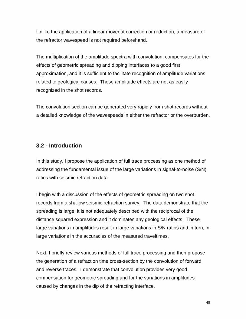
48
Unlike the application of a linear moveout correction or reduction, a measure of
the refractor wavespeed is not required beforehand.
The multiplication of the amplitude spectra with convolution, compensates for the
effects of geometric spreading and dipping interfaces to a good first
approximation, and it is sufficient to facilitate recognition of amplitude variations
related to geological causes. These amplitude effects are not as easily
recognized in the shot records.
The convolution section can be generated very rapidly from shot records without
a detailed knowledge of the wavespeeds in either the refractor or the overburden.
3.2 - Introduction
In this study, I propose the application of full trace processing as one method of
addressing the fundamental issue of the large variations in signal-to-noise (S/N)
ratios with seismic refraction data.
I begin with a discussion of the effects of geometric spreading on two shot
records from a shallow seismic refraction survey. The data demonstrate that the
spreading is large, it is not adequately described with the reciprocal of the
distance squared expression and it dominates any geological effects. These
large variations in amplitudes result in large variations in S/N ratios and in turn, in
large variations in the accuracies of the measured traveltimes.
Next, I briefly review various methods of full trace processing and then propose
the generation of a refraction time cross-section by the convolution of forward
and reverse traces. I demonstrate that convolution provides very good
compensation for geometric spreading and for the variations in amplitudes
caused by changes in the dip of the refracting interface.
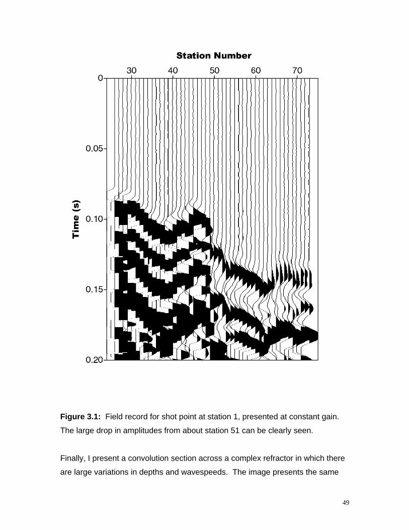
49
Figure 3.1: Field record for shot point at station 1, presented at constant gain.
The large drop in amplitudes from about station 51 can be clearly seen.
Finally, I present a convolution section across a complex refractor in which there
are large variations in depths and wavespeeds. The image presents the same
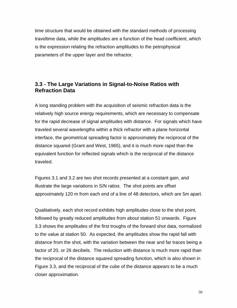
50
time structure that would be obtained with the standard methods of processing
traveltime data, while the amplitudes are a function of the head coefficient, which
is the expression relating the refraction amplitudes to the petrophysical
parameters of the upper layer and the refractor.
3.3 - The Large Variations in Signal-to-Noise Ratios withRefraction Data
A long standing problem with the acquisition of seismic refraction data is the
relatively high source energy requirements, which are necessary to compensate
for the rapid decrease of signal amplitudes with distance. For signals which have
traveled several wavelengths within a thick refractor with a plane horizontal
interface, the geometrical spreading factor is approximately the reciprocal of the
distance squared (Grant and West, 1965), and it is much more rapid than the
equivalent function for reflected signals which is the reciprocal of the distance
traveled.
Figures 3.1 and 3.2 are two shot records presented at a constant gain, and
illustrate the large variations in S/N ratios. The shot points are offset
approximately 120 m from each end of a line of 48 detectors, which are 5m apart.
Qualitatively, each shot record exhibits high amplitudes close to the shot point,
followed by greatly reduced amplitudes from about station 51 onwards. Figure
3.3 shows the amplitudes of the first troughs of the forward shot data, normalized
to the value at station 50. As expected, the amplitudes show the rapid fall with
distance from the shot, with the variation between the near and far traces being a
factor of 20, or 26 decibels. The reduction with distance is much more rapid than
the reciprocal of the distance squared spreading function, which is also shown in
Figure 3.3, and the reciprocal of the cube of the distance appears to be a much
closer approximation.
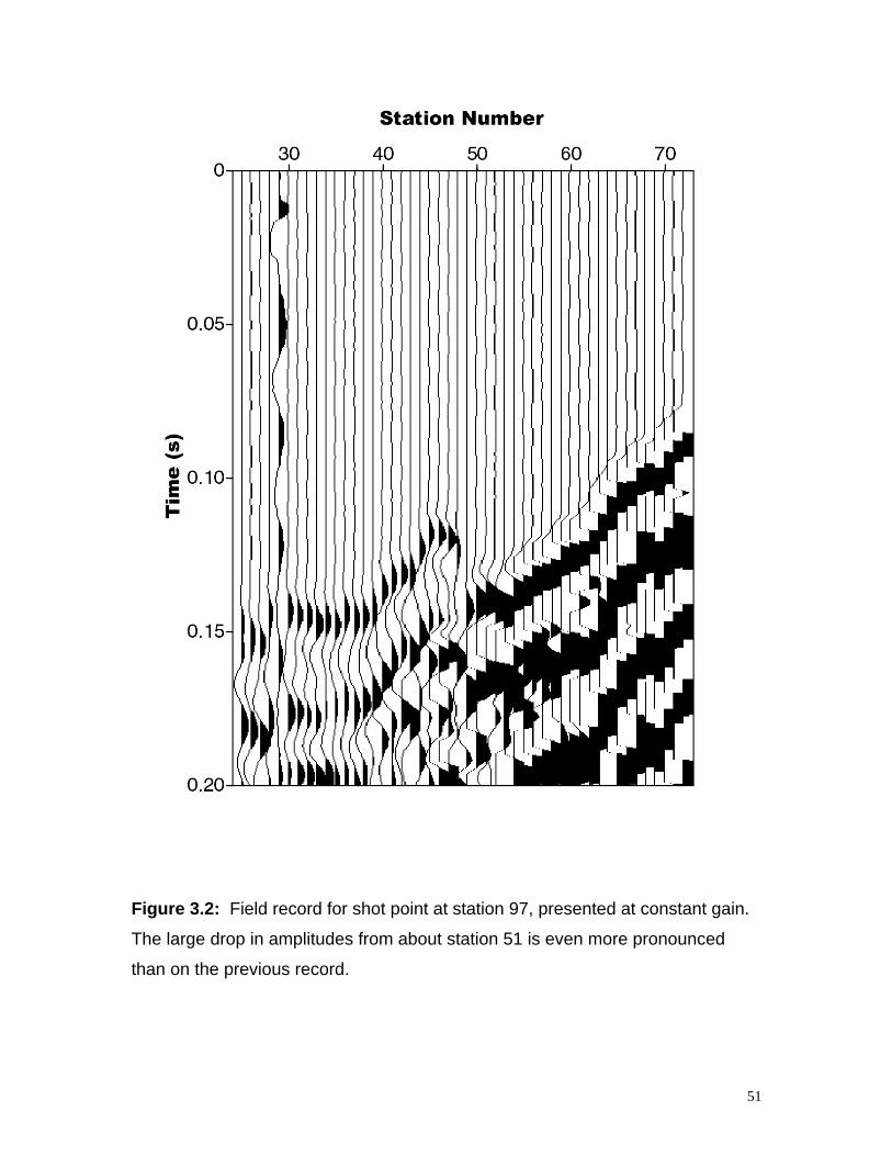
51
Figure 3.2: Field record for shot point at station 97, presented at constant gain.
The large drop in amplitudes from about station 51 is even more pronounced
than on the previous record.
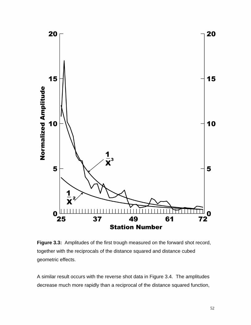
52
Figure 3.3: Amplitudes of the first trough measured on the forward shot record,
together with the reciprocals of the distance squared and distance cubed
geometric effects.
A similar result occurs with the reverse shot data in Figure 3.4. The amplitudes
decrease much more rapidly than a reciprocal of the distance squared function,
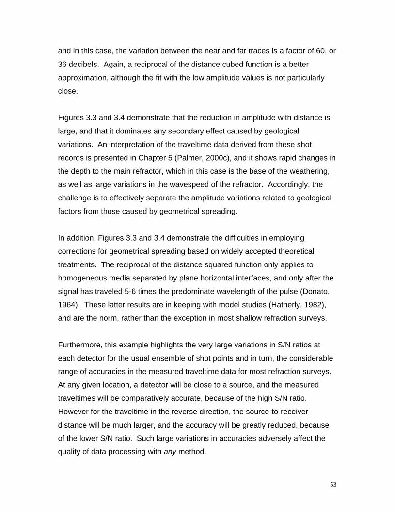
53
and in this case, the variation between the near and far traces is a factor of 60, or
36 decibels. Again, a reciprocal of the distance cubed function is a better
approximation, although the fit with the low amplitude values is not particularly
close.
Figures 3.3 and 3.4 demonstrate that the reduction in amplitude with distance is
large, and that it dominates any secondary effect caused by geological
variations. An interpretation of the traveltime data derived from these shot
records is presented in Chapter 5 (Palmer, 2000c), and it shows rapid changes in
the depth to the main refractor, which in this case is the base of the weathering,
as well as large variations in the wavespeed of the refractor. Accordingly, the
challenge is to effectively separate the amplitude variations related to geological
factors from those caused by geometrical spreading.
In addition, Figures 3.3 and 3.4 demonstrate the difficulties in employing
corrections for geometrical spreading based on widely accepted theoretical
treatments. The reciprocal of the distance squared function only applies to
homogeneous media separated by plane horizontal interfaces, and only after the
signal has traveled 5-6 times the predominate wavelength of the pulse (Donato,
1964). These latter results are in keeping with model studies (Hatherly, 1982),
and are the norm, rather than the exception in most shallow refraction surveys.
Furthermore, this example highlights the very large variations in S/N ratios at
each detector for the usual ensemble of shot points and in turn, the considerable
range of accuracies in the measured traveltime data for most refraction surveys.
At any given location, a detector will be close to a source, and the measured
traveltimes will be comparatively accurate, because of the high S/N ratio.
However for the traveltime in the reverse direction, the source-to-receiver
distance will be much larger, and the accuracy will be greatly reduced, because
of the lower S/N ratio. Such large variations in accuracies adversely affect the
quality of data processing with any method.
54
Figure 3.4: Amplitudes of the first trough measured on the reverse shot record,
together with the reciprocals of the distance squared and distance cubed
geometric effects.
Most methods for the processing of seismic refraction data use simple scalar first
arrival traveltimes, and the problem is normally perceived as achieving
55
satisfactory, rather than uniform S/N ratios. Commonly, a simple gain function is
applied to adjust amplitudes to a convenient level, but this still does not alter the
large variations in S/N ratios. With statics corrections for reflection surveys,
typically a limited source-to-detector interval over which the refraction data are of
sufficient quality, is selected. For geotechnical, groundwater and environmental
studies, the source energy levels are usually increased as far as environmental
and cultural factors permit, or vertical stacking with repetitive sources is
employed.
The following section reviews full trace processing and the issue of the large
variations in S/N ratios.
3.4 - Full Trace Processing Of Refraction Data
Perhaps the simplest approach to full trace processing, is the application of a
linear moveout (LMO) correction to each shot record. With this approach, which
is also known as reduction, each refraction trace is shifted or reduced by a time
equal to the source-to-detector distance, divided by a velocity, which is usually
the known or estimated wavespeed in the target of interest, (Sheriff and Geldart,
1995, Fig. 11.10). The result is normally presented as a set of traces for which
the first arrivals occur at the sum of the source point and detector delay times.
One benefit of this presentation is that it maps any variations in the target depth
in terms of the delay times.
However, this process does not address the basic issue of the large variation in
S/N ratios across the refraction recording spread. The degradation of the arrivals
at the more distant detectors is usually very significant, particularly with crustal
and earthquake studies. Furthermore, it is usually inconvenient to include any
reverse shot records within the same presentation, and therefore to readily
accommodate any lateral variations in wavespeed with irregular refractors.
56
Other approaches are the broadside and fan shooting methods, in which the
source is usually located at an offset point, orthogonal to the center of a linear or
circular array of detectors. Since the source-to-detector distances are essentially
constant, the geometric spreading effects are also constant, and there are much
smaller variations in the S/N ratios from trace to trace. Furthermore, corrections
for the source-to-detector distances, such as with an LMO, in order to emphasize
any structural anomalies in the target refractor, are not essential because such
time shifts are virtually constant also. Examples of the imaging or migration of
broadside data (Mcquillan et al, 1979, Figure 7/15), indicate some of the
possibilities of full trace processing of refraction data.
These methods represent the first true 3D seismic methods for exploration and
pre-date the current reflection 3D methods by many decades (Sheriff and
Geldart, 1995). As such, they will eventually be incorporated into the routine
refraction methods of the future. However, the methods described above do
have two major limitations. They do not determine wavespeeds in the refractor,
nor are they able to separate source and receiver delay times without additional
information, such as borehole control, or the simultaneous recording of a
conventional in-line profile orthogonal to the broadside pattern.
A recent method of imaging refractors with forward and reverse data, is
downward continuation using the tau-p transform (Hill, 1987). It can achieve
good resolution by accommodating diffraction and shadow zone effects. Like all
wavefront methods, it requires an accurate knowledge of the wavespeed of the
upper layer, but this is probably one of the least reliable parameters determined
in most refraction surveys (Chapter 2; Palmer, 1992; Appendix 2).
In this study, I describe the generation of a refraction time section through the
convolution of forward and reverse traces as an effective method of addressing
the fundamental issues of large S/N variations and large moveouts with refraction
57
data. The result, the refraction convolution section (RCS), is similar in
appearance to the familiar reflection time cross section, in which the results are
displayed for example, as a series of wiggle traces.
There are several benefits to processing with this approach. The first is that it is
extremely rapid, avoiding in particular the familiar time consuming tasks of
determining first arrival traveltimes. The second is that little, if any, a priori
information on overburden or refractor wavespeeds is required, although of
course such information is essential for the generation of final depth cross
sections. Accordingly, the convolution section is a very convenient presentation
for an assessment of the quality of processing using other detailed methods,
such as tomography.
In addition, the approximate compensation for large variations in the S/N ratios
facilitates the vertically stacking of refraction data, in a manner analogous to the
common midpoint method with reflection data. This in turn, suggests more
efficient methods of data acquisition with lower environmental impact, particularly
for geotechnical investigations (Palmer, 2000a).
The benefits to interpretation are that the amplitudes obtained through
convolution are essentially a function of the refractor wavespeeds and/or
densities, rather than the source to detector separation. In general, high
wavespeeds and/or densities in the refractor produce low amplitudes. This
relationship between amplitudes and contrasts in the parameters of the refractor
and the overburden provides an additional valuable method for resolving
ambiguities, especially with model-based methods of refraction inversion
(Palmer, 2000c).
The concept of the convolution section was first proposed by Palmer (1976), but
initial tests with Vibroseis data were not especially encouraging, because of
correlation noise before the first breaks (K B S Burke, pers. comm., circa 1982).
58
However, the method was later successfully applied to synthetic data (Taner et
al, 1992).
3.5 - Imaging The Refractor Interface Through The Addition ofForward And Reverse Traveltimes
The unambiguous resolution of dip with plane interfaces or structure with
irregular interfaces, and variable wavespeed within the refractor, usually requires
forward and reverse traveltime data, or off-end data with a high density of source
points, from which the equivalent reversed traveltime data can be generated.
Accordingly, the majority of refraction processing methods explicitly identify and
use forward and reverse traveltimes within their algorithms. These methods
include the wavefront construction methods (Thornburg, 1930; Rockwell, 1967;
Aldridge and Oldenburg, 1992), the conventional reciprocal method (CRM),
(Hawkins, 1961), which is also known as the ABC method in the Americas,
(Nettleton, 1940; Dobrin, 1976), Hagiwara's method in Japan, (Hagiwara and
Omote, 1939), and the plus-minus method in Europe, (Hagedoorn, 1959), Hales'
method, (Hales, 1958; Sjogren, 1979; Sjogren, 1984), and the generalized
reciprocal method (GRM), (Palmer, 1980; Palmer, 1986).
There are minor differences in detail between the algorithms for each of these
methods. These differences include whether the reciprocal time, the time from
the forward shot point to the reverse shot point, is used, the inclusion of the
factor of a half, or whether the offset distance, which is the horizontal separation
between the point of refraction on the interface and the detector position on the
surface, is accommodated through the operation known as refraction migration
(Palmer, 1986, p.74-80).
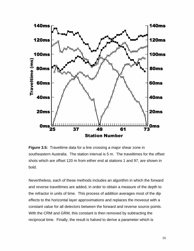
59
Figure 3.5: Traveltime data for a line crossing a major shear zone in
southeastern Australia. The station interval is 5 m. The traveltimes for the offset
shots which are offset 120 m from either end at stations 1 and 97, are shown in
bold.
Nevertheless, each of these methods includes an algorithm in which the forward
and reverse traveltimes are added, in order to obtain a measure of the depth to
the refractor in units of time. This process of addition averages most of the dip
effects to the horizontal layer approximations and replaces the moveout with a
constant value for all detectors between the forward and reverse source points.
With the CRM and GRM, this constant is then removed by subtracting the
reciprocal time. Finally, the result is halved to derive a parameter which is
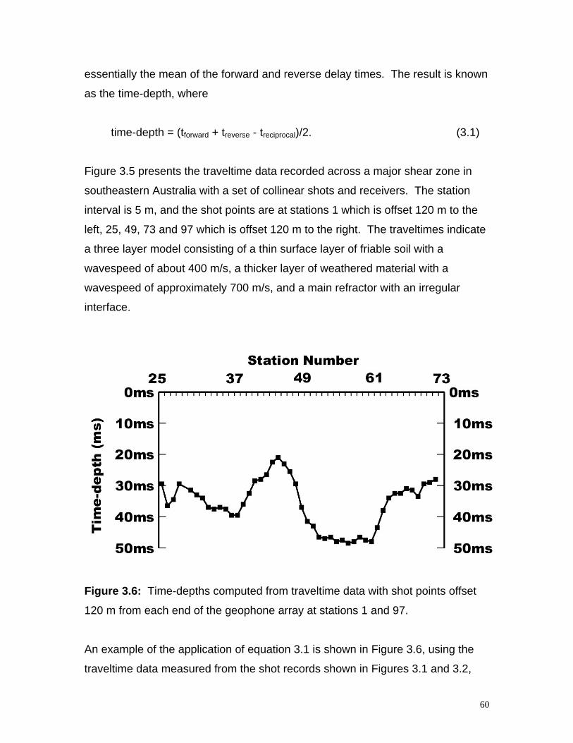
60
essentially the mean of the forward and reverse delay times. The result is known
as the time-depth, where
time-depth = (tforward + treverse - treciprocal)/2. (3.1)
Figure 3.5 presents the traveltime data recorded across a major shear zone in
southeastern Australia with a set of collinear shots and receivers. The station
interval is 5 m, and the shot points are at stations 1 which is offset 120 m to the
left, 25, 49, 73 and 97 which is offset 120 m to the right. The traveltimes indicate
a three layer model consisting of a thin surface layer of friable soil with a
wavespeed of about 400 m/s, a thicker layer of weathered material with a
wavespeed of approximately 700 m/s, and a main refractor with an irregular
interface.
Figure 3.6: Time-depths computed from traveltime data with shot points offset
120 m from each end of the geophone array at stations 1 and 97.
An example of the application of equation 3.1 is shown in Figure 3.6, using the
traveltime data measured from the shot records shown in Figures 3.1 and 3.2,
61
and summarized in bold in Figure 3.5. The time-depths have been computed
with a reciprocal time of 147 ms, (Palmer, 1980, equation 33), and an optimum
XY value of 5 meters.
The XY value is the separation between the pairs of forward and reverse
traveltimes used in equation 3.1, and it is usually a multiple of the detector
spacing. The optimum XY value is obtained with the minimum variance criterion
described elsewhere (Palmer, 1980, p.31-35) and it is the sum of the forward and
reverse offset distances. This sum is essentially independent of the dip angles,
unlike the individual forward and reverse components. At the optimum XY value,
the forward and reverse rays are refracted from near the same point on the
refractor and the smoothing effects of other XY values are minimized.
3.6 - The Addition of Traveltimes With Convolution
The traditional methods for the inversion of refraction data, can be categorized by
how the addition of the forward and reverse traveltimes is implemented. The
wavefront construction and Hales' methods achieve it graphically, while the CRM
and GRM achieve it with the simple addition of two numbers.
In this study, I demonstrate the use of convolution of forward and reverse traces
to effectively achieve the addition.
The convolution process has usually been associated with filtering. Its effect can
be described in the frequency domain, as the multiplication of the amplitude
spectra and the addition of the phase spectra of the two functions.
A similar result occurs with the convolution of two seismic refraction traces. The
amplitude spectra are multiplied, and the arrival times, which are contained within
the phase spectra, are added.
62
Alternatively, the addition of first arrival times with convolution can be
demonstrated with the z transform notation (Sheriff and Geldart, 1995). The
digitized seismic trace can be represented as a polynomial in z, in which the
exponent represents the sample number. The forward trace F(z) is given by
F(z) = fm zm + fm+1 zm+1 + fm+2 zm+2 + .... (3.2)
where fj = 0 for j < m.
The forward traveltime is m, since fm is the first non-zero amplitude for the
forward trace and therefore represents the onset of seismic energy. Similarly,
the reverse trace R(z) is given by
R(z) = rn zn + rn+1 zn+1 + rn+2 zn+2 + .... (3.3)
where rj =0 for j < n. In this case, the reverse traveltime is n, since rn is the first
non-zero amplitude.
Convolution in the z domain is achieved by polynomial multiplication, ie.
F(z) * R(z) = fm rn zm + n + (fm rn+1 + fm+1 rn) zm + n + 1
+ (fm rn+2+ fm+1 rn+1 + fm+2 rn) zm+n+2 + .... (3.4)
It can be seen that the first non-zero coefficient is fm rn and it occurs at the time m
+ n, which is at the sum of the forward and reverse traveltimes.
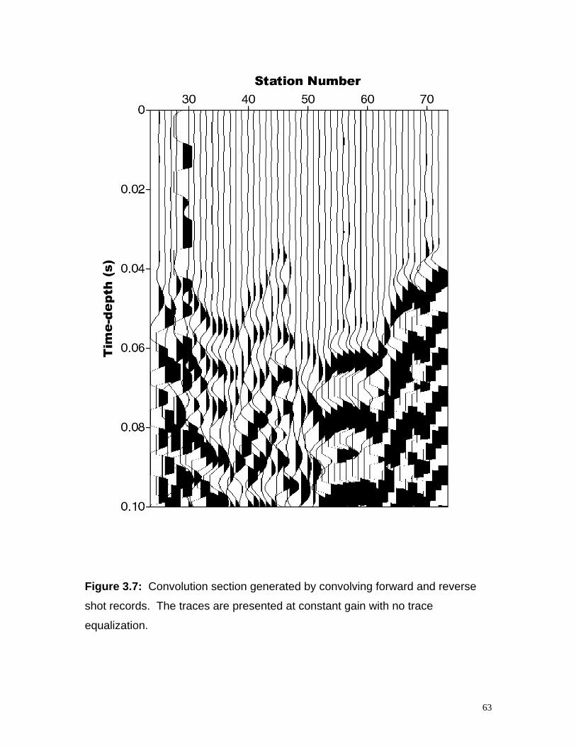
63
Figure 3.7: Convolution section generated by convolving forward and reverse
shot records. The traces are presented at constant gain with no trace
equalization.
64
The convolution section generated with the shot records in Figures 3.1 and 3.2
and an XY separation of 5 m, is shown in Figure 3.7. Each trace in fact
represents the time-depth, as both the subtraction of the reciprocal time and the
halving of the time scale have been carried out. (These operations were readily
achieved with software for processing seismic reflection data, by treating the
reciprocal time as a static correction and by halving the sampling interval in the
trace headers.)
It is immediately apparent that the moveout has been removed by the
convolution process. The convolution section shows the same structure on the
refractor interface as that obtained in Figure 3.6 with the traveltime data.
In addition, perhaps the other striking effect of the convolution section is the
convenient presentation of the amplitude information. It is clear that convolution
has compensated for the very large amplitude variations related to geometrical
spreading and other factors with the shot records, and that the signal-to-noise
ratios of the convolved traces are very similar. Although the compensation is not
exact, as will be shown below, it is still sufficient to permit the recognition of
amplitude variations related to geological factors.
However, the interface computed using traveltimes in Figure 3.6 is about 10 ms
shallower than that recognizable from the convolution section in Figure 3.7. This
discrepancy arises from the various gain functions used with each approach.
The time-depths in Figure 3.6 were computed with traveltimes at which the first
onset of seismic energy was detected on the shot records, using as high a gain
as was possible without the background noise causing any detectable deflections
before the first breaks. This gain is usually sufficient to cause clipping of most of
the seismic data after the first arrivals. On the other hand, the presentation gain
in Figure 3.7 is much lower, and it has been selected to permit the examination of
the first few cycles after the computed time-depth.
65
3.7 - The Effects of Geometrical Spreading on the ConvolutionSection Amplitudes
The shot record amplitudes shown in Figures 3.3 and 3.4 demonstrate the very
large variations due to geometrical spreading, as well as the difficulties in
selecting an appropriate mathematical description. Figure 3.8 shows normalized
theoretical amplitudes for reciprocal distance squared and reciprocal distance
cubed functions for a shot at station 1. The values are normalized to that at
station 72, which is the most distant detector from the shot at station 1. The
variation in amplitude between the first and last detectors is about 19 db for
reciprocal distance squared spreading, while it is 28.6 db for the reciprocal
distance cubed case, with an average of about 24 db.
Figure 3.8 also shows the geometrical effects for the convolved traces, obtained
with equation 3.5, viz.
Geometric factor convolved trace = 1 / (Xn (L-X)n) (3.5)
where, X is the distance from one shot point to the detector, L is the shot point to
shot point distance, which in this case is 480 m, and n is 2 for the reciprocal
distance squared and 3 for the reciprocal distance cubed cases. The convolved
amplitudes have been normalized to the minimum values which are at station 49,
the midpoint of the shot point to shot point distance. The maximum variation in
the convolved amplitudes is between the ends and the midpoint of the detector
array, and is 5 db for n equal to 2 and 7.5 db for n equal to 3, with an average of
about 6 db.
It is clear that convolution has reduced the effects of geometrical spreading by
approximately 18 db, but that a residual geometric effect of about 6 db still
remains. However, the reduction is sufficient to be able to recognize amplitude
variations related to geological effects. This is shown in Figure 3.9, with the
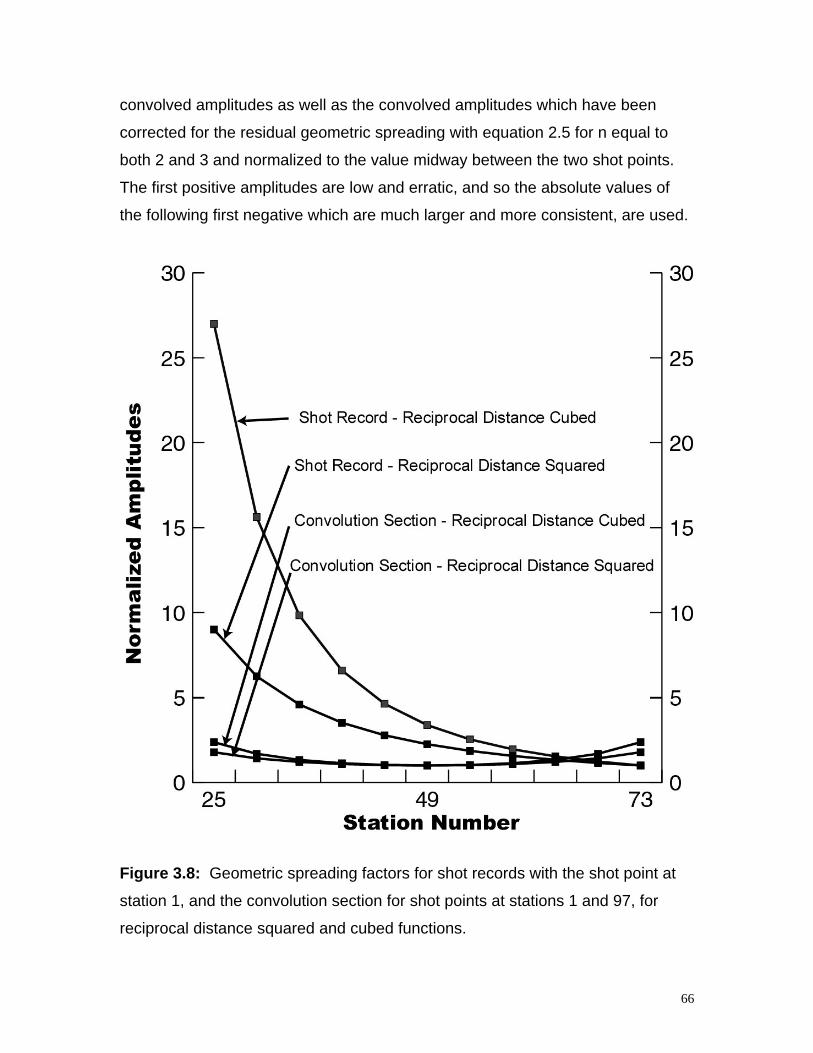
66
convolved amplitudes as well as the convolved amplitudes which have been
corrected for the residual geometric spreading with equation 2.5 for n equal to
both 2 and 3 and normalized to the value midway between the two shot points.
The first positive amplitudes are low and erratic, and so the absolute values of
the following first negative which are much larger and more consistent, are used.
Figure 3.8: Geometric spreading factors for shot records with the shot point at
station 1, and the convolution section for shot points at stations 1 and 97, for
reciprocal distance squared and cubed functions.
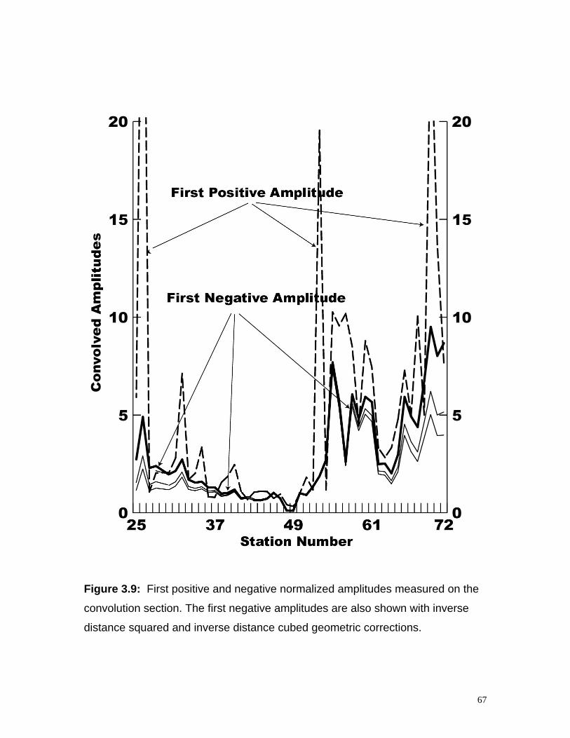
67
Figure 3.9: First positive and negative normalized amplitudes measured on the
convolution section. The first negative amplitudes are also shown with inverse
distance squared and inverse distance cubed geometric corrections.
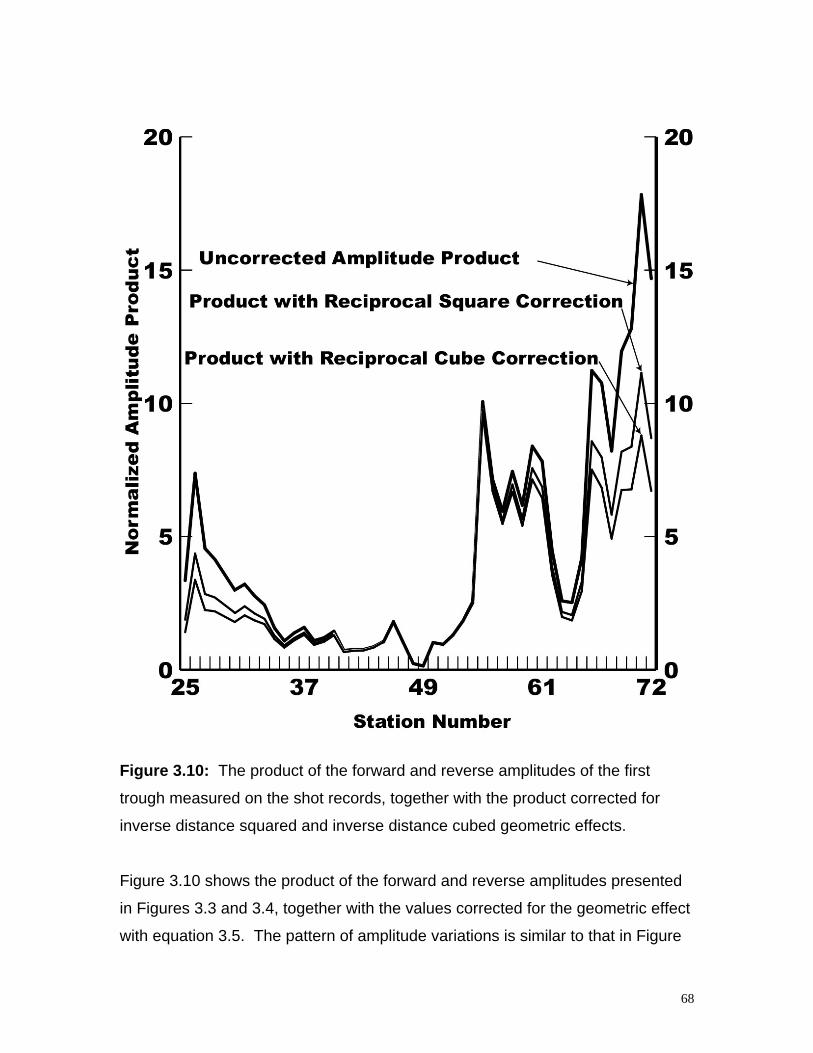
68
Figure 3.10: The product of the forward and reverse amplitudes of the first
trough measured on the shot records, together with the product corrected for
inverse distance squared and inverse distance cubed geometric effects.
Figure 3.10 shows the product of the forward and reverse amplitudes presented
in Figures 3.3 and 3.4, together with the values corrected for the geometric effect
with equation 3.5. The pattern of amplitude variations is similar to that in Figure
69
3.9, confirming that convolution has in fact multiplied the amplitudes, and that the
product has greatly reduced the geometrical effect.
In both Figures 3.9 and 3.10, it is possible to separate the convolved and
multiplied amplitudes into four regions which correlate well with those recognized
in chapter 5, (Palmer, 2001), using wavespeed and depth. Correction of the
convolved and multiplied amplitude products with the theoretical geometrical
effects improves the ease in recognizing the four regions, but does not alter the
general features of the amplitudes.
3.8 - Effects Of Refractor Dip On Convolution Amplitudes
The convolution of forward and reverse traces provides an approximate
correction for the effects of a dipping interface on the amplitudes measured with
vertical component geophones. Suppose the angle from the vertical at which a
critically refracted ray approaches the surface is α for a horizontal refractor. The
vertical component measured with the standard geophone will be the forward or
reverse amplitude multiplied by cosα. Therefore, the convolved amplitude will be
multiplied by cos2α, ie.
Convolved Amphorizontal refractor = cos2α Ampforward Ampreverse (3.6)
Next, suppose the refractor has a dip of θ. The vertical component measured will
be the shot amplitude multiplied by cos(α+θ) in one direction, cos(α-θ) in the
reverse direction.
Vertical Shot Amp dipping refractor = cos(α±θ) Amp (3.7)
The vertical component of the convolved amplitude is given by equation 3.8, viz.
70
Convolved Ampdipping refractor =(cos2α cos2θ - sin2α sin2θ) Ampforward Ampreverse
(3.8)
For small dip angles, say less than about fifteen degrees, the second order terms
in sinθ can be neglected, while the cos2θ term is approximately one. Therefore,
to sufficient accuracy the product of the forward and reverse amplitudes achieved
with convolution is given by
Convolved Ampdipping refractor = cos2α Ampforward Ampreverse (3.9)
Accordingly, amplitudes computed for plane horizontal refractors (Heelan, 1953;
Werth, 1967) can still be usefully applied to dipping layers when convolution is
employed.
3.9 - Conclusions
Seismic refraction acquisition techniques are characterised by large source to
receiver distances. Commonly, these distances are greater than about four
times the depth of the target, whereas for reflection methods, the equivalent
distances are less than the target depth. The large distances produce
commensurately large moveouts between adjacent traces and large amplitude
variations between the near and far traces.
The wide range of refraction amplitudes is the result of the rapid geometric
spreading factor, which is at least the reciprocal of the distance squared, and it
produces considerable variation in S/N ratios. Accordingly, most refraction
inversion methods use traveltime data with widely varying accuracies, which are
related to the large variations in signal-to-noise ratios.
71
The time section, generated by convolving forward and reverse seismic traces
together with a static shift equal to the reciprocal time, addresses both issues of
large moveouts between adjacent traces and large amplitude variations.
The addition of the phase spectra with convolution effectively adds the forward
and reverse traveltimes. This process of addition is common to most of the
standard techniques for the inversion of refraction data. The convolution section
after shifting by the reciprocal time, shows the same structural features of the
refractor in units of time, as is obtained with the standard approaches.
Furthermore, the convolution section can be generated without a prior knowledge
of the wavespeeds in either the upper layer, as is required with the downward
continuation methods, or in the refractor, as is required with the application of a
linear moveout correction or reduction. This latter is especially important where
there are significant lateral variations in the wavespeed of the refractor.
The multiplication of the amplitude spectra with convolution, to a good first
approximation, effectively compensates for the effects of geometric spreading,
which can be significantly larger than the commonly assumed reciprocal of the
distance squared function. This compensation is generally sufficient to be able to
recognize amplitude variations related to geological causes, which are not as
easily detected in the shot records. The correlation of any amplitude variations
with the structural variations on the interface of the refractor can be more
conveniently and more rapidly carried out using the convolution section, than for
example by multiplying amplitudes measured on the shot records.
If necessary, a geometric correction based on the product of a reciprocal of the
distance power function in the forward and reverse directions, can be applied to
the convolution section. This correction exhibits a much reduced variation
72
compared with those for the individual shot records, and it is most useful near the
shot points where it can have a value of up to a factor of about 2, or 6 decibels.
The ease and convenience of generating the convolution section facilitate its
inclusion in the routine processing of seismic refraction data using any method.
3.10 - References
Aldridge, D. F., and Oldenburg, D. W., 1992, Refractor imaging using an
automated wavefront reconstruction method: Geophysics, 57, 378-385.
Dobrin, M. B., 1976, Introduction to geophysical prospecting, 3rd edition:
McGraw-Hill Inc.
Donato, R. J., 1964, Amplitude of P head waves: J. Acoust. Soc. Am., 36, 19-25.
Grant, F. S., and West, G. F., 1965, Interpretation theory in applied geophysics:
McGraw-Hill Inc.
Hagedoorn, J. G., 1959, The plus-minus method of interpreting seismic refraction
sections: Geophys. Prosp, 7, 158-182.
Hagiwara, T., and Omote, S., 1939, Land creep at Mt Tyausa-Yama
(Determination of slip plane by seismic prospecting): Tokyo Univ. Earthquake
Res. Inst. Bull., 17, 118-137.
Hales, F. W., 1958, An accurate graphical method for interpreting seismic
refraction lines: Geophys. Prosp., 6, 285-294.
73
Hatherly, P. J., 1982, Wave equation modelling for the shallow seismic refraction
method: Expl. Geophys., 13, 26-34.
Hawkins, L. V., 1961, The reciprocal method of routine shallow seismic refraction
investigations: Geophysics, 26, 806-819.
Heelan, P. A., 1953, On the theory of head waves: Geophysics, 18, 871-893.
Hill, N. R., 1987, Downward continuation of refracted arrivals to determine
shallow structure: Geophysics, 52, 1188-1198.
McQuillan, R., Bacon, M., and Barclay, W., 1979, An introduction to seismic
interpretation: Graham & Trotman Limited.
Nettleton, L. L., 1940, Geophysical prospecting for oil: McGraw-Hill Book
Company Inc.
Palmer, D., 1976, An application of the time section in shallow seismic
refraction studies: Master's thesis, The University of Sydney.
Palmer, D., 1980, The generalized reciprocal method of seismic refraction
interpretation: Society of Exploration Geophysicists.
Palmer, D., 1986, Refraction seismics: the lateral resolution of structure and
seismic velocity: Geophysical Press.
Palmer, D., 1992, Is forward modeling as efficacious as minimum variance for
refraction inversion?: Explor. Geophys. 23, 261-266, 521.
Palmer, D., 2000a, Can new acquisition methods improve signal-to-noise ratios
with seismic refraction techniques?: Explor. Geophys., 31, 275-300.
74
Palmer, D., 2000b, Can amplitudes resolve ambiguities in refraction inversion?:
Explor. Geophys., 31, 304-309.
Palmer, D., 2001, Resolving Refractor Ambiguities With Amplitudes: Geophysics
66, 1590-1593.
Rockwell, D. W., 1967, A general wavefront method, in Musgrave, A .W., Ed.,
Seismic Refraction Prospecting: Society of Exploration Geophysicists, 363-415.
Sheriff, R. E., and Geldart, L. P., 1995, Exploration Seismology, 2nd edition:
Cambridge University Press.
Sjogren, B., 1979, Refractor velocity determination - cause and nature of some
errors: Geophys. Prosp., 27, 507-538.
Sjogren, B., 1984, Shallow refraction seismics: Chapman and Hall.
Taner, M. T., Matsuoka, M., Baysal, E., Lu, L., and Yilmaz, O., 1992, Imaging
with refractive waves: 62nd Ann. Internat. Mtg., Soc. Expl. Geophys.
Thornburg, H. R., 1930, Wavefront diagrams in seismic interpretation: AAPG
Bulletin, 14, 185-200.
Werth, G. A., 1967, Method for calculating the amplitude of the refraction arrival,
in Musgrave, A. W., Ed., Seismic refraction prospecting: Society of Exploration
Geophysicists, 119-137.
75
Chapter 4
Starting Models For RefractionInversion
4.1 - Summary
The algorithms of the generalized reciprocal method (GRM) are applied to a set
of reversed traveltime data for a two layer model with a synclinal refractor
interface, in order to generate a family of starting models. Each starting model
shows much the same depths as the original model, but each has a narrow zone
in the refractor with an anomalous wavespeed. The traveltimes through each of
the starting models differ from those for the original model by less than a
millisecond. If any were used as starting models for tomographic or model-based
inversion, then the final result would show only minor differences. This example
demonstrates the non-uniqueness of model-based inversion.
In order to address the issues of non-uniqueness with model-based inversion, it
is recommended that a range of starting models, such as those which can be
generated with the GRM, be used.
Alternatively, other approaches, which aim to resolve these ambiguities, can be
employed. In many cases, the minimum variance criterion of the GRM can
resolve whether lateral variations in the refractor wavespeeds are genuine, or
whether they are artifacts of the inversion algorithm. In addition, it is proposed
76
that the amplitudes of the refraction convolution section can indicate where there
are genuine changes in the wavespeed of the refractor, because the amplitudes
are a function of the contrasts in wavespeeds between the refractor and the layer
above.
4.2 - Introduction
The inversion of seismic refraction data with model-based or tomographic
methods consists of deriving a starting model of the subsurface with standard
algorithms, and then testing it by comparing the computed traveltimes of the
model with the observed data. If there are differences, then the model is
adjusted until an acceptable agreement is achieved. Commonly, several
iterations may be required.
While most geophysicists are satisfied to generate a model which reproduces the
observations, there is the fundamental theoretical reality that an infinite number
of solutions can reproduce the data (Oldenburg, 1984; Treitel and Lines, 1988),
although not all of these solutions will be geologically plausible. This non-
uniqueness becomes more significant where the data are inaccurate and
incomplete as is often the case with field data, and where models, which do not
fit the data precisely, are accepted.
The issues of non-uniqueness are not usually considered with shallow refraction
tomography. The non-uniqueness includes the wavespeeds in both the
overburden and the refractor and they are often inter-related. One compelling
example is the somewhat paradoxical situation of the poor determination of
wavespeeds in the refractor, despite the fact that over 90% of traveltimes are
from that layer (Lanz et al, 1998, Figure 8). This situation is at variance with the
experiences of most seismologists using more traditional methods of refraction
77
processing, and it is probably related to the use of a linear wavespeed function
with a very high gradient in the upper layer.
Previous studies (Hagedoorn, 1955) have demonstrated the ambiguities in
determining the wavespeed stratification within a single layer above the refractor.
Even in the absence of undetected layers, generally known as hidden layers
within the blind zone and reversals in wavespeed, it is not possible to accurately
specify the mathematical function which describes the wavespeed in the
overlying layer. As a result, there is a large range in the depths to the refractor
computed with the various mathematical functions which can be fitted to the first
arrival traveltime data with acceptable accuracy.
Palmer (1992, Appendix 2) has demonstrated, that when the refractor interface is
sufficiently irregular in relation to its depth, the generalized reciprocal method
(GRM) (Palmer, 1980; 1986), can significantly improve the accuracy of the depth
computations for a wide range of mathematical functions in the upper layer. The
mathematical functions include wavespeed reversals and transverse isotropy,
which are not adequately addressed with other approaches.
This study examines the non-uniqueness in the determination of the wavespeeds
in the refractor. In these cases, the non-uniqueness is usually related to the
starting model for the inversion process and in turn, to the selection of the
inversion algorithm used to generate that model.
I demonstrate that a range of geologically plausible starting models can be
readily generated from the one set of reversed traveltime data with the algorithms
of the GRM, and that each of these models fits the data to an acceptable
accuracy of a few milliseconds. I conclude that the selection of the initial starting
model is critical with model-based methods of refraction inversion. I further
conclude that the issues of non-uniqueness, which currently are not adequately
examined with most model-based methods for inverting refracting data, can be
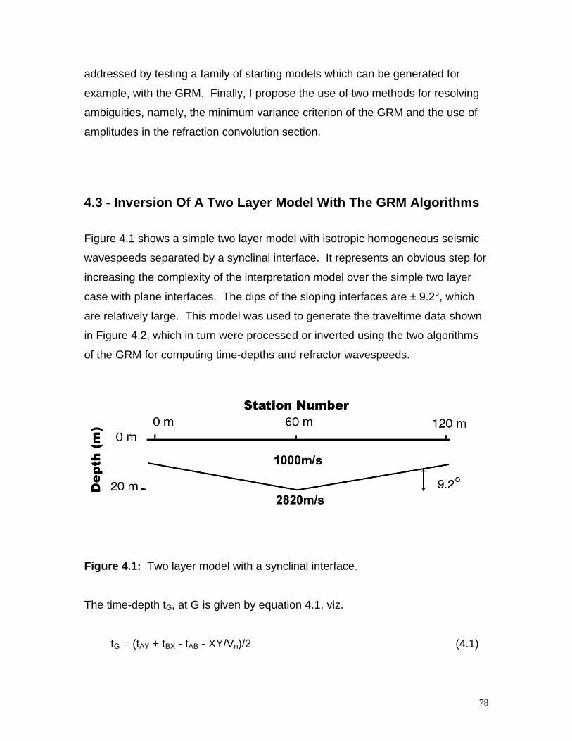
78
addressed by testing a family of starting models which can be generated for
example, with the GRM. Finally, I propose the use of two methods for resolving
ambiguities, namely, the minimum variance criterion of the GRM and the use of
amplitudes in the refraction convolution section.
4.3 - Inversion Of A Two Layer Model With The GRM Algorithms
Figure 4.1 shows a simple two layer model with isotropic homogeneous seismic
wavespeeds separated by a synclinal interface. It represents an obvious step for
increasing the complexity of the interpretation model over the simple two layer
case with plane interfaces. The dips of the sloping interfaces are ± 9.2°, which
are relatively large. This model was used to generate the traveltime data shown
in Figure 4.2, which in turn were processed or inverted using the two algorithms
of the GRM for computing time-depths and refractor wavespeeds.
Figure 4.1: Two layer model with a synclinal interface.
The time-depth tG, at G is given by equation 4.1, viz.
tG = (tAY + tBX - tAB - XY/Vn)/2 (4.1)
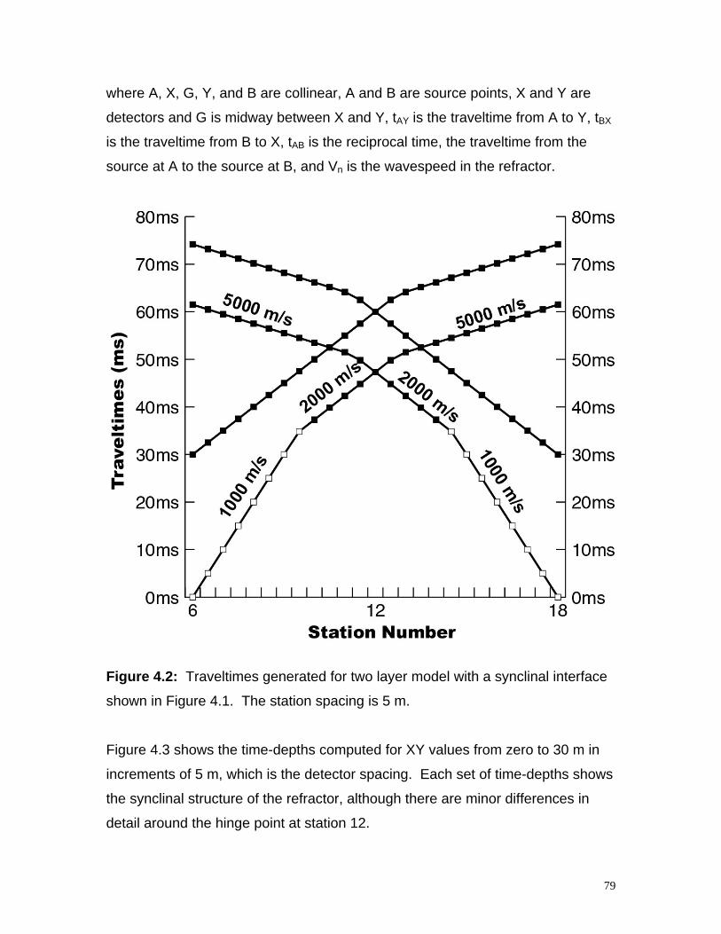
79
where A, X, G, Y, and B are collinear, A and B are source points, X and Y are
detectors and G is midway between X and Y, tAY is the traveltime from A to Y, tBX
is the traveltime from B to X, tAB is the reciprocal time, the traveltime from the
source at A to the source at B, and Vn is the wavespeed in the refractor.
Figure 4.2: Traveltimes generated for two layer model with a synclinal interface
shown in Figure 4.1. The station spacing is 5 m.
Figure 4.3 shows the time-depths computed for XY values from zero to 30 m in
increments of 5 m, which is the detector spacing. Each set of time-depths shows
the synclinal structure of the refractor, although there are minor differences in
detail around the hinge point at station 12.
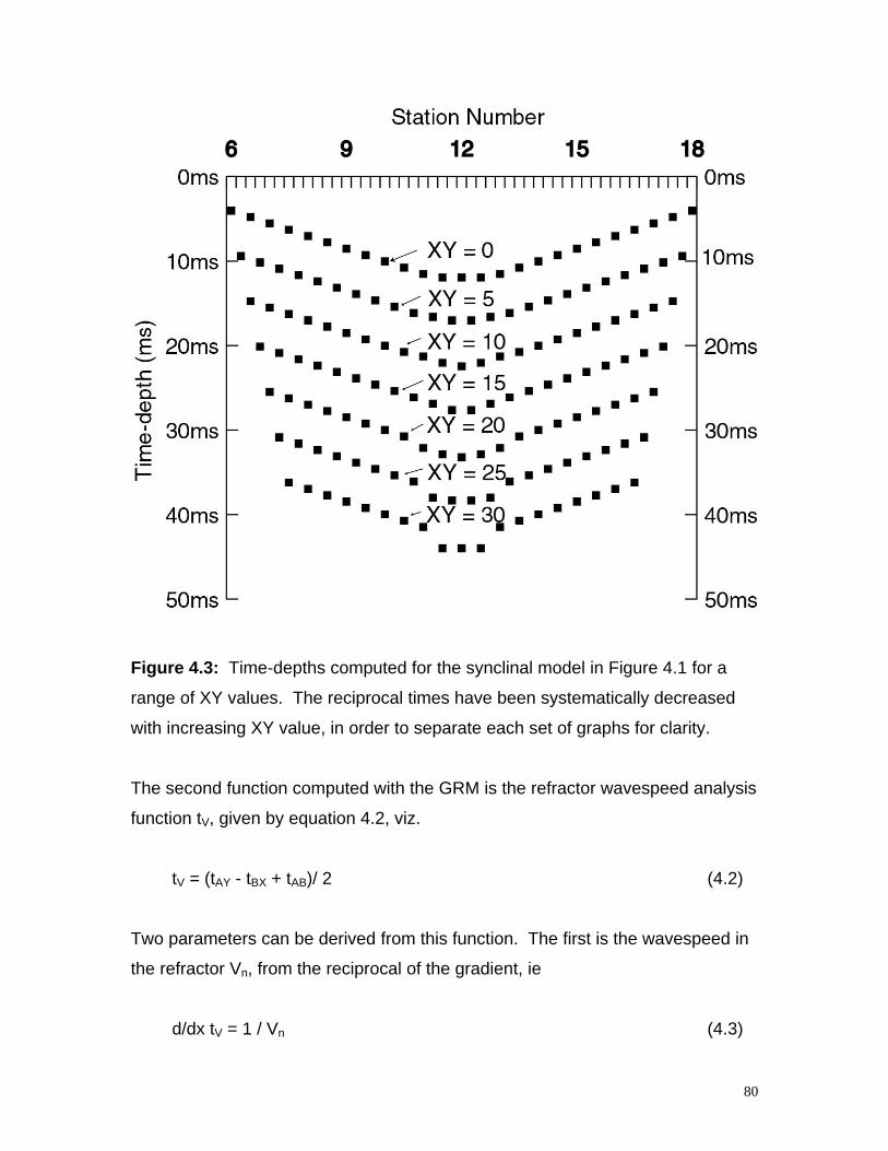
80
Figure 4.3: Time-depths computed for the synclinal model in Figure 4.1 for a
range of XY values. The reciprocal times have been systematically decreased
with increasing XY value, in order to separate each set of graphs for clarity.
The second function computed with the GRM is the refractor wavespeed analysis
function tV, given by equation 4.2, viz.
tV = (tAY - tBX + tAB)/ 2 (4.2)
Two parameters can be derived from this function. The first is the wavespeed in
the refractor Vn, from the reciprocal of the gradient, ie
d/dx tV = 1 / Vn (4.3)
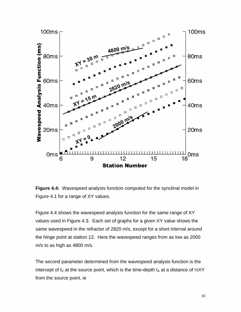
81
Figure 4.4: Wavespeed analysis function computed for the synclinal model in
Figure 4.1 for a range of XY values.
Figure 4.4 shows the wavespeed analysis function for the same range of XY
values used in Figure 4.3. Each set of graphs for a given XY value shows the
same wavespeed in the refractor of 2820 m/s, except for a short interval around
the hinge point at station 12. Here the wavespeed ranges from as low as 2000
m/s to as high as 4800 m/s.
The second parameter determined from the wavespeed analysis function is the
intercept of tV at the source point, which is the time-depth tA at a distance of ½XY
from the source point, ie
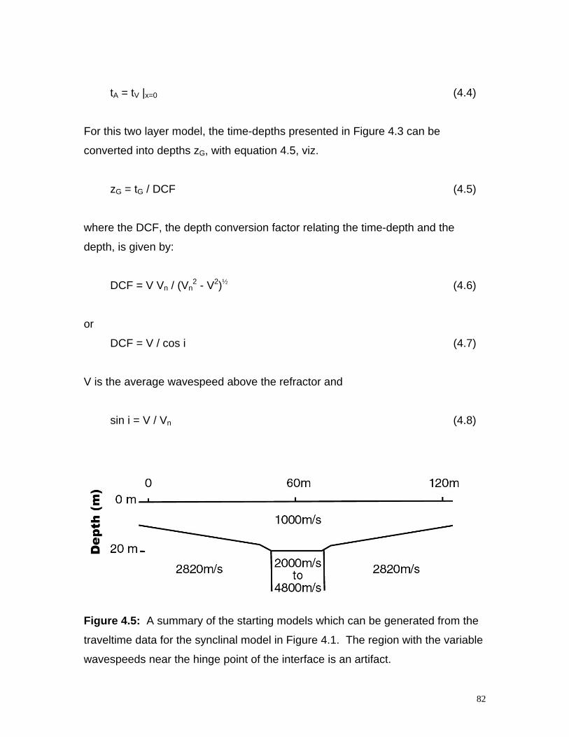
82
tA = tV |x=0 (4.4)
For this two layer model, the time-depths presented in Figure 4.3 can be
converted into depths zG, with equation 4.5, viz.
zG = tG / DCF (4.5)
where the DCF, the depth conversion factor relating the time-depth and the
depth, is given by:
DCF = V Vn / (Vn2 - V2)½ (4.6)
or
DCF = V / cos i (4.7)
V is the average wavespeed above the refractor and
sin i = V / Vn (4.8)
Figure 4.5: A summary of the starting models which can be generated from the
traveltime data for the synclinal model in Figure 4.1. The region with the variable
wavespeeds near the hinge point of the interface is an artifact.
83
Figure 4.5 is a summary of the range of depth models which can be generated
with the XY values from zero to 30 m. Although the depth sections reproduce the
synclinal structure of the original model, there is an additional segment in the
second layer with wavespeeds from 2000 m/s to 4800 m/s which is not present in
the original model. This additional segment could represent a weathered dyke or
a shear zone for the low wavespeed cases or an unweathered dyke or a silicified
shear zone for the high wavespeed cases. Therefore, all models are geologically
both plausible and significant. Nevertheless, they are artifacts generated by
equation 4.2, the refractor wavespeed analysis algorithm.
4.4 - Time Differences Between Starting Models
Figure 4.6 shows the time-depths for the range of XY values from zero to 30 m
plotted without the vertical separation obtained by changing the reciprocal time
tAB, in equation 4.1. This presentation, which emphasizes the subtle variations
between different XY values, shows that the time-depth values are identical for
the planar sloping surfaces, but diverge by less than 2 ms in the vicinity of the
hinge point.
The smaller values are associated with the XY values which are less than the
optimum of 15 m and in turn are associated with the zone of lower wavespeeds
in the refractor. Although there is a slightly higher DCF computed with equation
4.6 in this narrow region, there is still a reduction in depth at the hinge point, and
in turn a small decrease in traveltimes in the upper layer. This decrease
approximately compensates for the slight increase in traveltimes in the region of
lower wavespeeds in the refractor.
The larger time-depth values are associated with the XY values which are
greater than the optimum of 15 m and in turn are associated with the zone of
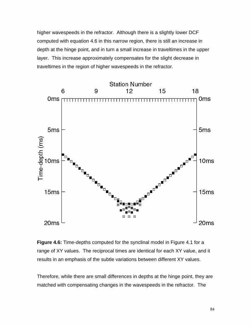
84
higher wavespeeds in the refractor. Although there is a slightly lower DCF
computed with equation 4.6 in this narrow region, there is still an increase in
depth at the hinge point, and in turn a small increase in traveltimes in the upper
layer. This increase approximately compensates for the slight decrease in
traveltimes in the region of higher wavespeeds in the refractor.
Figure 4.6: Time-depths computed for the synclinal model in Figure 4.1 for a
range of XY values. The reciprocal times are identical for each XY value, and it
results in an emphasis of the subtle variations between different XY values.
Therefore, while there are small differences in depths at the hinge point, they are
matched with compensating changes in the wavespeeds in the refractor. The
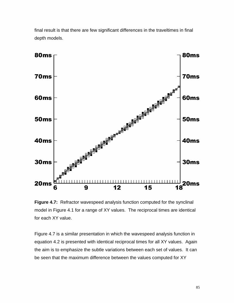
85
final result is that there are few significant differences in the traveltimes in final
depth models.
Figure 4.7: Refractor wavespeed analysis function computed for the synclinal
model in Figure 4.1 for a range of XY values. The reciprocal times are identical
for each XY value.
Figure 4.7 is a similar presentation in which the wavespeed analysis function in
equation 4.2 is presented with identical reciprocal times for all XY values. Again
the aim is to emphasize the subtle variations between each set of values. It can
be seen that the maximum difference between the values computed for XY
86
values of zero and 30 m is 2.2 ms and that maximum difference between the any
set and those computed with optimum XY value of 15 m is less than 1.1 ms.
Figure 4.7 also demonstrates a fundamental problem in determining wavespeeds
in narrow intervals of the refractor with seismic refraction methods. The variation
in wavespeed in the refractor of 2000 m/s to 4800 m/s is very large and
geologically significant. However, these variations in wavespeed do not result in
commensurately large changes in traveltimes. An inspection of Figure 4.4 shows
that a single wavespeed can be fitted to each set of points with an accuracy of
better than a millisecond.
The significance of Figures 4.6 and 4.7 is that the time differences between each
model of the refractor computed with the selected range of XY values are subtle
and are generally within 1 ms of that computed with the optimum XY value of 15
m. These differences are typical of the acceptable residuals for most model-
based or tomographic methods of inversion.
4.5 - Agreement Between Starting Models And Traveltime Data
The small time differences between the various models as shown in Figures 4.6
and 4.7 suggest that each model should closely honor the original traveltime
data. Such a result is in fact the norm with the GRM, because the algorithms
seek to separate or analyze the traveltimes into the source point and detector
time-depths, together with the traveltime in the refractor, while still preserving the
original traveltime data. This is demonstrated by the simple addition of equations
4.1 and 4.2, viz.
tAY = tG + tV + ½ XY/Vn (4.9)
From equations 4.3 and 4.4, it is readily shown that
87
tV = tA + AG/Vn (4.10)
Equations 4.9 and 4.10 can be combined to obtain
tAY = tG + tA + AY / Vn (4.11)
4.6 - Discussion
This study illustrates some of the inherent problems of non-uniqueness with
determining wavespeeds in the refractor. Using a simple model and the GRM
algorithms, it is possible to generate a family of starting models, each of which
has much the same depths to the refractor as the original model but each of
which includes a narrow zone in the refractor with an anomalous wavespeed.
Even with the noise-free model data used in this study, the time differences are
generally less than one millisecond, which is the error commonly assigned to the
measurement of traveltimes from field data, and which is within the range of
acceptable residuals for tomography. Therefore, if any were used as starting
models for tomography, then there would be minimal differences with the final
result of the inversion process. Furthermore, all of these models are geologically
meaningful and hence cannot be readily discarded.
(As an aside, geologically meaningless models can also be generated with the
GRM, simply by increasing the XY value in the wavespeed analysis function in
equation 4.2, until negative wavespeeds are obtained with equation 4.3.)
Frequently, the algorithms of the standard reciprocal method (SRM) (Hawkins,
1961), which is a special case of the GRM with a zero XY value, are used to
generate starting models. These algorithms are probably the most commonly
used throughout the world for shallow seismic refraction investigations, because
88
of their simplicity and robustness. These algorithms, which are also known as
the ABC method in the Americas (Nettleton, 1940; Dobrin, 1976), Hagiwara's
method in Japan (Hagiwara and Omote, 1939), and the plus-minus method in
Europe (Hagedoorn, 1959), can be viewed as simple extensions of the
slope/intercept method (Ewing et al, 1939), whereby computations are extended
from the source points to each detector location (Palmer, 1986).
However, this study demonstrates that the starting model generated by any
single method, such as an SRM analysis of the traveltime data need not
necessarily converge to the correct model. Therefore, in order to address the
issues of non-uniqueness, it is recommended that model-based methods of
inversion test a family of starting models such as those which can be readily
derived with the GRM.
The results over the Elura orebody (Hawkins and Whiteley, 1980) demonstrate
the significance of artifacts. The claim, that the massive sulphide orebody was
characterized by a low wavespeed, attracted considerable debate (Emerson,
1980), and was at variance with laboratory tests on hand specimens (MacMahon,
1980). An alternative analysis with the GRM indicated that the low wavespeed
was probably an artifact which coincided with an increase in the depth of the
regolith over the orebody (Palmer, 1980b). Many of the qualitative aspects of the
model study above can be recognized in the Elura case history.
The inability of model-based inversion methods to recognize artifacts can also
have important legal implications. There are instances where the combination of
the SRM and ray tracing is a contractual requirement of major geotechnical
investigations, in order to obviate claims for compensation by construction
companies for unexpected variations in site conditions.
Numerous model studies and case histories (Palmer, 1980; Palmer, 1986,
Palmer, 1991) demonstrate that the minimum variance criterion of the GRM is
89
frequently able to resolve whether lateral variations in wavespeeds in the
refractor are genuine or are artifacts. For the model study above, the wavespeed
analysis function in Figure 4.4, shows that the optimum XY value of 15 m, that
the measured wavespeed is same as the model and that no artifacts are
generated.
However, the effective application of the GRM is not always possible, often
because the detector interval is too large. In these cases, alternative methods
are required. Other studies demonstrate that the amplitudes of the refraction
convolution section (Palmer, 2001a; Chapter 5) can indicate where there are
genuine changes in the wavespeed of the refractor. These amplitudes are a
function of the contrasts in wavespeeds between the refractor and the layer
above, and therefore provide another approach which is independent of the
traveltime data.
4.7 - Conclusions
The inversion of seismic refraction data with model-based methods or
tomography consists of deriving a starting model of the subsurface with standard
algorithms, and then testing it by comparing the computed traveltimes of the
model with the observed data. If there are differences, then the model is
adjusted until an acceptable agreement is achieved. Commonly, several
iterations may be required.
However, a simple model study illustrates the inherent problems of non-
uniqueness with this approach. The GRM is able to generate a family of starting
models, all of which are geologically meaningful and all of which are compatible
with the original traveltime data. If any were used as starting models for
tomography, then there would be minimal differences with the final result of
inversion.
90
In view of the significance of the starting model, it is recommended that model-
based methods of inversion test a range of starting models such as those which
can be readily generated with the GRM. In general, the models which can be
derived with the GRM tend to be compatible with the original traveltime data.
In many cases, the minimum variance criterion of the generalized reciprocal
method (GRM) can resolve whether lateral variations in the refractor wavespeeds
are genuine, or whether they are artifacts of the inversion algorithm.
In those cases where the effective application of the GRM is not possible, then
alternative methods are required. It is proposed that the amplitudes of the
refraction convolution section (Palmer, 2001a; Chapter 5) frequently can indicate
where there are genuine changes in the wavespeed of the refractor.
4.8 - References
Dobrin, M. B., 1976, Introduction to geophysical prospecting, 3rd edn.: McGraw-
Hill Inc.
Emerson, D. W., 1980, The geophysics of the Elura orebody, Cobar, NSW: Bull.
Aust. Soc. Explor. Geophys., 11, 347.
Ewing, M., Woollard, G. P., and Vine, A. C., 1939, Geophysical investigations in
the emerged and submerged Atlantic Coastal Plain, Part 3, Barnegat Bay, New
Jersey section: Bull. GSA, 50, 257-296.
Hagiwara, T., and Omote, S., 1939, Land creep at {Mt} {Tyausa-Yama}
(Determination of slip plane by seismic prospecting): Tokyo Univ. Earthquake
Res. Inst. Bull., 17,118-137.
91
Hagedoorn, J. G., 1955, Templates for fitting smooth velocity functions to seismic
refraction and reflection data: Geophys. Prosp., 3, 325-338.
Hagedoorn, J. G., 1959, The plus-minus method of interpreting seismic refraction
sections: Geophys. Prosp., 7, 158-182.
Hawkins, L. V., 1961, The reciprocal method of routine shallow seismic refraction
investigations: Geophysics, 26, 806-819.
Hawkins, L. V., and Whiteley, R. J., 1980, The seismic signature of the Elura
orebody: Bull. Aust. Soc. Explor. Geophys., 11, 325-329.
Lanz, E., Maurer H., and Green, A. G., 1998, Refraction tomography over a
buried waste disposal site: Geophysics, 63, 1414-1433.
MacMahon, B. K., 1980, Discussion in Emerson, D. W., ed., The geophysics of
the Elura orebody, Cobar, NSW: Bull. Aust. Soc. Explor. Geophys., 11, 346.
Nettleton, L. L., 1940, Geophysical prospecting for oil: McGraw-Hill Book
Company Inc.
Oldenburg, D. W., 1984, An introduction to linear inverse theory: Trans IEEE
Geoscience and Remote Sensing, GE-22(6), 666.
Palmer, D., 1980a, The generalized reciprocal method of seismic refraction
interpretation: Society of Exploration Geophysicists.
Palmer, D., 1980b, Comments on "The seismic signature of the Elura orebody":
Bull. Aust. Soc. Explor. Geophys., 11, 347.
92
Palmer, D., 1986, Refraction seismics - the lateral resolution of structure and
seismic velocity: Geophysical Press
Palmer, D., 1991, The resolution of narrow low-velocity zones with the
generalized reciprocal method: Geophys. Prosp., 39, 1031-1060.
Palmer, D., 1992, Is forward modelling as efficacious as minimum variance for
refraction inversion?: Explor. Geophys., 23, 261-266, 521.
Palmer, D., 2001a, Resolving refractor ambiguities with amplitudes: Geophysics
66, 1590-1593.
Palmer, D., 2001b, Model determination for refraction inversion: Geophysics,
submitted.
Treitel, S., and Lines, L., 1988, Geophysical examples of inversion (with a grain
of salt): The Leading Edge, 7, 32-35.
93
Chapter 5
Resolving Refractor Ambiguities WithAmplitudes
5.1 - Summary
Amplitudes are used to constrain refraction models. This study demonstrates
that the refraction time section generated through the convolution of forward and
reverse refraction traces together with a static shift, facilitates the convenient
recognition of amplitude variations related to changes in refractor wavespeed.
For large contrasts in wavespeeds between the upper layer and the refractor, the
head coefficient is approximately proportional to the ratio of the specific acoustic
impedances. Since the convolution operation effectively multiplies the
amplitudes of the forward and reverse arrivals, the convolved amplitudes are
proportional to the square of this ratio. In general, the higher the contrast in the
refractor wavespeed and/or density, the lower the amplitude. The regions
recognized in the wavespeed analysis function correlate with those determined
with amplitudes, thereby providing an additional constraint on inversion with
model-based approaches.
94
5.2 - Introduction
The inversion of seismic refraction data with model-based methods is inherently
ambiguous, and artifacts, which are geologically plausible and significant, can be
introduced by the algorithms commonly used to generate starting models. In
many cases, the minimum variance criterion of the generalized reciprocal method
(GRM) (Palmer, 1980; Palmer, 1986; Palmer, 1991) can resolve whether lateral
variations in the refractor wavespeeds are genuine, or whether they are artifacts
of the inversion algorithm. As an additional constraint, this study demonstrates
that any genuine lateral changes in refractor wavespeed should also have an
associated amplitude expression.
Amplitudes are not commonly used in seismic refraction studies, mainly because
the very large geometric spreading component dominates any variations related
to wavespeed in the refractor. For near surface investigations, the source-to-
detector distances are generally less than five or six times the dominant
wavelength. As a result, the geometric spreading can be very rapid and it is not
satisfactorily described with the commonly used reciprocal distance squared
expression. However, the multiplication of amplitudes through the convolution of
forward and reverse traces effectively compensates for geometric spreading
(Palmer, 2001). The resultant amplitudes are then described with the head
coefficient.
This study shows that the head coefficient is a function of the contrasts in
wavespeeds and/or densities between the upper layer and the refractor, and that
there are changes in the convolved amplitudes where there are genuine changes
in the wavespeed of the refractor. Since the convolution operation effectively
multiplies the amplitudes of the forward and reverse arrivals, the convolved
amplitudes are proportional to the square of the head coefficient.
95
The paper begins with a discussion of refraction amplitudes with plane horizontal
interfaces and proposes a simplification of the head coefficient for large contrasts
in wavespeeds. The paper then applies this simplification to a case history study
from southeastern Australia where the refractor model is quite complex with both
large variations in depths to and wavespeeds in the refractor.
5.3 - Amplitude and Wavespeed Relationships
The expression for the amplitude of the head wave for a thick refractor with a
plane horizontal interface has been derived by Heelan (1953) and Zvolinskii,
(Werth, 1967), who showed that:
Amplitude = K F(t) / (rL3)½ (5.1)
where K is the head coefficient, which depends on the elastic properties of the
upper and lower layers, F(t) is the displacement potential of the incident pulse, r
is the source to detector distance, and L is the distance the wave has traveled
within the refractor.
The expression for K given by Werth (1967) is
K = 2 ρ χ [λ1 (1 + 2 m γ2) + λ2 (ρ - 2 m γ2)]2 (5.2)
[γ2(1 + 2 m γ2 - ρ)2 + ρ χ λ2 χ λ1 (1 + 2 m γ2)2]2
where γ = VP1 / VP2
ρ = ρ1 / ρ2
m =ρ (VS12 / VP1
2) - VS22 / VP1
2
χ = (1 - γ2)½
λ1 = (VP12 / VS1
2 - γ2) ½
96
λ2 = (VP12 / VS2
2 - γ2) ½
VP1 = compressional wavespeed in upper medium
VS1 = shear wavespeed in upper medium
ρ1 = density in upper medium, and similarly for the lower medium 2.
The evaluation of K for a selected set of elastic parameters (O’Brien, 1967;
Cerveny and Ravindra, 1971) shows that the amplitude decreases as the
contrast in the wavespeed between the two media increases. This result is in
keeping with the observations of field data (O’Brien, 1967), and is confirmed by
the results presented in this study.
Intuitively this result seems unexpected: high wavespeeds and densities are
usually associated with more competent rocks and therefore with better energy
transmission properties. However, these results have parallels with the Zoeppritz
equations used in reflection seismology, wherein high transmission coefficients
occur with low contrasts in the specific acoustic impedance, while low
transmission coefficients occur with high contrasts.
For strong contrasts in wavespeeds, ie for γ → 0,
K ∝ ρ γ = ρ1 VP1 / ρ2 VP2 (5.3)
Equation 5.3 is probably valid for γ as large as 0.7 (Cerveny and Ravindra, 1971,
Figure 3.11), which would constitute a major proportion of shallow seismic
refraction applications. For larger values of γ, there is a rapid increase in
amplitude, which is given by (Cerveny and Ravindra, 1971, p139):
K → 1 / (1 – (VP1 / VP2)2) ½ (5.4)
In the generation of the convolution section, the amplitudes of the forward and
reverse traces are multiplied, and to a reasonable approximation, the effects of
97
dipping refractors are minimized (Palmer, 2001). Therefore, the approximation of
equation 5.3 can be applied directly, and so the convolution amplitude varies
approximately as the square of the contrast in the specific acoustic impedances
between the overburden and the refractor.
The simplified relationship between amplitudes and the specific acoustic
impedances in equation 5.3 takes no account of variations in shear wavespeeds,
attenuation or diffractions which constitute a large proportion of the refracted
signal with irregular interfaces. However, the approximation suggested in
equation 5.3, may be a practical approach to relating refraction amplitudes to
petrophysical parameters for routine applications.
5.4 - Mt Bulga Case History
Refraction data were recorded across a major sub-vertical shear zone which
occurs near the contact between Ordovician volcanics and meta-sediments at Mt
Bulga, in southeastern Australia. Figure 5.1 presents the traveltime data for five
shots from the original ensemble of nine, representing every other shot. They
indicate a three layer model consisting of a thin surface layer of friable soil with a
wavespeed of about 400 m/s, a thicker layer of weathered material with a
wavespeed of approximately 700 m/s, and a main refractor with an irregular
interface.
The traveltime data were processed or inverted using the two algorithms of the
generalized reciprocal method (GRM) (Palmer, 1980; Palmer,1986) for
computing time-depths and refractor wavespeeds.
The time-depth tG, were computed with equation 5.5, viz.
tG = (tAY + tBX - tAB - XY/Vn)/2 (5.5)
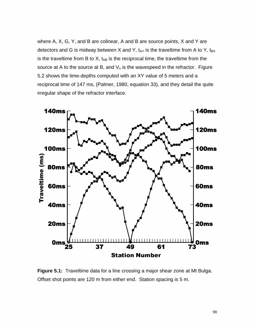
98
where A, X, G, Y, and B are colinear, A and B are source points, X and Y are
detectors and G is midway between X and Y, tAY is the traveltime from A to Y, tBX
is the traveltime from B to X, tAB is the reciprocal time, the traveltime from the
source at A to the source at B, and Vn is the wavespeed in the refractor. Figure
5.2 shows the time-depths computed with an XY value of 5 meters and a
reciprocal time of 147 ms, (Palmer, 1980, equation 33), and they detail the quite
irregular shape of the refractor interface.
Figure 5.1: Traveltime data for a line crossing a major shear zone at Mt Bulga.
Offset shot points are 120 m from either end. Station spacing is 5 m.
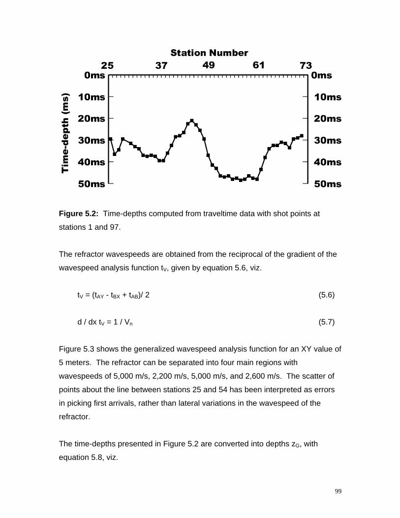
99
Figure 5.2: Time-depths computed from traveltime data with shot points at
stations 1 and 97.
The refractor wavespeeds are obtained from the reciprocal of the gradient of the
wavespeed analysis function tV, given by equation 5.6, viz.
tV = (tAY - tBX + tAB)/ 2 (5.6)
d / dx tV = 1 / Vn (5.7)
Figure 5.3 shows the generalized wavespeed analysis function for an XY value of
5 meters. The refractor can be separated into four main regions with
wavespeeds of 5,000 m/s, 2,200 m/s, 5,000 m/s, and 2,600 m/s. The scatter of
points about the line between stations 25 and 54 has been interpreted as errors
in picking first arrivals, rather than lateral variations in the wavespeed of the
refractor.
The time-depths presented in Figure 5.2 are converted into depths zG, with
equation 5.8, viz.
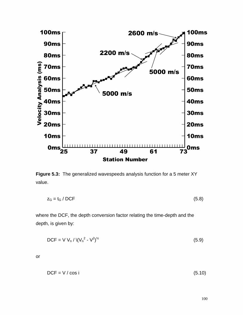
100
Figure 5.3: The generalized wavespeeds analysis function for a 5 meter XY
value.
zG = tG / DCF (5.8)
where the DCF, the depth conversion factor relating the time-depth and the
depth, is given by:
DCF = V Vn / \(Vn2 - V2)½ (5.9)
or
DCF = V / cos i (5.10)
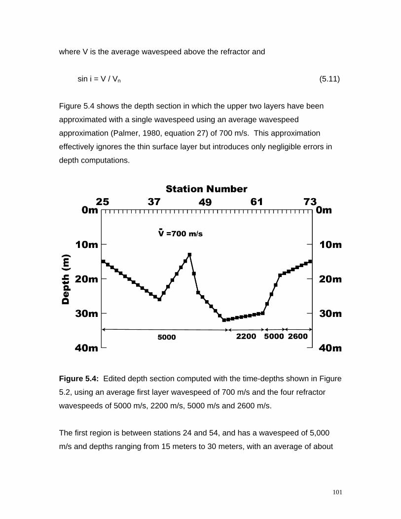
101
where V is the average wavespeed above the refractor and
sin i = V / Vn (5.11)
Figure 5.4 shows the depth section in which the upper two layers have been
approximated with a single wavespeed using an average wavespeed
approximation (Palmer, 1980, equation 27) of 700 m/s. This approximation
effectively ignores the thin surface layer but introduces only negligible errors in
depth computations.
Figure 5.4: Edited depth section computed with the time-depths shown in Figure
5.2, using an average first layer wavespeed of 700 m/s and the four refractor
wavespeeds of 5000 m/s, 2200 m/s, 5000 m/s and 2600 m/s.
The first region is between stations 24 and 54, and has a wavespeed of 5,000
m/s and depths ranging from 15 meters to 30 meters, with an average of about
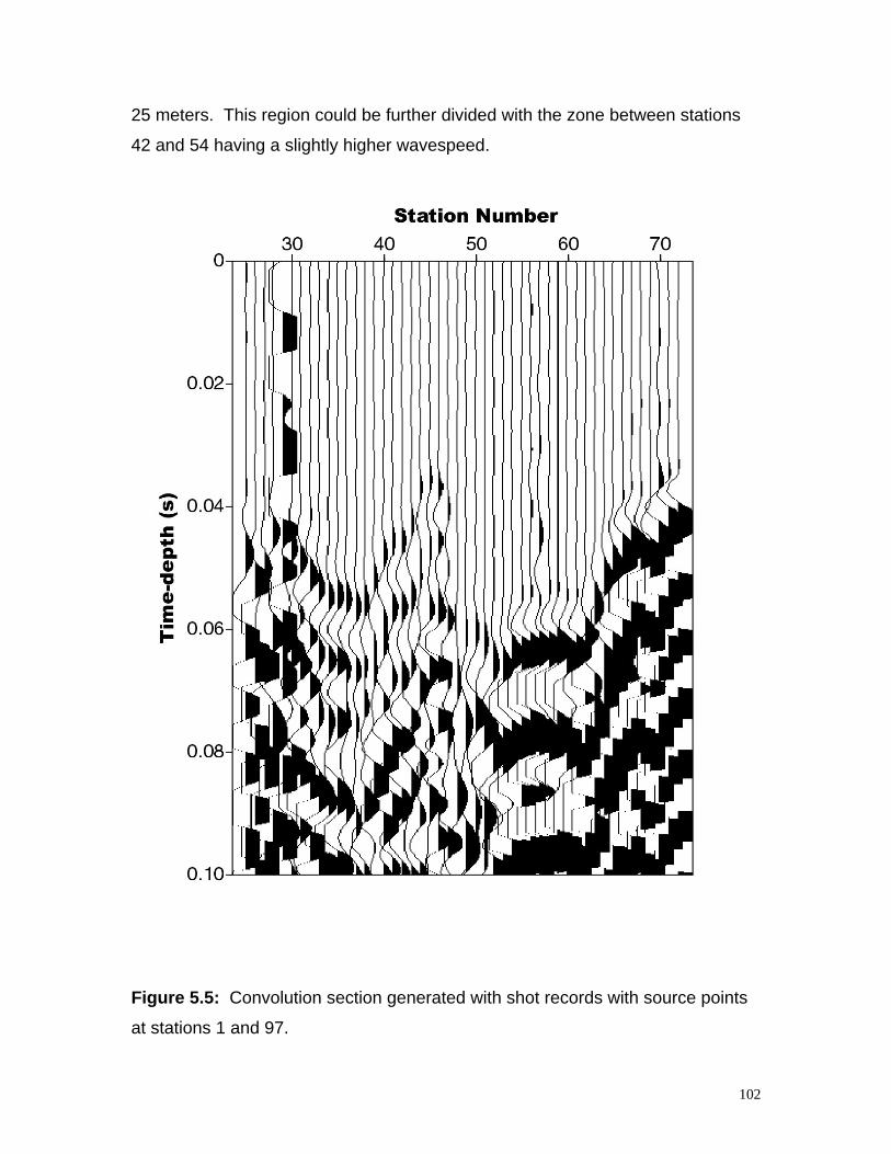
102
25 meters. This region could be further divided with the zone between stations
42 and 54 having a slightly higher wavespeed.
Figure 5.5: Convolution section generated with shot records with source points
at stations 1 and 97.
103
The second region is between stations 54 and 62. It has a wavespeed of 2,200
m/s and an average depth of over 30 meters. It corresponds with the inferred
location of the major shear zone.
The third region is between stations 62 and 67. It has a wavespeed of 5000 m/s
and depths range from 28 to 15 meters. This region is relatively narrow, and the
wavespeed is not well determined, possibly because it is associated with a major
change in depths. A re-interpretation of Figure 5.3 indicates that a lower value of
less than 4000 m/s could be assigned to this region.
The fourth region is between stations 67 and 73. It has a wavespeed of 2600
m/s and an average depth of about 15 meters.
The convolution section presented in Figure 5.5, shows the same structure as
the time-depths in Figure 5.2, and it is possible to recognize four regions with the
relative amplitudes of approximately 1, 5, 2, and 4 (Palmer, 2001; chapter 3,
Figure 3.9). These regions correspond with those determined on the basis of
refractor wavespeeds in Figure 5.3. The ratios of the wavespeeds in each region
to the average wavespeed in the overburden are 0.14, 0.32, 0.14, and 0.27. The
square of these ratios normalized to the lowest value are 1, 5.2, 1, 3.7. They are
similar to the ratios of the convolved amplitudes, except for the third region,
where a refractor wavespeed of 3540 m/s would be compatible with the observed
amplitude.
This case history provides a compelling demonstration of the correlation between
amplitudes and wavespeeds with a complex refractor exhibiting large changes in
both depth and wavespeed. Not only do major changes in wavespeed result in
marked amplitude variations, such as the contrast between the regions with
wavespeeds of 5000 m/s and 2200 m/s, but subtle changes within each region
can also be recognized. For example, the region between stations 42 and 54
104
has a slightly higher wavespeed and lower convolved amplitudes than is the case
between stations 25 and 42.
This example also demonstrates the ability of amplitudes to help resolve any
ambiguities in the determination of refractor wavespeeds. The third region of the
refractor between stations 62 and 67 is relatively narrow and has a large change
in depth. Both of these factors may affect the amplitudes and the accuracy of the
measurement of the wavespeed. A re-interpretation of the wavespeed analysis
function together with the amplitudes suggest that a lower wavespeed of
between 3540 m/s and 4000 m/s would be more appropriate for this interval.
5.5 - Conclusions
The inversion of refraction data can be ambiguous. Artifacts, such as narrow
zones with higher and lower wavespeeds can be produced where there are
changes in the depth to the refractor. In general, forward modeling does not
recognize or correct these artifacts.
The amplitudes of the refracted signals provide another means of recognizing
genuine lateral variations in wavespeed within the refractor, once the large
effects of geometric spreading are removed. This study uses the convolution of
forward and reverse seismic traces to compensate for geometrical spreading.
The refraction time section obtained in this way facilitates the correlation of
structure on the refractor interface with amplitudes, and in turn with wavespeeds
within the refractor.
The case history has large variations in depths to and wavespeeds within the
refractor and provides a searching test of the method. The regions in the
refractor recognized with the wavespeed analysis function correlate closely with
the regions recognized with the convolved amplitudes or the amplitude products.
105
Low contrasts in the wavespeeds between the refractor and the overlying layer
produce higher amplitudes than is the case with high contrasts.
This feature alone is very useful in constraining the generation of artifacts with
model-based inversion. The gross features of the interpretation model
recognizable in the convolution section should also have corresponding
expressions in the results obtained with other approaches.
For large contrasts in the wavespeeds and/or densities between the upper layer
and the refractor, the head coefficient is approximately proportional to the ratio of
the specific acoustic impedances. In turn, the amplitudes in the convolution
section are proportional to the square of this ratio because the forward and
reverse amplitudes are multiplied with convolution. This approximation is
satisfactory for three of the regions examined in the case history. Furthermore, it
supports a revision of the wavespeeds in a narrow region of the refractor to a
lower value than was initially inferred.
The convolution section is a very effective single presentation for combining the
information depicting the geometry of the refractor which is obtained with the
time-depth algorithm, and the information depicting the wavespeed in the
refractor which is usually obtained with the wavespeed analysis algorithm. It is
very rapid to generate, avoiding in particular the familiar time consuming tasks of
determining first arrival traveltimes and amplitudes. In addition, little, if any, a
priori information on upper layer or refractor wavespeeds is required, although of
course such information is essential for the generation of final depth cross
sections.
Accordingly, the convolution section is an extremely useful and convenient
presentation for inclusion in the routine processing of seismic refraction data
using any method.
106
5.6 - References
CervenY, V., and Ravindra, R., 1971, Theory of seismic head waves: University
of Toronto Press.
Heelan, P. A., 1953, On the theory of head waves: Geophysics, 18, 871-893.
O’Brien, P. N. S., 1967, The use of amplitudes in seismic refraction survey, in
Musgrave, A. W., ed., Seismic refraction prospecting: Society of Exploration
Geophysicists, 85-118.
Palmer, D., 1980, The generalized reciprocal method of seismic refraction
Interpretation: Society of Exploration Geophysicists.
Palmer, D., 1986, Refraction seismics: the lateral resolution of structure and
seismic velocity: Geophysical Press.
Palmer, D., 1991, The resolution of narrow low-velocity zones with the
generalized reciprocal method: Geophys. Prosp., 39, 1031-1060.
Palmer, D., 2001, Imaging refractors with the convolution section: Geophysics
66, 1582-1589.
Werth, G. A., 1967, Method for calculating the amplitude of the refraction arrival,
in Musgrave, A. W., Ed., Seismic refraction prospecting: Society of Exploration
Geophysicists, 119-137.
107
Chapter 6
Efficient Mapping Of Structure AndAzimuthal Anisotropy With Three
Dimensional Shallow SeismicRefraction Methods
6.1 - Summary
A three dimensional (3D) seismic refraction survey was carried out across a
shear zone.
The data were processed with the generalized reciprocal method (GRM) rather
than with tomographic inversion because of the relatively small volume of data,
the occurrence of large variations in depth to and wavespeeds within the main
refractor and the presence of azimuthal anisotropy.
The results show that there is an increase in the depth of weathering and a
decrease in wavespeed in the sub-weathering associated with the shear zone.
Although the shear zone is generally considered to be a two dimensional (2D)
feature, the significant lateral variations in both depths to and wavespeeds within
the refractor in the cross-line direction indicate that it is best treated as a 3D
target. These variations are not predictable on the basis of a 2D profile recorded
earlier.
108
The amplitudes of the refracted signals are approximately proportional to the
ratio of the specific acoustic impedances between the upper layer and the
refractor and they provide a convenient and detailed measure of apparent
azimuthal anisotropy or rock fabric. The amplitudes also contain additional
useful geological information, although some of the cross-line amplitudes could
not be completely explained.
Qualitative measures of azimuthal anisotropy are obtained from the wavespeeds
and the time-depths computed from the traveltime data with the GRM algorithms
and from the amplitudes. These three methods give similar consistent results,
with the direction of the greater wavespeed being approximately parallel to the
direction of the dominant geological strike. Furthermore, all three methods show
that the direction of the greater wavespeed is approximately orthogonal to the
direction of the dominant geological strike in one region adjacent to the shear
zone.
The in-line results show that both accurate refractor depths and wavespeeds can
be computed with moderate cross-line offsets, say less than 20 m, of shot points.
These results demonstrate that swath shooting with a number of parallel
recording lines would be adequate for 3D surveys over targets such as highways,
damsites and pipelines. Only a modest increase in shot points over the
requirements for the normal 2D program would be required in the cross-line
direction for measuring azimuthal anisotropy and rock fabric with amplitudes.
6.2 - Introduction
In the last two decades, three dimensional (3D) seismic reflection methods have
revolutionized the exploration for, and production of petroleum resources. The
improved images of the subsurface geology are a result of the recognition that
109
most geological targets are in fact three dimensional, and that it is essential to
employ spatial sampling densities and processing methods which recognize and
accommodate this reality. It is now generally accepted that in many cases, two
dimensional (2D) seismic reflection methods give an incorrect rather than an
incomplete picture of the sub-surface (Nestvold, 1992).
By contrast, 3D refraction methods (Zelt, 1998; Bennett, 1999; Deen et al, 2000)
are not very common. However, there are compelling reasons for the expedient
development of 3D shallow refraction methods for routine use in geotechnical,
environmental and groundwater applications.
Geological structures and the corresponding depths to and wavespeeds within
bedrock, can show as much variation in the cross-line direction as in the in-line
direction. In the vast majority of near-surface studies, such variations are
significant.
There is a need to address azimuthal anisotropy of wavespeeds. Anisotropy can
be caused by lamination, foliation or by the preferred orientation of joints and
cracks within the refractor, and it is another important parameter for assessing
rock strength for rippability and foundation design. However, its most important
near-surface application may be in the determination of fracture porosity in
crystalline rocks for the development of groundwater supplies for domestic and
irrigation purposes, in studies of contaminant transport especially of radioactive
wastes (Barker, 1991), the stability of rock slopes and seepage from dams, the
construction of underground rock cavities for storing water, gas, etc, and the
construction of tunnels.
The relationship between anisotropy and crack parameters has been the subject
of considerable research in the past (Crampin et al, 1980; Thomsen, 1995).
Nevertheless, there are no established approaches for the routine mapping of
these parameters with shallow geotechnical or environmental targets, although
110
radial surveys to measure azimuthal anisotropy (Bamford and Nunn, 1979; Leslie
and Lawton, 1999) represent the first steps in that direction.
6.3 - Data Processing With The GRM
This study describes the results of a 3D shallow seismic refraction survey
recorded some time ago across a shear zone at Mt Bulga in southeastern
Australia. The data are processed with a traditional approach using the
generalized reciprocal method (GRM) (Palmer, 1980; Palmer1986), rather than
with tomographic inversion for the following reasons.
The wavespeeds in the refractor range from less than 2000 m/s in the shear
zone to more than 5000 m/s in the adjacent rocks. Recent case histories (Lanz
et al, 1998), demonstrate that current tomographic inversion methods cannot yet
reliably resolve wavespeeds in the main refractor, even though over 90% of the
traveltimes originated from the refractor. In those cases where stable inversion
has been achieved, the variations in wavespeeds are generally less than about
5% (Zelt, 1998).
The volume of data is low in contrast to that generally considered desirable for
effective tomographic inversion. As a comparison, the approximately 2000
traveltimes for 120 detector positions used in this study are much less than the
more than 50,000 traveltimes for 29 detector positions used in the tomographic
analysis of Zelt and Barton, (1998). For most routine shallow refraction
investigations, the costs of recording at least an order of magnitude of additional
shot points can be prohibitive.
Model studies and case histories (Palmer, 1980; Palmer, 1991) demonstrate that
the GRM can resolve large variations in the depths to and wavespeeds within
111
refractors using considerably smaller data volumes than is the case with most
tomography programs.
Azimuthal anisotropy is rarely accommodated with most tomography programs.
Isotropy is normally assumed in order to employ as many traveltimes from as
many directions as possible in the inversion process. In addition, the traveltime
differences due to anisotropy are quite small, and are often within the accepted
range for the residuals of inversion.
In this study, the amplitudes of the refracted head waves are used to map
anisotropy. Previous studies have shown that the head coefficient, the
parameter which controls the amplitude of the refracted signal, is approximately
proportional to the ratio of the specific acoustic impedances of the overburden
and the refractor (Palmer, 2001b; chapter 5). However, the head wave
amplitudes are generally dominated by the rapid variation due to geometric
spreading. Another study (Palmer, 2001a; chapter 3), demonstrates that the
effects of geometrical spreading and dipping interfaces can be accommodated
with either the multiplication of the amplitudes of the forward and reverse traces,
or by the convolution of those traces. In this study, the ratios of the amplitude
products for pairs of shot points with varying azimuths are used as a qualitative
measure of azimuthal anisotropy.
6.4 - Survey Details
The data used in this study were acquired in approximately the same location as
a 2D set of data described previously (Palmer, 2001a; chapter 3). The survey
was carried out shortly after the area had undergone complete clearing of the
native vegetation and subsequent planting of tube stock for a pine plantation. As
a result, the survey pegs which marked out the exploration grid, had been
removed, and so the precise relationship between the two surveys is not known.
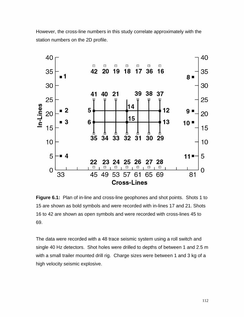
112
However, the cross-line numbers in this study correlate approximately with the
station numbers on the 2D profile.
Figure 6.1: Plan of in-line and cross-line geophones and shot points. Shots 1 to
15 are shown as bold symbols and were recorded with in-lines 17 and 21. Shots
16 to 42 are shown as open symbols and were recorded with cross-lines 45 to
69.
The data were recorded with a 48 trace seismic system using a roll switch and
single 40 Hz detectors. Shot holes were drilled to depths of between 1 and 2.5 m
with a small trailer mounted drill rig. Charge sizes were between 1 and 3 kg of a
high velocity seismic explosive.
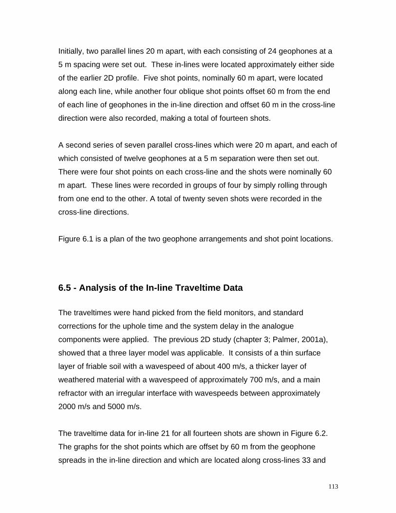
113
Initially, two parallel lines 20 m apart, with each consisting of 24 geophones at a
5 m spacing were set out. These in-lines were located approximately either side
of the earlier 2D profile. Five shot points, nominally 60 m apart, were located
along each line, while another four oblique shot points offset 60 m from the end
of each line of geophones in the in-line direction and offset 60 m in the cross-line
direction were also recorded, making a total of fourteen shots.
A second series of seven parallel cross-lines which were 20 m apart, and each of
which consisted of twelve geophones at a 5 m separation were then set out.
There were four shot points on each cross-line and the shots were nominally 60
m apart. These lines were recorded in groups of four by simply rolling through
from one end to the other. A total of twenty seven shots were recorded in the
cross-line directions.
Figure 6.1 is a plan of the two geophone arrangements and shot point locations.
6.5 - Analysis of the In-line Traveltime Data
The traveltimes were hand picked from the field monitors, and standard
corrections for the uphole time and the system delay in the analogue
components were applied. The previous 2D study (chapter 3; Palmer, 2001a),
showed that a three layer model was applicable. It consists of a thin surface
layer of friable soil with a wavespeed of about 400 m/s, a thicker layer of
weathered material with a wavespeed of approximately 700 m/s, and a main
refractor with an irregular interface with wavespeeds between approximately
2000 m/s and 5000 m/s.
The traveltime data for in-line 21 for all fourteen shots are shown in Figure 6.2.
The graphs for the shot points which are offset by 60 m from the geophone
spreads in the in-line direction and which are located along cross-lines 33 and
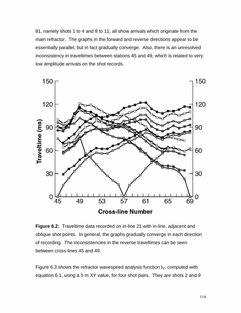
114
81, namely shots 1 to 4 and 8 to 11, all show arrivals which originate from the
main refractor. The graphs in the forward and reverse directions appear to be
essentially parallel, but in fact gradually converge. Also, there is an unresolved
inconsistency in traveltimes between stations 45 and 49, which is related to very
low amplitude arrivals on the shot records.
Figure 6.2: Traveltime data recorded on in-line 21 with in-line, adjacent and
oblique shot points. In general, the graphs gradually converge in each direction
of recording. The inconsistencies in the reverse traveltimes can be seen
between cross-lines 45 and 49.
Figure 6.3 shows the refractor wavespeed analysis function tV, computed with
equation 6.1, using a 5 m XY value, for four shot pairs. They are shots 2 and 9
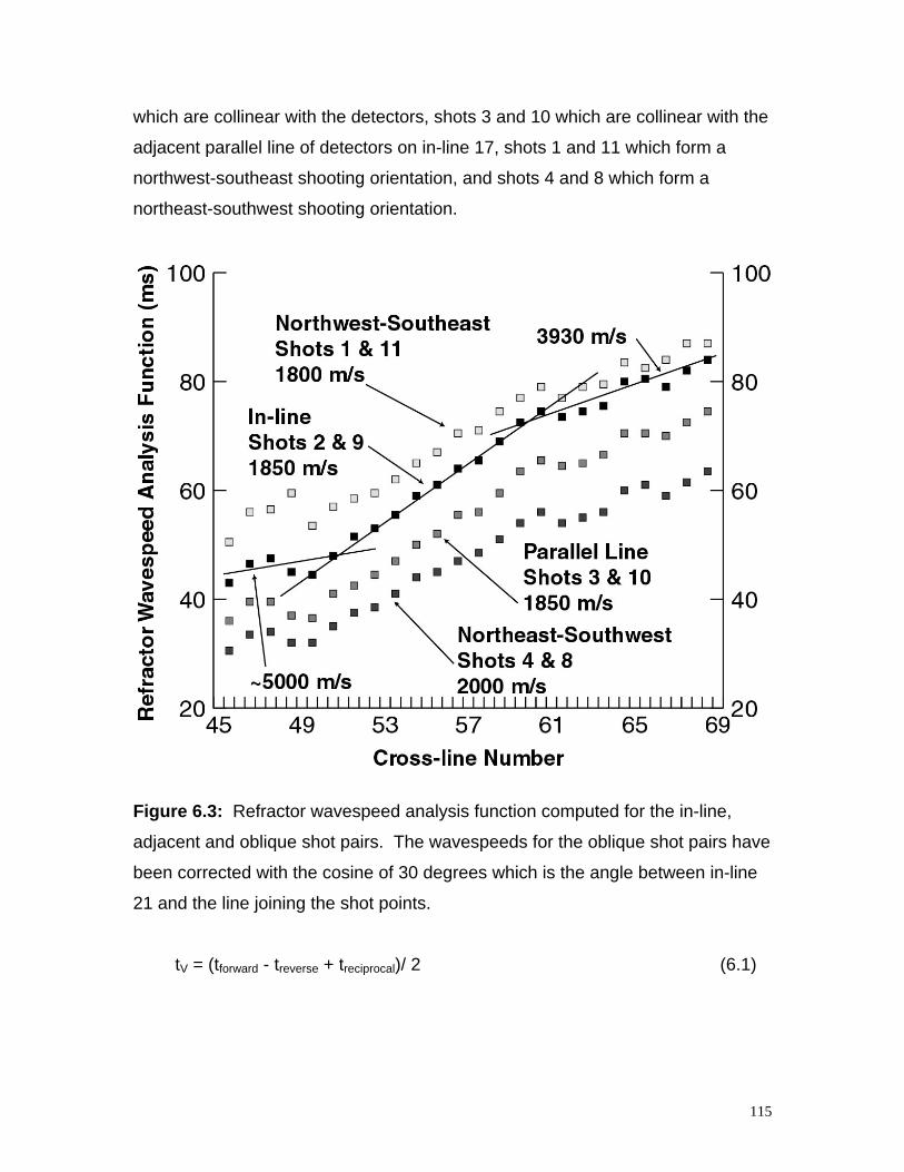
115
which are collinear with the detectors, shots 3 and 10 which are collinear with the
adjacent parallel line of detectors on in-line 17, shots 1 and 11 which form a
northwest-southeast shooting orientation, and shots 4 and 8 which form a
northeast-southwest shooting orientation.
Figure 6.3: Refractor wavespeed analysis function computed for the in-line,
adjacent and oblique shot pairs. The wavespeeds for the oblique shot pairs have
been corrected with the cosine of 30 degrees which is the angle between in-line
21 and the line joining the shot points.
tV = (tforward - treverse + treciprocal)/ 2 (6.1)
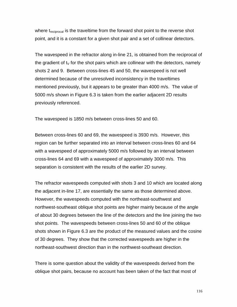
116
where treciprocal is the traveltime from the forward shot point to the reverse shot
point, and it is a constant for a given shot pair and a set of collinear detectors.
The wavespeed in the refractor along in-line 21, is obtained from the reciprocal of
the gradient of tV for the shot pairs which are collinear with the detectors, namely
shots 2 and 9. Between cross-lines 45 and 50, the wavespeed is not well
determined because of the unresolved inconsistency in the traveltimes
mentioned previously, but it appears to be greater than 4000 m/s. The value of
5000 m/s shown in Figure 6.3 is taken from the earlier adjacent 2D results
previously referenced.
The wavespeed is 1850 m/s between cross-lines 50 and 60.
Between cross-lines 60 and 69, the wavespeed is 3930 m/s. However, this
region can be further separated into an interval between cross-lines 60 and 64
with a wavespeed of approximately 5000 m/s followed by an interval between
cross-lines 64 and 69 with a wavespeed of approximately 3000 m/s. This
separation is consistent with the results of the earlier 2D survey.
The refractor wavespeeds computed with shots 3 and 10 which are located along
the adjacent in-line 17, are essentially the same as those determined above.
However, the wavespeeds computed with the northeast-southwest and
northwest-southeast oblique shot points are higher mainly because of the angle
of about 30 degrees between the line of the detectors and the line joining the two
shot points. The wavespeeds between cross-lines 50 and 60 of the oblique
shots shown in Figure 6.3 are the product of the measured values and the cosine
of 30 degrees. They show that the corrected wavespeeds are higher in the
northeast-southwest direction than in the northwest-southeast direction.
There is some question about the validity of the wavespeeds derived from the
oblique shot pairs, because no account has been taken of the fact that most of
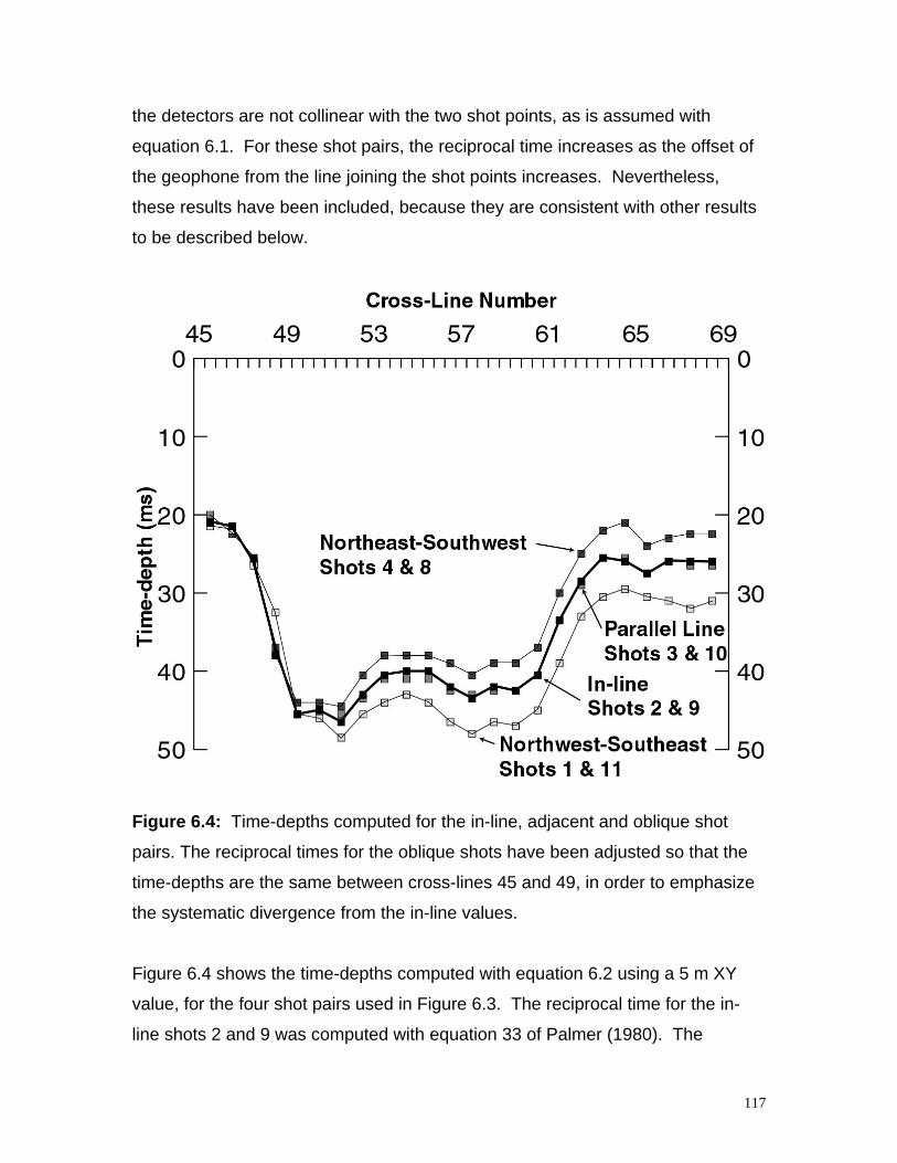
117
the detectors are not collinear with the two shot points, as is assumed with
equation 6.1. For these shot pairs, the reciprocal time increases as the offset of
the geophone from the line joining the shot points increases. Nevertheless,
these results have been included, because they are consistent with other results
to be described below.
Figure 6.4: Time-depths computed for the in-line, adjacent and oblique shot
pairs. The reciprocal times for the oblique shots have been adjusted so that the
time-depths are the same between cross-lines 45 and 49, in order to emphasize
the systematic divergence from the in-line values.
Figure 6.4 shows the time-depths computed with equation 6.2 using a 5 m XY
value, for the four shot pairs used in Figure 6.3. The reciprocal time for the in-
line shots 2 and 9 was computed with equation 33 of Palmer (1980). The
118
reciprocal times for the other shot pairs could not be derived as conveniently, and
they have been adjusted until the differences in the time-depths between cross-
lines 45 and 49 were minimized. This facilitates the recognition of the systematic
divergence of the time-depths for the oblique shot pairs from the collinear values.
time-depth = (tforward + treverse - treciprocal)/2. (6.2)
The increase in the time-depths between cross-lines 50 and 60 corresponds to
the region in the refractor with the low wavespeed.
The systematic divergence of the time-depths computed with the oblique shot
pairs from cross-line 49 to cross-line 69, can be employed as a qualitative
measure of azimuthal anisotropy in the following way.
The time-depths tG, are related to the depths zG, with equation 6.3,
zG = tG / DCF (6.3)
where the DCF, the depth conversion factor relating the time-depth and the
depth, is given by:
DCF = V Vn / (Vn2 - V2)½ (6.4)
or
DCF = V / cos i (6.5)
where V is the average wavespeed above the refractor and
sin i = V / Vn (6.6)
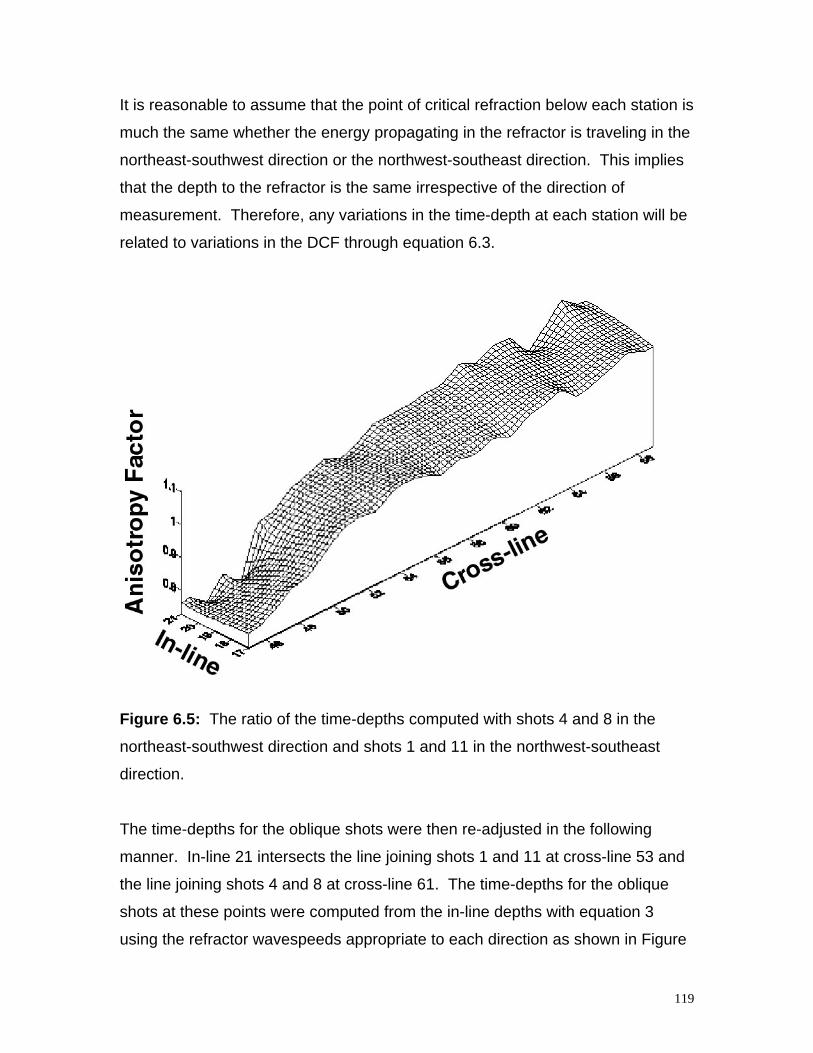
119
It is reasonable to assume that the point of critical refraction below each station is
much the same whether the energy propagating in the refractor is traveling in the
northeast-southwest direction or the northwest-southeast direction. This implies
that the depth to the refractor is the same irrespective of the direction of
measurement. Therefore, any variations in the time-depth at each station will be
related to variations in the DCF through equation 6.3.
Figure 6.5: The ratio of the time-depths computed with shots 4 and 8 in the
northeast-southwest direction and shots 1 and 11 in the northwest-southeast
direction.
The time-depths for the oblique shots were then re-adjusted in the following
manner. In-line 21 intersects the line joining shots 1 and 11 at cross-line 53 and
the line joining shots 4 and 8 at cross-line 61. The time-depths for the oblique
shots at these points were computed from the in-line depths with equation 3
using the refractor wavespeeds appropriate to each direction as shown in Figure
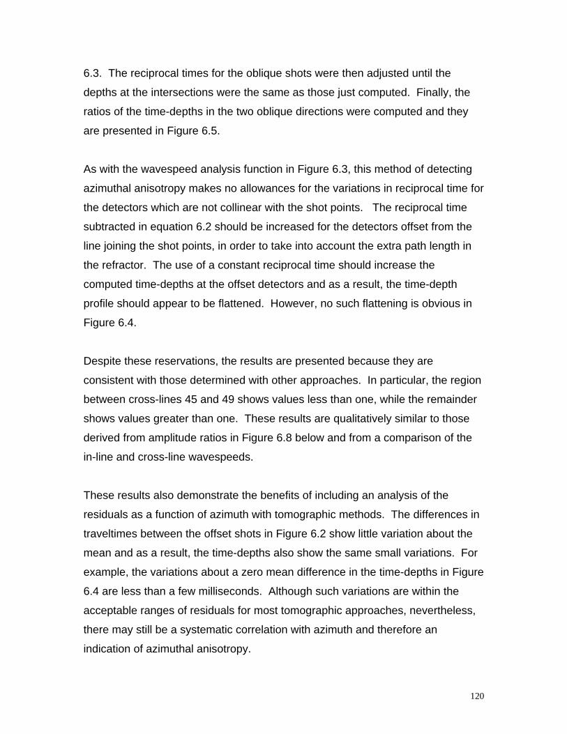
120
6.3. The reciprocal times for the oblique shots were then adjusted until the
depths at the intersections were the same as those just computed. Finally, the
ratios of the time-depths in the two oblique directions were computed and they
are presented in Figure 6.5.
As with the wavespeed analysis function in Figure 6.3, this method of detecting
azimuthal anisotropy makes no allowances for the variations in reciprocal time for
the detectors which are not collinear with the shot points. The reciprocal time
subtracted in equation 6.2 should be increased for the detectors offset from the
line joining the shot points, in order to take into account the extra path length in
the refractor. The use of a constant reciprocal time should increase the
computed time-depths at the offset detectors and as a result, the time-depth
profile should appear to be flattened. However, no such flattening is obvious in
Figure 6.4.
Despite these reservations, the results are presented because they are
consistent with those determined with other approaches. In particular, the region
between cross-lines 45 and 49 shows values less than one, while the remainder
shows values greater than one. These results are qualitatively similar to those
derived from amplitude ratios in Figure 6.8 below and from a comparison of the
in-line and cross-line wavespeeds.
These results also demonstrate the benefits of including an analysis of the
residuals as a function of azimuth with tomographic methods. The differences in
traveltimes between the offset shots in Figure 6.2 show little variation about the
mean and as a result, the time-depths also show the same small variations. For
example, the variations about a zero mean difference in the time-depths in Figure
6.4 are less than a few milliseconds. Although such variations are within the
acceptable ranges of residuals for most tomographic approaches, nevertheless,
there may still be a systematic correlation with azimuth and therefore an
indication of azimuthal anisotropy.
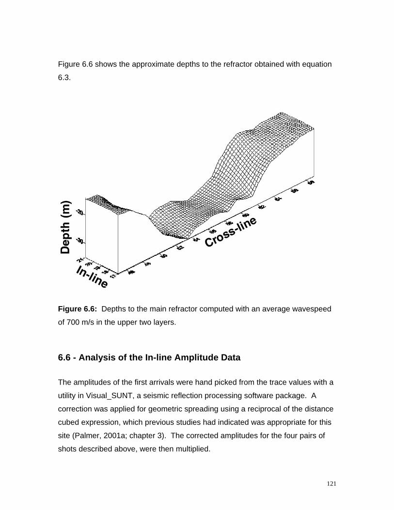
121
Figure 6.6 shows the approximate depths to the refractor obtained with equation
6.3.
Figure 6.6: Depths to the main refractor computed with an average wavespeed
of 700 m/s in the upper two layers.
6.6 - Analysis of the In-line Amplitude Data
The amplitudes of the first arrivals were hand picked from the trace values with a
utility in Visual_SUNT, a seismic reflection processing software package. A
correction was applied for geometric spreading using a reciprocal of the distance
cubed expression, which previous studies had indicated was appropriate for this
site (Palmer, 2001a; chapter 3). The corrected amplitudes for the four pairs of
shots described above, were then multiplied.
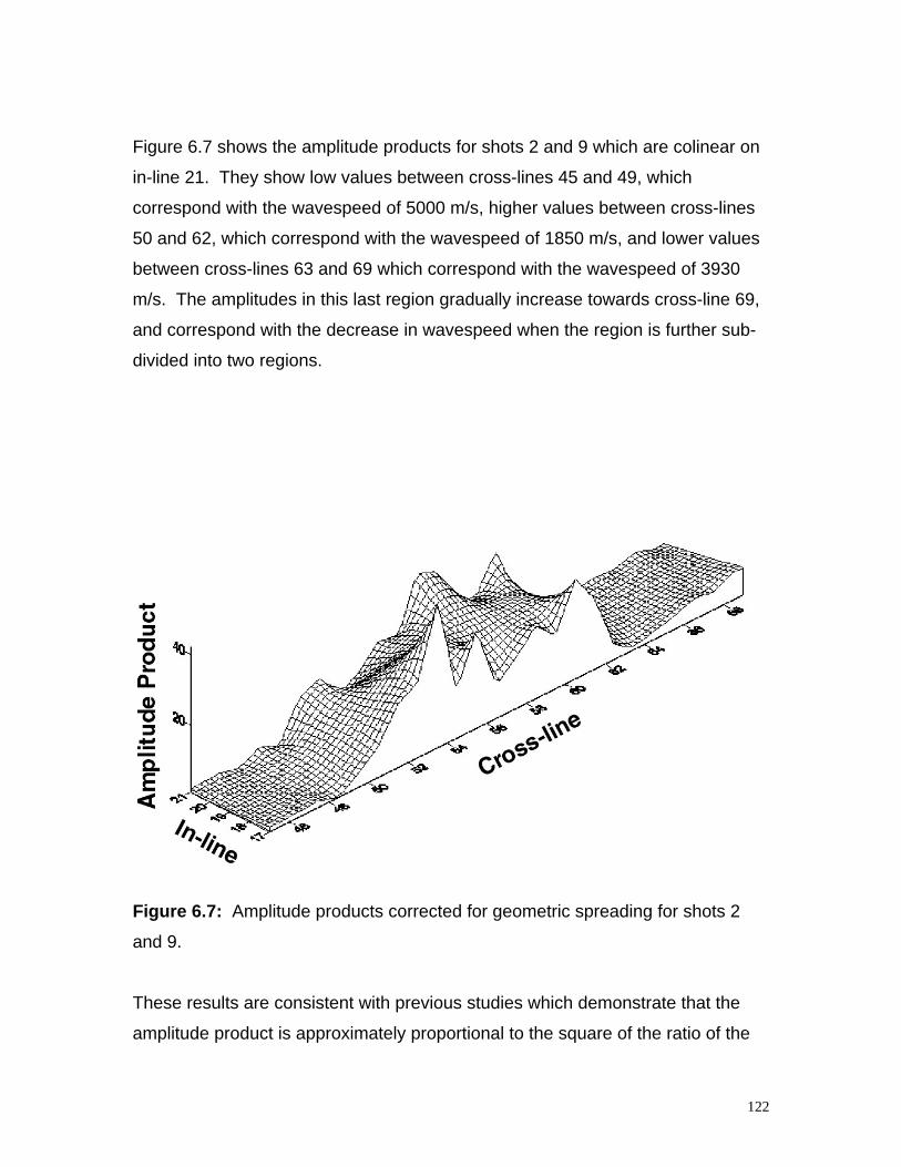
122
Figure 6.7 shows the amplitude products for shots 2 and 9 which are colinear on
in-line 21. They show low values between cross-lines 45 and 49, which
correspond with the wavespeed of 5000 m/s, higher values between cross-lines
50 and 62, which correspond with the wavespeed of 1850 m/s, and lower values
between cross-lines 63 and 69 which correspond with the wavespeed of 3930
m/s. The amplitudes in this last region gradually increase towards cross-line 69,
and correspond with the decrease in wavespeed when the region is further sub-
divided into two regions.
Figure 6.7: Amplitude products corrected for geometric spreading for shots 2
and 9.
These results are consistent with previous studies which demonstrate that the
amplitude product is approximately proportional to the square of the ratio of the
123
specific acoustic impedances of the overburden and the refractor (chapter 5;
Palmer, 2001b). Since the wavespeeds in the layers above the main refractor
exhibit little lateral variation in the in-line direction, the amplitudes are essentially
a function of the wavespeeds and densities in the refractor.
The amplitudes of the other shot pairs show the same general pattern, as well as
the detailed features such as the higher values at cross-lines 54, 56, 59 and 61
on line 17. These variations can be attributed to changes in the coupling of the
detectors, or near-surface changes in the wavespeeds.
Figure 6.8: An apparent anisotropy factor obtained from the square root of the
ratio of the corrected amplitudes for the two pairs of oblique shots.
Figure 6.8 shows the square root of the ratio of the amplitudes obtained with
shots 4 and 8 in the northeast-southwest direction to the amplitudes obtained
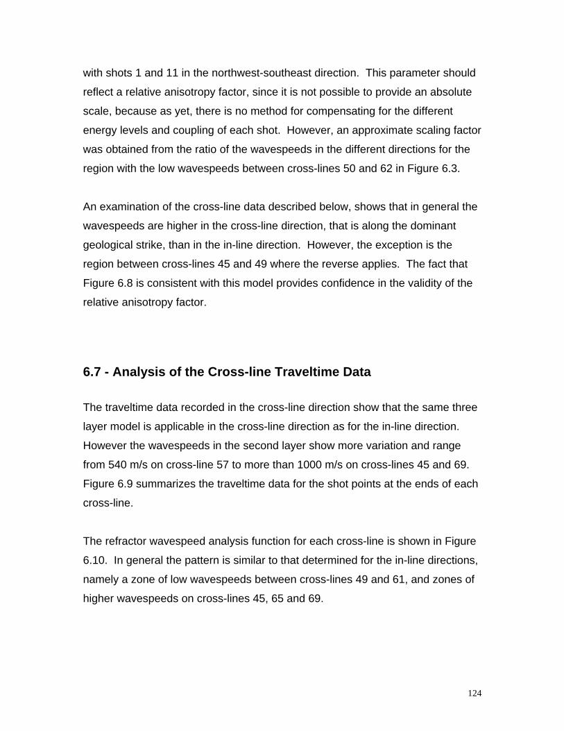
124
with shots 1 and 11 in the northwest-southeast direction. This parameter should
reflect a relative anisotropy factor, since it is not possible to provide an absolute
scale, because as yet, there is no method for compensating for the different
energy levels and coupling of each shot. However, an approximate scaling factor
was obtained from the ratio of the wavespeeds in the different directions for the
region with the low wavespeeds between cross-lines 50 and 62 in Figure 6.3.
An examination of the cross-line data described below, shows that in general the
wavespeeds are higher in the cross-line direction, that is along the dominant
geological strike, than in the in-line direction. However, the exception is the
region between cross-lines 45 and 49 where the reverse applies. The fact that
Figure 6.8 is consistent with this model provides confidence in the validity of the
relative anisotropy factor.
6.7 - Analysis of the Cross-line Traveltime Data
The traveltime data recorded in the cross-line direction show that the same three
layer model is applicable in the cross-line direction as for the in-line direction.
However the wavespeeds in the second layer show more variation and range
from 540 m/s on cross-line 57 to more than 1000 m/s on cross-lines 45 and 69.
Figure 6.9 summarizes the traveltime data for the shot points at the ends of each
cross-line.
The refractor wavespeed analysis function for each cross-line is shown in Figure
6.10. In general the pattern is similar to that determined for the in-line directions,
namely a zone of low wavespeeds between cross-lines 49 and 61, and zones of
higher wavespeeds on cross-lines 45, 65 and 69.
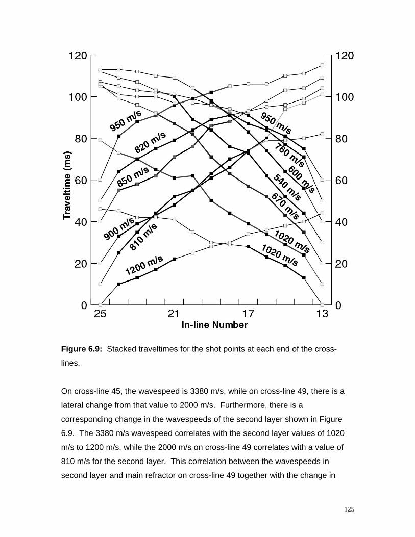
125
Figure 6.9: Stacked traveltimes for the shot points at each end of the cross-
lines.
On cross-line 45, the wavespeed is 3380 m/s, while on cross-line 49, there is a
lateral change from that value to 2000 m/s. Furthermore, there is a
corresponding change in the wavespeeds of the second layer shown in Figure
6.9. The 3380 m/s wavespeed correlates with the second layer values of 1020
m/s to 1200 m/s, while the 2000 m/s on cross-line 49 correlates with a value of
810 m/s for the second layer. This correlation between the wavespeeds in
second layer and main refractor on cross-line 49 together with the change in
126
refractor wavespeeds on the two in-line profiles at cross-line 50 are consistent
with a lateral change in wavespeed occurring on cross-line 49. The significance
of this result is that a major change in refractor wavespeed has been resolved
along cross-line 49, even though the contact between the two zones is probably
not orthogonal to cross-line 49. Theoretical studies (Sjogren, 1984, p168-173)
have predicted that there should be errors in the determination of accurate
refractor wavespeeds.
The lateral change in the wavespeed on cross-line 49 also provides an
explanation for the inconsistent traveltimes obtained on the in-line profiles with
the shot points on cross-line 81. The seismic trace consists of a low amplitude
early arrival from the high wavespeed zone, followed by the high amplitude later
arrival from the adjacent low wavespeed zone. It is possible that one of these
arrivals may be a side swipe.
The wavespeed of 3380 m/s determined in the cross-line direction is significantly
less than the value of about 5000 m/s determined previously with the 2D profile
in the in-line direction. It contrasts with the remainder of the survey area, in
which the wavespeeds are greater in the cross-line direction. However it is
consistent with qualitative measures of azimuthal anisotropy obtained with time-
depth ratios in Figure 6.5 and with amplitude ratios in Figure 6.8.
The wavespeed of 2000 m/s between cross-lines 53 and 61 is 7.5% larger than
the value of 1850 m/s measured in the in-line direction.
On cross-lines 65 and 69, the wavespeed is 6500 m/s between in-lines 19 and
21 and 2000 m/s to 2100 m/s elsewhere. Although the accuracy of the
wavespeed in this center interval is not high because it is measured over a
limited number of points, it is still higher than the in-line value of 3930 m/s
determined between cross-lines 60 and 69.
127
Figure 6.10: Stacked wavespeed analysis function for the offset shots for cross-
lines 45 to 69.
These results are a compelling demonstration that there can be important 3D
effects even with a nominally 2D geological structure. The lateral change in
wavespeeds on cross-line 49 generates inconsistent arrivals on the in-line data
which are more readily explained with the cross-line data. In addition, the rock
fabric in the region between cross-lines 45 and 49, as measured with the
apparent anisotropy factor, is approximately orthogonal to the dominant
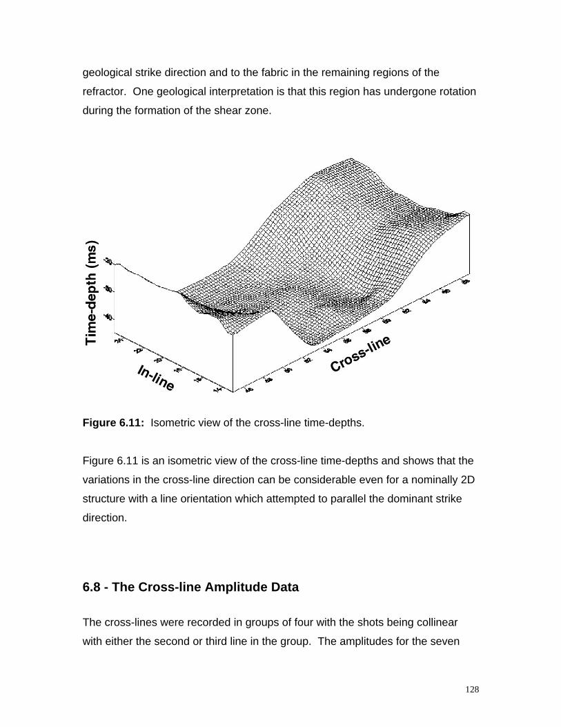
128
geological strike direction and to the fabric in the remaining regions of the
refractor. One geological interpretation is that this region has undergone rotation
during the formation of the shear zone.
Figure 6.11: Isometric view of the cross-line time-depths.
Figure 6.11 is an isometric view of the cross-line time-depths and shows that the
variations in the cross-line direction can be considerable even for a nominally 2D
structure with a line orientation which attempted to parallel the dominant strike
direction.
6.8 - The Cross-line Amplitude Data
The cross-lines were recorded in groups of four with the shots being collinear
with either the second or third line in the group. The amplitudes for the seven
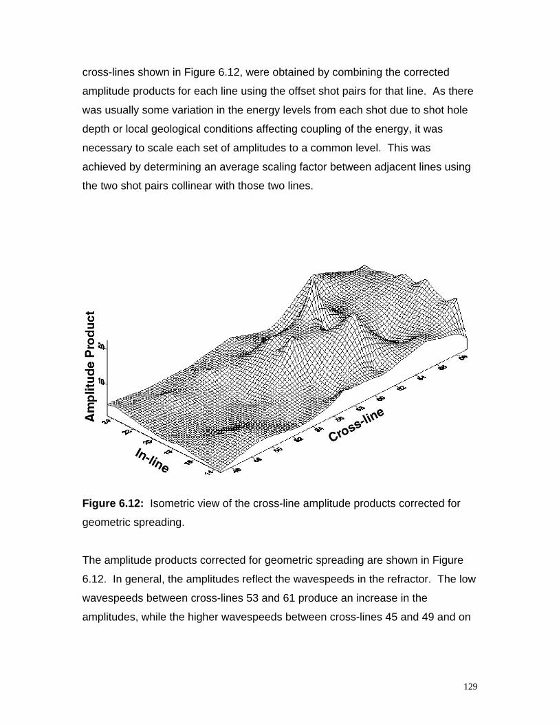
129
cross-lines shown in Figure 6.12, were obtained by combining the corrected
amplitude products for each line using the offset shot pairs for that line. As there
was usually some variation in the energy levels from each shot due to shot hole
depth or local geological conditions affecting coupling of the energy, it was
necessary to scale each set of amplitudes to a common level. This was
achieved by determining an average scaling factor between adjacent lines using
the two shot pairs collinear with those two lines.
Figure 6.12: Isometric view of the cross-line amplitude products corrected for
geometric spreading.
The amplitude products corrected for geometric spreading are shown in Figure
6.12. In general, the amplitudes reflect the wavespeeds in the refractor. The low
wavespeeds between cross-lines 53 and 61 produce an increase in the
amplitudes, while the higher wavespeeds between cross-lines 45 and 49 and on
130
cross-line 65 produce lower amplitudes. However, there are a number of
departures from this trend where a detailed correlation is made.
On cross-line 45, there is a gradual increase in amplitude from in-line 13 to in-line
25, which is consistent with an increase in the wavespeed in the overlaying layer
from 1020 m/s to 1200 m/s. On cross-line 49, the decrease in wavespeed in the
refractor from 3380 m/s to 2000 m/s is matched with a decrease in the
wavespeed in the overlaying layer from 1020 m/s to 810 m/s, resulting in only a
minor increase in amplitudes.
There is no obvious explanation for the decrease in amplitudes at each end of
cross-lines 53 to 61. While the higher amplitudes in the center of each line
correlate with the low refractor wavespeeds, there is little evidence for any
significant variation in wavespeeds in the cross-line direction.
Variations in topography and density might provide an explanation. The
topography along the in-lines 17 and 21 is lower than that of the surrounding
survey area and there is an ephemeral creek located across the southeastern
corner. Accordingly, the edges of the survey area may have lower moisture
levels and therefore lower densities in the second layer. Furthermore, no
account has been taken of shear wavespeeds, which also affect the head
coefficient.
The gradual increase in amplitudes on cross-lines 53 to 61 along in-line 13
correlates with an overall increase of wavespeeds in the second layer from about
600 m/s to about 800 m/s. However, these values are much the same as the in-
line values of about 700 m/s, and so do not provide a complete explanation for
the decrease in amplitudes at each end of cross-lines 53 to 61.
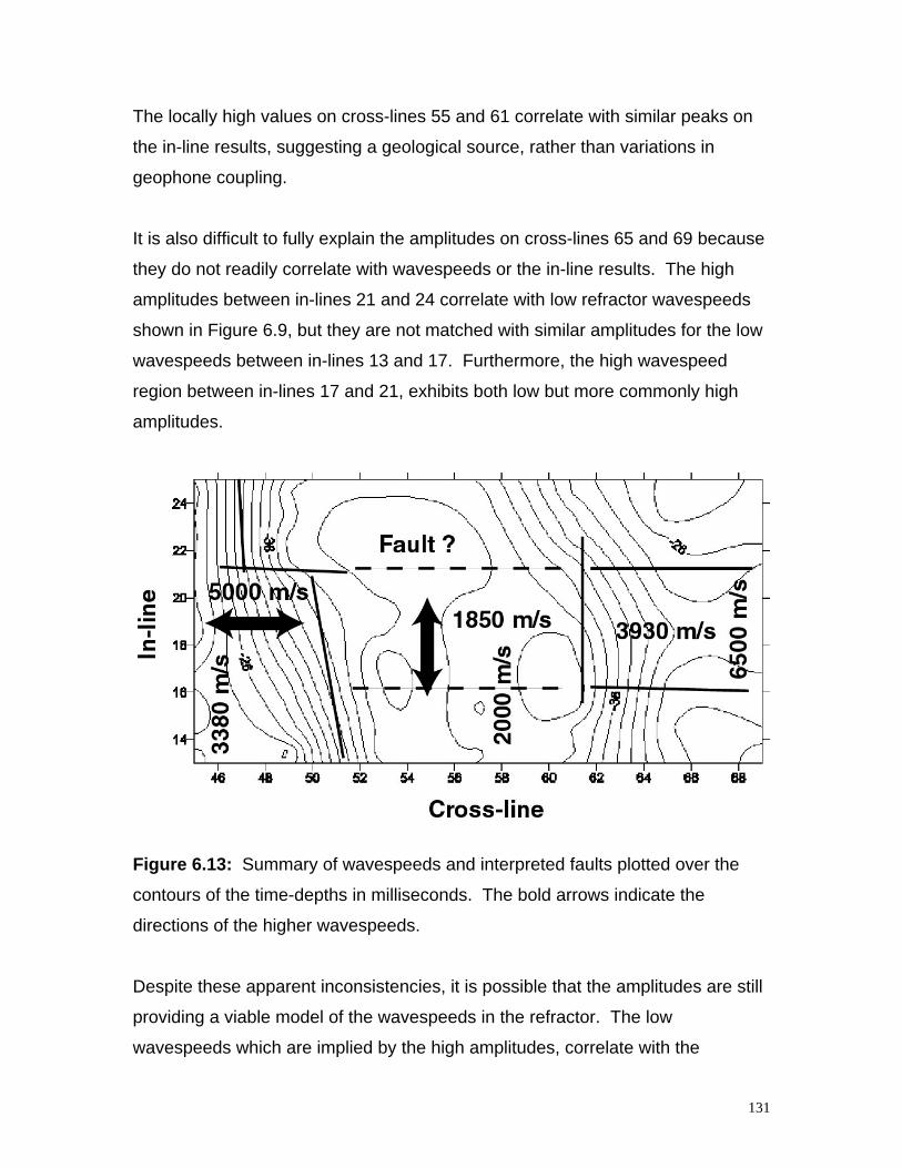
131
The locally high values on cross-lines 55 and 61 correlate with similar peaks on
the in-line results, suggesting a geological source, rather than variations in
geophone coupling.
It is also difficult to fully explain the amplitudes on cross-lines 65 and 69 because
they do not readily correlate with wavespeeds or the in-line results. The high
amplitudes between in-lines 21 and 24 correlate with low refractor wavespeeds
shown in Figure 6.9, but they are not matched with similar amplitudes for the low
wavespeeds between in-lines 13 and 17. Furthermore, the high wavespeed
region between in-lines 17 and 21, exhibits both low but more commonly high
amplitudes.
Figure 6.13: Summary of wavespeeds and interpreted faults plotted over the
contours of the time-depths in milliseconds. The bold arrows indicate the
directions of the higher wavespeeds.
Despite these apparent inconsistencies, it is possible that the amplitudes are still
providing a viable model of the wavespeeds in the refractor. The low
wavespeeds which are implied by the high amplitudes, correlate with the
132
separation of the region between cross-lines 60 and 69 into two intervals with
wavespeed of approximately 5000 m/s and 3000 m/s, and with a wavespeed of
2600 m/s detected on the earlier 2D data between cross-lines 67 and 73.
Figure 6.13 is a summary of the wavespeeds in the in-line and cross-line
directions plotted over a contour map of the time-depths. The boundaries of the
regions with different wavespeeds are interpreted as faults. An additional fault
along in-line 17 might also be inferred on the basis of the cross-line amplitudes.
Although this discussion has focused on the variations in amplitudes due to
variations in wavespeeds, it is recognized that other factors, such as inelastic
attenuation, can affect amplitudes. The inelastic attenuation in the refractor at
each detector for a given shot pair, is reduced to a constant amount with the
amplitude product or convolution and therefore, it is not a significant factor. The
inelastic attenuation in the overburden is not compensated with the amplitude
product, and it may be an important factor in lossy media. However, in this case
history, the travel path in the overburden is less than two times the dominant
wavelength of the seismic energy (700 m/s / 35 Hz), and is considered to be a
second order effect.
6.9 - Discussion and Conclusions
The results of this study are a convincing demonstration of the benefits of 3D
shallow refraction methods. Although the shear zone at Mt Bulga is considered
to be a 2D structure, the significant spatial variations in depths, wavespeeds and
azimuthal anisotropy demonstrate that it is best viewed as a 3D target.
The depths to the refractor show considerable variation in the cross-line direction
as well as in the in-line direction. There is a general increase in depths which is
associated with the lower wavespeeds of 1850 m/s to 2000 m/s between cross-
133
lines 49 and 61. However, the increase in depths between in-lines 20 and 25 on
cross-line 49 could not be confidently predicted on the basis of the results from
either the earlier 2D profile or the two in-line profiles in this study. Similarly, the
lateral variations in wavespeeds on cross-lines 65 and 69 also require the
additional coverage in the cross-line direction to be detected and resolved.
In general, the amplitudes correlate with the ratio of the wavespeeds between the
refractor and the layer above. However, there are a number of anomalies in the
cross-line results for which as yet there are no obvious explanations. The
geology of the survey area is quite complex and it is probable that drilling or
excavation would be required to obtain a complete explanation of the observed
amplitudes.
The amplitude ratios provide a convenient approach to determining azimuthal
anisotropy. The qualitative correlation between the measures of azimuthal
anisotropy obtained with wavespeeds, time-depths and amplitude ratios provides
confidence in the validity of the results. This is especially the case with the
region between cross-line 45 and 49 where the direction of the maximum
wavespeed is approximately orthogonal to that for the remainder of the survey
area and to the dominant geological strike direction.
A major benefit of using amplitudes as a measure of the wavespeeds and
therefore anisotropy, is that a value can be determined at each detector, whereas
several collinear detectors are usually required if traveltimes are employed. In
addition, it is probable that the amplitudes may be a more sensitive measure of
anisotropy than traveltimes.
There were a number of difficulties in combining some of the in-line and cross-
line amplitude results. This suggests that data be recorded in a single pass
using several parallel lines of detectors, rather than with a number separate
recording setups.
134
The results of this study also show that shots laterally offset by up to 20 m still
produce results similar to the in-line shots. Therefore, a single line of shot points
together with a number of parallel recording lines, would be efficacious for
recording 3D refraction data along narrow swaths. A minimum of three parallel
lines is suggested, while five or more would give better cross-line determinations
of wavespeeds with the traveltime data.
Such a recording program would be suitable for many types of geotechnical
investigations as for example with highways and damsites, which require only
relatively limited coverage in the cross-line direction. Accordingly, the benefits of
the additional sampling in the cross-line direction can be achieved without a
commensurate increase in the number of shot points. Typically, an increase of
about 100% over an equivalent 2D program may be sufficient.
The refractor mapped in this study has large spatial variations in depths,
wavespeeds and azimuthal anisotropy and therefore it provides a searching test
of any approach seeking to resolve each of these parameters. The results of this
study demonstrate that simple and efficient 3D refraction methods using the
GRM can provide more useful geological interpretations than would be the case
with even detailed 2D approaches.
6.10 - References
Bamford, D., and Nunn, K. R., 1979, In-situ seismic measurements of crack
anisotropy in the Carboniferous limestone of North-west England: Geophys.
Prosp., 27, 322-338.
Barker, J. A., 1991, Transport in fractured rock, in Downing, R. A., and Wilkinson,
W. B., eds., Applied groundwater hydrology: Clarendon Press, 199-216.
135
Bennett, G., 1999, 3-D seismic refraction for deep exploration targets: The
Leading Edge, 18, 186-191.
Crampin, S., McGonigle, R., and Bamford, D., 1980, Estimating crack
parameters from observations of P-wave velocity anisotropy: Geophysics, 45,
345-360.
Deen, T. J., Gohl, K., Leslie, C., Papp, E., and Wake-Dyster, K., 2000, Seismic
refraction inversion of a palaeochannel system in the Lachlan Fold Belt, Central
New South Wales: Explor. Geophys., 31, 389-393.
Lanz, E., Maurer, H., and Green, A. G., 1998, Refraction tomography over a
buried waste disposal site: Geophysics, 63, 1414-1433.
Leslie, J. M., and Lawton, D. C., 1999, A refraction-seismic field study to
determine the anisotropic parameters of shales: Geophysics, 64, 1247-1252.
Nestvold, E. O., 1992, 3-D seismic: is the promise fulfilled?: The Leading Edge,
11, 12-19.
Palmer, D., 1980, The generalized reciprocal method of seismic refraction
interpretation: Society of Exploration Geophysicists.
Palmer, D., 1986, Refraction seismics - the lateral resolution of structure and
seismic velocity: Geophysical Press.
Palmer, D., 1991, The resolution of narrow low-velocity zones with the
generalized reciprocal method: Geophys. Prosp., 39, 1031-1060.
136
Palmer, D., 2001a, Imaging refractors with convolution: Geophysics 66, 1582-
1589.
Palmer, D., 2001b, Resolving refractor ambiguities with amplitudes: Geophysics
66, 1590-1593.
Sjogren, B., 1984, Shallow refraction seismics: Chapman and Hall.
Thomsen, L., 1995, Elastic anisotropy due to aligned cracks in porous rock:
Geophys. Prosp., 43, 805-829.
Zelt, C. A., and Barton, P. J., 1998, 3D seismic refraction tomography: a
comparison of two methods applied to data from the Faeroe Basin: J. Geophy.
Res., 103, 7187-7210.
Zelt, C. A., 1998, Lateral velocity resolution from 3-D seismic refraction data:
Geophysical Journal International, 135, 1101-1112.
137
Chapter 7
Effects Of Near-Surface LateralVariations On Refraction Amplitudes
7.1 - Summary
Increases in refracted amplitudes not related to changes in the head coefficient
are usually associated with increases in traveltimes in the near-surface layers,
while decreases in amplitudes are associated with decreases in traveltimes.
These correlations demonstrate that the amplitude variations are related to
variations in the near surface geology, rather than to variations in the coupling of
the detectors with the ground.
The change in amplitude can be described with the transmission coefficient of
the Zoeppritz equations. Correction factors can be applied for those surface
conditions which are sufficiently extensive to permit the measurement of the
wavespeed. Where this is not possible, then the lowest amplitude or amplitude
product is representative of the head coefficient for the main refractor.
138
7.2 - Introduction
The generation of a refraction time section through the convolution of forward
and reverse seismic traces (Palmer, 2001a), provides a powerful and convenient
approach to resolving some of the ambiguities in the inversion of shallow seismic
refraction data (Palmer, 2001b). 2D and 3D case histories demonstrate that the
approach is efficacious with refractors exhibiting large variations in depths and
wavespeeds. The head coefficient is approximately the ratio of the specific
acoustic impedance in the upper layer to that in the refractor, while amplitudes in
the convolution section are the square of that ratio.
However, there can be geological situations where the refraction amplitudes are
not predicted by the head coefficient or its approximations. These situations
include lateral variations in the near surface layers and/or variations in the
coupling of the geophones with the ground.
The coupling of geophones, especially with the standard single geophone per
trace of most shallow seismic refraction operations, is a ubiquitous concern with
quantitative analysis of refraction amplitudes. Pieuchot (1984) reviewed earlier
work (Bycroft, 1956; Fail et al, 1962; Lamer, 1970), in which the effects of the
weight and diameter of geophones on coupling were considered. He concluded
that the size of modern geophones was adequate to produce satisfactory
coupling, and that the common geophone spike lengths of 50 mm to 100 mm
further guaranteed satisfactory coupling. Field trials (E J Polak, 1969) in which
the amplitudes of bunched geophones were measured, demonstrate that
variations in amplitudes related to planting are minor.
These conclusions are supported by a seismic refraction profile across a narrow
massive sulfide orebody at Mt Bulga in southeastern Australia. Originally, this
profile was recorded to observe whether there are any variations in refraction
amplitudes related to an unambiguous increase in density associated with the
139
mineralization. However, it is a complex case history which combines lateral
changes in the wavespeeds in both the refractor and the weathered layer above,
as well the density changes associated with the mineralization. Furthermore, the
results provide a valuable insight into the relative importance of the effects of
near surface lateral variations and geophone coupling with the ground on the
measurement of seismic amplitudes with single detectors. In particular, there is
a consistent correlation between amplitude variations of the refracted signal and
minor traveltime variations in the near surface layers. These results indicate that
near-surface geology rather than geophone coupling is the dominant cause of
seismic amplitude “statics”.
7.3 - Traveltime Results
The Mt Bulga massive sulfide orebody is narrow with a width generally less than
about 10 m. Nine shots, each consisting of small explosive charges in shallow
hand augered shot holes, and nominally 30 m apart, were recorded with a 48
trace seismic system using single geophones which were 2.5 m apart.
The centre of the seismic line at station 49 was located on the crest of a small
ridge, which also marked the location of the sulfide orebody. The rocks on either
side of the mineralization are Ordovician meta-sediments. Between stations 25
and 49, these sediments crop out, and there was some difficulty in auguring the
shot holes to a satisfactory depth and in planting the geophones. Between
stations 49 and 73, there is no outcrop, and the production of the shot holes was
much easier, as was the planting of the geophones.
The traveltime graphs are shown in Figure 7.1. They show that a two layer
model of the wavespeeds is generally satisfactory, and that there is a significant
lateral change in the wavespeeds of the first layer. Between stations 25 and 48
where the Ordovician meta-sediments sediments crop out, the wavespeed of the
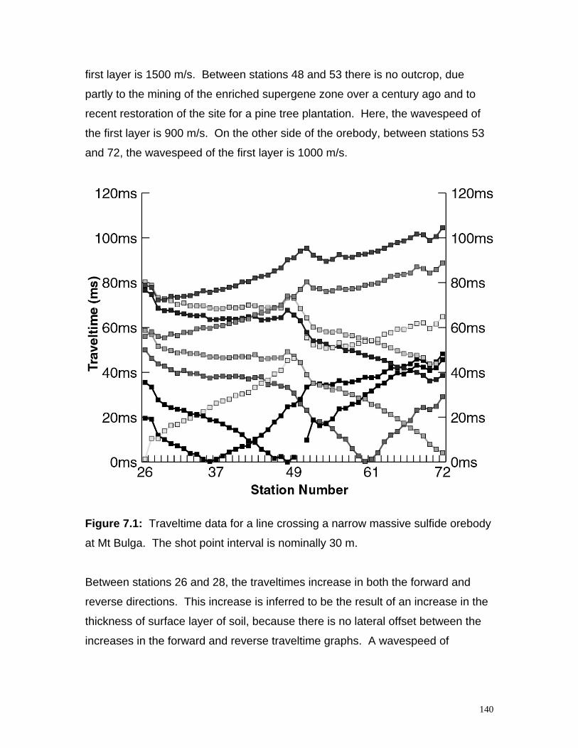
140
first layer is 1500 m/s. Between stations 48 and 53 there is no outcrop, due
partly to the mining of the enriched supergene zone over a century ago and to
recent restoration of the site for a pine tree plantation. Here, the wavespeed of
the first layer is 900 m/s. On the other side of the orebody, between stations 53
and 72, the wavespeed of the first layer is 1000 m/s.
Figure 7.1: Traveltime data for a line crossing a narrow massive sulfide orebody
at Mt Bulga. The shot point interval is nominally 30 m.
Between stations 26 and 28, the traveltimes increase in both the forward and
reverse directions. This increase is inferred to be the result of an increase in the
thickness of surface layer of soil, because there is no lateral offset between the
increases in the forward and reverse traveltime graphs. A wavespeed of
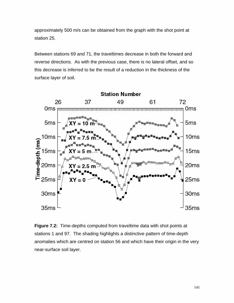
141
approximately 500 m/s can be obtained from the graph with the shot point at
station 25.
Between stations 69 and 71, the traveltimes decrease in both the forward and
reverse directions. As with the previous case, there is no lateral offset, and so
this decrease is inferred to be the result of a reduction in the thickness of the
surface layer of soil.
Figure 7.2: Time-depths computed from traveltime data with shot points at
stations 1 and 97. The shading highlights a distinctive pattern of time-depth
anomalies which are centred on station 56 and which have their origin in the very
near-surface soil layer.
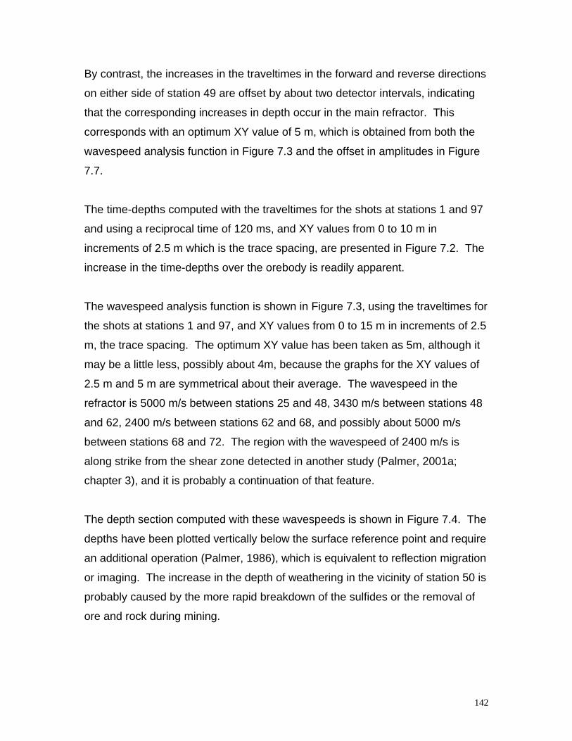
142
By contrast, the increases in the traveltimes in the forward and reverse directions
on either side of station 49 are offset by about two detector intervals, indicating
that the corresponding increases in depth occur in the main refractor. This
corresponds with an optimum XY value of 5 m, which is obtained from both the
wavespeed analysis function in Figure 7.3 and the offset in amplitudes in Figure
7.7.
The time-depths computed with the traveltimes for the shots at stations 1 and 97
and using a reciprocal time of 120 ms, and XY values from 0 to 10 m in
increments of 2.5 m which is the trace spacing, are presented in Figure 7.2. The
increase in the time-depths over the orebody is readily apparent.
The wavespeed analysis function is shown in Figure 7.3, using the traveltimes for
the shots at stations 1 and 97, and XY values from 0 to 15 m in increments of 2.5
m, the trace spacing. The optimum XY value has been taken as 5m, although it
may be a little less, possibly about 4m, because the graphs for the XY values of
2.5 m and 5 m are symmetrical about their average. The wavespeed in the
refractor is 5000 m/s between stations 25 and 48, 3430 m/s between stations 48
and 62, 2400 m/s between stations 62 and 68, and possibly about 5000 m/s
between stations 68 and 72. The region with the wavespeed of 2400 m/s is
along strike from the shear zone detected in another study (Palmer, 2001a;
chapter 3), and it is probably a continuation of that feature.
The depth section computed with these wavespeeds is shown in Figure 7.4. The
depths have been plotted vertically below the surface reference point and require
an additional operation (Palmer, 1986), which is equivalent to reflection migration
or imaging. The increase in the depth of weathering in the vicinity of station 50 is
probably caused by the more rapid breakdown of the sulfides or the removal of
ore and rock during mining.
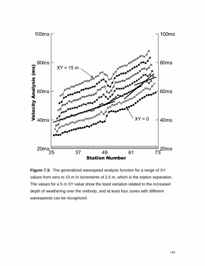
143
Figure 7.3: The generalized wavespeed analysis function for a range of XY
values from zero to 15 m in increments of 2.5 m, which is the station separation.
The values for a 5 m XY value show the least variation related to the increased
depth of weathering over the orebody, and at least four zones with different
wavespeeds can be recognized.
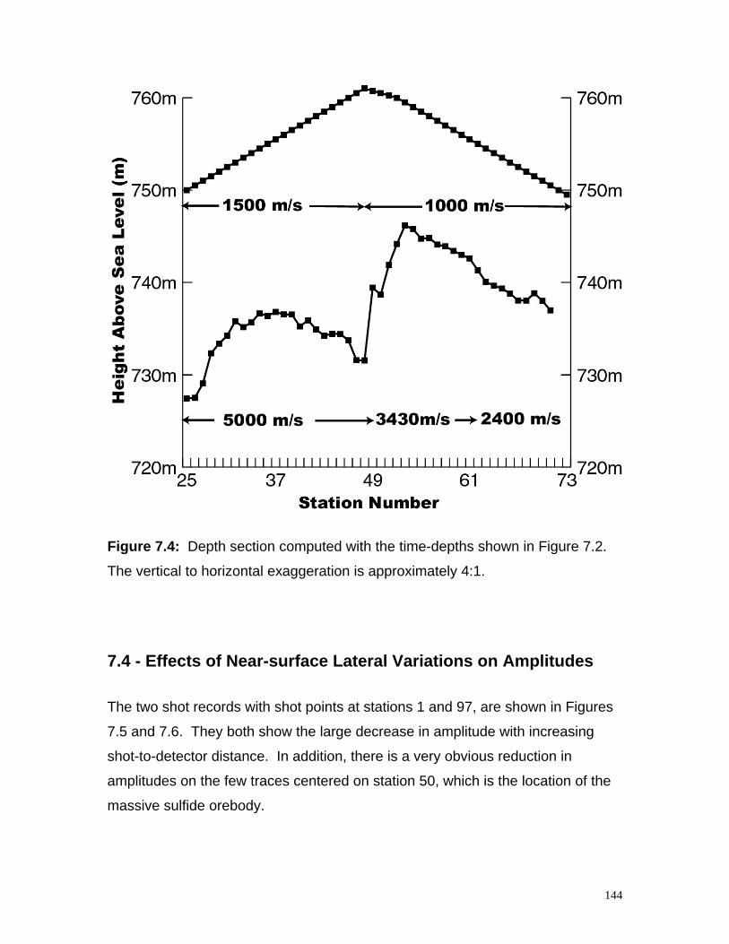
144
Figure 7.4: Depth section computed with the time-depths shown in Figure 7.2.
The vertical to horizontal exaggeration is approximately 4:1.
7.4 - Effects of Near-surface Lateral Variations on Amplitudes
The two shot records with shot points at stations 1 and 97, are shown in Figures
7.5 and 7.6. They both show the large decrease in amplitude with increasing
shot-to-detector distance. In addition, there is a very obvious reduction in
amplitudes on the few traces centered on station 50, which is the location of the
massive sulfide orebody.
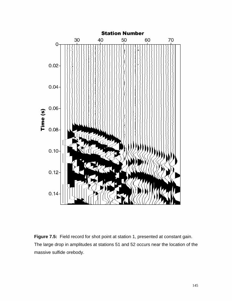
145
Figure 7.5: Field record for shot point at station 1, presented at constant gain.
The large drop in amplitudes at stations 51 and 52 occurs near the location of the
massive sulfide orebody.
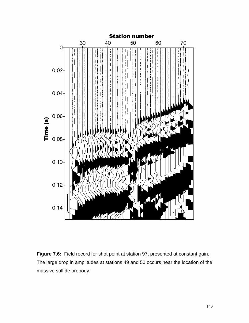
146
Figure 7.6: Field record for shot point at station 97, presented at constant gain.
The large drop in amplitudes at stations 49 and 50 occurs near the location of the
massive sulfide orebody.
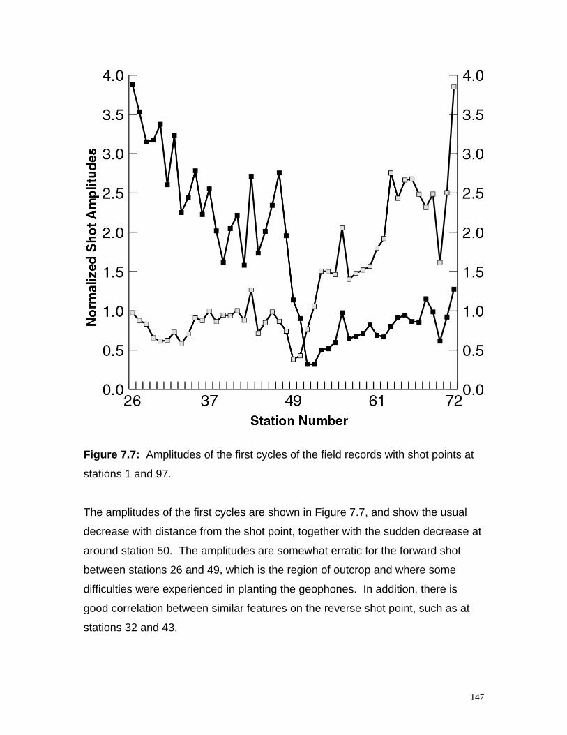
147
Figure 7.7: Amplitudes of the first cycles of the field records with shot points at
stations 1 and 97.
The amplitudes of the first cycles are shown in Figure 7.7, and show the usual
decrease with distance from the shot point, together with the sudden decrease at
around station 50. The amplitudes are somewhat erratic for the forward shot
between stations 26 and 49, which is the region of outcrop and where some
difficulties were experienced in planting the geophones. In addition, there is
good correlation between similar features on the reverse shot point, such as at
stations 32 and 43.
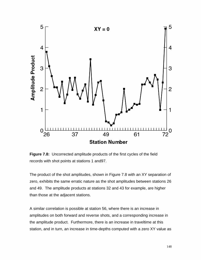
148
Figure 7.8: Uncorrected amplitude products of the first cycles of the field
records with shot points at stations 1 and97.
The product of the shot amplitudes, shown in Figure 7.8 with an XY separation of
zero, exhibits the same erratic nature as the shot amplitudes between stations 26
and 49. The amplitude products at stations 32 and 43 for example, are higher
than those at the adjacent stations.
A similar correlation is possible at station 56, where there is an increase in
amplitudes on both forward and reverse shots, and a corresponding increase in
the amplitude product. Furthermore, there is an increase in traveltime at this
station, and in turn, an increase in time-depths computed with a zero XY value as
149
shown in Figure 7.2. An examination of Figure 7.1, shows that the increase in
the traveltime occurs at the same geophone location for both the forward and
reverse shots, that is, there is no lateral displacement. Therefore, the increase in
depth occurs in the surface soil layer, rather than in the main refractor. The near-
surface origin is also supported by the characteristic pattern produced the time-
depths with in Figure 7.2 (Palmer, 1986, p107-111).
These results indicate that the occurrence of the soil surface layer produces
increases in seismic amplitudes. This is clearly indicated at station 56, as well as
at stations 32, 35, 41 and 43. In the latter cases, the time-depth anomalies are
not as large, but nevertheless, they are consistent with the hypothesis.
The hypothesis is further supported by the large increase in the surface soil layer
at stations 26 and 27 which corresponds with an increase in amplitudes, as well
as the decrease in the surface layer at stations 70 and 71, which correlates with
a decrease in amplitudes.
The variations in amplitudes with varying surface layers can be explained with
the transmission coefficients of the Zoeppritz equations, viz.:
Trans Coeff = 2 v lower ρ lower / (v lower ρ lower + v upper ρ upper) (7.1)
where
v upper is the wavespeed in the upper or surface layer,
ρ upper is the density in the upper or surface layer,
v lower is the wavespeed in the lower layer, and
ρ lower is the density in the lower layer.
This form of the equation is a little different from the standard, because the signal
is travelling upwards from the refractor.
150
In general, v upper < v lower and ρ upper < ρ lower. Therefore, the transmission
coefficient in equation 7.1 will vary from one, that is, there is no surface soil layer,
to two, that is, the surface soil layer wavespeed and density are much less than
those of the layer below. In those cases where there is a surface soil layer, there
will be an increase in amplitudes, because the transmission coefficient will
usually be greater than one.
The wavespeeds and densities in the upper soil layer can vary over quite large
ranges. Furthermore, it can be difficult to accurately map any rapid lateral
variations with for example, seismic methods. Therefore, it may not always be
possible to conveniently derive correction factors based on the Zoeppritz
equation.
In such situations where there is significant variation in the surface soil layer, it is
suggested that the minimum values, rather than the average values, be taken as
representative of that region. For example, the amplitude product for the region
between stations 30 and 48 will be taken as about 1.3, rather than the average of
about 2 or the maximum of about 2.5.
However, a wavespeed of approximately 500 m/s can be recovered for the
surface soil layer between stations 26 and 28. If the densities are ignored, then
the transmission coefficient computed with equation 7.1, is 1.5. Since the
amplitudes are multiplied in Figure 7.8, the transmission coefficient must be
squared, prior to application. The squared correction factor of 2.25 satisfactorily
accounts for the increase in amplitude, as shown in Table 1.
151
7.5 - Relationships Between Amplitudes and RefractorWavespeeds
The normalized amplitude products are shown in Figure 7.9 for XY values from
zero to 10 m. The values shown include the addition of a constant, namely, 1 for
an XY value of 2.5 m, 2 for an XY value of 5 m, and so on, in order to separate
the graphs.
The anomalous amplitude product at station 56 is readily seen on the graph for
the zero XY value. As the XY value is systematically increased, the forward and
reverse amplitude anomalies are separated, with the result that the anomalous
product separates into two, which correspond with the forward and reverse shot
amplitude values. The forward amplitude systematically moves to the right, while
the reverse value moves to the left. The pattern is similar to that produced by
traveltime anomalies which originate in the near-surface (Palmer, 1986, p107-
111), as shown in Figure 7.2 for station 56.
This pattern with the amplitude products which can be seen clearly at station 56,
can also be recognized with some difficulty between stations 27 and 48.
Figure 7.7 shows that the very low amplitudes associated with the massive
sulfides, occur at stations 51 and 52 on the forward shot and 49 and 50 on the
reverse shot. The amplitude products in Figure 7.9, show that this interval is a
minimum for an XY value of 5 m, and that it occurs at stations 50 and 51. For
other XY values, this zone is wider.
The accompanying table summarizes the amplitude products and the correlation
with wavespeeds. In general, the agreement is good.
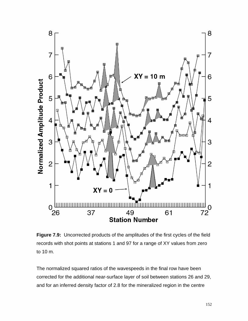
152
Figure 7.9: Uncorrected products of the amplitudes of the first cycles of the field
records with shot points at stations 1 and 97 for a range of XY values from zero
to 10 m.
The normalized squared ratios of the wavespeeds in the final row have been
corrected for the additional near-surface layer of soil between stations 26 and 29,
and for an inferred density factor of 2.8 for the mineralized region in the centre
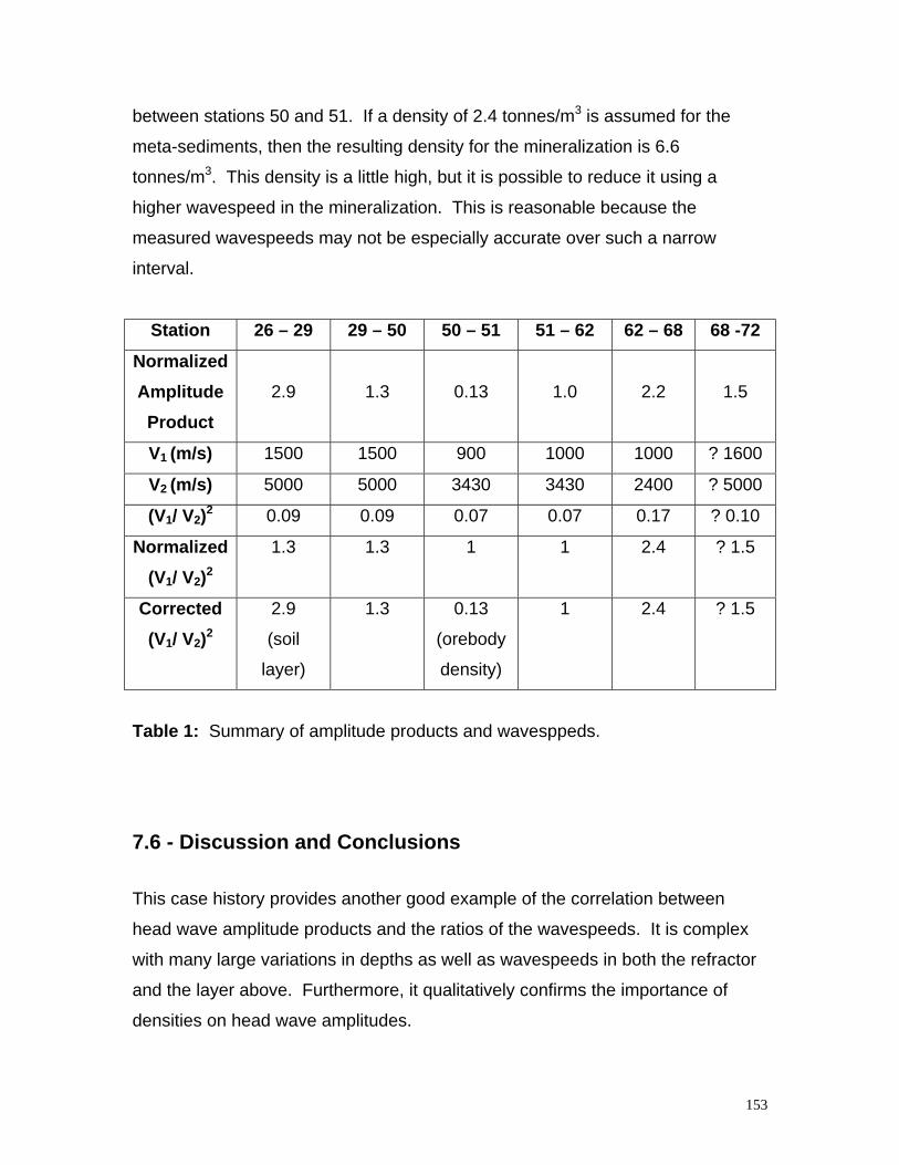
153
between stations 50 and 51. If a density of 2.4 tonnes/m3 is assumed for the
meta-sediments, then the resulting density for the mineralization is 6.6
tonnes/m3. This density is a little high, but it is possible to reduce it using a
higher wavespeed in the mineralization. This is reasonable because the
measured wavespeeds may not be especially accurate over such a narrow
interval.
Station 26 – 29 29 – 50 50 – 51 51 – 62 62 – 68 68 -72NormalizedAmplitudeProduct
2.9 1.3 0.13 1.0 2.2 1.5
V1 (m/s) 1500 1500 900 1000 1000 ? 1600
V2 (m/s) 5000 5000 3430 3430 2400 ? 5000
(V1/ V2)2 0.09 0.09 0.07 0.07 0.17 ? 0.10
Normalized(V1/ V2)2
1.3 1.3 1 1 2.4 ? 1.5
Corrected(V1/ V2)2
2.9
(soil
layer)
1.3 0.13
(orebody
density)
1 2.4 ? 1.5
Table 1: Summary of amplitude products and wavesppeds.
7.6 - Discussion and Conclusions
This case history provides another good example of the correlation between
head wave amplitude products and the ratios of the wavespeeds. It is complex
with many large variations in depths as well as wavespeeds in both the refractor
and the layer above. Furthermore, it qualitatively confirms the importance of
densities on head wave amplitudes.
154
The case history also provides a valuable insight into the importance of near-
surface variations and geophone coupling on the measured refraction
amplitudes.
Between stations 50 and 72 where there is no outcrop, the amplitudes and the
amplitude products are essentially a function of the wavespeeds in the refractor
and the layer above. However, at station 56, there is an increase in amplitudes
which correlates with an increase in traveltimes and time-depths. These results
indicate that the amplitude variation is related to the near-surface layering, rather
than to the coupling of the geophones with the ground.
The results for the region between stations 26 and 50, where there was
extensive outcrop, support this interpretation, because all of the amplitude
anomalies can be associated with traveltime anomalies.
The presentation of both amplitude products and time-depths for a range of XY
values from zero to more than the optimum value, provides a convenient and
effective method for recognizing near-surface anomalous zones of limited lateral
extent.
The increases in amplitudes are compatible with the transmission coefficients of
the Zoeppritz equations. As the seismic signal approaches the surface from the
refractor, there is an increase in seismic amplitude where there is another layer
with lower wavespeed and or density.
In general, this change in amplitude can be ignored when there are several
continuous layers above the refractor, because the same increase in amplitudes
occurs at each detector. In these situations, the amplitudes are adequately
described with the head coefficients, together with a geometric spreading factor.
155
Where there are lateral changes in the surface layers, such as the irregular
development of a surface soil layer, there can be large variations in amplitudes
by a factor of between 1 and 2. If these layers have sufficient lateral extent so
that they can be mapped, such as the region between stations 26 and 28, then
an approximate correction factor can be computed with the transmission
coefficients of the Zoeppritz equations.
However, this is not always possible. Under these circumstances, the minimum
amplitudes are probably the most representative.
7.7 - References
Bycroft, G. N., 1956, Forced vibrations of a rigid plate on a semi-infinite elastic
space: Roy. Soc. London, 248, 327-368.
Fail, J. P., Grau, G., and Lavergne, M., 1962, Couplage des sismographes avec
le sol: Geophys. Prosp., 10, 128-147.
Lamer, A., 1970, Couplage sol-geophone: Geophys. Prosp., 18, 300-319.
Palmer, D., 1980, The generalized reciprocal method of seismic refraction
interpretation: Society of Exploration Geophysicists.
Palmer, D., 1986, Refraction seismics - the lateral resolution of structure and
seismic: Geophysical Press.
Palmer, D., 2001a, Imaging refractors with the convolution section: Geophysics
66, 1582-1589.
156
Palmer, D., 2001b, Resolving refractor ambiguities with amplitudes: Geophysics
66, 1590-1593.
Pieuchot, M., 1984, Seismic instrumentation: Geophysical Press.
Polak, E. J., 1969, Attenuation of seismic energy and its relation to the properties
of rocks: Ph D thesis, University of Melbourne, p4.7-4.9.
157
Chapter 8
Enhancement of Later Events in theRCS with Dip Filtering
8.1 - Summary
Later events, which occur in the shot records, are also treated in the same
manner as first events with the convolution process. Both the addition of the
traveltimes and the multiplication of amplitudes take place. However, there can
be additional features in which cross-convolution artifacts are also generated.
These artifacts which are formed by the convolution of events from different
refractors, occur as relatively steeply dipping events in the refraction convolution
section (RCS) and therefore, they can be removed by dip filtering. The filtered
RCS shows better continuity of events than is the case with the unfiltered
section.
For events which have traveled through the surface layer, the filtered RCS shows
a series of events which occur at a time which is a function of the distance
between the two shot points and the wavespeed in the surface layer. The time of
this event can be used to improve the estimates of the wavespeed in the surface
layer.
158
8.2 - Introduction
The generation of the refraction convolution section (RCS) (Palmer, 2000)
produces a set of traces with the superficial appearance of a seismic reflection
section. It has been demonstrated that the RCS reproduces the time structure of
the refractor interface with first arrivals, while the amplitudes which are largely
corrected for geometric spreading, are essentially a function of the square of the
head coefficient. It has also been demonstrated that the head coefficient is given
approximately by the ratio of the wavespeeds in the upper layer and refractor.
The RCS amplitudes can be employed to image the refractor, to resolve some of
the ambiguities in the determination of wavespeeds in the refractor, and to obtain
a measure of azimuthal anisotropy with three dimensional methods.
To date, research has focused primarily on the portion of the RCS which
corresponds with the first arrivals, and little attention has been directed at later
events. However, the convolution process performs the same operations on later
arrivals as it does with the first events. These operations are the addition of the
traveltimes in the forward and reverse directions, which replaces of moveout from
trace to trace with a constant amount equal to the reciprocal time, the time from
the forward shot point to the reverse shot point, and the multiplication of the
amplitudes. The addition of the traveltimes produces the relative time structure
on the refracting interface, while the amplitude product effectively compensates
for the large geometric spreading which is characteristic of refraction data. The
true time structure on the interface can be obtained by subtracting the reciprocal
time. As the reciprocal time generally decreases with deeper layers, the
shallower layers occur at later times in the RCS.
One feature of the RCS is the generation of what will be termed cross-
convolution events with later arrivals. In this case, the convolution operation
adds arrivals from different refractors, and therefore generates artifacts which
have no geophysical significance. For example, it is possible to produce an
159
event which is the addition of the traveltimes from the refractor in the forward
direction, with the traveltimes from the surface layer in the reverse direction. In
practice, these artifacts occur as pairs, that is there is also an event produced by
the addition of the traveltimes from the surface layer in the forward direction, with
the traveltimes from the refractor in the reverse direction. Because of the
different moveouts or wavespeeds, these events appear as relatively steeply
dipping features in the RCS.
This study describes the use of dip filtering in the f-k domain (Sheriff and Geldart,
1995), to remove the cross-convolution events, with the aim of enhancing those
later events which may have geological significance.
8.3 - Generation of Useful Events and Artifacts in the RCS
The generation of useful later events in the RCS can best be demonstrated with
the ground-coupled air wave. While it is recognized that the imaging of the air
wave has minimal geological significance, it is employed in this study because its
high amplitude improves its clarity in the RCS.
Figure 8.1 is a shot record from a shallow seismic refraction survey at Mt Bulga,
which has been described previously (Palmer, 2001). The record shows the first
arrivals between about 70 ms and 130 ms as very low amplitude signals, and a
very high amplitude event between 350 ms and 1000 ms. The first arrivals are
refracted from the base of the weathering, while the second arrivals are the
ground-coupled air wave.
Figure 8.2 shows the shot record in the reverse direction. The same two events
can be clearly identified, but in this case, the relative amplitude of the ground-
coupled air wave is lower.
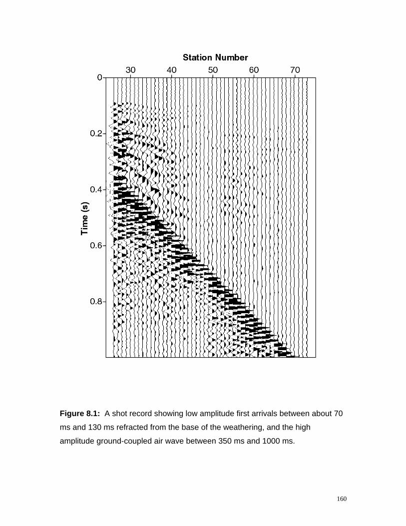
160
Figure 8.1: A shot record showing low amplitude first arrivals between about 70
ms and 130 ms refracted from the base of the weathering, and the high
amplitude ground-coupled air wave between 350 ms and 1000 ms.
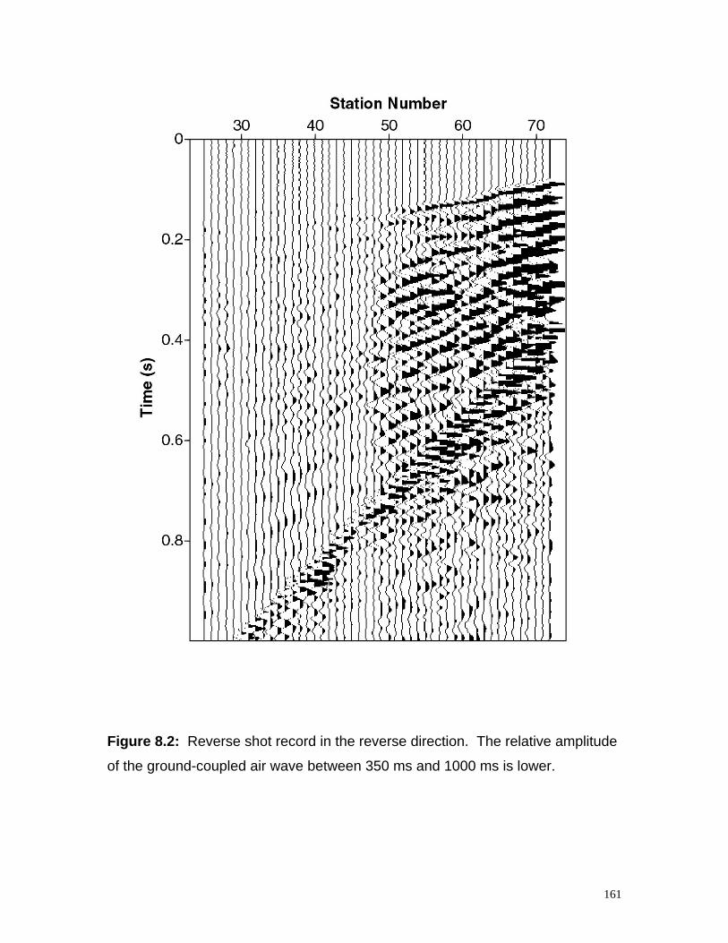
161
Figure 8.2: Reverse shot record in the reverse direction. The relative amplitude
of the ground-coupled air wave between 350 ms and 1000 ms is lower.
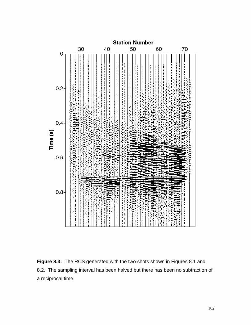
162
Figure 8.3: The RCS generated with the two shots shown in Figures 8.1 and
8.2. The sampling interval has been halved but there has been no subtraction of
a reciprocal time.
163
The RCS generated with these two shots is shown in Figure 8.3. The sampling
interval has been halved (Palmer, 2001), but there has been no subtraction of a
reciprocal time. The presentation gain is low so that the portion of the RCS
which corresponds with the convolved events from the refractor around 150 ms,
becomes essentially featureless. However, the gain facilitates the recognition of
the strong event at approximately 700 ms between stations 29 and 68. The
limited lateral extent of this event occurs because the recording time of one
second was insufficient to record the air wave at the distant detectors.
In addition, the presentation gain highlights the cross-convolution events which
start a few traces from the left side of the section at 300 ms and continue to
about 550 ms near the right side of the section. The recognition of the
companion artifact which starts on the right hand side and finishes on the left is
not as clearly evident in Figure 8.3 and requires more careful inspection.
8.4 - Removal of Cross-convolution Artifacts with Dip Filtering
The transformation of the in RCS in Figure 8.3 from the time-distance domain to
the frequency-wavenumber (fk) domain with the double Fourier transform, is
shown in Figure 8.4. It shows signal centered on the frequency axis, which
corresponds with the horizontal events, and signal spread out parallel to the
wavenumber axis, which is inferred to correspond with the cross-convolution
events.
Figure 8.6 shows the fk domain after the application of a filter to remove all signal
other than that centered on the frequency axis, while Figure 8.5 shows the RCS
after the application of the filter. The event which corresponds with the time-
depth of the ground-coupled air wave can be clearly seen at about 0.710 s.
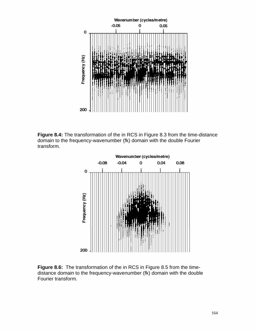
164
Figure 8.4: The transformation of the in RCS in Figure 8.3 from the time-distancedomain to the frequency-wavenumber (fk) domain with the double Fouriertransform.
Figure 8.6: The transformation of the in RCS in Figure 8.5 from the time-distance domain to the frequency-wavenumber (fk) domain with the doubleFourier transform.
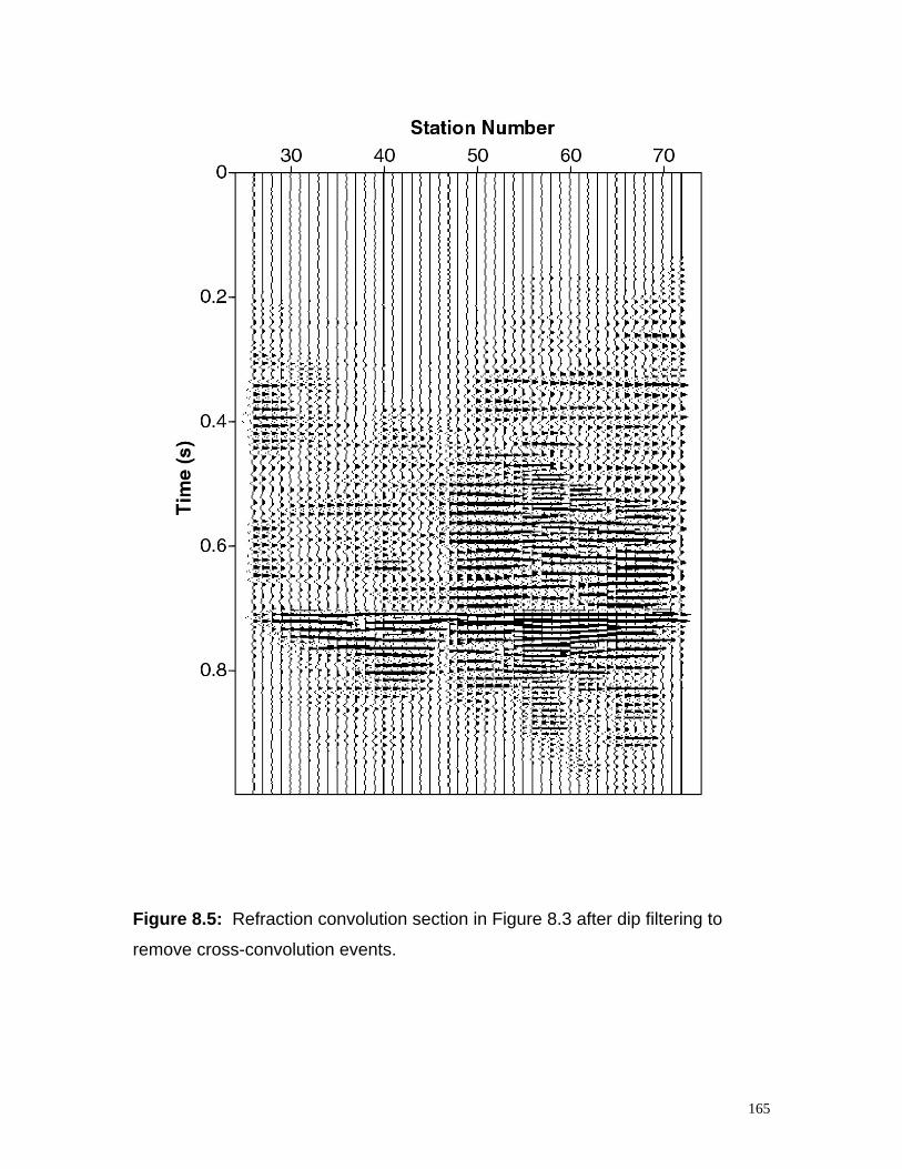
165
Figure 8.5: Refraction convolution section in Figure 8.3 after dip filtering to
remove cross-convolution events.
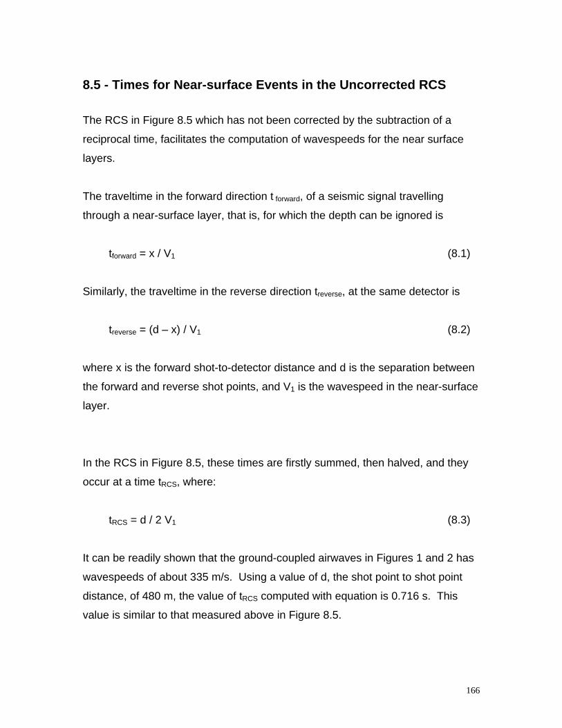
166
8.5 - Times for Near-surface Events in the Uncorrected RCS
The RCS in Figure 8.5 which has not been corrected by the subtraction of a
reciprocal time, facilitates the computation of wavespeeds for the near surface
layers.
The traveltime in the forward direction t forward, of a seismic signal travelling
through a near-surface layer, that is, for which the depth can be ignored is
tforward = x / V1 (8.1)
Similarly, the traveltime in the reverse direction treverse, at the same detector is
treverse = (d – x) / V1 (8.2)
where x is the forward shot-to-detector distance and d is the separation between
the forward and reverse shot points, and V1 is the wavespeed in the near-surface
layer.
In the RCS in Figure 8.5, these times are firstly summed, then halved, and they
occur at a time tRCS, where:
tRCS = d / 2 V1 (8.3)
It can be readily shown that the ground-coupled airwaves in Figures 1 and 2 has
wavespeeds of about 335 m/s. Using a value of d, the shot point to shot point
distance, of 480 m, the value of tRCS computed with equation is 0.716 s. This
value is similar to that measured above in Figure 8.5.
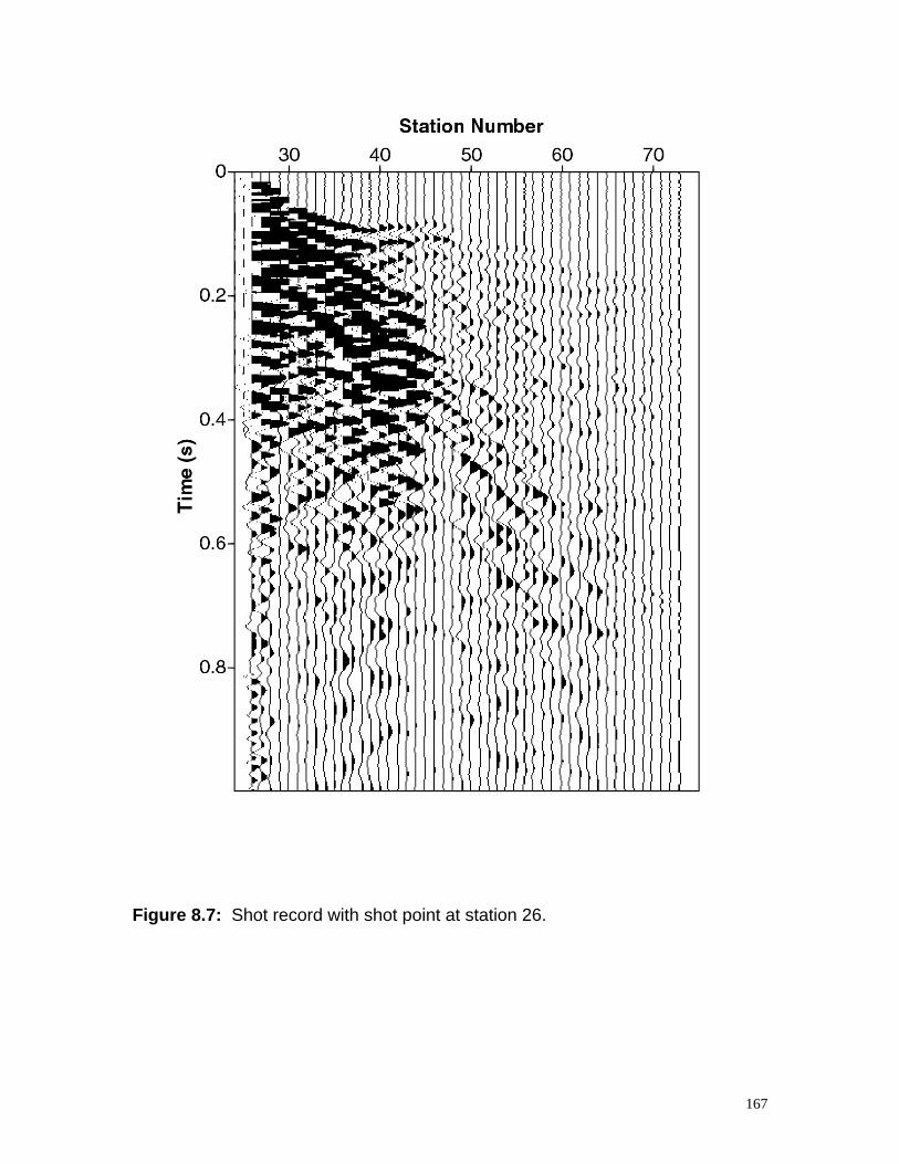
167
Figure 8.7: Shot record with shot point at station 26.
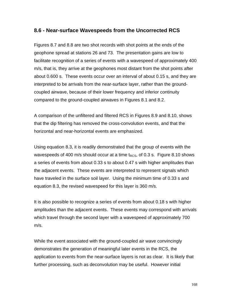
168
8.6 - Near-surface Wavespeeds from the Uncorrected RCS
Figures 8.7 and 8.8 are two shot records with shot points at the ends of the
geophone spread at stations 26 and 73. The presentation gains are low to
facilitate recognition of a series of events with a wavespeed of approximately 400
m/s, that is, they arrive at the geophones most distant from the shot points after
about 0.600 s. These events occur over an interval of about 0.15 s, and they are
interpreted to be arrivals from the near-surface layer, rather than the ground-
coupled airwave, because of their lower frequency and inferior continuity
compared to the ground-coupled airwaves in Figures 8.1 and 8.2.
A comparison of the unfiltered and filtered RCS in Figures 8.9 and 8.10, shows
that the dip filtering has removed the cross-convolution events, and that the
horizontal and near-horizontal events are emphasized.
Using equation 8.3, it is readily demonstrated that the group of events with the
wavespeeds of 400 m/s should occur at a time tRCS, of 0.3 s. Figure 8.10 shows
a series of events from about 0.33 s to about 0.47 s with higher amplitudes than
the adjacent events. These events are interpreted to represent signals which
have traveled in the surface soil layer. Using the minimum time of 0.33 s and
equation 8.3, the revised wavespeed for this layer is 360 m/s.
It is also possible to recognize a series of events from about 0.18 s with higher
amplitudes than the adjacent events. These events may correspond with arrivals
which travel through the second layer with a wavespeed of approximately 700
m/s.
While the event associated with the ground-coupled air wave convincingly
demonstrates the generation of meaningful later events in the RCS, the
application to events from the near-surface layers is not as clear. It is likely that
further processing, such as deconvolution may be useful. However initial
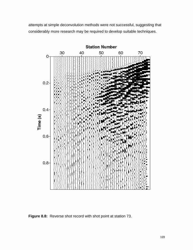
169
attempts at simple deconvolution methods were not successful, suggesting that
considerably more research may be required to develop suitable techniques.
Figure 8.8: Reverse shot record with shot point at station 73.
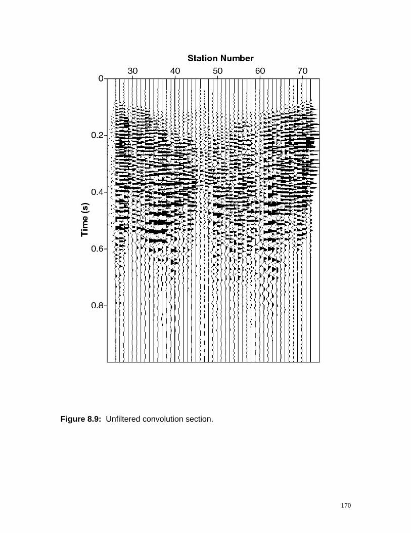
170
Figure 8.9: Unfiltered convolution section.
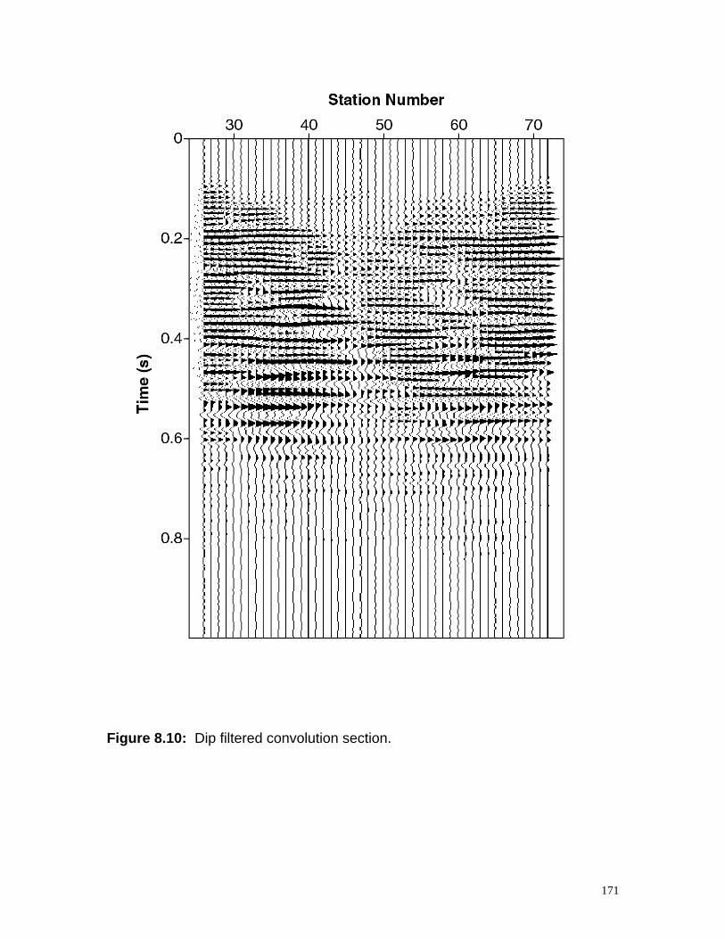
171
Figure 8.10: Dip filtered convolution section.
172
8.7 - Conclusions
Later events, which occur in the shot records, are also treated in the same
manner as first events with the convolution process. Both the addition of the
traveltimes and the multiplication of amplitudes take place. However, there is an
additional feature in which cross-convolution artifacts are also generated. These
artifacts occur as relatively steeply dipping events in the RCS and therefore, they
can be removed by dip filtering. The filtered RCS shows better continuity of
events than is the case with the unfiltered section.
For events which have traveled through the surface layer, the filtered RCS shows
a series of events which occur at a time which is a function of the distance
between the two shot points and the wavespeed in the surface layer. The time of
this event can be used to improve the estimates of the wavespeed in the surface
layer.
8.8 - References
Palmer, D., 2001, Imaging refractors with the convolution section: Geophysics
66, 1582-1589.
Sheriff, R. E., and Geldart, L. P., 1995, Exploration Seismology, 2nd edition:
Cambridge University Press.
173
Chapter 9
Stacking Seismic Refraction Data inthe Convolution Section
9.1 - Summary
The refraction convolution section (RCS) is an effective domain to vertically stack
shallow seismic refraction data, in order to improve signal-to-noise ratios (S/N).
The convolution operation essentially compensates for the effects of geometrical
spreading, and generates traces with much the same S/N ratios. Such traces
are optimum for stacking, unlike the traces on the original shot records.
A major benefit of stacking in the RCS domain is that it takes places before the
measurement of times or amplitudes. With other approaches which do not
routinely employ stacking, such as tomography, any variations in data quality are
addressed with the application of statistical methods to the traveltimes
determined on the original field data.
An essential requirement for stacking in the RCS domain are data which have
been acquired with a continuous roll along approach typical of reflection
methods, rather than with the more common static spread. Such operations are
more efficient and produce more data from the critical near-surface layers, but
they would require significant re-capitalization of most shallow seismic field
operations.

174
9.2 - Introduction
It is well known that the source energy requirements for seismic refraction
surveys are considerably greater than those for seismic reflection surveys for the
same target. The maximum source-to-detector distance for seismic reflection
surveys is generally less than the target depth, whereas the minimum source-to-
detector distance with refraction surveys is usually greater than four times the
target depth. In addition, the geometric spreading component is the reciprocal of
the distance traveled for reflected signals, while the corresponding function for
refracted signals is the reciprocal of the distance squared. Both the longer path
lengths and the more rapid spreading factors result in low refraction amplitudes
and therefore higher source energy requirements. Commonly, the refraction
source is more than ten times the size of the reflection source for the same
target.
Explosives are the standard energy source in most shallow seismic refraction
surveys, and adequate signal-to-noise (S/N) ratios are readily achieved by
increasing the size of the charge. However, this is not always practical in many
environmentally sensitive or urban areas, and it normally results in either poor
quality data due to insufficient charge sizes, or more commonly, no acquisition of
data at all.
In some cases, it is possible to use vertical signal stacking with repetitive
sources, such as hammers and dropping weights. Nevertheless, this approach
can be of limited usefulness, because many repetitions can be required to obtain
reasonable S/N ratios, especially where urbanization is the major source of
noise.
In addition, vertical stacking can result in slow rates of progress where there are
many source points. Walker et al, (1991) demonstrate that one of the most
important factors in improving the reliability of shallow seismic refraction
175
interpretation is a detailed mapping of the wavespeeds in the layers above the
target refractor using a high density of source points. It is not uncommon to
employ a source point between every other pair of geophones.
This study demonstrates the use of vertical stacking with a CMP-like method
using the refraction convolution section (RCS). Redundant or multi-fold
refraction data are acquired with a continuous roll along approach, which is
standard with reflection acquisition. Multiple overlapping RCS are generated with
pairs of shots with the same shot point to shot point separation. The ensemble of
RCS are then sorted and gathered, in much the same way as reflection shot
records, and the gathers are then stacked.
The RCS is a suitable domain in which to stack refraction data when the shot
size, depth and separation are uniform, because the events have approximately
the same S/N ratios. With effective vertical stacking, the S/N ratio improves as
the square root of the number of traces in the stack, but only when the S/N ratios
of the original traces are much the same. Excessively noisy traces, that is traces
with an anomalously low S/N ratio, can significantly degrade the stack and
reduce the benefits of stacking. This situation occurs with stacking refraction
shot records, because there can be large variations in S/N ratios related to the
effects of geometric spreading. Traces at a given station with nearby source
points will have high S/N ratios while traces at the same station with more distant
source points will have lower S/N ratios. The large range in S/N ratios with
refraction shot records significantly reduces the effectiveness of stacking traces
from various shot records with a surface consistent approach.
Shearer (1991) demonstrates stacking shot records in which the shot-receiver
distance is preserved, but not the individual station locations, in order to improve
S/N ratios with earthquake data (see also Lay and Wallace, 1995, p215-216).
However, this approach is not a viable option with shallow refraction data,
176
because it does not accommodate lateral variations in either the depths to or
wavespeeds in the target refractor.
A major advantage of stacking in the RCS domain is that S/N ratios can be
enhanced prior to the measurement of parameters, such as times or amplitudes.
By contrast, tomographic methods measure traveltimes from the shot records
which have varying S/N ratios, and then seek to minimize any errors with a
statistical approach.
9.3 – The Cobar Stacked RCS Section
High resolution data were recorded with a 48 trace recorder, and single 40 Hz
geophones with a 10 m spacing, as part of a regional seismic reflection survey
(Drummond et al, 1992) across the Cobar Basin (Glen et al, 1994), in the central
west of NSW, Australia. The aim of these high resolution lines was to image the
near surface layers, which in these areas were dipping predominantly in the
vertical direction. The seismic source was a 10 kg charge of a high velocity
seismic explosives at a depth of 40 m, and the shot point interval was 30 m.
The data were recorded with off-end shots in both the forward and reverse
directions in order the obtain large shot-to-detector distances for the vertically
dipping reflection targets. For example, the first shot was at station 96, and the
geophones were from station 95 to station 48. The next shot was at station 90
and the geophones from station 89 to 42, a shift of 60 m. Subsequent shots
continued through to station 48 with geophones between stations 47 and 0. The
geophone array then remained static while the shot points at 60 m intervals
within the array at stations 42, 36, etc., were recorded. The recording process
was then reversed. The shot point at station 3 was recorded with geophones
between stations 4 and 51. Subsequent shots were at 60 m intervals (stations 9,
15, etc.), and the geophone array was moved up by the same amount in each
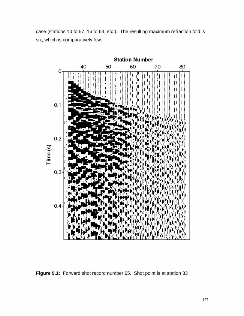
177
case (stations 10 to 57, 16 to 63, etc.). The resulting maximum refraction fold is
six, which is comparatively low.
Figure 9.1: Forward shot record number 65. Shot point is at station 33
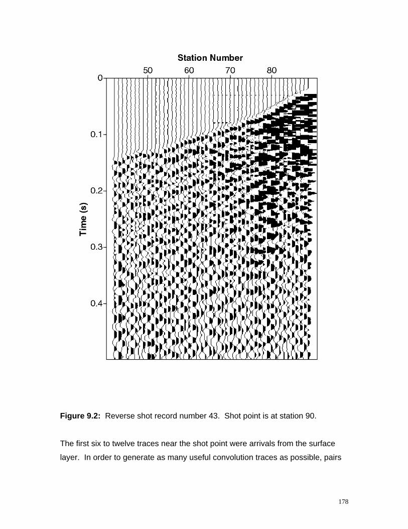
178
Figure 9.2: Reverse shot record number 43. Shot point is at station 90.
The first six to twelve traces near the shot point were arrivals from the surface
layer. In order to generate as many useful convolution traces as possible, pairs
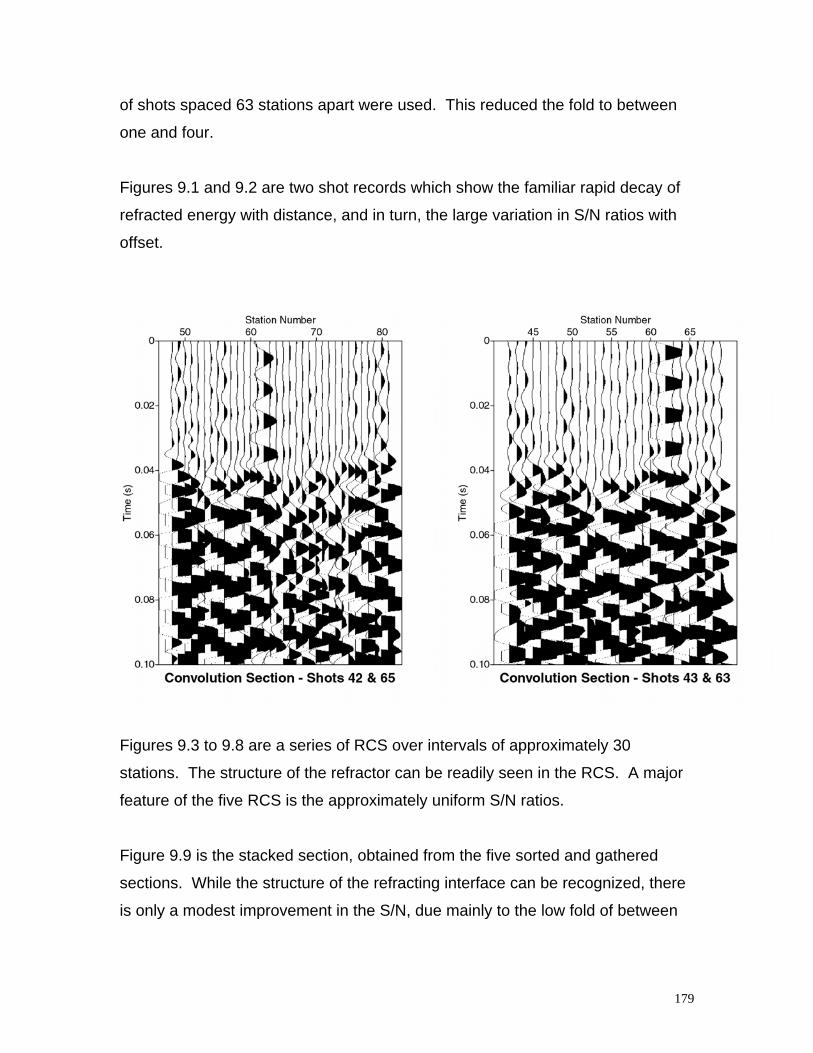
179
of shots spaced 63 stations apart were used. This reduced the fold to between
one and four.
Figures 9.1 and 9.2 are two shot records which show the familiar rapid decay of
refracted energy with distance, and in turn, the large variation in S/N ratios with
offset.
Figures 9.3 to 9.8 are a series of RCS over intervals of approximately 30
stations. The structure of the refractor can be readily seen in the RCS. A major
feature of the five RCS is the approximately uniform S/N ratios.
Figure 9.9 is the stacked section, obtained from the five sorted and gathered
sections. While the structure of the refracting interface can be recognized, there
is only a modest improvement in the S/N, due mainly to the low fold of between
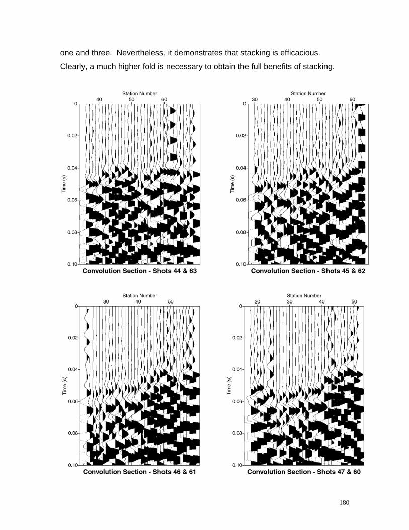
180
one and three. Nevertheless, it demonstrates that stacking is efficacious.
Clearly, a much higher fold is necessary to obtain the full benefits of stacking.
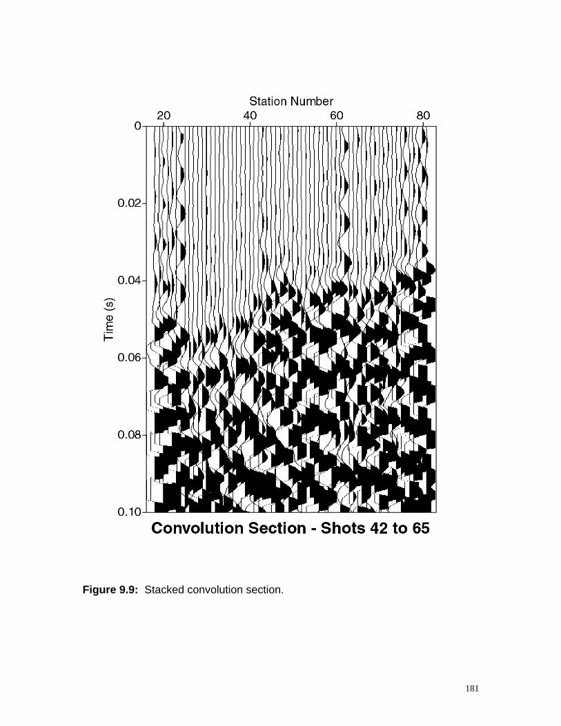
181
Figure 9.9: Stacked convolution section.
182
9.4 - The Static Geophone Spread
For the effective use of stacking, it is necessary to use RCS with relatively
uniform S/N ratios, and therefore to employ uniform acquisition parameters. The
relevant parameters are consistent charge size and depth, as well as a uniform
separation between the forward and reverse sources. Although these field
parameters are the norm with the refraction data acquired with routine reflection
surveys for petroleum and coal exploration and for regional reflection surveys in
fold belts, they are uncommon with most shallow seismic refraction surveys
carried out for geotechnical, groundwater and environmental applications.
The majority of shallow seismic refraction surveys carried out for geotechnical
and other shallow applications acquire data in discrete units or spreads. With
these surveys, a static spread of detectors is used with a multiplicity of source
points located at several offset positions on one side, through the spread and to
offset positions on the other side. The number of shot points recorded for each
spread has increased substantially in recent years in order to improve the
determination of the wavespeed stratification above the target refractor, and it is
now common to record more than eleven shots for a spread of 12 detectors
(Walker et al, 1991). For the typical survey length of 400 m for a road cutting,
approximately eight spreads of 12 detectors with a 2 detector overlap are
required (Walker et al, 1991), making a total of 88 shot points.
However, it is questionable whether even this considerable number of shot points
achieves the stated objectives of defining the wavespeed stratification within the
weathered layer. An inspection of published data (Walker et al, 1991, Fig. 6),
shows that the vast majority of the traveltime data (~ 90%) are arrivals refracted
from the base of the weathering. Although it is essential to ensure some
redundancy in the traveltime data in order to resolve the fundamental ambiguity
of determining the number of layers detected (Palmer, 1986, p21-29; Lankston,
1992), the majority of the data from the main refractor are generally not used in
183
the subsequent data processing stages. It questions the fundamental
effectiveness of the static spread approach to acquiring shallow seismic
refraction data.
There are also concerns about the efficiency of field operations with static
spreads. There can be a comparatively large number of shot points per unit
distance because of the occupation of many shot point locations on two and
often three occasions, as well as the common practice of using an overlap of
several detectors. The repeated occupation of shot points can be
environmentally damaging as well as time consuming. Furthermore, field
operations do not progress smoothly, because the acquisition of data ceases
while the spread of detectors is retrieved and then re-deployed for the next
adjacent spread.
The static spread approach also results in a wide range of source energy
requirements for the different offsets and the different layers above the target.
Relatively low source energies are required for signals propagating in the shallow
near-surface layers, while considerably greater source energies are required for
the deeper target refractors. Since the majority of traveltimes are from the main
refractor, there can be a large source energy requirement. As mentioned
previously, many of these times are not used in the data processing, which
suggests that more efficient approaches may be possible.
This study proposes the continuous acquisition of shallow seismic refraction data
be employed routinely for geotechnical, groundwater and environmental
applications.
9.5- Continuous Acquisition of Shallow Seismic Refraction Data
Continuous acquisition of redundant or multi-fold data is the norm with seismic
reflection methods. With this technique, the source point maintains a fixed
184
position in relation to the detector spread, which for land operations is usually a
split spread with the source in the centre of the detectors. The constant
geometry is obtained by laying out more detectors than there are channels in the
recording instruments and then selecting the required channels with a roll along
switch. Continuous and efficient operations are achieved with a single pass of
the seismic source along the line in conjunction with the continual removal of
detectors from the start of the line after they are no longer required, and their
placement at the other end to which the source is progressing.
Better and more uniform coverage of all refractors commonly occurs.
Roll along acquisition methods can provide better data for either the conventional
or convolution approaches where two or more adjacent static spreads would
normally be employed. Comparisons of field operations show that in fact, there
can be a reduction in the number of shot points per unit distance of coverage.
For example, for a 400 m long survey for a road cutting using a 15 m shot
spacing and a 5 m detector interval, a total of only about 55 shots would be
required. A 12 channel seismic recorder would not be suitable for roll along
operations, because the maximum shot to detector distance of 30 m would
generally be insufficient to record enough arrivals from the base of the
weathering. However, a 24 channel seismic recorder, which is widely used in
shallow refraction surveys, would be suitable, and in many cases might even
permit a reduction in the trace spacing to 3m to further improve the resolution of
the wavespeed stratification in the weathered layer. A 48 channel system would
provide further improvements in data quality through additional reductions in
trace spacing, as well as enhanced capabilities with swath or partial three
dimensional profiling.
The comparatively large number of shot points per unit distance with adjacent
static spreads is a result of the occupation of shot point locations on two and
often three occasions, as well as the common practice of using an overlap of
185
several detectors. In contrast, the continuous recording of refraction data with
the roll along method involves the once-only occupation of each source point,
and incorporates a uniform overlap as an integral part of the method.
Accordingly, it represents a more efficient use of equipment and field personnel
with a lower environmental impact.
For surveys in which only limited coverage is required, it is still desirable to
replace the single static spread with a quasi roll along approach. However, the
number of source points may in fact increase with this approach, in order to
obtain sufficient data redundancy for stacking.
9.6 – Determination of Fold with RCS Data
The maximum fold obtained with continuous refraction acquisition using a split
spread shooting method is similar to that obtained with reflection data, viz.
Maximum fold = Number of detectors / (Shot spacing x 2) (9.1)
Note that the shot spacing is given as the number of detector intervals.
The validity of equation 9.1 can be demonstrated with a simple example.
Suppose that the recording system has 48 channels, the shot is at station 25 and
that the live geophones are from stations 1 to 24 and 26 to 49. For the same
split spread recording pattern, reversed shots at stations 1 and 49, which
represent a shot spacing of 24 stations, are the minimum necessary to compute
a time-depth at each detector, provided all arrivals are from the target refractor.
The maximum resulting fold is therefore one.
186
At the other extreme, if the shot spacing is reduced to a single detector interval,
then the maximum fold is 24. For the more common shot spacing of two detector
intervals, the maximum fold is 12.
In general, not all detectors will record arrivals from the target refractor. Suppose
that the first six arrivals on either side of the shot point are from layers other than
the target. For a shot spacing of two detector intervals, the fold will be 9. This
represents a substantial improvement in efficiency over the static spread
approach. The fold or redundancy of nine would be adequate to resolve most
ambiguities in layer recognition, as well as providing moderate improvements in
S/N through stacking. In addition, 25% of the arrivals are from the shallow
surface layers, which represents a significant improvement over the 10% for
typical static spreads, while the overall shot density per unit distance has been
decreased by as much as 40%. Further increases in the proportion of arrivals
from the near surface layers could be achieved by reducing the station spacing.
This analysis has used shot points at the stations themselves, rather than
midway between, which is also common. The benefit of shots at the detectors is
that reciprocal times, the times between the forward shot point and the reverse
shot point can be readily measured in both directions and then averaged. Any
traveltime delays caused by disturbed ground caused by previous shots, can be
avoided by offsetting the shot points by a few metres at right angles to the line.
9.7 - Discussion and Conclusions
The refraction convolution section (RCS) is an effective domain to vertically stack
shallow seismic refraction data, in order to improve signal-to-noise ratios (S/N).
The convolution operation essentially compensates for the effects of geometrical
spreading, and generates traces with much the same S/N ratios. Such traces
are optimum for stacking, unlike the traces on the original shot records.
187
A major benefit of stacking in the RCS domain is that it takes place before the
measurement of times or amplitudes. With other approaches which do not
routinely employ stacking, such as tomography, any variations in data quality are
addressed with the application of statistical methods to the traveltimes
determined on the original field data.
Stacking data in the RCS requires data with uniform acquisition parameters, such
as are typical of seismic reflection surveys for petroleum exploration on land
using split spread and CMP methods.
This would require a major change in field methods with most shallow seismic
refraction operations. In particular, it would require upgrades in acquisition
systems from 12 or 24 channels to at least 48 and preferably 60 channels for 2D
operations, together with roll along and radio shot firing system capabilities.
However, the costs of re-capitalization would be quickly recovered through
improved operational efficiencies.
The use of a roll along acquisition program would result in a reduction in shot
points by up to 40% and in turn a reduction in field time by at least the same
amount. The daily costs for the average three man field crew with 24 trace
equipment are about $A3000. Accordingly, the cost of a new 60 trace field
system at $A90,000 would be equivalent to thirty days of saved field time.
One obvious application of stacking with the RCS is with the computation of
statics, the corrections for variations in the elevations of source and detectors
and for the weathered layer, for regional seismic reflection surveys in fold belts
(Palmer et al., 2000). Accurate weathering corrections are especially important
with regional reflection studies, because continuous reflectors, which are
common in seismic reflection data in sedimentary basins, are very rare in data
recorded across fold belts. As a result, residual statics routines are not effective,
188
and therefore detailed refraction statics analyses are necessary. Frequently, the
arrivals from the base of the weathering can be poor quality and some form of
signal enhancement prior to the measurement of traveltimes might be beneficial.
9.8 - References
Drummond, B, Goleby, B, Wake-Dyster, K, Glen, R and Palmer, D, 1992, New
tectonic model for the Cobar Basin, NSW points to new exploration models for
targets in the Lachlan Fold Belt: BMR Research Newsletter 16, 16-17.
Glen, R.A., Drummond, B.J., Goleby, B.R., Palmer, D. and Wake-Dyster, K.D.,
1994. Structure of the Cobar Basin New South Wales based on seismic
reflection profiling: Australian Journal of Earth Sciences 41, 341-352.
Lankston, R. W., 1990, High-resolution refraction seismic data acquisition and
processing, in Ward, S. H., ed. Geotechnical and environmental geophysics, vol.
1, Investigations in geophysics no. 5: Society of Exploration Geophysicists, 45-
74.
Lay, T., and Wallace, T. C., 1995, Modern global seismology: Academic Press.
Palmer, D., 1986, Refraction seismics - the lateral resolution of structure and
seismic velocity: Geophysical Press.
Palmer, D., Goleby, B., and Drummond, B., 2000, The effects of spatial sampling
on refraction statics: Explor. Geophys., 31, 270-274.
Shearer, P., 1991, Imaging global body wave phases by stacking long-period
seismograms: J. Geophys. Res., 96, 20,353-20,364.
189
Walker, C., Leung, T. M., Win, M. A., and Whiteley, R. J., 1991, Engineering
seismic refraction: an improved field practice and a new interpretation program,
REFRACT: Explor. Geophys., 22, 423-428.
190
Chapter 10
Discussion and Conclusions
10.1 - Shallow Refraction Seismology for the New Millennium: APersonal Perspective
The point of departure for this study was that most current shallow seismic
refraction operations have not taken advantage of advances in technology for
acquisition, processing or interpretation, they are under-capitalized, they are
relatively inefficient, and that the current seismic reflection technology provides
compelling models for the advancement of shallow refraction seismology. Based
on the results of this work, what then are the major features of seismic refraction
operations which might be appropriate to the requirements and the technology of
the new millennium?
A major achievement of this study is a demonstration of the superiority of 3D
results over 2D. There is simply no substitute for the improved quality and
quantity of information which can be obtained from even simple cost-effective 3D
surveys such as that described in this study. It is essential that 3D refraction
methods be adopted as a matter of some priority.
It is likely that the acceptance of 3D shallow refraction methods will parallel the
acceptance of 3D reflection methods by the petroleum exploration and
production industries and the acceptance of high resolution airborne magnetic
and radiometric data by the mineral exploration industries. Initially, cost was
191
considered to be the major reason for the relatively low levels of acceptance of
these methods. However, this situation changed rapidly when it was widely
demonstrated that high spatial sampling densities in all directions, is one, if not
the most important factor, in reducing risk through improved geological
interpretations. This conclusion is supported by the 3D results described in this
study.
The development of a 3D oriented approach implies the use of specialist seismic
contractors for acquisition in order to employ field systems with greatly increased
capabilities, as well as to promote efficient field operations. It is difficult to justify
the use of relatively expensive professional expertise to carry out routine
unskilled field duties with under-capitalized systems and inefficient operations.
Increasing channel capacity to at least 150 and doubling the number of shot
points could achieve efficient 3D field operations. This would result in an
increase of at least an order of magnitude in the amount of data, and in turn it
would dictate the use of efficient methods of data processing and interpretation.
Full trace processing with the RCS is a simple and efficient approach for
processing any volume of seismic refraction data.
It is likely that the increased quantity and quality of data obtained with 3D surveys
might stimulate a change in the roles of the geophysicist from acquisition and
processing towards interpretation. It also implies inclusion of other geoscientists
at earlier stages of the interpretation process, in order to generate more complex
and more geologically meaningful interpretation models.
The format of data processed with the RCS facilitates the convenient application
of current reflection processing and interpretation technology to shallow seismic
refraction data. Although the existing software developed specifically for
refraction seismology represents many man-years of effort, it is relatively
insignificant when compared with the software developed for reflection
192
seismology. Just as the use of imaging processing software, which was
developed originally for remotely sensed data, has increased the detail of the
geological interpretation of magnetic, radiometric and gravity data, so seismic
reflection software is a vast resource which has the potential to extract even
greater information from refraction data. In particular, the data processed with
the RCS is suitable for analysis with software used for the interpretation of
processed seismic reflection data. Such software includes basic functions for
picking times and amplitudes of horizons, as well as post-processing functions,
such as attribute analysis. Attribute processing of RCS data may have as large
an impact on increasing the detail of the interpreted geological model as it has
with reflection data.
The author’s preference for an approach which is essentially an extension of the
GRM, is hardly surprising. However, other approaches, such as tomography are
currently not viable alternatives. The major shortcoming of tomography is that
the large increase in the number of shot points, commonly by at least an order of
magnitude over a simple GRM approach suggested here, would result in high
and possibly prohibitive costs of acquisition. Furthermore, tomography has yet to
satisfactorily address either the issues of non-uniqueness, large variations in
wavespeeds in the refractor, or anisotropy.
The RCS offers a new approach to generating more complex geological models
from shallow seismic refraction data through the use of the complete seismic
refraction trace and therefore, the use of amplitudes as well as traveltimes. In
time, it may stimulate the development of routine refraction methods which are
comparable in sophistication to current 3D reflection methods.
193
10.2 - Conclusions
This study demonstrates that the refraction convolution section (RCS), generated
by the convolution of forward and reverse shot records, is an efficacious
approach to full trace processing of shallow seismic refraction data.
The convolution operation effectively adds the first arrival traveltimes of each pair
of forward and reverse traces. Like the many standard methods for processing
refraction data which use addition to obtain a measure of the depth to the
refracting interface in units of time, the RCS also produces a similar time image
of the refractor. In this study, the reciprocal time, the traveltime from the forward
shot point to the reverse shot point, is subtracted and the result is then halved
(by halving the sample interval of the trace headers) to form the equivalent of the
time-depth function of the generalized reciprocal method (GRM).
The generation of the RCS requires no estimates of, or assumptions about the
wavespeeds in either the refractor or the overlying layer. Any lateral changes in
refractor wavespeeds are accommodated through the use of forward and reverse
data.
The convolution operation also multiplies the amplitudes of first arrival signals.
This operation compensates for the large effects of geometric spreading to a very
good first approximation, with the result that the convolved amplitude is
essentially proportional to the square of the head coefficient. The signal-to-noise
(S/N) ratio of the RCS shows much less variation than those on the original shot
records.
A significant achievement of this study is the demonstration that the head
coefficient is approximately proportional to the ratio of the specific acoustic
impedances in the upper layer and in the refractor, under the conditions
encountered in most shallow seismic refraction surveys. These conditions are
194
that there is a reasonable contrast between the specific acoustic impedances in
the layers. Although the original theoretical formulations of the head coefficient
were published almost half a century ago, the very limited use of refraction
amplitudes since that time has not resulted in convenient approximations which
might facilitate practical quantitative analysis with routine surveys. It is likely that
the simplification proposed in this work will promote greater use of amplitudes in
routine shallow seismic refraction surveys.
A major part of this study has been the demonstration of the usefulness of either
the convolved amplitudes or the equivalent shot amplitude products. The two 2D
case histories at Mt Bulga demonstrate both the correlation between amplitudes
and wavespeeds, and the use of amplitudes in addressing any ambiguities in the
determination of wavespeeds.
Non-uniqueness in determining wavespeeds in the refractor is an important
issue. Although most geophysicists tacitly accept that the inversion of seismic
refraction data need not necessarily produces a unique solution, the results of
most inversion routines still do not adequately reflect this reality. The non-
uniqueness can occur in the determinations of wavespeeds in both the upper
layer and the refractor and often, they are inter-related. This study proposes
several solutions to non-uniqueness in the refractor wavespeeds. Firstly, the
GRM can be used to generate a family of acceptable starting models for model-
based inversion or tomography. Secondly, the minimum variance criterion of the
GRM can be employed to determine a most likely starting model. Finally,
amplitudes can provide additional valuable information to constrain any starting
models.
The RCS can also include a separation between each pair of forward and
reverse traces in order to accommodate the offset distance in a manner similar to
the XY spacing of the GRM and to improve lateral resolution. The offset distance
is the horizontal separation between the point of refraction on the interface and
195
the point of detection at the surface. Although the differences between the updip
and downdip offset distances can be large, their sum which is obtained with the
optimum XY value, is relatively insensitive to the dip angle. It facilitates the
application of the RCS to deeper refractors where the offset distances are
significant, as well as to very shallow refractors.
The refraction profile across the Mt Bulga massive sulfide orebody demonstrates
that there can be lateral separations of the amplitudes on the forward and
reverse shot records. In this case it was the distinctive low amplitudes
associated with the mineralization. This separation is similar to the optimum XY
value determined from the refractor wavespeed analysis function. In addition,
this case history demonstrates that the accommodation of the offset distance
with finite XY values is efficacious for improving lateral resolution with shallow
refractors and with detector separations as small as 2.5 m.
Another important achievement of this study is the examination of the effects of
variations in the near-surface soil layers on amplitudes or “amplitude statics”.
The profile across the Mt Bulga orebody demonstrates that the increases in the
thickness of the surface soil layer correlate with increases in refraction
amplitudes, and that these increases are adequately described with the
transmission coefficients of the Zoeppritz equations. Where these surface layers
are laterally continuous, the same increases in amplitudes occur at each
detector, and therefore the relative amplitudes are preserved. However, where
the surface layers are laterally discontinuous, the amplitudes can be quite
variable. If the wavespeeds in these zones can be measured, then corrections
can be applied with the Zoeppritz equations. Where this is not possible, then the
minimum amplitudes, rather than an average should be used.
Perhaps the most exciting aspects of this study are the results of the 3D survey.
Even with the nominally 2D structure of the shear zone, there are important
lateral variations in both refractor depth and wavespeed, which could not be
196
predicted on the basis of the earlier 2D survey. In addition there are important
variations in the direction of the rock fabric as inferred from the qualitative
measures of azimuthal anisotropy. These results are a compelling
demonstration that more useful geological interpretations are possible with
simple 3D sets of data with complete spatial coverage in all directions, rather
than with the most detailed inversion of 2D sets of data.
Just as 3D reflection methods have revolutionized petroleum exploration and
production, so it is anticipated that shallow 3D seismic refraction methods will
eventually be recognized as a cost-effective approach to minimizing risk,
especially with geotechnical and environmental investigations. The results of the
3D survey raise the question of whether the 2D model of the subsurface is a
satisfactory approximation for most seismic refraction targets.
Another significant advantage of the use of 3D amplitudes, is that they provide a
measure of refractor wavespeeds at each detector, whereas the analysis of
traveltimes provides a measure over several detectors, commonly a minimum of
six. Therefore, amplitudes effectively improve the spatial resolution by almost an
order of magnitude. It is likely that amplitudes will facilitate the extraction of even
more detail with, for example, the attribute processing methods currently being
used with the interpretation of 3D seismic reflection data.
The RCS provides another approach to the use of later events. “Cross-
convolution” artifacts can be easily removed with simple dip filtering methods,
thereby highlighting those events from other, generally shallower, layers. It is
likely that the application of standard seismic reflection processing steps such as
dip filtering, deconvolution and migration or imaging, will result in the extraction of
further information from the RCS.
197
The RCS also provides an effective approach to the high source energy
requirements of refraction seismology through stacking in a manner similar to the
CMP methods of reflection seismology.
The RCS is a simple and efficient method for full trace processing of shallow
seismic refraction 2D and 3D data. The convolution process is very quick and
not particularly demanding of computing facilities.
The RCS can be viewed as a simple extension of the GRM. It facilitates
improved interpretation of shallow refraction seismic data through the convenient
use of amplitudes as well as traveltimes.
198
Appendix 1
Comments on “A brief study of thegeneralized reciprocal method and
some of the limitations of themethod” by Bengt Sjögren.
A.1 - Introduction
Despite the implications of the title, Sjögren (2000) is essentially a rejection of the
generalized reciprocal method (GRM). It is clear that there are very few aspects
of the GRM, which Sjögren finds acceptable, if in fact there are any at all.
I consider that most of the substance of his critique of the GRM is either wrong or
ill informed, while other aspects are simply matters of opinion. A thorough
response to his paper would be quite lengthy and somewhat technical, and so I
will restrict my response to three main issues only. They are the following:
1. Do we always need to define all layers above the target refractor, or are there
situations where the use of an average wavespeed is more appropriate? I
accept that Sjogren’s re-interpreted depth sections for the two case histories
provide a better estimate of total depths across the complete profiles. However,
the original depth sections in Palmer (1991) generated with the average
wavespeeds are appropriate to the objectives of each case history and to those
of the paper as discussed in the third issue.
199
2. There are no fundamental mathematical differences between the GRM and
the collection of methods used by Sjögren. From both an assessment of his
descriptions of the various methods and an examination of some of his figures, it
is clear that both approaches generate essentially the same processed data, and
that his mean-minus-T method is identical to the wavespeed analysis function of
the GRM. The main differences are found in how the processed data are
interpreted. The GRM provides a systematic and objective framework, whereas
in my opinion, Sjögren's approach is neither consistent nor objective.
3. Sjögren has not addressed the fundamental aims of Palmer (1991), namely
the demonstration of an objective approach for recognizing and defining narrow
zones with low wavespeeds in the refractor. Sjogren’s approach is not
systematic and it frequently relies on personal judgment, and as a consequence,
it can result in the generation of artifacts, such as those shown in Sjögren (2000,
Fig. 5(a)).
A.2 - The Use of Average Wavespeeds
Sjogren’s assertion of the need to define all layers in geotechnical investigations
rather than use an average wavespeed, is not cognizant of the objectives of each
field study in Palmer (1991). In the case of the collapsed doline, the objective
was to determine its depth. Drilling had not been completely successful because
the loss of circulation in the rubble had stopped progress at depths of about 50 m
and before solid rock was encountered. Therefore, the issue is not whether
Sjogren’s detailed layer by layer approach is more useful than the average
wavespeed approach, but rather why both approaches, which give much the
same maximum depths of about 15 m, are clearly at variance with the drilling.
Irrespective of which interpretation approach is used, it is obvious that the
original objectives have not been achieved, that the refraction method is
200
inappropriate for solving the problem, and that the differences in depth
computations between stations 56 and 71 are peripheral to the survey objectives.
Furthermore, Sjogren’s reasoning for his rejection of my explanation that the
refracted energy propagates around rather than under the doline is convoluted,
not convincing and ignores the implications of a genuine three-dimensional
structure.
The second case history was across a fault. An earlier high-resolution reflection
survey had been carried out in order to test whether the method was efficacious
in detecting known faulting in the underlying coal seams. These results were
poor, possible due to the proximity of the line to a busy road and the use of small
explosive charges. The refraction survey was then carried out in order to
generate a more accurate set of statics corrections. The component of the
statics corrections, which effectively replaces the weathered layer with
unweathered material prior to the application of the elevation component, was
generated with the approach described in Dobrin (1976, p.215), Palmer (1995),
and Palmer et al (2000). This method simply scales the time-depths by a factor
which is a function of the average wavespeed in the weathering and the
wavespeed in the refractor.
Therefore, while I accept that Sjogren’s depth computations may be more
appropriate to many types of geotechnical investigations, the use of average
wavespeeds in Palmer (1991) was entirely compatible with the aims of both the
field studies and the paper. Furthermore, the differences in total depths between
Palmer (1991) and Sjogren (2000) do not alter the major conclusions of the
paper with respect to the study of narrow zones with low wavespeeds.
In Palmer (1981, 1992, 2000a, 2000b) I demonstrate the use of the average
wavespeed in accommodating undetected layers, wavespeed reversals and
transverse isotropy. At present, there are no other published approaches to
solving these problems which are commonly encountered in many parts of the
201
world, especially those with deep regoliths. Furthermore, Sjogren appears to
have overlooked other case studies (Palmer, 1980) in which the GRM has
effectively defined all layers above the target refractor.
A.3 - The Similarities Between The GRM and Sjogren’s Approach
Sjogren's indication that he does not accept the usefulness of this average
wavespeed is surprising, especially since he also uses an average overburden
wavespeed with Hales' method where there are multiple layers (Sjogren, 2000,
p.819). In that same paragraph, he also describes varying the XY distances, in a
manner analogous to the GRM. It is clear that there are many similarities
between the two average wavespeeds, but that the GRM has extended the
concept to include several important benefits such as the ability to accommodate
undetected layers, as well as minor differences in the interpretation of the
traveltime graphs. Even though Sjogren has emphasized such differences, there
are only minor differences in depth computations between Palmer (1991) and
Sjogren (2000) at the points where the average wavespeeds were determined.
While, it is acknowledged that the accuracy of the average wavespeed can be
reduced with distance from the point of computation, this is not necessarily a
problem, as was the case with the two field studies.
Furthermore, the similarities extend beyond the average wavespeeds. In Palmer
(1986), I describe Hales’ method and conclude that fundamentally, it is very
similar to the GRM. The similarities are that both methods obtain a measure of
the depth to the refracting interface in units of time through the addition of
forward and reverse traveltimes, and a measure of the wavespeeds in the
refractor from the differencing of the same forward and reverse traveltimes. The
equations describing these two operations for each method are virtually identical.
Furthermore, both methods employ refraction migration in order to accommodate
the offset distance, which is the horizontal distance between the point of
202
refraction on the interface and the point of detection at the surface. The major
difference between the two methods is that Hales’ method achieves the addition,
subtraction and migration with a graphical approach, while the GRM performs
these same operations arithmetically with the scalar traveltimes prior to their
graphical presentation.
Sjogren’s determination of refractor wavespeed in the main refractor begins with
a version of the ABC method, which is a special case of the GRM with a zero XY
spacing. In the first case history but not the second, he then applies what is
clearly another version of the GRM wavespeed analysis algorithms with finite XY
values. Sjogren (2000, p.825) refers to curves 1 and 2 in his Fig. 4 as having
been computed with migrations of 5 m and 7.5 m. These curves bear a
remarkable resemblance to those computed with the GRM with similar XY values
in Palmer (1991, Fig.16). The minor differences are due to Sjogren’s editing of
the traveltime data. He then applies yet another method, namely Hales’ method,
to further refine his wavespeed determinations.
Accordingly, Sjogren’s approach with a number of methods and my approach
with the GRM are essentially generating the same set of computations for the
determination of refractor wavespeeds. Where Sjogren uses a succession of
different techniques, all of which employ addition and subtraction of forward and
reverse traveltimes, together with accommodation of the offset distance with
migration, the GRM achieves the same results within a single presentation, such
as in Palmer (1991, Fig.16).
Are the differences between Sjogren’s approach and the GRM important? An
examination of the wavespeed analysis function in Palmer (1991, Fig.16), reveals
that the graph for an XY value of 5 m has intervals of steeper gradient which
would correspond with lower wavespeeds, and which occur over the same
intervals with low wavespeeds shown in Sjogren (2000, Fig 5(a)). Therefore,
where Sjogren interprets virtually every change in slope in a single graph as
203
evidence of a lateral change in wavespeed, I have concluded that there is
insufficient evidence for the existence of those intervals. This conclusion is
based on an assessment of all of the graphs in Palmer (1991, Fig. 16), and the
recognition of systematic changes in patterns, rather than the detailed
interpretation of a single graph.
The issue then, is whether the approach of Palmer (1991) under-interprets the
data and therefore overlooks intervals with low wavespeeds, or whether Sjogren
(2000) over-interprets the data and generates artifacts which do not really exist.
The issue is important because such features can be very significant in most
geotechnical, groundwater and environmental applications.
A.4 - Recognizing And Defining Narrow Zones With LowWavespeeds In Refractors
This difference between the two approaches introduces the fundamental
question which Palmer (1991) seeks to address. Is there an objective and
systematic approach, which is independent of individual interpretation styles, for
recognizing and defining narrow zones with low wavespeeds in refractors?
At the present time, I am still largely of the opinion that most narrow zones with
low wavespeeds are simply artifacts of the inversion algorithms and individual
interpretation styles. I have several reasons for holding this view.
1. Numerous model studies have shown that the algorithms which seek to
determine the wavespeeds in the refractor through the differencing of forward
and reverse traveltimes, can readily produce narrow zones with alternating high
and low wavespeeds, where there are significant changes in depths to the
refractor. This pattern can be seen for example, in the vicinity of the doline in
204
Sjogren (2000, Fig. 5(a)), and it immediately raises doubts about the veracity of
the lateral changes in wavespeed.
2. The traveltime differences through these zones are small, and frequently they
are within the acceptable errors of the data, commonly plus or minus one
millisecond. For example, in Palmer (1991, Fig. 16), the differences between the
computed points and the line representing the fitted wavespeed function are
generally less than a millisecond for the optimum XY value of 5m. (Also see Fig.
2 to be discussed later.) I question whether any minor changes in slope are
statistically significant.
3. The issue is not resolved with forward modeling with either ray tracing or the
eikonal equation which are employed, for example, with tomographic and other
model-based methods of inversion. The GRM is able to generate a family of
geologically acceptable starting models in which the wavespeeds range from low
to high in narrow zones (Palmer, 2000c; 2000d) and which essentially satisfy the
original traveltime data (Palmer, 1980, p.49-52; 1986, p.106-107) to better than a
millisecond. This is simply another statement of the fundamental problem of non-
uniqueness with all inversion processes (Oldenburg, 1984; Treitel and Lines,
1988), but it is rarely if ever, addressed satisfactorily with refraction methods.
Therefore all of the refractor wavespeed models generated with different XY
spacings in Palmer (1991, Fig. 16), satisfy the traveltime data. Although some of
these can be rejected on simple geological grounds, such as those with negative
wavespeeds which obviously are not geologically realizable, there still remains a
range of models which fit the data to an acceptable accuracy.
Therefore, while I accept that Sjogren has a methodology for determining
wavespeeds in his Figures 1, 2, 4 and 7, I do not accept that he has addressed
the fundamental issues of non-uniqueness, that is of recognizing the artifact from
the real. I consider his approach relies heavily on his familiarity with Hales’
method and modified versions of the ABC method which include a migration
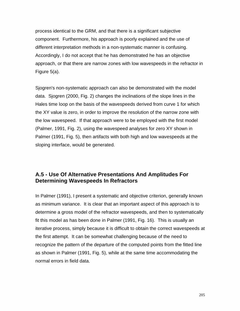
205
process identical to the GRM, and that there is a significant subjective
component. Furthermore, his approach is poorly explained and the use of
different interpretation methods in a non-systematic manner is confusing.
Accordingly, I do not accept that he has demonstrated he has an objective
approach, or that there are narrow zones with low wavespeeds in the refractor in
Figure 5(a).
Sjogren's non-systematic approach can also be demonstrated with the model
data. Sjogren (2000, Fig. 2) changes the inclinations of the slope lines in the
Hales time loop on the basis of the wavespeeds derived from curve 1 for which
the XY value is zero, in order to improve the resolution of the narrow zone with
the low wavespeed. If that approach were to be employed with the first model
(Palmer, 1991, Fig. 2), using the wavespeed analyses for zero XY shown in
Palmer (1991, Fig. 5), then artifacts with both high and low wavespeeds at the
sloping interface, would be generated.
A.5 - Use Of Alternative Presentations And Amplitudes ForDetermining Wavespeeds In Refractors
In Palmer (1991), I present a systematic and objective criterion, generally known
as minimum variance. It is clear that an important aspect of this approach is to
determine a gross model of the refractor wavespeeds, and then to systematically
fit this model as has been done in Palmer (1991, Fig. 16). This is usually an
iterative process, simply because it is difficult to obtain the correct wavespeeds at
the first attempt. It can be somewhat challenging because of the need to
recognize the pattern of the departure of the computed points from the fitted line
as shown in Palmer (1991, Fig. 5), while at the same time accommodating the
normal errors in field data.
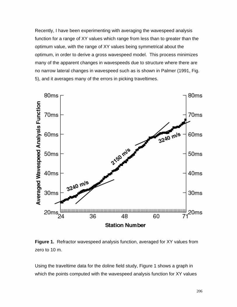
206
Recently, I have been experimenting with averaging the wavespeed analysis
function for a range of XY values which range from less than to greater than the
optimum value, with the range of XY values being symmetrical about the
optimum, in order to derive a gross wavespeed model. This process minimizes
many of the apparent changes in wavespeeds due to structure where there are
no narrow lateral changes in wavespeed such as is shown in Palmer (1991, Fig.
5), and it averages many of the errors in picking traveltimes.
Figure 1. Refractor wavespeed analysis function, averaged for XY values from
zero to 10 m.
Using the traveltime data for the doline field study, Figure 1 shows a graph in
which the points computed with the wavespeed analysis function for XY values
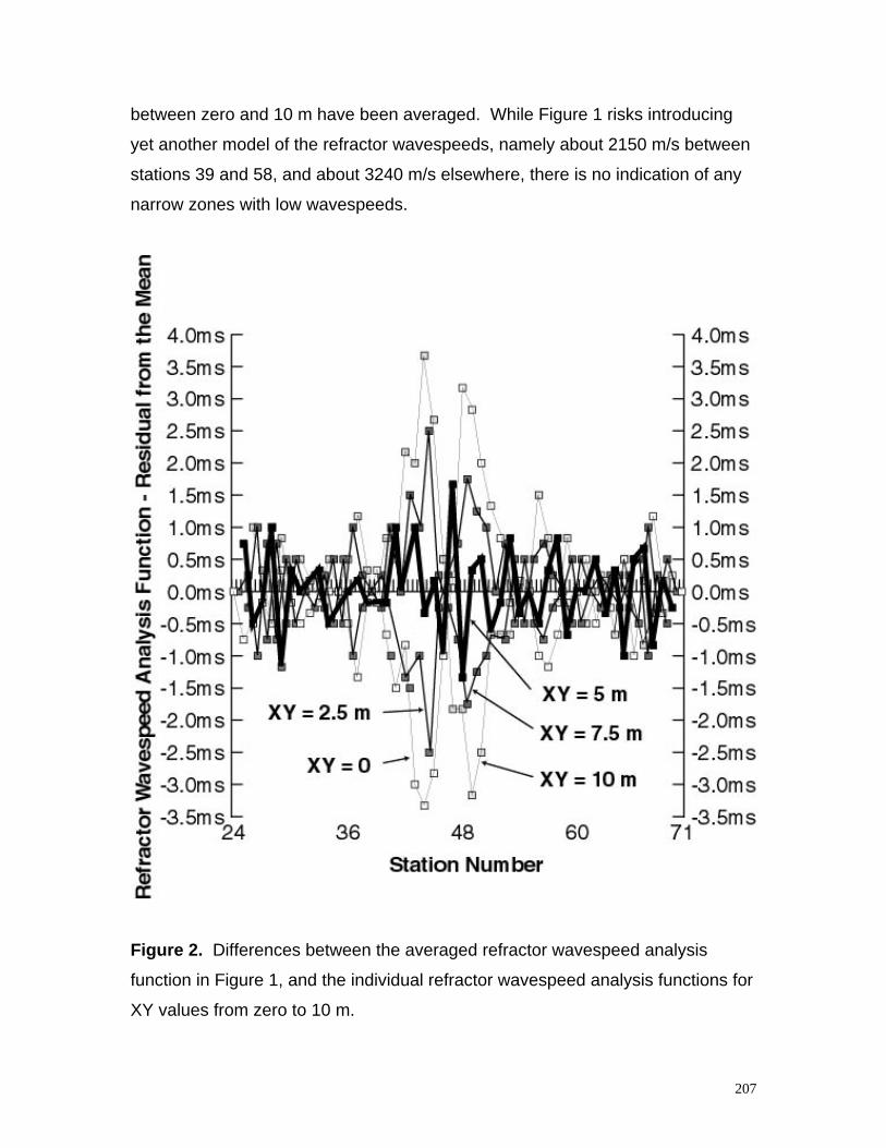
207
between zero and 10 m have been averaged. While Figure 1 risks introducing
yet another model of the refractor wavespeeds, namely about 2150 m/s between
stations 39 and 58, and about 3240 m/s elsewhere, there is no indication of any
narrow zones with low wavespeeds.
Figure 2. Differences between the averaged refractor wavespeed analysis
function in Figure 1, and the individual refractor wavespeed analysis functions for
XY values from zero to 10 m.
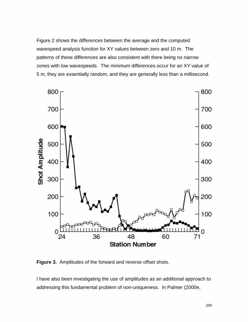
208
Figure 2 shows the differences between the average and the computed
wavespeed analysis function for XY values between zero and 10 m. The
patterns of these differences are also consistent with there being no narrow
zones with low wavespeeds. The minimum differences occur for an XY value of
5 m, they are essentially random, and they are generally less than a millisecond.
Figure 3. Amplitudes of the forward and reverse offset shots.
I have also been investigating the use of amplitudes as an additional approach to
addressing this fundamental problem of non-uniqueness. In Palmer (2000e,
209
2000f), I demonstrate that the amplitude of the refracted head wave, after
correction for geometrical spreading and refractor dip with either convolution or
multiplication, is essentially a function of the head coefficient. I further
demonstrate that the head coefficient is approximately proportional to the ratio of
the specific acoustic impedances (which is the product of the wavespeed and
density) in the overburden to that in the refractor. Therefore, arrivals from zones
in the refractor with low wavespeeds should exhibit high amplitudes, and vice
versa.
The amplitudes for the shot records are shown in Figure 3. For the shot at
station 1, the amplitudes shown a strong decay between stations 24 and 40,
which is interpreted as the geometric effect, together with an interval with
extremely low amplitudes between stations 46 and 59. The amplitudes for the
reverse shot at station 97 show a much less pronounced geometric effect, but
again there is an interval with very low amplitudes between stations 38 and 44.
These very low amplitudes were a major limitation on the measurement of
accurate and consistent traveltimes.
There are very few model studies on the effects of structure on the refraction
amplitudes. Nevertheless, it is unlikely that the very low amplitudes are
compatible with the simple refraction of energy from under the survey profile, but
rather with some form of scattering. They are compatible with energy
propagating around the doline and being scattered back to the surface through
the highly attenuating medium of the rubble in the collapsed doline, as has been
proposed in Palmer (1991).
Figure 4 shows the product of the amplitudes computed with an XY separation of
5 m. The results can be broadly separated into three regions which correspond
approximately with those recognized in Figure 1 with the wavespeed analysis
function. They include high values between stations 24 and 37, very low values
between stations 37 and 59, and higher values between stations 59 and 71. The
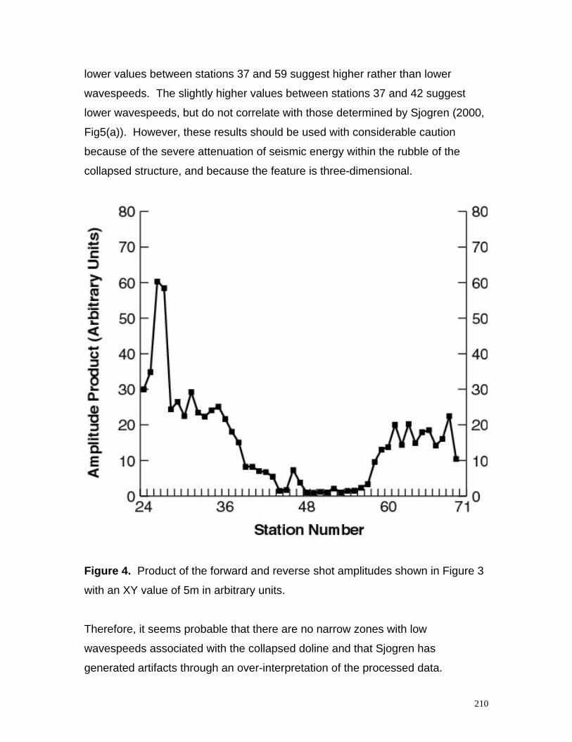
210
lower values between stations 37 and 59 suggest higher rather than lower
wavespeeds. The slightly higher values between stations 37 and 42 suggest
lower wavespeeds, but do not correlate with those determined by Sjogren (2000,
Fig5(a)). However, these results should be used with considerable caution
because of the severe attenuation of seismic energy within the rubble of the
collapsed structure, and because the feature is three-dimensional.
Figure 4. Product of the forward and reverse shot amplitudes shown in Figure 3
with an XY value of 5m in arbitrary units.
Therefore, it seems probable that there are no narrow zones with low
wavespeeds associated with the collapsed doline and that Sjogren has
generated artifacts through an over-interpretation of the processed data.
211
A.6 - A Systematic Approach With The GRM
In summary, Sjogren concludes that “the GRM must be regarded as being of
limited use for detailed and accurate interpretations of refraction seismics for
engineering purposes.” This conclusion is surprising given the very close
similarities between the GRM, Hales’ and the mean-minus-T methods, the latter
two of which he clearly favours. The fact that key features of his figures bear a
remarkable resemblance to parts of the GRM presentations emphasizes the
essential similarities between the two approaches. Instead, he has sought
differences where none really exist, and as a corollary, he has not recognized
similarities where in reality there are many. On the basis of the fundamental
similarities between the GRM and Sjogren's processed data, I conclude that
Sjogren (2000) is more a demonstration of his interpretation style and experience
using a collection of methods rather than a cohesive assessment of the GRM.
However, his approach is neither systematic nor entirely objective, and as a
result it is prone to the generation of artifacts.
It seems that the aim of his paper is to emphasize minor differences, mainly in
the assignment of layers to the traveltime graphs, and then to illogically imply
fundamental shortcomings of the GRM. As such, his paper lacks balance and
objectivity, and it is more in keeping with seeking a conviction in an adversarial
court system than with a scientific journal.
Sjogren (2000) has produced nothing of substance which requires any
fundamental re-assessment of the main features of the GRM in general, or of
Palmer (1991), in particular. He has not satisfactorily addressed the aims of
Palmer (1991), namely an objective method for the recognition and definition of
narrow zones with low wavespeeds. His conclusion that the GRM is unsuitable
for geotechnical applications is not substantiated, and it is based on an
212
incomplete understanding of the GRM and of Palmer (1991), rather than any
genuine shortcomings with the method.
A.7 - The Need To Promote Innovation In Shallow RefractionSeismology
Sjogren’s rejection of the GRM as a useful method for processing and
interpreting shallow seismic refraction data, does little to encourage others to
present new approaches through fear of biased criticism. It is irresponsible and
does not advance the science through balanced and objective debate. In the last
fifty years, innovation in shallow refraction seismology has been rather modest at
best and it has focused predominantly on the various competing methods for
inverting field data. Until there is widespread consensus through a recognition of
fundamental similarities between these inversion methods, there will be little
advancement in other equally important aspects of the science. By comparison,
reflection seismology has achieved major advances through the development of
common midpoint methods, digital signal processing, three-dimensional methods
and sophisticated computer interpretation programs, over the same period of
time. It is now time to move on to the refraction techniques which will be
appropriate to the requirements and the technology of the new millennium.
In Palmer (2000g), I demonstrate the generation of the refraction convolution
section (RCS) through the convolution of forward and reverse traces. The
addition of the traveltimes with convolution is equivalent to that achieved
graphically with Hales’ method and arithmetically with the GRM. The RCS
facilitates full trace processing of seismic refraction data and in turn, the
examination of many important issues such as signal-to-noise ratios, “amplitude
statics”, 3D refraction methods and azimuthal anisotropy, signal processing to
enhance second and later events and stacking data in a manner similar to CMP
reflection methods. A major advantage of the RCS is that it incorporates
213
amplitudes and time structure within a single presentation, facilitating the
resolution of many of the non-uniqueness issues discussed here. It is extremely
rapid and suitable for use with any volume of data, and therefore it can be readily
included in the processing of refraction data with any method.
The RCS is a new approach to obtaining more and better information from
shallow seismic refraction data, and in time it may even supercede the GRM as
well as Hales’ method. However, that possibility can only occur if there is a shift
in culture from one of conflict and an emphasis on minor differences to one of
consensus and an emphasis on fundamental similarities which traditionally, has
characterized the scientific method.
Sjogren’s critique of the GRM does not seek the consensus essential for the
advancement of the science of shallow refraction seismology. Regrettably, it is
neither balanced nor objective, it shows minimal insight into the fundamental
similarities of most methods of refraction inversion, it does not provide an
alternative systematic approach to refraction interpretation, it does not address
the important issues of non-uniqueness, and it does not provide a vision for
future innovation.
A.8 - References
Dobrin, M. B., 1976, Introduction to geophysical prospecting, 3rd edition:
McGraw-Hill Inc.
Oldenburg, D. W., 1984, An introduction to linear inverse theory: Transactions
IEEE Geoscience and Remote Sensing, GE-22(6), 666.
Palmer, D., 1980, The generalized reciprocal method of seismic refraction
interpretation: Society of Exploration Geophysicists.
214
Palmer, D., 1981, An introduction to the generalized reciprocal method of seismic
refraction interpretation: Geophysics 46, 1508-1518
Palmer, D., 1986, Refraction seismics: the lateral resolution of structure and
seismic velocity: Geophysical Press.
Palmer, D., 1991, The resolution of narrow low-velocity zones with the
generalized reciprocal method: Geophysical Prospecting 39, 1031-1060.
Palmer, D, 1992, Is forward modeling as efficacious as minimum variance for
refraction inversion?: Exploration Geophysics, 23, 261-266, 521.
Palmer, D., 1995, Can linear inversion achieve detailed refraction statics?:
Exploration Geophysics, 26, 506-511.
Palmer, D., Goleby, B., and Drummond, B., 2000a, The effects of spatial
sampling on refraction statics: Exploration Geophysics, 31, 270-274.
Palmer, D., 2000a, Model determination for refraction inversion: submitted.
Palmer, D., 2000b, The measurement of weak anisotropy with the generalized
reciprocal method: Geophysics, 65, 1583-1591.
Palmer, D., 2000c, Can amplitudes resolve ambiguities in refraction inversion?:
Exploration Geophysics 31, 304-309.
Palmer, D., 2000d, Starting models for refraction inversion: submitted.
Palmer, D., 2000e, Imaging refractors with the convolution section: Geophysics,
in press.
215
Palmer, D., 2000f, Resolving refractor ambiguities with amplitudes: Geophysics,
in press.
Palmer, D, 2000g, Digital processing of shallow seismic refraction data with the
refraction convolution section, PhD thesis, UNSW, submitted.
Sjogren, B., 2000, A brief study of the generalized reciprocal method and of
some limitations of the method: Geophysical Prospecting 48, 815-834.
Treitel, S., and Lines, L., 1988, Geophysical examples of inversion (with a grain
of salt): The Leading Edge 7, 32-35.
216
Appendix 2
Model Determination For RefractionInversion
A.1 - Summary
In recent years, tomography or model-based inversion, has been used to
construct a model of the subsurface from seismic refraction data, mainly to
determine statics corrections for reflection data. With these methods, the
parameters of a model of the subsurface are refined by comparing the
traveltimes of the model with the field data. When the differences between the
computed and field traveltimes are a minimum, the model and parameters are
taken as an accurate representation of the wavespeeds in the subsurface.
In this study I demonstrate the sensitivity of model-based inversion to the
selection of the inversion model, using eleven geological models. In general, the
residuals between the original and modeled traveltimes are better than 0.4%,
indicating that virtually any model can be fitted to the data with high accuracy.
However, the errors in depth computations are between 5% and 10% for simple
monotonic increases of wavespeed with depth. For other models such as a
reversal in wavespeed, the errors are indeterminate, but much larger. The depth
errors are least when the inversion model and the original geological model are
similar, and greatest when the models are different.
217
I also determine the parameters for the same eleven inversion models with the
generalized reciprocal method (GRM). With the GRM, the parameters of each
model are constrained with the optimum XY value. The errors in depth
computations are generally about one third of those for the equivalent model-
based case. Furthermore, the GRM is able to produce reasonable results with
the wavespeed reversal and transverse isotropy models, unlike the model-based
methods. However, the residuals between the direct traveltimes for the inversion
model and the original geological model are up to a factor of four greater than
with the equivalent model-based case. The residuals are least when the models
are similar, and greatest when the models are different.
The GRM determines model parameters by interpolation with the optimum XY
value. This parameter is determined from the refracted traveltimes from the
underlying layer, and therefore it is a function of all wavespeeds and thicknesses
in the overlying layer(s). By contrast, the model-based methods determine the
model parameters from the direct traveltimes from the upper part of the layer(s),
and then extrapolate those parameters throughout the remainder of the layer(s)
I conclude that suitable starting models for tomographic or model-based
inversion have parameters which are determined with optimum XY values, and
which have minimum residuals between the field and modeled traveltimes of the
direct arrivals.
A.2 - Introduction
In recent years, model-based inversion or tomography, has been used to process
seismic refraction data, often to determine statics corrections for reflection data
(Zhu et al., 1992). With these methods, the parameters of a model of the
subsurface are refined by comparing the traveltimes of the model with the field
data. When the differences between the computed and field traveltimes are a
218
minimum, the model and parameters are taken as an accurate representation of
the wavespeeds in the subsurface.
While the performance of refraction tomography has been continually improved
through more efficient inversion and forward modeling routines, (see Zhang and
Toksoz, 1998 for an overview of these advances), one issue, which has yet to
receive widespread attention, is the choice of the model for the inversion
process. This situation is not surprising, since the role of model-based inversion
is to provide information about the unknown numerical parameters which go into
the model, not to provide the model itself (Menke, 1989, p3).
Perhaps the most common model has been the linear increase of wavespeed
with depth (Zhu et al.,1992; Stefani, 1995; Miller et al., 1998; Lanz et al., 1998),
possibly because of mathematical convenience. However, this model is of
questionable validity as most theoretical (Iida, 1939; Gassman, 1951, 1953;
Brandt, 1955; Paterson, 1956; Berry1959), laboratory (Birch, 1960; Wyllie et al.,
1956, 1958), and field studies (Faust, 1951, 1953; White and Sengbush, 1953;
Acheson, 1963, 1981; Hall, 1970; Hamilton, 1970, 1971; Jankowsky, 1970),
suggest a more gentle increase for clastic sediments, such as a one sixth power
of depth function.
Furthermore, the gradients obtained range from 0.342 and 2.5 m/s per metre
(Stefani, 1995), and 2.68 and 4.67 m/s per metre (Zhu et al., 1992), to as high as
40 m/s per metre (Lanz et al, 1998). These values are generally larger than
those applicable to the compaction of clastic sediments (Dobrin, 1976), but they
are rarely justified on geological or petrophysical grounds.
The combination of the linear increase of wavespeed with depth and the high
gradients probably contributes to instability in the inversion process. The
example of the somewhat paradoxical situation of the poor determination of
wavespeeds in the refractor, despite the fact that over 90% of traveltimes are
219
from that layer (Lanz et al., 1998), is at variance with the experiences of most
seismologists using more traditional methods of refraction processing.
In this study, I demonstrate the effects of the choice of the model on refraction
inversion using both the model-based approach and the generalized reciprocal
method (GRM), (Palmer, 1980, 1986). With the model-based approach, I show
that a range of models can be fitted to noise-free traveltime data with acceptable
accuracy, but that there is a wide range in the depths computed to the main
refractor. However, the accuracy of depth computations improves as the
inversion model approaches the subsurface or geological model. In addition,
only a limited number of models can be examined with model-based methods of
inversion.
With the GRM approach, I show that a wider range of models can be addressed,
with generally greater accuracies in depth computations. However, in contrast
with the methods of model-based inversion, the agreement with the traveltime
data is usually much poorer.
I conclude that the appropriate starting model for tomographic inversion is one for
which the depths are similar to those obtained with the GRM, and for which the
field and model traveltimes agree.
A.3 - Model and Inversion Strategies
The model of the subsurface used in this study is shown in Figure A.1, and
consists of two layers with the upper layer having a parabolic variation in
wavespeed with depth, viz.
V(z) = 1750(1 + 0.001 z)½ (A.1)
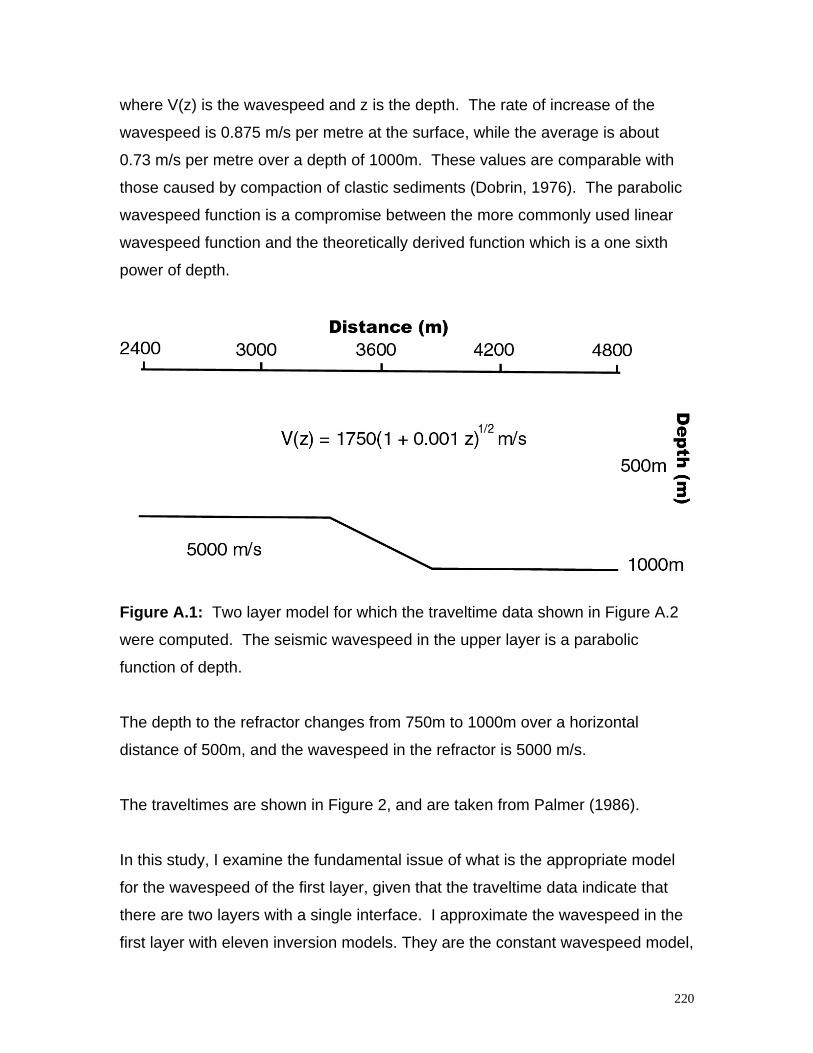
220
where V(z) is the wavespeed and z is the depth. The rate of increase of the
wavespeed is 0.875 m/s per metre at the surface, while the average is about
0.73 m/s per metre over a depth of 1000m. These values are comparable with
those caused by compaction of clastic sediments (Dobrin, 1976). The parabolic
wavespeed function is a compromise between the more commonly used linear
wavespeed function and the theoretically derived function which is a one sixth
power of depth.
Figure A.1: Two layer model for which the traveltime data shown in Figure A.2
were computed. The seismic wavespeed in the upper layer is a parabolic
function of depth.
The depth to the refractor changes from 750m to 1000m over a horizontal
distance of 500m, and the wavespeed in the refractor is 5000 m/s.
The traveltimes are shown in Figure 2, and are taken from Palmer (1986).
In this study, I examine the fundamental issue of what is the appropriate model
for the wavespeed of the first layer, given that the traveltime data indicate that
there are two layers with a single interface. I approximate the wavespeed in the
first layer with eleven inversion models. They are the constant wavespeed model,
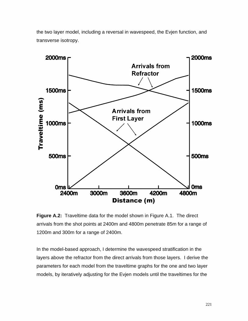
221
the two layer model, including a reversal in wavespeed, the Evjen function, and
transverse isotropy.
Figure A.2: Traveltime data for the model shown in Figure A.1. The direct
arrivals from the shot points at 2400m and 4800m penetrate 85m for a range of
1200m and 300m for a range of 2400m.
In the model-based approach, I determine the wavespeed stratification in the
layers above the refractor from the direct arrivals from those layers. I derive the
parameters for each model from the traveltime graphs for the one and two layer
models, by iteratively adjusting for the Evjen models until the traveltimes for the
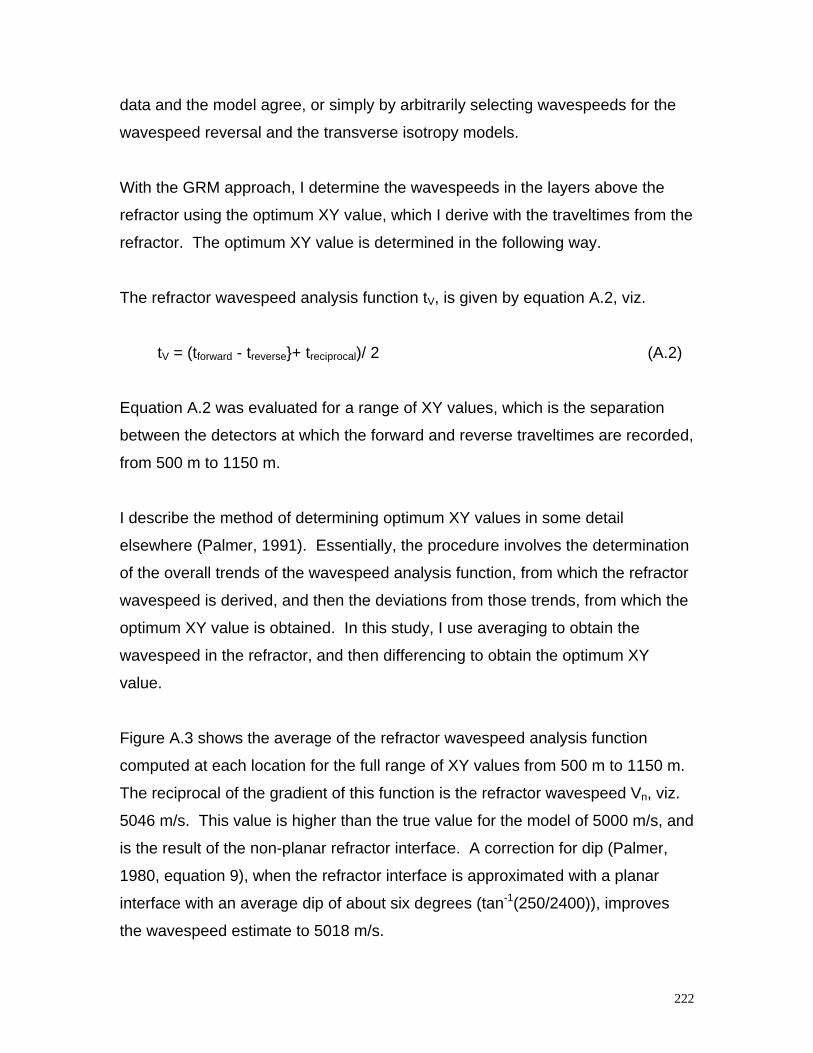
222
data and the model agree, or simply by arbitrarily selecting wavespeeds for the
wavespeed reversal and the transverse isotropy models.
With the GRM approach, I determine the wavespeeds in the layers above the
refractor using the optimum XY value, which I derive with the traveltimes from the
refractor. The optimum XY value is determined in the following way.
The refractor wavespeed analysis function tV, is given by equation A.2, viz.
tV = (tforward - treverse}+ treciprocal)/ 2 (A.2)
Equation A.2 was evaluated for a range of XY values, which is the separation
between the detectors at which the forward and reverse traveltimes are recorded,
from 500 m to 1150 m.
I describe the method of determining optimum XY values in some detail
elsewhere (Palmer, 1991). Essentially, the procedure involves the determination
of the overall trends of the wavespeed analysis function, from which the refractor
wavespeed is derived, and then the deviations from those trends, from which the
optimum XY value is obtained. In this study, I use averaging to obtain the
wavespeed in the refractor, and then differencing to obtain the optimum XY
value.
Figure A.3 shows the average of the refractor wavespeed analysis function
computed at each location for the full range of XY values from 500 m to 1150 m.
The reciprocal of the gradient of this function is the refractor wavespeed Vn, viz.
5046 m/s. This value is higher than the true value for the model of 5000 m/s, and
is the result of the non-planar refractor interface. A correction for dip (Palmer,
1980, equation 9), when the refractor interface is approximated with a planar
interface with an average dip of about six degrees (tan-1(250/2400)), improves
the wavespeed estimate to 5018 m/s.
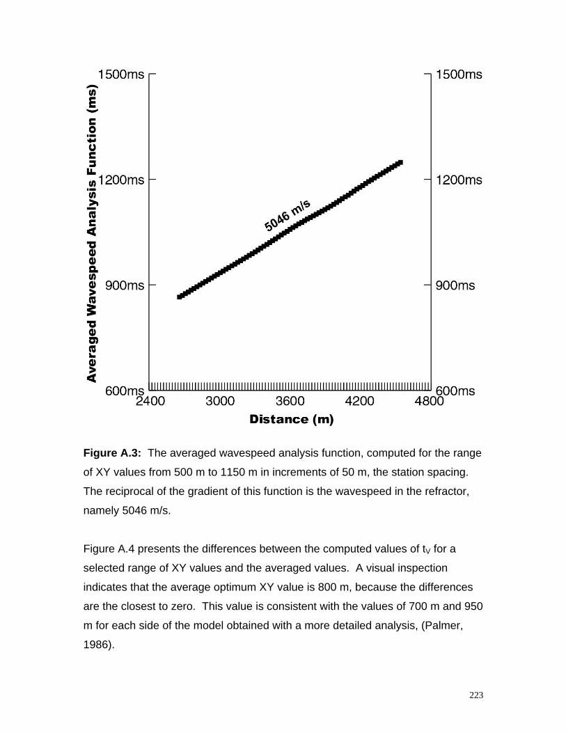
223
Figure A.3: The averaged wavespeed analysis function, computed for the range
of XY values from 500 m to 1150 m in increments of 50 m, the station spacing.
The reciprocal of the gradient of this function is the wavespeed in the refractor,
namely 5046 m/s.
Figure A.4 presents the differences between the computed values of tV for a
selected range of XY values and the averaged values. A visual inspection
indicates that the average optimum XY value is 800 m, because the differences
are the closest to zero. This value is consistent with the values of 700 m and 950
m for each side of the model obtained with a more detailed analysis, (Palmer,
1986).
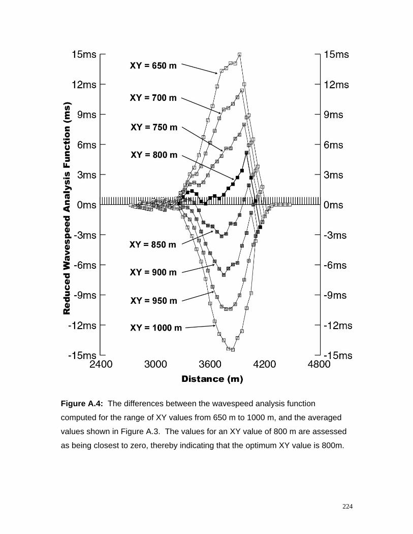
224
Figure A.4: The differences between the wavespeed analysis function
computed for the range of XY values from 650 m to 1000 m, and the averaged
values shown in Figure A.3. The values for an XY value of 800 m are assessed
as being closest to zero, thereby indicating that the optimum XY value is 800m.
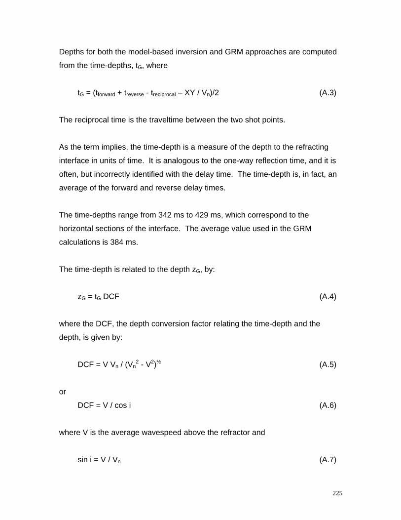
225
Depths for both the model-based inversion and GRM approaches are computed
from the time-depths, tG, where
tG = (tforward + treverse - treciprocal – XY / Vn)/2 (A.3)
The reciprocal time is the traveltime between the two shot points.
As the term implies, the time-depth is a measure of the depth to the refracting
interface in units of time. It is analogous to the one-way reflection time, and it is
often, but incorrectly identified with the delay time. The time-depth is, in fact, an
average of the forward and reverse delay times.
The time-depths range from 342 ms to 429 ms, which correspond to the
horizontal sections of the interface. The average value used in the GRM
calculations is 384 ms.
The time-depth is related to the depth zG, by:
zG = tG DCF (A.4)
where the DCF, the depth conversion factor relating the time-depth and the
depth, is given by:
DCF = V Vn / (Vn2 - V2)½ (A.5)
or
DCF = V / cos i (A.6)
where V is the average wavespeed above the refractor and
sin i = V / Vn (A.7)
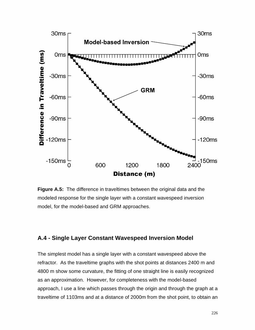
226
Figure A.5: The difference in traveltimes between the original data and the
modeled response for the single layer with a constant wavespeed inversion
model, for the model-based and GRM approaches.
A.4 - Single Layer Constant Wavespeed Inversion Model
The simplest model has a single layer with a constant wavespeed above the
refractor. As the traveltime graphs with the shot points at distances 2400 m and
4800 m show some curvature, the fitting of one straight line is easily recognized
as an approximation. However, for completeness with the model-based
approach, I use a line which passes through the origin and through the graph at a
traveltime of 1103ms and at a distance of 2000m from the shot point, to obtain an
227
average wavespeed of 1813 m/s. The differences in the traveltimes for the data
and the constant wavespeed model range from -16 ms to 19 ms, and are shown
in Figure A.5. These residuals are comparable to those obtained by Stefani
(1995) with the Tibalier Trench data which is at approximately the same depth.
Accordingly, I view the fit between the computed and original data as acceptable.
Figure A.6: Unmigrated depth sections for the single layer with a constant
wavespeed inversion model, for the model-based and GRM approaches.
The depths computed with this wavespeed are shown in Figure A.6, and they
have been plotted vertically, rather than orthogonally to the refractor interface.
228
An additional step, equivalent to the migration operation of reflection data, is
required to accurately image the refractor interface (Palmer, 1986, p.196-198).
The depths computed over the horizontal sections of the refractor are 659.4m
(for an error of -12.1%), and 833.4m (for an error of -16.7%), and they are listed
in Table A.1.
The GRM approach uses the average velocity formula (Palmer, 1980, p.42, eqn.
27; 1986, p.147, eqn. 10.4), for the single layer, constant wavespeed model,
viz.
V = [(XY Vn2) / (XY + 2 tG Vn)]½ (A.8)
The resultant average wavespeed is 2107 m/s, which in turn produces depths
over the horizontal sections of 770.2 m (for an error of 2.7%) and 973.6 m (for an
error of -2.6%). The differences in the traveltimes for the data and the constant
wavespeed model range from zero to -140 ms, and are shown in Figure A.5.
This inversion model emphasizes the appropriateness of the selection of the
starting model with model-based inversion. The constant wavespeed model is
applicable to a wide range a subsurface targets especially those in the near
surface, and it has proven to be efficacious since the earliest days of refraction
seismology. Furthermore, it is often used for field data, where the curvature of
the traveltime graph is not obvious (Palmer, 1983; Zhu et al., 1992). This
situation is not uncommon because the amplitudes at the larger offsets are
usually much weaker than those on the near offsets, thereby resulting in the
arrival times being measured later than is the case with noise-free data.
Even though the differences in the traveltimes between field and the modeled
data are an order of magnitude smaller with the model-based inversion approach
than with the GRM, there is not a commensurate improvement in the depth
computations.
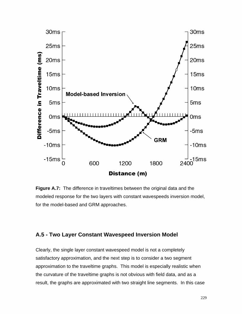
229
Figure A.7: The difference in traveltimes between the original data and the
modeled response for the two layers with constant wavespeeds inversion model,
for the model-based and GRM approaches.
A.5 - Two Layer Constant Wavespeed Inversion Model
Clearly, the single layer constant wavespeed model is not a completely
satisfactory approximation, and the next step is to consider a two segment
approximation to the traveltime graphs. This model is especially realistic when
the curvature of the traveltime graphs is not obvious with field data, and as a
result, the graphs are approximated with two straight line segments. In this case
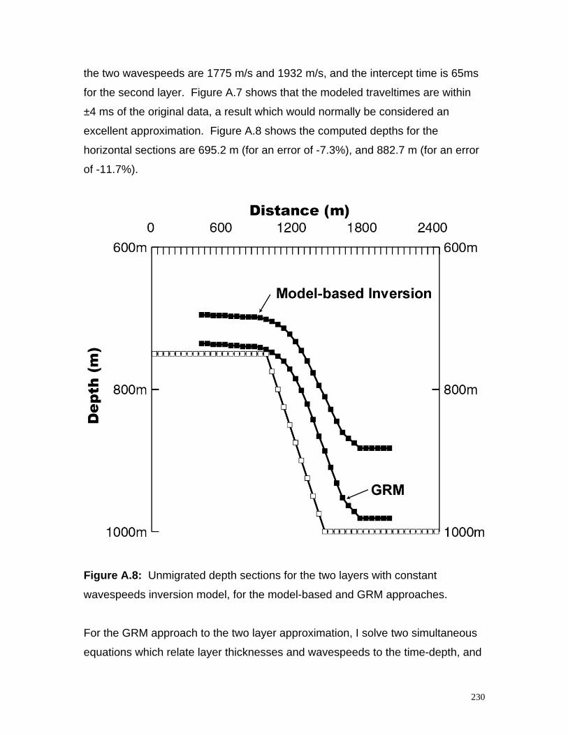
230
the two wavespeeds are 1775 m/s and 1932 m/s, and the intercept time is 65ms
for the second layer. Figure A.7 shows that the modeled traveltimes are within
±4 ms of the original data, a result which would normally be considered an
excellent approximation. Figure A.8 shows the computed depths for the
horizontal sections are 695.2 m (for an error of -7.3%), and 882.7 m (for an error
of -11.7%).
Figure A.8: Unmigrated depth sections for the two layers with constant
wavespeeds inversion model, for the model-based and GRM approaches.
For the GRM approach to the two layer approximation, I solve two simultaneous
equations which relate layer thicknesses and wavespeeds to the time-depth, and
231
to the optimum XY value, (Palmer, 1980, p.47: 1986, p.136-137). The results are
the layer thicknesses z1 and z2, after values for the wavespeeds have been set.
The equations are:
tG = z1 cos i1n / V1 + z2 cos i2n / V2 (A.9)
XY = 2 z1 tan i1n + 2 z2 tan i2n (A.10)
where
ijn = sin-1 (Vj / Vn) (A.11)
The values used for the wavespeeds are 1800 m/s for V1, which is suggested by
the traveltime graphs, and 2400 m/s for V2. The computed depths are 735.7 m
(for an error of -1.9%), and 981.2 m (for an error of -1.9%).
The traveltime differences are shown in Figure A.7 and range from -10 ms to +25
ms. As with the single layer inversion model, these differences are much larger
than those for the model-based inversion approach, but the depth computations
are still more accurate.
A.6 - Two Layer Wavespeed Reversal Inversion Model
Suppose that there were sufficient reasons for considering the existence of a
surface layer with a wavespeed of 3600 m/s. In this case, the traveltime graphs
with the shot points at 2400m and 4800m, would be ignored because of
additional, more compelling reasons, such as the existence of a local surface
lens of limestone or permafrost with a high wavespeed, or even extrapolation
from an adjacent area. The model-based inversion approach can only assume
232
that this wavespeed occurs throughout the upper layer, resulting in computed
depths of 1758.6 m (for an error of 137%) and 2222.8 m (for an error of 123%).
The GRM approach to the wavespeed reversal model is similar to the two layer
constant wavespeed model described previously. In that case, the selection of
the second layer wavespeed of 2400 m/s might have appeared to be rather
arbitrary. In fact, almost any wavespeed will suffice, provided it is above a
certain minimum, because the thickness of the corresponding layer is
automatically adjusted to produce an effective average wavespeed similar to that
obtained with equation A.4. Furthermore, it will be noted that there is no
requirement for the wavespeeds to increase monotonically with depth with this
approach, and therefore it can be applied equally validly to the wavespeed
reversal model. Using wavespeeds of 3600 m/s and 1800 m/s, solution of
equations A.9 to A.11 produces depths of 731.81 m (for an error of -2.4%), and
904.7m (for an error of -9.5%).
The wavespeed reversal model is generally acknowledged as one of the most
difficult if not impossible to address satisfactorily with refraction tomography
(Lanz et al., 1998). In the absence of other geological or geophysical data, the
GRM approach provides a measure of constraint for a normally intractable
problem.
A.7 - The Evjen Inversion Model
If in fact, it was recognised that the traveltime data represented a variable
wavespeed medium, then the wavespeed function in the overburden can be
approximated with the Evjen function, viz.
V(z) = V0 (1 + q z)1/m (A.12)
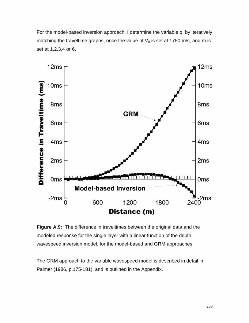
233
For the model-based inversion approach, I determine the variable q, by iteratively
matching the traveltime graphs, once the value of V0 is set at 1750 m/s, and m is
set at 1,2,3,4 or 6.
Figure A.9: The difference in traveltimes between the original data and the
modeled response for the single layer with a linear function of the depth
wavespeed inversion model, for the model-based and GRM approaches.
The GRM approach to the variable wavespeed model is described in detail in
Palmer (1986, p.175-181), and is outlined in the Appendix.
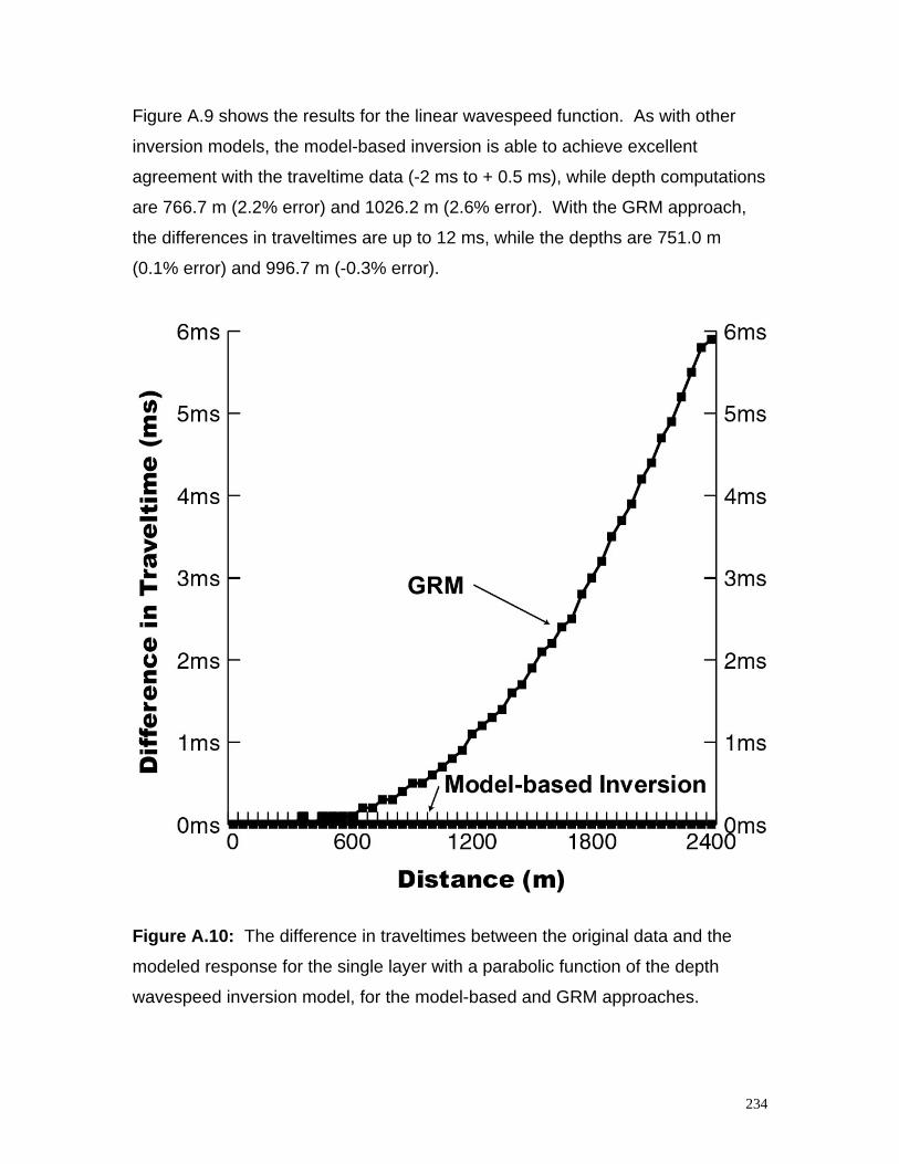
234
Figure A.9 shows the results for the linear wavespeed function. As with other
inversion models, the model-based inversion is able to achieve excellent
agreement with the traveltime data (-2 ms to + 0.5 ms), while depth computations
are 766.7 m (2.2% error) and 1026.2 m (2.6% error). With the GRM approach,
the differences in traveltimes are up to 12 ms, while the depths are 751.0 m
(0.1% error) and 996.7 m (-0.3% error).
Figure A.10: The difference in traveltimes between the original data and the
modeled response for the single layer with a parabolic function of the depth
wavespeed inversion model, for the model-based and GRM approaches.
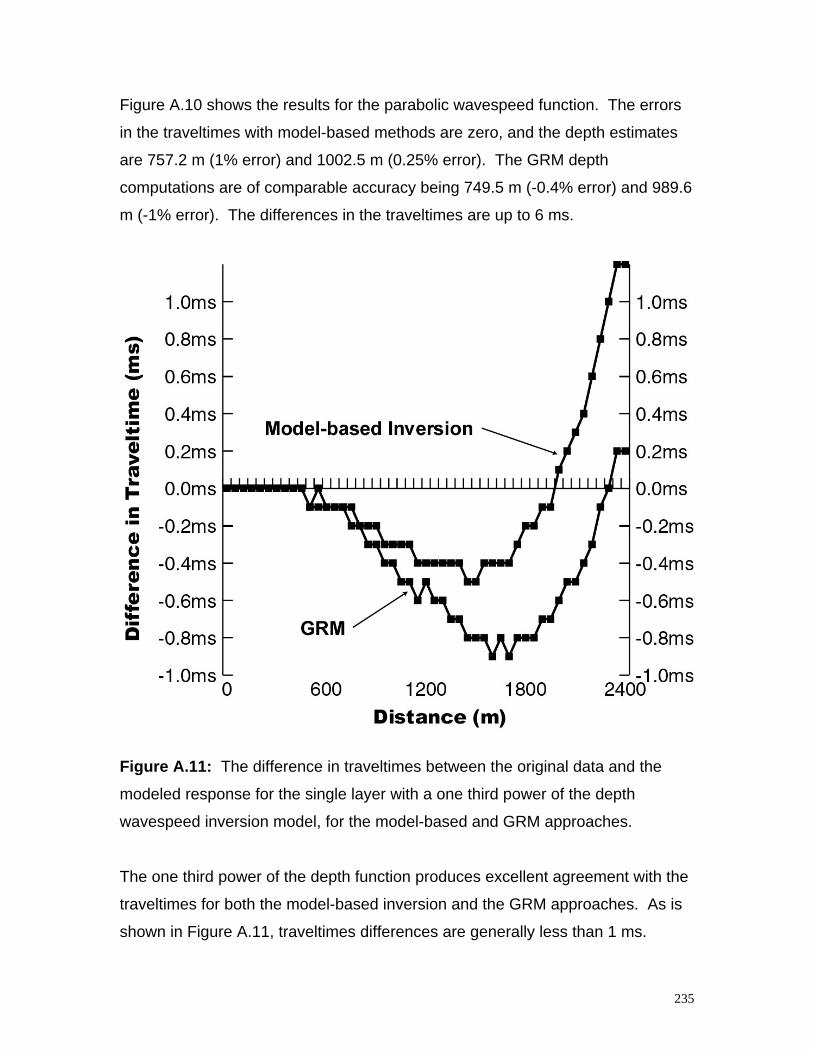
235
Figure A.10 shows the results for the parabolic wavespeed function. The errors
in the traveltimes with model-based methods are zero, and the depth estimates
are 757.2 m (1% error) and 1002.5 m (0.25% error). The GRM depth
computations are of comparable accuracy being 749.5 m (-0.4% error) and 989.6
m (-1% error). The differences in the traveltimes are up to 6 ms.
Figure A.11: The difference in traveltimes between the original data and the
modeled response for the single layer with a one third power of the depth
wavespeed inversion model, for the model-based and GRM approaches.
The one third power of the depth function produces excellent agreement with the
traveltimes for both the model-based inversion and the GRM approaches. As is
shown in Figure A.11, traveltimes differences are generally less than 1 ms.
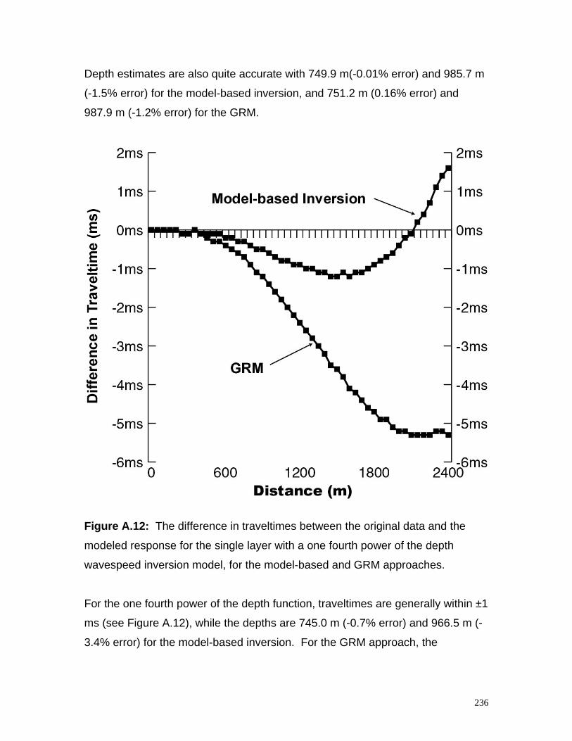
236
Depth estimates are also quite accurate with 749.9 m(-0.01% error) and 985.7 m
(-1.5% error) for the model-based inversion, and 751.2 m (0.16% error) and
987.9 m (-1.2% error) for the GRM.
Figure A.12: The difference in traveltimes between the original data and the
modeled response for the single layer with a one fourth power of the depth
wavespeed inversion model, for the model-based and GRM approaches.
For the one fourth power of the depth function, traveltimes are generally within ±1
ms (see Figure A.12), while the depths are 745.0 m (-0.7% error) and 966.5 m (-
3.4% error) for the model-based inversion. For the GRM approach, the
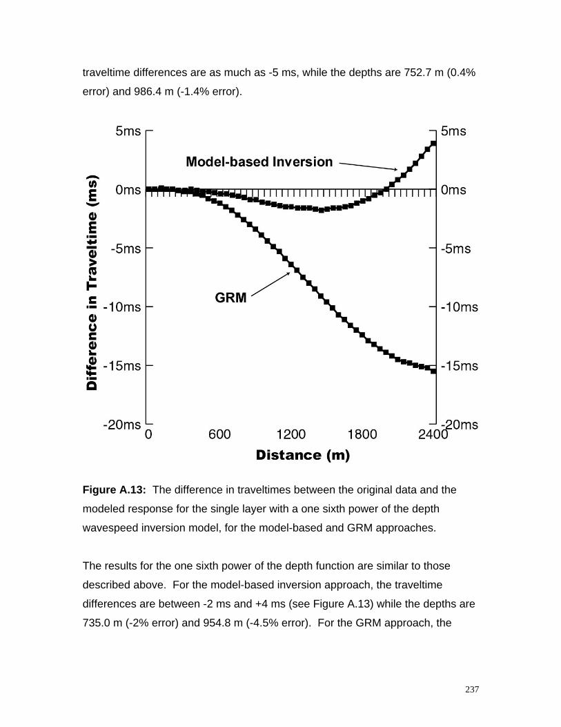
237
traveltime differences are as much as -5 ms, while the depths are 752.7 m (0.4%
error) and 986.4 m (-1.4% error).
Figure A.13: The difference in traveltimes between the original data and the
modeled response for the single layer with a one sixth power of the depth
wavespeed inversion model, for the model-based and GRM approaches.
The results for the one sixth power of the depth function are similar to those
described above. For the model-based inversion approach, the traveltime
differences are between -2 ms and +4 ms (see Figure A.13) while the depths are
735.0 m (-2% error) and 954.8 m (-4.5% error). For the GRM approach, the
238
traveltime differences are up to -15 ms, while depths are 755.2 m (0.7% error)
and 984.4 m (-1.6% error).
A.8 - Transverse Isotropy Inversion Model
Finally, there is the case of seismic anisotropy, in which the horizontal
wavespeed is different from the vertical value. This is one area where the
geophysical idealization of the earth can differ substantially from the
petrophysical reality. While there is overwhelming evidence that wavespeeds are
more likely to be anisotropic than isotropic, because of intrinsic anisotropy, cyclic
layering, etc, it is rare for the basic model for most refraction inversion routines to
include this property. No doubt the complexities of the mathematical treatment,
together with the lack of accepted methods for determining anisotropy
parameters from surface measurements, contribute to this situation.
In most cases, the horizontal wavespeed is greater than the vertical value. This
is usually the case with undisturbed sedimentary rocks, because of the effects of
compaction and cyclic layering. However, the reverse condition may apply, such
as with steeply dipping sedimentary or metamorphic rocks, or with non-
hydrostatic stress. Accordingly, simply assuming an anisotropy factor with the
vertical wavespeed being less than the horizontal can sometimes be
inappropriate.
Unless there is additional information, such as bore hole control, seismic
anisotropy is not easily recognised or accommodated with the standard refraction
methods, and any depth and wavespeed computations can have indeterminate
errors. However, for completeness of the comparison, I use the commonly
assumed anisotropy factor for P waves in sedimentary rocks of 1.10, together
with the horizontal wavespeeds of 1800 m/s, 2100 m/s and 2300 m/s, for the
239
model-based inversion approach. The vertical wavespeeds used for depth
conversion are then 1636 m/s, 1909 m/s and 2091 m/s.
The GRM approach to anisotropic overburdens is described in detail in Palmer
(Palmer, 1986). With this approach, I seek to determine the anisotropy factor,
which is the horizontal wavespeed divided by the vertical wavespeed, for which
the wavespeed given by the Crampin equation, viz.
V2(φ) = A + B cos 2φ + C cos 4φ (A.9)
(where φ is the angle from the vertical), is equal to the average wavespeed
modified for anisotropy, viz.
V = [(XY Vn2) / (XY + 2 c tG Vn)]½ (A.10)
where
c = (A - B + C - 8 C cos4 φ) / (A + B + C - 8 C sin4 φ) (A.11)
The value of φ used in equations A.13 and A.15, is that for the critical angle for
an horizontal refractor. I examine three models of anisotropy.
The first model uses a horizontal wavespeed of 1800 m/s, which can be
recovered from the traveltime graphs. For the model-based inversion approach
using an anisotropy factor of 1.1, the computed depths are 664.3 m (-11.4%
error) and 839.7 m (-16% error).
The GRM approach produces an anisotropy factor of 0.855, and depths of 789.7
(5.3% error) and 998.1 m (-0.2% error). The computed value of the anisotropy
factor is unusual in that it is less than unity. Nevertheless, the computed depths
are reasonably close to the true values.
240
The second model uses a horizontal wavespeed of 2100 m/s, which is
approximately the average wavespeed in the first layer. For the model-based
inversion approach using an anisotropy factor of 1.1, the computed depths are
700.0 m (-6.7% error) and 885.1 m (-11.5% error).
The GRM approach produces an anisotropy factor of 1.025, and depths of 763.0
m (1.7% error) and 965.5 m (-3.5% error). In this case, the anisotropy factor is
close to unity, which is compatible with the selection of a horizontal wavespeed
similar to the average computed with equation A.4. Therefore, the GRM can
produce an isotropic result if indeed that is appropriate.
The third model uses a horizontal wavespeed of 2400 m/s. For the model-based
inversion approach, the computed depths are 780.4 m (4.1% error) and 986.4 m
(-1.4% error). This is the best result for this approach and it is the result of a
fortuitous combination of the horizontal wavespeed and the assumed anisotropy
factor producing a vertical wavespeed which is comparable with the average
computed with equation A.4.
The GRM approach produces an anisotropy factor of 1.21, and depths of 706.9
m (-5.8% error) and 893.6 m (-10.6% error).
Seismic anisotropy, like wavespeed reversals, emphasizes the fact the model-
based inversion is only efficacious when the traveltime data are an accurate and
complete reflection of the subsurface wavespeed stratification, and therefore
when an inversion model can be determined.
241
A.9 - Errors Related to the Optimum XY Value
In general, the errors in the depth computations related to the choice of the
choice of the inversion model, are between 2% to 3% with the GRM approach.
For this study, a single or average optimum XY value is used. I demonstrate
further improvements in accuracy when the optimum XY values, which are
applicable to each side of the sloping segment of the refractor, are used (Palmer,
1986, 1992).
The errors in the depth computations which are related to the errors in the
measurement of the XY value, can be estimated in the following way.
The errors in the optimum XY value are one half of the detector spacing, ie ± 25
m. Therefore the possible range of optimum XY values is 800 m ± 25 m, ie 775
m to 825 m. (An inspection of Figure A.4 suggests that the latter value of 825 m
is probably the best estimate of a single average value. It is also the mean of the
values applicable to either side of the sloping interface (Palmer, 1986).)
The single layer constant wavespeed will be used for convenience. The average
wavespeed computed with equation 4 using optimum XY values of 775 m and
825 m, are 2079 m/s and 2133 m/s. They differ from the value of 2107 m/s used
in the single layer inversion model above, by an average of ± 27 m/s, or about
1.3%. The resulting error in depth calculations is approximately ± 11.4 m or
1.3%.
Alternatively, it can be demonstrated by differentiation of equation A.4 that:
∆V / V ≈ ½ ∆XY / XY (A.16)
Therefore, an error of 3% (25/800) in the optimum XY value, results in an error of
1.5% in the average wavespeed.
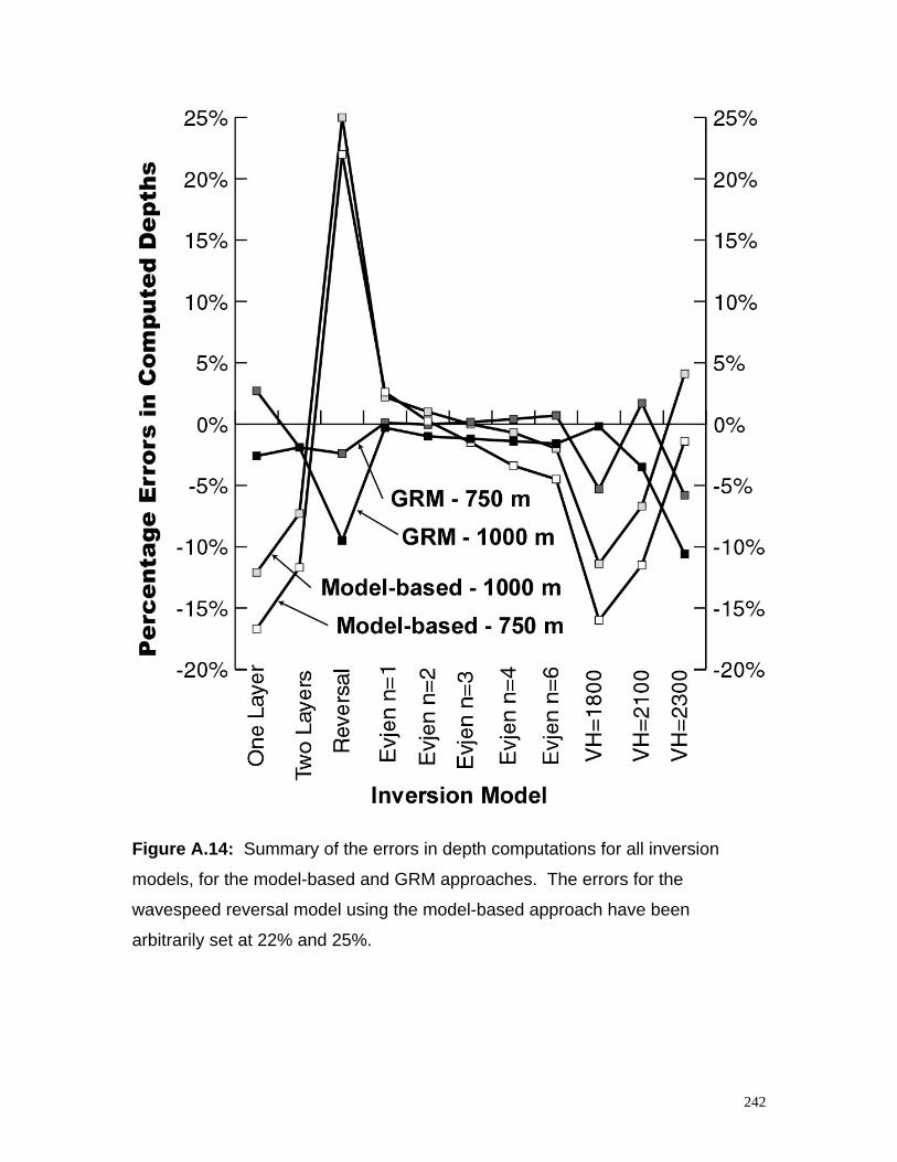
242
Figure A.14: Summary of the errors in depth computations for all inversion
models, for the model-based and GRM approaches. The errors for the
wavespeed reversal model using the model-based approach have been
arbitrarily set at 22% and 25%.
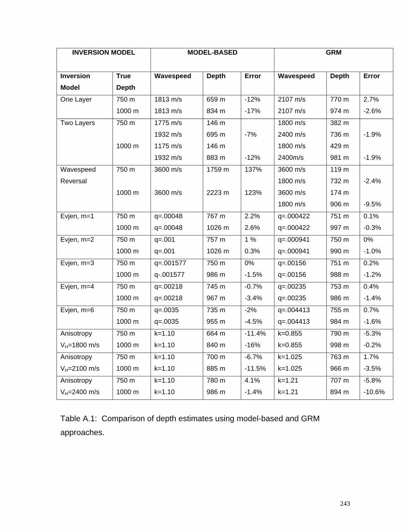
243
INVERSION MODEL MODEL-BASED GRM
InversionModel
TrueDepth
Wavespeed Depth Error Wavespeed Depth Error
One Layer 750 m
1000 m
1813 m/s
1813 m/s
659 m
834 m
-12%
-17%
2107 m/s
2107 m/s
770 m
974 m
2.7%
-2.6%
Two Layers 750 m
1000 m
1775 m/s
1932 m/s
1175 m/s
1932 m/s
146 m
695 m
146 m
883 m
-7%
-12%
1800 m/s
2400 m/s
1800 m/s
2400m/s
382 m
736 m
429 m
981 m
-1.9%
-1.9%
Wavespeed
Reversal
750 m
1000 m
3600 m/s
3600 m/s
1759 m
2223 m
137%
123%
3600 m/s
1800 m/s
3600 m/s
1800 m/s
119 m
732 m
174 m
906 m
-2.4%
-9.5%
Evjen, m=1 750 m
1000 m
q=.00048
q=.00048
767 m
1026 m
2.2%
2.6%
q=.000422
q=.000422
751 m
997 m
0.1%
-0.3%
Evjen, m=2 750 m
1000 m
q=.001
q=.001
757 m
1026 m
1 %
0.3%
q=.000941
q=.000941
750 m
990 m
0%
-1.0%
Evjen, m=3 750 m
1000 m
q=.001577
q-.001577
750 m
986 m
0%
-1.5%
q=.00156
q=.00156
751 m
988 m
0.2%
-1.2%
Evjen, m=4 750 m
1000 m
q=.00218
q=.00218
745 m
967 m
-0.7%
-3.4%
q=.00235
q=.00235
753 m
986 m
0.4%
-1.4%
Evjen, m=6 750 m
1000 m
q=.0035
q=.0035
735 m
955 m
-2%
-4.5%
q=.004413
q=.004413
755 m
984 m
0.7%
-1.6%
Anisotropy
VH=1800 m/s
750 m
1000 m
k=1.10
k=1.10
664 m
840 m
-11.4%
-16%
k=0.855
k=0.855
790 m
998 m
-5.3%
-0.2%
Anisotropy
VH=2100 m/s
750 m
1000 m
k=1.10
k=1.10
700 m
885 m
-6.7%
-11.5%
k=1.025
k=1.025
763 m
966 m
1.7%
-3.5%
Anisotropy
VH=2400 m/s
750 m
1000 m
k=1.10
k=1.10
780 m
986 m
4.1%
-1.4%
k=1.21
k=1.21
707 m
894 m
-5.8%
-10.6%
Table A.1: Comparison of depth estimates using model-based and GRM
approaches.
244
A.10 - Discussion and Conclusions
This study demonstrates that virtually any inversion model can be fitted to
traveltime data to a high accuracy. With the noise-free data used in this study,
the accuracy is generally better than ±5 ms for traveltimes of up to 1300 ms or
0.4%. The errors are about four times larger for the single layer constant
wavespeed inversion model, but they are still acceptable.
However, the superior agreement with the traveltime data is not associated with
more accurate depth estimates. The average errors in depth computations are
about 5% to 10% and they are approximately three times larger than those
obtained through a GRM analysis. Figure A.14 summarizes the results.
In those cases where the inversion models are similar to the test model as with
the Evjen functions, the accuracy of the depth computations is quite high. The
accuracy is highest with the Evjen function with exponents of 2 and 3, which are
close to the test model, and it is least for exponents of 1 and 6, which represent
less similar models.
The lower accuracy of depths computed with the one and two layer
approximations, which are valid and widely applicable inversion models,
indicates the significance of the inversion model rather than the superiority of
variable wavespeed models, such as the linear function. As a corollary, it
indicates that the use of linear functions where constant wavespeed models are
applicable will also result in comparable significant errors in depth computations.
The cases of a reversal in the wavespeed and transverse isotropy illustrate a
fundamental shortcoming of model-based inversion. With a wavespeed reversal,
no traveltimes are recorded from the layer, and therefore it is simply not possible
to achieve agreement between the observed data and the computed traveltimes.
With seismic anisotropy, the traveltimes are obtained in the wrong direction. The
245
field data are a measure of the horizontal wavespeed, while the vertical or near-
vertical wavespeed is required for depth conversion. These models demonstrate
that layers or wavespeeds not represented in the traveltime data can only be
modeled after an empirical assignment of parameters, or only if other data are
available, such as borehole control.
By contrast, the differences between the original traveltime data and the
computed traveltimes for models whose parameters are determined with the
GRM, are much larger. In several cases, these differences can be many tens of
milliseconds or up to 11%. However, the computed depths are generally more
accurate than those computed with the model-based approach. Furthermore, the
GRM is able to address the valid and important inversion models of wavespeed
reversal and transverse isotropy, unlike the model-based methods.
The consistent depth computations with the GRM are related to the constraint of
the wavespeed models with the optimum XY value. This parameter is a function
of both the thicknesses and wavespeeds of all layers above the refractor.
Therefore, the accuracy of the GRM approach is due to the inherent accuracy of
interpolation.
By contrast, the maximum depth of penetration of the direct arrivals used in the
model-based approach is less than 300 m (Palmer, 1986, equation 13.18). As a
result, wavespeeds throughout the first layer are determined by extrapolation
from the upper part of that layer. The various inversion models represent
different extrapolation functions and the errors are due to the inherent instability
of extrapolation. This instability is aggravated where there are undetected layers.
Furthermore, the application of linear wavespeed functions to constant
wavespeed layering can result in large gradients (Lanz et al., 1998), which in turn
can result in the ubiquitous ray path diagrams demonstrating almost complete
coverage of the subsurface. These diagrams are misleading when the inversion
246
model does not accurately represent the subsurface, because the shortcomings
of extrapolation are not overcome.
In general, the direct traveltimes through a layer are unable to provide a reliable
wavespeed model of that layer, except in the trivial cases of isotropic constant
wavespeeds. This casts doubts on the benefits of very high precision of the
traveltimes. Although the data used in this study are noise-free and accurate to
0.1 ms, there is not a corresponding increased accuracy in the depth
computations with the model-based approach. Accordingly, it is questionable
whether it is necessary to measure traveltimes to an accuracy of 0.1 ms (Lanz et
al., 1998), especially when the acceptable residuals appear to be between 2 ms
and 5 ms for most near surface targets.
A more reliable measure of the accuracy of depth computations is the optimum
XY value, because it constrains the parameters for each inversion model. This in
turn, is a function of the detector interval. Therefore, trace spacing is at least as
important as the accuracy of the traveltime data in assessing of the accuracy of
refraction inversion.
While it is clear that the quality of the field data will have some effect on the
measurement of the optimum XY value, it is not as critical as with the model-
based methods. This single parameter is obtained through the recognition of a
distinctive pattern of minimum residuals between the computed and averaged
wavespeed analysis function, as shown in Figure A.4. This pattern is less
sensitive to errors in the individual traveltimes.
The major conclusion to be drawn from this study is that the choice of the
inversion model is an important, if not the most important factor in the
performance of model-based inversion. However, the wavespeed model for
each layer cannot be determined uniquely from the traveltime data from that
layer, because the data generally do not provide a complete, an accurate nor a
247
representative sample of that layer. By contrast, the optimum XY value does
provide a complete sample, because it is determined from the traveltimes for the
underlying refractor, and it is able constrain an almost complete range of
inversion models. Therefore, the appropriate model for model-based inversion
has parameters determined with a GRM analysis, together with minimum
residuals between observed and modeled traveltimes.
The results of this study suggests a two stage inversion strategy. Firstly, the
GRM is employed where the refractor is sufficiently irregular, in order to
determine an appropriate model for inversion. Experience indicates that this
situation occurs in about 30% of the data. Secondly, model-based inversion
methods such as tomography are then employed to process the full set of data,
using the wavespeed model determined with the GRM analysis.
Alternatively, if depth estimates obtained with the GRM using the single layer
constant wavespeed model are similar to those obtained with model-based
inversion, then the inversion model can be taken as appropriate.
A.11 - References
Acheson, C. H., 1963, Time-depth and velocity-depth relations in Western
Canada: Geophysics, 28, 894-909.
Acheson, C. H., 1981, Time-depth and velocity-depth relations in sedimentary
basins - a study based on current investigations in the Arctic Islands and an
interpretation of experience elsewhere: Geophysics, 46, 707-716.
Berry, J. E., 1959, Acoustic velocity in porous media: Petroleum Trans. AIME,
216, 262-270.
248
Birch, F., 1960, The velocity of compressional waves in rocks at 10 kilobars: J.
Geophys. Res., 65, 1083-1102.
Brandt, H., 1955, A study of the speed of sound in porous granular media: J.
Appl. Mech., 22, 479-486
Dobrin, M. B., 1976, Introduction to geophysical prospecting, 3rd edition:
McGraw-Hill Inc.
Faust, L. Y., 1951, Seismic velocity as a function of depth and geologic time:
Geophysics, 16, 192-206.
Faust, L. Y., 1953, A velocity function including lithologic variation: Geophysics,
18, 271-288.
Gassman, F., 1951, Elastic waves through a packing of spheres: Geophysics,
16, 673-685.
Gassman, F., 1953, Note on Elastic waves through a packing of spheres:
Geophysics, 16, 269.
Hall, J., 1970, The correlation of seismic velocities with formations in the
southwest of Scotland: Geophys. Prosp., 18, 134-156.
Hamilton, E. L., 1970, Sound velocity and related properties of marine sediments,
North Pacific: J. Geophys. Res., 75, 4423-4446.
Hamilton, E. L., 1971, Elastic properties of marine sediments: J. Geophys. Res.,
76, 579-604.
249
Iida, K., 1939, Velocity of elastic waves in granular substances: Tokyo Univ.
Earthquake Res. Inst. Bull., 17, 783-897.
Jankowsky, W., 1970, Empirical investigation of some factors affecting elastic
velocities in carbonate rocks: Geophys. Prosp., 18 103-118.
Lanz, E., Maurer, H., and Green, A. G., 1998, Refraction tomography over a
buried waste disposal site: Geophysics, 63, 1414-1433.
Menke, W., 1989, Geophysical data analysis: discrete inverse theory: Academic
Press, Inc.
Miller, K. C., Harder, S. H., and Adams, D. C., and O'Donnell, T., 1998,
Integrating high-resolution refraction data into near-surface seismic reflection
data processing and interpretation: Geophysics, 63, 1339-1347.
Palmer, D., 1980, The generalized reciprocal method of seismic refraction
interpretation: Society of Exploration Geophysicists.
Palmer, D., 1983, Comment on "Curved raypath interpretation of seismic
refraction data" by S.A. Greenhalgh and D.W. King: Geophys. Prosp., 31, 542-
543.
Palmer, D., 1986, Refraction seismics - the lateral resolution of structure and
seismic velocity: Geophysical Press.
Palmer, D., 1991, The resolution of narrow low-velocity zones with the
generalized reciprocal method: Geophys. Prosp., 39, 1031-1060.
Palmer, D., 1992, Is forward modelling as efficacious as minimum variance for
refraction inversion?: Explor. Geophys., 23, 261-266, 521.
250
Paterson, N. R., 1956, Seismic wave propagation in porous granular media:
Geophysics, 21, 691-714.
Stefani, J. P., 1995, Turning-ray tomography: Geophysics, 60, 1917-1929.
White, J. E., and Sengbush, R. L.,, 1953, Velocity measurements in near surface
formations: Geophysics, 18, 54-69.
Wyllie, W. R., Gregory, A. R.,and Gardner, L. W., 1956, Elastic wave velocities in
heterogeneous and porous media: Geophysics, 21, 41-70.
Wyllie, W. R., Gregory, A. R.,and Gardner, L. W., 1958, An experimental
investigation affecting elastic wave velocities in porous media: Geophysics, 23,
459-593.
Zhang, J., and Toksoz, M. N., 1998, Nonlinear refraction traveltime tomography:
Geophysics, 63, 1726-1737.
Zhu, X., Sixta, D. P., and Andstman, B. G., 1992, Tomostatics: turning-ray
tomography + static corrections: The Leading Edge, 11, 15-23.
A.12 - Appendix: Definition of Variable Wavespeed Media withthe GRM
The GRM approach to the variable wavespeed model is described in detail in
(Palmer, 1986, p.175-181). Essentially the approach assumes that the Evjen
function in equation A-1a, is applicable, ie.
V(z) = V0 (1 + q z)1/m (A.1a)
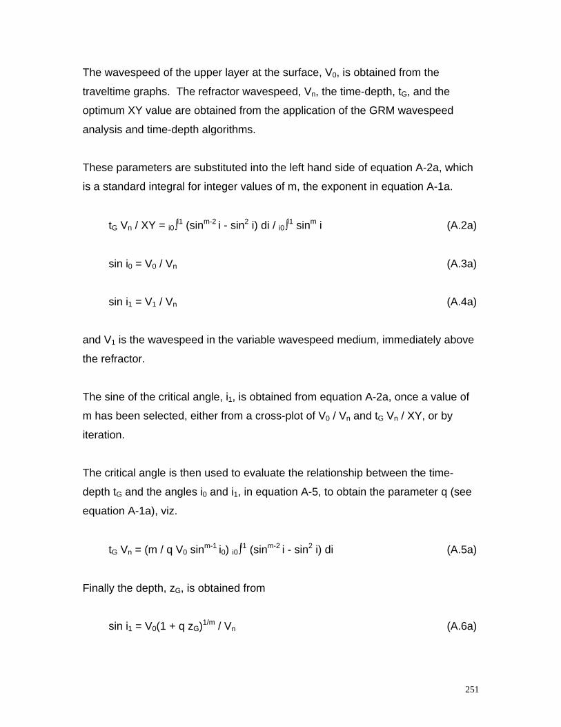
251
The wavespeed of the upper layer at the surface, V0, is obtained from the
traveltime graphs. The refractor wavespeed, Vn, the time-depth, tG, and the
optimum XY value are obtained from the application of the GRM wavespeed
analysis and time-depth algorithms.
These parameters are substituted into the left hand side of equation A-2a, which
is a standard integral for integer values of m, the exponent in equation A-1a.
tG Vn / XY = i0∫i1 (sinm-2 i - sin2 i) di / i0∫i1 sinm i (A.2a)
sin i0 = V0 / Vn (A.3a)
sin i1 = V1 / Vn (A.4a)
and V1 is the wavespeed in the variable wavespeed medium, immediately above
the refractor.
The sine of the critical angle, i1, is obtained from equation A-2a, once a value of
m has been selected, either from a cross-plot of V0 / Vn and tG Vn / XY, or by
iteration.
The critical angle is then used to evaluate the relationship between the time-
depth tG and the angles i0 and i1, in equation A-5, to obtain the parameter q (see
equation A-1a), viz.
tG Vn = (m / q V0 sinm-1 i0) i0∫i1 (sinm-2 i - sin2 i) di (A.5a)
Finally the depth, zG, is obtained from
sin i1 = V0(1 + q zG)1/m / Vn (A.6a)
252
Appendix 3
Surefcon.c
/* Copyright (c) Colorado School of Mines, 1999.*/
“
/* All rights reserved. */
/*SUCONV: $Revision: 1.12 $ ; $Date: 1996/09/05 19:24:26 $ */
"
"
#include "su.h"
"
#include "segy.h"
"
#include "header.h"
"
"
/*********************** self documentation **************************/
char *sdoc[] = {
" ",
" SUREFCON - Convolution of user-supplied Forward and Reverse ",
" refraction shots using XY trace offset in reverse shot ",
"
", surefcon <forshot sufile=revshot xy={trace offseted} >stdout ",
" ",
" Required parameters: ",
" sufile= file containing SU trace to use as reverse shot ",
253
" xy = Number of traces offseted from the 1st trace in sufile ",
" ",
" Optional parameters: ",
" none ",
" ",
" Trace header fields accessed: ns ",
" Trace header fields modified: ns ",
" ",
" Notes: It is quietly assumed that the time sampling interval on the",
" output traces is the same as that on the traces in the input files.",
" ",
" Examples: ",
" suconv<DATA sufile=DATA xy=1 | ...
","
",
" Here, the su data file, \"DATA\", convolved the nth trace by ",
"
" (n+xy)th trace in the same file ",
" ",
" ",
NULL};
/* Credits:
* CWP: Jack K. Cohen, Michel Dietrich
* UNSW: D. Palmer, K.T. LEE
*
* CAVEATS: no space-variable or time-variable capacity.
* The more than one trace allowed in sufile is the
* beginning of a hook to handle the spatially variant case.
*
* Trace header fields accessed: ns
* Trace header fields modified: ns
*/
/**************** end self doc ********************************/
segy intrace, outtrace, sutrace;
int
254
main(int argc, char **argv)
{
int nt; /* number of points on input traces */
int ntout; /* number of points on output traces */
int xy; /* the offset number for GRM */
float *forshot; /* forward shot */
int nforshot; /* length of input wavelet in samples */
cwp_String sufile; /* name of file of forward SU traces */
FILE *fp; /* ... its file pointer */
int itr; /* trace counter */
/* Initialize */
initargs(argc, argv);
requestdoc(1);
/* Get info from first trace */
if (!gettr(&intrace) ) err("can't get 1st reverse shot trace");
nt = intrace.ns;
/* Default parameters; User-defined overrides */
if (!getparint("xy", &xy) ) xy = 0;
/* Check xy values */
if (xy < 0) err("xy=%d should be positive", xy);
if (!getparstring("sufile", &sufile)) {
err("must specify sufile= desired forward shot");
} else {
/* Get parameters and set up forshot array */
fp = efopen(sufile, "r");
for (itr = 0; itr <= xy; ++itr) {
if (!fgettr(fp, &sutrace) ) {
err("can't get 1st requested forward trace");
};
};
nforshot = sutrace.ns;
255
forshot = ealloc1float(nforshot);
/* Set output trace length */
ntout = nt + nforshot - 1;
/* Main loop over reverse shot traces */
do {
fprintf(stderr,"rev==%d\t , for=%d\t", intrace.tracf,
sutrace.tracf);
memcpy((void *) forshot,
(const void *) sutrace.data, nforshot*FSIZE);
/* Convolve forshot with revshot trace */
conv(nforshot, 0, forshot,
nt, 0, intrace.data,
ntout, 0, outtrace.data);
/* Output convolveed trace */
memcpy((void *) &outtrace, (const void *) &intrace,
HDRBYTES);
outtrace.ns = ntout;
outtrace.dt = outtrace.dt/2;
/*outtrace.cdp = 2*intrace.tracf + xy;*/
fprintf(stderr,"out_cdp=%d\n", 2*intrace.tracf + xy);
puttr(&outtrace);
} while ( gettr(&intrace) && fgettr(fp, &sutrace) );
} ;
return EXIT_SUCCESS;
}
256
Appendix 4
The Effects of Spatial Sampling onRefraction Statics
Palmer, D., Goleby, B., and Drummond, B., 2000a, The effects of spatial
sampling on refraction statics: Exploration Geophysics, 31, 270-274.