
IZA DP No. 3777
Determinants of Historic and Cultural LandmarkDesignation: Why We Preserve What We Preserve
Douglas S. NoonanDouglas Krupka
DI
SC
US
SI
ON
PA
PE
R S
ER
IE
S
Forschungsinstitutzur Zukunft der ArbeitInstitute for the Studyof Labor
October 2008

Determinants of Historic and
Cultural Landmark Designation: Why We Preserve What We Preserve
Douglas S. Noonan Georgia Institute of Technology
Douglas Krupka
IZA
Discussion Paper No. 3777 October 2008
IZA
P.O. Box 7240 53072 Bonn
Germany
Phone: +49-228-3894-0 Fax: +49-228-3894-180
E-mail: [email protected]
Any opinions expressed here are those of the author(s) and not those of IZA. Research published in this series may include views on policy, but the institute itself takes no institutional policy positions. The Institute for the Study of Labor (IZA) in Bonn is a local and virtual international research center and a place of communication between science, politics and business. IZA is an independent nonprofit organization supported by Deutsche Post World Net. The center is associated with the University of Bonn and offers a stimulating research environment through its international network, workshops and conferences, data service, project support, research visits and doctoral program. IZA engages in (i) original and internationally competitive research in all fields of labor economics, (ii) development of policy concepts, and (iii) dissemination of research results and concepts to the interested public. IZA Discussion Papers often represent preliminary work and are circulated to encourage discussion. Citation of such a paper should account for its provisional character. A revised version may be available directly from the author.

IZA Discussion Paper No. 3777 October 2008
ABSTRACT
Determinants of Historic and Cultural Landmark Designation: Why We Preserve What We Preserve*
There is much interest among cultural economists in assessing the effects of heritage preservation policies. There has been less interest in modeling the policy choices made in historic and cultural landmark preservation. This paper builds an economic model of a landmark designation that highlights the tensions between the interests of owners of cultural amenities and the interests of the neighboring community. We perform empirical tests by estimating a discrete choice model for landmark preservation using data from Chicago, combining the Chicago Historical Resources Survey of over 17,000 historic structures with property sales, Census, and other geographic data. The data allow us to explain why some properties were designated landmarks (or landmark districts) and others were not. The results identify the influence of property characteristics, local socio-economic factors, and measures of historic and cultural quality. The results emphasize the political economy of implementing preservation policies. JEL Classification: Z1, R52, D78 Keywords: heritage preservation policy, landmark designation Corresponding author: Douglas S. Noonan School of Public Policy Georgia Institute of Technology Atlanta, GA 30332-0345 USA Email: [email protected]
* This document contains demographic data from Geolytics, Inc East Brunswick, NJ.

I. Introduction
Since the 1960s, historical preservation policies have been used to protect local cultural
landmarks, as well as to promote local development. Landmark designation by local
governments may have various effects on the value of historical and cultural properties
and their neighbors. There has been some interest by academics and policy advocates in
assessing the effects of landmark designation on property values, with mixed results.
There has been very little interest in modeling the designation process itself. Without
understanding how designation occurs, making causal inferences about historic and
cultural preservation policies will be problematic. This paper develops a theoretical
model of landmark designation and explores empirical determinants of designation using
a combination of several rich datasets for buildings in Chicago.
The theoretical model highlights several key aspects of historic landmark
preservation policies. The model highlights the costs and benefits of designation, the
choice among alternative policy instruments, and how political economic considerations
affect the preservation decisions of program administrators. The theoretical model gives
rise to several predictions that are empirically tested. We develop a discrete choice
model for landmark designation which identifies the determinants of designation.
Among the determinants tested are a rich array of property characteristics, local
economic and demographic characteristics, and other geographic variables for the
property. The model is applied to data for Chicago, combining the Chicago Historical
Resources Survey of over 17,000 historic and architecturally noteworthy structures in the
city with Multiple Listing Service sales data for over 70,000 attached-home properties in
the city during the 1990s. The data allow us to explain why some properties were

designated landmarks (or landmark districts) and others were not. This enables us to
better understand the forces that lead to historic preservation and local economic
development, as well as understand the biases in causal inferences about the price effects
of historic designation.
The rest of the paper is organized as follows. Section II discusses the relevant
literatures and policy background. A simple, general theory of the regulation decision is
developed in the third section, while a fourth section relates the theory to the empirical
analysis and describes the data we use. Section V presents the results of the empirical
analysis, focusing on the policy choice of the historical regulator and the robustness of
these results to various changes in the model or sample. A final section concludes.
II. Literature review and policy background
Heritage preservation efforts take many forms. Sometimes the efforts include public or
private ownership and a choice to maintain and preserve the resource. More indirect
efforts include providing incentives to others for their preservation activities. This might
include sponsorship or underwriting of an activity (e.g., performing some traditional rite,
maintaining an aging structure) by private or public funds. Schuster (2002) calls
attention to a suite of historic preservation policy tools that he refers to as list-based
policies. These include listing, registering, scheduling, and other forms of designations in
countless other national and local heritage preservation lists.
Among Schuster’s many interesting observations about list-based policies, a few
merit emphasis here. First, lists can serve their preservation ends by many means in
various contexts. This includes drawing attention to resources, certification, and enabling

eligibility for other policy interventions. This latter set of implications of listing can
involve positive or negative incentives (sometimes automatic, sometimes contingent on a
competitive application), different regulatory treatment, or other procedural
considerations –the origins and implementation of which are often de-coupled from the
agency or policy process that makes the list in the first place. Second, these lists of
heritage resources are large and growing worldwide. In his 2002 paper, Schuster gives
examples from France (with 15,000 listed monuments and 31,000 registered
monuments), the United Kingdom (with 528,383 listed buildings and over 10,000
conservation areas), United States (with over 1 million historic buildings and 2,300
National Historic Landmarks), and UNESCO’s World Heritage List (with 721 sites in
2001 and now boasts 851 properties). There is much concern about the designation
process itself, the criteria for listing, and the possibility of congestion or crowding-out on
the list. Understanding the impacts of historic designation policies presents an important
challenge given the scope of these lists and numerous governing authorities (e.g., the U.S.
alone hosts over 2,000 local historic district commissions).
Scholarly research on historic designations remains fairly limited, although the
collection of property price studies has grown. Using the policy’s effects on property
prices as a prominent indicator of value, several studies have explored the effects of
historical quality and local and national historic designation programs. Readers are
pointed to an extensive literature review by Mason (2005) and a somewhat dated Listokin
and Lahr (1997) report. More recently, studies by Coulson and Leichenko (2004),
Coulson and Lahr (2005), and Cyrenne et al. (2006), add to this growing literature.
Recently, Noonan (2007) provides a study of Chicago’s landmarks program, the focus of
this research. The broader literature on the economics of historic preservation features
widely varying research quality coupled with a fairly narrow focus on price effects.
Surprisingly, perhaps, little or no attention has been paid to the “supply effects” or impact
of these policies on actual conservation or preservation. The attention paid to “own-
price” effects of designation has struggled to resolve or even address important issues of
measurement (e.g., use of appraisal data, use of neighborhood aggregates) and
identification (e.g., is designation exogenous, is preexisting historical quality captured).
The academic literature recognizes some of these problems and, especially, the likely
heterogeneity across jurisdictions. While discussions of historic designation policies
often reference asymmetric information and the importance of “certification” (e.g.,
Schuster 2002), a theoretical model has yet to be applied and empirical evidence of this
effect remains elusive. Moreover, analysts have suggested that historic preservation may
benefit neighborhoods by both catalyzing revitalization of neighboring areas (e.g.,
Coulson and Leichenko 2001, Listokin, Listokin, and Lahr 1998) and stabilizing
neighborhoods thus reducing investment risks. Little direct evidence of these effects has
been offered, although Noonan (2007) does show in his repeat-sales data that housing
units in landmark buildings are actually more likely to be sold multiple times in the 1990s
than comparable units.
To date, however, very little has been said about the determinants of designation
in the first instance – and even less has been done to empirically describe why we
preserve what is preserved. Accordingly, efforts to measure or assess causal impacts of
these heritage preservation policies remain unconvincing. This paper seeks to remedy
this oversight.

III. Theoretical Model
We imagine a historic preservation regulator maximizing his administrative utility
function with respect to the restrictiveness of his preservation interventions, r, which we
model as positive and continuous.1 The regulator has direct preferences over r and the
utilities of the property owner (P) and of other affected stakeholders or neighbors (N).
Thus, the administrator will choose the restrictiveness of his intervention into the
property market (his preservation policy) in order to maximize:
1) , ( ) ( ) ( )( ); ; , ;u r z U P r z N r z r z= , ;
where UN, UP > 0 and Ur < 0. The regulator’s utility is rising in the welfare of the
(regulated) property owner and in the welfare of the neighbors. This is the case because
he cares about high property values or because residents apply political and
administrative pressure on the administrator to increase their own utility. The
administrator balances the property owners and neighbors’ opposing interests in
restrictiveness. Property owners prefer to have fewer restrictions (Pr < 0) in order to
preserve the option of redevelopment. Neighbors favor more restrictions (Nr > 0),
assuming those restrictions do not restrict their own options. Neighbors are expected to
value restrictions on their neighbors because this reduces the risk of attractive properties
being redeveloped in undesirable ways. The direct preferences over the restrictiveness
arise from administrative costs of the program such as the costs of monitoring and
1 Although preservation of buildings or other structures is the primary focus of this paper, the model can be readily extended to preservation of other heritage resources, such as artwork or cultural landscapes. The core idea – that a regulator balances interests of the owners (who enjoy options to transform or dispose of the resource) and some external constituency who receives a positive externality from that resource – holds across a variety of cultural applications.
enforcing compliance. The first-order direct and indirect preferences over the exogenous
factors2 z will not be important to the model because they are not choice variables for the
administrator. The role of the second-order effects will become important below.
The administrator optimizes on a property-by-property basis by setting the
marginal utility of restrictiveness to zero:
2) . ( , , , ) 0P r N r rF r x y z U P U N U= + + =
For interior solutions, equation 2 holds at the optimum and thus implicitly defines r* as a
function of z. We also assume that the second-order condition (that Fr < 0) is satisfied so
that equation 2 implicitly defines r*(z) as the utility-maximizing level of restrictiveness.
Using the implicit function rule we can derive the partial effects of any of these
exogenous characteristics on the optimal level of restriction, r*:
3) ( )*
/P rz N rz rzr U P U N U Dz
∂= − + +
∂
where < 0 is implied by the assumption that the second-
order condition is satisfied.
r P rr N rr rrD F U P U N U= = + +
3
Equation 3 helps us understand how independent variation in a host of exogenous
neighborhood or property characteristics will affect the optimal level of restrictiveness.
In general, such a factor will increase the level of restrictiveness whenever
P rz N rz rzU P U N U+ + > 0, which means that it increases the marginal utility of
restrictiveness. The term is basically the sum of the effect of z on the marginal utilities of 2 These exogenous factors will include characteristics of individual properties, owners, or neighborhoods and will be discussed below. The direct and indirect preferences will vary depending on which exogenous factor is considered.
3 A sufficient condition for this condition to hold are that administrative costs increase more-than-linearly, that the added benefit to neighbors is decreasing in restrictiveness, and that the costs imposed on property owners by restrictions increases about linearly.
each stakeholder, weighted by the administrator’s weight of each stakeholder’s utility.
To flesh out this condition, we examine some examples of such variables.
Some characteristics of the property affect only the property owners. Such a
characteristic might be the value of a property after potential redevelopment. This
increases the owner’s utility by increasing the value of the property, but should not affect
the neighbors. Owners of structures with more redevelopment-related option value will
likely have their utility more adversely affected by additional restrictions (UPPrz < 0),
while this factor will likely have little effect on the marginal utility of restrictions to the
administrator. Thus, the model predicts that factors making potential redevelopment
more profitable will decrease the optimal level of restrictions.
Some factors will affect neighbors but not property owners. One such element of
z is the negative externalities that would be created if the structure was redeveloped. For
instance, if the likely post-redevelopment use of a historic apartment building is a gas
station, neighbors will likely value restrictions even more than if the post-redevelopment
use is a library or housing. If z is “negative externality associated with redevelopment,”
UNNrz > 0, while the other cross-partials will be near zero. Thus, the model predicts that
restrictions will increase when the future use of properties will bring more negative
externalities.
Above, we mentioned the historic nature of the property might both decrease the
property owner’s utility (outdated structural characteristics, Pz < 0) but increase
neighbors’ utility (rare architectural style, Nz > 0). Higher restrictions will tend to make
living in a historic property worse (Prz < 0, because modifications will be more difficult),
but also make its external effect on neighbors more positive (Nrz ≥ 0, because reduced
uncertainty about the persistence of the positive externalities will benefit risk-averse
neighbors). The effect on the costs of regulating will be indeterminate because the
outdated but historical nature of the structure will encourage both the property owner and
the neighbors to lobby the administrator for their preferred restrictions, while there is
nothing inherent about the historic nature that makes the restrictions harder to administer
( 0 ). From this, the effect of historical quality on protection or preservation is
ambiguous.
rzU ≈
Factors other than the property’s own historic qualities might make the difference.
For a given level of historic value, the preservation of a property in a more historic
neighborhood (with many historic properties) might not add very much to neighbors’
utility (i.e., Nz and Nrz will be smaller in more historic neighborhoods), and less
regulation will be expected. If the historic property stands out, say, because it is old
compared to the rest of the neighborhood, the opposite holds, and regulation might be
more stringent. Similarly, for a given amount of historic significance, a more culturally
significant structure will have higher optimal restrictions. Higher incomes might increase
people’s valuation of certainty over future flows of historic externalities or increase the
ability of neighbors to decrease the marginal disutility of adding restrictions (increase
Nrz).
Two common features of historic preservation policy are that regulation is limited
to a few discrete choices, and that protected properties can be bundled together into
landmark districts. Our model allows for such group designations, but this is a detail
away from which we have abstracted considerably. If an administrator can only make
group designation decisions, the optimization problem above is subtly altered. Landmark

districts offer administrators another choice in the policy instrument with which they
approach the preservation decision. For group or district designations, the neighbors and
the property owners are groups which substantially overlap, suggesting that the effects of
income and other demographic factors on the optimal restrictiveness could differ
markedly from individual property regulations. Similarly, the effect of the nearness of
additional historic properties in the vicinity (which lowered the level of individual
restrictions) might increase the level of group restrictions since imposing group
restrictions might have lower marginal costs per unit to the administrator. Because the
determinants of group designation and individual designation can differ so markedly, the
optimal level of restrictions will also differ depending on the type of designation. Thus,
for a given structure, there will be one optimal level of restrictions for the case of
individual building designations, rb*( z), and a different level of restrictiveness for district
designations, rd*( z).
Our model adjusts readily to the mostly discrete nature of preservation policy. In
the empirical section to follow, the continuous r* terms from the model become latent
variables in logit regressions, so that designation will occur whenever r* exceeds some
cut-off value. Faced with three regulation possibilities (leave the property alone,
designate it as part of a district, or designate it as an individual building), the
administrator will choose the one that yields the highest utility. The two types of
designations also confer eligibility for different incentive programs (such property or
income tax reductions, zoning variances and technical assistance). Thus, our multinomial
logit analysis will take the district/individual distinction as the primary discrete choice
faced by administrators.

IV. Data and empirical model
The empirical model
In the theoretical model above, the utility the administrator receives from
regulating any structure, i, according to the optimal regulation for policy instrument c is
given by:
4) ( )( )*ic c i icu U r z ε= + ,
where εic is a random error term following a type-I extreme value distribution and c can
be either no regulation (n), district designation (d) or building designation (b). For our
statistical analysis, we assume that
5) ( )( )*0c i c zc i iU r z z cβ β ε= + + .
If the administrator always chooses the option yielding the highest utility, the probability
that he chooses any given preservation policy, pi for a given structure is given by:
6) 0
0Pr( )
1
c zc i ic
c zc i ic
z
i z
c
ep ce
β β ε
β β ε
+ +
+ += =+∑
for c=d, b.4 We estimate these empirical equations via maximum likelihood.
We also perform an analysis of the district designation decisions using standard
logistic regressions. Where:
7) Pr (c=d | z) = Pr (rd*(z) > 0 | z) = Pr (β0+ βzz+ ε2 > 0| z)
4 For policy instrument c = n, or no regulation, the probability of being unregulated is set to be equal to equation 6 with the numerator replaced with 1.

These models are important in terms of checking the robustness of our results, and
interesting in their own right. Because of the rarity of individual designations, we are not
able to control for large amounts of structural and neighbor characteristics in our
multinomial logit analysis. Thus, we assess the robustness of the coefficients in the
district-only models, and discuss them in light of the results from the multinomial logit
models.
The data
The empirical analysis combines many data sources. The City of Chicago’s
Landmarks Division in its Department of Planning and Development provides
information on the landmarks (City of Chicago 2004). Information such as the addresses,
dates of construction and designation, architect and architectural style, and historic
themes are available for the 217 individual landmarks and 43 historic districts
(comprising over 4,500 properties) in the city. These data provide us with the dependent
variables of our empirical analysis, which is designation during the 1990’s.
Combined with the official landmarks data is the Chicago Historical Resources
Survey (CHRS). Starting in 1983, historians from the Landmarks Commission
inventoried the half million structures in Chicago’s city limits (Commission on Chicago
Landmarks 1996). Commission on Chicago Landmarks (1996) describes the
methodology in greater detail. Ultimately, the fieldwork obtained detailed information
from a final sample of 17,366 historically and/or culturally significant properties. The
CHRS data contains information on addresses, architects, significance and maintenance,
and construction dates (http://www.cityofchicago.org/Landmarks/CHRS.html). The

analysis also uses a variety of other geographic data for the city including Chicago’s
community areas and Census TIGER files. To link properties to their block-group level
Census variables, the Geolytics™ dataset is employed to produce boundary-constant
neighborhood demographics for 1980-2000.
To examine which properties are more likely to be designated as landmarks,
ideally data on the population or a random sample of Chicago properties would be used.
No such dataset is available, however. Timely citywide property inventories with
sufficient detail are generally not maintained. Lacking an available and ideal sample of
data, this paper examines two different samples of Chicago properties. The first is the
sample of properties in the CHRS mentioned above. This sample might be thought of as
a deliberate oversample of old, historically or culturally significant, and likely-to-become
designated properties. The second is a sample of all single-family attached houses (e.g.,
condos, townhomes) that were sold via the Multiple Listing Service (MLS) from1990-
2000.
A few differences between the CHRS and MLS datasets should be noted. The
CHRS functions like cross-sectional inventory of historic properties in the city because
the date each observation was taken is unknown. The MLS data, on the other hand, offer
true time-series data on property sales over the course of a decade. This analysis
establishes a baseline in 1990, exactly the start of the MLS data range and near to the end
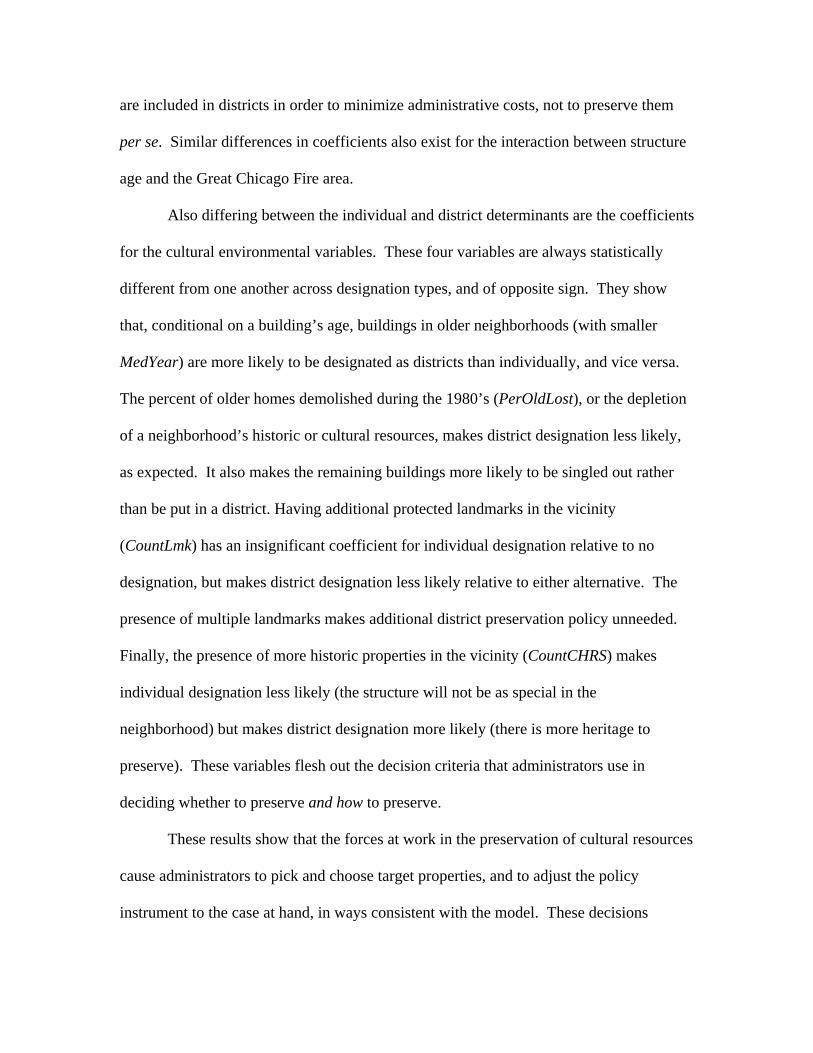
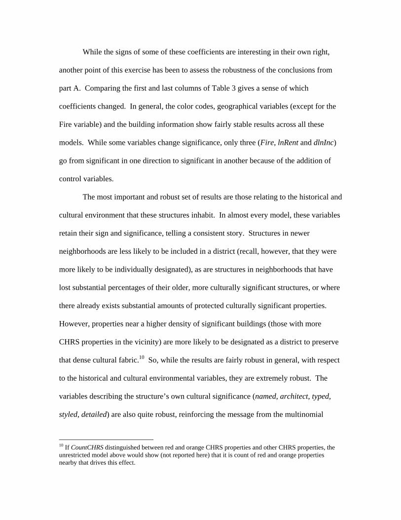
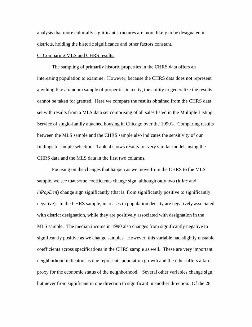
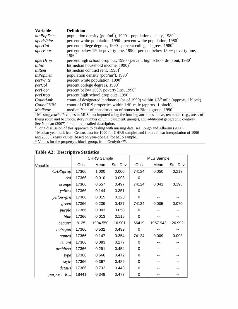
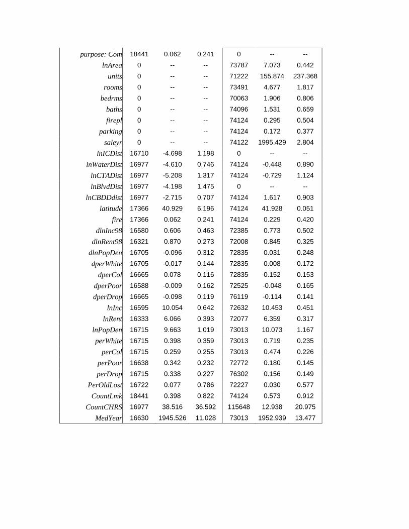
of the CHRS surveying effort.5 Table A1 provides definitions for variables used in the
5 Because of data limitations, we assume that CHRS data were collected by 1990. For CHRS properties surveyed after 1990, it is possible an endogeneity or sample selection bias might occur. The dependent variable (post-1990 designation status) might influence the independent variables from the CHRS dataset or even the likelihood of inclusion in the CHRS. If designated properties are more likely to be included, then inferences drawn from estimates using this sample may not be valid for the broader population of structures. For instance, oversampling designated-but-low-quality buildings might artificially lower the estimated effect of quality of designation. If designation status affects how surveyors recorded property

analysis and indicates from which datasets they derive. Summary statistics for the two
samples of properties (CHRS and MLS) can be seen in Table A2.
In the theoretical model, all independent variables are collapsed into one variable,
z. The discussion of the model considered various interpretations of that model,
including the historic nature of the structure, its cultural significance, its historic or
cultural built environment and the income and other demographic characteristics of its
neighborhood. The CHRS includes a set of color codes which contain some information
on the historic or cultural significance. Our primary measure of historical significance is
simply the year the structure’s construction was begun (begun), along with an interaction
of this variable with it location within the zone affect by the Great Chicago Fire of 1871
(FireBegun).6 We also use a set of geographic variables to control for location in the
Great Fire zone and for distance to the center of downtown Chicago, to water features, to
industrial corridors, and to one of Chicago’s historic boulevards. The latitude of the
structure controls for location in the north side of the city. Other controls for building
characteristics include the purpose of the structure (residential, commercial or other).
Whether the CHRS property had a known tenant at the time of the survey (tenant) is also
included as a proxy for lobbying interest and capacity. Actively used buildings may be
better able to resist designation than vacant ones, just as purpose might indicate different
owner interests.
information – or affected the building attributes directly – then classic endogeneity occurs. For example, designated buildings might receive higher quality scores than they would have without the prestige of designation, biasing upwards the estimated effect of quality on designation.
6 The Great Chicago Fire of 1871 devastated much of the city core at the time, forcing a virtual rebuilding of this portion of the city. This puts an upper limit on building age in that area. Because the begun variable is missing for many observations, begun is coded with a 0 for all missing observations and a dummy variable (nobegun) is included to capture the mean effect of those buildings with missing begin values. See Longo and Alberini (2006) for an application of this approach.

Our proxies of cultural significance in the CHRS data are a set of dummy
variables describing the extent to which information about the structure was known.
These included dummy variables for whether the building was named (e.g., “the Robie
House”), whether the architect was known, whether the building was assigned a specific
type, or details, or described as an example of a particular architectural style. The historic
or cultural environment is measured by a set of variables for the median year of
construction in the structure’s census block group (MedYear), the stock of pre-1990
designated landmarks in the block group (CountLmk), the percentage of the 1980 stock of
pre-war housing that was demolished during the 1980’s (PerOldLost) and the number of
CHRS properties within a half mile of the structure (CountCHRS).
Finally, we have a set of neighborhood demographic variables. These include the
average income (lnInc), rent (lnRent) and the population density (lnPopDen) in our most
basic models. In more fully specified models, we have included variables for the percent
of the population with college degrees (perCol), the percent without high school degrees
(perDrop), the percent of the population that is non-Hispanic, white (perWhite), and the
percent of the households with incomes below 150% of the official poverty line
(perPoor).
Many of these variables are not available in the MLS data, except for structures
that happen to be in both data sets. The MLS does offer a host of other structure
variables which we use, including the square footage (Area), number of units in the
building (units), the number of rooms, bedrooms and bathrooms (rooms, bedrms, and
baths, respectively), the presence of a fireplace (firepl) or parking spot (parking) and the
year of sale (saleyr). When analyzing the MLS data, we also include controls for

whether the property was deemed culturally significant enough to be included in the
CHRS and some of the CHRS variables.
V. Results
Table 1 presents the averages of the various outcome variables for the two data
sets to give a sense of the extent of the programs. We see that in both samples post-1990
landmark designations are relatively rare. Such late designations make up only five
percent of the CHRS sample (compared to 14% pre-1990 designations) and only about
one percent of the MLS sample (compared to about 2.5% for pre-1990 designations). A
much greater number of landmarks were designated before 1990. About five percent of
the MLS sample is also in the CHRS sample, comprising about 3,600 observations.
Among these CHRS observations in the MLS data set, nearly 20 percent are in landmark
districts, and nearly seven percent were included in districts after 1990.
Table 1: Landmark status in the two data sets. CHRS MLS Prop. Freq. Prop. Freq. All Landmarks 0.1994 3462 CHRS Property 0.0504 3603 Pre-1990 0.1420 2466 District Ever 0.0353 2528 Post-1990 0.0574 996 District Post-1990 0.0088 627 Post-1990 Districts 0.0569 966 Post-1990 Individual 0.0018 30 Obs 1.0000 17366 Obs 1.0000 71534 The rest of this empirical section is split into three parts. First, using the CHRS
data we present the "policy choice" model, where administrators choose whether to
regulate, and how. In part B, we add additional variables to the district model to assess
the robustness of the estimated coefficients to the inclusion of additional explanatory
variable. Part C compares the estimated coefficients from the CHRS district model to a

comparable set of results using the MLS data, and adds some additional variables to the
models using MLS data to assess robustness to included variables.
A. Policy Choice
Table 2 reports the coefficients from the multinomial logit estimation of a model
where administrators can assign a structure either no additional restriction (beyond city
zoning and state and federal historical protections), include it in a district, or single out
the structure for individual designation.7 The top panel of Table 2 reports the coefficients
for the individual designations (relative to no designation at all), and the bottom panel
reports coefficients for district designations (relative to no designation at all). The
Model 1 in Table 2 starts with a basic specification. Model 2 adds prior changes in
neighborhood demographics in the middle column. A parsimonious model is specified
because of the rarity of the ‘individual designation’ policy choice.
Several variables have qualitatively similar coefficients across the two types of
designation. These include the historical color codes (-),the variables for whether the
structure was named (+) or had a tenant (-), neighborhood rent levels (+), population
density (+), whether the structure was in the zone affected by the Great Chicago Fire of
1871 (+) and whether the structure was a residential property (-).8 That historical quality
appears negatively related to the likelihood of historic designation is one of the more
remarkable results for this analysis. The interpretation of the color code results are
discussed in more detail below. There are several coefficients that differ between
7 Strictly speaking, the model predicts whether structures are not designated, designated in a district, or individually designated at some point after 1990. Because a structure that was designated prior to 1990 cannot, in general, be re-designated during the 1990’s, we drop these structures form the data set in all the regressions reported here.
8 Some of these coefficients are insignificant for one of the designation types and not statistically different from one another at conventional levels. In those cases, we report the sign of the significant coefficient.

designation types. Some of the less interesting ones include the distance to the center of
downtown and whether the property had a commercial use (both are insignificant for
individual designations, significant and negative for districts).
Some important variables’ coefficients differ markedly by designation type. The
negative coefficient on neighborhood income for district designation (relative to no
designation) is significantly different from the smaller, insignificant negative coefficient
for individual designation. If historic and cultural preservation is a normal good, these
results are somewhat surprising. They suggest that individuals in high income
neighborhoods do not want the restrictions placed on their homes, and have the incentive
and wherewithal to prevent such designations. The much smaller coefficient for income
for the individual designation choice suggests that this incentive does not prevent the
restrictions from being placed on their neighbor through individual designation, but
neighborhood income does matter when the restrictions threaten their own options
through district designations. Similarly, increases in rents over the 1980’s have
significantly different effects in the two models, with negative effects on individual
designation and positive or insignificant effects on district inclusion.
Another interesting difference in determinants is that of the date at which
construction of the structure was begun. Newer structures are significantly less likely to
be individually designated (relative to no designation at all), as expected. The effect of
age on inclusion in a landmark district (rather than not designated at all) is non-existent.
The difference in the coefficients is significant in Model 2. That individual structural age
is important in determining individual designation but unimportant in determining
inclusion in a district squares with intuition and the model: many non-historic properties
are included in districts in order to minimize administrative costs, not to preserve them
per se. Similar differences in coefficients also exist for the interaction between structure
age and the Great Chicago Fire area.
Also differing between the individual and district determinants are the coefficients
for the cultural environmental variables. These four variables are always statistically
different from one another across designation types, and of opposite sign. They show
that, conditional on a building’s age, buildings in older neighborhoods (with smaller
MedYear) are more likely to be designated as districts than individually, and vice versa.
The percent of older homes demolished during the 1980’s (PerOldLost), or the depletion
of a neighborhood’s historic or cultural resources, makes district designation less likely,
as expected. It also makes the remaining buildings more likely to be singled out rather
than be put in a district. Having additional protected landmarks in the vicinity
(CountLmk) has an insignificant coefficient for individual designation relative to no
designation, but makes district designation less likely relative to either alternative. The
presence of multiple landmarks makes additional district preservation policy unneeded.
Finally, the presence of more historic properties in the vicinity (CountCHRS) makes
individual designation less likely (the structure will not be as special in the
neighborhood) but makes district designation more likely (there is more heritage to
preserve). These variables flesh out the decision criteria that administrators use in
deciding whether to preserve and how to preserve.
These results show that the forces at work in the preservation of cultural resources
cause administrators to pick and choose target properties, and to adjust the policy
instrument to the case at hand, in ways consistent with the model. These decisions

depend on the neighborhood context (demographic, economic and cultural) as well as the
properties of the individual structure. Individual designations tend to happen to older
properties in less historic neighborhoods, while districts tend to be in poorer
neighborhoods with more historical resources.
B. District models.
Because of the small number of individual designations after 1990, the
multinomial logit analysis above restricts itself to a limited set of explanatory variables.
We now turn to an analysis solely of the choice to designate a property in a district or not.
The greater frequency with which properties become included in a district allows us to
include a larger set of explanatory variables, examine these new variables’ coefficients
and assess how stable the relationships described in part A are in the face of additional
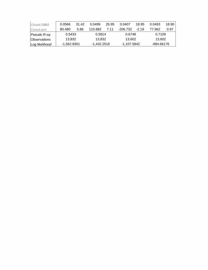
controls. Table 3 presents these results. The first column of results presents coefficients
of a logit regression with additional color codes added, and shows that there are no
qualitative changes from the multinomial logit models in Table 2. The next column
includes some additional building details, while a third incorporates more geographic
information. The rightmost column of results adds additional demographic and
demographic trend variables. The inclusion of these variables makes some of the
already-included variables’ coefficients change sign.
The coefficients of added building characteristics generally show that having
more information about a building makes it more likely to be designated. These building
characteristics are our main proxy of cultural significance, so these results suggest (along
with those results in table 2) that more culturally significant buildings (e.g., greater fame
or notoriety of the building or its architect, representativeness of its architectural style)

are more likely to be designated, as the theory predicts. Adding these variables to the
model causes the named and Fire coefficients to become insignificant, and the residential
use dummy variable coefficient to become significantly negative. Also, including these
cultural variables makes the begun variable become significantly negative. The
construction date’s insignificance in the model with fewer cultural significance measures
shows that the interplay between a building’s cultural and historical significance is
important. Landmark designations in Chicago appear to be able more than just history –
cultural dimensions matter as well, and the effects of one may mask the other in an
improperly specified model.
Adding the geographic information shows that a more northern location is
associated with a greater likelihood of district designation, as does being located further
away from industrial corridors or bodies of water (e.g., Lake Michigan, Chicago River).
Adding these variables causes the Fire dummy variable to become significantly negative
along with the dummy for having no information about construction dates, but the
residential use variable goes back to positive. Furthermore, these geographic variables
drive the 1990 rental rates coefficient and the percent of lost old residences coefficient
into insignificance. It would be difficult to generalize much from the effect of these
geographic controls on the other variables. The geographic coefficients as well as their
effects on the other coefficients says more about the specific historical development of
the city of Chicago than anything else.
Finally, the additional demographic information yields a positive association with
the percent white in 1990 and the 1980-1990 change in the percent college educated. The
percent college educated in 1990, the changes in the poverty rate and percent white over

the 1980’s are all associated with lower probability of being designated. Adding these
variables has big effects on the previously-included demographic variables, as might be
expected. When the new demographic variables are added, 1990 rental rates and the
change in neighborhood income from 1980-1990 become significant and negative, while
1990 neighborhood income levels becomes insignificant, as does the dummy variable for
whether the CHRS data set included information on the style of the structure. However,
the percentage of older homes demolished during the 1980’s becomes significantly
negative again, as in previous models.
The three demographic variables which change signs in the presence of the new
demographic controls (lnRent, lnInc and dlnInc) might be expected to change sign in the
presence of the additional demographic controls. For instance, while income changes
sign from negative to positive, it is only in the presence of the strong negative coefficient
of the college variable that this occurs. The same is true for the switch of the coefficient
on income changes and the sign of the coefficient of changes in college education: the
income variable changes sign, but only in the presence of the new college variable, which
takes the sign that the income variable had in the college variable’s absence. The
interpretations loaded on the income variable in part A could thus now be leveled on a
“class” variable, as represented by the college education levels in the neighborhood, and
these results support the idea that education, class and the cultural tastes and attitudes
associated with them are more important than income per se.9
9 The connection between income and education as determinants of demand for heritage preservation, and cultural goods in general, is discussed in greater detail elsewhere (e.g., Bourdieau 1984). This is another instance of education being a better predictor of cultural demand than income (e.g., Heilbrun and Gray 2001, Whitehead and Finney 2003, Alberini and Longo 2006).
While the signs of some of these coefficients are interesting in their own right,
another point of this exercise has been to assess the robustness of the conclusions from
part A. Comparing the first and last columns of Table 3 gives a sense of which
coefficients changed. In general, the color codes, geographical variables (except for the
Fire variable) and the building information show fairly stable results across all these
models. While some variables change significance, only three (Fire, lnRent and dlnInc)
go from significant in one direction to significant in another because of the addition of
control variables.
The most important and robust set of results are those relating to the historical and
cultural environment that these structures inhabit. In almost every model, these variables
retain their sign and significance, telling a consistent story. Structures in newer
neighborhoods are less likely to be included in a district (recall, however, that they were
more likely to be individually designated), as are structures in neighborhoods that have
lost substantial percentages of their older, more culturally significant structures, or where
there already exists substantial amounts of protected culturally significant properties.
However, properties near a higher density of significant buildings (those with more
CHRS properties in the vicinity) are more likely to be designated as a district to preserve
that dense cultural fabric.10 So, while the results are fairly robust in general, with respect
to the historical and cultural environmental variables, they are extremely robust. The
variables describing the structure’s own cultural significance (named, architect, typed,
styled, detailed) are also quite robust, reinforcing the message from the multinomial
10 If CountCHRS distinguished between red and orange CHRS properties and other CHRS properties, the unrestricted model above would show (not reported here) that it is count of red and orange properties nearby that drives this effect.
analysis that more culturally significant structures are more likely to be designated in
districts, holding the historic significance and other factors constant.
C. Comparing MLS and CHRS results.
The sampling of primarily historic properties in the CHRS data offers an
interesting population to examine. However, because the CHRS data does not represent
anything like a random sample of properties in a city, the ability to generalize the results
cannot be taken for granted. Here we compare the results obtained from the CHRS data
set with results from a MLS data set comprising of all sales listed in the Multiple Listing
Service of single-family attached housing in Chicago over the 1990's. Comparing results
between the MLS sample and the CHRS sample also indicates the sensitivity of our
findings to sample selection. Table 4 shows results for very similar models using the
CHRS data and the MLS data in the first two columns.
Focusing on the changes that happen as we move from the CHRS to the MLS
sample, we see that some coefficients change sign, although only two (lnInc and
lnPopDen) change sign significantly (that is, from significantly positive to significantly
negative). In the CHRS sample, increases in population density are negatively associated
with district designation, while they are positively associated with designation in the
MLS sample. The median income in 1990 also changes from significantly negative to
significantly positive as we change samples. However, this variable had slightly unstable
coefficients across specifications in the CHRS sample as well. These are very important
neighborhood indicators as one represents population growth and the other offers a fair
proxy for the economic status of the neighborhood. Several other variables change sign,
but never from significant in one direction to significant in another direction. Of the 28

variables included in the equation, only 7 show instability, and 21 retain the same sign
and significance regardless of the sample. Throughout the paper, we have focused on the
coefficients on the variables measuring the historical and cultural environment of the
structure. One of these variables (PerOldLost) becomes insignificant in the MLS
sample.11 The rest of the interesting historical environment variables are consistent with
what came before.
The last two columns of results in Table 4 use the MLS sample, but add control
variables. We first add a number of individual structural characteristics available in the
MLS data, but not in the CHRS. Of these, the living area is positively associated with
district designation while the number of bathrooms, access to a parking space, and the
year of sale are negatively associated with district designation. The last of these
coefficients suggests that attached housing sales are increasingly in non-landmark
districts over the 1990s. The size of the building (units) is inversely related to the
likelihood of district designation throughout its range in both the last two columns. The
addition of the unit characteristics also drives the CountLmk coefficient insignificant,
although it retains its negative sign. As with the change in significance of PerOldLost, it
is important to remember that this coefficient pertains holding the median age of
neighboring structures and the number of nearby CHRS properties constant.
The negative coefficient for certain color codes (e.g., orange, red) remains in the
MLS sample. This unexpected result suggests several possible explanations. First, most
11 Interestingly, the percentage of old housing lost during the 1990s is positive and significant when included in a similar regression. Because this variable is endogenous, we do not report any such regressions here. Its significance could be interpreted cynically (that preservation policies lead owners to demolish houses). Another interpretation is that high rates of demolition increase the demand for preservation by neighbors, leading administrators to preserve areas “threatened” by development. Much hinges on the timing of the preservation and the demolition, which we cannot address here.

of the most significant heritage resources were already designated landmarks by 1990.
The “red” or “orange” properties not already designated in the first 22 years of the
program likely remain undesignated for some other reason. It might be some
unobservable (e.g., existing easements, politically powerful owners) that either makes
their designation too costly or redundant. After the administrator has already “cherry-
picked”, properties of less-significant color codes, which lack these unobservables,
appear more likely to become designated. Second, at least for the properties not yet
designated by 1990, the coding criteria in the CHRS apparently diverge substantially
from the many factors (e.g., history, culture, economic development, art, aesthetics)
considered by Landmarks Commission in Chicago (2007). The CHRS measure for
quality need not be the same as subsequently used by the administrator. Third, and
related to the first two, is that the effects in Tables 2 – 4 are conditional on other control
variables. For CHRS structures, individual designations are significantly and positively
(unconditionally) correlated with red and yellow properties, significantly negatively
correlated with green, and not significantly correlated with orange (the modal category).
Finally, for codes other than red or orange, the codes partly reflect modifications that
have occurred to the property. The historic-but-modified property may be more likely
than historic-and-authentic to merit designation of any sort because the modification may
signal that the remaining heritage resource is at greater risk (raising Nr) or may signal that
the owner has already made the desired modernization (lowering Pr).
In general, moving form the CHRS to the MLS does not create large changes in
the estimated coefficients. Comparing the first column of results in Table 4 with the last,
we see that of the 28 common coefficients between the MLS and CHRS datasets, only

nine change, and only two change from significant in one direction to significant in
another. While two of our four historical and cultural environmental variables become
insignificant, they retain their sign. Furthermore, the proxies for historic value (the color
codes and begun) are generally robust, as is our proxy for cultural significance (named,
although it is important to keep in mind that this variable depends on MLS observations
that overlap with the CHRS dataset, so its consistency should not be surprising). All in
all, the results paint a broadly consistent picture of the designation process across
specifications and across samples.
VI. Conclusions
This paper endeavors to shed light on the process of historical and heritage preservation,
using the case of Chicago’s landmarks program. To that end, we develop a simple model
of administrative choice, and test that model on two datasets. We find sensible patterns
in the data, both in terms of the kinds of properties designated and the type of designation
chosen. An implication of the model is that the presence or absence of landmarks in a
neighborhood cannot be taken as a simple proxy for demand for cultural assets. The
designation of a structure as a landmark is the result of an interplay amongst the demands
of neighbors, the resistance of owners and the administrative behavior of the regulator.
Designation choices therefore reflect more than community members’ or experts’
assesments of (architectural, historical, etc.) quality from an inventory of historical
resources. Stand-out properties in newer neighborhoods tend to be protected via single
designation, while properties in older neighborhoods tend to be protected as part of a
large district. We find evidence that being older makes a structure more likely to be

individually designated. Additional cultural significance appears to be positively
correlated with both individual designation and district or group designation. Among
historical buildings, a structure’s age is weakly related to the likelihood of inclusion in a
landmark district unless other cultural variables are controlled for. The results shed light
on the administrative decisions historical and cultural preservation regulators make, and
their selection of policy instruments in a major American city with active preservation
policy.
Further analysis of the robustness of the findings to changes in specification finds
that the results are on the whole quite robust. Unfortunately, this analysis is restricted to
the district model because of the scarcity of individual designations. Most of the
independent variables are robust to specification changes. Those describing the historical
environment of the structure are especially robust, telling a consistent story across many
specifications. Structures in older neighborhoods with fewer protections in place and
more historical resources are more likely to be protected as districts. While this may
seem intuitively obvious, the robustness of these coefficients in the district models gives
us additional confidence in the coefficients from the more parsimonious multinomial
logit models. This further highlights the choices historical preservationists face among
policy instruments and the way in which different policies are applied.
Latent in the model is a consideration of the supply of historical resources in an
area, how that supply might evolve over time, and how policy might be used to affect that
evolution. Many discussions take a static view, assuming that the supply of heritage
resources is fixed and only depletable over time. From a resource economics standpoint,
whether historical and cultural resources are renewable is a crucial distinction. Many

policies appear to cast heritage as a nonrenewable resource, making any changes to the
stock of heritage irreversible. Future economic inquiry and empirical analysis of policy
impacts would do well to view these historic preservation policies in this light and
examine how the policies are implemented as well as their broader (and possibly
unintended) consequences. It might be the case, for instance, that the threat of
preservation policies could spur owners to redevelop preemptively, as in Turnbull (2002).
Whether such effects exist, and whether preservation policies are indeed effective in
actually preserving historical resources are issues the literature has yet to take up.
This paper also assesses the usefulness of the CHRS by comparing its results with
findings from a large sample of all sales of attached homes in Chicago over the 1990s.
We find that the results from the CHRS are fairly robust, with only a few coefficients
changing signs significantly across samples. It seems that the revealed preferences for
preservation designation among the inventory of historically and culturally significant
properties in Chicago are not altogether different than the decision criteria used for a
sample of properties selected less overtly for historical significance. The combination of
the historical information with the sales information raises the possibility in future work
of examining the complicated interplay among the value of homes, their historical and
cultural significance and the positive externality they bestow upon their neighbors. As
many of the variables used in this analysis would presumably also be significant in a
hedonic price equation, they will likely not serve as valid instruments for policy choice.
However, this paper highlights the strong possibility of endogeneity bias in the estimation
of the effects of designation policy on the value of properties designated. Similar
endogeneity problems might also complicate the measurement of external effects of such

policies on neighboring properties not directly affected by the regulation. Such
endogeneity problems are extremely important since these external effects of preservation
policy are a primary justification for preservation policies. Any examination of the
effects of these policies must first be grounded in a solid understanding of the causes of
these policies.
While we find consistent and easily interpretable results for the variables
measuring the historical and cultural environment of a structure, and many of the
structure’s own characteristics, the results are less consistent with regards to some
neighborhood-level factors. Future work might fruitfully examine exactly how
neighborhood demographics and preservation policy affect one another. Whether
designation is more likely in rich or poor, growing or shrinking, expensive or affordable,
gentrifying or disintegrating neighborhoods is interesting for a variety of reasons. As
these policies restrict property owners, concerns over the economic justice of the
decisions might be raised. The causal interaction between neighborhood demographics
and preservation policy also offer a window into the decision making of preservation
program administrators, and the effects of those decisions on the neighborhoods they
regulate.
References Alberini, Anna and Alberto Longo. 2006. “Combining the Travel Cost and Contingent
Behavior Methods to Value Cultural Heritage Sites: Evidence from Armenia.” Journal of Cultural Economics 30 (4): 287-304.
Bourdieu, Pierre. 1984. Distinction. Cambridge: Harvard University Press. City of Chicago. 2004. Chicago Landmarks: General Information.
http://www.cityofchicago.org/Landmarks/GeneralInfo.html

Commission on Chicago Landmarks. 1996. Chicago Historic Resources Survey: An Inventory of Architecturally and Historically Significant Structures. Chicago: The Department.
Commission on Chicago Landmarks. 2007. Landmarks Ordinance with Rules and Regulations of the Commission on Chicago Landmarks. Chicago: City of Chicago. Retrieved April 28, 2008, from http://www.cityofchicago.org/Landmarks/pdf/Landmarks_Ordinance.pdf
Coulson, N. Edward and Mike L. Lahr. 2005. “Gracing the Land of Elvis and Beale Street: Historic Designation and Property Values in Memphis.” Real Estate Economics 33(3): 487-507.
Coulson, N. Edward and Robin M. Leichenko. 2004. “Historic Preservation and Neighbourhood Change.” Urban Studies 41(8): 1587-1600.
Coulson, N. Edward and Robin M. Leichenko. 2001. “The Internal and External Impact of Historical Designation on Property Values.” Journal of Real Estate Finance and Economics 23(1): 113-124.
Cyrenne, Philippe, Robert Fenton, and Joseph Warbanski. 2006. “Historic Buildings and Rehabilitation Expenditures: A Panel Data Approach.” Journal of Real Estate Research 28(4): 349-379.
Heilbrun, James and Charles M. Gray. 2001. The Economics of Art and Culture. New York: Cambridge University Press.
Listokin, David and Michael L. Lahr. 1997. “Economic Impacts of Historic Preservation.” New Jersey: New Jersey Historic Trust.
Listokin, David, B. Listokin, and Michael L. Lahr. 1998. “The Contributions of Historic Preservation to Housing and Economic Development.” Housing Policy Debate 9(3): 431-478.
Longo, Alberto and Anna Alberini. 2006. “What Are the Effects of Contamination Risks on Commercial and Industrial Properties? Evidence from Baltimore, Maryland.” Journal of Environmental Planning and Management 49(5): 713-737.
Mason, Randall. 2005. “Economics and Historic Preservation: A Guide and Review of the Literature.” Brookings Institution Discussion Paper, September 2005.
Metrick, Andrew and Martin L. Weitzman. 1998. “Conflicts and Choices in Biodiversity Preservation.” Journal of Economic Perspectives 12(3): 21-34.
Noonan, Douglas S. 2007. “Finding an Impact of Preservation Policies: Price Effects of Historic Landmarks on Attached Homes in Chicago, 1990-1999.” Economic Development Quarterly 21(1): 17-33.
Schuster, J. Mark. 2002. “Making a List and Checking It Twice: The List as a Tool of Historic Preservation.” (Working Paper No. 14). Chicago: The Cultural Policy Center at the University of Chicago. Retrieved April 24, 2008, from http://culturalpolicy.uchicago.edu/workingpapers/Schuster14.pdf
Turnbull, Geoffrey. 2002. “Land Development under the Threat of Taking.” Southern Economic Journal 69(2): 468-501.
Whitehead, John C. and Suzanne S. Finney. 2003. “Willingness to Pay for Submerged Maritime Cultural Resources.” Journal of Cultural Economics 27(3-4): 231-240.

Table A1: Variable Descriptions Variable Definition DB90 dummy variable taking a 1 if property is or was in a building designated a
landmark itself (non-district) after 1990 DD90 dummy variable taking a 1 if property was in a landmark district designated
after 1990 red dummy variable (CHRS code for historical or architectural significance at the
city, state, or national level) orange dummy variable (CHRS code for significance at the community level) yellow dummy variable (CHRS code for significance lacking despite good physical
integrity) yellow-grn dummy variable (CHRS code for a lack of individual significance and an
alteration like artificial siding) green dummy variable (CHRS code for over 10% alteration from the original
appearance) purple dummy variable (CHRS code for no significance and extensive alterations) blue dummy variable (CHRS code for properties built after 1940, indicates the
structure was too recent for evaluation) begun CHRS sample: year construction began (missing values replaced with a ‘0’)
MLS sample: year built, imputed.a
nobegun CHRS sample: dummy variable taking a 1 if yearbuilt is 0. bnamed dummy variable (CHRS has entry for “historic name” field) tenant dummy variable (CHRS has entry for “common name/major tenant” field) architect dummy variable (CHRS has entry for “architect” field) type dummy variable (CHRS has entry for “building type” field) style dummy variable (CHRS has entry for “style” field) details dummy variable (CHRS has entry for “style: details” field) purpose: Res dummy variable (CHRS codes as various residential types) purpose: Com dummy variable (CHRS codes as commercial, club, bank, gas station, hotel,
theater) lnArea ln(area of housing unit in feet2), MLS sample only units number of units in the building, MLS sample only rooms number of rooms, MLS sample only bedrms number of bedrooms, MLS sample only baths number of baths, MLS sample only firepl number of fireplaces, MLS sample only parking dummy variable (MLS data indicates a parking spot present), MLS only saleyr year of sale of the observation, MLS sample only lnICDist ln(distance to industrial corridor) lnWaterDist ln(distance to nearest river or lake) lnCTADist ln(distance to nearest CTA rail line) lnBlvdDist ln(distance to nearest “boulevard”) lnCBDDdist ln(distance to State & Monroe downtown) latitude decimal degrees north fire dummy variable taking a 1 if property in one of two downtown community
areas that hosted that Great Chicago Fire of 1871 PerOldLost Reduction from 1980 to 1990 in number of homes built before 1939, as a
percent of pre-1939 homes in 1980*
dlnInc98 ln(median household income, 1990/median household income, 1980)*
dlnRent98 ln(median contract rent, 1990/median contract rent, 1980)*
Variable Definition dlnPopDen population density (pop/mi2), 1990 – population density, 1980*
dperWhite percent white population, 1990 - percent white population, 1980*
dperCol percent college degrees, 1990 - percent college degrees, 1980*
dperPoor percent below 150% poverty line, 1990 - percent below 150% poverty line, 1980*
dperDrop percent high school drop out, 1990 - percent high school drop out, 1980*
lnInc ln(median household income, 1990)*
lnRent ln(median contract rent, 1990)*
lnPopDen population density (pop/mi2), 1990*
perWhite percent white population, 1990*
perCol percent college degrees, 1990*
perPoor percent below 150% poverty line, 1990*
perDrop percent high school drop outs, 1990*
CountLmk count of designated landmarks (as of 1990) within 1/8th mile (approx. 1 block) CountCHRS count of CHRS properties within 1/8th mile (approx. 1 block) MedYear median Year of consdtruction of homes in Block group, 1990*
a Missing yearbuilt values in MLS data imputed using the housing attributes above, ten others (e.g., areas of living room and bedroom, story number of unit, basement, garage), and additional geographic controls. See Noonan (2007) for a more detailed description. b For a discussion of this approach to dealing with missing data, see Longo and Alberini (2006) c Median year built from Census data for 1990 for CHRS samples and from a linear interpolation of 1990 and 2000 Census values (based on year-of-sale) for MLS sample.. * Values for the property’s block-group, from Geolytics™. Table A2: Descriptive Statistics CHRS Sample MLS Sample
Variable Obs Mean Std. Dev. Obs Mean Std. Dev.
CHRSprop 17366 1.000 0.000 74124 0.050 0.219
red 17366 0.010 0.098 0 -- --
orange 17366 0.557 0.497 74124 0.041 0.198
yellow 17366 0.144 0.351 0 -- --
yellow-grn 17366 0.015 0.123 0 -- --
green 17366 0.239 0.427 74124 0.005 0.070
purple 17366 0.003 0.058 0 -- --
blue 17366 0.013 0.115 0 -- --
begun* 8125 1904.550 16.901 66419 1957.943 26.992
nobegun 17366 0.532 0.499 0 -- --
named 17366 0.147 0.354 74124 0.009 0.093
tenant 17366 0.083 0.277 0 -- --
architect 17366 0.291 0.454 0 -- --
type 17366 0.666 0.472 0 -- --
style 17366 0.397 0.489 0 -- --
details 17366 0.732 0.443 0 -- --
purpose: Res 18441 0.349 0.477 0 -- --
purpose: Com 18441 0.062 0.241 0 -- --
lnArea 0 -- -- 73787 7.073 0.442
units 0 -- -- 71222 155.874 237.368
rooms 0 -- -- 73491 4.677 1.817
bedrms 0 -- -- 70063 1.906 0.806
baths 0 -- -- 74096 1.531 0.659
firepl 0 -- -- 74124 0.295 0.504
parking 0 -- -- 74124 0.172 0.377
saleyr 0 -- -- 74122 1995.429 2.804
lnICDist 16710 -4.698 1.198 0 -- --
lnWaterDist 16977 -4.610 0.746 74124 -0.448 0.890
lnCTADist 16977 -5.208 1.317 74124 -0.729 1.124
lnBlvdDist 16977 -4.198 1.475 0 -- --
lnCBDDdist 16977 -2.715 0.707 74124 1.617 0.903
latitude 17366 40.929 6.196 74124 41.928 0.051
fire 17366 0.062 0.241 74124 0.229 0.420
dlnInc98 16580 0.606 0.463 72385 0.773 0.502
dlnRent98 16321 0.870 0.273 72008 0.845 0.325
dlnPopDen 16705 -0.096 0.312 72835 0.031 0.248
dperWhite 16705 -0.017 0.144 72835 0.008 0.172
dperCol 16665 0.078 0.116 72835 0.152 0.153
dperPoor 16588 -0.009 0.162 72525 -0.048 0.165
dperDrop 16665 -0.098 0.119 76119 -0.114 0.141
lnInc 16595 10.054 0.642 72632 10.453 0.451
lnRent 16333 6.066 0.393 72077 6.359 0.317
lnPopDen 16715 9.663 1.019 73013 10.073 1.167
perWhite 16715 0.398 0.359 73013 0.719 0.235
perCol 16715 0.259 0.255 73013 0.474 0.226
perPoor 16638 0.342 0.232 72772 0.180 0.145
perDrop 16715 0.338 0.227 76302 0.156 0.149
PerOldLost 16722 0.077 0.786 72227 0.030 0.577
CountLmk 18441 0.398 0.822 74124 0.573 0.912
CountCHRS 16977 38.516 36.592 115648 12.938 20.975
MedYear 16630 1945.526 11.028 73013 1952.939 13.477

Table 2: Multinomial logit regression results. Model 1 Model 2
Coef. z Coef. z orange -1.7196 -3.20 -1.7187 -3.07 yellow -1.1731 -1.05 -1.2071 -1.11 lnCBDdist 0.7387 1.83 0.7528 1.68 Fire 2.0613 1.61 1.9134 1.51 begun -0.0233 -1.66 -0.0238 -1.71 FireBegun -0.0011 -1.62 -0.0011 -1.64 nobegun -46.222 -1.73 -47.131 -1.78 named 4.7588 4.59 4.7528 4.28 tenant -0.8051 -1.59 -0.7814 -1.55 purpose: Res -0.0656 -0.10 -0.1290 -0.2 purpose: Com 0.6960 1.21 0.7514 1.32 lnRent 2.7827 2.45 3.4242 3.01 lnInc -0.3096 -0.61 -0.8256 -1.14 lnPopDen 0.0374 0.26 0.1369 0.82 dlnRent -1.2901 -1.22 dlnInc 1.0702 1.53 dlnPopDen -1.0687 -1.86 MedYear 0.0459 2.83 0.0544 3.34 PerOldLost 0.5964 1.41 0.3921 1.63 CountLmk 0.2836 0.94 0.1654 0.53 CountCHRS -0.0269 -1.66 -0.0265 -1.64 Constant -64.804 -1.70 -79.686 -1.95
Indi
vidu
al D
esig
natio
n
orange -0.3540 -2.33 -0.5515 -3.58 yellow -0.1661 -0.99 -0.3473 -1.97 lnCBDdist -1.3897 -14.84 -1.2197 -10.17 Fire 1.6819 7.63 1.6457 6.74 begun 0.0005 0.10 0.0040 0.78 FireBegun 0.0001 1.03 0.0002 1.12 nobegun 0.9312 0.10 7.4129 0.76 named 0.4626 2.72 0.6354 3.79 tenant -0.5468 -2.27 -0.4987 -2.15 purpose: Res -0.1327 -0.99 0.1679 1.25 purpose: Com -0.7223 -3.12 -0.5104 -2.3 lnRent 1.3298 7.07 2.5855 10.36 lnInc -1.5466 -10.93 -3.2195 -15.59 lnPopDen -0.0012 -0.03 0.3042 6.47 dlnRent 0.3331 1.46 dlnInc 1.7973 10.88 dlnPopDen -0.9432 -6.91
Dis
trict
Des
igna
tion
MedYear -0.0266 -6.24 -0.0369 -8.55

PerOldLost -0.1643 -5.01 -0.3611 -12.32 CountLmk -1.9133 -19.42 -1.6100 -17.42 CountCHRS 0.0612 37.58 0.0586 33.45 Constant 48.782 3.84 67.030 5.08
Pseudo R-sq 0.4829 0.5129 Observations 13,837 13,832 Log-likelihood -1,869.6821 -1,760.6685
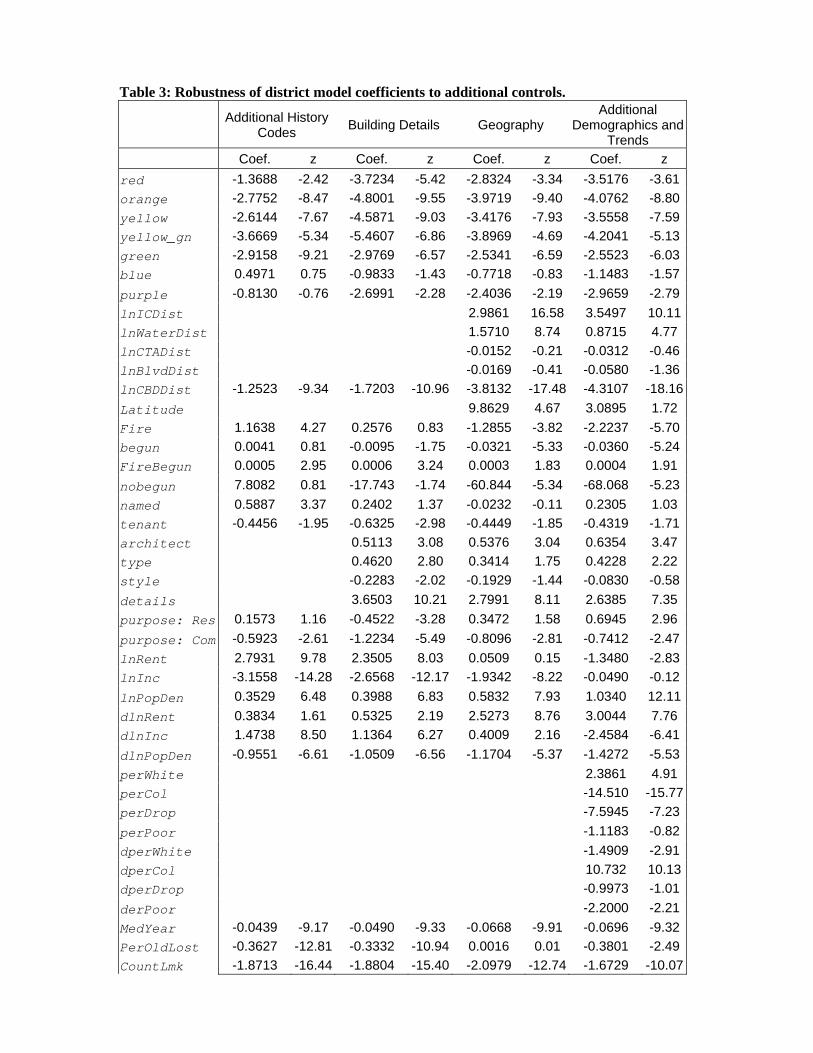
Table 3: Robustness of district model coefficients to additional controls.
Additional History Codes Building Details Geography
Additional Demographics and
Trends Coef. z Coef. z Coef. z Coef. z red -1.3688 -2.42 -3.7234 -5.42 -2.8324 -3.34 -3.5176 -3.61orange -2.7752 -8.47 -4.8001 -9.55 -3.9719 -9.40 -4.0762 -8.80yellow -2.6144 -7.67 -4.5871 -9.03 -3.4176 -7.93 -3.5558 -7.59yellow_gn -3.6669 -5.34 -5.4607 -6.86 -3.8969 -4.69 -4.2041 -5.13green -2.9158 -9.21 -2.9769 -6.57 -2.5341 -6.59 -2.5523 -6.03blue 0.4971 0.75 -0.9833 -1.43 -0.7718 -0.83 -1.1483 -1.57purple -0.8130 -0.76 -2.6991 -2.28 -2.4036 -2.19 -2.9659 -2.79lnICDist 2.9861 16.58 3.5497 10.11lnWaterDist 1.5710 8.74 0.8715 4.77 lnCTADist -0.0152 -0.21 -0.0312 -0.46lnBlvdDist -0.0169 -0.41 -0.0580 -1.36lnCBDDist -1.2523 -9.34 -1.7203 -10.96 -3.8132 -17.48 -4.3107 -18.16Latitude 9.8629 4.67 3.0895 1.72 Fire 1.1638 4.27 0.2576 0.83 -1.2855 -3.82 -2.2237 -5.70begun 0.0041 0.81 -0.0095 -1.75 -0.0321 -5.33 -0.0360 -5.24FireBegun 0.0005 2.95 0.0006 3.24 0.0003 1.83 0.0004 1.91 nobegun 7.8082 0.81 -17.743 -1.74 -60.844 -5.34 -68.068 -5.23named 0.5887 3.37 0.2402 1.37 -0.0232 -0.11 0.2305 1.03 tenant -0.4456 -1.95 -0.6325 -2.98 -0.4449 -1.85 -0.4319 -1.71architect 0.5113 3.08 0.5376 3.04 0.6354 3.47 type 0.4620 2.80 0.3414 1.75 0.4228 2.22 style -0.2283 -2.02 -0.1929 -1.44 -0.0830 -0.58details 3.6503 10.21 2.7991 8.11 2.6385 7.35 purpose: Res 0.1573 1.16 -0.4522 -3.28 0.3472 1.58 0.6945 2.96 purpose: Com -0.5923 -2.61 -1.2234 -5.49 -0.8096 -2.81 -0.7412 -2.47lnRent 2.7931 9.78 2.3505 8.03 0.0509 0.15 -1.3480 -2.83lnInc -3.1558 -14.28 -2.6568 -12.17 -1.9342 -8.22 -0.0490 -0.12lnPopDen 0.3529 6.48 0.3988 6.83 0.5832 7.93 1.0340 12.11dlnRent 0.3834 1.61 0.5325 2.19 2.5273 8.76 3.0044 7.76 dlnInc 1.4738 8.50 1.1364 6.27 0.4009 2.16 -2.4584 -6.41dlnPopDen -0.9551 -6.61 -1.0509 -6.56 -1.1704 -5.37 -1.4272 -5.53perWhite 2.3861 4.91 perCol -14.510 -15.77perDrop -7.5945 -7.23perPoor -1.1183 -0.82dperWhite -1.4909 -2.91dperCol 10.732 10.13dperDrop -0.9973 -1.01derPoor -2.2000 -2.21MedYear -0.0439 -9.17 -0.0490 -9.33 -0.0668 -9.91 -0.0696 -9.32PerOldLost -0.3627 -12.81 -0.3332 -10.94 0.0016 0.01 -0.3801 -2.49CountLmk -1.8713 -16.44 -1.8804 -15.40 -2.0979 -12.74 -1.6729 -10.07
CountCHRS 0.0566 31.42 0.0499 26.95 0.0407 18.95 0.0493 18.90Constant 80.480 5.86 110.882 7.11 -206.732 -2.19 77.962 0.97 Pseudo R-sq 0.5433 0.5814 0.6748 0.7109 Observations 13,832 13,832 13,602 13,602 Log likelihood -1,562.8301 -1,432.2516 -1,107.5842 -984.66176

Table 4: District designation models: robustness to different samples. CHRS MLS
Coef. z Coef. z Coef. z
CHRSprop 1.5850 6.71 1.3928 5.98
CHRS*orange -0.9231 -6.61 -1.5503 -5.24 -1.4431 -5.09
CHRS*green -1.4072 -7.92 -0.5753 -1.49 -0.3129 -0.70
lnWaterDist 1.1900 9.26 0.3417 1.87 0.5430 2.55
lnCTADist 0.4147 6.00 0.5938 9.19 0.4681 6.47
lnCBDDist -2.5312 -14.58 -0.6342 -2.89 -0.8673 -4.08
Latitude -0.1352 -0.09 -9.6841 -4.12 -11.836 -4.82
Fire 0.2019 0.76 -11.892 -1.80 -11.097 -1.44
begun -0.0148 -2.62 -0.0130 -5.48 -0.0114 -4.32
FireBegun 0.0003 2.07 0.0064 1.90 0.0058 1.46
nobegun -27.716 -2.59
named 0.5147 2.64 1.3052 4.95 1.6860 6.20
lnArea 2.4872 10.77
units -0.0043 -5.98
units-squared 0.0000 5.42
rooms -0.0870 -1.22
Bedrms -0.2273 -1.31
baths -0.9696 -6.15
firepl -0.0906 -0.70
parking -0.9710 -6.44
saleyr -0.0987 -3.34
lnRent 0.9845 2.59 2.2878 3.83 2.8451 4.33
lnInc -1.4933 -5.29 5.5425 9.76 5.0395 9.17
lnPopDen 1.2062 15.34 1.6919 11.36 1.7423 10.33
dlnRent 1.1052 3.44 1.1463 1.85 0.8000 1.21
dlnInc -0.7078 -2.66 -7.5869 -12.07 -7.2306 -11.75
dlnPopDen -1.3984 -8.89 3.5759 7.41 3.3327 7.31
perWhite 2.4662 7.01 6.3154 9.82 6.3310 9.74
perCol9 -13.306 -16.77 -17.758 -8.70 -17.468 -8.34
perPoor 3.5621 3.99 31.347 16.77 30.984 16.75
perDrop -12.946 -17.88 -11.417 -7.89 -10.980 -7.65
dperWhite 0.4967 1.25 1.7794 4.04 1.7312 3.42
dperCol9 10.631 11.86 19.499 7.51 18.912 7.15
dperPoor -4.4433 -5.85 -26.342 -15.56 -25.167 -15.00
dperDrop 3.5653 5.06 11.534 5.39 10.465 5.25
MedYear -0.0652 -9.64 -0.0913 -17.78 -0.0816 -12.53
PerOldLost -0.3281 -3.83 0.0002 0.00 -0.1111 -1.01
CountLmk -1.2922 -10.35 -0.3154 -2.95 -0.1166 -0.95
CountCHRS 0.0630 29.26 0.0735 20.84 0.0760 20.53
PerOldLost 156.75 2.28 514.15 5.09 765.13 6.34
PseudoR-sq 0.6028 0.6016 0.6299
Observations 13,832 61,915 59,381
Log Likelihood -1,359.1706 -1,340.5757 -1,217.4777